package pgfplots manual - ctan.math.washington.edu

Manual for Package PgfplotsTableComponent of pgfplots, Version 1.18.1

http://sourceforge.net/projects/pgfplots

Dr. Christian Feuersä[email protected]

Revision 1.18.1 (2021/05/15)

Abstract

This package reads tab-separated numerical tables from input and generates code for pretty-printedLATEX-tabulars. It rounds to the desired precision and prints it in different number formatting styles.

Contents1 Introduction 2

2 Loading and Displaying data 22.1 Text Table Input Format . . . . . . . . . . . . . . . . . . . . . . . . . . . . . . . . . . . . . . 22.2 Selecting Columns and their Appearance Styles . . . . . . . . . . . . . . . . . . . . . . . . . . 102.3 Configuring Row Appearance: Styles . . . . . . . . . . . . . . . . . . . . . . . . . . . . . . . . 172.4 Configuring Single Cell Appearance: Styles . . . . . . . . . . . . . . . . . . . . . . . . . . . . 222.5 Customizing and Getting the Tabular Code . . . . . . . . . . . . . . . . . . . . . . . . . . . . 232.6 Defining Column Types for tabular . . . . . . . . . . . . . . . . . . . . . . . . . . . . . . . . 262.7 Number Formatting Options . . . . . . . . . . . . . . . . . . . . . . . . . . . . . . . . . . . . 27

2.7.1 Changing Number Format Display Styles . . . . . . . . . . . . . . . . . . . . . . . . . 32

3 From Input Data To Output Tables: Data Processing 373.1 Loading the table . . . . . . . . . . . . . . . . . . . . . . . . . . . . . . . . . . . . . . . . . . . 373.2 Typesetting Cell Content . . . . . . . . . . . . . . . . . . . . . . . . . . . . . . . . . . . . . . 373.3 Preprocessing Cell Content . . . . . . . . . . . . . . . . . . . . . . . . . . . . . . . . . . . . . 403.4 Postprocessing Cell Content . . . . . . . . . . . . . . . . . . . . . . . . . . . . . . . . . . . . . 45

4 Generating Data in New Tables or Columns 474.1 Creating New Tables From Scratch . . . . . . . . . . . . . . . . . . . . . . . . . . . . . . . . . 474.2 Creating New Columns From Existing Ones . . . . . . . . . . . . . . . . . . . . . . . . . . . . 484.3 Predefined Column Generation Methods . . . . . . . . . . . . . . . . . . . . . . . . . . . . . . 51

4.3.1 Acquiring Data Somewhere . . . . . . . . . . . . . . . . . . . . . . . . . . . . . . . . . 514.3.2 Mathematical Operations . . . . . . . . . . . . . . . . . . . . . . . . . . . . . . . . . . 52

5 Miscellaneous 585.1 Writing (Modified) Tables To Disk . . . . . . . . . . . . . . . . . . . . . . . . . . . . . . . . . 585.2 Miscellaneous Keys . . . . . . . . . . . . . . . . . . . . . . . . . . . . . . . . . . . . . . . . . . 595.3 A summary of how to define and use styles and keys . . . . . . . . . . . . . . . . . . . . . . . 595.4 Plain TEX and ConTEXt support . . . . . . . . . . . . . . . . . . . . . . . . . . . . . . . . . . 605.5 Basic Level Table Access and Modification . . . . . . . . . . . . . . . . . . . . . . . . . . . . . 605.6 Repeating Things: Loops . . . . . . . . . . . . . . . . . . . . . . . . . . . . . . . . . . . . . . 66

Index 68

1

http://sourceforge.net/projects/pgfplots

1 IntroductionPgfplotsTable is a lightweight sub-package of pgfplots which employs its table input methods and thenumber formatting techniques to convert tab-separated tables into tabulars.

Its input is a text file containing space-separated rows, possibly starting with column names. Its outputis a LATEX tabular1 which contains selected columns of the text table, rounded to the desired precision,printed in the desired number format (fixed point, integer, scientific etc.). The output is LATEX code, andthat code is finally typeset by LATEX.

In other words, PgfplotsTable is nothing but a more-or-less smart code generator which spits outsomething like \begin{tabular}...\end{tabular}. Use it if you’d like to customize row or column depen-dent styles or if you have numerical data for which you want to have automatically formatted content.

It is used with

\usepackage{pgfplotstable}% recommended:%\usepackage{booktabs}%\usepackage{array}%\usepackage{colortbl}

and requires pgfplots and pgf ≥ 2.00 installed.

\pgfplotstableset{〈key-value-options〉}The user interface of this package is based on key-value-options. They determine what to display, howto format and what to compute.Key–value pairs can be set in two ways:

1. As default settings for the complete document (or maybe a part of the document), using\pgfplotstableset{〈options〉}. For example, the document’s preamble may contain

\pgfplotstableset{fixed zerofill,precision=3}

to configure a precision of 3 digits after the period, including zeros to get exactly 3 digits for allfixed point numbers.

2. As option which affects just a single table. This is provided as optional argument to the respectivetable typesetting command, for example \pgfplotstabletypeset[〈options〉]{〈file〉}.

Both ways are shown in the examples below.Knowledge of pgfkeys is useful for a deeper insight into this package, as /.style, /.append styleetc. are specific to pgfkeys. Please refer to the pgf manual [2, Section “pgfkeys”] or the shorterintroduction [3] to learn more about pgfkeys. Otherwise, simply skip over to the examples provided inthis document.You will find key prefixes /pgfplots/table/ and /pgf/number format/. These prefixes can be skippedif they are used in PgfplotsTable; they belong to the “default key path” of pgfkeys.

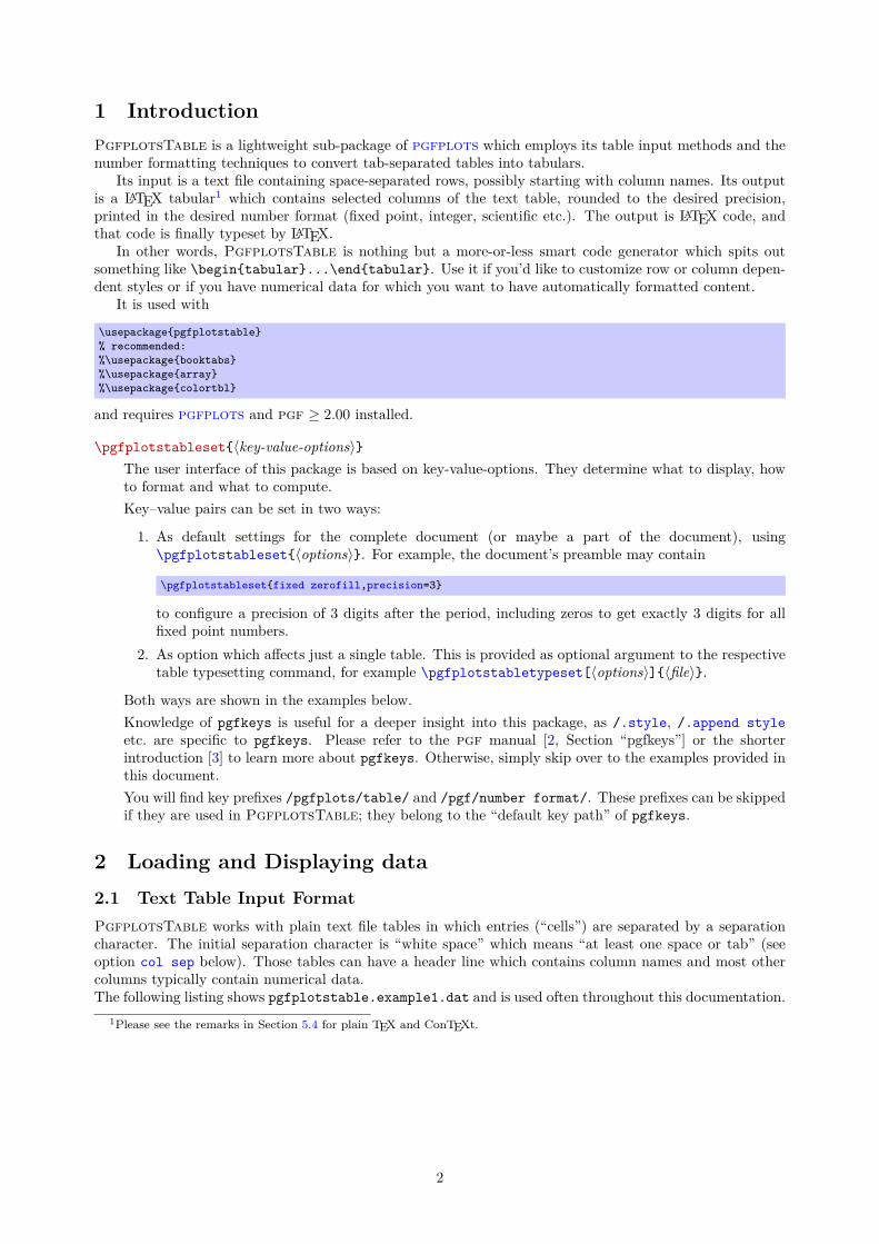
2 Loading and Displaying data2.1 Text Table Input FormatPgfplotsTable works with plain text file tables in which entries (“cells”) are separated by a separationcharacter. The initial separation character is “white space” which means “at least one space or tab” (seeoption col sep below). Those tables can have a header line which contains column names and most othercolumns typically contain numerical data.The following listing shows pgfplotstable.example1.dat and is used often throughout this documentation.

1Please see the remarks in Section 5.4 for plain TEX and ConTEXt.

2

# Convergence results# fictional source, generated 2008level dof error1 error2 info grad(log(dof),log(error2)) quot(error1)1 4 2.50000000e-01 7.57858283e-01 48 0 02 16 6.25000000e-02 5.00000000e-01 25 -3.00000000e-01 43 64 1.56250000e-02 2.87174589e-01 41 -3.99999999e-01 44 256 3.90625000e-03 1.43587294e-01 8 -5.00000003e-01 45 1024 9.76562500e-04 4.41941738e-02 22 -8.49999999e-01 46 4096 2.44140625e-04 1.69802322e-02 46 -6.90000001e-01 47 16384 6.10351562e-05 8.20091159e-03 40 -5.24999999e-01 48 65536 1.52587891e-05 3.90625000e-03 48 -5.35000000e-01 3.99999999e+009 262144 3.81469727e-06 1.95312500e-03 33 -5.00000000e-01 4.00000001e+0010 1048576 9.53674316e-07 9.76562500e-04 2 -5.00000000e-01 4.00000001e+00

Lines starting with ‘%’ or ‘#’ are considered to be comment lines and are ignored.

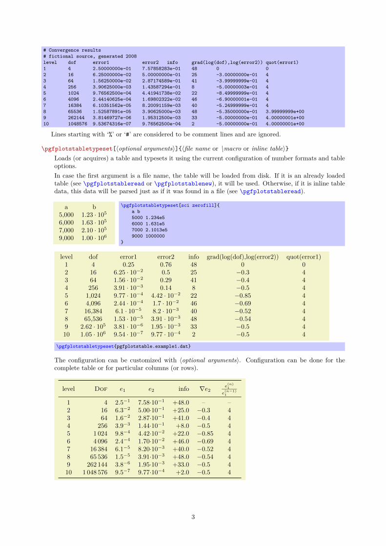
\pgfplotstabletypeset[〈optional arguments〉]{〈file name or \macro or inline table〉}Loads (or acquires) a table and typesets it using the current configuration of number formats and tableoptions.In case the first argument is a file name, the table will be loaded from disk. If it is an already loadedtable (see \pgfplotstableread or \pgfplotstablenew), it will be used. Otherwise, if it is inline tabledata, this data will be parsed just as if it was found in a file (see \pgfplotstableread).

a b5,000 1.23 · 1056,000 1.63 · 1057,000 2.10 · 1059,000 1.00 · 106

\pgfplotstabletypeset[sci zerofill]{a b5000 1.234e56000 1.631e57000 2.1013e59000 1000000

}

level dof error1 error2 info grad(log(dof),log(error2)) quot(error1)1 4 0.25 0.76 48 0 02 16 6.25 · 10−2 0.5 25 −0.3 43 64 1.56 · 10−2 0.29 41 −0.4 44 256 3.91 · 10−3 0.14 8 −0.5 45 1,024 9.77 · 10−4 4.42 · 10−2 22 −0.85 46 4,096 2.44 · 10−4 1.7 · 10−2 46 −0.69 47 16,384 6.1 · 10−5 8.2 · 10−3 40 −0.52 48 65,536 1.53 · 10−5 3.91 · 10−3 48 −0.54 49 2.62 · 105 3.81 · 10−6 1.95 · 10−3 33 −0.5 410 1.05 · 106 9.54 · 10−7 9.77 · 10−4 2 −0.5 4

\pgfplotstabletypeset{pgfplotstable.example1.dat}

The configuration can be customized with 〈optional arguments〉. Configuration can be done for thecomplete table or for particular columns (or rows).

level Dof e1 e2 info ∇e2e(n)1

e(n−1)1

1 4 2.5−1 7.58·10−1 +48.0 – –2 16 6.3−2 5.00·10−1 +25.0 −0.3 43 64 1.6−2 2.87·10−1 +41.0 −0.4 44 256 3.9−3 1.44·10−1 +8.0 −0.5 45 1 024 9.8−4 4.42·10−2 +22.0 −0.85 46 4 096 2.4−4 1.70·10−2 +46.0 −0.69 47 16 384 6.1−5 8.20·10−3 +40.0 −0.52 48 65 536 1.5−5 3.91·10−3 +48.0 −0.54 49 262 144 3.8−6 1.95·10−3 +33.0 −0.5 410 1 048 576 9.5−7 9.77·10−4 +2.0 −0.5 4

3

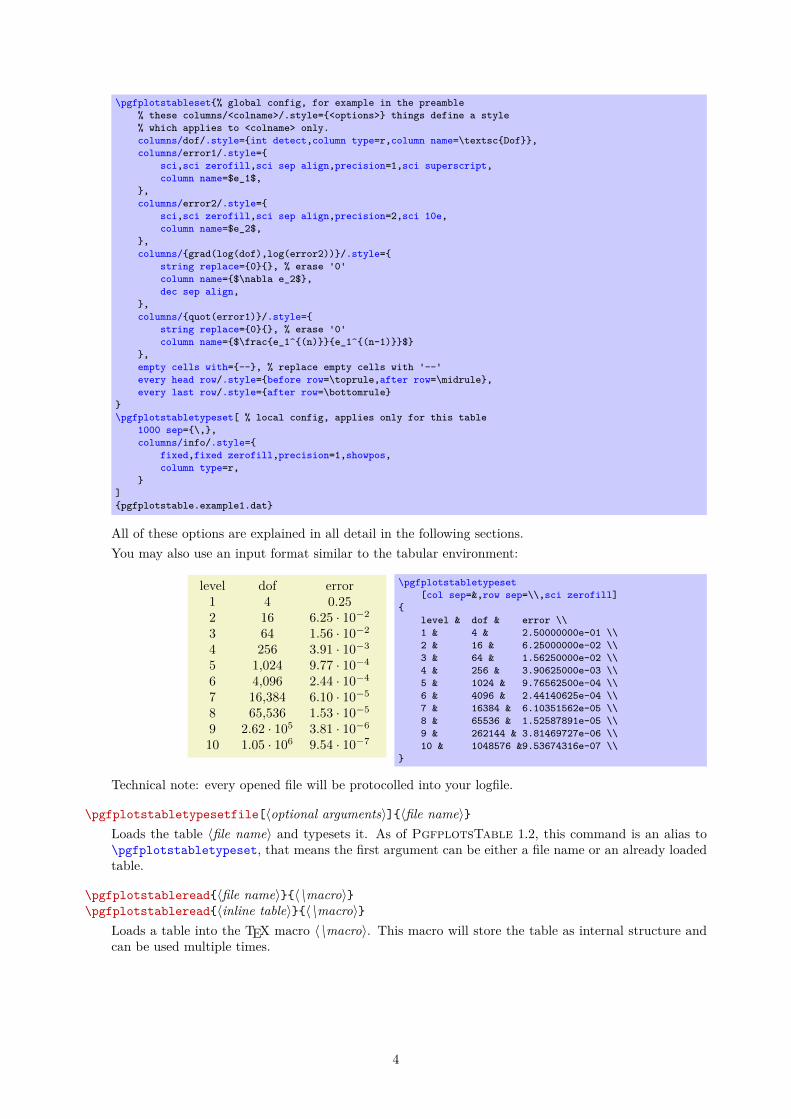
\pgfplotstableset{% global config, for example in the preamble% these columns/<colname>/.style={<options>} things define a style% which applies to <colname> only.columns/dof/.style={int detect,column type=r,column name=\textsc{Dof}},columns/error1/.style={

sci,sci zerofill,sci sep align,precision=1,sci superscript,column name=$e_1$,

},columns/error2/.style={

sci,sci zerofill,sci sep align,precision=2,sci 10e,column name=$e_2$,

},columns/{grad(log(dof),log(error2))}/.style={

string replace={0}{}, % erase '0'column name={$\nabla e_2$},dec sep align,

},columns/{quot(error1)}/.style={

string replace={0}{}, % erase '0'column name={$\frac{e_1^{(n)}}{e_1^{(n-1)}}$}

},empty cells with={--}, % replace empty cells with '--'every head row/.style={before row=\toprule,after row=\midrule},every last row/.style={after row=\bottomrule}

}\pgfplotstabletypeset[ % local config, applies only for this table

1000 sep={\,},columns/info/.style={

fixed,fixed zerofill,precision=1,showpos,column type=r,

}]{pgfplotstable.example1.dat}

All of these options are explained in all detail in the following sections.You may also use an input format similar to the tabular environment:

level dof error1 4 0.252 16 6.25 · 10−2

3 64 1.56 · 10−2

4 256 3.91 · 10−3

5 1,024 9.77 · 10−4

6 4,096 2.44 · 10−4

7 16,384 6.10 · 10−5

8 65,536 1.53 · 10−5

9 2.62 · 105 3.81 · 10−6

10 1.05 · 106 9.54 · 10−7

\pgfplotstabletypeset[col sep=&,row sep=\\,sci zerofill]

{level & dof & error \\1 & 4 & 2.50000000e-01 \\2 & 16 & 6.25000000e-02 \\3 & 64 & 1.56250000e-02 \\4 & 256 & 3.90625000e-03 \\5 & 1024 & 9.76562500e-04 \\6 & 4096 & 2.44140625e-04 \\7 & 16384 & 6.10351562e-05 \\8 & 65536 & 1.52587891e-05 \\9 & 262144 & 3.81469727e-06 \\10 & 1048576 &9.53674316e-07 \\

}

Technical note: every opened file will be protocolled into your logfile.

\pgfplotstabletypesetfile[〈optional arguments〉]{〈file name〉}Loads the table 〈file name〉 and typesets it. As of PgfplotsTable 1.2, this command is an alias to\pgfplotstabletypeset, that means the first argument can be either a file name or an already loadedtable.

\pgfplotstableread{〈file name〉}{〈\macro〉}\pgfplotstableread{〈inline table〉}{〈\macro〉}

Loads a table into the TEX macro 〈\macro〉. This macro will store the table as internal structure andcan be used multiple times.

4

dof error14 0.2516 6.25 · 10−2

64 1.56 · 10−2

256 3.91 · 10−3

1,024 9.77 · 10−4

4,096 2.44 · 10−4

16,384 6.1 · 10−5

65,536 1.53 · 10−5

2.62 · 105 3.81 · 10−6

1.05 · 106 9.54 · 10−7

dof error24 0.7616 0.564 0.29256 0.141,024 4.42 · 10−2

4,096 1.7 · 10−2

16,384 8.2 · 10−3

65,536 3.91 · 10−3

2.62 · 105 1.95 · 10−3

1.05 · 106 9.77 · 10−4

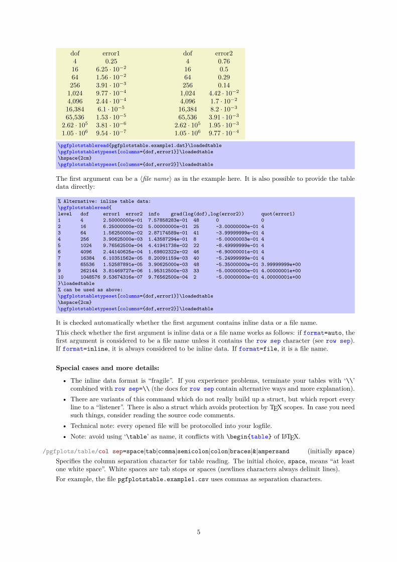
\pgfplotstableread{pgfplotstable.example1.dat}\loadedtable\pgfplotstabletypeset[columns={dof,error1}]\loadedtable\hspace{2cm}\pgfplotstabletypeset[columns={dof,error2}]\loadedtable

The first argument can be a 〈file name〉 as in the example here. It is also possible to provide the tabledata directly:

% Alternative: inline table data:\pgfplotstableread{level dof error1 error2 info grad(log(dof),log(error2)) quot(error1)1 4 2.50000000e-01 7.57858283e-01 48 0 02 16 6.25000000e-02 5.00000000e-01 25 -3.00000000e-01 43 64 1.56250000e-02 2.87174589e-01 41 -3.99999999e-01 44 256 3.90625000e-03 1.43587294e-01 8 -5.00000003e-01 45 1024 9.76562500e-04 4.41941738e-02 22 -8.49999999e-01 46 4096 2.44140625e-04 1.69802322e-02 46 -6.90000001e-01 47 16384 6.10351562e-05 8.20091159e-03 40 -5.24999999e-01 48 65536 1.52587891e-05 3.90625000e-03 48 -5.35000000e-01 3.99999999e+009 262144 3.81469727e-06 1.95312500e-03 33 -5.00000000e-01 4.00000001e+0010 1048576 9.53674316e-07 9.76562500e-04 2 -5.00000000e-01 4.00000001e+00}\loadedtable% can be used as above:\pgfplotstabletypeset[columns={dof,error1}]\loadedtable\hspace{2cm}\pgfplotstabletypeset[columns={dof,error2}]\loadedtable

It is checked automatically whether the first argument contains inline data or a file name.This check whether the first argument is inline data or a file name works as follows: if format=auto, thefirst argument is considered to be a file name unless it contains the row sep character (see row sep).If format=inline, it is always considered to be inline data. If format=file, it is a file name.

Special cases and more details:

• The inline data format is “fragile”. If you experience problems, terminate your tables with ‘\\’combined with row sep=\\ (the docs for row sep contain alternative ways and more explanation).

• There are variants of this command which do not really build up a struct, but which report everyline to a “listener”. There is also a struct which avoids protection by TEX scopes. In case you needsuch things, consider reading the source code comments.

• Technical note: every opened file will be protocolled into your logfile.• Note: avoid using ‘\table’ as name, it conflicts with \begin{table} of LATEX.

/pgfplots/table/col sep=space|tab|comma|semicolon|colon|braces|&|ampersand (initially space)Specifies the column separation character for table reading. The initial choice, space, means “at leastone white space”. White spaces are tab stops or spaces (newlines characters always delimit lines).For example, the file pgfplotstable.example1.csv uses commas as separation characters.

5

# Convergence results# fictional source generated 2008level,dof,error1,error2,info,{grad(log(dof),log(error2))},quot(error1)1,9,2.50000000e-01,7.57858283e-01,48,0,02,25,6.25000000e-02,5.00000000e-01,25,-1.35691545e+00,43,81,1.56250000e-02,2.87174589e-01,41,-1.17924958e+00,44,289,3.90625000e-03,1.43587294e-01,8,-1.08987331e+00,45,1089,9.76562500e-04,4.41941738e-02,22,-1.04500712e+00,46,4225,2.44140625e-04,1.69802322e-02,46,-1.02252239e+00,47,16641,6.10351562e-05,8.20091159e-03,40,-1.01126607e+00,48,66049,1.52587891e-05,3.90625000e-03,48,-1.00563427e+00,3.99999999e+009,263169,3.81469727e-06,1.95312500e-03,33,-1.00281745e+00,4.00000001e+0010,1050625,9.53674316e-07,9.76562500e-04,2,-1.00140880e+00,4.00000001e+00

Thus, we need to specify col sep=comma when we read it.


\pgfplotstabletypeset[col sep=comma]{pgfplotstable.example1.csv}

You may call \pgfplotstableset{col sep=comma} once in your preamble if all your tables use commasas column separator.Please note that if cell entries (for example column names) contain the separation character, you needto enclose the column entry in braces: {grad(log(dof),log(error2)}. If you want to use unmatchedbraces, you need to write a backslash before the brace. For example the name ‘column{withbrace’needs to be written as ‘column\{withbrace’.For col sep6=space, spaces will be considered to be part of the argument (there is no trimming).However, (as usual in TEX), multiple successive spaces and tabs are replace by a single white space. Ofcourse, if col sep=tab, tabs are the column separators and will be treated specially.Furthermore, if you need empty cells in case col sep=space, you have to provide {} to delimit such acell since col sep=space uses at least one white space (consuming all following ones).The value col sep=braces is special since it actually uses two separation characters. Every single cellentry is delimited by an opening and a closing brace, 〈entry〉, for this choice. Furthermore, any whitespace (spaces and tabs) between cell entries are skipped in case braces until the next 〈entry〉 is found.A further specialty of col sep=braces is that it has support for multi-line cells: everything withinbalanced braces is considered to be part of a cell. This includes newlines:2

The col sep=& case (probably together with row sep=\\) allows to read tables as you’d usually typethem in LATEX. This will automatically enable trim cells.

/pgfplots/table/trim cells=true|false (initially false)If enabled, leading and trailing white space will be removed while tables are read.This might be necessary if you have col sep6=space but your cells contain spaces. It will be activatedautomatically for col sep=&.

/pgfplots/table/header=true|false|has colnames (initially true)Configures if column names shall be identified automatically during input operations.

2This treatment of newlines within balanced braces actually applies to every other column separator as well (it is a TEXreadline feature). In other words: you can have multi-line cells for every column separator if you enclose them in balanced curlybraces. However, col sep=braces has the special treatment that end-of-line counts as white space character; for every othercol sep value, this white space is suppressed to remove spurious spaces.

6

The first non-comment line can be a header which contains column names. The header key configureshow to detect if that is really the case.The choice true enables auto detection of column names: If the first non-comment line contains atleast one non-numerical entry (for example ‘a name’), each entry in this line is supposed to be a columnname. If the first non-comment line contains only numerical data, it is used as data row. In this case,column indices will be assigned as column “names”.The choice false is identical to this last case, i.e. even if the first line contains strings, they won’t berecognised as column names.Finally, the choice has colnames is the opposite of false: it assumes that the first non-comment linecontains column names. In other words: even if only numbers are contained in the first line, they areconsidered to be column names.Note that this key only configures headers in input tables. To configure output headers, you may wantto look at every head row.

/pgfplots/table/format=auto|inline|file (initially auto)Configures the format expected as first argument for \pgfplotstableread{〈input〉}.The choice inline expects the table data directly as argument where rows are separated by row sep.Inline data is “fragile”, because TEX may consume end-of-line characters (or col sep characters). Seerow sep for details.The choice file expects a file name.The choice auto searches for a row sep in the first argument supplied to \pgfplotstableread. If arow sep has been found, it is inline data, otherwise it is a file name.

/pgfplots/table/row sep=newline|\\ (initially newline)Configures the character to separate rows of the inline table data format (see format=inline).The choice newline uses the end of line as it appears in the table data (i.e. the input file or any inlinetable data).The choice \\ uses ‘\\’ to indicate the end of a row.Note that newline for inline table data is “fragile”: you can’t provide such data inside of TEX macros(this does not apply to input files). Whenever you experience problems, proceed as follows:

1. First possibility: call \pgfplotstableread{〈data〉}\yourmacro outside of any macro declaration.2. Use row sep=\\.

The same applies if you experience problems with inline data and special col sep choices (like colsep=tab).The reasons for such problems is that TEX scans the macro bodies and replaces newlines by white space.It does other substitutions of this sort as well, and these substitutions can’t be undone (maybe not evenfound).

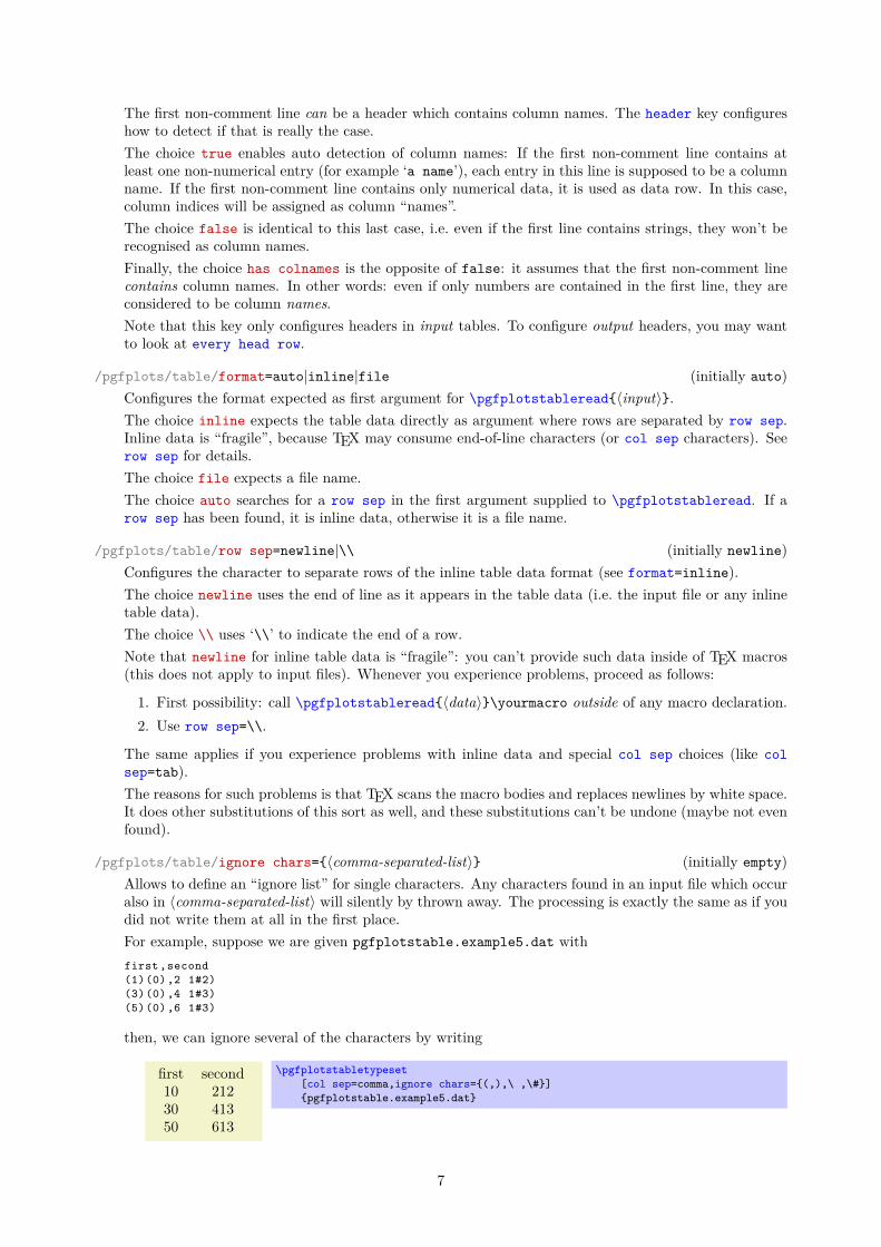
/pgfplots/table/ignore chars={〈comma-separated-list〉} (initially empty)Allows to define an “ignore list” for single characters. Any characters found in an input file which occuralso in 〈comma-separated-list〉 will silently by thrown away. The processing is exactly the same as if youdid not write them at all in the first place.For example, suppose we are given pgfplotstable.example5.dat withfirst,second(1)(0),2 1#2)(3)(0),4 1#3)(5)(0),6 1#3)

then, we can ignore several of the characters by writing

first second10 21230 41350 613

\pgfplotstabletypeset[col sep=comma,ignore chars={(,),\ ,\#}]{pgfplotstable.example5.dat}

7

The 〈comma-separated-list〉 should contain exactly one character in each list element, and the singlecharacters should be separated by commas. Some special characters like commas, white space, hashes,percents or backslashes need to be escaped by prefixing them with a backslash.Besides normal characters, it is also supported to eliminate any binary code from your input files. Forexample, suppose you have binary characters of code 0x01 (hex notation) in your files. Then, use

\pgfplotstableset{ignore chars={\^^01}}

to eliminate them silently. The ^^〈digit〉〈digit〉 notation is a TEX feature to provide characters inhexadecimal encoding where 〈digit〉 is one of 0123456789abcdef. I don’t know if the backslash in\^^01 is always necessary, try it out. There is also a character based syntax, in which \^^M is 〈newline〉and \^^I is 〈tab〉. Refer to [1] for more details.Note that after stripping all these characters, the input table must be valid – it should still containcolumn separators and balanced columns.This setting applies to \addplot table and \addplot file for pgfplots as well.Note that ignore chars is “fragile” when it is applied to format=inline or format=auto. Considerformat=file if you experience problems.3

/pgfplots/table/white space chars={〈comma-separated-list〉} (initially empty)Allows to define a list of single characters which are actually treated like white space (in addition totabs and spaces). It might be useful in order to get more than one column separator character.The white space chars list is used in exactly the same way as ignore chars, and the same remarksas above apply as well.

/pgfplots/table/text special chars={〈comma-separated-list〉} (initially empty)Allows to define a list of single characters which are actually treated like normal text (like any characterswith category code 12).The text special chars list is used in exactly the same way as ignore chars, and the same remarksas above apply as well.Note that some (selected) special characters are installed by verb string type.

URIhttp://example.org/a#b

\pgfplotstabletypeset[font=\ttfamily,verb string type,

]{URIhttp://example.org/a#b}

/pgfplots/table/comment chars={〈comma-separated-list〉} (initially empty)Allows to add one or more additional comment characters. Each of these characters has a similar effectas the # character, i.e. all following characters of that particular input line are skipped.

0 11 02 −103 0

\pgfplotstabletypeset[comment chars=!]{! Some comments1 02 -10! another comment line3 0}

The example above uses ‘!’ as additional comment character (which allows to parse Touchstone files).

/pgfplots/table/percent is letter=true|false (initially false)Allows to control how to treat percent characters in input files. PgfplotsTable used to keep the TEXspecial meaning as comment character which means that all characters following percent where ignored.

3See also row sep for more information about dealing with fragile inline table formats.

8

The value true means that a percent is just a normal letter without special meaning. The value falsemeans that percent is special as it used to be.

/pgfplots/table/text indicator={〈char〉} (initially empty)Allows to define a text indicator character. If this is defined, it can be used to enclose delimiters in acell’s body:

A BA long cell normalcell

\pgfplotstabletypeset[text indicator=",string type]{A B"A long cell" normalcell}

If the text indicator also occurs within the cell, it has to be doubled:

A BA long ”cell” normalcell

\pgfplotstabletypeset[text indicator=",string type]{A B"A long ""cell""" normalcell}

Cells which do not start with the text indicator are handled normally. Note that text indicator doesnot support multi-line cells.

/pgfplots/table/skip first n={〈integer〉} (initially 0)Allows to skip the first 〈integer〉 lines of an input file. The lines will not be processed.

A B C1 2 34 5 6

\pgfplotstabletypeset[skip first n=4]{%<- this '%' is important. Otherwise, the%newline here would delimit an (empty) row.

XYZ Format,Version 1.234Date 2010-09-01@author MustermannA B C1 2 34 5 6

}

/pgfplots/table/search path={〈comma-separated-list〉} (initially .)Allows to provide a search path for input tables. This variable is evaluated whenever pgfplots attemptsto read a data file. This includes both \pgfplotstableread and \addplot table; its value resemblesa comma-separated list of path names. The requested file will be read from the first matching locationin that list.Use ‘.’ to search using the normal TEX file searching procedure (i.e. typically in the current workingdirectory).An entry in 〈comma-separated-list〉 can be relative to the current working directory, i.e. something likesearch path={.,../datafiles} is accepted.

/pgfplots/table/search path/implicit .=true|false (initially true)PgfplotsTable allows to add ‘.’ to the value of search path implicitly as this is typically assumedin many applications of search paths.The initial configuration search path/implicit .=true will ensure that ‘.’ is added in front of thesearch path if the user value does not contain a ‘.’.The value search path/implicit .=false will not add ‘.’.Keep in mind that ‘.’ means “let TEX search for the file on its own”. This will typically find files in thecurrent working directory, but it will also include processing of TEXINPUTS.

9

2.2 Selecting Columns and their Appearance Styles/pgfplots/table/columns={〈comma-separated-list〉}

Selects particular columns of the table. If this option is empty (has not been provided), all availablecolumns will be selected.Inside of 〈comma-separated-list〉, column names as they appear in the table’s header are expected.If there is no header, simply use column indices. If there are column names, the special syntax[index]〈integer〉 can be used to select columns by index. The first column has index 0.

dof level info4 1 4816 2 2564 3 41256 4 81,024 5 224,096 6 4616,384 7 4065,536 8 48

2.62 · 105 9 331.05 · 106 10 2

\pgfplotstabletypeset[columns={dof,level,[index]4}]{pgfplotstable.example1.dat}

The special pgfkeys feature \pgfplotstableset{columns/.add={}{,a further col}} allows to ap-pend a value, in this case ‘,a further col’ to the actual value. See /.add for details.

/pgfplots/table/alias/〈col name〉/.initial={〈real col name〉}Assigns the new name 〈col name〉 for the column denoted by 〈real col name〉. Afterwards, accessing 〈colname〉 will use the data associated with column 〈real col name〉.

a newname1 23 45 6

% in preamble:\pgfplotstableset{

alias/newname/.initial=b,}

% in document:\pgfplotstabletypeset[

columns={a,newname},% access to `newname' is the same as to `b']{

a b1 23 45 6

}%

You can use columns/〈col name〉/.style to assign styles for the alias, not for the original column name.If there exists both an alias and a column of the same name, the column name will be preferred.Furthermore, if there exists a create on use statement with the same name, this one will also bepreferred.In case 〈col name〉 contains characters which are required for key settings, you need to use braces aroundit: “alias/{name=wi/th,special}/.initial={othername}”.This key is used whenever columns are queried, it applies also to the \addplot table statement ofpgfplots.

/pgfplots/table/columns/〈column name〉/.style={〈key-value-list〉}Sets all options in 〈key-value-list〉 exclusively for 〈column name〉.

10

level Dof L2 A info grad(log(dof),log(error2)) quot(error1)1 4 2.500−1 7.58−1 48 0 02 16 6.250−2 5.00−1 25 −0.3 43 64 1.563−2 2.87−1 41 −0.4 44 256 3.906−3 1.44−1 8 −0.5 45 1,024 9.766−4 4.42−2 22 −0.85 46 4,096 2.441−4 1.70−2 46 −0.69 47 16,384 6.104−5 8.20−3 40 −0.52 48 65,536 1.526−5 3.91−3 48 −0.54 49 262,144 3.815−6 1.95−3 33 −0.5 410 1,048,576 9.537−7 9.77−4 2 −0.5 4

\pgfplotstabletypeset[columns/error1/.style={

column name=$L_2$,sci,sci zerofill,sci subscript,precision=3},

columns/error2/.style={column name=$A$,sci,sci zerofill,sci subscript,precision=2},

columns/dof/.style={int detect,column name=\textsc{Dof}

}]

{pgfplotstable.example1.dat}

If your column name contains commas ‘,’, slashes ‘/’ or equal signs ‘=’, you need to enclose the columnname in braces.

Dof L2 slopes L2

4 2.500−1 0.016 6.250−2 −0.364 1.563−2 −0.4256 3.906−3 −0.51,024 9.766−4 −0.84,096 2.441−4 −0.716,384 6.104−5 −0.565,536 1.526−5 −0.5262,144 3.815−6 −0.51,048,576 9.537−7 −0.5

\pgfplotstabletypeset[columns={dof,error1,{grad(log(dof),log(error2))}},columns/error1/.style={


columns/dof/.style={int detect,column name=\textsc{Dof}},

columns/{grad(log(dof),log(error2))}/.style={column name=slopes $L_2$,fixed,fixed zerofill,precision=1}

]{pgfplotstable.example1.dat}

If your tables don’t have column names, you can simply use integer indices instead of 〈column name〉to refer to columns. If you have column names, you can’t set column styles using indices.

/pgfplots/table/display columns/〈index〉/.style={〈key-value-list〉}Applies all options in 〈key-value-list〉 exclusively to the column which will appear at position 〈index〉 inthe output table.In contrast to the table/columns/〈name〉 styles, this option refers to the output table instead of theinput table. Since the output table has no unique column name, you can only access columns by index.Indexing starts with 〈index〉 = 0.Display column styles override input column styles.

/pgfplots/table/every col no 〈index〉 (style, no value)A style which is identical with display columns/〈index〉: it applies exclusively to the column at position〈index〉 in the output table.See display columns/〈index〉 for details.

/pgfplots/table/column type={〈tabular column type〉} (initially c)

11

Contains the column type for tabular.If all column types are empty, the complete argument is skipped (assuming that no tabular environmentis generated).Use \pgfplotstableset{column type/.add={〈before〉}{〈after〉}} to modify a value instead of over-writing it. The /.add key handler works for other options as well.

dof error1 info4 0.25 4816 6.25 · 10−2 2564 1.56 · 10−2 41256 3.91 · 10−3 81,024 9.77 · 10−4 224,096 2.44 · 10−4 4616,384 6.1 · 10−5 4065,536 1.53 · 10−5 48

2.62 · 105 3.81 · 10−6 331.05 · 106 9.54 · 10−7 2

\pgfplotstabletypeset[columns={dof,error1,info},column type/.add={|}{}% results in '|c'


/pgfplots/table/column name={〈TEX display column name〉} (initially \pgfkeysnovalue)Sets the column’s display name in the current context.It is advisable to provide this option inside of a column-specific style, i.e. usingcolumns/{〈lowlevel colname〉}/.style={column name={〈TEX display column name〉}} .Here, “lowlevel colname” refers to the column name that is present in your input table. This lowlevelcolumn name has a couple of restrictions (it has to be expandable, for example – that means many controlsequences are forbidden). The value of column name is only used within \pgfplotstabletypeset inorder to generate a display name for the column in question.Note that you are allowed to provide an empty display name using column name={}. This results in anempty string above the column when used in \pgfplotstabletypeset.The initial configuration is column name=\pgfkeysnovalue. This constitutes a special “null” valuewhich tells \pgfplotstabletypeset that it should fall back to the column’s name (i.e. the lowlevelname).

/pgfplots/table/assign column name/.code={〈...〉}Allows to modify the value of column name.Argument #1 is the current column name, that means after evaluation of column name. After assigncolumn name, a new (possibly modified) value for column name should be set.That means you can use column name to assign the name as such and assign column name to generatefinal TEX code (for example to insert \multicolumn{1}{c}{#1}).

first second1 23 4

\pgfplotstabletypeset[assign column name/.style={

/pgfplots/table/column name={\textbf{#1}}},

]{first second1 23 4}

Note that the PgfplotsTable provides limited postprocessing capabilities for headers, in particular,postproc cell content and its friends merely apply to “normal” cells. If you want to modify theappearance of header cells, you should consider using assign column name.Default is empty which means no change.

/pgfplots/table/multicolumn names={〈tabular column type〉} (style, initially c)A style which typesets each column name in the current context using a \multicolumn{1}{〈tabularcolumn type〉}{〈the column name〉} statement.

12

Here,〈the column name〉 is set with column name as usual.

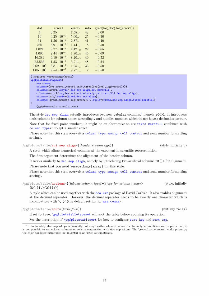
/pgfplots/table/dec sep align={〈header column type〉} (style, initially c)A style which aligns numerical columns at the decimal separator.The first argument determines the alignment of the header column.Please note that you need \usepackage{array} for this style.

dof error1 error2 info grad(log(dof),log(error2))4 0.25 7.58−1 48 016 6.25 · 10−2 5.00−1 25 −0.364 1.56 · 10−2 2.87−1 41 −0.4256 3.91 · 10−3 1.44−1 8 −0.51,024 9.77 · 10−4 4.42−2 22 −0.854,096 2.44 · 10−4 1.70−2 46 −0.6916,384 6.1 · 10−5 8.20−3 40 −0.5265,536 1.53 · 10−5 3.91−3 48 −0.54

2.62 · 105 3.81 · 10−6 1.95−3 33 −0.51.05 · 106 9.54 · 10−7 9.77−4 2 −0.5

% requires \usepackage{array}\pgfplotstabletypeset[

columns={dof,error1,error2,info,{grad(log(dof),log(error2))}},columns/error1/.style={dec sep align},columns/error2/.style={sci,sci subscript,sci zerofill,dec sep align},columns/info/.style={fixed,dec sep align},columns/{grad(log(dof),log(error2))}/.style={fixed,dec sep align}


Or with comma as decimal separator:

dof error1 error2 info grad(log(dof),log(error2))4 0,25 7,58−1 48 016 6,25 · 10−2 5,00−1 25 −0,364 1,56 · 10−2 2,87−1 41 −0,4256 3,91 · 10−3 1,44−1 8 −0,51.024 9,77 · 10−4 4,42−2 22 −0,854.096 2,44 · 10−4 1,70−2 46 −0,6916.384 6,1 · 10−5 8,20−3 40 −0,5265.536 1,53 · 10−5 3,91−3 48 −0,54

2,62 · 105 3,81 · 10−6 1,95−3 33 −0,51,05 · 106 9,54 · 10−7 9,77−4 2 −0,5


use comma,columns={dof,error1,error2,info,{grad(log(dof),log(error2))}},columns/error1/.style={dec sep align},columns/error2/.style={sci,sci subscript,sci zerofill,dec sep align},columns/info/.style={fixed,dec sep align},columns/{grad(log(dof),log(error2))}/.style={fixed,dec sep align}


It may be advisable to use fixed zerofill and/or sci zerofill to force at least one digit after thedecimal separator to improve placement of exponents:

13

dof error1 error2 info grad(log(dof),log(error2))4 0,25 7,58−1 48 0,0016 6,25 · 10−2 5,00−1 25 −0,3064 1,56 · 10−2 2,87−1 41 −0,40256 3,91 · 10−3 1,44−1 8 −0,501.024 9,77 · 10−4 4,42−2 22 −0,854.096 2,44 · 10−4 1,70−2 46 −0,6916.384 6,10 · 10−5 8,20−3 40 −0,5265.536 1,53 · 10−5 3,91−3 48 −0,54

2,62 · 105 3,81 · 10−6 1,95−3 33 −0,501,05 · 106 9,54 · 10−7 9,77−4 2 −0,50


use comma,columns={dof,error1,error2,info,{grad(log(dof),log(error2))}},columns/error1/.style={dec sep align,sci zerofill},columns/error2/.style={sci,sci subscript,sci zerofill,dec sep align},columns/info/.style={fixed,dec sep align},columns/{grad(log(dof),log(error2))}/.style={fixed,dec sep align,fixed zerofill}


The style dec sep align actually introduces two new tabular columns,4 namely r@{}l. It introducesmulticolumns for column names accordingly and handles numbers which do not have a decimal separator.Note that for fixed point numbers, it might be an alternative to use fixed zerofill combined withcolumn type=r to get a similar effect.Please note that this style overwrites column type, assign cell content and some number formattingsettings.

/pgfplots/table/sci sep align={〈header column type〉} (style, initially c)A style which aligns numerical columns at the exponent in scientific representation.The first argument determines the alignment of the header column.It works similarly to dec sep align, namely by introducing two artificial columns r@{}l for alignment.Please note that you need \usepackage{array} for this style.Please note that this style overwrites column type, assign cell content and some number formattingsettings.

/pgfplots/table/dcolumn={〈tabular column type〉}{〈type for column name〉} (style, initially{D{.}{.}{2}}{c})A style which can be used together with the dcolumn package of David Carlisle. It also enables alignmentat the decimal separator. However, the decimal separator needs to be exactly one character which isincompatible with ‘{,}’ (the default setting for use comma).

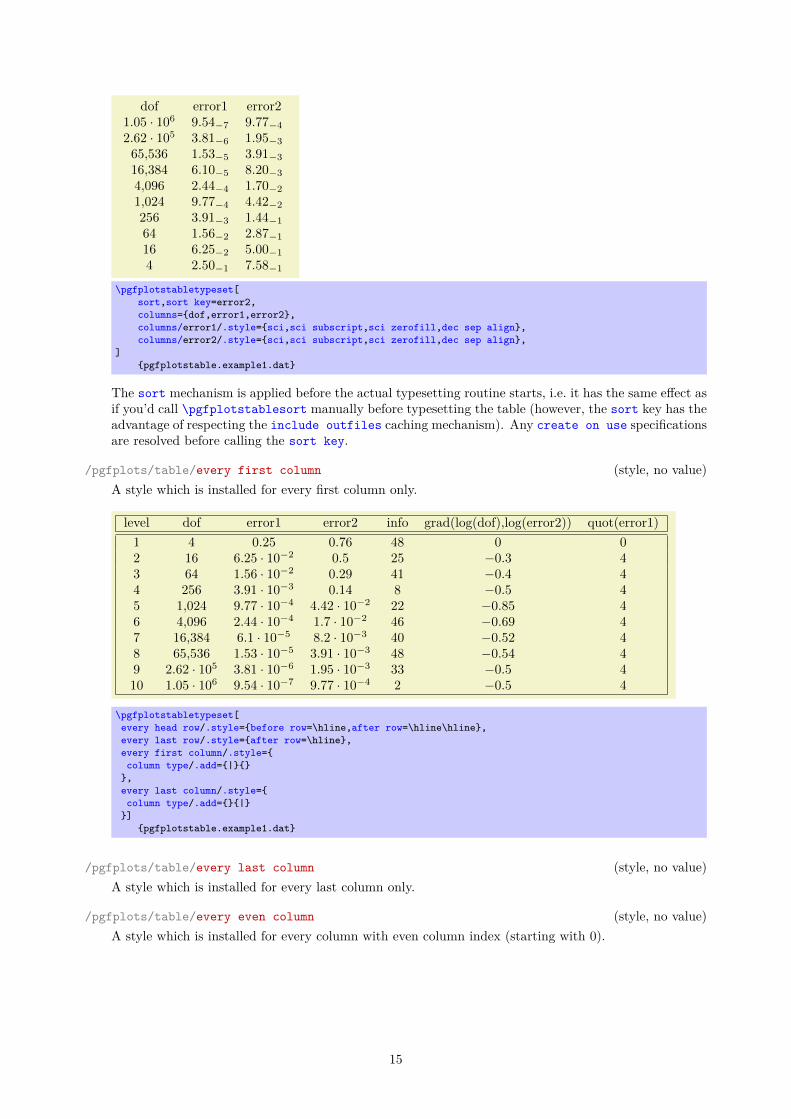
/pgfplots/table/sort={〈true,false〉} (initially false)If set to true, \pgfplotstabletypeset will sort the table before applying its operation.See the description of \pgfplotstablesort for how to configure sort key and sort cmp.

4Unfortunately, dec sep align is currently not very flexible when it comes to column type modifications. In particular, itis not possible to use colored columns or cells in conjunction with dec sep align. The \rowcolor command works properly;the color hangover introduced by colortbl is adjusted automatically.

14

dof error1 error21.05 · 106 9.54−7 9.77−4

2.62 · 105 3.81−6 1.95−3

65,536 1.53−5 3.91−3

16,384 6.10−5 8.20−3

4,096 2.44−4 1.70−2

1,024 9.77−4 4.42−2

256 3.91−3 1.44−1

64 1.56−2 2.87−1

16 6.25−2 5.00−1

4 2.50−1 7.58−1

\pgfplotstabletypeset[sort,sort key=error2,columns={dof,error1,error2},columns/error1/.style={sci,sci subscript,sci zerofill,dec sep align},columns/error2/.style={sci,sci subscript,sci zerofill,dec sep align},


The sort mechanism is applied before the actual typesetting routine starts, i.e. it has the same effect asif you’d call \pgfplotstablesort manually before typesetting the table (however, the sort key has theadvantage of respecting the include outfiles caching mechanism). Any create on use specificationsare resolved before calling the sort key.

/pgfplots/table/every first column (style, no value)A style which is installed for every first column only.


\pgfplotstabletypeset[every head row/.style={before row=\hline,after row=\hline\hline},every last row/.style={after row=\hline},every first column/.style={column type/.add={|}{}},every last column/.style={column type/.add={}{|}}]


/pgfplots/table/every last column (style, no value)A style which is installed for every last column only.

/pgfplots/table/every even column (style, no value)A style which is installed for every column with even column index (starting with 0).

15

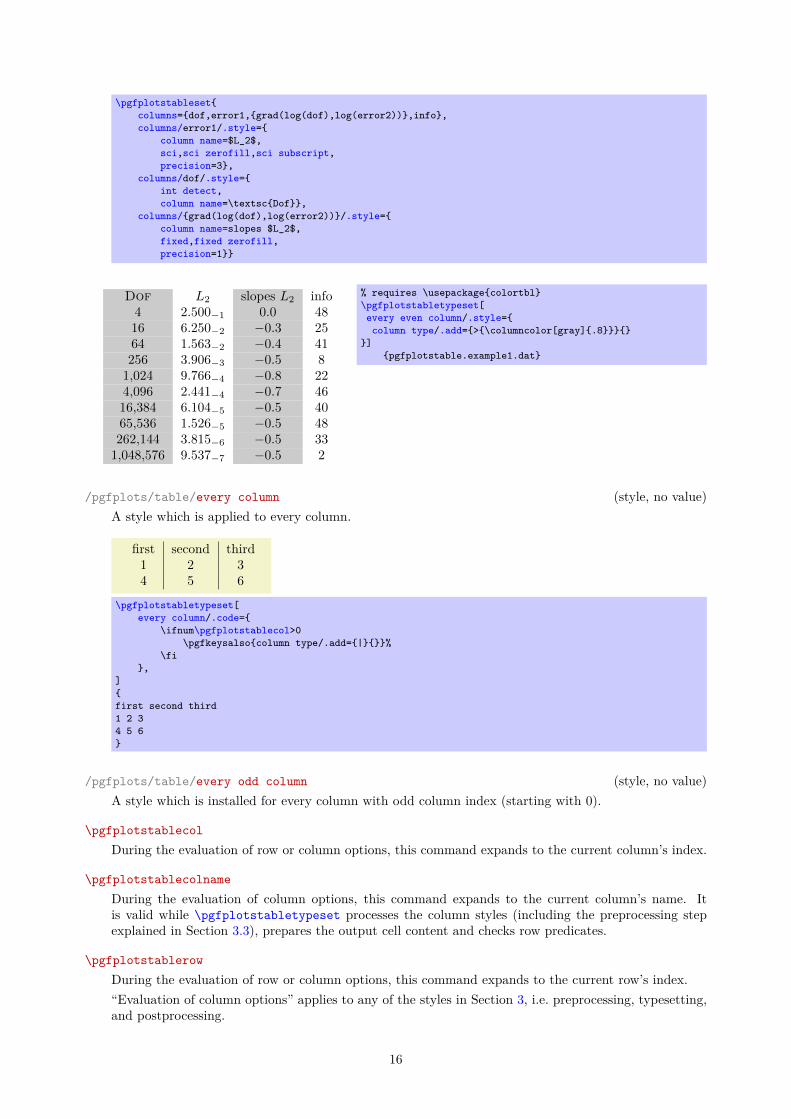
\pgfplotstableset{columns={dof,error1,{grad(log(dof),log(error2))},info},columns/error1/.style={



columns/{grad(log(dof),log(error2))}/.style={column name=slopes $L_2$,fixed,fixed zerofill,precision=1}}

Dof L2 slopes L2 info4 2.500−1 0.0 4816 6.250−2 −0.3 2564 1.563−2 −0.4 41256 3.906−3 −0.5 81,024 9.766−4 −0.8 224,096 2.441−4 −0.7 4616,384 6.104−5 −0.5 4065,536 1.526−5 −0.5 48262,144 3.815−6 −0.5 331,048,576 9.537−7 −0.5 2

% requires \usepackage{colortbl}\pgfplotstabletypeset[every even column/.style={column type/.add={>{\columncolor[gray]{.8}}}{}


/pgfplots/table/every column (style, no value)A style which is applied to every column.

first second third1 2 34 5 6

\pgfplotstabletypeset[every column/.code={

\ifnum\pgfplotstablecol>0\pgfkeysalso{column type/.add={|}{}}%

\fi},

]{first second third1 2 34 5 6}

/pgfplots/table/every odd column (style, no value)A style which is installed for every column with odd column index (starting with 0).

\pgfplotstablecolDuring the evaluation of row or column options, this command expands to the current column’s index.

\pgfplotstablecolnameDuring the evaluation of column options, this command expands to the current column’s name. Itis valid while \pgfplotstabletypeset processes the column styles (including the preprocessing stepexplained in Section 3.3), prepares the output cell content and checks row predicates.

\pgfplotstablerowDuring the evaluation of row or column options, this command expands to the current row’s index.“Evaluation of column options” applies to any of the styles in Section 3, i.e. preprocessing, typesetting,and postprocessing.

16

The macro \pgfplotstablerow can take any of the values 0, 1, 2, . . . , n − 1 where n is the value of\pgfplotstablerows.“Evaluation of row options” applies to stuff like every last row.Note that it will have the special value −1 for the header row.

\pgfplotstablecolsDuring the evaluation of row or column options, this command expands to the total number of columnsin the output table.

\pgfplotstablerowsDuring evaluation of columns, this command expands to the total number of input rows. You can useit inside of row predicate.During evaluation of rows, this command expands to the total number of output rows.

\pgfplotstablenameDuring \pgfplotstabletypeset, this macro contains the table’s macro name as top-level expansion. Ifyou are unfamiliar with “top-level-expansions” and ‘\expandafter’, you will probably never need thismacro.Advances users may benefit from expressions like\expandafter\pgfplotstabletypeset\pgfplotstablename.For tables which have been loaded from disk (and have no explicitly assigned macro name), this expandsto a temporary macro.

2.3 Configuring Row Appearance: StylesThe following styles allow to configure the final table code after any cell contents have been assigned.

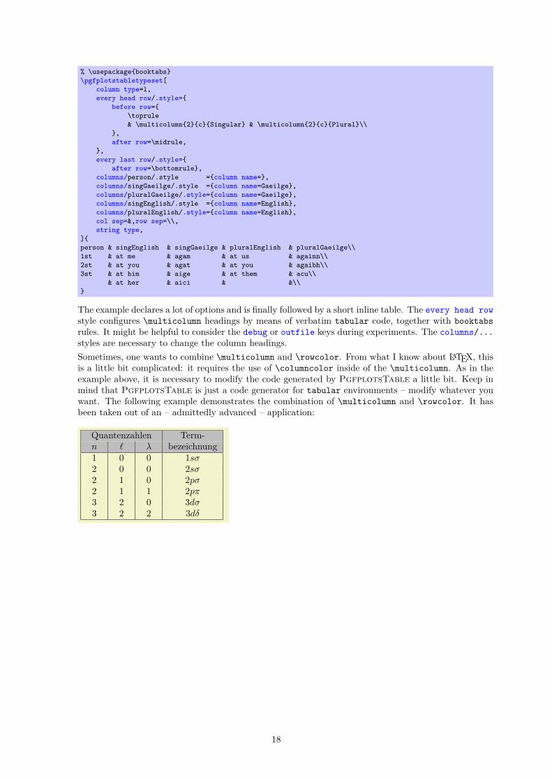
/pgfplots/table/before row={〈TEX code〉}Contains TEX code which will be installed before the first cell in a row.Keep in mind that PgfplotsTable does no magic – it is simply a code generator which producestabular environments. Consequently, you can add any TEX code which you would normally write intoyour tabular environment here.An example could be a multicolumn heading for which PgfplotsTable has no own solution:

Singular PluralEnglish Gaeilge English Gaeilge

1st at me agam at us againn2st at you agat at you agaibh3st at him aige at them acu

at her aici

17

% \usepackage{booktabs}\pgfplotstabletypeset[

column type=l,every head row/.style={

before row={\toprule& \multicolumn{2}{c}{Singular} & \multicolumn{2}{c}{Plural}\\

},after row=\midrule,

},every last row/.style={

after row=\bottomrule},columns/person/.style ={column name=},columns/singGaeilge/.style ={column name=Gaeilge},columns/pluralGaeilge/.style={column name=Gaeilge},columns/singEnglish/.style ={column name=English},columns/pluralEnglish/.style={column name=English},col sep=&,row sep=\\,string type,

]{person & singEnglish & singGaeilge & pluralEnglish & pluralGaeilge\\1st & at me & agam & at us & againn\\2st & at you & agat & at you & agaibh\\3st & at him & aige & at them & acu\\

& at her & aici & &\\}

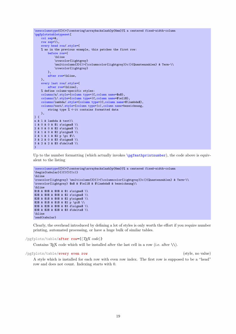
The example declares a lot of options and is finally followed by a short inline table. The every head rowstyle configures \multicolumn headings by means of verbatim tabular code, together with booktabsrules. It might be helpful to consider the debug or outfile keys during experiments. The columns/...styles are necessary to change the column headings.Sometimes, one wants to combine \multicolumn and \rowcolor. From what I know about LATEX, thisis a little bit complicated: it requires the use of \columncolor inside of the \multicolumn. As in theexample above, it is necessary to modify the code generated by PgfplotsTable a little bit. Keep inmind that PgfplotsTable is just a code generator for tabular environments – modify whatever youwant. The following example demonstrates the combination of \multicolumn and \rowcolor. It hasbeen taken out of an – admittedly advanced – application:

Quantenzahlen Term-n ` λ bezeichnung1 0 0 1sσ2 0 0 2sσ2 1 0 2pσ2 1 1 2pπ3 2 0 3dσ3 2 2 3dδ

18

\newcolumntype{C}{>{\centering\arraybackslash}p{6mm}}% a centered fixed-width-column\pgfplotstabletypeset[

col sep=&,row sep=\\,every head row/.style={% as in the previous example, this patches the first row:

before row={\hline\rowcolor{lightgray}\multicolumn{3}{|>{\columncolor{lightgray}}c|}{Quantenzahlen} & Term-\\\rowcolor{lightgray}

},after row=\hline,

},every last row/.style={

after row=\hline},% define column-specific styles:columns/n/.style={column type=|C,column name=$n$},columns/l/.style={column type=|C,column name=$\ell$},columns/lambda/.style={column type=|C,column name=$\lambda$},columns/text/.style={column type=|c|,column name=bezeichnung,

string type % <-it contains formatted data},

] {n & l & lambda & text\\1 & 0 & 0 & $1 s\sigma$ \\2 & 0 & 0 & $2 s\sigma$ \\2 & 1 & 0 & $2 p\sigma$ \\2 & 1 & 1 & $2 p \pi $\\3 & 2 & 0 & $3 d\sigma$ \\3 & 2 & 2 & $3 d\delta$ \\}

Up to the number formatting (which actually invokes \pgfmathprintnumber), the code above is equiv-alent to the listing

\newcolumntype{C}{>{\centering\arraybackslash}p{6mm}}% a centered fixed-width-column\begin{tabular}{|C|C|C|c|}\hline\rowcolor{lightgray} \multicolumn{3}{|>{\columncolor{lightgray}}c|}{Quantenzahlen} & Term-\\\rowcolor{lightgray} $n$ & $\ell$ & $\lambda$ & bezeichnung\\\hline$1$ & $0$ & $0$ & $1 s\sigma$ \\$2$ & $0$ & $0$ & $2 s\sigma$ \\$2$ & $1$ & $0$ & $2 p\sigma$ \\$2$ & $1$ & $1$ & $2 p \pi$ \\$3$ & $2$ & $0$ & $3 d\sigma$ \\$3$ & $2$ & $2$ & $3 d\delta$ \\\hline\end{tabular}

Clearly, the overhead introduced by defining a lot of styles is only worth the effort if you require numberprinting, automated processing, or have a huge bulk of similar tables.

/pgfplots/table/after row={〈TEX code〉}Contains TEX code which will be installed after the last cell in a row (i.e. after \\).

/pgfplots/table/every even row (style, no value)A style which is installed for each row with even row index. The first row is supposed to be a “head”row and does not count. Indexing starts with 0.

19

\pgfplotstableset{columns={dof,error1,{grad(log(dof),log(error2))}},columns/error1/.style={



columns/{grad(log(dof),log(error2))}/.style={column name=slopes $L_2$,fixed,fixed zerofill,precision=1}}

Dof L2 slopes L2

4 2.500−1 0.016 6.250−2 −0.364 1.563−2 −0.4256 3.906−3 −0.51,024 9.766−4 −0.84,096 2.441−4 −0.716,384 6.104−5 −0.565,536 1.526−5 −0.5262,144 3.815−6 −0.51,048,576 9.537−7 −0.5

% requires \usepackage{booktabs}\pgfplotstabletypeset[

every head row/.style={before row=\toprule,after row=\midrule},

every last row/.style={after row=\bottomrule},


Dof L2 slopes L2

4 2.500−1 0.016 6.250−2 −0.364 1.563−2 −0.4256 3.906−3 −0.51,024 9.766−4 −0.84,096 2.441−4 −0.716,384 6.104−5 −0.565,536 1.526−5 −0.5262,144 3.815−6 −0.51,048,576 9.537−7 −0.5

% requires \usepackage{booktabs,colortbl}\pgfplotstabletypeset[

every even row/.style={before row={\rowcolor[gray]{0.9}}},




/pgfplots/table/every odd row (style, no value)A style which is installed for each row with odd row index. The first row is supposed to be a “head”row and does not count. Indexing starts with 0.

/pgfplots/table/every head row (style, no value)A style which is installed for each first row in the tabular. This can be used to adjust options for columnnames or to add extra lines/colors.

Col A B CThe first column E F

20

\pgfplotstabletypeset[% suppress the header row 'col1 col2 col3':every head row/.style={output empty row},col sep=comma,columns/col1/.style={string type,column type=r},columns/col2/.style={string type,column type=l},columns/col3/.style={string type,column type=l},]

{col1,col2,col3Col A,B,CThe first column,E,F

}

/pgfplots/table/every first row (style, no value)A style which is installed for each first data row, i.e. after the head row.

/pgfplots/table/every last row (style, no value)A style which is installed for each last row.

/pgfplots/table/every row no 〈index〉 (style, no value)A style which is installed for the row with index 〈index〉.

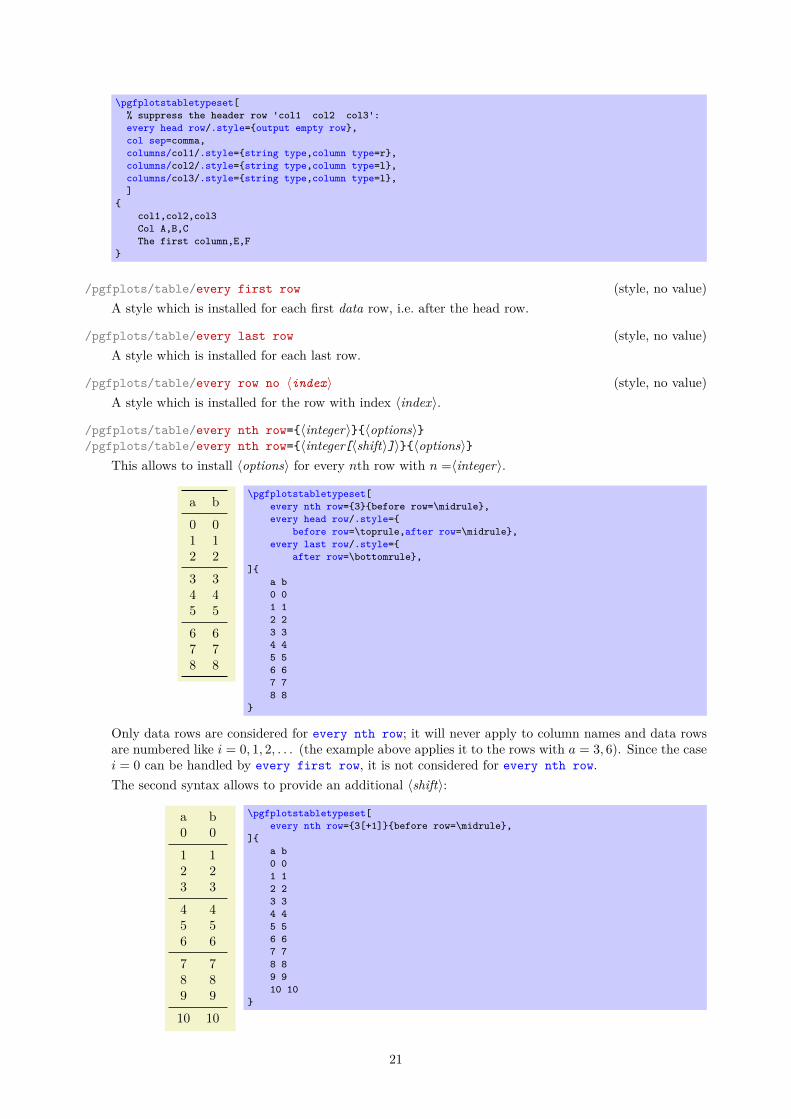
/pgfplots/table/every nth row={〈integer〉}{〈options〉}/pgfplots/table/every nth row={〈integer[〈shift〉]〉}{〈options〉}

This allows to install 〈options〉 for every nth row with n =〈integer〉.

a b0 01 12 2

3 34 45 5

6 67 78 8

\pgfplotstabletypeset[every nth row={3}{before row=\midrule},every head row/.style={

before row=\toprule,after row=\midrule},every last row/.style={

after row=\bottomrule},]{

a b0 01 12 23 34 45 56 67 78 8

}

Only data rows are considered for every nth row; it will never apply to column names and data rowsare numbered like i = 0, 1, 2, . . . (the example above applies it to the rows with a = 3, 6). Since the casei = 0 can be handled by every first row, it is not considered for every nth row.The second syntax allows to provide an additional 〈shift〉:

a b0 0

1 12 23 3

4 45 56 6

7 78 89 9

10 10

\pgfplotstabletypeset[every nth row={3[+1]}{before row=\midrule},

]{a b0 01 12 23 34 45 56 67 78 89 910 10

}

21

Here, the style is applied to rows i = 1, 4, 7, 10 (mathematically, it is applied if (i mod n) =〈shift〉).The 〈shift〉 can be negative.You can define many every nth row styles, they are processed in the order of occurrence (considerusing before row/.add={〈before existing〉}{〈after existing〉} to modify an existing value).Note that every nth row/.style 2 args=... is the same as every nth row=....

/pgfplots/table/output empty row (style, no value)A style which suppresses output for the current row.This style is evaluated very late, after all column-specific content modifications have been applied. It isequivalent to

\pgfplotstableset{output empty row/.style={

typeset cell/.style={@cell content={}}},

}

See every head row for an application.

2.4 Configuring Single Cell Appearance: StylesBesides the possibilities to change column styles and row styles, there are also a couple of styles to changesingle cells.

/pgfplots/table/every row 〈rowindex〉 column 〈colindex〉 (style, no value)A style which applies to at most one cell: the one with row index 〈rowindex〉 and column index 〈colindex〉.Each of these indices starts with 0.The style is evaluated in the same context as the preproc cell content, assign cell content, andpostproc cell content keys and it is a legitimate possibility to modify any of these parameters. It isalso possible to replace the initial cell value by assigning something to @cell content.For example, consider this unmodified table:

colA colB colC11 12 1321 22 23

\pgfplotstabletypeset[col sep=&,row sep=\\]{

colA & colB & colC \\11 & 12 & 13 \\21 & 22 & 23 \\

}

Now, we change the number format of one of its cells, and at the same time we change the formattingof another (single) cell:

colA colB colC11 12 1321 22 2.3 · 101

\pgfplotstabletypeset[every row 1 column 2/.style={/pgf/number format/sci},every row 0 column 0/.style={postproc cell content/.style={@cell content=\textbf{##1}}},col sep=&,row sep=\\]{

colA & colB & colC \\11 & 12 & 13 \\21 & 22 & 23 \\

}

Note that this style is (only) applied to input row/column values.

/pgfplots/table/every row no 〈rowindex〉 column no 〈colindex〉 (style, no value)This is actually the same – row no and row are both supported, the same for column and column no.

/pgfplots/table/every row 〈rowindex〉 column 〈colname〉 (style, no value)A similar style as above, but it allows column names rather than column indices. Column names needto be provided in the same way as for other column-specific styles (including the extra curly braces incase 〈colname〉 contains special characters).

22

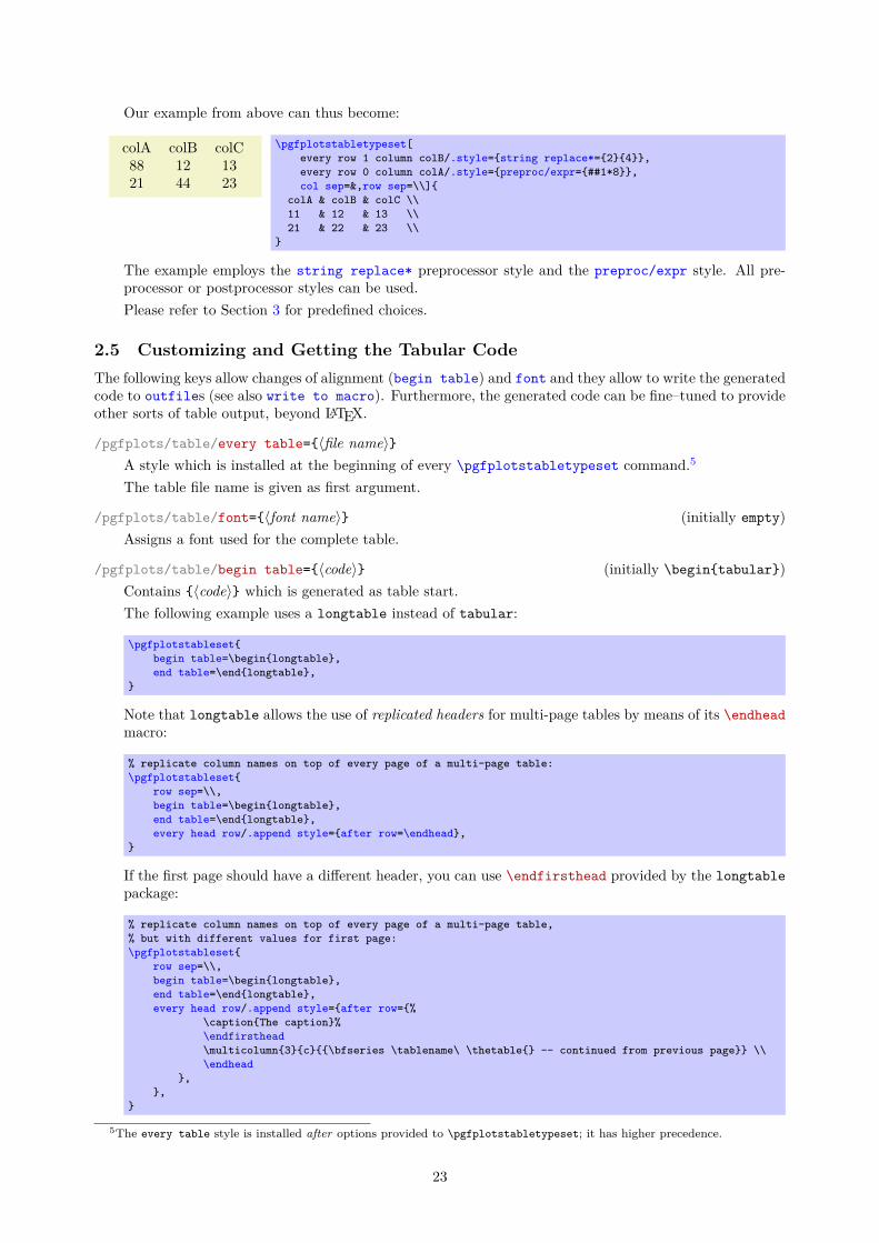
Our example from above can thus become:


\pgfplotstabletypeset[every row 1 column colB/.style={string replace*={2}{4}},every row 0 column colA/.style={preproc/expr={##1*8}},col sep=&,row sep=\\]{

colA & colB & colC \\11 & 12 & 13 \\21 & 22 & 23 \\

}

The example employs the string replace* preprocessor style and the preproc/expr style. All pre-processor or postprocessor styles can be used.Please refer to Section 3 for predefined choices.

2.5 Customizing and Getting the Tabular CodeThe following keys allow changes of alignment (begin table) and font and they allow to write the generatedcode to outfiles (see also write to macro). Furthermore, the generated code can be fine–tuned to provideother sorts of table output, beyond LATEX.

/pgfplots/table/every table={〈file name〉}A style which is installed at the beginning of every \pgfplotstabletypeset command.5

The table file name is given as first argument.

/pgfplots/table/font={〈font name〉} (initially empty)Assigns a font used for the complete table.

/pgfplots/table/begin table={〈code〉} (initially \begin{tabular})Contains {〈code〉} which is generated as table start.The following example uses a longtable instead of tabular:

\pgfplotstableset{begin table=\begin{longtable},end table=\end{longtable},

}

Note that longtable allows the use of replicated headers for multi-page tables by means of its \endheadmacro:

% replicate column names on top of every page of a multi-page table:\pgfplotstableset{

row sep=\\,begin table=\begin{longtable},end table=\end{longtable},every head row/.append style={after row=\endhead},

}

If the first page should have a different header, you can use \endfirsthead provided by the longtablepackage:

% replicate column names on top of every page of a multi-page table,% but with different values for first page:\pgfplotstableset{

row sep=\\,begin table=\begin{longtable},end table=\end{longtable},every head row/.append style={after row={%

\caption{The caption}%\endfirsthead\multicolumn{3}{c}{{\bfseries \tablename\ \thetable{} -- continued from previous page}} \\\endhead

},},

}

5The every table style is installed after options provided to \pgfplotstabletypeset; it has higher precedence.

23

The preceding example uses the longtable macros \caption, \endfirsthead, \thetable, and\endhead. In addition, it requires to provide the number of columns ({3} in this case) explicitly.It is also possible to change the value of begin table. For example,

\pgfplotstableset{begin table/.add={}{[t]},

}

prepends the empty string {} and appends the prefix [t]. Thus, ‘\begin{tabular}’ becomes‘\begin{tabular}[t]’.

/pgfplots/table/end table={〈code〉} (initially \end{tabular})Contains 〈code〉 which is generated as table end.

/pgfplots/table/typeset cell/.code={〈...〉}A code key which assigns /pgfplots/table/@cell content to the final output of the current cell.The first argument, #1, is the final cell’s value. After this macro, the value of @cell content will bewritten to the output.The default implementation is

/pgfplots/table/typeset cell/.code={%\ifnum\c@pgfplotstable@colindex=\c@pgfplotstable@numcols\relax

\pgfkeyssetvalue{/pgfplots/table/@cell content}{#1\\}%\else

\pgfkeyssetvalue{/pgfplots/table/@cell content}{#1&}%\fi

},

Attention: The value of \pgfplotstablecol starts with 1 in this context, i.e. it is in the range1, . . . , n where n = \pgfplotstablecols. This simplifies checks whether we have the last column.

/pgfplots/table/outfile={〈file name〉} (initially empty)Writes the generated tabular code into 〈file name〉. It can then be used with \input{〈file name〉},PgfplotsTable is no longer required since it contains a completely normal tabular.

dof error14 0.2516 6.25 · 10−2

64 1.56 · 10−2

256 3.91 · 10−3

1,024 9.77 · 10−4

4,096 2.44 · 10−4

16,384 6.1 · 10−5

65,536 1.53 · 10−5

2.62 · 105 3.81 · 10−6

1.05 · 106 9.54 · 10−7

\pgfplotstabletypeset[columns={dof,error1},outfile=pgfplotstable.example1.out.tex]{pgfplotstable.example1.dat}

and pgfplotstable.example1.out.tex contains\begin {tabular}{cc}%dof&error1\\%\pgfutilensuremath {4}&\pgfutilensuremath {0.25}\\%\pgfutilensuremath {16}&\pgfutilensuremath {6.25\cdot 10^{-2}}\\%\pgfutilensuremath {64}&\pgfutilensuremath {1.56\cdot 10^{-2}}\\%\pgfutilensuremath {256}&\pgfutilensuremath {3.91\cdot 10^{-3}}\\%\pgfutilensuremath {1{,}024}&\pgfutilensuremath {9.77\cdot 10^{-4}}\\%\pgfutilensuremath {4{,}096}&\pgfutilensuremath {2.44\cdot 10^{-4}}\\%\pgfutilensuremath {16{,}384}&\pgfutilensuremath {6.1\cdot 10^{-5}}\\%

24

\pgfutilensuremath {65{,}536}&\pgfutilensuremath {1.53\cdot 10^{-5}}\\%\pgfutilensuremath {2.62\cdot 10^{5}}&\pgfutilensuremath {3.81\cdot 10^{-6}}\\%\pgfutilensuremath {1.05\cdot 10^{6}}&\pgfutilensuremath {9.54\cdot 10^{-7}}\\%\end {tabular}%

The command \pgfutilensuremath checks whether math mode is active and switches to math modeif necessary.6

/pgfplots/table/include outfiles={〈boolean〉} (initially false)If enabled, any already existing outfile will be \input instead of overwritten.

\pgfplotstableset{include outfiles} % for example in the document's preamble

This allows to place any corrections manually into generated output files since PgfplotsTable won’toverwrite the resulting tables automatically.This will affect tables for which the outfile option is set. If you wish to apply it to every table, consider

\pgfplotstableset{every table/.append style={outfile={#1.out}}}

which will generate an outfile name for every table.

/pgfplots/table/force remake={〈boolean〉} (initially false)If enabled, the effect of include outfiles is disabled. As all key settings only last until the next brace(or \end〈〉), this key can be used to regenerate some output files while others are still included.

/pgfplots/table/write to macro={〈\macroname〉}If the value of write to macro is not empty, the completely generated (tabular) code will be writteninto the macro 〈\macroname〉.See the typeset=false key in case you need only the resulting macro.

/pgfplots/table/skip coltypes=true|false (initially false)Allows to skip the 〈coltypes〉 in \begin{tabular}{〈coltypes〉}. This allows simplifications for other tabletypes which don’t have LATEX’s table format.

/pgfplots/table/typeset=true|false (initially true)A boolean which disables the final typesetting stage. Use typeset=false in conjunction with writeto macro if only the generated code is of interest and TEX should not attempt to produce any contentin the output pdf.

/pgfplots/table/debug={〈boolean〉} (initially false)If enabled, it will write every final tabular code to your logfile.

/pgfplots/table/TeX comment={〈comment sign〉} (initially %)The comment sign which is inserted into outfiles to suppress trailing white space.

As a last example, we use PgfplotsTable to write an .html file (including number formatting and round-ing!):

<table><tr><td>level</td><td>dof</td><td>error1</td></tr><tr><td>1</td><td>4</td><td>0.25</td></tr><tr><td>2</td><td>16</td><td>6.25e-2</td></tr><tr><td>3</td><td>64</td><td>1.56e-2</td></tr><tr><td>4</td><td>256</td><td>3.91e-3</td></tr><tr><td>5</td><td>1024</td><td>9.77e-4</td></tr><tr><td>6</td><td>4096</td><td>2.44e-4</td></tr><tr><td>7</td><td>16384</td><td>6.1e-5</td></tr><tr><td>8</td><td>65536</td><td>1.53e-5</td></tr><tr><td>9</td><td>2.62e5</td><td>3.81e-6</td></tr><tr><td>10</td><td>1.05e6</td><td>9.54e-7</td></tr></table>

6Please note that \pgfutilensuremath needs to be replaced by \ensuremath if you want to use the output file independentof pgf. That can be done by \let\pgfutilensuremath=\ensuremath which enables the LATEX command \ensuremath.

25

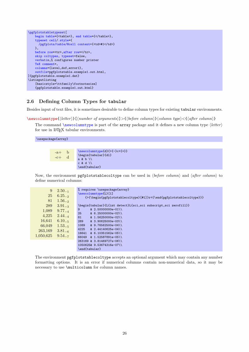
\pgfplotstabletypeset[begin table={<table>}, end table={</table>},typeset cell/.style={

/pgfplots/table/@cell content={<td>#1</td>}},before row=<tr>,after row=</tr>,skip coltypes, typeset=false,verbatim,% configures number printerTeX comment=,columns={level,dof,error1},outfile=pgfplotstable.example1.out.html,

]{pgfplotstable.example1.dat}\lstinputlisting

[basicstyle=\ttfamily\footnotesize]{pgfplotstable.example1.out.html}

2.6 Defining Column Types for tabular

Besides input of text files, it is sometimes desirable to define column types for existing tabular environments.

\newcolumntype{〈letter〉}[〈number of arguments〉]>{〈before column〉}〈column type〉<{〈after column〉}The command \newcolumntype is part of the array package and it defines a new column type 〈letter〉for use in LATEX tabular environments.

\usepackage{array}

-a+ b-c+ d

\newcolumntype{d}{>{-}c<{+}}\begin{tabular}{dl}a & b \\c & d \\\end{tabular}

Now, the environment pgfplotstablecoltype can be used in 〈before column〉 and 〈after column〉 todefine numerical columns:

9 2.50−1

25 6.25−2

81 1.56−2

289 3.91−3

1,089 9.77−4

4,225 2.44−4

16,641 6.10−5

66,049 1.53−5

263,169 3.81−6

1,050,625 9.54−7

% requires \usepackage{array}\newcolumntype{L}[1]

{>{\begin{pgfplotstablecoltype}[#1]}r<{\end{pgfplotstablecoltype}}}

\begin{tabular}{L{int detect}L{sci,sci subscript,sci zerofill}}9 & 2.50000000e-01\\25 & 6.25000000e-02\\81 & 1.56250000e-02\\289 & 3.90625000e-03\\1089 & 9.76562500e-04\\4225 & 2.44140625e-04\\16641 & 6.10351562e-05\\66049 & 1.52587891e-05\\263169 & 3.81469727e-06\\1050625& 9.53674316e-07\\\end{tabular}

The environment pgfplotstablecoltype accepts an optional argument which may contain any numberformatting options. It is an error if numerical columns contain non-numerical data, so it may benecessary to use \multicolumn for column names.

26

Dof Error9 2.50−1

25 6.25−2

81 1.56−2

289 3.91−3

1,089 9.77−4

4,225 2.44−4

16,641 6.10−5

66,049 1.53−5

263,169 3.81−6

1,050,625 9.54−7

% requires \usepackage{array}\newcolumntype{L}[1]

{>{\begin{pgfplotstablecoltype}[#1]}r<{\end{pgfplotstablecoltype}}}

\begin{tabular}{L{int detect}L{sci,sci subscript,sci zerofill}}\multicolumn{1}{r}{Dof} & \multicolumn{1}{r}{Error}\\9 & 2.50000000e-01\\25 & 6.25000000e-02\\81 & 1.56250000e-02\\289 & 3.90625000e-03\\1089 & 9.76562500e-04\\4225 & 2.44140625e-04\\16641 & 6.10351562e-05\\66049 & 1.52587891e-05\\263169 & 3.81469727e-06\\1050625& 9.53674316e-07\\\end{tabular}

2.7 Number Formatting OptionsThe following extract of [2] explains how to configure number formats. The common option prefix/pgf/number format can be omitted; it will be recognized automatically.

All these number formatting options can also be applied to pgfplots.

\pgfmathprintnumber{〈x〉}Generates pretty-printed output for the (real) number 〈x〉. The input number 〈x〉 is parsed using\pgfmathfloatparsenumber which allows arbitrary precision.Numbers are typeset in math mode using the current set of number printing options, see below. Optionalarguments can also be provided using \pgfmathprintnumber[〈options〉]{〈x〉}.

\pgfmathprintnumberto{〈x〉}{〈\macro〉}Returns the resulting number into 〈\macro〉 instead of typesetting it directly.

/pgf/number format/fixed (no value)Configures \pgfmathprintnumber to round the number to a fixed number of digits after the period,discarding any trailing zeros.

4.57 0 0.1 24,415.98 123,456.12

\pgfkeys{/pgf/number format/.cd,fixed,precision=2}\pgfmathprintnumber{4.568}\hspace{1em}\pgfmathprintnumber{5e-04}\hspace{1em}\pgfmathprintnumber{0.1}\hspace{1em}\pgfmathprintnumber{24415.98123}\hspace{1em}\pgfmathprintnumber{123456.12345}

See Section 2.7.1 for how to change the appearance.

/pgf/number format/fixed zerofill={〈boolean〉} (default true)Enables or disables zero filling for any number drawn in fixed point format.

4.57 0.00 0.10 24,415.98 123,456.12

\pgfkeys{/pgf/number format/.cd,fixed,fixed zerofill,precision=2}\pgfmathprintnumber{4.568}\hspace{1em}\pgfmathprintnumber{5e-04}\hspace{1em}\pgfmathprintnumber{0.1}\hspace{1em}\pgfmathprintnumber{24415.98123}\hspace{1em}\pgfmathprintnumber{123456.12345}

This key affects numbers drawn with fixed or std styles (the latter only if no scientific format ischosen).

4.57 5 · 10−5 1.00 1.23 · 105

27

\pgfkeys{/pgf/number format/.cd,std,fixed zerofill,precision=2}\pgfmathprintnumber{4.568}\hspace{1em}\pgfmathprintnumber{5e-05}\hspace{1em}\pgfmathprintnumber{1}\hspace{1em}\pgfmathprintnumber{123456.12345}

See Section 2.7.1 for how to change the appearance.

/pgf/number format/sci (no value)Configures \pgfmathprintnumber to display numbers in scientific format, that means sign, mantissaand exponent (base 10). The mantissa is rounded to the desired precision (or sci precision, seebelow).

4.57 · 100 5 · 10−4 1 · 10−1 2.44 · 104 1.23 · 105

\pgfkeys{/pgf/number format/.cd,sci,precision=2}\pgfmathprintnumber{4.568}\hspace{1em}\pgfmathprintnumber{5e-04}\hspace{1em}\pgfmathprintnumber{0.1}\hspace{1em}\pgfmathprintnumber{24415.98123}\hspace{1em}\pgfmathprintnumber{123456.12345}

See Section 2.7.1 for how to change the exponential display style.

/pgf/number format/sci zerofill={〈boolean〉} (default true)Enables or disables zero filling for any number drawn in scientific format.

4.57 · 100 5.00 · 10−4 1.00 · 10−1 2.44 · 104 1.23 · 105

\pgfkeys{/pgf/number format/.cd,sci,sci zerofill,precision=2}\pgfmathprintnumber{4.568}\hspace{1em}\pgfmathprintnumber{5e-04}\hspace{1em}\pgfmathprintnumber{0.1}\hspace{1em}\pgfmathprintnumber{24415.98123}\hspace{1em}\pgfmathprintnumber{123456.12345}

As with fixed zerofill, this option does only affect numbers drawn in sci format (or std if thescientific format is chosen).See Section 2.7.1 for how to change the exponential display style.

/pgf/number format/zerofill={〈boolean〉} (style, default true)Sets both fixed zerofill and sci zerofill at once.

/pgf/number format/std (no value)/pgf/number format/std=〈lower e〉/pgf/number format/std=〈lower e〉:〈upper e〉

Configures \pgfmathprintnumber to a standard algorithm. It chooses either fixed or sci, dependingon the order of magnitude. Let n = s · m · 10e be the input number and p the current precision. If−p/2 ≤ e ≤ 4, the number is displayed using fixed format. Otherwise, it is displayed using sci format.

4.57 5 · 10−4 0.1 24,415.98 1.23 · 105

\pgfkeys{/pgf/number format/.cd,std,precision=2}\pgfmathprintnumber{4.568}\hspace{1em}\pgfmathprintnumber{5e-04}\hspace{1em}\pgfmathprintnumber{0.1}\hspace{1em}\pgfmathprintnumber{24415.98123}\hspace{1em}\pgfmathprintnumber{123456.12345}

The parameters can be customized using the optional integer argument(s): if 〈lower e〉 ≤ e ≤ 〈upper e〉,the number is displayed in fixed format, otherwise in sci format. Note that 〈lower e〉 should benegative for useful results. The precision used for scientific format can be adjusted with sci precisionif necessary.

28

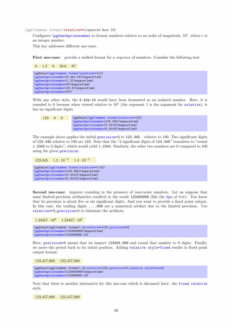
/pgf/number format/relative*=〈exponent base 10〉Configures \pgfmathprintnumber to format numbers relative to an order of magnitude, 10r, where r isan integer number.This key addresses different use-cases.

First use-case: provide a unified format for a sequence of numbers. Consider the following test:

0 1.2 6 20.6 87

\pgfkeys{/pgf/number format/relative*={1}}\pgfmathprintnumber{6.42e-16}\hspace{1em}\pgfmathprintnumber{1.2}\hspace{1em}\pgfmathprintnumber{6}\hspace{1em}\pgfmathprintnumber{20.6}\hspace{1em}\pgfmathprintnumber{87}

With any other style, the 6.42e-16 would have been formatted as an isolated number. Here, it isrounded to 0 because when viewed relative to 101 (the exponent 1 is the argument for relative), ithas no significant digits.

123 0 0 \pgfkeys{/pgf/number format/relative*={2}}\pgfmathprintnumber{123.345}\hspace{1em}\pgfmathprintnumber{0.0012}\hspace{1em}\pgfmathprintnumber{0.0014}\hspace{1em}

The example above applies the initial precision=2 to 123.345 – relative to 100. Two significant digitsof 123.345 relative to 100 are 123. Note that the “2 significant digits of 123.345” translates to “round1.2345 to 2 digits”, which would yield 1.2300. Similarly, the other two numbers are 0 compared to 100using the given precision.

123.345 1.2 · 10−3 1.4 · 10−3

\pgfkeys{/pgf/number format/relative*={-3}}\pgfmathprintnumber{123.345}\hspace{1em}\pgfmathprintnumber{0.0012}\hspace{1em}\pgfmathprintnumber{0.0014}\hspace{1em}

Second use-case: improve rounding in the presence of inaccurate numbers. Let us suppose thatsome limited-precision arithmetics resulted in the result 123456999 (like the fpu of pgf). You knowthat its precision is about five or six significant digits. And you want to provide a fixed point output.In this case, the trailing digits ....999 are a numerical artifact due to the limited precision. Userelative*=3,precision=0 to eliminate the artifacts:

1.23457 · 108 1.23457 · 108

\pgfkeys{/pgf/number format/.cd,relative*={3},precision=0}\pgfmathprintnumber{123456999}\hspace{1em}\pgfmathprintnumber{123456999.12}

Here, precision=0 means that we inspect 123456.999 and round that number to 0 digits. Finally,we move the period back to its initial position. Adding relative style=fixed results in fixed pointoutput format:

123,457,000 123,457,000

\pgfkeys{/pgf/number format/.cd,relative*={3},precision=0,relative style=fixed}\pgfmathprintnumber{123456999}\hspace{1em}\pgfmathprintnumber{123456999.12}

Note that there is another alternative for this use-case which is discussed later: the fixed relativestyle.

123,457,000 123,457,000

29

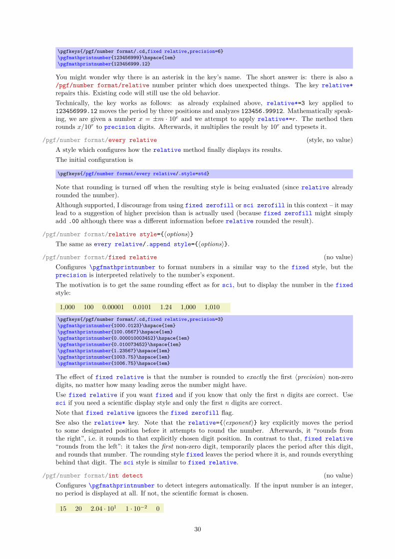
\pgfkeys{/pgf/number format/.cd,fixed relative,precision=6}\pgfmathprintnumber{123456999}\hspace{1em}\pgfmathprintnumber{123456999.12}

You might wonder why there is an asterisk in the key’s name. The short answer is: there is also a/pgf/number format/relative number printer which does unexpected things. The key relative*repairs this. Existing code will still use the old behavior.Technically, the key works as follows: as already explained above, relative*=3 key applied to123456999.12 moves the period by three positions and analyzes 123456.99912. Mathematically speak-ing, we are given a number x = ±m · 10e and we attempt to apply relative*=r. The method thenrounds x/10r to precision digits. Afterwards, it multiplies the result by 10r and typesets it.

/pgf/number format/every relative (style, no value)A style which configures how the relative method finally displays its results.The initial configuration is

\pgfkeys{/pgf/number format/every relative/.style=std}

Note that rounding is turned off when the resulting style is being evaluated (since relative alreadyrounded the number).Although supported, I discourage from using fixed zerofill or sci zerofill in this context – it maylead to a suggestion of higher precision than is actually used (because fixed zerofill might simplyadd .00 although there was a different information before relative rounded the result).

/pgf/number format/relative style={〈options〉}The same as every relative/.append style={〈options〉}.

/pgf/number format/fixed relative (no value)Configures \pgfmathprintnumber to format numbers in a similar way to the fixed style, but theprecision is interpreted relatively to the number’s exponent.The motivation is to get the same rounding effect as for sci, but to display the number in the fixedstyle:

1,000 100 0.00001 0.0101 1.24 1,000 1,010

\pgfkeys{/pgf/number format/.cd,fixed relative,precision=3}\pgfmathprintnumber{1000.0123}\hspace{1em}\pgfmathprintnumber{100.0567}\hspace{1em}\pgfmathprintnumber{0.000010003452}\hspace{1em}\pgfmathprintnumber{0.010073452}\hspace{1em}\pgfmathprintnumber{1.23567}\hspace{1em}\pgfmathprintnumber{1003.75}\hspace{1em}\pgfmathprintnumber{1006.75}\hspace{1em}

The effect of fixed relative is that the number is rounded to exactly the first 〈precision〉 non-zerodigits, no matter how many leading zeros the number might have.Use fixed relative if you want fixed and if you know that only the first n digits are correct. Usesci if you need a scientific display style and only the first n digits are correct.Note that fixed relative ignores the fixed zerofill flag.See also the relative* key. Note that the relative={〈exponent〉} key explicitly moves the periodto some designated position before it attempts to round the number. Afterwards, it “rounds fromthe right”, i.e. it rounds to that explicitly chosen digit position. In contrast to that, fixed relative“rounds from the left”: it takes the first non-zero digit, temporarily places the period after this digit,and rounds that number. The rounding style fixed leaves the period where it is, and rounds everythingbehind that digit. The sci style is similar to fixed relative.

/pgf/number format/int detect (no value)Configures \pgfmathprintnumber to detect integers automatically. If the input number is an integer,no period is displayed at all. If not, the scientific format is chosen.

15 20 2.04 · 101 1 · 10−2 0

30

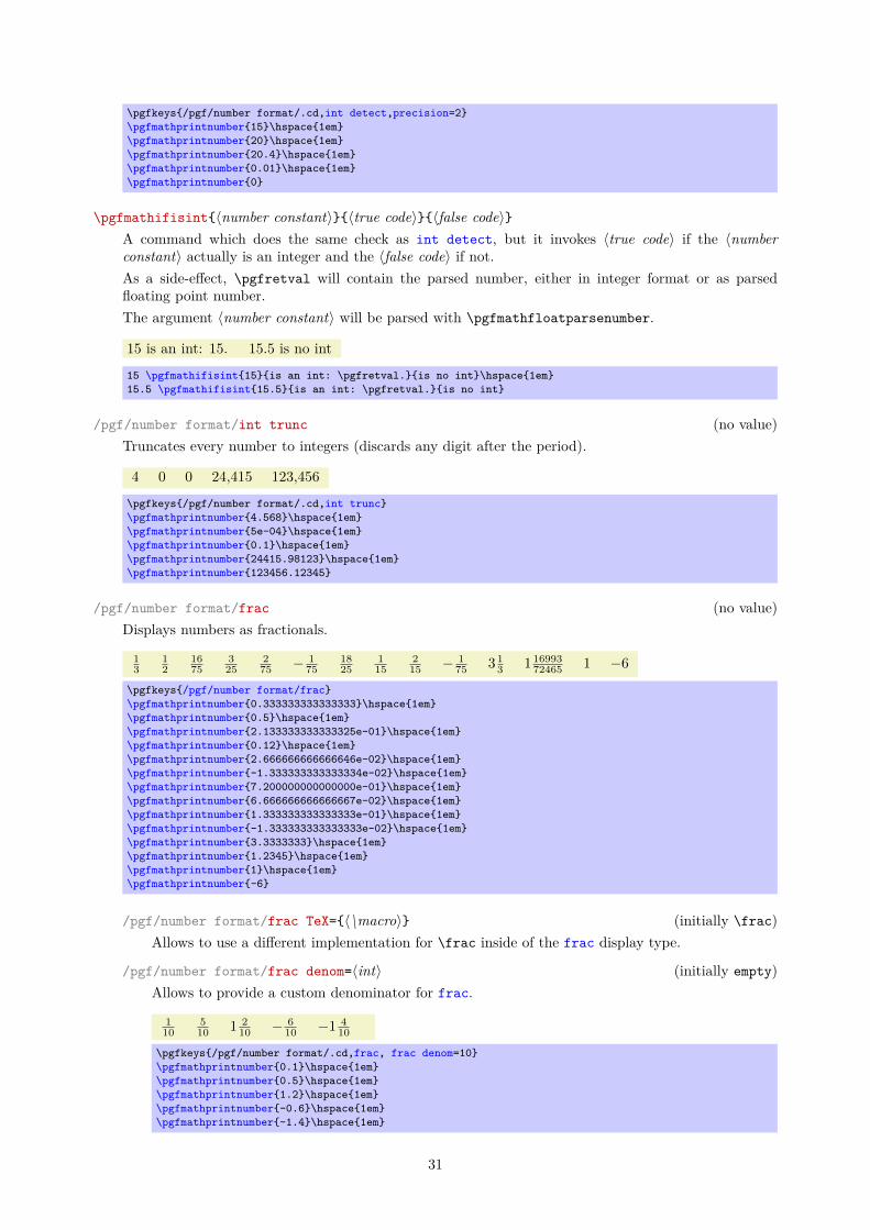
\pgfkeys{/pgf/number format/.cd,int detect,precision=2}\pgfmathprintnumber{15}\hspace{1em}\pgfmathprintnumber{20}\hspace{1em}\pgfmathprintnumber{20.4}\hspace{1em}\pgfmathprintnumber{0.01}\hspace{1em}\pgfmathprintnumber{0}

\pgfmathifisint{〈number constant〉}{〈true code〉}{〈false code〉}A command which does the same check as int detect, but it invokes 〈true code〉 if the 〈numberconstant〉 actually is an integer and the 〈false code〉 if not.As a side-effect, \pgfretval will contain the parsed number, either in integer format or as parsedfloating point number.The argument 〈number constant〉 will be parsed with \pgfmathfloatparsenumber.

15 is an int: 15. 15.5 is no int

15 \pgfmathifisint{15}{is an int: \pgfretval.}{is no int}\hspace{1em}15.5 \pgfmathifisint{15.5}{is an int: \pgfretval.}{is no int}

/pgf/number format/int trunc (no value)Truncates every number to integers (discards any digit after the period).

4 0 0 24,415 123,456

\pgfkeys{/pgf/number format/.cd,int trunc}\pgfmathprintnumber{4.568}\hspace{1em}\pgfmathprintnumber{5e-04}\hspace{1em}\pgfmathprintnumber{0.1}\hspace{1em}\pgfmathprintnumber{24415.98123}\hspace{1em}\pgfmathprintnumber{123456.12345}

/pgf/number format/frac (no value)Displays numbers as fractionals.

13

12

1675

325

275 − 1

751825

115

215 − 1

75 3 13 1 16993

72465 1 −6

\pgfkeys{/pgf/number format/frac}\pgfmathprintnumber{0.333333333333333}\hspace{1em}\pgfmathprintnumber{0.5}\hspace{1em}\pgfmathprintnumber{2.133333333333325e-01}\hspace{1em}\pgfmathprintnumber{0.12}\hspace{1em}\pgfmathprintnumber{2.666666666666646e-02}\hspace{1em}\pgfmathprintnumber{-1.333333333333334e-02}\hspace{1em}\pgfmathprintnumber{7.200000000000000e-01}\hspace{1em}\pgfmathprintnumber{6.666666666666667e-02}\hspace{1em}\pgfmathprintnumber{1.333333333333333e-01}\hspace{1em}\pgfmathprintnumber{-1.333333333333333e-02}\hspace{1em}\pgfmathprintnumber{3.3333333}\hspace{1em}\pgfmathprintnumber{1.2345}\hspace{1em}\pgfmathprintnumber{1}\hspace{1em}\pgfmathprintnumber{-6}

/pgf/number format/frac TeX={〈\macro〉} (initially \frac)Allows to use a different implementation for \frac inside of the frac display type.

/pgf/number format/frac denom=〈int〉 (initially empty)Allows to provide a custom denominator for frac.

110

510 1 2

10 − 610 −1 4

10

\pgfkeys{/pgf/number format/.cd,frac, frac denom=10}\pgfmathprintnumber{0.1}\hspace{1em}\pgfmathprintnumber{0.5}\hspace{1em}\pgfmathprintnumber{1.2}\hspace{1em}\pgfmathprintnumber{-0.6}\hspace{1em}\pgfmathprintnumber{-1.4}\hspace{1em}

31

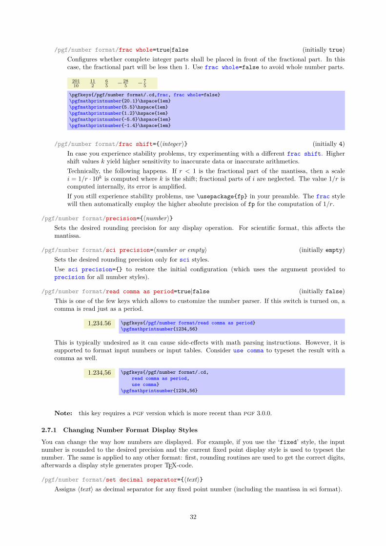
/pgf/number format/frac whole=true|false (initially true)Configures whether complete integer parts shall be placed in front of the fractional part. In thiscase, the fractional part will be less then 1. Use frac whole=false to avoid whole number parts.

20110

112

65 − 28

5 − 75

\pgfkeys{/pgf/number format/.cd,frac, frac whole=false}\pgfmathprintnumber{20.1}\hspace{1em}\pgfmathprintnumber{5.5}\hspace{1em}\pgfmathprintnumber{1.2}\hspace{1em}\pgfmathprintnumber{-5.6}\hspace{1em}\pgfmathprintnumber{-1.4}\hspace{1em}

/pgf/number format/frac shift={〈integer〉} (initially 4)In case you experience stability problems, try experimenting with a different frac shift. Highershift values k yield higher sensitivity to inaccurate data or inaccurate arithmetics.Technically, the following happens. If r < 1 is the fractional part of the mantissa, then a scalei = 1/r · 10k is computed where k is the shift; fractional parts of i are neglected. The value 1/r iscomputed internally, its error is amplified.If you still experience stability problems, use \usepackage{fp} in your preamble. The frac stylewill then automatically employ the higher absolute precision of fp for the computation of 1/r.

/pgf/number format/precision={〈number〉}Sets the desired rounding precision for any display operation. For scientific format, this affects themantissa.

/pgf/number format/sci precision=〈number or empty〉 (initially empty)Sets the desired rounding precision only for sci styles.Use sci precision={} to restore the initial configuration (which uses the argument provided toprecision for all number styles).

/pgf/number format/read comma as period=true|false (initially false)This is one of the few keys which allows to customize the number parser. If this switch is turned on, acomma is read just as a period.

1,234.56 \pgfkeys{/pgf/number format/read comma as period}\pgfmathprintnumber{1234,56}

This is typically undesired as it can cause side-effects with math parsing instructions. However, it issupported to format input numbers or input tables. Consider use comma to typeset the result with acomma as well.

1.234,56 \pgfkeys{/pgf/number format/.cd,read comma as period,use comma}

\pgfmathprintnumber{1234,56}

Note: this key requires a pgf version which is more recent than pgf 3.0.0.

2.7.1 Changing Number Format Display Styles

You can change the way how numbers are displayed. For example, if you use the ‘fixed’ style, the inputnumber is rounded to the desired precision and the current fixed point display style is used to typeset thenumber. The same is applied to any other format: first, rounding routines are used to get the correct digits,afterwards a display style generates proper TEX-code.

/pgf/number format/set decimal separator={〈text〉}Assigns 〈text〉 as decimal separator for any fixed point number (including the mantissa in sci format).

32

/pgf/number format/dec sep={〈text〉}Just another name for set decimal separator.

/pgf/number format/set thousands separator={〈text〉}Assigns 〈text〉 as thousands separator for any fixed point number (including the mantissa in sci format).

1234.56 \pgfkeys{/pgf/number format/.cd,fixed,fixed zerofill,precision=2,set thousands separator={}}

\pgfmathprintnumber{1234.56}

1234567890.00 \pgfkeys{/pgf/number format/.cd,fixed,fixed zerofill,precision=2,set thousands separator={}}

\pgfmathprintnumber{1234567890}

1.234.567.890.00 \pgfkeys{/pgf/number format/.cd,fixed,fixed zerofill,precision=2,set thousands separator={.}}


1, 234, 567, 890.00 \pgfkeys{/pgf/number format/.cd,fixed,fixed zerofill,precision=2,set thousands separator={,}}


1,234,567,890.00 \pgfkeys{/pgf/number format/.cd,fixed,fixed zerofill,precision=2,set thousands separator={{{{,}}}}}


The last example employs commas and disables the default comma-spacing.

/pgf/number format/1000 sep={〈text〉}Just another name for set thousands separator.

/pgf/number format/1000 sep in fractionals={〈boolean〉} (initially false)Configures whether the fractional part should also be grouped into groups of three digits.The value true will activate the 1000 sep for both integer and fractional parts. The value false willactivate 1000 sep only for the integer part.

1 234.123 456 7 \pgfkeys{/pgf/number format/.cd,fixed,precision=999,set thousands separator={\,},1000 sep in fractionals,

}\pgfmathprintnumber{1234.1234567}

1 234.123 456 700 \pgfkeys{/pgf/number format/.cd,fixed,fixed zerofill,precision=9,set thousands separator={\,},1000 sep in fractionals,

}\pgfmathprintnumber{1234.1234567}

33

/pgf/number format/min exponent for 1000 sep={〈number〉} (initially 0)Defines the smallest exponent in scientific notation which is required to draw thousand separators. Theexponent is the number of digits minus one, so 〈number〉 = 4 will use thousand separators starting with1e4 = 10000.

5 000; 1 000 000 \pgfkeys{/pgf/number format/.cd,int detect,1000 sep={\,},min exponent for 1000 sep=0}

\pgfmathprintnumber{5000}; \pgfmathprintnumber{1000000}

1000; 5000 \pgfkeys{/pgf/number format/.cd,int detect,1000 sep={\,},min exponent for 1000 sep=4}


10 000; 1 000 000 \pgfkeys{/pgf/number format/.cd,int detect,1000 sep={\,},min exponent for 1000 sep=4}


A value of 0 disables this feature (negative values are ignored).

/pgf/number format/use period (no value)A predefined style which installs periods ‘.’ as decimal separators and commas ‘,’ as thousands sepa-rators. This style is the default.

12.35 \pgfkeys{/pgf/number format/.cd,fixed,precision=2,use period}\pgfmathprintnumber{12.3456}

1,234.56 \pgfkeys{/pgf/number format/.cd,fixed,precision=2,use period}\pgfmathprintnumber{1234.56}

/pgf/number format/use comma (no value)A predefined style which installs commas ‘,’ as decimal separators and periods ‘.’ as thousands sepa-rators.

12,35 \pgfkeys{/pgf/number format/.cd,fixed,precision=2,use comma}\pgfmathprintnumber{12.3456}

1.234,56 \pgfkeys{/pgf/number format/.cd,fixed,precision=2,use comma}\pgfmathprintnumber{1234.56}

/pgf/number format/skip 0.={〈boolean〉} (initially false)Configures whether numbers like 0.1 shall be typeset as .1 or not.

.56 \pgfkeys{/pgf/number format/.cd,fixed,fixed zerofill,precision=2,skip 0.}


0.56 \pgfkeys{/pgf/number format/.cd,fixed,fixed zerofill,precision=2,skip 0.=false}


34

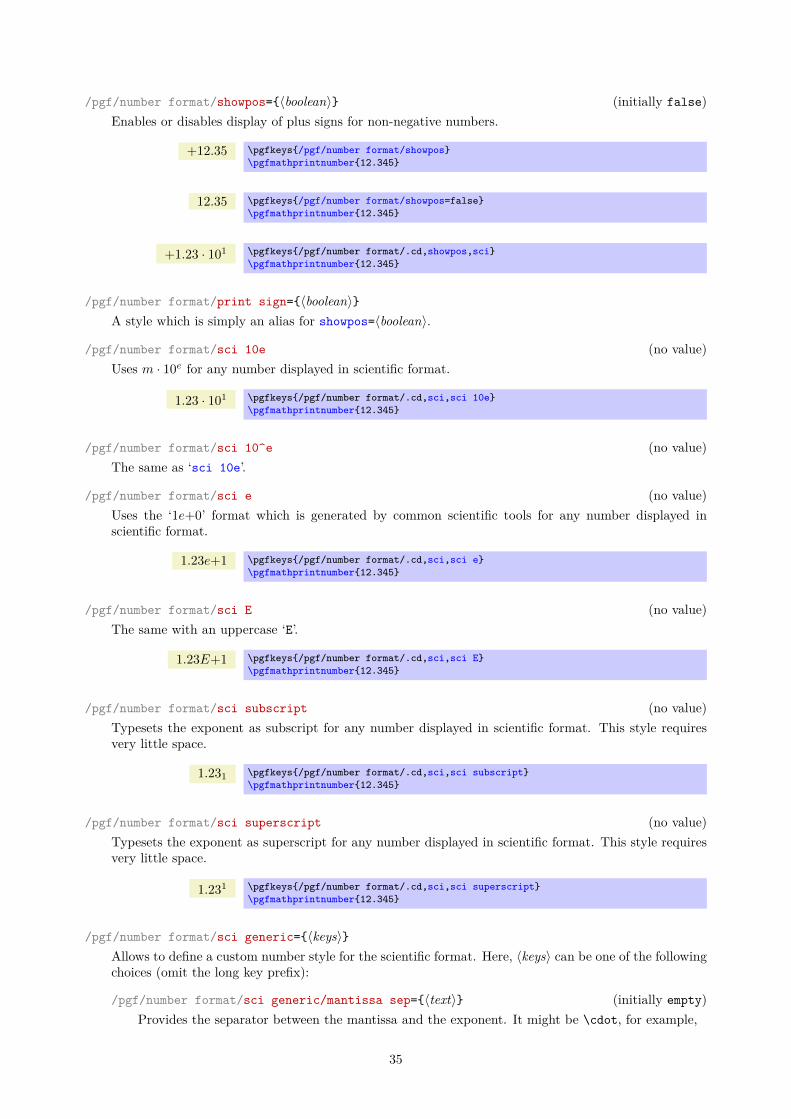
/pgf/number format/showpos={〈boolean〉} (initially false)Enables or disables display of plus signs for non-negative numbers.

+12.35 \pgfkeys{/pgf/number format/showpos}\pgfmathprintnumber{12.345}

12.35 \pgfkeys{/pgf/number format/showpos=false}\pgfmathprintnumber{12.345}

+1.23 · 101 \pgfkeys{/pgf/number format/.cd,showpos,sci}\pgfmathprintnumber{12.345}

/pgf/number format/print sign={〈boolean〉}A style which is simply an alias for showpos=〈boolean〉.

/pgf/number format/sci 10e (no value)Uses m · 10e for any number displayed in scientific format.

1.23 · 101 \pgfkeys{/pgf/number format/.cd,sci,sci 10e}\pgfmathprintnumber{12.345}

/pgf/number format/sci 10^e (no value)The same as ‘sci 10e’.

/pgf/number format/sci e (no value)Uses the ‘1e+0’ format which is generated by common scientific tools for any number displayed inscientific format.

1.23e+1 \pgfkeys{/pgf/number format/.cd,sci,sci e}\pgfmathprintnumber{12.345}

/pgf/number format/sci E (no value)The same with an uppercase ‘E’.

1.23E+1 \pgfkeys{/pgf/number format/.cd,sci,sci E}\pgfmathprintnumber{12.345}

/pgf/number format/sci subscript (no value)Typesets the exponent as subscript for any number displayed in scientific format. This style requiresvery little space.

1.231 \pgfkeys{/pgf/number format/.cd,sci,sci subscript}\pgfmathprintnumber{12.345}

/pgf/number format/sci superscript (no value)Typesets the exponent as superscript for any number displayed in scientific format. This style requiresvery little space.

1.231 \pgfkeys{/pgf/number format/.cd,sci,sci superscript}\pgfmathprintnumber{12.345}

/pgf/number format/sci generic={〈keys〉}Allows to define a custom number style for the scientific format. Here, 〈keys〉 can be one of the followingchoices (omit the long key prefix):

/pgf/number format/sci generic/mantissa sep={〈text〉} (initially empty)Provides the separator between the mantissa and the exponent. It might be \cdot, for example,

35

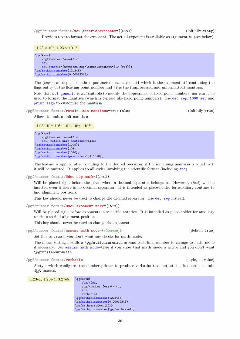
/pgf/number format/sci generic/exponent={〈text〉} (initially empty)Provides text to format the exponent. The actual exponent is available as argument #1 (see below).

1.23× 101; 1.23× 10−4

\pgfkeys{/pgf/number format/.cd,sci,sci generic={mantissa sep=\times,exponent={10^{#1}}}}

\pgfmathprintnumber{12.345};\pgfmathprintnumber{0.00012345}

The 〈keys〉 can depend on three parameters, namely on #1 which is the exponent, #2 containing theflags entity of the floating point number and #3 is the (unprocessed and unformatted) mantissa.Note that sci generic is not suitable to modify the appearance of fixed point numbers, nor can it beused to format the mantissa (which is typeset like fixed point numbers). Use dec sep, 1000 sep andprint sign to customize the mantissa.

/pgf/number format/retain unit mantissa=true|false (initially true)Allows to omit a unit mantissa.

1.05 · 101; 101; 1.01 · 103; −103;

\pgfkeys{/pgf/number format/.cd,sci, retain unit mantissa=false}

\pgfmathprintnumber{10.5};\pgfmathprintnumber{10};\pgfmathprintnumber{1010};\pgfmathprintnumber[precision=1]{-1010};

The feature is applied after rounding to the desired precision: if the remaining mantissa is equal to 1,it will be omitted. It applies to all styles involving the scientific format (including std).

/pgf/number format/@dec sep mark={〈text〉}Will be placed right before the place where a decimal separator belongs to. However, 〈text〉 will beinserted even if there is no decimal separator. It is intended as place-holder for auxiliary routines tofind alignment positions.This key should never be used to change the decimal separator! Use dec sep instead.

/pgf/number format/@sci exponent mark={〈text〉}Will be placed right before exponents in scientific notation. It is intended as place-holder for auxiliaryroutines to find alignment positions.This key should never be used to change the exponent!

/pgf/number format/assume math mode={〈boolean〉} (default true)Set this to true if you don’t want any checks for math mode.The initial setting installs a \pgfutilensuremath around each final number to change to math modeif necessary. Use assume math mode=true if you know that math mode is active and you don’t want\pgfutilensuremath.

/pgf/number format/verbatim (style, no value)A style which configures the number printer to produce verbatim text output, i.e. it doesn’t containTEX macros.

1.23e1; 1.23e-4; 3.27e6 \pgfkeys{/pgf/fpu,/pgf/number format/.cd,sci,verbatim}

\pgfmathprintnumber{12.345};\pgfmathprintnumber{0.00012345};\pgfmathparse{exp(15)}\pgfmathprintnumber{\pgfmathresult}

36

The style resets 1000 sep, dec sep, print sign, skip 0. and sets assume math mode. Furthermore,it installs a sci generic format for verbatim output of scientific numbers.However, it will still respect precision, fixed zerofill, sci zerofill and the overall styles fixed,sci, int detect (and their variants). It might be useful if you intend to write output files.

3 From Input Data To Output Tables: Data ProcessingThe conversion from an unprocessed input table to a final typesetted tabular code uses four stages for everycell,

1. Loading the table,

2. Preprocessing,

3. Typesetting,

4. Postprocessing.

The main idea is to select one typesetting algorithm (for example “format my numbers with the configurednumber style”). This algorithm usually doesn’t need to be changed. Fine-tuning can then be done usingzero, one or more preprocessors and postprocessors. Preprocessing can mean to select only particular rowsor to apply some sort of operation before the typesetting algorithm sees the content. Postprocessing meansto apply fine-tuning to the resulting TEX output – for example to deal with empty cells or to insert unitsuffixes or modify fonts for single cells.

Note that this kind of operation is processed column by column. As a consequence, the keys for prepro-cessing, typesetting, and postprocessing apply to styles on columns. They are unavailable for row styles likeevery last row. If you need to apply such content-based operations on specific rows, you have to writecode of sorts “if \pgfplotstablerow = generate content differently”.

3.1 Loading the tableThis first step to typeset a table involves the obvious input operations. Furthermore, the “new columncreation” operations explained in Section 4 are processed at this time. The table data is read (or acquired)as already explained earlier in this manual. Then, if columns are missing, column alias and create on usespecifications will be processed as part of the loading procedure. See Section 4 for details about columncreation.

3.2 Typesetting Cell ContentTypesetting cells means to take their value and “do something”. In many cases, this involves numberformatting routines. For example, the “raw” input data 12.56 might become 1.26 \cdot 10^1. Theresult of this stage is no longer useful for content-based computations. The typesetting step follows thepreprocessing step.

Typesetting cell content is applied in a column by column fashion, i.e. it can be configured for row styles.See the notes in the introduction of Section 3 for details how to apply such styles on specific rows only.

/pgfplots/table/assign cell content/.code={〈...〉}Allows to redefine the algorithm which assigns cell contents. The argument #1 is the (unformatted)contents of the input table.The resulting output needs to be written to /pgfplots/table/@cell content.

a b

data

1 23 45 67 8

\begin {tabular}{ccc}%\toprule &a&b\\\midrule %\multirow {4}{*}{data}&\pgfutilensuremath {1}&\pgfutilensuremath {2}\\%&\pgfutilensuremath {3}&\pgfutilensuremath {4}\\%&\pgfutilensuremath {5}&\pgfutilensuremath {6}\\%&\pgfutilensuremath {7}&\pgfutilensuremath {8}\\\bottomrule %\end {tabular}%

37

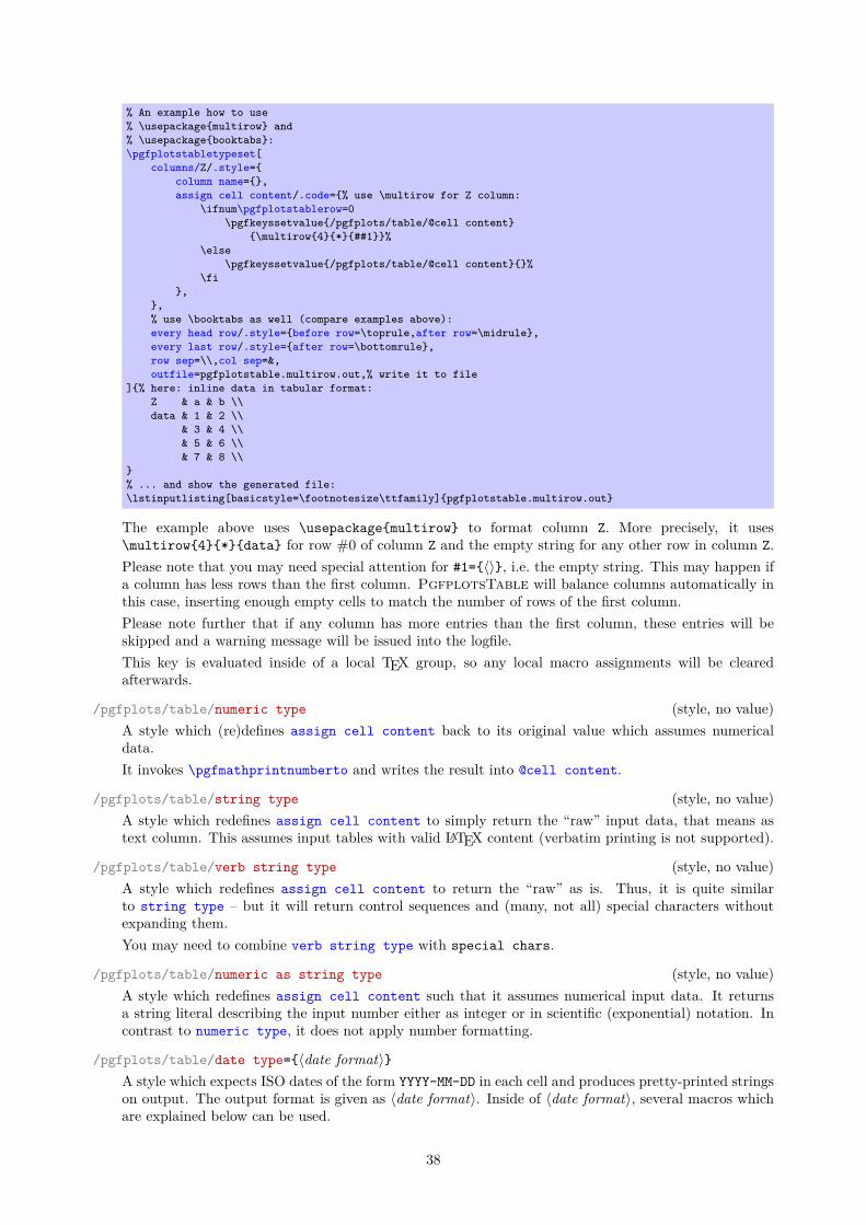
% An example how to use% \usepackage{multirow} and% \usepackage{booktabs}:\pgfplotstabletypeset[

columns/Z/.style={column name={},assign cell content/.code={% use \multirow for Z column:

\ifnum\pgfplotstablerow=0\pgfkeyssetvalue{/pgfplots/table/@cell content}

{\multirow{4}{*}{##1}}%\else

\pgfkeyssetvalue{/pgfplots/table/@cell content}{}%\fi

},},% use \booktabs as well (compare examples above):every head row/.style={before row=\toprule,after row=\midrule},every last row/.style={after row=\bottomrule},row sep=\\,col sep=&,outfile=pgfplotstable.multirow.out,% write it to file

]{% here: inline data in tabular format:Z & a & b \\data & 1 & 2 \\

& 3 & 4 \\& 5 & 6 \\& 7 & 8 \\

}% ... and show the generated file:\lstinputlisting[basicstyle=\footnotesize\ttfamily]{pgfplotstable.multirow.out}

The example above uses \usepackage{multirow} to format column Z. More precisely, it uses\multirow{4}{*}{data} for row #0 of column Z and the empty string for any other row in column Z.Please note that you may need special attention for #1={〈〉}, i.e. the empty string. This may happen ifa column has less rows than the first column. PgfplotsTable will balance columns automatically inthis case, inserting enough empty cells to match the number of rows of the first column.Please note further that if any column has more entries than the first column, these entries will beskipped and a warning message will be issued into the logfile.This key is evaluated inside of a local TEX group, so any local macro assignments will be clearedafterwards.

/pgfplots/table/numeric type (style, no value)A style which (re)defines assign cell content back to its original value which assumes numericaldata.It invokes \pgfmathprintnumberto and writes the result into @cell content.

/pgfplots/table/string type (style, no value)A style which redefines assign cell content to simply return the “raw” input data, that means astext column. This assumes input tables with valid LATEX content (verbatim printing is not supported).

/pgfplots/table/verb string type (style, no value)A style which redefines assign cell content to return the “raw” as is. Thus, it is quite similarto string type – but it will return control sequences and (many, not all) special characters withoutexpanding them.You may need to combine verb string type with special chars.

/pgfplots/table/numeric as string type (style, no value)A style which redefines assign cell content such that it assumes numerical input data. It returnsa string literal describing the input number either as integer or in scientific (exponential) notation. Incontrast to numeric type, it does not apply number formatting.

/pgfplots/table/date type={〈date format〉}A style which expects ISO dates of the form YYYY-MM-DD in each cell and produces pretty-printed stringson output. The output format is given as 〈date format〉. Inside of 〈date format〉, several macros whichare explained below can be used.

38

date account12008-01-03 602008-02-06 1202008-03-15 −102008-04-01 1,8002008-05-20 2,3002008-06-15 800

date account1January 2008 60February 2008 120March 2008 −10April 2008 1,800May 2008 2,300June 2008 800

% Requires% \usepackage{pgfcalendar}\pgfplotstableset{columns={date,account1}}

% plotdata/accounts.dat contains:%% date account1 account2 account3% 2008-01-03 60 1200 400% 2008-02-06 120 1600 410% 2008-03-15 -10 1600 410% 2008-04-01 1800 500 410% 2008-05-20 2300 500 410% 2008-06-15 800 1920 410

% Show the contents in `string type':\pgfplotstabletypeset[

columns/date/.style={string type}]{plotdata/accounts.dat}\hspace{1cm}% Show the contents in `date type':\pgfplotstabletypeset[

columns/date/.style={date type={\monthname\ \year}}]{plotdata/accounts.dat}

This style requires to load the pgf calendar package:

\usepackage{pgfcalendar}

\yearInside of 〈date format〉, this macro expands to the year as a number (like 2008).

\monthInside of 〈date format〉, this macro expands to the month as a number, starting with 1 (like 1).

\monthnameInside of 〈date format〉, this macro expands to the month’s name as set in the current language(like January). See below for how to change the language.

\monthshortnameInside of 〈date format〉, this macro expands to the month’s short name as set in the current language(like Jan). See below for how to change the language.

\dayInside of 〈date format〉, this macro expands to the day as number (like 31).

\weekdayInside of 〈date format〉, this macro expands to the weekday number (0 for Monday, 1 for Tuesdayetc.).

\weekdaynameInside of 〈date format〉, this macro expands to the weekday’s name in the current language (likeWednesday). See below for how to change the language.

\weekdayshortnameInside of 〈date format〉, this macro expands to the weekday’s short name in the current language(like Wed). See below for how to change the language.

39

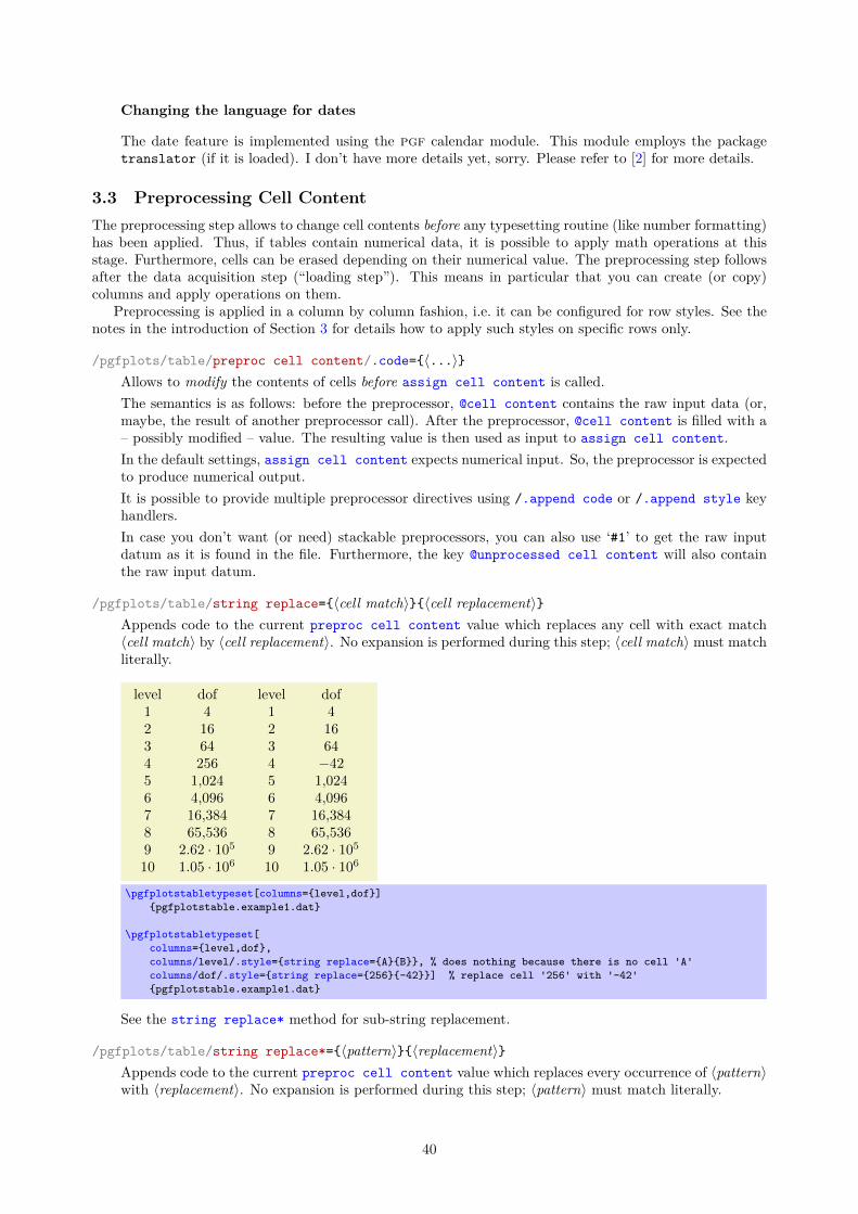
Changing the language for dates

The date feature is implemented using the pgf calendar module. This module employs the packagetranslator (if it is loaded). I don’t have more details yet, sorry. Please refer to [2] for more details.

3.3 Preprocessing Cell ContentThe preprocessing step allows to change cell contents before any typesetting routine (like number formatting)has been applied. Thus, if tables contain numerical data, it is possible to apply math operations at thisstage. Furthermore, cells can be erased depending on their numerical value. The preprocessing step followsafter the data acquisition step (“loading step”). This means in particular that you can create (or copy)columns and apply operations on them.

Preprocessing is applied in a column by column fashion, i.e. it can be configured for row styles. See thenotes in the introduction of Section 3 for details how to apply such styles on specific rows only.

/pgfplots/table/preproc cell content/.code={〈...〉}Allows to modify the contents of cells before assign cell content is called.The semantics is as follows: before the preprocessor, @cell content contains the raw input data (or,maybe, the result of another preprocessor call). After the preprocessor, @cell content is filled with a– possibly modified – value. The resulting value is then used as input to assign cell content.In the default settings, assign cell content expects numerical input. So, the preprocessor is expectedto produce numerical output.It is possible to provide multiple preprocessor directives using /.append code or /.append style keyhandlers.In case you don’t want (or need) stackable preprocessors, you can also use ‘#1’ to get the raw inputdatum as it is found in the file. Furthermore, the key @unprocessed cell content will also containthe raw input datum.

/pgfplots/table/string replace={〈cell match〉}{〈cell replacement〉}Appends code to the current preproc cell content value which replaces any cell with exact match〈cell match〉 by 〈cell replacement〉. No expansion is performed during this step; 〈cell match〉 must matchliterally.

level dof1 42 163 644 2565 1,0246 4,0967 16,3848 65,5369 2.62 · 10510 1.05 · 106

level dof1 42 163 644 −425 1,0246 4,0967 16,3848 65,5369 2.62 · 10510 1.05 · 106

\pgfplotstabletypeset[columns={level,dof}]{pgfplotstable.example1.dat}

\pgfplotstabletypeset[columns={level,dof},columns/level/.style={string replace={A}{B}}, % does nothing because there is no cell 'A'columns/dof/.style={string replace={256}{-42}}] % replace cell '256' with '-42'{pgfplotstable.example1.dat}

See the string replace* method for sub-string replacement.

/pgfplots/table/string replace*={〈pattern〉}{〈replacement〉}Appends code to the current preproc cell content value which replaces every occurrence of 〈pattern〉with 〈replacement〉. No expansion is performed during this step; 〈pattern〉 must match literally.

40


\pgfplotstabletypeset[string replace*={2}{6},col sep=&,row sep=\\]{

colA & colB & colC \\11 & 12 & 13 \\21 & 22 & 23 \\

}

/pgfplots/table/clear infinite (style, no value)Appends code to the current preproc cell content value which replaces every infinite number withthe empty string. This clears any cells with ±∞ and NaN.

/pgfplots/table/preproc/expr={〈math expression〉}Appends code to the current preproc cell content value which evaluates 〈math expression〉 for everycell. Arithmetics are carried out in floating point.Inside of 〈math expression〉, use one of the following expressions to get the current cell’s value.

• The string ‘##1’ expands to the cell’s content as it has been found in the input file, ignoringpreceding preprocessors.This is usually enough.

• The command \thisrow{〈the currently processed column name〉} expands to the current cell’scontent. This will also include the results of preceding preprocessors.Note that \thisrow{} in this context (inside of the preprocessor) is not as powerful as in thecontext of column creation routines: the argument must match exactly the name of the currentlyprocessed column name. You can also use the shorthand\thisrow{\pgfplotstablecolname}.

• The command \pgfkeysvalueof{/pgfplots/table/@cell content} is the same.

2 · level+ 4681012141618202224

\pgfplotstabletypeset[columns={level},columns/level/.style={

column name={$2\cdot \text{level}+4$},preproc/expr={2*##1 + 4}

}]


Empty cells won’t be processed, assuming that a math expression with an “empty number” will fail.Note that there is also an create col/expr which is more powerful than preproc/expr.

/pgfplots/table/multiply by={〈real number〉}Appends code to the current preproc cell content value which multiplies every cell by 〈real number〉.Arithmetics are carried out in floating point.

/pgfplots/table/divide by={〈real number〉}Appends code to the current preproc cell content value which divides every cell by 〈real number〉.Arithmetics are carried out in floating point.

/pgfplots/table/sqrt (style, no value)Appends code to the current preproc cell content value which takes the square root

√· of every

non-empty cell. Arithmetics are carried out in floating point.The following example copies the column error1 and applies sqrt to the copy.

41

ε√ε

2.500 · 10−1 5.000 · 10−1

6.250 · 10−2 2.500 · 10−1

1.563 · 10−2 1.250 · 10−1

3.906 · 10−3 6.250 · 10−2

9.766 · 10−4 3.125 · 10−2

2.441 · 10−4 1.562 · 10−2

6.104 · 10−5 7.813 · 10−3

1.526 · 10−5 3.906 · 10−3

3.815 · 10−6 1.953 · 10−3

9.537 · 10−7 9.766 · 10−4

\pgfplotstableset{columns={error1,sqrterror1},create on use/sqrterror1/.style={create col/copy=error1},columns/error1/.style={column name=$\epsilon$},columns/sqrterror1/.style={sqrt,column name=$\sqrt \epsilon$},sci,sci 10e,precision=3,sci zerofill

}\pgfplotstabletypeset{pgfplotstable.example1.dat}

Please take a look at Section 4 for details about create on use.

/pgfplots/table/multiply -1 (style, no value)Appends code to current preproc cell content value which multiplies every cell by −1. This styledoes the same job as multiply by=-1, it is just faster because only the sign changes.

dof error2 slopes24 7.58 · 10−1 −16 5.00 · 10−1 −0.364 2.87 · 10−1 −0.4256 1.44 · 10−1 −0.51,024 4.42 · 10−2 −0.854,096 1.70 · 10−2 −0.6916,384 8.20 · 10−3 −0.5265,536 3.91 · 10−3 −0.54

2.62 · 105 1.95 · 10−3 −0.51.05 · 106 9.77 · 10−4 −0.5

dof error2 slopes24 7.58 · 10−1 −16 5.00 · 10−1 0.364 2.87 · 10−1 0.4256 1.44 · 10−1 0.51,024 4.42 · 10−2 0.854,096 1.70 · 10−2 0.6916,384 8.20 · 10−3 0.5265,536 3.91 · 10−3 0.54

2.62 · 105 1.95 · 10−3 0.51.05 · 106 9.77 · 10−4 0.5

\pgfplotstableset{columns={dof,error2,slopes2},columns/error2/.style={sci,sci zerofill},columns/slopes2/.style={dec sep align,empty cells with={\ensuremath{-}}},create on use/slopes2/.style=

{create col/gradient loglog={dof}{error2}}}


\pgfplotstabletypeset[columns/slopes2/.append style={multiply -1}]{pgfplotstable.example1.dat}

/pgfplots/table/row predicate/.code={〈...〉}A boolean predicate which allows to select particular rows of the input table, based on the current row’sindex. The argument #1 contains the current row’s index (starting with 0, not counting comment linesor column names).The return value is assigned to the TEX-if \ifpgfplotstableuserow. If the boolean is not changed,the return value is true.

42

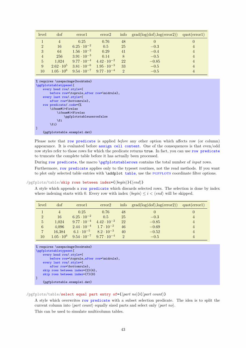
level dof error1 error2 info grad(log(dof),log(error2)) quot(error1)1 4 0.25 0.76 48 0 02 16 6.25 · 10−2 0.5 25 −0.3 43 64 1.56 · 10−2 0.29 41 −0.4 44 256 3.91 · 10−3 0.14 8 −0.5 45 1,024 9.77 · 10−4 4.42 · 10−2 22 −0.85 49 2.62 · 105 3.81 · 10−6 1.95 · 10−3 33 −0.5 410 1.05 · 106 9.54 · 10−7 9.77 · 10−4 2 −0.5 4




row predicate/.code={%\ifnum#1>4\relax

\ifnum#1<8\relax\pgfplotstableuserowfalse

\fi\fi}


Please note that row predicate is applied before any other option which affects row (or column)appearance. It is evaluated before assign cell content. One of the consequences is that even/oddrow styles refer to those rows for which the predicate returns true. In fact, you can use row predicateto truncate the complete table before it has actually been processed.During row predicate, the macro \pgfplotstablerows contains the total number of input rows.Furthermore, row predicate applies only to the typeset routines, not the read methods. If you wantto plot only selected table entries with \addplot table, use the pgfplots coordinate filter options.

/pgfplots/table/skip rows between index={〈begin〉}{〈end〉}A style which appends a row predicate which discards selected rows. The selection is done by indexwhere indexing starts with 0. Every row with index 〈begin〉 ≤ i < 〈end〉 will be skipped.

level dof error1 error2 info grad(log(dof),log(error2)) quot(error1)1 4 0.25 0.76 48 0 02 16 6.25 · 10−2 0.5 25 −0.3 45 1,024 9.77 · 10−4 4.42 · 10−2 22 −0.85 46 4,096 2.44 · 10−4 1.7 · 10−2 46 −0.69 47 16,384 6.1 · 10−5 8.2 · 10−3 40 −0.52 410 1.05 · 106 9.54 · 10−7 9.77 · 10−4 2 −0.5 4




skip rows between index={2}{4},skip rows between index={7}{9}


/pgfplots/table/select equal part entry of={〈part no〉}{〈part count〉}A style which overwrites row predicate with a subset selection predicate. The idea is to split thecurrent column into 〈part count〉 equally sized parts and select only 〈part no〉.This can be used to simulate multicolumn tables.

43

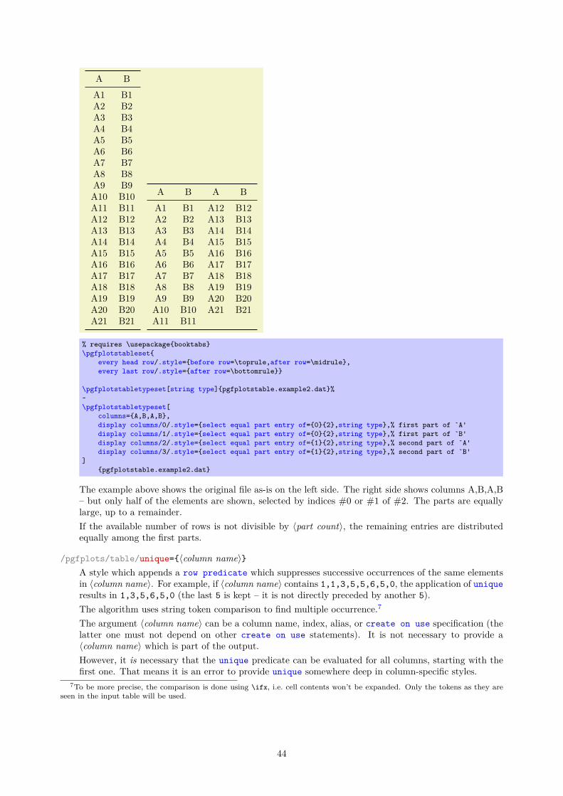
A BA1 B1A2 B2A3 B3A4 B4A5 B5A6 B6A7 B7A8 B8A9 B9A10 B10A11 B11A12 B12A13 B13A14 B14A15 B15A16 B16A17 B17A18 B18A19 B19A20 B20A21 B21

A B A BA1 B1 A12 B12A2 B2 A13 B13A3 B3 A14 B14A4 B4 A15 B15A5 B5 A16 B16A6 B6 A17 B17A7 B7 A18 B18A8 B8 A19 B19A9 B9 A20 B20A10 B10 A21 B21A11 B11

% requires \usepackage{booktabs}\pgfplotstableset{

every head row/.style={before row=\toprule,after row=\midrule},every last row/.style={after row=\bottomrule}}

\pgfplotstabletypeset[string type]{pgfplotstable.example2.dat}%~\pgfplotstabletypeset[

columns={A,B,A,B},display columns/0/.style={select equal part entry of={0}{2},string type},% first part of `A'display columns/1/.style={select equal part entry of={0}{2},string type},% first part of `B'display columns/2/.style={select equal part entry of={1}{2},string type},% second part of `A'display columns/3/.style={select equal part entry of={1}{2},string type},% second part of `B'


The example above shows the original file as-is on the left side. The right side shows columns A,B,A,B– but only half of the elements are shown, selected by indices #0 or #1 of #2. The parts are equallylarge, up to a remainder.If the available number of rows is not divisible by 〈part count〉, the remaining entries are distributedequally among the first parts.

/pgfplots/table/unique={〈column name〉}A style which appends a row predicate which suppresses successive occurrences of the same elementsin 〈column name〉. For example, if 〈column name〉 contains 1,1,3,5,5,6,5,0, the application of uniqueresults in 1,3,5,6,5,0 (the last 5 is kept – it is not directly preceded by another 5).The algorithm uses string token comparison to find multiple occurrence.7

The argument 〈column name〉 can be a column name, index, alias, or create on use specification (thelatter one must not depend on other create on use statements). It is not necessary to provide a〈column name〉 which is part of the output.However, it is necessary that the unique predicate can be evaluated for all columns, starting with thefirst one. That means it is an error to provide unique somewhere deep in column-specific styles.

7To be more precise, the comparison is done using \ifx, i.e. cell contents won’t be expanded. Only the tokens as they areseen in the input table will be used.

44

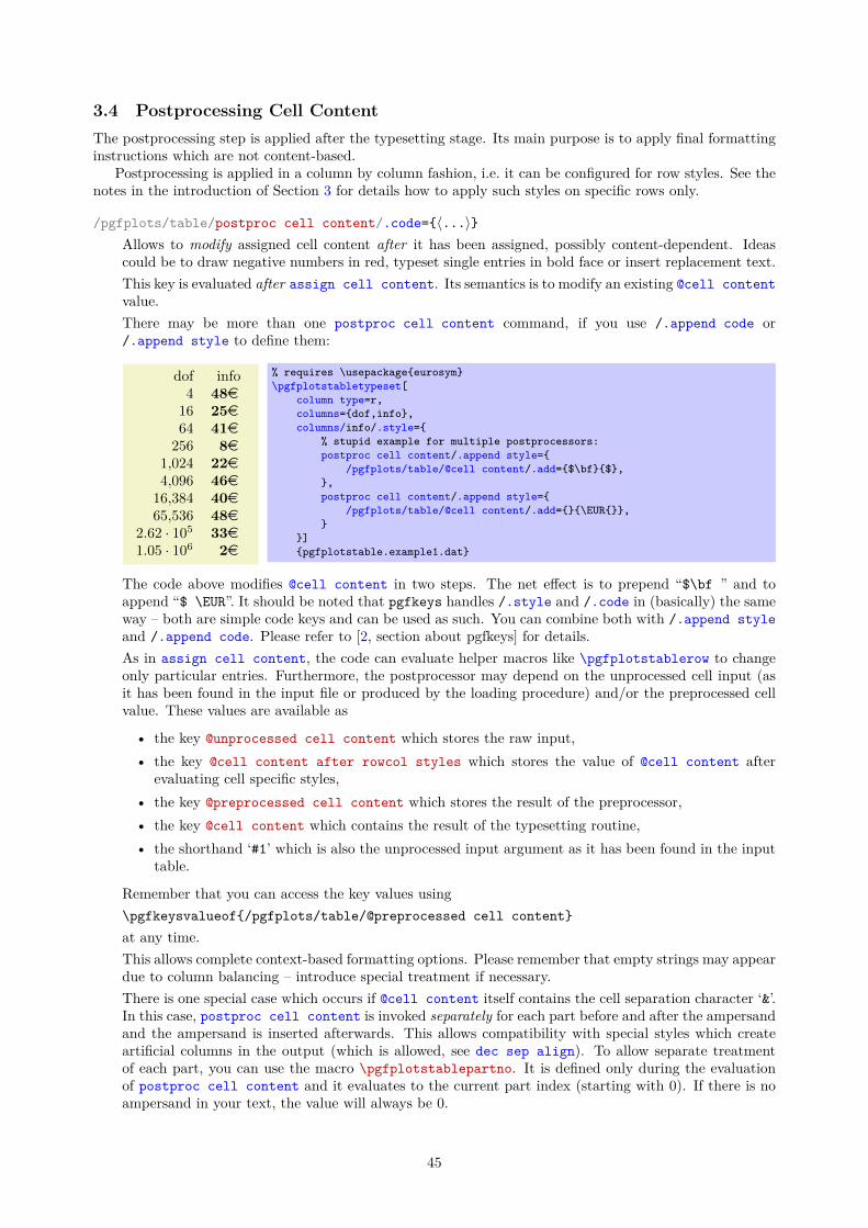
3.4 Postprocessing Cell ContentThe postprocessing step is applied after the typesetting stage. Its main purpose is to apply final formattinginstructions which are not content-based.

Postprocessing is applied in a column by column fashion, i.e. it can be configured for row styles. See thenotes in the introduction of Section 3 for details how to apply such styles on specific rows only.

/pgfplots/table/postproc cell content/.code={〈...〉}Allows to modify assigned cell content after it has been assigned, possibly content-dependent. Ideascould be to draw negative numbers in red, typeset single entries in bold face or insert replacement text.This key is evaluated after assign cell content. Its semantics is to modify an existing @cell contentvalue.There may be more than one postproc cell content command, if you use /.append code or/.append style to define them:

dof info4 48e16 25e64 41e256 8e

1,024 22e4,096 46e16,384 40e65,536 48e

2.62 · 105 33e1.05 · 106 2e

% requires \usepackage{eurosym}\pgfplotstabletypeset[

column type=r,columns={dof,info},columns/info/.style={

% stupid example for multiple postprocessors:postproc cell content/.append style={

/pgfplots/table/@cell content/.add={$\bf}{$},},postproc cell content/.append style={

/pgfplots/table/@cell content/.add={}{\EUR{}},}


The code above modifies @cell content in two steps. The net effect is to prepend “$\bf ” and toappend “$ \EUR”. It should be noted that pgfkeys handles /.style and /.code in (basically) the sameway – both are simple code keys and can be used as such. You can combine both with /.append styleand /.append code. Please refer to [2, section about pgfkeys] for details.As in assign cell content, the code can evaluate helper macros like \pgfplotstablerow to changeonly particular entries. Furthermore, the postprocessor may depend on the unprocessed cell input (asit has been found in the input file or produced by the loading procedure) and/or the preprocessed cellvalue. These values are available as

• the key @unprocessed cell content which stores the raw input,• the key @cell content after rowcol styles which stores the value of @cell content after

evaluating cell specific styles,• the key @preprocessed cell content which stores the result of the preprocessor,• the key @cell content which contains the result of the typesetting routine,• the shorthand ‘#1’ which is also the unprocessed input argument as it has been found in the input

table.

Remember that you can access the key values using\pgfkeysvalueof{/pgfplots/table/@preprocessed cell content}at any time.This allows complete context-based formatting options. Please remember that empty strings may appeardue to column balancing – introduce special treatment if necessary.There is one special case which occurs if @cell content itself contains the cell separation character ‘&’.In this case, postproc cell content is invoked separately for each part before and after the ampersandand the ampersand is inserted afterwards. This allows compatibility with special styles which createartificial columns in the output (which is allowed, see dec sep align). To allow separate treatmentof each part, you can use the macro \pgfplotstablepartno. It is defined only during the evaluationof postproc cell content and it evaluates to the current part index (starting with 0). If there is noampersand in your text, the value will always be 0.

45

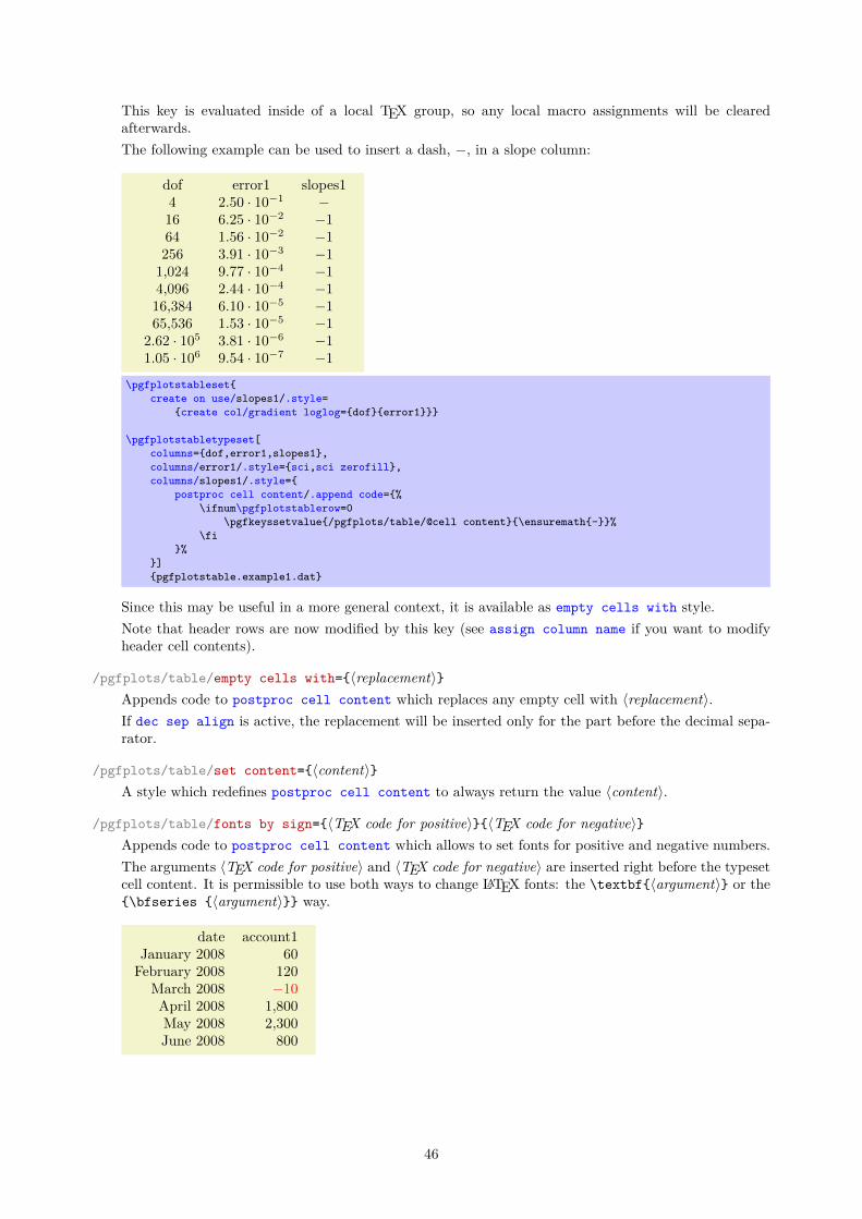
This key is evaluated inside of a local TEX group, so any local macro assignments will be clearedafterwards.The following example can be used to insert a dash, −, in a slope column:

dof error1 slopes14 2.50 · 10−1 −16 6.25 · 10−2 −164 1.56 · 10−2 −1256 3.91 · 10−3 −11,024 9.77 · 10−4 −14,096 2.44 · 10−4 −116,384 6.10 · 10−5 −165,536 1.53 · 10−5 −1

2.62 · 105 3.81 · 10−6 −11.05 · 106 9.54 · 10−7 −1

\pgfplotstableset{create on use/slopes1/.style=

{create col/gradient loglog={dof}{error1}}}

\pgfplotstabletypeset[columns={dof,error1,slopes1},columns/error1/.style={sci,sci zerofill},columns/slopes1/.style={

postproc cell content/.append code={%\ifnum\pgfplotstablerow=0

\pgfkeyssetvalue{/pgfplots/table/@cell content}{\ensuremath{-}}%\fi

}%}]{pgfplotstable.example1.dat}

Since this may be useful in a more general context, it is available as empty cells with style.Note that header rows are now modified by this key (see assign column name if you want to modifyheader cell contents).

/pgfplots/table/empty cells with={〈replacement〉}Appends code to postproc cell content which replaces any empty cell with 〈replacement〉.If dec sep align is active, the replacement will be inserted only for the part before the decimal sepa-rator.

/pgfplots/table/set content={〈content〉}A style which redefines postproc cell content to always return the value 〈content〉.

/pgfplots/table/fonts by sign={〈TEX code for positive〉}{〈TEX code for negative〉}Appends code to postproc cell content which allows to set fonts for positive and negative numbers.The arguments 〈TEX code for positive〉 and 〈TEX code for negative〉 are inserted right before the typesetcell content. It is permissible to use both ways to change LATEX fonts: the \textbf{〈argument〉} or the{\bfseries {〈argument〉}} way.

date account1January 2008 60February 2008 120

March 2008 −10April 2008 1,800May 2008 2,300June 2008 800

46

% Requires% \usepackage{pgfcalendar}

% plotdata/accounts.dat contains:%% date account1 account2 account3% 2008-01-03 60 1200 400% 2008-02-06 120 1600 410% 2008-03-15 -10 1600 410% 2008-04-01 1800 500 410% 2008-05-20 2300 500 410% 2008-06-15 800 1920 410

\pgfplotstabletypeset[columns={date,account1},column type=r,columns/date/.style={date type={\monthname\ \year}},columns/account1/.style={fonts by sign={}{\color{red}}}

]{plotdata/accounts.dat}

In fact, the arguments for this style don’t need to be font changes. The style fonts by sign insertsseveral braces and the matching argument into @cell content. To be more precise, it results in{〈TEX code for negative〉{〈cell value〉}} for negative numbers and{〈TEX code for positive〉{〈cell value〉}} for all other numbers.

4 Generating Data in New Tables or ColumnsIt is possible to create new tables from scratch or to change tables after they have been loaded from disk.

4.1 Creating New Tables From Scratch\pgfplotstablenew[〈options〉]{〈row count〉}{〈\table〉}\pgfplotstablenew*[〈options〉]{〈row count〉}{〈\table〉}

Creates a new table from scratch.The new table will contain all columns listed in the columns key. For \pgfplotstablenew, the columnskey needs to be provided in [〈options〉]. For \pgfplotstablenew*, the current value of columns isused, no matter where and when it has been set.Furthermore, there must be create on use statements (see the next subsection) for every column whichshall be generated.8 Columns are generated independently, in the order of appearance in columns. Assoon as a column is complete, it can be accessed using any of the basic level access mechanisms. Thus,you can build columns which depend on each other.The table will contain exactly 〈row count〉 rows. If 〈row count〉 is an \pgfplotstablegetrowsofstatement, that statement will be executed and the resulting number of rows be used. Otherwise, 〈rowcount〉 will be evaluated as number.

new45678910————

% this key setting could be provided in the document's preamble:\pgfplotstableset{

% define how the 'new' column shall be filled:create on use/new/.style={create col/set list={4,5,6,7,...,10}}}

% create a new table with 11 rows and column 'new':\pgfplotstablenew[columns={new}]{11}\loadedtable% show it:\pgfplotstabletypeset[empty cells with={---}]\loadedtable

8Currently, you need to provide at least one column: the implementation gets confused for completely empty tables. If youdo not provide any column name, a dummy column will be created.

47

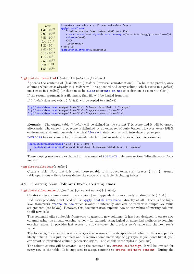
new1.31 · 10122.09 · 10133.56 · 10146.4 · 10151.22 · 10172.43 · 10185.11 · 10191.12 · 10212.59 · 10226.2 · 10231.55 · 1025

% create a new table with 11 rows and column 'new':\pgfplotstablenew[

% define how the 'new' column shall be filled:create on use/new/.style={create col/expr={factorial(15+\pgfplotstablerow)}},columns={new}]{11}\loadedtable

% show it:\pgfplotstabletypeset\loadedtable

\pgfplotstablevertcat{〈\table1〉}{〈\table2 or filename〉}Appends the contents of 〈\table2〉 to 〈\table1〉 (“vertical concatenation”). To be more precise, onlycolumns which exist already in 〈\table1〉 will be appended and every column which exists in 〈\table1〉must exist in 〈\table2〉 (or there must be alias or create on use specifications to generate them).If the second argument is a file name, that file will be loaded from disk.If 〈\table1〉 does not exist, 〈\table2〉 will be copied to 〈\table1〉.

\pgfplotstablevertcat{\output}{datafile1} % loads `datafile1' -> `\output'\pgfplotstablevertcat{\output}{datafile2} % appends rows of datafile2\pgfplotstablevertcat{\output}{datafile3} % appends rows of datafile3

Remark: The output table 〈\table1〉 will be defined in the current TEX scope and it will be erasedafterwards. The current TEX scope is delimited by an extra set of curly braces. However, every LATEXenvironment and, unfortunately, the TikZ \foreach statement as well, introduce TEX scopes.pgfplots has some some loop statements which do not introduce extra scopes. For example,

\pgfplotsforeachungrouped \i in {1,2,...,10} {%\pgfplotstablevertcat{\output}{datafile\i} % appends `datafile\i' -> `\output'

}%

These looping macros are explained in the manual of pgfplots, reference section “Miscellaneous Com-mands”

\pgfplotstableclear{〈\table〉}Clears a table. Note that it is much more reliable to introduce extra curly braces ‘{ ... }’ aroundtable operations – these braces define the scope of a variable (including tables).

4.2 Creating New Columns From Existing Ones\pgfplotstablecreatecol[〈options〉]{〈new col name〉}{〈\table〉}

Creates a new column named 〈new col name〉 and appends it to an already existing table 〈\table〉.End users probably don’t need to use \pgfplotstablecreatecol directly at all – there is the high-level framework create on use which invokes it internally and can be used with simple key–valueassignments (see below). However, this documentation explains how to use values of existing columnsto fill new cells.This command offers a flexible framework to generate new columns. It has been designed to create newcolumns using the already existing values – for example using logical or numerical methods to combineexisting values. It provides fast access to a row’s value, the previous row’s value and the next row’svalue.The following documentation is for everyone who wants to write specialized columns. It is not partic-ularly difficult; it is just technical and it requires some knowledge of pgfkeys. If you don’t like it, youcan resort to predefined column generation styles – and enable those styles in 〈options〉.The column entries will be created using the command key create col/assign. It will be invoked forevery row of the table. It is supposed to assign contents to create col/next content. During the

48

evaluation, the macro \thisrow{〈col name〉} expands to the current row’s value of the column identifiedby 〈col name〉. Furthermore, \nextrow{〈col name〉} expands to the next row’s value of the designatedcolumn and \prevrow{〈col name〉} expands to the value of the previous row.So, the idea is to simply redefine the command key create col/assign in such a way that it fills newcells as desired.Two special assign routines are available for the first and last row: The contents for the last rowis computed with create col/assign last. Its semantics is the same. The contents for the firstrow is computed with create col/assign first to simplify special cases here. These first and lastcommands are optional, their default is to invoke the normal assign routine.The evaluation of the assign keys is done in local TEX groups (i.e. any local definitions will be clearedafterwards).The following macros are useful during cell assignments:

1. \prevrow{〈col name〉} / \getprevrow{〈col name〉}{〈\macro〉}These two routines return the value stored in the previous row of the designated column 〈col name〉.The get routine stores it into 〈\macro〉.The argument 〈col name〉 has to denote either an existing column name or one for which analias/〈col name〉 exists.

2. \thisrow{〈col name〉} / \getthisrow{〈col name〉}{〈\macro〉}These two routines return the current row’s value stored in the designated column. The get routinestores it into 〈\macro〉.The argument 〈col name〉 has to denote either an existing column name or one for which analias/〈col name〉 exists.

3. \nextrow{〈col name〉} / \getnextrow{〈col name〉}{〈\macro〉}These two routines return the next row’s value.The argument 〈col name〉 has to denote either an existing column name or one for which analias/〈col name〉 exists.

4. \pgfplotstablerow and \pgfplotstablerows which contain the current row’s index and the totalnumber of rows, respectively. See page 16 for details.

5. \pgfmathaccuma and \pgfmathaccumb can be used to transport intermediate results. Both main-tain their value from one column assignment to the next. All other local variables will be deletedafter leaving the assignment routines. The initial value is the empty string for both of them unlessthey are already initialized by column creation styles.

6. \pgfplotstablename a macro containing the name of the currently processed table (i.e. it containsthe second argument of \pgfplotstablecreatecol).

7. commands which are valid throughout every part of this package, for example \pgfplotstablerowto get the current row index or \pgfplotstablerows to get the total number of rows.

The 〈col name〉 is expected to be a physical column name, no alias or column index is allowed (unlesscolumn indices and column names are the same).The following example takes our well-known input table and creates a copy of the level column.Furthermore, it produces a lot of output to show the available macros. Finally, it uses \pgfkeyslet toassign the contents of the resulting \entry to next content.

level new1 thisrow=1; nextrow=2. (#0/10)2 thisrow=2; nextrow=3. (#1/10)3 thisrow=3; nextrow=4. (#2/10)4 thisrow=4; nextrow=5. (#3/10)5 thisrow=5; nextrow=6. (#4/10)6 thisrow=6; nextrow=7. (#5/10)7 thisrow=7; nextrow=8. (#6/10)8 thisrow=8; nextrow=9. (#7/10)9 thisrow=9; nextrow=10. (#8/10)10 thisrow=10; nextrow=. (#9/10)

49

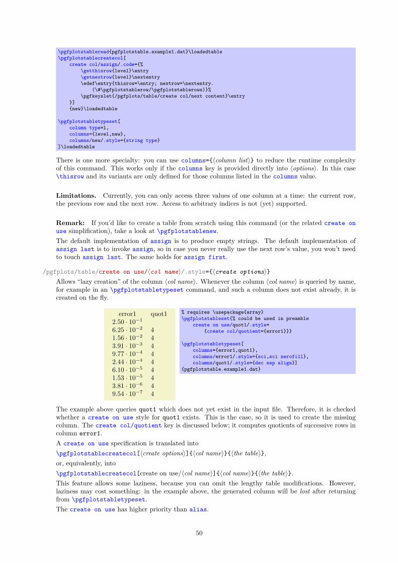
\pgfplotstableread{pgfplotstable.example1.dat}\loadedtable\pgfplotstablecreatecol[

create col/assign/.code={%\getthisrow{level}\entry\getnextrow{level}\nextentry\edef\entry{thisrow=\entry; nextrow=\nextentry.

(\#\pgfplotstablerow/\pgfplotstablerows)}%\pgfkeyslet{/pgfplots/table/create col/next content}\entry

}]{new}\loadedtable

\pgfplotstabletypeset[column type=l,columns={level,new},columns/new/.style={string type}

]\loadedtable

There is one more specialty: you can use columns={〈column list〉} to reduce the runtime complexityof this command. This works only if the columns key is provided directly into 〈options〉. In this case\thisrow and its variants are only defined for those columns listed in the columns value.

Limitations. Currently, you can only access three values of one column at a time: the current row,the previous row and the next row. Access to arbitrary indices is not (yet) supported.

Remark: If you’d like to create a table from scratch using this command (or the related create onuse simplification), take a look at \pgfplotstablenew.The default implementation of assign is to produce empty strings. The default implementation ofassign last is to invoke assign, so in case you never really use the next row’s value, you won’t needto touch assign last. The same holds for assign first.

/pgfplots/table/create on use/〈col name〉/.style={〈create options〉}Allows “lazy creation” of the column 〈col name〉. Whenever the column 〈col name〉 is queried by name,for example in an \pgfplotstabletypeset command, and such a column does not exist already, it iscreated on the fly.

error1 quot12.50 · 10−1

6.25 · 10−2 41.56 · 10−2 43.91 · 10−3 49.77 · 10−4 42.44 · 10−4 46.10 · 10−5 41.53 · 10−5 43.81 · 10−6 49.54 · 10−7 4

% requires \usepackage{array}\pgfplotstableset{% could be used in preamble

create on use/quot1/.style={create col/quotient={error1}}}

\pgfplotstabletypeset[columns={error1,quot1},columns/error1/.style={sci,sci zerofill},columns/quot1/.style={dec sep align}]


The example above queries quot1 which does not yet exist in the input file. Therefore, it is checkedwhether a create on use style for quot1 exists. This is the case, so it is used to create the missingcolumn. The create col/quotient key is discussed below; it computes quotients of successive rows incolumn error1.A create on use specification is translated into\pgfplotstablecreatecol[〈create options〉]{〈col name〉}{〈the table〉},or, equivalently, into\pgfplotstablecreatecol[create on use/〈col name〉]{〈col name〉}{〈the table〉}.This feature allows some laziness, because you can omit the lengthy table modifications. However,laziness may cost something: in the example above, the generated column will be lost after returningfrom \pgfplotstabletypeset.The create on use has higher priority than alias.

50

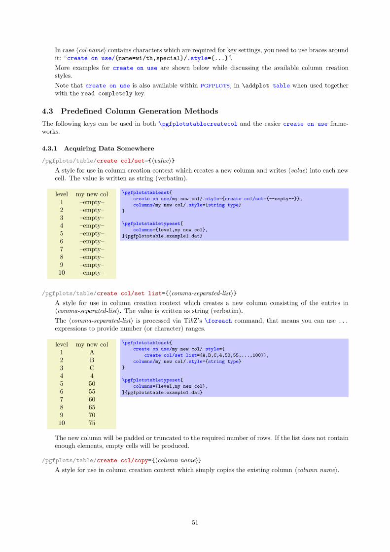
In case 〈col name〉 contains characters which are required for key settings, you need to use braces aroundit: “create on use/{name=wi/th,special}/.style={...}”.More examples for create on use are shown below while discussing the available column creationstyles.Note that create on use is also available within pgfplots, in \addplot table when used togetherwith the read completely key.

4.3 Predefined Column Generation MethodsThe following keys can be used in both \pgfplotstablecreatecol and the easier create on use frame-works.

4.3.1 Acquiring Data Somewhere

/pgfplots/table/create col/set={〈value〉}A style for use in column creation context which creates a new column and writes 〈value〉 into each newcell. The value is written as string (verbatim).

level my new col1 –empty–2 –empty–3 –empty–4 –empty–5 –empty–6 –empty–7 –empty–8 –empty–9 –empty–10 –empty–

\pgfplotstableset{create on use/my new col/.style={create col/set={--empty--}},columns/my new col/.style={string type}

}

\pgfplotstabletypeset[columns={level,my new col},


/pgfplots/table/create col/set list={〈comma-separated-list〉}A style for use in column creation context which creates a new column consisting of the entries in〈comma-separated-list〉. The value is written as string (verbatim).The 〈comma-separated-list〉 is processed via TikZ’s \foreach command, that means you can use ...expressions to provide number (or character) ranges.

level my new col1 A2 B3 C4 45 506 557 608 659 7010 75

\pgfplotstableset{create on use/my new col/.style={

create col/set list={A,B,C,4,50,55,...,100}},columns/my new col/.style={string type}

}

\pgfplotstabletypeset[columns={level,my new col},


The new column will be padded or truncated to the required number of rows. If the list does not containenough elements, empty cells will be produced.

/pgfplots/table/create col/copy={〈column name〉}A style for use in column creation context which simply copies the existing column 〈column name〉.

51

level Copy of level1 12 23 34 45 56 67 78 89 910 10

\pgfplotstableset{create on use/new/.style={create col/copy={level}}

}

\pgfplotstabletypeset[columns={level,new},columns/new/.style={column name=Copy of level}


/pgfplots/table/create col/copy column from table={〈file name or \macro〉}{〈column name〉}A style for use in column creation context which creates a new column consisting of the entries in〈column name〉 of the provided table. The argument may be either a file name or an already loadedtable (i.e. a 〈\macro〉 as returned by \pgfplotstableread).You can use this style, possibly combined with \pgfplotstablenew, to merge one common sort ofcolumn from different tables into one large table.The cell values are written as string (verbatim).The new column will be padded or truncated to the required number of rows. If the list does not containenough elements, empty cells will be produced.

4.3.2 Mathematical Operations

/pgf/fpu=true|false (initially true)Before we start to describe the column generation methods, one word about the math library. The coreis always the pgf math engine written by Mark Wibrow and Till Tantau. However, this engine hasbeen written to produce graphics and is not suitable for scientific computing.I added a high-precision floating point library to pgf which will be part of releases newer than pgf2.00. It offers the full range of IEEE double precision computing in TEX. This FPU is also part of Pgf-plotsTable, and it is activated by default for create col/expr and all other predefined mathematicalmethods.The FPU won’t be active for newly defined numerical styles (although it is active for the predefinedmathematical expression parsing styles like create col/expr). If you want to add own routines orstyles, you will need to use

\pgfkeys{/pgf/fpu=true}

in order to activate the extended precision. The standard math parser is limited to fixed point numbersin the range of ±16384.00000.

/pgfplots/table/create col/expr={〈math expression〉}A style for use in \pgfplotstablecreatecol which uses 〈math expression〉 to assign contents for thenew column.

level 2·level1 22 43 64 85 106 127 148 169 1810 20

\pgfplotstableset{create on use/new/.style={

create col/expr={\thisrow{level}*2}}}

\pgfplotstabletypeset[columns={level,new},columns/new/.style={column name=$2\cdot $level}


52

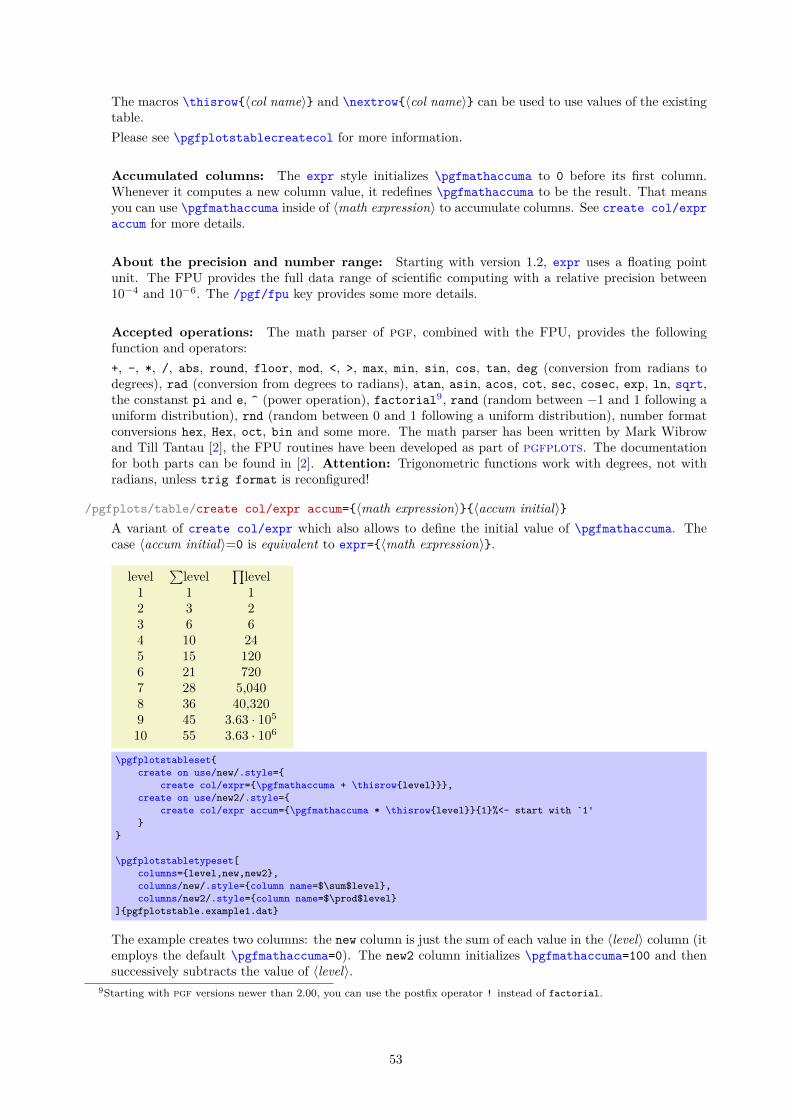
The macros \thisrow{〈col name〉} and \nextrow{〈col name〉} can be used to use values of the existingtable.Please see \pgfplotstablecreatecol for more information.

Accumulated columns: The expr style initializes \pgfmathaccuma to 0 before its first column.Whenever it computes a new column value, it redefines \pgfmathaccuma to be the result. That meansyou can use \pgfmathaccuma inside of 〈math expression〉 to accumulate columns. See create col/expraccum for more details.

About the precision and number range: Starting with version 1.2, expr uses a floating pointunit. The FPU provides the full data range of scientific computing with a relative precision between10−4 and 10−6. The /pgf/fpu key provides some more details.

Accepted operations: The math parser of pgf, combined with the FPU, provides the followingfunction and operators:+, -, *, /, abs, round, floor, mod, <, >, max, min, sin, cos, tan, deg (conversion from radians todegrees), rad (conversion from degrees to radians), atan, asin, acos, cot, sec, cosec, exp, ln, sqrt,the constanst pi and e, ^ (power operation), factorial9, rand (random between −1 and 1 following auniform distribution), rnd (random between 0 and 1 following a uniform distribution), number formatconversions hex, Hex, oct, bin and some more. The math parser has been written by Mark Wibrowand Till Tantau [2], the FPU routines have been developed as part of pgfplots. The documentationfor both parts can be found in [2]. Attention: Trigonometric functions work with degrees, not withradians, unless trig format is reconfigured!

/pgfplots/table/create col/expr accum={〈math expression〉}{〈accum initial〉}A variant of create col/expr which also allows to define the initial value of \pgfmathaccuma. Thecase 〈accum initial〉=0 is equivalent to expr={〈math expression〉}.

level∑

level∏level

1 1 12 3 23 6 64 10 245 15 1206 21 7207 28 5,0408 36 40,3209 45 3.63 · 10510 55 3.63 · 106

\pgfplotstableset{create on use/new/.style={

create col/expr={\pgfmathaccuma + \thisrow{level}}},create on use/new2/.style={

create col/expr accum={\pgfmathaccuma * \thisrow{level}}{1}%<- start with `1'}

}

\pgfplotstabletypeset[columns={level,new,new2},columns/new/.style={column name=$\sum$level},columns/new2/.style={column name=$\prod$level}


The example creates two columns: the new column is just the sum of each value in the 〈level〉 column (itemploys the default \pgfmathaccuma=0). The new2 column initializes \pgfmathaccuma=100 and thensuccessively subtracts the value of 〈level〉.

9Starting with pgf versions newer than 2.00, you can use the postfix operator ! instead of factorial.

53

/pgfplots/table/create col/quotient={〈column name〉}A style for use in \pgfplotstablecreatecol which computes the quotient ci := mi−1/mi for everyentry i = 1, . . . , (n− 1) in the column identified with 〈column name〉. The first value c0 is kept empty.

error1 error2 quot1 quot22.50 · 10−1 7.58 · 10−1

6.25 · 10−2 5.00 · 10−1 4 1.521.56 · 10−2 2.87 · 10−1 4 1.743.91 · 10−3 1.44 · 10−1 4 29.77 · 10−4 4.42 · 10−2 4 3.252.44 · 10−4 1.70 · 10−2 4 2.66.10 · 10−5 8.20 · 10−3 4 2.071.53 · 10−5 3.91 · 10−3 4 2.13.81 · 10−6 1.95 · 10−3 4 29.54 · 10−7 9.77 · 10−4 4 2

% requires \usepackage{array}\pgfplotstableset{% configuration, for example, in preamble:

create on use/quot1/.style={create col/quotient=error1},create on use/quot2/.style={create col/quotient=error2},columns={error1,error2,quot1,quot2},%% display styles:columns/error1/.style={sci,sci zerofill},columns/error2/.style={sci,sci zerofill},columns/quot1/.style={dec sep align},columns/quot2/.style={dec sep align}

}


This style employs methods of the floating point unit, that means it works with a relative precision ofabout 10−7 (7 significant digits in the mantissa).

/pgfplots/table/create col/iquotient={〈column name〉}Like create col/quotient, but the quotient is inverse.

/pgfplots/table/create col/dyadic refinement rate={〈column name〉}A style for use in \pgfplotstablecreatecol which computes the convergence rate α of the data incolumn 〈column name〉. The contents of 〈column name〉 is assumed to be something like ei(hi) = O(hα

i ).Assuming a dyadic refinement relation from one row to the next, hi = hi−1/2, we have hα

i−1/(hi−1/2)α =

2α, so we get α using

ci := log2

(ei−1

ei

).

The first value c0 is kept empty.

error1 error2 rate1 rate22.50 · 10−1 7.58 · 10−1

6.25 · 10−2 5.00 · 10−1 2 0.61.56 · 10−2 2.87 · 10−1 2 0.83.91 · 10−3 1.44 · 10−1 2 19.77 · 10−4 4.42 · 10−2 2 1.72.44 · 10−4 1.70 · 10−2 2 1.386.10 · 10−5 8.20 · 10−3 2 1.051.53 · 10−5 3.91 · 10−3 2 1.073.81 · 10−6 1.95 · 10−3 2 19.54 · 10−7 9.77 · 10−4 2 1

54

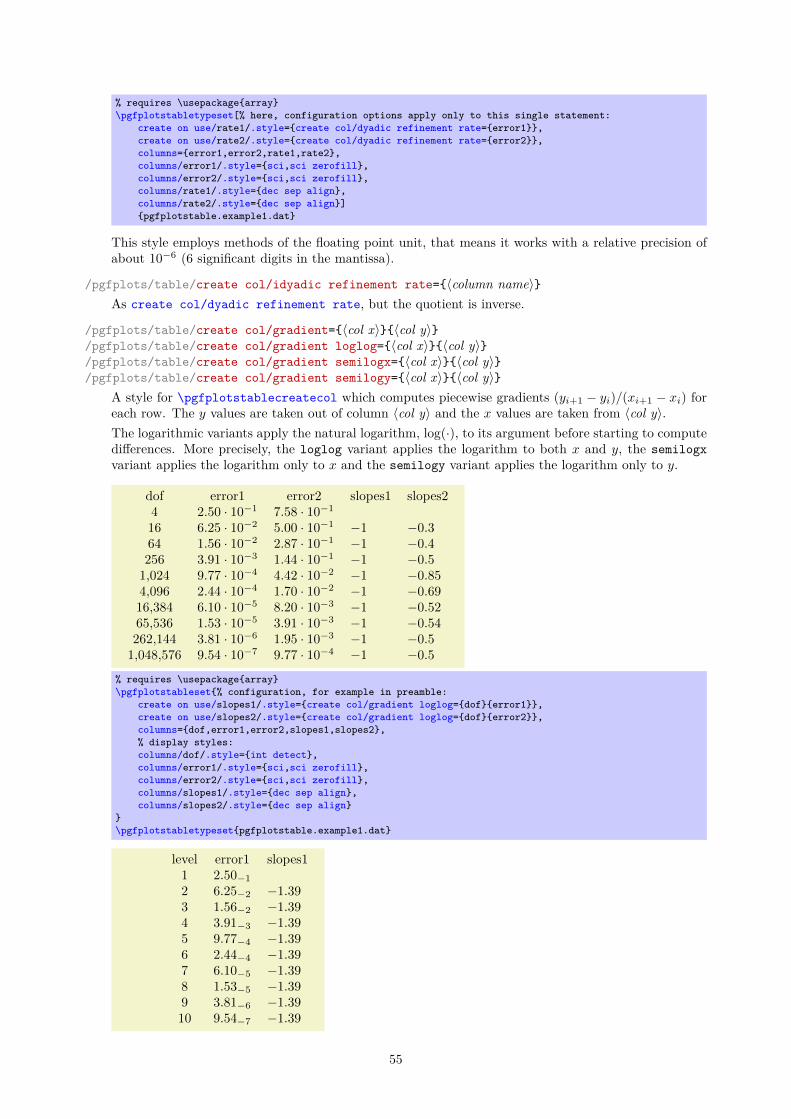
% requires \usepackage{array}\pgfplotstabletypeset[% here, configuration options apply only to this single statement:

create on use/rate1/.style={create col/dyadic refinement rate={error1}},create on use/rate2/.style={create col/dyadic refinement rate={error2}},columns={error1,error2,rate1,rate2},columns/error1/.style={sci,sci zerofill},columns/error2/.style={sci,sci zerofill},columns/rate1/.style={dec sep align},columns/rate2/.style={dec sep align}]{pgfplotstable.example1.dat}


/pgfplots/table/create col/idyadic refinement rate={〈column name〉}As create col/dyadic refinement rate, but the quotient is inverse.

/pgfplots/table/create col/gradient={〈col x〉}{〈col y〉}/pgfplots/table/create col/gradient loglog={〈col x〉}{〈col y〉}/pgfplots/table/create col/gradient semilogx={〈col x〉}{〈col y〉}/pgfplots/table/create col/gradient semilogy={〈col x〉}{〈col y〉}

A style for \pgfplotstablecreatecol which computes piecewise gradients (yi+1 − yi)/(xi+1 − xi) foreach row. The y values are taken out of column 〈col y〉 and the x values are taken from 〈col y〉.The logarithmic variants apply the natural logarithm, log(·), to its argument before starting to computedifferences. More precisely, the loglog variant applies the logarithm to both x and y, the semilogxvariant applies the logarithm only to x and the semilogy variant applies the logarithm only to y.

dof error1 error2 slopes1 slopes24 2.50 · 10−1 7.58 · 10−1

16 6.25 · 10−2 5.00 · 10−1 −1 −0.364 1.56 · 10−2 2.87 · 10−1 −1 −0.4256 3.91 · 10−3 1.44 · 10−1 −1 −0.51,024 9.77 · 10−4 4.42 · 10−2 −1 −0.854,096 2.44 · 10−4 1.70 · 10−2 −1 −0.6916,384 6.10 · 10−5 8.20 · 10−3 −1 −0.5265,536 1.53 · 10−5 3.91 · 10−3 −1 −0.54262,144 3.81 · 10−6 1.95 · 10−3 −1 −0.51,048,576 9.54 · 10−7 9.77 · 10−4 −1 −0.5

% requires \usepackage{array}\pgfplotstableset{% configuration, for example in preamble:

create on use/slopes1/.style={create col/gradient loglog={dof}{error1}},create on use/slopes2/.style={create col/gradient loglog={dof}{error2}},columns={dof,error1,error2,slopes1,slopes2},% display styles:columns/dof/.style={int detect},columns/error1/.style={sci,sci zerofill},columns/error2/.style={sci,sci zerofill},columns/slopes1/.style={dec sep align},columns/slopes2/.style={dec sep align}


level error1 slopes11 2.50−1

2 6.25−2 −1.393 1.56−2 −1.394 3.91−3 −1.395 9.77−4 −1.396 2.44−4 −1.397 6.10−5 −1.398 1.53−5 −1.399 3.81−6 −1.3910 9.54−7 −1.39

55

% requires \usepackage{array}\pgfplotstableset{% configuration, for example in preamble:

create on use/slopes1/.style={create col/gradient semilogy={level}{error1}},columns={level,error1,slopes1},% display styles:columns/level/.style={int detect},columns/error1/.style={sci,sci zerofill,sci subscript},columns/slopes1/.style={dec sep align}



/pgfplots/table/create col/linear regression={〈key-value-config〉}Computes a linear (least squares) regression y(x) = a · x+ b using the sample data (xi, yi) which has tobe specified inside of 〈key-value-config〉.

x y regression1 1 −2.332 4 4.673 9 11.674 16 18.675 25 25.676 36 32.67

The slope is ‘7.0e0’.

% load table from somewhere:\pgfplotstableread{

x y1 12 43 94 165 256 36

}\loadedtbl

% create the `regression' column:\pgfplotstablecreatecol[linear regression]

{regression}{\loadedtbl}

% store slope\xdef\slope{\pgfplotstableregressiona}

\pgfplotstabletypeset\loadedtbl\\

The slope is `\slope'.

The example above loads a table from inline data, appends a column named ‘regression’ and typesetsit. Since no 〈key-value-config〉 has been provided, x=[index]0 and y=[index]1 will be used. The\xdef\slope{...} command stores the ‘a’ value of the regression line into a newly defined macro‘\slope’.10

The complete documentation for this feature has been moved to pgfplots due to its close relation toplotting. Please refer to the pgfplots manual coming with this package.

/pgfplots/table/create col/function graph cut y={〈cut value〉}{〈common options〉}{〈one key–valueset for each plot〉}A specialized style for use in create on use statements which computes cuts of (one or more) discreteplots y(x1), . . . , y(xN ) with a fixed 〈cut value〉. The xi are written into the table’s cells.In a cost–accuracy plot, this feature allows to extract the cost for fixed accuracy. The dual feature withcut x allows to compute the accuracy for fixed cost.

10The \xdef means “global expanded definition”: it expands the argument until it can’t be expanded any further and assignsa (global) name to the result. See any TEX book for details.

56

cut53.66601.83

101 102 103 104

10−7

10−5

10−3

10−1

x = 53.66

x = 601.83

% Preamble: \pgfplotsset{width=7cm,compat=1.18}

\pgfplotstablenew[create on use/cut/.style={create col/function graph cut y=

{2.5e-4} % search for fixed L2 = 2.5e-4{x=Basis,y=L2,ymode=log,xmode=log} % double log, each function is L2(Basis)% now, provide each single function f_i(Basis):{{table=plotdata/newexperiment1.dat},{table=plotdata/newexperiment2.dat}}

},columns={cut}]{2}\loadedtable

% Show the data:\pgfplotstabletypeset{\loadedtable}

\begin{tikzpicture}\begin{loglogaxis}

\addplot table[x=Basis,y=L2] {plotdata/newexperiment1.dat};\addplot table[x=Basis,y=L2] {plotdata/newexperiment2.dat};\draw[blue!30!white] (1,2.5e-4) -- (1e5,2.5e-4);\node[pin=-90:{$x=53.66$}] at (53.66,2.5e-4) {};\node[pin=45:{$x=601.83$}] at (601.83,2.5e-4) {};

\end{loglogaxis}\end{tikzpicture}

In the example above, we are searching for x1 and x2 such that f1(x1) = 2.5·10−4 and f2(x2) = 2.5·10−4.On the left is the automatically computed result. On the right is a problem illustration with properannotation using pgfplots to visualize the results. The 〈cut value〉 is set to 2.5e-4. The 〈commonoptions〉 contain the problem setup; in our case logarithmic scales and column names. The thirdargument is a comma-separated-list. Each element i is a set of keys describing how to get fi(·).During both 〈common options〉 and 〈one key–value set for each plot〉, the following keys can be used:

• table={〈table file or \macro〉}: either a file name or an already loaded table where to get the datapoints,

• x={〈col name〉}: the column name of the x-axis,• y={〈col name〉}: the column name of the y-axis.• foreach={〈\foreach loop head〉}{〈file name pattern〉} This somewhat advanced syntax allows to

collect tables in a loop automatically:

cut53.66601.83

57

\pgfplotstablenew[% same as above...create on use/cut/.style={create col/function graph cut y=

{2.5e-4}% search for fixed L2 = 2.5e-4{x=Basis,y=L2,ymode=log,xmode=log,foreach={\i in {1,2}}{plotdata/newexperiment\i.dat}}%

{}% just leave this empty.},columns={cut}]{2}\loadedtable

% Show the data:\pgfplotstabletypeset{\loadedtable}

PgfplotsTable will call \foreach 〈\foreach loop head〉 and it will expand 〈file name pattern〉for every iteration. For every iteration, a simpler list entry of the formtable={〈expanded pattern〉},x={〈value of x〉},y={〈value of y〉}will be generated.It is also possible to provide foreach= inside of 〈one key–value set for each plot〉. The foreachkey takes precedence over table. Details about the accepted syntax of \foreach can be found inthe pgf manual.

The keys xmode and ymode can take either log or linear. All mentioned keys have the common keypath/pgfplots/table/create col/function graph cut/.

/pgfplots/table/create col/function graph cut x={〈cut value〉}{〈common options〉}{〈one key–valueset for each plot〉}As above, just with x and y exchanged.

5 Miscellaneous5.1 Writing (Modified) Tables To Disk/pgfplots/table/outfile={〈file name〉} (initially empty)

Writes the completely processed table as TEX file to 〈file name〉. This key is described in all detail onpage 24.

\pgfplotstablesave[〈options〉]{〈\macro or input file name〉}{〈output file name〉}This command takes a table and writes it to a new data file (without performing any typesetting).If the first argument is a file name, that file is loaded first.This command simply invokes \pgfplotstabletypeset with cleared output parameters. That meansany of the column creation methods apply here as well, including any postprocessing steps (without thefinal typesetting).\pgfplotstablesave uses the keys reset styles and disable rowcol styles to clear any typeset-ting related options.Furthermore, it sets string type to allow verbatim output. You may want to use numeric as stringtype instead in case you only have numerical data – this will display integers resulting from arithmeticsnot in scientific notation.11

\pgfplotstablesave[create on use/postproc1/.style={create col/dyadic refinement rate=error1},columns={dof,error1,postproc1}

]{pgfplotstable.example1.dat}{pgfplotstable.example1.out.dat}

Now, pgfplotstable.example1.out.dat is11Note however, that string type does not round or truncate integers either, even though they are displayed as floats.

58

dof error1 postproc14 2.50000000e-01 {}16 6.25000000e-02 1.9999864 1.56250000e-02 1.99998256 3.90625000e-03 1.999981024 9.76562500e-04 1.999984096 2.44140625e-04 1.9999816384 6.10351562e-05 1.9999865536 1.52587891e-05 1.99998262144 3.81469727e-06 1.999981048576 9.53674316e-07 1.99998

You can use the col sep key inside of 〈options〉 to define a column separator for the output file. Incase you need a different input column separator, use in col sep instead of col sep.

Remarks

• Empty cells will be filled with {} if col sep=space. Use the empty cells with style to changethat.

• Use disable rowcol styles=false inside of 〈options〉 if you need to change column/row basedstyles.

5.2 Miscellaneous Keys/pgfplots/table/disable rowcol styles=true|false (initially false)

Set this to true if \pgfplotstabletypeset shall not set any styles which apply only to specific columnsor only to specific rows.This disables the styles

• columns/〈column name〉,• display columns/〈column index〉,• every col no 〈column index〉,• every row no 〈row index〉.

/pgfplots/table/reset styles (no value)Resets all table typesetting styles which do not explicitly depend on column or row names and indices.The affected styles are

• every table,• every even row, every odd row, every column, every even column, every odd column,• every first column, every last column, every first row, every last row,• every head row,• postproc cell content, preproc cell content.

In case you want to reset all, you should also consider the key disable rowcol styles.

5.3 A summary of how to define and use styles and keysThis section summarizes features of pgfkeys. The complete documentation can be found in the pgf man-ual, [2].

Key handler 〈key〉/.style={〈key-value-list〉}Defines or redefines a style 〈key〉. A style is a normal key which will set all options in 〈key-value-list〉when it is set.Use \pgfplotstableset{〈key〉/.style={〈key-value-list〉}} to (re)define a style 〈key〉 in the namespace/pgfplots/table.

59

Key handler 〈key〉/.append style={〈key-value-list〉}Appends 〈key-value-list〉 to an already existing style 〈key〉. This is the preferred method to change thepredefined styles: if you only append, you maintain compatibility with future versions.Use \pgfplotstableset{〈key〉/.append style={〈key-value-list〉}} to append 〈key-value-list〉 to thestyle 〈key〉. This will assume the prefix /pgfplots/table.

Key handler 〈key〉/.initial={〈value〉}Defines a new 〈key〉 and assigns 〈value〉.

Key handler 〈key〉/.add={〈before〉}{〈after〉}Changes 〈key〉 by prepending 〈before〉 and appending 〈after〉.

‘a column’; ‘a column,another’; ‘a column,another,and one more’.

\pgfplotstableset{columns={a column}}`\pgfkeysvalueof{/pgfplots/table/columns}';\pgfplotstableset{columns/.add={}{,another}}`\pgfkeysvalueof{/pgfplots/table/columns}';\pgfplotstableset{columns/.add={}{,and one more}}`\pgfkeysvalueof{/pgfplots/table/columns}'.

This can be used inside of \pgfplotsinvokeforeach or similar (ungrouped!) loop constructs.

Key handler 〈key〉/.code={〈TEX code〉}Occasionally, the pgfplots user interface offers to replace parts of its routines. This is accomplishedusing so called “code keys”. What it means is to replace the original key and its behavior with new〈TEX code〉. Inside of 〈TEX code〉, any command can be used. Furthermore, the #1 pattern will be theargument provided to the key.

This is a pgfkeys feature. Argument=‘is here’

\pgfplotsset{My Code/.code={This is a pgfkeys feature. Argument=`#1'}}

\pgfplotsset{My Code={is here}}

The example defines a (new) key named My Code. Essentially, it is nothing else but a \newcommand,plugged into the key–value interface. The second statement “invokes” the code key.

Key handler 〈key〉/.append code={〈TEX code〉}Appends 〈TEX code〉 to an already existing /.code key named 〈key〉.

Key handler 〈key〉/.code 2 args={〈TEX code〉}As /.code, but this handler defines a key which accepts two arguments. When the so defined key isused, the two arguments are available as #1 and #2.

5.4 Plain TEX and ConTEXt supportThe table code generator is initialized to produce LATEX tabular environments. However, it only relies on ‘&’being the column separator and ‘\\’ the row terminator. The column type feature is more or less specificto tabular, but you can disable it completely. Replace begin table and end table with appropriate TEXor ConTEXt commands to change it. If you have useful default styles (or bug reports), let me know.

5.5 Basic Level Table Access and ModificationPgfplotsTable provides several methods to access and manipulate tables at an elementary level.

Please keep in mind that PgfplotsTable has been written as a tool for table visualization. As such, ithas been optimized for the case of relatively few rows (although it may have a lot of columns). The runtimefor table creation and modification is currently O(N2) where N is the number of rows.12 This is completelyacceptable for tables with few rows because TEX can process those structures relatively fast. Keep yourtables small! PgfplotsTable is not a tool for large-scale matrix operations.

12The runtime for plot table is linear in the number of rows using a special routine.

60

Tables are always stored as a sequence of column vectors. Therefore, iteration over all values in onecolumn is simple whereas iteration over all values in one row is complicated and expensive.

\pgfplotstableforeachcolumn〈table〉\as{〈\macro〉}{〈code〉}Iterates over every column name of 〈table〉. The 〈\macro〉 will be set to the currently visited columnname. Then, 〈code〉 will be executed. During 〈code〉, \pgfplotstablecol denotes the current columnindex (starting with 0).

column name is ‘level’; index is 0;column name is ‘dof’; index is 1;column name is ‘error1’; index is 2;column name is ‘error2’; index is 3;column name is ‘info’; index is 4;column name is ‘grad(log(dof),log(error2))’; index is 5;column name is ‘quot(error1)’; index is 6;\begin{minipage}{0.8\linewidth}\pgfplotstableread{pgfplotstable.example1.dat}\loadedtable\pgfplotstableforeachcolumn\loadedtable\as\col{%

column name is `\col'; index is \pgfplotstablecol;\par}\end{minipage}

This routine does not introduce TEX groups, variables inside of 〈code〉 are not scoped.

\pgfplotstableforeachcolumnelement〈column name〉\of〈table〉\as〈\cellcontent〉{〈code〉}Reports every table cell tij for a fixed column j in read-only mode.For every cell in the column named 〈column name〉, 〈code〉 will be executed. During this invocation,the macro 〈\cellcontent〉 will contain the cell’s content and \pgfplotstablerow will contain the currentrow’s index.

I have now cell element ‘2.50000000e-01’ at row index ‘0’;I have now cell element ‘6.25000000e-02’ at row index ‘1’;I have now cell element ‘1.56250000e-02’ at row index ‘2’;I have now cell element ‘3.90625000e-03’ at row index ‘3’;I have now cell element ‘9.76562500e-04’ at row index ‘4’;I have now cell element ‘2.44140625e-04’ at row index ‘5’;I have now cell element ‘6.10351562e-05’ at row index ‘6’;I have now cell element ‘1.52587891e-05’ at row index ‘7’;I have now cell element ‘3.81469727e-06’ at row index ‘8’;I have now cell element ‘9.53674316e-07’ at row index ‘9’;\begin{minipage}{0.8\linewidth}\pgfplotstableread{pgfplotstable.example1.dat}\loadedtable\pgfplotstableforeachcolumnelement{error1}\of\loadedtable\as\cell{%

I have now cell element `\cell' at row index `\pgfplotstablerow';\par}\end{minipage}

The argument 〈column name〉 can also be a column index. In that case, it should contain[index]〈integer〉, for example [index]4. Furthermore, column aliases and columns which should begenerated on the fly (see create on use) can be used for 〈column name〉.This routine does not introduce TEX groups, variables inside of 〈code〉 are not scoped.

\pgfplotstablemodifyeachcolumnelement〈column name〉\of〈table〉\as〈\cellcontent〉{〈code〉}A routine which is similar to \pgfplotstableforeachcolumnelement, but any changes of 〈\cellcontent〉which might occur during 〈code〉 will be written back into the respective cell.

61

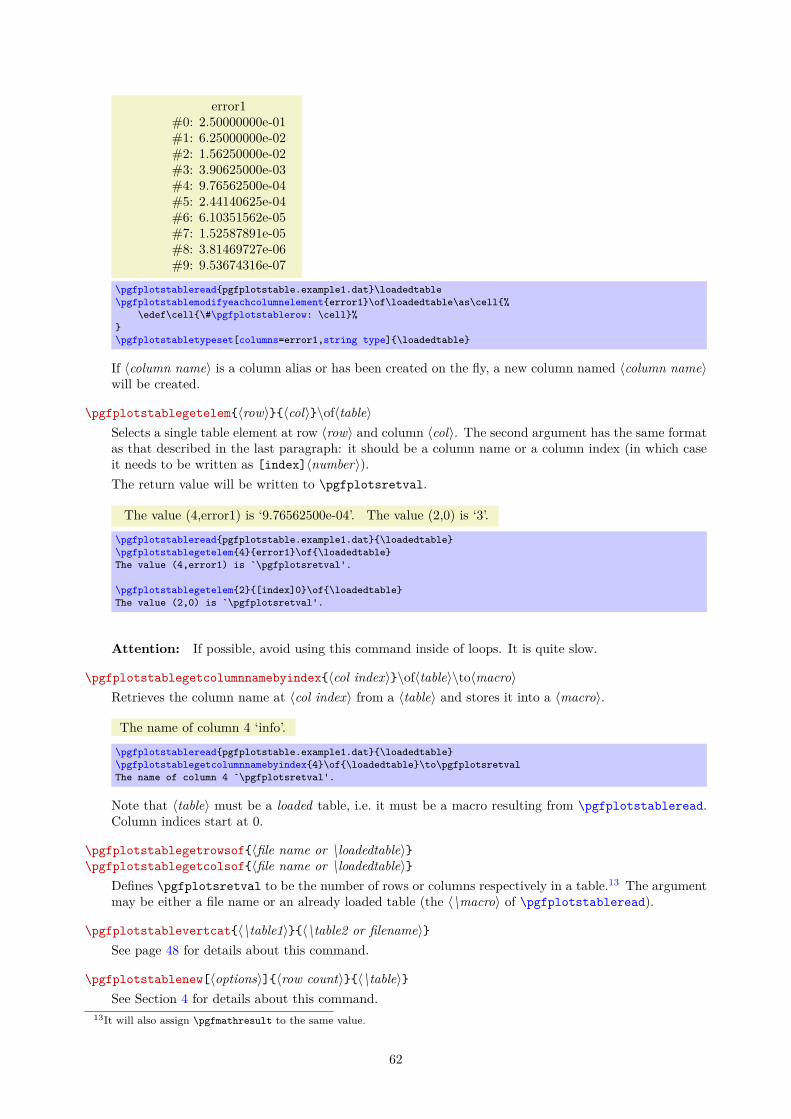
error1#0: 2.50000000e-01#1: 6.25000000e-02#2: 1.56250000e-02#3: 3.90625000e-03#4: 9.76562500e-04#5: 2.44140625e-04#6: 6.10351562e-05#7: 1.52587891e-05#8: 3.81469727e-06#9: 9.53674316e-07

\pgfplotstableread{pgfplotstable.example1.dat}\loadedtable\pgfplotstablemodifyeachcolumnelement{error1}\of\loadedtable\as\cell{%

\edef\cell{\#\pgfplotstablerow: \cell}%}\pgfplotstabletypeset[columns=error1,string type]{\loadedtable}

If 〈column name〉 is a column alias or has been created on the fly, a new column named 〈column name〉will be created.

\pgfplotstablegetelem{〈row〉}{〈col〉}\of〈table〉Selects a single table element at row 〈row〉 and column 〈col〉. The second argument has the same formatas that described in the last paragraph: it should be a column name or a column index (in which caseit needs to be written as [index]〈number〉).The return value will be written to \pgfplotsretval.

The value (4,error1) is ‘9.76562500e-04’. The value (2,0) is ‘3’.

\pgfplotstableread{pgfplotstable.example1.dat}{\loadedtable}\pgfplotstablegetelem{4}{error1}\of{\loadedtable}The value (4,error1) is `\pgfplotsretval'.

\pgfplotstablegetelem{2}{[index]0}\of{\loadedtable}The value (2,0) is `\pgfplotsretval'.

Attention: If possible, avoid using this command inside of loops. It is quite slow.

\pgfplotstablegetcolumnnamebyindex{〈col index〉}\of〈table〉\to〈macro〉Retrieves the column name at 〈col index〉 from a 〈table〉 and stores it into a 〈macro〉.

The name of column 4 ‘info’.

\pgfplotstableread{pgfplotstable.example1.dat}{\loadedtable}\pgfplotstablegetcolumnnamebyindex{4}\of{\loadedtable}\to\pgfplotsretvalThe name of column 4 `\pgfplotsretval'.

Note that 〈table〉 must be a loaded table, i.e. it must be a macro resulting from \pgfplotstableread.Column indices start at 0.

\pgfplotstablegetrowsof{〈file name or \loadedtable〉}\pgfplotstablegetcolsof{〈file name or \loadedtable〉}

Defines \pgfplotsretval to be the number of rows or columns respectively in a table.13 The argumentmay be either a file name or an already loaded table (the 〈\macro〉 of \pgfplotstableread).

\pgfplotstablevertcat{〈\table1〉}{〈\table2 or filename〉}See page 48 for details about this command.

\pgfplotstablenew[〈options〉]{〈row count〉}{〈\table〉}See Section 4 for details about this command.

13It will also assign \pgfmathresult to the same value.

62

\pgfplotstablecreatecol[〈options〉]{〈row count〉}{〈\table〉}See Section 4 for details about this command.

\pgfplotstabletranspose[〈options〉]{〈\outtable〉}{〈\table or filename〉}\pgfplotstabletranspose*[〈options〉]{〈\outtable〉}{〈\table or filename〉}

Defines 〈\outtable〉 to be the transposed of 〈\table of filename〉. The input argument can be either afile name or an already loaded table.The version with ‘*’ is only interesting in conjunction with the columns option, see below.

a b c d0 1 2 34 5 6 78 9 10 1112 13 14 1516 17 18 1920 21 22 23

\pgfplotstabletypeset[string type]{pgfplotstable.example3.dat}

colnames 0 1 2 3 4 5a 0 4 8 12 16 20b 1 5 9 13 17 21c 2 6 10 14 18 22d 3 7 11 15 19 23

\pgfplotstabletranspose\loadedtable{pgfplotstable.example3.dat}\pgfplotstabletypeset[string type]\loadedtable

The optional argument 〈options〉 can contain options which influence the transposition:

/pgfplots/table/colnames from={〈colname〉} (initially empty)Inside of \pgfplotstabletranspose, this key handles how to define output column names.If 〈colname〉 is empty (the initial value), the output column names will simply be the old rowindices, starting with 0.If 〈colname〉 is not empty, it denotes an input column name whose cell values will make up theoutput column names:

colnames 2 6 10 14 18 22a 0 4 8 12 16 20b 1 5 9 13 17 21d 3 7 11 15 19 23

\pgfplotstabletranspose[colnames from=c]\loadedtable{pgfplotstable.example3.dat}\pgfplotstabletypeset[string type]\loadedtable

The argument 〈colname〉 won’t appear as cell contents. It is an error if the cells in 〈colname〉 don’tyield unique column names.

/pgfplots/table/input colnames to={〈name〉} (initially colnames)Inside of \pgfplotstabletranspose, this key handles what to do with input column names.This key will create a further column named 〈name〉 which will be filled with the input columnnames (as string type).

Input 0 1 2 3 4 5a 0 4 8 12 16 20b 1 5 9 13 17 21c 2 6 10 14 18 22d 3 7 11 15 19 23

\pgfplotstabletranspose[input colnames to=Input]\loadedtable{pgfplotstable.example3.dat}\pgfplotstabletypeset[string type]\loadedtable

63

Set 〈name〉 to the empty string to disable this column.

0 1 2 3 4 50 4 8 12 16 201 5 9 13 17 212 6 10 14 18 223 7 11 15 19 23

\pgfplotstabletranspose[input colnames to=]\loadedtable{pgfplotstable.example3.dat}\pgfplotstabletypeset[string type]\loadedtable

/pgfplots/table/columns={〈list〉} (initially empty)Inside of \pgfplotstabletranspose, this key handles which input columns shall be considered forthe transposition.If 〈list〉 is empty, all columns of the input table will be used (which is the initial configuration).If 〈list〉 is not empty, it is expected to be a list of column names. Only these columns will be used asinput for the transposition, just as if the remaining ones weren’t there. It is acceptable to providecolumn aliases or create on use arguments inside of 〈list〉.

colnames 0 1 2 3 4 5a 0 4 8 12 16 20b 1 5 9 13 17 21

\pgfplotstabletranspose[columns={a,b}]\loadedtable{pgfplotstable.example3.dat}\pgfplotstabletypeset[string type]\loadedtable

Here is the only difference between \pgfplotstabletranspose and \pgfplotstabletranspose*:the version without ‘*’ resets the columns key before it starts whereas the version with ‘*’ simplyuses the actual content of columns.

\pgfplotstablesort[〈options〉]〈\resulttable〉〈\table or filename〉Sorts 〈\table or filename〉 according to 〈options〉 and writes the sorted table to 〈\resulttable〉.Use the high level sort key to enable sorting automatically during \pgfplotstabletypeset.

a b c−11 −9 [d]−9 −9 [f]−6 −14 [b]1 13 [g]4 −14 [c]8 −10 [h]11 14 [e]16 18 [i]19 2 [a]19 −6 [j]

\pgfplotstablesort\result{%a b c19 2 [a]-6 -14 [b]4 -14 [c]

-11 -9 [d]11 14 [e]-9 -9 [f]1 13 [g]8 -10 [h]16 18 [i]19 -6 [j]

}\pgfplotstabletypeset[columns/c/.style={string type}]{\result}%

The sort key and comparison function can be customized using the following keys:

/pgfplots/table/sort key={〈column〉} (initially [index]0)Specifies the column which contains the sort key. The argument 〈column〉 can be any of the columnsof the input table, including create on use, alias or [index]〈integer〉 specifications. The initialsetting uses the first available column.

/pgfplots/table/sort key from={〈table〉} (initially empty)Allows to load the sort key from a different 〈table〉, which can be either a 〈\macro〉 or a 〈filename〉.

/pgfplots/table/sort cmp={〈less than routine〉} (initially float <)Allows to use a different comparison function.

64

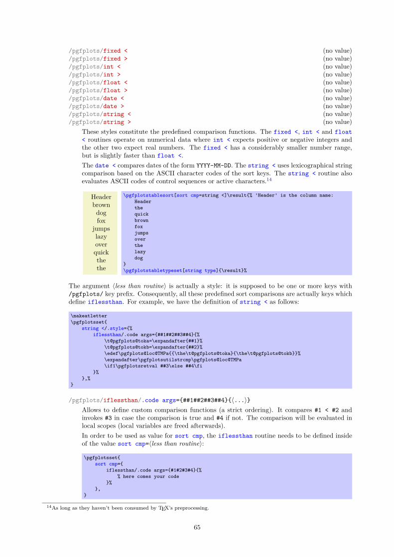
/pgfplots/fixed < (no value)/pgfplots/fixed > (no value)/pgfplots/int < (no value)/pgfplots/int > (no value)/pgfplots/float < (no value)/pgfplots/float > (no value)/pgfplots/date < (no value)/pgfplots/date > (no value)/pgfplots/string < (no value)/pgfplots/string > (no value)

These styles constitute the predefined comparison functions. The fixed <, int < and float< routines operate on numerical data where int < expects positive or negative integers andthe other two expect real numbers. The fixed < has a considerably smaller number range,but is slightly faster than float <.The date < compares dates of the form YYYY-MM-DD. The string < uses lexicographical stringcomparison based on the ASCII character codes of the sort keys. The string < routine alsoevaluates ASCII codes of control sequences or active characters.14

Headerbrowndogfox

jumpslazyoverquickthethe

\pgfplotstablesort[sort cmp=string <]\result{% 'Header' is the column name:Headerthequickbrownfoxjumpsoverthelazydog

}\pgfplotstabletypeset[string type]{\result}%

The argument 〈less than routine〉 is actually a style: it is supposed to be one or more keys with/pgfplots/ key prefix. Consequently, all these predefined sort comparisons are actually keys whichdefine iflessthan. For example, we have the definition of string < as follows:

\makeatletter\pgfplotsset{

string </.style={%iflessthan/.code args={##1##2##3##4}{%

\t@pgfplots@toka=\expandafter{##1}%\t@pgfplots@tokb=\expandafter{##2}%\edef\pgfplots@loc@TMPa{{\the\t@pgfplots@toka}{\the\t@pgfplots@tokb}}%\expandafter\pgfplotsutilstrcmp\pgfplots@loc@TMPa\if1\pgfplotsretval ##3\else ##4\fi

}%},%

}

/pgfplots/iflessthan/.code args={##1##2##3##4}{〈...〉}Allows to define custom comparison functions (a strict ordering). It compares #1 < #2 andinvokes #3 in case the comparison is true and #4 if not. The comparison will be evaluated inlocal scopes (local variables are freed afterwards).In order to be used as value for sort cmp, the iflessthan routine needs to be defined insideof the value sort cmp=〈less than routine〉:

\pgfplotsset{sort cmp={

iflessthan/.code args={#1#2#3#4}{%% here comes your code

}%},

}

14As long as they haven’t been consumed by TEX’s preprocessing.

65

5.6 Repeating Things: Loops\foreach〈variables〉 in 〈list〉 {〈commands〉}

A powerful loop command provided by TikZ, see [2, Section “Utilities”].

Iterating 1. Iterating 2. Iterating 3. Iterating 4.

\foreach \x in {1,2,...,4} {Iterating \x. }%

A pgfplots related example could be

\foreach \i in {1,2,...,10} {\addplot table {datafile\i}; }%

The following loop commands come with pgfplots. They are similar to the powerful TikZ \foreach loopcommand, which, however, is not always useful for table processing: the effect of its loop body end aftereach iteration.

The following pgfplots looping macros are an alternative.

\pgfplotsforeachungrouped〈variable〉 in 〈list〉 {〈command〉}A specialized variant of \foreach which can do two things: it does not introduce extra groups whileexecuting 〈command〉 and it allows to invoke the math parser for (simple!) 〈x0〉,〈x1〉,...,〈xn〉 expres-sions.

Iterating 1. Iterating 2. Iterating 3. Iterating 4. All collected = , 1, 2, 3, 4.

\def\allcollected{}\pgfplotsforeachungrouped \x in {1,2,...,4} {Iterating \x. \edef\allcollected{\allcollected, \x}}%All collected = \allcollected.

A more useful example might be to work with tables:

\pgfplotsforeachungrouped \i in {1,2,...,10} {%\pgfplotstablevertcat{\output}{datafile\i} % appends `datafile\i' -> `\output'

}%% since it was ungrouped, \output is still defined (would not work% with \foreach)

Remark: The special syntax 〈list〉=〈x0〉,〈x1〉,...,〈xn〉, i.e. with two leading elements, followed bydots and a final element, invokes the math parser for the loop. Thus, it allows larger number rangesthan any other syntax if /pgf/fpu is active. In all other cases, \pgfplotsforeachungrouped invokes\foreach and provides the results without TEX groups.

\pgfplotsinvokeforeach{〈list〉} {〈command〉}A variant of \pgfplotsforeachungrouped (and such also of \foreach) which replaces any occurrenceof #1 inside of 〈command〉 once for every element in 〈list〉. Thus, it actually assumes that 〈command〉is like a \newcommand body.In other words, 〈command〉 is invoked for every element of 〈list〉. The actual element of 〈list〉 is availableas #1.As \pgfplotsforeachungrouped, this command does not introduce extra scopes (i.e. it is ungroupedas well).The difference to \foreach \x in 〈list〉{〈command〉} is subtle: the \x would not be expanded whereas#1 is.

Invoke them: [a] [b] [c] [d]

\pgfkeys{otherstyle a/.code={[a]},otherstyle b/.code={[b]},otherstyle c/.code={[c]},otherstyle d/.code={[d]}}

\pgfplotsinvokeforeach{a,b,c,d}{\pgfkeys{key #1/.style={otherstyle #1}}}

Invoke them: \pgfkeys{key a} \pgfkeys{key b} \pgfkeys{key c} \pgfkeys{key d}

66

The counterexample would use a macro (here \x) as loop argument:

Invoke them: [d] [d] [d] [d]

\pgfkeys{otherstyle a/.code={[a]},otherstyle b/.code={[b]},otherstyle c/.code={[c]},otherstyle d/.code={[d]}}

\pgfplotsforeachungrouped \x in {a,b,c,d}{\pgfkeys{key \x/.style={otherstyle \x}}}

Invoke them: \pgfkeys{key a} \pgfkeys{key b} \pgfkeys{key c} \pgfkeys{key d}

Restrictions: You cannot nest this command yet (since it does not introduce protection by scopes).

67

Index— Symbols —1000 sep key . . . . . . . . . . . . . . . . . . . . . . . . . . . 331000 sep in fractionals key . . . . . . . . . . . . . . 33

— A —.add handler . . . . . . . . . . . . . . . . . . . . . . . . . . . . 60after row key . . . . . . . . . . . . . . . . . . . . . . . . . . . 19alias key . . . . . . . . . . . . . . . . . . . . . . . . . . . . . . 10.append code handler . . . . . . . . . . . . . . . . . . . . . 60.append style handler . . . . . . . . . . . . . . . . . . . . 60assign cell content key . . . . . . . . . . . . . . . . . . 37assign column name key . . . . . . . . . . . . . . . . . . . 12assume math mode key . . . . . . . . . . . . . . . . . . . . 36

— B —before row key . . . . . . . . . . . . . . . . . . . . . . . . . . 17begin table key . . . . . . . . . . . . . . . . . . . . . . . . . 23

— C —clear infinite key . . . . . . . . . . . . . . . . . . . . . . 41.code handler . . . . . . . . . . . . . . . . . . . . . . . . . . . 60.code 2 args handler . . . . . . . . . . . . . . . . . . . . . 60col sep key . . . . . . . . . . . . . . . . . . . . . . . . . . . . . 5colnames from key . . . . . . . . . . . . . . . . . . . . . . . 63column name key . . . . . . . . . . . . . . . . . . . . . . . . . 12column type key . . . . . . . . . . . . . . . . . . . . . . . . . 11columns key . . . . . . . . . . . . . . . . . . . . . . . . . 10, 64comment chars key . . . . . . . . . . . . . . . . . . . . . . . . 8copy key . . . . . . . . . . . . . . . . . . . . . . . . . . . . . . . 51copy column from table key . . . . . . . . . . . . . . . 52create on use key . . . . . . . . . . . . . . . . . . . . . . . 50

— D —date < key . . . . . . . . . . . . . . . . . . . . . . . . . . . . . 65date > key . . . . . . . . . . . . . . . . . . . . . . . . . . . . . 65date type key . . . . . . . . . . . . . . . . . . . . . . . . . . . 38\day . . . . . . . . . . . . . . . . . . . . . . . . . . . . . . . . . . 39dcolumn key . . . . . . . . . . . . . . . . . . . . . . . . . . . . 14debug key . . . . . . . . . . . . . . . . . . . . . . . . . . . . . . 25dec sep key . . . . . . . . . . . . . . . . . . . . . . . . . . . . 33dec sep align key . . . . . . . . . . . . . . . . . . . . . . . 13disable rowcol styles key . . . . . . . . . . . . . . . . 59display columns key . . . . . . . . . . . . . . . . . . . . . 11divide by key . . . . . . . . . . . . . . . . . . . . . . . . . . . 41dyadic refinement rate key . . . . . . . . . . . . . . . 54

— E —empty cells with key . . . . . . . . . . . . . . . . . . . . 46end table key . . . . . . . . . . . . . . . . . . . . . . . . . . . 24every col no 〈index〉 key . . . . . . . . . . . . . . . . . 11every column key . . . . . . . . . . . . . . . . . . . . . . . . 16every even column key . . . . . . . . . . . . . . . . . . . . 15every even row key . . . . . . . . . . . . . . . . . . . . . . 19every first column key . . . . . . . . . . . . . . . . . . . 15every first row key . . . . . . . . . . . . . . . . . . . . . 21every head row key . . . . . . . . . . . . . . . . . . . . . . 20every last column key . . . . . . . . . . . . . . . . . . . . 15every last row key . . . . . . . . . . . . . . . . . . . . . . 21every nth row key . . . . . . . . . . . . . . . . . . . . . . . 21every odd column key . . . . . . . . . . . . . . . . . . . . 16every odd row key . . . . . . . . . . . . . . . . . . . . . . . 20

every relative key . . . . . . . . . . . . . . . . . . . . . . 30every row 〈rowindex〉 column 〈colindex〉 key . . 22every row 〈rowindex〉 column 〈colname〉 key . . . 22every row no 〈index〉 key . . . . . . . . . . . . . . . . . 21every row no 〈rowindex〉 column no 〈colindex〉

key . . . . . . . . . . . . . . . . . . . . . . . . . . . . . 22every table key . . . . . . . . . . . . . . . . . . . . . . . . . 23exponent key . . . . . . . . . . . . . . . . . . . . . . . . . . . 36expr key . . . . . . . . . . . . . . . . . . . . . . . . . . . . 41, 52expr accum key . . . . . . . . . . . . . . . . . . . . . . . . . . 53

— F —fixed key . . . . . . . . . . . . . . . . . . . . . . . . . . . . . . 27fixed < key . . . . . . . . . . . . . . . . . . . . . . . . . . . . 65fixed > key . . . . . . . . . . . . . . . . . . . . . . . . . . . . 65fixed relative key . . . . . . . . . . . . . . . . . . . . . . 30fixed zerofill key . . . . . . . . . . . . . . . . . . . . . . 27float < key . . . . . . . . . . . . . . . . . . . . . . . . . . . . 65float > key . . . . . . . . . . . . . . . . . . . . . . . . . . . . 65Floating Point Unit . . . . . . . . . . . . . . . . . . . . . . . 53font key . . . . . . . . . . . . . . . . . . . . . . . . . . . . . . . 23fonts by sign key . . . . . . . . . . . . . . . . . . . . . . . 46force remake key . . . . . . . . . . . . . . . . . . . . . . . . 25\foreach . . . . . . . . . . . . . . . . . . . . . . . . . . . . . . . 66format key . . . . . . . . . . . . . . . . . . . . . . . . . . . . . . 7fpu key . . . . . . . . . . . . . . . . . . . . . . . . . . . . . . . . 52frac key . . . . . . . . . . . . . . . . . . . . . . . . . . . . . . . 31frac denom key . . . . . . . . . . . . . . . . . . . . . . . . . . 31frac shift key . . . . . . . . . . . . . . . . . . . . . . . . . . 32frac TeX key . . . . . . . . . . . . . . . . . . . . . . . . . . . 31frac whole key . . . . . . . . . . . . . . . . . . . . . . . . . . 32function graph cut x key . . . . . . . . . . . . . . . . . 58function graph cut y key . . . . . . . . . . . . . . . . . 56

— G —gradient key . . . . . . . . . . . . . . . . . . . . . . . . . . . 55gradient loglog key . . . . . . . . . . . . . . . . . . . . . 55gradient semilogx key . . . . . . . . . . . . . . . . . . . . 55gradient semilogy key . . . . . . . . . . . . . . . . . . . . 55

— H —header key . . . . . . . . . . . . . . . . . . . . . . . . . . . . . . 6

— I —idyadic refinement rate key . . . . . . . . . . . . . . 55iflessthan key . . . . . . . . . . . . . . . . . . . . . . . . . . 65ignore chars key . . . . . . . . . . . . . . . . . . . . . . . . . 7implicit . key . . . . . . . . . . . . . . . . . . . . . . . . . . 9include outfiles key . . . . . . . . . . . . . . . . . . . . 25.initial handler . . . . . . . . . . . . . . . . . . . . . . . . 60input colnames to key . . . . . . . . . . . . . . . . . . . . 63int < key . . . . . . . . . . . . . . . . . . . . . . . . . . . . . . 65int > key . . . . . . . . . . . . . . . . . . . . . . . . . . . . . . 65int detect key . . . . . . . . . . . . . . . . . . . . . . . . . . 30int trunc key . . . . . . . . . . . . . . . . . . . . . . . . . . . 31iquotient key . . . . . . . . . . . . . . . . . . . . . . . . . . . 54

— K —Key handlers

.add . . . . . . . . . . . . . . . . . . . . . . . . . . . . . . 60

.append code . . . . . . . . . . . . . . . . . . . . . . . 60

68

.append style . . . . . . . . . . . . . . . . . . . . . . 60

.code . . . . . . . . . . . . . . . . . . . . . . . . . . . . . 60

.code 2 args . . . . . . . . . . . . . . . . . . . . . . . 60

.initial . . . . . . . . . . . . . . . . . . . . . . . . . . . 60

.style . . . . . . . . . . . . . . . . . . . . . . . . . . . . . 59

— L —linear regression key . . . . . . . . . . . . . . . . . . . . 56longtable . . . . . . . . . . . . . . . . . . . . . . . . . . . . . . . 23

— M —mantissa sep key . . . . . . . . . . . . . . . . . . . . . . . . 35min exponent for 1000 sep key . . . . . . . . . . . . . 34\month . . . . . . . . . . . . . . . . . . . . . . . . . . . . . . . . 39\monthname . . . . . . . . . . . . . . . . . . . . . . . . . . . . . 39\monthshortname . . . . . . . . . . . . . . . . . . . . . . . . 39Multi-page . . . . . . . . . . . . . . . . . . . . . . . . . . . . . 23multicolumn names key . . . . . . . . . . . . . . . . . . . . 12multiply -1 key . . . . . . . . . . . . . . . . . . . . . . . . . 42multiply by key . . . . . . . . . . . . . . . . . . . . . . . . . 41multirow . . . . . . . . . . . . . . . . . . . . . . . . . . . . . . . 38

— N —\newcolumntype . . . . . . . . . . . . . . . . . . . . . . . . . 26numeric as string type key . . . . . . . . . . . . . . . 38numeric type key . . . . . . . . . . . . . . . . . . . . . . . . 38

— O —outfile key . . . . . . . . . . . . . . . . . . . . . . . . . 24, 58output empty row key . . . . . . . . . . . . . . . . . . . . 22

— P —percent is letter key . . . . . . . . . . . . . . . . . . . . . 8/pgf/

fpu . . . . . . . . . . . . . . . . . . . . . . . . . . . . . . . 52number format/

1000 sep . . . . . . . . . . . . . . . . . . . . . . . . . 331000 sep in fractionals . . . . . . . . . . . . 33assume math mode . . . . . . . . . . . . . . . . . . 36dec sep . . . . . . . . . . . . . . . . . . . . . . . . . . 33every relative . . . . . . . . . . . . . . . . . . . . 30fixed . . . . . . . . . . . . . . . . . . . . . . . . . . . . 27fixed relative . . . . . . . . . . . . . . . . . . . . 30fixed zerofill . . . . . . . . . . . . . . . . . . . . 27frac . . . . . . . . . . . . . . . . . . . . . . . . . . . . 31frac denom . . . . . . . . . . . . . . . . . . . . . . . 31frac shift . . . . . . . . . . . . . . . . . . . . . . . 32frac TeX . . . . . . . . . . . . . . . . . . . . . . . . . 31frac whole . . . . . . . . . . . . . . . . . . . . . . . 32int detect . . . . . . . . . . . . . . . . . . . . . . . 30int trunc . . . . . . . . . . . . . . . . . . . . . . . . 31min exponent for 1000 sep . . . . . . . . . . 34precision . . . . . . . . . . . . . . . . . . . . . . . . 32print sign . . . . . . . . . . . . . . . . . . . . . . . 35read comma as period . . . . . . . . . . . . . . 32relative style . . . . . . . . . . . . . . . . . . . . 30relative* . . . . . . . . . . . . . . . . . . . . . . . . 29retain unit mantissa . . . . . . . . . . . . . . 36sci . . . . . . . . . . . . . . . . . . . . . . . . . . . . . 28sci 10^e . . . . . . . . . . . . . . . . . . . . . . . . . 35sci 10e . . . . . . . . . . . . . . . . . . . . . . . . . . 35sci E . . . . . . . . . . . . . . . . . . . . . . . . . . . . 35sci e . . . . . . . . . . . . . . . . . . . . . . . . . . . . 35sci generic . . . . . . . . . . . . . . . . . . . . . . 35

sci precision . . . . . . . . . . . . . . . . . . . . . 32sci subscript . . . . . . . . . . . . . . . . . . . . . 35sci superscript . . . . . . . . . . . . . . . . . . . 35sci zerofill . . . . . . . . . . . . . . . . . . . . . 28set decimal separator . . . . . . . . . . . . . . 32set thousands separator . . . . . . . . . . . . 33showpos . . . . . . . . . . . . . . . . . . . . . . . . . . 35skip 0. . . . . . . . . . . . . . . . . . . . . . . . . . . 34std . . . . . . . . . . . . . . . . . . . . . . . . . . . . . 28use comma . . . . . . . . . . . . . . . . . . . . . . . . 34use period . . . . . . . . . . . . . . . . . . . . . . . 34verbatim . . . . . . . . . . . . . . . . . . . . . . . . . 36zerofill . . . . . . . . . . . . . . . . . . . . . . . . . 28

\pgfmathifisint . . . . . . . . . . . . . . . . . . . . . . . . 31\pgfmathprintnumber . . . . . . . . . . . . . . . . . . . . . 27\pgfmathprintnumberto . . . . . . . . . . . . . . . . . . . 27\pgfplotsforeachungrouped . . . . . . . . . . . . . . . . 66\pgfplotsinvokeforeach . . . . . . . . . . . . . . . . . . 66\pgfplotstableclear . . . . . . . . . . . . . . . . . . . . . 48\pgfplotstablecol . . . . . . . . . . . . . . . . . . . . . . . 16\pgfplotstablecolname . . . . . . . . . . . . . . . . . . . 16\pgfplotstablecols . . . . . . . . . . . . . . . . . . . . . . 17\pgfplotstablecreatecol . . . . . . . . . . . . . . 48, 63\pgfplotstableforeachcolumn . . . . . . . . . . . . . . 61\pgfplotstableforeachcolumnelement . . . . . . . . 61\pgfplotstablegetcolsof . . . . . . . . . . . . . . . . . 62\pgfplotstablegetcolumnnamebyindex . . . . . . . . 62\pgfplotstablegetelem . . . . . . . . . . . . . . . . . . . 62\pgfplotstablegetrowsof . . . . . . . . . . . . . . . . . 62\pgfplotstablemodifyeachcolumnelement . . . . . 61\pgfplotstablename . . . . . . . . . . . . . . . . . . . . . . 17\pgfplotstablenew . . . . . . . . . . . . . . . . . . . . 47, 62\pgfplotstableread . . . . . . . . . . . . . . . . . . . . . . . 4\pgfplotstablerow . . . . . . . . . . . . . . . . . . . . . . . 16\pgfplotstablerows . . . . . . . . . . . . . . . . . . . . . . 17\pgfplotstablesave . . . . . . . . . . . . . . . . . . . . . . 58\pgfplotstableset . . . . . . . . . . . . . . . . . . . . . . . . 2\pgfplotstablesort . . . . . . . . . . . . . . . . . . . . . . 64\pgfplotstabletranspose . . . . . . . . . . . . . . . . . 63\pgfplotstabletypeset . . . . . . . . . . . . . . . . . . . . 3\pgfplotstabletypesetfile . . . . . . . . . . . . . . . . . 4\pgfplotstablevertcat . . . . . . . . . . . . . . . . 48, 62postproc cell content key . . . . . . . . . . . . . . . . 45Precision . . . . . . . . . . . . . . . . . . . . . . . . . . . . . . 52f.precision key . . . . . . . . . . . . . . . . . . . . . . . . . . . 32preproc cell content key . . . . . . . . . . . . . . . . . 40print sign key . . . . . . . . . . . . . . . . . . . . . . . . . . 35

— Q —quotient key . . . . . . . . . . . . . . . . . . . . . . . . . . . 54

— R —read comma as period key . . . . . . . . . . . . . . . . . 32relative style key . . . . . . . . . . . . . . . . . . . . . . 30relative* key . . . . . . . . . . . . . . . . . . . . . . . . . . . 29Replicate headers . . . . . . . . . . . . . . . . . . . . . . . . 23reset styles key . . . . . . . . . . . . . . . . . . . . . . . . 59retain unit mantissa key . . . . . . . . . . . . . . . . . 36row predicate key . . . . . . . . . . . . . . . . . . . . . . . 42row sep key . . . . . . . . . . . . . . . . . . . . . . . . . . . . . 7

— S —sci key . . . . . . . . . . . . . . . . . . . . . . . . . . . . . . . . 28sci 10^e key . . . . . . . . . . . . . . . . . . . . . . . . . . . 35

69

sci 10e key . . . . . . . . . . . . . . . . . . . . . . . . . . . . 35sci E key . . . . . . . . . . . . . . . . . . . . . . . . . . . . . . 35sci e key . . . . . . . . . . . . . . . . . . . . . . . . . . . . . . 35sci generic key . . . . . . . . . . . . . . . . . . . . . . . . . 35sci precision key . . . . . . . . . . . . . . . . . . . . . . . 32sci sep align key . . . . . . . . . . . . . . . . . . . . . . . 14sci subscript key . . . . . . . . . . . . . . . . . . . . . . . 35sci superscript key . . . . . . . . . . . . . . . . . . . . . 35sci zerofill key . . . . . . . . . . . . . . . . . . . . . . . . 28search path key . . . . . . . . . . . . . . . . . . . . . . . . . . 9select equal part entry of key . . . . . . . . . . . . 43set key . . . . . . . . . . . . . . . . . . . . . . . . . . . . . . . . 51set content key . . . . . . . . . . . . . . . . . . . . . . . . . 46set decimal separator key . . . . . . . . . . . . . . . . 32set list key . . . . . . . . . . . . . . . . . . . . . . . . . . . 51set thousands separator key . . . . . . . . . . . . . . 33showpos key . . . . . . . . . . . . . . . . . . . . . . . . . . . . 35skip 0. key . . . . . . . . . . . . . . . . . . . . . . . . . . . . 34skip coltypes key . . . . . . . . . . . . . . . . . . . . . . . 25skip first n key . . . . . . . . . . . . . . . . . . . . . . . . . 9skip rows between index key . . . . . . . . . . . . . . 43sort key . . . . . . . . . . . . . . . . . . . . . . . . . . . . . . . 14sort cmp key . . . . . . . . . . . . . . . . . . . . . . . . . . . 64sort key key . . . . . . . . . . . . . . . . . . . . . . . . . . . 64sort key from key . . . . . . . . . . . . . . . . . . . . . . . 64sqrt key . . . . . . . . . . . . . . . . . . . . . . . . . . . . . . . 41std key . . . . . . . . . . . . . . . . . . . . . . . . . . . . . . . . 28string < key . . . . . . . . . . . . . . . . . . . . . . . . . . . 65string > key . . . . . . . . . . . . . . . . . . . . . . . . . . . 65string replace key . . . . . . . . . . . . . . . . . . . . . . 40string replace* key . . . . . . . . . . . . . . . . . . . . . 40string type key . . . . . . . . . . . . . . . . . . . . . . . . . 38.style handler . . . . . . . . . . . . . . . . . . . . . . . . . . 59

— T —table/

after row . . . . . . . . . . . . . . . . . . . . . . . . . . 19alias . . . . . . . . . . . . . . . . . . . . . . . . . . . . . 10assign cell content . . . . . . . . . . . . . . . . . 37assign column name . . . . . . . . . . . . . . . . . . 12before row . . . . . . . . . . . . . . . . . . . . . . . . . 17begin table . . . . . . . . . . . . . . . . . . . . . . . . 23clear infinite . . . . . . . . . . . . . . . . . . . . . . 41col sep . . . . . . . . . . . . . . . . . . . . . . . . . . . . . 5colnames from . . . . . . . . . . . . . . . . . . . . . . 63column name . . . . . . . . . . . . . . . . . . . . . . . . 12column type . . . . . . . . . . . . . . . . . . . . . . . . 11columns . . . . . . . . . . . . . . . . . . . . . . . . . 10, 64comment chars . . . . . . . . . . . . . . . . . . . . . . . 8create col/

copy . . . . . . . . . . . . . . . . . . . . . . . . . . . . 51copy column from table . . . . . . . . . . . . . 52dyadic refinement rate . . . . . . . . . . . . . 54expr . . . . . . . . . . . . . . . . . . . . . . . . . . . . 52expr accum . . . . . . . . . . . . . . . . . . . . . . . 53function graph cut x . . . . . . . . . . . . . . 58function graph cut y . . . . . . . . . . . . . . 56gradient . . . . . . . . . . . . . . . . . . . . . . . . . 55gradient loglog . . . . . . . . . . . . . . . . . . . 55gradient semilogx . . . . . . . . . . . . . . . . . 55gradient semilogy . . . . . . . . . . . . . . . . . 55idyadic refinement rate . . . . . . . . . . . . 55iquotient . . . . . . . . . . . . . . . . . . . . . . . . 54linear regression . . . . . . . . . . . . . . . . . 56

quotient . . . . . . . . . . . . . . . . . . . . . . . . . 54set . . . . . . . . . . . . . . . . . . . . . . . . . . . . . 51set list . . . . . . . . . . . . . . . . . . . . . . . . . 51

create on use . . . . . . . . . . . . . . . . . . . . . . 50date type . . . . . . . . . . . . . . . . . . . . . . . . . . 38dcolumn . . . . . . . . . . . . . . . . . . . . . . . . . . . . 14debug . . . . . . . . . . . . . . . . . . . . . . . . . . . . . 25dec sep align . . . . . . . . . . . . . . . . . . . . . . 13disable rowcol styles . . . . . . . . . . . . . . . 59display columns . . . . . . . . . . . . . . . . . . . . . 11divide by . . . . . . . . . . . . . . . . . . . . . . . . . . 41empty cells with . . . . . . . . . . . . . . . . . . . . 46end table . . . . . . . . . . . . . . . . . . . . . . . . . . 24every col no 〈index〉 . . . . . . . . . . . . . . . . . 11every column . . . . . . . . . . . . . . . . . . . . . . . 16every even column . . . . . . . . . . . . . . . . . . . 15every even row . . . . . . . . . . . . . . . . . . . . . . 19every first column . . . . . . . . . . . . . . . . . . 15every first row . . . . . . . . . . . . . . . . . . . . . 21every head row . . . . . . . . . . . . . . . . . . . . . . 20every last column . . . . . . . . . . . . . . . . . . . 15every last row . . . . . . . . . . . . . . . . . . . . . . 21every nth row . . . . . . . . . . . . . . . . . . . . . . 21every odd column . . . . . . . . . . . . . . . . . . . . 16every odd row . . . . . . . . . . . . . . . . . . . . . . 20every row 〈rowindex〉 column 〈colindex〉 . 22every row 〈rowindex〉 column 〈colname〉 . . 22every row no 〈index〉 . . . . . . . . . . . . . . . . . 21every row no 〈rowindex〉 column no

〈colindex〉 . . . . . . . . . . . . . . . . . . . . . . . . 22every table . . . . . . . . . . . . . . . . . . . . . . . . 23font . . . . . . . . . . . . . . . . . . . . . . . . . . . . . . 23fonts by sign . . . . . . . . . . . . . . . . . . . . . . 46force remake . . . . . . . . . . . . . . . . . . . . . . . 25format . . . . . . . . . . . . . . . . . . . . . . . . . . . . . . 7header . . . . . . . . . . . . . . . . . . . . . . . . . . . . . . 6ignore chars . . . . . . . . . . . . . . . . . . . . . . . . 7include outfiles . . . . . . . . . . . . . . . . . . . . 25input colnames to . . . . . . . . . . . . . . . . . . . 63multicolumn names . . . . . . . . . . . . . . . . . . . 12multiply -1 . . . . . . . . . . . . . . . . . . . . . . . . 42multiply by . . . . . . . . . . . . . . . . . . . . . . . . 41numeric as string type . . . . . . . . . . . . . . . 38numeric type . . . . . . . . . . . . . . . . . . . . . . . 38outfile . . . . . . . . . . . . . . . . . . . . . . . . . 24, 58output empty row . . . . . . . . . . . . . . . . . . . . 22percent is letter . . . . . . . . . . . . . . . . . . . . 8postproc cell content . . . . . . . . . . . . . . . 45preproc/

expr . . . . . . . . . . . . . . . . . . . . . . . . . . . . 41preproc cell content . . . . . . . . . . . . . . . . 40reset styles . . . . . . . . . . . . . . . . . . . . . . . 59row predicate . . . . . . . . . . . . . . . . . . . . . . 42row sep . . . . . . . . . . . . . . . . . . . . . . . . . . . . . 7sci sep align . . . . . . . . . . . . . . . . . . . . . . 14search path/

implicit . . . . . . . . . . . . . . . . . . . . . . . . . 9search path . . . . . . . . . . . . . . . . . . . . . . . . . 9select equal part entry of . . . . . . . . . . . 43set content . . . . . . . . . . . . . . . . . . . . . . . . 46skip coltypes . . . . . . . . . . . . . . . . . . . . . . 25skip first n . . . . . . . . . . . . . . . . . . . . . . . . 9skip rows between index . . . . . . . . . . . . . . 43

70

sort . . . . . . . . . . . . . . . . . . . . . . . . . . . . . . 14sort cmp . . . . . . . . . . . . . . . . . . . . . . . . . . . 64sort key . . . . . . . . . . . . . . . . . . . . . . . . . . . 64sort key from . . . . . . . . . . . . . . . . . . . . . . 64sqrt . . . . . . . . . . . . . . . . . . . . . . . . . . . . . . 41string replace . . . . . . . . . . . . . . . . . . . . . . 40string replace* . . . . . . . . . . . . . . . . . . . . . 40string type . . . . . . . . . . . . . . . . . . . . . . . . 38TeX comment . . . . . . . . . . . . . . . . . . . . . . . . 25text indicator . . . . . . . . . . . . . . . . . . . . . . . 9text special chars . . . . . . . . . . . . . . . . . . . 8trim cells . . . . . . . . . . . . . . . . . . . . . . . . . . 6typeset . . . . . . . . . . . . . . . . . . . . . . . . . . . . 25typeset cell . . . . . . . . . . . . . . . . . . . . . . . 24unique . . . . . . . . . . . . . . . . . . . . . . . . . . . . . 44verb string type . . . . . . . . . . . . . . . . . . . . 38white space chars . . . . . . . . . . . . . . . . . . . . 8write to macro . . . . . . . . . . . . . . . . . . . . . . 25

TeX comment key . . . . . . . . . . . . . . . . . . . . . . . . . 25text indicator key . . . . . . . . . . . . . . . . . . . . . . . 9text special chars key . . . . . . . . . . . . . . . . . . . . 8trim cells key . . . . . . . . . . . . . . . . . . . . . . . . . . . 6typeset key . . . . . . . . . . . . . . . . . . . . . . . . . . . . 25typeset cell key . . . . . . . . . . . . . . . . . . . . . . . . 24

— U —unique key . . . . . . . . . . . . . . . . . . . . . . . . . . . . . 44use comma key . . . . . . . . . . . . . . . . . . . . . . . . . . . 34use period key . . . . . . . . . . . . . . . . . . . . . . . . . . 34

— V —verb string type key . . . . . . . . . . . . . . . . . . . . 38verbatim key . . . . . . . . . . . . . . . . . . . . . . . . . . . 36

— W —\weekday . . . . . . . . . . . . . . . . . . . . . . . . . . . . . . . 39\weekdayname . . . . . . . . . . . . . . . . . . . . . . . . . . . 39\weekdayshortname . . . . . . . . . . . . . . . . . . . . . . . 39white space chars key . . . . . . . . . . . . . . . . . . . . . 8write to macro key . . . . . . . . . . . . . . . . . . . . . . 25

— Y —\year . . . . . . . . . . . . . . . . . . . . . . . . . . . . . . . . . 39

— Z —zerofill key . . . . . . . . . . . . . . . . . . . . . . . . . . . 28

71

References[1] D. Knuth. Computers & Typesetting. Addison Wesley, 2000.

[2] T. Tantau. TikZ and pgf manual. http://sourceforge.net/projects/pgf. v. ≥ 2.00.

[3] J. Wright and C. Feuersänger. Implementing keyval input: an introduction. http://pgfplots.sourceforge.net as .pdf, 2008.

72

http://sourceforge.net/projects/pgf

http://pgfplots.sourceforge.net

http://pgfplots.sourceforge.net

http://www.morningstar2.demon.co.uk/papers/keyval.pdf

package pgfplots manual - ctan.math.washington.edu

Documents