package 'smooth

Package ‘smooth’March 6, 2018

Type Package

Title Forecasting Using Smoothing Functions

Version 2.4.1

Date 2018-03-04

URL https://github.com/config-i1/smooth

BugReports https://github.com/config-i1/smooth/issues

DescriptionFunctions implementing Single Source of Error state-space models for purposes of time seriesanalysis and forecasting. The package includes exponential smoothing, SARIMA in state-space forms andseveral simulation functions.

License GPL (>= 2)

Depends R (>= 3.0.2)

Imports Rcpp (>= 0.12.3), stats, graphics, forecast, nloptr, utils,zoo

LinkingTo Rcpp, RcppArmadillo (>= 0.8.100.0.0)

Suggests Mcomp, numDeriv, testthat, knitr, rmarkdown

VignetteBuilder knitr

RoxygenNote 6.0.1

NeedsCompilation yes

Author Ivan Svetunkov [aut, cre] (Lecturer at Centre for Marketing Analyticsand Forecasting, Lancaster University, UK)

Maintainer Ivan Svetunkov <[email protected]>

Repository CRAN

Date/Publication 2018-03-06 07:33:59 UTC

1

https://github.com/config-i1/smooth

https://github.com/config-i1/smooth/issues

2 Accuracy

R topics documented:

Accuracy . . . . . . . . . . . . . . . . . . . . . . . . . . . . . . . . . . . . . . . . . . 2AICc . . . . . . . . . . . . . . . . . . . . . . . . . . . . . . . . . . . . . . . . . . . . . 4auto.ces . . . . . . . . . . . . . . . . . . . . . . . . . . . . . . . . . . . . . . . . . . . 5auto.ges . . . . . . . . . . . . . . . . . . . . . . . . . . . . . . . . . . . . . . . . . . . 8auto.ssarima . . . . . . . . . . . . . . . . . . . . . . . . . . . . . . . . . . . . . . . . . 11ces . . . . . . . . . . . . . . . . . . . . . . . . . . . . . . . . . . . . . . . . . . . . . . 15es . . . . . . . . . . . . . . . . . . . . . . . . . . . . . . . . . . . . . . . . . . . . . . 20forecast.smooth . . . . . . . . . . . . . . . . . . . . . . . . . . . . . . . . . . . . . . . 27ges . . . . . . . . . . . . . . . . . . . . . . . . . . . . . . . . . . . . . . . . . . . . . . 29graphmaker . . . . . . . . . . . . . . . . . . . . . . . . . . . . . . . . . . . . . . . . . 34hm . . . . . . . . . . . . . . . . . . . . . . . . . . . . . . . . . . . . . . . . . . . . . . 35iss . . . . . . . . . . . . . . . . . . . . . . . . . . . . . . . . . . . . . . . . . . . . . . 36MPE . . . . . . . . . . . . . . . . . . . . . . . . . . . . . . . . . . . . . . . . . . . . . 38nParam . . . . . . . . . . . . . . . . . . . . . . . . . . . . . . . . . . . . . . . . . . . 40orders . . . . . . . . . . . . . . . . . . . . . . . . . . . . . . . . . . . . . . . . . . . . 41pls . . . . . . . . . . . . . . . . . . . . . . . . . . . . . . . . . . . . . . . . . . . . . . 43pointLik . . . . . . . . . . . . . . . . . . . . . . . . . . . . . . . . . . . . . . . . . . . 44sim.ces . . . . . . . . . . . . . . . . . . . . . . . . . . . . . . . . . . . . . . . . . . . 45sim.es . . . . . . . . . . . . . . . . . . . . . . . . . . . . . . . . . . . . . . . . . . . . 47sim.ges . . . . . . . . . . . . . . . . . . . . . . . . . . . . . . . . . . . . . . . . . . . 50sim.sma . . . . . . . . . . . . . . . . . . . . . . . . . . . . . . . . . . . . . . . . . . . 52sim.ssarima . . . . . . . . . . . . . . . . . . . . . . . . . . . . . . . . . . . . . . . . . 54sma . . . . . . . . . . . . . . . . . . . . . . . . . . . . . . . . . . . . . . . . . . . . . 56smooth . . . . . . . . . . . . . . . . . . . . . . . . . . . . . . . . . . . . . . . . . . . . 59sowhat . . . . . . . . . . . . . . . . . . . . . . . . . . . . . . . . . . . . . . . . . . . . 61ssarima . . . . . . . . . . . . . . . . . . . . . . . . . . . . . . . . . . . . . . . . . . . 62stepwise . . . . . . . . . . . . . . . . . . . . . . . . . . . . . . . . . . . . . . . . . . . 68ves . . . . . . . . . . . . . . . . . . . . . . . . . . . . . . . . . . . . . . . . . . . . . . 69viss . . . . . . . . . . . . . . . . . . . . . . . . . . . . . . . . . . . . . . . . . . . . . 74xregExpander . . . . . . . . . . . . . . . . . . . . . . . . . . . . . . . . . . . . . . . . 76

Index 78

Accuracy Accuracy of forecasts

Description

Function calculates several error measures using the provided data.

Usage

Accuracy(holdout, forecast, actual, digits = 3)

Accuracy 3

Arguments

holdout The vector of the holdout values.

forecast The vector of forecasts produced by a model.

actual The vector of actual in-sample values.

digits Number of digits of the output.

Value

The functions returns the named vector of errors:

• MPE,

• cbias,

• MAPE,

• SMAPE,

• MASE,

• sMAE,

• RelMAE,

• sMSE,

• sPIS,

• sCE.

For the details on these errors, see Errors.

Author(s)

Ivan Svetunkov, <[email protected]>

References

• Fildes, R. (1992). The evaluation of extrapolative forecasting methods. International Journalof Forecasting, 8, pp.81-98.

• Hyndman R.J., Koehler A.B. (2006). Another look at measures of forecast accuracy. Interna-tional Journal of Forecasting, 22, pp.679-688.

• Makridakis, S. (1993). Accuracy measures: Theoretical and practical concerns. InternationalJournal of Forecasting, 9, pp.527-529.

• Petropoulos F., Kourentzes N. (2015). Forecast combinations for intermittent demand. Journalof the Operational Research Society, 66, pp.914-924.

• Wallstrom P., Segerstedt A. (2010). Evaluation of forecasting error measurements and tech-niques for intermittent demand. International Journal of Production Economics, 128, pp.625-636.

4 AICc

Examples

y <- rnorm(100,10,2)esmodel <- es(y[1:90],model="ANN",h=10)

Accuracy(y[91:100],esmodel$forecast,y[1:90],digits=5)

AICc Corrected Akaike’s Information Criterion

Description

This function extracts AICc from "smooth" objects.

Usage

AICc(object, ...)

Arguments

object Time series model.

... Some stuff.

Details

AICc was proposed by Nariaki Sugiura in 1978 and is used on small samples.

Value

This function returns numeric value.

Author(s)


References

Kenneth P. Burnham, David R. Anderson (1998). Model Selection and Multimodel Inference.Springer Science & Business Media.

See Also

AIC, BIC

auto.ces 5

Examples

ourModel <- ces(rnorm(100,0,1),h=10)

AICc(ourModel,h=10)

auto.ces Complex Exponential Smoothing Auto

Description

Function estimates CES in state-space form with information potential equal to errors with differentseasonality types and chooses the one with the lowest IC value.

Usage

auto.ces(data, models = c("none", "simple", "full"), initial = c("optimal","backcasting"), ic = c("AICc", "AIC", "BIC"), cfType = c("MSE", "MAE","HAM", "MSEh", "TMSE", "GTMSE", "MSCE"), h = 10, holdout = FALSE,cumulative = FALSE, intervals = c("none", "parametric", "semiparametric","nonparametric"), level = 0.95, intermittent = c("none", "auto", "fixed","interval", "probability", "sba", "logistic"), imodel = "MNN",bounds = c("admissible", "none"), silent = c("all", "graph", "legend","output", "none"), xreg = NULL, xregDo = c("use", "select"),initialX = NULL, updateX = FALSE, persistenceX = NULL,transitionX = NULL, ...)

Arguments

data Vector or ts object, containing data needed to be forecasted.models The vector containing several types of seasonality that should be used in CES

selection. See ces for more details about the possible types of seasonal models.initial Can be either character or a vector of initial states. If it is character, then it can

be "optimal", meaning that the initial states are optimised, or "backcasting",meaning that the initials are produced using backcasting procedure.

ic The information criterion used in the model selection procedure.cfType Type of Cost Function used in optimization. cfType can be: MSE (Mean Squared

Error), MAE (Mean Absolute Error), HAM (Half Absolute Moment), TMSE - TraceMean Squared Error, GTMSE - Geometric Trace Mean Squared Error, MSEh -optimisation using only h-steps ahead error, MSCE - Mean Squared CumulativeError. If cfType!="MSE", then likelihood and model selection is done based onequivalent MSE. Model selection in this cases becomes not optimal.There are also available analytical approximations for multistep functions: aMSEh,aTMSE and aGTMSE. These can be useful in cases of small samples.Finally, just for fun the absolute and half analogues of multistep estimators areavailable: MAEh, TMAE, GTMAE, MACE, TMAE, HAMh, THAM, GTHAM, CHAM.

6 auto.ces

h Length of forecasting horizon.holdout If TRUE, holdout sample of size h is taken from the end of the data.cumulative If TRUE, then the cumulative forecast and prediction intervals are produced in-

stead of the normal ones. This is useful for inventory control systems.intervals Type of intervals to construct. This can be:

• none, aka n - do not produce prediction intervals.• parametric, p - use state-space structure of ETS. In case of mixed models

this is done using simulations, which may take longer time than for the pureadditive and pure multiplicative models.

• semiparametric, sp - intervals based on covariance matrix of 1 to h stepsahead errors and assumption of normal / log-normal distribution (dependingon error type).

• nonparametric, np - intervals based on values from a quantile regressionon error matrix (see Taylor and Bunn, 1999). The model used in this processis e[j] = a j^b, where j=1,..,h.

The parameter also accepts TRUE and FALSE. The former means that parametricintervals are constructed, while the latter is equivalent to none.

level Confidence level. Defines width of prediction interval.intermittent Defines type of intermittent model used. Can be: 1. none, meaning that the data

should be considered as non-intermittent; 2. fixed, taking into account con-stant Bernoulli distribution of demand occurrences; 3. interval, Interval-basedmodel, underlying Croston, 1972 method; 4. probability, Probability-basedmodel, underlying Teunter et al., 2011 method. 5. auto - automatic selectionof intermittency type based on information criteria. The first letter can be usedinstead. 6. "sba" - Syntetos-Boylan Approximation for Croston’s method (biascorrection) discussed in Syntetos and Boylan, 2005. 7. "logistic" - the prob-ability is estimated based on logistic regression model principles.

imodel Type of ETS model used for the modelling of the time varying probability. Ob-ject of the class "iss" can be provided here, and its parameters would be used iniETS model.

bounds What type of bounds to use in the model estimation. The first letter can be usedinstead of the whole word.

silent If silent="none", then nothing is silent, everything is printed out and drawn.silent="all" means that nothing is produced or drawn (except for warnings).In case of silent="graph", no graph is produced. If silent="legend", thenlegend of the graph is skipped. And finally silent="output" means that noth-ing is printed out in the console, but the graph is produced. silent also ac-cepts TRUE and FALSE. In this case silent=TRUE is equivalent to silent="all",while silent=FALSE is equivalent to silent="none". The parameter also ac-cepts first letter of words ("n", "a", "g", "l", "o").

xreg Vector (either numeric or time series) or matrix (or data.frame) of exogenousvariables that should be included in the model. If matrix included than columnsshould contain variables and rows - observations. Note that xreg should havenumber of observations equal either to in-sample or to the whole series. If thenumber of observations in xreg is equal to in-sample, then values for the holdoutsample are produced using es function.

auto.ces 7

xregDo Variable defines what to do with the provided xreg: "use" means that all of thedata should be used, while "select" means that a selection using ic should bedone. "combine" will be available at some point in future...

initialX Vector of initial parameters for exogenous variables. Ignored if xreg is NULL.

updateX If TRUE, transition matrix for exogenous variables is estimated, introducing non-linear interactions between parameters. Prerequisite - non-NULL xreg.

persistenceX Persistence vector gX , containing smoothing parameters for exogenous vari-ables. If NULL, then estimated. Prerequisite - non-NULL xreg.

transitionX Transition matrix Fx for exogenous variables. Can be provided as a vector.Matrix will be formed using the default matrix(transition,nc,nc), where ncis number of components in state vector. If NULL, then estimated. Prerequisite -non-NULL xreg.

... Other non-documented parameters. For example FI=TRUE will make the func-tion produce Fisher Information matrix, which then can be used to calculatedvariances of parameters of the model.

Details

The function estimates several Complex Exponential Smoothing in the state-space 2 described inSvetunkov, Kourentzes (2015) with the information potential equal to the approximation error usingdifferent types of seasonality and chooses the one with the lowest value of information criterion.

Value

Object of class "smooth" is returned. See ces for details.

Author(s)


References

• Svetunkov, I., Kourentzes, N. (February 2015). Complex exponential smoothing. WorkingPaper of Department of Management Science, Lancaster University 2015:1, 1-31.

• Svetunkov I., Kourentzes N. (2017) Complex Exponential Smoothing for Time Series Fore-casting. Not yet published.

See Also

ces, ets,forecast, ts

Examples

y <- ts(rnorm(100,10,3),frequency=12)# CES with and without holdoutauto.ces(y,h=20,holdout=TRUE)auto.ces(y,h=20,holdout=FALSE)

8 auto.ges

library("Mcomp")## Not run: y <- ts(c(M3$N0740$x,M3$N0740$xx),start=start(M3$N0740$x),frequency=frequency(M3$N0740$x))# Selection between "none" and "full" seasonalitiesauto.ces(y,h=8,holdout=TRUE,models=c("n","f"),intervals="p",level=0.8,ic="AIC")## End(Not run)

y <- ts(c(M3$N1683$x,M3$N1683$xx),start=start(M3$N1683$x),frequency=frequency(M3$N1683$x))ourModel <- auto.ces(y,h=18,holdout=TRUE,intervals="sp")

summary(ourModel)forecast(ourModel)plot(forecast(ourModel))

auto.ges Automatic GES

Description

Function selects the order of GES model based on information criteria, using fancy branch andbound mechanism.

Usage

auto.ges(data, orderMax = 3, lagMax = frequency(data), type = c("A", "M","Z"), initial = c("backcasting", "optimal"), ic = c("AICc", "AIC", "BIC"),cfType = c("MSE", "MAE", "HAM", "MSEh", "TMSE", "GTMSE", "MSCE"), h = 10,holdout = FALSE, cumulative = FALSE, intervals = c("none", "parametric","semiparametric", "nonparametric"), level = 0.95, intermittent = c("none","auto", "fixed", "interval", "probability", "sba", "logistic"),imodel = "MNN", bounds = c("admissible", "none"), silent = c("all","graph", "legend", "output", "none"), xreg = NULL, xregDo = c("use","select"), initialX = NULL, updateX = FALSE, persistenceX = NULL,transitionX = NULL, ...)

Arguments

data Vector or ts object, containing data needed to be forecasted.

orderMax The value of the max order to check. This is the upper bound of orders, butthe real orders could be lower than this because of the increasing number ofparameters in the models with higher orders.

lagMax The value of the maximum lag to check. This should usually be a maximumfrequency of the data.

type Type of model. Can either be "Additive" or "Multiplicative". The lattermeans that the GES is fitted on log-transformed data. If "Z", then this is selectedautomatically, which may slow down things twice.

auto.ges 9

initial Can be either character or a vector of initial states. If it is character, then it canbe "optimal", meaning that the initial states are optimised, or "backcasting",meaning that the initials are produced using backcasting procedure.

ic The information criterion used in the model selection procedure.

cfType Type of Cost Function used in optimization. cfType can be: MSE (Mean SquaredError), MAE (Mean Absolute Error), HAM (Half Absolute Moment), TMSE - TraceMean Squared Error, GTMSE - Geometric Trace Mean Squared Error, MSEh -optimisation using only h-steps ahead error, MSCE - Mean Squared CumulativeError. If cfType!="MSE", then likelihood and model selection is done based onequivalent MSE. Model selection in this cases becomes not optimal.There are also available analytical approximations for multistep functions: aMSEh,aTMSE and aGTMSE. These can be useful in cases of small samples.Finally, just for fun the absolute and half analogues of multistep estimators areavailable: MAEh, TMAE, GTMAE, MACE, TMAE, HAMh, THAM, GTHAM, CHAM.

h Length of forecasting horizon.

holdout If TRUE, holdout sample of size h is taken from the end of the data.

cumulative If TRUE, then the cumulative forecast and prediction intervals are produced in-stead of the normal ones. This is useful for inventory control systems.

intervals Type of intervals to construct. This can be:






level Confidence level. Defines width of prediction interval.

intermittent Defines type of intermittent model used. Can be: 1. none, meaning that the datashould be considered as non-intermittent; 2. fixed, taking into account con-stant Bernoulli distribution of demand occurrences; 3. interval, Interval-basedmodel, underlying Croston, 1972 method; 4. probability, Probability-basedmodel, underlying Teunter et al., 2011 method. 5. auto - automatic selectionof intermittency type based on information criteria. The first letter can be usedinstead. 6. "sba" - Syntetos-Boylan Approximation for Croston’s method (biascorrection) discussed in Syntetos and Boylan, 2005. 7. "logistic" - the prob-ability is estimated based on logistic regression model principles.


10 auto.ges









... Other non-documented parameters. For example FI=TRUE will make the func-tion also produce Fisher Information matrix, which then can be used to calcu-lated variances of parameters of the model.

Details

The function checks several GES models (see ges documentation) and selects the best one based onthe specified information criterion.

The resulting model can be complicated and not straightforward, because GES allows capturinghidden orders that no ARIMA model can. It is advised to use initial="b", because optimisingGES of arbitrary order is not a simple task.

Value

Object of class "smooth" is returned. See ges for details.

Author(s)


auto.ssarima 11

References

• Snyder, R. D., 1985. Recursive Estimation of Dynamic Linear Models. Journal of the RoyalStatistical Society, Series B (Methodological) 47 (2), 272-276.

• Hyndman, R.J., Koehler, A.B., Ord, J.K., and Snyder, R.D. (2008) Forecasting with exponen-tial smoothing: the state space approach, Springer-Verlag. http://dx.doi.org/10.1007/978-3-540-71918-2.

• Svetunkov Ivan and Boylan John E. (2017). Multiplicative State-Space Models for Intermit-tent Time Series. Working Paper of Department of Management Science, Lancaster Univer-sity, 2017:4 , 1-43.

• Teunter R., Syntetos A., Babai Z. (2011). Intermittent demand: Linking forecasting to inven-tory obsolescence. European Journal of Operational Research, 214, 606-615.

• Croston, J. (1972) Forecasting and stock control for intermittent demands. Operational Re-search Quarterly, 23(3), 289-303.

• Syntetos, A., Boylan J. (2005) The accuracy of intermittent demand estimates. InternationalJournal of Forecasting, 21(2), 303-314.

See Also

ges, ets, es,ces, sim.es, ssarima

Examples

x <- rnorm(50,100,3)

# The best GES model for the dataourModel <- auto.ges(x,orderMax=2,lagMax=4,h=18,holdout=TRUE,intervals="np")


auto.ssarima State-Space ARIMA

Description

Function selects the best State-Space ARIMA based on information criteria, using fancy branchand bound mechanism. The resulting model can be not optimal in IC meaning, but it is usuallyreasonable.

http://dx.doi.org/10.1007/978-3-540-71918-2

http://dx.doi.org/10.1007/978-3-540-71918-2

12 auto.ssarima

Usage

auto.ssarima(data, orders = list(ar = c(3, 3), i = c(2, 1), ma = c(3, 3)),lags = c(1, frequency(data)), combine = FALSE, workFast = TRUE,constant = NULL, initial = c("backcasting", "optimal"), ic = c("AICc","AIC", "BIC"), cfType = c("MSE", "MAE", "HAM", "MSEh", "TMSE", "GTMSE","MSCE"), h = 10, holdout = FALSE, cumulative = FALSE,intervals = c("none", "parametric", "semiparametric", "nonparametric"),level = 0.95, intermittent = c("none", "auto", "fixed", "interval","probability", "sba"), imodel = "MNN", bounds = c("admissible", "none"),silent = c("all", "graph", "legend", "output", "none"), xreg = NULL,xregDo = c("use", "select"), initialX = NULL, updateX = FALSE,persistenceX = NULL, transitionX = NULL, ...)

Arguments


orders List of maximum orders to check, containing vector variables ar, i and ma. Ifa variable is not provided in the list, then it is assumed to be equal to zero. Atleast one variable should have the same length as lags.

lags Defines lags for the corresponding orders (see examples). The length of lagsmust correspond to the length of either ar.orders or i.orders or ma.orders.There is no restrictions on the length of lags vector.

combine If TRUE, then resulting ARIMA is combined using AIC weights.

workFast If TRUE, then some of the orders of ARIMA are skipped. This is not advised formodels with lags greater than 12.

constant If NULL, then the function will check if constant is needed. if TRUE, then constantis forced in the model. Otherwise constant is not used.







auto.ssarima 13














14 auto.ssarima





... Other non-documented parameters. For example FI=TRUE will make the func-tion also produce Fisher Information matrix, which then can be used to cal-culated variances of parameters of the model. Maximum orders to check canalso be specified separately, however orders variable must be set to NULL:ar.orders - Maximum order of AR term. Can be vector, defining max ordersof AR, SAR etc. i.orders - Maximum order of I. Can be vector, defining maxorders of I, SI etc. ma.orders - Maximum order of MA term. Can be vector,defining max orders of MA, SMA etc.

Details

The function constructs bunch of ARIMAs in Single Source of Error State-space form (see ssarimadocumentation) and selects the best one based on information criterion.

Due to the flexibility of the model, multiple seasonalities can be used. For example, somethingcrazy like this can be constructed: SARIMA(1,1,1)(0,1,1)[24](2,0,1)[24*7](0,0,1)[24*30], but theestimation may take a lot of time...

Value

Object of class "smooth" is returned. See ssarima for details.

Author(s)


References





http://dx.doi.org/10.1007/978-3-540-71918-2

http://dx.doi.org/10.1007/978-3-540-71918-2

ces 15



See Also

ets, es, ces,sim.es, ges, ssarima

Examples

x <- rnorm(118,100,3)

# The best ARIMA for the dataourModel <- auto.ssarima(x,orders=list(ar=c(2,1),i=c(1,1),ma=c(2,1)),lags=c(1,12),

h=18,holdout=TRUE,intervals="np")

# The other one using optimised states## Not run: auto.ssarima(x,orders=list(ar=c(3,2),i=c(2,1),ma=c(3,2)),lags=c(1,12),

initial="o",h=18,holdout=TRUE)## End(Not run)

# And now combined ARIMA## Not run: auto.ssarima(x,orders=list(ar=c(3,2),i=c(2,1),ma=c(3,2)),lags=c(1,12),

combine=TRUE,h=18,holdout=TRUE)## End(Not run)


ces Complex Exponential Smoothing

Description

Function estimates CES in state-space form with information potential equal to errors and returnsseveral variables.

Usage

ces(data, seasonality = c("none", "simple", "partial", "full"),initial = c("optimal", "backcasting"), A = NULL, B = NULL,ic = c("AICc", "AIC", "BIC"), cfType = c("MSE", "MAE", "HAM", "MSEh","TMSE", "GTMSE", "MSCE"), h = 10, holdout = FALSE, cumulative = FALSE,intervals = c("none", "parametric", "semiparametric", "nonparametric"),

16 ces

level = 0.95, intermittent = c("none", "auto", "fixed", "interval","probability", "sba", "logistic"), imodel = "MNN",bounds = c("admissible", "none"), silent = c("all", "graph", "legend","output", "none"), xreg = NULL, xregDo = c("use", "select"),initialX = NULL, updateX = FALSE, persistenceX = NULL,transitionX = NULL, ...)

Arguments


seasonality The type of seasonality used in CES. Can be: none - No seasonality; simple -Simple seasonality, using lagged CES (based on t-m observation, where m is theseasonality lag); partial - Partial seasonality with real seasonal components(equivalent to additive seasonality); full - Full seasonality with complex sea-sonal components (can do both multiplicative and additive seasonality, depend-ing on the data). First letter can be used instead of full words. Any seasonalCES can only be constructed for time series vectors.


A First complex smoothing parameter. Should be a complex number.NOTE! CES is very sensitive to A and B values so it is advised either to leavethem alone, or to use values from previously estimated model.

B Second complex smoothing parameter. Can be real if seasonality="partial".In case of seasonality="full" must be complex number.









ces 17














18 ces


... Other non-documented parameters. For example parameter model can accepta previously estimated CES model and use all its parameters. FI=TRUE willmake the function produce Fisher Information matrix, which then can be usedto calculated variances of parameters of the model.

Details

The function estimates Complex Exponential Smoothing in the state-space 2 described in Sve-tunkov, Kourentzes (2017) with the information potential equal to the approximation error. Theestimation of initial states of xt is done using backcast.

Value

Object of class "smooth" is returned. It contains the list of the following values:

• model - type of constructed model.

• timeElapsed - time elapsed for the construction of the model.

• states - the matrix of the components of CES. The included minimum is "level" and "poten-tial". In the case of seasonal model the seasonal component is also included. In the case ofexogenous variables the estimated coefficients for the exogenous variables are also included.

• A - complex smoothing parameter in the form a0 + ia1

• B - smoothing parameter for the seasonal component. Can either be real (if seasonality="P")or complex (if seasonality="F") in a form b0 + ib1.

• initialType - Type of the initial values used.

• initial - the initial values of the state vector (non-seasonal).

• nParam - table with the number of estimated / provided parameters. If a previous model wasreused, then its initials are reused and the number of provided parameters will take this intoaccount.

• fitted - the fitted values of CES.

• forecast - the point forecast of CES.

• lower - the lower bound of prediction interval. When intervals="none" then NA is returned.

• upper - the upper bound of prediction interval. When intervals="none" then NA is re-turned.

• residuals - the residuals of the estimated model.

• errors - The matrix of 1 to h steps ahead errors.

• s2 - variance of the residuals (taking degrees of freedom into account).

• intervals - type of intervals asked by user.

• level - confidence level for intervals.

• cumulative - whether the produced forecast was cumulative or not.

ces 19

• actuals - The data provided in the call of the function.

• holdout - the holdout part of the original data.

• imodel - model of the class "iss" if intermittent model was estimated. If the model is non-intermittent, then imodel is NULL.

• xreg - provided vector or matrix of exogenous variables. If xregDo="s", then this value willcontain only selected exogenous variables.

• updateX - boolean, defining, if the states of exogenous variables were estimated as well.

• initialX - initial values for parameters of exogenous variables.

• persistenceX - persistence vector g for exogenous variables.

• transitionX - transition matrix F for exogenous variables.

• ICs - values of information criteria of the model. Includes AIC, AICc, BIC and CIC (ComplexIC).

• logLik - log-likelihood of the function.

• cf - Cost function value.

• cfType - Type of cost function used in the estimation.

• FI - Fisher Information. Equal to NULL if FI=FALSE or when FI is not provided at all.

• accuracy - vector of accuracy measures for the holdout sample. In case of non-intermittentdata includes: MPE, MAPE, SMAPE, MASE, sMAE, RelMAE, sMSE and Bias coefficient(based on complex numbers). In case of intermittent data the set of errors will be: sMSE, sPIS,sCE (scaled cumulative error) and Bias coefficient. This is available only when holdout=TRUE.

Author(s)


References



See Also

ets, forecast,ts, auto.ces

Examples

y <- rnorm(100,10,3)ces(y,h=20,holdout=TRUE)ces(y,h=20,holdout=FALSE)

y <- 500 - c(1:100)*0.5 + rnorm(100,10,3)ces(y,h=20,holdout=TRUE,intervals="p",bounds="a")

20 es

library("Mcomp")y <- ts(c(M3$N0740$x,M3$N0740$xx),start=start(M3$N0740$x),frequency=frequency(M3$N0740$x))ces(y,h=8,holdout=TRUE,seasonality="s",intervals="sp",level=0.8)

## Not run: y <- ts(c(M3$N1683$x,M3$N1683$xx),start=start(M3$N1683$x),frequency=frequency(M3$N1683$x))ces(y,h=18,holdout=TRUE,seasonality="s",intervals="sp")ces(y,h=18,holdout=TRUE,seasonality="p",intervals="np")ces(y,h=18,holdout=TRUE,seasonality="f",intervals="p")## End(Not run)

## Not run: x <- cbind(c(rep(0,25),1,rep(0,43)),c(rep(0,10),1,rep(0,58)))ces(ts(c(M3$N1457$x,M3$N1457$xx),frequency=12),h=18,holdout=TRUE,

intervals="np",xreg=x,cfType="TMSE")## End(Not run)

# Exogenous variables in CES## Not run: x <- cbind(c(rep(0,25),1,rep(0,43)),c(rep(0,10),1,rep(0,58)))ces(ts(c(M3$N1457$x,M3$N1457$xx),frequency=12),h=18,holdout=TRUE,xreg=x)ourModel <- ces(ts(c(M3$N1457$x,M3$N1457$xx),frequency=12),h=18,holdout=TRUE,xreg=x,updateX=TRUE)# This will be the same model as in previous line but estimated on new portion of dataces(ts(c(M3$N1457$x,M3$N1457$xx),frequency=12),model=ourModel,h=18,holdout=FALSE)## End(Not run)

# Intermittent data examplex <- rpois(100,0.2)# Best type of intermittent model based on iETS(Z,Z,N)ourModel <- ces(x,intermittent="auto")


es Exponential Smoothing in SSOE state-space model

Description

Function constructs ETS model and returns forecast, fitted values, errors and matrix of states.

Usage

es(data, model = "ZZZ", persistence = NULL, phi = NULL,initial = c("optimal", "backcasting"), initialSeason = NULL,ic = c("AICc", "AIC", "BIC"), cfType = c("MSE", "MAE", "HAM", "MSEh","TMSE", "GTMSE", "MSCE"), h = 10, holdout = FALSE, cumulative = FALSE,intervals = c("none", "parametric", "semiparametric", "nonparametric"),level = 0.95, intermittent = c("none", "auto", "fixed", "interval","probability", "sba", "logistic"), imodel = "MNN", bounds = c("usual","admissible", "none"), silent = c("all", "graph", "legend", "output",

es 21

"none"), xreg = NULL, xregDo = c("use", "select"), initialX = NULL,updateX = FALSE, persistenceX = NULL, transitionX = NULL, ...)

Arguments

data Vector or ts object, containing data needed to be forecasted.model The type of ETS model. Can consist of 3 or 4 chars: ANN, AAN, AAdN, AAA,

AAdA, MAdM etc. ZZZ means that the model will be selected based on the cho-sen information criteria type. Models pool can be restricted with additive onlycomponents. This is done via model="XXX". For example, making selection be-tween models with none / additive / damped additive trend component only (i.e.excluding multiplicative trend) can be done with model="ZXZ". Furthermore,selection between multiplicative models (excluding additive components) is reg-ulated using model="YYY". This can be useful for positive data with low values(for example, slow moving products). Finally, if model="CCC", then all the mod-els are estimated and combination of their forecasts using AIC weights is pro-duced (Kolassa, 2011). This can also be regulated. For example, model="CCN"will combine forecasts of all non-seasonal models and model="CXY" will com-bine forecasts of all the models with non-multiplicative trend and non-additiveseasonality with either additive or multiplicative error. Not sure why anyonewould need this thing, but it is available.The parameter model can also be a vector of names of models for a finer tuning(pool of models). For example, model=c("ANN","AAA") will estimate only twomodels and select the best of them.Also model can accept a previously estimated ES or ETS (from forecast pack-age) model and use all its parameters.Keep in mind that model selection with "Z" components uses Branch and Boundalgorithm and may skip some models that could have slightly smaller informa-tion criteria.

persistence Persistence vector g, containing smoothing parameters. If NULL, then estimated.phi Value of damping parameter. If NULL then it is estimated.initial Can be either character or a vector of initial states. If it is character, then it can

be "optimal", meaning that the initial states are optimised, or "backcasting",meaning that the initials are produced using backcasting procedure (advised fordata with high frequency). If character, then initialSeason will be estimatedin the way defined by initial.

initialSeason Vector of initial values for seasonal components. If NULL, they are estimatedduring optimisation.

ic The information criterion used in the model selection procedure.cfType Type of Cost Function used in optimization. cfType can be: MSE (Mean Squared

Error), MAE (Mean Absolute Error), HAM (Half Absolute Moment), TMSE - TraceMean Squared Error, GTMSE - Geometric Trace Mean Squared Error, MSEh -optimisation using only h-steps ahead error, MSCE - Mean Squared CumulativeError. If cfType!="MSE", then likelihood and model selection is done based onequivalent MSE. Model selection in this cases becomes not optimal.There are also available analytical approximations for multistep functions: aMSEh,aTMSE and aGTMSE. These can be useful in cases of small samples.

22 es

Finally, just for fun the absolute and half analogues of multistep estimators areavailable: MAEh, TMAE, GTMAE, MACE, TMAE, HAMh, THAM, GTHAM, CHAM.















xreg Vector (either numeric or time series) or matrix (or data.frame) of exogenousvariables that should be included in the model. If matrix included than columns

es 23

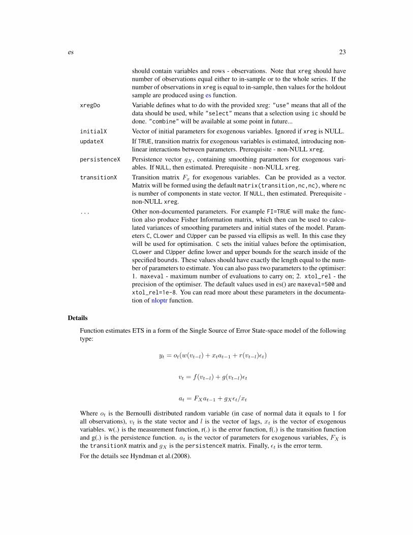
should contain variables and rows - observations. Note that xreg should havenumber of observations equal either to in-sample or to the whole series. If thenumber of observations in xreg is equal to in-sample, then values for the holdoutsample are produced using es function.


initialX Vector of initial parameters for exogenous variables. Ignored if xreg is NULL.updateX If TRUE, transition matrix for exogenous variables is estimated, introducing non-

linear interactions between parameters. Prerequisite - non-NULL xreg.persistenceX Persistence vector gX , containing smoothing parameters for exogenous vari-

ables. If NULL, then estimated. Prerequisite - non-NULL xreg.transitionX Transition matrix Fx for exogenous variables. Can be provided as a vector.

Matrix will be formed using the default matrix(transition,nc,nc), where ncis number of components in state vector. If NULL, then estimated. Prerequisite -non-NULL xreg.

... Other non-documented parameters. For example FI=TRUE will make the func-tion also produce Fisher Information matrix, which then can be used to calcu-lated variances of smoothing parameters and initial states of the model. Param-eters C, CLower and CUpper can be passed via ellipsis as well. In this case theywill be used for optimisation. C sets the initial values before the optimisation,CLower and CUpper define lower and upper bounds for the search inside of thespecified bounds. These values should have exactly the length equal to the num-ber of parameters to estimate. You can also pass two parameters to the optimiser:1. maxeval - maximum number of evaluations to carry on; 2. xtol_rel - theprecision of the optimiser. The default values used in es() are maxeval=500 andxtol_rel=1e-8. You can read more about these parameters in the documenta-tion of nloptr function.

Details

Function estimates ETS in a form of the Single Source of Error State-space model of the followingtype:

yt = ot(w(vt−l) + xtat−1 + r(vt−l)εt)

vt = f(vt−l) + g(vt−l)εt

at = FXat−1 + gXεt/xt

Where ot is the Bernoulli distributed random variable (in case of normal data it equals to 1 forall observations), vt is the state vector and l is the vector of lags, xt is the vector of exogenousvariables. w(.) is the measurement function, r(.) is the error function, f(.) is the transition functionand g(.) is the persistence function. at is the vector of parameters for exogenous variables, FX isthe transitionX matrix and gX is the persistenceX matrix. Finally, εt is the error term.

For the details see Hyndman et al.(2008).

24 es

Value

Object of class "smooth" is returned. It contains the list of the following values for classical ETSmodels:

• model - type of constructed model.

• formula - mathematical formula, describing interactions between components of es() andexogenous variables.


• states - matrix of the components of ETS.

• persistence - persistence vector. This is the place, where smoothing parameters live.

• phi - value of damping parameter.

• transition - transition matrix of the model.

• initialType - type of the initial values used.

• initial - initial values of the state vector (non-seasonal).

• initialSeason - initial values of the seasonal part of state vector.


• fitted - fitted values of ETS.

• forecast - point forecast of ETS.

• lower - lower bound of prediction interval. When intervals="none" then NA is returned.

• upper - higher bound of prediction interval. When intervals="none" then NA is returned.

• residuals - residuals of the estimated model.

• errors - trace forecast in-sample errors, returned as a matrix. In the case of trace forecaststhis is the matrix used in optimisation. In non-trace estimations it is returned just for theinformation.





• actuals - original data.

• holdout - holdout part of the original data.






es 25


• ICs - values of information criteria of the model. Includes AIC, AICc and BIC.


• cf - cost function value.

• cfType - type of cost function used in the estimation.



If combination of forecasts is produced (using model="CCC"), then a shorter list of values is re-turned:

• model,

• timeElapsed,

• initialType,

• fitted,

• forecast,

• lower,

• upper,

• residuals,

• s2 - variance of additive error of combined one-step-ahead forecasts,

• intervals,

• level,

• cumulative,

• actuals,

• holdout,

• imodel,

• ICs - combined ic,

• ICw - ic weights used in the combination,

• cfType,

• xreg,

• accuracy.

Author(s)


26 es

References







• Kolassa, S. (2011) Combining exponential smoothing forecasts using Akaike weights. Inter-national Journal of Forecasting, 27, pp 238 - 251.

• Taylor, J.W. and Bunn, D.W. (1999) A Quantile Regression Approach to Generating PredictionIntervals. Management Science, Vol 45, No 2, pp 225-237.

See Also

ets, forecast,ts, sim.es

Examples

library(Mcomp)

# See how holdout and trace parameters influence the forecastes(M3$N1245$x,model="AAdN",h=8,holdout=FALSE,cfType="MSE")## Not run: es(M3$N2568$x,model="MAM",h=18,holdout=TRUE,cfType="TMSE")

# Model selection examplees(M3$N1245$x,model="ZZN",ic="AIC",h=8,holdout=FALSE,bounds="a")

# Model selection. Compare AICc of these two models:## Not run: es(M3$N1683$x,"ZZZ",h=10,holdout=TRUE)es(M3$N1683$x,"MAdM",h=10,holdout=TRUE)## End(Not run)

# Model selection, excluding multiplicative trend## Not run: es(M3$N1245$x,model="ZXZ",h=8,holdout=TRUE)

# Combination example## Not run: es(M3$N1245$x,model="CCN",h=8,holdout=TRUE)

http://dx.doi.org/10.1007/978-3-540-71918-2

http://dx.doi.org/10.1007/978-3-540-71918-2

forecast.smooth 27

# Model selection using a specified pool of modelsourModel <- es(M3$N1587$x,model=c("ANN","AAM","AMdA"),h=18)

# Redo previous model and produce prediction intervalses(M3$N1587$x,model=ourModel,h=18,intervals="p")

# Semiparametric intervals example## Not run: es(M3$N1587$x,h=18,holdout=TRUE,intervals="sp")

# Exogenous variables in ETS example## Not run: x <- cbind(c(rep(0,25),1,rep(0,43)),c(rep(0,10),1,rep(0,58)))y <- ts(c(M3$N1457$x,M3$N1457$xx),frequency=12)es(y,h=18,holdout=TRUE,xreg=x,cfType="aTMSE",intervals="np")ourModel <- es(ts(c(M3$N1457$x,M3$N1457$xx),frequency=12),h=18,holdout=TRUE,xreg=x,updateX=TRUE)## End(Not run)

# This will be the same model as in previous line but estimated on new portion of data## Not run: es(ts(c(M3$N1457$x,M3$N1457$xx),frequency=12),model=ourModel,h=18,holdout=FALSE)

# Intermittent data examplex <- rpois(100,0.2)# Intervals-based model (Croston's method) with the best ETS for demand sizeses(x,"ZZN",intermittent="i")# Intervals-based model (TSB) on iETS(M,N,N)es(x,"MNN",intermittent="p")# Constant probability based on iETS(M,N,N)es(x,"MNN",intermittent="fixed")# Best type of intermittent model based on iETS(Z,Z,N)ourModel <- es(x,"ZZN",intermittent="auto")


forecast.smooth Forecasting time series using smooth functions

Description

This function is created in order for the package to be compatible with Rob Hyndman’s "forecast"package

Usage

## S3 method for class 'smooth'forecast(object, h = 10, intervals = c("parametric","semiparametric", "nonparametric", "none"), level = 0.95, ...)

28 forecast.smooth

Arguments

object Time series model for which forecasts are required.

h Forecast horizon

intervals Type of intervals to construct. See es for details.


... Other arguments accepted by either es, ces, ges or ssarima.

Details

This is not a compulsary function. You can simply use es, ces, ges or ssarima without forecast.smooth.But if you are really used to forecast function, then go ahead!

Value

Returns object of class "smooth.forecast", which contains:

• model - the estimated model (ES / CES / GES / SSARIMA).

• method - the name of the estimated model (ES / CES / GES / SSARIMA).

• fitted - fitted values of the model.

• actuals - actuals provided in the call of the model.

• forecast aka mean - point forecasts of the model (conditional mean).

• lower - lower bound of prediction intervals.

• upper - upper bound of prediction intervals.

• level - confidence level.

• intervals - binary variable (whether intervals were produced or not).

• residuals - the residuals of the original model.

Author(s)


References

Hyndman, R.J., Koehler, A.B., Ord, J.K., and Snyder, R.D. (2008) Forecasting with exponentialsmoothing: the state space approach, Springer-Verlag. http://www.exponentialsmoothing.net.

See Also

ets, forecast

http://www.exponentialsmoothing.net

ges 29

Examples


forecast.smooth(ourModel,h=10)forecast.smooth(ourModel,h=10,intervals=TRUE)plot(forecast.smooth(ourModel,h=10,intervals=TRUE))

ges General Exponential Smoothing

Description

Function constructs General Exponential Smoothing, estimating matrices F, w, vector g and initialparameters.

Usage

ges(data, orders = c(1, 1), lags = c(1, frequency(data)), type = c("A","M"), persistence = NULL, transition = NULL, measurement = NULL,initial = c("optimal", "backcasting"), ic = c("AICc", "AIC", "BIC"),cfType = c("MSE", "MAE", "HAM", "MSEh", "TMSE", "GTMSE", "MSCE"), h = 10,holdout = FALSE, cumulative = FALSE, intervals = c("none", "parametric","semiparametric", "nonparametric"), level = 0.95, intermittent = c("none","auto", "fixed", "interval", "probability", "sba", "logistic"),imodel = "MNN", bounds = c("admissible", "none"), silent = c("all","graph", "legend", "output", "none"), xreg = NULL, xregDo = c("use","select"), initialX = NULL, updateX = FALSE, persistenceX = NULL,transitionX = NULL, ...)

Arguments


orders Order of the model. Specified as vector of number of states with different lags.For example, orders=c(1,1) means that there are two states: one of the firstlag type, the second of the second type.

lags Defines lags for the corresponding orders. If, for example, orders=c(1,1) andlags are defined as lags=c(1,12), then the model will have two states: thefirst will have lag 1 and the second will have lag 12. The length of lags mustcorrespond to the length of orders.

type Type of model. Can either be "A" - additive - or "M" - multiplicative. The lattermeans that the GES is fitted on log-transformed data.

persistence Persistence vector g, containing smoothing parameters. If NULL, then estimated.

30 ges

transition Transition matrix F . Can be provided as a vector. Matrix will be formed usingthe default matrix(transition,nc,nc), where nc is the number of compo-nents in state vector. If NULL, then estimated.

measurement Measurement vector w. If NULL, then estimated.















ges 31










... Other non-documented parameters. For example parameter model can accept apreviously estimated GES model and use all its parameters. FI=TRUE will makethe function produce Fisher Information matrix, which then can be used to cal-culated variances of parameters of the model. You can also pass two parametersto the optimiser: 1. maxeval - maximum number of evaluations to carry on; 2.xtol_rel - the precision of the optimiser. The default values used in es() aremaxeval=5000 and xtol_rel=1e-8. You can read more about these parametersin the documentation of nloptr function.

Details

The function estimates the Single Source of Error State-space model of the following type:

yt = ot(w′vt−l + xtat−1 + εt)

32 ges

vt = Fvt−l + gεt


Where ot is the Bernoulli distributed random variable (in case of normal data equal to 1), vt isthe state vector (defined using orders) and l is the vector of lags, xt is the vector of exogenousparameters. w is the measurement vector, F is the transition matrix, g is the persistencevector, at is the vector of parameters for exogenous variables, FX is the transitionX matrix andgX is the persistenceX matrix. Finally, εt is the error term.

Value

Object of class "smooth" is returned. It contains:

• model - name of the estimated model.


• states - matrix of fuzzy components of GES, where rows correspond to time and cols tostates.


• initial - initial values of state vector (extracted from states).


• measurement - matrix w.

• transition - matrix F.

• persistence - persistence vector. This is the place, where smoothing parameters live.

• fitted - fitted values of ETS.

• forecast - point forecast of ETS.

• lower - lower bound of prediction interval. When intervals="none" then NA is returned.

• upper - higher bound of prediction interval. When intervals="none" then NA is returned.


• errors - matrix of 1 to h steps ahead errors.





• actuals - original data.

• holdout - holdout part of the original data.


ges 33










• FI - Fisher Information. Equal to NULL if FI=FALSE or when FI variable is not provided atall.


Author(s)


References

• Svetunkov I. (2017). Statistical models underlying functions of ’smooth’ package for R. Work-ing Paper of Department of Management Science, Lancaster University 2017:1, 1-52.


See Also

ets, es, ces,sim.es

Examples

# Something simple:ges(rnorm(118,100,3),orders=c(1),lags=c(1),h=18,holdout=TRUE,bounds="a",intervals="p")

# A more complicated model with seasonality## Not run: ourModel <- ges(rnorm(118,100,3),orders=c(2,1),lags=c(1,4),h=18,holdout=TRUE)

# Redo previous model on a new data and produce prediction intervals## Not run: ges(rnorm(118,100,3),model=ourModel,h=18,intervals="sp")

# Produce something crazy with optimal initials (not recommended)## Not run: ges(rnorm(118,100,3),orders=c(1,1,1),lags=c(1,3,5),h=18,holdout=TRUE,initial="o")

34 graphmaker

# Simpler model estiamted using trace forecast error cost function and its analytical analogue## Not run: ges(rnorm(118,100,3),orders=c(1),lags=c(1),h=18,holdout=TRUE,bounds="n",cfType="TMSE")ges(rnorm(118,100,3),orders=c(1),lags=c(1),h=18,holdout=TRUE,bounds="n",cfType="aTMSE")## End(Not run)

# Introduce exogenous variables## Not run: ges(rnorm(118,100,3),orders=c(1),lags=c(1),h=18,holdout=TRUE,xreg=c(1:118))

# Ask for their update## Not run: ges(rnorm(118,100,3),orders=c(1),lags=c(1),h=18,holdout=TRUE,xreg=c(1:118),updateX=TRUE)

# Do the same but now let's shrink parameters...## Not run: ges(rnorm(118,100,3),orders=c(1),lags=c(1),h=18,xreg=c(1:118),updateX=TRUE,cfType="TMSE")ourModel <- ges(rnorm(118,100,3),orders=c(1),lags=c(1),h=18,holdout=TRUE,cfType="aTMSE")## End(Not run)

# Or select the most appropriate one## Not run: ges(rnorm(118,100,3),orders=c(1),lags=c(1),h=18,holdout=TRUE,xreg=c(1:118),xregDo="s")

summary(ourModel)forecast(ourModel)plot(forecast(ourModel))## End(Not run)

graphmaker Linear graph construction function

Description

The function makes a standard linear graph using at least actuals and forecasts.

Usage

graphmaker(actuals, forecast, fitted = NULL, lower = NULL, upper = NULL,level = NULL, legend = TRUE, main = NULL, cumulative = FALSE)

Arguments

actuals The vector of actual series.

forecast The vector of forecasts. Should be ts object that start at the end of fittedvalues.

fitted The vector of fitted values.

lower The vector of lower bound values of a prediction interval. Should be ts objectthat start at the end of fitted values.

upper The vector of upper bound values of a prediction interval. Should be ts objectthat start at the end of fitted values.

level The width of the prediction interval.

hm 35

legend If TRUE, the legend is drawn.

main The title of the produced plot.

cumulative If TRUE, then the forecast is treated as cumulative and value per period is plotted.

Details

Function uses the provided data to construct a linear graph. It is strongly advised to use ts functionto define the start of each of the vectors. Otherwise the data may be plotted in a wrong way.

Value

Function does not return anything.

Author(s)

Ivan Svetunkov

See Also

ts

Examples

x <- rnorm(100,0,1)values <- es(x,model="ANN",silent=TRUE,intervals=TRUE,level=0.95)

graphmaker(x,values$forecast,values$fitted)graphmaker(x,values$forecast,values$fitted,legend=FALSE)graphmaker(x,values$forecast,values$fitted,values$lower,values$upper,level=0.95)graphmaker(x,values$forecast,values$fitted,values$lower,values$upper,level=0.95,legend=FALSE)

actuals <- c(1:10)forecast <- ts(c(11:15),start=end(actuals)[1]+end(actuals)[2]*deltat(actuals),

frequency=frequency(actuals))graphmaker(actuals,forecast)

hm Half moment of a distribution and its derivatives.

Description

hm function estimates half moment from some predefined constant C. cbias function calculates biasbased on hm.

36 iss

Usage

hm(x, C = mean(x), digits = 5, ...)

cbias(x, C = mean(x), digits = 5, ...)

Arguments

x A variable based on which HM is estimated.

C Centering parameter.

digits Number of digits for rounding.

... Other parameters passed to mean function.

Details

NA values of x are excluded on the first step of calculation.

Value

A complex variable is returned for hm function and real value is returned for cbias.

Author(s)


Examples

x <- rnorm(100,0,1)hm(x)cbias(x)

iss Intermittent State Space

Description

Function calculates the probability for intermittent state space model. This is needed in order toforecast intermittent demand using other functions.

Usage

iss(data, intermittent = c("none", "fixed", "interval", "probability", "sba","logistic"), ic = c("AICc", "AIC", "BIC"), h = 10, holdout = FALSE,model = NULL, persistence = NULL, initial = NULL,initialSeason = NULL, xreg = NULL)

iss 37

Arguments

data Either numeric vector or time series vector.

intermittent Type of method used in probability estimation. Can be "none" - none, "fixed"- constant probability, "croston" - estimated using Croston, 1972 method and"TSB" - Teunter et al., 2011 method., "sba" - Syntetos-Boylan Approximationfor Croston’s method (bias correction) discussed in Syntetos and Boylan, 2005,"logistic" - probability based on logit model.

ic Information criteria to use in case of model selection.

h Forecast horizon.


model Type of ETS model used for the estimation. Normally this should be either"ANN" or "MNN".

persistence Persistence vector. If NULL, then it is estimated.

initial Initial vector. If NULL, then it is estimated.

initialSeason Initial vector of seasonal components. If NULL, then it is estimated.

xreg Vector of matrix of exogenous variables, explaining some parts of occurrencevariable (probability).

Details

The function estimates probability of demand occurrence, using one of the ETS state-space models.

Value

The object of class "iss" is returned. It contains following list of values:

• model - the type of the estimated ETS model;

• fitted - fitted values of the constructed model;

• forecast - forecast for h observations ahead;

• states - values of states (currently level only);

• variance - conditional variance of the forecast;

• logLik - likelihood value for the model

• nParam - number of parameters used in the model;

• residuals - residuals of the model;

• actuals - actual values of probabilities (zeros and ones).

• persistence - the vector of smoothing parameters;

• initial - initial values of the state vector;

• initialSeason - the matrix of initials seasonal states;

Author(s)


38 MPE

References





See Also

ets, forecast,es

Examples

y <- rpois(100,0.1)iss(y, intermittent="p")

iss(y, intermittent="i", persistence=0.1)

MPE Error measures

Description

Functions allow to calculate different types of errors:

1. MPE - Mean Percentage Error,

2. MAPE - Mean Absolute Percentage Error,

3. SMAPE - Symmetric Mean Absolute Percentage Error,

4. MASE - Mean Absolute Scaled Error,

5. RelMAE - Average Relative Mean Absolute Error,

6. sMSE - Scaled Mean Squared Error,

7. sPIS- Scaled Periods-In-Stock,

8. sCE - Scaled Cumulative Error.

MPE 39

Usage

MPE(actual, forecast, digits = 3)

MAPE(actual, forecast, digits = 3)

SMAPE(actual, forecast, digits = 3)

MASE(actual, forecast, scale, digits = 3)

RelMAE(actual, forecast, benchmark, digits = 3)

sMSE(actual, forecast, scale, digits = 3)

sPIS(actual, forecast, scale, digits = 3)

sCE(actual, forecast, scale, digits = 3)

Arguments

actual The vector or matrix of actual values.

forecast The vector or matrix of forecasts values.

digits Number of digits of the output.

scale The value that should be used in the denominator of MASE. Can be anything butadvised values are: mean absolute deviation of in-sample one step ahead Naiveerror or mean absolute value of the in-sample actuals.

benchmark The vector or matrix of the forecasts of the benchmark model.

Details

In case of sMSE, scale needs to be a squared value. Typical one – squared mean value of in-sampleactuals.

Value

All the functions return the scalar value.

Author(s)


References

• Fildes, R. (1992). The evaluation of extrapolative forecasting methods. International Journalof Forecasting, 8, pp.81-98.

• Hyndman R.J., Koehler A.B. (2006). Another look at measures of forecast accuracy. Interna-tional Journal of Forecasting, 22, pp.679-688.

40 nParam

• Makridakis, S. (1993). Accuracy measures: Theoretical and practical concerns. InternationalJournal of Forecasting, 9, pp.527-529.

• Petropoulos F., Kourentzes N. (2015). Forecast combinations for intermittent demand. Journalof the Operational Research Society, 66, pp.914-924.

• Wallstrom P., Segerstedt A. (2010). Evaluation of forecasting error measurements and tech-niques for intermittent demand. International Journal of Production Economics, 128, pp.625-636.

Examples

y <- rnorm(100,10,2)esmodel <- es(y[1:90],model="ANN",h=10)

MPE(y[91:100],esmodel$forecast,digits=5)MAPE(y[91:100],esmodel$forecast,digits=5)SMAPE(y[91:100],esmodel$forecast,digits=5)MASE(y[91:100],esmodel$forecast,mean(abs(y[1:90])),digits=5)MASE(y[91:100],esmodel$forecast,mean(abs(diff(y[1:90]))),digits=5)

esmodel2 <- es(y[1:90],model="AAN",h=10)RelMAE(y[91:100],esmodel2$forecast,esmodel$forecast,digits=5)

MASE(y[91:100],esmodel$forecast,mean(abs(y[1:90]))^2,digits=5)

sMSE(y[91:100],esmodel$forecast,mean(abs(y[1:90])),digits=5)sPIS(y[91:100],esmodel$forecast,mean(abs(y[1:90])),digits=5)sCE(y[91:100],esmodel$forecast,mean(abs(y[1:90])),digits=5)

nParam Number of parameters in the model

Description

This function returns the number of estimated parameters in the model

Usage

nParam(object, ...)

Arguments


... Some other parameters passed to the method.

orders 41

Details

This is a very basic and a simple function which does what it says: extracts number of parametersin the estimated model.

Value

This function returns a numeric value.

Author(s)


See Also

nobs, logLik

Examples


nParam(ourModel)

orders Functions that extract values from the fitted model

Description

These functions allow extracting orders and lags for ssarima(), ges() and sma() and type ofmodel from es() and ces().

Usage

orders(object, ...)

lags(object, ...)

modelType(object, ...)

Arguments

object Model estimated using one of the functions of smooth package.

... Currently nothing is accepted via ellipsis.

42 orders

Details

orders() and lags() are useful only for SSARIMA, GES and SMA. They return NA for otherfunctions. This can also be applied to arima(), Arima() and auto.arima() functions from statsand forecast packages. modelType() is useful only for ETS and CES. They return NA for otherfunctions. This can also be applied to ets() function from forecast package.

Value

Either vector or list with values is returned. orders() in case of ssarima returns list of values:

• ar - AR orders.

• i - I orders.

• ma - MA orders.

Author(s)


See Also

forecast, ssarima

Examples

x <- rnorm(100,0,1)

# Just as example. orders and lags do not return anything for ces() and es(). But modelType() does.ourModel <- ces(x, h=10)orders(ourModel)lags(ourModel)modelType(ourModel)# And as another example it does the opposite for ges() and ssarima()ourModel <- ges(x, h=10, orders=c(1,1), lags=c(1,4))orders(ourModel)lags(ourModel)modelType(ourModel)

# Finally these values can be used for simulate functions or original functions.ourModel <- auto.ssarima(x)ssarima(x, orders=orders(ourModel), lags=lags(ourModel), constant=ourModel$constant)sim.ssarima(orders=orders(ourModel), lags=lags(ourModel), constant=ourModel$constant)

pls 43

pls Prediction Likelihood Score

Description

Function estimates Prediction Likelihood Score of the holdout actuals based on the model.

Usage

pls(actuals, forecasts, Etype = c("A", "M"), sigma, trace = TRUE,iprob = 1, digits = 5, varVec = NULL, rounded = FALSE, ...)

Arguments

actuals Actual values from the holdout.

forecasts Point forecasts for the holdout (conditional mean).

Etype Type of the error. If Etype="A", then normal distribution is used, if Etype="M",then log-normal distribution is used.

sigma Value of variance of the errors. In case of trace=TRUE, this needs to be a co-variance matrix of trace errors.

trace If TRUE, then it is assumed that we are provided with trace forecasts (multiplesteps ahead), Trace Forecast Likelihood is used in this case.

iprob Vector of probabilities of occurrences for the holdout (only needed for intermit-tent models).

digits Number of digits for rounding.

varVec Vector of 1 to h steps ahead analytical variance. Needed mainly for Etype=="M".

rounded Defines if the rounded up value is used for demand sizes.

... Other parameters passed to mean function.

Details

Prediction likelihood score (PLS) is based on either normal or log-normal distribution of errorswith the provided parameters. It returns the log of probability that the data was "produced" by theestimated model.

Value

A value of the log-likelihood.

Author(s)


44 pointLik

References

• Snyder, R. D., Ord, J. K., Beaumont, A., 2012. Forecasting the intermittent demand forslow-moving inventories: A modelling approach. International Journal of Forecasting 28 (2),485-496.

• Kolassa, S., 2016. Evaluating predictive count data distributions in retail sales forecasting.International Journal of Forecasting 32 (3), 788-803.

Examples

# pls() function now works correctly only when varVec is provided# And varVec is not provided by any function, but is generated inside them.

# Generate data, apply es() with the holdout parameter and calculate PLSx <- rnorm(100,0,1)ourModel <- es(x, h=10, holdout=TRUE, intervals=TRUE)sigma <- t(ourModel$errors) %*% (ourModel$errors) / length(ourModel$residuals)Etype <- substr(modelType(ourModel),1,1)pls(actuals=ourModel$holdout, forecasts=ourModel$forecast, Etype=Etype,

sigma=sigma, trace=TRUE)

# Do the same with intermittent data. Trace is not available yet for# intermittent state-space modelsx <- rpois(100,0.4)ourModel <- es(x, h=10, holdout=TRUE, intermittent='a', intervals=TRUE)Etype <- substr(modelType(ourModel),1,1)iprob <- ourModel$imodel$fittedpls(actuals=ourModel$holdout, forecasts=ourModel$forecast, Etype=Etype,

sigma=ourModel$s2, trace=FALSE, iprob=iprob)

pointLik Point likelihood values

Description

This function returns a vector of logarithms of likelihoods for each observation

Usage

pointLik(object, ...)

Arguments


... Some stuff.

sim.ces 45

Details

Instead of taking the expected log-likelihood for the whole series, this function calculates the indi-vidual value for each separate observation. Note that these values are biased, so you would possiblyneed to take number of degrees of freedom into account in order to have an unbiased estimator.

Value

This function returns a vector.

Author(s)


See Also

AIC, BIC

Examples


pointLik(ourModel)

# Bias correctionpointLik(ourModel) - nParam(ourModel)

# Bias correction in AIC style2*(nParam(ourModel) - pointLik(ourModel))

# BIC calculation based on pointLiklog(nobs(ourModel))*nParam(ourModel) - 2*sum(pointLik(ourModel))

sim.ces Simulate Complex Exponential Smoothing

Description

Function generates data using CES with Single Source of Error as a data generating process.

Usage

sim.ces(seasonality = c("none", "simple", "partial", "full"), obs = 10,nsim = 1, frequency = 1, A = NULL, B = NULL, initial = NULL,randomizer = c("rnorm", "runif", "rbeta", "rt"), iprob = 1, ...)

46 sim.ces

Arguments

seasonality The type of seasonality used in CES. Can be: none - No seasonality; simple -Simple seasonality, using lagged CES (based on t-m observation, where m is theseasonality lag); partial - Partial seasonality with real seasonal components(equivalent to additive seasonality); full - Full seasonality with complex sea-sonal components (can do both multiplicative and additive seasonality, depend-ing on the data). First letter can be used instead of full words. Any seasonalCES can only be constructed for time series vectors.

obs Number of observations in each generated time series.

nsim Number of series to generate (number of simulations to do).

frequency Frequency of generated data. In cases of seasonal models must be greater than1.

A First complex smoothing parameter. Should be a complex number.NOTE! CES is very sensitive to A and B values so it is advised to use valuesfrom previously estimated model.

B Second complex smoothing parameter. Can be real if seasonality="partial".In case of seasonality="full" must be complex number.

initial A matrix with initial values for CES. In case with seasonality="partial"and seasonality="full" first two columns should contain initial values fornon-seasonal components, repeated frequency times.

randomizer Type of random number generator function used for error term. Defaults are:rnorm, rt, runif, rbeta. But any function from Distributions will do the trickif the appropriate parameters are passed. For example rpois with lambda=2 canbe used as well.

iprob Probability of occurrence, used for intermittent data generation. This can be avector, implying that probability varies in time (in TSB or Croston style).

... Additional parameters passed to the chosen randomizer. All the parametersshould be passed in the order they are used in chosen randomizer. For example,passing just sd=0.5 to rnorm function will lead to the call rnorm(obs, mean=0.5, sd=1).

Value

List of the following values is returned:

• model - Name of CES model.

• A - Value of complex smoothing parameter A. If nsim>1, then this is a vector.

• B - Value of complex smoothing parameter B. If seasonality="n" or seasonality="s",then this is equal to NULL. If nsim>1, then this is a vector.

• initial - Initial values of CES in a form of matrix. If nsim>1, then this is an array.

• data - Time series vector (or matrix if nsim>1) of the generated series.

• states - Matrix (or array if nsim>1) of states. States are in columns, time is in rows.

• residuals - Error terms used in the simulation. Either vector or matrix, depending on nsim.

• occurrences - Values of occurrence variable. Once again, can be either a vector or a matrix...

• logLik - Log-likelihood of the constructed model.

sim.es 47

Author(s)


References



See Also

sim.es, sim.ssarima,ces, Distributions

Examples

# Create 120 observations from CES(n). Generate 100 time series of this kind.x <- sim.ces("n",obs=120,nsim=100)

# Generate similar thing for seasonal series of CES(s)_4x <- sim.ces("s",frequency=4,obs=80,nsim=100)

# Estimate model and then generate 10 time series from itourModel <- ces(rnorm(100,100,5))simulate(ourModel,nsim=10)

sim.es Simulate Exponential Smoothing

Description

Function generates data using ETS with Single Source of Error as a data generating process.

Usage

sim.es(model = "ANN", obs = 10, nsim = 1, frequency = 1,persistence = NULL, phi = 1, initial = NULL, initialSeason = NULL,bounds = c("usual", "admissible", "restricted"), randomizer = c("rnorm","rlnorm", "runif", "rbeta", "rt"), iprob = 1, ...)

48 sim.es

Arguments

model Type of ETS model according to [Hyndman et. al., 2008] taxonomy. Can consistof 3 or 4 chars: ANN, AAN, AAdN, AAA, AAdA, MAdM etc.




persistence Persistence vector, which includes all the smoothing parameters. Must corre-spond to the chosen model. The maximum length is 3: level, trend and seasonalsmoothing parameters. If NULL, values are generated.

phi Value of damping parameter. If trend is not chosen in the model, the parameteris ignored.

initial Vector of initial states of level and trend. The maximum length is 2. If NULL,values are generated.

initialSeason Vector of initial states for seasonal coefficients. Should have length equal tofrequency parameter. If NULL, values are generated.

bounds Type of bounds to use for persistence vector if values are generated. "usual"- bounds from p.156 by Hyndman et. al., 2008. "restricted" - similar to"usual" but with upper bound equal to 0.3. "admissible" - bounds from tables10.1 and 10.2 of Hyndman et. al., 2008. Using first letter of the type of boundsalso works. These bounds are also used for multiplicative models, so be careful!



... Additional parameters passed to the chosen randomizer. All the parametersshould be passed in the order they are used in chosen randomizer. For example,passing just sd=0.5 to rnorm function will lead to the call rnorm(obs, mean=0.5, sd=1).ATTENTION! When generating the multiplicative errors some tuning might beneeded to obtain meaningful data. sd=0.1 is usually already a high value forsuch models.

Value


• model - Name of ETS model.



• persistence - Vector (or matrix if nsim>1) of smoothing parameters used in the simulation.

• phi - Value of damping parameter used in time series generation.

• initial - Vector (or matrix) of initial values.

sim.es 49

• initialSeason - Vector (or matrix) of initial seasonal coefficients.

• iprob - vector of probabilities used in the simulation.

• intermittent - type of the intermittent model used.




Author(s)


References



See Also

es, ets,forecast, ts, Distributions

Examples

# Create 40 observations of quarterly data using AAA model with errors from normal distributionETS.AAA <- sim.es(model="AAA",frequency=4,obs=40,randomizer="rnorm",mean=0,sd=100)

# Create 50 series of quarterly data using AAA model# with 40 observations each with errors from normal distributionETS.AAA <- sim.es(model="AAA",frequency=4,obs=40,randomizer="rnorm",mean=0,sd=100,nsim=50)

# Create 50 series of quarterly data using AAdA model# with 40 observations each with errors from normal distribution# and smoothing parameters lying in the "admissible" range.ETS.AAA <- sim.es(model="AAA",phi=0.9,frequency=4,obs=40,bounds="admissible",

randomizer="rnorm",mean=0,sd=100,nsim=50)

# Create 60 observations of monthly data using ANN model# with errors from beta distributionETS.ANN <- sim.es(model="ANN",persistence=c(1.5),frequency=12,obs=60,

randomizer="rbeta",sshape1=1.5,sshape2=1.5)plot(ETS.ANN$states)

# Create 60 observations of monthly data using MAM model# with errors from uniform distributionETS.MAM <- sim.es(model="MAM",persistence=c(0.3,0.2,0.1),initial=c(2000,50),

phi=0.8,frequency=12,obs=60,randomizer="runif",min=-0.5,max=0.5)

http://dx.doi.org/10.1007/978-3-540-71918-2

http://dx.doi.org/10.1007/978-3-540-71918-2

50 sim.ges

# Create 80 observations of quarterly data using MMM model# with predefined initial values and errors from the normal distributionETS.MMM <- sim.es(model="MMM",persistence=c(0.1,0.1,0.1),initial=c(2000,1),

initialSeason=c(1.1,1.05,0.9,.95),frequency=4,obs=80,mean=0,sd=0.01)

# Generate intermittent data using AAdNiETS.AAdN <- sim.es("AAdN",frequency=1,obs=30,iprob=0.1,initial=c(3,0),phi=0.8)

# Generate iETS(MNN) with TSB style probabilitiespt <- sim.es("MNN",persistence=0.2,initial=0.5,obs=50,mean=0,sd=0.3)iprob <- mean(rbeta(50,shape1=pt$states,shape2=1-pt$states))iETS.MNN <- sim.es("MNN",frequency=12,persistence=0.2,initial=4,iprob=iprob,obs=50)

sim.ges Simulate Generalised Exponential Smoothing

Description

Function generates data using GES with Single Source of Error as a data generating process.

Usage

sim.ges(orders = c(1), lags = c(1), obs = 10, nsim = 1, frequency = 1,measurement = NULL, transition = NULL, persistence = NULL,initial = NULL, randomizer = c("rnorm", "runif", "rbeta", "rt"),iprob = 1, ...)

Arguments

orders Order of the model. Specified as vector of number of states with different lags.For example, orders=c(1,1) means that there are two states: one of the firstlag type, the second of the second type.

lags Defines lags for the corresponding orders. If, for example, orders=c(1,1) andlags are defined as lags=c(1,12), then the model will have two states: thefirst will have lag 1 and the second will have lag 12. The length of lags mustcorrespond to the length of orders.




measurement Measurement vector w. If NULL, then estimated.

transition Transition matrix F . Can be provided as a vector. Matrix will be formed usingthe default matrix(transition,nc,nc), where nc is the number of compo-nents in state vector. If NULL, then estimated.

persistence Persistence vector g, containing smoothing parameters. If NULL, then estimated.

sim.ges 51

initial Vector of initial values for state matrix. If NULL, then generated using advanced,sophisticated technique - uniform distribution.




Value


• model - Name of GES model.

• measurement - Matrix w.

• transition - Matrix F.

• persistence - Persistence vector. This is the place, where smoothing parameters live.

• initial - Initial values of GES in a form of matrix. If nsim>1, then this is an array.






Author(s)


References


See Also

sim.es, sim.ssarima,sim.ces, ges, Distributions

52 sim.sma

Examples

# Create 120 observations from GES(1[1]). Generate 100 time series of this kind.x <- sim.ges(orders=c(1),lags=c(1),obs=120,nsim=100)

# Generate similar thing for seasonal series of GES(1[1],1[4]])x <- sim.ges(orders=c(1,1),lags=c(1,4),frequency=4,obs=80,nsim=100,transition=c(1,0,0.9,0.9))

# Estimate model and then generate 10 time series from itourModel <- ges(rnorm(100,100,5))simulate(ourModel,nsim=10)

sim.sma Simulate Simple Moving Average

Description

Function generates data using SMA in a Single Source of Error state-space model as a data gener-ating process.

Usage

sim.sma(order = NULL, obs = 10, nsim = 1, frequency = 1,initial = NULL, randomizer = c("rnorm", "rlnorm", "runif", "rbeta", "rt"),iprob = 1, ...)

Arguments

order Order of the modelled series. If omitted, then a random order from 1 to 100 isselected.




initial Vector of initial states for the model. If NULL, values are generated.




sim.sma 53

Value


• model - Name of SMA model.



• initial - Vector (or matrix) of initial values.

• iprob - vector of probabilities used in the simulation.

• intermittent - type of the intermittent model used.




Author(s)


References



See Also

es, ets,forecast, ts, Distributions

Examples

# Create 40 observations of quarterly data using AAA model with errors from normal distributionsma10 <- sim.sma(order=10,frequency=4,obs=40,randomizer="rnorm",mean=0,sd=100)

http://dx.doi.org/10.1007/978-3-540-71918-2

http://dx.doi.org/10.1007/978-3-540-71918-2

54 sim.ssarima

sim.ssarima Simulate SSARIMA

Description

Function generates data using SSARIMA with Single Source of Error as a data generating process.

Usage

sim.ssarima(orders = list(ar = 0, i = 1, ma = 1), lags = 1, obs = 10,nsim = 1, frequency = 1, AR = NULL, MA = NULL, constant = FALSE,initial = NULL, bounds = c("admissible", "none"),randomizer = c("rnorm", "runif", "rbeta", "rt"), iprob = 1, ...)

Arguments

orders List of orders, containing vector variables ar, i and ma. Example: orders=list(ar=c(1,2),i=c(1),ma=c(1,1,1)).If a variable is not provided in the list, then it is assumed to be equal to zero. Atleast one variable should have the same length as lags.

lags Defines lags for the corresponding orders (see examples above). The lengthof lags must correspond to the length of either ar.orders or i.orders orma.orders. There is no restrictions on the length of lags vector. It is recom-mended to order lags ascending.




AR Vector or matrix of AR parameters. The order of parameters should be lag-wise.This means that first all the AR parameters of the firs lag should be passed, thenfor the second etc. AR of another ssarima can be passed here.

MA Vector or matrix of MA parameters. The order of parameters should be lag-wise.This means that first all the MA parameters of the firs lag should be passed, thenfor the second etc. MA of another ssarima can be passed here.

constant If TRUE, constant term is included in the model. Can also be a number (constantvalue).

initial Vector of initial values for state matrix. If NULL, then generated using advanced,sophisticated technique - uniform distribution.

bounds Type of bounds to use for AR and MA if values are generated. "admissible" -bounds guaranteeing stability and stationarity of SSARIMA. "none" - we gen-erate something, but do not guarantee stationarity and stability. Using first letterof the type of bounds also works.


sim.ssarima 55


... Additional parameters passed to the chosen randomizer. All the parametersshould be passed in the order they are used in chosen randomizer. For example,passing just sd=0.5 to rnorm function will lead to the call rnorm(obs, mean=0.5, sd=1).A list of orders can be passed here using orders parameter instead of ar.orders,i.orders and ma.orders. This should be handy when using extraction functionorders(). See vignettes on simulate functions for examples.

Value


• model - Name of SSARIMA model.

• AR - Value of AR parameters. If nsim>1, then this is a matrix.

• MA - Value of MA parameters. If nsim>1, then this is a matrix.

• constant - Value of constant term. If nsim>1, then this is a vector.

• initial - Initial values of SSARIM. If nsim>1, then this is a matrix.






Author(s)


References



See Also

sim.es, ssarima,Distributions, orders, lags

Examples

# Create 120 observations from ARIMA(1,1,1) with drift. Generate 100 time series of this kind.x <- sim.ssarima(ar.orders=1,i.orders=1,ma.orders=1,obs=120,nsim=100,constant=TRUE)

# Generate similar thing for seasonal series of SARIMA(1,1,1)(0,0,2)_4

http://dx.doi.org/10.1007/978-3-540-71918-2

http://dx.doi.org/10.1007/978-3-540-71918-2

56 sma

x <- sim.ssarima(ar.orders=c(1,0),i.orders=c(1,0),ma.orders=c(1,2),lags=c(1,4),frequency=4,obs=80,nsim=100,constant=FALSE)

# Generate 10 series of high frequency data from SARIMA(1,0,2)_1(0,1,1)_7(1,0,1)_30x <- sim.ssarima(ar.orders=c(1,0,1),i.orders=c(0,1,0),ma.orders=c(2,1,1),lags=c(1,7,30),

obs=360,nsim=10)

sma Simple Moving Average

Description

Function constructs State-Space simple moving average of predefined order

Usage

sma(data, order = NULL, ic = c("AICc", "AIC", "BIC"), h = 10,holdout = FALSE, cumulative = FALSE, intervals = c("none", "parametric","semiparametric", "nonparametric"), level = 0.95, silent = c("all","graph", "legend", "output", "none"), ...)

Arguments


order Order of simple moving average. If NULL, then it is selected automatically usinginformation criteria.










sma 57




... Other non-documented parameters. For example parameter model can accept apreviously estimated SMA model and use its parameters.

Details

The function constructs AR model in the Single Source of Error State-space form based on the ideathat:

yt =1n

∑nj=1 yt−j

which is AR(n) process, that can be modelled using:

yt = w′vt−1 + εt

vt = Fvt−1 + gεt

Where vt is a state vector.

Value


• model - the name of the estimated model.


• states - the matrix of the fuzzy components of ssarima, where rows correspond to time andcols to states.


• persistence - the persistence vector. This is the place, where smoothing parameters live.

• order - order of moving average.

• initial - Initial state vector values.

• initialType - Type of initial values used.


• fitted - the fitted values of ETS.

• forecast - the point forecast of ETS.

• lower - the lower bound of prediction interval. When intervals=FALSE then NA is returned.

58 sma

• upper - the higher bound of prediction interval. When intervals=FALSE then NA is returned.







• actuals - the original data.






• accuracy - vector of accuracy measures for the holdout sample. Includes: MPE, MAPE,SMAPE, MASE, sMAE, RelMAE, sMSE and Bias coefficient (based on complex numbers).This is available only when holdout=TRUE.

Author(s)


References


See Also

ma, es,ssarima

Examples

# SMA of specific orderourModel <- sma(rnorm(118,100,3),order=12,h=18,holdout=TRUE,intervals="p")

# SMA of arbitrary orderourModel <- sma(rnorm(118,100,3),h=18,holdout=TRUE,intervals="sp")


smooth 59

smooth Smooth package

Description

Package contains functions implementing Single Source of Error state-space models for purposesof time series analysis and forecasting.

Details

Package: smoothType: PackageDate: 2016-01-27 - InfLicense: GPL-2

The following functions are included in the package:

• es - Exponential Smoothing in Single Source of Errors State Space form.

• ces - Complex Exponential Smoothing.

• ges - Generalised Exponential Smoothing.

• ssarima - SARIMA in state-space framework.

• auto.ces - Automatic selection between seasonal and non-seasonal CES.

• auto.ssarima - Automatic selection of ARIMA orders.

• sma - Simple Moving Average in state-space form.

• ves - Vector Exponential Smoothing.

• sim.es - simulate time series using ETS as a model.

• sim.ces - simulate time series using CES as a model.

• sim.ssarima - simulate time series using SARIMA as a model.

• sim.ges - simulate time series using GES as a model.

• iss - intermittent data state-space model. This function models the part with data occurrencesusing one of three methods.

There are also several methods implemented in the package for the classes "smooth" and "smooth.sim":

• orders - extracts orders of the fitted model.

• lags - extracts lags of the fitted model.

• modelType - extracts type of the fitted model.

• AICc - extracts AICc of the fitted model.

• forecast - produces forecast using provided model.

• fitted - extracts fitted values from provided model.

60 smooth

• getResponse - returns actual values from the provided model.

• residuals - extracts residuals of provided model.

• plot - plots either states of the model or produced forecast (depending on what object ispassed).

• simulate - uses sim functions in order to simulate data using the provided object.

• summary - provides summary of the object.

Author(s)

Ivan Svetunkov

Maintainer: Ivan Svetunkov <[email protected]>

References










• Kolassa, S. (2011) Combining exponential smoothing forecasts using Akaike weights. Inter-national Journal of Forecasting, 27, pp 238 - 251.


See Also

forecast, es,ssarima, ces, ges

http://dx.doi.org/10.1007/978-3-540-71918-2

http://dx.doi.org/10.1007/978-3-540-71918-2

sowhat 61

Examples

## Not run: y <- ts(rnorm(100,10,3),frequency=12)

es(y,h=20,holdout=TRUE)ges(y,h=20,holdout=TRUE)auto.ces(y,h=20,holdout=TRUE)auto.ssarima(y,h=20,holdout=TRUE)## End(Not run)

sowhat Function returns the ultimate answer to any question

Description

You need description? So what?

Usage

sowhat(...)

Arguments

... Any number of variables or string with a question.

Details

You need details? So what?

Value

It doesn’t return any value, only messages. So what?

Author(s)

Ivan Svetunkov

References

• Sowhat?

• Sowhat?

• 42

See Also

Nowwhat (to be implemented),

http://en.wiktionary.org/wiki/so_what

https://www.youtube.com/watch?v=FJfFZqTlWrQ

http://en.wikipedia.org/wiki/Douglas_Adams

62 ssarima

Examples

x <- rnorm(10000,0,1);sowhat(x);

sowhat("What's the meaning of life?")

sowhat("I don't have a girlfriend.")

ssarima State-Space ARIMA

Description

Function constructs State-Space ARIMA, estimating AR, MA terms and initial states.

Usage

ssarima(data, orders = list(ar = c(0), i = c(1), ma = c(1)), lags = c(1),constant = FALSE, AR = NULL, MA = NULL, initial = c("backcasting","optimal"), ic = c("AICc", "AIC", "BIC"), cfType = c("MSE", "MAE", "HAM","MSEh", "TMSE", "GTMSE", "MSCE"), h = 10, holdout = FALSE,cumulative = FALSE, intervals = c("none", "parametric", "semiparametric","nonparametric"), level = 0.95, intermittent = c("none", "auto", "fixed","interval", "probability", "sba", "logistic"), imodel = "MNN",bounds = c("admissible", "none"), silent = c("all", "graph", "legend","output", "none"), xreg = NULL, xregDo = c("use", "select"),initialX = NULL, updateX = FALSE, persistenceX = NULL,transitionX = NULL, ...)

Arguments


orders List of orders, containing vector variables ar, i and ma. Example: orders=list(ar=c(1,2),i=c(1),ma=c(1,1,1)).If a variable is not provided in the list, then it is assumed to be equal to zero. Atleast one variable should have the same length as lags.

lags Defines lags for the corresponding orders (see examples above). The length oflags must correspond to the length of either ar, i or ma in orders variable.There is no restrictions on the length of lags vector. It is recommended to orderlags ascending.

constant If TRUE, constant term is included in the model. Can also be a number (constantvalue).

AR Vector or matrix of AR parameters. The order of parameters should be lag-wise.This means that first all the AR parameters of the firs lag should be passed, thenfor the second etc. AR of another ssarima can be passed here.

ssarima 63

MA Vector or matrix of MA parameters. The order of parameters should be lag-wise.This means that first all the MA parameters of the firs lag should be passed, thenfor the second etc. MA of another ssarima can be passed here.















64 ssarima










... Other non-documented parameters.Vectors of orders can be passed here using ar.orders, i.orders and ma.orders.orders variable needs to be NULL in this case.Parameter model can accept a previously estimated SSARIMA model and useall its parameters.FI=TRUE will make the function produce Fisher Information matrix, which thencan be used to calculated variances of parameters of the model.

Details

The basic ARIMA(p,d,q) used in the function has the following form:

(1−B)d(1− a1B − a2B2 − ...− apB

p)y[t] = (1 + b1B + b2B2 + ...+ bqB

q)ε[t] + c

where y[t] is the actual values, ε[t] is the error term, ai, bj are the parameters for AR and MArespectively and c is the constant. In case of non-zero differences c acts as drift.

ssarima 65

This model is then transformed into ARIMA in the Single Source of Error State-space form (pro-posed in Snyder, 1985):

yt = ot(w′vt−l + xtat−1 + εt)

vt = Fvt−l + gεt


Where ot is the Bernoulli distributed random variable (in case of normal data equal to 1), vt is thestate vector (defined based on orders) and l is the vector of lags, xt is the vector of exogenousparameters. w is the measurement vector, F is the transition matrix, g is the persistencevector, at is the vector of parameters for exogenous variables, FX is the transitionX matrix andgX is the persistenceX matrix.

Due to the flexibility of the model, multiple seasonalities can be used. For example, somethingcrazy like this can be constructed: SARIMA(1,1,1)(0,1,1)[24](2,0,1)[24*7](0,0,1)[24*30], but theestimation may take some finite time...

Value


• model - the name of the estimated model.


• states - the matrix of the fuzzy components of ssarima, where rows correspond to time andcols to states.


• persistence - the persistence vector. This is the place, where smoothing parameters live.

• AR - the matrix of coefficients of AR terms.

• I - the matrix of coefficients of I terms.

• MA - the matrix of coefficients of MA terms.

• constant - the value of the constant term.


• initial - the initial values of the state vector (extracted from states).


• fitted - the fitted values of ETS.

• forecast - the point forecast of ETS.

• lower - the lower bound of prediction interval. When intervals="none" then NA is returned.

• upper - the higher bound of prediction interval. When intervals="none" then NA is re-turned.




66 ssarima




• actuals - the original data.














Author(s)


References




See Also

auto.arima, orders,lags, sim.ssarima

http://dx.doi.org/10.1007/978-3-540-71918-2

http://dx.doi.org/10.1007/978-3-540-71918-2

ssarima 67

Examples

# ARIMA(1,1,1) fitted to some dataourModel <- ssarima(rnorm(118,100,3),orders=list(ar=c(1),i=c(1),ma=c(1)),lags=c(1),h=18,

holdout=TRUE,intervals="p")

# The previous one is equivalent to:## Not run: ourModel <- ssarima(rnorm(118,100,3),ar.orders=c(1),i.orders=c(1),ma.orders=c(1),lags=c(1),h=18,

holdout=TRUE,intervals="p")## End(Not run)

# Model with the same lags and orders, applied to a different datassarima(rnorm(118,100,3),orders=orders(ourModel),lags=lags(ourModel),h=18,holdout=TRUE)

# The same model applied to a different datassarima(rnorm(118,100,3),model=ourModel,h=18,holdout=TRUE)

# Example of SARIMA(2,0,0)(1,0,0)[4]## Not run: ssarima(rnorm(118,100,3),orders=list(ar=c(2,1)),lags=c(1,4),h=18,holdout=TRUE)

# SARIMA(1,1,1)(0,0,1)[4] with different initialisations## Not run: ssarima(rnorm(118,100,3),orders=list(ar=c(1),i=c(1),ma=c(1,1)),

lags=c(1,4),h=18,holdout=TRUE)ssarima(rnorm(118,100,3),orders=list(ar=c(1),i=c(1),ma=c(1,1)),

lags=c(1,4),h=18,holdout=TRUE,initial="o")## End(Not run)

# SARIMA of a perculiar order on AirPassengers data## Not run: ssarima(AirPassengers,orders=list(ar=c(1,0,3),i=c(1,0,1),ma=c(0,1,2)),lags=c(1,6,12),

h=10,holdout=TRUE)## End(Not run)

# ARIMA(1,1,1) with Mean Squared Trace Forecast Error## Not run: ssarima(rnorm(118,100,3),orders=list(ar=1,i=1,ma=1),lags=1,h=18,holdout=TRUE,cfType="TMSE")ssarima(rnorm(118,100,3),orders=list(ar=1,i=1,ma=1),lags=1,h=18,holdout=TRUE,cfType="aTMSE")## End(Not run)

# SARIMA(0,1,1) with exogenous variablesssarima(rnorm(118,100,3),orders=list(i=1,ma=1),h=18,holdout=TRUE,xreg=c(1:118))

# SARIMA(0,1,1) with exogenous variables with crazy estimation of xreg## Not run: ourModel <- ssarima(rnorm(118,100,3),orders=list(i=1,ma=1),h=18,holdout=TRUE,

xreg=c(1:118),updateX=TRUE)## End(Not run)


68 stepwise

stepwise Stepwise selection of regressors

Description

Function selects variables that give linear regression with the lowest information criteria. The se-lection is done stepwise (forward) based on partial correlations. This should be a simpler and fasterimplementation than step() function from ‘stats’ package.

Usage

stepwise(data, ic = c("AICc", "AIC", "BIC"), silent = TRUE, df = NULL)

Arguments

data Data frame containing dependant variable in the first column and the others inthe rest.

ic Information criterion to use.silent If silent=FALSE, then nothing is silent, everything is printed out. silent=TRUE

means that nothing is produced.df Number of degrees of freedom to add (should be used if stepwise is used on

residuals).

Details

The algorithm uses lm() to fit different models and cor() to select the next regressor in the sequence.

Value

Function returns model - the final model of the class "lm".

Author(s)


See Also

step, xregExpander

Examples

xreg <- cbind(rnorm(100,10,3),rnorm(100,50,5))xreg <- cbind(100+0.5*xreg[,1]-0.75*xreg[,2]+rnorm(100,0,3),xreg,rnorm(100,300,10))colnames(xreg) <- c("y","x1","x2","Noise")

stepwise(xreg)

ves 69

ves Vector Exponential Smoothing in SSOE state-space model

Description

Function constructs vector ETS model and returns forecast, fitted values, errors and matrix of statesalong with other useful variables.

Usage

ves(data, model = "ANN", persistence = c("group", "independent","dependent"), transition = c("group", "independent", "dependent"),phi = c("group", "individual"), initial = c("individual", "group"),initialSeason = c("group", "individual"), cfType = c("likelihood","diagonal", "trace"), ic = c("AICc", "AIC", "BIC"), h = 10,holdout = FALSE, intervals = c("none", "conditional", "unconditional","independent"), level = 0.95, cumulative = FALSE,intermittent = c("none", "fixed", "logistic"), imodel = "ANN",iprobability = c("dependent", "independent"), bounds = c("admissible","none"), silent = c("all", "graph", "output", "none"), ...)

Arguments

data The matrix with data, where series are in columns and observations are in rows.

model The type of ETS model. Can consist of 3 or 4 chars: ANN, AAN, AAdN, AAA,AAdA, MMdM etc. ZZZ means that the model will be selected based on the cho-sen information criteria type. ATTENTION! ONLY PURE ADDITIVE ANDPURE MULTIPLICATIVE MODELS ARE CURRENTLY AVAILABLE + NOMODEL SELECTION IS AVAILABLE AT THIS STAGE! Pure multiplicativemodels are done as additive model applied to log(data).Also model can accept a previously estimated VES model and use all its param-eters.Keep in mind that model selection with "Z" components uses Branch and Boundalgorithm and may skip some models that could have slightly smaller informa-tion criteria.

persistence Persistence matrix G, containing smoothing parameters. Can be:

• independent - each series has its own smoothing parameters and no inter-actions are modelled (all the other values in the matrix are set to zero);

• dependent - each series has its own smoothing parameters, but interactionsbetween the series are modelled (the whole matrix is estimated);

• group each series has the same smoothing parameters for respective com-ponents (the values of smoothing parameters are repeated, all the other val-ues in the matrix are set to zero).

• provided by user as a vector or as a matrix. The value is used by the model.

transition Transition matrix F . Can be:

70 ves

• independent - each series has its own preset transition matrix and no in-teractions are modelled (all the other values in the matrix are set to zero);

• dependent - each series has its own transition matrix, but interactions be-tween the series are modelled (the whole matrix is estimated). The esti-mated model behaves similar to VAR in this case;

• group each series has the same transition matrix for respective components(the values are repeated, all the other values in the matrix are set to zero).

• provided by user as a vector or as a matrix. The value is used by the model.

phi In cases of damped trend this parameter defines whether the phi should be esti-mated separately for each series (individual) or for the whole set (group). Ifvector or a value is provided here, then it is used by the model.

initial Can be either character or a vector / matrix of initial states. If it is character,then it can be "individual", individual values of the initial non-seasonal com-ponents are used, or "group", meaning that the initials for all the time series areset to be equal to the same value. If vector of states is provided, then it is auto-matically transformed into a matrix, assuming that these values are provided forthe whole group.

initialSeason Can be either character or a vector / matrix of initial states. Treated the sameway as initial. This means that different time series may share the same initialseasonal component.

cfType Type of Cost Function used in optimization. cfType can be:

• likelihood - which assumes the minimisation of the determinant of thecovariance matrix of errors between the series. This implies that the seriescould be correlated;

• diagonal - the covariance matrix is assumed to be diagonal with zeros offthe diagonal. The determinant of this matrix is just a product of variances.This thing is minimised in this situation in logs.

• trace - the trace of the covariance matrix. The sum of variances is min-imised in this case.




intervals Type of intervals to construct. NOT AVAILABLE YET!This can be:

• none, aka n - do not produce prediction intervals.• conditional, c - produces multidimensional elliptic intervals for each step

ahead forecast.• unconditional, u - produces separate bounds for each series based on

ellipses for each step ahead. These bounds correspond to min and maxvalues of the ellipse assuming that all the other series but one take valuesin the centre of the ellipse. This leads to less accurate estimates of bounds(wider intervals than needed), but these could still be useful.

• independent, i - produces intervals based on variances of each separateseries. This does not take vector structure into account.

ves 71

The parameter also accepts TRUE and FALSE. The former means that conditionalintervals are constructed, while the latter is equivalent to none.



intermittent Defines type of intermittent model used. Can be:

• none, meaning that the data should be considered as non-intermittent;• fixed, taking into account constant Bernoulli distribution of demand oc-

currences;• tsb, based on Teunter et al., 2011 method.• auto - automatic selection of intermittency type based on information cri-

teria. The first letter can be used instead.

imodel Either character specifying what type of VES / ETS model should be used forprobability modelling, or a model estimated using viss function.

iprobability Type of multivariate probability used in the model. Can be either "independent"or "dependent". In the former case it is assumed that non-zeroes occur in eachseries independently. In the latter case each possible outcome is treated sepa-rately.

bounds What type of bounds to use in the model estimation. The first letter can be usedinstead of the whole word. Currently only "admissible" bounds are available.


... Other non-documented parameters. For example FI=TRUE will make the func-tion also produce Fisher Information matrix, which then can be used to calcu-lated variances of smoothing parameters and initial states of the model.

Details

Function estimates vector ETS in a form of the Single Source of Error State-space model of thefollowing type:

yt = ot(Wvt−l + xtat−1 + εt)

vt = Fvt−l +Gεt

at = FXat−1 +GXεt/xt

72 ves

Where yt is the vector of time series on observation t, ot is the vector of Bernoulli distributedrandom variable (in case of normal data it becomes unit vector for all observations), vt is the matrixof states and l is the matrix of lags, xt is the vector of exogenous variables. W is the measurementmatrix, F is the transition matrix and G is the persistence matrix. Finally, εt is the vector of errorterms.

Conventionally we formulate values as:

y′t = (y1,t, y2,t, . . . , ym,t)

where m is the number of series in the group.

v′t = (v1,t, v2,t, . . . , vm,t)

where vi,t is vector of components for i-th time series.

W′ = (w1, . . . , 0;...,

. . . ,...; 0,

..., wm)

is matrix of measurement vectors.

For the details on the additive model see Hyndman et al. (2008), chapter 17.

In case of multiplicative model, instead of the vector y_t we use its logarithms. As a result themultiplicative model is much easier to work with.

Value

Object of class "vsmooth" is returned. It contains the following list of values:

• model - The name of the fitted model;

• timeElapsed - The time elapsed for the construction of the model;

• states - The matrix of states with components in columns and time in rows;

• persistence - The persistence matrix;

• transition - The transition matrix;

• measurement - The measurement matrix;

• phi - The damping parameter value;

• coefficients - The vector of all the estimated coefficients;

• initial - The initial values of the non-seasonal components;

• initialSeason - The initial values of the seasonal components;

• nParam - The number of estimated parameters;

• actuals - The matrix with the original data;

• fitted - The matrix of the fitted values;

• holdout - The matrix with the holdout values (if holdout=TRUE in the estimation);

• residuals - The matrix of the residuals of the model;

• Sigma - The covariance matrix of the errors (estimated with the correction for the number ofdegrees of freedom);

ves 73

• forecast - The matrix of point forecasts;

• PI - The bounds of the prediction intervals;

• intervals - The type of the constructed prediction intervals;

• level - The level of the confidence for the prediction intervals;

• ICs - The values of the information criteria;

• logLik - The log-likelihood function;

• cf - The value of the cost function;

• cfType - The type of the used cost function;

• accuracy - the values of the error measures. Currently not available.

Author(s)


References

• de Silva A„ Hyndman R.J. and Snyder, R.D. (2010). The vector innovations structural timeseries framework: a simple approach to multivariate forecasting. Statistical Modelling, 10 (4),pp.353-374

• Hyndman, R.J., Koehler, A.B., Ord, J.K., and Snyder, R.D. (2008) Forecasting with exponen-tial smoothing: the state space approach, Springer-Verlag. http://www.exponentialsmoothing.net.

See Also

es, ets

Examples

Y <- ts(cbind(rnorm(100,100,10),rnorm(100,75,8)),frequency=12)

# The simplest model applied to the data with the default valuesves(Y,model="ANN",h=10,holdout=TRUE)

# Damped trend model with the dependent persistenceves(Y,model="AAdN",persistence="d",h=10,holdout=TRUE)

# Multiplicative damped trend model with individual phives(Y,model="MMdM",persistence="i",h=10,holdout=TRUE,initialSeason="g")

Y <- cbind(c(rpois(25,0.1),rpois(25,0.5),rpois(25,1),rpois(25,5)),c(rpois(25,0.1),rpois(25,0.5),rpois(25,1),rpois(25,5)))

# Intermittent VES with logistic probabilityves(Y,model="MNN",h=10,holdout=TRUE,intermittent="l")



74 viss

viss Vector Intermittent State Space

Description

Function calculates the probability for vector intermittent state space model. This is needed in orderto forecast intermittent demand using other functions.

Usage

viss(data, intermittent = c("logistic", "none", "fixed"), ic = c("AICc","AIC", "BIC"), h = 10, holdout = FALSE, probability = c("dependent","independent"), model = "ANN", persistence = NULL, transition = NULL,phi = NULL, initial = NULL, initialSeason = NULL, xreg = NULL)

Arguments

data The matrix with data, where series are in columns and observations are in rows.

intermittent Type of method used in probability estimation. Can be "none" - none, "fixed"- constant probability or "logistic" - probability based on logit model.

ic Information criteria to use in case of model selection.

h Forecast horizon.


probability Type of probability assumed in the model. If "dependent", then it is assumedthat occurrence of one variable is connected with the occurrence with anotherone. In case of "independent" the occurrence of the variables is assumed tohappen independ of each other.

model Type of ETS model used for the estimation. Normally this should be either"ANN" or "MNN". If you assume that there are some tendencies in occurrence,then you can use more complicated models. Model selection is not yet available.

persistence Persistence matrix type. If NULL, then it is estimated. See ves for the details.

transition Transition matrix type. If NULL, then it is estimated. See ves for the details.

phi Damping parameter type. If NULL, then it is estimated. See ves for the details.

initial Initial vector type. If NULL, then it is estimated. See ves for the details.

initialSeason Type of the initial vector of seasonal components. If NULL, then it is estimated.See ves for the details.

xreg Vector of matrix of exogenous variables, explaining some parts of occurrencevariable (probability).

Details

The function estimates probability of demand occurrence, using one of the VES state-space models.

viss 75

Value

The object of class "iss" is returned. It contains following list of values:

• model - the type of the estimated ETS model;

• fitted - fitted values of the constructed model;

• forecast - forecast for h observations ahead;

• states - values of states (currently level only);

• variance - conditional variance of the forecast;

• logLik - likelihood value for the model

• nParam - number of parameters used in the model;

• residuals - residuals of the model;

• actuals - actual values of probabilities (zeros and ones).

• persistence - the vector of smoothing parameters;

• initial - initial values of the state vector;

• initialSeason - the matrix of initials seasonal states;

• intermittent - type of intermittent model used;

• probability - type of probability used;

• issModel - intermittent state-space model used for calculations. Useful only in the case ofintermittent="l" and probability="d".

Author(s)


References





See Also

ets, forecast,es

76 xregExpander

Examples

Y <- cbind(c(rpois(25,0.1),rpois(25,0.5),rpois(25,1),rpois(25,5)),c(rpois(25,0.1),rpois(25,0.5),rpois(25,1),rpois(25,5)))

viss(Y, intermittent="l")viss(Y, intermittent="l", probability="i")

xregExpander Exogenous variables expander

Description

Function expands the provided matrix or vector of variables, producing values with lags and leadsspecified by lags variable.

Usage

xregExpander(xreg, lags = c(-frequency(xreg):frequency(xreg)),silent = TRUE)

Arguments

xreg Vector / matrix / data.frame, containing variables that need to be expanded. Incase of vector / matrix it is recommended to provide ts object, so the frequencyof the data is taken into account.

lags Vector of lags / leads that we need to have. Negative values mean lags, positiveones mean leads.

silent If silent=FALSE, then the progress is printed out. Otherwise the function won’tprint anything in the console.

Details

This function could be handy when you want to check if lags and leads of a variable influence thedependent variable. Can be used together with xregDo="select" in es, ces, ges and ssarima. Allthe missing values in the beginning and at the end of lagged series are substituted by mean forecastsproduced using es.

Value

ts matrix with the expanded variables is returned.

Author(s)


xregExpander 77

See Also

es, stepwise

Examples

# Create matrix of two variables, make it ts object and expand itx <- cbind(rnorm(100,100,1),rnorm(100,50,3))x <- ts(x,frequency=12)xregExpander(x)

Index

∗Topic 42sowhat, 61

∗Topic ARIMAsma, 56

∗Topic SARIMAsma, 56

∗Topic demandiss, 36viss, 74

∗Topic exponentialiss, 36viss, 74

∗Topic forecastingiss, 36viss, 74

∗Topic graphgraphmaker, 34

∗Topic htestAICc, 4nParam, 40orders, 41pointLik, 44

∗Topic intermittentiss, 36viss, 74

∗Topic ississ, 36viss, 74

∗Topic lineargraphmaker, 34stepwise, 68

∗Topic modelsAccuracy, 2auto.ces, 5auto.ges, 8auto.ssarima, 11ces, 15es, 20ges, 29

hm, 35iss, 36MPE, 38pls, 43sim.ces, 45sim.es, 47sim.ges, 50sim.sma, 52sim.ssarima, 54sma, 56smooth, 59ssarima, 62stepwise, 68ves, 69viss, 74

∗Topic modeliss, 36viss, 74

∗Topic multivariateves, 69

∗Topic nonlinearAccuracy, 2auto.ces, 5auto.ges, 8auto.ssarima, 11ces, 15es, 20ges, 29hm, 35iss, 36MPE, 38pls, 43sim.ces, 45sim.es, 47sim.ges, 50sim.sma, 52sim.ssarima, 54sma, 56smooth, 59

78

INDEX 79

ssarima, 62stepwise, 68ves, 69viss, 74

∗Topic plotsgraphmaker, 34

∗Topic regressionAccuracy, 2auto.ces, 5auto.ges, 8auto.ssarima, 11ces, 15es, 20ges, 29hm, 35iss, 36MPE, 38pls, 43sim.ces, 45sim.es, 47sim.ges, 50sim.sma, 52sim.ssarima, 54sma, 56smooth, 59ssarima, 62stepwise, 68ves, 69viss, 74xregExpander, 76

∗Topic smoothingiss, 36viss, 74

∗Topic smoothAccuracy, 2auto.ces, 5auto.ges, 8auto.ssarima, 11ces, 15es, 20ges, 29hm, 35iss, 36MPE, 38pls, 43sim.ces, 45sim.es, 47sim.ges, 50

sim.sma, 52sim.ssarima, 54sma, 56smooth, 59ssarima, 62stepwise, 68viss, 74xregExpander, 76

∗Topic sowhatsowhat, 61

∗Topic spaceiss, 36viss, 74

∗Topic stateiss, 36viss, 74

∗Topic stepwisestepwise, 68

∗Topic tsAccuracy, 2auto.ces, 5auto.ges, 8auto.ssarima, 11ces, 15es, 20forecast.smooth, 27ges, 29hm, 35iss, 36MPE, 38orders, 41pls, 43sim.ces, 45sim.es, 47sim.ges, 50sim.sma, 52sim.ssarima, 54sma, 56smooth, 59ssarima, 62stepwise, 68ves, 69viss, 74

∗Topic univarAccuracy, 2auto.ces, 5auto.ges, 8auto.ssarima, 11

80 INDEX

ces, 15es, 20forecast.smooth, 27ges, 29hm, 35iss, 36MPE, 38pls, 43sim.ces, 45sim.es, 47sim.ges, 50sim.sma, 52sim.ssarima, 54sma, 56smooth, 59ssarima, 62stepwise, 68viss, 74

Accuracy, 2AIC, 4, 45AICc, 4, 59auto.arima, 66auto.ces, 5, 19, 59auto.ges, 8auto.ssarima, 11, 59

BIC, 4, 45

cbias (hm), 35ces, 5, 7, 11, 15, 15, 28, 33, 47, 59, 60, 76

Distributions, 46–49, 51–55

Errors, 3Errors (MPE), 38es, 6, 10, 11, 13, 15, 17, 20, 23, 28, 31, 33, 38,

49, 53, 58–60, 64, 73, 75–77ets, 7, 11, 15, 19, 26, 28, 33, 38, 49, 53, 73, 75

forecast, 7, 19, 26, 28, 38, 42, 49, 53, 59, 60,75

forecast (forecast.smooth), 27forecast.smooth, 27

ges, 10, 11, 15, 28, 29, 51, 59, 60, 76graphmaker, 34

hm, 35

iss, 36, 59

lags, 55, 59, 66lags (orders), 41logLik, 41

ma, 58MAPE (MPE), 38MASE (MPE), 38modelType, 59modelType (orders), 41MPE, 38

nloptr, 23, 31nobs, 41nParam, 40

orders, 41, 55, 59, 66

pls, 43pointLik, 44

RelMAE (MPE), 38

sCE (MPE), 38sim.ces, 45, 51, 59sim.es, 11, 15, 26, 33, 47, 47, 51, 55, 59sim.ges, 50, 59sim.sma, 52sim.ssarima, 47, 51, 54, 59, 66sma, 56, 59SMAPE (MPE), 38smooth, 59smooth-package (smooth), 59sMSE (MPE), 38sowhat, 61sPIS (MPE), 38ssarima, 11, 14, 15, 28, 42, 55, 58–60, 62, 76step, 68stepwise, 68, 77

ts, 7, 19, 26, 35, 49, 53

ves, 59, 69, 74viss, 71, 74

xregExpander, 68, 76

package 'smooth

Documents