pär karlsson, astrazeneca fms vårmöte med årsmöte 23 mars 2011 Örebro universitet a simple...
TRANSCRIPT

Pär Karlsson, AstraZeneca
FMS vårmöte med årsmöte 23 Mars 2011 Örebro Universitet
A simple model of phase II-III clinical programs

Model

Phases of development
3 Pär Karlsson, FMS 20110323
Phase 2a Phase 2b
Stop
Phase 3
Phase 3
Stop Stop
Launch
Time of Ph 2a Time of Ph 2b Time of Ph 3 Time of sales
Probabilities of• Continue• Discontinuedevelopment after phase 2a
Probabilities of• Continue• Discontinuedevelopment after phase 2b
Probabilities of• Submit• Not submitNDA/MAA after phase 3

Transition probabilities - efficacy
4 Pär Karlsson, FMS 20110323
Phase 2a Phase 2b
Stop
Probabilities of• Continue• Discontinuedevelopment after phase 2a
These probabilities are described by the power function
)Power(1)ntinue,Prob(Disco
)Power()nue,Prob(Conti
error] II Typefor 1 anderror I Typefor 0 [
efficacy True
yprobabiliterror II Type
yprobabiliterror I Type
functionon distributi normal Standard
)))()(()(()Power( 111
truetrue
truetrue
truetrue
true
truetrue
ee
ee
ee
e
α
ee
Similar transition probabilities after phase 2b. As Phase 3 consists of 2 independent studies the total power is the square of the power for one study.Independent of assumed effect and variability, but these will affect the size of the studies (costs)

Transition probabilities - safety
• There is always the possibility that an unforeseen safety finding is detected in a clinical study
• This is implemented as an independent Bernoulli variable in each phase. The probability of a safety finding might depend on the phase
- Probability to continue = Power * (1 - Prob(safety) )
Pär Karlsson, FMS 201103235

Value
6 Pär Karlsson, FMS 20110323
• If the true efficacy is e then the Gain (sales-costs of sales) during one year is G(e)- In the simple model G(e) is constant above one critical value, and 0 below it.
Another assumption is that the Gain is constant during the period of marketing. Also the Gain is positive only until the expiry of the patent, after the expiry the Gain is 0.
• The total gain after Launch is G(e)*(Time of sales)• The value (=gain-cost) at the beginning of phase 3 is
G(e)*(Time of sales)*Power(Ph3,e) - Cost(Ph3)• The value at the beginning of phase 2b is
(G(e)*(Time of sales)*Power(Ph3,e) - Cost(Ph3))*Power(Ph2b,e) - Cost(Ph2b)
• The value at the beginning of phase 2a is((G(e)*(Time of sales)*Power(Ph3,e) - Cost(Ph3))*Power(Ph2b,e) - Cost(Ph2b))*Power(Ph2a,e) - Cost(Ph2a)
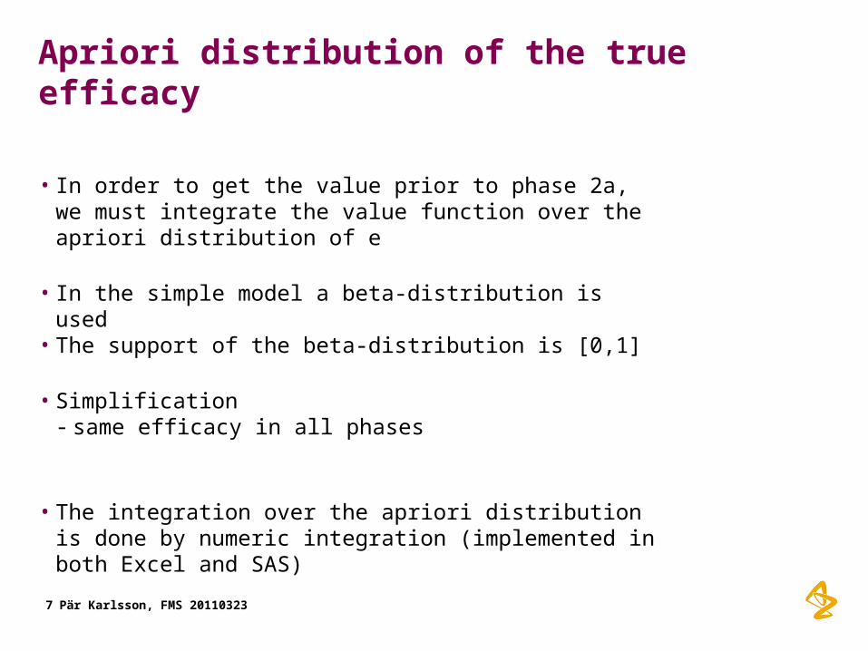
Apriori distribution of the true efficacy
• In order to get the value prior to phase 2a, we must integrate the value function over the apriori distribution of e
• In the simple model a beta-distribution is used• The support of the beta-distribution is [0,1]
• Simplification- same efficacy in all phases
• The integration over the apriori distribution is done by numeric integration (implemented in both Excel and SAS)
7 Pär Karlsson, FMS 20110323

Input / Output to the model
Pär Karlsson, FMS 201103238
Phase 2a Phase 2b Phase 3
Cost
Time
Type I error
Type II error
Probability of safety finding
Apriori distribution
Beta lower parameter
Beta upper parameter
Launch
End time of sales (from start of phase 2a)
Effect where sales begin to increase from zero
Effect where sales reach peak
Peak amount of sale
Output from the model
Expected cost
Expected value
Expected value / Expected cost

Results

Basic model
Input / Output to the model
Pär Karlsson, FMS 2011032310
Phase 2a Phase 2b Phase 3
Cost 10 25 100
Time 1 2 3
Type I error 0.05 0.05 0.025
Type II error 0.2 0.1 0.1
Probability of safety finding
0.2 0.1 0
Apriori distribution
Beta lower parameter 0
Beta upper parameter 0
Launch
End time of sales (from start of phase 2a)
12
Effect where sales begin to increase from zero
0.9
Effect where sales reach peak
0.9
Sales per year 1000
Output from the model
Expected cost 34.3
Expected value 184.4
Expected value / Expected cost 5.38

Power for the different studies
Phase 2bPhase 2a
Phase 3

Power for the different studies, adjusted for safety findings
Phase 2bPhase 2a
Phase 3

Power for the different studies, adjusted for safety findings, adding program power
Phase 2bPhase 2a
Phase 3
Phase 2
Phase 2 and 3

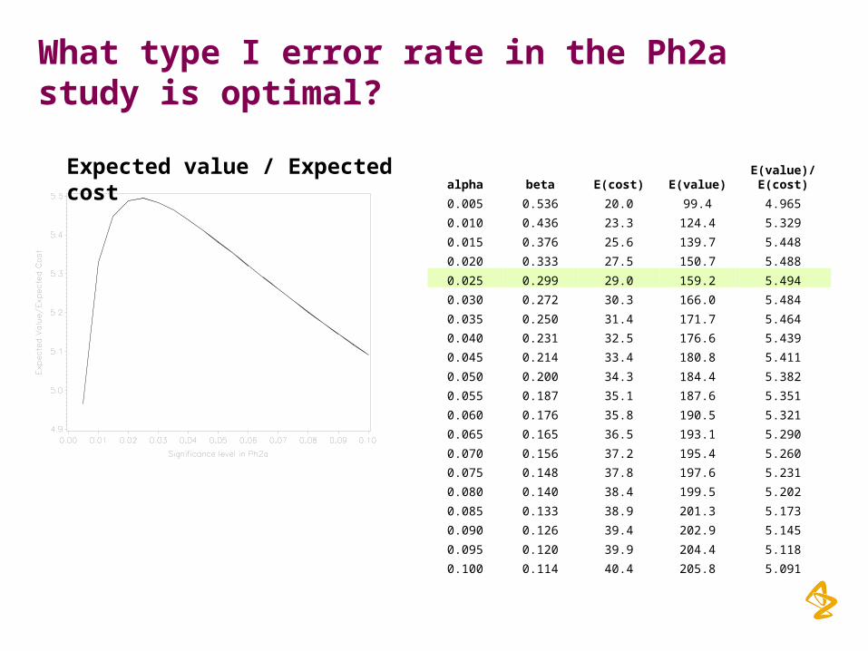
What type I error rate in the Ph2a study is optimal?
14 Pär Karlsson, FMS 20110323
Type I error
Type II error
0.01 0.44
0.03 0.27
0.05 0.20
0.10 0.11
0.15 0.07
0.20 0.05

What type I error rate in the Ph2a study is optimal?
Expected cost Expected value
What type I error rate in the Ph2a study is optimal?
Expected value / Expected costalpha beta E(cost) E(value)
E(value)/E(cost)
0.005 0.536 20.0 99.4 4.965
0.010 0.436 23.3 124.4 5.329
0.015 0.376 25.6 139.7 5.448
0.020 0.333 27.5 150.7 5.488
0.025 0.299 29.0 159.2 5.494
0.030 0.272 30.3 166.0 5.484
0.035 0.250 31.4 171.7 5.464
0.040 0.231 32.5 176.6 5.439
0.045 0.214 33.4 180.8 5.411
0.050 0.200 34.3 184.4 5.382
0.055 0.187 35.1 187.6 5.351
0.060 0.176 35.8 190.5 5.321
0.065 0.165 36.5 193.1 5.290
0.070 0.156 37.2 195.4 5.260
0.075 0.148 37.8 197.6 5.231
0.080 0.140 38.4 199.5 5.202
0.085 0.133 38.9 201.3 5.173
0.090 0.126 39.4 202.9 5.145
0.095 0.120 39.9 204.4 5.118
0.100 0.114 40.4 205.8 5.091
Is the optimal ph 2a type I error independent of apriori distribution?
Pär Karlsson, FMS 2011032317

Is the optimal ph 2a type I error independent of apriori distribution?
E = 0.333
E = 0.5
E = 0.667
apriori distributions

Is the optimal ph 2a type I error independent of apriori distribution?
alpha beta E =
0.333 E = 0.5E =
0.6670.005 0.536 -0.215 4.965 7.7590.010 0.436 -0.129 5.329 8.1080.015 0.376 -0.095 5.448 8.2040.020 0.333 -0.079 5.488 8.2250.025 0.299 -0.073 5.494 8.2160.030 0.272 -0.071 5.484 8.1930.035 0.250 -0.072 5.464 8.1630.040 0.231 -0.075 5.439 8.1290.045 0.214 -0.079 5.411 8.0940.050 0.200 -0.084 5.382 8.0590.055 0.187 -0.089 5.351 8.0230.060 0.176 -0.094 5.321 7.9880.065 0.165 -0.100 5.290 7.9540.070 0.156 -0.105 5.260 7.9210.075 0.148 -0.111 5.231 7.8880.080 0.140 -0.117 5.202 7.8570.085 0.133 -0.122 5.173 7.8260.090 0.126 -0.128 5.145 7.7960.095 0.120 -0.134 5.118 7.7670.100 0.114 -0.139 5.091 7.739
E = 0.333
E = 0.5
E = 0.667
Expected value / Expected cost

Is a phase 2a study a waste of money?
Pär Karlsson, FMS 2011032320
Phase 2a Phase 2b
Phase 3
Phase 3
Stop Stop Stop
Launch
Phase 2b
Phase 3
Phase 3
Stop Stop
Launch
Alternative with a phase 2a study
Alternative without a phase 2a study

Is a phase 2a study a waste of money?
Input to the model
Pär Karlsson, FMS 2011032321
Phase 2a Phase 2b Phase 3
Cost 10 or 0 25 100
Time 1 or 0 2 3
Type I error 0.05 or 1 0.05 0.025
Type II error 0.2 or 0 0.1 0.1
Probability of safety finding
0.2 0.1 0
Apriori distribution
Beta lower parameter 1 to 0
Beta upper parameter 0 to 1
Launch
End time of sales (from start of phase 2a)
12
Effect where sales begin to increase from zero
0.9
Effect where sales reach peak
0.9
Sales per year 1000

Apriori distributions
Lower parameter
Upper parameter
Expected value
0 1 0.3330.2 1 0.3750.5 1 0.4291 1 0.5001 0.5 0.5711 0.2 0.6251 0 0.667
Apriori distributions

Is a phase 2a study a waste of money?
Expected cost Expected value

Is a phase 2a study a waste of money?
Expected value / Expected cost
No ! not with these assumptions
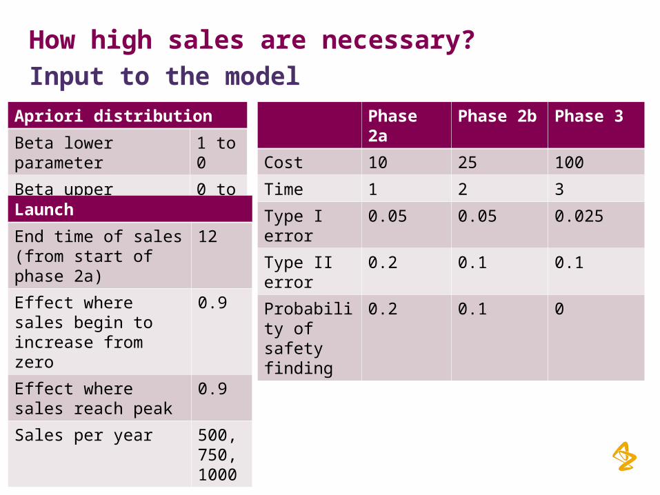
How high sales are necessary?
Input to the model
Pär Karlsson, FMS 2011032325
Phase 2a Phase 2b Phase 3
Cost 10 25 100
Time 1 2 3
Type I error 0.05 0.05 0.025
Type II error 0.2 0.1 0.1
Probability of safety finding
0.2 0.1 0
Apriori distribution
Beta lower parameter 1 to 0
Beta upper parameter 0 to 1
Launch
End time of sales (from start of phase 2a)
12
Effect where sales begin to increase from zero
0.9
Effect where sales reach peak
0.9
Sales per year 500, 750, 1000

Apriori distributions
Lower parameter
Upper parameter
Expected value
0 1 0.3330.2 1 0.3750.5 1 0.4291 1 0.5001 0.5 0.5711 0.2 0.6251 0 0.667
Apriori distributions
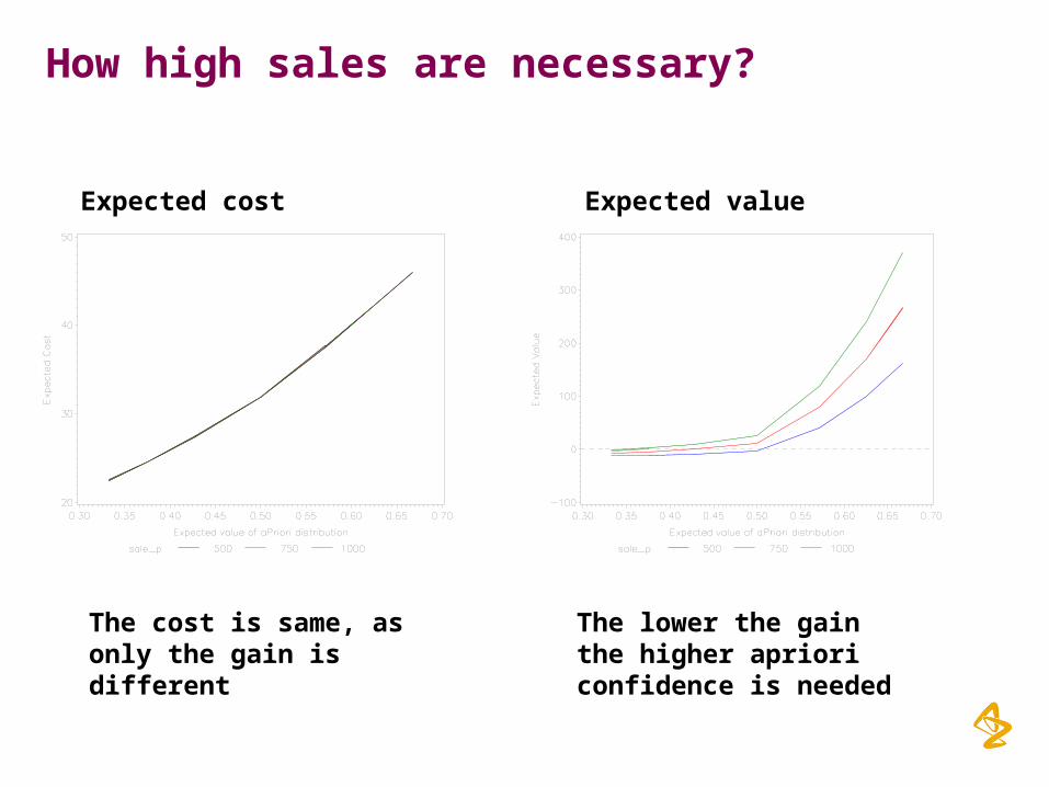
How high sales are necessary?
Expected cost Expected value
The cost is same, as only the gain is different
The lower the gain the higher apriori confidence is needed

How high sales are necessary?
Expected value / Expected cost
Note, that for this question it is enough to look at the expected value, as the important point is when the lines cross zero

Summary

Summary
• A simple model of the drug development has been developed
• Some important questions can be addressed
• As the model is simple, a more complete/complicated model should be developed
• The main purpose is to inspire statisticians to improve the development processes of drug development
Pär Karlsson, FMS 2011032330