pär lindahl- energy calibration of neutrino telescopes using ultra high energy tau neutrinos
TRANSCRIPT

8/3/2019 Pär Lindahl- Energy Calibration of Neutrino Telescopes Using Ultra High Energy Tau Neutrinos
http://slidepdf.com/reader/full/paer-lindahl-energy-calibration-of-neutrino-telescopes-using-ultra-high-energy 1/81
Energy Calibration of Neutrino Telescopes
Using
Ultra High Energy Tau Neutrinos
Licentiate Thesisby Pär Lindahl
Stockholm University, Department of Physics
and
Kalmar University, Department of Technology
2003

8/3/2019 Pär Lindahl- Energy Calibration of Neutrino Telescopes Using Ultra High Energy Tau Neutrinos
http://slidepdf.com/reader/full/paer-lindahl-energy-calibration-of-neutrino-telescopes-using-ultra-high-energy 2/81

8/3/2019 Pär Lindahl- Energy Calibration of Neutrino Telescopes Using Ultra High Energy Tau Neutrinos
http://slidepdf.com/reader/full/paer-lindahl-energy-calibration-of-neutrino-telescopes-using-ultra-high-energy 3/81
--- iii ---
To Pia and David with love!

8/3/2019 Pär Lindahl- Energy Calibration of Neutrino Telescopes Using Ultra High Energy Tau Neutrinos
http://slidepdf.com/reader/full/paer-lindahl-energy-calibration-of-neutrino-telescopes-using-ultra-high-energy 4/81
--- iv ---
Contents
1 Introduction ........................................................................................................................... 1
2 High-energy neutrinos .......................................................................................................... 3
2.1 Scientific motivation for neutrino astronomy .................................................................. 3
2.2 Neutrino sources............................................................................................................... 4
2.2.1 Dark matter annihilation............................................................................................ 4
2.2.2 Cosmic-ray interactions............................................................................................. 4
2.2.3 Gamma-ray bursters.................................................................................................. 5
2.2.4 Active galactic nuclei ................................................................................................ 6
2.2.5 Topological defects ................................................................................................... 62.3 Neutrino oscillation .......................................................................................................... 6
2.4 Neutrino interactions ........................................................................................................ 8
2.4.1 Neutrino + nucleon cross-sections ............................................................................ 8
2.4.2 Earth shielding at high energies ................................................................................ 9
2.5 Flux estimations ............................................................................................................. 12
3 Neutrino telescopy with the AMANDA and IceCube detectors...................................... 14
3.1 Principle of detection ..................................................................................................... 14
3.2 Ice properties ..................................................................................................................17
3.3 Optical modules.............................................................................................................. 19
3.4 Signal transmission and amplification ........................................................................... 20
3.5 The trigger ...................................................................................................................... 21
4 Investigation of detector properties...................................................................................23
4.1 Detector simulation with electra .................................................................................... 23
4.1.1 Motivation ...............................................................................................................23
4.1.2 Description .............................................................................................................. 23
4.2 An all-channel survey for AMANDA-B13.................................................................... 24
4.2.1 Introduction ............................................................................................................. 24
4.2.2 High voltage settings............................................................................................... 25
4.2.3 Pulse rates................................................................................................................ 26
4.2.4 Pulse shapes............................................................................................................. 28
4.2.5 Noise, cross-talk and external pick-up .................................................................... 30
4.2.6 SWAMP gain and delay.......................................................................................... 31
5 Cascade-like events ............................................................................................................. 34 5.1 Intrinsic cascade properties ............................................................................................ 34
5.1.1 General properties ................................................................................................... 34
5.1.2 Electromagnetic cascades........................................................................................ 35
5.1.3 Hadronic cascades ................................................................................................... 36
5.2 Cascade detection........................................................................................................... 36
5.2.1 Introduction ............................................................................................................. 36
5.2.2 Reconstruction of position and time........................................................................ 37
5.2.3 Reconstruction of energy and direction .................................................................. 37

8/3/2019 Pär Lindahl- Energy Calibration of Neutrino Telescopes Using Ultra High Energy Tau Neutrinos
http://slidepdf.com/reader/full/paer-lindahl-energy-calibration-of-neutrino-telescopes-using-ultra-high-energy 5/81
--- v ---
5.2.4 Reconstruction performance ...................................................................................37
6 Detection of tau neutrinos................................................................................................... 39
6.1 The double bang signature ............................................................................................. 39
6.1.1 Overview.................................................................................................................39
6.1.2 The neutrino-nucleon reaction ................................................................................40
6.1.3 The tauon propagation............................................................................................. 41
6.1.4 The tauon decay ...................................................................................................... 426.2 Detection criteria ............................................................................................................ 43
7 Simulation- and analysis tools............................................................................................ 44
7.1 Overview ........................................................................................................................ 44
7.2 Event generator ..............................................................................................................45
7.3 Detector simulation ........................................................................................................ 46
7.4 Analysis programs.......................................................................................................... 47
8 Intrinsic properties of double bang events........................................................................ 48
8.1 Motivation ......................................................................................................................48
8.2 Simulations..................................................................................................................... 48
8.3 Results ............................................................................................................................ 49
8.3.1 Visible energy — first cascade................................................................................49
8.3.2 Visible energy — second cascade........................................................................... 508.3.3 Inelasticity ............................................................................................................... 51
8.3.4 Tauon range ............................................................................................................. 52
9 Anticipated event rates ....................................................................................................... 53
9.1 Motivation ......................................................................................................................53
9.2 Double bang production rate .......................................................................................... 53
9.2.1 Model ...................................................................................................................... 53
9.2.2 Simulations .............................................................................................................. 54
9.2.3 Result....................................................................................................................... 55
9.3 Effective volume ............................................................................................................ 56
9.3.1 Model ...................................................................................................................... 56
9.3.2 Simulations .............................................................................................................. 56
9.3.3 Results .....................................................................................................................57
9.4 Event rate calculations ................................................................................................... 58
9.5 Conclusions ....................................................................................................................59
10 Energy calibration............................................................................................................. 61
10.1 Motivation .................................................................................................................... 61
10.2 Method ......................................................................................................................... 62
10.2.1 Energy estimation.................................................................................................. 62
10.2.2 Simulation ............................................................................................................. 64
10.2.3 Analysis ................................................................................................................. 65
10.3 Results .......................................................................................................................... 65
10.3.1 Calibration performance........................................................................................ 65
11 Summary and outlook....................................................................................................... 67 Acknowledgements................................................................................................................. 71
Bibliography ........................................................................................................................... 72
List of Publications for Pär Lindahl..................................................................................... 75

8/3/2019 Pär Lindahl- Energy Calibration of Neutrino Telescopes Using Ultra High Energy Tau Neutrinos
http://slidepdf.com/reader/full/paer-lindahl-energy-calibration-of-neutrino-telescopes-using-ultra-high-energy 6/81
--- 1 ---
Chapter 1
Introduction
High-energy neutrinos have the potential to convey information from the edge of the universe
and from deep inside the most cataclysmic high-energy processes. These particles may also
reveal the presence of the elusive “dark matter”, which is suspected to contribute the
dominating portion of the mass density on cosmic scales. By recent development of the firstgeneration of high-energy neutrino telescopes a new promising “window” has been opened
toward the universe.
The largest existing and future neutrino telescopes are designed to detect the Čerenkov
photons emitted by charged particles produced as a result of neutrino-nucleon reactions. The
detector medium for these detectors is naturally occurring water (BAIKAL [1], ANTARES
[2], NESTOR [3] and NEMO [4]) or ice (AMANDA [5] and IceCube [6]).
Several features of the interacting neutrino may be derived from the detection of Čerenkov
photons propagating through the detector volume. These features include direction-of-origin
and energy of the neutrino. However, since this is an indirect measurement — the detected
particles are the daughters of a neutrino-nucleon interaction — it is appropriate to separate the
analysis of an event into two parts: First the relevant properties of the charged particles are
determined. Then these results are used to derive information about the parent neutrino.
To be able to perform the first step one needs to calibrate the detector. This involves
detailed investigations determining the properties of the different subsystems and how they
interact with each other. The second step, which is an interpretation of the measurement,
depends on knowledge about the neutrino-nucleon interaction and on the expected neutrino
flux.
In this thesis I propose a method for energy calibration of neutrino telescopes. In contrast
to accelerator based experiments, in which a detector may be calibrated by exposing it to a beam with known composition and energy and then measure its response, the calibration of
the neutrino telescopes discussed here is more dependent on detailed simulations of every part
of the detection process. This includes particle reactions in the material inside and
surrounding the detector, photon propagation through the detector medium, photon detection
and the response of the accompanying electronics.

8/3/2019 Pär Lindahl- Energy Calibration of Neutrino Telescopes Using Ultra High Energy Tau Neutrinos
http://slidepdf.com/reader/full/paer-lindahl-energy-calibration-of-neutrino-telescopes-using-ultra-high-energy 7/81
--- 2 ---
To determine the validity of the simulation results it would of course be advantageous if
one could identify a subset of reactions in the detector where the energy deposit can be
determined by some independent method. This subset could then be used for calibration in a
similar fashion as with a man-made calibration beam. In this thesis I investigate the possibility
to use one such subset, described by the so-called ”double bang signature” [7], two particle
cascades separated by the flight of a relativistic tauon. The first cascade and the appearance of
the tauon is the result of a charged current (CC) tau neutrino reaction with a nucleon. Thesecond cascade is the result of the tauon decay. Since the tauon decays in flight its mean range
is proportional to its energy — a fact useful for calibration purposes.
In the proposed calibration scheme one uses reconstructed cascade separations for a set of
double bang events to estimate the corresponding second-cascade energy deposits. For each
event one also reconstructs the energy deposit using the default algorithm for the detector. An
important cross-check for this algorithm may then be obtained by comparing the two sets of
energy estimations.
To be able to evaluate the prospects for this calibration method one needs to address three
questions:
1) Are tau neutrinos of sufficient energy (∼1 PeV) produced in nature?• An outline of the theoretical and experimental indications is presented in chapter 2.
2) If tau neutrinos are produced in nature, under what conditions will the present or planned
neutrino telescopes be able to detect them?
• In chapters 3 and 4 the AMANDA and IceCube detectors are presented, including a
description of a work regarding the properties of the detector electronics in AMANDA.
• In chapters 5, 6, 8 and 9 the double bang signature and its detection are described in
some detail.
3) If tau neutrinos are detected, under what conditions can the double bang signature be used
for calibration purposes?
• In chapter 10 I present an investigation of the calibration method using simulated
double bang events.• In chapter 7 I present all simulation tools used for generation of tau neutrinos,
simulation of the detector response and for the subsequent analysis of the double bang
events.
The final chapter of this thesis, chapter 11, contains a summary and an outlook towards
future investigations.

8/3/2019 Pär Lindahl- Energy Calibration of Neutrino Telescopes Using Ultra High Energy Tau Neutrinos
http://slidepdf.com/reader/full/paer-lindahl-energy-calibration-of-neutrino-telescopes-using-ultra-high-energy 8/81
--- 3 ---
Chapter 2
High-energy neutrinos
2.1 Scientific motivation for neutrino astronomy
With the advent of neutrino telescopes sensitive in the highest energy range, a new window is
opened to the universe. Several questions in particle physics and astrophysics may be
addressed through observations that are complementary (and supportive) to other detection
methods.
Many proposed sources of high-energy neutrinos will also emit gamma rays and various
charged particles. If the charged particles encounter any electric or magnetic fields as they
propagate through space they will be deflected, thus potentially loosing the information about
their direction of origin. The electrically neutral gamma rays and neutrinos, on the other hand,
will travel in straight lines (i.e. along geodesics). However, with increasing energy, the cross-
section increases for gamma rays to interact, predominantly through pair production with thelow-energy photons constituting the cosmic microwave background radiation (CMBR). This
attenuation limits the accessible range for gamma-ray telescopy, and also modifies the
gamma-ray spectrum. Neutrinos do not suffer from these limitations, since they only interact
through the weak force (and gravity). This fact also allows neutrinos to escape from dense
regions that are obscured for other types of radiation.
Through high-energy neutrino astronomy it may be possible to investigate the nature of the
dark matter, to search for the origin of the cosmic rays, to probe the physical processes
responsible for the energy release in the most luminous objects in the universe, and to study
the phenomenon of neutrino oscillation between flavors. In addition, there is also the very real
possibility to unveil something completely unexpected, as has happened before when new
observation methods has been introduced.
In this chapter a few potential sources for high-energy neutrinos are presented, followed
by introductions to some effects of neutrino oscillation and neutrino interaction with matter.
Finally, the expected neutrino flux is indicated through a few examples on theoretical flux
estimations and experimental upper limits.

8/3/2019 Pär Lindahl- Energy Calibration of Neutrino Telescopes Using Ultra High Energy Tau Neutrinos
http://slidepdf.com/reader/full/paer-lindahl-energy-calibration-of-neutrino-telescopes-using-ultra-high-energy 9/81
--- 4 ---
2.2 Neutrino sources
2.2.1 Dark matter annihilation
Studies of the anisotropy of the CMBR [8] and of the magnitude-redshift distribution for
Ia-type super-novae [9] suggest that dark matter constitute close to 83% of the matter in the
universe [10]. Dark matter only manifests itself through its gravitational influence on its
surroundings. Its nature is not known, but candidates are generically labeled “hot” for
relativistic constituents or “cold” for non-relativistic ones.
One group of particles among the cold-dark-matter candidates is the weakly interacting massive particles (WIMPs), whose existence is proposed by some supersymmetric theories.
These particles may have been gravitationally trapped inside massive astronomical bodies,
like the Sun or the Earth, leading to increased annihilation rates at these sites [11]. The
particles produced in the annihilation process will decay. Among the decay products therewill be neutrinos, with a broad energy spectrum bounded from above by the WIMP mass.
Cosmological arguments suggest that such cold dark matter candidates should have a mass
below ∼10 TeV [11].
The search for a neutrino signal from the Sun or the Earth at energies compatible with the
WIMP models will contribute both to fundamental particle physics and to cosmology.
2.2.2 Cosmic-ray interactions
The cosmic rays mainly consist of light nuclei, with a very broad energy range. The flux of
these particles has been measured over many decades in energy, and the differential energy
spectrum can be described by a segmented power-law formula [12]
α −∝ CR
CR
CR
d
d E
E
N (2.1)
with the following values for the spectral index:
=0.3
7.2α
eV1010
eV10
1816
16
<<
<
E
E (2.2)
Above 1018 eV the spectral index appears to be somewhat smaller. (Observations extend to
energies above 1020
eV.)
The origin of the cosmic rays is not known, mainly due to the fact that the interstellar
magnetic field within our galaxy deflects these charged particles. It is therefore difficult to
associate them with any particular point (object) in the sky. It is, however, known that the
sources for the most energetic cosmic-ray particles cannot be arbitrarily distant. This is due to
attenuation: Regardless of its nature, cosmic-ray particles above 1019
eV will interact,
predominantly with the CMBR, making the universe opaque at distances larger than
∼100 Mpc [13]. Due to the energy dependence of the attenuation, the observed cosmic-ray
spectrum is steeper than the emitted spectrum.

8/3/2019 Pär Lindahl- Energy Calibration of Neutrino Telescopes Using Ultra High Energy Tau Neutrinos
http://slidepdf.com/reader/full/paer-lindahl-energy-calibration-of-neutrino-telescopes-using-ultra-high-energy 10/81
--- 5 ---
From the cosmic-ray sources also neutrinos will emerge, and this flux will be less
affected by the interstellar and intergalactic media: There will be less attenuation, allowing
neutrinos to reach us from the entire observable universe. Also, the neutrino spectrum will
suffer less distortion (and will thus be more “flat”) than the cosmic-ray spectrum.
In addition to the direct neutrino emission from the cosmic-ray sources, the cosmic rays
will produce neutrinos as a result of interactions with various matter- and radiation targets.Matter targets include the interstellar matter in the galactic disk, the Sun and the Earth’s
atmosphere. An important radiation target is the CMBR. Since the most common cosmic-ray
particle is the proton, the neutrino production may be exemplified by considering the result
from p + p or p + γ interactions. In these processes large amounts of pions will be produced.
The neutral pion will decay into two photons, and the charged pions will follow the decay
chain*: π → µ + ν µ followed by µ → ν µ + e + ν e. This scenario suggests that muon neutrinos
are twise as abundant as electron neutrinos [14]. For a “thin” target the majority of the pions
will decay (and produce neutrinos) instead of further interacting with the target material. The
neutrino spectrum for such a target will thus follow the shape of the cosmic-ray spectrum. For
“dense” targets, interactions with the target will compete with decay, especially at higher
energies, thus producing a steeper neutrino spectrum.
Some of the neutrino-flux components from cosmic-ray interactions with known targets
can be calculated, and may serve as reference fluxes. The hope is to be able to identify some
high-energy neutrino point sources above this “background”, indicating the possible cosmic-
ray sources. But even if these sources would turn out to be too weak neutrino emitters to be
individually identified, the calorimetric information from their collective flux would (if it
could be measured) provide important information about the nature of these sources.
2.2.3 Gamma-ray bursters
A flux of high-energy hadrons (possible primaries for high-energy neutrino production) may
be produced through either direct acceleration of such particles (“bottom-up” production) or
through hadronic decay of extremely massive particles (“top-down” production). A number of
phenomena involving acceleration are known today. The most luminous of these is the
gamma-ray burst (GRB), which are events (of extragalactic origin) lasting between a few tens
of milliseconds to a few hundred seconds [12].
One plausible model for the GRBs is the “relativistic fireball model” by Meszárós & Rees
(see e.g. [15]) in which gravitational energy is released through the collapse of a massive star
or the merging of two star remnants (neutron stars and/or black holes). The collapse/merging
is followed by an ultra-relativistic expansion. Accelerated electrons will produce gamma rays
through synchrotron radiation, and as the plasma becomes transparent the gamma rays arereleased. Also protons will be accelerated, and pions will be produced in the following p + γ
interactions. In turn, the pions will decay and thus produce neutrinos.
*No distinction has been made between a particle and its antiparticle.

8/3/2019 Pär Lindahl- Energy Calibration of Neutrino Telescopes Using Ultra High Energy Tau Neutrinos
http://slidepdf.com/reader/full/paer-lindahl-energy-calibration-of-neutrino-telescopes-using-ultra-high-energy 11/81
--- 6 ---
The theoretical framework for describing acceleration of particles associated with
supersonic shocks in a plasma is called “Fermi acceleration” [16]. The differential energy
spectrum for the accelerated charged particles, and thus of the produced gamma rays and
neutrinos, can be described by a power-law formula. The typical value for the spectral index
is 2=α . Thus, for neutrinos
2
ν
ν
ν
d
d −∝ E E
N . (2.3)
2.2.4 Active galactic nuclei
Roughly 1% of all galaxies possess an active nucleus, from which more power is emitted than
e.g. the collective radiation from all the stars in our galaxy. It is believed that these active galactic nuclei (AGN) are powered by super-massive black holes, causing acceleration and
accretion of surrounding material [15]. In these processes strong shocks are formed, leading to
Fermi acceleration of charged particles.
If protons are among the accelerated particles they will produce pions through
""anything p p +→→+ ±π L or ++ +→∆→+ π γ n p interactions, and neutrinos will
emerge as the pions decay.
2.2.5 Topological defects
Both GRB:s and AGN:s could produce the most energetic cosmic-ray particles through
acceleration of charged particles (bottom-up production). An alternative mechanism to
produce these cosmic-ray particles is through hadronic decay of extremely massive (GUT
scale: ∼1024 eV) particles (top-down production). Such massive particles may be produced by
radiation, interaction or collapse of “topological defects” like monopoles, cosmic strings, etc
[13] [17].
2.3 Neutrino oscillation
Neutrinos produced in p + p or p + γ interactions are not evenly distributed between the three
neutrino flavors. According to what has been pointed out in section 2.2.2 muon neutrinos and
electron neutrinos are the products of charged-pion decays, with twice as manymuon neutrinos as electron neutrinos. The main source for “prompt” tau neutrinos is the decay
of charged±S D mesons [14]. However, the cross-section for
±S D production is ∼4 orders of
magnitude smaller than that of charged-pion production. In addition tau neutrinos are only
produced in ∼3% of the ±S D decays [18]. Thus, the expected flavor mix from these sites is
(roughly) 1:2:<10-5
for electron neutrinos, muon neutrinos and tau neutrinos respectively.

8/3/2019 Pär Lindahl- Energy Calibration of Neutrino Telescopes Using Ultra High Energy Tau Neutrinos
http://slidepdf.com/reader/full/paer-lindahl-energy-calibration-of-neutrino-telescopes-using-ultra-high-energy 12/81
--- 7 ---
Even if only a very small fraction of the neutrinos produced in the universe are
tau neutrinos – due to so-called called “neutrino mixing” – all three neutrino flavors will be
equally abundant since neutrinos are oscillating between flavors as they propagate., This was
first shown by the Super-Kamiokande collaboration [19], and a consequence of their result is
that half of the generated muon neutrinos within any sufficiently large energy interval will
have converted into tau neutrinos before reaching Earth:
The probability for a muon neutrino ( µν ) of energy ν E to be converted into a tau neutrino
( τ ν ) at a distance x from the source is given by
=→ π
E L
xνν P
νν
τ µ)(
sin)2(sin)( 22 θ (2.4)
(see for example [12]) where θ is the mixing angle, and the oscillation length for the mass-
difference squared 222
µτ νν mmm −=∆ is
∆
⋅=∆
=2
423
32
/eV1
GeV11048.2
2)(
m
c E
cm
h E E L νν
νν meters. (2.5)
Results from the Super-Kamiokande experiment indicate that oscillation betweenmuon neutrinos and tau neutrinos takes place with near maximal mixing, 1)2(sin
2 =θ , with a
favored mass-difference squared of 32
102.3−⋅=∆m )/(eV
42 c [19]. The corresponding
oscillation length according to equation (2.5) is
⋅=
GeV1108.7)( 5 ν
νν
E E L meters
⋅= −
PeV1102.8 5 ν E
light-years. (2.6)
For a source at a fixed distance )( νν E L x >> the conversion probability according to equation
(2.4) is a rapidly oscillating function with energy. By inserting equation (2.6) into (2.4) the
energy separation between two minima can be approximated by a continuous function:2
5
PeV1
ly1
102.8)(
⋅≈∆
− ν
ν
E
x E E PeV, (2.7)
where ν E is in the interval between the two minima.
If E ∆ is much smaller than the energy resolution ( E σ ) of the detector, the conversion
probability averaged over some appropriate energy interval (centered at ν E ) may be used as
an effective conversion probability. Assuming a slowly varying energy spectrum this effective
conversion probability is given by
≈→>==< ∫ +
−
E
E
E
σ E
σ E
ντ µσ νν E νν P E P E P ν
ν
d)()()( 21
eff
)2(sin2
2
1 θ ≈ ; )νν(E L x >> , E σ E ∆>> , (2.8)
i.e. a constant, only depending on the mixing angle.

8/3/2019 Pär Lindahl- Energy Calibration of Neutrino Telescopes Using Ultra High Energy Tau Neutrinos
http://slidepdf.com/reader/full/paer-lindahl-energy-calibration-of-neutrino-telescopes-using-ultra-high-energy 13/81
--- 8 ---
This thesis focuses on the possible detection of tau neutrinos, with their energies in the
interval PeV100PeV1 << ν E , through the so-called “double bang” signature (presented in
section 6.1). According to equation (2.6) the oscillation length ly10)PeV100( 2−≈ν L , which
is much less than the distance to the closest star, α Centauri, at 4.3 ly. For a neutrino source at
ly4≈ x the energy separation between probability minima according to equation (2.7) is
PeV2.0)100( ≈∆ PeV E , which is much smaller than the achievable energy resolution atthese neutrino energies (see section 5.2.4). Thus, at ultra-high energies (UHE) the
requirements of equation (2.8) are fulfilled for any neutrino sources “outside” the solar system
(i.e. at distances greater than that of the closest stars).
Resent results [20] and [21] show that electron neutrinos also participate in the oscillation
scenario. All three neutrino flavors are thus involved in this phenomenon. In the estimations
of the expected tau neutrino detection rates presented in chapter 9 it is assumed that, due to
oscillation between neutrino flavors, one third of all UHE neutrinos (from distant sources) are
tau neutrinos.
2.4 Neutrino interactions
2.4.1 Neutrino + nucleon cross-sections
Neutrinos interact with quarks and leptons through the weak force, which is mediated by
either an electrically charged particle, the W ±, (charged current (CC) interaction) or a neutral
particle, the Z 0, (neutral current (NC) interaction). The cross-section for these reactions is
very small. This allows neutrinos to travel over cosmological distances without scattering. On
the other hand, the low interaction probability imposes a need for very large detectors, to be
able to reach a reasonably high detection rate.
As neutrinos encounter a matter target reactions will take place with both electrons and
nucleons. However, for neutrinos with energies in the range PeV100PeV1 ≤≤ ν E the cross-
section for ν + e reactions is very small compared with the cross-section for ν + nucleon
reactions*. Therefore, only reactions with nucleons will be considered here.
With the nucleons at rest, the cross-section increases monotonically with neutrino energy
as smaller details of the internal structure of the nucleon become “visible” to the neutrino. At
low energies the cross-section may be measured experimentally, but to estimate the cross-
section at higher energies one is forced to make extrapolations. One modern set of CC and NCcross-section estimates is presented in [22]. These cross-sections are shown in figure 2.1 for a
broad energy range. It may be noted that no distinction has been made between the three
neutrino flavors, since their cross-sections are all expected to be very similar at these energies.
Furthermore, the cross-sections for neutrino- and antineutrino reactions are similar, and the
difference will be neglected here.
*The only exception is the “resonance” at 6.3 PeV for ee +ν reactions.

8/3/2019 Pär Lindahl- Energy Calibration of Neutrino Telescopes Using Ultra High Energy Tau Neutrinos
http://slidepdf.com/reader/full/paer-lindahl-energy-calibration-of-neutrino-telescopes-using-ultra-high-energy 14/81
--- 9 ---
Also shown in figure 2.1 is a suggested parameterization for the total cross section ( totσ ).
This parameterization was obtained by minimizing the relative error compared with the
estimates in [22] over the presented energy interval:49.0
1totPeV1
)(
= ν ν σ σ
E E ;
38
1 108 −⋅=σ m2
(2.9)
Neutrino + Nucleon C ross-section
1,0E-39
1,0E-38
1,0E-37
1,0E-36
0,01 0,1 1 10 100
E ν
[PeV]
σ [ m
2 ]
Figure 2.1ν + nucleon cross-section estimates, calculated using the CTEQ4-DIS parton distributions [22].Squares indicate NC cross-sections, triangles CC cross-sections and circles total (NC+CC) cross-sections. Also
included in this plot is a suggested parameterization for the total cross-section: σ tot( E ν ) = 8⋅10-38
( E ν /1PeV)0.49
m2.
2.4.2 Earth shielding at high energies
One notable effect of the increasing cross-section with energy is that above some energy the
Earth can no longer be regarded as transparent to neutrinos. This effect results in a reduced
neutrino flux from “below” at high energies.

8/3/2019 Pär Lindahl- Energy Calibration of Neutrino Telescopes Using Ultra High Energy Tau Neutrinos
http://slidepdf.com/reader/full/paer-lindahl-energy-calibration-of-neutrino-telescopes-using-ultra-high-energy 15/81
--- 10 ---
In [24] one defines by the transparency energy ( E tr ) — the energy where the neutrino
range is equal to the distance through the Earth along the trajectory towards the detector. This
distance varies with nadir angle (θ ), and so does the transparency energy. Under the
approximations that the Earth may be regarded as a homogenous sphere with radius6104.6 ⋅≈⊕ R m and density 3105.5 ⋅≈⊕ ρ kg/m
3, and using the parameterization of the total
cross-section according to equation (2.9), the transparency energy is expressed by49.0/1
A1
tr cos2
1
⋅⋅⋅⋅=
⊕⊕ N R E
ρ σ θ PeV, (2.10)
where26
A 100.6 ⋅≈ N kg-1
is the Avogadro constant.
As a neutrino interacts inside our planet it will loose some of its energy (or all, if no
neutrino is among the daughters of the reaction). In NC reactions the neutrino will scatter
(inelastically) against the nucleon in the same way for all types of neutrinos. In CC reactions
(which are roughly twice as likely) the neutrino is converted into the corresponding charged
lepton, with different results for the three flavors:
For an initial electron neutino an electron is created, which is rapidly brought to rest inmatter. The electron is stable, and there will be no “secondary” neutrinos.
For an initial muon neutrino a muon is created. This lepton subsequently decays,
producing a muon neutrino, an electron and an electron neutrino. However, before decaying
the muon will propagate through matter. As its range in matter is much smaller than its decay
length, it will loose most of its energy (through electromagnetic interactions) before decaying.
The energy of the “secondary” neutrinos will therefore be well below the energy threshold of
any high-energy neutrino telescope.
For an initial tau neutrino a tauon is created. This lepton decays through one of a large
number of possible decay modes. There will however always be a tau neutrino present among
the decay products. The lifetime of the tauon is much smaller than that of a muon (the decaymay be regarded as essentially “prompt”), and the “secondary” neutrino(s) will be left with a
substantial fraction of the initial energy. The Earth is therefore not entirely opaque to
tau neutrinos above the transparency energy, but the energy of such neutrinos will be reduced.
According to [24] the result will be a peak in the tau neutrino energy spectrum around the
transparency energy. This peak characteristically follows a lognormal distribution, with a log
scale r.m.s. width corresponding to approximately one decade in energy.
To make a rough estimate regarding the detectable tau neutrino flux from below one has
to compare the transparency energy with the energy threshold of the detector. According to
equation (2.10) the transparency energy at θ = 0° is ∼0.08 PeV. For a detector with its
threshold well above this energy, say at E th = 1 PeV, the “peak” in the spectrum will not enter
the sensitive region. As a “first order approximation” (for such a detector) one may thereforeregard the Earth as effectively opaque to tau neutrinos from “below”. In other words: 50% of
the tau neutrino sky is shielded off by the Earth.

8/3/2019 Pär Lindahl- Energy Calibration of Neutrino Telescopes Using Ultra High Energy Tau Neutrinos
http://slidepdf.com/reader/full/paer-lindahl-energy-calibration-of-neutrino-telescopes-using-ultra-high-energy 16/81
--- 11 ---
One approach to find a “second order approximation” (also including angular effects) is
to assume that the Earth is opaque to tau neutrinos at nadir angles smaller than a certain
boundary value, and transparent for larger values. Given this boundary angle ( boundaryθ ) it is
then straightforward to calculate how much of the sky that would be shielded off by the Earth:
2
cos1
sr 4
boundaryθ
π
ϖ −= , (2.11)
where ϖ is the solid angle shielded off by the Earth.
For small nadir angles the peak in the energy spectrum is below the threshold of the
detector, and the Earth is effectively opaque to tau neutrinos. For sufficiently large angles the
peak will be positioned within (or above) the energy interval where the detector is sensitive,
and the Earth may be regarded as transparent. In the present context it seems reasonable to
select a boundary angle for which the corresponding transparency energy ( boundary
tr E ) is similar
to the threshold of the detector. Using equation (2.10) the “shielding fraction” (the fraction of
the sky shielded off by the Earth) may now be given as a function of this energy:
( )
⋅⋅⋅−=
⊕⊕
−
A1
49.0 boundary
tr
2
1
2
1
sr 4 N R
E
ρ σ π
ϖ (2.11’)
In figure 2.2 the shielding fraction according to equation (2.11’) is presented. From this
plot it is apparent that, assuming PeV1PeV1 boundary
tr th ≈⇒≈ E E , ∼35% of the sky is
shielded off by the Earth. Thus, the first- and second order approximations yield similar
results.
Shielding Fraction
0%
5%
10%
15%
20%
25%
30%
35%
40%
45%
50%
0,01 0,1 1 10 100
E tr boundary [PeV]
/ 4
Figure 2.2 Fraction of the tau neutrino sky shielded off by the Earth. This fraction is presented as a function of
the particular transparency energy ( E tr boundary
) that defines the boundary between nadir angles where the planet is
(effectively) opaque and (effectively) transparent. Presumably this boundary energy is similar to the energy
threshold ( E th) of the detector.
8/3/2019 Pär Lindahl- Energy Calibration of Neutrino Telescopes Using Ultra High Energy Tau Neutrinos
http://slidepdf.com/reader/full/paer-lindahl-energy-calibration-of-neutrino-telescopes-using-ultra-high-energy 17/81
--- 12 ---
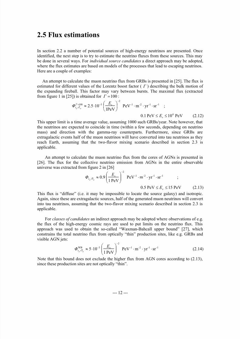
2.5 Flux estimations
In section 2.2 a number of potential sources of high-energy neutrinos are presented. Once
identified, the next step is to try to estimate the neutrino fluxes from these sources. This may
be done in several ways. For individual source candidates a direct approach may be adopted,where the flux estimates are based on models of the processes that lead to escaping neutrinos.
Here are a couple of examples:
An attempt to calculate the muon neutrino flux from GRBs is presented in [25]. The flux is
estimated for different values of the Lorentz boost factor ( Γ ) describing the bulk motion of
the expanding fireball. This factor may vary between bursts. The maximal flux (extracted
from figure 1 in [25]) is obtained for 100= Γ :2
3100
PeV1105.2
−−=
+
⋅≈ ν Γ
νν
E Φ
µ µ -1-1-2-1 sr yr mPeV ⋅⋅⋅ ;
PeV10PeV1.0 4≤≤ ν E (2.12)
This upper limit is a time average value, assuming 1000 such GRBs/year. Note however, that
the neutrinos are expected to coincide in time (within a few seconds, depending on neutrino
mass) and direction with the gamma-ray counterparts. Furthermore, since GRBs are
extragalactic events half of the muon neutrinos will have converted into tau neutrinos as they
reach Earth, assuming that the two-flavor mixing scenario described in section 2.3 is
applicable.
An attempt to calculate the muon neutrino flux from the cores of AGNs is presented in
[26]. The flux for the collective neutrino emission from AGNs in the entire observable
universe was extracted from figure 2 in [26]2
PeV19.0
−
+
≈ν
νν
E
Φ µ µ -1-1-2-1
sr yr mPeV ⋅⋅⋅ ;
PeV15PeV5.0 ≤≤ ν E (2.13)
This flux is “diffuse” (i.e. it may be impossible to locate the source galaxy) and isotropic.
Again, since these are extragalactic sources, half of the generated muon neutrinos will convert
into tau neutrinos, assuming that the two-flavor mixing scenario described in section 2.3 is
applicable.
For classes of candidates an indirect approach may be adopted where observations of e.g.
the flux of the high-energy cosmic rays are used to put limits on the neutrino flux. This
approach was used to obtain the so-called “Waxman-Bahcall upper bound” [27], which
constrains the total neutrino flux from optically “thin” production sites, like e.g. GRBs and
visible AGN jets:2
3WB
PeV1105
−
−+
⋅≈ ν E
Φ µ µ νν -1-1-2-1 sr yr mPeV ⋅⋅⋅ (2.14)
Note that this bound does not exclude the higher flux from AGN cores according to (2.13),
since these production sites are not optically “thin”.
8/3/2019 Pär Lindahl- Energy Calibration of Neutrino Telescopes Using Ultra High Energy Tau Neutrinos
http://slidepdf.com/reader/full/paer-lindahl-energy-calibration-of-neutrino-telescopes-using-ultra-high-energy 18/81
--- 13 ---
The total flux of high energy neutrinos, finally, is most readily constrained by direct
neutrino observations. This has e.g. been done using data taken with the AMANDA-B10
detector during the austral winter from April to November 1997 [28]. The 90% confidence
level upper limit is2
PeV13.0
−
+
≈ ν
νν
E Φ
µ µ
-1-1-2-1
sr yr mPeV ⋅⋅⋅ ; PeV1PeV006.0 ≤≤ ν E (2.15)
Note that this is a limit on the observed flux of muon neutrinos. If the two-flavor mixing
scenario described in section 2.3 is applicable the generated flux is twice as large (where the
missing fraction has been converted into tau neutrinos). Thus, the upper limit for the observed
flux according to (2.15) is similar to what is expected from AGN cores according to (2.13).

8/3/2019 Pär Lindahl- Energy Calibration of Neutrino Telescopes Using Ultra High Energy Tau Neutrinos
http://slidepdf.com/reader/full/paer-lindahl-energy-calibration-of-neutrino-telescopes-using-ultra-high-energy 19/81
--- 14 ---
Chapter 3
Neutrino telescopy with the AMANDA and
IceCube detectors
3.1 Principle of detection
“AMANDA-II” is the largest existing neutrino telescope today (2003). It consists of 677
photo sensors (optical modules/OMs) deployed on 19 vertical strings to instrument a
cylindrical volume – 500 m high and 200 m in diameter – at depths between 1500 m and
2000 m in the Antarctic ice near the geographical South Pole (see figure 3.1). The planned
extension to AMANDA is “IceCube”. It will be placed at the same location, and consist of
4800 OMs on 80 strings (see figure 3.2). The proposed shape is roughly cylindrical, 950 m
high and 1100 m in diameter. The instrumented volume will thus be ∼1 km3
– 60 times the
volume of AMANDA-II. In these telescopes the neutrinos are detected indirectly through the
charged particles produced in weak neutrino-nucleon interactions in the vicinity of thedetector.
In the case of an incident muon neutrino reacting through the charged current weak
interaction, a muon escapes this reaction vertex, emitting so-called Čerenkov radiation as it
propagates through the detector medium (ice). This Čerenkov radiation can be regarded as an
electro-magnetic analogy to the bow shock wave of a boat in water or the shock front
accompanying supersonic flight (see figure 3.3). For a more detailed description of this
phenomenon see e.g. [29].
The Čerenkov photons are emitted in a direction θ C relative to the direction-of-
propagation for the muon.
( )λ β θ
ice
1cos
nC ⋅
= , (3.1)
where β = 1 is the velocity of the muon and ( )λ icen is the refractive index of ice (where λ is
the photon wavelength). The number of Čerenkov photons emitted by the muon per unit path
length and unit wavelength is [18]

8/3/2019 Pär Lindahl- Energy Calibration of Neutrino Telescopes Using Ultra High Energy Tau Neutrinos
http://slidepdf.com/reader/full/paer-lindahl-energy-calibration-of-neutrino-telescopes-using-ultra-high-energy 20/81
--- 15 ---
( )
−=
λ β λ
α
λ 2
ice
22
2 11
2
dd
d
n
π
x
N , (3.2)
where 137/1=α is the fine structure constant.
According to [30] the relevant wavelength interval for AMANDA (and IceCube) is
limited by the wavelength dependent sensitivity of the photo sensors. Roughly speaking, only photons between λ 1 = 300 nm and λ 2 = 600 nm will be detected. In this wavelength interval
the refractive index may be approximated by a constant value 32.1ice ≈n . Photons produced
by the muon will therefore be propagating through the detector on a cone with a half opening
angle of (90°-θ C) ≈ 49°.
By registering the time of arrival of this cone to the individual OMs, the direction of the
muon track may be reconstructed. Since the directional shift (mean angle) between neutrino
and muon decreases with energy like 2−ν E (due to the Lorentz-boost in the forward direction),
with a pointing accuracy of ∼1.5° at 1 TeV [31], the reconstructed track direction may serve
as an estimate of the direction of the incoming neutrino.
To obtain the number of emitted photons per unit length one may now insert the constant
value for the refractive index into equation (3.2) and integrate over the relevant wavelength
interval
λ λ
θ α
λ
λ
dsin
π2d
d 2
1
2
C
2
∫ = x
N . (3.3)
The result is ∼3.3⋅104
photons/m (from the muon itself). However, this emission is only
responsible for a small fraction of the total number of photons emitted along the muon path.
Many other processes take place where the muon energy is lost to secondary particles that – in
many cases – will also emit Čerenkov radiation. At low energies muon energy is lost mostly
through ionization, but at higher energies radiative processes like emission of bremsstrahlung,
e+
e-
pair production and muon hadronization dominate [18]. Since the secondary particles willtravel in directions similar to that of the muon, equation (3.3) is still a valid expression for the
emitted Čerenkov radiation along the muon track. However, in order to get the number of
photons per unit length all relevant secondary particles along the track must be accounted for.
Above 1 TeV the total energy deposit per unit length of a muon track is roughly
proportional to the muon energy (see equations 6.6 and 6.7). This enables the possibility to
estimate this energy from the length of the reconstructed track segment within the detector
volume and the number of detected photons. In AMANDA the energy resolution using this
method is slightly better than one order of magnitude [31]. The reconstructed muon energy
can thus be used to obtain a rough estimate for the energy of the parent neutrino.
If the incident neutrino reacts through the neutral-current weak interaction, or if theneutrino is of the electron or tauon flavor, there will not be a track-like signature. Instead a
shower of particles will be produced near the neutrino-nucleon reaction vertex. This will be
referred to as the cascade signature, and it is described further in chapter 5. Yet another
signature that may occur is the double bang signature. It is the result of a charged current tau
neutrino reaction, where the neutrino energy is ∼1 PeV or higher. This signature may be
described as two cascades separated by a tauon track. It is at focus in this thesis, and is
described further in chapter 6.

8/3/2019 Pär Lindahl- Energy Calibration of Neutrino Telescopes Using Ultra High Energy Tau Neutrinos
http://slidepdf.com/reader/full/paer-lindahl-energy-calibration-of-neutrino-telescopes-using-ultra-high-energy 21/81
--- 16 ---
Figure 3.1 The AMANDA-II detector, deployed in the glacier ice near the geographical South Pole
Figure 3.2 Top view of the IceCube detector, to be deployed in the glacier ice near the geographical South Pole

8/3/2019 Pär Lindahl- Energy Calibration of Neutrino Telescopes Using Ultra High Energy Tau Neutrinos
http://slidepdf.com/reader/full/paer-lindahl-energy-calibration-of-neutrino-telescopes-using-ultra-high-energy 22/81
--- 17 ---
µ
γ
θ C
α
ct/n
vt
Figure 3.3 A qualitative illustration of the appearance of Č erenkov radiation as a charged particle (e.g. a muon)
travels through a transparent medium at a velocity (v) exceeding the velocity of light (c/n) in that medium. θ C is
the emission angle with respect to the direction of propagation for the charged particle. α is half the openingangle for the Čerenkov cone. ct/n is the distance traveled by the photon since the time of emission (t ), and vt is
the distance traveled by the charged particle in the same time.
3.2 Ice properties
The optical properties of the detector medium are very important for the performance of the
neutrino telescope. If photons are scattered, the Čerenkov cone will be deformed and
information about the point of origin for the photons will be degraded. If the photonabsorption in the medium is high OMs must be placed closer together than in a medium with
less absorption to ensure that a sufficient number of OMs are illuminated in each event.
The scattering centers distributed in a glacier may be of at least two different types – air
bubbles and dust grains. Bubbles are formed as air gets trapped in the accumulating snow at
the surface. The snow gets buried and, in time, transforms to ice with the air present in the
form of bubbles. At grater depths (older ice) the size of the bubbles is reduced due to the
increasing pressure. Finally (at a certain pressure), a phase transition is possible where the air
gets incorporated into the crystal structure of the ice. This is a slow process, and the depth
where all bubbles have transformed depends on the local growth rate of the glacier. Below
this depth scattering will be dominated by dust, which is typically distributed in horizontal
dust layers.
Scattering is described quantitatively by the effective scattering length [32]
><=
Θcos1-
geo
e
λ λ , (3.4)
where geoλ is the average geometrical length between scatterings and Θ is the scattering
angle. The average >< Θcos is different for bubbles (0.75) and dust (0.8 – 0.9). Dust is
therefore less serious from a scattering point of view.

8/3/2019 Pär Lindahl- Energy Calibration of Neutrino Telescopes Using Ultra High Energy Tau Neutrinos
http://slidepdf.com/reader/full/paer-lindahl-energy-calibration-of-neutrino-telescopes-using-ultra-high-energy 23/81
--- 18 ---
Absorption can take place either in the ice itself or in dust grains or other substances, and
is described quantitatively by the absorption length (average path length traveled before
absorption) aλ . In contrast to scattering the absorption is highly wavelength dependent.
Direct measurements of the effective scattering length and the absorption length have been
performed for the South Pole ice at depths between 1400 m and 2300 m [33]. The
investigation was done with pulsed and D.C. light sources buried at different locations in theice, and with a laser at the surface sending pulses down optical fibers to diffusing nylon
spheres embedded in the ice. The emitted light was registered by the surrounding OMs. The
measurements show that the scattering due to bubbles is negligible at depths below ∼1400 m.
Below this depth scattering due to dust dominate, and several peaks in scattering appear at
well defined depths (see figure 3.4).
Figure 3.4 Optical properties of the South Pole ice – measurements of absorption coefficient ( ) ( ) z z a a/1 λ =
and scattering coefficient ( ) ( ) z z b e/1 λ = at 532 nm (plots from [33]).
Besides the bulk ice, the ice along each string must be studied separately. This is the
region of the former hole — drilled with hot water — into which the string of OMs with their
accompanying cables were deployed. It has been shown that after refreezing this ice contains
a lot of air in the form of bubbles, which originates from the glacier ice melted in the drilling
process. This “bubbly” region may affect both the angular sensitivity of the OMs and the
timing properties [34].

8/3/2019 Pär Lindahl- Energy Calibration of Neutrino Telescopes Using Ultra High Energy Tau Neutrinos
http://slidepdf.com/reader/full/paer-lindahl-energy-calibration-of-neutrino-telescopes-using-ultra-high-energy 24/81
--- 19 ---
Laboratory freezing-experiments [35] [36] (the latter by myself) indicate that bubbles will
be present even if measures are taken to remove some air from the water in the hole before it
refreezes. Due to the poor solubility of air in ice, the air concentration in water will increase
as the ice forms on the walls of the hole. Unless the water initially is completely devoid of air
there will be a point where the concentration is high enough for bubbles to form on the inner
surface of the hole. From this point onward bubbles will be trapped, resulting in a central core
of “bubbly” ice (see figure 3.5).
Figure 3.5 Freezing of an ice cylinder (demonstration performed by myself). The picture on the left shows the
“bubbly core“, surrounded by clear ice. The picture on the right shows a partially frozen (hollow) cylinder,
which illustrates some details of the freezing process (radial lines of bubbles outside the bubbly core).
3.3 Optical modules
The optical modules consist of a photo multiplier tube (PMT), 20 cm in diameter, contained in
a spherical glass vessel. The “front end” of the PMT is positioned close to the inner surface of
the vessel, where it is held in place by an “optical gel”. The vast majority of the OMs were
equipped with “Hamamatsu R5912-2” PMTs. These PMTs have 14 dynodes and are operated
at a gain of ∼109. This high gain is needed to be able to detect a pulse, induced by a single
photo-electron, after ∼2 km of cable.

8/3/2019 Pär Lindahl- Energy Calibration of Neutrino Telescopes Using Ultra High Energy Tau Neutrinos
http://slidepdf.com/reader/full/paer-lindahl-energy-calibration-of-neutrino-telescopes-using-ultra-high-energy 25/81
--- 20 ---
The gain is controlled by the high-voltage (HV) settings used to accelerate the electron
avalanche through the dynode chain. The HV values are set individually for each PMT, and
should ideally remain unaltered after calibration. Any changes in voltage will change not only
the gain but also the signal transit time.
The transit time is defined as the time from the emission of a photo-electron at the photo
cathode to the time of appearance of the current pulse at the anode. The change in transit time
(∆T ) for a change in HV from U 0 to U 1 may be evaluated with a phenomenological one- parameter model [37]
( )2/1
0
2/1
1
2 −− −⋅⋅=∆ U U q
m DT
e
e , (3.5)
where me and qe is the mass and charge of the electron, and the effective length D is the model
parameter. (Mathematically, equation (3.5) describes the change in transit times for electrons
accelerated in the electric field between two parallel plates, separated a distance D.) In [37]
the validity of this model was verified for one PMT resulting in good agreement for an
effective length of D = 68.6 cm (see figure 3.6).
Shift in Transit Time
-10 -10
0 0
10 10
20 20
30 30
40 40
50 50
Time (ns)
400 600 800 1000 1200 1400 1600 1800 2000
Voltage (V)
Figure 3.6 Shift in Transit Time as a function of applied PMT voltage (zero shift at normal operation). The Effective Length D is a model parameter that is most readily determined from experiment. The optimal least-
square fit between model behavior (line) and measurements (dots) is found for D = 68.6 cm.
3.4 Signal transmission and amplification
Each PMT is connected to the surface via a cable, which has the double function of supplying
the HV to the PMT and transmitting the photon-induced PMT pulses to the surface
electronics. Three different types of cables have been used in AMANDA. For the first four
deployed strings (numbered 1 – 4), coaxial cables were used. For strings 5 – 10 twisted-pair
cables with a conductor diameter of 0.9 mm were used. The remaining strings, 11 – 19, were
also equipped with twisted-pair cables, but with a conductor diameter of 0.7 mm.

8/3/2019 Pär Lindahl- Energy Calibration of Neutrino Telescopes Using Ultra High Energy Tau Neutrinos
http://slidepdf.com/reader/full/paer-lindahl-energy-calibration-of-neutrino-telescopes-using-ultra-high-energy 26/81
--- 21 ---
The coaxial-cable solution proved to pick up very little noise, while the two twisted-pair
solutions showed both more pick-up (signals picked up from the electronic environment) and
more “white” noise. Also, “cross-talk” between different twisted-pairs within a string was
observed [52]. In later strings (11 – 19) also an optical read-out for the PMT signal was
introduced, thus reducing the function of the twisted pair to supplying the HV.
At the surface the HV is capacitively decoupled and the PMT signal is fed into anamplifier device named SWAMP (SWedish AMPlifier). Different versions of SWAMPs were
used side-by-side in AMANDA, with essentially one SWAMP “flavor” for each type of cable.
This device has three outputs:
• The “prompt” line (PL) carries the amplified signal.
• The “delayed” line (DEL) carries an amplified signal, delayed ∼2 µs.
• The “direct” line (DIR) carries a test signal “tapped” before amplification. (DIR may
also be used for injecting a test signal.)
The PL signals are connected both to the trigger system and to TDCs (Time to Digital
Converters) used for retrieving the pulse widths. The TDC information is buffered and
contains the last 8 pulses (8 leading edges and 8 trailing edges). The DEL signals are
connected to peak-sensing ADCs (Analog to Digital Converters) used for retrieving the pulse
amplitude information. The delay is needed to await the forming of the trigger, since the ADCinformation is not buffered.
3.5 The trigger
For every detector channel (corresponding to one OM) the PL signal from the SWAMP is
connected to the trigger system. The PMT pulses are first converted in a discriminator
equipment to logical trigger pulses, with a length of T ≈ 2 µs. These pulses are then added in
the DMADD (Digital Multiplicity ADDer) [32]. This equipment forms a trigger signalwhenever the number of channels with overlapping trigger pulses meets or exceeds a certain
multiplicity level (M ). As the trigger “fires” the event information is stored for off-line
analysis. The multiplicity level is selected as low as possible to allow short muon tracks
and/or low-energy muons to trigger the detector without getting too high background trigger
rate.
All PMTs spontaneously emit so-called “dark-noise” pulses, with a certain pulse rate f dn.
These pulses are responsible for a background trigger component. Background triggers occur
when the number of overlapping trigger pulses due to dark noise accidentally meet the trigger
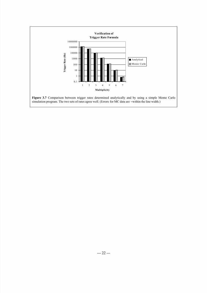
condition. An expression describing this background trigger rate ( f M) for N channels has been
derived in [38]:
4 4 4 4 4 34 4 4 4 4 21
B
M N M
A
M P P M N M
N T M f −−⋅⋅
−⋅= )1(
)!(!! ; P = f dn ⋅ T . (3.6)
Here, “A” is an approximation of 1/T M where T M is the average duration of an accidental M -fold coincidence event, and “B” is the probability to find the detector in an M -fold
coincidence state (due to dark noise) at any given time. The validity of the expression was
verified by a comparison with Monte Carlo simulations of a model detector with its trigger set
at different multiplicity levels. The number of channels in the model detector was N = 100, all
with a dark-noise frequency of f dn = 2 kHz. The result is presented in figure 3.7.
8/3/2019 Pär Lindahl- Energy Calibration of Neutrino Telescopes Using Ultra High Energy Tau Neutrinos
http://slidepdf.com/reader/full/paer-lindahl-energy-calibration-of-neutrino-telescopes-using-ultra-high-energy 27/81
--- 22 ---
Verification of
Trigg er Rate Formula
0,1
1
10
10 0
1000
10000
100000
1000000
1 2 3 4 5 6 7
Multiplicity
T r i g g e r R a t e ( H z )
Analytical
Monte Carlo
Figure 3.7 Comparison between trigger rates determined analytically and by using a simple Monte Carlo
simulation program. The two sets of rates agree well. (Errors for MC data are ∼within the line width.)

8/3/2019 Pär Lindahl- Energy Calibration of Neutrino Telescopes Using Ultra High Energy Tau Neutrinos
http://slidepdf.com/reader/full/paer-lindahl-energy-calibration-of-neutrino-telescopes-using-ultra-high-energy 28/81

8/3/2019 Pär Lindahl- Energy Calibration of Neutrino Telescopes Using Ultra High Energy Tau Neutrinos
http://slidepdf.com/reader/full/paer-lindahl-energy-calibration-of-neutrino-telescopes-using-ultra-high-energy 29/81
--- 24 ---
When an event is initiated electra first determines the time interval to be simulated.
This is defined as starting 5 µs before, and ending 15 µs after the earliest photon hit time. For
this time interval the analog signals from all PMTs are simulated in 1 ns time steps.
For each PMT the simulation starts by generating different signal “features” that will
eventually be combined to form the analog PMT signal. These features include electronic
noise, different pulses from the PMT and cross-talk pulses. After combining all of these the pulse detection is simulated and the trigger conditions are checked. If a trigger is obtained the
ADC (peak amplitude) and TDC (leading and trailing edges) information is extracted. An
outline of the program structure is presented in figure 4.1.
ELECTRA’s Program Structure
DetermineSimulatedTime Interval
ELECTRA
GenerateElectronics
Noise
GeneratePM pulses
Add TimeJitter
GenerateSignalProfile
GenerateDiscriminator Pulses
Check for Trigger
GenerateTDC:s andADC:s
1 Pulse*
1 Pulse*
PulseType
Time atSurface
AmplitudeSimulatePrecesses
Time‘Smearing’
o o
• Direct
• Pre
• Late
• After
• Thermal• Ion
AddPulses
Add Noise
AddCrossTalk
• Simple Majority• - - -
• - - -
Comments
• Sequence: left to right
• Iteration: Indicated *
• Selection: Indicated o
= Not Implemented
Figure 4.1 An outline of electra, a program for simulating the detector electronics in AMANDA.
4.2 An all-channel survey for AMANDA-B13
4.2.1 Introduction
During the austral winter the AMANDA telescope is taking data, and one does not want to
interrupt this process without having strong reasons to do so. Therefore not all details of the
detector can be monitored continuously, and if problems occur during the season they might
elude an early discovery. To be able to take full advantage of the data taken during the year it
is therefore important to perform diagnostic measurements on the detector as soon as the
Amundsen-Scott South Pole Station opens for the summer.
8/3/2019 Pär Lindahl- Energy Calibration of Neutrino Telescopes Using Ultra High Energy Tau Neutrinos
http://slidepdf.com/reader/full/paer-lindahl-energy-calibration-of-neutrino-telescopes-using-ultra-high-energy 30/81
--- 25 ---
For the austral summer of 1999 – 2000 major changes were scheduled for AMANDA.
New strings were to be deployed and the detector electronics were to be upgraded. During one
month in November and December 1999, prior to the scheduled changes, I was responsible
for several investigations performed to be able to describe the status of the electronics in
AMANDA-B13 and to identify problematic detector channels. The main effort was put into
the early stages of the signal chain.
All acquired information is presented in the report [41]. In the following sections some of
the results are presented as a survey over the investigated detector properties.
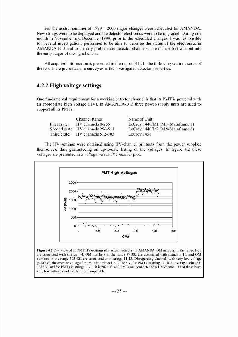
4.2.2 High voltage settings
One fundamental requirement for a working detector channel is that its PMT is powered with
an appropriate high voltage (HV). In AMANDA-B13 three power-supply units are used to
support all its PMTs:
Channel Range Name of UnitFirst crate: HV channels 0-255 LeCroy 1440/M1 (M1=Mainframe 1)
Second crate: HV channels 256-511 LeCroy 1440/M2 (M2=Mainframe 2)
Third crate: HV channels 512-703 LeCroy 1458
The HV settings were obtained using HV-channel printouts from the power supplies
themselves, thus guaranteeing an up-to-date listing of the voltages. In figure 4.2 these
voltages are presented in a voltage versus OM-number plot.
PMT High-Voltages
0
500
1000
1500
2000
2500
0 100 200 300 400 500
OM#
H V [ V o l t ]
Figure 4.2 Overview of all PMT HV-settings (the actual voltages) in AMANDA. OM numbers in the range 1-86are associated with strings 1-4, OM numbers in the range 87-302 are associated with strings 5-10, and OM
numbers in the range 303-428 are associated with strings 11-13. Disregarding channels with very low voltage
(<500 V), the average voltage for PMTs in strings 1-4 is 1685 V, for PMTs in strings 5-10 the average voltage is1635 V, and for PMTs in strings 11-13 it is 2021 V. 419 PMTs are connected to a HV channel. 33 of these have
very low voltages and are therefore inoperable.

8/3/2019 Pär Lindahl- Energy Calibration of Neutrino Telescopes Using Ultra High Energy Tau Neutrinos
http://slidepdf.com/reader/full/paer-lindahl-energy-calibration-of-neutrino-telescopes-using-ultra-high-energy 31/81
--- 26 ---
The result of a closer inspection can be summarized as follows:
• 419 of the PMTs with an OM number in the range 1 – 428 are connected to a HV
channel.
• 33 of these PMTs have very low voltages (<500 V) and are therefore inoperable.
• The average voltage for PMTs in strings 1 - 4 is ∼1685 V (disregarding channels with
very low voltages).
• The average voltage for PMTs in strings 5 - 10 is ∼1635 V (disregarding channelswith very low voltages).
• The average voltage for PMTs in strings 11 - 13 is ∼2021 V (disregarding channels
with very low voltages).
The higher HV setting for strings 11 – 13 will result in a higher gain*. According to [42]
PMTs in strings 1 – 4 (connected to coaxial cables) are operated at a gain of 1.5 ⋅109, PMTs in
strings 4 – 10 (connected to 0.9 mm diameter twisted pair cables) are operated at 0.8 ⋅109
and
PMTs in strings 11 – 13 (connected to 0.7 mm diameter twisted pair cables) are operated at
3.4⋅109. The objective is to drive a 1 photo electron signal over ∼2 km cable, and the different
gain requirements reflect differences in cable and PMT properties. Table 4.1 presents the
batch-dependent HV-settings corresponding to a 1.0 ⋅10
9
gain [42].
Strings HV1 – 4 1618 V
5 – 10 1684 V
11 – 13 1771 V
Table 4.1 Batch-dependent HV-setting corresponding to a 1.0⋅109
gain
Another feature revealed in figure 4.2 is a distribution in the HV settings within each
string. This is explained by individual variations in the PMT properties, and by the fact that
PMTs deployed at greater depths will require a higher gain to overcome the higher attenuation. However, the distribution in PMT properties is used to reduce the differences in
HV settings within a string. Thus, the most “effective” PMTs are deployed at the greatest
depths.
4.2.3 Pulse rates
In the DMADD trigger system, the multiplicity of an event is not obtained in one step.
Instead, first a “local” multiplicity is determined for a subgroup of up to 20 channels,
connected to a so-called MULT20 module. The multiplicities from all subgroups are then
combined in a PREADDER/ADDER sequence to form the “global” multiplicity.
*PMT gain is defined at the number of electrons produced at the anode as a response of a single photo electron.

8/3/2019 Pär Lindahl- Energy Calibration of Neutrino Telescopes Using Ultra High Energy Tau Neutrinos
http://slidepdf.com/reader/full/paer-lindahl-energy-calibration-of-neutrino-telescopes-using-ultra-high-energy 32/81
--- 27 ---
On the front of each MULT20 module it is possible to monitor the discriminated pulses
for channels connected to that module. For each channel in the AMANDA-B trigger system
the following measurements were performed:
• The signal was connected to a scaler where the number of pulses was counted for one
minute, thus determining the pulse rate for that channel.
• The signal was connected to a digital oscilloscope where the pulse width was
measured.• Pulse rate, pulse width and comments about any “strange behavior” were noted.
In figure 4.3 these measurements are presented in a pulse width versus pulse rate plot.
The result of a closer inspection can be summarized as follows:
• 374 channels were connected to the DMADD system.
• 9 channels had very low pulse rates ( f <100 Hz)
• 11 channels had very high pulse rates ( f > 3000 Hz).
• 5 channels were not stable (intermittent signal).
• 46 channels were found to be “silent”, i.e. they showed no signal at their test outputs.
• Typical pulse rates were ∼300 Hz (strings 1 – 4) or ∼1300 Hz (strings 5 - 13).
• Pulse widths were distributed between 2.0 µs and 2.7 µs.
Trigger Input Signals
1,9
2,0
2,1
2,2
2,3
2,4
2,5
2,6
2,7
2,8
1 10 100 1000 10000 100000 1000000
Pulse Rate [Hz]
P u l s e W
i d t h [ m i c r o s e c o n d s ]
Figure 4.3 The discriminated pulses from 374 channels in strings 1 – 13 were used as input to the AMANDA-B
trigger. Both pulse rates and pulse widths were measured at the test outputs on the front of the MULT20
modules. Typical pulse rates were ∼300 Hz (strings 1 – 4) or ∼1300 Hz (strings 5 - 13), and the pulse widths
were distributed between 2.0 µs and 2.7 µs. 46 channels were found to be “silent”, i.e. they showed no signal attheir test outputs.

8/3/2019 Pär Lindahl- Energy Calibration of Neutrino Telescopes Using Ultra High Energy Tau Neutrinos
http://slidepdf.com/reader/full/paer-lindahl-energy-calibration-of-neutrino-telescopes-using-ultra-high-energy 33/81
--- 28 ---
A large fraction of the PMT background pulse rates is believed to be due to exposure
from radioactive material in the spherical glass vessels that are used for housing the PMTs.
Measurements of the content of different radionuclides in the glass is presented in the report
[43]. The type of vessel used in strings 5 – 13 (BENTHOS) was found to contain significant
amounts of uranium, thorium and potassium (U, Th, K). The type of vessel used in strings 1 –
4 (BILLINGS) was found to contain similar amounts of U and Th but only about 4% as much
K compared with the BENTHOS spheres. It is therefore believed that the difference in theamount of K in the two types of glass vessels is the probable cause for the observed difference
in pulse rates (see figure 4.3).
In [42] the pulse rates are used together with the corresponding HV settings to calculate
the amount of charge leaving the anode of PMTs in different strings. The annual anode
charges thus obtained are 0.9 C for strings 1 – 4, 1.6 C for strings 5 – 10 and 7 C for strings
11 – 13. These numbers are important since the lifetime of a PMT is limited by the total
integrated charge. For the PMTs used in AMANDA a 50% gain drop (at constant HV) is
expected for an integrated charge of ∼115 C [42].
4.2.4 Pulse shapes
One important “tool” for diagnosing the operation of a SWAMP (and the PMT connected to
it) is to look for any strange features in the shape of its PMT pulses. With the experience from
looking at many signals I formed a subjective opinion about what “normal” pulses should
look like. A few channels with pulses falling into this category were selected. For each
channel a number of pulses were digitized at the prompt line (using a 500 MHz digital
oscilloscope) to be used as reference pulses.
In figure 4.4, a selection of the digitized pulses is presented. In these plots a couple of
pulse-shape features may be noted, which appear in a systematic manner: First, as expected,
the pulse widths are larger for PMTs deployed at greater depths, since these channels are
equipped with longer cables. Secondly, in strings 11 – 13 we observe a clear difference
between the pulse shapes from odd numbered PMTs (position number in the string) compared
with even numbered ones. In the “odd” case one sees a “kink” on the trailing edge of all
pulses, which is not observed for “even” channels. The cause of this effect has not been
determined, but one suggestion is that it is due to signal reflections in the connector for the
“pigtail” connecting every odd-numbered OM to the cable near its position in the hole.
In addition, when comparing pulses, one should be aware of that due to development over
the years different cables as well as different versions of SWAMPs have been used. In
November 1999 three “generations” of cable/SWAMP combinations were used, with slightly
different pulse shapes. The three generations are defined as:
• Generation 1: Strings 1 – 4 (OMs 1-86)
• Generation 2: Strings 5 – 10 (OMs 87-302)
• Generation 3: Strings 11 – 13 (OMs 303-428)
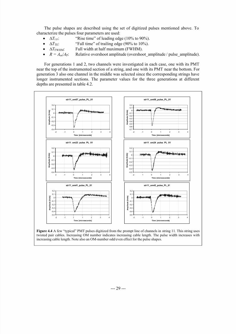
8/3/2019 Pär Lindahl- Energy Calibration of Neutrino Telescopes Using Ultra High Energy Tau Neutrinos
http://slidepdf.com/reader/full/paer-lindahl-energy-calibration-of-neutrino-telescopes-using-ultra-high-energy 34/81
--- 29 ---
The pulse shapes are described using the set of digitized pulses mentioned above. To
characterize the pulses four parameters are used:
• ∆T LE: “Rise time” of leading edge (10% to 90%).
• ∆T TE: “Fall time” of trailing edge (90% to 10%).
• ∆T FWHM: Full width at half maximum (FWHM).
• R = Aos/ AP: Relative overshoot amplitude (overshoot_amplitude / pulse_amplitude).
For generations 1 and 2, two channels were investigated in each case, one with its PMT
near the top of the instrumented section of a string, and one with its PMT near the bottom. For
generation 3 also one channel in the middle was selected since the corresponding strings have
longer instrumented sections. The parameter values for the three generations at different
depths are presented in table 4.2.
str11_om07_pulse_PL_01
-0,4
-0,3
-0,2
-0,1
0
0,1
0,2
-2 -1 0 1 2 3 4
Time [microseconds]
A m p l i t u d e [ V o l t s ]
str11_om08_pulse_PL_01
-0,7
-0,6
-0,5
-0,4
-0,3
-0,2
-0,1
0
0,1
0,2
-2 -1 0 1 2 3 4
Time [microseconds]
A m p l i t u d e [ V o l t s ]
str11_om23_pulse_PL_01
-0,4
-0,3
-0,2
-0,1
0
0,1
0,2
-2 -1 0 1 2 3 4Time [microseconds]
A m p l i t u d e [ V o l t s ]
str11_om24_pulse_PL_01
-0,5
-0,4
-0,3
-0,2
-0,1
0
0,1
0,2
-2 -1 0 1 2 3 4Time [microseconds]
A m p l i t u d e [ V o l t s ]
str11_om41_pulse_PL_01
-0,5
-0,4
-0,3
-0,2
-0,1
0
0,1
0,2
-2 -1 0 1 2 3 4
Time [microseconds]
A m p l i t u d e [ V o l t s ]
str11_om42_pulse_PL_01
-0,5
-0,4
-0,3
-0,2
-0,1
0
0,1
0,2
-2 -1 0 1 2 3 4
Time [microseconds]
A m p l i t u d e [ V o l t s ]
Figure 4.4 A few “typical” PMT pulses digitized from the prompt line of channels in string 11. This string uses
twisted pair cables. Increasing OM number indicates increasing cable length. The pulse width increases withincreasing cable length. Note also an OM-number odd/even effect for the pulse shapes.
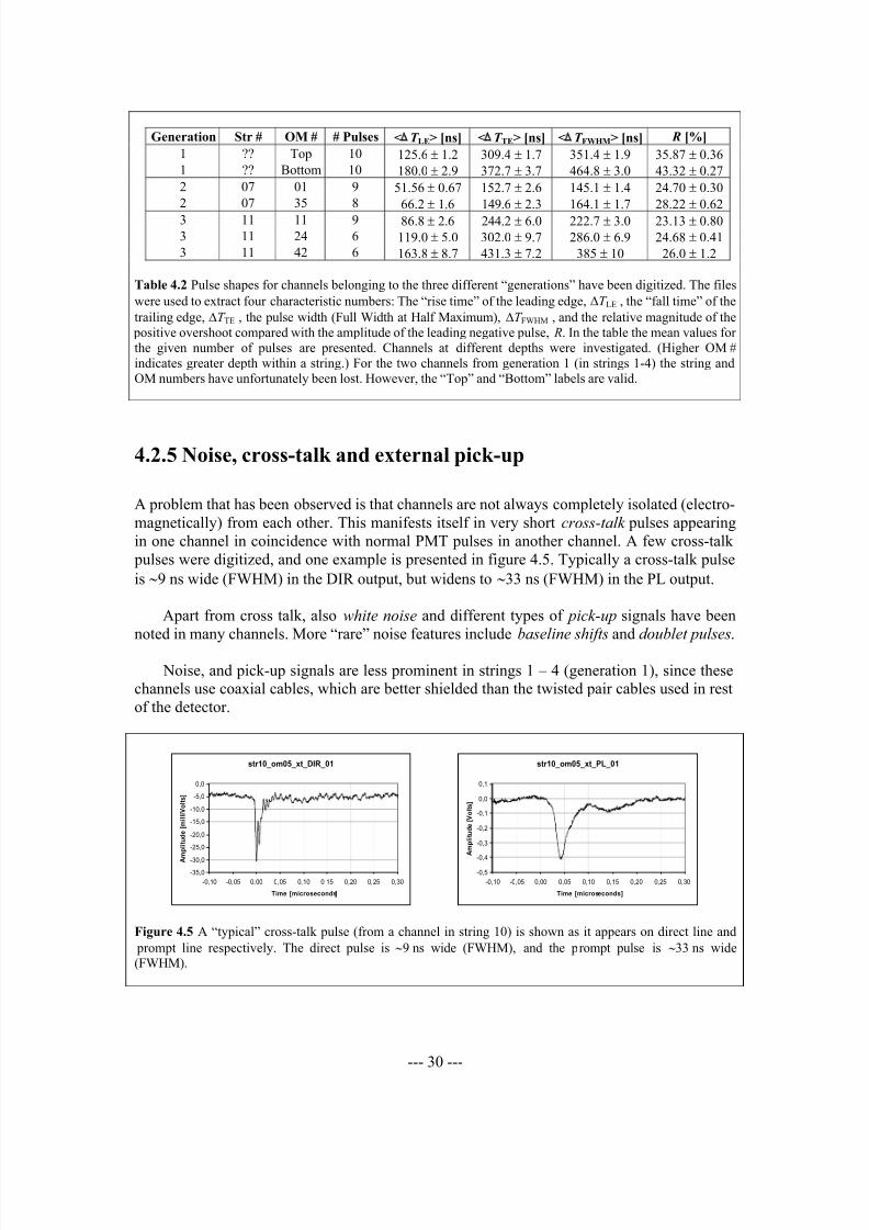
8/3/2019 Pär Lindahl- Energy Calibration of Neutrino Telescopes Using Ultra High Energy Tau Neutrinos
http://slidepdf.com/reader/full/paer-lindahl-energy-calibration-of-neutrino-telescopes-using-ultra-high-energy 35/81
--- 30 ---
Generation Str # OM # # Pulses <∆T LE> [ns] <∆T TE> [ns] <∆T FWHM> [ns] R [%]
1 ?? Top 10 125.6 ± 1.2 309.4 ± 1.7 351.4 ± 1.9 35.87 ± 0.36
1 ?? Bottom 10 180.0 ± 2.9 372.7 ± 3.7 464.8 ± 3.0 43.32 ± 0.27
2 07 01 9 51.56 ± 0.67 152.7 ± 2.6 145.1 ± 1.4 24.70 ± 0.30
2 07 35 8 66.2 ± 1.6 149.6 ± 2.3 164.1 ± 1.7 28.22 ± 0.62
3 11 11 9 86.8 ± 2.6 244.2 ± 6.0 222.7 ± 3.0 23.13 ± 0.803 11 24 6 119.0 ± 5.0 302.0 ± 9.7 286.0 ± 6.9 24.68 ± 0.413 11 42 6 163.8 ± 8.7 431.3 ± 7.2 385 ± 10 26.0 ± 1.2
Table 4.2 Pulse shapes for channels belonging to the three different “generations” have been digitized. The files
were used to extract four characteristic numbers: The “rise time” of the leading edge, ∆T LE , the “fall time” of the
trailing edge, ∆T TE , the pulse width (Full Width at Half Maximum), ∆T FWHM , and the relative magnitude of the
positive overshoot compared with the amplitude of the leading negative pulse, R. In the table the mean values for
the given number of pulses are presented. Channels at different depths were investigated. (Higher OM #
indicates greater depth within a string.) For the two channels from generation 1 (in strings 1-4) the string and
OM numbers have unfortunately been lost. However, the “Top” and “Bottom” labels are valid.
4.2.5 Noise, cross-talk and external pick-up
A problem that has been observed is that channels are not always completely isolated (electro-
magnetically) from each other. This manifests itself in very short cross-talk pulses appearing
in one channel in coincidence with normal PMT pulses in another channel. A few cross-talk
pulses were digitized, and one example is presented in figure 4.5. Typically a cross-talk pulse
is ∼9 ns wide (FWHM) in the DIR output, but widens to ∼33 ns (FWHM) in the PL output.
Apart from cross talk, also white noise and different types of pick-up signals have been
noted in many channels. More “rare” noise features include baseline shifts and doublet pulses.
Noise, and pick-up signals are less prominent in strings 1 – 4 (generation 1), since these
channels use coaxial cables, which are better shielded than the twisted pair cables used in rest
of the detector.
str10_om05_xt_DIR_01
-35,0
-30,0
-25,0
-20,0
-15,0
-10,0
-5,0
0,0
-0,10 -0,05 0,00 0,05 0,10 0,15 0,20 0,25 0,30
Time [microseconds]
A
m p l i t u d e [ m i l l i V o l t s ]
str10_om05_xt_PL_01
-0,5
-0,4
-0,3
-0,2
-0,1
0,0
0,1
-0,10 -0,05 0,00 0,05 0,10 0,15 0,20 0,25 0,30
Time [microseconds]
A m p l i t u d e [ V o l t s ]
Figure 4.5 A “typical” cross-talk pulse (from a channel in string 10) is shown as it appears on direct line and
prompt line respectively. The direct pulse is ∼9 ns wide (FWHM), and the prompt pulse is ∼33 ns wide(FWHM).

8/3/2019 Pär Lindahl- Energy Calibration of Neutrino Telescopes Using Ultra High Energy Tau Neutrinos
http://slidepdf.com/reader/full/paer-lindahl-energy-calibration-of-neutrino-telescopes-using-ultra-high-energy 36/81
--- 31 ---
4.2.6 SWAMP gain and delay
The amplitude gains in PL and DEL outputs, and the delay between PL and DEL outputs were
measured for all operational SWAMPs. In order to do so the following set-up was assembled:
A pulse generator was used to produce test-pulses with a shape similar to PMT-pulses as theyappear in the DIR output. The pulse shape (after attenuation) was measured with a digital
oscilloscope to have the following characteristics (negative pulses):
DC Offset: 2 mV
Leading Edge Fall-Time: 100 ns
Trailing Edge Rise-Time: 186 ns
Width (FWHM): 220 ns
Amplitude: 12.6 mV
This signal was connected to a lemo-T thus splitting the signal to the oscilloscope (1 M Ω
termination) and the Direct Line of the SWAMP, which was now used as an injection point.
The Prompt and Delayed outputs from the SWAMP were connected to two other inputs on the
oscilloscope (50 Ω termination).
For each SWAMP the amplitudes of the injected signal, ATST, the prompt signal, APL, and
the Delayed signal, ADEL, were measured. The PL-gain was defined as GPL = APL/ ATST, and the
DEL-gain was defined as GDEL = ADEL/ ATST. (Note the fundamental difference between these
gain definitions and the PMT gain, which specify the number of electrons leaving the anode
for each initial photo electron.) The SWAMP-delay ∆T was measured between the starting
points*
of the pulses in PL and DEL.
These measurements (PL-gain, DEL-gain and SWAMP-delay) yield the status of the
SWAMP performance, without depending on the presence of “good looking” PMT pulses.
The measurements are presented in two plots: Figure 4.6 shows GDEL versus GPL, and
figure 4.7 shows the ∆T distribution.
* The starting point of a pulse was found by eye extrapolating the leading-edge slope back to the point where it
would cross the signal base line.

8/3/2019 Pär Lindahl- Energy Calibration of Neutrino Telescopes Using Ultra High Energy Tau Neutrinos
http://slidepdf.com/reader/full/paer-lindahl-energy-calibration-of-neutrino-telescopes-using-ultra-high-energy 37/81
--- 32 ---
SWAMP Gains
0
50
100
0 50 100 150 200 250
Gain (PL)
G a i n ( D E L )
Figure 4.6 Two versions of the amplified PMT signal are available on different SWAMP outputs. The prompt
signal is used for extracting time information and for trigger purposes. The delayed signal is used for extractingamplitude information. Presented here is the gain distribution for the two outputs (delayed vs. prompt). Typical
gains were [GPL≈60, GDEL≈10] (strings 1 – 4) or [GPL≈80, GDEL≈35] (strings 5 – 13). The total number of SWAMPs was 442. 35 of these were found to be “dead”, i.e. they showed no signals at the amplified outputs.
One was “semi-dead”, with signal in prompt but not in delayed output.
The result of a closer inspection can be summarized as follows:
• The total number of SWAMPs was 442
• One SWAMP showed two almost identical pulses in the DEL output. (The first pulse
was in coincidence with the pulse in the PL output; the second had a “normal” delay.)
• One SWAMP showed signal in PL but not in DEL.
•
35 SWAMPs were found to be “dead”, i.e. they showed no signals in PL and DEL.• Typical gains were [GPL≈60, GDEL≈10] (strings 1 – 4) or [GPL≈80, GDEL≈35] (strings
5 – 13).
• Almost all SWAMPs had a delay somewhere between 2.00 µs and 2.17 µs. (One
channel singled out with a delay of 1.05 µs.) The average delay was 2.09 µs.

8/3/2019 Pär Lindahl- Energy Calibration of Neutrino Telescopes Using Ultra High Energy Tau Neutrinos
http://slidepdf.com/reader/full/paer-lindahl-energy-calibration-of-neutrino-telescopes-using-ultra-high-energy 38/81
--- 33 ---
SWAMP Delay
6
14
58
17 1711 11
31
40
54
76
46
38
17
10
1 3
0
10
20
30
40
50
60
70
80
2 ,
0 0
2 ,
0 1
2 ,
0 2
2 ,
0 3
2 ,
0 4
2 ,
0 5
2 ,
0 6
2 ,
0 7
2 ,
0 8
2 ,
0 9
2 ,
1 0
2 ,
1 1
2 ,
1 2
2 ,
1 3
2 ,
1 4
2 ,
1 5
2 ,
1 6
2 ,
1 7
Time (microseconds)
# S W A M P s
Figure 4.7 Two versions of the PMT signal are available on different SWAMP outputs. The prompt signal is
used for extracting time information and for trigger purposes. The delayed signal is used for extracting amplitudeinformation. Here is the distribution of delay times between these two outputs. (Note: One SWAMP with a delayof 1.05 µs is “out of scale” in this plot.) The total number of SWAMPs was 442. 35 of these were found to be
“dead”, i.e. they showed no signals at the amplified outputs. One was “semi-dead”, with signal in prompt but notin delayed output. The mean delay was 2.09 µs.

8/3/2019 Pär Lindahl- Energy Calibration of Neutrino Telescopes Using Ultra High Energy Tau Neutrinos
http://slidepdf.com/reader/full/paer-lindahl-energy-calibration-of-neutrino-telescopes-using-ultra-high-energy 39/81
--- 34 ---
Chapter 5
Cascade-like events
5.1 Intrinsic cascade properties
5.1.1 General properties
In the experimental data from AMANDA two types of event signatures may be identified
using present day algorithms, tracks and cascades. The physical origin of the track signature
is events where a charged particle propagates through a substantial part of the detector at a
relativistic speed, while emitting Čerenkov radiation (see section 3.1). The origin of the
cascade signature is events where an initial particle gives rise to extensive particle production
at essentially a single point within or in the vicinity of the detector. These cascade events are
initiated either when the initial particle reacts with the detector medium (ice) or when the particle decays in flight.
In chapter 10 a method is outlined for energy calibration of neutrino telescopes with
respect to cascade events. Relevant cascade properties in this context are e.g. the geometry of
these events, in particular their longitudinal development, and the amount of photons
produced.
It should be noted that cascades are not exactly pointlike but do have a longitudinal
extension - a length - in the direction of the velocity of the initial particle. This length is
essentially proportional to the logarithm of the energy. Thus, the assumption that cascades are
point-like is only valid if the energy deposit is not too high. Typical cascade lengths in water
for cascades of a few PeV (representative for the events at focus in this thesis) lie between10 m and 20 m [44] [45]. (The corresponding lengths in ice are obtained by multiplying by
the density ratio ρ water / ρ ice.) After this distance only a small fraction of the initial energy
remains to be deposited. These lengths are comparable to the distances between optical
modules both in AMANDA-II and in IceCube (see section 3.1). Since the present
reconstruction algorithms for cascade events assume that cascades are point-like it is possible
that these algorithms will have to be modified to be able to support reconstruction of ultra-
high energy cascades.

8/3/2019 Pär Lindahl- Energy Calibration of Neutrino Telescopes Using Ultra High Energy Tau Neutrinos
http://slidepdf.com/reader/full/paer-lindahl-energy-calibration-of-neutrino-telescopes-using-ultra-high-energy 40/81
--- 35 ---
In calorimetric measurements of cascade events the signal amplitude obtained through the
detection/analysis process should ideally be proportional to the number of photons produced.
(Insufficient sampling in space will introduce a component of statistical uncertainty.) On
average the number of photons produced in a cascade is proportional to the energy deposit,
but since the particle production in cascades is a stochastic process there will, in general, be
statistical fluctuations in the event-to-event number of photons per unit energy [45].
Furthermore, since the amount of photons produced per unit energy depends on the
nature of the initial particle, the particle type (or at least the a priori probabilities for different
particle types) should be known to enable the calculation of the energy deposit in a cascade
event.
5.1.2 Electromagnetic cascades
The initiators for electromagnetic cascades are electrons and photons, but neutral pions may
also be placed in this group of initiators due to their “prompt” decay into two photons.
There are two main processes that govern the development of an electromagnetic cascade,
the production of a bremsstrahlung photon when an electron or a positron is accelerated in the
field of a nucleus, and the conversion of a photon into an electron-positron pair. The result of
these alternating processes is an “avalanche” of increasing numbers of electrons/positrons and
photons. However, for each new “generation” the energy of the “daughter” particles will be
lower than the energy of the “parent” particle. Eventually the electron energies will begin
falling below a certain critical energy. The particle production stops and the cascade dies out
[18].
Along the longitudinal development of the cascade electrons and positrons will emit
Čerenkov photons. The number of photons will be roughly proportional to the total track-
length of all charged particles participating in the cascade. For electromagnetic cascades the
event-to-event fluctuations in the number of photons produced for a given energy E of the
initiator particle is very small. GEANT [46]-based simulations performed for the BAIKAL
experiment [44] have shown that the total track-length for an electromagnetic cascade in
water is approximately
( ) ( ) 89.4GeV1/ ⋅= E E L m (5.1)
For the wavelength interval where the PMTs are sensitive (300-600 nm) the photon yield in
ice is ∼3.30⋅104
photons/m track [30], but since the number of Čerenkov photons for non-
relativistic particles is smaller, the average yield is reduced. For electromagnetic cascades in
water this correction factor was found to be 0.894 [44]. Thus, neglecting the difference in
density between the detector medium at the BAIKAL and AMANDA/IceCube sites, electro-
magnetic cascades are expected to produce ∼1.44⋅105 (detectable) Čerenkov photons per GeV.

8/3/2019 Pär Lindahl- Energy Calibration of Neutrino Telescopes Using Ultra High Energy Tau Neutrinos
http://slidepdf.com/reader/full/paer-lindahl-energy-calibration-of-neutrino-telescopes-using-ultra-high-energy 41/81
--- 36 ---
5.1.3 Hadronic cascades
With hadronic initiators the development of the cascades is more complex than in electro-
magnetic cascades, but since the basic interactions are well understood the particle production
may be studied using Monte Carlo simulations.
As the cascade develops, secondary (charged) particles will emit Čerenkov radiation.
There are, however, a couple of differences between hadronic and electromagnetic cascades
that must be considered. On average hadronic cascades produce less amounts of photons
compared with electromagnetic cascades, and the event-to-event fluctuations are larger, given
the same incident energy.
The reason for the lower average number of photons is that energy is lost to low-energy
neutrons and to the breaking of nuclei (binding energy). The reason for the larger fluctuations
is that neutral pions amount, on average, to one third of the produced pions, and the energy
carried by these neutral particles is deposited as electromagnetic cascades with a higher
photon yield. The number of produced neutral pions early in the development of the cascadewill therefore have a large impact on the total number of photons produced.
The GEANT-based simulations for the BAIKAL experiment [44] have shown that, on
average, the total track-length for a hadronic cascade is approximately
( ) ( ) 08.4GeV1/ ⋅= E E L m. (5.2)
The photon yield is ∼3.30⋅104
photons/m track [30] times a correction factor of 0.86 [44].
Thus, if the difference in density between the detector medium at the BAIKAL and
AMANDA/IceCube sites is neglected, hadronic cascades are expected to produce ∼1.16⋅105
Čerenkov photons per GeV (average value). This is about 80% of the photon yield in electro-
magnetic cascades.
5.2 Cascade detection
5.2.1 Introduction
Two reconstruction methods for cascades have been developed for the AMANDA-B10
detector [47], where cascades are regarded as point-like bursts of light with very short
duration. A mathematical model is used for describing the emission, absorption and scattering
of Čerenkov photons. The directions of the emitted photons are peaked at the Čerenkov angle
with respect to the direction of the velocity of the cascade initiator particle.

8/3/2019 Pär Lindahl- Energy Calibration of Neutrino Telescopes Using Ultra High Energy Tau Neutrinos
http://slidepdf.com/reader/full/paer-lindahl-energy-calibration-of-neutrino-telescopes-using-ultra-high-energy 42/81
--- 37 ---
5.2.2 Reconstruction of position and time
The first reconstruction method is used for determining the position and time of a cascade
event. From the Čerenkov model a probability distribution ( )d t p ,del is derived for the
expected “time delay” ( delt ) between the observed photon hit time on an OM – at a distance d from the cascade – and the expected hit time without scattering:
iceeventhitdel / cd t t t −−= (5.3)
A likelihood function is then constructed for all observed hit-times in an event
( )∏=
=hits
0
del, N
i
i
i d t pL , (5.4)
and the cascade parameters (position and time) are varied until the values corresponding to
the maximum likelihood have been found.
5.2.3 Reconstruction of energy and direction
The second reconstruction method is used to obtain the energy and direction of a cascade. It
uses the following expressions for the probabilities for a given OM to observe or not observe
a signal from Čerenkov photons:η −−= e P 1hit (5.5a)
η −= e P no_hit (5.5b)
The number of photons (η ) hitting an OM is proportional to the energy of the cascade [44],
and also depends on the cascade direction and the vector that joins the cascade vertex and the
OM. A functional form of η has been determined, thus making it possible to construct the
likelihood function
∏ ∏×=hit_OMs no_hit_OMs
no_hithit P P L . (5.6)
Since the position of the cascade vertex may be determined by the reconstruction method
described in section 5.2.2 the energy and direction of the cascade are the only remaining free
parameters in (5.6). These parameters are varied until the values corresponding to the
maximum likelihood have been found.
5.2.4 Reconstruction performance
To extract cascade-event candidates each event detected with AMANDA is submitted to a
selection algorithm, which selects events with certain properties presumed to be characteristic
for cascade events. In [47] an investigation of the performance of these reconstruction
methods is presented for the AMANDA-B10 detector (including simulation, selection and
reconstruction of cascades). It shows that the expected energy resolution is ∼45% in (log10 E ν -
log10 E C) in the range 3 TeV < E ν < 10 TeV, Here, E ν denotes the true energy of an electronneutrino initiating the cascade, and E C denotes the reconstructed cascade energy.

8/3/2019 Pär Lindahl- Energy Calibration of Neutrino Telescopes Using Ultra High Energy Tau Neutrinos
http://slidepdf.com/reader/full/paer-lindahl-energy-calibration-of-neutrino-telescopes-using-ultra-high-energy 43/81
--- 38 ---
The investigation also shows that the expected position resolutions differ between
coordinates in the horizontal plane ( x and y) and the vertical coordinate ( z ): The r.m.s. values
for the error distributions in reconstructed coordinates are 17.8 m for the x and y coordinates
and 7.1 m in the z coordinate.
In a later paper [48] a similar investigation was done for AMANDA-II. For simulated
mono energetic cascades ( TeV100TeV1.0 ≤≤ ν E ), distributed within the detector, the position resolution was in the order of 5 m. The energy resolution was 0.1 – 0.2 in
log10( E C/1PeV).
In chapter 10 an energy calibration method for cascades is described using so-called
double bang events (see section 6.1), where two cascades are produced within the detector
volume. The potential for this method relies on the possibility to reconstruct the position (and
time) of both of these cascades, and the energy of one of them. Since no attempt has been
made to design a reconstruction algorithm for these events the performance of the single-
cascade reconstruction in AMANDA-II will be used as an example of what might be possible
to obtain for cascades in double bang events in the future.

8/3/2019 Pär Lindahl- Energy Calibration of Neutrino Telescopes Using Ultra High Energy Tau Neutrinos
http://slidepdf.com/reader/full/paer-lindahl-energy-calibration-of-neutrino-telescopes-using-ultra-high-energy 44/81
--- 39 ---
Chapter 6
Detection of tau neutrinos
6.1 The double bang signature
6.1.1 Overview
One characteristic signature for tau neutrino reactions that might be observed in neutrino
telescopes, like AMANDA or IceCube, is the so-called double bang signature: two large
cascades separated in space and time by a tauon traveling close to the speed of light.
This signature occurs in a subset of the possible reaction schemes between a tau neutrino
and a nucleon. The first “bang” is the hadronic cascade produced in a charged current reaction
between the neutrino and a nucleon in the target material (ice). From this reaction a tauonemerges, emitting Čerenkov radiation as it propagates through the material. Eventually, the
tauon decays and, depending on the nature of its daughters, a second cascade (the second
bang) might occur, thus finalizing the signature (see figure 6.1).
ντ
τ
1st cascade
2nd cascade
Figure 6.1 The double bang signature — two large cascades separated in space and time by a relativistic
tauon — is a characteristic signature for a tau neutrino interacting with a nucleon.

8/3/2019 Pär Lindahl- Energy Calibration of Neutrino Telescopes Using Ultra High Energy Tau Neutrinos
http://slidepdf.com/reader/full/paer-lindahl-energy-calibration-of-neutrino-telescopes-using-ultra-high-energy 45/81
--- 40 ---
The detection of double bang events in large neutrino telescopes is discussed in [7]. It is
suggested that due to their unique signature there will probably be almost no background to
these events. In this context, the word “background” refers to events that can fake the double
bang signature. The most serious background contribution will, according to [7], be muon
neutrino charged current events where the muon travels approximately 100 m before loosing
most of its energy in a single bremsstrahlung reaction.
The fraction of muon neutrino charge current events having a signature similar to this is
expected to be of the order 3103 −⋅ . In section 9.5 this number will be used to estimate the
signal-to-background ratio in the AMANDA-II and IceCube detectors due to these
background events.
6.1.2 The neutrino-nucleon reaction
Tau neutrinos ( τ ν ) interact with nucleons (the isoscalar nucleon:2
n p N
+= ) through one of
the following weak-interaction schemes:
• Charged current (CC) reaction: ""CC anything τ N ντ + → +
• Neutral current (NC) reaction: "" NC anything ν N ν τ τ + → +
For both of these, energy is transferred to the struck quark of the target nucleon causing the
nucleon to break. The result is a hadronic cascade. The fraction of the neutrino energy that is
transferred to the quark is called the inelasticity of the reaction and is denoted by y. For the
charged current reaction
ν
τ
E
E y −= 1 (6.1a)
where E ν is the energy of the incident neutrino and E τ is the energy of the tauon produced in
the reaction. For the neutral current reaction
ν
ν
E
E y
′−= 1 (6.1b)
where ν E ′ is the energy of the neutrino escaping from the reaction vertex.
The cross sections for these two reaction schemes depend on the internal structure (quark
content) of the nucleon. Each nucleon consists of three so-called “valence quarks”
determining the electric charge ( proton: uud ⇒ Q p = +1e. neutron:udd ⇒ Qn = 0), but in
addition virtual quark/anti quark pairs are produced and annihilated continuously “inside” the
nucleon. These virtual quarks are called “sea-quarks”, and are available for reactions with e.g.
neutrinos. The quark content may be described in terms of the so-called parton distributions,
)( xq f . The Bjorken scaling variable x is the fraction of the four-momentum of the nucleoncarried by a single parton (quark). Thus x xq f d)( is the expectation value of the number of
quarks of flavor f in the nucleon whose four-momentum lies in the interval [ x, x+d x]. The
corresponding parton distributions for antiquarks are denoted by )( xq f .

8/3/2019 Pär Lindahl- Energy Calibration of Neutrino Telescopes Using Ultra High Energy Tau Neutrinos
http://slidepdf.com/reader/full/paer-lindahl-energy-calibration-of-neutrino-telescopes-using-ultra-high-energy 46/81
--- 41 ---
The parton distributions are not known from first principles but have to be determined
from experiments. In high-energy reactions the small- x quarks makes an important
contribution to the cross-section. However, the small- x region has not been completely
“mapped out” yet. Instead when trying to estimate the cross-sections for these reactions one
has to rely on extrapolations of parameterized models of the parton distributions. One modern
set of models for parton distributions is named CTEQ4-DIS [49]. The calculated cross
sections for deeply inelastic neutrino-nucleon scattering (at neutrino energies between 109
eVand 10
21eV) using these distributions are presented in [22].
6.1.3 The tauon propagation
A tauon has a very short mean lifetime [18]
t τ = (290.6 ± 1.1) ⋅ 10-15
s. (i)This corresponds to a mean range of only
ct τ = (87.12 ± 0.33) ⋅ 10-6
m (ii) for a particle traveling close to the speed of light. However, for the most energetic neutrino
reactions the emerging tauons will be extremely relativistic, and due to time dilation the
observed mean range ( R) in the lab frame is proportional to the gamma factor (γ ):
τ τ
τ τ ct cm
E ct E R ⋅=⋅=
2)(
τ
γ , (6.2)
where the tauon rest mass is [18]30.0
26.003.1777+−=τ m MeV/c2
. (iii)
By inserting (ii) and (iii) into equation (6.2) one obtains a simple expression that will be
used in the following chapters:
⋅≈
GeV1
µm49)( τ τ
E E R (6.2’)
Thus, for tauon energies in the order of 1 PeV or higher the tauon mean ranges will be tens or
hundreds of meters. The decay follows an exponential distribution, so the distribution in
ranges (r ) will also be exponential with a mean range according to equation (6.2’):
-r/R
Rr f e
1)( = ; 0≥r (6.3)
As the tauon propagates through the detector medium it will loose energy, and one might
ask how this will influence the tauon range. To determine this one needs to consider the
energy loss per unit length. Two types of losses must be considered, ionization losses – which
are high at low energies, drop to a minimum and then increase slowly with energy – and
radiation losses – which are essentially proportional to the tauon energy at high energies. Athigh tauon energies ( τ E ) the losses per unit length may therefore be approximated by a linear
equation
τ τ τ E ba x
E τ ⋅+≈−d
d(6.4)
where τ a is due to ionization losses and τ b is due to radiation losses. Both τ a and τ b are
slowly varying functions with energy, but according to [50] the asymptotic values for these
functions at high energies are

8/3/2019 Pär Lindahl- Energy Calibration of Neutrino Telescopes Using Ultra High Energy Tau Neutrinos
http://slidepdf.com/reader/full/paer-lindahl-energy-calibration-of-neutrino-telescopes-using-ultra-high-energy 47/81
--- 42 ---
⋅⋅≈
⋅⋅≈
− 1-
water
ice6
1-
water
ice
m 1078.1
mGeV 2.0
ρ
ρ
ρ
ρ
τ b
aτ
(6.5)
Assuming the approximate value 92.0water ice ≈ ρ ρ for the relative density of ice at ∼1 atm
and temperatures close to 0 °C, one gets the result,
⋅≈
⋅≈− 1-6
-1
m 106.1
mGeV 2.0
τ
τ
b
a(6.5’)
For a tauon with energy 1 PeV the mean range is ∼50 m, and according to equations (6.4)
and (6.5’) it will loose ∼2 GeV/m. This implies that only ∼0.01% of its initial energy will be
lost. For a 10 PeV tauon ∼0.1% of the initial energy will be lost. The influence on the tauon
range may therefore be neglected at these energies.
It is interesting to make a comparison with the muon energy losses. According to [50] theenergy loss per unit length is roughly proportional to the inverse of the mass squared for the
propagating particle. For a muon ( µ )
µ µ µ
µ E ba
x
E ⋅+≈−
d
d, (6.6)
where (for ice)
⋅≈⋅≈
⋅≈≈− 1-4
-1
m 106.3219
mGeV 2.0
τ µ
τ µ
bb
aa. (6.7)
A 1 PeV muon will thus loose almost 200 times more energy per unit length compared with a
tauon of the same energy.
6.1.4 The tauon decay
The tauon decay is described by
""anything ντ τ +→ ,
where “anything ” stands for either hadrons — probability ∼65% — or leptons — eνe + :
probability ∼18% or µν µ + : probability ∼17% — [18]. If the decay follows either the
hadronic channel or the leptonic channel to an electron and an electron neutrino, there will be
a second “bang” completing the double-bang signature (two separate cascades). If the decay
follows the leptonic channel to a muon and a muon neutrino, there will not be a second bang.Instead the emerging muon will continue the tauon track (possibly with small change in
direction), emitting Čerenkov radiation.
8/3/2019 Pär Lindahl- Energy Calibration of Neutrino Telescopes Using Ultra High Energy Tau Neutrinos
http://slidepdf.com/reader/full/paer-lindahl-energy-calibration-of-neutrino-telescopes-using-ultra-high-energy 48/81
--- 43 ---
6.2 Detection criteria
In chapter 9 an attempt is made to estimate the expected double bang event rates. For this
purpose it is necessary to characterize the limitations of the detector. Following the discussion
in [7] regarding the energy threshold for the detection of double bang events it is suggestedthat at least three detection criteria must be fulfilled:
1) For the double bang events to be detected it is essential that all three parts of the signature
(the two cascades and the connecting tauon track) are sampled. It is reasonable to believe
that this can only be done if the event is completely contained within the detector.
2) To be able to distinguish the two cascades from each other they must be sufficiently well
separated. This minimum separation (r min) will depend on the density and distribution of
optical modules within the detector.
3) For a cascade to be recognized as such it must be very bright. Both cascades of a double
bang event must therefore individually produce photons in numbers corresponding to an
electromagnetic cascade exceeding some minimal energy ( E min).
These criteria will be used in section chapter 9.3 to develop a parameterized model for
the “effective volume” (V eff ) of a generic detector, and to determine the V eff values for the
AMANDA-II and IceCube detectors (using the detector simulation routines described in
section 7.3).

8/3/2019 Pär Lindahl- Energy Calibration of Neutrino Telescopes Using Ultra High Energy Tau Neutrinos
http://slidepdf.com/reader/full/paer-lindahl-energy-calibration-of-neutrino-telescopes-using-ultra-high-energy 49/81
--- 44 ---
Chapter 7
Simulation- and analysis tools
7.1 Overview
To be able to study the properties of double bang events — described in chapter 6 — a
number of FORTRAN programs were developed:
• for “generating” neutrinos and simulating the subsequent reactions (gen_nutau),
• for identifying events with the “double bang signature” and extracting relevant event
information (ana_db),
• for simulating the detector response (db_det), and
• for analyzing the correlation between tauon range and visible energy produced when
the tauon decays (corr_RE and histo_RE).
The order in which to use these programs is illustrated in figure 7.1.
Detect ?
gen_nutau
ana_db
db_det
corr_RE
histo_RE
Y
Figure 7.1 Illustration of the order in which to use the different simulation- and analysis tools for analyzing
double bang events.

8/3/2019 Pär Lindahl- Energy Calibration of Neutrino Telescopes Using Ultra High Energy Tau Neutrinos
http://slidepdf.com/reader/full/paer-lindahl-energy-calibration-of-neutrino-telescopes-using-ultra-high-energy 50/81
--- 45 ---
7.2 Event generator
To be able to study tau neutrino reactions with nucleons a generator program “gen_nutau”
(written in FORTRAN 77) was developed. The FORTRAN routines in PYTHIA ver. 6.157
[51] were used for simulation of all primary particle reactions and for the particle production
associated with tauon decay.
The program generates tau neutrinos with their momentum directed along the positive z -axis and with energies picked from a power-law spectrum specified by the user by giving the
spectral index α according to equation 2.3. (Typical value: α = 2. See section 2.2.3.) These
neutrinos are made to react with either a proton or a neutron picked at random for each event.
The probabilities for the two nucleon-types are preset to reflect the nucleon content of water.
Thus, proton targets are selected with a probability of 10/18 ≈ 56%, and neutron targets with
8/18 ≈ 44%.
For each event only the particle production occurring within a small sphere (1 mm radius)centered at the reaction vertex is simulated. Any neutrinos are then removed. The information
available for all remaining particles is saved to file together with some additional parameters
like the energy of the parent neutrino and the inelasticity in the reaction. If a tauon has been
produced PYTHIA computes the position of its decay. For tauons likely to reach distances
consistent with a detectable double bang signature – as described in section 6.2 – energy
losses for the propagation through the detector medium are considered negligible compared
with the initial tauon energy (see section 6.1.3). Therefore no corrections are made either to
the position where the tauon is made to decay or to the final energy of the tauon. After
simulating the tauon decay (using the PYTHIA routines) all appearing neutrinos are removed,
and the information about the remaining particles is saved to file.
During the investigations of the properties of double bang events it became clear thatgen_nutau was not able to reproduce the expected cross sections – according to [22] – for
neutrino-nucleon reactions. It turned out that the observed discrepancy was due to a
combination of two different problems.
The first problem was that an incorrect method was used in gen_nutau for initiating
and calling the PYTHIA routines. This had the effect of increasing the total cross section
presented after each run by almost a factor two.
The second problem was an error in the PYTHIA routines themselves. After
communicating with Joakim Edsjö (at Stockholm University) – who had also noticed an
unexpected neutrino-nucleon cross section when using PYTHIA – and Torbjörn Sjöstrand (atLund University) – who has the main responsibility for the development of PYTHIA – it was
determined that the cross section for neutral current reactions, as presented by PYTHIA , was
too small by a factor two (exactly*). The PYTHIA routines have since been corrected.
*The neutral current cross section calculated by PYTHIAwas found to be a factor two too small per reacting
neutrino. Thus, for generated neutrino-neutrino reactions, the neutral current cross section would have been a
factor four too small.

8/3/2019 Pär Lindahl- Energy Calibration of Neutrino Telescopes Using Ultra High Energy Tau Neutrinos
http://slidepdf.com/reader/full/paer-lindahl-energy-calibration-of-neutrino-telescopes-using-ultra-high-energy 51/81
--- 46 ---
Since the ratio between the charged current cross section according to gen_nutau and
the expected (“standard”) values according to [22] was roughly constant over the wholeenergy range of interest (0.1 PeV to 25 PeV) I decided not to redo the simulations. Instead the
charged current cross sections were renormalized (essentially divided by two) in all
calculations where the cross section matters (the event rate calculations). The cross section
estimates thus obtained is correct within ∼10% compared with “standard” values.
7.3 Detector simulation
A set of FORTRAN routines was developed to perform simple simulations of the detection of
double-bang events. The main objective is to get a grasp of the impact the size and shape of a
detector has on the efficiency for detecting these events. The routines were implemented in
two different programs:
1) “veff_mc”: This program generates fixed-energy tauon tracks (determines starting point
and end point of each track) with directions selected at random according to an isotropic
flux from above. The assumption of a zero flux from below is a reasonable first
approximation since the earth is essentially opaque to ∼1 PeV tau neutrinos (see section
2.4.2). The starting points of the tauon tracks are distributed at random, homogenously in
a cube surrounding the detector. Three different geometries are supported by this program:
cylindrical, cubic and spherical. The user also selects the dimensions of the detector and
the volume (V gen) of the surrounding cube where tauon tracks are initiated. An event is
regarded as “detected” if the tauon track is fully contained within the detector volume and
if its length exceeds a minimum value (r min), which is set by the user. For N gen generated
events and N det detected events the effective volume is calculated as gen
gen
deteff )( V
N
N E V τ ⋅= ,
for tauons with initial energy τ E .
2) “db_det”: This program reads double bang events from a file (events first generated by
gen_nutau and then processed by the analysis program “ana_db”), assigns a direction
and a starting point to each tauon track, and then determines if the event fulfills three
detection criteria: fully contained tauon track, length of tauon track exceeding a minimum
value, and both cascades exceeding a minimum energy. As in veff_mc, directions are
picked from an isotropic distribution from above and starting points are selected from a
homogenous distribution within a cube surrounding the detector. The user selects the
geometry and dimensions of the detector, the minimum separation and the volume in
which the tauon production-points are distributed. The minimum-energy criterion for
cascade energies is set to 1 TeV (“visible” energy – see sections 8.3.1 and 8.3.2). The program produces an output file containing those events that passed the detection criteria.
8/3/2019 Pär Lindahl- Energy Calibration of Neutrino Telescopes Using Ultra High Energy Tau Neutrinos
http://slidepdf.com/reader/full/paer-lindahl-energy-calibration-of-neutrino-telescopes-using-ultra-high-energy 52/81
--- 47 ---
7.4 Analysis programs
Three different FORTRAN programs were developed for the purpose of analyzing double bang
events generated by gen_nutau.
1) “ana_db”: This program is designed for reading an input file generated by the program
gen_nutau, identifying the double bang events and extracting information about these
events. The information is written to a number of output files. One of these files contains
the identified double bang events. Each event is described by a small number of
parameters, including neutrino energy, tauon energy, tauon range and visible energies for
the two cascades. This file is intended for further processing (e.g. by db_det) and
analysis.
2) “corr_RE”: This program is designed for reading an input file produced by ana_db
(optionally post processed by db_det) and – for each double bang event – extracting the
tauon range ( R) and the visible energy for the second cascade ( E ). This information isused for calculating the correlation coefficient between these parameters etc., but in
addition an output file is produced containing the ( R, E ) information for all events. This
file is intended for a more detailed analysis of the correlation between the two event
parameters.
3) “histo_RE”: This program is designed for reading an ( R, E ) file produced by the
program corr_RE, calculating an estimate for the visible energy ( E R) based on the
observed tauon range ( R) and comparing it to the observed visible energy ( E ) of the
second cascade. The user has the opportunity to introduce different combinations of
“measurement errors” (stochastic or systematic) for both the tauon range and/or the visible
energy. The purpose for doing so is to be able to evaluate the effects of “measurement” on
the correspondence between the E R and E .

8/3/2019 Pär Lindahl- Energy Calibration of Neutrino Telescopes Using Ultra High Energy Tau Neutrinos
http://slidepdf.com/reader/full/paer-lindahl-energy-calibration-of-neutrino-telescopes-using-ultra-high-energy 53/81
--- 48 ---
Chapter 8
Intrinsic properties of double bang events
8.1 Motivation
In chapter 10, a method for calibration of neutrino telescopes using double bang events is
described. This method relies on knowing the relation between the tauon range (which has a
mean value proportional to the tauon energy) and the visible energy at the tauon decay vertex.
In this chapter I present a Monte Carlo study aiming at finding the intrinsic properties of
double bang events. The results may be used for evaluating the probability for any allowed
“appearance” – regarding visible cascade “sizes” (energies) and cascade separation – of a
double bang event, given the neutrino energy.
8.2 Simulations
Tau neutrinos were generated and made to react with nucleons in water/ice using the PYTHIA
based software described in section 7.1. Double bang events were then extracted and
analyzed.
Mono-energetic neutrino “beams” were generated for three different energies:
E ν = 0.25 PeV, 2.5 PeV and 25 PeV. These selections sample an interval that essentially
covers the energy region of interest for observing double bang events in 1 km3
detectors like
IceCube. For each energy, a total of 10000 neutrinos were generated.
The MC simulations resulted in files containing information about the particles produced
in the reactions. Cascades may have both an electromagnetic and a hadronic component, but
since the most important property is the expected number of photons produced, a “visible
energy” value ( E vis) is calculated for each cascade. This value is obtained by adding the
energies of the cascade initiators, weighting the electromagnetic component with 1.00 and the
hadronic component with 0.80 to reflect the expected photon yield (see sections 5.1.2 and
5.1.3). In effect, the composite cascades are replaced by simple electromagnetic ones.

8/3/2019 Pär Lindahl- Energy Calibration of Neutrino Telescopes Using Ultra High Energy Tau Neutrinos
http://slidepdf.com/reader/full/paer-lindahl-energy-calibration-of-neutrino-telescopes-using-ultra-high-energy 54/81
--- 49 ---
8.3 Results
8.3.1 Visible energy — first cascade
At the first vertex the tau neutrino interacts with a nucleon. From the text in section 6.1.2 and
equation (6.1a) one deduces that the available energy is
E 1 = y⋅ E ν (8.1)
where E ν is the energy of the tau neutrino. The fraction of the available energy that is visible
is denoted ε 1. In the MC simulations this number is obtained for each event as
1
had
1
em
1
1
vis11
80.000.1
E
E E
E
E ⋅+⋅==ε , (8.2)
where em
1 E is the amount of energy carried by initiators for electromagnetic cascades, andhad
1 E is the amount of energy carried by initiators for hadronic cascades.
The ε 1-distributions are presented in figure 8.1. Since no neutrinos are produced all
available energy goes into cascade initiators, and consequently at least 80% of the energy will
be visible. For the ε 1-distributions there is no observable dependence on the neutrino energy!
Mean values for the three different neutrino energies are presented in table 8.1.
Visible Energy - First Cascade
0,0
0,1
0,2
0,3
0,4
0,5
0,6
0,7
0,0 0,1 0,2 0,3 0,4 0,5 0,6 0,7 0,8 0,9 1,0
ε 1
P r o b a b i l i t
0.25PeV
2.5PeV
25PeV
Figure 8.1 ε 1 is the fraction of available energy at the first vertex that will appear as visible energy (number of photons ∝ visible energy).

8/3/2019 Pär Lindahl- Energy Calibration of Neutrino Telescopes Using Ultra High Energy Tau Neutrinos
http://slidepdf.com/reader/full/paer-lindahl-energy-calibration-of-neutrino-telescopes-using-ultra-high-energy 55/81
--- 50 ---
8.3.2 Visible energy — second cascade
At the second vertex the tauon produced in the charged current neutrino-nucleon reaction
decays. According to section 6.1.3 a 1 PeV tauon has a mean range of ∼50 m, and as it
propagates it will radiate ∼2 GeV/m. This suggests that only ∼0.01% of the initial tauonenergy will be radiated before decay. (A 10 PeV tauon would loose ∼0.1% of its initial
energy.) Neglecting the energy radiated by the tauon, the available energy at the second
vertex according to equation (6.1a) is
ντ E y E E ⋅−=≈ )1(2 , (8.3)
where E τ is the energy of the tauon before it starts to propagate through the ice.
As in the case of the first vertex the fraction of the available energy that is visible is
denoted ε 2. In the MC simulations this is obtained for each event as
2
had
2
em
2
2
2vis2
80.000.1
E
E E
E
E ⋅+⋅==ε , (8.4)
where em2 E is the amount of energy carried by initiators for electromagnetic cascades, and
had
2 E is the amount of energy carried by initiators for hadronic cascades.
The ε 2-distributions are presented in figure 8.2. Here neutrinos are produced, and more
energy will “disappear” without producing photons. As expected, for the ε 2-distributions,
there is no observable dependence on the neutrino energy. Mean values for the three different
neutrino energies are presented in table 8.1.
Visible Energy - Second Cascade
0,00
0,02
0,04
0,06
0,08
0,10
0,12
0,0 0,1 0,2 0,3 0,4 0,5 0,6 0,7 0,8 0,9 1,0
ε 2
P r o b a b i l i t 0.25PeV
2.5PeV
25PeV
Figure 8.2 ε 2 is the fraction of available energy at the second vertex that will appear as visible energy (number
of photons ∝ visible energy).
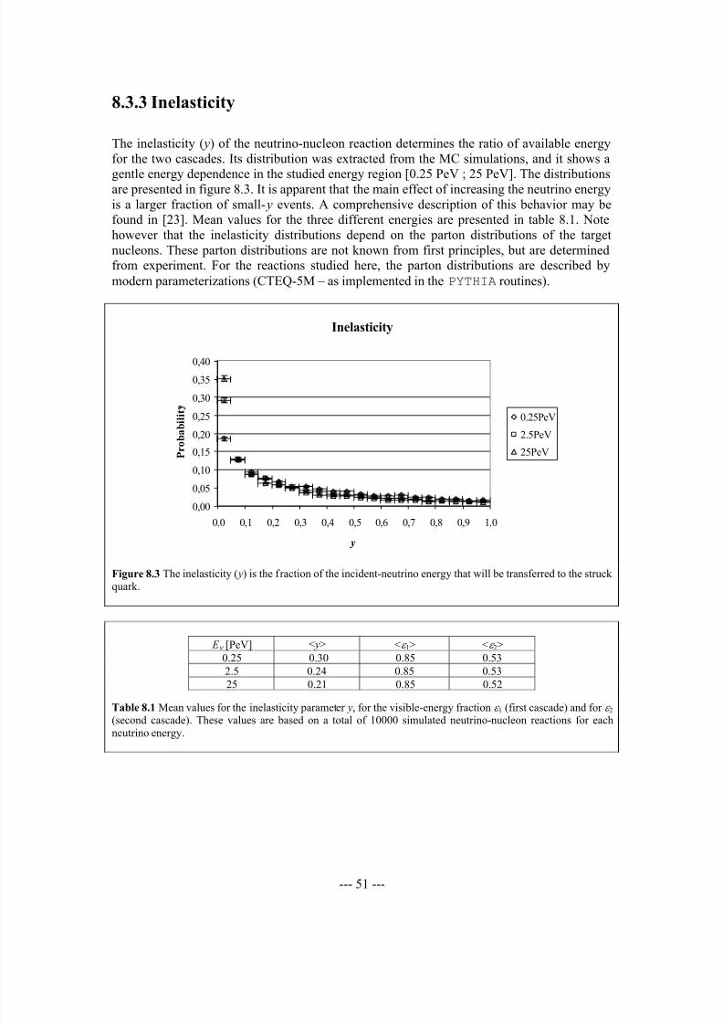
8/3/2019 Pär Lindahl- Energy Calibration of Neutrino Telescopes Using Ultra High Energy Tau Neutrinos
http://slidepdf.com/reader/full/paer-lindahl-energy-calibration-of-neutrino-telescopes-using-ultra-high-energy 56/81
--- 51 ---
8.3.3 Inelasticity
The inelasticity ( y) of the neutrino-nucleon reaction determines the ratio of available energy
for the two cascades. Its distribution was extracted from the MC simulations, and it shows a
gentle energy dependence in the studied energy region [0.25 PeV ; 25 PeV]. The distributionsare presented in figure 8.3. It is apparent that the main effect of increasing the neutrino energy
is a larger fraction of small- y events. A comprehensive description of this behavior may be
found in [23]. Mean values for the three different energies are presented in table 8.1. Note
however that the inelasticity distributions depend on the parton distributions of the target
nucleons. These parton distributions are not known from first principles, but are determined
from experiment. For the reactions studied here, the parton distributions are described by
modern parameterizations (CTEQ-5M – as implemented in the PYTHIA routines).
Inelasticity
0,00
0,05
0,10
0,15
0,20
0,25
0,30
0,35
0,40
0,0 0,1 0,2 0,3 0,4 0,5 0,6 0,7 0,8 0,9 1,0
y
P r o b a b i l i t
0.25PeV
2.5PeV
25PeV
Figure 8.3 The inelasticity ( y) is the fraction of the incident-neutrino energy that will be transferred to the struck
quark.
Table 8.1 Mean values for the inelasticity parameter y, for the visible-energy fraction ε 1 (first cascade) and for ε 2
(second cascade). These values are based on a total of 10000 simulated neutrino-nucleon reactions for eachneutrino energy.
E ν [PeV] < y> <ε 1> <ε 2>
0.25 0.30 0.85 0.53
2.5 0.24 0.85 0.53
25 0.21 0.85 0.52

8/3/2019 Pär Lindahl- Energy Calibration of Neutrino Telescopes Using Ultra High Energy Tau Neutrinos
http://slidepdf.com/reader/full/paer-lindahl-energy-calibration-of-neutrino-telescopes-using-ultra-high-energy 57/81
--- 52 ---
8.3.4 Tauon range
Given the tauon energy and neglecting energy losses along the “tauon track” the expected
tauon range is given by equation (6.2’). For completeness – and as a simple cross-check of the
routines – the tauon mean ranges extracted from the MC simulations were compared with theexpected mean ranges given the extracted mean tauon energies. As expected, the two different
mean-range estimations are found to be consistent with each other (see table 8.2).
Table 8.2 Comparison between mean tauon range and a mean-range estimate based on the mean tauon energy.These values (with statistical errors) are based on a total of 10000 simulated neutrino-nucleon reactions for each
selection of neutrino energy. The two mean-range estimations are found to be consistent with each other.
E ν [PeV] < Rτ > [m] 49m⋅< E τ >/1PeV
0.25 8.481±0.081 8.581±0.043
2.5 92.5±1.5 92.95±0.34
25 968.6±9.7 963.7±5.8

8/3/2019 Pär Lindahl- Energy Calibration of Neutrino Telescopes Using Ultra High Energy Tau Neutrinos
http://slidepdf.com/reader/full/paer-lindahl-energy-calibration-of-neutrino-telescopes-using-ultra-high-energy 58/81
--- 53 ---
Chapter 9
Anticipated event rates
9.1 Motivation
The potential power of the energy calibration method described in chapter 10, depends on the
expected annual number of detected double bang events.
In this chapter I present estimations of the double bang event rates in AMANDA-II and in
IceCube for a typical neutrino spectrum. This is done in three steps:
1) An expression for transforming a neutrino flux to the corresponding double bang
production rate is presented. This expression is then evaluated by performing Monte
Carlo simulations of a large number of neutrino reactions.
2) A simple analytical model is presented describing the effective detector volume for
double bang events. A Monte Carlo program is then used to simulate the detector
responses and estimate the free parameters of this model with respect to AMANDA-IIand IceCube.
3) The anticipated event rates for these two detectors are calculated using the production
rate and effective volume expressions obtained in steps 1 and 2.
9.2 Double bang production rate
9.2.1 Model
The flux of cosmic tau neutrinos is often parameterized asa
νννν
E Φ E Φ
−
⋅=
PeV1)( 1 1112 sr PeVyr m
−−−− ⋅⋅⋅ , (9.1)
[15] where proposed values on the constant 1νΦ may be obtained from section 2.5 for fluxes
with a = 2. (A power-law spectrum with a spectral index ∼2 is typical for sources where
particles have been accelerated in supersonic shocks [16].)

8/3/2019 Pär Lindahl- Energy Calibration of Neutrino Telescopes Using Ultra High Energy Tau Neutrinos
http://slidepdf.com/reader/full/paer-lindahl-energy-calibration-of-neutrino-telescopes-using-ultra-high-energy 59/81
--- 54 ---
The corresponding double bang production rate is
ν
τ
ντ νντ E
E
E E σ E Φ N E n ∫ ⋅⋅⋅⋅= d
d
);(d)()( CC
Adb ρ ε 1113 sr PeVyr m −−−− ⋅⋅⋅ . (9.2)
In this expression an approximate value ρ ≈ 0.92⋅103 kg/m3 (at -4°C, 1 atm) was used for the
density of ice; N A = 6.022⋅1026
kg-1
is the Avogadro constant; ε ≈ 0.83 is the fraction of tauon
decays that result in a cascade
*
; τ ντ E E E σ
d/);(d CC is the differential CC cross section for aneutrino of energy ν E to convert to a tauon of energy τ E .
9.2.2 Simulations
To evaluate equation (9.2), a Monte-Carlo simulation of tau neutrino reactions was performed
using the generator gen_nutau described in section 7.2. The total simulated energy range
was PeV25PeV1.0 << ν E . In this range the reaction cross-section is not constant and this
must, for technical reasons**, be taken into account already in the set-up of the simulation.
As a first step, the energy dependence of the cross-section must therefore be described. In
[22] the CETEQ4-DIS cross-sections are tabulated. I used these values to perform a least-
square fit to the following parameterization:b
νν
E σ E σ
⋅=
PeV1)( 1tot m
2; PeV100PeV1.0 << ν E (9.3)
The model parameters thus obtained are: σ 1 = 8.77⋅10-38
m2
and b = 0.435. For
PeV100PeV25.0 << ν E this expression does not differ from any of the tabulated values
with more than 6%, and at PeV1.0=ν E the difference is 15%. For this parameterization the
total number of neutrino reactions may be expressed as
ν
ab
νν A E E Φ N n d
PeV111tot
−
∫
⋅⋅⋅⋅= σ ρ
113 sr yr m −−− ⋅⋅ . (9.4)
Thus, in the simulation tau neutrino energies are picked from the distribution
α
α α
α −−− ⋅
−= νν E
E E E f
1
1
1
2
-1)( PeV
-1, (9.5)
where E 1 = 0.1 PeV, E 2 = 25 PeV and α = a-b = 1.57.
*The remaining 17% of the tauon decays are given by τ µ ν ν µ τ ++→ .
**Neutrino energies are picked from a distribution, and are forced to interact with a nucleon. To account for the
fact that the probability for interaction is different at different neutrino energies, the shape of the initial neutrino
spectrum must be modified.

8/3/2019 Pär Lindahl- Energy Calibration of Neutrino Telescopes Using Ultra High Energy Tau Neutrinos
http://slidepdf.com/reader/full/paer-lindahl-energy-calibration-of-neutrino-telescopes-using-ultra-high-energy 60/81
--- 55 ---
The number of tau neutrino reactions generated was K = 10000, and the event files
produced by the generator were analyzed using the program ana_db described in section 7.4.
As a result a histogram was produced, representing the tauon-energy distribution for those
events where the tauon did not decay to a muon (and two neutrinos): k ( E τ ) denotes the number
of events in a bin centered at E τ , with the bin widths set to PeV5.0=∆ E . The histogram was
used to evaluate the tauon production rate according to the following expression:
totdb
)()( n
E K
E k E n τ
τ ⋅∆⋅
= 1113 sr PeVyr m −−−− ⋅⋅⋅ , (9.6)
where in this case 11-3
1
7
tot sr yr m1003.3 −−− ⋅⋅⋅⋅= νΦn according to (9.4).
9.2.3 Result
The double-bang production rate for a flux normalized to Φ ν 1 = 1 1112 sr PeVyr m −−−− ⋅⋅⋅ , is
presented in figure 9.1. The bin width is PeV5.0=∆ E . Also included in the plot is a least-
square fit to the parameterization α
τ τ
E n E n
′−
⋅=
PeV1)( 1db 1113 sr PeVyr m −−−− ⋅⋅⋅ . (9.7)
This fit was made for PeV24PeV1 << τ E - i.e. excluding two bins in each end of the
spectrum – a restriction introduced to avoid the cut-off region, due to the limitation in thesimulated neutrino-energy interval. The production rate at 1 PeV and spectral index was
found to be 8
1 1024.4 −⋅=n 1113 sr PeVyr m −−−− ⋅⋅⋅ and 64.1=′α respectively. This
expression will be used in chapter 10 for the analysis of the relation between tauon ranges andtauon energies.
Double Bang Production Rate
1,0E-11
1,0E-10
1,0E-09
1,0E-08
1,0E-07
1,0E-06
0 5 10 15 20 25
E τ
[PeV]
n d b [ m - 3y
r - 1P
e V - 1s
r - 1]
Figure 9.1 The anticipated double-bang production rate assuming a generic Φ ν1⋅( E ν /1 PeV)
-2tau neutrino flux,
with Φ ν 1 = 1 m-2⋅yr
-1⋅PeV-1⋅sr
-1. The dots are the simulated values and the line represents a least-square fit to
ndb( E τ ) = n1⋅( E τ /1 PeV)-1.64
, for 1 PeV < E τ < 24 PeV. The differential event rate at E τ = 1 PeV was found to be
n1 = 4.24⋅10-8
m-3
yr -1
PeV-1
sr -1
.

8/3/2019 Pär Lindahl- Energy Calibration of Neutrino Telescopes Using Ultra High Energy Tau Neutrinos
http://slidepdf.com/reader/full/paer-lindahl-energy-calibration-of-neutrino-telescopes-using-ultra-high-energy 61/81
--- 56 ---
9.3 Effective volume
9.3.1 Model
A double bang event is characterized by the amount of photons produced in the two cascades,and by the cascade separation (tauon range). As was suggested in section 6.2, to be consideredas “detected” an event should be fully contained within the detector volume, the separationshould exceed a minimum value (r min) and both cascades should be energetic enough to bedetected.
To estimate the expected detection rate (ndet), the production rate per unit volume(ngen/V gen) is multiplied with the effective detector volume (V eff ). Given that essentially allcascades are energetic enough for detection – and this is assumed to be the case from hereon – the effective volume will only depend on the tauon energy:
gen
gen
detτeff
)(
)()( V
E n
E n E V
τ
τ ⋅= (9.8)
A phenomenological model for V eff may be obtained by considering a simplifiedsituation: Consider a tau neutrino flux directed perpendicular to a flat detector with anexposed area Aeff and a thickness L. A tauon track of length r will only be fully contained if the tauon is produced no “deeper” than ( L – r ) measured from the surface facing the neutrino
source. This limits the detection volume for such tracks to Aeff ×( L – r ). By weighting thisvolume with the range probability density according to equation (6.3), and integrating over the allowed range interval the final expression is found:
[ ]∫ −−
−
⋅+⋅−−=⋅⋅−=
L
r
R L Rr Rr
τ e Re Rr L Ar R
er L A E V
min
min //
mineff
/
eff eff )(d)()( , (9.9)
where R = R( E τ ) is the mean range according to equation (6.2’).
Since r min is assumed to be a known limitation of the detection process, equation (9.9)suggests that the (energy dependent) effective volume is defined only by the exposed area( Aeff ) and the thickness ( L) of the detector.
9.3.2 Simulations
A series of Monte Carlo simulations were performed using the program veff_mc described
in section 7.3. The purpose for these simulations was to meet two objectives:1) to verify that the equation (9.9) is valid when considering the three-dimensional nature
of the detector and of the tauon production.2) to determine the model parameters Aeff and L for both AMANDA-II and IceCube.
8/3/2019 Pär Lindahl- Energy Calibration of Neutrino Telescopes Using Ultra High Energy Tau Neutrinos
http://slidepdf.com/reader/full/paer-lindahl-energy-calibration-of-neutrino-telescopes-using-ultra-high-energy 62/81
--- 57 ---
In the simulations tauon energies were selected in steps of 0.5 PeV in the interval
0.5 PeV ≤ E τ ≤ 15 PeV. For each energy-selection the simulation continued until 10000 eventshad been detected, detection criteria being: fully contained tauon track, and cascadeseparation exceeding r min. Tauon tracks were generated in a volume (V gen) surrounding thedetector, with directions of origin picked from an isotropic distribution from the upper hemisphere.
For AMANDA-II the following settings were used:
• Detector geometry and dimensions: cylinder; height 500 m, radius 100 m
• Minimum cascade separations: r min = 100 m or 250 m
• Generation volume: V gen = 1.6⋅108
m3
(∼10× the physical detector volume)
For IceCube the following settings were used:
• Detector geometry and dimensions: cylinder; height 950 m, radius 550 m
• Minimum cascade separations: r min = 100 m or 250 m
• Generation volume: V gen = 9.0⋅109
m3
(∼10× the physical detector
volume)
For each simulation the effective volume was calculated according to equation (9.8), withngen equal to the number of generated events necessary to obtain the required number of detected events: ndet = 10000.
9.3.3 Results
For each of the two simulated detectors – with the relevant detector parameters given insection 9.3.2 – the model parameters ( Aeff and L) were obtained by performing a least square
fit of expression (9.9) to the simulation results (see figure 9.2). The results for the twodetectors are:
• AMANDA-II (r min = 100 m): Aeff = 3.87⋅104
m2.
L = 261 m.
• AMANDA-II (r min = 250 m): Aeff = 3.83⋅103 m2. L = 421 m.
• IceCube (r min = 100 m): Aeff = 8.96⋅105
m2.
L = 928 m.
• IceCube (r min = 250 m): Aeff = 8.08⋅105
m2.
L = 962 m.
From the plots in figure 9.2 it is clear that the effective volume for these two detectors iswell described by equation (9.9). Apparently the essential properties of these detectors are preserved in the mathematical model, despite the simplifications made in deriving it. Thegeometry (cylindrical, cubic etc) and size of a detector in combination with the value of theminimum cascade separation r min determines both the “shape” of the energy dependenteffective volume and the normalization factor. For a given r min value the shape may berecreated in the effective-volume function (9.9) by variation of the effective length parameter,
L. The normalization factor may be recreated by variation of the effective area parameter, Aeff .

8/3/2019 Pär Lindahl- Energy Calibration of Neutrino Telescopes Using Ultra High Energy Tau Neutrinos
http://slidepdf.com/reader/full/paer-lindahl-energy-calibration-of-neutrino-telescopes-using-ultra-high-energy 63/81
--- 58 ---
AMANDA-II (r min = 100 m)
0
200 000
400 000
600 000
800 000
1 000 000
1 200 000
1 400 000
0 1 2 3 4 5 6 7 8 9 10 11 12 13 14 15 16
E τ [PeV]
V e f f [ m
3 ]
AMANDA-II (r min = 250 m)
0
10 000
20 000
30 000
40 000
50 000
60 000
70 000
80 000
0 1 2 3 4 5 6 7 8 9 10 11 12 13 14 15 16
E τ [PeV]
V e f f [ m
3 ]
IceCube (r min = 100 m)
0
50 000 000
100 000 000
150 000 000
200 000 000
250 000 000
300 000 000
350 000 000
400 000 000
0 1 2 3 4 5 6 7 8 9 10 11 12 13 14 15 16
E τ [PeV]
V e f f [ m 3 ]
IceCube (r min = 250 m)
0
20 000 000
40 000 000
60 000 000
80 000 000
100 000 000
120 000 000
140 000 000
160 000 000
180 000 000
0 1 2 3 4 5 6 7 8 9 10 11 12 13 14 15 16
E τ [PeV]
V e f f [ m 3 ]
Figure 9.2 Effective detector volumes for double bang events in AMANDA-II and in IceCube. Two different
values for the minimum cascade separation (r min) are considered. Diamonds represent the simulation results.
Lines represent the least square fits of the proposed two-parameter ( Aeff and L) model.
9.4 Event rate calculations
The anticipated double bang event rates ( N db) can now be calculated by multiplying the tauon production rate obtained in section 9.2 with the effective volumes obtained in section 9.3, andintegrating over the relevant tauon energy range. In principle one should also integrate over all solid angles, but this integration was performed numerically when determining the model parameters in the expression for the effective volume. Therefore the solid angle,
Ω ν = 2π steradians for the isotropic neutrino flux from the upper hemisphere, is regarded as aconstant normalization factor in this case:
τ τ τ ν E E V E nΩ N d)()( eff dbdb ⋅⋅⋅= ∫ yr -1
(9.10)
When evaluating the event rate according to (9.10) equation (9.7) was used for the double
bang production rate and equation (9.9) for the effective volume, and the selected energyrange was PeV25PeV25.0 << τ E . Different detector configurations are defined by selecting
the appropriate values for Aeff , r min and L, and different neutrino sources are defined by
selecting the appropriate values for Φ ν 1. The rates are presented in table 9.1 and cover all
combinations of the four neutrino flux estimates introduced in section 2.5 and three different
detector configurations - AMANDA-II, IceCube and a generic detector with the following
characteristics:

8/3/2019 Pär Lindahl- Energy Calibration of Neutrino Telescopes Using Ultra High Energy Tau Neutrinos
http://slidepdf.com/reader/full/paer-lindahl-energy-calibration-of-neutrino-telescopes-using-ultra-high-energy 64/81
--- 59 ---
Aeff = 1 km2
r min = 0.1 km
L = 1 km
The configuration of the generic detector is identical to the one used in [25] for
estimating the detection rate from gamma ray bursts. A direct comparison between estimates
for the maximal GRB flux (Lorentz factor 100= Γ ; labeled “GRB” in table 9.1), shows thatthe stated rate of 0.54 down going double-bang events per year is notably higher than the
value presented here (0.15 yr -1
).
ντ source AMANDA-II
(r min=100m)
AMANDA-II
(r min=250m)
IceCube
(r min=100m)
IceCube
(r min=250m)
“Generic”
(r min=100m)
“Φ ν 1=1” 0.42 yr -1 1.3⋅ 10-2 yr -1 99 yr -1 27 yr -1 123 yr -1
GRB 5.2⋅10-4
yr -1
1.6⋅10-5
yr -1
0.12 yr -1
3.4⋅10-2
yr -1
0.15 yr -1
WB limit 1.0⋅10-3
yr -1
3.3⋅10-5
yr -1
0.25 yr -1
6.7⋅10-2
yr -1
0.31 yr -1
AGN-HC 0.19 yr -1
5.9⋅10-3
yr -1
45 yr -1
12 yr -1
55 yr -1
AM-B10 limit 0.13 yr -1
4.0⋅10-3
yr -1
30 yr -1
8.1 yr -1
37 yr -1
Table 9.1 Typical event rates for different neutrino sources and detector configurations. The “Φ ν 1=1” source
does not correspond to any proposed flux. It is simply a flux normalized to Φ ν 1=1m-2⋅yr
-1⋅PeV-1⋅sr
-1. “GRB” is
the maximum GRB flux according to [25] assuming a mixing scenario where the tau neutrino flux equals half of the generated muon neutrino flux. “WB” is the Waxman-Bahcall upper limit [27] in the same mixing scenario.
“AGN-HC” is the flux from the interior of “optically thick” AGNs (Hidden Core) according to [26] and
assuming maximal mixing. “AM-B10 limit” is the upper limit (extrapolated) obtained by muon-neutrinoobservations with the AMANDA-B10 detector (1997 year data) [28] assuming “distant sources” and maximal
two-flavor mixing (equal amounts of tau neutrinos and muon neutrinos).
9.5 Conclusions
In this chapter a method was presented for deriving the expected double bang event rates
given the neutrino flux and the detector configuration (geometry, dimension and “threshold”).
The rates were also evaluated for a few example fluxes and detector configurations.
One of the results from this evaluation is expression (9.7) for the double-bang energy
distribution. This expression will be used in chapter 10 as part of the information needed to
define a relation between the observed cascade separation and the “expected” visible energy
from the corresponding tauon decay.
From the study of the example detectors a couple of observations can be made about theevent rates. Given the minimum cascade separation r min – essentially defining the energy
threshold – the double bang event rate is not proportional to its volume, but increases faster with volume. The reason is that a larger detector will also be sensitive to events in a wider
energy range. Another possible way of increasing the event rate is to try to resolve events with
smaller values on r min. This both lowers the threshold and increases the detection probability
since short-track events will result from events over the whole energy range.

8/3/2019 Pär Lindahl- Energy Calibration of Neutrino Telescopes Using Ultra High Energy Tau Neutrinos
http://slidepdf.com/reader/full/paer-lindahl-energy-calibration-of-neutrino-telescopes-using-ultra-high-energy 65/81
--- 60 ---
The rates presented in table 9.1 seem to indicate that the double bang event rate will be
too small for calibration purposes in the AMANDA-II detector. One would have to reduce
r min to ∼60 m to reach an event rate of 1 yr -1
at the AMANDA-B10 limit. In IceCube and other
km-scale detectors the event rates will possibly be sufficient if the tau neutrino flux is not
much smaller than what is allowed by the AMANDA-B10 limit. It may be noted that in order
to reach an event rate of 1 yr -1 at the Waxman-Bahcall limit in a generic 1 km3
detector one
would have to reduce r min to ∼25 m.
Finally, using the concept of effective volume, it is possible to make a rough estimate of
the signal-to-background ratio. In section 6.1.1 it was stated that the most serious background
events will be muon neutrino CC events where the muon travels approximately 100 m before
loosing most of its energy in a single bremsstrahlung reaction. According to [7] the fraction of
muon neutrino CC events having a signature similar to this is expected to be of the order 3
fakeCC 103−
→ ⋅= P .
The effective volume for double bang events with a cascade separation of 100 m is
roughly7
100 101⋅=V m3
for AMANDA-II and8
100 108 ⋅=V m3
for IceCube. Assuming equal
amounts of tau neutrinos and muon neutrinos (and similar CC cross-sections) the signal-to-noise ratio may be estimated by the following expression:
100fakeCC
eff )()(
V P
E V E SN
⋅⋅
=→
τ τ
ε , (9.11)
where ε ≈ 0.83 is the fraction of tauon decays that result in a cascade.
For r min = 100 m the energy threshold is roughly E τ ≈ 2 PeV (the tauon energy
corresponding to a tauon range equal to the minimum separation r min). At this threshold
SN ≈ 30 for AMANDA-II and SN ≈ 80 for IceCube. These SN values will improve if the
threshold is lowered.

8/3/2019 Pär Lindahl- Energy Calibration of Neutrino Telescopes Using Ultra High Energy Tau Neutrinos
http://slidepdf.com/reader/full/paer-lindahl-energy-calibration-of-neutrino-telescopes-using-ultra-high-energy 66/81
--- 61 ---
Chapter 10
Energy calibration
10.1 Motivation
One important objective in neutrino telescopy is to determine the neutrino energy. This is
done in two steps: First the energy of the muon or cascade is determined. Then this energy is
used to estimate the neutrino energy.
For muon tracks at low energies a method for energy calibration has been suggested [53]
that uses muons that stop within the detector. The length of the track segment within the
detector is related to the initial energy of the muon. This independent energy estimation can
be compared with the reconstructed energy obtained by the standard algorithm.
In this chapter a similar calibration method for cascades, using double bang events, will
be described. It relies on the fact that the mean range of the tauon is proportional to the tauonenergy. A measurement of the cascade separation will thus provide an independent energy-
estimation for the cascade energy at the decay vertex.
One potential application involving the detection of double bang events is to try to
estimate the mean value of the inelasticity >< y for UHE neutrino nucleon reactions, which
could provide information about the small x behavior of the nucleon structure function [23].
The inelasticity in an event is given by ντ E E y /1−= according to equation (8.3). The tauon
energy τ E could be estimated from the reconstructed energy of the second cascade and the
neutrino energy ν E could be estimated from the reconstructed energies of both cascades. One
important factor for the success of this type of study is of course an accurate energy
reconstruction algorithm.

8/3/2019 Pär Lindahl- Energy Calibration of Neutrino Telescopes Using Ultra High Energy Tau Neutrinos
http://slidepdf.com/reader/full/paer-lindahl-energy-calibration-of-neutrino-telescopes-using-ultra-high-energy 67/81
--- 62 ---
10.2 Method
10.2.1 Energy estimation
In this study the energy spectrum of the tau neutrino flux is assumed to be known, e.g. from
detection and energy reconstruction of muon neutrinos. As an example, the calibration
method will be evaluated for a typical tau neutrino flux, proportional to 2−ν E .
In section 9.2.3 it was shown that the energy spectrum for the corresponding tauons will
be more “flat” due to the increasing neutrino-nucleon cross section at increasing neutrino
energies. Thus, in accordance with the result presented in section 9.2.3 the tauon flux is
assumed to be proportional toα
τ
− E , where the spectral index 6.1≈α .
An expression may now be derived estimating the visible energy at the tauon decayvertex for a given cascade separation (tauon range). The tauon energy estimates are found by
optimizing for smallest possible r.m.s. errors. (Note that other ways to define an estimate are
possible, depending on the purpose of the study.) Given the tauon energy the visible energy at
the tauon decay vertex is then estimated by a constant fraction of the tauon energy:
τ ε E E
vis⋅>=< , (10.1)
where <ε > = 0.53 is the mean value of the probability distribution presented in section 8.3.2.
First the prior probability distribution for the tauon energy is defined as
α
τ α α
α −−− ⋅
−−
= E E E
E f τ 1
1
1
2
1)( ; E 1 < E τ < E 2 , (10.2)
where the energy interval E 1 < E τ < E 2 should cover the sensitive region for the specificdetector. The conditional probability distribution for the tauon range (r ), given the tauon
energy, is presented in equation (6.3):
Rr
τ e R
E r f −
⋅=1
)( ; τ
τ
τ E ct cm
E R
C
τ ⋅=⋅==
4 4 34 4 21
1
GeV)/µm03.49(2
(10.3)
From Bayes’ theorem one can now obtain the conditional probability distribution for E τ, given
the tauon range:
τ α
τ
E C r
τ τ E
E
τ τ
τ τ
τ e E E f E r f
E E f E r f
E f E r f r E f 1
2
1
/)1()()(
d)()(
)()()(
−+− ⋅∝⋅∝
⋅⋅
⋅=
∫ . (10.4)
In general it is now possible to use equation (10.4) to define a suitable energy estimate,
depending on the purpose of the study. For example, since )( r E f τ has a maximum value,
one may want to use this most probable value. Another possibility is to calculate the mean
value. In the present study an energy estimate with a narrow error distribution is favorable.
Thus, the Least-Square (LS) estimate of the tauon energy )~
( τ E is selected, which is
determined by minimizing

8/3/2019 Pär Lindahl- Energy Calibration of Neutrino Telescopes Using Ultra High Energy Tau Neutrinos
http://slidepdf.com/reader/full/paer-lindahl-energy-calibration-of-neutrino-telescopes-using-ultra-high-energy 68/81
--- 63 ---
+⋅⋅⋅=⋅⋅⋅−=
=
∫ ∫ 4 4 4 4 34 4 4 4 21
1
2
1
2
1
d)()(d)()()~
()~
(222
I
E
E
τ τ τ τ τ τ τ τ
E
E
τ τ E E f E r f E E E f E r f E E E χ
4 4 4 4 34 4 4 4 214 4 4 34 4 4 21
3
2
1
2
2
1
d)()(~
2d)()(~2
I
E
E
τ τ τ τ τ
I
E
E
τ τ τ τ E E f E r f E E E E f E r f E
==
∫ ∫ ⋅⋅⋅−⋅⋅ (10.5)
32
2
2~
2~0 I I E E d
d τ
τ
−==χ
⇒
⇒
∫
∫
−+−
−−
⋅
⋅
==2
1
1
2
1
1
d
d
)(~
/)1(
/
2
3 E
E
E C r
E
E
E C r
τ
E e E
E e E
I
I r E
τ
α
τ
τ
α
τ
τ
τ
(10.6)
The integrals on the right side of equation 10.6 were evaluated numerically for different
tauon ranges, m1000m100 ≤≤ r . The selected limits of integration were E 1 = 0.1 PeV and E 2 = 100 PeV, thus covering the sensitive region for the telescopes studied in this thesis. The
results were used to calculate )(~
r E τ for the selected values on r , and a second order
polynomial fit (requiring 0)0(~
=τ E ) was determined:
2)(~
br ar r E +=τ , (10.7)
with the parameter values a = 0.0281 PeV/m and b = -7.33⋅10-6
PeV/m2.
Finally, these tauon energies were converted into visible-energy estimates ( E R) using the
average visible-energy fraction according to equation (10.1)*:
)()(~
)( 2br ar r E r E R +⋅>=<⋅>=< ε ε τ (10.8)
The final result is presented in figure 10.1. In this plot one may note that since the distributionseems to be denser below the line representing the LS estimates, the corresponding meanvalue estimates would probably point at lower energies.
*This approach is a simplification that disregards the prior distribution of the visible energy.

8/3/2019 Pär Lindahl- Energy Calibration of Neutrino Telescopes Using Ultra High Energy Tau Neutrinos
http://slidepdf.com/reader/full/paer-lindahl-energy-calibration-of-neutrino-telescopes-using-ultra-high-energy 69/81
--- 64 ---
Energy Estimation
0
5
10
15
20
25
0 100 200 300 400 500 600 700 800 900 1000 1100
r [m]
E v i s [ P e V ]
Figure 10.1. The visible energy ( E vis) at the tauon decay vertex may be estimated in double-bang events from theseparation between the two cascades (the tauon range, r ). A least-square estimate was determined and
parameterized, assuming a neutrino flux Φ ν ∝ E ν -2
. The result is: E R = <ε >⋅(a⋅r + b⋅r 2), where <ε > = 0.53,
a = 0.0281 PeV/m and b = -7.33⋅10-6
PeV/m2. Also shown is a sample of simulated (r , E vis) points representing
detected double-bang events in IceCube, with r > 100 m.
10.2.2 Simulation
Five simulation runs were made using the Monte Carlo program gen_nutau. In each
simulation 50000 neutrino-nucleon reactions were generated. The double bang information
was extracted using the program ana_db. These double bang events were then processed by
the program dbdet simulating the detection process in IceCube. This program assigns a
position for the first cascade of each event. These positions are selected from a homogenous
distribution inside a cubic generation volume surrounding the detector volume. A direction-
of-origin is selected from an isotropic distribution from the upper hemisphere, and the
position of the second vertex is determined. An event is then labeled “detected” if three
detection criteria are fulfilled:
• Both vertices are found within the detector volume.
• The separation exceeds a minimum separation r min = 100 m.
• Both cascades have visible energies exceeding 1 TeV.
Since the generation volume must be much larger than the detector volume to reduce theedge effects only a fraction of the events will be detected. With a generation volume ten times
as large as the detector the dbdet program was allowed to “reuse” the generated double-
bang events ∼10 times. Each event is then expected to have its first cascade within the
detector volume once (on average).

8/3/2019 Pär Lindahl- Energy Calibration of Neutrino Telescopes Using Ultra High Energy Tau Neutrinos
http://slidepdf.com/reader/full/paer-lindahl-energy-calibration-of-neutrino-telescopes-using-ultra-high-energy 70/81
--- 65 ---
10.2.3 Analysis
After applying the detection procedure 5000 events remained. (1000 events were produced
from each 50000-event simulation.) These double-bang events were analyzed using the
program histo_RE, which produces a histogram for log10( E vis/ E R ). The program offers theoption of introducing “measurement errors”, and this option was invoked to mimic the
expected uncertainties in both r (Gaussian error distribution, σ = 5 m) and log10( E vis/1PeV)
(Gaussian error distribution, σ = 0.2). The error distributions used was taken from [48] which
presents the reconstruction performance for contained cascades in AMANDA-II.
This histogram (using simulation data) would in a in the actual calibration situation be
compared with a corresponding histogram for the reconstructed data. In the ideal situation
these two histograms are expected to be samples from the same distribution. If the method for
reconstructing cascade energies is not ideal this will affect the distribution. In particular, if the
proportionality constant converting a cascade “size” into “energy” is not correct this will have
the effect of shifting the mean value of the distribution.
10.3 Results
10.3.1 Calibration performance
As an example calibration scenario the prospect of identifying a generic defect in the
reconstruction algorithm for E vis will be examined – a misadjusted proportionality constant.
The expected distribution for log10( E vis/ E R) using an ideal reconstruction algorithm (see
figure 10.2) was obtained for double-bang events in IceCube (r min = 100 m) with uncertainties
in both r and E vis included. The mean (m0 = -0.31)*
and r.m.s. value (σ 0 = 0.51) was
determined. These numbers may be used to test the standard reconstruction algorithm. For an
algorithm that does not produce the proper proportionality between reconstructed and true
values of E vis, the distribution will suffer a shift (∆m) of its mean value.
* The mean m0 is negative since the definition of E R results in larger energy estimates than would an alternative
mean value estimate. (A mean value estimate would have the drawback of resulting in a wider distribution.)

8/3/2019 Pär Lindahl- Energy Calibration of Neutrino Telescopes Using Ultra High Energy Tau Neutrinos
http://slidepdf.com/reader/full/paer-lindahl-energy-calibration-of-neutrino-telescopes-using-ultra-high-energy 71/81
--- 66 ---
Calibration Precision
0
50
100
150
200
250
300
350
400
450
500
-6 -5 -4 -3 -2 -1 0 1 2 3 4 5 6
log1 0 ( E vi s / E R )
# E v e n t s
Figure 10.2. Distribution for log10( E vis/ E R) assuming correctly reconstructed double-bang events in IceCube(r min = 100 m). E vis is the measured cascade energy in the second cascade. E R is the second-cascade energy as
estimated from the measured tauon range. The “center-of gravity” is positioned at -0.31, and the r.m.s. value is0.51.
After detecting N db double bang events the mean value is estimated by
m = <log10( E vis/ E R)>, and ∆m is estimated by (m-m0). The minimum shift ∆mmin that may be
detected from this number of events depends on the aspired confidence level (CL). Given the
approximation of regarding log10( E vis/ E R) to be an observation of a Gaussian distribution with
standard deviation σ 0, a significant shift ∆mmin = |m-m0| at 90% CL is
db
0min
96.1
N
σ m
⋅=∆ . (10.9)
This corresponds to a systematic error in the reconstruction of a factor ε ±1
= 10±∆mmin. Given a
tau neutrino flux corresponding to the AMANDA-B10 limit presented in table 9.1 a one-year
(live time) data sample will yield 18.0min
=∆m . In other words, if the standard reconstruction
method under-estimates cascade energies by 30% or over-estimates by 50% this could be
revealed by this method after a one-year exposure.

8/3/2019 Pär Lindahl- Energy Calibration of Neutrino Telescopes Using Ultra High Energy Tau Neutrinos
http://slidepdf.com/reader/full/paer-lindahl-energy-calibration-of-neutrino-telescopes-using-ultra-high-energy 72/81
--- 67 ---
Chapter 11
Summary and outlook
The main topic for this thesis has been to try to investigate the prospects for energy
calibration of cascade events in large neutrino telescopes, using cosmic tau neutrinos. In order
to do so, three questions were formulated.
1) Are tau neutrinos of sufficient energy ( ∼ 1 PeV) produced in nature?
Probably there does not exist any major production sites for “prompt” tau neutrinos.
However, due to a phenomenon called neutrino mixing, which predicts that neutrinos will
“oscillate” between neutrino “flavors” during propagation through space, it is not unlikely that
all three flavors are equally abundant, as long as one only considers sources outside our solar
system.
The expected flux contributions from such sources may be estimated in different ways.
For individual source candidates theoretical models may be used to try to estimate their flux
contributions. Examples on phenomena that has been modeled in this way are Gamma Ray Bursters (GRB) and Active Galactic Nuclei (AGN). For classes of source candidates one may
e.g. use the observed flux of the high-energy Cosmic Rays (CR) to put limits on the neutrino
flux. This approach has e.g. been used to derive an upper bound, which constrains the total
neutrino flux from optically “thin” sources (first done by E. Waxman and J. Bahcall). The
most straightforward approach, finally, is to try to constrain the neutrino flux through direct
neutrino observations. One example is the upper limit derived from AMANDA-B10 (an
earlier stage of AMANDA) data, taken during the austral winter 1997.
2) Will present or future neutrino telescopes be able to detect these tau neutrinos?
To answer that question one has to investigate the properties of such neutrino telescopes.
In this thesis two detectors are described – AMANDA which has been deployed in the glacier ice near the geographical South Pole and IceCube which is a planned extension to AMANDA
and will be deployed at the same location. These detectors use a detection technique of
registering the emission of Čerenkov photons. This radiation is produced as electrically
charged particles propagate through matter, e.g. as the electrically charged daughters from a
neutrino-nucleon reaction propagate through the detector medium (ice).

8/3/2019 Pär Lindahl- Energy Calibration of Neutrino Telescopes Using Ultra High Energy Tau Neutrinos
http://slidepdf.com/reader/full/paer-lindahl-energy-calibration-of-neutrino-telescopes-using-ultra-high-energy 73/81
--- 68 ---
The “signature” of these events depends on the flavor of the parent neutrino. Electron
neutrinos result in single “cascade” events where the energy is deposited locally in the
vicinity of the initial interaction vertex. Muon neutrinos will (in the case of charged current
reactions) result in “track” events since the muons produced from these reactions are heavier
then electrons and therefore more “penetrating”. Tauons are heavier still, and one would
expect tau neutrino reactions to produce tracks events as well. However, since the lifetime of
a tauon is very small it will decay (producing a second cascade) before reaching very far, andthus retaining most of its initial energy. At relativistic energies time dilation becomes
important, and the tauon range is proportional to its energy. The resulting signature will be
two cascades separated by a tauon track. This is referred to as the “double-bang” signature.
Double bang events are at focus in this thesis, due to the useful linearity between the
tauon energy and its range. By measuring the cascade separation it is possible to predict the
energy of the second cascade (at the tauon decay vertex). This energy estimate may then be
compared with the measured energy of the same cascade. Eventually – when enough statistics
has been gathered – it is in principle possible to calibrate the method used for measuring
cascade energies.
The principle is clear, and the next step is to try to estimate the annual number of double bang events. To do so one needs to know two things – the event rate in the detector medium
and the detection probability. Both of these are energy dependent.
The event rate is expected to be described by a power law formula α -
db d/d τ τ E E N ∝
where the spectral index 6.1≈α . Typical neutrino flux estimates were taken from the
literature, but in the present study Monte Carlo simulations were used convert the given
neutrino flux estimates to their corresponding double bang event rates.
The detection probability is expressed as an effective volume V eff . It is defined as the
volume, which multiplied with the double bang event rate per unit volume, yields the double
bang detection rate (both cascades contained within the physical detector volume). Anapproximate expression for the effective volume was derived in this thesis. It has three free
parameters. One of these – the minimum detectable cascade separation r min – is assumed to be
a known property of the detector. The other two – the detector “thickness” L and the
“effective area” Aeff – was determined through Monte Carlo simulations. For AMANDA-II
(the present – year 2003 – configuration of AMANDA) with m100min=r (an ad hoc value)
the thickness and effective area were found to be L ≈ 260 m and Aeff ≈ 3.9⋅104
m2
respectively.
The effective volume rises sharply with increasing tauon energies, peaks at PeV3≈τ E
(V eff ≈ 1.2⋅106 m3 – about 8% of the physical volume) and then falls off slowly with energy.
For the proposed IceCube detector with a geometric volume approaching 1 km3, m100min =r
resulted in L ≈ 930 m and Aeff ≈ 9.0⋅105
m2. IceCube was found both to be “sensitive” in a
wider energy range compared with AMANDA-II. The peak value of the effective volume is positioned at PeV5.5≈τ E (V eff ≈ 3.5⋅10
8m
3– about 39% of the physical volume).
8/3/2019 Pär Lindahl- Energy Calibration of Neutrino Telescopes Using Ultra High Energy Tau Neutrinos
http://slidepdf.com/reader/full/paer-lindahl-energy-calibration-of-neutrino-telescopes-using-ultra-high-energy 74/81
--- 69 ---
Finally, by assuming an isotropic neutrino flux from “above” – the earth is essentially
opaque to neutrinos at these energies and thus shields off the upward going neutrinos –
enough information is at hand to estimate the detection rates for different proposed neutrino
sources and neutrino flux upper limits. To exemplify, for AMANDA-II (with m100min =r )
the AMANDA-B10 upper limit corresponds to 0.13 detected double bang events per year.
IceCube (with m100min =r ) this flux corresponds to 30 double bang events per year.
3) Can the double bang signature be used for calibration purposes?
In this thesis it is assumed that double bang events may be detected and recognized as
such, and that the essential information may be “extracted” from data. The prospects for the
proposed calibration method then relies on an essentially background free signal, a
sufficiently high detection rate and a reasonably narrow distribution in the energy prediction
based on the cascade separation.
The most serious background is assumed to come from charged current muon neutrino
reactions where the muon travels approximately 100 m before loosing most of its energy in a
single bremsstrahlung reaction. Rough calculations of the signal to noise ratio at the energythreshold for the detectors, ∼ 2 PeV, yield a value of ∼ 30 for AMANDA-II (with
m100min =r ) and ∼ 80 for IceCube (with m100min =r ). These values will improve if the
minimum separation r min is smaller than the assumed value.
The detection rates will clearly be too low for calibration purposes in the AMANDA-II
detector. However, one must not forget that there is still at least one free parameter that might
change this situation. To reach a possible detection rate of one double bang event per year (at
the AMANDA-B10 upper limit) r min would have to be close to ∼ 60 m. For IceCube size
detectors it is meaningful to investigate what it would take to be able to detect more
pessimistic (realistic) flux estimates. E.g., to reach a detection rate of one double bang event
per year at the Waxman-Bahcall limit in a 1 km3
detector r min would have to be close to
∼ 25 m. This separation is similar to the expected (longitudinal) cascade lengths and istherefore probably very difficult to reach.
One may also argue that the detection rates will be larger if it turns out that the restriction
of assuming fully contained events are too strict. It has been demonstrated that single cascades
can be reconstructed even if they occur slightly outside the physical volume of the detector.
However, since the uncertainties are larger in the reconstruction of position and energy of
such cascade events, non-contained double bang events will probably not be suitable for
calibration purposes.

8/3/2019 Pär Lindahl- Energy Calibration of Neutrino Telescopes Using Ultra High Energy Tau Neutrinos
http://slidepdf.com/reader/full/paer-lindahl-energy-calibration-of-neutrino-telescopes-using-ultra-high-energy 75/81
--- 70 ---
The detection rates necessary for the proposed application – energy calibration of high
energy cascades – depends on the possibility to determine the position and energy of the two
cascades. It also depends on the intrinsic properties of the double bang events – how well the
energy of the second cascade (at the tauon decay vertex) can be estimated from the cascade
separation. For the precision and accuracy of determining the cascade positions, and for the
precision in of the measurement of the cascade energy, values were assumed to be similar to
what has been demonstrated for single cascades. This is clearly an optimistic assumption, butthe important thing is not the quality of the measurement in it self so much as knowing what
the quality is. The applicability of the calibration method will most likely be limited by the
intrinsic properties. These properties have been determined through Monte Carlo simulations
of neutrino-nucleon reactions.
To be able to examine the calibration method in quantitative terms an expression was
derived for the “optimal” energy estimation as a function of cascade separation. A Monte
Carlo simulation of double bang events, taking into account the described properties of the
detection process, were used to produce “data” for the calibration. For each event the
logarithm of the ratio between the “measured” energy ( E vis) of the second cascade and the
estimated energy ( E R) was calculated. The distribution of these log10( E vis/ E R) values was
found to be (roughly) Gaussian in shape. By observing that if the measured energy is over- or under estimated by a constant factor, this will result in a shift of the mean of this distribution.
The standard deviation thus limits the resolution of the method. For IceCube (with
m100min =r ) a one year exposure to a flux equal to the AMANDA-B10 upper limit a
systematic under-estimation of the measured cascade energies by 30% (or more) will be
detected at 90% CL. Similarly, if the measurement systematically over-estimates cascade
energies by 50% or more, this will also be detected at 90% CL. This example concludes the
study.
To go further it is necessary to evaluate the work already done. The principle of a
calibration method has been demonstrated. Along the way, some phenomenological models
have been developed to assist in studying the expected behavior of neutrino telescopesdetecting double bang events. Also the intrinsic behavior of these events has been described in
a “compact” manner. The next steps should include detailed detector simulations to produce
as realistic “data” as possible. With these at hand one may start experimenting with different
types of filter schemes and reconstruction methods. Then the possibilities for this method to
become a practical method can be put to test. One crucial point is if there is a way to separate
cascades appearing very closely in space. Perhaps the time information (photon hit times on
the optical sensors) could be used in a very elaborate way.
One sub goal should be to try to identify these events accurately enough to be able to
derive upper limits on the tau neutrino flux, thus contributing to the study of neutrino
oscillation. If and when it is possible to detect double bang events at a sufficient rate and
accurately measure their cascade energies and separation it is possible to invoke the proposedmethod for energy calibration.

8/3/2019 Pär Lindahl- Energy Calibration of Neutrino Telescopes Using Ultra High Energy Tau Neutrinos
http://slidepdf.com/reader/full/paer-lindahl-energy-calibration-of-neutrino-telescopes-using-ultra-high-energy 76/81
--- 71 ---
Acknowledgements
In my work with AMANDA in general and in the preparation of this thesis I have received a
lot of support and encouragement from many people around me. First of all I would like to
thank Per-Olof Hulth at Stockholm University for his guidance and for sharing his deep
insight into the experimental side of neutrino astrophysics. My first contact with the
AMANDA-group however, was with Staffan Carius and Allan Hallgren. These inspiring
teachers introduced me to the exciting world of scientific research as they guided me through
my MSc project at Uppsala University. Staffan later became my mentor at Kalmar University,
and he has continued to support and encourage me in my research even though I am no longer
with the university. Even with his help finalizing this thesis would have been much more
difficult without the support – e.g. by granting me very flexible working hours - from my
bosses, Anders Werkström and Anders Rapp, during my two years at OKG AB.
The third “AMANDroid” to join up in Kalmar was Arvid Pohl. In him I have found a
fantastic discussion partner and good friend, a true catalyst for extracting good ideas. Among
the competent and dedicated staff in Kalmar I especially want to thank two of the computer
“gurus”, Claes Johansson and Stefan Petersson, who initially helped in getting the AMANDA
work going by setting up the computer equipment and installing the necessary software. Also,
Bo Rydberg must be acknowledged for his abilities in mechanical issues - constructing
freezing containers and such - which is nothing less than outstanding. Thank you for your
kind help.
I have made two trips to the AMANDA facility in Antarctica. At the Amundsen Scott South Pole Station I have met only capable and friendly people. In particular I have had the
privilege to work closely with my good friend Julio Rodríguez Martino and with Ignacio
Taboada. They shared my efforts regarding the diagnostic measurements on the AMANDA
electronics. Julio and I worked together in November and December 1998, and Ignacio helped
me when I returned one year later.
Regarding my work with simulations of particle reactions and detector responses I am
grateful to Gunnar Ingelman and to Joakim Edsjö who introduced me to the PYTHIA code,
and to Carlos Pérez de los Heros who showed me the ins and outs of amasim. I also want to
thank Ariel Goobar and Lars Bergström for helping me getting a grasp of the big picture, e.g.
by introducing me to some of the potential neutrino sources lurking “out there”. Christian
Walck has been a constant inspiration, especially in the field of mathematical statistics in
which he is conversant both as a pragmatist and as a theoretician. Christian has also, together with Staffan Carius, Per-Olof Hulth and Klas Hultqvist, been my coach in finalizing this
thesis.
Finally, I extend my warm thanks to my mother and father, Ann and Stig Lindahl, for
allowing me to use their den whenever I needed to withdraw from every-day life to do my
scientific scribbling, and to my wife and son, Pia and David Lindahl, for always welcoming
me back!

8/3/2019 Pär Lindahl- Energy Calibration of Neutrino Telescopes Using Ultra High Energy Tau Neutrinos
http://slidepdf.com/reader/full/paer-lindahl-energy-calibration-of-neutrino-telescopes-using-ultra-high-energy 77/81
--- 72 ---
Bibliography
[1] V.A. Balkanov et al., Astroparticle Physics 12 (1999) 75, astro-ph/9903341,
“ Registration of Atmospheric Neutrinos with the BAIKAL Neutrino Telescope NT-96 ”[2] E. Aslanides et al., the ANTARES Collaboration. ANTARES Proposal, “ A Deep Sea
Telescope for High Energy Neutrinos”, astro-ph/9907432
[3] E.G. Anassontzis et al., Nucl. Phys. B (Proc. Suppl.) 66 (1998) 247
[4] T. Montaruli for the NEMO Collaboration, M. Ambriola et al., 26th
ICRC, HE 6.3.06,
“Capabilities of an Underwater Detector as a Neutrino Telescope and for the
Neutrino Oscillation Search”, hep-ex/9905019[5] E. Andres et al., the AMANDA Collaboration, Astroparticle Physics 13 (2000) 1,
“The AMANDA Neutrino Telescope: Principle of Operation and First Results”,
astro-ph/9906203
[6] The IceCube Collaboration, “ IceCube: a Kilometer-Scale Neutrino Observatory, A Proposal to the National Science Foundation”, November 1999
[7] J.G. Learned, S. Pakvasa, Astroparticle Physics 3 (1995) 267, “ Detecting ν τ Oscillations at PeV Energies”, hep-ph/9405296
[8] D. N. Spergel et al., Astrophysical Journal Supplement 148 (2003) 175, “ First Year
Wilkinson Microwave Anisotropy Probe (WMAP) Observations: Determination of Cosmological Parameters”, astro-ph/0302209
[9] S. Perlmutter et al, Astrophys. J. 517 (1999) 565-586, “Measurements of Omega and Lambda from 42 High-Redshift Supernovae”, astro-ph/9812133
[10] M. Tegmark, M. Zaldarriaga, A. J. S. Hamilton, Nuclear Physics B (Proc. Suppl.) 91
(2001) 387-392, “Weighing Neutrinos with Microwave Background and Galaxy Data”
[11] The AMANDA Collaboration, Phys. Rev. D 66 (2002) 032006, “ Limits to the muon flux from WIMP annihilation in the center of the Earth with the AMANDA detector ”,
astro-ph/0202370
[12] L. Bergström, A. Goobar, Cosmology and Particle Astrophysics, Wiley, 1999
[13] A. Letessier-Selvon, Nuclear Physics B (Proc. Suppl.) 91 (2001) 473-479, “ Neutrinosand the Highest Energy Cosmic Rays”
[14] H. Athar, Astropart. Phys. 14 (2000) 217-225, ” Neutrino Conversions in Cosmo-logical Gamma-Ray Burst Fireballs”, hep-ph/0004191
[15] J. G. Learned, K. Mannheim, Annu. Rev. Nucl. Part. Sci. 50 (2000) 679-749, “ High- Energy Neutrino Astrophysics”
[16] Y. A. Gallant, to appear in " Relativistic Flows in Astrophysics", eds. A.W. Guthmann
et al, Lecture Notes in Physics, Springer Verlag, astro-ph/0201243
[17] R. Gandhi, Nuclear Physics B (Proc. Suppl.) 91 (2001) 453-461, “Ultra-High Energy Neutrinos: A Review of Theoretical and Phenomenological Issues”, hep-ph/0011176
[18] K. Hagiwara et al ., Physical Review D 66 (2002) 010001, “The Review of Particle
Physics”, http://pdg.lbl.gov

8/3/2019 Pär Lindahl- Energy Calibration of Neutrino Telescopes Using Ultra High Energy Tau Neutrinos
http://slidepdf.com/reader/full/paer-lindahl-energy-calibration-of-neutrino-telescopes-using-ultra-high-energy 78/81
--- 73 ---
[19] The Super-Kamiokande Collaboration, (Talk presented at 8th
International Workshop
on Neutrino Telescopes, Venice, Italy, 23-26 Feb 1999) Venice 1999, Neutrinotelescopes, vol. 1 183-201, “ Atmospheric Neutrinos at Super - Kamiokande”,
hep-ex/9905016
[20] The SNO Collaboration, Submitted to Physical Review Letters, “Measurement of theTotal Active 8B Solar Neutrino Flux at the Sudbury Neutrino Observatory with
Enhanced Neutral Current Sensitivity”, nucl-ex/0309004[21] The KamLAND Collaboration, Physical Review Letters 90 (2003) 021802, “ First
Results from KamLAND: Evidence for Reactor Antineutrino Disappearance”
[22] R. Gandgi, C. Quigg, M. H. Reno, I. Sarcevic, Phys. Rev. D 58 (1998) 09009,
“ Neutrino Interactions at Ultrahigh Energies”, hep-ph/9807264
[23] J. A. Castro Pena, G. Parente, E. Zas, Physics Letters B 500 (2001) 125-132,
“Measuring the BFKL Pomeron in Neutrino Telescopes”, hep-ph/0011043
[24] J. F. Beacom, P. Crotty, E. W. Kolb, Physical Review D 66 (2002) 021302, “ Enhanced signal of astrophysical tau neutrinos propagating through Earth”, astro-ph/0111482
[25] J. Alvarez-Muñiz, F. Halzen, D. W. Hooper, Physical Review D 62 (2000) 093015,
” High Energy Neutrinos from Gamma Ray Bursts: Event Rates in NeutrinoTelescopes”, astro-ph/0006027
[26] F. W. Stecker, M. H. Salamon, Space Sci. Rev. 75 (1996) 341-355, “ High Energy Neutrinos from Quasars”, astro-ph/9501064
[27] E. Waxman, J. Bahcall, Physical Review D 59 (1999) 023002, ” High Energy Neutrinos from Astrophysical Sources: An Upper Bound ”, hep-ph/9807282
[28] J. Ahrens et al., the AMANDA Collaboration, Physical Review Letters 90 (2003)
251101, “ Limits on Diffuse Fluxes of High Energy Extraterrestrial Neutrinos with the AMANDA-B10 Detector ”, astro-ph/0303218
[29] J. D. Jackson, “Classical Electrodynamics” 2nd
edition, Wiley (1975)
[30] A. Bouchta, PhD Thesis, Stockholm University, Department of Physics (1998),
“Muon Analysis with the AMANDA-B Four-String Detector ”[31] C. Spiering, Nuclear Physics B (Proc. Suppl.) 91 (2001) 445-452, “ Future High
Energy Neutrino Telescopes”, astro-ph/0012532
[32] E. Dalberg, PhD thesis, Stockholm University, Department of Physics (1999), “ ASearch for Neutralino Dark Matter with the AMANDA-B10 Detector ”
[33] K. Woschnagg for the AMANDA collaboration, 26th
ICRC, HE 4.1.15 (1999),
“Optical Properties of South Pole Ice from 140 to 2300 Meters”
[34] P. Niessen, AMANDA – Internal Report 19981101 (1998), “Simulated Bubbles and Their Effect on some Observables in AMANDA-B4”
[35] J. Almlöf, F. Burmeister, Project Report, Uppsala University, Department of Radiation
Sciences (1998), “Minimisation of Air Bubbles in Ice”
[36] P. Lindahl, AMANDA – Internal Report 20031103 (1998), “ Description of bubble formation during freezing of water in a cylindrical container ”
[37] P. Lindahl, MSc Thesis, Uppsala University, Department of Radiation Sciences
(1997), “ Investigation of Timing Properties and Possibilities for Analog Pulse Detection for a Detector Channel of the Neutrino Telescope AMANDA”
[38] P. Lindahl, AMANDA – Internal Report 19980501 (1998), “ Background trigger ratesin AMANDA due to PMT dark noise”
[39] S. Hundertmark, Proceedings of the Workshop on Simulation and Analysis Methods
for Large Neutrino Telescopes DESY-Zeuthen, Germany, July 6-9, 1999, ed.
C. Spiering, DESY-PROC-1999-01, ISSN 1435-8077, “ AMASIM neutrino detector simulation program”

8/3/2019 Pär Lindahl- Energy Calibration of Neutrino Telescopes Using Ultra High Energy Tau Neutrinos
http://slidepdf.com/reader/full/paer-lindahl-energy-calibration-of-neutrino-telescopes-using-ultra-high-energy 79/81
--- 74 ---
[40] P. Lindahl, AMANDA internal note presented in the collaboration meeting June 20-23
1999 in Uppsala, “ ELECTRA, an electronics simulation”
[41] P. Lindahl, AMANDA — Internal Report 20031104 (2000), “ DiagnosticMeasurements and Observations Regarding the Detector Channels in AMANDA B13”
[42] A. Karle, P. Romenesko, AMANDA — Internal Report 19991001, ” Investigation into
the observed gain instabilities of PMTs in the Ice using 1998 data”[43] A.R. Smith, R.J. McDonald, AMANDA — Internal Report 19990201, ” Radioactivities
in AMANDA Optical Module #13-457 ”[44] C. Wiebusch, PhD thesis, Rheinishe Westfälishe Techniche Hochschule AAchen
(1995), “The Detection of Faint Light in Deep Underwater Neutrino Telescopes”
[45] U. Amaldi, Physica Scripta 23 (1981) 409, “ Fluctuations in CalorimetryMeasurements”
[46] "GEANT Detector Description and Simulation Tool ", CERN Program Library:http://cernlib.web.cern.ch/cernlib/
[47] I. Taboada, M. Kowalski for the AMANDA Collaboration, Proceedings of 27th ICRC
(2001), HE 2.3 18:36, “Search for Cascade-like events in the AMANDA-B10 detector ”[48] M. Kowalski, I. Taboada, AMANDA — Internal Report 20020301, ”Cascade
Reconstruction in AMANDA”[49] H. Lai et al. (CTEQ Collaboration), Phys. Rev. D55 (1997) 1280
[50] D. Fargion, Preprint INFN 1166/97 , astro-ph/9704205, “The role of ντ ultrahighenergy astrophysics in km3 detectors”
[51] T. Sjöstrand, Computer Physics Commun. 82 (1994) 74
[52] J. Klug, Diploma thesis, Uppsala University, Department of Radiation Sciences
(1997), “ Enhancement of Up/Down Signal Ratio and Crosstalk Studies in AMANDA”
[53] V. A. Kudryavtsev et al., ” Energy calibration of large underwater detectors using stopping muons”, hep-ex/0010056

8/3/2019 Pär Lindahl- Energy Calibration of Neutrino Telescopes Using Ultra High Energy Tau Neutrinos
http://slidepdf.com/reader/full/paer-lindahl-energy-calibration-of-neutrino-telescopes-using-ultra-high-energy 80/81
--- 75 ---
List of Publications for Pär Lindahl
1997
1. Author: Pär Lindahl
Title: Investigation of Timing Properties and Possibilities for Analog Pulse Detection for a Detector Channel of the Neutrino Telescope AMANDA
Ref.:MSc thesis, Internal report ISV-10/1997, Uppsala University, December 1997
1998
2. Author: Pär Lindahl
Title: Background trigger rates in AMANDA due to PMT dark noise
Ref .: AMANDA – Internal Report 19980501 (1998)
3. Author: Pär Lindahl
Title: Description of bubble formation during freezing of water in a cylindrical
container Ref .: AMANDA – Internal Report 20031103 (1998)
2000
4. Authors: AMANDA Collaboration: E. Andrés et al
Title: The AMANDA Neutrino Telescope: Principle of Operation and First Results Ref.: Astroparticle Physics 13 (2000) 1-20, March 2000
5. Author: Pär Lindahl
Title: Diagnostic Measurements and Observations Regarding the Detector Channelsin AMANDA B13
Ref .: AMANDA — Internal Report 20031104 (2000)

8/3/2019 Pär Lindahl- Energy Calibration of Neutrino Telescopes Using Ultra High Energy Tau Neutrinos
http://slidepdf.com/reader/full/paer-lindahl-energy-calibration-of-neutrino-telescopes-using-ultra-high-energy 81/81
2001
6. Authors: AMANDA Collaboration: E. Andrés et al
Title: Observation of High-Energy Neutrinos Using Cerenkov Detectors Embedded Deep in Antarctic Ice
Ref.: Nature 410 (2001) 441-443, 22 March 2001
2002
7. Authors: AMANDA Collaboration: J. Ahrens et al
Title: Search for Supernova Neutrino-Bursts with the Amanda Detector Ref.: Astroparticle Physics 16 (2002) 345-359, February 2002
8. Authors: AMANDA Collaboration: J. Ahrens et al
Title: Observation of High Energy Atmospheric Neutrinos with the Antarctic Muonand Neutrino Detector Array
Ref.: Physical Review D66 (2002) 012005, 1 July 2002
9. Authors: AMANDA Collaboration: J. Ahrens et al
Title: Limits to the Muon Flux from WIMP Annihilation in the Center of the Earthwith the AMANDA Detector Ref.: Physical Review D66 (2002) 032006, 1 August 2002
2003
10. Authors: AMANDA Collaboration: J. Ahrens et al
Title: Search for Neutrino-Induced Cascades with the AMANDA Detector Ref.: Physical Review D67 (2003) 012003, 1 January 2003
11. Authors: AMANDA Collaboration: J. Ahrens et al
Title: Search for Point Sources of High-Energy with AMANDA
Ref.: Astrophysical Journal 583 (2003) 1040-1057, 23 January 2003
12. Authors: AMANDA Collaboration: J. Ahrens et al
Title: Limits on Diffuse Fluxes of High Energy Extraterrestrial Neutrinos with theAMANDA B10 D t t