palestine polytechnic university college of engineering

Palestine Polytechnic University

College Of Engineering and Technology

Electrical Power Engineering Department

Project Title

Modeling of Smart Grid Lab Using MATLAB/Simulink

Project Team

Muhamad I. Shakarna Bilal N. Abu Awwad

Muhamad M. Jawabra

Project Supervisor

Dr. Maher Al - Maghalseh

Hebron – Palestine

December – 2016

Certificate

Palestine Polytechnic University

The Project Entitled:

Modeling of Smart Grid Lab Using MATLAB/Simulink

By

Muhamad I. Shakarna Bilal N. Abu Awwad

Muhamad M. Jawabra

In accordance with the recommendations of the project supervisor, and the

acceptance of the examining committee members, this project has been

submitted to the Department of Electrical Power Engineering in the college of

Engineering and Technology in partial fulfillment of the requirements of the

department for the degree of Bachelor of Science in Engineering.

Project Supervisor Department Chairman

December-2016

الإهداء

بسم الله الرحمن الرحيم

معلم البشرية ومنبع العلم نبينا محمد )صلّ الله عليه وسلم(

إلـــــى.....

..... آبائنا الأعزاءينابيع العطاء الذين زرعوا في نفوسنا الطموح والمثابر


ب ....... أمهاتنا الأحبةأنهار المحبة التي لا تنض


من يحملون في نفوسهم ذكريات الطفولة والشباب ..... أخوتنا وأخواتنا


كافة الأهل الأصدقاء


تذتنا الأفاضلمن مهّدوا لنا طريق العلم والمعرفة ...... أسا


من ضحّوا بحريتهم من أجل حريتنا ..... أسرانا البواسل


من وصلت رائحة دمائهم الزكية إلى السماء الندية ....شهداؤنا الأبرار

، فإن لم تستطع فأحب العلماء ،فإن فإن لم تستطع فكن متعلما ، "كن عالما

"لم تستطع فلا تبغضهم

:خص بالتقدير والشكرون

د.مـــــــــاهر المغــــــــالسةالدكتور

:الله عليه وسلم نقول له بشراك قول رسول الله صلّ الذي

إن الحوت في البحر ، والطير في السماء ، ليصلون على معلم الناس "

"الخير

، فأنت أهل معناه ، وللإبداع أناس يحصدونه للنجاحات أناس يقدرون

للشكر والتقدير .. فوجب علينا تقديرك .. فلك منا كل الثناء والتقدير

فريق العمل

Abstract

This project concerns the simulation of Renewable Energy Lab at Palestine Polytechnic

University. A simulation is done by deriving the equations of each module used in the lab,

and simulated as blocks using MATLAB/Simulink. The modules considered are (Power

circuit breaker, Maximum power demand, Transmission lines, Loads, Three phase induction

generator, PV module, and Inverter module).

Complete design of Renewable Energy Lab was carried out. The design consist of the

electrical modules that mentioned earlier, and the modules simulated stand alone to achieve

the final form.

Finally several experiments on MATLAB and also practical are done, and a comparison

between the results is obtained. After obtaining the comparison, a results validation is done.

i

Table of Contents

Chapter page

CHAPTER ONE: Introduction 1

1.1 Overview 2

1.2 Motivations 2

1.3 Objectives 2

1.4 Challenges 3

1.5 Importance 3

1.6 Time schedule 4

1.7 Expected results 5

CHAPTER TWO: Smart Grid Lab

6

2.1 Smart Grid Lab Modules

7

2.1.1 Introduction 7

2.1.2 Power circuit breaker

8

2.1.3 Maximum demand meter

8

2.1.4 Line models

9

2.1.5 Three phase transformer & supply unit

10

2.2 Power Electronics and Machinery modules

12

2.2.1 Dc/ac converter (Inverter)

12

2.2.2 Three phase induction machine

13

2.2.3 Loads (R,L,C)

13

2.3 Renewable energy modules

15

ii

2.3.1 PV simulator module 15

2.4 Summary 16

CHAPTER THREE: Modules Simulation 1

17

3.1 Smart grid modules modeling

18

3.1.1 Circuit breaker

18

3.1.2 Power Measurements

21

3.2 Power analysis and theory

39

3.2.1 Harmonics

39

3.2.2 Linear and non-Linear loads

41

3.2.3 Power factor

43

3.3 Summary

45

CHAPTER FOUR: Modules Simulation 2 46

4.1 Loads and Transmission modules

47

4.1.1 Load modules

47

4.1.2 Transmission line modules

53

4.2 Power electronics modules

56

4.2.1 Dc-to-AC converter(inverter) 56

4.2.2 Buck-Boost converter 57

4.2.3 Maximum power point tracker

58

4.2.4 Filter

60

4.3 Renewable energy modules 61

4.3.1 PV panel module 61

4.3.2 Three phase induction machine 62

iii

4.4 Final Form

64

CHAPTER FIVE: Experiments 65

5.1 Loads

66

5.1.1 Introduction

66

5.1.2 R-Load

66

5.1.3 C-Load 68

5.1.4 L-Load

69

5.2 Transmission

71

5.2.1 Short

71

5.2.2 Medium

74

5.2.3 Long

76

5.3 Results Validation

79

5.3.1 Load results

79

5.3.2 Transmission results

84

5.3.3 Validation check 91

5.4 Combined Loads

96

5.5 Conclusion 99

iv

List of Figures

Figure Page

Figure 2.1: Power circuit breaker. 8

Figure 2.2: Maximum demand meter. 8

Figure 2.3: Transmission line model. 9

Figure 2.4: Distribution line model. 10

Figure 2.5: Three phase transformer. 10

Figure 2.6: Three phase supply unit. 11

Figure 2.7: Inverter grid. 12

Figure 2.8: Three phase induction machine. 13

Figure 2.9: Resistive load. 13

Figure 2.10: Inductive load. 14

Figure 2.11: Capacitive load. 14

Figure 2.12: Photovoltaic simulator module. 15

Figure 3.1: Circuit breaker module. 18

Figure 3.2: Internal control scheme for Circuit Breaker. 19

Figure 3.3: Circuit breaker ON state. 19

Figure 3.4: Circuit breaker OFF state. 20

Figure 3.5: Circuit breaker Simulation connected to three phase load. 20

Figure 3.6: ON and OFF circuit breaker output voltage simulation. 21

Figure 3.7: Power measurement module. 21

Figure 3.8: Power measurement main block. 22

Figure 3.9: Inner content of power measurement main block. 22

Figure 3.10: Inside (figure 3.9) power measurement block. 23

Figure 3.11: Phase A subsystem. 24

Figure 3.12: Inside Phase A subsystem 24

Figure 3.13: IA subsystem. 25

Figure 3.14: Inside IA subsystem. 25

Figure 3.15: Inside current subsystem. 26

Figure 3.16: Inside Harmonic subsystem. 26 Figure 3.17: VA subsystem. 27

Figure 3.18: Inside VA subsystem. 27

Figure 3.19: Inside voltage subsystem. 28

Figure 3.20: Inside harmonic subsystem. 28

Figure 3.21: Phase A power subsystem (Pa). 29

Figure 3.22: Inside Pa subsystem. 29

Figure 3.23: Apparent Power subsystem. 30

Figure 3.24: Real Power subsystem. 30

Figure 3.25: Reactive power subsystem. 31

Figure 3.26: Distortion power subsystem. 31

Figure 3.27: Fundamental Apparent power subsystem. 32

Figure 3.28: Fundamental active power subsystem. 32

Figure 3.29: Fundamental reactive power subsystem. 33

Figure 3.30: Phase A power factor subsystem (PFa). 33

Figure 3.31: Inside PFa subsystem. 34

v

Figure 3.32: Distortion power factor subsystem. 34

Figure 3.33: Displacement power factor subsystem. 35

Figure 3.34: Total power factor subsystem. 35

Figure 3.35: Three phase subsystem. 36

Figure 3.36: Inside of Three phase subsystem. 36

Figure 3.37: Simulation of power measurements module with multifunction.

37

Figure 3.38: Simulation of power measurements module connected to three-phase load.

37

Figure 3.39: Simulation of power measurements module connected to non-linear three-phase load.

38

Figure 3.40: First 10th order of harmonics current on phase A. 38

Figure 3.41: Combination modeling of Circuit Breaker and Power Measurement.

39

Figure 3.42: Shows an ideal 60-Hz waveform with a peak value of around 100 A

40

Figure 3.43: Ideal 60Hz waveform with harmonic components. 40

Figure 3.44: Example for linear loads. 42

Figure 3.45: Example for nonlinear loads. 42

Figure 4.1: Three phase loads modules (R, L, and C). 47

Figure 4.2: Three phase R load module. 47

Figure 4.3: Resistive load dialog box controlled values. 48

Figure 4.4: Internal content of Resistive load module. 49

Figure 4.5: Three phase L load module. 49

Figure 4.6: Inductive load dialog box controlled values. 50

Figure 4.7: Internal content of Inductive load module. 51

Figure 4.8: Three phase C load module. 51

Figure 4.9: Capacitive load dialog box controlled values. 52

Figure 4.10: Internal content of capacitive load module. 53

Figure 4.11: Transmission line 360Km module. 54

Figure 4.12: Transmission line 100Km module. 55

Figure 4.13: DC to AC unit module. 56

Figure 4.14: DC to AC unit module in MATLAB. 56

Figure 4.15: Inside DC to AC unit module in MATLAB. 57

Figure 4.16: Buck-Boost converter subsystem block. 57

Figure 4.17: Inside Buck-Boost converter subsystem block. 58

Figure 4.18: MPPT controller subsystem block. 58

Figure 4.18: Inside MPPT controller subsystem block. 58

Figure 4.19: Flowchart for P & O Algorithm. 59

Figure 4.20: Filter subsystem block. 60

Figure 4.21: Dialog box for Filter subsystem block. 60

Figure 4.22: Inside filter subsystem block. 60

Figure 4.23: PV panel subsystem block. 61

Figure 4.24: Inside PV panel subsystem block. 61

Figure 4.25: Three Phase induction machine. 62

Figure 4.26: Inside three phase induction machine. 62

Figure 4.27: Three phase induction machine dialog box. 63

vi

Figure 4.28: Inner content for three phase induction machine. 64

Figure 5.1: R-Load experiment. 66

Figure 5.2: C-Load experiment. 68

Figure 5.3: L-Load experiment. 69

Figure 5.4: Transmission line connected as short experiment. 71

Figure 5.5: Transmission line connected as medium experiment. 74

Figure 5.6: Transmission line connected as long experiment. 76

Figure 5.7: RLC combined load experiment. 96

Figure 5.8: RLC combined load experiment metering results. 97

Figure 5.9: RC combined load with transmission experiment. 97

Figure 5.10: RC combined load with transmission experiment results. 98

Figure 5.11: RL combined load with transmission experiment. 98

Figure 5.12: RL combined load with transmission experiment results. 99

List of Equations

Equation # page

Eq. (3.1) 39

Eq. (3.2) 40

Eq. (3.3) 40

Eq. (3.4) 40

Eq. (3.5) 40

Eq. (3.6) 41

Eq. (3.7) 41

Eq. (3.8) 43

Eq. (3.9) 43

Eq. (3.10) 43

Eq. (3.11) 43

Eq. (3.12) 44

Eq. (3.13) 44

Eq. (3.14) 44

Eq. (3.15) 45

vii

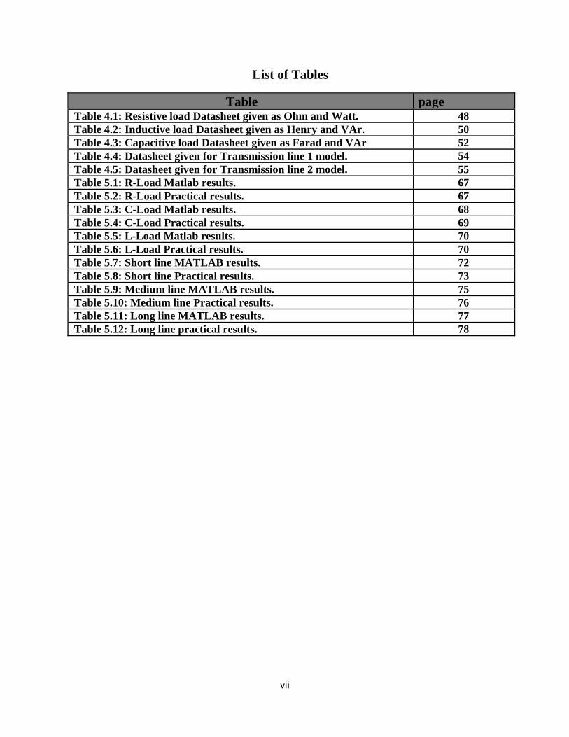
List of Tables

Table page

Table 4.1: Resistive load Datasheet given as Ohm and Watt. 48

Table 4.2: Inductive load Datasheet given as Henry and VAr. 50

Table 4.3: Capacitive load Datasheet given as Farad and VAr 52

Table 4.4: Datasheet given for Transmission line 1 model. 54

Table 4.5: Datasheet given for Transmission line 2 model. 55

Table 5.1: R-Load Matlab results. 67

Table 5.2: R-Load Practical results. 67

Table 5.3: C-Load Matlab results. 68

Table 5.4: C-Load Practical results. 69

Table 5.5: L-Load Matlab results. 70

Table 5.6: L-Load Practical results. 70

Table 5.7: Short line MATLAB results. 72

Table 5.8: Short line Practical results. 73

Table 5.9: Medium line MATLAB results. 75

Table 5.10: Medium line Practical results. 76

Table 5.11: Long line MATLAB results. 77

Table 5.12: Long line practical results. 78

1

Chapter One Introduction

1.1 Overview

1.2 Motivations

1.3 Objectives

1.4 Challenges

1.5 Importance

1.6 Time schedule

1.7 Expected results

2 | P a g e

1.1 Overview

The MATLAB/Simulink software is used to model and analyze the dynamic response of

various distribution components in form of smart grid lab at Palestine Polytechnic

University. The approach taken involves simulating each component stand alone, what will

be referred to as “Blocks”, where each block masks the mathematical and dynamic equations

of the individual components.

1.2 Motivation

The model will be validated with experimental data. A series of experiments will be

conducted on the smart grid system at the Renewable Energy Lab at the Electrical

Engineering Department PPU. The developed model will give more details about the effects

of the Embedded Generation (EG) unites and the Microturbines (MT) system on the

transmission and distribution systems. The model will be used to study the effects of

several factors such as the effects of EG and MT on the voltage profile, losses, harmonics,

and load flow profile.

1.3 Objectives

Recognize the electrical units used in the renewable energy laboratory and obtain

important information for each electrical unit.

Modeling each component of Smart grid system in the power lab at Palestine polytechnic

university using MATLAB/Simulink.

Make several practical experiments in energy laboratory located in PPU and compare the

results with the results we have obtained using MATLAB.

Develop a Smart grid Model for Education purposes.

3 | P a g e

1.4 Challenges

Limited knowledge of the MATLAB program due to lack of course education program

which has led to the self-learning.

Lack of case studies about our project.

Communications between each component in the smart grid is extremely important to

maximize the use of available electrical power in a reliable and cost effective way.

Therefore, how to efficiently manage the new, intelligent power system and integrate it

into the existing system has become one of the main challenges for the smart grid

infrastructure.

1.5 Importance

Develop a numerical Model for a smart grid system to be experimentally validated.

The Model will be developed for the educational purpose.

The Model will give more details about the system behavior and performance.

Make this project “LAB” as one of the requirements for Graduation, and name the

class as “Renewable energy lab”.

4 | P a g e

1.6 Time schedule

Task 1: Prepare the mathematical and dynamic equations necessary for the project to be modeled

and simulated using MATLAB software.

Task 2: Collection of datasheets for every module used in the project.

Task 3: Collection Data and information on the subject of the project.

Task 4: Simulate electrical units using MATLAB/Simulink according to the modules used in the

library at PPU.

Task 5: Finishing the graduation project book and make several practical experiments in energy

laboratory located in PPU.

Task 6: Prepare the presentation.

Week

Tasks

1 2 3 4 5 6 7 8 9 10 11 12 13 14 15 16

Task 1

Task 2

Task 3

Task 4

Task 5

Task 6

5 | P a g e

1.7 Expected outcomes

The modeling and simulation of distribution system components pertinent to a smart grid

was presented in this project. The components considered in this work included PV arrays,

with used Inverter module, Transmission lines, and Power measurements kit, several types

of three phase loads (R, L, and C), three phase induction machine implemented as wind

turbines simulator, and power circuit breaker. The methodology involves deriving the

equations of the components and creating modules in Simulink that mask the relevant

components equations.

2

6 | P a g e

Chapter Two Smart Grid Lab


2.1.1 Introduction



2.1.4 Line models

2.1.5 Three phase transformer & Supply unit.




2.2.3 Loads (R,L,C)


2.3.1 PV simulator module

2.4 Summary

7 | P a g e


2.1.1 Introduction

In this Chapter, a brief overview of all modules have been taken in the project to be modeled and

simulated using MATLAB/Simulink. Taking into account that all the information have been

taken from the modules used in the lab at Palestine Polytechnic University.

Smart grid lab consists of the following modules that will be simulated using MATLAB:

1) Power circuit breaker.

2) Maximum demand meter.

3) Line models.

4) Three phase transformer/Auto transformer.

5) Inverter grid.

6) Three phase induction machine.

7) PV simulator module.

8) Loads.

8 | P a g e


Three-phase power circuit breaker with normally closed

(DL 2108T02) or normally open (DL 2108T02A) auxiliary

contact. [1]

• Contact load capability: 400 Vac, 3 A.

• Supply voltage: single-phase from mains.

Power circuit breaker used for two operations: used to connect

or disconnect the contacts by using a specific control scheme

as shown on the module.

> ON button: to close the contacts.

> OFF button: to open the contacts.

SR flip flop used to achieve such a controlling procedure.

Figure 2.1: Power circuit breaker.


The power measurements module is a very

important module used a power analyzer for

many measurements, the procedure of

modeling and simulation of such module is

described later in chapter 3. [1]

• Input voltage: 500 V (max 800 Vrms).

• Input current: 5 A (max 20 Arms).

• Operating frequency: 47 ÷ 63 Hz.

• Auxiliary supply: single-phase from mains.

Figure 2.2: Maximum demand meter.

9 | P a g e

2.1.4 Line models

Two types of line models are used in the lab which represents:

1- Transmission line model.

2- Distribution line model.

Keeping in mind that line models can be used as three different types of lines: short, medium,

and long.

The functionality can be changed by connecting or disconnecting capacitors in parallel with

lines.

1) Transmission line model

Figure 2.3: Transmission line model.

Three-phase model of an overhead power transmission line 360 km long, voltage 380 kV and

current 1000 A. [1]

• Scale factor: 1:1000

Short line: is done by connecting the lower capacitors.

Medium line: is done by connecting the upper capacitors.

Long line: is done by connecting both upper and lower capacitors.

10 | P a g e

2) Distribution line model

Figure 2.4: Distribution line model.

Three‐phase model of an overhead power distribution line 110 km long, voltage 380 kV and

current 1000 A. [1]

• Scale factor: 1:1000

2.1.5 Three phase transformer & supply unit

Three phase transformer provides

voltage to transmission lines.

Primary

• 3 x 380 V windings with tap at 220 V

• Star or delta connection

Secondary

• 3 x 220 V windings.

• Star connection for 3 x 380 V

• Rated power: 800 VA

Figure 2.5: Three phase transformer. [1]

11 | P a g e

Figure 2.6: Three phase supply unit.

Three phase supply unit represents electrical power generation for both power plants and

renewable energies i.e. Wind turbines and PV cells.

Three phase supply unit provides mainly 5 outputs:

1) Three phase output voltage L1, L2, L3.

2) Protection earth PE.

3) Neutral N.

Datasheet: [1]

* 25A current operated earth leakage circuit breaker, sensitivity 30 mA.

* Three‐phase indicator lamps.

* Switch for simulation of wind or photovoltaic energy power source.

12 | P a g e



Figure 2.7: Inverter grid.

Inverter grid module uses a connection of many power electronic elements to be connected with

the PV cell to grid. The input to the inverter 12V from the PV source and provides ac voltage as

the datasheet as following: [1]

• Current max.: 30A

• Voltage: 12V

• Power: 360W

13 | P a g e


The following induction motor is implemented to be three phase induction generator by

connecting prime mover to the rotor to

simulate Wind turbine generation stage.

Datasheet: [1]

• Power: 1.5 kW

• Voltage: 220/380 V Δ/Y

• 4 poles

• Rated speed: 1500 rpm, 50 Hz

• Rated speed: 1800 rpm, 60 Hz

Figure 2.8: Three phase induction

machine.

2.2.3 Loads (R,L,C)

1) R load:

Datasheet: [1]

Single or three‐phase resistive

step‐variable load.

• Max. Power: 3 x 400 W

• Max. Voltage: 220/380 V Δ/Y

Figure 2.9: Resistive load.

14 | P a g e

2) L load:

Datasheet: [1]

Single or three‐phase inductive


• Max. Power: 3 x 300 VAR


Figure 2.10: Inductive load.

3) C load:

Datasheet: [1]

Single or three‐phase capacitive


• Max. Power: 3 x 275 VAR


Figure 2.11: Capacitive load.

15 | P a g e


2.3.1 PV simulator module

Photovoltaic simulator used for

measurement of the radiation and

It has a solar and a temperature

sensors.

Datasheet: [1]

Tilting photovoltaic module.

• Max. Power: 85 Watt.

• Max. Voltage: 12 Volt.

Figure 2.12: Photovoltaic simulator module.

16 | P a g e

2.3 Summary

A brief overview to the modules has been taken in this chapter in order to be

simulated later in chapter 3 & 4.

3

17 | P a g e

Chapter Three Modules Simulation 1

3.1 Smart grid modules modeling 3.1.1 Circuit breaker

3.1.2 Power Measurements


3.2.1 Harmonics 3.2.2 Linear and non-Linear loads 3.2.3 Power factor

3.3 Summary

18 | P a g e

3.1 Smart grid Modules modeling

This chapter contains circuit breaker and power measurements modules that designed

according to harmonic and power factor analysis with linear and non-linear loads.

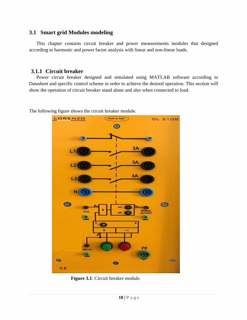
3.1.1 Circuit breaker Power circuit breaker designed and simulated using MATLAB software according to

Datasheet and specific control scheme in order to achieve the desired operation. This section will

show the operation of circuit breaker stand alone and also when connected to load.

The following figure shows the circuit breaker module.

Figure 3.1: Circuit breaker module.

19 | P a g e

Figure 3.2: Internal control scheme for Circuit Breaker.

The following figures show the circuit breaker module simulated using Simulink software in case

of ON and OFF operating states:

Figure 3.3: Circuit breaker ON state.

20 | P a g e

Figure 3.4: Circuit breaker OFF state.

The following figures show the simulation of circuit breaker module in case of ON and OFF

operating states when connected to three phase load:

Figure 3.5: Circuit breaker Simulation connected to three phase load.

21 | P a g e

Figure 3.6: ON and OFF circuit breaker output voltage simulation.

3.1.2 Power Measurements:

Power measurements designed and simulated using MATLAB software according to

Datasheet, harmonics, and power factor theories (described later in 3.2). In order to achieve the

desired operation, this section will show the operation of Power measurements stand alone and

also when connected to load and the inner content of simulated module.

The following figure shows the power measurements module and datasheet.

Microprocessor controlled three-phase power analyzer.

Measurement of voltages, currents, frequencies, active

Power, reactive power, apparent power, THD, power factor.

• Input voltage: 500 V (max 800 Vrms)

• Input current: 5 A (max 20 Arms)

• Operating frequency: 50Hz

Figure 3.7: Power measurement module.

22 | P a g e

Figure 3.8: Power measurement main block.

Figure 3.9: Inner content of power measurement main block.

23 | P a g e

Figure 3.10: Inside (figure 3.9) power measurement block.

The above Fig (3.10) consists of the following contents:

Phase A subsystem.

Phase B subsystem.

Phase C subsystem.

Three Phases subsystem.

Let’s Start with Phase A subsystem, since Phase B and C are the same construction except the

going and incoming flag signal, that can be shown in the next figure.

24 | P a g e

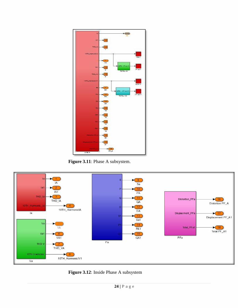
Figure 3.11: Phase A subsystem.

Figure 3.12: Inside Phase A subsystem

25 | P a g e

Phase A subsystem consist of the following subsystem blocks:

Figure 3.13: IA subsystem.

Figure 3.14: Inside IA subsystem.

26 | P a g e

IA subsystem consists of two subsystems.

1- Current subsystem.

Figure 3.15: Inside current subsystem.

2- Harmonic subsystem.

Figure 3.16: Inside Harmonic subsystem.

27 | P a g e

Figure 3.17: VA subsystem.

Figure 3.18: Inside VA subsystem.

VA subsystem consists also of two subsystems.

28 | P a g e

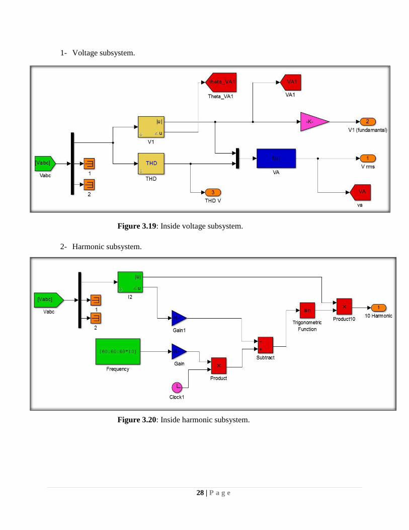
1- Voltage subsystem.

Figure 3.19: Inside voltage subsystem.

2- Harmonic subsystem.

Figure 3.20: Inside harmonic subsystem.

29 | P a g e

Figure 3.21: Phase A power subsystem (Pa).

Figure 3.22: Inside Pa subsystem.

30 | P a g e

PA subsystem consists of seven subsystems.

1- Apparent power subsystem.

Figure 3.23: Apparent Power subsystem.

2- Real power subsystem.

Figure 3.24: Real Power subsystem.

31 | P a g e

3- Reactive power subsystem.

Figure 3.25: Reactive power subsystem.

4- Distortion power subsystem.

Figure 3.26: Distortion power subsystem.

32 | P a g e

5- Fundamental apparent power.

Figure 3.27: Fundamental Apparent power subsystem.

6- Fundamental active power.

Figure 3.28: Fundamental active power subsystem.

33 | P a g e

7- Fundamental reactive power.

Figure 3.29: Fundamental reactive power subsystem.

Figure 3.30: Phase A power factor subsystem (PFa).

34 | P a g e

Figure 3.31: Inside PFa subsystem.

PFa subsystem consists of three subsystems.

1- Distortion power factor.

Figure 3.32: Distortion power factor subsystem.

35 | P a g e

2- Displacement power factor.

Figure 3.33: Displacement power factor subsystem.

3- Total power factor.

Figure 3.34: Total power factor subsystem.

And the above figures are the same as Phases B, and C.

36 | P a g e

Figure 3.35: Three phase subsystem.

Figure 3.36: Inside of Three phase subsystem.

37 | P a g e

The following figures show the simulation of power measurement module with and without

loading.

Figure 3.37: Simulation of power measurements module with multifunction.

Figure 3.38: Simulation of power measurements module connected to three-phase load.

And the next figure shows the power measurement simulation when connected to non-linear load.

38 | P a g e

Figure 3.39: Simulation of power measurements module connected to non-linear three-phase load.

Figure 3.40: First 10th order of harmonics current on phase A.

39 | P a g e

Figure 3.41: Combination modeling of Circuit Breaker and Power Measurement.


This section demonstrates harmonic, power factor, and (linear and non-linear loads) theories that

used in power measurements modeling using Simulink.

3.2.1 Harmonics: The deviation of the voltage and current waveforms from sinusoidal is described in terms of the

waveform distortion, often expressed as harmonic distortion.

Harmonics theory: A harmonic component in an AC power system is defined as a sinusoidal

component of a periodic waveform that has a frequency equal to an integer multiple of the

fundamental frequency of the system. Harmonics in voltage or current waveforms can then be

conceived as perfectly sinusoidal components of frequencies multiple of the fundamental

frequency: [2]

F (h) = (h) × (fundamental frequency) (3.1)

Where h is an integer

40 | P a g e

Figure 3.42: Shows an ideal 60-Hz waveform with a peak value of around 100 A.

Which can be taken as one per unit. Likewise, it also portrays waveforms of amplitudes (1/7),

(1/5), and (1/3) per unit and frequencies seven, five, and three times the fundamental frequency,

respectively. This behavior showing harmonic components of decreasing amplitude often

following an inverse law with harmonic order is typical in power system [2]

Figure 3.43: Ideal 60Hz waveform with harmonic components.

These waveforms can be expressed as:

i 1 = Im 1 sin ω t (3.2)

i 3 = Im 3 sin(3 ω t – δ 3 ) (3.3)

i 5 = Im 5 sin(5 ω t – δ 5 ) (3.4)

i 7 = Im 7 sin(7 ω t – δ 7 ) (3.5)

Where Imh is the peak RMS value of the harmonic current h . [2]

If we take only the first three harmonic components, the figure shows how a distorted current

waveform at the terminals of a six-pulse converter would look. There would be additional

41 | P a g e

harmonics that would impose a further distortion. The resultant distorted waveform can thus be

expressed as:

I total = Im 1 sin ω t + Im 3 sin(3 ω t – δ 3 ) + Im 5 sin(5 ω t – δ 5 ) + Im 7sin(7 ω t – δ 7)

(3.6)

In this way, a summation of perfectly sinusoidal waveforms can give rise to a distorted

waveform. Conversely, a distorted waveform can be represented as the superposition of a

fundamental frequency waveform with other waveforms of different harmonic frequencies and

amplitudes.

3.2.2 Linear and non-Linear loads: From the discussion in this section, it will be evident that a load that draws current from a

sinusoidal AC source presenting a waveform like that of Figure 3.43 cannot be conceived as a

linear load.

Linear loads:

Linear loads are those in which voltage and current signals follow one another very closely,

such as the voltage drop that develops across a constant resistance, which varies as a direct function

of the current that passes through it. This relation is better known as Ohm’s law and states that the

current through a resistance fed by a varying voltage source is equal to the relation between the

voltage and the resistance, as described by:

𝐼(𝑡) =𝑉(𝑡)

𝑅 (3.7)

This is why the voltage and current waveforms in electrical circuits with linear loads look alike.

Therefore, if the source is a clean open circuit voltage, the current waveform will look identical,

showing no distortion. Circuits with linear loads thus make it simple to calculate voltage and

current waveforms

42 | P a g e

Figure 3.44: Example for linear loads.

Non-Linear loads:

Nonlinear loads are loads in which the current waveform does not resemble the applied voltage

waveform due to a number of reasons, for example, the use of electronic switches that conduct

load current only during a fraction of the power frequency period.

Among the most common nonlinear loads in power systems are all types of rectifying devices like

those found in power converters, power sources, uninterruptible power supply (UPS) units, and

arc devices like electric furnaces and fluorescent lamps. Figure 3.45 provides a more extensive list

of various devices in this category.

Figure 3.45: Example for nonlinear loads.

43 | P a g e

3.2.3 Power factor:

Traditional methods of Power Factor Correction typically focus on displacement power factor

and therefore do not achieve the total energy savings available in facilities having both linear and

non–linear loads. Only through Total Power Factor Correction can the savings and power quality

be maximized.

When the loads are non–linear and the voltage is distorted the active, reactive and apparent power

cannot be calculated using traditional methods

The active power is the mean (or average) value of the instantaneous power. If the phase angles of

the voltage harmonics are neglected, the active power can be calculated as:

1

cos( )N

n n n

n

P V I

(3.8)

Now, the power factor can be calculated using equation

1

cos ( )N

n n n

n

V I

pfVI

(3.9)

But, the voltage rms value is a function of the total harmonic voltage distortion and the rms value

of the fundamental component of voltage:

2

1 1 VV V THD

(3.10)

And Therms value of current is a function of the total harmonic current distortion and the rms

value of the fundamental component of current

2

1 1 II I THD (3.11)

Using equations (3.11), (3.10) and (3.9), the power factor can be calculated as follows:

44 | P a g e

2 2

1

1

1 1I V

Ppf

S THD THD

(3.12)

There are two terms involved in the calculation of the power factor. The term 1

P

Sis the relationship

between the total active power (including harmonics) and the apparent fundamental power. This

term should not be called displacement power factor because it involves the active power caused

by the fundamental components and harmonics. The term

2 2

1

1 1I VTHD THD

Is the distortion power factor (PF dist), which depends on the

distortion of voltage and current. The power factor calculated as the product of the distortion power

factor and the proportion of the total active power to the fundamental apparent power is the total

power factor (TPF)

1

T dist

Ppf pf

S (3.13)

The term 1

P

S can be expressed as:

1 1 1 2

1 1 1

cos ( )cos

N

n n n

n

V IV IP

S S S

(3.14)

Where 1 1 1

1

cosV I

S

is the displacement power factor (

disppf ), so the total power factor can be

calculated as follows:

45 | P a g e

2

1

cos ( )N

n n n

nT disp dist

V I

pf pf pfS

(3.15)

In a similar way to the case of the non–linear loads and sinusoidal voltage, if the reactive power

of the loads increases, the displacement angle between the fundamental components of voltage

and current also increases and the total power factor decreases. If the distortion of current and

voltage increases the distortion power factor decreases and the total power factor decreases as well.

3.3 Summary

In this chapter a simulation is done for power circuit breakers and power measurements

modules using Simulink as blocks. The other modules will be simulated in chapter 4 same way as

this chapter in order to get all needed modules to be simulated and to study the behavior and

dynamic characteristics when connected together for educational purposes.

4

46 | P a g e

Chapter Four Modules Simulation 2

4.1 Loads and Transmission modules 4.1.1 Load modules



4.2.1 Dc-to-AC converter (inverter) 4.2.2 Buck-Boost converter 4.2.3 Maximum power point tracker 4.2.4 Filter


4.3.1 PV panel module 4.3.2 Three phase induction machine

4.4 Final Form

47 | P a g e

4.1 Loads and Transmission modules

4.1.1 Load modules In this section a simulation of loads modules and their Datasheets are shown in figure 4.1:

Figure 4.1: Three phase loads modules (R, L, and C).

1. Resistive load:

Figure 4.2: Three phase R load module.

48 | P a g e

Datasheet and the values of R (R1, R2, and R3) switches are shown: [6]

Table 4.1: Resistive load Datasheet given as Ohm and Watt.

Figure 4.3: Resistive load dialog box controlled values.

Position Resistance Max power per phase

1 1050 Ohm 46 W

2 750 Ohm 65 W

3 435 Ohm 110 W

4 300 Ohm 160 W

5 213 Ohm 230 W

6 150 Ohm 330 W

7 123 Ohm 400 W

49 | P a g e

Figure 4.4: Internal content of Resistive load module.

2. Inductive load:

Figure 4.5: Three phase L load module.

50 | P a g e

Datasheet and the values of L (L1, L2, and L3) switches are shown: [6]

Position Inductance Max power per phase

1 4.46 H 34 VAr

2 3.19 H 48 VAr

3 1.84 H 83 VAr

4 1.27 H 121 VAr

5 0.90 H 171 VAr

6 0.64 H 242 VAr

7 0.52 H 297 VAr

Table 4.2: Inductive load Datasheet given as Henry and VAr.

Figure 4.6: Inductive load dialog box controlled values.

51 | P a g e

Figure 4.7: Internal content of Inductive load module.

3. Capacitive load:

Figure 4.8: Three phase C load module.

52 | P a g e

Datasheet and the values of C (C1, C2, and C3) switches are shown: [6]

Position Capacitance Max power per phase

1 2 μF 30 VAr

2 3 μF 45 VAr

3 5 μF 76 VAr

4 7 μF 121 VAr

5 10 μF 152 VAr

6 13 μF 197 VAr

7 18 μF 275 VAr

Table 4.3: Capacitive load Datasheet given as Farad and VAr

Figure 4.9: Capacitive load dialog box controlled values.

53 | P a g e

Figure 4.10: Internal content of capacitive load module.


1. Transmission line model 1

This module is a three-phase model of an overhead power transmission line of 360 km, voltage

380 kV and current line 1000 A. The scale factor is 1:1000 for both, current and voltage so the

actual nominal values are 380 V and 1 A.[6]

Table 4.4 shows the Datasheet of Transmission line 1 used for simulation.

54 | P a g e

Resistance 13 Ω

Inductance 290 mH

Earth capacitance 1 μF

Mutual capacitance 0.5 μF

Earth return resistance 11 Ω

Earth return inductance 250 mH

Table 4.4: Datasheet given for Transmission line 1 model.[6]

Figure 4.11: Transmission line 360Km module.

The transmission line is presented as an equivalent “π” circuit with concentrated parameters. If

all the plugins are connected the capacitance value respect to neutral is 2.5 μF.

55 | P a g e

2. Transmission line model 2

This modulus is a three-phase model of an overhead power transmission line of 100 km, voltage

380 kV and current line 1000 A. The scale factor is 1:1000 for both, current and voltage so the

actual nominal values are 380 V and 1 A.

Table 4.5 shows the Datasheet of Transmission line 1 used for simulation.

Resistance 3.3 Ω

Inductance 80 mH

Earth capacitance 100 nF

Mutual capacitance 200 nF

Earth return resistance 3 Ω

Earth return inductance 69 mH

Table 4.5: Datasheet given for Transmission line 2 model. [6]

Figure 4.12: Transmission line 100Km module.

56 | P a g e

The transmission line is presented as an equivalent “π” circuit with concentrated parameters. If

all the plugins are connected the capacitance value respect to neutral is 500 nF.


4.2.1 Dc-to-AC converter( inverter)

Figure 4.13: DC to AC unit module.

Figure 4.14: DC to AC unit module in MATLAB.

57 | P a g e

Figure 4.15: Inside DC to AC unit module in MATLAB.[9]

The IGBTs are controlled by using pulse width modulation (PWM) technique.

4.2.2 Buck-Boost converter

Figure 4.16: Buck-Boost converter subsystem block.

Figure 4.17 shows the inner content of the buck-boost converter simulated using MATLAB.

58 | P a g e

Figure 4.17: Inside Buck-Boost converter subsystem block. [9]

4.2.3 Maximum power point tracker Figure 4.18 shows MPPT Controller subsystem simulated using Matlab.

Figure 4.18: MPPT controller subsystem block.

Figure 4.18: Inside MPPT controller subsystem block.

59 | P a g e

Due to fluctuations of Temperature and irradiation, the maximum power of PV panel needed to

be controlled using appropriate controller such as MPPT MPPT implementations utilize

algorithms that frequently sample panel voltages and currents, then adjust the duty ratio as

needed. Microcontrollers are employed to implement the algorithms.

The commonly used method to observe the maximum power point is called Perturb and

Observe (P&O).

Figure 4.19: Flowchart for P & O Algorithm. [10]

If the power increases then the perturbation is continued after the peak power is

reached the power at the MPP is zero.

After that the perturbation reverses the stable condition is arrived and algorithm

oscillates around the peak power point.

60 | P a g e

4.2.4 Filter A specific filter is used after the Inverter in order to get a pure sinusoidal output voltage.

Figure 4.20: Filter subsystem block.

Figure 4.21: Dialog box for Filter subsystem block.

Figure 4.22: Inside filter subsystem block.

61 | P a g e


4.3.1 PV panel module

Figure 4.23: PV panel subsystem block.

85W, 12V, full of cell for measurement of the radiation

It has a solar and a temperature sensor.

Figure 4.24: Inside PV panel subsystem block.

62 | P a g e


Three phase induction generator used to simulate Wind turbine generation stage. Figure 4.25

shows the induction machine inside MATLAB.

Figure 4.25: Three Phase induction machine. [6]

Figure 4.26: Inside three phase induction machine.

63 | P a g e

Dialog box Figure 4.27 used to enter the operating values for the induction machine.

Figure 4.27: Three phase induction machine dialog box.

64 | P a g e

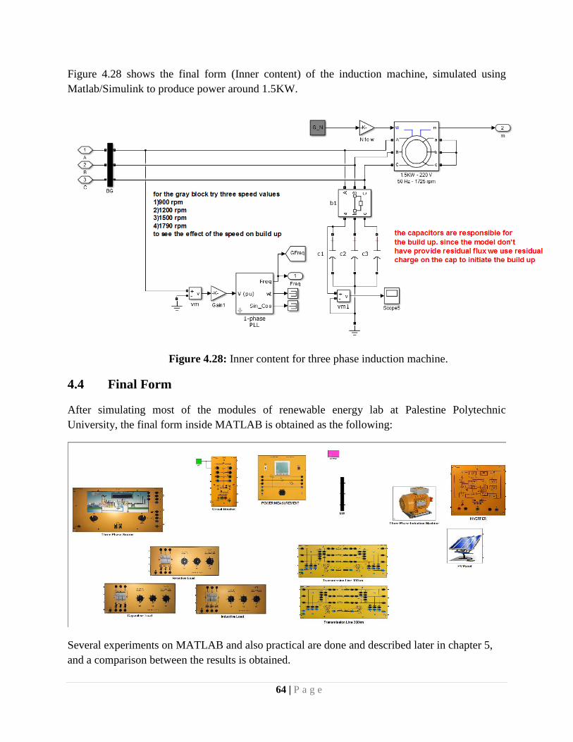
Figure 4.28 shows the final form (Inner content) of the induction machine, simulated using

Matlab/Simulink to produce power around 1.5KW.

Figure 4.28: Inner content for three phase induction machine.

4.4 Final Form

After simulating most of the modules of renewable energy lab at Palestine Polytechnic

University, the final form inside MATLAB is obtained as the following:

Several experiments on MATLAB and also practical are done and described later in chapter 5,

and a comparison between the results is obtained.

5

65 | P a g e

Chapter Five Experiments

5.1 Loads

5.1.1 Introduction

5.1.2 R-Load

5.1.3 C-Load

5.1.4 L-Load

5.2 Transmission

5.2.1 Short 5.2.2 Medium 5.2.3 Long

5.3 Results Validation 5.3.1 Load results


5.3.3 Validation check

5.4 Combined Loads

5.5 Conclusion

66 | P a g e

5.1 Loads

5.1.1 Introduction

In this chapter several experiments on MATLAB and also practical are done, and a

comparison between the results is obtained. After obtaining the comparison, a results validation

is done later in section 5.3.

5.1.2 R-Load

The objective of this experiment is to connect the electrical source with R-Load, and obtain

practical and experimental results. The connected electrical circuit will contain (Three phase

source, circuit breaker, Power measurements module, and Three phase R-Load module), as

shown in Figure 5.1.

Figure 5.1: R-Load experiment.

67 | P a g e

Tables 5.1 and 5.2 show the results obtained.

RLOAD

PF S Q P I V Position Resistance

1 50.8 0 50.8 0.22 230.9 1 1050 Ohm

1 71.11 0 71.11 0.308 230.9 2 750 Ohm

1 122.6 0 122.6 0.531 230.9 3 435 Ohm

1 177.8 0 177.8 0.77 230.9 4 300 Ohm

1 250.4 0 250.4 1.084 230.9 5 213 Ohm

1 355.5 0 355.5 1.54 230.9 6 150 Ohm

1 433.6 0 433.6 1.877 230.9 7 123 Ohm Table 5.1: R-Load Matlab results.

R-LOAD


1 50 0 50 0.21 231 1 1050 Ohm

1 70 0 70 0.3 229.5 2 750 Ohm

1 120 0 120 0.52 228.8 3 435 Ohm

1 180 0 180 0.77 228.5 4 300 Ohm

1 251 0 251 1.08 228 5 213 Ohm

1 355 0 355 1.5 228 6 150 Ohm

1 425 0 425 1.8 228 7 123 Ohm Table 5.2: R-Load Practical results.

68 | P a g e

5.1.3 C-Load

The connected electrical circuit will contain (Three phase source, circuit breaker, Power

measurements module, and Three phase C-Load module), as shown in Figure 5.2.

Figure 5.2: C-Load experiment.


C-LOAD

PF S Q P I V Position Capacitance

0 33.53 -33.5 0 0.145 230.9 1 2 μF

0 50.27 -50.27 0 0.217 230.9 2 3 μF

0 83.78 -83.78 0 0.363 230.9 3 5 μF

0 117.3 -117.3 0 0.508 230.9 4 7 μF

0 167.6 -167.6 0 0.725 230.9 5 10 μF

0 217.8 -217.8 0 0.943 230.9 6 13 μF

0 301.6 -301.6 0 1.306 230.9 7 18 μF Table 5.3: C-Load Matlab results.

69 | P a g e

C-LOAD

PF S Q P I V Position Capacitance

0 30 -30 0 0.15 231 1 2 μF

0 50 -50 0 0.22 229.5 2 3 μF

0 80 -80 0 0.36 228.8 3 5 μF

0 130 -130 0 0.59 228.5 4 7 μF

0 160 -160 0 0.74 228 5 10 μF

0 210 -210 0 0.97 228 6 13 μF

0 290 -290 0 1.33 228 7 18 μF Table 5.4: C-Load Practical results.

5.1.4 L-Load

The connected electrical circuit will contain (Three phase source, circuit breaker, Power

measurements module, and Three phase L-Load module), as shown in Figure 5.3.

Figure 5.3: L-Load experiment.

70 | P a g e


L-LOAD

PF S Q P I V Position Inductance

0 38.06 38.06 0 0.165 230.9 1 4.46 H

0 53.22 53.22 0 0.23 230.9 2 3.19 H

0 92.26 92.26 0 0.399 230.9 3 1.84 H

0 133.7 133.7 0 0.578 230.9 4 1.27 H

0 188.6 188.6 0 0.817 230.9 5 0.90 H

0 265.2 265.2 0 1.149 230.9 6 0.64 H

0 326.5 326.5 0 1.414 230.9 7 0.52 H Table 5.5: L-Load Matlab results.

L-LOAD

PF S Q P I V Position Inductance

0 38 38 0 0.16 231 1 4.46 H

0 53 53 0 0.23 229.5 2 3.19 H

0 91 91 0 0.4 228.8 3 1.84 H

0 134 134 0 0.55 228.5 4 1.27 H

0 190 190 0 0.83 228 5 0.90 H

0 273 273 0 1.19 228 6 0.64 H

0 333 333 0 1.44 228 7 0.52 H Table 5.6: L-Load Practical results.

71 | P a g e

5.2 Transmission

5.2.1 Short

To connect the transmission line module as short line the capacitors between lines and

neutral must be connected.

The connected electrical circuit will contain (Three phase source, circuit breaker, 2 Power

measurement modules, 100Km Transmission line, and Three phase R-Load module), as shown

in Figure 5.4.

Figure 5.4: Transmission line connected as short experiment.

72 | P a g e


R-LOAD /Short

Supply (Sending) Side


0.9944 51.3 -5.4 51 0.222 230.9 1 1050 Ohm

0.9982 71.5 -4.3 71.4 0.309 230.9 2 750 Ohm

1 122 0.3 122 0.528 230.9 3 435 Ohm

0.999 176 7.9 175.6 0.76 230.9 4 300 Ohm

0.996 245 21.8 244.3 1.062 230.9 5 213 Ohm

0.9897 344 49.23 340 1.488 230.9 6 150 Ohm

0.9836 414 74.64 407.5 1.794 230.9 7 123 Ohm

Load (Receiving) Side


1 50.6 0 50.6 0.219 230.5 1 1050 Ohm

1 70.6 0 70.62 0.307 230.1 2 750 Ohm

1 121 0 120.7 0.527 229.2 3 435 Ohm

1 173 0 173.2 0.76 228 4 300 Ohm

1 240 0 240.2 1.062 226.2 5 213 Ohm

1 323 0 323.3 1.488 223.3 6 150 Ohm

1 396 0 396.4 1.795 220.8 7 123 Ohm

Table 5.7: Short line MATLAB results.

73 | P a g e

R-LOAD /Short



1 50 0 50 0.216 231 1 1050 Ohm

1 70 0 70 0.302 231 2 750 Ohm

1 117 0 117 0.51 231 3 435 Ohm

0.999 171.14321 7 171 0.746 230.2 4 300 Ohm

0.996 234.85315 20 234 1.016 229 5 213 Ohm

0.991 326.84094 43 324 1.438 230.7 6 150 Ohm

0.987 387.98582 62 383 1.694 230.2 7 123 Ohm

Load (receiving) Side


1 49 0 49 0.214 229.1 1 1050 Ohm

1 69 0 69 0.302 228.8 2 750 Ohm

1 115 0 115 0.51 226.5 3 435 Ohm

1 167 0 167 0.746 224.1 4 300 Ohm

1 226 0 226 1.022 220.2 5 213 Ohm

1 305 0 305 1.426 216 6 150 Ohm

1 356 0 356 1.686 214.2 7 123 Ohm

Table 5.8: Short line Practical results.

74 | P a g e

5.2.2 Medium

To connect the transmission line module as medium line the capacitors between lines must

be connected. The connected electrical circuit will contain (Three phase source, circuit breaker, 2

Power measurement modules, 100Km Transmission line, and Three phase R-Load module), as


Figure 5.5: Transmission line connected as medium experiment.


R-LOAD /Medium



0.9854 51.7 -8.816 50.95 0.224 230.9 1 1050 Ohm

0.9943 71.6 -7.642 71.16 0.31 230.9 2 750 Ohm

0.9997 122 -2.98 121.9 0.528 230.9 3 435 Ohm

0.9997 176 4.62 175.5 0.76 230.9 4 300 Ohm

0.9971 245 18.55 244.4 1.062 230.9 5 213 Ohm

0.991 343 46.05 340.3 1.487 230.9 6 150 Ohm

0.985 414 71.52 407.9 1.793 230.9 7 123 Ohm

75 | P a g e



1 50.7 0 50.68 0.219 230.7 1 1050 Ohm

1 70.7 0 70.73 0.307 230.3 2 750 Ohm

1 121 0 120.9 0.527 229.3 3 435 Ohm

1 174 0 173.5 0.76 228.1 4 300 Ohm

1 241 0 240.6 1.063 226.4 5 213 Ohm

1 333 0 332.8 1.489 223.4 6 150 Ohm

1 397 0 397 1.797 221 7 123 Ohm

Table 5.9: Medium line MATLAB results.

R-LOAD /Medium



1 49 0 49 0.218 230 1 1050 Ohm

1 69 0 69 0.306 229.2 2 750 Ohm

1 117 0 117 0.512 229.1 3 435 Ohm

1 171.04678 4 171 0.742 228.8 4 300 Ohm

0.998 234.54637 16 234 1.022 229 5 213 Ohm

0.992 322.49031 40 320 1.424 228.5 6 150 Ohm

0.989 384.40083 58 380 1.682 228 7 123 Ohm

76 | P a g e



1 48 0 48 0.212 228 1 1050 Ohm

1 67 0 67 0.298 225.2 2 750 Ohm

1 112 0 112 0.502 222.8 3 435 Ohm

1 163 0 163 0.734 220 4 300 Ohm

1 223 0 223 1.018 218 5 213 Ohm

1 303 0 303 1.416 215 6 150 Ohm

1 354 0 354 1.676 214 7 123 Ohm

Table 5.10: Medium line Practical results.

5.2.3 Long

To connect the transmission line module as long line the upper and lower capacitors are

connected. The connected electrical circuit will contain (Three phase source, circuit breaker, 2

Power measurement modules, 100Km Transmission line, and Three phase R-Load module), as


Figure 5.6: Transmission line connected as long experiment.

77 | P a g e


R-LOAD /Long



0.9568 53.4 -15.51 51.05 0.231 230.9 1 1050 Ohm

0.9804 72.7 -14.33 71.28 0.315 230.9 2 750 Ohm

0.9969 123 -9.625 122.2 0.531 230.9 3 435 Ohm

0.9999 176 -1.968 176 0.762 230.9 4 300 Ohm

0.9988 245 12.05 245.1 1.063 230.9 5 213 Ohm

0.9933 344 39.71 341.2 1.487 230.9 6 150 Ohm

0.9875 414 65.31 409 1.793 230.9 7 123 Ohm



1 50.8 0 50.84 0.22 231 1 1050 Ohm

1 71 0 70.96 0.307 230.7 2 750 Ohm

1 121 0 121.3 0.528 229.7 3 435 Ohm

1 174 0 174 0.762 228.5 4 300 Ohm

1 241 0 241.3 1.064 226.7 5 213 Ohm

1 334 0 333.8 1.492 223.8 6 150 Ohm

1 398 0 398.2 1.799 221.3 7 123 Ohm

Table 5.11: Long line MATLAB results.

78 | P a g e

R-LOAD /Long



0.964 52.886671 -14 51 0.23 231 1 1050 Ohm

0.985 71.09749 -12.44 70 0.312 230 2 750 Ohm

0.997 119.35618 -9.214 119 0.52 230 3 435 Ohm

0.996 172.65283 -15 172 0.744 229 4 300 Ohm

0.999 234.21358 10 234 1.024 228.6 5 213 Ohm

0.995 328.76283 34 327 1.436 228.2 6 150 Ohm

0.991 389.48684 52 386 1.694 228 7 123 Ohm



1 49 0 49 0.214 228 1 1050 Ohm

1 68 0 68 0.3 227.6 2 750 Ohm

1 113 0 113 0.508 223.2 3 435 Ohm

1 164 0 164 0.738 222 4 300 Ohm

1 223 0 223 1.016 217.4 5 213 Ohm

1 305 0 305 1.424 213 6 150 Ohm

1 358 0 358 1.68 211.7 7 123 Ohm

Table 5.12: Long line practical results.

79 | P a g e

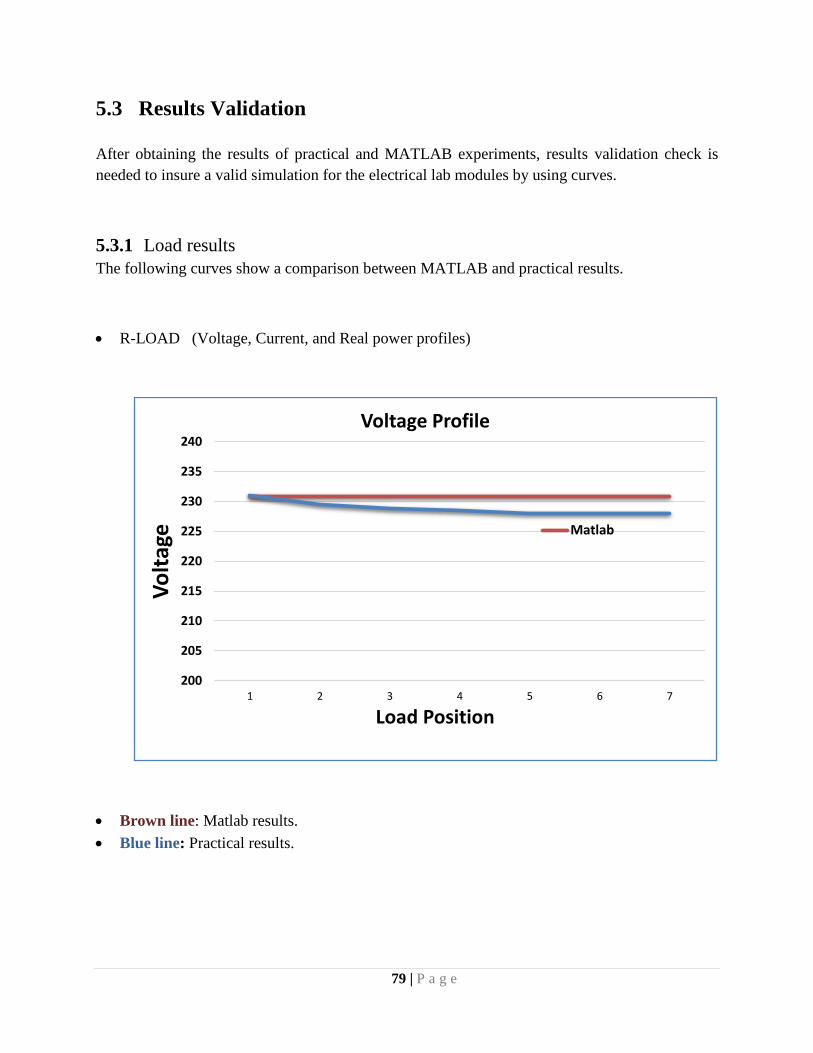
5.3 Results Validation

After obtaining the results of practical and MATLAB experiments, results validation check is

needed to insure a valid simulation for the electrical lab modules by using curves.

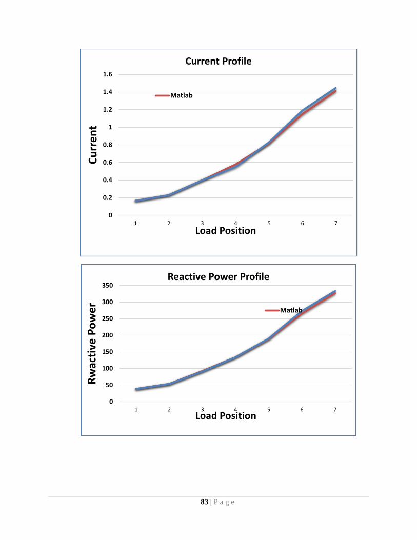
5.3.1 Load results

The following curves show a comparison between MATLAB and practical results.

R-LOAD (Voltage, Current, and Real power profiles)

Brown line: Matlab results.

Blue line: Practical results.

200

205

210

215

220

225

230

235

240

1 2 3 4 5 6 7

Vo

ltag

e

Load Position

Voltage Profile

Matlab

80 | P a g e

0

0.2

0.4

0.6

0.8

1

1.2

1.4

1.6

1.8

2

1 2 3 4 5 6 7

Cu

rre

nt

Load Position

Current Profile

Matlab

0

50

100

150

200

250

300

350

400

450

500

1 2 3 4 5 6 7

Po

we

r

Load Position

Power Profile

Matlab

81 | P a g e

C-LOAD (Voltage, Current, and Reactive power profiles)

200

205

210

215

220

225

230

235

240

1 2 3 4 5 6 7

Vo

ltag

e

Load Position

Voltage Profile

Matlab

0

0.2

0.4

0.6

0.8

1

1.2

1.4

1.6

1 2 3 4 5 6 7

Cu

rre

nt

Load Position

Current Profile

Matlab

82 | P a g e

L-LOAD (Voltage, Current, and Reactive power profiles)

-350

-300

-250

-200

-150

-100

-50

01 2 3 4 5 6 7

Re

acti

ve P

ow

er

Load Position

Reactive Power Profile

Matlab

200

205

210

215

220

225

230

235

240

1 2 3 4 5 6 7

Vo

ltag

e

Load Position

Voltage Profile

Matlab

83 | P a g e

0

0.2

0.4

0.6

0.8

1

1.2

1.4

1.6

1 2 3 4 5 6 7

Cu

rre

nt

Load Position

Current Profile

Matlab

0

50

100

150

200

250

300

350

1 2 3 4 5 6 7

Rw

acti

ve P

ow

er

Load Position

Reactive Power Profile

Matlab

84 | P a g e


Short Line (Voltage, Current, Real power, Reactive power, and Apparent power profiles)

200202204206208210212214216218220222224226228230232234236238240

1 2 3 4 5 6 7

Vo

ltag

e

Load Position

Voltage Profile

Matlab_S Experimental_S Matlab_R Experimental_R

0

0.2

0.4

0.6

0.8

1

1.2

1.4

1.6

1.8

2

1 2 3 4 5 6 7

Cu

rre

nt

Load Position

Current Profile


85 | P a g e

-10

0

10

20

30

40

50

60

70

80

1 2 3 4 5 6 7

Rw

acti

ve P

ow

er

Load Position

Rwactive Power Profile

Matlab_S Experimental_S

0

50

100

150

200

250

300

350

400

450

1 2 3 4 5 6 7

Cu

rre

nt

Load Position

Power Profile


86 | P a g e

Medium Line (Voltage, Current, Real power, Reactive power, and Apparent power profiles)

0

50

100

150

200

250

300

350

400

450

1 2 3 4 5 6 7

Ap

par

en

t P

ow

er

Load Position

Apparent Power Profile


200202204206208210212214216218220222224226228230232234236238240

1 2 3 4 5 6 7

Vo

ltag

e

Load Position

Voltage Profile


87 | P a g e

0

0.2

0.4

0.6

0.8

1

1.2

1.4

1.6

1.8

2

1 2 3 4 5 6 7

Cu

rre

nt

Load Position

Current Profile


-20

-10

0

10

20

30

40

50

60

70

80

1 2 3 4 5 6 7

Rw

acti

ve P

ow

er

Load Position



88 | P a g e

0

50

100

150

200

250

300

350

400

450

1 2 3 4 5 6 7

Cu

rren

t

Load Position

Power Profile


0

50

100

150

200

250

300

350

400

450

1 2 3 4 5 6 7

Ap

par

en

t P

ow

er

Load Position



89 | P a g e

Long Line (Voltage, Current, Real power, Reactive power, and Apparent power profiles)

200202204206208210212214216218220222224226228230232234236238240

1 2 3 4 5 6 7

Vo

lta

ge

Load Position

Voltage Profile


0

0.2

0.4

0.6

0.8

1

1.2

1.4

1.6

1.8

2

1 2 3 4 5 6 7

Cu

rren

t

Load Position

Current Profile


90 | P a g e

-20

-10

0

10

20

30

40

50

60

70

1 2 3 4 5 6 7

Rw

acti

ve P

ow

er

Load Position



0

50

100

150

200

250

300

350

400

450

1 2 3 4 5 6 7 8

Cu

rre

nt

Load Position

Power Profile


91 | P a g e

5.3.3 Validation Check

Validation check is done by finding the maximum deviation between Practical and

MATLAB results, and also by finding the max error.

MAX value = 𝐴𝑏𝑠𝑜𝑙𝑢𝑡𝑒 𝑣𝑎𝑙𝑢𝑒 𝑜𝑓 (𝑃𝑟𝑎𝑐𝑡𝑖𝑐𝑎𝑙 − 𝑀𝐴𝑇𝐿𝐴𝐵).

MAX error = 𝑀𝐴𝑋 𝐷𝑒𝑣𝑖𝑎𝑡𝑖𝑜𝑛

𝑀𝐴𝑋 𝑣𝑎𝑙𝑢𝑒 * 100%.

Accuracy % = 100- MAX error.

So, by using the up-mentioned three methods, a validation accuracy is obtained.

0

50

100

150

200

250

300

350

400

450

1 2 3 4 5 6 7

Ap

par

en

t P

ow

er

Load Position



92 | P a g e

Loads:

Validation Accuracy for R-Load:

Validation Accuracy for C-Load:

pf S Q P I V C

0 3.53 3.5 0 0.003 0.1 1

0 0.27 0.27 0 0.001 1.4 2

0 3.78 3.78 0 0.001 2.1 3

0 12.7 12.7 0 0.08 2.4 4

0 7.6 7.6 0 0.013 2.9 5

0 7.8 7.8 0 0.023 2.9 6

0 11.6 11.6 0 0.028 2.9 7

0 12.7 12.7 0 0.08 2.9 MAX deviation

0 4.211 4.211 0 6.126 1.25595 MAX error

- 95.79 95.79 - 93.87 98.744 Accuracy %

pf S Q P I V R

0 0.8 0 0.8 0.006 0.1 1

0 1.11 0 1.11 0.004 1.4 2

0 2.6 0 2.6 0.015 2.1 3

0 2.2 0 2.2 0 2.4 4

0 0.6 0 0.6 0.006 2.9 5

0 0.5 0 0.5 0.04 2.9 6

0 8.6 0 8.6 0.077 2.9 7

0 8.6 0 8.6 0.077 2.9 MAX deviation

0 1.983 0 1.983 4.102 1.25595 MAX error

- 98.02 - 98.02 95.9 98.744 Accuracy %

93 | P a g e

Validation Accuracy for L-Load:

pf S Q P I V L

0 0.06 0.06 0 0.001 0.1 1

0 0.22 0.22 0 0 1.4 2

0 1.26 1.26 0 0.001 2.1 3

0 0.3 0.3 0 0.03 2.4 4

0 1.4 1.4 0 0.009 2.9 5

0 7.8 7.8 0 0.039 2.9 6

0 6.5 6.5 0 0.03 2.9 7

0 7.8 7.8 0 0.039 2.9 MAX deviation

0 2.389 2.389 0 2.758 1.25595 MAX error

- 97.61 97.61 - 97.24 98.744 Accuracy %

Transmission:

Validation Accuracy for R-Load at Sending side:

S Q P I V R

1.036 0.4 1 0.006 0.1 1

1.456 1.1 1.4 0.007 0.1 2

5 0.3 5 0.018 0.1 3

4.634 0.9 4.6 0.014 0.7 4

10.42 1.8 10.3 0.046 1.9 5

16.7 6.23 16 0.05 0.2 6

26.29 12.64 24.5 0.1 0.7 7

26.29 12.64 24.5 0.1 1.9 MAX deviation

6.347 16.93 6.012 5.574 0.823 MAX error

93.65 83.07 93.99 94.43 99.18 Accuracy %

94 | P a g e

Validation Accuracy for R-Load at Receiving side:

S Q P I V R

1.6 0 1.6 0.005 1.4 1

1.62 0 1.62 0.005 1.3 2

5.7 0 5.7 0.017 2.7 3

6.2 0 6.2 0.014 3.9 4

14.2 0 14.2 0.04 6 5

18.3 0 18.3 0.062 7.3 6

40.4 0 40.4 0.109 6.6 7

40.4 0 40.4 0.109 7.3 MAX deviation

10.19 0 10.19 6.072 3.167 MAX error

89.81 - 89.81 93.93 96.83 Accuracy %

Validation Accuracy for C-Load at Sending side:

S Q P I V C

2.136 1.316 1.95 0.006 0.9 1

2.213 0.622 2.16 0.004 1.7 2

4.898 0.02 4.9 0.016 1.8 3

4.514 0.62 4.5 0.018 2.1 4

10.56 2.55 10.4 0.04 1.9 5

20.91 6.05 20.3 0.063 2.4 6

29.72 13.52 27.9 0.111 2.9 7

29.72 13.52 27.9 0.111 2.9 MAX deviation

7.177 18.9 6.84 6.191 1.256 MAX error

92.82 81.1 93.16 93.81 98.74 Accuracy %

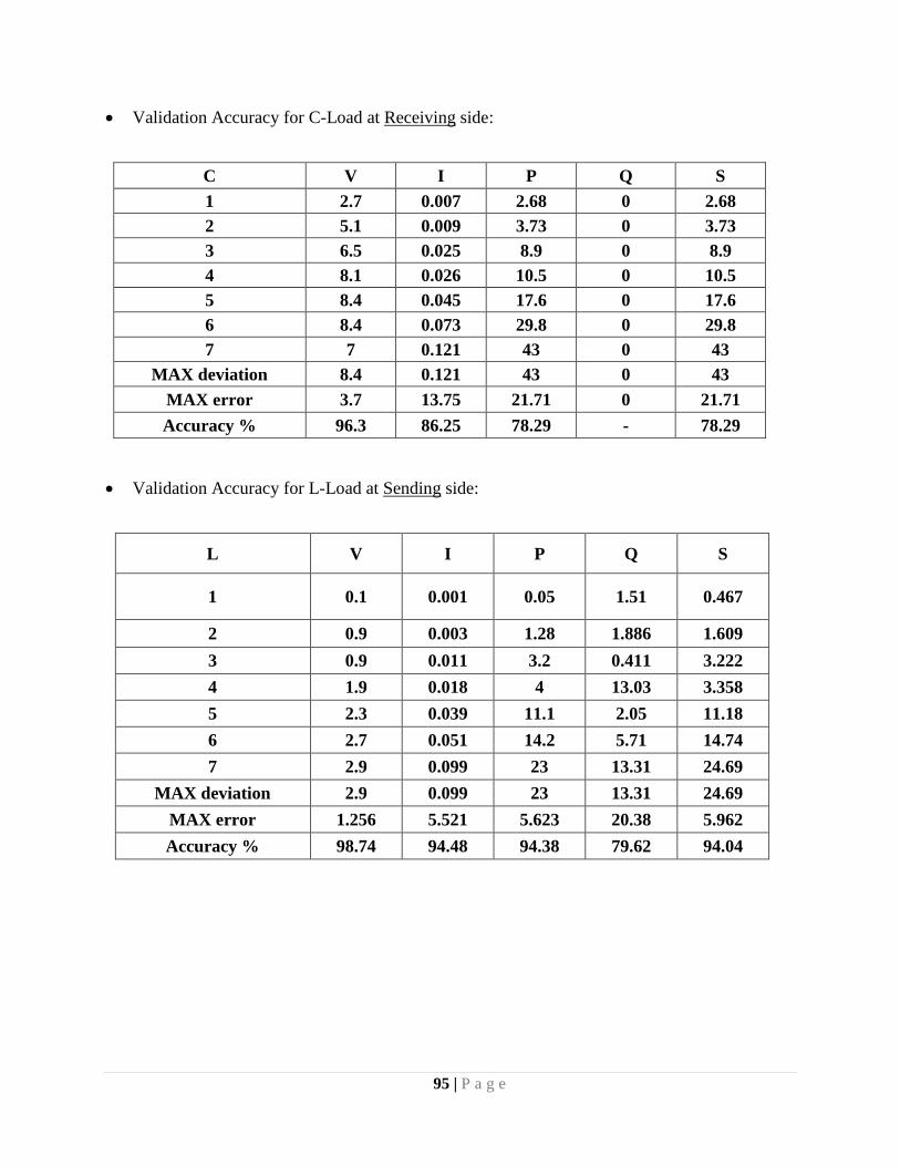
95 | P a g e

Validation Accuracy for C-Load at Receiving side:

S Q P I V C

2.68 0 2.68 0.007 2.7 1

3.73 0 3.73 0.009 5.1 2

8.9 0 8.9 0.025 6.5 3

10.5 0 10.5 0.026 8.1 4

17.6 0 17.6 0.045 8.4 5

29.8 0 29.8 0.073 8.4 6

43 0 43 0.121 7 7

43 0 43 0.121 8.4 MAX deviation

21.71 0 21.71 13.75 3.7 MAX error

78.29 - 78.29 86.25 96.3 Accuracy %

Validation Accuracy for L-Load at Sending side:

S Q P I V L

0.467 1.51 0.05 0.001 0.1 1

1.609 1.886 1.28 0.003 0.9 2

3.222 0.411 3.2 0.011 0.9 3

3.358 13.03 4 0.018 1.9 4

11.18 2.05 11.1 0.039 2.3 5

14.74 5.71 14.2 0.051 2.7 6

24.69 13.31 23 0.099 2.9 7

24.69 13.31 23 0.099 2.9 MAX deviation

5.962 20.38 5.623 5.521 1.256 MAX error

94.04 79.62 94.38 94.48 98.74 Accuracy %

96 | P a g e

Validation Accuracy for L-Load at Receiving side:

S Q P I V L

1.84 0 1.84 0.006 3 1

2.96 0 2.96 0.007 3.1 2

8.3 0 8.3 0.02 6.5 3

10 0 10 0.024 6.5 4

18.3 0 18.3 0.048 9.3 5

28.8 0 28.8 0.068 10.8 6

40.2 0 40.2 0.119 9.6 7

40.2 0 40.2 0.119 10.8 MAX deviation

10.09543 0 10.09543 6.614786 4.675325 MAX error

89.9 - 89.9 93.39 95.32 Accuracy %

For the Accuracy% results obtained by loads and Transmission experiments indicate to good

results, and therefore the Simulation for renewable energy lab at PPU has succeeded.

5.4 Combined Loads

In this section, several combined loads experiments have been made on MATLAB/Simulink

environment.

Experiment# 1:

Figure 5.7: RLC combined load experiment.

97 | P a g e

Figure 5.8: RLC combined load experiment metering results.

Experiment# 2:

Figure 5.9: RC combined load with transmission experiment.

98 | P a g e

Figure 5.10: RC combined load with transmission experiment results.

Experiment# 3:

Figure 5.11: RL combined load with transmission experiment.

99 | P a g e

Figure 5.12: RL combined load with transmission experiment results.

5.5 Conclusion

The objective was mainly about deriving the equations of the components to be simulated using

MATLAB/Simulink, in order to create modules/Blocks in Simulink to study the behavior of the

system components under different operating conditions. The modules used for the simulation

were (Power circuit breaker, Maximum demand meter, PV module, three phase induction

generator, Loads, Transmission lines, and Inverter module).

Bibliography

1

[1] 1360319989-DL SGWD – SMARTGRID [2] Technical Application Papers No.8 Power factor correction and harmonic filtering in electrical plants.

[3] H. S. Rauschenbach, Solar Cell Array Design Handbook. New York: Van Nostrand Reinhold, 1980.

[4] D. Sera, R. Teodorescu, and P. Rodriguez, ―PV panel model based on datasheet values,‖ in Proc. IEEE

Int. Symp. Ind. Electron. (ISIE), 2007, pp. 2392–2396.

[5] W. De Soto, S.A. Klein, and W. A. Beckman, ―Improvement and validation of a model for

photovoltaic array performance,‖ Solar Energy, vol. 80, no. 1, pp. 78–88, Jan. 2006.

[6] delorenzoglobal.com/en/laboratori/smartgrid/catalogo.php?sez=food&id=401&albero=0.1

[12] N. Mohan, T.M. Undeland, and W.P. Robbins. Power Electronics: Converters, Applications, and

Design Second Edition, John Wiley, 1995.

[7] EXPERIMENTAL CONCEPTS OF SMART GRID TECHNOLOGY BASED ON DELORENZO SMART GRID .Dr.

Pedro Ponce & Dr. Arturo Molina

[8] KC200GT High Efficiency Multicrystal Photovoltaic Module Datasheet Kyocera. [Online]. Available: http://www.kyocera.com.sg/products/solar/pdf/kc200gt.pdf [9] H. Sira-Ramírez and R. Silva-Ortigoza. Control Design Techniques in Power Electronics Devices, Springer, 2006. [10] MAXIMUM POWER POINT TRACKING IN PHOTOVOLTAIC SYSTEMS by ;Qinhao Zhang B.S., Shanghai Jiao Tong University, China, 2011

palestine polytechnic university college of engineering

Documents