panda manual

PANDA Manual

Zaixu Cui & Suyu Zhong & Gaolang Gong National Key Laboratory of Cognitive Neuroscience and Learning

Beijing Normal University, China

• Overview • Setup• Files/Directories selection• Preparing raw data• Setting inputs & outputs • Changing parameters • Initiating process• Monitoring progress • Understanding resultant files• Utilities

2

Contents

Overview

3

Linux OS (Ubuntu)Matlab (2010b) FSL (4.1.6) PSOM (0.9) Diffusion Toolkit (0.6.2)MRIcron (dcm2nii)

Development Environment:

OverviewAdvantage of PANDA

4

Automatic: Fully-automatic processing from DICOM/NIfTI files to ready-for-statistic data at multiple levels (Atlas-level, Voxel-level, and TBSS-level), brain anatomical networks (deterministic and probabilistic) constructed by using diffusion tractography for any number of subjects.

Parallel: Running jobs in parallel using multiple CPUs of one single computer or within a distributed computing environment.

Smart: If the program terminates mid-way, you can load configuration file and click ‘RUN’, then PANDA will restart from the terminate point. If you change some options, PANDA will only restart the procedure related to these options.

Hidden: The jobs will be run in background, and PANDA & Matlab can be even closed.

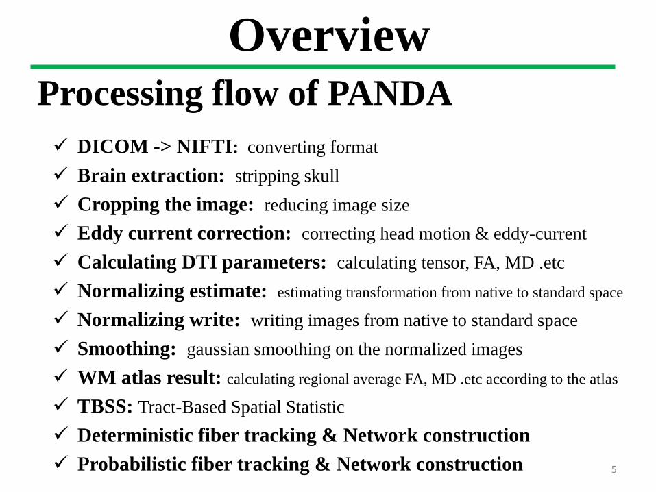
OverviewProcessing flow of PANDA

5

DICOM -> NIFTI: converting format Brain extraction: stripping skull Cropping the image: reducing image size Eddy current correction: correcting head motion & eddy-current Calculating DTI parameters: calculating tensor, FA, MD .etc Normalizing estimate: estimating transformation from native to standard space

Normalizing write: writing images from native to standard space Smoothing: gaussian smoothing on the normalized images WM atlas result: calculating regional average FA, MD .etc according to the atlas

TBSS: Tract-Based Spatial Statistic Deterministic fiber tracking & Network construction Probabilistic fiber tracking & Network construction

6

Overview

6

AssociationsFSL

Diffusion data was processed mainly using FSL commands.http://www.fmrib.ox.ac.uk/fsl/

Diffusion ToolkitFor deterministic fiber tracking.http://www.trackvis.org/dtk/

MRIcron (dcm2nii)For converting DICOM to NIfTI.http://www.mccauslandcenter.sc.edu/mricro/mricron

7

Overview

7

AssociationsPSOMThe pipeline system for Octave and Matlab (PSOM) is a lightweight library to manage complex multi-stage data processing. A pipeline is a collection of jobs, i.e. Matlab or Octave codes with a well identified set of options that are using files for inputs and outputs.PSOM can automatically offer the following services:Run jobs in parallel using multiple CPUs or within a distributed computing environment.Generate log files and keep track of the pipeline execution. These logs are detailed enough to fully reproduce the analysis.Handle job failures : successful completion of jobs is checked and failed jobs can be restarted.Handle updates of the pipeline : change options or add jobs and let PSOM figure out what to reprocess !http://code.google.com/p/psom/

• Overview • Setup• Files/Directories selection • Preparing raw data• Setting inputs & outputs • Changing parameters • Save configuration & Initiating process• Monitoring progress • Understanding resultant files• Utilities

8

Contents

SetupRequirements :

Linux OS / MACPANDA has been tested in Linux (Ubuntu, Centos, Fedora)

and MAC

Matlab

FSL

9

Now, PANDA is only available for /bin/sh, /bin/bash, /bin/ksh Now.We will make it available for /bin/tcsh, /bin/csh in next version.

SetupFSL Setup :

10

If FSL has not been installed, PANDA can’t be opened and a message box will appear.

Download and install FSL:http://www.fmrib.ox.ac.uk/fsl/fsl/downloading.html

SetupFSL Download :

11

Linux OS:Please download Linux Centos version FSL in FSL

download page, don’t download Linux Ubuntu/Debianversion FSL.

PANDA will not work well with Ubuntu/Debianversion FSL.

MAC OS:Please download MAC version FSL

SetupPANDA in MAC OS:

Input this command in terminal first:sudo launchctl load -w /System/Library/LaunchDaemons/com.apple.atrun.plist

Then, PANDA will work well in MAC.

SetupDownload & Unzip:

13

Download PANDA:http://www.nitrc.org/projects/panda/

Unzip:Example: Unzip PANDA-1.1.0_32.tar.gz

tar zxvf PANDA-1.1.0_32.tar.gz

SetupOpen Matlab:

14

Open a terminal first Input ‘matlab’ in terminal, then matlab will be open

To use PANDA, users should not open Matlab through shortcuts and must open Matlab through terminal.

SetupMatlab Search Path

Then, entering ‘PANDA’ in the MATLAB command window will open PANDA’s GUI.15

SetupOpen PANDA:

16

Open a terminal first Input ‘matlab’ in terminal, then matlab will be open Input ‘PANDA’ in Matlab command window

To use PANDA, users should not open Matlab through shortcuts and must open Matlab through terminal.

• Overview • Setup• Files/Directories selection• Preparing raw data• Setting inputs & outputs • Changing parameters • Save configuration & Initiating process• Monitoring progress • Understanding resultant files • Utilities

17

Contents

18

Files/Directories selection

Dir:current directory

Prev:the list of directories users have selected

Subfolders:subfolders under current directory

Images/Files/Directories to be selected,

referring to next page

Images/Files/Directories users have selected


19

Three situations:Select Directories: Select Files:Select Images (.nii, .nii.gz, .img):

20

Files/Directories selectionTwo methods:Normal: Use *:

Files/Directories selectionNormal:

21


22

Use *:Under ‘/data/234’, there are three folders: ‘00010’, ‘00011’, ‘00012’.

Under each folder, there is a subfolder named ‘standard_space’.

Now, we want to get all the Wmtractfile under the folder standard_space.

2222

Files/Directories selectionUse *:Get all the ‘WMlabel’ and ‘WMtract’ file under folder standard_space

23

Input

Files/Directories selectionUse *:

Explain: /data/234/*/standard*/*WM*

First step: ‘/data/234/*’ will get the names of all the subfolders/files under /data/234, and the results will be saved in Path_List1.

Second step: For each path A in Path_List1, ‘/data/234/*/standard*’ will get the names of all the subfolders/files whose name has ‘standard’ as prefix in path A, and the results will be saved in Path_List2.

Third step: For each path B in Path_List2, ‘/data/234/*/standard*/*WM*’ will get the names of all the subfolders/files whose name contains ‘WM’ in path B, and the results will be saved in Path_List3.

Path_List3 is what we want !

24

• Overview • Setup• Files/Directories selection• Preparing raw data• Setting inputs & outputs • Changing parameters • Save configuration & Initiating process• Monitoring progress • Understanding resultant files • Utilities

25

Contents

Preparing raw data (DICOM)

Step 1: Make a separate folder for each subject (subject-folder).

Step 2: For each folder, put all DICOM files of one DWI acquisition into one sub-folder (acquisition-folder).

Non-DWI sub-folders under the subject-folder are not allowed.

The number of sub-folders should be the same as the number of acquisition for the DWI.

subject-folderacquisition-folder

DICOM

26

Preparing raw data (NIfTI)

Step 1: Make a separate folder for each subject (subject-folder).

Step 2: For each folder, put three files (bvals, bvecs, and .nii (.nii.gz)) of one DWI acquisition into one sub-folder (acquisition-folder).

The number of sub-folders should be the same as the number of acquisition for the DWI. Under each sub-folder, there must be three files.B value file must be named as ‘*bval*’ and b vector file must be named as ‘*bvec*’.

subject-folderacquisition-folder

NIfTI

27

• Overview • Setup• Files/Directories selection • Preparing raw data• Setting inputs & outputs • Changing parameters • Save configuration & Initiating process• Monitoring progress • Understanding resultant files • Utilities

28

Contents

Setting inputs & outputs Step1: Select subject-folders

29

Setting inputs & outputs Step2: Specify the result-folder

30

Setting inputs & outputs Step3: Assign digital IDs for subjects

Zero-fill rule if the input digit number is small than 5:e.g. 1 -> 00001; 10 -> 00010; 100 -> 00100; 1000 -> 01000; 10000 -> 10000 31

Setting inputs & outputs Step4: Input prefix of filenames

32

• Overview • Setup• Files/Directories selection• Preparing raw data• Setting inputs & outputs • Changing parameters • Initiating process• Monitoring progress • Understanding resultant files • Utilities

33

Contents

Changing parameters (optional)

34

35



Pipeline_Opt

When a single desktop:Please select ‘batch’ mode

‘max queued’ is the maximum jobs running in parallel

36

When a SGE environment:Please select ‘qsub’ mode


Diffusion_Opt (The default configuration is recommended)

Cropping Gap:The distance from

the selected cube to the border of the brain

Smoothing Kernel:Set Gaussian smoothing

kernel size

Resample Resolution:If you input 2, the voxel

size will be 2*2*2.

f(skull removal): fractional intensity

threshold (0->1); smaller values

give larger brain outline estimates

37



Raw NII from Dicom : Select whether to delete raw NII converted from

DICOM

Select whether to do TBSSSkeleton_Cutoff:

FA threshold to exclude voxels in the grey matter or

CSF

Normalization Target:the template for

registering38



WM_Lable_Atlas:PANDA will calculate average of

FA/MD/ / for all the regions in the WM_Lable_Atlas

WM_Probtract_Atlas:PANDA will calculate average of

FA/MD/ / for all the regions in the WM_Probtract_Atlas

39

1λ 23mλ 1λ 23mλ

40


Deterministic Fiber Tracking (The default configuration is recommended)

Propagation Algorithm:four selections (FACT; 2nd order runge-kutta;

tensorline; interpolated streamline )

Angle Threshold:stop tracking when theangle of the corner is larger than threshold

Step Length:set step length

The unit of the step length is the minimum

voxel size.

Image Orientation:image orientation vector, ‘Auto’ is recommended

41


Deterministic Fiber Tracking

Orientation Patch:invert x, y or z component

of the vector;swap x & y, y & z or x & z vectors while tracking.

Apply Spline Filter:select whether to smooth & clean up the original

track file

FA Threshold:stop tracking when FA is outside of the threshold

range

42


Network Node Definition

Path of FA is automatically generated.The order of paths of parcellated images or T1 images must be in accordance with the order of the paths of FA images .

When having parcellated images in native space :Select ‘Parcellated (native space) ’ and input these images.

When having no parcellatedimages in native space :Select ‘T1 images’ and input T1 images.


Network Construction

Deterministic Network Construction:Deterministic Fiber Tracking and

Network Node Definition should be selected first.

Bedpostx & Probabilistic Network Construction:

Network Node Definition should be selected first !

43


Network ConstructionFibers:

Number of fibers per voxel, default 2

Weight:ARD weight, more weight means less

secondary fibers per voxel, default 1

Tracking Type:OPD(output path distribution);

PD(Correct path distribution for the length of the pathways and output path

distribution)

Burnin:Burnin period, default 1000

Label ID:the ID of brain regions in atlas

44


45

Contents

Initiating processStart running

46

(save configuration)

After this, PANDA or even Matlab can be shut down. The jobs will be running in background.

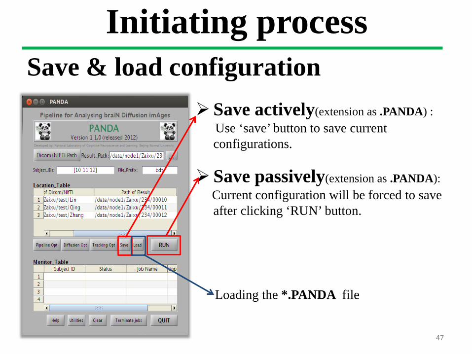
Initiating processSave & load configuration

Save actively(extension as .PANDA) :Use ‘save’ button to save current configurations.

Save passively(extension as .PANDA):Current configuration will be forced to save after clicking ‘RUN’ button.

Loading the *.PANDA file

47


48

Contents

Monitoring progress

Subject ID(fixed)

You can load the *.PANDA file to re-monitor the progress anytime, after shutting down PANDA or even Matlab

Status(dynamic)waitsubmittedrunningfinishedfailed

Job Name(dynamic)

Unprocessed Step(dynamic)

49

Monitoring progress

50

Terminate jobs

Terminate all the jobs runningin background.


51

Contents

Understanding resultant files

52

DICOM Path Result Path

Understanding resultant files Folder native_space:

53

Understanding resultant files Native space In the folder named ‘native_space’

Origin FA (Fractional Anisotropy):*_FA.nii.gz

Origin MD (Mean Diffusivity):*_MD.nii.gz

1st eigenvalue (Axial Diffusivity):*_L1.nii.gz

2nd eigenvalue:*_L2.nii.gz

3rd eigenvalue:*_L3.nii.gz

Radial Diffusivity:*_L23m.nii.gz

b0:*_S0.nii.gz, data_b0_eddy.nii.gz

1st eigenvector:*_V1.nii.gz

2nd eigenvector:*_V2.nii.gz

3rd eigenvector:*_V3.nii.gz

54

Understanding resultant files Native space In the folder named ‘native_space’

b value file:bvals

b vector file:bvecs

brain mask:nodif_brain_mask

4D image data:data.nii.gz

T1 normalization to MNI152 space:*_2MNI152.nii.gz

FA normalization to T1 image:*_T1.nii.gz

parcellated image (native space):*_Parcellated_*

55

Understanding resultant files Folder quality_control:

56

Understanding resultant files Check Quantity In the folder named ‘quantity_control’

Check quantity of FA:FA -> *_FA_QC.png

Check quantity of FA normalization to Template:FA_Normalized_1mm -> slicesdir -> *

Check quantity of FA normalization to T1:FA_Normalized_1mm -> slicesdir -> *

Check quantity of T1:T1 -> *_QC.png

Check quantity of T1:T1 -> *_QC.png

Check quantity of T1 normalization to MNI152 space:T1_to_MNI152 -> slicesdir -> * 57

Understanding resultant files Folder standard_space:

58

Understanding resultant files

• Resultant images in MNI space with 1mm×1mm×1mm resolution *_FA_4normalize_to_target_1mm.nii.gz : FA image*_MD_4normalize_to_target_1mm.nii.gz : MD image*_L1_4normalize_to_target_1mm.nii.gz : image*_L23m_4normalize_to_target_1mm.nii.gz : image

• Resultant images in MNI space with 2mm×2mm×2mm resolution*_FA_4normalize_to_target_2mm.nii.gz :FA image in 2×2×2 standard space*_MD_4normalize_to_target_2mm.nii.gz :MD image in 2×2×2 standard space*_L1_4normalize_to_target_2mm.nii.gz : image in 2×2×2 standard space*_L23m_4normalize_to_target_2mm.nii.gz : image in 2×2×2 standard space

• Resultant images after Gaussian smoothing *_FA_4normalize_to_target_2mm_s6mm.nii.gz : smoothing images of 2×2×2 FA image *_MD_4normalize_to_target_2mm_s6mm.nii.gz : smoothing images of 2×2×2 MD image *_L1_4normalize_to_target_2mm_s6mm.nii.gz : smoothing images of 2×2×2 image *_L23m_4normalize_to_target_2mm_s6mm.nii.gz :

smoothing images of 2×2×2 image (s6mm means that smoothing kernel size is 6mm)

Voxel-level results In the folder named ‘standard_space’

1λ

23mλ

1λ23mλ

1λ

23mλ

59

Understanding resultant files Regional-level results

• Regional results based on atlas*_FA_4normalize_to_target_1mm.WMlabel :

regional FA average based on WMlabel-atlas*_FA_4normalize_to_target_1mm.WMtract :

regional FA average based on WMtract-atlas*_MD_4normalize_to_target_1mm.WMlabel :

regional MD average based on WMlabel-atlas*_MD_4normalize_to_target_1mm.WMtract :

regional MD average based on WMtract-atlas*_L1_4normalize_to_target_1mm.WMlabel :

regional average based on WMlabel-atlas*_L1_4normalize_to_target_1mm.WMtract :

regional average based on WMtract-atlas*_L23m_4normalize_to_target_1mm.WMlabel :

regional average based on WMlabel-atlas*_L23m_4normalize_to_target_1mm.WMtract :

regional average based on WMtract-atlas

In the folder named ‘standard_space’

1λ

1λ

23mλ

23mλ60

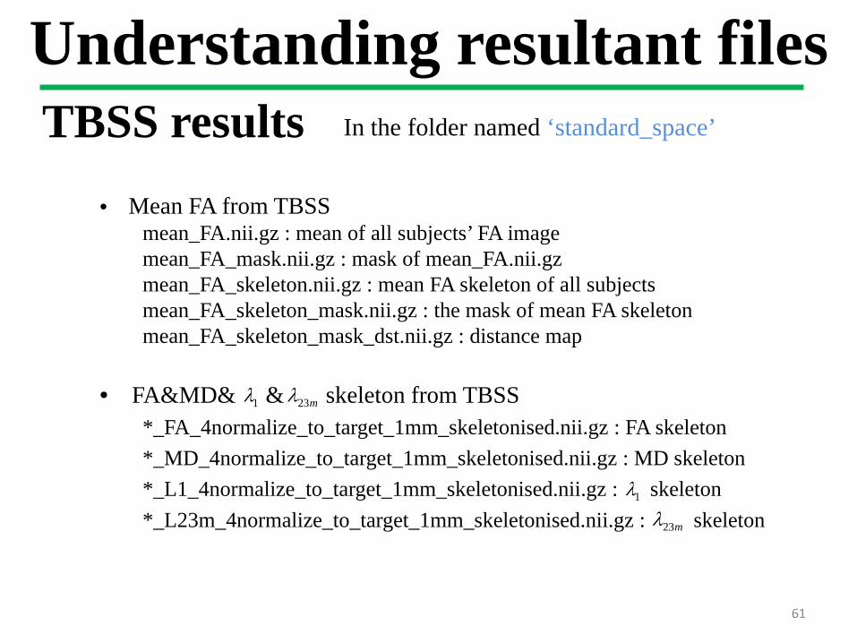
Understanding resultant files TBSS results

• FA&MD& & skeleton from TBSS*_FA_4normalize_to_target_1mm_skeletonised.nii.gz : FA skeleton*_MD_4normalize_to_target_1mm_skeletonised.nii.gz : MD skeleton*_L1_4normalize_to_target_1mm_skeletonised.nii.gz : skeleton*_L23m_4normalize_to_target_1mm_skeletonised.nii.gz : skeleton

• Mean FA from TBSSmean_FA.nii.gz : mean of all subjects’ FA image mean_FA_mask.nii.gz : mask of mean_FA.nii.gzmean_FA_skeleton.nii.gz : mean FA skeleton of all subjectsmean_FA_skeleton_mask.nii.gz : the mask of mean FA skeleton mean_FA_skeleton_mask_dst.nii.gz : distance map

In the folder named ‘standard_space’

23mλ1λ

1λ 23mλ

61

Understanding resultant files Folder trackvis:

62

Understanding resultant files Deterministic Fiber Tracking In the folder named ‘trackvis’

track file :dti_*.trk

track file after applying spline filter:dti_*_S.trk

You can open .trk file with Trackvis Software (http://www.trackvis.org/) to draw ROI and do statistical analysis.

63

Understanding resultant files Deterministic Fiber Tracking In the folder named ‘trackvis’ FA:

dti_fa.nii.gz

color FA:dti_fa_color.nii.gz

MD:dti_adc.nii.gz

b0:dti_b0.nii.gz

1st eigenvector:dti_v1.nii.gz

2nd eigenvector:dti_v2.nii.gz

3rd eigenvector:dti_v3.nii.gz

1st eigenvalue:dti_e1.nii.gz

2nd eigenvalue:dti_e2.nii.gz

3rd eigenvalue:dti_e3.nii.gz

4D data:dti_dwi.nii.gz

b vector file:ForDTK_bvecs 64

Understanding resultant files Folder Network:

65

Understanding resultant files Deterministic Network In the folder named ‘Network/Deterministic’

*_Matrix_FA_*: average FA of all the voxels along the fibers between two regions

*_Matrix_FN_*: fiber number between two regions

*_Matrix_Length_*: average length of fibers between two regions

66

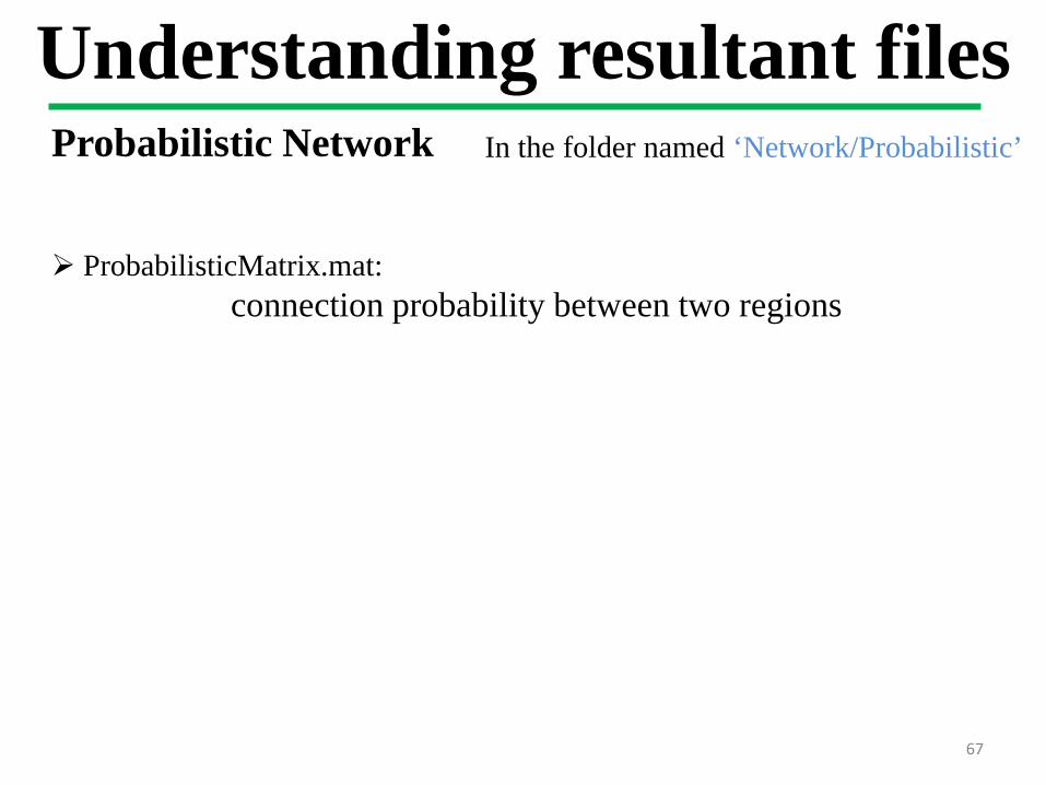
Understanding resultant files Probabilistic Network In the folder named ‘Network/Probabilistic’

ProbabilisticMatrix.mat:connection probability between two regions

67


68

Contents

69

Utilities

70

Utilities (TBSS)Run TBSS for a group of subjects in parallel

71

Utilities (TBSS)FA Path:

full path of subjects’ 1*1*1 FA image

Data Path:full path of 1*1*1 data to

be projected to the average skeleton, such as

FA, MD, ,

Threshold:FA threshold to exclude voxels in the grey matter

or CSF

Result Path:full path of TBSS results

‘Data Path’ button can be clicked several times. Click ‘Data Path’ button once, user can add one type of data. The order of the Data path must be in accordance with FA path.

1λ 23mλ

72

Utilities (TBSS)

Referring to: Pipeline_Opt

Referring to: Monitoring Progress

Current configuration will be forced to save after

clicking ‘RUN’ button.(extension as .PANDA_TBSS)

Loading the *.PANDA _TBSS file

73

Utilities (TBSS)Set FA Path:

74

Utilities (TBSS)Set Data1 Path:

75

Utilities (TBSS)Set Data2 Path:

76

Utilities (TBSS)Set Result Path:

77

Utilities (TBSS)Initiating Process:

78

Utilities (TBSS)Resultant Files:

First: mean FA and mean FA skeleton will be produced in ‘TBSS’ folder .

Next: map mean FA skeleton to native data (FA, MD, , .etc), resulting in native skeleton.

Native MD skeleton

Mean FA & Mean FA skeleton

1λ 23mλ

79

Utilities (Brain Parcellation)Run brain parcellation according to atlas for any

number of subjects in parallel

80

Utilities (Brain Parcellation)

Atlas (standard space):full path of atlas in the standard space, such as

AAL atlas

T1 Path:full path of subjects’ T1

images

The order of T1 path must be in accordance with the order of FA path

FA Path:full path of subjects’ FA

images

81

Utilities (Brain Parcellation)



Current configuration will be forced to save after clicking ‘RUN’ button. (extension as

.PANDA_BrainParcellation)

Loading the *.PANDA _BrainParcellation file

Utilities (Brain Parcellation)Set FA Path:

82

Utilities (Brain Parcellation)Set T1 Path:

83

84

Utilities (Brain Parcellation)Initiating Process:

Utilities (Brain Parcellation)Resultant Files:

Parcellated image for subject 00010

A file named ‘*_Parcellated_*.nii.gz ’ will be produced in the same folder of FA.

In this example:Path of FA images are

/data/node1/Zaixu/234/00010/native/bd_00010_FA.nii.gz

/data/node1/Zaixu/234/00011/native/bd_00011_FA.nii.gz

/data/node1/Zaixu/234/00012/native/bd_00012_FA.nii.gzOutputs are

/data/node1/Zaixu/234/00010/native/bd_00010_FA_Parcellated_*.nii.gz

/data/node1/Zaixu/234/00011/native/bd_00011_FA_Parcellated_*.nii.gz

/data/node1/Zaixu/234/00012/native/bd_00012_FA_Parcellated_*.nii.gz 85

86

Utilities (BedpostX) Run bedpostX for any number of subjects in parallel

87

Utilities (BedpostX)Subject Folders List:full path of subjects’ folders which contain

mask, bvecs, bvals and 4D data

Fibers:Number of fibers per

voxel, default 2

Weight:ARD weight, more weight

means less secondary fibers per voxel, default 1

Burnin:Burnin period, default

1000

88

Utilities (BedpostX)




clicking ‘RUN’ button.(extension as .PANDA_BedpostX)

Loading the *.PANDA _BedpostX file

89

Utilities (BedpostX)Input subjects’ folder:

90

Utilities (BedpostX)Initiating Process:

91

Utilities (BedpostX)Resultant Files:

Bedpostx result for subject 00010



A folder named ‘*.bedpostX’ will be produced for each subject.

In this example:Inputs are

/data/node1/Zaixu/234/00010/native/data/node1/Zaixu/234/00011/native/data/node1/Zaixu/234/00012/native

Outputs are/data/node1/Zaixu/234/00010/native.bedpostX/data/node1/Zaixu/234/00011/native.bedpostX/data/node1/Zaixu/234/00012/native.bedpostX

92

Utilities (Tracking & Network) Run Tracking & Network Construction for any number of

subjects in parallel

93

Utilities (Tracking & Network)With PANDA_Tracking GUI, you can do:

Deterministic Fiber Tracking

Deterministic Network Construction

Probabilistic Fiber Tracking & Network Construction

BedpostX & Probabilistic Fiber Tracking & Network Construction

94

Utilities (Tracking & Network)Deterministic Fiber Tracking

Second step: select Deterministic Fiber Tracking Referring to: Deterministic Fiber Tracking

First step: input subjects’ folders which contain

bvces, bvals, mask and 4D data

95

Utilities (Tracking & Network)

Second step: select Network Node Definition Referring to: Next Page

Deterministic Network ConstructionFirst step: select Deterministic Fiber Tracking

Referring to: Deterministic Fiber Tracking

Third step: select Deterministic Network Construction

96

Utilities (Tracking & Network)Network Node DefinitionFirst, please click ‘FA Path’ button to input subjects’ FA paths

The order of paths of parcellated images or T1 images must be in accordance with the order of the paths of FA images .

When you have parcellated images in native space :Please select ‘Parcellated (native space) ’ and input these images

When you don’t have parcellatedimages in native space :Please select ‘T1 images’ and input these images

97

Utilities (Tracking & Network)Probabilistic Fiber Tracking & Network Construction

Third step: select Probabilistic Network ConstructionReferring to Next Page

Second step: select Network Node Definition, Referring to: Network Node Definition

First step: input subjects’ bedpostXresult folder

98

Utilities (Tracking & Network)Probabilistic Fiber Tracking & Network Construction

Tracking Type:OPD(output path distribution);

PD(Correct path distribution for the length of the pathways and

output path distribution)

Label ID:the id of brain region in atlas

99

Utilities (Tracking & Network)BedpoxtX+Probabilistic Fiber Tracking & Network Construction

Third step: select Bedpostx+ProbabilisticNetwork ConstructionReferring to Next Page

Second step: select Network Node Definition, Referring to: Network Node Definition

First step: input subjects’ folder which contain bvces, bvals, mask, 4D data

100


Referring to: Network Node Definition

BedpoxtX+Probabilistic Fiber Tracking & Network Construction

101




clicking ‘RUN’ button.(extension as .PANDA_Tracking)

Loading the *.PANDA _Tracking file


102

Utilities (Tracking & Network)Resultant Files (Deterministic Fiber Tracking):

Deterministic fiber tracking result for subject 00010



A folder named ‘trackvis’ will be produced for each subject.



Outputs are/data/node1/Zaixu/234/00010/trackvis/data/node1/Zaixu/234/00011/trackvis/data/node1/Zaixu/234/00012/trackvis

103

Utilities (Tracking & Network)Resultant Files(Deterministic Network Construction):

A folder named ‘Network’ will be produced for each subject, then a folder named ‘Deterministic’ will be produced in the folder ‘Network’.



Outputs are/data/node1/Zaixu/234/00010/Network/Deterministic/data/node1/Zaixu/234/00011/Network/Deterministic/data/node1/Zaixu/234/00012/Network/Deterministic

104


104

Resultant Files (Probabilistic Network Construction):A folder named ‘Network’ will be produced for each subject, then a folder named ‘Probabilistic’ will be produced in the folder ‘Network’.



Outputs are/data/node1/Zaixu/234/00010/Network/Probabilistic/data/node1/Zaixu/234/00011/Network/Probabilistic/data/node1/Zaixu/234/00012/Network/Probabilistic

105

Utilities (DICOM Sorter) Sort DICOM files into different series

106

Utilities (DICOM Sorter)DICOM Path:

the full path of subjects’ folders which contain all the DICOM files to be

sorted

DICOM File Suffix:The extension of DICOM

file name

If you input the DICOM file suffix, it will sort all the files with the extension as the suffix under subjects’ DICOM folders.If the DICOM_File_Suffix is empty, it will sort all the files under subjects’ DICOM folders.

Utilities (DICOM Sorter)

107

108

Utilities (Image Converter) Convert image format among (.nii, .nii.gz, .img)

109

Utilities (Image Converter)

Image Files Path:the full path of image files

(.nii, .nii.gz, .img) to be converted

Result Format:3 choices (NIFTI,

NIFTI_GZ, NIFTI_PAIR)

After the conversion, new image files will replace the origin image files.

110

Utilities (Image Converter)

111

Utilities (File Copyer) Copy files to the destination path

112

Utilities (File Copyer)

Source Files Path:full path of files users

want to copy

Destination Path:the path user wants to

save these files

113


114


Acknowledgement

FSL (see page 6)http://www.fmrib.ox.ac.uk/fsl/

PSOM (manage pipelines, see page 7)http://code.google.com/p/psom/

Diffusion Toolkit (see page 6)http://www.trackvis.org/dtk/

MRICRON (see page 6)http://www.mccauslandcenter.sc.edu/mricro/mricron

115

Help

Please report bugs or requests to:

Zaixu Cui: [email protected]

Suyu Zhong: [email protected]

Gaolang Gong (PI): [email protected]

116

mailto:[email protected]�



panda manual

Documents