panel unit root and cointegration methods
TRANSCRIPT

Panel unit root and cointegration methods
Mauro Costantini
University of Vienna, Dept. of Economics
Master in Economics
Vienna
2010
Mauro Costantini Panel unit root and cointegration methods

Outline of the talk (1)
Unit root, cointegration and estimation in time
series.
1a) Unit Root tests (Dickey-Fuller Test, 1979);
2a) Cointegration tests: single equation method
(Engle-Granger, 1987);
3a) Estimators: OLS, DOLS (Saikkonen, 1991), FMOLS
(Phillips and Hansen, 1990).
Mauro Costantini Panel unit root and cointegration methods

Outline of the talk (2)
Unit root, cointegration and estimation in panel
data.
1b) Limits of time series approach;
2b) Advantages and Disadvantages of the nonstationary panel
methods.
3b) First and second generation of panel unit root tests,
cointegration and estimation methods.
Mauro Costantini Panel unit root and cointegration methods

Time series unit root tests: regression equation (1)
yt = ρyt−1 + εt (1)
∆yt = βyt−1 + εt (2)
where β = (ρ− 1) and εt is white noise process
(E(ε) = 0,E(ε2t ) = σ2 < ∞,E(etej) = 0, for t 6= j). The test of
H0 : β = 0 (ρ = 1) has a non-standard distribution (Brownian or
Wiener process).
Mauro Costantini Panel unit root and cointegration methods

Asymptotic distribution of Dickey-Fuller tests (2)
Given t observation, the OLS estimator of ρ in (1) is:
ρ =
( T∑
t=1
y2t−1
)−1 T∑
t=1
ytyt−1 (3)
The limiting distribution of the OLS estimator ρ when ρ = 1 is:
T (ρ− 1) ⇒∫ 10 W (r)dW (r)∫ 1
0 W (r)2dr=
(1/2)[W (1)]2 − 1∫ 10 [W (R)]2dr
(4)
The previous distribution can be used for testing the unit root null
hypothesis H0 : ρ = 1, that’s K = T(ρ− 1) or we can normalize it
with the standard of the OLS estimator and construct the
t-statistics.
Mauro Costantini Panel unit root and cointegration methods

Asymptotic distribution of Dickey-Fuller tests (3)
The test statistics is:
tρ =(ρ− 1)
σρ=
(ρ− 1)
s2 ÷∑Tt=1 y2
t−11/2, (5)
where σρ is the usual OLS standard error for the estimated
coefficient and s2 denotes the OLS estimate of the residual
variance:
s2 =
∑Tt=1(yt − ρyt−1)
2
T − 1(6)
as T →∞,
tρ →∫ 10 W (r)dW (r)
[∫ 10 W (r)2dr ]1/2
=1/2[W (1)2 − 1][∫ 1
0 W (r)2dr ]1/2, (7)
Mauro Costantini Panel unit root and cointegration methods

Cointegration: concept (1)
An important property of I(1) variables is that a linear combination
of these two variables that is I(0) may exist. If this is the case,
these variables are said to be cointegrated. The concept of
cointegration was introduced by Granger (1981). Consider two
variables yt and xt that are I(1). Then yt and xt are said to be
cointegrated if there exist a β such that yt − βxt is I(0). We
denoted this as CI (1, 1). More generally, if yt is I(d) and and xt is
I(d), then yt and xt are CI (d , b) if yt − βxt is I (d − b) with b > 0.
Mauro Costantini Panel unit root and cointegration methods

Cointegration: concept (2)
What the previous concept means is that the regression equation:
yt = βxt + µt (8)
makes sense since yt and xt do not drift too far apart each other
over time. Thus, there is a long run equilibrium relationship
between them (see the geometric interpretation of cointegration
below). If yt and xt are not cointegrated, that is yt − βxt = µt is
also I(1), then yt and xt would drift apart from each other over
time. In this case, the relationship between yt and xt that we
obtain by regressing yt on xt would be spurious.
Mauro Costantini Panel unit root and cointegration methods

Cointegration: graphics (1)
Nominal interest rate on a 20 year US saving and loan credit instrument (R20) and AAA Moodys bond rate (R30)
Mauro Costantini Panel unit root and cointegration methods

Cointegration: geometric interpretation (4)
Suppose pit > pjt , demand will go to location j : i.) Shocks to the
economy make us to move out of the equilibrium; ii.) The
adjustment does not have to be instantaneous but eventually; iii.)
Long run equilibrium pit = pjt , this us a linear attractor
45°
1 1 1( )i jp p 2
1 1( )i jp p
3
3 3( )i jp p
4
5
it jtp pjtp
itp
Mauro Costantini Panel unit root and cointegration methods

Cointegration Tests: Engel and Granger model (1)
Consider two series y1t ∼ I(1), y2t ∼ I(1) and a simple
two-equation model:
y1t = βy2t + u1t , u1t = u1t−1 + ε1t , (9)
y1t = αy2t + u2t , u2t = ρu2t−1 + ε2t , |ρ| < 1 (10)
The second equation describes a particular combination of the
series which is stationary. Hence y1t and y2t are C(1,1). The null
hypothesis is taken to be no co-integration or ρ = 1 in (10).
Mauro Costantini Panel unit root and cointegration methods

Cointegration Tests: Engel and Granger model (2)
1. The cointegrating equation (10) is estimated by OLS and the
residuals are saved.
2. Several tests on the residual are provided (i.e. Durbin-Watson,
Dickey-Fuller and Augmented Dickey-Fuller). If the residuals
are nonstationary, the series are no cointegrated. Otherwise,
the series are cointegrated.
For examples, if the residuals are nonstationary, the DW test will
approach to zero and thus the test rejects no co-integration
hypothesis if DW is too big.
Mauro Costantini Panel unit root and cointegration methods

Cointegration Tests: Engel and Granger model (3)
Consider again y1t and y2t that are both I(1). Suppose there is
cointegration, that’s ut in (10) is I(0) and α is the cointegrating
vector (for the case of two variables, scalar). If there is
cointegration, we can show that α is unique. Because, if we have
y1t = γy2t + v2t where v2t is also I(0), by substraction we have
(α− γ)y2t + u2t − v2t is I(0). But u2t − v2t is I(0) which means
(α− γ)y2t is I(0). This is not possible since y2t is I(1).
Mauro Costantini Panel unit root and cointegration methods

Cointegration Tests: Engel and Granger model (4)
The equation-system (9-10), can be re-written in reduced as
follows:
y1t =α
α− βu1t − β
α− βu2t (11)
y2t =1
α− βu1t − 1
α− βu2t (12)
These equation show that both y1t and y2t are driven by a
common I(1) variable. This is known as the common trend
representation of the cointegrated system.
Mauro Costantini Panel unit root and cointegration methods

OLS estimator (1)
If the variables in (10) are not cointegrated, ρ = 1, then the OLS
is quite likely to produce spurious results (high R2, t-statistics that
appear to be significant), but the results are without economic
results (if the residuals have a stochastic trend, any error in period
t never decays, so that the deviation from the model is permanent.
It’s hard to imagine attaching any importance to an economic
model having permanent errors).
Mauro Costantini Panel unit root and cointegration methods

OLS estimator (2)
Stock (1987) show that OLS estimator is superconsistent: α
converge to its true value at the rate T(superconsistency) instead
of the usual rate√
T (consistency). Although α is superconsistent,
Banerjee et al. (1986) and Banerjee et al. (1993) show that
through Monte Carlo studies that there can be substantial sample
biases (the dynamic is missed). This missing information also
causes the DF test in the Engle-Granger approach to be less
powerful than the cointegration test based on the t-statistics in the
Error Correction model (ECM)
Mauro Costantini Panel unit root and cointegration methods

OLS estimator and the dynamic model (ECM)(1)
Consider the following ADL(1,1) model:
yt = α0 + α1yt−1 + β0zt + β1zt−1 + εt (13)
where εt ∼ iid(0, σ2) and |α1| < 1. In a statistic equilibrium (all
changes has ceased), we have E (yt) = E (yt−1) = ... = y∗ and
E (zt) = E (zt−1) = ... = z∗.
Mauro Costantini Panel unit root and cointegration methods

OLS estimator and the dynamic model (ECM)(2)
By getting the expectation of (13), we have:
y∗ = α0 + α1y∗ + β0zt + β1z
∗ (14)
and then
y∗ =α0 + (β0 + β1)z
∗
1− α1≡ k0 + k1z
∗ (15)
or
E (yt) = k0 + k1E (zt) (16)
where k1 is the long-run multiplier of y with respect to z.
Mauro Costantini Panel unit root and cointegration methods

OLS estimator and the dynamic model (ECM)(3)
Now subtract yt−1 from both side of (13) and then add and
subtract β0zt−1 on the right-hand side to get:
∆yt = α0 + (α1 − 1)yt−1 + β0∆zt + (β0 + β1)zt−1 + εt (17)
and finally add and subtract (α1− 1)zt−1 on the right side, yielding
∆yt = α0+(α1−1)(yt−1−zt−1)+β0∆zt+(β0+β1+α1−1)zt−1+εt
(18)
Mauro Costantini Panel unit root and cointegration methods

OLS estimator and the dynamic model (ECM)(4)
Alternatively, we could have added and subtracted (β0 + β1)zt−1
on the right side, to get
∆yt = α0 + (α1 − 1)(yt−1 − k1zt−1) + β0∆zt + εt (19)
where (α1 − 1) represents the short-run adjustment to a
’discrepancy’ (a measure of the speed of adjustment of y to a
discrepancy between y and z in the previous period).
Mauro Costantini Panel unit root and cointegration methods

Dynamic model and cointegration test (1)
Write in a different form (19) with no constant term:
∆yt = a∆zt + b(y − z)t−1 + εt (20)
The parameter b is the error correction coefficient. For yt = lnY
and z = lnZ , a denotes the short run-elasticity of Y with respect
to Z. Without loss of generality, the cointegrating vector for
(yt , zt)′is (1,-1) if yt and zt are cointegrated. We assume, for
simplicity, that the cointegrating vector is known.
Mauro Costantini Panel unit root and cointegration methods

Dynamic model and cointegration test (2)
The variable yt and zt are cointegrated, or not, depending on
whether b < 0 and b = 0. Thus, tests of cointegration rely on
upon some estimate of b. In ECM approach, equation (20) is
estimated by OLS
∆yt = a∆zt + bwt−1 + εt (21)
where the disequilibrium is:
wt = yt − zt (22)
The t-statistics based on b is the ECM statistics, tECM . It is used
to test the null hypothesis that b = 0, i.e, that yt and zt are not
cointegrated with cointegrating vector [1,-1].Mauro Costantini Panel unit root and cointegration methods

Dynamic model and cointegration test (3)
The DF statistics derives form a different regression, so it’s helpful
to establish the relationship between the DF regression equation
and the ECM in (20). Subtract ∆zt from both side of (20) and
re-arrange:
∆(y − z)t = b(y − z)t + [(a− 1)∆zt + εt ] (23)
Mauro Costantini Panel unit root and cointegration methods

Dynamic model and cointegration test (4)
It should be noted that (22) and (23) can be rewritten as:
∆wt = bwt + et (24)
where the disturbance et is
et = (a− 1)∆zt + εt ] (25)
Mauro Costantini Panel unit root and cointegration methods

Dynamic model and cointegration test (5)
OLS estimation of (24) generates:
∆wt = bwt + et (26)
The t-statistics based on b is the DF statistics, TDF . This statistics
is also used for testing whether yt and zt are cointegrated.
Mauro Costantini Panel unit root and cointegration methods

Dynamic model and cointegration test (6)
In contrast to the estimated ECM in (21), the estimated DF
equation (26) ignores potential information contained in ∆zt
Mauro Costantini Panel unit root and cointegration methods

OLS estimator, endogeneity and serial correlation
In addition, the asymptotic distribution of the OLS estimator
depends on nuisance parameters arising from endogenity of the
regressors and serial correlation in the errors. To solve these
problems, two estimators are proposed: FMOLS (fully modified
OLS) and DOLS (dynamic OLS)
Mauro Costantini Panel unit root and cointegration methods

FMOLS estimator (1)
Consider the following model:
yt = µ + β′xt + u1t = θ
′zt + u1t , (27)
∆xt = u2t , (28)
for t = 1, ..., T , θ = (µ, β′)′, zt = (1, x
′t)′. For ut = [u1t , u2t ], we
assume that the functional central limit theorem (FCLT) can be
applied as follows:
1√T
[Tr ]∑
t=1
⇒ W (r) =
W1(r)
W2(r)
(29)
for 0 ≤ r ≤ 1, where W (r) is a Brownian motion on [0, 1] with a
variance-covariance matrix Ω (W (·) ∼ BM(Ω)).Mauro Costantini Panel unit root and cointegration methods

FMOLS estimator (2)
Note that the long-run variance of ut and its one-sided version can
be expressed as Ω = Σu + Π + Π′
Λ = Σu + Π, with Σu = limT→∞
T−1∑T
t=1 E (utu′t) and
Π = limT→∞
T−1∑T−1
j=1
∑T−jt=1 E (utu
′t+j).
Mauro Costantini Panel unit root and cointegration methods

FMOLS estimator (3)
Ω and Λ can be conformably partioned with ut as:
Ω =
ω11 ω12
ω21 Ω22
Λ =
λ11 λ12
λ21 Λ22
Mauro Costantini Panel unit root and cointegration methods

FMOLS estimator (4)
It is known that the OLS estimator of θ, denoted by θ, is consistent
but inefficient in general. The centered OLS estimator with a
normalizing matrix DT = diag√
T , TIn weakly converges to
DT (θ − θ) ⇒( ∫ 1
0W2(r)W
′2(r)dr
)−1(∫ 1
0W2(r)dW1(r) + λ21
)
(30)
and we can observe that this limiting distribution contains the
second-order bias from the correlation between W1(·) and W2(·)and the non-centrality parameter λ21.
Mauro Costantini Panel unit root and cointegration methods

FMOLS estimator (5)
As explained in Phillips and Hansen (1990) and Phillips (1995),
the former bias arises from the endogeneity of the I(1) regressor xt
while the non-centrality bias comes from the fact that the
regression errors are serially correlated. Phillips and Hansen (1990)
argue that the second-order biases have no effect on the
consistency of the estimators, but result in asymptotic distributions
of scaled estimators, such as T (β − β) in (27), having non-zero
means.
Mauro Costantini Panel unit root and cointegration methods

FMOLS estimator (6)
In order to eliminate the second-order bias, Phillips and Hansen
(1990) proposes correcting the single-equation estimates
non-parametrically in order to obtain meadian-unbiased and
asymptotically normal estimates.
Mauro Costantini Panel unit root and cointegration methods

FMOLS estimator (6)
The Fully modified OLS is:
θ+ =
( T∑
t=1
ztz′t
)−1( T∑
t=1
zty+t − TJ+
)(31)
where the transformations:
y+t = yt − ω12Ω
−122 u2t (32)
and
J+ =
0
λ2 − Λ22ˆΩ−122 ω21
(33)
allows for correcting for the endogeneity bias and the
non-centrality bias.Mauro Costantini Panel unit root and cointegration methods

DOLS Estimator (1)
Contrary to nonparametric approach provided by Phillips and
Hansen, the DOLS method proposed by Saikkonen (1991) is based
on parametric regressions. Saikkonen proposes to augment the
leads and lags of the first difference of y2t as regressors and to
estimate
yt = θ′zt +
K∑
j=−K
π′j∆xt−j + u1t , (34)
Mauro Costantini Panel unit root and cointegration methods

DOLS Estimator (2)
The DOLS estimator is defined as the OLS of θ for (84)
θ′=
( T−K∑
t=K+1
zt z′t
)−1( T−K∑
t=K+1
zt y1t
)(35)
where zt and y1t are regression residuals of zt and yt on
wt = (u′2,t+K , ........, u
′2,t−K ), respectively.
Mauro Costantini Panel unit root and cointegration methods
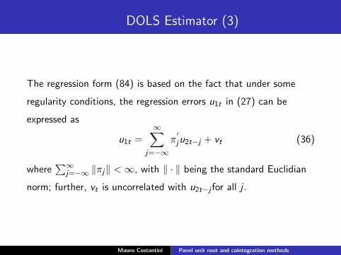
DOLS Estimator (3)
The regression form (84) is based on the fact that under some
regularity conditions, the regression errors u1t in (27) can be
expressed as
u1t =∞∑
j=−∞π′ju2t−j + vt (36)
where∑∞
j=−∞ ‖πj‖ < ∞, with ‖ · ‖ being the standard Euclidian
norm; further, vt is uncorrelated with u2t−j for all j .
Mauro Costantini Panel unit root and cointegration methods

DOLS Estimator (4)
From (36), we observe that
u1t =∑
|j |>K
π′ju2t−j + vt (37)
The uncorrelatedness of vt with all the leads and lags of u2t is an
important property to prove that the DOLS method successfully
eliminates the second-order bias of the OLS Estimator.
Mauro Costantini Panel unit root and cointegration methods

Some limits of time series approach
1. In time series analysis with unit root processes, many of the
estimators and statistics of interest have been shown to have
limiting distributions which are complicated functionals of
Wiener processes.
2. The power deficiencies of pure time series-based tests for unit
roots and cointegration .
Mauro Costantini Panel unit root and cointegration methods
Low power of unit root tests (1)
Finite sample properties
Monte Carlo simulations have shown that the power of the various
Dickey-Fuller and Phillips-Perron tests is very low; unit root tests
do not have power to distinguish between a unit root and near unit
root process (see Dickey and Fuller, 1997). Thus, these test will
too often indicate that a series contains a unit root. Moreover,
they have a little power to distinguish between trend stationary
and drifting processes. In finite sample, any trend stationary
process can be arbitrarily well approximated by a unit root process,
and a unit root process ca be arbitrarily well approximated by a
trend stationary process.
Mauro Costantini Panel unit root and cointegration methods

Low power of unit root tests (2)
Finite sample properties
Consider the following random walk plus noise model:
yt = µt + ηt (38)
µt = µt−1 + εt (39)
where ηt and εt are both independent white-noise process with
variance of σ2η and σ2, respectively. Suppose that we can observe
the yt sequence, but cannot directly observe the separate shocks
affecting yt.
Mauro Costantini Panel unit root and cointegration methods

Low power of unit root tests (3)
Finite sample properties
If σ2 6= 0, yt is the unit root process:
yt = µ0 +T∑
t=1
εt + ηt (40)
If σ2 = 0, then all values of εt are constant, that’s:
εt = εt1 = ... = ε0. Now, define this initial values of ε0 as a0. It
follows that
µt = µ0 + a0t
and yt is trend stationary:
yt = µ0 + a0t + ηt (41)
Mauro Costantini Panel unit root and cointegration methods

Low power of unit root tests (4)
Finite sample properties
The difference between the difference stationary process (40) and
trend process (41) concerns the variance of εt. Since we observe
the composite effect of the two shocks, but not the individual
components ηt and εt, we can see that there is no simple way to
determine whether σ2 is exactly equal to zero, in particular when
the Data Generating Process (DGP) is such that σ2η is large
relative to σ2. In a finite sample, arbitrarily increase σ2η will make
it virtually impossible to distinguish a TS and DS series.
Mauro Costantini Panel unit root and cointegration methods

Low power of unit root tests (5)
Finite sample properties
In addition, it also follows that a trend stationary process can be
arbitrarily well approximate a unit root process. If the stochastic
portion of the the trend stationary process has sufficient variance,
it will be not possible to distinguish between the unit root and the
trend stationary hypothesis.
Mauro Costantini Panel unit root and cointegration methods

Low power of unit root tests (6)
For example, the random walk plus drift model:
yt = a0 + yt−1 + εt ,
can be arbitrarily well represented by the model
yt = a0 + ρyt−1 + εt
by increasing σ2 and allowing ρ to be close to unity. Both these
models can be approximated by (41).
Mauro Costantini Panel unit root and cointegration methods

Low power of unit root tests (7)
For applications
It turns out that for tests of unit root hypothesis versus stationary
alternatives the power depends very little on the number of
observations per se but is rather influenced in an important way by
the span of the data. For a given number of observations, the
power is largest when the span is longest. For a given span,
additional observation obtained using data sampled more
frequently lead only to a marginal increase in power, the increase
becoming negligible as the sampling interval is decreased (Perron,
1990, JBES).
Mauro Costantini Panel unit root and cointegration methods

Low power of unit root tests (8)
In most applications os interest, a data set containing fewer annual
data over a long time period will lead to tests having higher power
than if use was made of a data set containing more observations
over a short time period. These results show that, whenever
possible, tests of unit root hypothesis should be performed using
annual data over a long time period.
Mauro Costantini Panel unit root and cointegration methods

Nonstationary Panel data
With the growing use of cross-country data over time to study
purchasing power parity, growth convergence and international
R&D spillovers, the focus of panel data econometrics has shifted
towards studying the asymptotics of macro panels with large
N(number of countries) and large T (length of the time series)
rather than the usual asymptotics of micro panels with large N and
small T. A strand of literature applied time series procedures to
panels, worrying about nonstationarity, spurious regression and
cointegration.
Mauro Costantini Panel unit root and cointegration methods

Why nonstationary panel data? Advantages...
1. The use of data from countries for which the span of time
series data is insufficient and would in this way preclude the
analysis of many economic hypothesis of interest;
2. The benefits coming from better power properties of the
testing procedure with respect to standard time series
technique;
3. The fact that many issue of economic interest, such as
convergence or purchasing power parity lend themselves
naturally to being analyzed in a panel framework;
4. Unit root and cointegration tests have Normal standard
asymptotic distribution.
Mauro Costantini Panel unit root and cointegration methods

...Disavantages (1)
1. Panel data generally introduce a substantial amount of
unobserved heterogeneity, rendering the parameters of the model
cross section specific;
2. The panel test outcomes are often difficult to interpret if the
null of the unit root or cointegration is rejected. The best that can
be concluded is that ”a significant fraction of the cross section
units is stationary or cointegrated”. The panel tests do not provide
explicit guidance as to the size of this fraction or the identity of
the cross section units that are stationary or cointegrated;
Mauro Costantini Panel unit root and cointegration methods

...Disavantages (2)
3. With unobserved I(1) common factors affecting some or all the
variables in the panel, it is also necessary to consider the possibility
of cointegration between the variables across the groups (cross
section cointegration) as well as within group cointegration;
Mauro Costantini Panel unit root and cointegration methods

...Disavantages (3)
4. Economic applications. For example, panel unit root tests are
not able to rescue purchasing power parity (PPP). The results on
PPP with panels are mixed depending ont the group of countries
studied, the period of study and the type of unit root test used. In
addition, for PPP, series. The null hypothesis of a single time
series is different from the null hypothesis of panel data, so the
panel data tests are the wrong answer to low power of unit root
tests in single time series.
Mauro Costantini Panel unit root and cointegration methods

Panel unit root and cointegration methods: 1 generation
The common feature of first generation of nonstationary methods
is the restriction that all cross-sections are independent. Under this
independence assumption the Lindberg-Levy central limit theorem
or other central limit theorems can be applied to derive the
asymptotic normality of panel test statistics.
Mauro Costantini Panel unit root and cointegration methods

Panel unit root and cointegration methods: 2 generation
The second generation panel methods relax the cross-sectional
independence assumption. In this context, the first issue is to
specify the cross-sectional dependencies, since as pointed out by
Quah (1994). The second problem is that cross-sectional
dependency is very hard to deal with in non-stationary panels. In
this case the usual t-statistics unit root tests have limit
distributions that are dependent in a very complicated way upon
various nuisance parameters defining correlations across individual
units. There does not exist any simple way to eliminate the
nuisance parameters in such systems, and a lot of different testing
procedures have been proposed.
Mauro Costantini Panel unit root and cointegration methods
First generation: Cross-section independent hypothesis
1. Unit root tests: Levin, lin and Chu (2002); Maddala and Wu
(1999) and Im, Pesaran and Shin (1997, 2003)
2. Cointegration tests: residual based tests (Kao, 1999, JE).
3. Estimation and inference: OLS, DOLS and Fully Modified
OLS (Kao and Chiang, 2000)
Mauro Costantini Panel unit root and cointegration methods

Panel Unit Root tests(1)
Homogeneous alternative:
Levin, lin and Chu (LLC) (2002).
Model specifications: yit is generated by one of the following
three models:
∆yit = δiyit−1 + ζit (42)
∆yit = α0i + δiyit−1 + ζit (43)
∆yit = α0i + α1i t + δiyit−1 + ζit , (44)
where −2 ≤ δ ≤ 0 for , i=1,....,N; t=1,....,T, and the errors, ζit are
distributed independently across individuals and follow a stationary
invertible ARMA process.
Mauro Costantini Panel unit root and cointegration methods

Panel Unit Root tests (2)
In Model 1, the panel unit root test procedure evaluates the null
hypothesis H0 : δ = 0 against the alternative H1 : δ < 0. The series
yi t has an individual-specific mean in Model 2, but does not
contain a time trend. In this case, the panel test procedure
evaluates the null hypothesis that H0 : δ = 0 and α0i = 0, for all i,
against H1 : δ < 0 and α0i ∈ R. Finally, under Model 3, the series
yi t has an individual-specific mean and time trend. In this case,
the panel test procedure evaluates the null hypothesis that
H0 : δ = 0 and α1i = 0, for all i, against the alternative H1 : δ < 0
and α1i ∈ R. LLC (2002) formulate a panel unit root test
procedure which consists of three steps.
Mauro Costantini Panel unit root and cointegration methods

Panel Unit Root tests (3)
In the first step, the ADF regressions for each individual in the
panel is carried out:
∆yit = δityit−1 +
Pi∑
L=1
θiL∆yit−L + αmidmt + εit (45)
where dmt denotes the vector of deterministic variables and αmi
indicate the corresponding vector of coefficients for the specific
model m (m ∈ 1, 2, 3).1
1The models are identified as follows: m = 1 denotes an ADF with no
constant and trend; m = 2 indicates an ADF with the constant term; m = 3
denotes an ADF with constant and trend.Mauro Costantini Panel unit root and cointegration methods

Panel Unit Root tests (4)
After having determined the order of the ADF regression, LLC run
two auxiliary regressions of ∆yit and yit−1 against ∆yit−L (with
L = 1, . . . , pi ), and generate two orthogonolized residuals, eit and
νit . To control for heterogeneity across individuals, LLC derive the
normalized residuals eit and νit by dividing by the standard error
form equation(6): eit = eitσεi
and νit−1 =νit−1
σεi.
Mauro Costantini Panel unit root and cointegration methods

Panel Unit Root tests (5)
The second step requires estimating the ratio of the long run to
short run innovation standard deviation, si =σyi
σεi, for each
individual. Finally, the pooled t-statistic is computed:
t∗ρ =tρ − NT SN σ−2
ε STD(ρ)µ∗mT
σ∗mT
(46)
where tρ is the t-statistic in the regression
eit = ρνit−1 + εit , (47)
SN is the estimated average standard deviation
ratio,SN = 1N
∑Ni=1 si , T is the time dimension,
STD(ρ) = σε[∑N
i=1
∑Tt=2+pi
ν2it−1]
− 12 , µ∗
mTand σ∗
mTare the mean
and the standard deviation adjustments.Mauro Costantini Panel unit root and cointegration methods

Panel Unit Root tests (6)
Using Lindberg-Levy central limit theorem and sequential limit
theory (T →∞ followed by N →∞), LLC(2002) obtain the
following limit distribution:
model tρ
1 tρ ⇒ N(0, 1)
2√
1.25tρ +√
1.875N ⇒ N(0, 1)
3√
448277
(tρ +
√3.75N
)⇒ N(0, 1)
Mauro Costantini Panel unit root and cointegration methods

Panel Unit Root tests (7)
Heterogeneuos alternative: Im, Pesaran and Shin (1997, 2003)
IPS propose a test based on the average of the ADF statistics
computed for each individual in the panel. The IPS test is based on
∆yi ,t = αi+βiyi ,t−1+ΣKj=1δij∆yi ,t−1+ξi ,t , i = 1, 2, . . . , N; t = 1, 2, . . . , T .
(48)
Mauro Costantini Panel unit root and cointegration methods

Panel Unit Root tests (8)
The null hypothesis of a unit root can be now defined as
H0 : βi = 0 for all i against the alternatives H1 : (βi < 0,
i = 1, 2, . . . ,N1 < N and βi = 0, i = N1 + 1, N2, . . . , N). The
alternative hypothesis βi may differ across cross-sectional units.
Formally we assume that under the alternative hypothesis the
fraction of the individual processes that are stationary is non-zero,
namely if limN→∞(N1/N) = δ, 0 < δ ≤ 1. This condition is
necessary for the consistency of the panel unit root tests.
Mauro Costantini Panel unit root and cointegration methods

Panel Unit Root tests (9)
The IPS test simply uses the average of the N ADF individual
t-statistics, tiT :
tNT =1
N
N∑
i=1
tiT (49)
from which
Zt =N
12 [tNT − E (tT )]
[Var(tT )]12
(50)
where E (tT ) and Var(tT ) are respectively the theoretical mean and
variance of tNT . The Zt statistic has an asymptotic standard
normal distribution under the null of a unit root.
Mauro Costantini Panel unit root and cointegration methods

Panel Unit Root tests (10)
Fisher’s Test: Maddala and Wu (1999)
MW (1999) proposed a new simple test based on Fisher’s
suggestion which consists in combining p-values from individual
unit root test. Let the p-value of τi be
pi = Pr(τ ≤ τi ) =
∫ τi
−∞f (x)dx (51)
where f (x) is the probability density function of x . The density
function of pi can be obtained by the method of transformation:
g(pi ) = f (τi )|J|, where J = dτidpi
is the Jacobian of the
transformation and |J| is its absolute value.
Mauro Costantini Panel unit root and cointegration methods

Panel Unit Root tests (11)
Since f (τi ) = dpidτi
, the Jacobian is 1f (τi )
and g(pi ) = 1 for
0 ≤ pi ≤ 1. In other terms, pi is uniformly distributed on the
interval [0, 1](pi ∼ U[0, 1]). Subsequently, we set yi = −2 ln(pi ) .
Mauro Costantini Panel unit root and cointegration methods

Panel Unit Root tests (12)
By the method of transformation, the probability density function
of yi is h(yi ) = g(pi )|dpidyi|. Since g(pi ) = 1 and
|dpidyi| = pi
2 = 12e−
yi2 , then we get h(yi ) = 1
2e−yi2 which is the density
of a chi-square with two degrees of freedom. The joint test
statistic, under the null and the additional hypothesis of
cross-sectional independence of the errors terms εit in the ADF
equation, has a chi-square distribution with 2N degrees of freedom:
λ = −2N∑
i=1
ln(pi ) ∼ χ22N (52)
where N is the number of separate samples.
Mauro Costantini Panel unit root and cointegration methods

Panel Unit Root tests (13)
For the Fisher test, MW apply the ADF(p) test for each individual
series. Two models are estimated
∆yi ,t = αi + ρiyi ,t−1 +
p∑
j=1
γij∆yi ,t−j + εit ,
∆yi ,t = αi + δi t + ρiyi ,t−1 +
p∑
j=1
γij∆yi ,t−j + εit .
Mauro Costantini Panel unit root and cointegration methods

Panel Unit Root tests: theoretical considerations
I The IPS and Fisher tests relax the restrictive hypothesis
assumption of the LLC test that the autoregressive parameter
of yit−1 is the same under the alternative hypothesis;
I The Fisher test has the advantage over the IPS test in that it
does not require a balanced panel;
I The Fisher test can use different lag lengths in the individual
ADF regressions and can be applied to any other unit root
test. However, the Fisher test has disadvantage that the
p-values have to be derived by Monte Carlo simulations.
Mauro Costantini Panel unit root and cointegration methods

The size and the power of panel unit root tests: DGP (1)
The Theory and Practice of the Econometrics of Non-Stationary
Panels (Banerjee and Wagner, mimeo):
DGP 1
yit = αi (1− ρ) + ρyit−1 + uit (53)
uit = εit + cεit−1, (54)
with εit ∼ N(0, 1). The parameters chosen in the simulations are
α = [α1, ......., αN ], ρ and c. Note that the formulation of the
intercepts as αi (1− ρ) ensures that in the unit root case (when
ρ = 1) no drift appears.
Mauro Costantini Panel unit root and cointegration methods

The size and the power of panel unit root tests: DGP (2)
Consequently, when ρ = 1 α is equal to zero in the simulations for
computational efficiency. Otherwise, the coefficients αi are chosen
uniformly distributed over the interval 0 to 4, i.e. αi ∼ U[0, 4].
Mauro Costantini Panel unit root and cointegration methods

The size and the power of the panel unit root tests: DGP
(3)
DGP 2
yit = αi + αi (1− ρ)t + ρyit−1 + uit (55)
uit = εit + cεit−1, (56)
with εit ∼ N(0, 1). This formulation allows for a linear trend in the
absence of a unit root and for a drift in the presence of a unit root.
The coefficients αi are, as for the previous case, U[0,4] distributed.
Mauro Costantini Panel unit root and cointegration methods

The size and the power of the panel unit root tests: DGP
(4)
NOTE: The careful reader will have observed that our simulated
DGPs all have a cross sectionally identical coefficient ρ under both
the null and the alternative. Thus, we are in effect in a situation
where we generate data either under the null hypothesis or under
the homogenous alternative. We do this, because only the more
restrictive homogenous alternative can be used for all tests
described in the previous section. This implies to a certain extent
that we do not explore the additional degree of freedom that the
tests against the heterogeneous alternative (IPS and MW) possess.
Mauro Costantini Panel unit root and cointegration methods

The size of panel unit root tests
DGP 1.
a) c=0, T=10,15,20. LLC and MW tests are increasingly oversized
with N increasing. IPS test exhibit satisfactory size behaviour. For
T=50,100. LLC and MW also exhibit satisfactory size behaviour.
b) c=-0.99 (negative serial correlation). Size distortion for any
given T.
DGP 2.
a) c=0. T=10,15. Size distortion for LLC and MW (lesser rate).
T=25, only MW show size distortion.
b) Serially correlated errors (c ≥ −0.2). The size is below 0.1 for
LLC for any combination of N,T.
Mauro Costantini Panel unit root and cointegration methods

The power of the panel unit root tests
DGP 1. For ρ ≤ 0.9, N=10 and T ≤ 100 all test have power equal
to 1. For larger value of ρ ρ ∈ 0.95, 0.99, N ≤ 50 is required to
have power tending to 1 for T ≤ 100 (for both c=0 and c 6= 0).
DGP2. For ρ ≤ 0.9 and T ≤ 100, all test have power equal to 1
for all values of N.
Mauro Costantini Panel unit root and cointegration methods

Panel cointegration tests (1)
Homogeneous hypothesis
Kao (1999) proposes the Dickey-Fuller test and the Augmented
Dickey-Fuller (ADF). Let eit be the estimated residual from the
following regression:
yit = αi + βxit + eit (57)
Mauro Costantini Panel unit root and cointegration methods

Panel cointegration tests (2)
The equation (57) is estimated using LSDV (least square dummy
variable) estimator. The DF test is applied to the estimated
residuals:
eit = γeit−1 + νit (58)
The null hypothesis of no cointegration, H0 : γ = 1, is tested
against the alternative of cointegration for all i=1,....n
(Homogenous hypothesis).
Mauro Costantini Panel unit root and cointegration methods

Panel cointegration tests (3)
Kao (1999) proposed four DF-types tests:
DFγ =
√NT (γ − 1)√
10.2(59)
DFt =
√1.25tγ√1.875N
(60)
DF ∗γ =
√NT (γ − 1) +
(3√
Nσ2ν
σ20ν
)
√3 + 36σ4
ν
5σ40ν
(61)
Mauro Costantini Panel unit root and cointegration methods

Panel cointegration tests (4)
DF ∗t =
tγ +
(√6Nσν/2σ0ν
)
√(σ2
0ν/2σ2ν
)+
(3σ2
ν/10σ20ν
) (62)
While DFγ and DFt are based on the assumption of strict
exogeneity of the regressors with respect to the errors in the
equation, DF ∗γ and DF ∗t are for cointegration with endogenous
regressors.
Mauro Costantini Panel unit root and cointegration methods

Panel cointegration tests (5)
The ADF regression estimated is:
eit = γeit−1 +
p∑
j=1
φj∆eit−j + νit (63)
The ADF test is applied to the estimated residual: where p is
chosen so that the residual νi ,tp are serially uncorrelated. The
ADF test statistic is the usual t-statistic of the equation (63).
Mauro Costantini Panel unit root and cointegration methods

Panel cointegration tests (6)
With the null hypothesis of no cointegration, the ADF test
statistics can be constructed as:
ADF =tADF + (
√6Nσν2σ0ν
)√(
σ20ν
2σ2ν) + (10σ2
0ν)
(64)
where σ2ν = Σµε − ΣµεΣ
1ε, σ2
0ν = Ωµε − ΩµεΩ1ε, Ω is the long-run
covariance matrix and tADF is the t-statistic in the ADF
regression. Kao shows that all DF and ADF test converges to a
standard normal distribution N(0,1).
Mauro Costantini Panel unit root and cointegration methods

Panel estimation methods (1)
homogeneity hypothesis (i.e. the variances are constant across the
cross-section units.)
Kao and Chiang (2000) analysed the asymptotic distributions for
ordinary least square (OLS), fully modified OLS (FMOLS), and
dynamic OLS (DOLS) estimators in cointegrated regression models
in panel data. They shows that the OLS, FOMLS, and DOLS
estimators are all asymptotically normally distributed.
Mauro Costantini Panel unit root and cointegration methods

Panel estimation methods (2)
Kao and Chiang consider the following fixed-effect panel regression:
yit = αi + x′itβ + uit i = 1, ...,N, t = 1, ...,T , (65)
where yit are 1× 1, β is a k × 1 vector of the slope parameters,
αi are the intercepts, and uit are the stationary disturbance
terms.
Mauro Costantini Panel unit root and cointegration methods

Panel estimation methods (3)
Kao and Chiang also assumed that xit are K × 1 integrated
processes of order one for all i, where
xit = xit−1 + εit .
Under these specifications, the previous equation defines a system
of cointegrated regressions, i.e. is cointegrated under the
hypothesis that yit and xit are independent across
cross-sectional units.
Mauro Costantini Panel unit root and cointegration methods

Panel estimation methods (4)
The innovation vector is wit = (uit , εit). The long-run covariance
matrix, Ω, of wit , can be written as:
Ω =∞∑
J=−∞E (wi ,jwi ,0
′) (66)
= Σ + Γ + Γ′
(67)
=
Ωu Ωuε
Ωεu Ωε
. (68)
Mauro Costantini Panel unit root and cointegration methods

Panel estimation methods (5)
where
Γ =∞∑
J=−∞E (wijwi0) =
Γu Γuε
Γεu Γε
(69)
and
Σ = E (wijwi0) =
Σu Σuε
Σεu Σε
(70)
are partitioned conformably with wit .
Mauro Costantini Panel unit root and cointegration methods
Panel estimation methods (6)
The-sided long-run covariance is defined as:
∆ = Σ + Γ (71)
=∞∑
J=−∞E (wi ,jwi ,0
′) (72)
=
Ωu Ωuε
Ωεu Ωε
. (73)
Mauro Costantini Panel unit root and cointegration methods

Panel estimation methods (7)
Kao and Chiang derived limiting distributions for the OLS, FMOLS
and DOLS estimators in a cointegrated regression. The OLS
estimator of is β is
βOLS = [N∑
i=1
T∑
t=1
(xit − xi )(xit − xi )′]−1[
N∑
i=1
T∑
t=1
(xit − xi )(yit − yi )]
(74)
where xi = 1T
∑Ti=1 xit and yi = 1
T
∑Ti=1 yit represent the
individuals means.
The FMOLS estimator is derived by making corrections for
endogeneity and serial correlations to the OLS estimator βOLS .
Mauro Costantini Panel unit root and cointegration methods

Panel estimation methods (8)
Let
u+it = uit − ΩuεΩ
−1ε εit (75)
u+it = uit − ΩuεΩ
−1ε εit (76)
and
y+it = yit − ΩuεΩ
−1ε ∆it (77)
y+it = yit − ΩuεΩ
−1ε ∆it (78)
Mauro Costantini Panel unit root and cointegration methods

Panel estimation methods (9)
The endogeneity correction is achieved by modifying the variable
yit in (65), with the transformation:
y+it = yit − ΩεuΩ
−1ε ∆xit (79)
= αi + x′itβ − ΩεuΩ
−1ε ∆xit (80)
where Ωεu and Ωε are consistent estimates of Ωεu and Ωε.
Mauro Costantini Panel unit root and cointegration methods

Panel estimation methods (9)
The serial correlation correction term takes the form:
∆+εu = (∆εu ∆−1
ε )
(1
ΩεuΩε
)(81)
= ∆εu − ∆εΩ−1ε ∆εu (82)
where ∆εu and ∆ε are kernel estimates of ∆εu and ∆ε .
Mauro Costantini Panel unit root and cointegration methods

Panel estimation methods (10)
The FMOLS estimator is:
βFMOLS = [N∑
i=1
T∑
t=1
(xit− xi )(xit− xi )′]−1× [
N∑
i=1
( T∑
t=1
(xit− xi )y+it −T ∆+
εu)]
(83)
Mauro Costantini Panel unit root and cointegration methods

Panel estimation methods (11)
The DOLS estimator can be obtained by running the following
regression:
yit = αi + x′itβ
q2∑
j=−q1
cit∆xit+j + νit (84)
Kao and Chiang (2000) showed that the asymptotic distributions
of the OLS, FMOLS and DOLS estimators are normal standard.
Mauro Costantini Panel unit root and cointegration methods

Cross-section dependence: Introduction(1)
The cross-sectional independence assumption is quite restrictive in
many empirical applications. More generally, this assumption raises
the issue of the validity of the panel approach in macroeconomic,
finance or international finance. For instance, the issue is to know
if it is useful to test the non-stationarity of the GDP of a particular
country, which is notably linked to the persistence of international
shocks, without considering the relationships between this GDP
and the GDP of the others countries which belong to the same
economic area. Since co-movements in national business cycles are
often observed (Backus and Kehoe, 1992), this issue is far from
being only a technical problem of power and size distortion.
Mauro Costantini Panel unit root and cointegration methods

... How does the independent tests work under a simple
form of cross-section dependence? (1)
Consider the following DGP:
∆yit = −φiµi + φiyit−1 + uit , (85)
The error term uit contains a time-specific effect θt and a specific
component εit : uit = θt + εit , where εit = λiεit−1 + eit .2
2The inclusion of time dummies (common time effect) appears to be a poor
control for cross-sectional dependence, for example, in testing for purchasing
power parityMauro Costantini Panel unit root and cointegration methods

... How does the independent tests work under a simple
form of cross-section dependence? (2)
We assume eit to be jointly normal distributed with:
E (eit) = 0, (86)
and
E (eit , ejs) =
σij for t=s
0 for t 6= s.(87)
Mauro Costantini Panel unit root and cointegration methods

... How does the independent tests work under a simple
form of cross-section dependence? (3)
If we let Σ denote (σij)Ni ,j=1 then non-zero terms on the
off-diagonal terms in Σ represents the existence of
cross-correlations.
Mauro Costantini Panel unit root and cointegration methods

... How does the independent tests work under a simple
form of cross-section dependence? (3)
Example: Σ, N = 2 and T = 3.
i , t 1,1 1, 2 1, 3 2, 1 2, 2 2, 3
1,1 σ21 0 0 σ12 0 0
1,2 0 σ21 0 0 σ12 0
1,3 0 0 σ21 0 0 σ12
2,1 σ12 0 0 σ22 0 0
2,2 0 σ12 0 0 σ22 0
2,3 0 0 σ12 0 0 σ22
Mauro Costantini Panel unit root and cointegration methods

... How does the independent tests work under a simple
form of cross-section dependence? (4)
In general, when there is no cross-sectional correlation in the
errors, the IPS test is slightly more powerful than the Fisher test,
in the sense that the IPS test has higher power when the two have
the same size. Both tests are more powerful than the LL test.
When the errors in the different samples (or cross-section units)
are cross correlated (as would often be the case in empirical work)
none of the tests can handle this problem well.
Mauro Costantini Panel unit root and cointegration methods

... How does the independent tests work under a simple
form of cross-section dependence? (5)
However, the Monte Carlo evidence suggests that this problem is
less severe with the Fisher test than with the LL or the IPS test.
More specifically, when T is large but N is not very large, the size
distortion with the Fisher test is small. But for medium values of T
and large N, the size distortion of the Fisher test is of the same
level as that of the IPS test.
Mauro Costantini Panel unit root and cointegration methods

Cross-section dependent panels: GLS, cross-sectional
demean and bootstrap method. (1)
1. O’Connel (1998)
The distribution of ρ in LLC (2002) is derived under the
assumption that the variance-covariance matrix is diagonal (no
correlation).
Mauro Costantini Panel unit root and cointegration methods

Cross-section dependent panels: GLS, cross-sectional
demean and bootstrap method. (2)
Now, suppose that the correlation matrix taken the following form:
Ω =
1 ω ... ω
ω 1 ... ω
. . ... .
. . ... .
ω ω ... 1
(88)
Mauro Costantini Panel unit root and cointegration methods

Cross-section dependent panels: GLS (O’Connel, 1998),
cross-sectional demean and bootstrap method. (3)
To define the GLS estimator of δi in (42), let Y be the following
matrix T × N
YT×N =
∆y11 ∆y21 ... ∆yN1
∆y12 ∆y22 ... ∆yN2
. . ... .
. . ... .
∆y1T ∆y2T ... ∆yNT
Similarly, let X be the T×N matrix of lagged yit .
Mauro Costantini Panel unit root and cointegration methods

Cross-section dependent panels: GLS (O’Connel, 1998),
cross-sectional demean and bootstrap method. (4)
The GLS estimated of δi is given by:
δi GLS =tr(X
′Y Ω−1)
tr(X ′XΩ−1)(89)
The GLS estimator possesses an appealing feature that aids in the
interpretation of cross-country estimates of δi .
Mauro Costantini Panel unit root and cointegration methods

Cross-section dependent panels: GLS (O’Connel, 1998),
cross-sectional demean and bootstrap method. (5)
Consider the Purchasing power parity. A basic intuition is that a a
set of real exchange rates generated by different choices of
numeraire are linear combinations of the one another. Thus
changing the numeraire does not change the information that is
used in the estimator, only its configuration (i.e its
interdependence). By nature, GLS controls for interdependence.
Mauro Costantini Panel unit root and cointegration methods

Cross-section dependent panels: GLS (O’Connel, 1998),
cross-sectional demean and bootstrap method. (6)
As a results, the GLS estimator is invariant to the linear
combination of the real exchange rates that is used as numeraire.
Its not necessary for Ω to be known for this to hold: invariance
carries over to the feasible GLS estimator
δi GLS =tr(X
′Y Ω−1)
tr(X ′X Ω−1)(90)
where Ω is some consistent estimates of Ω.
Mauro Costantini Panel unit root and cointegration methods

Cross-section dependent panels: GLS (O’Connel, 1998),
cross-sectional demean and bootstrap method. (7)
2. Cross-sectional demean.
Let yit be a balanced panel generated by (42) with
ζit = αi + θt + εt , where θt is a single common time effect. You
can control for the common time effect θt . If you do, you subtract
off the cross-sectional mean and the basic unit of analysis is
yit = yit − 1
N
N∑
j=1
yjt (91)
Mauro Costantini Panel unit root and cointegration methods

Cross-section dependent panels: GLS (O’Connel, 1998),
cross-sectional demean and bootstrap method. (6)
Potential pitfalls of including common-time effect. Doing so
however involves a potential pitfall. θt , as part of the
error-components model, is assumed to be iid. The problem is that
there is no way to impose independence. Specifically, if it is the
case that each yit is driven in part by common unit root factor, θ is
a unit root process. Then
yit = yit−1 − 1
N
N∑
j=1
yjt
will be stationary. The transformation renders all the deviations
from the cross-sectional mean stationary.Mauro Costantini Panel unit root and cointegration methods

Cross-section dependent panels: GLS (O’Connel, 1998),
cross-sectional demean and bootstrap method. (7)
This might cause you to reject the unit root hypothesis when it is
true. Subtracting off the cross-sectional average is not necessarily
a fatal flaw in the procedure, however, because you are subtracting
off only one potential unit root from each of the N time-series. It
is possible that the N individuals are driven by N distinct and
independent unit roots. The adjustment will cause all originally
nonstationary observations to be stationary only if all N individuals
are driven by the same unit root.
Mauro Costantini Panel unit root and cointegration methods

Cross-section dependent panels: GLS (O’Connel, 1998),
cross-sectional demean and bootstrap method. (8)
3. bootstrap method
The method discussed here is called the residual bootstrap because
we resampling from the residuals. The DGP under the null
hypothesis is:
∆yit = µi +
Ki∑
j=1
φij∆yit−j + εit (92)
Since yt is a unit root process, its firs difference follows an
autoregression. The individual equations of the DGP can be fitted
by Least Squares. If a linear trend is included in the test equation
a constant must be included in (92).Mauro Costantini Panel unit root and cointegration methods

Cross-section dependent panels: GLS (O’Connel, 1998),
cross-sectional demean and bootstrap method. (9)
To account for dependence across cross-sectional units, estimate
the joint error covariance matrix Σ = E (εtε′t) by
Σ = 1T
∑Tt=1(εt ε
′t) where εt = (ε1t , ..., ˆεNT ) is the vector of OLS
residuals.
Mauro Costantini Panel unit root and cointegration methods

Cross-section dependent panels: GLS (O’Connel, 1998),
cross-sectional demean and bootstrap method. (10)
The parametric bootstrap distribution for τ (see (46)) is built as
follows.
1. Draw a sequence of length T + R innovation vectors from
ε ∼ N(0, Σ).
2. Recursively build up pseudo-observations yit , i = 1, . . . , N, t
= 1, . . . , T + R according to (92) with the εt and estimated
values of the coefficients µiand φij .
Mauro Costantini Panel unit root and cointegration methods

Cross-section dependent panels: GLS (O’Connel, 1998),
cross-sectional demean and bootstrap method. (11)
3. Drop the first R pseudo-observations, then run the LLC test on
the pseudo-data. Do not transform the data by subtracting off the
cross-sectional mean. This yields a realization of τρ in (46)
generated in the presence of cross- sectional dependent errors.
4. Repeat a large number (2000 or 5000) times and the collection
of τρ statistics form the bootstrap distribution of these statistics
under the null hypothesis.
Mauro Costantini Panel unit root and cointegration methods

Cross-section dependent panel unit root tests: factor
models and cross-section averages methods
1. Test based on factors models: Bai and NG, 2004. For these
tests, the idea is to shift data into two unobserved components:
one with the characteristic that is strongly cross-sectionally
correlated (common factor) and one with the characteristic that is
largely unit specific (idiosyncratic component).
2. Test based on cross-section averages: Pesaran (2007). Instead
of basing the unit root tests on deviations from the estimated
common factors, he augments the standard Dickey Fuller or
Augmented Dickey Fuller regressions with the cross section average
of lagged levels and first-differences of the individual series.
Mauro Costantini Panel unit root and cointegration methods

Panel unit root tests: factor models (1)
1. Bai and Ng propose to test the common factors and the
idiosyncratic components separately. So, it is possible to know if
the non-stationarity comes from a pervasive or an idiosyncratic
source. Bai and Ng (2004) consider the following model
Yi ,t = Di ,t + λ′iFt + ei ,t , (93)
where Di ,t is a polynomial trend function, Ft is an r × 1 vector of
common factors, and λi is a vector of factor loading. The process
Yi ,t may be non-stationary if one or more of the common factors
are non-stationary, or the idiosyncratic error is non-stationary, or
both.
Mauro Costantini Panel unit root and cointegration methods

Panel unit root tests: factor models (2)
In order to test the non-stationarity of the common factors, Bai
and Ng (2004) distinguish two cases: only one common factor
among the N variables (r = 1) and more than one common factor
(r > 1).
Mauro Costantini Panel unit root and cointegration methods

Panel unit root tests: factor models (3)
Among the r common factors, we allow r0 and r1 to be stochastic
common trends with r0 + r1 = r . The corresponding model in first
difference is:
∆yit = λ′i + zit (94)
where zit = ∆eit and f = ∆Fit with E (ft) = 0. Applying the
principal-components approach to ∆yit yields r estimated factors
ft , the associated loadings λt , and the estimated residuals,
zit = yit − λ′i ft .
Mauro Costantini Panel unit root and cointegration methods

Panel unit root tests: factor models (4)
Define for t = 2....,T eit =∑t
s=2 zit (i=1,....N) Ft =∑t
s=2 zit , an
r × 1 vector.
1. If r = 1, let ADF Fe be the t statistics for testing δi0 in the
univariate augmented autoregression (with an intercept):
∆Fit = c + δ0Ft−1 + δ1∆et−1 + δp∆Fit−p + error (95)
Mauro Costantini Panel unit root and cointegration methods

Panel unit root tests: factor models (5)
2. If r > 1, demean Ft and denote F ct = Ft − ¯Ft , where
¯Ft = (T − 1)−1∑T
t=2 Ft . Start with m = r :
A: β⊥ denotes the m eigenvectors associated with the m largest
eigenvalues of T−2∑T
t=2 F ct F c ′
t . Two different statistics may be
considered:
B.I: Let K (j) = 1− j(j+1) , j = 0, 1, ......J
i) Let ξct be the residuals from estimating a first-order VAR in Y c
t .
In addition, let∑c
1 =∑J
j=1 K (j)(T−1∑T
t=2 ξct−j ξ
c ′t )
Mauro Costantini Panel unit root and cointegration methods

Panel unit root tests: factor models (6)
ii) Let vMc be the smallest eigenvalue of:
Φcc(m) = 0.5[
T∑
t=2
(Y ct Y c′
t−1 + Y ct−1Y
c′t )− T (Σc
1 + Σc′1 )](
T∑
t=2
Y ct Y c′
t−1)−1
(96)
iii) Define MQcc (m) = T [νc
c (m)− 1].
Mauro Costantini Panel unit root and cointegration methods

Panel unit root tests: factor models (7)
B.II: For p fixed that does not depend on N and T
i) Estimate a VAR of order p in ∆Y ct to get
∏(L) = Im −
∏1L− ....− ∏
pLp and filter Y ct by
∏(L), we have:
y ct =
∏(L)Y c
t
ii) Let νcf (m) be the smallest eigenvalue of:
Φfc(m) = 0.5[
T∑
t=2
(y ct y c′
t−1 + y ct−1y
c′t )](
T∑
t=2
y ct y c′
t−1)−1 (97)
iii) Define the statistics MQcf (m) = T [νc
f (m)− 1].
C: If H0 : r1 = m is rejected, set m = m − 1 and return to step A.
Otherwise, r1 = m and stop.
Mauro Costantini Panel unit root and cointegration methods
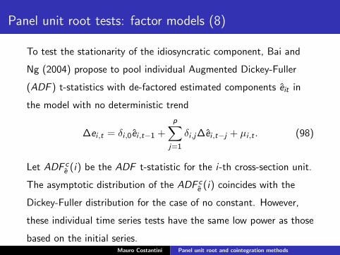
Panel unit root tests: factor models (8)
To test the stationarity of the idiosyncratic component, Bai and
Ng (2004) propose to pool individual Augmented Dickey-Fuller
(ADF ) t-statistics with de-factored estimated components eit in
the model with no deterministic trend
∆ei ,t = δi ,0ei ,t−1 +
p∑
j=1
δi ,j∆ei ,t−j + µi ,t . (98)
Let ADF ce (i) be the ADF t-statistic for the i-th cross-section unit.
The asymptotic distribution of the ADF ce (i) coincides with the
Dickey-Fuller distribution for the case of no constant. However,
these individual time series tests have the same low power as those
based on the initial series.Mauro Costantini Panel unit root and cointegration methods

Panel unit root tests: factor models (9)
Bai and Ng (2004) propose pooled tests based on Fisher type
statistics defined as in Choi (2001) and Maddala and Wu (1999).
Let Pce (i) be the p-value of the the ADF t-statistics for the i-th
cross-section unit, ADF ce (i), then the standardized Choi’s type
statistics is:
Z ce =
−2∑N
i=1 log Pce (i)− 2N√
4N. (99)
The statistics (99) converge for (N, T →∞) to a standard normal
distribution.
Mauro Costantini Panel unit root and cointegration methods

Panel unit root tests: cross-section averages methods,
Pesaran (2007) (1)
Pesaran proposed to augment the standard DF (or ADF)
regression with the cross section averages of lagged levels and
first-differences of the individual series.
If residuals are not serially correlated, the regression used for the
ith country is defined as:
∆yit = αi + ρiyi ,t−1 + ci yt−1 + di∆yt + eit . (100)
where yt−1 = (1/N)∑N
i=1 yit−1 and ∆yt = (1/N)∑N
i=1 ∆yit
Mauro Costantini Panel unit root and cointegration methods

Panel unit root tests: cross-section averages methods (2)
Let us denote ti (N, T ) the t-statistic of the OLS estimate of ρi .
The Pesaran’s test is based on these individual cross-sectionally
augmented ADF statistics, denoted CADF. A truncated version,
denoted CADF∗, is also considered to avoid undue influence of
extreme outcomes that could arise for small T samples.
Mauro Costantini Panel unit root and cointegration methods

Panel unit root tests: cross-section averages methods (3)
In both cases, the idea is to build a modified version of IPS t-bar
test based on the average of individual CADF or CADF∗ statistics
(respectively denoted CIPS and CIPS):
CIPS(N, T ) = N−1N∑
i=1
ti (N, T ) (101)
CIPS∗(N, T ) = N−1N∑
i=1
t∗i (N, T ) (102)
Mauro Costantini Panel unit root and cointegration methods

Panel unit root tests: cross-section averages methods (4)
where the truncated CADF statistics is defined:
t∗i (N, T ) =
K1 if ti (N, T ) ≤ K1
ti (N, T ) if K1 < ti (N,T ) < K2
K2 if ti (N, T ) ≥ K2
(103)
The constants K1 and K2 are fixed such that the probability that
ti (N, T ) belongs to [K1, K2] is near to one. In a model with
intercept only, the corresponding simulated values are respectively
-6.19 and 2.61
Mauro Costantini Panel unit root and cointegration methods

Panel unit root tests: cross-section averages methods (5)
Pesaran consider also the case of serially correlated residuals. For
an AR(p) error specification, the relevant individual CADF
statistics are computed from a pth order cross-section/time series
augmented regression:
∆yit = αi + ρiyi ,t−1 + ci yt−1 +
p∑
j=0
di ,j∆yt +
p∑
j=0
βi ,j∆yit−j + µit .
(104)
Mauro Costantini Panel unit root and cointegration methods

Cointegration tests: cross-section dependence(1)
Gengenbach, Palm and Urbain (2006) propose the following
testing procedure which consist of two steps:
1. A preliminary PANIC analysis on each variable Xi ,t and Yi ,t to
extract common factors is conducted. Tests for unit roots are
performed on both the common factors and the idiosyncratic
components using by Bai and Ng (2004) procedure.
Mauro Costantini Panel unit root and cointegration methods
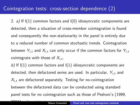
Cointegration tests: cross-section dependence (2)
2. a) If I(1) common factors and I(0) idiosyncratic components are
detected, then a situation of cross-member cointegration is found
and consequently the non-stationarity in the panel is entirely due
to a reduced number of common stochastic trends. Cointegration
between Yi ,t and Xi ,t can only occur if the common factors for Yi ,t
cointegrate with those of Xi ,t .
b) If I(1) common factors and I(1) idiosyncratic components are
detected, then defactored series are used. In particular, Yi ,t and
Xi ,t are defactored separately. Testing for no-cointegration
between the defactored data can be conducted using standard
panel tests for no cointegration such as those of Pedroni’s (1999,
2004) unit root tests.Mauro Costantini Panel unit root and cointegration methods

Panel estimation: cross-sectional dependence (1)
Bai and Kao (2006) consider the following fixed-effect panel
regression:
yit = αi + x′itβ + eit i = 1, ...,N, t = 1, ...,T , (105)
where yit are 1× 1, β is a k × 1 vector of the slope parameters,
αi are the intercepts, and eit are the stationary disturbance
terms. They assumed that xit is K × 1 integrated processes of
order one for all i, where
xit = xit−1 + εit .
Under these specifications, the previous equation defines a system
of cointegrated regressions, i.e. yit is cointegrated with xit .Mauro Costantini Panel unit root and cointegration methods
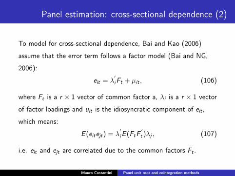
Panel estimation: cross-sectional dependence (2)
To model for cross-sectional dependence, Bai and Kao (2006)
assume that the error term follows a factor model (Bai and NG,
2006):
eit = λ′iFt + µit , (106)
where Ft is a r × 1 vector of common factor a, λi is a r × 1 vector
of factor loadings and uit is the idiosyncratic component of eit ,
which means:
E (eitejt) = λ′iE (FtF
′t )λj , (107)
i.e. eit and ejt are correlated due to the common factors Ft .
Mauro Costantini Panel unit root and cointegration methods

Panel estimation: cross-sectional dependence (3)
The OLS estimator of β is :
βOLS =
[ N∑
i=1
T∑
t=1
yit(xit − xi )′][ N∑
i=1
T∑
t=1
(xit − xi )(xit − xi )′]−1
(108)
As regards the limiting distribution, we have:
√nT
(βOLS − β
)−√nδnT ⇒ N
(0, 6Ω−1
ε AΩ−1ε
)(109)
as (n,T →∞), with nT → 0,
Mauro Costantini Panel unit root and cointegration methods

Panel estimation: cross-sectional dependence (4)
where
A = limn→∞
1
n
n∑
i=1
(λ′iΩF .εiλiΩεi + Ωµ.εiΩεi
)
and
δnT =1
n
[ n∑
i=1
λ′i
(ΩFεiΩ
1/2εi
(∫WidW
′i
)Ω−1/2εi + ∆Fεi
)+
ΩµεiΩ1/2εi
(∫WidW
′i
)Ω−1/2εi + ∆µεi
]×
[1
n
N∑
i=1
T∑
t=1
1
T 2(xit − xi )(xit − xi )
′]−1
Mauro Costantini Panel unit root and cointegration methods

Panel estimation: cross-sectional dependence (5)
and
Wi = Wi −∫
Wi , andΩε = limn→∞
1
n
n∑
i=1
Ωεi
and
Ωi =
ΩFi ΩFµi ΩFei
ΩµFi Ωµi Ωµεi
ΩεFi Ωεµi Ωεi
(110)
Mauro Costantini Panel unit root and cointegration methods
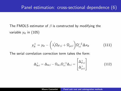
Panel estimation: cross-sectional dependence (6)
The FMOLS estimator of β is constructed by modifying the
variable yit in (105)
y+it = yit −
(λ′iΩFεi + Ωµεi
)Ω−1
εi ∆xit (111)
The serial correlation correction term takes the form:
∆+bεi = ∆bεi − ΩbεiΩ
−1εi ∆εi =
∆+
Fεi
∆+µεi
(112)
Mauro Costantini Panel unit root and cointegration methods

Panel estimation: cross-sectional dependence (7)
The infeasible estimator is:
βFM =
[ N∑
i=1
( T∑
t=1
y+it (xit − xi )
′ − T
(λ′i∆
+Fεi + ∆+
Fεi
))]
[ N∑
i=1
T∑
t=1
(xit − xi )(xit − xi )′]−1
(113)
Mauro Costantini Panel unit root and cointegration methods

Panel estimation: cross-sectional dependence (8)
The limiting distribution of the infeasible estimator is:
√nT
(βFM − β
)⇒ N
(0, 6Ω−1
ε CΩ−1ε
)(114)
as (n, T →∞), with nT → 0,
where
A = limn→∞
1
n
n∑
i=1
(λ′iΩF .εiλiΩεi + Ωµ.εiΩεi
)
Mauro Costantini Panel unit root and cointegration methods

Panel estimation: cross-sectional dependence (9)
The feasible FMOLS is obtained by substituting λi , Ft , σi and Ωi ,
with λi , Ft , σi and Ωi , The asymptotic distribution is:
√nT
(βFM − βFM
)⇒ 1
n√
T
n∑
i=1
( t∑
i=1
e+it (xit − xi )
′)− T ∆+
bεn
)−
( t∑
i=1
e+it (xit − xu)
′)− T∆+
bεn
)
=
[1
n√
T
n∑
i=1
( t∑
i=1
(e+it − e+
it )(xit − xi )′)− T (∆+
bεn −∆+bεn
)]
[1
nT 2
n∑
i=1
t∑
i=1
(xit − xi )(xit − xi )−1
]−1
(115)
as (n,T →∞), with nT → 0,Mauro Costantini Panel unit root and cointegration methods

Panel estimation: cross-sectional dependence
(10)
In the literature, the FM-type estimators usually were computed
with a two-step procedure, by assuming an initial consistent of β,
say βOLS . Then, one can constructs estimates of the long-run
covariance matrix, Ω(1), and loading, λ(1)i . The 2S-FM, denoted by
β2S , is obtained using Ω(1) and λ(1)i :
β(1)2S =
[ N∑
i=1
( T∑
t=1
y+(1)it (xit − xi )
′ − T
(λ′(1)i ∆
+(1)Fεi + ∆
+(1)Fεi
))]
[ N∑
i=1
T∑
t=1
(xit − xi )(xit − xi )′]−1
(116)
Mauro Costantini Panel unit root and cointegration methods

Panel estimation: cross-sectional dependence
(10)
Bai and Kao (2006) propose the CUP-FM estimator. The
CUP-FM estimator is constructed by estimating parameters,
long-run covariance matrix an loading recursively. Thus βFM , Ω(1)
and λ(1)i are estimated repeatedly, until convergence is reached.
Mauro Costantini Panel unit root and cointegration methods

Panel estimation: cross-sectional dependence
(11)
The CUP-FM estimator is defined as:
βCUP =
[ N∑
i=1
( T∑
t=1
y+(1)it (βCUP)(xit − xi )
′
−T
(λ′i
(βCUP
)∆+
Fεi
(βCUP
)+ ∆+
Fεi
(βCUP
)))]
[ N∑
i=1
T∑
t=1
(xit − xi )(xit − xi )′]−1
(117)
Mauro Costantini Panel unit root and cointegration methods