1

Paper for AIAA Joint Propulsion Conference, July 27-29, 2015, Orlando, Florida

Use of Generalized Fluid System Simulation Program (GFSSP) for Teaching

and Performing Senior Design Projects at the Educational Institutions

A. K. Majumdar and A. Hedayat

Propulsion Systems Department

Marshall Space Flight Center, MSFC, AL 35812

Abstract

This paper describes the experience of the authors in using the Generalized Fluid System

Simulation Program (GFSSP) in teaching Design of Thermal Systems class at University

of Alabama in Huntsville. GFSSP is a finite volume based thermo-fluid system network

analysis code, developed at NASA/Marshall Space Flight Center, and is extensively used

in NASA, Department of Defense, and aerospace industries for propulsion system design,

analysis, and performance evaluation. The educational version of GFSSP is freely

available to all US higher education institutions. The main purpose of the paper is to

illustrate the utilization of this user-friendly code for the thermal systems design and fluid

engineering courses and to encourage the instructors to utilize the code for the class

assignments as well as senior design projects.

1. Introduction

There is increasing use of computational tools for design and analysis in thermal and fluid

engineering industries. The engineers fresh from school are generally proficient with the

use of software for writing reports or preparing presentations. However, they receive very

little training on thermal and fluid analysis software in undergraduate program. One of the

reason for such deficiency is the lack of availability of the software that can be integrated

with the engineering course. Many of these software are commercial and universities may

not have the resources for licensing these software. To fill this gap, NASA/Marshall Space

Flight Center have developed an educational version of Generalized Fluid System

Simulation Program (GFSSP) which is available free of cost for classroom use in

engineering universities at United States.

GFSSP is a finite volume based flow network analysis software. Finite Volume Method

(FVM) is extensively used in Computational Fluid Dynamics (CFD) to solve Navier-

Stokes equation. Many commercial CFD codes (FLUENT, CFX, and FLOW3D) are based

on FVM. FVM is an extension of the control volume analysis technique of classical

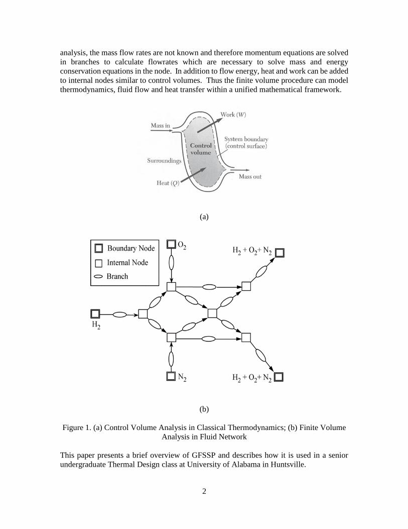
thermodynamics. In Figure 1a, a typical control volume is shown for mass and energy

conservation based on the first law of thermodynamics. Finite volume analysis of fluid

network is shown in Figure 1b. A fluid network consists of boundary nodes, internal nodes

and branches. Boundary and internal nodes are connected through branches in series or

parallel arrangements. Mass and energy conservation equations are solved in internal

nodes similar to control volumes of classical thermodynamics. Flowrates are calculated in

branches. In control volume analysis, mass flow rates are known. In finite volume

https://ntrs.nasa.gov/search.jsp?R=20150016530 2018-07-08T16:40:31+00:00Z

2

analysis, the mass flow rates are not known and therefore momentum equations are solved

in branches to calculate flowrates which are necessary to solve mass and energy

conservation equations in the node. In addition to flow energy, heat and work can be added

to internal nodes similar to control volumes. Thus the finite volume procedure can model

thermodynamics, fluid flow and heat transfer within a unified mathematical framework.

(a)

(b)

Figure 1. (a) Control Volume Analysis in Classical Thermodynamics; (b) Finite Volume

Analysis in Fluid Network

This paper presents a brief overview of GFSSP and describes how it is used in a senior

undergraduate Thermal Design class at University of Alabama in Huntsville.

3

2. GFSSP Overview

In GFSSP, a fluid circuit is constructed with boundary nodes, internal nodes and branches

(Figure 1b) while the solid circuit is constructed with solid nodes, ambient nodes and

conductors. The solid and fluid nodes are connected with solid-fluid conductors. Users

must specify conditions, such as pressure, temperature and concentration of species at the

boundary nodes. These variables are calculated at the internal nodes by solving

conservation equations of mass, energy and species in conjunction with the thermodynamic

equation of state. Each internal node is a control volume where there are inflow and

outflow of mass, energy and species at the boundaries of the control volume. The internal

node also has resident mass, energy and concentration. The momentum conservation

equation is expressed in flowrates and is solved in branches. At the solid node, the energy

conservation equation for solid is solved to compute temperature of the solid node. Figure

2 shows a schematic and GFSSP flow circuit of a counter-flow heat exchanger. Hot

nitrogen gas is flowing through a pipe, colder nitrogen is flowing counter to the hot stream

in the annulus pipe and heat transfer occurs through metal tubes. The problem considered

is to calculate flowrates and temperature distributions in both streams.

Nitrogen 250 º F

Nitrogen 70 º F Dinner= 2 inches

Douter= 4 inches

L= 2 ft

2.59 lb/sm

2.63 lb/sm

Internal Node

Boundary Node

Solid

Node

Solid-Fluid

Conductor

Solid-Solid

Conductor

4

Figure 2. A Typical Flow Network consists of Fluid Node, Solid Node, Flow

Branches and Conductors

GFSSP has a unique data structure shown in Figure 3; this allows constructing all possible

arrangements of a flow network with no limit on the number of elements. The elements of

a flow network are boundary nodes where pressure and temperature are specified, internal

nodes where pressure and temperature are calculated, and branches where flowrates are

calculated. For conjugate heat transfer problems, there are three additional elements: solid

node, ambient node, and conductor. The solid and fluid nodes are connected with solid-

fluid conductors.

Figure 3. Data structure of the fluid-solid network has six major elements.

The mathematical closure is described in Table 1. GFSSP uses a pressure based scheme as

pressure is computed from mass conservation equation. The mass and momentum

conservation equations and thermodynamic equation of state are solved simultaneously by

the Newton-Raphson method while energy conservation equations of fluid and solid are

solved separately but implicitly coupled with the other equations stated above. Further

details of the mathematical formulation and solution procedure are described in reference

1.

GFSSP is linked with two thermodynamic property programs, GASP2 and WASP3 and

GASPAK4, that provide thermodynamic and thermophysical properties of selected fluids.

Both programs cover a range of pressure and temperature that allows fluid properties to be

evaluated for liquid, liquid-vapor (saturation), and vapor region. GASP and WASP provide

properties of 12 fluids. GASPAK includes a library of 36 fluids.

5

Table 1. Mathematical Closure

Unknown Variables Available Equations to Solve

1. Pressure 1. Mass Conservation Equation

2. Flowrate 2. Momentum Conservation Equation

3. Fluid Temperature 3. Energy Conservation Equation of Fluid

4. Solid Temperature 4. Energy Conservation Equation of Solid

5. Fluid Mass (Unsteady Flow) 5. Thermodynamic Equation of State

GFSSP has three major parts. The first part is the graphical user interface (GUI), visual

thermofluid analyzer of systems and components (VTASC). VTASC allows users to create

a flow circuit by a ‘point and click’ paradigm. It creates the GFSSP input file after the

completion of the model building process. GFSSP’s GUI provides the users a platform to

build and run their models. It also allows post-processing of results. The network flow

circuit is first built using three basic elements: boundary node, internal node, and branch.

Figure 4 - GFSSP’s Program Structure showing the interaction of three major

modules

3. Utilization of GFSSP in Senior Design Project

Utilization of GFSSP has been incorporated in the syllabus of Design of Thermal Systems

course, a senior level class, at the University of Alabama in Huntsville. The utilization of

GFSSP includes tutorials, homework assignments, and a design project. For the design

project, the class divided into multiple teams, each having 3 or 4 team members. The

students were encouraged to form and select a team lead who oversaw overall progress of

6

the project. Each team is required to submit a project report and make a presentation. A

tutorial example and brief review of the design project assignment submitted by one of the

team are presented in the following sections.

3.1 Tutorial Example: Pressurization of a Propellant Tank

This example demonstrates the use of GFSSP’s unsteady formulation by predicting the

pressure and temperature history during the blowdown of a pressurized tank. A schematic

of a propellant pressurization system is shown in Figure 5. It is assumed that initially the

ullage, space is filled with pressurant, helium (He), at propellant temperature. As the warm

pressurant enters the ullage space, it mixes with the cold ullage gas and the temperature of

the ullage gas starts to increase due to mixing and compression. Initially, the walls of the

tank are also at propellant temperature. Heat transfer from the ullage gas to the propellant,

liquid oxygen (LOX), and the tank wall and mass transfer from the propellant to the ullage

start immediately after the pressurant begins flowing into the tank. Propellant flows from

the tank to the engine under the influence of ullage pressure and gravitational head in the

tank. In this model, condensation of propellant vapor has been neglected.

Figure 5. Schematic of propellant tank pressurization system.

GFSSP Model

A five-node pressurization system, as shown in Figure 6(a), was developed. Helium at 95

psia and 120 ºF enters the ullage space, which is initially filled with helium at 67 psia and

–264 ºF. Node 2 represents the ullage space, which has an initial volume of 25 ft3. A pseudo

boundary node (node 3) has been introduced to exert ullage pressure on the initial

propellant volume of 475 ft3, which is represented by node 4. The pressure at the pseudo

boundary node is calculated from the ullage pressure and gravitational head and is the

driving force to supply the propellant to the engine. This pressure is calculated at the

beginning of each time step. Branch 12 models the tank inlet, branch 34 represents the

7

propellant surface, and branch 45 represents the line to the engine. All three branches were

modeled using a Flow Through a Restriction. The flow coefficient of branch 45 is adjusted

to restrict the propellant flow such that all propellant is expelled from the tank over the

course of the run. In this test model, the engine inlet pressure was set at 50 psia. Figure

6(b) shows how the model looks in VTASC. Figure 7 shows the VTASC tank

pressurization dialog and inputs for example 10.

Figure 6. Simple pressurization system test model: (a) Detailed model schematic

and (b) VTASC model.

Results and Discussions

The pressurization system transient test model was run for 200 seconds (s) with 0.1s time

step. Figure 7 shows both the ullage pressure and tank bottom pressure histories for the test

model. After an initial pressure rise due to a ‘ramping up’ transient effect, both pressures

begin a slow but steady decline for the remainder of the run. It should be noted that tank

bottom pressure was calculated by adding ullage pressure with pressure due to the

gravitational head. Figure 7 shows that as the gravitational head decreases, the ullage and

tank bottom pressures slowly converge until all propellant is drained from the tank. The

slow decline in ullage pressure is mainly due to the expanding ullage volume.

Figure 8 shows the histories for the ullage temperature and the tank wall temperature. This

figure shows that the tank wall temperature rises 32 ºF over the course of the model run. It

8

reveals that the 120 ºF helium gas entering the tank has an increasing effect on the tank

wall as propellant is drained from the tank and the wall surface area exposed to the warmer

ullage gas grows. This effect is somewhat dampened, however, because the heat gained by

the wall is conducted to the portion of the tank that is submerged in LOX, which acts as a

heat sink. The ullage temperature rises 192 ºF during the first 60 seconds of tank

pressurization before beginning a slow decline for the remainder of the simulation. This

large initial temperature rise is primarily due to the mixing of hot helium gas with the

relatively cold gas present in the ullage. The decline in temperature is a result of expansion

due to a continuous increase of the ullage volume.

Figure 7. Ullage and tank bottom Figure 8. Ullage and tank wall

pressure history. temperature history.

Helium flow rate into the tank is shown in Figure 9. The helium flow rate was found to

drop initially as the start transient takes place, which is consistent with the ‘ramp up’ effect

noted in Figure 7. Then the flow rate begins to gradually increase as ullage pressure drops

due to the expanding ullage volume. LOX flow rate into the engine is shown in Figure 10.

The LOX flow rate curve mirrors the ullage and tank bottom pressure curves, rising through

an initial start transient to a peak value and then declining for the remainder of the run as

tank pressure drops.

Figure 9. Helium mass flow rate history. Figure 10. LOX mass flow rate history.

9

3.2 Design Project Assignment

The objective of the design project was to develop a design for a chilled-water air-

conditioning system. This design supplies water from a chiller to air handling units (AHUs)

in a four-story office complex, and meets design requirements set forth in the design project

description. These requirements govern the flow rates in different branches of the system,

the maximum allowable velocity through the pipes, the pressure drops across components,

and the pipe length. In chilled-water air-conditioning systems water is pumped through a

chiller, into a network of pipes that supply water to the AHUs. Air is passed through the

AHUs and the chilled water extracts heat from the air, cooling the airflow, which is then

distributed to the different rooms on the floor. These air conditioning systems are

commonly used in large buildings, such as hotels or office complexes, where each floor

has its own AHU, allowing different floors to be cooled individually. The basic flow circuit

is shown in Figure 11. The “P” component represents the pump, and the “C” component

represents the chiller.

Figure 11. Basic flow circuit shown in project requirements.

Design Requirements

Several design requirements had to be met for this chilled-water flow network, which are

outlined in Table 2. These requirements specify flow rates, flow velocities, pressure

drops, and pipe lengths. For the prescribed requirements, several quantities had to be

determined. These quantities were:

1. Floor pipe size

2. Supply and return pipe size

3. Pressure rise across the pump

4. Pump horsepower for an efficiency of 55%

5. Cost to operate the system for a day, assuming a price of $0.10 per KW-hr

10

Requirement

Number Title Description

1 Flow Rate Each floor requires a chilled-water flow

rate of 18,000 lbm/hr

2 Flow Velocities All flow velocities are not to exceed 5 ft/s

3 Floor Spacing Each floor is 12 feet higher than the one

below

4 Supply and Return

Pipe Sizing

The supply and return pipes must all be

the same diameter (Schedule 80)

5 Supply Pipe Length

The total length of supply pipe running

from the exit of the bottom floor, through

the pump and chiller, and up to the

entrance of the top floor is 300 feet. (See

Figure #1).

6 Floor Pipe Sizing The floor pipes must all be the same

diameter (Schedule 80)

7 Floor Pipe Length Each floor must have 100 feet of pipe

8 Floor Valves Each floor must have two gate valves

9 Air Handling Unit

Pressure Drop

The pressure drop across each AHU must

be 50 psi

10 Chiller Pressure

Drop

The pressure drop across the chiller must

be 100 psi

Table 2: Air-Conditioning System Requirements.

Assumptions

1. Neglected losses due to couplings/welds required to join sections of steel pipe,

which typically come in 10-12 foot lengths, to obtain the lengths specified in the

problem (100 feet of 2” and 300 feet of 4”, etc).

2. Assumed a <0.5% deviation from values specified in project requirements was

acceptable.

GFSSP Model

The flow circuit, illustrated in Figure 11, was created in GFSSP and is shown in Figure

12.

11

Figure 12. GFSSP flow circuit with numbered nodes and branches.

GFSSP model simulation of the flow circuit yielded a set of design results for pipe sizes,

pressure drops, flow rates, flow velocities, required horsepower, and cost of operation.

These results are summarized in the Table 3, and demonstrate that the design fully meets

all project requirements. Overall, as seen from Table 3, after defining and/or solving for all

unknown quantities, the results of the design closely meet the design requirements. The

results of the GFSSP model are within 0.3% percent difference of the ideal design

requirements.

12

Table 3. Project Design Results.

4. Conclusions

This paper demonstrates how a system level, user friendly network flow analysis code

can be integrated in a senior level thermal design class. The intent was to introduce a

state of the art computational tool to perform a real world technical task. The

introduction of GFSSP was done through lectures, tutorials and senior design project.

The authors’ experience of using GFSSP in the class was very positive mainly due to

very positive feedback from students about their learning experience while performing

the project. GFSSP is available free of cost to all universities in the United States from

NASA/MSFC’s Technology Transfer Office.

13

Acknowledgement

This work was supported by National Institute of Rocket Propulsion (NIRPS) at NASA/

MSFC. The authors wish to thank the STI Publication Office of NASA/MSFC for the

preparation of this manuscript.

References

1. A.K. Majumdar, A.C. LeClair, R. Moore, P.A. Schallhorn, Generalized Fluid

System Simulation Program, Version 6.0, NASA/TM—2013–217492 (October

2013) <https://gfssp.msfc.nasa.gov>.

2. Hendricks, R.C.; Baron, A.K.; and Peller, I.C.: “GASP — A Computer Code for

Calculating the Thermodynamic and Transport Properties for Ten Fluids:

Parahydrogen, Helium, Neon, Methane, Nitrogen, Carbon Monoxide, Oxygen,

Fluorine, Argon, and Carbon Dioxide,” NASA TN D-7808, NASA Lewis Research

Center, Cleveland, OH, February 1975.

3. Hendricks, R.C.; Peller, I.C.; and Baron, A.K., “WASP - A Flexible Fortran IV

Computer Code for Calculating Water and Steam Properties,” NASA TN D-7391,

NASA Lewis Research Center Cleveland, OH, November 1973.

4. User’s Guide to GASPAK, Version 3.20, Cryodata, Inc., November 1994.