Classical and Quantum Gravity

PAPER • OPEN ACCESS

Post-Newtonian corrections to Schrödinger equations in gravitationalfieldsTo cite this article: Philip K Schwartz and Domenico Giulini 2019 Class. Quantum Grav. 36 095016

 

View the article online for updates and enhancements.

This content was downloaded from IP address 194.95.159.70 on 03/07/2019 at 12:00

1

Classical and Quantum Gravity

Post-Newtonian corrections to Schrödinger equations in gravitational fields

Philip K Schwartz1 and Domenico Giulini1,2

1 Institute for Theoretical Physics, Leibniz University Hannover, Appelstraße 2, 30167 Hannover, Germany2 Center of Applied Space Technology and Microgravity, University of Bremen, Am Fallturm 1, 28359 Bremen, Germany

E-mail: philip.schwartz@itp.uni-hannover.de and giulini@itp.uni-hannover.de

Received 14 December 2018, revised 25 February 2019Accepted for publication 14 March 2019Published 12 April 2019

AbstractIn this paper we extend the WKB-like ‘non-relativistic’ expansion of the minimally coupled Klein–Gordon equation after (Kiefer and Singh 1991 Phys. Rev. D 44 1067–76; Lämmerzahl 1995 Phys. Lett. A 203 12–7; Giulini and Großardt 2012 Class. Quantum Grav. 29 215010) to arbitrary order in c−1, leading to Schrödinger equations describing a quantum particle in a general gravitational field, and compare the results with canonical quantisation of a free particle in curved spacetime, following (Wajima et al 1997 Phys. Rev. D 55 1964–70). Furthermore, using a more operator-algebraic approach, the Klein–Gordon equation and the canonical quantisation method are shown to lead to the same results for some special terms in the Hamiltonian describing a single particle in a general stationary spacetime, without any ‘non-relativistic’ expansion.

Keywords: quantum matter in gravity, non-relativistic expansion, post-Newtonian expansion, Klein–Gordon equation, formal WKB expansion

1. Introduction

Suppose we are given a quantum-mechanical system whose time evolution in the absence of gravity is known in terms of the ordinary time-dependent Schrödinger equation. In other words: we know the system’s Hamiltonian if all gravitational interactions are neglected. We ask: what principles do we use in order to deduce the system’s interaction with a given exter-nal gravitational field? Note that by ‘gravitational field’ we understand all the ten components

P K Schwartz and D Giulini

Post-Newtonian corrections to Schrödinger equations in gravitational fields

Printed in the UK

095016

CQGRDG

© 2019 IOP Publishing Ltd

36

Class. Quantum Grav.

CQG

1361-6382

10.1088/1361-6382/ab0fbd

Paper

9

1

26

Classical and Quantum Gravity

IOP

Original content from this work may be used under the terms of the Creative Commons Attribution 3.0 licence. Any further distribution of this work must maintain attribution to the author(s) and the title of the work, journal citation and DOI.

2019

1361-6382/19/095016+26$33.00 © 2019 IOP Publishing Ltd Printed in the UK

Class. Quantum Grav. 36 (2019) 095016 (26pp) https://doi.org/10.1088/1361-6382/ab0fbd

2

gµν of the spacetime metric that are subject to Einstein’s field equations of general relativity (or, more generally, to the equations of some other metric theory of gravity), not just the scalar component φ representing the Newtonian potential.

The behaviour of quantum systems in general gravitational fields is naturally of fundamen-tal interest, relating, e.g. to the reaction of quantum systems to gravitational waves [5], tests of general relativity, the controversially discussed topic of gravitationally induced quant um dephasing [6–8], quantum tests of the classical equivalence principle [9] or proposals of quant um formulations of the equivalence principle [10] and tests thereof [11].

The conceptual difficulty we are addressing here has to do with the fact that the usual ‘minimal coupling scheme’ that we usually employ in order to couple any classical field obey-ing Lorentz invariant equations of motion simply does not apply to the case at hand. We recall that, in a nutshell, this prescription is a two step process: (1) Write down the matter’s dynami-cal law in a Poincaré invariant fashion in Minkowski spacetime; (2) replace the flat Minkowski metric η by a general Lorentzian metric g and the partial derivatives with respect to the affine coordinates of Minkowski spacetime (i.e. the covariant derivatives with respect to η) by the Levi-Civita covariant derivative with respect to g.

This procedure suffers from an essential non-uniqueness which has to do with the fact that the covariant derivatives with respect to η commute whereas those with respect to g gener-ally do not. Hence there are equivalent forms for the dynamical laws in step (1) that turn into inequivalent extensions after performing step (2). The differences will consist in terms that result from commuting covariant derivatives and hence in local couplings of g’s curvature tensor to the matter field. Modulo this well known ambiguity the prescription just outlined is straightforward to apply and has been successfully used in all applications of general relativity.

The point addressed here in connection with quantum mechanics is not so much the ambi-guity just described, but rather the obvious failure to even implement step (1): there simply is no obvious way to rewrite the Schrödinger equation into a Poincaré invariant form in order to be able to apply step (2). Special relativity turns quantum mechanics into relativistic quant um field theory (RQFT) in which the particle concept ceases to be meaningful in presence of general background geometries [12, 13]. Does that mean we would have to employ the whole machinery of RQFT in order to just answer simple questions concerning matter-gravity inter-actions that go beyond the simplest (and obvious; see below) couplings to the Newtonian potential? We think the answer is no, but at the same time we think that the alternative should not result in ad hoc procedures guided by more or less well founded ‘physical intuition’. Rather we should look for a general and systematic method that allows to derive the full coupling by means of an algorithm that arguably qualifies as a proper post-Newtonian approx-imation. We see this paper as a positive contribution to this end.

To be slightly more precise, we recall that the Schrödinger equation describing a ‘non-relativistic’ (i.e. not Poincaré invariant) particle of mass m and zero spin in a background Newtonian gravitational field with potential φ is

i�∂tψ =

(− �2

2m∆+ mφ

)ψ. (1.1)

This equation has extensively been tested in the gravitational field of the earth, beginning with neutron interferometry in the classic COW experiment [14] and leading up to atom inter-ferometers of the Kasevich–Chu type, accomplishing, e.g. highly precise measurements of the gravitational acceleration g on the earth [15]. We now ask what kind of ‘post-Newtonian corrections’ to this equation arise from general relativity or other metric theories of gravity,

P K Schwartz and D Giulini Class. Quantum Grav. 36 (2019) 095016

3

considering additional terms involving the Newtonian potential φ as well as new terms involv-ing all ten metric components gµν.

In the existing literature, one finds two different main approaches to this problem of post-Newtonian correction terms for the Schrödinger equation describing a particle in a curved spacetime. The first, described, e.g. by Wajima et al [4], starts from a classical description of the particle and applies canonical quantisation rules adapted to the situation (in a somewhat ad hoc fashion) to derive a quantum mechanical Hamiltonian. By an expansion in powers of c−1 (at the stage of the classical Hamiltonian), one finds the desired correction terms. Other methods along a similar line use path integral quantisation on the classical system, as, e.g. the semi-classical calculation by Dimopoulos et al [16].

The second, fundamentally different approach takes a field-theoretic perspective and derives the Schrödinger equation as an equation for the positive frequency solutions of the minimally coupled classical Klein–Gordon equation3. This is accomplished by Kiefer and Singh [1], Lämmerzahl [2] and Giulini and Großardt [3] by making a WKB-like ansatz for the Klein–Gordon field and thus (formally) expanding the Klein–Gordon equation in powers of c−1, in the end viewing the Klein–Gordon theory as a (formal) deformation of the Schrödinger theory, implementing the deformation of Galilei to Poincaré symmetry well-known at the level of Lie algebras [17]. This second method seems to be more firmly rooted in first prin-ciples than the canonical quantisation method, since it can at least heuristically be motivated from quantum field theory in curved spacetimes (see section 3.1).

The calculation of general-relativistic corrections to phase shifts in atom interferometry by Dimopoulos et al [16] used a semi-classical approximation scheme, the so-called ‘stationary phase approximation’ in path integral terms, which is non-exact for Hamiltonians of higher than quadratic order in positions and momenta. The approximation breaks down for wave packets with large width in phase space, so that similar methods cannot directly be applied when considering the effect of general gravitational fields on, e.g. large spatial superpositions, for example proposed relevant for gravitational dephasing by Pikovski et al [6]. In contrast to this, using a modified Schrödinger equation  makes it possible to, in principle, describe quant um systems under gravity without any semi-classical approximation.

Although the two methods for obtaining post-Newtonian Schrödinger equations described above are very different in spirit, they lead to comparable results in lowest orders. To make possible a general comparison beyond the explicit examples considered in the existing litera-ture4, we will apply the methods to as general a metric as possible: in section 2, we will give a brief overview over the canonical quantisation method, while section 3 will develop the WKB-like formal expansion of the Klein–Gordon equation to arbitrary order in c−1 in a general met-ric given as a formal power series in c−1, significantly extending existing explicit examples to the general case. This leads to some simple comparisons of the resulting Hamiltonian with the one from canonical quantisation.

In section 4, we consider a (formal) expansion of the Klein–Gordon equation in powers of momentum operators leading to a Schrödinger form of the equation, yielding some general statements about similarities between the canonical and the Klein–Gordon methods without any ‘non-relativistic’ expansion in powers of c−1.

A general WKB-like ‘non-relativistic’ formal expansion of the Klein–Gordon equation to obtain a Schrödinger equation was already considered by Tagirov in [18] and a series of fol-low-up papers [19, 20], as summarised in [21]; but unlike our approach, these works did not

3 For simplicity we call, as is common, the Poincaré invariant mass m and zero-spin equation by the names of Oskar Klein and Walter Gordon, even though Erwin Schrödinger and Vladimir Fock were amongst the first to consider it.4 Wajima et al [4] considered a first-order post-Newtonian metric for a point-like rotating source, Lämmerzahl [2] used a first-order Eddington–Robertson PPN metric.

P K Schwartz and D Giulini Class. Quantum Grav. 36 (2019) 095016

4

expand the metric, thus not allowing to directly apply the results to metrics given as a power series in c−1. Tagirov also compared his WKB-like approach to methods of canonical quanti-sation [22], but did this only for the case of static metrics.

We will use the ‘mostly plus’ signature convention for the spacetime metric, i.e. (−,+,+,+). Since we are concerned mostly with conceptual questions, we will generally not be mathematically very rigorous, and in particular not mention domains of definition of operators.

2. Canonical quantisation of a free particle

In the following, we will describe the canonical quantisation approach used by Wajima et al [4] to derive a Hamiltonian for a quantum particle in the post-Newtonian gravitational field of a point-like rotating source for the analysis of effects on interferometric phase shifts. We will focus on the conceptual issues of the procedure since we want to stay as general as possible.

The classical action for a ‘relativistic’ point particle of mass m in curved spacetime with metric g is

S = −mc∫ √

−g(x′(λ), x′(λ))dλ = −mc∫ √

−gµνx′µx′νdλ, (2.1)

where x(λ) is the arbitrarily parametrised worldline of the particle.We assume the spacetime to be globally hyperbolic and perform a 3 + 1 decomposition

of spacetime [23]: we foliate spacetime M into 3-dimensional spacelike Cauchy surfaces Σt which are images of an ‘abstract’ Cauchy surface Σ under a family of embeddings Et : Σ → M , parametrised by a ‘foliation parameter’ t ∈ R, and we introduce spacetime coordinates such that xi are coordinates on Σ and x0 = ct. Parametrising the worldline of the particle by t, the classical Hamiltonian can be computed to be

H =1√−g00

c[

m2c2 +

(gij − 1

g00 g0ig0j)

pipj

]1/2

+c

g00 g0ipi, (2.2)

when expressed in terms of the spacetime metric, where p i are the momenta conjugate to xi. Full details of this calculation can be found in appendix A.

Now, we want to ‘canonically quantise’ this Hamiltonian. To this end, we have to define a Hilbert space for our quantum theory, define position and momentum operators acting on this Hilbert space and satisfying the canonical commutation relations, and choose an operator ordering scheme for symmetrising products of momenta and (functions of) position. By then expanding the square root in the classical Hamiltonian (2.2) to the desired order in c−1 (or in momenta, see section 4) and afterwards replacing the classical momentum and position vari-ables by the corresponding operators, applying the chosen ordering scheme, we get a quanti-sed Hamiltonian H acting on our Hilbert space and can postulate a Schrödinger equation in the usual form

i�∂tψ = Hψ. (2.3)

Let us stress once more that this Hamiltonian will depend not only on the choice of 3 + 1 decomposition of spacetime into Cauchy surfaces, which is the case since for a post-Newto-nian approximation we need some notion of separate space and time, but also on the choice of operator ordering scheme, which we leave open in order to keep the discussion as general as possible.

P K Schwartz and D Giulini Class. Quantum Grav. 36 (2019) 095016

5

We now turn to the definition of the Hilbert space and the position and momentum opera-tors, which is more subtle than might be anticipated at first thought. Since the position vari-ables in the classical Hamiltonian (2.2) are the spatial coordinates xi on the Cauchy surfaces, we want the quantum position operators to directly correspond to these. Thus, we want to define the Hilbert space as some space of square-integrable ‘wavefunctions’ of the xi, such that we can take as position operators simply the operators of multiplication with the coordinates. The question of definition of the Hilbert space thus becomes a question of choice of a scalar product on (some subspace of) the space of functions of the xi.

To be more precise, we do not just need a single Hilbert space: to any ‘time’ (i.e. foliation parameter) t we want to associate a wavefunction ψ(t) giving rise to a position probability distribution on the Cauchy surface Σt corresponding to t, so we need to consider an individual Hilbert space for each Cauchy surface in the 3 + 1 decomposition. But since we want to relate these wavefunctions by a Schrödinger equation, we have to somehow identify the Hilbert spaces corresponding to the different Cauchy surfaces, which we are now going to explain.

A natural, geometric choice of scalar product on the space of functions on Σt is the L2-sca-lar product with respect to the induced metric measure (see [4]), i.e.

〈ψ,ϕ〉Σt :=∫

ψϕ√

(3)g|Σt d3x, (2.4)

where here and in the following, we write (3)g = det(gij). Consider first the case that the spa-tial metric gij be independent of t, i.e. that the induced geometry be the same for all Cauchy surfaces. Then this scalar product is independent of t, such that the Hilbert spaces corre-sponding to the different Cauchy surfaces are canonically identified by simply identifying the wavefunctions5. We can then define the momentum operator as

pi := −i�(3)g−1/4∂i((3)g1/4·), (2.5)

which is symmetric with respect to the scalar product and fulfils the canonical commutation relation [xi, pj] = i�δi

j , and carry out canonical quantisation as described above.If we allow for gij to depend on t, the scalar product (2.4) depends on t and thus the canonical

map L2(Σ, 〈·, ·〉Σt) � ψ �→ ψ ∈ L2(Σ, 〈·, ·〉Σs) no longer is an isomorphism of Hilbert spaces. I.e. the natural identification from above does not work, spoiling the program of canonical quantisation. A natural solution to this problem is to instead consider the time-independent ‘flat’ L2-scalar product

〈ψf ,ϕf 〉f :=∫

ψfϕf d3x (2.6)

together with the ‘flat’ momentum operator pi := −i�∂i. Using these, canonical quantisation can be carried out. At first sight, this scalar product could seem less ‘geometric’ than (2.4), but it can be seen to have as much invariant meaning as the latter by realising that, geometri-cally speaking, the ‘flat’ wavefunctions ψf ,ϕf be scalar densities (of weight 1/2) instead of scalar functions. Since this choice of ‘flat’ scalar product can be applied to more general situations, and it eases the comparison to usual non-relativistic Schrödinger theory and to the WKB method, we will adopt it from now on, i.e. ‘canonically quantise’ the expanded classical Hamiltonian by replacing the classical momentum by the flat momentum operator (applying our chosen ordering scheme).

5 Implicitly identifying functions defined on Σt = Et(Σ) with functions on Σ via Et , thus using once more the data of the 3 + 1 decomposition.

P K Schwartz and D Giulini Class. Quantum Grav. 36 (2019) 095016

6

In fact, in the case of time-independent gij the quantum theories resulting from the two choices described above are unitarily equivalent by the Stone–von Neumann theorem, via the unitary operator given by ψ �→ ψf =

(3)g1/4ψ.

3. WKB-like expansion of the Klein–Gordon equation

Now, we will consider WKB-like formal expansions in c−1 of the classical, minimally coupled Klein–Gordon equation for a particle of mass m > 0,

(�− m2c2

�2

)ΨKG = 0, (3.1)

leading to a Schrödinger equation  with post-Newtonian corrections, as considered by Lämmerzahl in [2] for a simple PPN metric in Eddington–Robertson parametrisation and by Giulini and Großardt in [3] for general spherically symmetric metrics.

Instead of (3.1) one could also consider the more general case of a possibly non-mini-mally coupled Klein–Gordon equation, i.e. including some curvature term. This is custom-ary in modern literature on quantum field theory in curved spacetime, where an additional term −ξRΨKG is included in the equation, R being the scalar curvature of the spacetime [12, equation  (5.57)]. In particular, for the choice of ξ = 1

6 (‘conformal coupling’), the equa-tion becomes conformally invariant in the massless case m = 0, and also in the massive case there are some arguments favouring the conformally coupled Klein–Gordon equation, in par-ticular in de Sitter spacetime [24]. Nevertheless, we will for the sake of simplicity stick with the minimally coupled equation in this paper, leaving non-minimal coupling for later, possibly more coordinate-independent investigations.

After giving a heuristic motivation for consideration of the classical Klein–Gordon equa-tion, we will describe the expansion of the Klein–Gordon equation to arbitrary order in c−1, then explain the transformation to a ‘flat’ L2-scalar product for comparison to canonical quanti sation and finally consider the metric of the Eddington–Robertson PPN test theory as a simple explicit example.

3.1. Heuristic motivation from quantum field theory in stationary spacetimes

As already mentioned in the introduction, consideration of the classical Klein–Gordon equa-tion can, on a heuristic level, be motivated from quantum field theory in curved spacetimes. Namely, the quantum field theory construction for the free Klein–Gordon field on a globally hyperbolic stationary spacetime proceeds as follows [13, section 4.3].

We consider the Klein–Gordon equation (3.1) and the Klein–Gordon inner product, which for two solutions ΨKG,ΦKG of (3.1) is given by

〈ΨKG,ΦKG〉KG = i�c∫

Σ

nν [ΨKG(∇νΦKG)− (∇νΨKG)ΦKG]

√(3)gd3x

= i�c∫

Σ

nν [ΨKG(∂νΦKG)− (∂νΨKG)ΦKG]

√(3)gd3x

(3.2)

where Σ is a spacelike Cauchy surface, (3)g is the determinant of the induced metric on Σ and n is the future-directed unit normal vector field of Σ. In the second line, which is valid in a coordinate basis, we used that the covariant derivative of a scalar function is just the ordinary derivative, i.e. given by a partial derivative in the case of a coordinate basis. Using

P K Schwartz and D Giulini Class. Quantum Grav. 36 (2019) 095016

7

the Klein–Gordon equation and Gauß’ theorem, (3.2) can be shown to be independent of the choice of Σ under the assumption that the fields satisfy suitable boundary conditions.

The Hilbert space of the quantum field theory is now the bosonic Fock space over the ‘one-particle’ Hilbert space constructed, loosely speaking, as the completion of the space of clas-sical solutions of the Klein–Gordon equation with ‘positive frequency’ (wrt. the stationarity Killing field) with the Klein–Gordon inner product.

To be more precise, the construction of the ‘one-particle’ Hilbert space is a little more involved, since it is not a priori clear what is meant by ‘positive frequency solutions’: at first, the space of classical solutions of the Klein–Gordon equation is completed in a certain inner product to obtain an ‘intermediate’ Hilbert space on which the generator of time translations (wrt. the stationarity Killing field) can be shown to be a self-adjoint operator; the positive spectral subspace of this operator is then completed in the Klein–Gordon inner product to give the Hilbert space of one-particle states. For details on the construction, see [13, section 4.3] and the references cited therein.

So the one-particle sector of the free Klein–Gordon quantum field theory in globally hyper-bolic stationary spacetime is described by an appropriate notion of positive frequency solu-tions of the classical Klein–Gordon equation, using the Klein–Gordon inner product.

At this point, the quantum field theoretic motivation of the WKB-like method becomes merely heuristic: since in the following we will not solve the Klein–Gordon equation exactly, but consider formal expansions of it in powers of c−1, it will not be possible to exactly deter-mine the space of positive frequency solutions according to the procedure described above; instead, we will merely choose an oscillating phase factor such as to guarantee the solution to have positive instead of negative frequency in lowest order in the expansion (see (3.14)). If analysed more rigorously, it could turn out that for an asymptotic solution to be of positive frequency in some stricter sense, additional restrictions on the solution have to be made, pos-sibly altering the function space under consideration. I.e. in principle, this could lead to the Hamiltonian we will obtain being altered when considering a rigorous post-Newtonian expan-sion of quantum field theory in curved spacetime.

In the non-stationary case, there is no canonical notion of particles and thus, strictly speak-ing, the whole question about the behaviour of single quantum particles does not make sense. Nevertheless, for an observer moving on an orbit which is approximately Killing, the classical Klein–Gordon theory can, on a heuristic level, still be expected to lead to approximately cor-rect predictions regarding this observer’s observations.

Even if this motivation is just a heuristic, the WKB-like approach of expanding the Klein–Gordon equation in powers of c−1 allows us to view the classical Klein–Gordon theory as a formal deformation of the ‘non-relativistic’ Schrödinger theory, and makes the sense in which that happens formally precise.

3.2. General derivation

We fix a coordinate system (x0 = ct, xi) and assume that the components of the inverse metric be (formal) power series

gµν = ηµν +

∞∑k=1

c−kgµν(k) (3.3)

in the inverse of the velocity of light c−1, the lowest-order term being given by the (inverse) Minkowski metric. To perform the ‘non-relativistic’ expansion in the correct way, we have to explicitly include c−1 in the definition of coordinate time t = c−1x0.

P K Schwartz and D Giulini Class. Quantum Grav. 36 (2019) 095016

8

In coordinates, the d’Alembert operator in a general Lorentz metric is given by

�f =1√−g

∂µ(√−ggµν∂ν f )

=1√−g

(∂µ√−g)gµν∂ν f + ∂µ(gµν)∂ν f + gµν∂µ∂ν f ,

(3.4)

where g = det(gµν). The second and third term in this expression can easily be expanded in c−1 by inserting the expansion (3.3) of the components of the inverse metric.

Since the remaining first term involves the expression

1√−g

∂µ√−g =

12g

∂µg =12

gρσ∂µgρσ = −12

gρσ∂µgρσ, (3.5)

we need an expression for the c−1-expansion of the components of the metric. Rewriting the expansion of the inverse metric as

gµν =

[(1+

∞∑k=1

c−kg−1(k)η

)η−1

]µν

, (3.6)

we see that a formal Neumann series can be used to invert the power series. Using the Cauchy product formula, the first term of (3.4) can then be explicitly expanded. Full details of this calculation can be found in appendix B.

Combining the results for the three terms, the full expansion of the d’Alembert operator reads

�f =12

∞∑k=4

c−k∑

l+m=k−2

∞∑n=1

(−1)n 1n

g00(m)[∂ttr(ηg−1

(l,n))]∂tf

+12

∞∑k=3

c−k∑

l+m=k−1

∞∑n=1

(−1)n 1n

g0i(m)

([∂ttr(ηg−1

(l,n))]∂if + [∂itr(ηg−1(l,n))]∂tf

)

− 12

∞∑k=3

c−k∞∑

n=1

(−1)n 1n[∂ttr(ηg−1

(k−2,n))]∂tf

+∞∑

k=3

c−k(∂tg00(k−2))∂tf +

∞∑k=3

c−kg00(k−2)∂

2t f

+12

∞∑k=2

c−k∑

l+m=k

∞∑n=1

(−1)n 1n

gij(m)[∂itr(ηg−1

(l,n))]∂jf

+

∞∑k=2

c−k((∂tg0i

(k−1))∂if + (∂ig0i(k−1))∂tf

)+

∞∑k=2

c−k2g0i(k−1)∂t∂if − c−2∂2

t f

+12

∞∑k=1

c−k∞∑

n=1

(−1)n 1n[∂itr(ηg−1

(k,n))]∂if

+∞∑

k=1

c−k(∂igij(k))∂jf +

∞∑k=1

c−kgij(k)∂i∂jf +∆f ,

(3.7)

where latin indices are ‘spatial’ indices running from 1 to 3, ∆ =∑3

i=1 ∂2i denotes the ‘flat’

Euclidean Laplacian in the spatial coordinates, in sums like ∑

l+m=k, the indices l and m take values � 1, and we introduced the notation

P K Schwartz and D Giulini Class. Quantum Grav. 36 (2019) 095016

9

g−1(k,n) :=

∑i1+···+in=k1�i1,...,in�k

g−1(i1)

ηg−1(i2)

η · · · g−1(in)

. (3.8)

Now, we make the WKB-like ansatz

ΨKG = exp

(ic2

�S)ψ,ψ =

∞∑k=0

c−kak (3.9)

for the Klein–Gordon field (see [3]), where S is a real function; i.e. we separate off a phase factor and expand the remainder as a power series in c−1. All the functions S,ak are assumed to be independent of the expansion parameter c−1. The derivatives of the field are

∂µΨKG =ic2

�(∂µS)ΨKG + exp(. . .)∂µψ (3.10)

and

∂µ∂νΨKG = exp

(ic2

�S)(

− c4

�2 (∂µS)(∂νS)ψ +ic2

�[(∂µ∂νS)ψ

+ (∂µS)∂νψ + (∂νS)∂µψ]+ ∂µ∂νψ

).

(3.11)

Using this and the expansion (3.7) of the d’Alembert operator, we can now analyse the Klein–Gordon equation (3.1) order by order in c−1. At the lowest occurring order c4, we get

− exp

(ic2

�S)

1�2 (∂iS)(∂iS)a0 = 0, (3.12)

which is equivalent6 to ∂iS = 0. So S is a function of (coordinate) time only. Using this, the Klein–Gordon equation has no term of order c3.

At c2, we get

exp

(ic2

�S)(

1�2 (∂tS)2 − m2

�2

)a0 = 0, (3.13)

equivalent to ∂tS = ±m. Since we are interested in positive-frequency solutions of the Klein–Gordon equation, we choose ∂tS = −m, leading to

S = −mt (3.14)

(an additional constant term would lead to an irrelevant global phase).The c1 coefficient leads to the equation

− exp

(ic2

�S)

g00(1)

m2

�2 a0 = 0, (3.15)

equivalent to

g00(1) = 0. (3.16)

Thus the requirement that the Klein–Gordon equation have solutions which are formal power series of the form (3.9) imposes restrictions on the components of the metric. In the following,

we will freely use the vanishing of g00(1).

6 For nontrivial solutions, i.e. a0 �= 0.

P K Schwartz and D Giulini Class. Quantum Grav. 36 (2019) 095016

10

Using these results, the positive frequency Klein–Gordon equation for our WKB-like solu-tions is equivalent to an equation for ψ and further, inserting the expansion ψ =

∑∞k=0 c−kak , to

a collective equation for the ak. These equations are given as (B.12) and (B.13) in the appendix.Using (B.13), we can obtain equations for the ak, order by order, which can then be com-

bined into a Schrödinger equation for ψ: at order c0, we have

0 =

(−m2

�2 g00(2) −

im�(∂ig0i

(1))−2im�

g0i(1)∂i +

2im�

∂t +∆

)a0, (3.17)

i.e. the Schrödinger equation

i�∂ta0 =

(− �2

2m∆+

i�2(∂ig0i

(1)) + i�g0i(1)∂i +

m2

g00(2)

)a0. (3.18)

By the relation ψ = a0 + O(c−1), this also gives a Schrödinger equation for ψ in 0th order in c−1.

At order c−1, (B.13) yields the following Schrödinger-like equation for a1 with correction terms involving a0:

i�∂ta1 =

(− �2

2m∆+

i�2(∂ig0i

(1)) + i�g0i(1)∂i +

m2

g00(2)

)a1

+

(− i�

4g0i(1)[∂itr(ηg−1

(1))] +i�4[∂ttr(ηg−1

(1))] +�2

4m[∂itr(ηg−1

(1))]∂i

− �2

2m(∂ig

ij(1))∂j −

�2

2mgij(1)∂i∂j +

m2

g00(3) +

i�2(∂ig0i

(2)) + i�g0i(2)∂i

)a0.

(3.19)

Using ψ = a0 + c−1a1 + O(c−2), we can combine (3.19) with (3.18) into a Schrödinger equa-tion for ψ up to order c−1:

i�∂tψ =

[− �2

2m∆+

i�2(∂ig0i

(1)) + i�g0i(1)∂i +

m2

g00(2) + c−1

(− i�

4g0i(1)[∂itr(ηg−1

(1))]

+i�4[∂ttr(ηg−1

(1))] +�2

4m[∂itr(ηg−1

(1))]∂i −�2

2m(∂ig

ij(1))∂j −

�2

2mgij(1)∂i∂j

+m2

g00(3) +

i�2(∂ig0i

(2)) + i�g0i(2)∂i

)+ O(c−2)

]ψ =: Hψ.

(3.20)

Continuing this process of evaluating (B.13), we can, in principle, get Schrödinger equa-tions for ψ to arbitrary order in c−1, i.e. obtain the Hamiltonian in the Schrödinger form of the positive frequency Klein–Gordon equation to arbitrary order in c−1.

However, when considering higher orders, a difficulty arises: the Schrödinger-like equa-tions for ak begin to involve time derivatives of the lower order functions al, so we have to re-use the derived equations for the al in order to get a true Schrödinger equation for ψ (with a purely ‘spatial’ Hamiltonian, i.e. not involving any time derivatives), i.e. the process becomes recursive. As far as concrete calculations up to some finite order are concerned, this is merely a computational obstacle; but for a general analysis of the expansion method this poses a big-ger problem, since no general closed form can be easily obtained. This motivated the study of the Klein–Gordon equation as a quadratic equation for the time derivative operator, leading to the method described in section 4.

P K Schwartz and D Giulini Class. Quantum Grav. 36 (2019) 095016

11

3.3. Transformation to ‘flat’ scalar product and comparison with canonical quantisation

To transform the Hamiltonian obtained in (3.20) to the ‘flat’ scalar product in order to compare it to the result from canonical quantisation, we note that for two positive frequency solutions ΨKG = exp(−imc2t/�)ψ and ΦKG = exp(−imc2t/�)ϕ, the Klein–Gordon inner product is given by

〈ΨKG,ΦKG〉KG = i�c∫

g0ν [(∂νΨKG)ΦKG −ΨKG(∂νΦKG)]1√−g00

√(3)gd3x

=

∫ (√−g00

[2mc2ψϕ+ (Hψ)ϕ+ ψ(Hϕ)

]

+ i�cg0i

√−g00

[(∂iψ)ϕ− ψ(∂iϕ)

])√(3)gd3x,

(3.21)

where we used our adapted coordinates and chose Σ = {t = const.} in the general form (3.2) of the Klein–Gordon inner product.

Using √−g00 = 1 + O(c−2), g0i(−g00)−1/2 = O(c−1) and H = O(c0), we get

12mc2 〈ΨKG,ΦKG〉KG =

∫[ψϕ+ O(c−2)]

√(3)gd3x. (3.22)

For this to equal the ‘flat’ scalar product ∫ψfϕf d3x, we see that the ‘flat wavefunction’ has

to have the form ψf =(3)g1/4ψ + O(c−2) and therefore evolves according to the Schrödinger

equation i�∂tψf = Hfψf with the ‘flat Hamiltonian’

Hf = i�(∂t(3)g1/4)(3)g−1/4 + (3)g1/4H((3)g−1/4·) + O(c−2). (3.23)

Using7 (3)g1/4 = 1 − c−1 14 tr(ηg−1

(1)) + O(c−2) and noting that conjugation with a multipli-cation operator leaves multiplication operators invariant, we obtain

Hf = −i�c−1 14[∂ttr(ηg−1

(1))] + H − c−1 �2

8m[∆, tr(ηg−1

(1))]

+ c−1 i�4

g0i(1)[∂i, tr(ηg−1

(1))] + O(c−2)

= −i�c−1 14[∂ttr(ηg−1

(1))] + H − c−1 �2

8m

([∆tr(ηg−1

(1))] + 2[∂itr(ηg−1(1))]∂i

)

+ c−1 i�4

g0i(1)[∂itr(ηg−1

(1))] + O(c−2)

= − �2

2m∆+

i�2(∂ig0i

(1)) + i�g0i(1)∂i +

m2

g00(2) + c−1

(− �2

2m(∂ig

ij(1))∂j −

�2

2mgij(1)∂i∂j

+m2

g00(3) +

i�2(∂ig0i

(2)) + i�g0i(2)∂i −

�2

8m[∆tr(ηg−1

(1))]

)+ O(c−2)

= − �2

2m∆− 1

2

{g0i(1),−i�∂i

}+

m2

g00(2) + c−1

(1

2m(−i�)∂i

(gij(1)(−i�)∂j ·

)

+m2

g00(3) −

12

{g0i(2),−i�∂i

}− �2

8m[∆tr(ηg−1

(1))]

)+ O(c−2),

(3.24)

7 The determinant satisfies g−1 = −1 − c−1tr(ηg−1(1)) + O(c−2). Using the well-known identity (3)g = g00g for a 3 + 1

decomposed metric, this gives (3)g = g00g = [−1 + O(c−2)][−1 + c−1tr(ηg−1(1)) + O(c−2)] = 1 − c−1tr(ηg−1

(1)) + O(c−2).

P K Schwartz and D Giulini Class. Quantum Grav. 36 (2019) 095016

12

where {A, B} = AB + BA denotes the anticommutator. This is the Hamiltonian appearing in the ‘flat’ Schrödinger form of the positive frequency Klein–Gordon equation up to order c−1, obtained by the WKB-like approximation in a general metric.

For comparison of this result with the canonical quantisation scheme, we have to subtract the rest energy mc2 from the classical Hamiltonian of equation  (2.2), corresponding to the phase factor separated off the Klein–Gordon field, and expand it in c−1, yielding

Hclass =1√−g00

c[

m2c2 +

(gij − 1

g00 g0ig0j)

pipj

]1/2

− mc2 +c

g00 g0ipi

=m2

g00(2) +

pipi

2m− g0i

(1)pi + c−1(m

2g00(3) + gij

(1)pipj

2m− g0i

(2)pi

)+ O(c−2).

(3.25)Comparing this with (3.24), we see that by ‘canonical quantisation’ of this classical Hamiltonian using the rule ‘pi → −i∂i’, we can reproduce, using a special ordering scheme,

all terms appearing in the WKB expansion, apart from − �2

8mc [∆tr(ηg−1(1))]. For this last term

to arise by naive canonical quantisation, consisting only of symmetrising according to some ordering scheme and replacing momenta by operators, in the classical Hamiltonian there

would have to be a term proportional to pipimc tr(ηg−1

(1)) =pipimc g jj

(1), which is not the case.As the most simple non-trivial example, for the ‘Newtonian’ metric with line element

ds2 = −(

1 + 2φ

c2

)c2dt2 + δijdxidx j + O(c−2), (3.26)

the inverse metric has components

(gµν) =

(−1 + 2 φ

c2 + O(c−4) O(c−3)

O(c−3) 1+ O(c−2)

), (3.27)

leading to the quantum Hamiltonian H = − �2

2m∆+ mφ+ O(c−2) in both schemes, i.e. just the standard Hamiltonian with Newtonian potential.

The occurrence of an extra term in a geometrically motivated quantum theory which one cannot arrive at by naive canonical quantisation is reminiscent of the occurrence of a ‘quant-um-mechanical potential’ term in the Hamiltonian found by DeWitt in his 1952 treatment of quantum motion in a curved space [25]: by demanding the (free part of the) Hamiltonian to be

given by HDeWitt = − �2

2m(3)∆LB in terms of the spatial Laplace–Beltrami operator (3)∆LB, it

turns out to have the form HDeWitt = 12m pigijpj + �2Q of a sum of a naively canonically quanti-

sed kinetic term and the quantum-mechanical potential8 �2Q = �2

2m(3)g−1/4∂i(

(3)gij∂j(3)g1/4).

In fact, for our metric (3.3), in lowest order in c−1 the quantum-mechanical potential is

given by �2Q = − �2

8mc∆gii(1) + O(c−2) = − �2

8mc [∆tr(ηg−1(1))] + O(c−2), thus reproducing the

additional term arising in the WKB method. This connection of the WKB-like expansion to the three-dimensional ‘spatial’ geometry seems interesting, but to further investigate it, a more geometric, coordinate-free formulation of the expansion, possibly starting with a choice of 3 + 1 decomposition of spacetime, ought to be used.

One could argue that DeWitt’s Hamiltonian can be arrived at by canonical quanti-sation in some sense, since the Laplace–Beltrami operator can be written as

8 Using the form −�2 (3)∆LB = (3)g−1/4 pi(3)g1/2 (3)gij pj

(3)g−1/4 of the Laplace–Beltrami operator in terms of the momentum operator (2.5), it can be expressed as −�2 (3)∆LB = pigijpj − (3)g−1/4[pi, (3)gij[pj, (3)g1/4]], giving the above expression for the quantum-mechanical potential.

P K Schwartz and D Giulini Class. Quantum Grav. 36 (2019) 095016

13

−�2 (3)∆LB = (3)g−1/4 pi(3)g1/2 (3)gij pj

(3)g−1/4 in terms of the momentum operator (2.5) corresponding to the ‘geometric’ scalar product (2.4) which was used by DeWitt. However, such a ‘clever rewriting’ of the Newtonian kinetic term in the classical Hamiltonian as 1

2m gijpipj =1

2m(3)g−1/4 pi

(3)g1/2 (3)gij pj(3)g−1/4 before replacing momenta by operators

involves more than just choosing some symmetrised operator ordering and thus is not part of what we called ‘canonical quantisation’ above.

3.4. The Eddington–Robertson PPN metric as an explicit example

The Eddington–Robertson parametrised post-Newtonian metric is given by the line element

ds2 = −(

1 + 2φ

c2 + 2βφ2

c4

)c2dt2 +

(1 − 2γ

φ

c2

)δijdxidx j + O(c−3)

(3.28)with the Eddington–Robertson parameters β, γ. For the case of general relativity, both these parameters take the value 1. The components of the metric can be read off from the expression for the line element to be

(gµν) =

−1 − 2 φ

c2 − 2β φ2

c4 + O(c−5) O(c−4)

O(c−4)(

1 − 2γ φc2

)1+ O(c−3)

, (3.29)

leading to the inverse metric having components

(gµν) =

−1 + 2 φ

c2 + (2β − 4)φ2

c4 + O(c−5) O(c−4)

O(c−4)(

1 + 2γ φc2

)1+ O(c−3)

.

(3.30)The equations arising for a0, a1 from (B.13) at orders c0, c−1 are thus simply the Schrödinger

equations

i�∂tai =

(− �2

2m∆+ mφ

)ai, i = 0, 1; (3.31)

at order c−2, we get

0 =

[− im

�(∂tg00

(2))−2im�

g00(2)∂t − ∂2

t +im2�

(− [∂ttr(ηg−1

(2))] +12[∂ttr(ηg−1

(2,2)︸︷︷︸=g−1

(1)ηg−1(1)=0

)]

)

+12

(−[∂itr(ηg−1

(2))]∂i +12[∂itr(ηg−1

(2,2))]∂i

)+ (∂ig

ij(2))∂j + gij

(2)∂i∂j −m2

�2 g00(4)

]a0

+

(−m2

�2 g00(2) +

2im�

∂t +∆

)a2,

=

(− 4im

�φ∂t − ∂2

t − im�(3γ + 1)(∂tφ)− (γ − 1)(∂iφ)∂i

+ 2γφ∆− m2

�2 (2β − 4)φ2)

a0

+

(−2m2

�2 φ+2im�

∂t +∆

)a2,

(3.32)

P K Schwartz and D Giulini Class. Quantum Grav. 36 (2019) 095016

14

or equivalently the Schrödinger-like equation

i�∂ta2 =

(− �2

2m∆+ mφ

)a2 +

(2i�φ∂t +

�2

2m∂2

t +i�2(3γ + 1)(∂tφ)

+�2

2m(γ − 1)(∂iφ)∂i −

�2

mγφ∆+

m2(2β − 4)φ2

)a0.

(3.33)

Using the Schrödinger equation for a0, we have

�2

2m∂2

t a0 = − i�2m

∂t

(− �2

2m∆+ mφ

)a0 = − i�

2(∂tφ)a0 −

12m

(− �2

2m∆+ mφ

)i�∂ta0

= − i�2(∂tφ)a0 −

12m

(− �2

2m∆+ mφ

)2

a0

= − i�2(∂tφ)a0 −

�4

8m3 ∆∆a0 +�2

4m∆(φa0) +

�2

4mφ∆a0 −

m2φ2a0

= − i�2(∂tφ)a0 −

�4

8m3 ∆∆a0 +�2

4m(∆φ)a0 +

�2

2m(∂iφ)∂ia0 +

�2

2mφ∆a0 −

m2φ2a0,

(3.34)

and thus the equation for a2 becomes

i�∂ta2 =

(− �2

2m∆+ mφ

)a2 +

(− �4

8m3 ∆∆+�2

4m(∆φ) +

3i�2

γ(∂tφ)

+�2

2mγ(∂iφ)∂i −

�2

2m(2γ + 1)φ∆+

m2(2β − 1)φ2

)a0.

(3.35)

Combining the equations  for a0, a1, a2, the Hamiltonian in the Schrödinger equa-tion i�∂tψ = Hψ for the ‘wavefunction’ (i.e. phase-shifted Klein–Gordon field) ψ thus reads

H = − �2

2m∆+ mφ+

1c2

(− �4

8m3 ∆∆+�2

4m(∆φ) +

3i�2

γ(∂tφ)

+�2

2mγ(∂iφ)∂i −

�2

2m(2γ + 1)φ∆+

m2(2β − 1)φ2

)+ O(c−3),

(3.36)reproducing, up to notational differences and the fact that we did not consider coupling to an electromagnetic field, the result of Lämmerzahl [2, equation (8)].

To transform to the flat scalar product, we note that in our metric and using this Hamiltonian, the Klein–Gordon inner product (3.21) is given by

12mc2 〈ΨKG,ΦKG〉KG =

∫ (ψϕ− �2

2m2c2 ψ∆ϕ+ O(c−3)

)√(3)gd3x. (3.37)

For this to equal the flat scalar product ∫ψfϕf d3x, the flat wavefunction has to have the form

ψf =(

1 − �2

2m2c2 ∆)

1/2(3)g1/4ψ + O(c−3) (note that 1c2 ∆ commutes with (3)g up to higher-

order terms), resulting in the flat Hamiltonian

Hf = i�(∂t(3)g1/4)(3)g−1/4

+

(1 − �2

2m2c2 ∆

)1/2(3)g1/4H (3)g−1/4

(1 − �2

2m2c2 ∆

)−1/2

+ O(c−3).

(3.38)

P K Schwartz and D Giulini Class. Quantum Grav. 36 (2019) 095016

15

Using (3)g1/4 = 1 − 32γ

φc2 + O(c−3) and

(1 − �2

2m2c2 ∆)

1/2 = 1 − �2

4m2c2 ∆+ O(c−4), this

yields

Hf = −i�(∂t

32γφ

c2

)+ H +

[−3

2γφ

c2 ,− �2

2m∆

]+

[− �2

4m2c2 ∆, mφ

]+ O(c−3)

= −3i�2c2 γ(∂tφ) + H − �2

4mc2 (3γ + 1)[∆,φ] + O(c−3)

= −3i�2c2 γ(∂tφ) + H − �2

4mc2 (3γ + 1)((∆φ) + 2(∂iφ)∂i) + O(c−3)

= − �2

2m∆+ mφ+

1c2

(− �4

8m3 ∆∆− 3�2

4mγ(∆φ)

− �2

2m(2γ + 1)(∂iφ)∂i −

�2

2m(2γ + 1)φ∆+

m2(2β − 1)φ2

)+ O(c−3),

(3.39)

reproducing the flat Hamiltonian of Lämmerzahl [2, equation (16)].In comparison, the classical Hamiltonian (minus the rest energy) expands to

Hclass =1√−g00

c[

m2c2 +

(gij − 1

g00 g0ig0j)

pipj

]1/2

− mc2 +c

g00 g0ipi

=pipi

2m+ mφ+ c−2

(− ( pipi)

2

8m3 +mφ2

2(2β − 1) +

φ

2m(2γ + 1) pipi

)+ O(c−3).

(3.40)

By canonical quantisation of this, we cannot reproduce the Hamiltonian obtained from the WKB expansion in the case of a general γ , but just for some special choices of γ , depending on the order-

ing scheme: for example, in the anticommutator ordering scheme, we would quantise the clas-

sical function φpipi as 12{−�2∆,φ} = −�2

2 (∆φ)− �2(∂iφ)∂i − �2φ∆, reproducing the WKB Hamiltonian in the case of γ = 1; but when quantising it as −�2∂i(φ∂i·) = −�2(∂iφ)∂i − �2φ∆, this would lead to agreement with the WKB Hamiltonian for γ = 0.

4. General comparison of the two methods by momentum expansion

We will now describe a method by which general statements about similarities and differ-ences between the two approaches explained above can be made in the case of stationary spacetimes, without any ‘non-relativistic’ expansion in c−1. Instead, we consider ‘potential’ terms and terms linear, quadratic, ... in momentum, i.e. we perform a (formal) expansion in momenta.

4.1. The Klein–Gordon equation as a quadratic equation for the Hamiltonian

Assume a stationary spacetime and work in adapted coordinates (x0 = ct, xi), i.e. coordinates such that ∂t is (a constant multiple of) the stationarity Killing field. In particular, we have ∂tgµν = 0. The coordinate expression for the d’Alembert operator on functions is thus

P K Schwartz and D Giulini Class. Quantum Grav. 36 (2019) 095016

16

�f =1√−g

∂µ(√−ggµν∂ν f )

=1√−g

(∂µ√−g)gµν∂ν f + (∂µgµν)∂ν f + gµν∂µ∂ν f

=1

2g(∂ig)giν∂ν f + (∂igiν)∂ν f + gµν∂µ∂ν f .

(4.1)

Hence, the minimally coupled Klein–Gordon equation reads

0 =

(�− m2c2

�2

)Ψ

=1c

12g

(∂ig)g0i∂tΨ+12g

(∂ig)gij∂jΨ+1c(∂ig0i)∂tΨ+ (∂igij)∂jΨ

+1c2 g00∂2

t Ψ+2c

g0i∂i∂tΨ+ gij∂i∂jΨ− m2c2

�2 Ψ.

(4.2)

This means that the space of solutions of the Klein–Gordon equation is the kernel of P(i�∂t), where for an operator A acting on the functions on the spacetime, P(A) is the following operator:

P(A) =− i�c

12g

(∂ig)g0iA +12g

(∂ig)gij∂j −i�c

(∂ig0i)A + (∂igij)∂j

− 1�2c2 g00A2 − 2i

�cg0i∂i ◦ A + gij∂i∂j −

m2c2

�2 .

(4.3)

Thus, wanting to write the Klein–Gordon equation  in the form of a Schrödinger equa-tion  i�∂tΨ = HΨ—and thus restricting to the solutions of the Klein–Gordon equation  for which this is possible—we see that this can be achieved by demanding the Hamiltonian H to be a solution of the quadratic operator equation

0 = P(H) (4.4)

and be composed only of spatial derivative operators and coefficients of the metric, not involving any time derivatives: stationarity of the metric then implies [∂t, H] = 0, such that the Schrödinger equation  yields (i�∂t)

2Ψ = i�∂tHΨ = Hi�∂tΨ = H2Ψ, leading to P(i�∂t)Ψ = P(H)Ψ = 0 by (4.4); i.e. every solution of the Schrödinger equation is also a solution of the Klein–Gordon equation.

In the following, we will solve equation (4.4) by expanding H as a formal power series in spatial derivative operators, i.e. momentum operators. The two possible solutions we will obtain for H correspond to positive and negative frequency solutions of the Klein–Gordon equation, respectively.

4.2. Momentum expansion and first-order solution

We expand H as H = H(0) + H(1) + O(∂2i ), where H(k) includes all terms involving k spatial

derivative operators. Using this notation, the lowest order term of (4.4), involving no spatial derivatives, reads

0 = − 1�2c2 g00H2

(0) −m2c2

�2 , (4.5)

P K Schwartz and D Giulini Class. Quantum Grav. 36 (2019) 095016

17

giving

H(0) =mc2

√−g00

(4.6)where we choose the positive square root since we are interested in positive frequency solu-tions of the Klein–Gordon equation.

At order ∂1i , equation (4.4) gives

0 =− i�c

12g

(∂ig)g0iH(0) −i�c

(∂ig0i)H(0)

− 1�2c2 g00(2H(0)H(1) + [H(1), H(0)])−

2i�c

g0i∂i ◦ H(0).

(4.7)

Writing H(1) = H(1,M) + Hi(N,C)∂i where H(1,M) is a multiplication operator (involving one

spatial differentiation of some function) and Hi(N,C) are coefficient functions not involv-

ing any differentiations, we have [H(1), H(0)] = [Hi(1,C)∂i, H(0)] = Hi

(1,C)(∂iH(0)). Thus, the equation reads

0 =− i�c

12g

(∂ig)g0iH(0) −i�c

(∂ig0i)H(0) −2g00

�2c2 H(0)H(1)

− g00

�2c2 Hi(1,C)(∂iH(0))−

2i�c

g0i(∂iH(0))−2i�c

g0iH(0)∂i. (4.8)

The right-hand side now has two different components: A multiplication operator and an oper-ator differentiating the function it acts upon. These components have to vanish independently.

The ‘differentiating part’ is 0 = − 2g00

�2c2 H(0)Hi(1,C)∂i − 2i

�c g0iH(0)∂i, equivalently

Hi(1,C) = −i�c

g0i

g00 . (4.9)

Thus, the multiplication operator part is

0 = − i�c

12g

(∂ig)g0iH(0) −i�c

(∂ig0i)H(0) −2g00

�2c2 H(0)H(1,M) −i�c

g0i(∂iH(0)),

(4.10)giving

H(1,M) = − i�c4g00g

(∂ig)g0i − i�c2g00 (∂ig0i)− i�c

2g00 g0i 1H(0)

(∂iH(0)). (4.11)

Since 1H(0)

(∂iH(0)) =√−g00∂i

1√−g00

= g00

2 ∂i1

g00 , (4.6), (4.9) and (4.11) together yield the

result

H =mc2

√−g00

− i�c4g00g

(∂ig)g0i − i�c2g00 (∂ig0i)− i�c

4g0i

(∂i

1g00

)− i�c

g0i

g00 ∂i + O(∂2i ) (4.12)

for the Hamiltonian in the Schrödinger form

i�∂tΨ = HΨ (4.13)

of the positive frequency Klein–Gordon equation, at first order in momenta.

P K Schwartz and D Giulini Class. Quantum Grav. 36 (2019) 095016

18

4.3. Transformation to ‘flat’ scalar product and comparison with canonical quantisation

To transform this Hamiltonian to the ‘flat’ scalar product, we note that for two positive fre-quency solutions Ψ and Φ, the Klein–Gordon inner product is given by

〈Ψ,Φ〉KG = i�c∫

g0ν [(∂νΨ)Φ−Ψ(∂νΦ)]1√−g00

√(3)gd3x

=

∫ (√−g00

[(HΨ)Φ +Ψ(HΦ)

]

+ i�cg0i

√−g00

[(∂iΨ)Φ−Ψ(∂iΦ)

])√(3)gd3x

(4.12) =

∫2mc2ΨΦ

√(3)gd3x + O(∂2

i ).

(4.14)

For this to equal the ‘flat’ scalar product ∫ΨfΦf d3x, we see that the ‘flat wavefunction’

has to have the form Ψf =√

2mc2(3)g1/4Ψ+ O(∂2i ) and therefore evolves according to the

Schrödinger equation i�∂tΨf = HfΨf with the ‘flat Hamiltonian’

Hf =(3)g1/4H((3)g−1/4·) + O(∂2

i ). (4.15)

For calculating Hf from H, we note that conjugating with a multiplication operator leaves multiplication operators invariant and that

(3)g1/4∂i((3)g−1/4·) = ∂i −

14[∂i ln(

(3)g)]

= ∂i −14[∂i ln(g00g)]

= ∂i −14

1g(∂ig)−

14

1g00 (∂ig00),

(4.16)

yielding the final result

Hf =mc2

√−g00

− i�c4g00g

(∂ig)g0i − i�c2g00 (∂ig0i)− i�c

4g0i

(∂i

1g00

)

− i�cg0i

g00

(∂i −

14

1g(∂ig)−

14

1g00 (∂ig00)

)+ O(∂2

i )

=mc2

√−g00

− i�c2

(∂ig0i

g00 )− i�cg0i

g00 ∂i + O(∂2i )

=mc2

√−g00

+ c12

{g0i

g00 ,−i�∂i

}+ O(∂2

i ).

(4.17)

Looking at the momentum expansion of the classical Hamiltonian

Hclass =1√−g00

c[

m2c2 +

(gij − 1

g00 g0ig0j)

pipj

]1/2

+c

g00 g0ipi

=mc2

√−g00

+c

g00 g0ipi + O( p2i ),

(4.18)

P K Schwartz and D Giulini Class. Quantum Grav. 36 (2019) 095016

19

we see that ‘canonical quantisation’ of this Hamiltonian will lead to the same ‘potential term’ as did the Klein–Gordon equation, regardless of the adopted ordering scheme, and to the same term linear in momentum if we use any ordering scheme leading to ‘anticommutator quantisa-tion’ for linear terms.

5. Conclusion

We have shown how to derive a Schrödinger equation with post-Newtonian correction terms describing a single quantum particle in a general curved background spacetime by means of a WKB-like formal expansion of the minimally coupled Klein–Gordon equation. We extended this method to account for, in principle, terms of arbitrary orders in c−1, although it gets recur-sive at higher orders, making it computationally more difficult to handle than methods based on formal quantisation of the classical description of the particle. Nevertheless, we believe this scheme to be better suited for concrete predictions, since it is more firmly based on first prin-ciples and also more systematic than ad hoc canonical quantisation procedures as employed widely in the literature. For example, no operator ordering ambiguities arise; instead, the WKB method can be seen as predicting the ordering.

Comparing the Klein–Gordon expansion method to canonical quantisation, we have found that in the case of a general metric, even at lowest post-Newtonian order, the two procedures lead to slightly different quantum Hamiltonians, independent of ordering ambiguities9. For the concrete case of the metric of the Eddington–Robertson PPN test theory, the Hamiltonians obtained from the two methods differ in a term including the Eddington–Robertson parameter γ , depending on the ordering scheme employed in canonical quantisation. Thus for the inter-pretation of tests of general relativity with quantum systems, the method used to derive the quantum Hamiltonian plays a decisive rôle.

For the case of stationary background metrics, without employing any ‘non-relativistic’ expansion, we showed that up to linear order in spatial momenta, the Hamiltonians obtained from canonical quantisation of a free particle and from the Klein–Gordon equation agree. In particular, this means that the lowest-order coupling to the ‘gravitomagnetic’ field g0i is inde-pendent of the gravity–quantum matter coupling method.

It should be clear that the classical Klein–Gordon equation, as well as any expansion based on it, meets its limits as soon as effects of particle creation and annihilation become relevant. Obviously, these cannot be accounted for in a single-particle description as proposed here. One may indeed wonder whether and how this single-particle scheme can be generalised to a system of a fixed number of many interacting particles. This is not as straightforward as one might think at first. It is well known that there exist severe obstructions against formulating a relativistic theory of many interacting particles; see, e.g. chapter 21 of [26], where the ‘no-interaction-theorems’ in Poincaré invariant Hamiltonian mechanics are discussed.

Concerning the applicability of the WKB-like method for concrete calculations, it is also an interesting question if and how the transformation of the Hamiltonian from the Klein–Gordon inner product to an L2-scalar product—be it flat or with respect to the induced meas-ure

√(3)gd3x—can be implemented more systematically, not relying on direct calculations

with the already-computed Hamiltonian.Another important issue to address is the coordinate-dependence of the methods developed

in this paper: it would be desirable to have at hand a coordinate-free formulation of the expan-sion/coupling schemes with clear geometric interpretation, thus possibly shedding some light

9 At least if only simple symmetrising procedures are allowed for as ordering schemes in canonical quantisation, see the discussion at the end of section 3.3.

P K Schwartz and D Giulini Class. Quantum Grav. 36 (2019) 095016

20

on the connection of the WKB-like expansion to the spatial geometry of the Cauchy surfaces and respecting the geometric nature of gravity.

Acknowledgments

The authors would like to thank two anonymous referees for valuable comments on the manuscript.

This work was supported by the Deutsche Forschungsgemeinschaft through the Collaborative Research Centre 1227 (DQ-mat), project B08.

Appendix A. Calculation of the classical Hamiltonian of a free particle

We will now give a full exposition of the calculation of the classical Hamiltonian of a free particle in a curved spacetime in 3 + 1 decomposition.

In 3 + 1 decomposition, spacetime is foliated into 3D spacelike Cauchy surfaces that are labelled by a ‘foliation parameter’ t. We employ adapted coordinates (x0 = ct, xi) where xi are coordinates on these Cauchy surfaces. This gives a decomposition of the spacetime metric as gij = hij, g0i = hijβ

j =: βi, g00 = −α2 + hijβiβ j where h is the induced metric on the Cauchy

surfaces, β is the shift vector field and α is the lapse function. Geometrically speaking, lapse and shift arise from decomposing the ‘time evolution’ vector field10 ∂0 = c−1∂/∂t into its components tangential and normal to the Cauchy surfaces as

1c∂

∂t= αn + β, (A.1)

where n is the future-directed unit normal to the Cauchy surfaces and β is the tangential comp-onent [23, equation (17.44)].

Parametrising the worldline of a free particle by t, its Lagrangian (compare the classical action (2.1)) in these coordinates is

L = −mc√−gµν xµxν = −mc

(α2c2 − hijβ

iβ jc2 − 2chijxiβ j − hijxix j)1/2,

(A.2)where a dot denotes differentiation with respect to t. From this, we compute the momentum p i conjugate to xi to be

pi =∂L∂xi =

mc(. . .)1/2 (cβi + hijx j). (A.3)

Contracting with the inverse hij of hij, we obtain

xi =(. . .)1/2

mchijpj − cβi. (A.4)

10 Denoting the embeddings defining the foliation as Et : Σ → M, t ∈ R where Σ is the abstract Cauchy surface, the time evolution vector field is given as the derivation

∂

∂t

∣∣∣∣Es(q)

f :=d

ds′f (Es′(q))

∣∣∣∣s′=s

for q ∈ Σ, s ∈ R and f ∈ C∞(M); i.e. this vector field is independent of the choice of coordinates and depends just on the foliation, even if it was expressed above as a coordinate vector field. [23, equation (17.43)].

P K Schwartz and D Giulini Class. Quantum Grav. 36 (2019) 095016

21

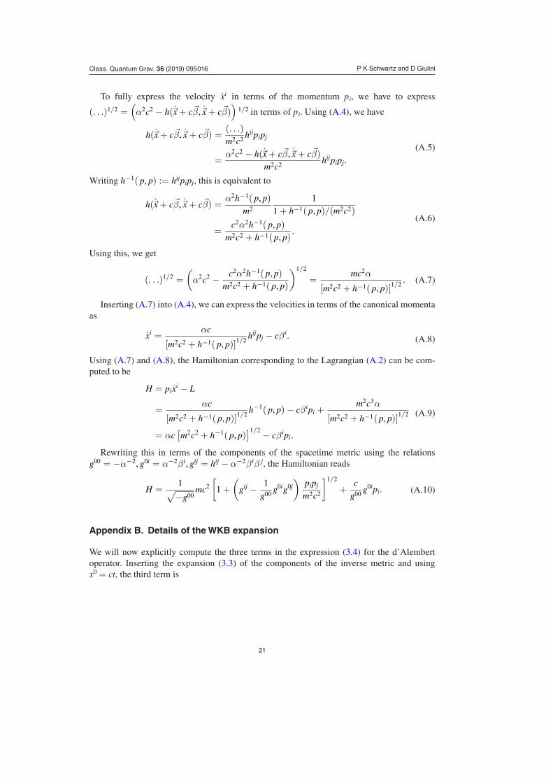
To fully express the velocity xi in terms of the momentum p i, we have to express

(. . .)1/2 =(α2c2 − h(�x + c�β,�x + c�β)

)1/2 in terms of p i. Using (A.4), we have

h(�x + c�β,�x + c�β) =(. . .)

m2c2 hijpipj

=α2c2 − h(�x + c�β,�x + c�β)

m2c2 hijpipj. (A.5)

Writing h−1( p, p) := hijpipj, this is equivalent to

h(�x + c�β,�x + c�β) =α2h−1( p, p)

m2

11 + h−1( p, p)/(m2c2)

=c2α2h−1( p, p)

m2c2 + h−1( p, p).

(A.6)

Using this, we get

(. . .)1/2 =

(α2c2 − c2α2h−1( p, p)

m2c2 + h−1( p, p)

)1/2

=mc2α

[m2c2 + h−1( p, p)]1/2 . (A.7)

Inserting (A.7) into (A.4), we can express the velocities in terms of the canonical momenta as

xi =αc

[m2c2 + h−1( p, p)]1/2 hijpj − cβi. (A.8)

Using (A.7) and (A.8), the Hamiltonian corresponding to the Lagrangian (A.2) can be com-puted to be

H = pixi − L

=αc

[m2c2 + h−1( p, p)]1/2 h−1( p, p)− cβipi +m2c3α

[m2c2 + h−1( p, p)]1/2

= αc[m2c2 + h−1( p, p)

]1/2 − cβipi.

(A.9)

Rewriting this in terms of the components of the spacetime metric using the relations g00 = −α−2, g0i = α−2βi, gij = hij − α−2βiβ j, the Hamiltonian reads

H =1√−g00

mc2[

1 +

(gij − 1

g00 g0ig0j)

pipj

m2c2

]1/2

+c

g00 g0ipi. (A.10)

Appendix B. Details of the WKB expansion

We will now explicitly compute the three terms in the expression (3.4) for the d’Alembert operator. Inserting the expansion (3.3) of the components of the inverse metric and using x0 = ct, the third term is

P K Schwartz and D Giulini Class. Quantum Grav. 36 (2019) 095016

22

gµν∂µ∂ν = −c−2∂2t +∆+

∞∑k=1

c−kg00(k)c

−2∂2t +

∞∑k=1

c−k2g0i(k)c

−1∂t∂i +

∞∑k=1

c−kgij(k)∂i∂j

= −c−2∂2t +∆+

∞∑k=3

c−kg00(k−2)∂

2t +

∞∑k=2

c−k2g0i(k−1)∂t∂i +

∞∑k=1

c−kgij(k)∂i∂j.

(B.1)

Similarly, we get

(∂µgµν)∂ν =

∞∑k=3

c−k(∂tg00(k−2))∂t +

∞∑k=2

c−k(∂tg0i(k−1))∂i

+∞∑

k=2

c−k(∂ig0i(k−1))∂t +

∞∑k=1

c−k(∂igij(k))∂j

(B.2)

for the second term.Using the form

gµν =

[(1+

∞∑k=1

c−kg−1(k)η

)η−1

]µν

(B.3)of the expanded inverse metric, we can use a formal Neumann series to invert the power series and write the coefficients of the metric as

gµν =

{η

[1+

∞∑n=1

(−

∞∑k=1

c−kg−1(k)η

)n]}

µν

. (B.4)

Iterating the Cauchy product formula, we have(−

∞∑k=1

c−kg−1(k)η

)n

= (−1)n∞∑

k=1

c−k∑

i1+···+in=k1�i1,...,in�k

g−1(i1)

η · · · g−1(in)

η. (B.5)

Using this and the notation

g−1(k,n) :=

∑i1+···+in=k1�i1,...,in�k

g−1(i1)

ηg−1(i2)

η · · · g−1(in) (B.6)

introduced in the main text, we can write the metric as

gµν = ηµν +

∞∑k=1

c−k∞∑

n=1

(−1)n(ηg−1(k,n)η)µν . (B.7)

Thus, using the Cauchy product formula again, we get

gρσ∂µgρσ =

(ηρσ +

∞∑k=1

c−k∞∑

n=1

(−1)n(ηg−1(k,n)η)ρσ

) ∞∑m=1

c−m∂µgρσ(m)

=∞∑

k=1

c−k∂µtr(ηg−1(k)) +

∞∑k=2

c−k∑

l+m=k

∞∑n=1

(−1)n(ηg−1(l,n)η)ρσ∂µgρσ(m).

(B.8)

P K Schwartz and D Giulini Class. Quantum Grav. 36 (2019) 095016

23

Using∑

l+m=k

(ηg−1(l,n)η)ρσ∂µgρσ

(m) =∑

l+m=k

∑i1+···+in=l

(ηg−1(i1)

· · · g−1(in)

η)ρσ∂µgρσ(m)

=∑

i1+···+in+m=k

tr(ηg−1(i1)

· · · g−1(in)

η∂µg−1(m))

=1

n + 1∂µ

∑i1+···+in+m=k

tr(ηg−1(i1)

· · · g−1(in)

ηg−1(m))

=1

n + 1∂µtr(ηg−1

(k,n+1)),

(B.9)

we can rewrite this as

gρσ∂µgρσ =

∞∑k=1

c−k∂µtr(ηg−1(k)) +

∞∑k=2

c−k∞∑

n=2

(−1)n−1 1n∂µtr(ηg−1

(k,n))

=

∞∑k=1

c−k∂µtr(ηg−1(k)) +

∞∑k=1

c−k∞∑

n=2

(−1)n−1 1n∂µtr(ηg−1

(k,n))

=

∞∑k=1

c−k∞∑

n=1

(−1)n−1 1n∂µtr(ηg−1

(k,n))

(B.10)

since g−1(k,n) = 0 for n > k and g−1

(k,1) = g−1(k). Thus, we finally have the expansion

1√−g

(∂µ√−g)gµν∂ν f

= −12(gρσ∂µgρσ)gµν∂ν f

=12

∞∑k=1

c−k∞∑

n=1

(−1)n 1n[∂µtr(ηg−1

(k,n))]

(ηµν +

∞∑m=1

c−mgµν(m)

)∂ν f

=12

∞∑k=1

c−k∞∑

n=1

(−1)n 1n[∂µtr(ηg−1

(k,n))]ηµν∂ν f

+12

∞∑k=2

c−k∑

l+m=k

∞∑n=1

(−1)n 1n[∂µtr(ηg−1

(l,n))]gµν(m)∂ν f

(B.11)

for the first term in the d’Alembert operator (3.4).Inserting (B.1), (B.2) and (B.11) into (3.4) and sorting the sums by order of c−1, we get the

expansion (3.7) for the d’Alembert operator.The fully expanded positive frequency Klein–Gordon equation as an equation for the func-

tion ψ in the Klein–Gordon field ΨKG = exp(imc2t/�

)ψ is as follows:

P K Schwartz and D Giulini Class. Quantum Grav. 36 (2019) 095016

24

0 =

∞∑k=5

c−k 12

∑l+m=k−2

∞∑n=1

(−1)n 1n

g00(m)[∂ttr(ηg−1

(l,n))]∂tψ

+

∞∑k=4

c−k(∂tg00(k−2))∂tψ +

∞∑k=4

c−kg00(k−2)∂

2t ψ

−∞∑

k=3

c−k im2�

∑l+m=k

∞∑n=1

(−1)n 1n

g00(m)[∂ttr(ηg−1

(l,n))]ψ

+

∞∑k=3

c−k 12

∑l+m=k−1

∞∑n=1

(−1)n 1n

g0i(m)

([∂ttr(ηg−1

(l,n))]∂iψ + [∂itr(ηg−1(l,n))]∂tψ

)

−∞∑

k=3

c−k 12

∞∑n=1

(−1)n 1n[∂ttr(ηg−1

(k−2,n))]∂tψ

−∞∑

k=2

c−k im�(∂tg00

(k))ψ −∞∑

k=2

c−k 2im�

g00(k)∂tψ

+∞∑

k=2

c−k 12

∑l+m=k

∞∑n=1

(−1)n 1n

gij(m)[∂itr(ηg−1

(l,n))]∂jψ

+

∞∑k=2

c−k((∂tg0i

(k−1))∂iψ + (∂ig0i(k−1))∂tψ

)+

∞∑k=2

c−k2g0i(k−1)∂t∂iψ − c−2∂2

t ψ

−∞∑

k=1

c−k im2�

∑l+m=k+1

∞∑n=1

(−1)n 1n

g0i(m)[∂itr(ηg−1

(l,n))]ψ

+

∞∑k=1

c−k im2�

∞∑n=1

(−1)n 1n[∂ttr(ηg−1

(k,n))]ψ

+∞∑

k=1

c−k 12

∞∑n=1

(−1)n 1n[∂itr(ηg−1

(k,n))]∂iψ +∞∑

k=1

c−k(∂igij(k))∂jψ

+∞∑

k=1

c−kgij(k)∂i∂jψ

−∞∑

k=0

c−k m2

�2 g00(k+2)ψ −

∞∑k=0

c−k im�(∂ig0i

(k+1))ψ −∞∑

k=0

c−k 2im�

g0i(k+1)∂iψ

+2im�

∂tψ +∆ψ.

(B.12)

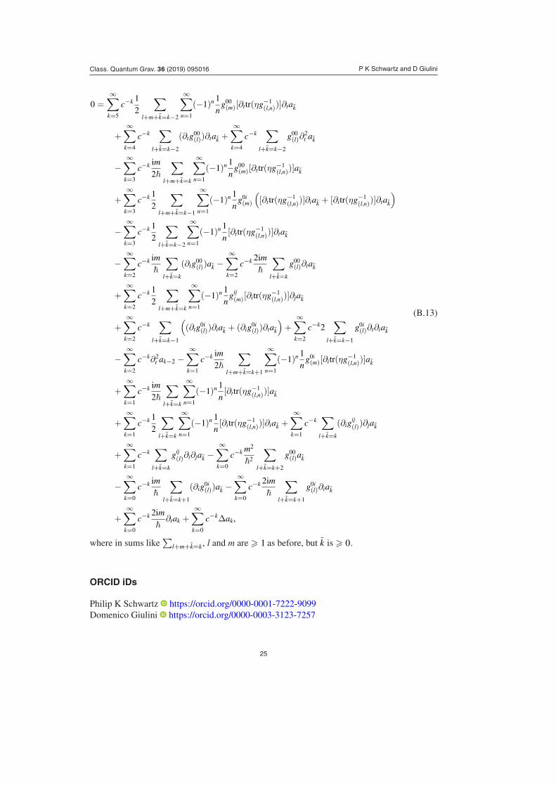
Inserting the expansion ψ =∑∞

k=0 c−kak and using the Cauchy product formula, this is equivalent to

P K Schwartz and D Giulini Class. Quantum Grav. 36 (2019) 095016

25

0 =

∞∑k=5

c−k 12

∑

l+m+k=k−2

∞∑n=1

(−1)n 1n

g00(m)[∂ttr(ηg−1

(l,n))]∂tak

+∞∑

k=4

c−k∑

l+k=k−2

(∂tg00(l))∂tak +

∞∑k=4

c−k∑

l+k=k−2

g00(l)∂

2t ak

−∞∑

k=3

c−k im2�

∑

l+m+k=k

∞∑n=1

(−1)n 1n

g00(m)[∂ttr(ηg−1

(l,n))]ak

+

∞∑k=3

c−k 12

∑

l+m+k=k−1

∞∑n=1

(−1)n 1n

g0i(m)

([∂ttr(ηg−1

(l,n))]∂iak + [∂itr(ηg−1(l,n))]∂tak

)

−∞∑

k=3

c−k 12

∑

l+k=k−2

∞∑n=1

(−1)n 1n[∂ttr(ηg−1

(l,n))]∂tak

−∞∑

k=2

c−k im�

∑

l+k=k

(∂tg00(l))ak −

∞∑k=2

c−k 2im�

∑

l+k=k

g00(l)∂tak

+

∞∑k=2

c−k 12

∑

l+m+k=k

∞∑n=1

(−1)n 1n

gij(m)[∂itr(ηg−1

(l,n))]∂jak

+∞∑

k=2

c−k∑

l+k=k−1

((∂tg0i

(l))∂iak + (∂ig0i(l))∂tak

)+

∞∑k=2

c−k2∑

l+k=k−1

g0i(l)∂t∂iak

−∞∑

k=2

c−k∂2t ak−2 −

∞∑k=1

c−k im2�

∑

l+m+k=k+1

∞∑n=1

(−1)n 1n

g0i(m)[∂itr(ηg−1

(l,n))]ak

+∞∑

k=1

c−k im2�

∑

l+k=k

∞∑n=1

(−1)n 1n[∂ttr(ηg−1

(l,n))]ak

+∞∑

k=1

c−k 12

∑

l+k=k

∞∑n=1

(−1)n 1n[∂itr(ηg−1

(l,n))]∂iak +∞∑

k=1

c−k∑

l+k=k

(∂igij(l))∂jak

+

∞∑k=1

c−k∑

l+k=k

gij(l)∂i∂jak −

∞∑k=0

c−k m2

�2

∑

l+k=k+2

g00(l)ak

−∞∑

k=0

c−k im�

∑

l+k=k+1

(∂ig0i(l))ak −

∞∑k=0

c−k 2im�

∑

l+k=k+1

g0i(l)∂iak

+

∞∑k=0

c−k 2im�

∂tak +

∞∑k=0

c−k∆ak,

(B.13)

where in sums like ∑

l+m+k=k , l and m are � 1 as before, but k is � 0.

ORCID iDs

Philip K Schwartz https://orcid.org/0000-0001-7222-9099Domenico Giulini https://orcid.org/0000-0003-3123-7257

P K Schwartz and D Giulini Class. Quantum Grav. 36 (2019) 095016

26

References

[1] Kiefer C and Singh T P 1991 Phys. Rev. D 44 1067–76 [2] Lämmerzahl C 1995 Phys. Lett. A 203 12–7 [3] Giulini D and Großardt A 2012 Class. Quantum Grav. 29 215010 [4] Wajima S, Kasai M and Futamase T 1997 Phys. Rev. D 55 1964–70 [5] Gao D F, Wang J and Zhan M S 2018 Commun. Theor. Phys. 69 37–42 [6] Pikovski I, Zych M, Costa F and Brukner Č 2015 Nat. Phys. 11 668–72 [7] Bonder Y, Okon E and Sudarsky D 2015 Phys. Rev. D 92 124050 [8] Pang B H, Chen Y and Khalili F Y 2016 Phys. Rev. Lett. 117 090401 [9] Schlippert D, Hartwig J, Albers H, Richardson L L, Schubert C, Roura A, Schleich W P, Ertmer W

and Rasel E M 2014 Phys. Rev. Lett. 112 203002[10] Zych M and Pikovski I 2018 Nat. Phys. 14 1027–31[11] Rosi G, D’Amico G, Cacciapuoti L, Sorrentino F, Prevedelli M, Zych M, Brukner Č and Tino G M

2017 Nat. Commun. 8 15529[12] Bär C and Fredenhagen K (ed) 2009 Quantum Field Theory on Curved Spacetimes (Lecture Notes

in Physics vol 786) (Berlin: Springer)[13] Wald R M 1994 Quantum Field Theory in Curved Spacetime and Black Hole Thermodynamics

(Chicago, IL: University of Chicago Press)[14] Colella R, Overhauser A W and Werner S A 1975 Phys. Rev. Lett. 34 1472–4[15] Farah T, Guerlin C, Landragin A, Bouyer P, Gaffet S, Pereira Dos Santos F and Merlet S 2014

Gyroscopy Navig. 5 266–74[16] Dimopoulos S, Graham P W, Hogan J M and Kasevich M A 2008 Phys. Rev. D 78 042003[17] İnönü E and Wigner E P 1953 Proc. Natl Acad. Sci. USA 39 510–24[18] Tagirov É A 1990 Theor. Math. Phys. 84 966–74[19] Tagirov É A 1992 Theor. Math. Phys. 90 281–8[20] Tagirov E A 1996 Theor. Math. Phys. 106 99–107[21] Tagirov E A 1999 Class. Quantum Grav. 16 2165–85[22] Tagirov E A 2003 Int. J. Theor. Phys. 42 465–97[23] Giulini D 2014 Springer Handbook of Spacetime ed A Ashtekar and V Petkov (Berlin: Springer) ch

17, pp 323–62[24] Tagirov E A 1973 Ann. Phys., NY 76 561–79[25] DeWitt B S 1952 Phys. Rev. 85 653–61[26] Sudarshan E C G and Mukunda N 2016 Classical Dynamics—a Modern Perspective (Singapore:

World Scientific)

P K Schwartz and D Giulini Class. Quantum Grav. 36 (2019) 095016