PAPER • OPEN ACCESS

Discontinuous switching of position of twocoexisting phasesTo cite this article: Samuel Krüger et al 2018 New J. Phys. 20 075009

 

View the article online for updates and enhancements.

Related contentCharge pattern matching as a ‘fuzzy’ modeof molecular recognition for the functionalphase separations of intrinsicallydisordered proteinsYi-Hsuan Lin, Jacob P Brady, Julie DForman-Kay et al.

-

Droplet ripening in concentration gradientsChristoph A Weber, Chiu Fan Lee andFrank Jülicher

-

Numerical investigation of therecrystallization kinetics by means of theKWC phase-field model with special orderparametersJulia Kundin

-

This content was downloaded from IP address 193.174.246.87 on 07/08/2018 at 19:00

New J. Phys. 20 (2018) 075009 https://doi.org/10.1088/1367-2630/aad173

PAPER

Discontinuous switching of position of two coexisting phases

Samuel Krüger1,2,3,7, ChristophAWeber1,2,4,6,7 , Jens-Uwe Sommer2,3,5 and Frank Jülicher1,2,6

1 Max Planck Institute for the Physics of Complex Systems,Nöthnitzer Str.38, D-01187Dresden, Germany2 Center for Advancing Electronics Dresden cfAED,Dresden, Germany3 Leibniz-Institut für Polymerforschung, D-01069Dresden, Germany4 Division of Engineering andApplied Sciences, HarvardUniversity, Cambridge,MA02138,United States of America5 TUDresden, Institute for Theoretical Physics, ZellescherWeg 17,Dresden, Germany6 Center for Systems BiologyDresden, CSBD,Dresden, Germany7 Equal contribution.

E-mail: julicher@pks.mpg.de

Keywords: equilibriumphase transition, liquid phase separationwith externalfield, concentration gradients, positioning, ternarymixturewith external field

AbstractLiquid–liquid phase separation leads to the formation of condensed phases that coexist with afluid.Herewe investigate how the positions of a condensed phase can be controlled by using concentrationgradients of a regulator that influences phase separation.We consider ameanfieldmodel of a ternarymixturewhere a concentration gradient of a regulator is imposed by an external potential. A novel firstorder phase transition occurs at which the position of the condensed phase switches in a discontinuousmanner. Thismechanism could have implications for the spatial organisation of biological cells andprovides a controlmechanism for droplets inmicrofluidic systems.

1. Introduction: positioning of condensed phases

Phase separation of amixture refers to the formation of a liquid condensed phase that coexists with a dilutephase of lower concentration [1, 2]. Such demixing is the result of afirst order thermodynamic phase transitionwhere the concentration difference between the phases changes discontinuously. It can be observed inmanyforms in everyday life, for examplewhen oil is added towater. The occurrence of a transition from thehomogeneousmixture to a systemwith coexisting phases can be controlled by temperature or by changing thecomposition of themixture. Condensed phases are influenced by surfaces possibly causingwetting transitions[3–5]. Furthermore, phase separation can be affected by external forces such as gravity causing sedimentation.

Akeyquestion is how liquid condensedphases such as droplets arepositioned in systemswith external cues likeconcentrationgradients or externalfields.The studyof positioningofphases provides general insights in thephysics ofphase separationof spatially inhomogeneous systems.Understanding theunderlyingmechanismof thepositioningmayopen thepossibility of applications inmicrofuidic devices. Positioned liquid condensedphases couldbeused toseal andopen junctions at specific locations in themicrofluidic device, or simplyposition chemicals that partition intothe condensedphase. Thepositioningof liquid condensedphases in a complexmixture alsoplays a role in cell biology.Inparticular, positioneddroplets areused to segregatemolecules during asymmetric cell division [6–9].

Herewe study the equilibriumphysics of the positioning of two liquid condensedphases in inhomogeneoussystems.Wepresent a simplifiedmodel that provides the basicmechanism for the positioning at thermalequilibriumwhich canbe further extended tonon-equilibriumprocesses such as the kinetics of droplet formationand ripening [10]. In ourmodel, phase separationof two components is subject to a concentration gradient of aregulator componentwhere the gradient is generated by an externalfield. The regulator component affects demixingof the two components but doesnot phase separate itself. The system then relaxes to a spatially inhomogeneousthermodynamic equilibriumstatewith two coexisting phases positionedby the regulator gradient. The spatialdistributions of the three concentrationprofiles at thermal equilibriumare determinedbyminimising ameanfieldfree energy functional.Wefind that as a functionof an interactionparameter the position of the condensedphaseswitches discontinuously fromaposition in the regionof large regulator concentration (correlated state) to the

OPEN ACCESS

RECEIVED

20December 2017

REVISED

14May 2018

ACCEPTED FOR PUBLICATION

5 July 2018

PUBLISHED

27 July 2018

Original content from thisworkmay be used underthe terms of the CreativeCommonsAttribution 3.0licence.

Any further distribution ofthis workmustmaintainattribution to theauthor(s) and the title ofthework, journal citationandDOI.

© 2018TheAuthor(s). Published by IOPPublishing Ltd on behalf ofDeutsche PhysikalischeGesellschaft

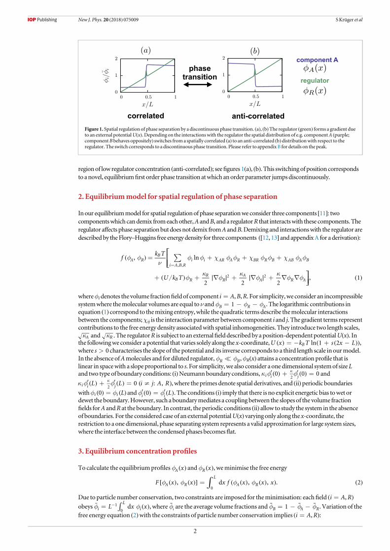
regionof low regulator concentration (anti-correlated); seefigures 1(a), (b). This switching of position correspondsto a novel, equilibriumfirst order phase transition atwhich anorder parameter jumpsdiscontinuously.

2. Equilibriummodel for spatial regulation of phase separation

Inour equilibriummodel for spatial regulationof phase separationwe consider three components [11]: twocomponentswhich candemix fromeachother,A andB, and a regulatorR that interactswith these components. Theregulator affects phase separationbut doesnot demix fromA andB.Demixing and interactionswith the regulator aredescribedby the Flory–Huggins free energy density for three components([12, 13] and appendixA for a derivation):

fk T

U k T

, ln

2 2 2, 1

A RB

i A B Ri i AR A R BR R B AB A B

B RR

RA

A R A

, ,

2 2

åf fn

f f c f f c f f c f f

fk

fk

fk

f f

= + + +

+ + + +

=

⎡⎣⎢⎢

⎤⎦⎥

( )

( ) ∣ ∣ ∣ ∣ ( )

wherefidenotes the volume fractionfieldof component i=A,B,R. For simplicity,we consider an incompressiblesystemwhere themolecular volumes are equal to ν and 1B R Af f f= - - . The logarithmic contributions inequation (1) correspond to themixing entropy,while thequadratic termsdescribe themolecular interactionsbetween the components;χij is the interactionparameter between component i and j. The gradient terms representcontributions to the free energy density associatedwith spatial inhomogeneities. They introduce two length scales,

Ak and Rk . The regulatorR is subject to an externalfielddescribed by a position-dependent potentialU(x). Inthe followingwe consider a potential that varies solely along the x-coordinate,U x k T s x Lln 1 2B= - + -( ) ( ( )),where s>0 characterises the slope of the potential and its inverse corresponds to a third length scale in ourmodel.In the absenceofAmolecules and for diluted regulator, R Bf f ,fR(x) attains a concentration profile that islinear in spacewith a slope proportional to s. For simplicity,we also consider a one dimensional systemof size Land two type of boundary conditions: (i)Neumannboundary conditions, 0 0 0i i j2

k f f¢ + ¢ =k( ) ( ) and

L L 0i i j2k f f¢ + ¢ =k( ) ( ) (i j A R: ,¹ ), where theprimesdenote spatial derivatives, and (ii)periodic boundarieswithfi (0)=fi (L) and L0i if f¢ = ¢( ) ( ). The conditions (i) imply that there is no explicit energetic bias towet ordewet the boundary.However, such a boundarymediates a coupling between the slopes of the volume fractionfields forA andR at the boundary. In contrast, theperiodic conditions (ii) allow to study the system in the absenceof boundaries. For the considered case of an external potentialU(x) varying only along the x-coordinate, therestriction to a one dimensional, phase separating system represents a valid approximation for large system sizes,where the interface between the condensed phases becomesflat.

3. Equilibrium concentration profiles

To calculate the equilibriumprofiles xAf ( ) and xRf ( ), weminimise the free energy

F x x x f x x x, d , , . 2A R

L

A R0òf f f f=[ ( ) ( )] ( ( ) ( ) ) ( )

Due to particle number conservation, two constraints are imposed for theminimisation: each field (i=A,R)obeys L x xdi

L

i1

0òf f= -¯ ( ), where if̄ are the average volume fractions and 1B A Rf f f= - -¯ ¯ ¯ . Variation of the

free energy equation (2)with the constraints of particle number conservation implies (i=A,R):

Figure 1. Spatial regulation of phase separation by a discontinuous phase transition. (a), (b)The regulator (green) forms a gradient dueto an external potentialU(x). Depending on the interactions with the regulator the spatial distribution of e.g. componentA (purple;componentB behaves oppositely) switches from a spatially correlated (a) to an anti-correlated (b)distributionwith respect to theregulator. The switch corresponds to a discontinuous phase transition. Please refer to appendix B for details on the peak.

2

New J. Phys. 20 (2018) 075009 SKrüger et al

xf

x

f f0 d

d

d, 3

L

i i

i ii

i

L

00

ò f fl df

fdf=

¶¶

-¶¶ ¢

+ +¶¶ ¢

⎛⎝⎜⎜

⎞⎠⎟⎟ ( )

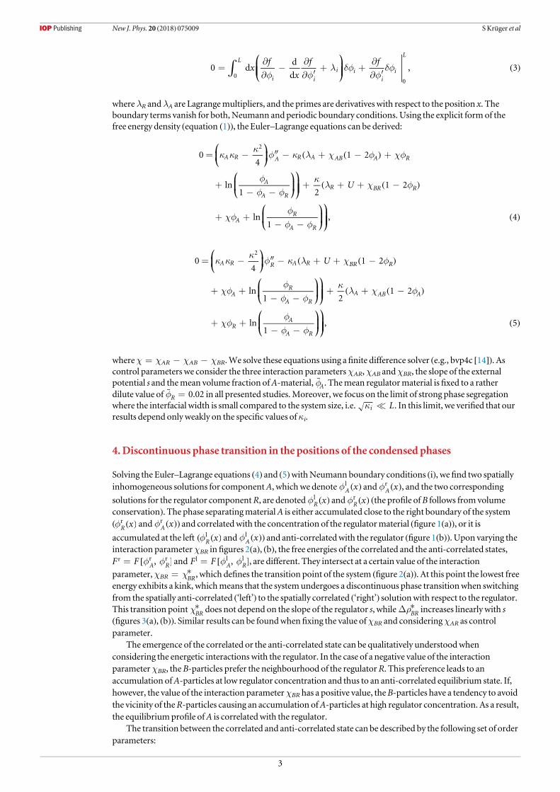
whereλR andλA are Lagrangemultipliers, and the primes are derivatives with respect to the position x. Theboundary terms vanish for both,Neumann and periodic boundary conditions. Using the explicit formof thefree energy density (equation (1)), the Euler–Lagrange equations can be derived:

U

04

1 2

ln1 2

1 2

ln1

, 4

A R A R A AB A R

A

A RR BR R

AR

A R

2

k kk

f k l c f cf

ff f

kl c f

cfff f

= - - + - +

+- -

+ + + -

+ +- -

⎛⎝⎜

⎞⎠⎟

⎛⎝⎜

⎞⎠⎟

⎞⎠⎟⎟

⎛⎝⎜

⎞⎠⎟

⎞⎠⎟⎟

( ( )

( ( )

( )

U04

1 2

ln1 2

1 2

ln1

, 5

A R R A R BR R

AR

A RA AB A

RA

A R

2

k kk

f k l c f

cfff f

kl c f

cfff f

= - - + + -

+ +- -

+ + -

+ +- -

⎛⎝⎜

⎞⎠⎟⎛⎝⎜

⎞⎠⎟

⎞⎠⎟⎟

⎛⎝⎜

⎞⎠⎟

⎞⎠⎟⎟

( ( )

( ( )

( )

whereχ=χAR−χAB−χBR.We solve these equations using afinite difference solver (e.g., bvp4c [14]). Ascontrol parameters we consider the three interaction parametersχAR,χAB andχBR, the slope of the externalpotential s and themean volume fraction ofA-material, Af̄ . Themean regulatormaterial isfixed to a ratherdilute value of 0.02Rf =¯ in all presented studies.Moreover, we focus on the limit of strong phase segregationwhere the interfacial width is small compared to the system size, i.e. Lik . In this limit, we verified that ourresults depend onlyweakly on the specific values ofκi.

4.Discontinuous phase transition in the positions of the condensed phases

Solving the Euler–Lagrange equations (4) and (5)withNeumann boundary conditions (i), wefind two spatiallyinhomogeneous solutions for componentA, whichwe denote xA

lf ( ) and xArf ( ), and the two corresponding

solutions for the regulator componentR, are denoted xRlf ( ) and xR

rf ( ) (the profile ofB follows from volumeconservation). The phase separatingmaterialA is either accumulated close to the right boundary of the system( xR

rf ( ) and xArf ( )) and correlatedwith the concentration of the regulatormaterial (figure 1(a)), or it is

accumulated at the left ( xRlf ( ) and xA

lf ( )) and anti-correlatedwith the regulator (figure 1(b)). Upon varying theinteraction parameterχBR infigures 2(a), (b), the free energies of the correlated and the anti-correlated states,F F ,A R

r r rf f= [ ]and F F ,A Rl l lf f= [ ], are different. They intersect at a certain value of the interaction

parameter,χBR= BR*c , which defines the transition point of the system (figure 2(a)). At this point the lowest free

energy exhibits a kink, whichmeans that the systemundergoes a discontinuous phase transitionwhen switchingfrom the spatially anti-correlated (‘left’) to the spatially correlated (‘right’) solutionwith respect to the regulator.This transition point BR

*c does not depend on the slope of the regulator s, while BR*rD increases linearly with s

(figures 3(a), (b)). Similar results can be foundwhen fixing the value ofχBR and consideringχAR as controlparameter.

The emergence of the correlated or the anti-correlated state can be qualitatively understoodwhenconsidering the energetic interactions with the regulator. In the case of a negative value of the interactionparameterχBR, theB-particles prefer the neighbourhood of the regulatorR. This preference leads to anaccumulation ofA-particles at low regulator concentration and thus to an anti-correlated equilibrium state. If,however, the value of the interaction parameterχBR has a positive value, theB-particles have a tendency to avoidthe vicinity of theR-particles causing an accumulation ofA-particles at high regulator concentration. As a result,the equilibriumprofile ofA is correlatedwith the regulator.

The transition between the correlated and anti-correlated state can be described by the following set of orderparameters:

3

New J. Phys. 20 (2018) 075009 SKrüger et al

k TL F x x F

x x x

d

d, ,

d , 6

ij B ijij

i j i j

ij

L

i j i j

1

1

0

ò

r nc

f f f f

f f f f

= -

= -

-

-

( ) [ ( ( ) ( )) ( ¯ ¯ )]

( ( ) ( ) ¯ ¯ ) ( )

where the squared normalisation Var Varij i j2 f f= Q Q( ) ( )with x xVar di

L

i i0

2 2òf f f= -( ) ( ( ) ¯ ), denoting the

variance and x L xi if f= Q -Q( ) ( ¯ ), whereQ(·) is theHeaviside step function. This normalisation ensures that

−1<ρij<1 andρij=±1 if x xi if f= Q( ) ( ). The derivative of the free energywith respect to the interactionparameterχij generates the covariance between the spatially dependentfieldsfi(x) andfj(x). If thefields are spatiallycorrelated,ρij>0, and if they are anti-correlated,ρij<0. Forhomogeneousfieldswith xi if f=( ) ¯ ,ρij=0.Varying the interactionparameterχBR (figure 2(b)), the order parametersρBR andρAR jumpat the transitionpoint

BR*c , while in the absence of a regulator gradient (s=0), they change smoothly (figure 2(b), grey lines). The jumpofboth order parameters in the presence of a regulator gradient indicates that the spatial correlation ofA andBwithrespect toR changes abruptly,which is expected in the case of afirst order phase transition.

Bymeans of the order parameter ρBR (equation (6))we can nowdiscuss the phase diagrams as a function ofthe interaction parameters for different volume fractions of the demixingmaterial, Af̄ .Wefind three regions(figures 4(a)–(c)): amixed region (M), where volume fraction profiles are only weakly inhomogeneous and nophase separation occurs. In addition, there are two regions, (C) and (AC), where componentsA andB phaseseparate andA is spatially correlated or anti-correlatedwith the regulatorR, respectively. There exists a triplepoint where all three states have the same free energy. For 1 2Af =¯ , the shape of the transition line betweencorrelated and anti-correlated states is straight and the transition point BR

*c is independent ofχAB (figure 4(b)).

Figure 2.Discontinuous phase transition. (a) Free energy F (equation (2)) as a function of theB–R interaction parameterχBR. Fr and Fl

are the free energies of the correlated and anti-correlated stationary solutionwith respect to the regulator gradient, respectively(figures 1(a), (b)). Lines are dashedwhen solutions aremetastable. At BR

*c , Fr and Fl intersect causing a kink corresponding to thesolution of lowest free energy. This shows that the transition between correlation and anti-correlation is a discontinuous phasetransition. The grey line depicts the behaviour of the system in the absence of an external potential. In that case, both solutions haveequal free energy andno kink is observed. (b)The order parameter ρBR (equation (6)) jumps at a certain value of the interactionparameter, BR

*c , by a value of BR*rD . The grey line shows the order parameter in the absence of an external potential. In that case, the

order parameter curves are equal for both solutions and no jump could be observed. Parameters:χAB=4,χAR=1, 0.5Af =¯ ,0.02Rf =¯ , L 7.63 10R

2 5k = ´ - , L 6.10 10A2 5k = ´ - , L 6.10 102 5k = ´ - , Ls=0.99. For plotting, ν=L/256was chosen.

Figure 3. Impact of the slope of the external potentialU(x) on the phase transition. (a)The transition point is independent on the slopeof the regulator gradient s. (b)The jumpof the order parameter at the transition point linearly increases with the slope of the gradient s.The slope of this linear dependence is influenced by Af̄ . Fixed parameters:χAB=4,χAR=1, 0.02Rf =¯ , L 7.63 10R

2 5k = ´ - ,L 6.10 10A

2 5k = ´ - , L 6.10 102 5k = ´ - , ν=L/256.

4

New J. Phys. 20 (2018) 075009 SKrüger et al

If Af̄ is decreased, the correlated state is favouredwhile for increasing Af̄ , the anti-correlated state is preferred.The transition line to themixed states is horizontal for 1 2Af =¯ (figure 4(b)). For both, larger and smaller

Af̄ -values, it becomes curved andmoves towards largerχAB interaction parameters. This behaviour can bequalitatively understood by the upshift of the demixing thresholdχAB once Af̄ deviates from1/2, as known forbinary systems. Since the regulatorR is considered to be dilute, this analogy to binary systems is a goodapproximation ( 0Rf ¯ in equation (1)). Both trends explain the parabolic shape of the positions of the triplepoint in the phase diagramswhen themean volume fraction of the demixingmaterial Af̄ is varied (figure 4(d)).

The transition line in the phase diagramsbetween the correlated and anti-correlated solution as a functionofthe interactionparameters canbe estimated analytically. In the absence of a regulator gradient (s=0), the freeenergies of both solutions are the same for all interactionparameters forwhich phase separation occurs. In thepresence of a regulator gradient, however, the free energies corresponding to the correlated and the anti-correlatedsolutions are unequal formost points in the phase diagram.The reason is that the external potentialU(x) forces theregulator to forma gradient, and thus the interactionswith the regulator lead to different free energies of thecorrelated and anti-correlated states.Only along the transition line between both states, the free energies are equal:

F F F, , 0. 7A R A Rr r l lf f f fD = - =[ ] [ ] ( )

This condition can be used to estimate the transition line for varying interaction parameters and the slope of theexternal potential s. To estimateΔFweparametrise the profiles of the stationary solutions xA

r,lf ( ) and xRr,lf ( )

using physical assumptions that are in agreementwith our numerical results. First, we idealise the alreadynarrow interface of the demixed component Af as sharp, which can be realised by a strong phase separation faraway from the critical point. Second, we use only one profile, denoted as xRf ( ), for both regulator states becausethe regulator is dilute andmaintained by the external potential. Bymeans of the numerical solution, we actuallyconfirm that x xR R

r lf f( ) ( ) close to the transition line. In addition, we approximate the regulator profile aslinear function of slopem, neglecting spatial nonlinearities that can be seen infigures 1(a), (b). In appendix Bweshow that for small enoughκR, the amount of regulator inside this peak becomenegligible. Finally, the lowvolume fractions outside the condensed phase of the demixed binaryA-B system are approximated as constantvalues outf̃ . The value of outf̃ is determined by the Flory–Huggins parameterχAB and can be calculated from thebinary phase diagramby solving ln 1 1 2AB out out outc f f f= - -(( ˜ ) ˜ ) ( ˜ ) for ABoutf c˜ ( ). The larger volume

Figure 4.Phasediagramsof our ternarymodelwith spatial regulation. (a)–(c)Phasediagram for three volume fractions 0.1, 0.5, 0.9Af =¯ { }andvarying the interactionparametersχAB andχBR. The colour codedepicts theorderparameterρBRdefined in equation (6). ComponentAis spatially correlated (C)with the regulatorprofile ifρBR<0, and anti-correlated (AC)otherwise.When the system ismixed (M),ρBR≈0,and spatial profiles of all components are onlyweakly inhomogeneous.The vertical grey line in (b) is the transition linebetweenCandACcalculatedwith the ansatz equations (8)–(10)using condition(7). The triple point (blackdot) corresponds to thepoint in thephasediagramswhere the three regionsmeet and the three free energies are equal. (d)Triple point fordifferent Af̄ values (colour code). Parameters:χAR=1,

0.02Rf =¯ , L 7.63 10R2 5k = ´ - , L 6.10 10A

2 5k = ´ - , L 6.10 102 5k = ´ - ,Ls=0.99,ν=L/256.

5

New J. Phys. 20 (2018) 075009 SKrüger et al

fraction (inside) shows aweakly linear profile (figures 1(a), (b)). For diluted regulator, the volume fraction insidethe condensed phase can bewell described as x xRin inf f f= -( ) ˜ ( ), where inf̃ is the constant volume fractioninside the condensed phase of the binaryA-Bmixture (figure 5). In summary, in the case of a diluted regulator, alinear regulator profile and strong phase separation the approximated profiles are:

x x x , 8Al

in out l outf f f f- Q - +( ) [ ( ) ˜ ] ( ) ˜ ( )

x x L x , 9Ar

in out r outf f f f- Q - + +( ) [ ( ) ˜ ] ( ) ˜ ( )

x m x L 2 . 10R Rf f- +( ) ( ) ¯ ( )

The conservation ofA determines the domain sizes of the phase separated region,

mLm

m

Lm Lm

m

2 4 2

2

8 2 4 2

2, 11

R

A R

l,rout

out out2

f f

f f f f

=- + +

+ - + - -

( )

˜ ¯

( ˜ ¯ ) ( ˜ ¯ )( )

which depends on the slope of the regulatorm. For the special case of zero slope, the domain sizes left and rightare equal, L0 0 2 1A Rl r out out f f f f= = - + -( ) ( ) ( ˜ ¯ ) ( ˜ ¯ ). To calculateΔF (equation (7)), the free energydensity (equation (1)) is integrated in the domain [0, L]. Using the approximated profiles (equations (8)–(10)),wefind

F mk T

m , 12BAR BR n

c cD -( ) ( ) ( ) ( )

where the function m( ) depends only on the parameters of the simplified solutions (see equations (8)–(10)),and reads

m L m

m L

mL

m

1

42 4 2 2

1

42 4 4

1

2

1

22 2 1

1

3. 13

R AB R l r

AB R l r

r l AB R r l

l r

2 2out

out

2 2out

2 2

3 3

f f c f

f c f

f c f

=- + + - -

- - - +

+ - + + - +

+ - ⎟

⎜⎛⎝

⎞⎠

( ) ( ¯ ( ˜ ( ) ¯ ))( )

( ˜ ( ) ¯ )( )

( ) ( ˜ ( ) ¯ )( )

( ) ( )

In the limit m 0 , the function m 0 0 = =( ) as the domain sizes of the phase separated regions becomeequal, òl(0)=òr(0), for vanishing regulator slopem. To leading order in the regulator slopem,

m m L 2 1 . 14AB Rout f c f- + -( ) ( ) ( ˜ ( ) ¯ ) ( )

The expression above indicates that for small regulator slopesm, the asymmetry of the domain sizes of the phaseseparated region òl and òr is not essential for the free energy differenceΔF. Consistently, according toequations (12) and(14), the free energy difference between the correlated and anti-correlated state vanishes(ΔF=0), if there is no regulator gradient (m=0). In the presence of a regulator gradient (m 0¹ ), the freeenergy differenceΔF is zero only ifχBR=χAR, which corresponds to the transition line BR

*c between thecorrelated and anti-correlated state according to the approximate profiles (equations (8)–(10)). This predictionis in very good agreementwith our numerical results for 1 2;Af ¯ see figures 4(b) and 6(a).

Figure 5.Comparison of approximated concentration profiles to numerically calculated profiles. (a)Anti-correlated profile and (b)correlated profile close to the correlated-anti-correlated transition line. The dashed black lines depict the simplified profiles(equations (8)–(10)) used in the analytic calculation of the free energy difference between the free energies of the two stationarysolutions,ΔF. The peak of the regulator at the interface between the condensed and dilute phase is neglected in the analytical ansatz.Fixed parameters:χAB=4,χAR=1,χBR=1, 0.02Rf =¯ , 0.5Af =¯ , L 7.63 10R

2 5k = ´ - , L 6.10 10A2 5k = ´ - , Ls=0.99,

ν=L/256.

6

New J. Phys. 20 (2018) 075009 SKrüger et al

The condition for the transition line,χAR=χBR, for the case 1 2Af ¯ (see figure 4(b)) can also beunderstood by symmetry arguments. For 1 2A Bf f ¯ ¯ and dilute regulator, switching the identity ofA andBleads to the same free energy density. Thus, in the presence of an external potential acting on the regulator, thedifference in free energy between the correlated and anti-correlated stateΔF vanishes at equal interactionparameters with respect to the regulator,χAR=χBR.

Bymeans of the approximated profiles(8)–(10) and the definition of the order parameter(6), we canestimate how the jump of the order parameter BR

*rD (definition see figure 2(b)) at the transition point dependson themodel parameters:

N G m . 15BR BR1rD -* - ( ) ( )

Wefind that the estimated BR*rD as a function of the slope of the regulator and the interaction parameterχAB

almost perfectly describes the data obtained from the numericalminimisation of the free energy (figure 6(b)).This agreement shows that the proposed stationary profiles (equations (8)–(10)) are a consistent approximationto describe the discontinuous phase transition in the case of strong phase separation and a linear and dilutedregulator profile.We could also show that the asymmetry of the phase separated domains, òl and òr, is notessential for the jumpof the order parameter (equation (14)). Instead the jump is determined by the slope of theregulator profile where the jumpheight is affected by themean amount of regulatormaterial Rf̄ and the degreeof phase separation characterised byχAB (figure 6(b)).

5.Discontinuous phase transition in a periodic domain and the presence offluctuations

Thephase diagrams (figures 4(a)–(c))dependon theboundary conditions raising the questionwhether the boundarymayplay a role for the existence of thephase transition.To this endwe considered aperiodic systemwithoutboundaries. As for thenon-periodic system,we areminimising the free energy (equation (1)), nowusingperiodicboundarieswithfi (0)=fi (L) and L0i if f¢ = ¢( ) ( ). In theperiodic domain,we alsouse a periodic external potential:

U k T Ax

Lln 1 sin 2 , 16B p w= - - -⎜ ⎟

⎛⎝⎜

⎛⎝⎜

⎛⎝

⎞⎠

⎞⎠⎟

⎞⎠⎟ ( )

whereω denotes a phase shift. The value of the phase is chosen such that the region of segregated A-material isplaced at x=0. The logarithmic formof the potential ensures that a sinus distribution of the regulator isobtained in the dilute limit.

Wefind the samemain results as for the non-periodic systemwithNeumann boundary conditions, namelythe existence of a discontinuous phase transition. In particular, wefind two stationary solutions of differentspatial correlations with respect to the regulator. They switch at BR

*c by a discontinuous phase transition(figures 7(a)–(c)). Therefore, a boundary of the system is not a necessary requirement for the emergence of thereported discontinuous phase transition since it also exists in the absence of boundaries. Thus the transition isnot induced by boundaries as for example in the case of wetting transitions [3–5].

We have also scrutinised the robustness of the phase transition in position consideringMonte Carlo studiescorresponding to themeanfield free energy density equation (1).We could confirm that the positioning

Figure 6.Phase diagram and order parameter estimated by approximated concentration profiles(8)–(10). (a)The transition betweenspatial correlation (C) and anti-correlation (AC)with respect to the regulator in theχAR–χBR-plane. Parameters:χAB=4, 0.5Af =¯ ,

0.02Rf =¯ , L 7.63 10R2 5k = ´ - , L 6.10 10A

2 5k = ´ - , L 6.10 102 5k = ´ - , Ls=0.99, ν=L/256, Lm=0.04. (b) Jumpof theorder parameter at the transition point, BR

*rD , as a function of the interaction parameterχAB for different values of Rf̄ . Additionally tothe parameters of (a),χAR=1 andχBR=1. The black line in (a) and (b) shows the result obtained fromusing equations (8)–(10); thesymbols are numerical results from theminimisation of equation (2).

7

New J. Phys. 20 (2018) 075009 SKrüger et al

mechanisms is robust against the fluctuations arising from the probabilisticMonte Carlo update and that thephase diagrams of correlated and anti-correlated states coincide qualitatively.

6. Experimental verification and outlook

The discontinuous switching of phase separation could be tested experimentally.We suggest to use a soluble saltof highmagnetic susceptibility in order to create andmaintain the regulator concentration gradient by applyingan inhomogeneousmagnetic field [15]. Phase separation in a regulator gradient could then be observed byintroducing components that phase separate in a salt dependentmanner. In particular, a pre-formed dropletcould be added to an existing regulator gradient or the regulator gradient is created after coarsening viaOstwald-ripening and coalescence is completed [10, 16–18]. The phase transition could be triggered by changing theconcentrations of the phase separatingmaterial, by changing the temperature or by adding additionalcomponents that influence the interaction parameters. The validity of our theory could be probed by comparingthe order parameter with corresponding experimentalmeasurements. In particular, the order parameter jumpat the transition point could be determined for different amounts of regulatormaterial Rf̄ (seefigure 6).

Our finding of a phase transition in the position of coexisting phases could also be relevant for applications.As the composition of condensed phases provide a distinct chemical environment (e.g. for chemical reactions),ourwork suggests a novelmechanism to control and switch chemical environments inmicrofluidic devices bythe use of a phase transition in position.

Acknowledgments

Wewould like to thankMartin Elstner andOmarAdameArana for fruitful and stimulating discussions. Thisproject was supported by theCenter for Advancing Electronics Dresden (cfAED). ChristophAWeber thanks theGermanResearch Foundation (DFG) forfinancial support. Samuel Krüger andChristophAWeber contributedequally to this work.

AppendixA. Gradient contributions in the ternary Flory–Huggins free energy density

A.1. Derivation using ameanfield approximationToderive the gradient contribution in the ternary Flory–Huggins free energy density, we start from the localmean-field free energy on the lattice and calculate the continuum limit of this free energy as shown in [19] for abinary system. The local free energy density of the three component system is derived in [20, 21] using amean-field approximation:

Figure 7.Discontinuous phase transition in a periodic potential and periodic boundary conditions. (a) Free energy F as a function oftheB–R interaction parameterχBR. F

r and Fl are the free energies of the correlated and anti-correlated stationary solutionwith respectto the regulator gradient, respectively. Lines are dashedwhen solutions aremetastable. At BR

*c , Fl and Fr intersect and the solution oflowest free energy exhibits a kink. This shows that the transition between correlation and anti-correlation is a discontinuous phasetransition. (b)The order parameter ρBR jumps at BR

*c by a value of BR*rD . Parameters:χAB=4,χAR=1, 0.1Af =¯ , 0.02Rf =¯ ,

L 7.63 10R2 5k = ´ - , L 6.10 10A

2 5k = ´ - , L 6.10 102 5k = ´ - ,A=0.5. For plotting, ν=L/256was chosen. (c)Phasediagrams of our ternarymodel for spatial regulation in a periodic potential and periodic boundary conditions ( 0.1Af =¯ ). The colourcode depicts the order parameter ρBR. ComponentA is spatially correlated (C)with the regulator profile if ρBR<0, and anti-correlated (AC) otherwise.When the system ismixed (M), ρBR≈0, and spatial profiles of all components are only weaklyinhomogeneous (no phase separation). The triple point (black dot) corresponds to the point in the phase diagramswhere the threeregionsmeet and the three free energies are equal. Parameters:χAR=1, 0.1Af =¯ , 0.02Rf =¯ , L 7.63 10R

2 5k = ´ - ,A=0.5,ν=L/256.

8

New J. Phys. 20 (2018) 075009 SKrüger et al

f k T

J

J

J

ln ln

1 ln 1

1

2, 1

, 1

, , A.1

B A A R R

A R A R

AB A A R

BR R A R

AR A R

, with

å

å

n f a f a f a f a

f a f a f a f a

a b f a f b f b

a b f a f b f ba b f a f b

= +

+ - - - -

+ - -

+ - -+

a

a b a b¹

( ) ( ( ) ( ) ( ) ( )

( ( ) ( )) ( ( ) ( )))

( ( ) ( )( ( ) ( ))

( ) ( )( ( ) ( ))( ) ( ) ( )) ( )

where ν is themolecular volume. The greek indicesα andβ indicate the positions on the lattice. Thefirst twolines describe the entropy of themixture. The remaining contributions stem from the interactions between thecomponents at neighbouring lattice sites.

In the next stepswewill perform the continuum limit. In case of the entropic contribution, we can simplyreplacefi(α)→fi(x). In order to perform the continuum limit for the energetic contributions, we rearrange thecorresponding terms as follows:

J J

J J J

1

2, 1 , 1

, , , . A.2

AB A A BR R R

AR AB BR A R

, withå a b f a f b a b f a f b

a b a b a b f a f b

- + -

+ - -a b a b¹

[ ( ) ( )( ( )) ( ) ( )( ( ))

( ( ) ( ) ( )) ( ) ( )] ( )

Each contribution can be rewritten as

J

J

, 1

1

2, 2 , A.3

AB A A

AB A A A A A2 2 2

a b f a f b

a b f a f b f a f b f a

-

= - - - +

( ) ( )( ( ))

( )[( ( ) ( )) ( ( )) ( ( )) ( )] ( )

J

J

, 1

1

2, 2 , A.4

BR R R

BR R R R R R2 2 2

a b f a f b

a b f a f b f a f b f a

-

= - - - +

( ) ( )( ( ))

( )[( ( ) ( )) ( ( )) ( ( )) ( )] ( )

J J J

J J J

, , ,

1

2, , ,

. A.5

AR AB BR A R

AR AB BR A R A R

A A R R

a b a b a b f a f b

a b a b a b f a f a f b f b

f a f b f a f b

- -

= - - +

- - -

[ ( ) ( ) ( )] ( ) ( )

[ ( ) ( ) ( )][ ( ) ( ) ( ) ( )

( ( ) ( ))( ( ) ( ))] ( )

Wecan identify the Flory–Huggins interaction parameter as J ,ij ij1

2c a b= åb ( ). In the continuum limit we can

introduce the gradient of the volume fractions as ai i if a f b f- ( ( ) ( )) , where a denotes the lattice size.We

finally obtain the free energy F x fdò= with the free energy density given as

f f xk T

x x x x2 2 2

, A.6B AA

RR A R0

2 2

nk

fk

fk

f f= + + + ⎡⎣⎢

⎤⎦⎥( ) ∣ ( )∣ ∣ ( )∣ ( ) ( ) ( )

where

f k T x x x x

x x x x

x x x x x

x x x

ln ln

1 ln 1

1

1 . A.7

B A A R R

A R A R

AR A R AB A A R

BR R A R

0 n f f f ff f f f

c f f c f f fc f f f

= ++ - - - -+ + - -+ - -

( ) ( ) ( ) ( ) ( )( ( ) ( )) ( ( ) ( ))

( ) ( ) ( )( ( ) ( ))( )( ( ) ( )) ( )

The parameters characterising the ‘penalty’ corresponding to spatial inhomogeneities areκi=a2χi B, iä{A,R},and a AR AB BR

2k c c c= - -( ).

A.2. Phenomenological derivationIn theGinzburg–Landau free energy the penalties corresponding to spatial inhomogeneities arephenomenologically introduced based on symmetry considerations:

f f2 2 2

, A.8AA

BB

RR0

2 2 2kf

kf

kf- = + +

˜ ( ) ˜ ( ) ˜ ( ) ( )

where 0ik >˜ since spatial inhomogeneities are unfavored.Moreover, f0 is the free energy density that onlydepends on the volume fractionsfi, iäA,B,R. However, only two volume fraction fields are independent dueto particle conservation and incompressibility, 1=fA+fB+fR. Thuswe canwrite∇fB=−∇fA−∇fR,leading to

f f2 2 2

. A.9AA

RR A R0

2 2kf

kf

kf f- = + + ( ) ( ) ( )

Here, A A Bk k k= +˜ ˜ , R R Bk k k= +˜ ˜ and Bk k= ˜ .

9

New J. Phys. 20 (2018) 075009 SKrüger et al

A.3. Choice of the parametersκi

In the presented studies, we have chosenκA=κ for simplicity. Please note that the derivation presented inappendix A.1 is based on ameanfield approximation and therefore it should only serve as an estimate for thevaluesκi.We chose the values for the parametersκA andκR that are consistent with these estimates (seefigurecaptions).

Appendix B. Regulator peak at the interface

The numerically obtained regulator profiles show a significant peak at the interface between theA-rich and theB-rich phase (figures 1(a), (b)). The emergence of the regulator peak can be understood by entropic andenergetic considerations of the free energy. For large and positiveχAR andχBR (corresponding to a repulsivetendencywith respect to the regulator), the energy of the systemdecreases as regulator accumulates at theinterface.Moreover, the entropy decreases as the composition of the interfacial region of all three components iscloser to awell-mixed state.

The amount of regulatormaterial that is accumulated at the interface is strongly influenced by theκi-parameters; see figure B1. Infigure B2(a), the peak area is shown for varyingκi-parameters. For simplicity, wechoseκA=κR=κ. The peak area vanishes as theκi-parameters approach zero. This behaviour is expectedsince these parameters determine the size of the interface between the phase separated phases. In this limit, theapproximated profiles (equations (8) and (10)) accurately describe the numerical solutions and thus thecorresponding predictions for the phase boundaries coincidewell with the phase boundaries obtained from thenumerical calculations.

Figure B1.Peak of regulatormaterial at the interface of the condensed phase. (a), (b)Comparison of two regulator profiles for differentvalues ofκi; (b) depicts a zoom in of (a). The graphs show that the peak area decreased as the value forκi is lowered. The decreasingpeak area is caused by a reduced peakwidthwhile the peak height remains approximately constant asκi is varied (see figures B2(a),(b)). The choice ofκi=4 is very close to set of parameters that used through the entiremanuscript. Fixed parameters:χAB=4,χAR=1, 0.02Rf =¯ , 0.5Af =¯ , s=0.99, ν=L/256.

Figure B2.Characterisation of the peak in regulator concentration. Peak area (a) and peak height (b) as a function of varyingκi valuesand different interaction parameters. The peak position is defined as the position of the largest concentration value of regulatormaterial that occurs close to the interface between the coexisting phases. The peak height refers to the regulator concentrationdifference between the peak concentration and the linearfit of the increasing regulator concentration at the position of the peak. Theintegrated difference along x is the peak area. The parametersκA,κR andκ are equal and changed simultaneously. Different values ofκhave veryminor influence on the peak height. It decreases only very little with increasingκiparameters. However, the peak areasignificantly decreases for smallerκi values. For very smallκ values, the peak area is close to zero. Fixed parameters:χAB=4,χAR=1, 0.02Rf =¯ , 0.5Af =¯ , s=0.99, ν=L/256. (c)Peak height for different Flory–Huggins parametersχAR=χBR. The peakheight shows amonotonic growth for increasingχAR=χBR. The volume fraction of the regulator at the interface increases as therepulsive tendency of the regulator with the other components ismore pronounced.We set L 7.63 10R

2 5k = ´ - ,L 6.10 10A

2 5k = ´ - , which are the same values as for the studies of the phase diagram (figures 4 and 7).

10

New J. Phys. 20 (2018) 075009 SKrüger et al

However, the peak height and thereby the existence of the peak is approximately independent ofκi(figure B2(b)). This indicates that the existence of the peakmay depend on the interaction parameters forexample. Sincewe also observed that the peak ismore pronounced at the transition line between anti-correlatedstate and correlated state, we investigated the energetic influence on the peak height along the transition line. Asderived in section 4, the transition line is governed by the conditionχAR=χBR for 0.5Af =¯ .Wefind that thepeak height increases as a function of the energetic parametersχAR=χBR (figure B2(c)). Large and positivevalues ofχAR andχBR correspond to a repulsive tendencywith respect to the regulator. This indicates that theenergetic contribution to the free energy decreases as regulator accumulates at the interface.

ORCID iDs

ChristophAWeber https://orcid.org/0000-0001-6279-0405Frank Jülicher https://orcid.org/0000-0003-4731-9185

References

[1] BrayA J 1994Theory of phase-ordering kineticsAdv. Phys. 43 357–459[2] Onuki A 2002Phase TransitionDynamics (Cambridge: CambridgeUniversity Press)[3] Cahn JW1977Critical point wetting J. Chem. Phys. 66 3667–72[4] MoldoverMandCahn JW1980An interface phase transition: complete to partial wetting Science 207 1073–5[5] PohlD andGoldburgW1982Wetting transition in lutidine-watermixturesPhys. Rev. Lett. 48 1111[6] BrangwynneCP 2011 Soft active aggregates:mechanics, dynamics and self-assembly of liquid-like intracellular protein bodies Soft

Matter 7 3052–9[7] HymanAA,WeberCA and Jülicher F 2014 Liquid–liquid phase separation in biologyAnnu. Rev. Cell Dev. Biol. 30 39–58[8] BrangwynneCP, Tompa P and PappuRV2015 Polymer physics of intracellular phase transitionsNat. Phys. 11 899–904[9] Saha S et al 2016Polar positioning of phase-separated liquid compartments in cells regulated by anmRNA competitionmechanism

Cell 166 1572–84[10] WeberCA, Lee C F and Jülicher F 2017Droplet ripening in concentration gradientsNew J. Phys. 19 053021[11] LeeCF, BrangwynneCP,Gharakhani J, HymanAA and Jülicher F 2013 Spatial organization of the cell cytoplasmby position-

dependent phase separation Phys. Rev. Lett. 111 088101[12] Flory P J 1942Thermodynamics of high polymer solutions J. Chem. Phys. 10 51–61[13] HugginsML 1942 Some properties of solutions of long-chain compounds J. Phys. Chem. 46 151–8[14] Kierzenka J and Shampine L F 2001ABVP solver based on residual control and theMATLABPSEACMTOMS 27 299–316[15] TakayasuM,Gerber R and Friedlaender F 1983Magnetic separation of submicron particles IEEETrans.Magn. 19 2112–4[16] Lifshitz IM and SlyozovVV1961The kinetics of precipitation from supersaturated solid solutions J. Phys. Chem. Solids 19 35–50[17] WagnerC 1961Theorie der Alterung vonNiederschlägen durchUmlösen (Ostwald-Reifung)Ber. Bunsenges. Phys. Chem. 65 581–91[18] Yao JH, Elder K,GuoH andGrantM1993Theory and simulation ofOstwald ripening Phys. Rev.B 47 14110[19] Safran SA 1994 Statistical thermodynmics of surface Interfaces andMembranes (Reading,MA: Addison-Wesley)[20] Sivardière J and Lajzerowicz J 1975 Spin-1 lattice gasmodel: II. Condensation and phase separation in a binary fluidPhys. Rev.A

11 2090[21] Sivardière J and Lajzerowicz J 1975 Spin-1 lattice gasmodel: III. Tricritical points in binary and ternary fluids Phys. Rev.A 11 2101

11

New J. Phys. 20 (2018) 075009 SKrüger et al