paper preprints rtn'2011 - teesside universitysst-web.tees.ac.uk/external/u0025697/rtn/rtn2011...

Paper Preprints

RTN'2011

10th International Workshop on Real-Time Networks

Porto, Portugal, July 5th 2011

In conjunction with:

23rd Euromicro International Conference on Real-Time Systems

Porto, Portugal, July 6th - 8th 2011

Editor: Michael Short Electronics & Control Group, Teesside University, UK.

10th International Workshop on Real-Time Networks Paper Preprints ________________________________________________________________________ Contents 4 Message from the chair 5 International Program Comittee 6 Workshop Program 8 Keynote Speech Abstract 10 Industry Lecture Abstract 11 On the Use of Code Mobility Mechanisms in Real-time Systems 17 Evaluating the Benefits and Feasibility of Coordinated Medium Access in MANETS 23 Time Constrained FlexRay Static Segment Scheduling 29 The Possibility of Wireless Sensor Networks for Commercial Vehicle

Load Monitoring 35 Real-time routing for low-latency 802.15.4 control networks 41 Quantifying the Channel Quality for Interference-Aware Wireless Sensor Networks 47 Existing offset assignments are near optimal for an industrial AFDX network Editor: Michael Short Copyright 2011 Politécnico do Porto. All rights reserved. The copyright of this preprint collection is with Politécnico do Porto. The copyright of the individual articles remains with their authors.

3

Message from the Chair

Welcome to Porto! It has been a pleasure to be involved with the organisation and preparation for this year’s international workshop on real-time networks, the 10th in a series which initially started as the RTLIA workshop at the 2002 ECRTS conference in Vienna. This year the workshop received 15 submissions, each of which was reviewed by at least three members of the program committee. Out of the 15 submissions, seven papers were very carefully selected for presentation at the workshop and to be included in the final proceedings, to be published in December 2011. In addition, the workshop also features a keynote speech, an industry lecture and a panel discussion session. Our aim is to closely follow previous years with an interactive format and plenty of time allocated for discussion during each of the sessions. Thanks must go to the authors and presenters for their hard work, and also to the committee members for their thoughtful and in-depth reviews. Everyone involved has contributed significantly to what promises to be a thought provoking and interesting day. Thanks are also due to all who have assisted the organisation process, including the ECRTS and RTN committee members and the CISTER-ISEP members who have helped with local arrangements. Especially worthy of praise are Gerhard Fohler, Karl-Erik Årzén, Stefan Petters, Jean-Dominique Decotignie and Luis Almeida. Finally, thanks must also go to Eduardo Tovar, and to echo his words as the 1st program chair almost a decade ago, I sincerley hope that there are many future RTN workshops! I hope that you will find this year’s workshop informative and, above all, enjoyable. Michael Short Middlesbrough, Teesside, UK.

4

International Program Comittee Luis Almeida (University of Porto, Portugal) Leandro Buss Becker (Federal University of Santa Catarina, Brazil) Gianluca Cena (Politecnico di Torino, Italy) Jean-Dominique Decotignie (Swiss Center for Microtechnology CSEM) Zdenek Hanzalek (TU Prague, Czech Republic) Sheikh Imran (University of Leicester, UK) Anis Koubaa (Al-Imam University, KSA & CISTER Research Unit, Portugal) Lucia Lo Bello (University of Catania, Italy) Pau Marti (Technical University of Catalonia, Spain) Daniel Mosse (University of Pittsburgh, USA) Luca Mottola (SICS, Sweden) Binoy Ravindran (Virginia Tech, USA) Michael Schwarz (Universitat Kassel, Germany) Michael Short (Teesside University, UK). Ye-Qiong Song (LORIA, France) Eduardo Tovar (IPP-HURRAY, Portugal) Andreas Willig (University of Canterbury, New Zealand)

5

Workshop Program Registration (08:30-09:00) Welcome (09:00-09:10) Session 1: Mobility in Real-Time Networks Chair: Zdeněk Hanzálek

Paper 1 (09:10-09:50) On the Use of Code Mobility Mechanisms in Real-time Systems Luís Lino Ferreira and Luís Nogueira (Polytechnic Institute of Porto, Portugal)

Paper 2 (09:50-10:30) Evaluating the Benefits and Feasibility of Coordinated Medium Access in MANETS Authors: Marcelo Maia Sobral and Leandro Buss Becker (Federal University of Santa Catarina, Brazil) Coffee Break (10:30-10:50) Session 2: Automotive Networks Chair: Michael Short

Paper 3 (10:50-11:30) Time Constrained FlexRay Static Segment Scheduling Authors: Zdeněk Hanzálek, David Benes and Denis Waraus (Czech Technical University in Prague, Czech Republic)

Keynote Speech (11:30-12:30) The case for Ethernet in Automotive Communications Speaker: Lucia Lo Bello (University of Catania, Italy) Lunch Break (12:30-13:30) Session 3: Wireless Sensor Networks and Applications Chair: Mário Alves

Paper 4 (13:30-14:10) The Possibility of Wireless Sensor Networks for Commercial Vehicle Load Monitoring Authors: Jieun Jung, Byunghun Song and Sooyeol Park (RFID/USN Convergence Centre, Republic of Korea / IT Convergence Research Center, Republic of Korea)

Paper 5 (14:10-14:50) Real-time routing for low-latency 802.15.4 control networks Authors: Koen Holtman and Peter van der Stok (Philips Research, Eindhoven, The Netherlands).

Paper 6 (14:50-15:30) Quantifying the Channel Quality for Interference-Aware Wireless Sensor Networks Authors: Claro Noda, Shashi Prabh, Carlo Alberto Boano, Thiemo Voigt and Mário Alves (Polytechnic Institute of Porto, Portugal / Universitat zu Lubeck, Germany / Swedish Institute of Computer Science, Kista, Sweden)

6

Workshop Program (cont.) Coffee Break (15:30-15:50) Session 4: Avionic Networks Chair: Eduardo Tovar

Paper 7 (15:50-16:30) Existing offset assignments are near optimal for an industrial AFDX network Authors: Xiaoting Li, Jean-Luc Scharbarg, Christian Fraboul and Frédéric Ridouard (Université de Toulouse, France / University of Poitiers, France).

Industry Lecture (16:30-17:30) Networking in Modern Avionics: Challenges and Opportunities Speaker: Sérgio Duarte Penna (Embraer S.A., São José dos Campos, Brazil). Session 5: Future Directions in Real-Time Network Research Chair: Jean-Dominique Decotignie (CSEM, Switzerland)

Panel Discussion (17:30-Close) Sérgio Duarte Penna (Embraer S.A., Brazil) Lucia Lo Bello (University of Catania, Italy) Christian Fraboule (Université de Toulouse, France) Hermann Kopetz (Vienna University of Technology, Austria)

7

Keynote speech: The case for Ethernet in Automotive Communications

Lucia Lo Bello

Department of Electric, Electronic and Computer Engineering University of Catania, Italy

{[email protected]} Abstract The spreading of Ethernet as an in-vehicle network for today’s cars or those in the near future is being broadly announced by spokespersons for major carmakers and automotive electronics companies. Even in the scientific community there is a growing interest in the topic, as is shown by the increasing number of studies that address the performance of Switched Ethernet or Time-Triggered Ethernet in automotive embedded systems. Several factors seem to favour the introduction of Ethernet technology in the automotive communication systems arena. Some of them are similar to those that, ten years ago, motivated the interest towards the introduction of Ethernet in automation as either a complement or replacement of traditional fieldbuses. The main motivation is the higher bandwidth provided by Ethernet (100 Mbps) as compared to current in-car networks. Such an increased bandwidth paves the way for applications, like advanced driver assistance systems, which make the volume of exchanged data in automotive communication continuously grow. Other enabling factors for using Ethernet as automotive communication network are the assessed technology and the support offered to the Internet Protocol stack (IP). The Diagnostics over Internet Protocol (DoIP) standard, currently under specification as ISO 13400, will foster the use of Ethernet as a replacement for CAN for the reprogramming (flashupdate) and in-car diagnostics of automotive Electronic Control Units (ECUs). With Internet connectivity, the IP protocol will be used in-car, opening the way to enhanced navigation functionalities, remote diagnostics and location-based services. In addition to the above mentioned features, Ethernet technology is scalable, thus meeting the scalability requirement imposed by today’s automotive systems, where the number of nodes to interconnect steadily increases. The automotive domain is however quite different from automation environments. An in-car embedded system is typically divided into several functional domains, that feature different requirements and specific constraints.In this context, the talk will discuss how and to what extent Ethernet technology is likely to step in and provide benefits to the different automotive functional domains. The potential for making Ethernet a complement or even replacement to other network technologies in their respective functional domain will be addressed. The talk will consider the TTEthernet protocol, as its design provides several appealing features for automotive communication, such as, determinism, fault-tolerance, independence of fault-containment regions, fault-tolerant global time, and legacy Ethernet integration. Recent works, in fact, addressed performance evaluation of TTEthernet. The talk will both summarise significant results from related works and present new performance results obtained in some selected case studies. Finally, some directions for further investigation into the adoption of Ethernet in cars will be given, with some reference to running projects.

8

Speaker Biography Lucia Lo Bello is Associate Professor with tenure in the Department of Computer Engineering and Telecommunications at the University of Catania. Her research interests include wireless networks and sensor networks, factory communication, distributed process control, real-time industrial embedded systems, energy-aware protocols. She received the M.D. in Electronic Engineering in 1994 and the PhD degree in Computer Engineering in 1998, both from the University of Catania. She was a visiting researcher at the Department of Computer Engineering of Seoul National University, South Korea (2000-01) with a post-doctoral position. She has served on a number of program committees of distinguished international conferences in the area of factory communication, industrial embedded systems and real-time systems, being also General Chair and Program Co-Chair of some of them. She is reviewer for several international journals. She is responsible for the University of Catania of the flexWARE Project, Flexible Wireless Automation in Real-Time Environments and the ARTISTDesign NoE on Embedded Systems Design, both projects funded by the European Commission within the 7 FP. Member of the IEC Subcommittee 65C, she actively partecipates to the standardization process. She is the recipient of the IEEE Industrial Electronics Society 2008 Early Career Award. Since 2009, she is Senior Member of the IEEE. She has published more than 120 technical papers on international conferences, books and journals in the area of wireless sensor networks, factory communication, real-time systems and distributed systems.

9

Industry Lecture: Networking in Modern Avionics - Challenges and Opportunities

Sérgio Duarte Penna

Embraer S.A., São José dos Campos, Brazil)

{[email protected]} Abstract The introduction of "Integrated Modular Avionics" (IMA) by the Radio Technical Commission for Aeronautics (RTCA DO-297) in November 2005 gave focus to new industry standards. "Avionics Full Duplex Switched Network" (ARInc 644 Part 7 "AFDX"), "Time-Triggered Protocol" (TTA Group "TTP") and "Application Executive interface" (ARInc 653 "APEX") emerged offering new levels of modularity and communality to avionic systems. These standards present new challenges for system manufacturers and integrators, but offer new opportunities to improve current analytical methods for predicting system behaviour during the design phase. This presentation provides a quick overview of these important standards and addresses challenges and opportunities arising from their adoption. Speaker Biography Sérgio Penna graduated as a Mechanical Engineer in 1978 by the Federal University of Minas Gerais in Belo Horizonte, Brazil. He joined EMBRAER in 1982 as a computer analyst working for the Flight Test Division where he is still on duty. In 2008, he obtained his Master's Degree at the National Institute of Space Research (INPE) in São José dos Campos, Brazil, in Space Engineering and Technology. He is currently responsible for a team of 5 people working at EMBRAER's Flight Test Ground Station in charge of in-house software development for flight test data post-processing systems.

10

Abstract - Applications with soft real-time requirements can

benefit from code mobility mechanisms, as long as those mechanisms support the applications’ timing and Quality of Service requirements. In this paper, a generic model for code mobility mechanisms is presented. The proposed model gives system designers the necessary tools to perform a statistical timing analysis on the execution of the mobility mechanisms that can be used to determine the impact of code mobility in distributed real-time applications.

Index Terms—Real-time systems, distributed embedded systems, mobile systems, code mobility, quality of service

I. INTRODUCTION Open real-time systems are increasingly shifting from a set

of small, local applications to powerful resource-hungry distributed applications [4]. By the very nature of open real-time systems, the availability of resources is unknown before hand and can only be reserved dynamically as new applications arrive to the system. Consequently, there is an increasing demand for supporting distributed applications with the flexibility to offload parts of their computations to neighbour or “in the cloud” nodes due to local resource scarcity. Nevertheless, the real-time behaviour of these applications must be guaranteed, both during execution and during reconfiguration, after mobility has occurred.

Therefore, open real-time systems must provide applications the support to: i) use services provided by remote components; ii) move part(s) of the application’s code to remote nodes; and ii) guarantee real-time behaviour. The first requirement can be supported by a service-based infrastructure [4], to easily and transparently interconnect local and remote parts of an application. The second requirement can be supported by code mobility frameworks which allow the installation and execution of parts of an application in remote nodes [9]. Finally, the third requirement can be supported by a real-time resource manager. Capacity reserves have been proved to be successful in improving the response times of soft real-time tasks while preserving all hard real-time constraints, both CPU [3] and network [2].

A. Related work Although not widely studied, a few solutions have already been proposed to analyse the impact of code mobility on the real-time requirements of applications.

In [11], the authors propose and experimentally characterise the behaviour of a hard real-time framework that supports the migration of tasks between nodes. However, the work does not propose a mathematical model that enables system designers to account for the impact of the mobility protocol on the overall timing behaviour of applications.

A strategy for minimising the impact of code mobility in a hierarchical preemptive fixed priority scheduling system for Real-Time Java is proposed in [10]. The authors mainly determine the points in time at which the migration process should be started, which guarantees that tasks’ deadlines are met and that the migration process is executed between consecutive evocations of a migratable task.

Statefull services require the transfer of state, whose duration depends on the length of the data being transferred. However, during this period of time no transactions can be executed on that service (blackout time). However, such determination is only possible in systems with a well-known and controlled timing behaviour. Therefore, in [12], the authors tackled the problem of minimising the blackout time by proposing a partial blocking and a non-blocking approach for state transfer.

Nevertheless, none of these works focus on the mobility mechanism itself. A mobility framework should also enable the runtime relocation of services in response to reconfiguration/update events (e.g., the system might reconfigure itself due to the disappearance of a node involved in a computation). As an example, consider running a video game on a mobile device that offloads parts of its computations to neighbour nodes. Reconfiguration in such a cooperative execution might be required if one of the nodes, currently running one of game’s services, is no longer capable of outputting the required QoS. In such case, the service should be migrated to another node. Ideally, such change should be executed seamlessly, i.e. the game delays should (preferably) be unnoticeable. Examples of works that tackle

On the Use of Code Mobility Mechanisms in Real-time Systems

Luís Lino Ferreira, Luís Nogueira {llf, lmn}@isep.ipp.pt

CISTER/ISEP - Polytechnic Institute of Porto Porto, Portugal

11

the specific problems stated above are [4] and [1]. The former allows the determination of a distributed configuration that maximises the satisfaction of the user’s QoS preferences among a set of allowed QoS levels. The latter tries to fulfil the same goals, but each service is only allowed to specify a single QoS level.

B. Contribution and paper structure Service mobility in a distributed execution environment is a

complex operation that evolves through several phases, including sending the code and state to the destination node and rebinding connections between services. Additionally, resources must be explicitly reserved on the destination node, prior to the start of the mobility process. Due to its complexity, we propose that a Mobility Management framework (represented in Figure 1 by Mx) should control mobility of services between nodes of a distributed system. This paper focuses on the model and timing analysis for a generic code mobility mechanism for distributed soft real-time applications. The proposed model is generic enough, helping the system designer to define the most appropriate parameters for the mobility management modules and to determine the feasibility of the timing constrains imposed on applications, including mobility/reconfiguration events.

The remainder of the paper is organised as follows. Section II defines the generic model for the distributed applications and for the mobility mechanism. Section III discusses and analyses the code mobility phases and their timings. The main consequence of the mobility mechanism is the introduction of a bounded inaccessibility period during which the service being moved is not available. The proposed analysis allows computing the adequate resources required by the mobility framework to guarantee the timeliness of the application. Finally, Section IV discusses the model provided in the paper and presents some conclusions.

II. SYSTEM MODEL

A. Module components This work applies to soft real-time applications composed

by a set of interconnected services, each supplying some service, either in the same local node, but particularly when services are distributed among several nodes. The model considers the system to be composed of a set of N nodes {H1, ..., HN} and a set of M services {S1, …, SM}. Services are interconnected through links. lx,y characterises a connection between services Sx and Sy, (Figure 1). Each service and each link has a set of real-time requirements that are out of the scope of this paper (a detailed discussion can be found in [4]).

Each node runs a Mobility Management module Mx, where x is the index of the node. Each module Mx can be connected to other Mobility Management modules My through a network connection, lmx,my.

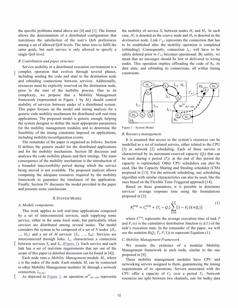
As depicted in Figure 1, an operation mS5H3→H4 represents

the mobility of service S5 between nodes H3 and H4. In such case, H3 is denoted as the source node and H4 is denoted as the destination node. Link l’6,5 represents the connection that has to be established after the mobility operation is completed (rebinding). Consequently, connection l6,5 will have to be safely deleted prior to l’6,5 becomes operational. By safely, we mean that no messages should be lost or delivered to wrong nodes. This operation implies offloading the code of S5, its data state, and rebinding its connections, all within timing constraints.

Figure 1 – System Model

B. Resource management It is assumed that access to the system’s resources can be

modelled as a set of isolated servers, either related to the CPU [3] or network [2] scheduling. Each of these servers is characterised by its maximum reserved capacity (Qi) that can be used during a period (Ti); at the end of this period the capacity is replenished. Other CPU schedulers can also be used, like the Capacity Sharing and Stealing scheduler (CSS) proposed in [13]. For the network scheduling, any scheduling algorithm with similar characteristics can also be used, like the ones based on the Flexible Time-Triggered approach [14].

Based on these guarantees, it is possible to determine services’ average response time using the formulations proposed in [3]:

��

��

�

��

��

��

(1)

where Cavgi represents the average execution time of task T

and FC(x) is the cumulative distribution function (c.d.f.) of the task’s execution time. In the remainder of the paper, we will use the notation R(Qi, Ti, FC

i()) to represent Equation (1).

C. Mobility Management Framework We assume the existence of a modular Mobility

Management framework in each node, similar to the one proposed in [9].

These mobility management modules have CPU and networking servers assigned to them, guaranteeing the timing requirements of its operations. Servers associated with the CPU offer a capacity of CF over a period TF. Network resources are split between two channels, one for bulky data

S1

S2

S3 S4

S6

S5

S'5

H2 H3

H1Hl1,6

mS5 H3→H4

l6,5

l1,2

l2,3 l2,4

l6,1

l’6,5

M1 M4

M2 M3

S'H4

12

transfer and another for the exchange of short control messages. The first has a capacity of Bdata and a period of Tdata while the second has a capacity of Bctrl and a period of Tctrl. The main advantage of using these two channels is that we can guarantee small response time for control messages, but for larger data transfer we are able to make the transfer with small overhead.

D. Service’s internal state In the proposed model, services are able to split their

internal state into different State Items, representing different variables, different objects or combinations of both. It is up to the service to define how state items are configured. The state of a service is thus a set of state items defined exclusively by the service, where a State Item (SISi

p) is only associated to a service Si and defined as a tuple:

��

��

�� IDSi

p univocally identifies this State Item and BSip is the

bandwidth required for the transfer of this state item. Some state items are created during the service initialisation and are not changed subsequently, while others are updated regularly when service calls are executed. Therefore, state items are divided in two groups: one that can be migrated during the normal operation of the service (Static Sate Items) and another that can only be migrated if there are no ongoing service calls (Dynamic State Items).

Based on the model exposed in this section, Section III shows how it is possible to devise a timing model for a generic mobility mechanism.

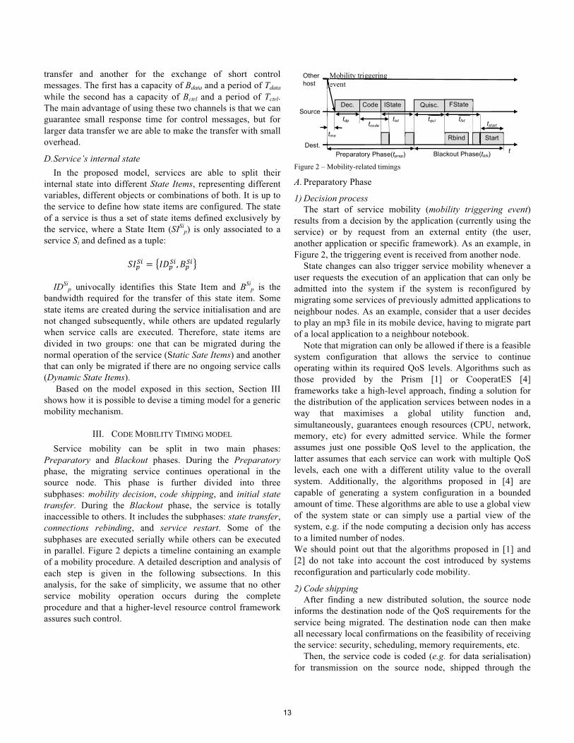
III. CODE MOBILITY TIMING MODEL Service mobility can be split in two main phases:

Preparatory and Blackout phases. During the Preparatory phase, the migrating service continues operational in the source node. This phase is further divided into three subphases: mobility decision, code shipping, and initial state transfer. During the Blackout phase, the service is totally inaccessible to others. It includes the subphases: state transfer, connections rebinding, and service restart. Some of the subphases are executed serially while others can be executed in parallel. Figure 2 depicts a timeline containing an example of a mobility procedure. A detailed description and analysis of each step is given in the following subsections. In this analysis, for the sake of simplicity, we assume that no other service mobility operation occurs during the complete procedure and that a higher-level resource control framework assures such control.

Figure 2 – Mobility-related timings

A. Preparatory Phase

1) Decision process The start of service mobility (mobility triggering event)

results from a decision by the application (currently using the service) or by request from an external entity (the user, another application or specific framework). As an example, in Figure 2, the triggering event is received from another node.

State changes can also trigger service mobility whenever a user requests the execution of an application that can only be admitted into the system if the system is reconfigured by migrating some services of previously admitted applications to neighbour nodes. As an example, consider that a user decides to play an mp3 file in its mobile device, having to migrate part of a local application to a neighbour notebook.

Note that migration can only be allowed if there is a feasible system configuration that allows the service to continue operating within its required QoS levels. Algorithms such as those provided by the Prism [1] or CooperatES [4] frameworks take a high-level approach, finding a solution for the distribution of the application services between nodes in a way that maximises a global utility function and, simultaneously, guarantees enough resources (CPU, network, memory, etc) for every admitted service. While the former assumes just one possible QoS level to the application, the latter assumes that each service can work with multiple QoS levels, each one with a different utility value to the overall system. Additionally, the algorithms proposed in [4] are capable of generating a system configuration in a bounded amount of time. These algorithms are able to use a global view of the system state or can simply use a partial view of the system, e.g. if the node computing a decision only has access to a limited number of nodes. We should point out that the algorithms proposed in [1] and [2] do not take into account the cost introduced by systems reconfiguration and particularly code mobility.

2) Code shipping After finding a new distributed solution, the source node

informs the destination node of the QoS requirements for the service being migrated. The destination node can then make all necessary local confirmations on the feasibility of receiving the service: security, scheduling, memory requirements, etc.

Then, the service code is coded (e.g. for data serialisation) for transmission on the source node, shipped through the

tdp

Preparatory Phase(tprep)

Dec. IState

tist tcode

Mobility triggering event

Code Quisc. FState

tqui tfst

Rbind

tstart

Start

Blackout Phase(tblk) t

tme

Dest.

MeMe

Other host

Source

13

network, and decoded on the destination node (e.g. by using a deserialisation method).

The bandwidth required to transfer the code is equal to βcode, a constant, since the code size is not expected to vary during transit. Therefore, the average time required for the transmission of code (tcode) can be calculated by:

FCcode,S() and FC

code,D() are the c.d.f. of the execution time required by the framework, on the source and destination nodes, respectively.

3) Initial state transfer We assume that a set of Static State Items (e.g.

configuration data) can be transferred prior to the quiescence of the service on the source node. After the transfer of the state items, the destination node acknowledges its reception. Consequently, the delay associated with the initial state transfer is given by:

��

��

��

��

� � ��

��

��

(3)

where FCist,N() is the c.d.f. for the required bandwidth, FC

ist,S() and FC

ist,D() are the c.d.f. of the CPU processing time, on the source and destination node, respectively.

4) Total delay of the Preparatory phase The time required for the Preparatory phase is given by:

��

��

�� (4)

where tme is the time that elapses from the event that triggered the mobility of a service until being received by the node responsible to determine a new system configuration. It is assumed that the new system configuration is computed in a bounded time tdp [4].

It is important to note that, depending on the scenario, some of these timings can be equal to zero. As an example, assume the case where it is the user that decides to migrate its application from its mobile device to its TV, then tme is equal to zero..

Most importantly, during this phase the service continues totally operational, but the characterisation of this delay is required in order to determine the dynamics of the mobility procedure.

B. Blackout Phase

1) Quiescence achieving Usually, in reconfiguration operations, the service to be

updated has to be in a safe state called quiescence [7]. In this state, the service being migrated: i) is not currently engaged in a transaction; ii) will not initiate a new transaction; iii) is not servicing a transaction; and iv) no transaction has or will be

initiated by other services that require service from this service. At the same time, all services connected with the migrating service must go into a passive state, which requires the fulfilling of condition i) and ii).

One initial solution to achieve quiescence has been proposed in [7], while a less demanding solution, called tranquillity was later proposed in [8]. Achieving quiescence requires the completion of pending requests by the service being migrated and the knowledge of all other services that might issue new requests. These other services must evolve into a passive state in which they cannot evoke the service being migrated, although they can evoke other services available in the system. The time needed to achieve quiescence can be determined through a timing analysis of the mechanisms proposed in [7] or [8]. This calculation, out of the scope of this paper, is assumed to be known and equal to tq.

We argue that achieving quiescence is not a necessary condition for the mobility of services in a distributed system, as shown by the implementation described in [9], if the service calls are stored by the mobility management and delivered to the destination node only after the completion of the mobility procedure.

2) Final state transfer Several different approaches can be considered for state

transfer: i) transfer all state in a single bundle [10]; ii) propagate only the operations done on state items [5]; iii) separate the state space into several groups of items, each transferred with its own periodicity [6] or iv) retransmit the state whenever it changes [12]. The mobility model here considered adapts to these approaches.

The final state transfer is the subphase that mostly influences the latencies of a service migration, due to its duration and due to the service being in a quiescent state (it involves the transfer of Dynamic State Items which can only maintain consistency if the service is not operational).

The set of state items that can only be transferred after achieving quiescence require a bandwidth of FC

fst,N() and CPU processing requirements of FC

fst,S() and FCfst,D(), respectively

on the source and destination nodes. CPU processing is required for the preparation of the data to

be sent and the required processing time to decode the data on the destination node. Therefore, the final state transfer duration (tfst) can be calculated, similarly to the case of tist, as follows:

��

��

�

��

��

� � ��

��

�

��

(5)

3) Connections rebinding In the migration process, connections between services need

to be changed according to the new location of the migrating service.

��

��

��

� � ��

��

�� (2)

14

This procedure can be performed in parallel with the final state transfer and it involves the exchange of messages between 2 or more nodes: the source, destination and, if any, other nodes whose services connect to the service being migrated. It mainly requires the exchange of messages containing the location of the new end points, which requires a bandwidth of βSi

reb. Therefore, if service Si has nconSi connections with other nodes, the total bandwidth required to rebind all connections (βreb) is nconSi×βSi

reb. The time required internally by each service to change the connection end point addresses is considered negligible.

The exchanged messages can also be used to withdraw all connected services from the passive state. Therefore, the rebinding time (trbind) is given by:

�� (6)

Since the number of exchanged message can be high, but with a small payload, its transmission is performed by the communication server assigned for control messages.

4) Service restart The final subphase, which starts at the end of both the

connection rebinding and final state transfer subphases, is responsible for the restart of the service on the destination node. All code and state must already be on the destination node and all necessary operations for the installation of the service (if required) have been completed. After being started, the service re-establishes its internal state using the state items previously transferred and enters full operation. This operation is performed by the service using its scheduling budget (CD

Si, TD

Si), and therefore the time required for service restart is given by:

��

��

�� (7)

where FCfst,D() is the p.d.f. of the CPU requirements for service

restart on the destination node.

5) Total delay of the Blackout phase During this phase, all transactions involving the migrating

service are stopped, thus leading to a blackout period (tblk). On a real-time system this time is particularly important since it influences the timeliness of the distributed application. Therefore, the total duration of the Blackout phase is given by:

�� (8)

Since the final state transfer and the rebinding of connections can be executed in parallel, then we use the function �� to determine the maximum of both subphases.

As discussed previously, the Quiescence Achieving subphase might be eliminated if the system is supported by adequate mobility management facilities. The rebinding process is based on a simple exchange of messages and on the reconfiguration of transmission and receptions ports. The

service restart is an operation with a small overhead. But, the final transfer subphase delay varies with the size of the data being transferred. Particularly, when the state size is high, strategies like the ones proposed in [12] can be used in order to reduce tfst. Such strategies enable the implementation of partial blocking and non-blocking approach on service calls for a migrating service.

IV. MOBILITY FRAMEWORK ARCHITECTURE AND IMPLEMENTATION

A Mobility Framework, which enables the mobility of services on the Android Operating system, has been developed. The framework will be used to demonstrate the use of the proposed model on real scenarios.

The framework is implemented as an Android service, which takes care of service migration, to and from another node, at the same time it interacts with the operating system Resource Manager in order to determine if the QoS requirements of the service can be supported.

The Android operating system is used both due to its open source nature to its innovative architecture. Although its use to support real-time applications is still debatable [15] it nevertheless provides a suitable architecture for quality of service-aware applications in ubiquitous, embedded systems [16].

The core services provided by the framework are the: Discovery Manager, Package Manager, State Manager and Execution Manager. Additionally, the framework also relies on a QoS Manager module that is responsible for assuring that QoS requirements of each service can be met.

The Discovery Manager module is designed to discover neighbour devices on a local network and advertise the host device capabilities. The advertise messages contain information about the applications and services installed, their associated intents interfaces and QoS requirements. Originally, Android intents provide the means for the reutilization of functionalities implemented by other application installed in the same device. Therefore, the Discovery Manager provides a standard mechanism, for each node, to obtain information about installed services and about the availability of resources in neighbour devices. It also keeps track of node and service disconnections from the network.

The Package Manager is used to install, uninstall and transfer the code of Android services, which are contained in APKs files. This module is also responsible for the interaction with the QoS Manager in order to request specific QoS levels for the service being handled. Therefore, its is the responsibility of the QoS Manager to accept or reject service installations, particularly if the QoS required level cannot be guaranteed.

The State Manager handles both the initial and final state transfer operations in a flexible way, based on the state items paradigm.

15

The Execution Manager allows launching services on a host device or on a remote node through the exchange of Android intents that allow the programming of transparent applications (in relation to the distribution). In this implementation an intent resolution procedure, based on the data collected by the Discovery Manager, determines if the intent can be run locally or if it must be redirected to the node, where the service is running.

The QoS Manager administers the system resources, either locally, on a node, or in a distributed environment. It also encapsulates the functionalities of high level QoS control frameworks, like the one defined in [4]. Consequently, this module can interact with our framework conveying orders for the deployment of services in the distributed system.

V. CONCLUSIONS AND FUTURE WORK This paper proposed a generic model for code mobility in

soft real-time systems, where applications are constituted by interconnected distributed services.

The main consequence of mobility to the running application is that it might result on a temporary degradation on the provided quality of service, due to the consequent blackout period. We state that it is up to the application programmer to determine the amount of degradation that can be supported by the application. As such, this work gives the system designer the necessary tools to perform a statistical timing analysis on the execution of the mobility mechanisms and to determine the most appropriate parameters of the mobility framework modules, either in relation to the local (CPU) or to network resources.

The proposed model divides the mobility mechanism in two phases, thus allowing a reduction on the time during which a service is inaccessible (the Preparatory phase is not considered). This work can leverage future research in the field of code mobility and service update in distributed real-time systems. The proposed analysis can support the development and evaluation of suitable mobility mechanisms. Future work will focus on the use of the state items paradigm to propose new state transfer algorithms.

ACKNOWLEDGEMENTS This work was supported by the ENCOURAGE project,

funded by National Funds through the FCT - Portuguese Foundation for Science and Technology, as well as by the ARTEMIS Joint Undertaking, under grant agreement n° 269354.

REFERENCES [1] S. Malek, G. Edwards, Y. Brun, H. Tajalli, J. Garcia, I. Krka, N.

Medvidovic, M. Mikic-Rakic, G. Sukhatme, "An Architecture-Driven Software Mobility Framework," Journal of Systems and Software, Vol. 83 Issue 6, June, 2010, pp 972-989.

[2] T. Nolte and K. Lin, “Distributed Real-time System Design using CBS-based End-to-end Scheduling,” in Proc. of the 9th International conference on Parallel and Distributed Systems, pp. 355 – 360, 2002.

[3] L. Abeni, G. Buttazzo, “Integrating multimedia applications in hard realtime systems”, in Proceedings of the 19th IEEE Real-Time Systems Symposium, Madrid, Spain, 1998, p. 4.

[4] L. Nogueira and L. Pinho, "Time-bounded Distributed QoS-Aware Service Configuration in Heterogeneous Cooperative Environments", in Journal of Parallel and Distributed Computing, Vol. 69, Issue 6, June 2009, pp. 491-507.

[5] D. Bourges-Waldegg, Y. Duponchel, M. Graf and M. Moser, "The fluid computing middleware: bringing application fluidity to the mobile Internet", in Proc. of the 2005 Symposium on Applications and the Internet, pp. 54- 63, 2005.

[6] D. Preuveneers and Y. Berbers, “Context-driven migration and diffusion of pervasive services on the OSGi framework”, in International Journal of Autonomous and Adaptive Communications Systems, Vol. 3, No. 1, pp. 33-22, 2010.

[7] J. Kramer and J. Magee, “The Evolving Philosophers Problem: Dynamic Change Management”, in IEEE Trans. on Software Engineering, Vol. 16, Issue 11 (Nov. 1990), pp. 1293-1306.

[8] Y. Vandewoude, P. Ebraert, Y. Berbers and T. D'Hondt, “An alternative to Quiescence: Tranquility”, in Proc. of the 22nd IEEE Int. Conf. on Software Maintenance, Washington, DC, (Sep. , 2006), pp. 73-82.

[9] J. Gonçalves, L. Ferreira, L. Pinho and G. Silva, “Handling Mobility on a QoS-Aware Service-based Framework for Mobile Systems”, in Proc. of the 8th IEEE International Conference on Embedded and Ubiquitous Computing (EUC 2010), Hong Kong, December 2010, to be published.

[10] M. ALRahmawy, A. Wellings, “A model for real time mobility based on the RTSJ,” in Proc. of the 5th international Workshop on Java Technologies For Real-Time and Embedded Systems (Vienna, Austria, Sep. 2007), vol. 231. ACM, New York, NY, pp. 155-164.

[11] B. K. Choi, S. Rho, R. Bettati, "Fast software component migration for applications survivability in distributed real-time systems," in Proc. of the 7th Object-Oriented Real-Time Distributed Computing, Vienna, Austria, May 2004, pp.269-276.

[12] S. Rho, R. Bettati, "Fast software component migration for applications survivability in distributed real-time systems," in Proc. of the 7th Object-Oriented Real-Time Distributed Computing, Vienna, Austria, May 2004, pp.269-276.

[13] E. Schneider, “A Middleware Approach for Dynamic Real-Time Software Reconfiguration on Distributed Embedded Systems”, PhD Thesis, Université Louis Pasteur – Strasbourg, 2004.

[14] Nogueira, L., Pinho, L., "A Capacity Sharing and Stealing Strategy for Open Real-time Systems", Published in Journal of Systems Architecture, Volume 56, Issues 4-6, April-June 2010, pp. 163-179.

[15] P. Pedreiras, P. Gai, L. Almeida, G. Buttazzo, “FTT-ethernet: A flexible real-time communication protocol that supports dynamic QoS management on ethernet-based systems”, IEEE Transactions on Industrial Informatics, vol. 1, no. 3, p. 162-172, August 2005.

[16] Maia, C., Nogueira, L., Pinho, L., “Evaluating Android OS for Embedded Real-Time Systems”, Proceedings of the 6th International Workshop on Operating Systems Platforms for Embedded Real-Time Applications (OSPERT 2010), Brussels, Belgium, 2010, pp. 63-70.

Maia, C., Noqueira, L, Pinho, L., “Cooperative embedded application in Android Environments”, Submitted for publication on the 8th International Workshop on Java Technologies for Real-time and Embedded Systems - JTRES 2010.

16

Evaluating the Benefits and Feasibility ofCoordinated Medium Access in MANETS

Marcelo Maia SobralDept of Automation and Systems

Federal University of Santa CatarinaFlorianopolis, SC - BrazilEmail: [email protected]

Leandro Buss BeckerDept of Automation and Systems

Federal University of Santa CatarinaFlorianopolis, SC - Brazil

Email: [email protected]

Abstract—A mobile ad-hoc wireless network is characterizedby a highly-dynamic topology where neither the duration oflinks between nodes nor their density within the network canbe predicted. To better understand the effect of such issues inthe medium access we provide a performance evaluation of twodistinct MAC protocols. The first is our previously proposed HCT(Hybrid Contention/TDMA) Real-Time MAC protocol, whichcontinuously adapts to topology modifications to provide a kind ofcoordinated medium access. Its performance is compared with acontention-based, non-coordinated CSMA protocol. We compareboth protocols with respect to their ability to deliver messagesin a timely manner in special simulated networks scenarios thatdeal with mobile nodes. More specifically, we compare both theratio of messages delivered within their deadlines and mediumutilization presented by these protocols in networks with differentspatial densities and speeds of nodes. Our study also analyzesthe feasibility of using such adaptive protocol in respect to itsoverhead.

I. INTRODUCTION

Analyzing some new-generation embedded applications onecan see that they rely on mobile-connectivity. For instance, inthe CarTel project [1] data is collected from sensors locatedon automobiles that move around the city. Modern IntelligentTransportation Systems use vehicle-to-vehicle (V2V) systemslike platooning, which helps to reduce traffic congestions andprovide safe driving [2]. The space community is developingdistributed satellite systems (DSS) [3], where multiple mini-satellites in varying configurations are used to achieve amission’s goals collaboratively. Most of these applicationsrequire some kind of QoS guarantee in respect to the timelydelivery of messages.

It happens that mobility causes topology changes and tem-porary link disruptions, affecting communications predictabil-ity. So the challenge in this context is how to rely on wirelesslinks to achieve timing guarantees. This issue presents a kindof contradiction in the real-time domain, as it conflicts withthe need for temporal determinism.

Several existing MAC protocols where designed to handlesuch mobility issues. In [4], Kumar et al presented a surveyabout MAC protocols used in ad-hoc wireless networks. Thewell known Z-MAC [5], for instance, is a dynamic protocolthat adapts itself to the network conditions, using CSMAduring normal workload and TDMA in high workload. Itsdrawback comes from the high overhead for reconfigurations

(about 30s according to authors), which makes it not suitablefor mobile applications. Another example is the AdHoc-MAC[6], which was conceived for inter-vehicles communicationusing a distributed TDMA slot allocation mechanism namedRR-ALOHA. Its drawback comes from the need of configuringthe application offline, making it not applicable for mobileapplications.

Despite the limitations of such protocols, it is concludedthat hybrid approaches to medium access are the key toachieve timely behavior in mobile networks. Inspired on thatwe proposed the so-called Hybrid Contention/TDMA-based(HCT) MAC [7], which aims to provide a time boundedmedium access control for mobile nodes that communicatethrough an ad-hoc wireless network. The key issue in thisprotocol is to self-organize the network in groups of adjacentnodes called clusters, as a mean to solve the problem of timelytransmission of messages. It assumes a periodic messagemodel and a transmission cycle divided in time-slots, whereeach cluster reserves a predefined number of time-slots thatcan be assigned to its member nodes.

A. Goals and Structure of the Paper

The current paper presents and discusses results obtainedfrom an intensive simulation study related to mobile appli-cations that rely on timely delivery of messages. Its goalis to emphasize the benefits of having coordinated mediumaccess to achieve the timing requirements when compared toa contention-based approach (CSMA). We also present somehints on the existing performance bounds of the protocols.To conclude, our study analyzes the feasibility of using anadaptive protocol like HCT-MAC in respect to its overhead.

In the simulations we compare both the ratio of messagesdelivered within their deadlines and the medium utilizationpresented by HCT-MAC and CSMA protocols in networkswith different spatial densities and speeds of nodes.

The remainder of the paper is structured as follows: sectionII provides an overview of our HCT-MAC protocol. SectionIII details the performance parameters to be analyzed in ourcomparison. Section IV presents the simulation experimentsperformed and discusses the obtained results. Section V con-cludes the paper.

17

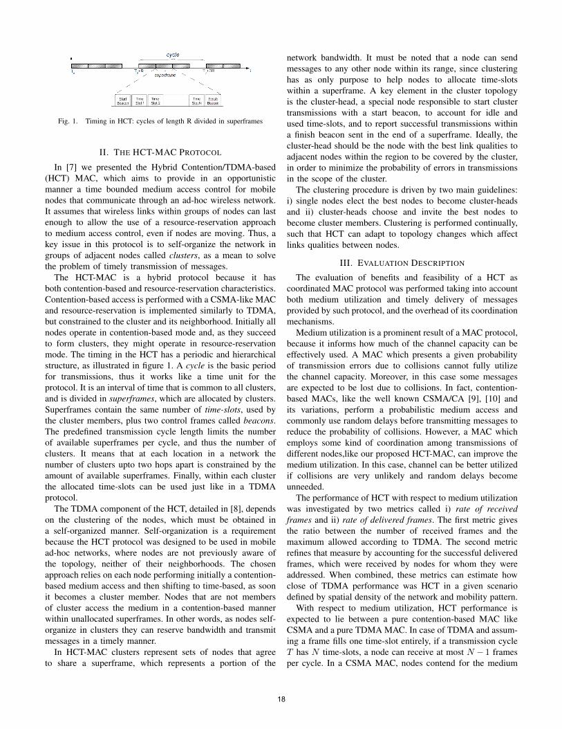
Fig. 1. Timing in HCT: cycles of length R divided in superframes

II. THE HCT-MAC PROTOCOL

In [7] we presented the Hybrid Contention/TDMA-based(HCT) MAC, which aims to provide in an opportunisticmanner a time bounded medium access control for mobilenodes that communicate through an ad-hoc wireless network.It assumes that wireless links within groups of nodes can lastenough to allow the use of a resource-reservation approachto medium access control, even if nodes are moving. Thus, akey issue in this protocol is to self-organize the network ingroups of adjacent nodes called clusters, as a mean to solvethe problem of timely transmission of messages.

The HCT-MAC is a hybrid protocol because it hasboth contention-based and resource-reservation characteristics.Contention-based access is performed with a CSMA-like MACand resource-reservation is implemented similarly to TDMA,but constrained to the cluster and its neighborhood. Initially allnodes operate in contention-based mode and, as they succeedto form clusters, they might operate in resource-reservationmode. The timing in the HCT has a periodic and hierarchicalstructure, as illustrated in figure 1. A cycle is the basic periodfor transmissions, thus it works like a time unit for theprotocol. It is an interval of time that is common to all clusters,and is divided in superframes, which are allocated by clusters.Superframes contain the same number of time-slots, used bythe cluster members, plus two control frames called beacons.The predefined transmission cycle length limits the numberof available superframes per cycle, and thus the number ofclusters. It means that at each location in a network thenumber of clusters upto two hops apart is constrained by theamount of available superframes. Finally, within each clusterthe allocated time-slots can be used just like in a TDMAprotocol.

The TDMA component of the HCT, detailed in [8], dependson the clustering of the nodes, which must be obtained ina self-organized manner. Self-organization is a requirementbecause the HCT protocol was designed to be used in mobilead-hoc networks, where nodes are not previously aware ofthe topology, neither of their neighborhoods. The chosenapproach relies on each node performing initially a contention-based medium access and then shifting to time-based, as soonit becomes a cluster member. Nodes that are not membersof cluster access the medium in a contention-based mannerwithin unallocated superframes. In other words, as nodes self-organize in clusters they can reserve bandwidth and transmitmessages in a timely manner.

In HCT-MAC clusters represent sets of nodes that agreeto share a superframe, which represents a portion of the

network bandwidth. It must be noted that a node can sendmessages to any other node within its range, since clusteringhas as only purpose to help nodes to allocate time-slotswithin a superframe. A key element in the cluster topologyis the cluster-head, a special node responsible to start clustertransmissions with a start beacon, to account for idle andused time-slots, and to report successful transmissions withina finish beacon sent in the end of a superframe. Ideally, thecluster-head should be the node with the best link qualities toadjacent nodes within the region to be covered by the cluster,in order to minimize the probability of errors in transmissionsin the scope of the cluster.

The clustering procedure is driven by two main guidelines:i) single nodes elect the best nodes to become cluster-headsand ii) cluster-heads choose and invite the best nodes tobecome cluster members. Clustering is performed continually,such that HCT can adapt to topology changes which affectlinks qualities between nodes.

III. EVALUATION DESCRIPTION

The evaluation of benefits and feasibility of a HCT ascoordinated MAC protocol was performed taking into accountboth medium utilization and timely delivery of messagesprovided by such protocol, and the overhead of its coordinationmechanisms.

Medium utilization is a prominent result of a MAC protocol,because it informs how much of the channel capacity can beeffectively used. A MAC which presents a given probabilityof transmission errors due to collisions cannot fully utilizethe channel capacity. Moreover, in this case some messagesare expected to be lost due to collisions. In fact, contention-based MACs, like the well known CSMA/CA [9], [10] andits variations, perform a probabilistic medium access andcommonly use random delays before transmitting messages toreduce the probability of collisions. However, a MAC whichemploys some kind of coordination among transmissions ofdifferent nodes,like our proposed HCT-MAC, can improve themedium utilization. In this case, channel can be better utilizedif collisions are very unlikely and random delays becomeunneeded.

The performance of HCT with respect to medium utilizationwas investigated by two metrics called i) rate of receivedframes and ii) rate of delivered frames. The first metric givesthe ratio between the number of received frames and themaximum allowed according to TDMA. The second metricrefines that measure by accounting for the successful deliveredframes, which were received by nodes for whom they wereaddressed. When combined, these metrics can estimate howclose of TDMA performance was HCT in a given scenariodefined by spatial density of the network and mobility pattern.

With respect to medium utilization, HCT performance isexpected to lie between a pure contention-based MAC likeCSMA and a pure TDMA MAC. In case of TDMA and assum-ing a frame fills one time-slot entirely, if a transmission cycleT has N time-slots, a node can receive at most N − 1 framesper cycle. In a CSMA MAC, nodes contend for the medium

18

and thus their transmissions are subject to collisions. If nodestransmit frames with period T using CSMA, the number offrames each node receives is expected to be smaller than N−1due to collisions. Since HCT combines both medium accessmodes, the amount of frames each node receives should beupper bounded by TDMA and lower bounded by CSMA.

The expected enhancement in medium utilization and timelydelivery of messages provided by HCT depends on the fea-sibility of its resource-reservation mechanisms. The resource-reservation access mode of HCT depends on the network self-organization in clusters, which occurs continually as explainedin section II. Nodes form a cluster when some node is electedas cluster-head and invites other nodes to use the time-slotswhich are available to the cluster. Both election of cluster-headand invitation of cluster members are driven by the measuredlink quality estimation performed by each node, in such waya cluster can be composed by nodes with good relative linksqualities. In a mobile network, links qualities change overtime due to nodes movements, which implies clusters beingmodified or dissolved, and new clusters being formed. Thisway, each node can alternate intervals of time when it ismember of cluster and when it waits to enter a new cluster.The metric called clusterized rate was defined by the averageratio of the number of clusterized cycles experienced by eachnode and the total number of transmission cycles. Since thereis a limit in the number of possible clusters within 2 hops, theclusterized rate is expected to depend both on the network sizeand spatial density. Moreover, mobility can make clusterizedintervals shorter.

Mobility in the simulated networks implies changes inclusters memberships and it means a clusterized node can leaveits cluster (or even its cluster can be dissolved) and wait sometime until entering a new cluster. Once outside a cluster anode cannot benefit from the contention-free medium accessprovided by HCT. This way, the interval of time a node isexpected to wait to enter a new cluster should be known, andis defined by the metric called disconnected time. This metricis calculated as a cumulated probability density function whichgives the probability that a node suffers a given delay to entera new cluster.

IV. SIMULATION EXPERIMENTS

This section presents a simulation study developed in orderto provide a clear understanding on the ability of HCT-MACprotocol to utilize the medium and deliver frames withintheir deadlines in networks with mobile nodes, compared toa traditional CSMA protocol. It also investigated to whichextent HCT was able to clusterize nodes in the simulatedscenarios, which relates to the feasibility of its resource-reservation mechanism.

In our simulations we used a sort of circular mobility model,i.e., where nodes are part of a race competition. Groups of 40to 60 nodes were disposed randomly along a circular track,moving in the same direction with speeds between 0 and 40m/s, with a 2 m/s step. Once started a simulation, the speeds ofnodes did not change. Each node periodically sent a message

TABLE IGENERAL SIMULATION PARAMETERS

Simulation Parameter ValuePeriod of messages 48 ms

Deadline 96 msMaximum hops 1Message length 16 bytesSimulation Time 120 secondsMobility Model Race (circle)Circle Radius from 10 upto 300 meters

Speed from 0 upto 40 m/sNumber of Nodes 40 and 60

Sensitivity -95 dBmDefault Transmission Power -5 dBm

Thermal Noise -100 dBmPath loss exponent 2.4

Path loss at d0 55 dBmd0 10 m

addressed to a neighbour which presented the best link qualityin the previous transmission cycle. The resulting workload wasbalanced such that all nodes sent and received in average thesame amount of messages.

As described in table I, nodes moved along the 10 m widthcircular track, with radius ranged from 10 up to 150 m, inthe case of networks with 40 nodes, and 30 up to 300 min networks with 60 nodes, both using steps of 10 m. Thespatial densities of the networks were calculated by the ratiobetween that enclosed area and the number of nodes, and wasexpressed as the average distance between nodes. This way itwas possible to vary the spatial density of the networks andtheir degree of mobility. The physical layer parameters werechosen to simulate an indoor environment with no obstaclesbetween nodes, and typical transmission range of 150 m.

As shown in table II, each transmission cycle in HCT had 6superframes with 8 time-slots each, with time-slots lasting for1 ms. It allowed clusters with at most 7 nodes (2 time-slotsare reserved for Start and Finish Beacons, but cluster-headsuse Start Beacons to encapsulate their data messages). Onesuperframe was reserved for contention-based access, to beused by nodes which could not become members of a cluster.In that case, such nodes contended for the medium only withinunallocated superframes.

Simulations were performed using the Omnet++ frame-work [11]. HCT model used as physical layer the radio andwireless channel models from project Castalia, maintained bythe National ICT at the University of Australia [12]. Theyimplement the signal model proposed in [13] and simulated aIEEE 802.15.4 compatible radio. These models needed to bemodified to support mobility.

A. Analysis on Performance and Medium Utilization

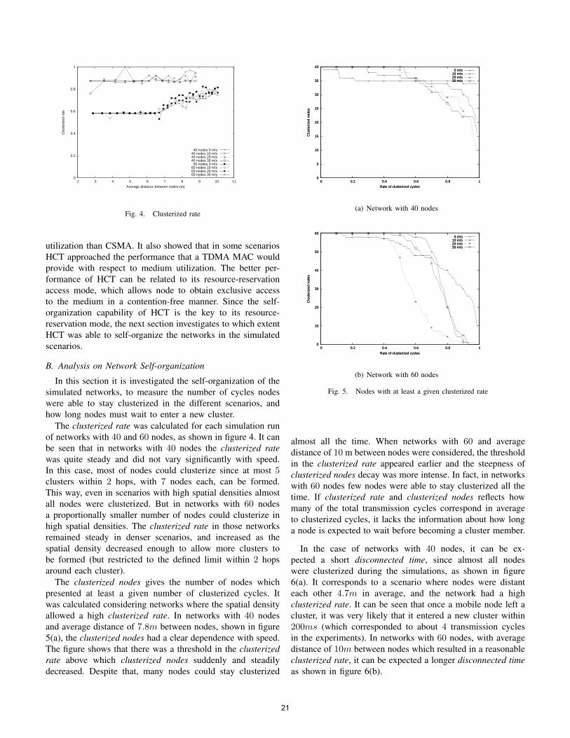
The rate of received frames obtained with HCT with particu-lar maximum speeds of nodes had a low variability in networkswith both 40 or 60 nodes. In both cases, the rate of receivedframes presented similar results with different speeds (from0m/s to 30m/s) as shown in figures 2(a) and 2(b). It must be

19

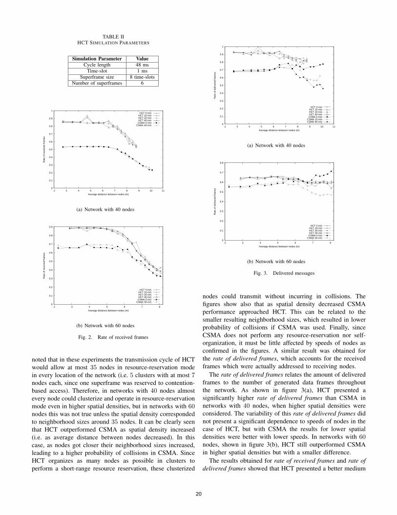
TABLE IIHCT SIMULATION PARAMETERS

Simulation Parameter ValueCycle length 48 ms

Time-slot 1 msSuperframe size 8 time-slots

Number of superframes 6

0

0.1

0.2

0.3

0.4

0.5

0.6

0.7

0.8

0.9

1

2 3 4 5 6 7 8 9 10 11

Rat

e of

rec

eive

d fr

ames

Average distance between nodes (m)

HCT 0 m/sHCT 10 m/sHCT 20 m/sHCT 40 m/sCSMA 0 m/s

CSMA 40 m/s

(a) Network with 40 nodes

0

0.1

0.2

0.3

0.4

0.5

0.6

0.7

0.8

0.9

2 3 4 5 6 7 8

Rat

e of

rec

eive

d fr

ames



CSMA 30 m/s

(b) Network with 60 nodes

Fig. 2. Rate of received frames

noted that in these experiments the transmission cycle of HCTwould allow at most 35 nodes in resource-reservation modein every location of the network (i.e. 5 clusters with at most 7nodes each, since one superframe was reserved to contention-based access). Therefore, in networks with 40 nodes almostevery node could clusterize and operate in resource-reservationmode even in higher spatial densities, but in networks with 60nodes this was not true unless the spatial density correspondedto neighborhood sizes around 35 nodes. It can be clearly seenthat HCT outperformed CSMA as spatial density increased(i.e. as average distance between nodes decreased). In thiscase, as nodes got closer their neighborhood sizes increased,leading to a higher probability of collisions in CSMA. SinceHCT organizes as many nodes as possible in clusters toperform a short-range resource reservation, these clusterized

0

0.1

0.2

0.3

0.4

0.5

0.6

0.7

0.8

0.9

1

2 3 4 5 6 7 8 9 10 11

Rat

e of

del

iver

ed fr

ames



CSMA 10 m/sCSMA 40 m/s


0

0.1

0.2

0.3

0.4

0.5

0.6

0.7

0.8

2 3 4 5 6 7 8

Rat

e of

del

iver

ed fr

ames



CSMA 30 m/s


Fig. 3. Delivered messages

nodes could transmit without incurring in collisions. Thefigures show also that as spatial density decreased CSMAperformance approached HCT. This can be related to thesmaller resulting neighborhood sizes, which resulted in lowerprobability of collisions if CSMA was used. Finally, sinceCSMA does not perform any resource-reservation nor self-organization, it must be little affected by speeds of nodes asconfirmed in the figures. A similar result was obtained forthe rate of delivered frames, which accounts for the receivedframes which were actually addressed to receiving nodes.

The rate of delivered frames relates the amount of deliveredframes to the number of generated data frames throughoutthe network. As shown in figure 3(a), HCT presented asignificantly higher rate of delivered frames than CSMA innetworks with 40 nodes, when higher spatial densities wereconsidered. The variability of this rate of delivered frames didnot present a significant dependence to speeds of nodes in thecase of HCT, but with CSMA the results for lower spatialdensities were better with lower speeds. In networks with 60nodes, shown in figure 3(b), HCT still outperformed CSMAin higher spatial densities but with a smaller difference.

The results obtained for rate of received frames and rate ofdelivered frames showed that HCT presented a better medium

20

0

0.2

0.4

0.6

0.8

1

2 3 4 5 6 7 8 9 10 11

Clu

ster

ized

rat

e


40 nodes 0 m/s40 nodes 10 m/s40 nodes 20 m/s40 nodes 30 m/s

60 nodes 0 m/s60 nodes 10 m/s60 nodes 20 m/s60 nodes 30 m/s

Fig. 4. Clusterized rate

utilization than CSMA. It also showed that in some scenariosHCT approached the performance that a TDMA MAC wouldprovide with respect to medium utilization. The better per-formance of HCT can be related to its resource-reservationaccess mode, which allows node to obtain exclusive accessto the medium in a contention-free manner. Since the self-organization capability of HCT is the key to its resource-reservation mode, the next section investigates to which extentHCT was able to self-organize the networks in the simulatedscenarios.

B. Analysis on Network Self-organization

In this section it is investigated the self-organization of thesimulated networks, to measure the number of cycles nodeswere able to stay clusterized in the different scenarios, andhow long nodes must wait to enter a new cluster.

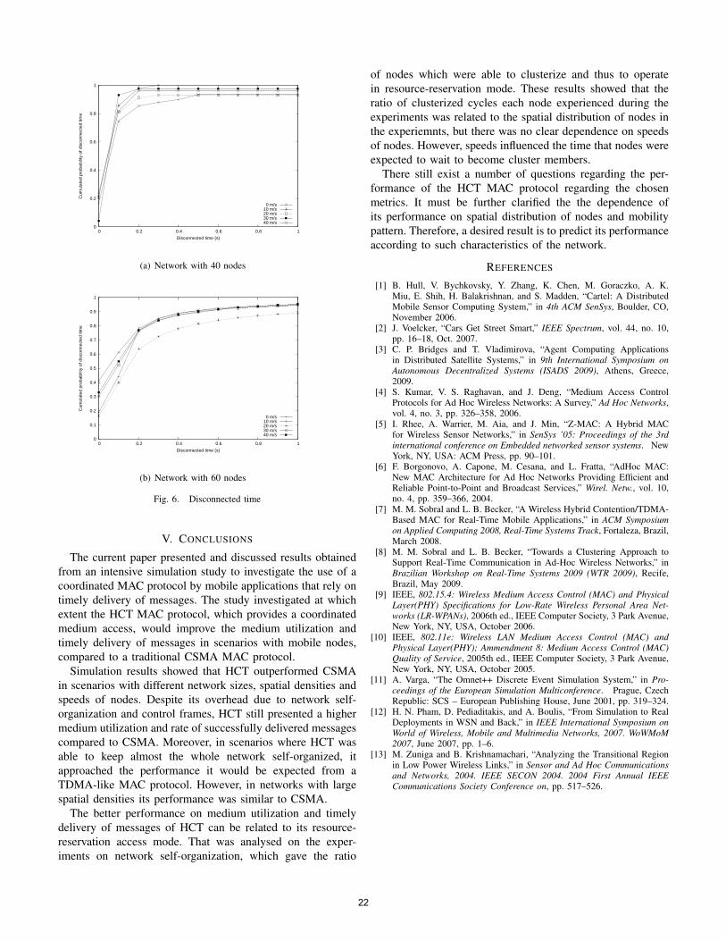
The clusterized rate was calculated for each simulation runof networks with 40 and 60 nodes, as shown in figure 4. It canbe seen that in networks with 40 nodes the clusterized ratewas quite steady and did not vary significantly with speed.In this case, most of nodes could clusterize since at most 5clusters within 2 hops, with 7 nodes each, can be formed.This way, even in scenarios with high spatial densities almostall nodes were clusterized. But in networks with 60 nodesa proportionally smaller number of nodes could clusterize inhigh spatial densities. The clusterized rate in those networksremained steady in denser scenarios, and increased as thespatial density decreased enough to allow more clusters tobe formed (but restricted to the defined limit within 2 hopsaround each cluster).

The clusterized nodes gives the number of nodes whichpresented at least a given number of clusterized cycles. Itwas calculated considering networks where the spatial densityallowed a high clusterized rate. In networks with 40 nodesand average distance of 7.8m between nodes, shown in figure5(a), the clusterized nodes had a clear dependence with speed.The figure shows that there was a threshold in the clusterizedrate above which clusterized nodes suddenly and steadilydecreased. Despite that, many nodes could stay clusterized

0

5

10

15

20

25

30

35

40

0 0.2 0.4 0.6 0.8 1

Clu

ster

ized

nod

es

Rate of clusterized cycles

0 m/s10 m/s20 m/s30 m/s

0

5

10

15

20

25

30

35

40

0 0.2 0.4 0.6 0.8 1

Clu

ster

ized

nod

es


0 m/s10 m/s20 m/s30 m/s


0

10

20

30

40

50

60

0 0.2 0.4 0.6 0.8 1

Clu

ster

ized

nod

es


0 m/s10 m/s20 m/s30 m/s

0

10

20

30

40

50

60

0 0.2 0.4 0.6 0.8 1

Clu

ster

ized

nod

es


0 m/s10 m/s20 m/s30 m/s


Fig. 5. Nodes with at least a given clusterized rate

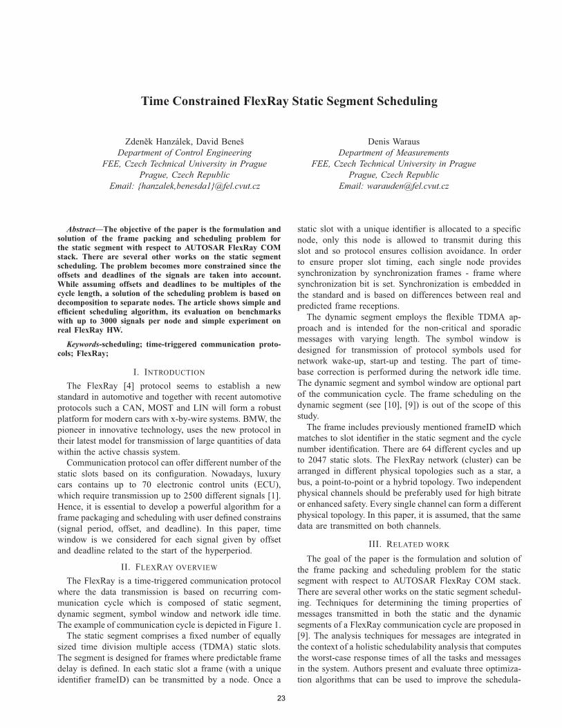
almost all the time. When networks with 60 and averagedistance of 10 m between nodes were considered, the thresholdin the clusterized rate appeared earlier and the steepness ofclusterized nodes decay was more intense. In fact, in networkswith 60 nodes few nodes were able to stay clusterized all thetime. If clusterized rate and clusterized nodes reflects howmany of the total transmission cycles correspond in averageto clusterized cycles, it lacks the information about how longa node is expected to wait before becoming a cluster member.

In the case of networks with 40 nodes, it can be ex-pected a short disconnected time, since almost all nodeswere clusterized during the simulations, as shown in figure6(a). It corresponds to a scenario where nodes were distanteach other 4.7m in average, and the network had a highclusterized rate. It can be seen that once a mobile node left acluster, it was very likely that it entered a new cluster within200ms (which corresponded to about 4 transmission cyclesin the experiments). In networks with 60 nodes, with averagedistance of 10m between nodes which resulted in a reasonableclusterized rate, it can be expected a longer disconnected timeas shown in figure 6(b).

21

0

0.2

0.4

0.6

0.8

1

0 0.2 0.4 0.6 0.8 1

Cum

ulat

ed p

roba

bilit

y of

dis

conn

ecte

d tim

e

Disconnected time (s)

0 m/s10 m/s20 m/s30 m/s40 m/s


0

0.1

0.2

0.3

0.4

0.5

0.6

0.7

0.8

0.9

1

0 0.2 0.4 0.6 0.8 1

Cum

ulat

ed p

roba

bilit

y of

dis

conn

ecte

d tim

e

Disconnected time (s)

0 m/s10 m/s20 m/s30 m/s40 m/s


Fig. 6. Disconnected time

V. CONCLUSIONS

The current paper presented and discussed results obtainedfrom an intensive simulation study to investigate the use of acoordinated MAC protocol by mobile applications that rely ontimely delivery of messages. The study investigated at whichextent the HCT MAC protocol, which provides a coordinatedmedium access, would improve the medium utilization andtimely delivery of messages in scenarios with mobile nodes,compared to a traditional CSMA MAC protocol.

Simulation results showed that HCT outperformed CSMAin scenarios with different network sizes, spatial densities andspeeds of nodes. Despite its overhead due to network self-organization and control frames, HCT still presented a highermedium utilization and rate of successfully delivered messagescompared to CSMA. Moreover, in scenarios where HCT wasable to keep almost the whole network self-organized, itapproached the performance it would be expected from aTDMA-like MAC protocol. However, in networks with largespatial densities its performance was similar to CSMA.

The better performance on medium utilization and timelydelivery of messages of HCT can be related to its resource-reservation access mode. That was analysed on the exper-iments on network self-organization, which gave the ratio

of nodes which were able to clusterize and thus to operatein resource-reservation mode. These results showed that theratio of clusterized cycles each node experienced during theexperiments was related to the spatial distribution of nodes inthe experiemnts, but there was no clear dependence on speedsof nodes. However, speeds influenced the time that nodes wereexpected to wait to become cluster members.

There still exist a number of questions regarding the per-formance of the HCT MAC protocol regarding the chosenmetrics. It must be further clarified the the dependence ofits performance on spatial distribution of nodes and mobilitypattern. Therefore, a desired result is to predict its performanceaccording to such characteristics of the network.

REFERENCES

[1] B. Hull, V. Bychkovsky, Y. Zhang, K. Chen, M. Goraczko, A. K.Miu, E. Shih, H. Balakrishnan, and S. Madden, “Cartel: A DistributedMobile Sensor Computing System,” in 4th ACM SenSys, Boulder, CO,November 2006.

[2] J. Voelcker, “Cars Get Street Smart,” IEEE Spectrum, vol. 44, no. 10,pp. 16–18, Oct. 2007.

[3] C. P. Bridges and T. Vladimirova, “Agent Computing Applicationsin Distributed Satellite Systems,” in 9th International Symposium onAutonomous Decentralized Systems (ISADS 2009), Athens, Greece,2009.

[4] S. Kumar, V. S. Raghavan, and J. Deng, “Medium Access ControlProtocols for Ad Hoc Wireless Networks: A Survey,” Ad Hoc Networks,vol. 4, no. 3, pp. 326–358, 2006.

[5] I. Rhee, A. Warrier, M. Aia, and J. Min, “Z-MAC: A Hybrid MACfor Wireless Sensor Networks,” in SenSys ’05: Proceedings of the 3rdinternational conference on Embedded networked sensor systems. NewYork, NY, USA: ACM Press, pp. 90–101.

[6] F. Borgonovo, A. Capone, M. Cesana, and L. Fratta, “AdHoc MAC:New MAC Architecture for Ad Hoc Networks Providing Efficient andReliable Point-to-Point and Broadcast Services,” Wirel. Netw., vol. 10,no. 4, pp. 359–366, 2004.

[7] M. M. Sobral and L. B. Becker, “A Wireless Hybrid Contention/TDMA-Based MAC for Real-Time Mobile Applications,” in ACM Symposiumon Applied Computing 2008, Real-Time Systems Track, Fortaleza, Brazil,March 2008.

[8] M. M. Sobral and L. B. Becker, “Towards a Clustering Approach toSupport Real-Time Communication in Ad-Hoc Wireless Networks,” inBrazilian Workshop on Real-Time Systems 2009 (WTR 2009), Recife,Brazil, May 2009.

[9] IEEE, 802.15.4: Wireless Medium Access Control (MAC) and PhysicalLayer(PHY) Specifications for Low-Rate Wireless Personal Area Net-works (LR-WPANs), 2006th ed., IEEE Computer Society, 3 Park Avenue,New York, NY, USA, October 2006.

[10] IEEE, 802.11e: Wireless LAN Medium Access Control (MAC) andPhysical Layer(PHY); Ammendment 8: Medium Access Control (MAC)Quality of Service, 2005th ed., IEEE Computer Society, 3 Park Avenue,New York, NY, USA, October 2005.

[11] A. Varga, “The Omnet++ Discrete Event Simulation System,” in Pro-ceedings of the European Simulation Multiconference. Prague, CzechRepublic: SCS – European Publishing House, June 2001, pp. 319–324.

[12] H. N. Pham, D. Pediaditakis, and A. Boulis, “From Simulation to RealDeployments in WSN and Back,” in IEEE International Symposium onWorld of Wireless, Mobile and Multimedia Networks, 2007. WoWMoM2007, June 2007, pp. 1–6.

[13] M. Zuniga and B. Krishnamachari, “Analyzing the Transitional Regionin Low Power Wireless Links,” in Sensor and Ad Hoc Communicationsand Networks, 2004. IEEE SECON 2004. 2004 First Annual IEEECommunications Society Conference on, pp. 517–526.

22

Time Constrained FlexRay Static Segment Scheduling

Zdenek Hanzálek, David BenešDepartment of Control Engineering

FEE, Czech Technical University in PraguePrague, Czech Republic

Email: {hanzalek,benesda1}@fel.cvut.cz

Denis WarausDepartment of Measurements

FEE, Czech Technical University in PraguePrague, Czech Republic

Email: [email protected]

Abstract—The objective of the paper is the formulation andsolution of the frame packing and scheduling problem forthe static segment with respect to AUTOSAR FlexRay COMstack. There are several other works on the static segmentscheduling. The problem becomes more constrained since theoffsets and deadlines of the signals are taken into account.While assuming offsets and deadlines to be multiples of thecycle length, a solution of the scheduling problem is based ondecomposition to separate nodes. The article shows simple andefficient scheduling algorithm, its evaluation on benchmarkswith up to 3000 signals per node and simple experiment onreal FlexRay HW.

Keywords-scheduling; time-triggered communication proto-cols; FlexRay;

I. INTRODUCTION

The FlexRay [4] protocol seems to establish a newstandard in automotive and together with recent automotiveprotocols such a CAN, MOST and LIN will form a robustplatform for modern cars with x-by-wire systems. BMW, thepioneer in innovative technology, uses the new protocol intheir latest model for transmission of large quantities of datawithin the active chassis system.

Communication protocol can offer different number of thestatic slots based on its configuration. Nowadays, luxurycars contains up to 70 electronic control units (ECU),which require transmission up to 2500 different signals [1].Hence, it is essential to develop a powerful algorithm for aframe packaging and scheduling with user defined constrains(signal period, offset, and deadline). In this paper, timewindow is we considered for each signal given by offsetand deadline related to the start of the hyperperiod.

II. FLEXRAY OVERVIEW

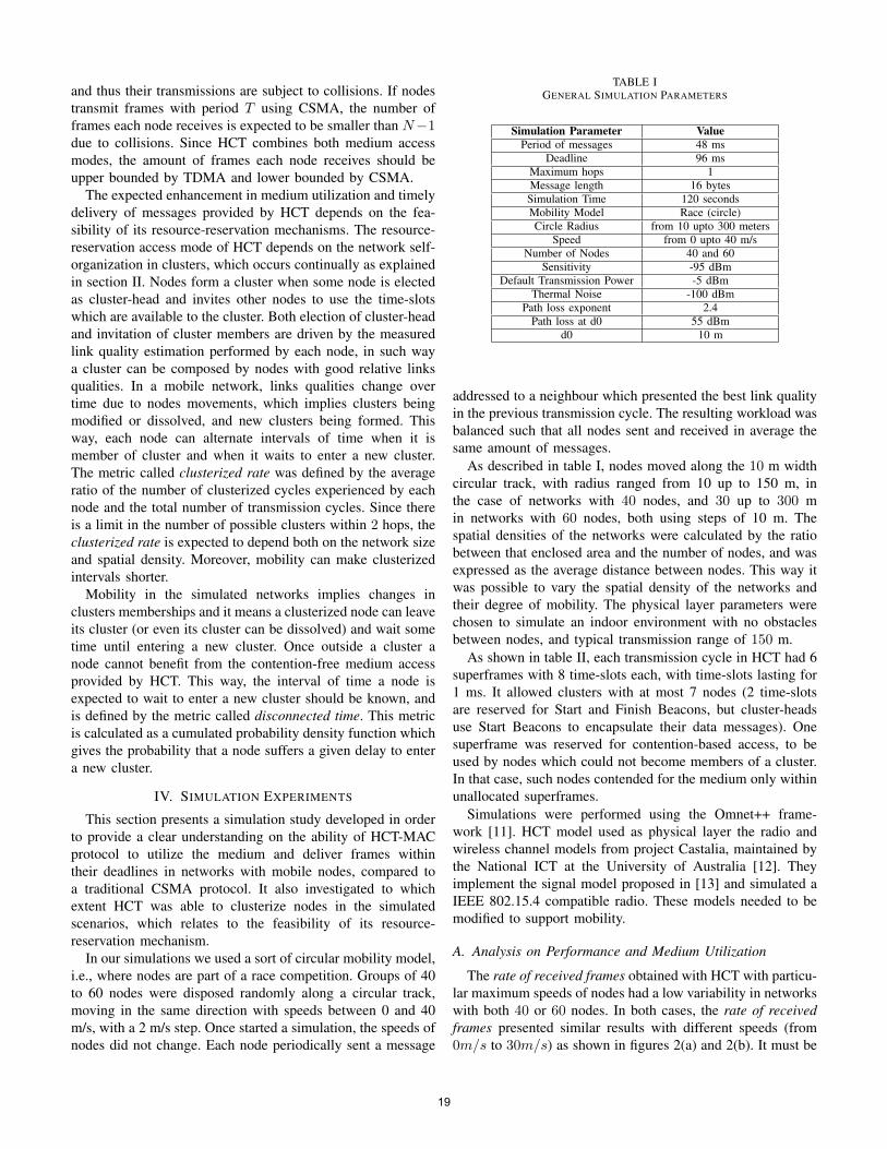
The FlexRay is a time-triggered communication protocolwhere the data transmission is based on recurring com-munication cycle which is composed of static segment,dynamic segment, symbol window and network idle time.The example of communication cycle is depicted in Figure 1.

The static segment comprises a fixed number of equallysized time division multiple access (TDMA) static slots.The segment is designed for frames where predictable framedelay is defined. In each static slot a frame (with a uniqueidentifier frameID) can be transmitted by a node. Once a

static slot with a unique identifier is allocated to a specificnode, only this node is allowed to transmit during thisslot and so protocol ensures collision avoidance. In orderto ensure proper slot timing, each single node providessynchronization by synchronization frames - frame wheresynchronization bit is set. Synchronization is embedded inthe standard and is based on differences between real andpredicted frame receptions.

The dynamic segment employs the flexible TDMA ap-proach and is intended for the non-critical and sporadicmessages with varying length. The symbol window isdesigned for transmission of protocol symbols used fornetwork wake-up, start-up and testing. The part of time-base correction is performed during the network idle time.The dynamic segment and symbol window are optional partof the communication cycle. The frame scheduling on thedynamic segment (see [10], [9]) is out of the scope of thisstudy.

The frame includes previously mentioned frameID whichmatches to slot identifier in the static segment and the cyclenumber identification. There are 64 different cycles and upto 2047 static slots. The FlexRay network (cluster) can bearranged in different physical topologies such as a star, abus, a point-to-point or a hybrid topology. Two independentphysical channels should be preferably used for high bitrateor enhanced safety. Every single channel can form a differentphysical topology. In this paper, it is assumed, that the samedata are transmitted on both channels.

III. RELATED WORK

The goal of the paper is the formulation and solution ofthe frame packing and scheduling problem for the staticsegment with respect to AUTOSAR FlexRay COM stack.There are several other works on the static segment schedul-ing. Techniques for determining the timing properties ofmessages transmitted in both the static and the dynamicsegments of a FlexRay communication cycle are proposed in[9]. The analysis techniques for messages are integrated inthe context of a holistic schedulability analysis that computesthe worst-case response times of all the tasks and messagesin the system. Authors present and evaluate three optimiza-tion algorithms that can be used to improve the schedula-

23

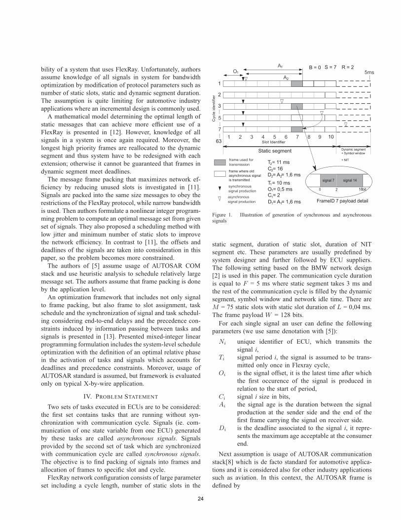
bility of a system that uses FlexRay. Unfortunately, authorsassume knowledge of all signals in system for bandwidthoptimization by modification of protocol parameters such asnumber of static slots, static and dynamic segment duration.The assumption is quite limiting for automotive industryapplications where an incremental design is commonly used.

A mathematical model determining the optimal length ofstatic messages that can achieve more efficient use of aFlexRay is presented in [12]. However, knowledge of allsignals in a system is once again required. Moreover, thelongest high priority frames are reallocated to the dynamicsegment and thus system have to be redesigned with eachextension; otherwise it cannot be guaranteed that frames indynamic segment meet deadlines.

The message frame packing that maximizes network ef-ficiency by reducing unused slots is investigated in [11].Signals are packed into the same size messages to obey therestrictions of the FlexRay protocol, while narrow bandwidthis used. Then authors formulate a nonlinear integer program-ming problem to compute an optimal message set from givenset of signals. They also proposed a scheduling method withlow jitter and minimum number of static slots to improvethe network efficiency. In contrast to [11], the offsets anddeadlines of the signals are taken into consideration in thispaper, so the problem becomes more constrained.

The authors of [5] assume usage of AUTOSAR COMstack and use heuristic analysis to schedule relatively largemessage set. The authors assume that frame packing is doneby the application level.

An optimization framework that includes not only signalto frame packing, but also frame to slot assignment, taskschedule and the synchronization of signal and task schedul-ing considering end-to-end delays and the precedence con-straints induced by information passing between tasks andsignals is presented in [13]. Presented mixed-integer linearprogramming formulation includes the system-level scheduleoptimization with the definition of an optimal relative phasein the activation of tasks and signals which accounts fordeadlines and precedence constraints. Moreover, usage ofAUTOSAR standard is assumed, but framework is evaluatedonly on typical X-by-wire application.

IV. PROBLEM STATEMENT

Two sets of tasks executed in ECUs are to be considered:the first set contains tasks that are running without syn-chronization with communication cycle. Signals (ie. com-munication of one state variable from one ECU) generatedby these tasks are called asynchronous signals. Signalsprovided by the second set of task which are synchronizedwith communication cycle are called synchronous signals.The objective is to find packing of signals into frames andallocation of frames to specific slot and cycle.

FlexRay network configuration consists of large parameterset including a cycle length, number of static slots in the

Figure 1. Illustration of generation of synchronous and asynchronoussignals

static segment, duration of static slot, duration of NITsegment etc. These parameters are usually predefined bysystem designer and further followed by ECU suppliers.The following setting based on the BMW network design[2] is used in this paper. The communication cycle durationis equal to F = 5 ms where static segment takes 3 ms andthe rest of the communication cycle is filled by the dynamicsegment, symbol window and network idle time. There areM = 75 static slots with static slot duration of L = 0,04 ms.The frame payload W = 128 bits.

For each single signal an user can define the followingparameters (we use same denotation with [5]):

Ni unique identifier of ECU, which transmits thesignal i,

Ti signal period i, the signal is assumed to be trans-mitted only once in Flexray cycle,

Oi is the signal offset, it is the latest time after whichthe first occurence of the signal is produced inrelation to the start of period,

Ci signal i size in bits,Ai the signal age is the duration between the signal

production at the sender side and the end of thefirst frame carrying the signal on receiver side.

Di is the deadline associated to the signal i, it repre-sents the maximum age acceptable at the consumerend.

Next assumption is usage of AUTOSAR communicationstack[8] which is de facto standard for automotive applica-tions and it is considered also for other industry applicationssuch as aviation. In this context, the AUTOSAR frame isdefined by

24

Qj unique ECU identifier, which transmits the framej,

Sj static slot identifier used for frame j,Rj the AUTOSAR frame repetition, which is the trans-

mission period of frame expressed as a multiple ofthe communication cycle with the constrains thatthe repetition takes its value in {2n|n ∈ N , n ≤ 6},

Bj the base cycle identifier - the first occurence of theframe j. Bj ≤ Rj .

Each single frame j is thus characterized by a tuplet{Qj, Sj , Bj , Rj}. The frame contains processing data units(PDU) where each consists of one or more signals. Anupdate bit can be defined for each PDU. It informs recipientswhether at least one signal in the PDU was updated or not.The signal can be contained in more than one PDU. InAUTOSAR context is defined that scheduling is static andcannot be changed during runtime.

It is further assumed, that maximal signal size cannotexceed data payload of the frame. It means that signal cannotbe split into two or more frames. Message fragmentation isensured by AUTOSAR FlexRay transport protocol layer [7].

By oversampling, the asynchronous signal is transformedto synchronous one with the following parameters:

Di = Ti = 2n · F + P + U

Oi = 0 (1)

where P is packing time - time from task request on signali transmission to the start of frame transmission and U isunpacking time.

Synchronous signals can keep deadline shorter than aperiod. In this case deadline is limited by the followingvalues

DSi ≥

{P + L+ U for 0 ≤ Oi − n · F ≤ P +M · L+ U

P + L+G+ U otherwise(2)

where n ∈ 1, 2, ..64, M is number of static slots, L isduration of the static slot, and G is duration of dynamicsegment, network idle time and symbolic window.

The Figure 1 depicts a situation where two signals aregenerated – synchronous one and asynchronous one. Theperiod of synchronous is set to 10 ms and 11 ms forasynchronous. Let us assume that, both signals have thedeadline equal to the period. In order to fulfill the deadlineconstraint, it is necessary to transmit both signals everysecond cycle, it means Rj = 21. In the fourth cycle ECUtransmits the same data twice due to oversampling of theasynchronous signal. However, this behavior is covered bypreviously mentioned update bit.

A. Message setThe scheduling approaches are applied to the modified

Society of Automotive Engineers (SAE) benchmark signalset.

The SAE report describes a set of signals sent betweenseven different subsystems in an electric car prototype.The Basic SAE signal set defines 53 sporadic and periodicsignals. A periodic message has a fixed period 5, 10, 100,1000 ms, and implicitly requires the latency to be less thanor equal to this period. Sporadic messages have latencyrequirements imposed by the application: for example, allmessages sent as a result of a driver action have a latencyrequirement of 20 ms. The reader is referred to the work ofKopetz [6] for more detailed benchmark description. Dueto the high FlexRay bandwitch (10Mb/s) and electronicequipment’s requirements in today’s cars we extended theSEA benchmark using NETCARBENCH[3] to:

• increase the number of signals while using the sameprobability distribution function of parameters - up to3000 signals per node are considered in this article,

• add parameters (such as offset).

B. Time constraints

In the first step, it is needed to find each signal pair{Ei, Hi} where E is earliest and H latest slot which can beused for transmission of the first occurrence of the signal i.The pair is given by

Ei = floor(P +Oi

F) ·M + (3)

+ min (ceil((P +Oi − floor(P+Oi

F) · F

L),M)

Hi = floor(P +Oi

F) ·M + (4)

+ min (floor(P +Oi +Di − floor(P+Oi

F) · F

L),M)

In order to simplify the scheduling problem, each node isscheduled separately, following decomposition in [11]. Forthis reason, we express {Oi, Di}, earliest and latest cycle totransmit signal i, as follows:

Oi = ceil(Ei

M) (5)

Di = floor(Hi

M) (6)

This simplifies our scenario, since offsets and deadlinescould be only multiples of the cycle length, because positionof signal within the cycle is insignificant with respectto position of signal within hyperperiod. This effectivelymeans, that we don’t care about assignment of particularID to the node, so it is not important, that the node has thefirst ID, or the last one.

25

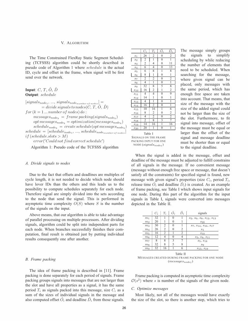
V. ALGORITHM

The Time Constrained FlexRay Static Segment Schedul-ing (TCFSSS) algorithm could be shortly described inpseudo code of Algorithm 1 where schedule is the actualID, cycle and offset in the frame, when signal will be firstsend over the network.

Input: C, T , O, DOutput: schedule

[signalsnode1, ..., signalsnodenumber of nodes] =

= divide signals to nodes(C, T, O, D)for (k = 1 ... number of nodes) do :

messagesnodek = frame packing(signalsnodek)optmessagesnodek = optimization(messagesnodek)schedulenodek = create schedule(optmessagesnodek)

schedule = [schedulenode1, ..., schedulenodenumber of nodes]

if (schedule.slots > M )error(′Could not find correct schedule′)

Algorithm 1: Pseudo code of the TCFSSS algorithm

A. Divide signals to nodes

Due to the fact that offsets and deadlines are multiples ofcycle length, it is not needed to decide which node shouldhave lover IDs than the others and this leads us to thepossibility to compute schedules separately for each node.Therefore signal are simply divided into the sets accordingto the node that send the signal. This is performed inasymptotic time complexity O(S) where S is the numberof the signals on the input.

Above means, that our algorithm is able to take advantageof parallel processing on multiple processors. After dividingsignals, algorithm could be split into independent parts foreach node. When branches successfully finishes their com-putation, final result is obtained just by putting individualresults consequently one after another.

B. Frame packing

The idea of frame packing is described in [11]. Framepacking is done separately for each period of signals. Framepacking groups signals into messages that are not larger thanthe slot and have all properties as a signal, it has the sameperiod Ti as signals packed into this message, size Ci as asum of the sizes of individual signals in the message andalso computed offset Oi and deadline Di from those signals.

Ci Ti Oi Di

s1 26 2 0 2s2 2 1 0 1s3 2 4 0 11s4 6 4 0 13s5 6 8 1 8s6 8 1 0 1s7 2 2 0 2s8 4 1 0 1s9 32 8 5 8s10 16 2 1 2s11 4 4 0 9s12 14 1 0 1s13 4 1 0 1s14 16 2 0 1s15 10 16 1 6s16 8 2 0 2s17 4 2 0 2s18 2 8 3 7s19 14 16 1 16s20 20 1 0 1

Table ISIGNALS ON THE FRAMEPACKING INPUT FOR ONE

NODE (signalsnode7)

The message simply groupsthe signals to simplifyscheduling by while reducingthe number of elements thatneed to be scheduled. Whensearching for the message,where given signal can beplaced, only messages withthe same period, which hasenough free space are takeninto account. That means, thatsize of the message with thesize of the added signal couldnot be larger than the size ofthe slot. Furthermore, to fitsignal into message, offset ofthe message must be equal orlarger than the offset of thesignal and message deadlinemust be shorter than or equalto the signal deadline.

When the signal is added in the message, offset anddeadline of the message must be adjusted to fulfill constrainsof all signals in the message. If no convenient message(message without enough free space or message, that doesn’tsatisfy all the constraints) for specified signal is found, newmessage with given signal’s properties (size Ci, period Ti,release time Oi and deadline Di) is created. As an exampleof frame packing, see Table I which shows input signals forone node. During this part of the algorithm for the inputsignals in Table I, signals were converted into messagesdepicted in the Table II.

Ci Ti Oi Di signalsm1 32 1 0 1 s2, s6, s8, s12, s13m2 20 1 0 1 s20m3 30 2 0 1 s7, s14, s16, s17m4 26 2 0 2 s1m5 16 2 1 2 s10m6 12 4 0 4 s3, s4, s11m7 8 8 3 7 s5, s18m8 32 8 5 8 s9m9 32 16 1 6 s15, s19

Table IIMESSAGES CREATED DURING FRAME PACKING FOR ONE NODE

(messagesnode7)

Frame packing is computed in asymptotic time complexityO(s2) where s is number of the signals of the given node.

C. Optimize messagesMost likely, not all of the messages would have exactly

the size of the slot, so there is another step, which tries to

26

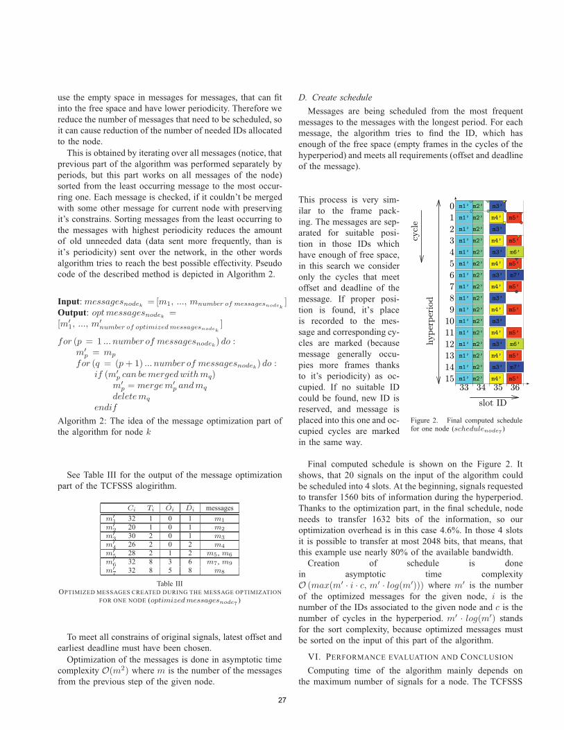
use the empty space in messages for messages, that can fitinto the free space and have lower periodicity. Therefore wereduce the number of messages that need to be scheduled, soit can cause reduction of the number of needed IDs allocatedto the node.

This is obtained by iterating over all messages (notice, thatprevious part of the algorithm was performed separately byperiods, but this part works on all messages of the node)sorted from the least occurring message to the most occur-ring one. Each message is checked, if it couldn’t be mergedwith some other message for current node with preservingit’s constrains. Sorting messages from the least occurring tothe messages with highest periodicity reduces the amountof old unneeded data (data sent more frequently, than isit’s periodicity) sent over the network, in the other wordsalgorithm tries to reach the best possible effectivity. Pseudocode of the described method is depicted in Algorithm 2.

Input: messagesnodek = [m1, ..., mnumber of messagesnodek]

Output: optmessagesnodek =[m′

1, ..., m′

number of optimizedmessagesnodek]

for (p = 1 ... number of messagesnodek) do :m′

p = mp

for (q = (p+ 1) ... number of messagesnodek) do :if (m′

p can bemergedwithmq)m′

p = mergem′

p andmq

deletemq

endif

Algorithm 2: The idea of the message optimization part ofthe algorithm for node k

See Table III for the output of the message optimizationpart of the TCFSSS alogirithm.

Ci Ti Oi Di messagesm′

132 1 0 1 m1

m′

220 1 0 1 m2

m′

330 2 0 1 m3

m′

426 2 0 2 m4

m′

528 2 1 2 m5, m6

m′

632 8 3 6 m7, m9

m′

732 8 5 8 m8

Table IIIOPTIMIZED MESSAGES CREATED DURING THE MESSAGE OPTIMIZATION

FOR ONE NODE (optimizedmessagesnode7)

To meet all constrains of original signals, latest offset andearliest deadline must have been chosen.

Optimization of the messages is done in asymptotic timecomplexity O(m2) where m is the number of the messagesfrom the previous step of the given node.

D. Create scheduleMessages are being scheduled from the most frequent

messages to the messages with the longest period. For eachmessage, the algorithm tries to find the ID, which hasenough of the free space (empty frames in the cycles of thehyperperiod) and meets all requirements (offset and deadlineof the message).

This process is very sim-ilar to the frame pack-ing. The messages are sep-arated for suitable posi-tion in those IDs whichhave enough of free space,in this search we consideronly the cycles that meetoffset and deadline of themessage. If proper posi-tion is found, it’s placeis recorded to the mes-sage and corresponding cy-cles are marked (becausemessage generally occu-pies more frames thanksto it’s periodicity) as oc-cupied. If no suitable IDcould be found, new ID isreserved, and message isplaced into this one and oc-cupied cycles are markedin the same way.

m5’

m4’

m2’

m1’

m2’

m4’

m2’

m5’

m3’

m3’m2’

m3’

m3’

m5’

m1’

m6’

m2’

m1’

m5’m1’

m1’

m2’

m2’m1’

m2’

m2’

m1’

m4’

m1’

m7’

m3’

m6’

m1’

m5’m1’

m7’

m4’

m3’

m5’

m1’

m5’

m1’

m3’

m1’

m1’

m2’

m2’

m4’

m1’

m5’

m4’

m4’m2’

m3’m1’

m4’

m2’

m2’

m2’

m2’

0

cycle

hyperperiod

slot ID

33 34 35 36

1

2

3

4

5

6

7

8

9

10

11

12

13

14

15

Figure 2. Final computed schedulefor one node (schedulenode7

)

Final computed schedule is shown on the Figure 2. Itshows, that 20 signals on the input of the algorithm couldbe scheduled into 4 slots. At the beginning, signals requestedto transfer 1560 bits of information during the hyperperiod.Thanks to the optimization part, in the final schedule, nodeneeds to transfer 1632 bits of the information, so ouroptimization overhead is in this case 4.6%. In those 4 slotsit is possible to transfer at most 2048 bits, that means, thatthis example use nearly 80% of the available bandwidth.

Creation of schedule is donein asymptotic time complexityO (max(m′ · i · c, m′ · log(m′))) where m′ is the numberof the optimized messages for the given node, i is thenumber of the IDs associated to the given node and c is thenumber of cycles in the hyperperiod. m′ · log(m′) standsfor the sort complexity, because optimized messages mustbe sorted on the input of this part of the algorithm.

VI. PERFORMANCE EVALUATION AND CONCLUSION

Computing time of the algorithm mainly depends onthe maximum number of signals for a node. The TCFSSS

27

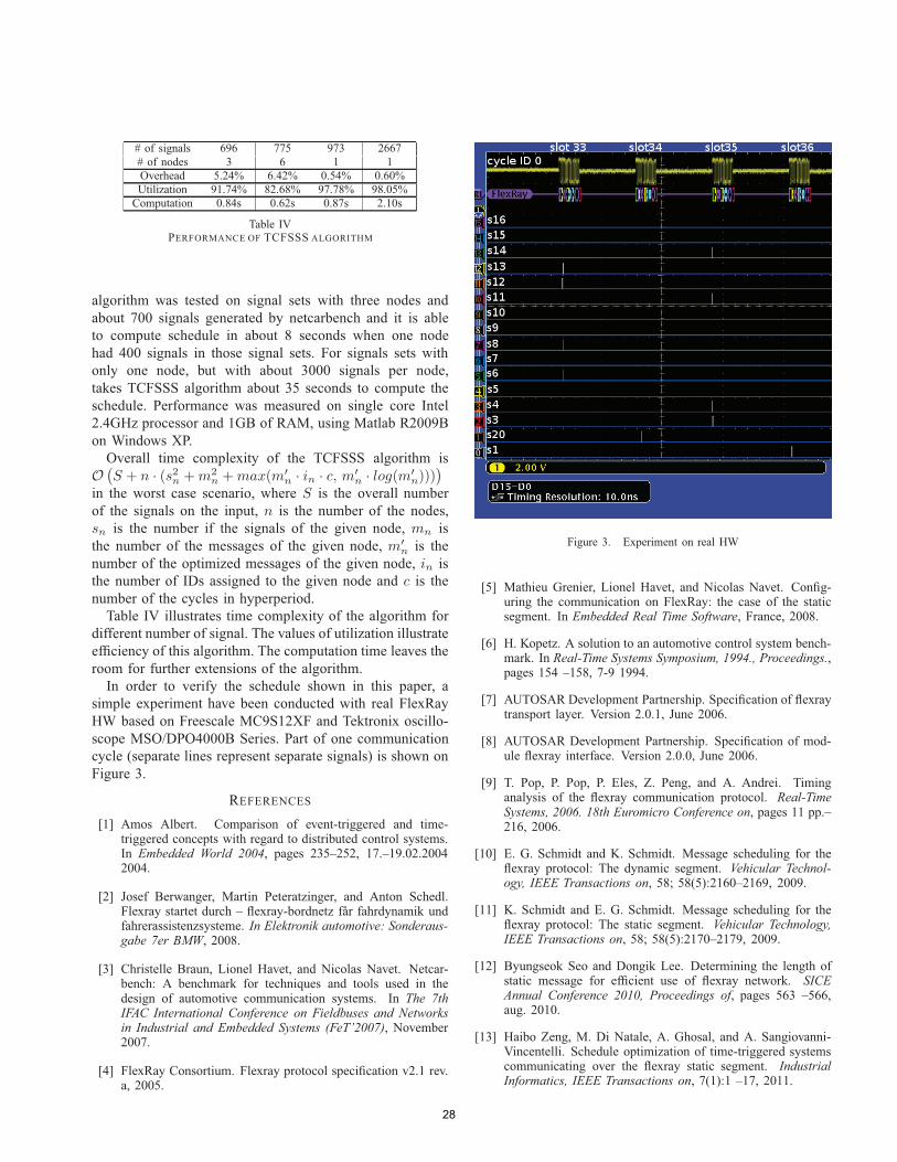
# of signals 696 775 973 2667# of nodes 3 6 1 1Overhead 5.24% 6.42% 0.54% 0.60%Utilization 91.74% 82.68% 97.78% 98.05%

Computation 0.84s 0.62s 0.87s 2.10s

Table IVPERFORMANCE OF TCFSSS ALGORITHM

algorithm was tested on signal sets with three nodes andabout 700 signals generated by netcarbench and it is ableto compute schedule in about 8 seconds when one nodehad 400 signals in those signal sets. For signals sets withonly one node, but with about 3000 signals per node,takes TCFSSS algorithm about 35 seconds to compute theschedule. Performance was measured on single core Intel2.4GHz processor and 1GB of RAM, using Matlab R2009Bon Windows XP.

Overall time complexity of the TCFSSS algorithm isO(S + n · (s2n +m2

n +max(m′

n · in · c, m′

n · log(m′

n))))

in the worst case scenario, where S is the overall numberof the signals on the input, n is the number of the nodes,sn is the number if the signals of the given node, mn isthe number of the messages of the given node, m′

n is thenumber of the optimized messages of the given node, in isthe number of IDs assigned to the given node and c is thenumber of the cycles in hyperperiod.

Table IV illustrates time complexity of the algorithm fordifferent number of signal. The values of utilization illustrateefficiency of this algorithm. The computation time leaves theroom for further extensions of the algorithm.

In order to verify the schedule shown in this paper, asimple experiment have been conducted with real FlexRayHW based on Freescale MC9S12XF and Tektronix oscillo-scope MSO/DPO4000B Series. Part of one communicationcycle (separate lines represent separate signals) is shown onFigure 3.

REFERENCES

[1] Amos Albert. Comparison of event-triggered and time-triggered concepts with regard to distributed control systems.In Embedded World 2004, pages 235–252, 17.–19.02.20042004.

[2] Josef Berwanger, Martin Peteratzinger, and Anton Schedl.Flexray startet durch – flexray-bordnetz får fahrdynamik undfahrerassistenzsysteme. In Elektronik automotive: Sonderaus-gabe 7er BMW, 2008.

[3] Christelle Braun, Lionel Havet, and Nicolas Navet. Netcar-bench: A benchmark for techniques and tools used in thedesign of automotive communication systems. In The 7thIFAC International Conference on Fieldbuses and Networksin Industrial and Embedded Systems (FeT’2007), November2007.

[4] FlexRay Consortium. Flexray protocol specification v2.1 rev.a, 2005.

Figure 3. Experiment on real HW

[5] Mathieu Grenier, Lionel Havet, and Nicolas Navet. Config-uring the communication on FlexRay: the case of the staticsegment. In Embedded Real Time Software, France, 2008.

[6] H. Kopetz. A solution to an automotive control system bench-mark. In Real-Time Systems Symposium, 1994., Proceedings.,pages 154 –158, 7-9 1994.

[7] AUTOSAR Development Partnership. Specification of flexraytransport layer. Version 2.0.1, June 2006.

[8] AUTOSAR Development Partnership. Specification of mod-ule flexray interface. Version 2.0.0, June 2006.

[9] T. Pop, P. Pop, P. Eles, Z. Peng, and A. Andrei. Timinganalysis of the flexray communication protocol. Real-TimeSystems, 2006. 18th Euromicro Conference on, pages 11 pp.–216, 2006.

[10] E. G. Schmidt and K. Schmidt. Message scheduling for theflexray protocol: The dynamic segment. Vehicular Technol-ogy, IEEE Transactions on, 58; 58(5):2160–2169, 2009.

[11] K. Schmidt and E. G. Schmidt. Message scheduling for theflexray protocol: The static segment. Vehicular Technology,IEEE Transactions on, 58; 58(5):2170–2179, 2009.

[12] Byungseok Seo and Dongik Lee. Determining the length ofstatic message for efficient use of flexray network. SICEAnnual Conference 2010, Proceedings of, pages 563 –566,aug. 2010.

[13] Haibo Zeng, M. Di Natale, A. Ghosal, and A. Sangiovanni-Vincentelli. Schedule optimization of time-triggered systemscommunicating over the flexray static segment. IndustrialInformatics, IEEE Transactions on, 7(1):1 –17, 2011.

28

The Possibility of Wireless Sensor Networks for Commercial Vehicle Load

Monitoring

Jieun Jung*, Byunghun Song

RFID/USN Convergence Center

Korea Electronics Technology Institute

Gyeonggi-do, Republic of Korea

{jejung, bhsong}@keti.re.kr

Sooyeol Park

IT Convergence Research Center

Innosensing Corporation

Seoul, Republic of Korea

[email protected]

Abstract—It is of great importance to be able to monitor and

enforce vehicle weight limits for road authorities involved in

almost all aspects of transportation and pavement engineering.

For the active control of additional weight carried by

overloaded vehicles, essential IT technologies such as sensors,

measurement, and data processing have been applied. The

integration of vehicle load monitoring systems with Wireless

Sensor Networks (WSN) technology has a possibility of

reducing installation efforts and costs, and enabling the quick

and easy configuration of data acquisition and control systems.

In this paper, we try to verify that WSN technology can replace

the wiring sensor applications for vehicle monitoring issues.

The WSN-based system includes: inclinometer sensors which

measure variation of inclination values with load changes;, an

Access Point (AP) that logs the data collected from all these

sensors;, and a weight estimation algorithm. To reach the goal,

we performed an experiment with real deployment and

estimated the weight of trucks with an error of less than 3%.

The result shows that it is possible to adopt WSN for

commercial vehicle load monitoring.

Keywords-component; vehicle, inclinometer, WSN, weight

estimation, inclinometer sensor

I. INTRODUCTION

Recently telematic technologies used for vehicle information have provided a number of practical services, such as vehicle/traffic tracking, vehicle/road safety, and entertainment services. [1] To start with, vehicle/traffic tracking services are already deployed on a commercial scale, and drivers on the move can be informed of their location, movement, and status in real-time by using mobile systems such as navigation systems, cell phones and so on. Furthermore, electromechanical sensors embedded in vehicles, such as pressure, acceleration, and temperature sensors help drivers to maintain the safety of surrounding vehicles.

However, vehicle accidents on the road have been on the increase, especially accidents caused by huge commercial vehicles including trucks and, trailers, and these are becoming a big issue nowadays. According to an analysis of traffic accidents in the Republic of Korea in 2008, 4.7 % of vehicle accidents were caused by huge commercial vehicles, but they caused 12.5% of death from traffic accidents. This

reveals that accidents involving huge commercial vehicles are more likely to cause severe results. [2]

With the development of the distribution industry, more active control of overloading vehicles also becomes necessary for the management of highways and bridges. Overloading is one of the biggest elements which have a great influence on the deterioration of this SOC (Social Overhead Capital). When vehicles containing dangerous chemicals or fire risk materials overturn, this can even bring unexpected aftereffects. Hence, it is of great importance for the maintenance and operation of the road and bridge infrastructure to monitor and prevent vehicle overloading. Vehicle information, which is the basis of the successful creation of safety traffic environments, should be both collected and analyzed.

Various studies on monitoring over-weight vehicles have shown the benefits of monitoring them. At present, all road authorities use either stationary vehicle scales along the route or Weight-In-Motion (WIM) systems at toll plazas for vehicle load enforcement, although it involves expensive installation and calibration procedures. Firstly, static weight stations are inefficient in that they force vehicles to enter the stations and wait for the process in a queue. [3] To resolve this problem, mobile weighing systems have also been introduced and installed everywhere with no limitations. However, there still require vehicles on the move to stop.

Lastly, WIM systems are designed to capture and record vehicle axle weights and gross vehicle weights when they drive over in-pavement sensors such as road cells. Unlike the above static weight stations, they do not require the subject vehicle travelling in traffic lanes to stop. However, it is still challenging to calculate weight accurately without any vehicle information such as fuel type, year, model and so on. Furthermore, WIM systems are highly sensitive to electromagnetic disturbances caused mostly by lightning strikes in the vicinity of the equipment. [4, 5]

In a different approach, weighing systems embedded in the vehicles have also been designed. [6] However, the weighing systems implemented using wired communication methods have difficulties in wiring and configuration constraints. Vehicles such as cargo trucks also have trouble disassembling part of their system because they fold their back trailers in case they are empty. Therefore, we surveyed

29

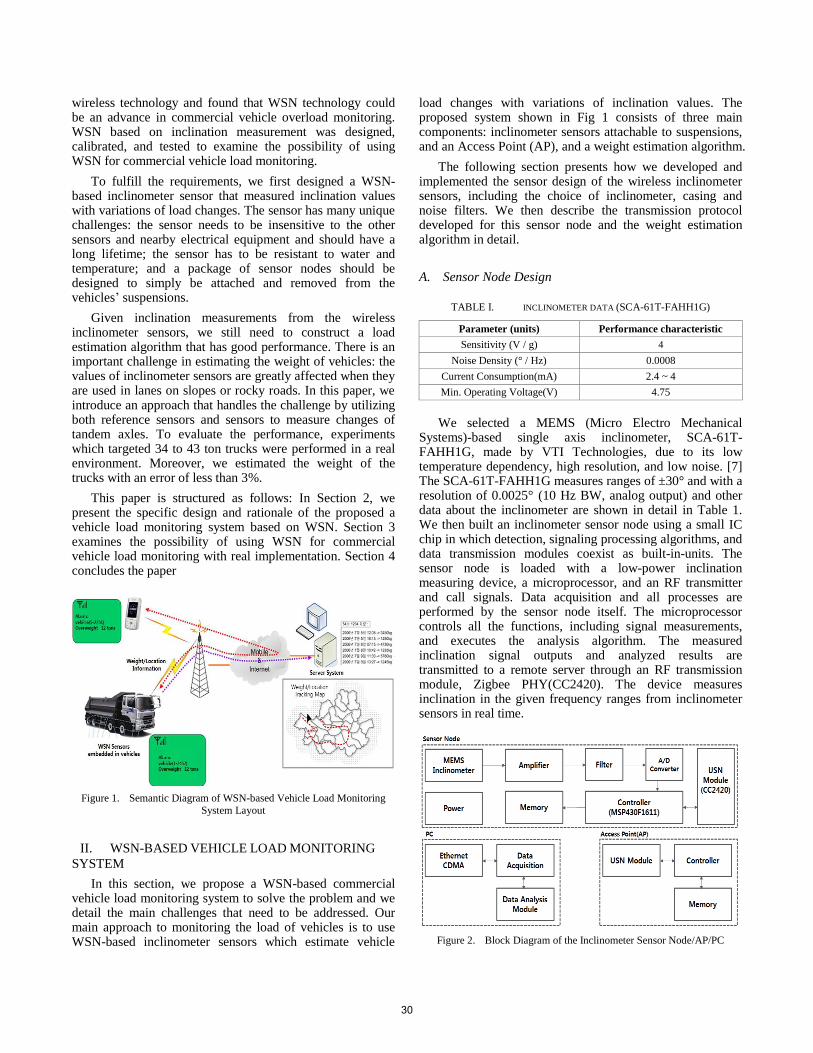
wireless technology and found that WSN technology could be an advance in commercial vehicle overload monitoring. WSN based on inclination measurement was designed, calibrated, and tested to examine the possibility of using WSN for commercial vehicle load monitoring.

To fulfill the requirements, we first designed a WSN-based inclinometer sensor that measured inclination values with variations of load changes. The sensor has many unique challenges: the sensor needs to be insensitive to the other sensors and nearby electrical equipment and should have a long lifetime; the sensor has to be resistant to water and temperature; and a package of sensor nodes should be designed to simply be attached and removed from the vehicles’ suspensions.

Given inclination measurements from the wireless inclinometer sensors, we still need to construct a load estimation algorithm that has good performance. There is an important challenge in estimating the weight of vehicles: the values of inclinometer sensors are greatly affected when they are used in lanes on slopes or rocky roads. In this paper, we introduce an approach that handles the challenge by utilizing both reference sensors and sensors to measure changes of tandem axles. To evaluate the performance, experiments which targeted 34 to 43 ton trucks were performed in a real environment. Moreover, we estimated the weight of the trucks with an error of less than 3%.

This paper is structured as follows: In Section 2, we present the specific design and rationale of the proposed a vehicle load monitoring system based on WSN. Section 3 examines the possibility of using WSN for commercial vehicle load monitoring with real implementation. Section 4 concludes the paper

Figure 1. Semantic Diagram of WSN-based Vehicle Load Monitoring

System Layout

II. WSN-BASED VEHICLE LOAD MONITORING

SYSTEM

In this section, we propose a WSN-based commercial vehicle load monitoring system to solve the problem and we detail the main challenges that need to be addressed. Our main approach to monitoring the load of vehicles is to use WSN-based inclinometer sensors which estimate vehicle

load changes with variations of inclination values. The proposed system shown in Fig 1 consists of three main components: inclinometer sensors attachable to suspensions, and an Access Point (AP), and a weight estimation algorithm.

The following section presents how we developed and implemented the sensor design of the wireless inclinometer sensors, including the choice of inclinometer, casing and noise filters. We then describe the transmission protocol developed for this sensor node and the weight estimation algorithm in detail.

A. Sensor Node Design

TABLE I. INCLINOMETER DATA (SCA-61T-FAHH1G)

Parameter (units) Performance characteristic

Sensitivity (V / g) 4

Noise Density (° / Hz) 0.0008

Current Consumption(mA) 2.4 ~ 4

Min. Operating Voltage(V) 4.75

We selected a MEMS (Micro Electro Mechanical

Systems)-based single axis inclinometer, SCA-61T-FAHH1G, made by VTI Technologies, due to its low temperature dependency, high resolution, and low noise. [7] The SCA-61T-FAHH1G measures ranges of ±30° and with a resolution of 0.0025° (10 Hz BW, analog output) and other data about the inclinometer are shown in detail in Table 1. We then built an inclinometer sensor node using a small IC chip in which detection, signaling processing algorithms, and data transmission modules coexist as built-in-units. The sensor node is loaded with a low-power inclination measuring device, a microprocessor, and an RF transmitter and call signals. Data acquisition and all processes are performed by the sensor node itself. The microprocessor controls all the functions, including signal measurements, and executes the analysis algorithm. The measured inclination signal outputs and analyzed results are transmitted to a remote server through an RF transmission module, Zigbee PHY(CC2420). The device measures inclination in the given frequency ranges from inclinometer sensors in real time.

Figure 2. Block Diagram of the Inclinometer Sensor Node/AP/PC

30

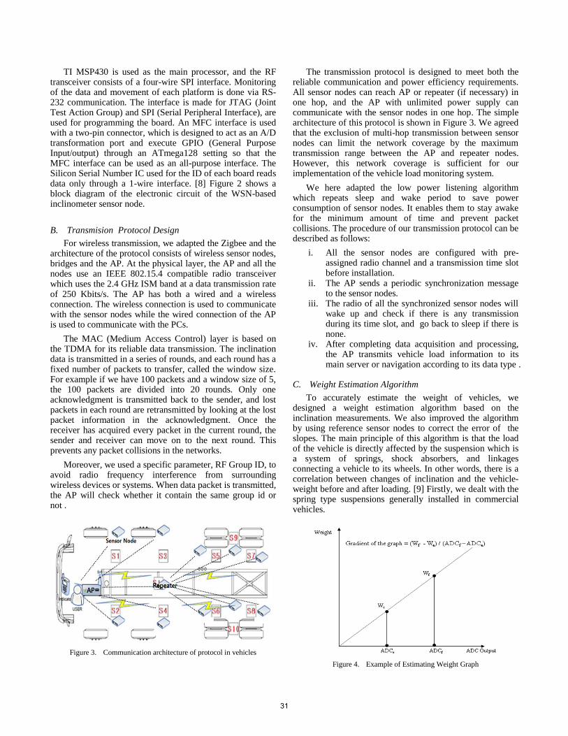
TI MSP430 is used as the main processor, and the RF transceiver consists of a four-wire SPI interface. Monitoring of the data and movement of each platform is done via RS-232 communication. The interface is made for JTAG (Joint Test Action Group) and SPI (Serial Peripheral Interface), are used for programming the board. An MFC interface is used with a two-pin connector, which is designed to act as an A/D transformation port and execute GPIO (General Purpose Input/output) through an ATmega128 setting so that the MFC interface can be used as an all-purpose interface. The Silicon Serial Number IC used for the ID of each board reads data only through a 1-wire interface. [8] Figure 2 shows a block diagram of the electronic circuit of the WSN-based inclinometer sensor node.

B. Transmision Protocol Design

For wireless transmission, we adapted the Zigbee and the architecture of the protocol consists of wireless sensor nodes, bridges and the AP. At the physical layer, the AP and all the nodes use an IEEE 802.15.4 compatible radio transceiver which uses the 2.4 GHz ISM band at a data transmission rate of 250 Kbits/s. The AP has both a wired and a wireless connection. The wireless connection is used to communicate with the sensor nodes while the wired connection of the AP is used to communicate with the PCs.

The MAC (Medium Access Control) layer is based on the TDMA for its reliable data transmission. The inclination data is transmitted in a series of rounds, and each round has a fixed number of packets to transfer, called the window size. For example if we have 100 packets and a window size of 5, the 100 packets are divided into 20 rounds. Only one acknowledgment is transmitted back to the sender, and lost packets in each round are retransmitted by looking at the lost packet information in the acknowledgment. Once the receiver has acquired every packet in the current round, the sender and receiver can move on to the next round. This prevents any packet collisions in the networks.

Moreover, we used a specific parameter, RF Group ID, to avoid radio frequency interference from surrounding wireless devices or systems. When data packet is transmitted, the AP will check whether it contain the same group id or not .

Figure 3. Communication architecture of protocol in vehicles

The transmission protocol is designed to meet both the reliable communication and power efficiency requirements. All sensor nodes can reach AP or repeater (if necessary) in one hop, and the AP with unlimited power supply can communicate with the sensor nodes in one hop. The simple architecture of this protocol is shown in Figure 3. We agreed that the exclusion of multi-hop transmission between sensor nodes can limit the network coverage by the maximum transmission range between the AP and repeater nodes. However, this network coverage is sufficient for our implementation of the vehicle load monitoring system.

We here adapted the low power listening algorithm which repeats sleep and wake period to save power consumption of sensor nodes. It enables them to stay awake for the minimum amount of time and prevent packet collisions. The procedure of our transmission protocol can be described as follows:

i. All the sensor nodes are configured with pre-assigned radio channel and a transmission time slot before installation.

ii. The AP sends a periodic synchronization message to the sensor nodes.

iii. The radio of all the synchronized sensor nodes will wake up and check if there is any transmission during its time slot, and go back to sleep if there is none.

iv. After completing data acquisition and processing, the AP transmits vehicle load information to its main server or navigation according to its data type .

C. Weight Estimation Algorithm

To accurately estimate the weight of vehicles, we designed a weight estimation algorithm based on the inclination measurements. We also improved the algorithm by using reference sensor nodes to correct the error of the slopes. The main principle of this algorithm is that the load of the vehicle is directly affected by the suspension which is a system of springs, shock absorbers, and linkages connecting a vehicle to its wheels. In other words, there is a correlation between changes of inclination and the vehicle-weight before and after loading. [9] Firstly, we dealt with the spring type suspensions generally installed in commercial vehicles.

Figure 4. Example of Estimating Weight Graph

31

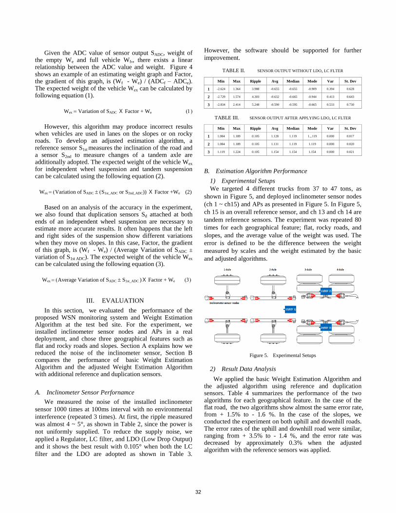
Given the ADC value of sensor output SADC, weight of the empty We and full vehicle Wf,, there exists a linear relationship between the ADC value and weight. Figure 4 shows an example of an estimating weight graph and Factor, the gradient of this graph, is (Wf - We) / (ADCf – ADCe). The expected weight of the vehicle Wex can be calculated by following equation (1).

Wex Variation of SADC ⅩFactor + We

However, this algorithm may produce incorrect results when vehicles are used in lanes on the slopes or on rocky roads. To develop an adjusted estimation algorithm, a reference sensor S1st measures the inclination of the road and a sensor S2nd to measure changes of a tandem axle are additionally adopted. The expected weight of the vehicle Wex for independent wheel suspension and tandem suspension can be calculated using the following equation (2).

Wex Variation of SADC S1st_ADC or S2nd_ADC)) ⅩFactor +We (2)

Based on an analysis of the accuracy in the experiment, we also found that duplication sensors Sd attached at both ends of an independent wheel suspension are necessary to estimate more accurate results. It often happens that the left and right sides of the suspension show different variations when they move on slopes. In this case, Factor, the gradient of this graph, is (Wf - We) / (Average Variation of SADC ± variation of S1st ADC). The expected weight of the vehicle Wex can be calculated using the following equation (3).

Wex Average Variation of SADC S1st_ADC )ⅩFactor + We

III. EVALUATION

In this section, we evaluated the performance of the proposed WSN monitoring system and Weight Estimation Algorithm at the test bed site. For the experiment, we installed inclinometer sensor nodes and APs in a real deployment, and chose three geographical features such as flat and rocky roads and slopes. Section A explains how we reduced the noise of the inclinometer sensor, Section B compares the performance of basic Weight Estimation Algorithm and the adjusted Weight Estimation Algorithm with additional reference and duplication sensors.

A. Inclinometer Sensor Perfornamce

We measured the noise of the installed inclinometer

sensor 1000 times at 100ms interval with no environmental

interference (repeated 3 times). At first, the ripple measured

was almost 4 ~ 5°, as shown in Table 2, since the power is

not uniformly supplied. To reduce the supply noise, we

applied a Regulator, LC filter, and LDO (Low Drop Output)

and it shows the best result with 0.105° when both the LC

filter and the LDO are adopted as shown in Table 3.

However, the software should be supported for further

improvement.

TABLE II. SENSOR OUTPUT WITHOUT LDO, LC FLTER

Min Max Ripple Avg Median Mode Var St. Dev

1 -2.624 1.364 3.988 -0.655 -0.655 -0.909 0.394 0.628

2 -2.729 1.574 4.303 -0.632 -0.665 -0.944 0.413 0.643

3 -2.834 2.414 5.248 -0.590 -0.595 -0.665 0.533 0.730

TABLE III. SENSOR OUTPUT AFTER APPLYING LDO, LC FLTER

Min Max Ripple Avg Median Mode Var St. Dev

1 1.084 1.189 0.105 1.128 1.119 1.,.119 0.000 0.017

2 1.084 1.189 0.105 1.131 1.119 1.119 0.000 0.020

3 1.119 1.224 0.105 1.154 1.154 1.154 0.000 0.021

B. Estimation Algorithm Performance

1) Experimental Setups

We targeted 4 different trucks from 37 to 47 tons, as

shown in Figure 5, and deployed inclinometer sensor nodes

(ch 1 ~ ch15) and APs as presented in Figure 5. In Figure 5,

ch 15 is an overall reference sensor, and ch 13 and ch 14 are

tandem reference sensors. The experiment was repeated 80

times for each geographical feature; flat, rocky roads, and

slopes, and the average value of the weight was used. The

error is defined to be the difference between the weight

measured by scales and the weight estimated by the basic

and adjusted algorithms.

Figure 5. Experimental Setups

2) Result Data Analysis

We applied the basic Weight Estimation Algorithm and the adjusted algorithm using reference and duplication sensors. Table 4 summarizes the performance of the two algorithms for each geographical feature. In the case of the flat road, the two algorithms show almost the same error rate, from + 1.5% to - 1.6 %. In the case of the slopes, we conducted the experiment on both uphill and downhill roads. The error rates of the uphill and downhill road were similar, ranging from + 3.5% to - 1.4 %, and the error rate was decreased by approximately 0.3% when the adjusted algorithm with the reference sensors was applied.

32

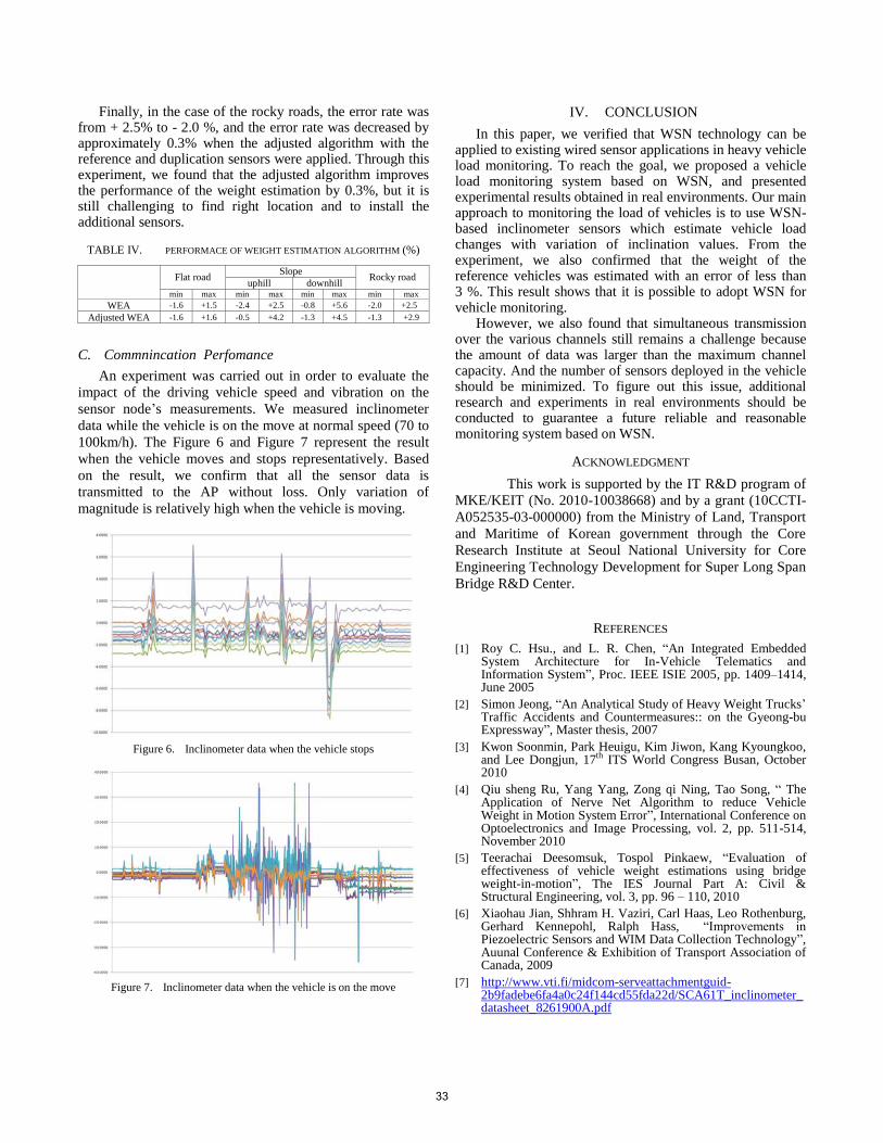
Finally, in the case of the rocky roads, the error rate was from + 2.5% to - 2.0 %, and the error rate was decreased by approximately 0.3% when the adjusted algorithm with the reference and duplication sensors were applied. Through this experiment, we found that the adjusted algorithm improves the performance of the weight estimation by 0.3%, but it is still challenging to find right location and to install the additional sensors.

TABLE IV. PERFORMACE OF WEIGHT ESTIMATION ALGORITHM (%)

Flat road

Slope Rocky road

uphill downhill min max min max min max min max

WEA -1.6 +1.5 -2.4 +2.5 -0.8 +5.6 -2.0 +2.5

Adjusted WEA -1.6 +1.6 -0.5 +4.2 -1.3 +4.5 -1.3 +2.9

C. Commnincation Perfomance

An experiment was carried out in order to evaluate the

impact of the driving vehicle speed and vibration on the

sensor node’s measurements. We measured inclinometer

data while the vehicle is on the move at normal speed (70 to

100km/h). The Figure 6 and Figure 7 represent the result

when the vehicle moves and stops representatively. Based

on the result, we confirm that all the sensor data is

transmitted to the AP without loss. Only variation of

magnitude is relatively high when the vehicle is moving.

Figure 6. Inclinometer data when the vehicle stops

Figure 7. Inclinometer data when the vehicle is on the move

IV. CONCLUSION

In this paper, we verified that WSN technology can be applied to existing wired sensor applications in heavy vehicle load monitoring. To reach the goal, we proposed a vehicle load monitoring system based on WSN, and presented experimental results obtained in real environments. Our main approach to monitoring the load of vehicles is to use WSN-based inclinometer sensors which estimate vehicle load changes with variation of inclination values. From the experiment, we also confirmed that the weight of the reference vehicles was estimated with an error of less than 3 %. This result shows that it is possible to adopt WSN for vehicle monitoring.

However, we also found that simultaneous transmission over the various channels still remains a challenge because the amount of data was larger than the maximum channel capacity. And the number of sensors deployed in the vehicle should be minimized. To figure out this issue, additional research and experiments in real environments should be conducted to guarantee a future reliable and reasonable monitoring system based on WSN.

ACKNOWLEDGMENT

This work is supported by the IT R&D program of

MKE/KEIT (No. 2010-10038668) and by a grant (10CCTI-

A052535-03-000000) from the Ministry of Land, Transport

and Maritime of Korean government through the Core

Research Institute at Seoul National University for Core

Engineering Technology Development for Super Long Span

Bridge R&D Center.

REFERENCES

[1] Roy C. Hsu., and L. R. Chen, “An Integrated Embedded System Architecture for In-Vehicle Telematics and Information System”, Proc. IEEE ISIE 2005, pp. 1409–1414, June 2005

[2] Simon Jeong, “An Analytical Study of Heavy Weight Trucks’ Traffic Accidents and Countermeasures:: on the Gyeong-bu Expressway”, Master thesis, 2007

[3] Kwon Soonmin, Park Heuigu, Kim Jiwon, Kang Kyoungkoo, and Lee Dongjun, 17th ITS World Congress Busan, October 2010

[4] Qiu sheng Ru, Yang Yang, Zong qi Ning, Tao Song, “ The Application of Nerve Net Algorithm to reduce Vehicle Weight in Motion System Error”, International Conference on Optoelectronics and Image Processing, vol. 2, pp. 511-514, November 2010

[5] Teerachai Deesomsuk, Tospol Pinkaew, “Evaluation of effectiveness of vehicle weight estimations using bridge weight-in-motion”, The IES Journal Part A: Civil & Structural Engineering, vol. 3, pp. 96 – 110, 2010

[6] Xiaohau Jian, Shhram H. Vaziri, Carl Haas, Leo Rothenburg, Gerhard Kennepohl, Ralph Hass, “Improvements in Piezoelectric Sensors and WIM Data Collection Technology”, Auunal Conference & Exhibition of Transport Association of Canada, 2009

[7] http://www.vti.fi/midcom-serveattachmentguid-2b9fadebe6fa4a0c24f144cd55fda22d/SCA61T_inclinometer_datasheet_8261900A.pdf

33

http://www.vti.fi/midcom-serveattachmentguid-2b9fadebe6fa4a0c24f144cd55fda22d/SCA61T_inclinometer_datasheet_8261900A.pdf



[8] Sukwon choi, Jieun Jung, Byunghun Song, and Sooyel Park, “Possibility of Wireless Sensor Networks for Outside Exposed Gas Pipeline Monitoring”, International Conference on Information Processing in Sensor Networks(IPSN) RealWIN Workshop, 2011

[9] Nicola Amati, Andrea Festini, Luigi Pelizza, Andrea Tonoli, “Dynamic modeling and experimental validation of three wheeled titling vehicles”, International Journal of Vehicle Mechanics and Mobility Special Issue, vol. 49, 2011

34

Real-time routing for low-latency 802.15.4 control networks

Koen Holtman, Peter van der Stok Philips Research, Eindhoven

High Tech Campus 34, 5656AE Eindhoven, the Netherlands {koen.holtman, peter.van.der.stok}@philips.com

Abstract In many applications of wireless control networks, the latency of message delivery is an important consideration. In a lighting control network where a light switch sends a wireless message to a lamp, a worst case end-to-end la-tency of 200 ms or better is desired, so that the working of the switch feels 'immediate' to the end user. This paper studies the probability that latency deadlines of a few hundred ms are exceeded. We use a 802.15.4 test net-work, located in a real-life office environment, to evaluate and compare the effects of several re-try and re-routing strategies. Testing under realistic conditions, in an office environment when people are present, is important to ac-curately determine worst case latency performance as ex-perienced by end users. At night, without any people in the building, performance is much better than during the day. In order to accurately observe the effect of different strategies, test runs lasting at least a week are needed. We find that retrying message delivery via a single deli-very route is sub-optimal. Keeping a set of two or more candidate routes for subsequent re-tries greatly improves worst-case latency.

1 Introduction A wireless control network differs from the more com-monly considered wireless sensor network (WSN) because it incorporates actuators in addition to sensors. Whereas in most WSN designs, the object is to get all sensing data forwarded to a central (logging) location for later analysis, in a wireless control network the object is to control actua-tors based on data from close-by sensors. Home and office control systems are important applications of wireless con-trol networks. The low cost of wireless sensor nodes, and their ability to run on batteries, makes it feasible to equip rooms with many sensors, which can be used to increase both comfort and energy efficiency. The reliability and latency of a wireless building control system must be just as good as that of the wired system that it replaces. Consider the case where a lamp in a room is wirelessly connected to a switch on the wall. In such a setup, it is not the average end-to-end latency that will be important for the quality perception of the user, but the worst-case latency. If the latency is too high too often, the system will break the ‘immediacy’ mental model that the user has for light switches, which negatively impacts the user experience and ultimately the user acceptance. Our design goal is to minimize the probability that 200 ms la-

tency is exceeded. As a rule of thumb in user interface de-sign, 200 ms latency is still short enough that the user can accept the relation between stimulus and response as ‘im-mediate’. Contrary to most publications we are less concerned with the maximum achievable throughput, average-case latency, or scalability of the routing algorithm. We expect that most communications in building control will not need more than 2 hops, with 4 hops being exceptional. We therefore focus on quality improvement of the 1-hop and 2-hop cas-es, which represent the bulk of the wireless control com-munication in the building. We concentrate on the effects of multipath fading which lead to unexpected link failures of very good links during the day time. Effects coming from interference caused by the high density of nodes are not investigated. Therefore, the measurements concentrate on a relatively low number of nodes reflecting the node and message density we ex-pect for building control

2 Measurements in literature This paper is motivated by measured communication be-haviour in buildings with occupants. In the literature measurements on wireless communication have been done to measure: Point to point communication, Sharing the medium between multiple senders, and Routing over a large dynamic network. This section summarizes the main published results as introduction to our routing sugges-tions to improve the probability that packets arrive in time (within their deadline). A naïve model of transmission by an omni-directional an-tenna in empty space, states that the strength of the signal decreases with the square of the distance [9]. Unfortu-nately, space is not empty but is populated with reflectors and absorbers of the RF signal. Reflections from surfaces can meet the original signal with a slightly different phase thus reducing or completely removing the signal. Report [9] shows that most simple propagation models used in simulations do not correctly represent the transmission as measured in situ. Measurements of the communication quality between a single sender and a receiver indicate that there are usually three regions: (1) a clear region with little or no reception losses, (2) a transitional region where packet loss ranges from a few percent to complete loss unrelated to the transmission distance, and (3) a region where almost no packets are received. Over time the link quality fluctuates as well. These phe-nomena are reported in [1][2]. The clear region for IEEE 802.15.4 [3] is reported to be on average between 3 and 15 meters in [5][6][8], where in some cases the signal had

35

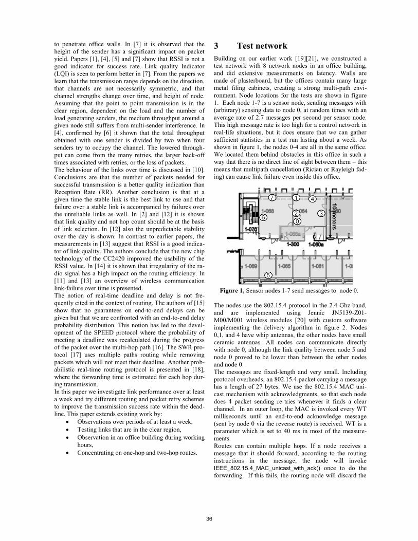
to penetrate office walls. In [7] it is observed that the height of the sender has a significant impact on packet yield. Papers [1], [4], [5] and [7] show that RSSI is not a good indicator for success rate. Link quality Indicator (LQI) is seen to perform better in [7]. From the papers we learn that the transmission range depends on the direction, that channels are not necessarily symmetric, and that channel strengths change over time, and height of node. Assuming that the point to point transmission is in the clear region, dependent on the load and the number of load generating senders, the medium throughput around a given node still suffers from multi-sender interference. In [4], confirmed by [6] it shown that the total throughput obtained with one sender is divided by two when four senders try to occupy the channel. The lowered through-put can come from the many retries, the larger back-off times associated with retries, or the loss of packets. The behaviour of the links over time is discussed in [10]. Conclusions are that the number of packets needed for successful transmission is a better quality indication than Reception Rate (RR). Another conclusion is that at a given time the stable link is the best link to use and that failure over a stable link is accompanied by failures over the unreliable links as well. In [2] and [12] it is shown that link quality and not hop count should be at the basis of link selection. In [12] also the unpredictable stability over the day is shown. In contrast to earlier papers, the measurements in [13] suggest that RSSI is a good indica-tor of link quality. The authors conclude that the new chip technology of the CC2420 improved the usability of the RSSI value. In [14] it is shown that irregularity of the ra-dio signal has a high impact on the routing efficiency. In [11] and [13] an overview of wireless communication link-failure over time is presented. The notion of real-time deadline and delay is not fre-quently cited in the context of routing. The authors of [15] show that no guarantees on end-to-end delays can be given but that we are confronted with an end-to-end delay probability distribution. This notion has led to the devel-opment of the SPEED protocol where the probability of meeting a deadline was recalculated during the progress of the packet over the multi-hop path [16]. The SWR pro-tocol [17] uses multiple paths routing while removing packets which will not meet their deadline. Another prob-abilistic real-time routing protocol is presented in [18], where the forwarding time is estimated for each hop dur-ing transmission. In this paper we investigate link performance over at least a week and try different routing and packet retry schemes to improve the transmission success rate within the dead-line. This paper extends existing work by:

� Observations over periods of at least a week, � Testing links that are in the clear region, � Observation in an office building during working

hours, � Concentrating on one-hop and two-hop routes.

3 Test network Building on our earlier work [19][21], we constructed a test network with 8 network nodes in an office building, and did extensive measurements on latency. Walls are made of plasterboard, but the offices contain many large metal filing cabinets, creating a strong multi-path envi-ronment. Node locations for the tests are shown in figure 1. Each node 1-7 is a sensor node, sending messages with (arbitrary) sensing data to node 0, at random times with an average rate of 2.7 messages per second per sensor node. This high message rate is too high for a control network in real-life situations, but it does ensure that we can gather sufficient statistics in a test run lasting about a week. As shown in figure 1, the nodes 0-4 are all in the same office. We located them behind obstacles in this office in such a way that there is no direct line of sight between them – this means that multipath cancellation (Rician or Rayleigh fad-ing) can cause link failure even inside this office.

Figure 1, Sensor nodes 1-7 send messages to node 0.

The nodes use the 802.15.4 protocol in the 2.4 Ghz band, and are implemented using Jennic JN5139-Z01-M00/M001 wireless modules [20] with custom software implementing the delivery algorithm in figure 2. Nodes 0,1, and 4 have whip antennas, the other nodes have small ceramic antennas. All nodes can communicate directly with node 0, although the link quality between node 5 and node 0 proved to be lower than between the other nodes and node 0. The messages are fixed-length and very small. Including protocol overheads, an 802.15.4 packet carrying a message has a length of 27 bytes. We use the 802.15.4 MAC uni-cast mechanism with acknowledgments, so that each node does 4 packet sending re-tries whenever it finds a clear channel. In an outer loop, the MAC is invoked every WT milliseconds until an end-to-end acknowledge message (sent by node 0 via the reverse route) is received. WT is a parameter which is set to 40 ms in most of the measure-ments. Routes can contain multiple hops. If a node receives a message that it should forward, according to the routing instructions in the message, the node will invoke IEEE_802.15.4_MAC_unicast_with_ack() once to do the forwarding. If this fails, the routing node will discard the

36

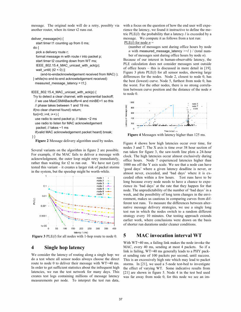
message. The original node will do a retry, possibly via another router, when its timer t2 runs out. deliver_message(m) {

start timer t1 counting up from 0 ms; do {

pick a delivery route r; format message m with route r into packet p; start timer t2 counting down from WT ms;IEEE_802.15.4_MAC_unicast_with_ack(p); wait_until( (t2 < 0) ||

(end-to-endacknowledgement received from MAC) ); } while(no end-to-end acknowledgement received)

measured_message_latency = t1;}

IEEE_802.15.4_MAC_unicast_with_ack(p) { Try to detect a clear channel, with exponential backoff;

// we use MaxCSMABackoffs=4 and minBE=1 so this // phase takes between 1 and 19 ms.

if(no clear channel found) return; for(i=0; i<4; i++) {

use radio to send packet p; // takes ~2 ms use radio to listen for MAC acknowledgement packet; // takes ~1 ms

if(valid MAC acknowledgement packet heard) break; } }

Figure 2 Message delivery algorithm used by nodes.

Several variants on the algorithm in figure 2 are possible. For example, if the MAC fails to deliver a message with acknowledgment, the outer loop might retry immediately, rather than waiting for t2 to run out. We have not (yet) tested this variant – it creates a larger risk of packet storms in the system, but the speedup might be worth-while.

Figure 3 PLE(l) for all nodes with 1-hop route to node 0.

4 Single hop latency We consider the latency of routing along a single hop: we do a test where all sensor nodes always choose the direct route to node 0 to deliver their message with WT=40 ms. In order to get sufficient statistics about the infrequent high latencies, we run the test network for many days. This creates test logs containing millions of message latency measurements per node. To interpret the test run data,

with a focus on the question of how the end user will expe-rience the latency, we found it instructive to define the me-tric PLE(l): the probability that a latency l is exceeded by a message. We compute it as follows from a test run: PLE(l) for node n =

(number of messages sent during office hours by node n with measured_message_latency >=l ) / (total num-ber of messages sent during office hours by node n).

Because of our interest in human-observable latency, the PLE calculation does not consider messages sent outside of office hours – this is discussed in more detail in [19]. Figure 3 plots PLE(l) for all sensor nodes, showing large differences for the nodes. Node 2, closest to node 0, has the best (lowest) curve. Node 5, furthest from node 0, has the worst. For the other nodes, there is no strong correla-tion between curve position and the distance of the node n to node 0.

Figure 4 Messages with latency higher than 125 ms.

Figure 4 shows how high latencies occur over time, for nodes 3 and 7. The X axis is time over 38 hour section of run taken for figure 3, the saw-tooth line plots a 24-hour clock. The high latencies occur almost exclusively during office hours. Node 7 experienced latencies higher than 1000 ms off the Y axis scale. We see that a node can have ‘good days’ where a given latency deadline is never, or almost never, exceeded, and ‘bad days’ where it is ex-ceeded often within a few hours. Test runs have to be long because every node needs to have a chance to expe-rience its ‘bad days’ at the rate that they happen for that node. The unpredictability of the number of ‘bad days’ in a week, and the possibility of long term changes in the envi-ronment, makes us cautious in comparing curves from dif-ferent test runs. To measure the differences between alter-native message delivery strategies, we use a single long test run in which the nodes switch to a random different strategy every 10 minutes. Our testing approach extends earlier work, where conclusions were drawn on the basis of shorter run durations under cleaner conditions.

5 MAC invocation interval WT With WT=40 ms, a failing link makes the node invoke the MAC, every 40 ms, sending at most 4 packets. So if a link is failing, WT=40 ms generally leads to a PHY pack-et sending rate of 100 packets per second, until success. This is an excessively high rate which may lead to packet storms. In [21], we used a 5-node test-bed to investigate the effect of varying WT. Some indicative results from [21] are shown in figure 5. Node 4 in the test bed used was far away from node 0, for this node we see an im-

37

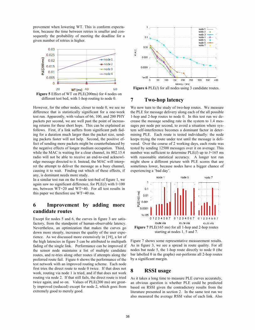
provement when lowering WT. This is conform expecta-tion, because the time between retries is smaller and con-sequently the probability of meeting the deadline for a given number of retries is higher.

Figure 5 Effect of WT on PLE(200ms) for 4 nodes on

different test bed, with 1-hop routing to node 0. However, for the other nodes, closer to node 0, we see no difference that is statistically significant for a one-week test run. Apparently, with values of 66, 100, and 200 PHY packets per second, we are well past the point of increas-ing returns for these short hops. This can be explained as follows. First, if a link suffers from significant path fad-ing for a duration much larger than the packet size, send-ing packets faster will not help. Second, the positive ef-fect of sending more packets might be counterbalanced by the negative effects of longer medium occupation. Third, while the MAC is waiting for a clear channel, its 802.15.4 radio will not be able to receive an end-to-end acknowl-edge message directed to it. Instead, the MAC will interp-ret the attempt to deliver the message as a busy channel, causing it to wait. Finding out which of these effects, if any, is dominant needs more study. In a similar test run on the 8-node test-bed of figure 1, we again saw no significant difference, for PLE(l) with l>100 ms, between WT=20 and WT=40. For all test results in this paper we therefore use WT=40 ms.

6 Improvement by adding more candidate routes Except for nodes 5 and 6, the curves in figure 3 are satis-factory, from the standpoint of human-observable latency. Nevertheless, an optimization that makes the curves go down more steeply, increases the quality of the user expe-rience. As we discussed more extensively in [19], a lot of the high latencies in figure 3 can be attributed to multipath fading of the single link. Performance can be improved if the sensor node maintains a list of multiple candidate routes, and re-tries along other routes if attempts along the preferred route fail. Figure 6 shows the performance of the test network with an improved routing scheme. Each node first tries the direct route to node 0 twice. If that does not work, routing via node 1 is tried, and if that does not work routing via node 2. If that still fails, the direct route is tried twice again, and so on. Values of PLE(200 ms) are great-ly improved (reduced) except for node 2, which goes from extremely good to merely good.

Figure 6 PLE(l) for all nodes using 3 candidate routes.

7 Two-hop latency We now turn to the study of two-hop routes. We measure the PLE for message delivery along each of the all possible 1-hop and 2-hop routes to node 0. In this test run we de-crease the message sending rate in the system to 1.4 mes-sages per node per second, to avoid a situation where sys-tem self-interference becomes a dominant factor in deter-mining PLE. Each route is tested individually: the node keeps trying the route under test until the message is deli-vered. Over the course of 2 working days, each route was tested by sending 12500 messages over it on average. This number was sufficient to determine PLE(l) up to l=165 ms with reasonable statistical accuracy. A longer test run might show a different picture with PLE scores that are sometimes lower, because nodes have a bigger chance of experiencing a ‘bad day’.

Figure 7 PLE(165 ms) for all 1-hop and 2-hop routes

starting at nodes 1, 5 and 7. Figure 7 shows some representative measurement results. As in figure 3, we see a spread in route quality. For all nodes but node 5, the 1-hop route directly to node 0 (the bar labelled 0 in the graphs) out-performs all 2-hop routes by a significant margin.

8 RSSI usage As it takes a long time to measure PLE curves accurately, an obvious question is whether PLE could be predicted based on RSSI given the contradictory results from the literature presented in section 2. In the same test run we also measured the average RSSI value of each link. Also

38

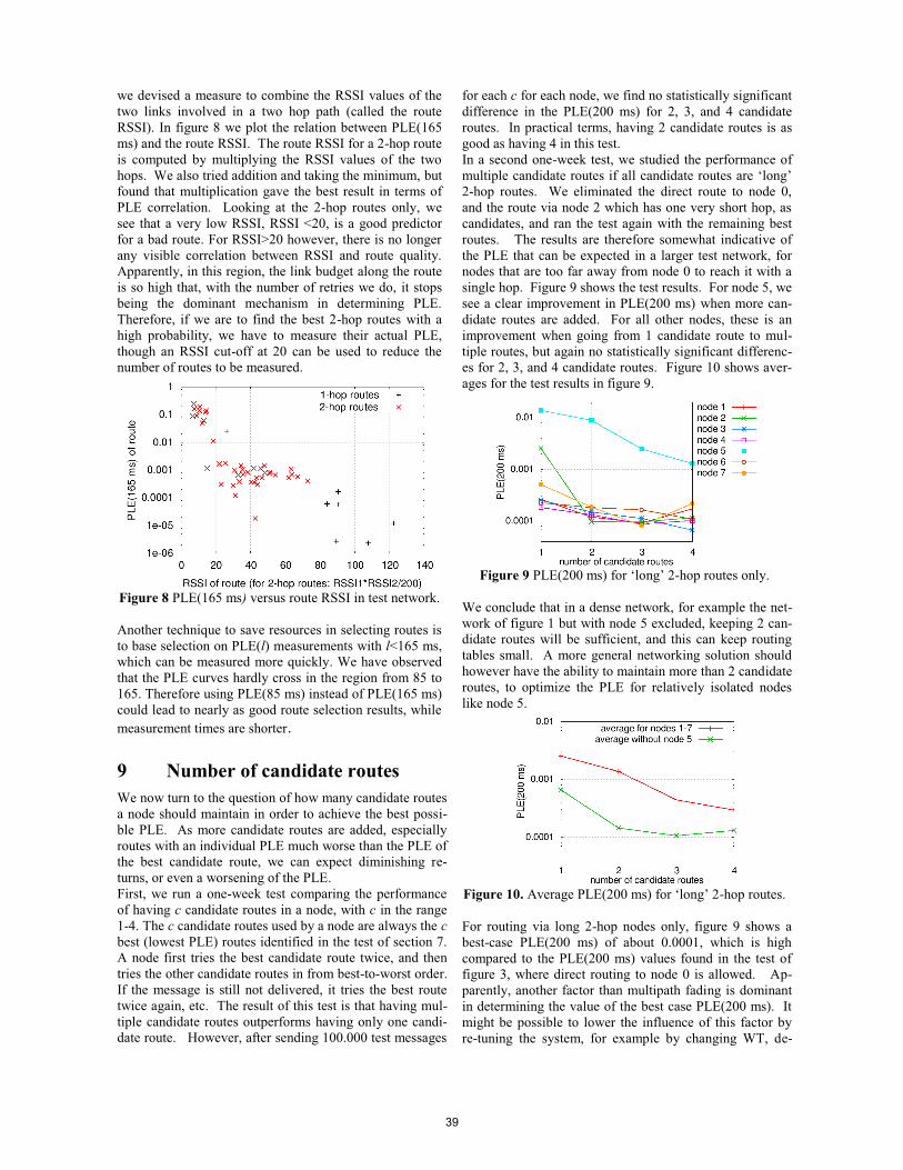
we devised a measure to combine the RSSI values of the two links involved in a two hop path (called the route RSSI). In figure 8 we plot the relation between PLE(165 ms) and the route RSSI. The route RSSI for a 2-hop route is computed by multiplying the RSSI values of the two hops. We also tried addition and taking the minimum, but found that multiplication gave the best result in terms of PLE correlation. Looking at the 2-hop routes only, we see that a very low RSSI, RSSI <20, is a good predictor for a bad route. For RSSI>20 however, there is no longer any visible correlation between RSSI and route quality. Apparently, in this region, the link budget along the route is so high that, with the number of retries we do, it stops being the dominant mechanism in determining PLE. Therefore, if we are to find the best 2-hop routes with a high probability, we have to measure their actual PLE, though an RSSI cut-off at 20 can be used to reduce the number of routes to be measured.

Figure 8 PLE(165 ms) versus route RSSI in test network.

Another technique to save resources in selecting routes is to base selection on PLE(l) measurements with l<165 ms, which can be measured more quickly. We have observed that the PLE curves hardly cross in the region from 85 to 165. Therefore using PLE(85 ms) instead of PLE(165 ms) could lead to nearly as good route selection results, while measurement times are shorter.

9 Number of candidate routes We now turn to the question of how many candidate routes a node should maintain in order to achieve the best possi-ble PLE. As more candidate routes are added, especially routes with an individual PLE much worse than the PLE of the best candidate route, we can expect diminishing re-turns, or even a worsening of the PLE. First, we run a one-week test comparing the performance of having c candidate routes in a node, with c in the range 1-4. The c candidate routes used by a node are always the c best (lowest PLE) routes identified in the test of section 7. A node first tries the best candidate route twice, and then tries the other candidate routes in from best-to-worst order. If the message is still not delivered, it tries the best route twice again, etc. The result of this test is that having mul-tiple candidate routes outperforms having only one candi-date route. However, after sending 100.000 test messages

for each c for each node, we find no statistically significant difference in the PLE(200 ms) for 2, 3, and 4 candidate routes. In practical terms, having 2 candidate routes is as good as having 4 in this test. In a second one-week test, we studied the performance of multiple candidate routes if all candidate routes are ‘long’ 2-hop routes. We eliminated the direct route to node 0, and the route via node 2 which has one very short hop, as candidates, and ran the test again with the remaining best routes. The results are therefore somewhat indicative of the PLE that can be expected in a larger test network, for nodes that are too far away from node 0 to reach it with a single hop. Figure 9 shows the test results. For node 5, we see a clear improvement in PLE(200 ms) when more can-didate routes are added. For all other nodes, these is an improvement when going from 1 candidate route to mul-tiple routes, but again no statistically significant differenc-es for 2, 3, and 4 candidate routes. Figure 10 shows aver-ages for the test results in figure 9.

Figure 9 PLE(200 ms) for ‘long’ 2-hop routes only.

We conclude that in a dense network, for example the net-work of figure 1 but with node 5 excluded, keeping 2 can-didate routes will be sufficient, and this can keep routing tables small. A more general networking solution should however have the ability to maintain more than 2 candidate routes, to optimize the PLE for relatively isolated nodes like node 5.

Figure 10. Average PLE(200 ms) for ‘long’ 2-hop routes. For routing via long 2-hop nodes only, figure 9 shows a best-case PLE(200 ms) of about 0.0001, which is high compared to the PLE(200 ms) values found in the test of figure 3, where direct routing to node 0 is allowed. Ap-parently, another factor than multipath fading is dominant in determining the value of the best case PLE(200 ms). It might be possible to lower the influence of this factor by re-tuning the system, for example by changing WT, de-

39

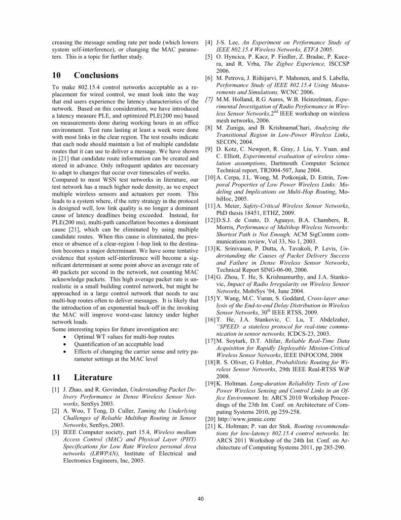
creasing the message sending rate per node (which lowers system self-interference), or changing the MAC parame-ters. This is a topic for further study.

10 Conclusions To make 802.15.4 control networks acceptable as a re-placement for wired control, we must look into the way that end users experience the latency characteristics of the network. Based on this consideration, we have introduced a latency measure PLE, and optimized PLE(200 ms) based on measurements done during working hours in an office environment. Test runs lasting at least a week were done with most links in the clear region. The test results indicate that each node should maintain a list of multiple candidate routes that it can use to deliver a message. We have shown in [21] that candidate route information can be created and stored in advance. Only infrequent updates are necessary to adapt to changes that occur over timescales of weeks. Compared to most WSN test networks in literature, our test network has a much higher node density, as we expect multiple wireless sensors and actuators per room. This leads to a system where, if the retry strategy in the protocol is designed well, low link quality is no longer a dominant cause of latency deadlines being exceeded. Instead, for PLE(200 ms), multi-path cancellation becomes a dominant cause [21], which can be eliminated by using multiple candidate routes. When this cause is eliminated, the pres-ence or absence of a clear-region 1-hop link to the destina-tion becomes a major determinant. We have some tentative evidence that system self-interference will become a sig-nificant determinant at some point above an average rate of 40 packets per second in the network, not counting MAC acknowledge packets. This high average packet rate is un-realistic in a small building control network, but might be approached in a large control network that needs to use multi-hop routes often to deliver messages. It is likely that the introduction of an exponential back-off in the invoking the MAC will improve worst-case latency under higher network loads. Some interesting topics for future investigation are:

� Optimal WT values for multi-hop routes � Quantification of an acceptable load � Effects of changing the carrier sense and retry pa-

rameter settings at the MAC level

11 Literature [1] J. Zhao, and R. Govindan, Understanding Packet De-

livery Performance in Dense Wireless Sensor Net-works, SenSys 2003.

[2] A. Woo, T Tong, D. Culler, Taming the Underlying Challenges of Reliable Multihop Routing in Sensor Networks, SenSys, 2003.

[3] IEEE Computer society, part 15.4, Wireless medium Access Control (MAC) and Physical Layer (PHY) Specifications for Low Rate Wireless personal Area networks (LRWPAN), Institute of Electrical and Electronics Engineers, Inc, 2003.

[4] J-S. Lee, An Experiment on Performance Study of IEEE 802.15.4 Wireless Networks, ETFA 2005.

[5] O. Hyncica, P. Kacz, P. Fiedler, Z. Bradac, P. Kuce-ra, and R. Vrba, The Zigbee Experience, ISCCSP 2006.

[6] M. Petrova, J. Riihijarvi, P. Mahonen, and S. Labella, Performance Study of IEEE 802.15.4 Using Measu-rements and Simulations, WCNC 2006.

[7] M.M. Holland, R.G Aures, W.B. Heinzelman, Expe-rimental Investigation of Radio Performance in Wire-less Sensor Networks,2nd IEEE workshop on wireless mesh networks, 2006.

[8] M. Zuniga, and B. KrishnamaChari, Analyzing the Transitional Region in Low-Power Wireless Links,SECON, 2004.

[9] D. Kotz, C. Newport, R. Gray, J. Liu, Y. Yuan. and C. Elliott, Experimental evaluation of wireless simu-lation assumptions, Dartmouth Computer Science Technical report, TR2004-507, June 2004.

[10] A. Cerpa, J.L. Wong, M. Potkonjak, D. Estrin, Tem-poral Properties of Low Power Wireless Links: Mo-deling and Implications on Multi-Hop Routing, Mo-biHoc, 2005.

[11] A. Meier, Safety-Critical Wireless Sensor Networks,PhD thesis 18451, ETHZ, 2009.

[12] D.S.J. de Couto, D. Aguayo, B.A. Chambers, R. Morris, Performance of Multihop Wireless Networks: Shortest Path is Not Enough, ACM SigComm com-munications review, Vol 33, No 1, 2003.

[13] K. Srinivasan, P. Dutta, A. Tavakoli, P. Levis, Un-derstanding the Causes of Packet Delivery Success and Failure in Dense Wireless Sensor Networks,Technical Report SING-06-00, 2006.

[14] G. Zhou, T. He, S. Krishnamurthy, and J.A. Stanko-vic, Impact of Radio Irregularity on Wireless Sensor Networks, MobiSys ’04, June 2004.

[15] Y. Wang, M.C. Vuran, S. Goddard, Cross-layer ana-lysis of the End-to-end Delay Distribution in Wireless Sensor Networks, 30th IEEE RTSS, 2009.

[16] T. He, J.A. Stankovic, C. Lu, T. Abdelzaher, “SPEED: a stateless protocol for real-time commu-nication in sensor networks, ICDCS-23, 2003.

[17] M. Soyturk, D.T. Altilar, Reliable Real-Time Data Acquisition for Rapidly Deployable Mission-Critical Wireless Sensor Networks, IEEE INFOCOM, 2008

[18] R. S. Oliver, G Fohler, Probabilistic Routing for Wi-reless Sensor Networks, 29th IEEE Real-RTSS WiP 2008.

[19] K. Holtman. Long-duration Reliability Tests of Low Power Wireless Sensing and Control Links in an Of-fice Environment. In: ARCS 2010 Workshop Procee-dings of the 23th Int. Conf. on Architecture of Com-puting Systems 2010, pp 259-258.

[20] http://www.jennic.com/ [21] K. Holtman; P. van der Stok. Routing recommenda-

tions for low-latency 802.15.4 control networks. In:ARCS 2011 Workshop of the 24th Int. Conf. on Ar-chitecture of Computing Systems 2011, pp 285-290.

40

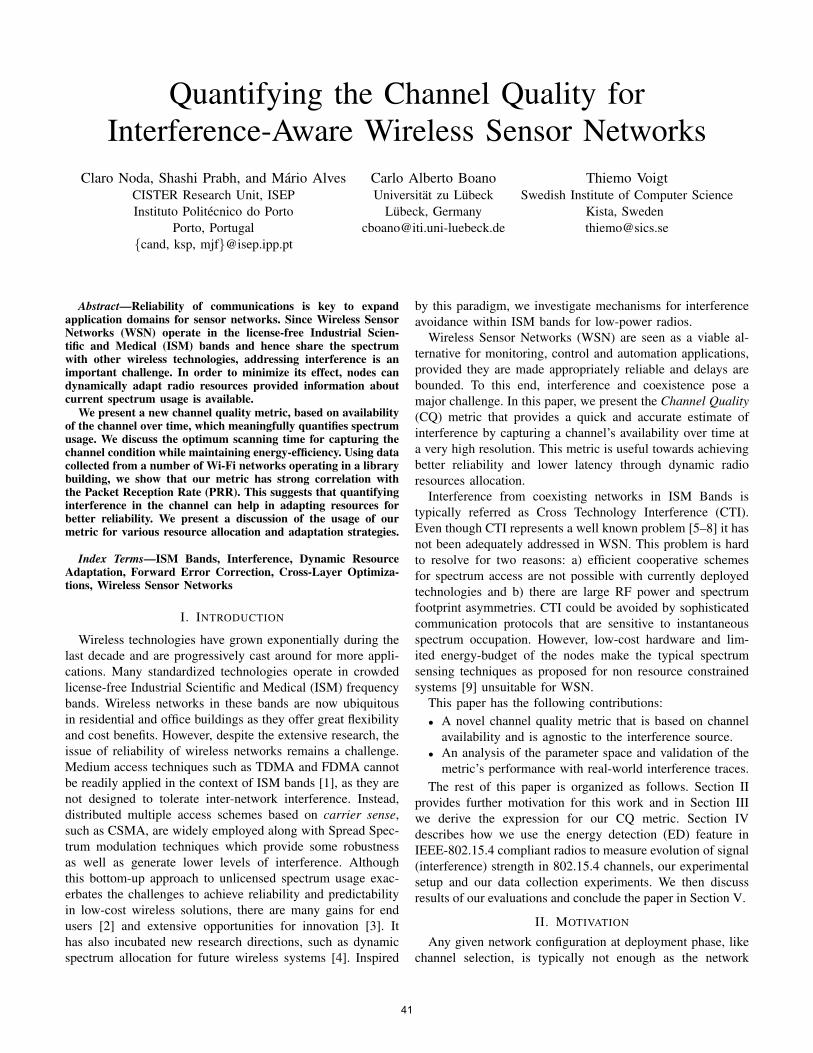
Quantifying the Channel Quality for

Interference-Aware Wireless Sensor Networks

Claro Noda, Shashi Prabh, and Mario Alves

CISTER Research Unit, ISEP

Instituto Politecnico do Porto

Porto, Portugal

{cand, ksp, mjf}@isep.ipp.pt

Carlo Alberto Boano

Universitat zu Lubeck

Lubeck, Germany

[email protected]

Thiemo Voigt

Swedish Institute of Computer Science

Kista, Sweden

[email protected]

Abstract—Reliability of communications is key to expandapplication domains for sensor networks. Since Wireless SensorNetworks (WSN) operate in the license-free Industrial Scien-tific and Medical (ISM) bands and hence share the spectrumwith other wireless technologies, addressing interference is animportant challenge. In order to minimize its effect, nodes candynamically adapt radio resources provided information aboutcurrent spectrum usage is available.

We present a new channel quality metric, based on availabilityof the channel over time, which meaningfully quantifies spectrumusage. We discuss the optimum scanning time for capturing thechannel condition while maintaining energy-efficiency. Using datacollected from a number of Wi-Fi networks operating in a librarybuilding, we show that our metric has strong correlation withthe Packet Reception Rate (PRR). This suggests that quantifyinginterference in the channel can help in adapting resources forbetter reliability. We present a discussion of the usage of ourmetric for various resource allocation and adaptation strategies.

Index Terms—ISM Bands, Interference, Dynamic ResourceAdaptation, Forward Error Correction, Cross-Layer Optimiza-tions, Wireless Sensor Networks

I. INTRODUCTION

Wireless technologies have grown exponentially during the

last decade and are progressively cast around for more appli-

cations. Many standardized technologies operate in crowded

license-free Industrial Scientific and Medical (ISM) frequency

bands. Wireless networks in these bands are now ubiquitous

in residential and office buildings as they offer great flexibility

and cost benefits. However, despite the extensive research, the

issue of reliability of wireless networks remains a challenge.

Medium access techniques such as TDMA and FDMA cannot

be readily applied in the context of ISM bands [1], as they are

not designed to tolerate inter-network interference. Instead,

distributed multiple access schemes based on carrier sense,

such as CSMA, are widely employed along with Spread Spec-

trum modulation techniques which provide some robustness

as well as generate lower levels of interference. Although

this bottom-up approach to unlicensed spectrum usage exac-

erbates the challenges to achieve reliability and predictability

in low-cost wireless solutions, there are many gains for end

users [2] and extensive opportunities for innovation [3]. It

has also incubated new research directions, such as dynamic

spectrum allocation for future wireless systems [4]. Inspired

by this paradigm, we investigate mechanisms for interference

avoidance within ISM bands for low-power radios.

Wireless Sensor Networks (WSN) are seen as a viable al-

ternative for monitoring, control and automation applications,

provided they are made appropriately reliable and delays are

bounded. To this end, interference and coexistence pose a

major challenge. In this paper, we present the Channel Quality

(CQ) metric that provides a quick and accurate estimate of

interference by capturing a channel’s availability over time at

a very high resolution. This metric is useful towards achieving

better reliability and lower latency through dynamic radio

resources allocation.

Interference from coexisting networks in ISM Bands is

typically referred as Cross Technology Interference (CTI).

Even though CTI represents a well known problem [5–8] it has

not been adequately addressed in WSN. This problem is hard

to resolve for two reasons: a) efficient cooperative schemes

for spectrum access are not possible with currently deployed

technologies and b) there are large RF power and spectrum

footprint asymmetries. CTI could be avoided by sophisticated

communication protocols that are sensitive to instantaneous

spectrum occupation. However, low-cost hardware and lim-

ited energy-budget of the nodes make the typical spectrum

sensing techniques as proposed for non resource constrained

systems [9] unsuitable for WSN.

This paper has the following contributions:

• A novel channel quality metric that is based on channel

availability and is agnostic to the interference source.

• An analysis of the parameter space and validation of the

metric’s performance with real-world interference traces.

The rest of this paper is organized as follows. Section II

provides further motivation for this work and in Section III

we derive the expression for our CQ metric. Section IV

describes how we use the energy detection (ED) feature in

IEEE-802.15.4 compliant radios to measure evolution of signal

(interference) strength in 802.15.4 channels, our experimental

setup and our data collection experiments. We then discuss

results of our evaluations and conclude the paper in Section V.

II. MOTIVATION

Any given network configuration at deployment phase, like

channel selection, is typically not enough as the network

41

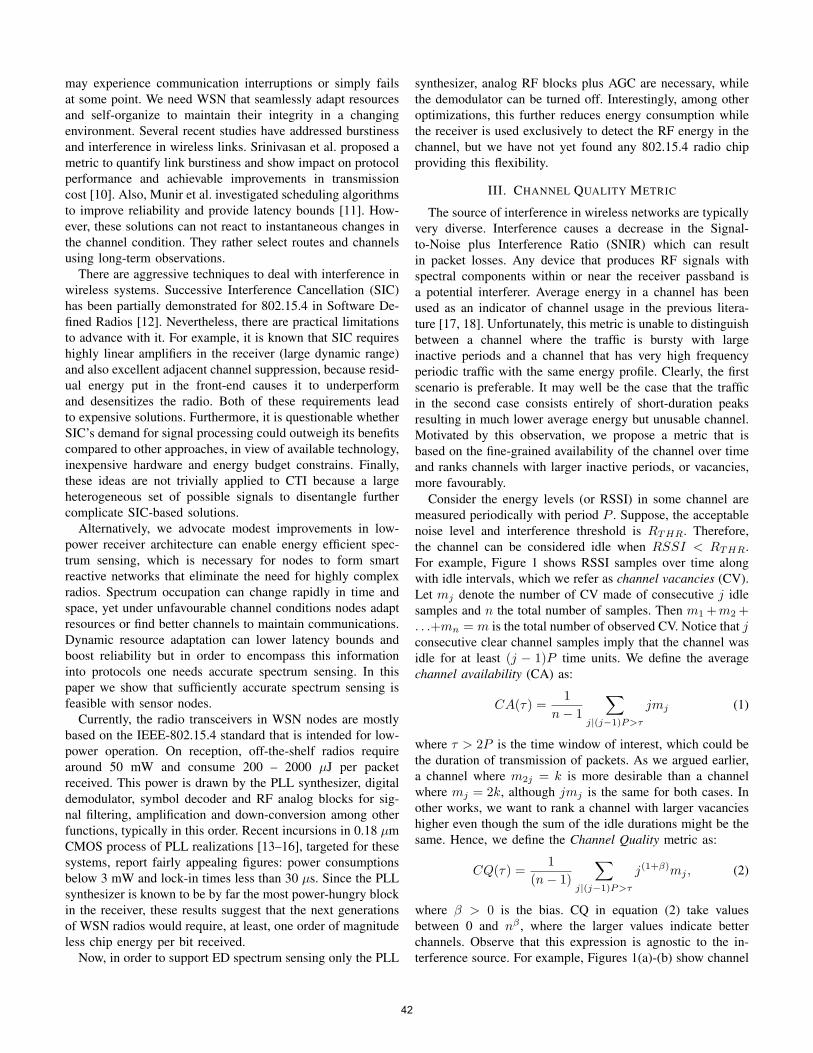
may experience communication interruptions or simply fails

at some point. We need WSN that seamlessly adapt resources

and self-organize to maintain their integrity in a changing

environment. Several recent studies have addressed burstiness

and interference in wireless links. Srinivasan et al. proposed a

metric to quantify link burstiness and show impact on protocol

performance and achievable improvements in transmission

cost [10]. Also, Munir et al. investigated scheduling algorithms

to improve reliability and provide latency bounds [11]. How-

ever, these solutions can not react to instantaneous changes in

the channel condition. They rather select routes and channels

using long-term observations.

There are aggressive techniques to deal with interference in

wireless systems. Successive Interference Cancellation (SIC)

has been partially demonstrated for 802.15.4 in Software De-

fined Radios [12]. Nevertheless, there are practical limitations

to advance with it. For example, it is known that SIC requires

highly linear amplifiers in the receiver (large dynamic range)

and also excellent adjacent channel suppression, because resid-

ual energy put in the front-end causes it to underperform

and desensitizes the radio. Both of these requirements lead

to expensive solutions. Furthermore, it is questionable whether

SIC’s demand for signal processing could outweigh its benefits

compared to other approaches, in view of available technology,

inexpensive hardware and energy budget constrains. Finally,

these ideas are not trivially applied to CTI because a large

heterogeneous set of possible signals to disentangle further

complicate SIC-based solutions.

Alternatively, we advocate modest improvements in low-

power receiver architecture can enable energy efficient spec-

trum sensing, which is necessary for nodes to form smart

reactive networks that eliminate the need for highly complex

radios. Spectrum occupation can change rapidly in time and

space, yet under unfavourable channel conditions nodes adapt

resources or find better channels to maintain communications.

Dynamic resource adaptation can lower latency bounds and

boost reliability but in order to encompass this information

into protocols one needs accurate spectrum sensing. In this

paper we show that sufficiently accurate spectrum sensing is

feasible with sensor nodes.

Currently, the radio transceivers in WSN nodes are mostly

based on the IEEE-802.15.4 standard that is intended for low-

power operation. On reception, off-the-shelf radios require

around 50 mW and consume 200 – 2000 µJ per packet

received. This power is drawn by the PLL synthesizer, digital

demodulator, symbol decoder and RF analog blocks for sig-

nal filtering, amplification and down-conversion among other

functions, typically in this order. Recent incursions in 0.18 µm

CMOS process of PLL realizations [13–16], targeted for these

systems, report fairly appealing figures: power consumptions

below 3 mW and lock-in times less than 30 µs. Since the PLL

synthesizer is known to be by far the most power-hungry block

in the receiver, these results suggest that the next generations

of WSN radios would require, at least, one order of magnitude

less chip energy per bit received.

Now, in order to support ED spectrum sensing only the PLL

synthesizer, analog RF blocks plus AGC are necessary, while

the demodulator can be turned off. Interestingly, among other

optimizations, this further reduces energy consumption while

the receiver is used exclusively to detect the RF energy in the

channel, but we have not yet found any 802.15.4 radio chip

providing this flexibility.

III. CHANNEL QUALITY METRIC

The source of interference in wireless networks are typically

very diverse. Interference causes a decrease in the Signal-

to-Noise plus Interference Ratio (SNIR) which can result

in packet losses. Any device that produces RF signals with

spectral components within or near the receiver passband is

a potential interferer. Average energy in a channel has been

used as an indicator of channel usage in the previous litera-

ture [17, 18]. Unfortunately, this metric is unable to distinguish

between a channel where the traffic is bursty with large

inactive periods and a channel that has very high frequency

periodic traffic with the same energy profile. Clearly, the first

scenario is preferable. It may well be the case that the traffic

in the second case consists entirely of short-duration peaks

resulting in much lower average energy but unusable channel.

Motivated by this observation, we propose a metric that is

based on the fine-grained availability of the channel over time

and ranks channels with larger inactive periods, or vacancies,

more favourably.

Consider the energy levels (or RSSI) in some channel are

measured periodically with period P . Suppose, the acceptable

noise level and interference threshold is RTHR. Therefore,

the channel can be considered idle when RSSI < RTHR.

For example, Figure 1 shows RSSI samples over time along

with idle intervals, which we refer as channel vacancies (CV).

Let mj denote the number of CV made of consecutive j idle

samples and n the total number of samples. Then m1+m2+. . .+mn = m is the total number of observed CV. Notice that j

consecutive clear channel samples imply that the channel was

idle for at least (j − 1)P time units. We define the average

channel availability (CA) as:

CA(τ) =1

n− 1

∑j|(j−1)P>τ

jmj (1)

where τ > 2P is the time window of interest, which could be

the duration of transmission of packets. As we argued earlier,

a channel where m2j = k is more desirable than a channel

where mj = 2k, although jmj is the same for both cases. In

other works, we want to rank a channel with larger vacancies

higher even though the sum of the idle durations might be the

same. Hence, we define the Channel Quality metric as:

CQ(τ) =1

(n− 1)

∑j|(j−1)P>τ

j(1+β)mj , (2)

where β > 0 is the bias. CQ in equation (2) take values

between 0 and nβ , where the larger values indicate better

channels. Observe that this expression is agnostic to the in-

terference source. For example, Figures 1(a)-(b) show channel

42

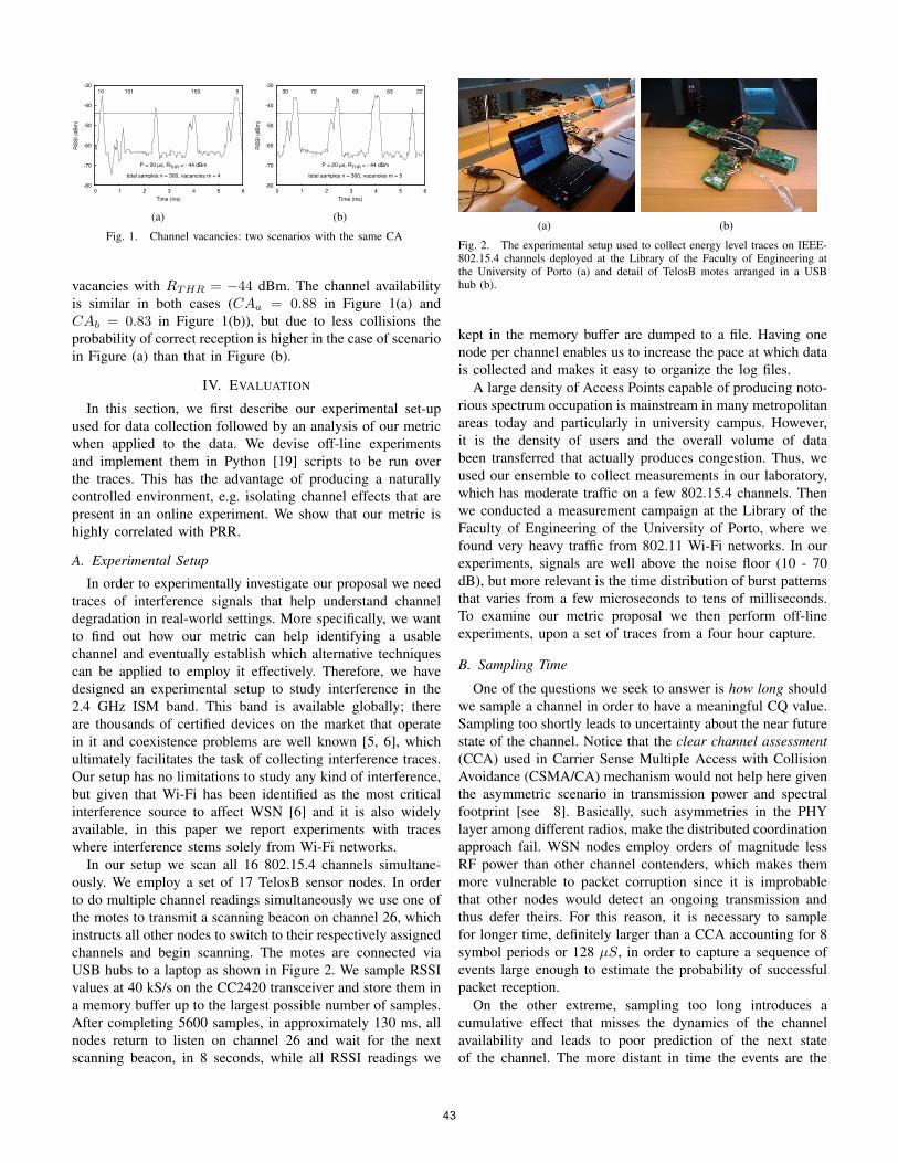
-80

-70

-60

-50

-40

-30

0 1 2 3 4 5 6

RS

SI

(dB

m)

Time (ms)

10 101 153 5

total samples n = 300, vacancies m = 4

P = 20 µs, RTHR = - 44 dBm

(a)

-80

-70

-60

-50

-40

-30

0 1 2 3 4 5 6

RS

SI

(dB

m)

Time (ms)

30 72 63 63 22

total samples n = 300, vacancies m = 5

P = 20 µs, RTHR = - 44 dBm

(b)

Fig. 1. Channel vacancies: two scenarios with the same CA

vacancies with RTHR = −44 dBm. The channel availability

is similar in both cases (CAa = 0.88 in Figure 1(a) and

CAb = 0.83 in Figure 1(b)), but due to less collisions the

probability of correct reception is higher in the case of scenario

in Figure (a) than that in Figure (b).

IV. EVALUATION

In this section, we first describe our experimental set-up

used for data collection followed by an analysis of our metric

when applied to the data. We devise off-line experiments

and implement them in Python [19] scripts to be run over

the traces. This has the advantage of producing a naturally

controlled environment, e.g. isolating channel effects that are

present in an online experiment. We show that our metric is

highly correlated with PRR.

A. Experimental Setup

In order to experimentally investigate our proposal we need

traces of interference signals that help understand channel

degradation in real-world settings. More specifically, we want

to find out how our metric can help identifying a usable

channel and eventually establish which alternative techniques

can be applied to employ it effectively. Therefore, we have

designed an experimental setup to study interference in the

2.4 GHz ISM band. This band is available globally; there

are thousands of certified devices on the market that operate

in it and coexistence problems are well known [5, 6], which

ultimately facilitates the task of collecting interference traces.

Our setup has no limitations to study any kind of interference,

but given that Wi-Fi has been identified as the most critical

interference source to affect WSN [6] and it is also widely

available, in this paper we report experiments with traces

where interference stems solely from Wi-Fi networks.

In our setup we scan all 16 802.15.4 channels simultane-

ously. We employ a set of 17 TelosB sensor nodes. In order

to do multiple channel readings simultaneously we use one of

the motes to transmit a scanning beacon on channel 26, which

instructs all other nodes to switch to their respectively assigned

channels and begin scanning. The motes are connected via

USB hubs to a laptop as shown in Figure 2. We sample RSSI

values at 40 kS/s on the CC2420 transceiver and store them in

a memory buffer up to the largest possible number of samples.

After completing 5600 samples, in approximately 130 ms, all

nodes return to listen on channel 26 and wait for the next

scanning beacon, in 8 seconds, while all RSSI readings we

(a) (b)

Fig. 2. The experimental setup used to collect energy level traces on IEEE-802.15.4 channels deployed at the Library of the Faculty of Engineering atthe University of Porto (a) and detail of TelosB motes arranged in a USBhub (b).

kept in the memory buffer are dumped to a file. Having one

node per channel enables us to increase the pace at which data

is collected and makes it easy to organize the log files.

A large density of Access Points capable of producing noto-

rious spectrum occupation is mainstream in many metropolitan

areas today and particularly in university campus. However,

it is the density of users and the overall volume of data

been transferred that actually produces congestion. Thus, we

used our ensemble to collect measurements in our laboratory,

which has moderate traffic on a few 802.15.4 channels. Then

we conducted a measurement campaign at the Library of the

Faculty of Engineering of the University of Porto, where we

found very heavy traffic from 802.11 Wi-Fi networks. In our

experiments, signals are well above the noise floor (10 - 70

dB), but more relevant is the time distribution of burst patterns

that varies from a few microseconds to tens of milliseconds.

To examine our metric proposal we then perform off-line

experiments, upon a set of traces from a four hour capture.

B. Sampling Time

One of the questions we seek to answer is how long should

we sample a channel in order to have a meaningful CQ value.

Sampling too shortly leads to uncertainty about the near future

state of the channel. Notice that the clear channel assessment

(CCA) used in Carrier Sense Multiple Access with Collision

Avoidance (CSMA/CA) mechanism would not help here given

the asymmetric scenario in transmission power and spectral

footprint [see 8]. Basically, such asymmetries in the PHY

layer among different radios, make the distributed coordination

approach fail. WSN nodes employ orders of magnitude less

RF power than other channel contenders, which makes them

more vulnerable to packet corruption since it is improbable

that other nodes would detect an ongoing transmission and

thus defer theirs. For this reason, it is necessary to sample

for longer time, definitely larger than a CCA accounting for 8

symbol periods or 128 µS, in order to capture a sequence of

events large enough to estimate the probability of successful

packet reception.

On the other extreme, sampling too long introduces a

cumulative effect that misses the dynamics of the channel

availability and leads to poor prediction of the next state

of the channel. The more distant in time the events are the

43

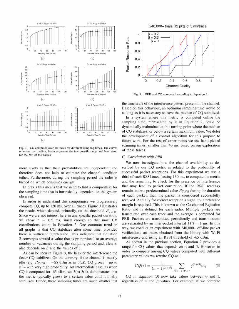
0

0.5

1

1.5

2

2.5

3

0 20 40 60 80 100 120

Ch

an

ne

l Q

ua

lity

Sampling Time, Ts (ms)

β = 0.2, RTHR = -55 dBm

(a)

0

0.5

1

1.5

2

2.5

3

0 20 40 60 80 100 120

Ch

an

ne

l Q

ua

lity


β = 0.2, RTHR = -65 dBm

(b)

0

2

4

6

8

10

12

14

16

0 20 40 60 80 100 120

Ch

an

ne

l Q

ua

lity


β = 0.5, RTHR = -65 dBm

(c)

0

50

100

150

200

250

0 20 40 60 80 100 120

Ch

an

ne

l Q

ua

lity


β = 1.0, RTHR = -65 dBm

(d)

0

0.5

1

1.5

2

2.5

3

0 20 40 60 80 100 120

Ch

an

ne

l Q

ua

lity


β = 0.2, RTHR = -75 dBm

(e)

0

2

4

6

8

10

12

14

16

0 20 40 60 80 100 120

Ch

an

ne

l Q

ua

lity


β = 0.5, RTHR = -75 dBm

(f)

Fig. 3. CQ computed over all traces for different sampling times. The curvesrepresent the median, boxes represent the interquartile range and bars standfor the rest of the values

more likely is that their probabilities are independent and

therefore does not help to estimate the channel condition

either. Furthermore, during the sampling period the radio is

turned on which consumes energy.

In praxis this means that we need to find a compromise for

the sampling time that is intrinsically dependent on the system

observed.

In order to understand this compromise we progressively

compute CQ, up to 120 ms, over all traces. Figure 3 illustrates

the results which depend, primarily, on the threshold RTHR.

Since we are not interest here in any specific packet duration,

we chose τ = 0.2 ms, small enough so that most CV

contributions count in Equation 2. One common trend in

all graphs is that CQ stabilizes after some time, provided

there is sufficient interference. This indicates that Equation

2 converges toward a value that is proportional to an average

number of vacancies during the sampling period and, clearly,

also depends on β and the values of j.

As can be seen in Figure 3, the heavier the interference the

faster CQ stabilizes. On the contrary, if the channel is mostly

idle (e.g. RTHR = −55 dBm as in 3(a)), CQ grows – up to

nβ– with very high probability. An intermediate case, as when

CQ is computed for -65 dBm, see 3(b)-3(d), demonstrates that

the metric typically grows to a certain value until it finally

stabilizes. Hence, these sampling times are much smaller that

0

0.2

0.4

0.6

0.8

1

0 0.2 0.4 0.6 0.8 1

Pa

cke

t R

ece

ptio

n R

ate

Channel Quality

240,000+ trials, 12 pkts of 5 ms/trace

β = 0.7β = 0.3

β = 0

Fig. 4. PRR and CQ computed according to Equation 3

the time scale of the interference pattern present in the channel.

Based on this behaviour, an optimum sampling time would be

as long as it is necessary to have the median of CQ stabilized.

In a system where this metric is computed online the

sampling time, represented by n in Equation 2, could be

dynamically maintained at this turning point where the median

of CQ stabilizes, or below a certain maximum value. We defer

the development of a control algorithm for this purpose to

future work. For the rest of experiments we use hand-picked

scanning times, smaller than 40 ms, based on our exploration

of these traces.

C. Correlation with PRR

We now investigate how the channel availability as de-

scribed by our CQ metric is related to the probability of

successful packet receptions. For this experiment we use a

third of each RSSI trace, lasting 130 ms, to compute the metric

and the remaining to check for the presence of interference

that may lead to packet corruption. If the RSSI readings

remain under a predetermined value RTHR during the duration

of each packet, then the packet is considered successfully

received. Actually for correct reception a signal to interference

margin is required. This is known as the Co-channel Rejection

Ratio and is defined for each radio. Multiple packets are

transmitted over each trace and the average is computed for

PRR. Packets are transmitted periodically and transmissions

are separated by an inter-packet interval IPI = 1 ms. In this

way, we conduct an experiment with 240,000+ off-line packet

verifications on traces obtained from the library with Wi-Fi

interference and using an RSSI threshold of -65 dBm.

As shown in the previous section, Equation 2 provides a

range for CQ values that depends on n and β. However, in

order to compare among CQ values computed with different

parameter values we rewrite CQ as:

CQ(τ) =1

(n− 1)(1+β)

∑j|(j−1)P>τ

j(1+β)mj , (3)

CQ in Equation (3) now take values between 0 and 1,

regardless of n and β values. For example, if we compute

44

Equation 3 with β = 0.3 for an 802.15.4 ACK frame lasting

352 µs, in the scenario in Figure 1(a) and (b) we obtain

CQa = 0.65 and CQb = 0.50, which are more accurately

reflect the difference among the two channels than previous

values from Equation 1.

Figure 4 shows the results where we find a strong correlation

with PRR. The curves correspond to the median and the error

bars represent the interquartile range computed over the entire

set of traces. We compute CQ for bias (β) values 0, 0.3 and 0.7

to highlight that β = 0.3 linearises the curves. Notice, β = 0is equivalent to average channel availability as described by

Equation 1. In this case CQ values grow faster than PRR which

indicates that despite channel been less occupied there are still

many collisions that hinder PRR values. As we increase β, this

selectively raises CQ favouring larger CV to have more weight

in the sum.

This is an interesting result, as been able to tune β and

maximize the correlation among PRR and CQ makes this

metric an accurate indicator of the channel condition. Similar

to the scanning time, an algorithm to find a value for β that

is optimum is left out of this paper.

D. Discussion

In this section we revisit some resource adaptation tech-

niques and discuss how they could be dynamically applied to

leverage our CQ metric for interference-aware communication

protocols.

Lin et al. demonstrated a novel pairwise transmission power

control for WSN that performs significantly better than node-

level or network-level power control methods [20]. They im-

prove PRR and energy consumption by dynamically adapting

the RF transmission power to maintain the minimum level

required to guarantee a good link. This is a clever approach

to compensate for the non-linear pathloss. However, it does

not account for two important aspects: a) the irreducible error

floor [21, Ch. 6] produced by fading can not be removed

by increasing transmission power and b) it does not address

external interference. A solution to both these problems is

dynamic frequency and power adaptation, simultaneously.

In this regard, one can augment such pairwise power control

mechanism with CQ, directly establishing a dynamic lower

bound for the RF power to use in the transmitter, previous

to actual transmissions. Besides, since maximum transmission

power can not be exceeded, an alternative such as a moving

to a different channel may be inferred immediately. Starting

from the RSSI samples in memory, we could ask the question:

which signal level would result in a CQ value that satisfies

a given requirement for channel usage under the current

interference level?

In general, protocols designed for multichannel operation

can maintain good links using a channel ranking with dis-

tributed CQ computations, among neighbour nodes, provided

a control channel among them is stable. Additionally, this

could aid topology changes when interferers spectral footprint

is very large, as in 802.11n, to take advantage of the irregular

coverage, common in some indoor environments.

Successful transmissions in the scenarios in Figure 1 also

depend on the packet size. Certain packet size would maximize

throughput or minimize the time to deliver a data object

over the channel, for a given interference level. Observe that

shorter packets have better chances of avoiding collisions (and

hence retransmissions) but also result in higher overhead due

to fixed packet headers and acknowledgement delays. One

could look into the relationship between these optimum packet

sizes and the CQ values computed on the channel. Similar

to the PRR correlation in Figure 4, there would be a value

of β that linearises such dependency. Based on observed CQ

values protocols can then tune packet size to transfer data in

a minimum time.

FEC techniques pose a trade-off between data recovery

capacity and its inherent payload and computation overhead.

Recently, Liang et al. demonstrated the Reed-Solomon (RS)

correcting codes performs well while recovering packets af-

fected by 802.11 interfering signals [8]. Since interference

levels may vary extensively it is interesting to see if this

solution can benefit from simple CQ based optimizations.

On the other hand, energy cost to compute the CQ metric

must be further explored in view of overall energy balance

in dynamic resource adaptation. In future work we plan to

extend our experiments and later implement the metric on

WSN hardware.

V. CONCLUSIONS

We introduced a new channel quality metric that is based

on the availability of the channel over time. The metric is

useful for interference aware protocols in WSN. We described

our experimental setup for collecting real-world interference

traces in the 2.4 GHz ISM band. Using this data, we showed

that our metric has strong correlation with PRR. Thus, our

metric’s characterization of a channel is reliable and applicable

in practice. We also discussed dynamic resource allocation

techniques for interference-aware protocols in WSN for which

our metric can prove to be useful. We are currently working

on a software implementation of CQ for WSN hardware to

further validate its performance in online experiments.

REFERENCES

[1] Kenneth R. Carter. Unlicensed to kill: a brief history of

the Part 15 rules. Info, 11(5):8–18, 2009. ISSN 1463-

6697.

[2] Henry Goldberg. Grazing on the commons: the emer-

gence of Part 15. Info - The journal of policy, regulation

and strategy for telecommunications, 11(5):72–75, 2009.

ISSN 1463-6697.

[3] Vic Hayes and Wolter Lemstra. Licence-exempt: the

emergence of Wi-Fi. Info - The journal of policy,

regulation and strategy for telecommunications, 11(5):

57–71, 2009. ISSN 1463-6697.

[4] Ian F. Akyildiz, Won-Yeol Lee, Mehmet C. Vuran, and

Shantidev Mohanty. Next generation/dynamic spectrum

45

access/cognitive radio wireless networks: A survey. Com-

puter Networks, 50(13):2127 – 2159, 2006. ISSN 1389-

1286.

[5] A. Sikora and V. Groza. Coexistence of IEEE 802.15.4

with other systems in the 2.4 GHz-ISM-Band. In IEEE

Instrumentation and Measurement Technology, pages

1786–1791, Ottawa, Canada, May 2005.

[6] M. Petrova, L. Wu, P. Mahonen, and J. Riihijarvi. In-

terference Measurements on Performance Degradation

between Colocated IEEE 802.11g/n and IEEE 802.15.4

Networks. In International Conference on Networking

(ICN), Sainte-Luce, Martinique, April 2007. ISBN 0-

7695-2805-8.

[7] Jan-Hinrich Hauer, Andreas Willig, and Adam Wolisz.

Mitigating the Effects of RF Interference through RSSI-

Based Error Recovery. In Jorge Silva, Bhaskar Krishna-

machari, and Fernando Boavida, editors, Wireless Sensor

Networks, volume 5970 of Lecture Notes in Computer

Science, chapter 15, pages 224–239. Springer Berlin /

Heidelberg, Berlin, Heidelberg, 2010. ISBN 978-3-642-

11916-3.

[8] Chieh-Jan Mike Liang, Bodhi Priyantha, Jie Liu, and

Andreas Terzis. Surviving Wi-Fi Interference in low-

power ZigBee Networks. In Proceedings of the 8th

ACM Conference on Embedded Networked Sensor Sys-

tems (SenSys’10), pages 309–322, Zurich, Switzerland,

November 2010.

[9] T. Yucek and H. Arslan. A Survey of Spectrum Sensing

Algorithms for Cognitive Radio Applications. IEEE

Communications Surveys Tutorials, 11(1), 2009.

[10] Kannan Srinivasan, Maria A. Kazandjieva, Saatvik Agar-

wal, and Philip Levis. The beta-factor: measuring wire-

less link burstiness. In SenSys, pages 29–42, 2008.

[11] Sirajum Munir, Shan Lin, Enamul Hoque, S. M. Shahriar

Nirjon, John A. Stankovic, and Kamin Whitehouse. Ad-

dressing Burstiness for Reliable Communication and La-

tency Bound Generation in Wireless Sensor Networks. In

ACM/IEEE IPSN, pages 303–314, Stockholm, Sweden,

April 2010.

[12] Daniel Halperin, Thomas Anderson, and David Wether-

all. Taking the sting out of carrier sense: interference

cancellation for wireless LANs. In Proceedings of the

14th ACM international conference on Mobile computing

and networking, MobiCom ’08, pages 339–350, New

York, NY, USA, 2008. ACM. ISBN 978-1-60558-096-8.

[13] M. Vamshi Krishna, J. Xie, W.M. Lim, M.A. Do, K.S.

Yeo, and C.C. Boon. A low power fully programmable

1MHz resolution 2.4GHz CMOS PLL frequency synthe-

sizer. In Biomedical Circuits and Systems Conference,

2007. BIOCAS 2007. IEEE, pages 187 –190, 2007.

[14] Louis-Francois Tanguay and Mohamad Sawan. An ultra-

low power ISM-band integer-n frequency synthesizer

dedicated to implantable medical microsystems. Ana-

log Integr. Circuits Signal Process., 58:205–214, March

2009. ISSN 0925-1030.

[15] Wu Xiushan, Wang Zhigong, Li Zhiqun, Xia Jun, and

Li Qing. Design and realization of an ultra-low-power

low-phase-noise CMOS LC-VCO. Journal of Semicon-

ductors, 31(8):085007, 2010.

[16] Geng Zhiqing, Yan Xiaozhou, Lou Wenfeng, Feng Peng,

and Wu Nanjian. A low power fast-settling frequency-

presetting PLL frequency synthesizer. Journal of Semi-

conductors, 31(8):085002, 2010.

[17] Federico Penna, Claudio Pastrone, Maurizio A. Spirito,

and Roberto Garello. Measurement-Based Analysis of

Spectrum Sensing in Adaptive WSNs under Wi-Fi and

Bluetooth Interference. In VTC Spring. IEEE, 2009.

[18] Luca Stabellini and Jens Zander. Energy-efficient De-

tection of Intermittent Interference in Wireless Sensor

Networks. Int. J. Sen. Netw., 8:27–40, July 2010. ISSN

1748-1279.

[19] Guido Van Rossum. Python for Unix/C Programmers.

In Proc. of the NLUUG najaarsconferentie. Dutch UNIX

users group, 1993.

[20] Shan Lin, Jingbin Zhang, Gang Zhou, Lin Gu, John A.

Stankovic, and Tian He. ATPC: adaptive transmission

power control for wireless sensor networks. In Andrew T.

Campbell, Philippe Bonnet, and John S. Heidemann,

editors, SenSys, pages 223–236. ACM, 2006. ISBN 1-

59593-343-3.

[21] Andrea Goldsmith. Wireless Communications. Cam-

bridge University Press, New York, NY, USA, 2005.

ISBN 0521837162.

46

Existing offset assignments are near optimal for an industrial AFDX network

Xiaoting Li, Jean-Luc Scharbarg, Christian FraboulINP-ENSEEIHT IRIT, Universite de Toulouse

Toulouse, France{Xiaoting.Li, Jean-Luc.Scharbarg, Christian.Fraboul}@enseeiht.fr

Frederic RidouardLISI-ENSMA, University of Poitiers

Poitiers, [email protected]

Abstract—Avionics Full DupleX Switched Ethernet (AFDX)has been developed for modern aircraft such as Airbus 380. Dueto the non-determinism of switching mechanism, a worst-casedelay analysis of the flows entering the network is a key issuefor certification reasons. Up to now most existing approaches(such as Network Calculus) consider that all the flows areasynchronous and they do not take into account the schedulingof flows generated by the same end system. It is then pessimisticto take into account such a synchronous scenario. Each endsystem can be considered as an offset free system, thus themain objective of this paper is to evaluate existing offsetassignments in the context of an industrial AFDX network.Existing offset assignments are adapted to take into accountspecific characteristics of an AFDX network. Worst-case delayresults are obtained according to these offset heuristics. It isshown that some existing heuristics are not efficient while someare near optimal for the studied industrial AFDX network.

Keywords-AFDX network, offset assignment, worst-case de-lay

I. I NTRODUCTION

Avionic Full DupleX Switched Ethernet (AFDX [1]) hasbeen proposed in order to satisfy the growing requirementsof avionics application. Such a network is defined based onstatic network configuration and routing. The demonstrationof a determined upper bound for end-to-end (ETE) commu-nication delays on such a real-time network plays a key role.Different methods [2]–[5] have been presented for the worst-case delay analysis on the AFDX network. Among them, theNetwork Calculus [6] has been used for the certification ofAirbus 380.

Since each end system of the AFDX network schedulesits flows according to a local clock, it is pessimistic toconsider that all frames arrive simultaneously (synchronousscenario) on this network. This issue has been addressed in[7], in which a computation method integrating the offsetsof flows based on the Network Calculus approach has beendeveloped. However, only one offset assignment originallydesigned for the CAN network in [8] was applied to anindustrial AFDX network. It is interesting to consider otherexisting offset assignments [9], [10] in order to find the bestalgorithm for an industrial AFDX network. Moreover, theexisting algorithms can be adapted in order to take intoaccount specific characteristics of an AFDX network.

The objective of this paper is to evaluate and com-pute offset assignment algorithms for an industrial AFDXnetwork. The goal of the evaluation is to measure thegap between offset assignment based on heuristics and theoptimal assignment, which is intractable on an industrialAFDX network. An upper bound on this gap is computed,based on an optimal scenario.

This paper is organized as follows. Section II shortly in-troduces the context of the studied industrial AFDX networkand existing offset assignments. Section III derives an idealoffset assignment which gives an optimal scenario for thescheduled flows. In Section IV, new heuristics integratingthe AFDX characteristics are proposed. The existing andproposed offset assignments are applied to the industrialAFDX network, and their results are compared and analyzedin Section V. Section VI concludes and indicates directionsfor future research.

II. CONTEXT

A. Introduction of the industrial AFDX network

An AFDX network [1] is composed of end systemsand switches. The inputs and outputs of the AFDX net-work, calledend systems (ES), are connected by severalinterconnected AFDX switches. Each end system can beconnected to only one port of an AFDX switch and each portof an AFDX switch can be connected at most to one endsystem. Links between switches work in full-duplex mode.

A V irtual Link (V L) standardized by ARINC-664 is aconcept of virtual communication channel, which staticallydefines the flows. A connection defined by a Virtual Linkis unidirectional, including one source end system and oneor more paths leading to different destination end systems(multicast nature). A VL is characterized by:

• Bandwidth Allocation Gap (BAG), the minimumdelay between two consecutive frames of correspondingVL ranging in powers of 2 from1 ms to 128 ms, and

• Smin and Smax, the minimum and maximum framelength which respect the standard Ethernet frame.

An AFDX network architecture is illustrated by Figure 1.According to this architecture, there are five end systems andtwo AFDX switches. On the example,v1 has a unique path{e1 −S1 −S2 − e4} andv5 has multi-paths{e3 − S2 − e4}and{e3 − S2 − e5}.

47

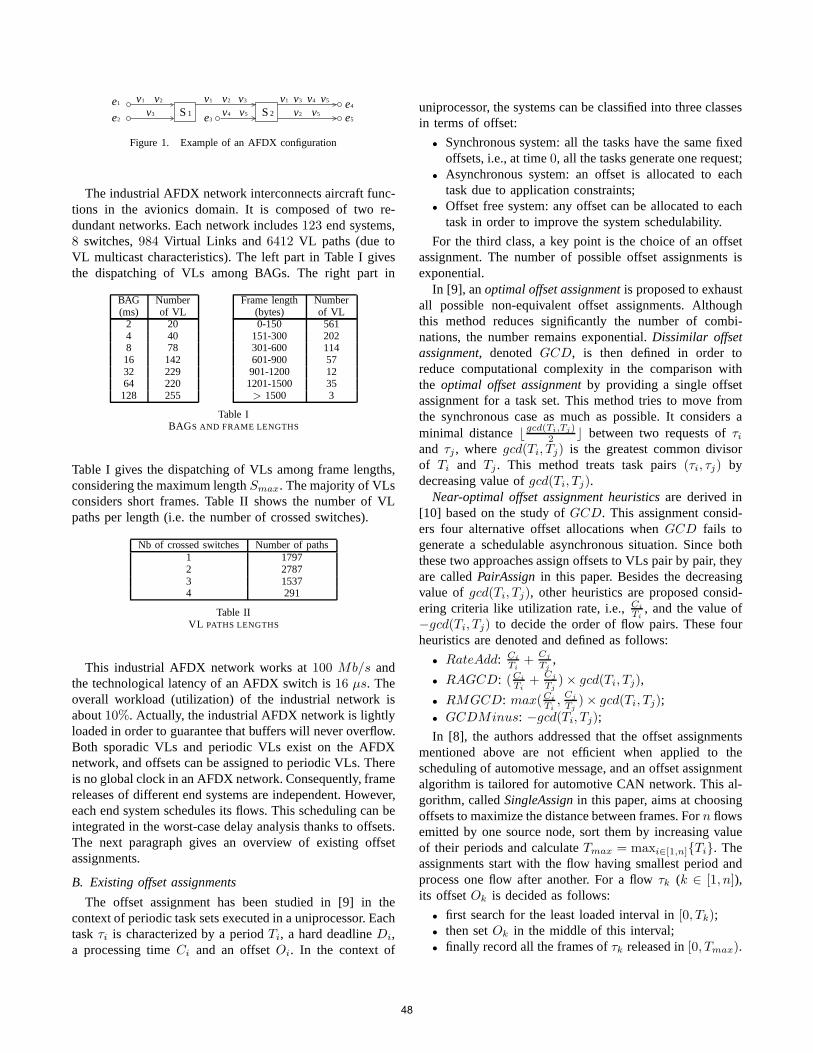
S1

1v 2v 3vS24v 5v

2v1v3v

e1

e2 e3

4v 5v1v 3v e4

e55v2v

Figure 1. Example of an AFDX configuration

The industrial AFDX network interconnects aircraft func-tions in the avionics domain. It is composed of two re-dundant networks. Each network includes123 end systems,8 switches,984 Virtual Links and6412 VL paths (due toVL multicast characteristics). The left part in Table I givesthe dispatching of VLs among BAGs. The right part in

BAG Number Frame length Number(ms) of VL (bytes) of VL

2 20 0-150 5614 40 151-300 2028 78 301-600 11416 142 601-900 5732 229 901-1200 1264 220 1201-1500 35128 255 > 1500 3

Table IBAGS AND FRAME LENGTHS

Table I gives the dispatching of VLs among frame lengths,considering the maximum lengthSmax. The majority of VLsconsiders short frames. Table II shows the number of VLpaths per length (i.e. the number of crossed switches).

Nb of crossed switches Number of paths1 17972 27873 15374 291

Table IIVL PATHS LENGTHS

This industrial AFDX network works at100 Mb/s andthe technological latency of an AFDX switch is16 µs. Theoverall workload (utilization) of the industrial network isabout10%. Actually, the industrial AFDX network is lightlyloaded in order to guarantee that buffers will never overflow.Both sporadic VLs and periodic VLs exist on the AFDXnetwork, and offsets can be assigned to periodic VLs. Thereis no global clock in an AFDX network. Consequently, framereleases of different end systems are independent. However,each end system schedules its flows. This scheduling can beintegrated in the worst-case delay analysis thanks to offsets.The next paragraph gives an overview of existing offsetassignments.

B. Existing offset assignments

The offset assignment has been studied in [9] in thecontext of periodic task sets executed in a uniprocessor. Eachtask τi is characterized by a periodTi, a hard deadlineDi,a processing timeCi and an offsetOi. In the context of

uniprocessor, the systems can be classified into three classesin terms of offset:

• Synchronous system: all the tasks have the same fixedoffsets, i.e., at time0, all the tasks generate one request;

• Asynchronous system: an offset is allocated to eachtask due to application constraints;

• Offset free system: any offset can be allocated to eachtask in order to improve the system schedulability.

For the third class, a key point is the choice of an offsetassignment. The number of possible offset assignments isexponential.

In [9], anoptimal offset assignmentis proposed to exhaustall possible non-equivalent offset assignments. Althoughthis method reduces significantly the number of combi-nations, the number remains exponential.Dissimilar offsetassignment, denotedGCD, is then defined in order toreduce computational complexity in the comparison withthe optimal offset assignmentby providing a single offsetassignment for a task set. This method tries to move fromthe synchronous case as much as possible. It considers aminimal distance⌊ gcd(Ti,Tj)

2 ⌋ between two requests ofτiand τj , wheregcd(Ti, Tj) is the greatest common divisorof Ti and Tj . This method treats task pairs(τi, τj) bydecreasing value ofgcd(Ti, Tj).

Near-optimal offset assignment heuristicsare derived in[10] based on the study ofGCD. This assignment consid-ers four alternative offset allocations whenGCD fails togenerate a schedulable asynchronous situation. Since boththese two approaches assign offsets to VLs pair by pair, theyare calledPairAssign in this paper. Besides the decreasingvalue of gcd(Ti, Tj), other heuristics are proposed consid-ering criteria like utilization rate, i.e.,Ci

Ti, and the value of

−gcd(Ti, Tj) to decide the order of flow pairs. These fourheuristics are denoted and defined as follows:

• RateAdd: Ci

Ti+

Cj

Tj,

• RAGCD: (Ci

Ti+

Cj

Tj)× gcd(Ti, Tj),

• RMGCD: max(Ci

Ti,Cj

Tj)× gcd(Ti, Tj);

• GCDMinus: −gcd(Ti, Tj);

In [8], the authors addressed that the offset assignmentsmentioned above are not efficient when applied to thescheduling of automotive message, and an offset assignmentalgorithm is tailored for automotive CAN network. This al-gorithm, calledSingleAssignin this paper, aims at choosingoffsets to maximize the distance between frames. Forn flowsemitted by one source node, sort them by increasing valueof their periods and calculateTmax = maxi∈[1,n]{Ti}. Theassignments start with the flow having smallest period andprocess one flow after another. For a flowτk (k ∈ [1, n]),its offsetOk is decided as follows:

• first search for the least loaded interval in[0, Tk);• then setOk in the middle of this interval;• finally record all the frames ofτk released in[0, Tmax).

48

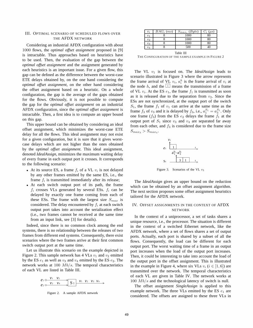
III. O PTIMAL SCENARIO OF SCHEDULED FLOWS OVER

THE AFDX NETWORK

Considering an industrial AFDX configuration with about1000 flows, theoptimal offset assignmentproposed in [9]is intractable. Thus approaches based on heuristics haveto be used. Then, the evaluation of the gap between theoptimal offset assignmentand the assignment generated byeach heuristics is an important issue. For a given flow, thisgap can be defined as the difference between the worst-caseETE delays obtained by, on the one hand considering theoptimal offset assignment, on the other hand consideringthe offset assignment based on a heuristic. On a wholeconfiguration, the gap is the average of the gaps obtainedfor the flows. Obviously, it is not possible to computethe gap for theoptimal offset assignmenton an industrialAFDX configuration, since theoptimal offset assignmentisintractable. Then, a first idea is to compute an upper boundon this gap.

This upper bound can be obtained by considering an idealoffset assignment, which minimizes the worst-case ETEdelay for all the flows. This ideal assignment may not existfor a given configuration, but it is sure that it gives worst-case delays which are not higher than the ones obtainedby the optimal offset assignment. This ideal assignment,denotedIdealAssign, minimizes the maximum waiting delayof every frame in each output port it crosses. It correspondsto the following scenario:

• At its source ES, a framefi of a VL vi is not delayedby any other frames emitted by the same ES, i.e., theframefi is transmitted immediately after its release;

• At each switch output port of its path, the framefi crosses VLs generated by several ESs.fi can bedelayed by exactly one frame coming from each ofthese ESs. The frame with the largest sizeSmax isconsidered. The delay encountered byfi at each switchoutput port takes into account the serialization effect(i.e., two frames cannot be received at the same timefrom an input link, see [3] for details).

Indeed, since there is no common clock among the endsystems, there is no relationship between the releases of twoframes from different end systems. Consequently, there existscenarios where the two frames arrive at their first commonswitch output port at the same time.

Let us illustrate this scenario on the example depicted inFigure 2. This sample network has 4 VLsv1 andv2 emittedby the ESe1 as well asv3 andv4 emitted by the ESe2. Thenetwork works at100 Mb/s. The temporal characteristicsof each VL are listed in Table III.

S1

1v3v

2v4v

e1

e2

3v1v 2v 4v

Figure 2. A sample AFDX network

vi BAGi (ms) Smaxi(Byte) Ci (µs)

v1 8 1000 80v2 8 1000 80v3 8 1000 80v4 8 500 40

Table IIITHE CONFIGURATION OF THE SAMPLE EXAMPLE INFIGURE 2

The VL v1 is focused on. TheIdealAssign leads toscenario illustrated in Figure 3 where the arrow representsthe frame arrival of VLvi, ahi is the frame arrival ofvi atthe nodeh, and the i means the transmission of a frameof VL vi. At the ESe1, the framef1 is transmitted as soonas it is released due to the separation fromv2. Since theESs are not synchronized, at the output port of the switchS1, the framef1 of v1 can arrive at the same time as theframef3 of v3 and it is delayed byf3, i.e.,aS1

1 = aS1

3 . Onlyone frame (f3) from the ESe2 delays the framef1 at theoutput port ofS1 sincev3 and v4 are separated far awayfrom each other, andf3 is considered due to the frame sizeSmax3

> Smax4.

v1

1e

S1

S1S1

3 1

1

=aa1 3

t

t

Figure 3. Scenarios of the VLv1

The IdealAssigngives an upper bound on the reductionwhich can be obtained by an offset assignment algorithm.The next section proposes some offset assignment heuristicstailored for the AFDX network.

IV. OFFSET ASSIGNMENTS IN THE CONTEXT OFAFDXNETWORK

In the context of a uniprocessor, a set of tasks shares aunique resource, i.e., the processor. The situation is differentin the context of a switched Ethernet network, like theAFDX network, where a set of flows shares a set of outputports. Actually, each port is shared by a subset of all theflows. Consequently, the load can be different for eachoutput port. The worst waiting time of a frame in an outputport increases when the load of the output port increases.Then, it could be interesting to take into account the load ofthe output port in the offset assignment. This is illustratedin the example in Figure 4, where six VLsvi (i ∈ [1, 6]) aretransmitted over the network. The temporal characteristicsof each VL are given in Table IV. The network works at100 Mb/s and the technological latency of switch is null.

The offset assignmentSingleAssignis applied to thisexample network. The three VLs emitted by the ESe1 areconsidered. The offsets are assigned to these three VLs in

49

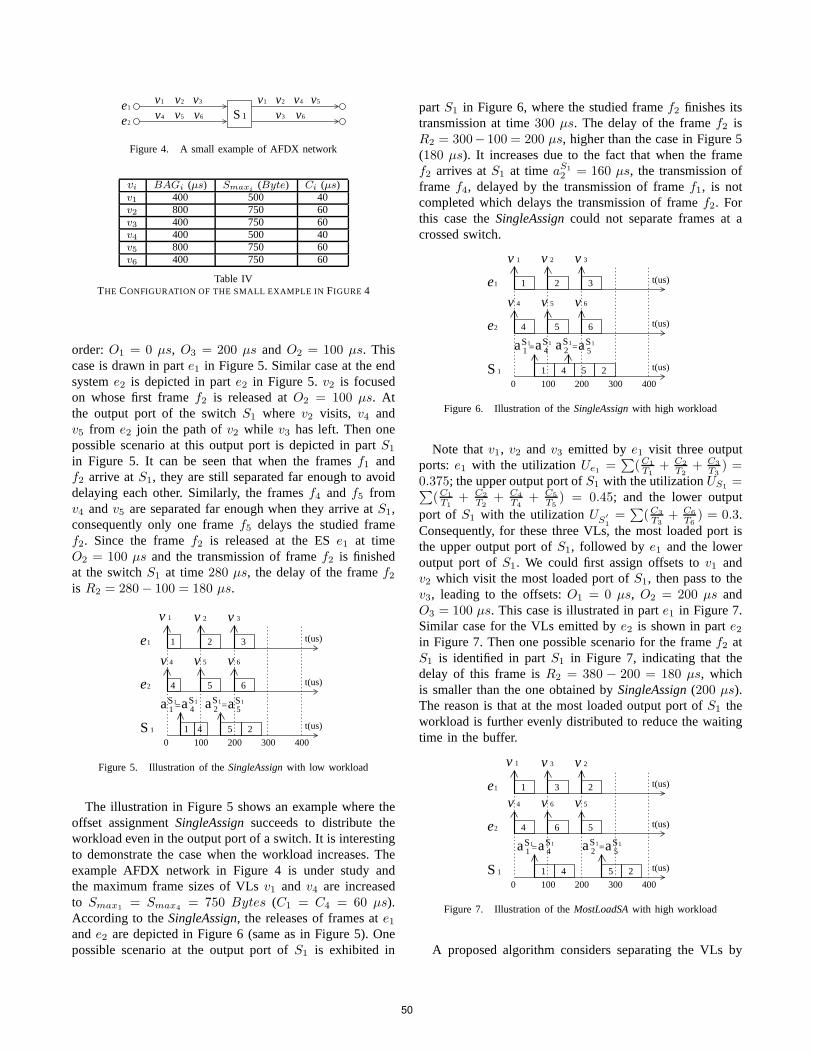
S1

v1e1

e2

v3v2 v5v4v2v1

v4 v5 v6 v6v3

Figure 4. A small example of AFDX network

vi BAGi (µs) Smaxi(Byte) Ci (µs)

v1 400 500 40v2 800 750 60v3 400 750 60v4 400 500 40v5 800 750 60v6 400 750 60

Table IVTHE CONFIGURATION OF THE SMALL EXAMPLE IN FIGURE 4

order:O1 = 0 µs, O3 = 200 µs andO2 = 100 µs. Thiscase is drawn in parte1 in Figure 5. Similar case at the endsysteme2 is depicted in parte2 in Figure 5.v2 is focusedon whose first framef2 is released atO2 = 100 µs. Atthe output port of the switchS1 where v2 visits, v4 andv5 from e2 join the path ofv2 while v3 has left. Then onepossible scenario at this output port is depicted in partS1

in Figure 5. It can be seen that when the framesf1 andf2 arrive atS1, they are still separated far enough to avoiddelaying each other. Similarly, the framesf4 and f5 fromv4 andv5 are separated far enough when they arrive atS1,consequently only one framef5 delays the studied framef2. Since the framef2 is released at the ESe1 at timeO2 = 100 µs and the transmission of framef2 is finishedat the switchS1 at time280 µs, the delay of the framef2is R2 = 280− 100 = 180 µs.

S1

aS12 aS1

5=aS11 aS1

4=

v 4

e2

v 6v 5

t(us)4 5 6

v 1

e1

v 2 v 3

t(us)1 2 3

4003002001000

t(us)1 4 5 2

Figure 5. Illustration of theSingleAssignwith low workload

The illustration in Figure 5 shows an example where theoffset assignmentSingleAssignsucceeds to distribute theworkload even in the output port of a switch. It is interestingto demonstrate the case when the workload increases. Theexample AFDX network in Figure 4 is under study andthe maximum frame sizes of VLsv1 and v4 are increasedto Smax1

= Smax4= 750 Bytes (C1 = C4 = 60 µs).

According to theSingleAssign, the releases of frames ate1ande2 are depicted in Figure 6 (same as in Figure 5). Onepossible scenario at the output port ofS1 is exhibited in

partS1 in Figure 6, where the studied framef2 finishes itstransmission at time300 µs. The delay of the framef2 isR2 = 300− 100 = 200 µs, higher than the case in Figure 5(180 µs). It increases due to the fact that when the framef2 arrives atS1 at timeaS1

2 = 160 µs, the transmission offrame f4, delayed by the transmission of framef1, is notcompleted which delays the transmission of framef2. Forthis case theSingleAssigncould not separate frames at acrossed switch.

S1

aS12 aS1

5=aS11 aS1

4=

e1

v 2 v 3

v 4

e2

v 5 v 6

v 1

4003002001000

1 4 5 2 t(us)

1 2 3 t(us)

5 64 t(us)

Figure 6. Illustration of theSingleAssignwith high workload

Note thatv1, v2 and v3 emitted bye1 visit three outputports: e1 with the utilizationUe1 =

∑(C1

T1

+ C2

T2

+ C3

T3

) =0.375; the upper output port ofS1 with the utilizationUS1

=∑(C1

T1+ C2

T2+ C4

T4+ C5

T5) = 0.45; and the lower output

port of S1 with the utilizationUS

′

1

=∑

(C3

T3

+ C6

T6

) = 0.3.Consequently, for these three VLs, the most loaded port isthe upper output port ofS1, followed by e1 and the loweroutput port ofS1. We could first assign offsets tov1 andv2 which visit the most loaded port ofS1, then pass to thev3, leading to the offsets:O1 = 0 µs, O2 = 200 µs andO3 = 100 µs. This case is illustrated in parte1 in Figure 7.Similar case for the VLs emitted bye2 is shown in parte2in Figure 7. Then one possible scenario for the framef2 atS1 is identified in partS1 in Figure 7, indicating that thedelay of this frame isR2 = 380 − 200 = 180 µs, whichis smaller than the one obtained bySingleAssign(200 µs).The reason is that at the most loaded output port ofS1 theworkload is further evenly distributed to reduce the waitingtime in the buffer.

S1

aS11 aS1

4= aS12 aS1

5=

v 4

e2

v 5v 6

6 54 t(us)

v 1

e1

v 3 v 2

1 23 t(us)

4003002001000

1 4 t(us)25

Figure 7. Illustration of theMostLoadSAwith high workload

A proposed algorithm considers separating the VLs by

50

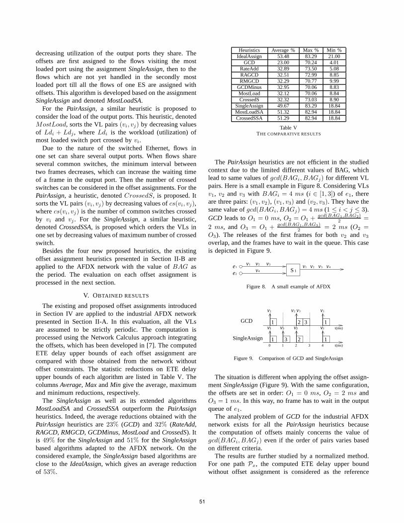
decreasing utilization of the output ports they share. Theoffsets are first assigned to the flows visiting the mostloaded port using the assignmentSingleAssign, then to theflows which are not yet handled in the secondly mostloaded port till all the flows of one ES are assigned withoffsets. This algorithm is developed based on the assignmentSingleAssignand denotedMostLoadSA.

For the PairAssign, a similar heuristic is proposed toconsider the load of the output ports. This heuristic, denotedMostLoad, sorts the VL pairs(vi, vj) by decreasing valuesof Ldi + Ldj , whereLdi is the workload (utilization) ofmost loaded switch port crossed byvi.

Due to the nature of the switched Ethernet, flows inone set can share several output ports. When flows shareseveral common switches, the minimum interval betweentwo frames decreases, which can increase the waiting timeof a frame in the output port. Then the number of crossedswitches can be considered in the offset assignments. For thePairAssign, a heuristic, denotedCrossedS, is proposed. Itsorts the VL pairs(vi, vj) by decreasing values ofcs(vi, vj),wherecs(vi, vj) is the number of common switches crossedby vi and vj . For the SingleAssign, a similar heuristic,denotedCrossedSSA, is proposed which orders the VLs inone set by decreasing values of maximum number of crossedswitch.

Besides the four new proposed heuristics, the existingoffset assignment heuristics presented in Section II-B areapplied to the AFDX network with the value ofBAG asthe period. The evaluation on each offset assignment isprocessed in the next section.

V. OBTAINED RESULTS

The existing and proposed offset assignments introducedin Section IV are applied to the industrial AFDX networkpresented in Section II-A. In this evaluation, all the VLsare assumed to be strictly periodic. The computation isprocessed using the Network Calculus approach integratingthe offsets, which has been developed in [7]. The computedETE delay upper bounds of each offset assignment arecompared with those obtained from the network withoutoffset constraints. The statistic reductions on ETE delayupper bounds of each algorithm are listed in Table V. ThecolumnsAverage, Max andMin give the average, maximumand minimum reductions, respectively.

The SingleAssignas well as its extended algorithmsMostLoadSAand CrossedSSAoutperform thePairAssignheuristics. Indeed, the average reductions obtained with thePairAssignheuristics are23% (GCD) and 32% (RateAdd,RAGCD, RMGCD, GCDMinus, MostLoadandCrossedS). Itis 49% for the SingleAssignand 51% for the SingleAssignbased algorithms adapted to the AFDX network. On theconsidered example, theSingleAssignbased algorithms areclose to theIdealAssign, which gives an average reductionof 53%.

Heuristics Average % Max % Min %IdealAssign 53.48 83.29 21.00

GCD 23.00 70.24 4.01RateAdd 32.89 73.50 5.08RAGCD 32.51 72.99 8.85RMGCD 32.29 70.77 9.99

GCDMinus 32.95 70.06 8.83MostLoad 32.12 70.06 8.84CrossedS 32.32 73.03 8.90

SingleAssign 49.67 83.29 18.84MostLoadSA 51.32 82.94 18.84CrossedSSA 51.29 82.94 18.84

Table VTHE COMPARATIVE RESULTS

The PairAssignheuristics are not efficient in the studiedcontext due to the limited different values of BAG, whichlead to same values ofgcd(BAGi, BAGj) for different VLpairs. Here is a small example in Figure 8. Considering VLsv1, v2 andv3 with BAGi = 4 ms (i ∈ [1, 3]) of e1, thereare three pairs:(v1, v2), (v1, v3) and(v2, v3). They have thesame value ofgcd(BAGi, BAGj) = 4 ms (1 ≤ i < j ≤ 3).GCD leads toO1 = 0 ms, O2 = O1 +

gcd(BAG1,BAG2)2 =

2 ms, andO3 = O1 + gcd(BAG1,BAG3)2 = 2 ms (O2 =

O3). The releases of the first frames for bothv2 and v3overlap, and the frames have to wait in the queue. This caseis depicted in Figure 9.

e1 v1

S1e2v4

v1 v2 v3 v2 v3 v4

Figure 8. A small example of AFDX

v1v3v2v1

v1 v2 v1v3

1 2 1

1 13 2

3

t(ms)

t(ms)

420 1 3

GCD

SingleAssign

Figure 9. Comparison of GCD and SingleAssign

The situation is different when applying the offset assign-mentSingleAssign(Figure 9). With the same configuration,the offsets are set in order:O1 = 0 ms, O2 = 2 ms andO3 = 1 ms. In this way, no frame has to wait in the outputqueue ofe1.

The analyzed problem ofGCD for the industrial AFDXnetwork exists for all thePairAssign heuristics becausethe computation of offsets mainly concerns the value ofgcd(BAGi, BAGj) even if the order of pairs varies basedon different criteria.

The results are further studied by a normalized method.For one pathPx, the computed ETE delay upper boundwithout offset assignment is considered as the reference

51

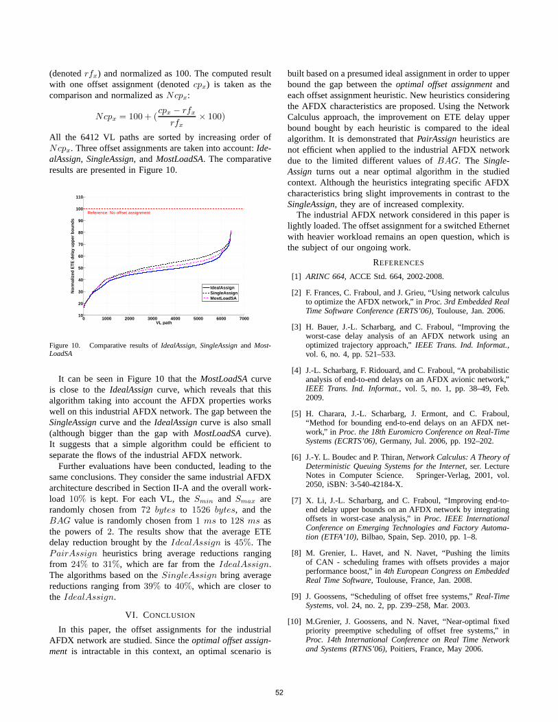
(denotedrfx) and normalized as 100. The computed resultwith one offset assignment (denotedcpx) is taken as thecomparison and normalized asNcpx:

Ncpx = 100 + (cpx − rfx

rfx× 100)

All the 6412 VL paths are sorted by increasing order ofNcpx. Three offset assignments are taken into account:Ide-alAssign, SingleAssign, andMostLoadSA. The comparativeresults are presented in Figure 10.

0 1000 2000 3000 4000 5000 6000 700010

20

30

40

50

60

70

80

90

100

110

Reference: No offset assignment

VL path

No

rmal

ized

ET

E d

elay

up

per

bo

un

ds

IdealAssignSingleAssignMostLoadSA

Figure 10. Comparative results ofIdealAssign, SingleAssignand Most-LoadSA

It can be seen in Figure 10 that theMostLoadSAcurveis close to theIdealAssigncurve, which reveals that thisalgorithm taking into account the AFDX properties workswell on this industrial AFDX network. The gap between theSingleAssigncurve and theIdealAssigncurve is also small(although bigger than the gap withMostLoadSAcurve).It suggests that a simple algorithm could be efficient toseparate the flows of the industrial AFDX network.

Further evaluations have been conducted, leading to thesame conclusions. They consider the same industrial AFDXarchitecture described in Section II-A and the overall work-load 10% is kept. For each VL, theSmin and Smax arerandomly chosen from72 bytes to 1526 bytes, and theBAG value is randomly chosen from1 ms to 128 ms asthe powers of2. The results show that the average ETEdelay reduction brought by theIdealAssign is 45%. ThePairAssign heuristics bring average reductions rangingfrom 24% to 31%, which are far from theIdealAssign.The algorithms based on theSingleAssign bring averagereductions ranging from39% to 40%, which are closer tothe IdealAssign.

VI. CONCLUSION

In this paper, the offset assignments for the industrialAFDX network are studied. Since theoptimal offset assign-ment is intractable in this context, an optimal scenario is

built based on a presumed ideal assignment in order to upperbound the gap between theoptimal offset assignmentandeach offset assignment heuristic. New heuristics consideringthe AFDX characteristics are proposed. Using the NetworkCalculus approach, the improvement on ETE delay upperbound bought by each heuristic is compared to the idealalgorithm. It is demonstrated thatPairAssignheuristics arenot efficient when applied to the industrial AFDX networkdue to the limited different values ofBAG. The Single-Assign turns out a near optimal algorithm in the studiedcontext. Although the heuristics integrating specific AFDXcharacteristics bring slight improvements in contrast to theSingleAssign, they are of increased complexity.

The industrial AFDX network considered in this paper islightly loaded. The offset assignment for a switched Ethernetwith heavier workload remains an open question, which isthe subject of our ongoing work.

REFERENCES

[1] ARINC 664, ACCE Std. 664, 2002-2008.

[2] F. Frances, C. Fraboul, and J. Grieu, “Using network calculusto optimize the AFDX network,” inProc. 3rd Embedded RealTime Software Conference (ERTS’06), Toulouse, Jan. 2006.

[3] H. Bauer, J.-L. Scharbarg, and C. Fraboul, “Improving theworst-case delay analysis of an AFDX network using anoptimized trajectory approach,”IEEE Trans. Ind. Informat.,vol. 6, no. 4, pp. 521–533.

[4] J.-L. Scharbarg, F. Ridouard, and C. Fraboul, “A probabilisticanalysis of end-to-end delays on an AFDX avionic network,”IEEE Trans. Ind. Informat., vol. 5, no. 1, pp. 38–49, Feb.2009.

[5] H. Charara, J.-L. Scharbarg, J. Ermont, and C. Fraboul,“Method for bounding end-to-end delays on an AFDX net-work,” in Proc. the 18th Euromicro Conference on Real-TimeSystems (ECRTS’06), Germany, Jul. 2006, pp. 192–202.

[6] J.-Y. L. Boudec and P. Thiran,Network Calculus: A Theory ofDeterministic Queuing Systems for the Internet, ser. LectureNotes in Computer Science. Springer-Verlag, 2001, vol.2050, iSBN: 3-540-42184-X.

[7] X. Li, J.-L. Scharbarg, and C. Fraboul, “Improving end-to-end delay upper bounds on an AFDX network by integratingoffsets in worst-case analysis,” inProc. IEEE InternationalConference on Emerging Technologies and Factory Automa-tion (ETFA’10), Bilbao, Spain, Sep. 2010, pp. 1–8.

[8] M. Grenier, L. Havet, and N. Navet, “Pushing the limitsof CAN - scheduling frames with offsets provides a majorperformance boost,” in4th European Congress on EmbeddedReal Time Software, Toulouse, France, Jan. 2008.

[9] J. Goossens, “Scheduling of offset free systems,”Real-TimeSystems, vol. 24, no. 2, pp. 239–258, Mar. 2003.

[10] M.Grenier, J. Goossens, and N. Navet, “Near-optimal fixedpriority preemptive scheduling of offset free systems,” inProc. 14th International Conference on Real Time Networkand Systems (RTNS’06), Poitiers, France, May 2006.

52

paper preprints rtn'2011 - teesside universitysst-web.tees.ac.uk/external/u0025697/rtn/rtn2011...

Documents