1

Paper SAS 552-2017

Deploying SAS® on Software-Defined and Virtual Storage Systems

Tony Brown, SAS Institute Inc., Addison, TX

ABSTRACT

This paper presents considerations for deploying SAS® Foundation across software-defined storage (SDS) infrastructures, and within virtualized storage environments. There are many new offerings on the market that offer easy, point-and-click creation of storage entities with simplified management. Internal storage area network (SAN) virtualization also removes much of the hands-on management for defining storage device pools. Automated tier software further attempts to optimize data placement across performance tiers without manual intervention. Virtual storage provisioning and automated tier placement have many time-saving and management benefits. In some cases, they have also caused serious unintended performance issues with heavy large-block workloads, such as those found in SAS Foundation. You must follow best practices to get the benefit of these new technologies while still maintaining performance. For SDS infrastructures, this paper offers specific considerations for the performance of applications in SAS Foundation, workload management and segregation, replication, high availability, and disaster recovery. Architecture and performance ramifications and advice are offered for virtualized and tiered storage systems. General virtual storage pros and cons are also discussed in detail.

INTRODUCTION

The advent of virtualization has enabled storage products that dramatically ease and accelerate storage creation and provisioning efforts, as well as storage expansion, migration, and high availability. The adoption of Software Defined Storage (SDS), and SDS elements, often simplify the storage management task to a point-and-click interface (a “single pane of glass” is the industry term). These new storage paradigms and features come in many types of architecture and offerings. These offerings pursue the goal to maximize storage resource utilization with minimal hands-on management and intervention often to the detriment of heavy workloads requiring thicker provisioning.

This paper will discuss how physical to logical abstraction supports storage virtualization. It will outline the major types of virtual offerings available including hypervisor-based systems like VMware® with traditional component systems, Converged Infrastructures (CI), and Software Defined Storage (SDS) managed Hyper-Converged Infrastructures (HCI). It will discuss the architectural and physical strengths and underlying physical weaknesses of each for SAS Foundation large block workloads. Also addressed will be specific problem areas in virtual storage architectures, including provisioning to physical resources, and practical steps to take to ensure adequate storage performance for SAS Foundation.

The discussion will begin with storage abstraction, the enabling technology to provide virtual storage.

STORAGE ABSTRACTION – FROM PHYSICAL TO VIRTUAL

HOW STORAGE IS MADE ABSTRACT - LUNS

Your first introduction to abstraction might have been your Algebra I class in high school. You were given puzzling problems to solve involving X and Y. X and Y were abstract equation variables that represented some number which you had to derive by solving an equation. If you liked puzzles, you loved this new discovery and could appreciate the power of abstraction as you moved on to higher algebraic learning. If you didn’t, you probably hated it and thought it totally useless. Abstraction is incredibly powerful when it comes to storage mapping and management.

Traditional storage methods use physical address mapping across Hard Disk Drives (HDD)/Solid State Drives (Flash – SSD) in a RAID Stripe. We typically work at the logical unit number (LUN) , which represents an address marker on a hardware device (typically a Redundant Array of Independent disks (RAID) device stripe across HDDs and SSDs). In non-virtualized storage, a SAS file system was typically

2

created from the operating system (OS) host, using a logical volume (LVM), which was defined as sitting on top of a LUN, or a stripe across multiple LUNs. This “logical volume” view of the physical was an abstraction, just a pointer to something physical. All the user can see is their file system name, they are not aware of the LUNs and physical device arrangement underneath them.

There are two primary forms of storage abstraction, hypervisor based virtual definitions, and proprietary virtual definitions as is common in vendor-based hyper-converged storage. We will discuss hypervisor based abstraction first.

A virtual LUN is created by hypervisor software, as a pointer to existing physical LUN(s) on a storage subsystem. A virtual LUN is created with a piece of hypervisor software (for example, VMware), by using a metadata table that takes the address of a large physical LUN or LUN(s) on storage, and mapping them to a virtual LUN definition for the virtual layer (for example, VMware® vSphere®) to exploit. In the case of VMware vSphere, this virtual LUN definition can be used to create a Virtual Machine File System (VMFS). The metadata translation of the physical storage LUN address to a virtual LUN address, is the abstraction point. Now any management operations on the virtual LUN are generally independent of the physical LUN characteristics underneath. The virtual LUN can be acted upon by VMware vSphere services and utilities to move the VMFS from one storage pool to another, snapshot it, clone it, and so on. without having to alter or deal with the underneath physical storage definition. Abstraction has taken us from managing the physical, to managing the virtual, over large pools of available physical storage. The large pools of physical storage ostensibly only have to be set up once. They aren’t like managing small pools that have to be backed up individually, expanded in size frequently, and so on. We can now handle most of the storage management aspects with a point-and-click virtual interface that rides on top of the physical layer, in a virtual hypervisor. This is the power of abstraction, and what it enables – virtualization.

HOW STORAGE IS MADE ABSTRACT – WITHOUT LUNS

Some hyper-converged storage infrastructures present other non-LUN methods to map physical storage to a virtual storage pool. One example is to use a proprietary software RAID mechanism that combines most or all the storage array devices into a single large pool in a just-a-bunch-of-disks arrangement (JBOD). This proprietary software RAID does not require physical LUN address mapping and is part of a software defined storage system. The defined “large pool” consists of all the available HDD and SSD devices in the pool definition and is then presented to the virtual layer as a virtual abstraction of the pool to the virtual hypervisor, or software-defined storage layer. An example of this type of presentation is IBM Elastic Scale Storage (ESS).

Storage abstraction is an underlying enabler of virtual hypervisor controlled systems, and other proprietary mapping systems in the previous example. The next section will discuss virtual storage on the following:

Traditional discrete component storage systems (physical server nodes, virtual machines (hypervisor layer), fabric (direct-attached Fiber Channel, network attached), and storage arrays.

Converged System Infrastructures (CI)

VIRTUAL STORAGE MECHANISMS FOR TRADITIONAL COMPONENT AND CONVERGED INFRASTRUCTURES

This section of the paper will address how storage virtualization is implemented using legacy component systems and Converged Infrastructures (CI). It will begin with the use of hypervisor virtualization layers such as VMware on component systems, which is ubiquitous in today’s environment. It will then discuss physical storage virtualization within large arrays that support abstraction to the hypervisor controlled virtual layers.

Prior to the advent of Converged (CI) and Hyper-Converged Infrastructures (HCI), the world was composed of what we will call traditional component systems — hosts, storage, networks — with virtual

3

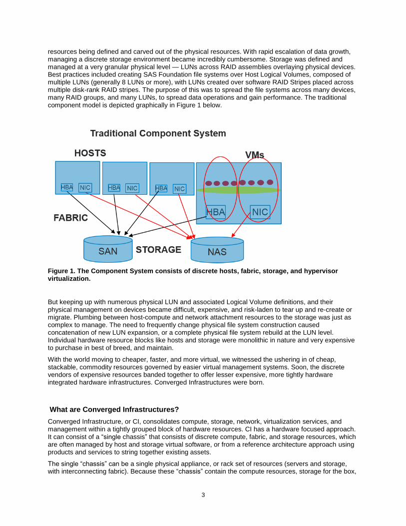
resources being defined and carved out of the physical resources. With rapid escalation of data growth, managing a discrete storage environment became incredibly cumbersome. Storage was defined and managed at a very granular physical level — LUNs across RAID assemblies overlaying physical devices. Best practices included creating SAS Foundation file systems over Host Logical Volumes, composed of multiple LUNs (generally 8 LUNs or more), with LUNs created over software RAID Stripes placed across multiple disk-rank RAID stripes. The purpose of this was to spread the file systems across many devices, many RAID groups, and many LUNs, to spread data operations and gain performance. The traditional component model is depicted graphically in Figure 1 below.

Figure 1. The Component System consists of discrete hosts, fabric, storage, and hypervisor virtualization.

But keeping up with numerous physical LUN and associated Logical Volume definitions, and their physical management on devices became difficult, expensive, and risk-laden to tear up and re-create or migrate. Plumbing between host-compute and network attachment resources to the storage was just as complex to manage. The need to frequently change physical file system construction caused concatenation of new LUN expansion, or a complete physical file system rebuild at the LUN level. Individual hardware resource blocks like hosts and storage were monolithic in nature and very expensive to purchase in best of breed, and maintain.

With the world moving to cheaper, faster, and more virtual, we witnessed the ushering in of cheap, stackable, commodity resources governed by easier virtual management systems. Soon, the discrete vendors of expensive resources banded together to offer lesser expensive, more tightly hardware integrated hardware infrastructures. Converged Infrastructures were born.

What are Converged Infrastructures?

Converged Infrastructure, or CI, consolidates compute, storage, network, virtualization services, and management within a tightly grouped block of hardware resources. CI has a hardware focused approach. It can consist of a “single chassis” that consists of discrete compute, fabric, and storage resources, which are often managed by host and storage virtual software, or from a reference architecture approach using products and services to string together existing assets.

The single “chassis” can be a single physical appliance, or rack set of resources (servers and storage, with interconnecting fabric). Because these “chassis” contain the compute resources, storage for the box,

4

network, and virtualization services, they can usually be ‘stacked’ or scaled as units for scale-out growth. With data centers trying to overcome compatibility issues between disparate hardware offerings, and reduce ownership costs, the CI infrastructure is very attractive. It allows scale-out without reconfiguring existing monolithic resources. Figure 2 below shows a basic diagram of a chassis instance of CI.

There are some offerings, EMC VSPEX for example, that provide converged infrastructure services, while allowing use of independent hardware. This can be used to leverage known compatible hardware already used at a site. In this case the VSPEX provides a reference architecture provider to guide inclusion of non-integrated compute, fabric, and storage resources. These resources would consist of a virtualization provider like VMware, end user, compute, fabric, switch, and storage resources from multiple vendors.

If the CI “single chassis” is a pre-configured appliance or rack resource set, it isn’t typically as flexible to alter their configurations after they are installed. And when expanding, you can’t just add storage, or compute, or memory, easily. You are essentially adding a preconfigured appliance to increase resources, with set ratios of pre-packaged compute, fabric, and storage provisioning. If the CI “box” is a block set of resources (for example, separate servers, fabric, and storage blocks with tight physical co-location - for example, rack set), the resources can be used outside the single CI instance, and can be scaled separately in an easier fashion.

Many CI Vendors use VMware vSphere to create both host and storage virtualization for their converged systems. An example of a CI vendor using VMware is the VCE VBLOCK system. This is a converged system built in partnership between CISCO, EMC, and VMware to provide a virtual computing environment of converged compute, fabric, storage, and virtualization services in a block unit. This block of resources can be easily acquired, implemented, and managed as a “start small and grow” scale-out approach.

Figure 2. The Converged Infrastructure chassis offering consists of tightly co-located compute, fabric, virtualization, and storage resources as a “stackable” block unit, designed for scale-out growth.

For converged systems, the utilization of a virtual hypervisor (for example, VMware) provides the virtualization services for both the compute resources as well as storage. This type of offering is primarily a hardware driven assembly, for unified support, scale-out, and snap-in resource acquisition. The bottom line with CI is that it is tightly integrated hardware.

5

Storage virtualization is one of the drivers for CI systems to succeed. We will first address hypervisor virtualization capabilities for component storage, and CI, using VMware and its related product set as our example.

VMWARE HYPERVISOR STORAGE VIRTUALIZATION

Why address VMware first? VMware has long been known for its successful host virtualization offerings in traditional component systems, as in Figure 1 above. VMware also offers storage virtualization and management products. Given its dominance of the marketplace and ubiquitous nature, it is often chosen for platform virtualization services by converged storage vendors (more on this later). VMware vSphere supports multiple forms of virtualization on traditional storage. This discussion will focus on the Virtual Machine File System (VMFS), using Virtual Machine Disks (VMDKs) and Raw Device mapping (RDM).

VMware VMFS is a virtual cluster file system. It allows sharing of multiple VM hosts to the VMFS file space, maintaining lock coherency across the VM hosts and their respective VMDKs. A VMFS is typically mapped to a physical LUN or set of LUNs on a storage system. The placement of the physical LUN(s) across storage devices is crucial. Placing a LUN across too few devices can result in poor aggregation of device bandwidth and adversely affect performance. It is typical to try to spread the LUN stripes across all of the devices in a large, thin storage pool.

The size limit of a VMFS LUN for VMFS 5.5.x and later is 64 Terabytes (TB). There is an extent limit of 32 LUNs per VMFS instance. This means that a VMFS that is 64 TB in size, can be composed of one 64 TB LUN, thirty-two 2 TB LUNs, or any combination in-between. If only one or a few extents exist, and more capacity is needed, the VMFS can be expanded by adding additional physical LUN(s)/extents to the VMFS definition, up to a 64 TB total. This is a capacity-add, the physical LUNs comprising a VMFS are not striped together at the physical layer. Instead, they are striped across devices and this stripe is where device aggregation occurs. The capacity add allows additional VMDKs (see below) to be added to the VMFS, on the space of the added LUN. As stated, there isn’t a concept of striping the VMFS across multiple LUNs, such as in a host-striped Logical Volume. The behavior of the underlying VMFS LUNs is more concatenated in nature.

With VMFS 5.5.x and later, mapping is accomplished via ATS VAAI primitives. There is a limit of 256 LUNs in an ESXi® server, and for each VM host. Planning is required for LUN sizing and creation. Because single LUN performance can often be what was engineered, placement of the LUN definition across many or all available physical devices in a large, thin pool is important. If you have few physical devices beneath your storage LUN, inadequate bandwidth can result.

Once created, a VMFS can then be populated with two major types of storage entities: Virtual Machine Disks (VMDKs), and Raw Device Mapping instances.

In addition, each VMFS has a limited queue depth (simultaneous active requests) of 32. It is easy to overrun this queue, and multiple VMFS entities might be required to garnish additional queue depth. This is typically one of the first bottlenecks in very busy VM systems.

One of the crucial challenges with VMFS is backing it with performant physical LUNs.

Another of the crucial challenges with VMFS is creating enough VMFS instances to attain adequate working queue depth.

6

VMware Virtual Machine Disks (VMDK)

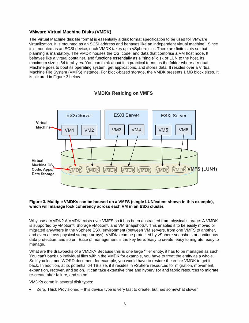
The Virtual Machine disk file format is essentially a disk format specification to be used for VMware virtualization. It is mounted as an SCSI address and behaves like an independent virtual machine. Since it is mounted as an SCSI device, each VMDK takes up a vSphere slot. There are finite slots so that planning is mandatory. The VMDK houses the OS, code, and data that comprise a VM host node. It behaves like a virtual container, and functions essentially as a “single” disk or LUN to the host. Its maximum size is 64 terabytes. You can think about it in practical terms as the folder where a Virtual Machine goes to boot its operating system, get applications, and stores data. It resides over a Virtual Machine File System (VMFS) instance. For block-based storage, the VMDK presents 1 MB block sizes. It is pictured in Figure 3 below.

Figure 3. Multiple VMDKs can be housed on a VMFS (single LUN/extent shown in this example), which will manage lock coherency across each VM in an ESXi cluster.

Why use a VMDK? A VMDK exists over VMFS so it has been abstracted from physical storage. A VMDK is supported by vMotion®, Storage vMotion®, and VM Snapshots®. This enables it to be easily moved or migrated anywhere in the vSphere ESXi environment (between VM servers, from one VMFS to another, and even across physical storage arrays). VMDKs can be protected by vSphere snapshots or continuous data protection, and so on. Ease of management is the key here. Easy to create, easy to migrate, easy to manage.

What are the drawbacks of a VMDK? Because this is one large “file” entity, it has to be managed as such. You can’t back up individual files within the VMDK for example, you have to treat the entity as a whole. So if you lost one WORD document for example, you would have to restore the entire VMDK to get it back. In addition, at its potential 64 TB size, if it resides in vSphere resources for migration, movement, expansion, recover, and so on. It can take extensive time and hypervisor and fabric resources to migrate, re-create after failure, and so on.

VMDKs come in several disk types:

Zero, Thick Provisioned – this device type is very fast to create, but has somewhat slower

7

performance on “first writes” to the device. This is the standard way to create a new VMDK by administrators.

Eager Zero, Thick Provisioned – this device type takes a bit longer to create, but has better performance on “first writes” to the device. This is typically done when cloning an existing VMDK.

Thin Provisioned - this device type is very fast to create the VMDK, but has much poorer write performance on all writes to the device. In addition, underlying physical storage must be constructed as thin provisioned as well or the operations don’t mesh, and won’t go well.

In addition to the disk type, there are several available disk modes to choose from when creating the VMDK:

Independent, Persistent – this mode forces all VM WRITES to device for persistent availability to support recovery. This mode generally has the best performance overall, especially when recovering a VMDK.

Independent, Non-Persistent - this mode only keeps non-persistent changes in device WRITES. It has relatively poor performance in general, and especially in recovery.

Snapshot – this mode does not track persistent changes and can only return to its previous state in recovery.

IO Flow is crucial to good performance in a VMware ESXi system. Process bandwidth, and plumbing throughout the virtual and physical path must be replete. There are several places in the virtual and physical architectures that become choke points to either processes or IO. They include, but are not limited to the following:

IO Performance Choke Point Areas:

o Host Adapter Bandwidth

o Host Adapter Queue Depth Settings – Adapters have finite LUN queue depth settings, with low defaults.

o Storage Array Port Queue Depths

o Storage Array Controller Bandwidth

o Storage Device Count and Physical LUN Spread across Pools

o Number of VMFS LUNs Provisioned to SCSI Initiators, VMFS Queue Depths

o Number of VMDKs Provisioned per VM LUN

One of the primary issues with VMFS entities is the aggregation of bandwidth across many storage devices, disk (HDD), and flash (SSD). In bare metal systems running SAS Foundation software, the best

When choosing the VMDK disk type for SAS Foundation we typically recommend the Eager Zero, Thick Provisioned type.

When choosing the VMDK disk mode for SAS Foundation we recommend the Independent, Persistent mode.

8

practice is to create at least 8 LUNs per SAS file systems in a Logical Volume. SAS can write in parallel to each LUN, aggregating the bandwidth throughput of the devices under that LUN. 8 LUNs give you approximately 8x the throughput in MB/sec as 1 LUN would. Not being able to stripe across LUNs can be a VMFS throughput restriction as compared to Logical Volumes with striped LUNs on bare metal. See Figure 4 below for an illustration. If you lack adequate IO bandwidth from your existing VMFS LUNs definitions, you might have to resort to creating LUNs across all the devices in an array. This might help, but still might not equal the performance of striped LUNs in a Logical Volume.

Figure 4. VMFS essentially concatenates LUN extents. While LUNs are striped across the device pool, the LUNs are not striped together like an LVM definition. It is easier to add capacity this way, but this loses parallel LUN WRITES that SAS benefits from. You must ensure that LUNs are striped across very large, thin pools to aggregate device performance adequately.

VMware Raw Device Maps (RDM)

Raw Device Maps (RDM) is a mapping file that can be created in a VMFS volume that acts as a pointer to, or a proxy for a raw physical device. RDMs are connected via an SCSI device, which is used directly by a virtual machine. The RDM contains metadata for managing and redirecting disk access to a defined physical device. In short, it is a pointer to physical back-end storage for the VM node. It appears as a normal disk file to the VM node, and has typical file systems operations and services. Because the RDM is mounted via an SCSI device, each RDM requires an SCSI device port in the VM node. An illustration of how an RDM is addressed is in Figure 5 below.

9

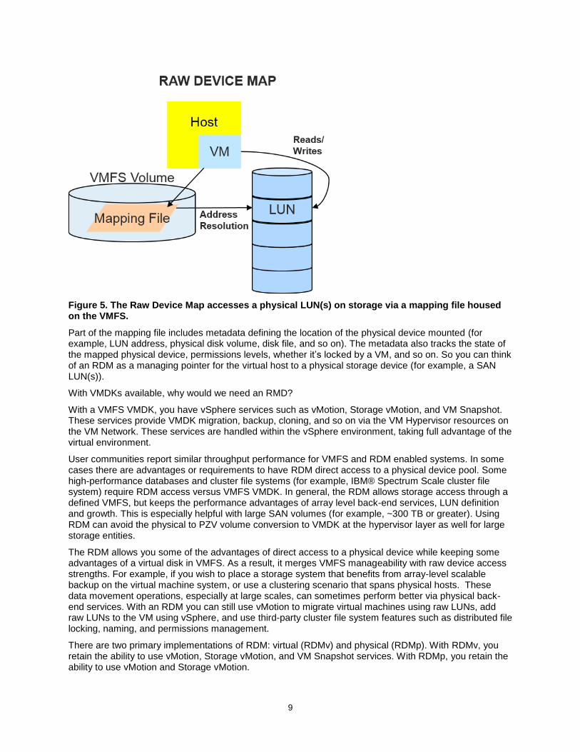
Figure 5. The Raw Device Map accesses a physical LUN(s) on storage via a mapping file housed on the VMFS.

Part of the mapping file includes metadata defining the location of the physical device mounted (for example, LUN address, physical disk volume, disk file, and so on). The metadata also tracks the state of the mapped physical device, permissions levels, whether it’s locked by a VM, and so on. So you can think of an RDM as a managing pointer for the virtual host to a physical storage device (for example, a SAN LUN(s)).

With VMDKs available, why would we need an RMD?

With a VMFS VMDK, you have vSphere services such as vMotion, Storage vMotion, and VM Snapshot. These services provide VMDK migration, backup, cloning, and so on via the VM Hypervisor resources on the VM Network. These services are handled within the vSphere environment, taking full advantage of the virtual environment.

User communities report similar throughput performance for VMFS and RDM enabled systems. In some cases there are advantages or requirements to have RDM direct access to a physical device pool. Some high-performance databases and cluster file systems (for example, IBM® Spectrum Scale cluster file system) require RDM access versus VMFS VMDK. In general, the RDM allows storage access through a defined VMFS, but keeps the performance advantages of array level back-end services, LUN definition and growth. This is especially helpful with large SAN volumes (for example, ~300 TB or greater). Using RDM can avoid the physical to PZV volume conversion to VMDK at the hypervisor layer as well for large storage entities.

The RDM allows you some of the advantages of direct access to a physical device while keeping some advantages of a virtual disk in VMFS. As a result, it merges VMFS manageability with raw device access strengths. For example, if you wish to place a storage system that benefits from array-level scalable backup on the virtual machine system, or use a clustering scenario that spans physical hosts. These data movement operations, especially at large scales, can sometimes perform better via physical back-end services. With an RDM you can still use vMotion to migrate virtual machines using raw LUNs, add raw LUNs to the VM using vSphere, and use third-party cluster file system features such as distributed file locking, naming, and permissions management.

There are two primary implementations of RDM: virtual (RDMv) and physical (RDMp). With RDMv, you retain the ability to use vMotion, Storage vMotion, and VM Snapshot services. With RDMp, you retain the ability to use vMotion and Storage vMotion.

10

The same precepts of physical LUN count apply to RDMs as to VMDKs above. Work closely with your file systems or database vendor if they require RDMs for their products.

CHOKE POINTS FOR VMFS PROVISIONED STORAGE

IO flow is crucial to good performance in a VMware ESXi system. Process bandwidth and plumbing throughout the virtual and physical path must be replete. There are several places in the virtual and physical architectures that become choke points to either processes or IO. They include, but are not limited to the following:

Virtual Choke Point Areas:

o Number of VMFS LUNs Provisioned to SCSI Initiators – the number of SCSI initiators must be carefully considered when provisioning VMFS instances. Each VMFS instance is an SCSI connection to the host. SCSI ports are finite, so provision the underlying resources adequately.

o ESXi SCSI Initiator Queue Depth Settings – SCSI device drivers (Host Bus Adapters (HBAs)) have a configurable LUN queue depth setting to determine how many active commands can be present on a single LUN. QLogic Fiber Channel HBA’s support up to 255 simultaneous commands, and Emulex up to 128. The default value for both is 32. If an ESXi host generates more requests to a LUN than this queue depth, the excess requests are backed up on the ESXi host, building latency. This queue depth setting is per LUN, not per initiator (HBA).

o There is also a VMware VirtualCenter configuration parameter, Disk.SchedNUMReqOutstanding, which governs the queue depth setting for Multiple VMs to a single LUN. When this setting is exceeded, latency backs up on the EXSi kernel. If this setting is used in the case of multiple VMs attached to the same LUN, it must be set at the same queue depth as the SCSI initiators.

o It is also important to note that if multiple ESXi hosts attach to the same storage array LUN, and each generates is maximum number of queue requests, it is possible to overload the array’s ability to manage all the incoming LUN requests, and latency can build up on the array device level.

o Best practices to avoid queuing at the storage device level include:

Setting a maximum LUN queue depth of 64 for each ESXi VM host (if multiple hosts attach to a single LUN)

Setting a maximum LUN queue depth of 128 for individual ESXi hosts that exclusively attach to a single LUN

Ensure that the storage array model does not have a per-LUN queue restriction

Ensure there are enough physical devices in the array to support the demand load without overloading the device layer

Provide enough LUNs to aggregate queue depth for high performing file systems such as IBM Spectrum Scale (for example, provision at least 8 LUNs for this type of file system)

o Sheer LUN Count is Key. Each ESXi host can support up to 256 LUNs. This must be tempered to stay within the SCSI initiator availability, VMFS queue depth settings, HBA queue depths, and Fiber Channel throughput to the storage. But multiple LUNs are required to gain additional raw device aggregation underneath per LUN, and provide additional LUN queues to drive workload.

o Provide enough VMFS instances to provide more queue depth. Ensure that each VMFS LUN is striped across enough back-end devices to carry the load presented from the SCSI initiators. It won’t help to bump up the queue depths if there aren’t enough back-end devices

11

to service the outstanding request levels.

Additional Physical Choke Point Areas:

o Ensure that the storage array Port queue depths are not depleted (work with your Storage Administrators)

o Ensure that the Array Controller Bandwidth is not violated (many arrays have a dual controller design; some are integrated). Again, work with your Storage Administrator.

o SAN Fiber Channel switch ports have a setting called buffer credit. The unit of transfer in Fiber Channel technology is called the frame. Frames house everything transported over the FC path. Frame management is the flow control mechanism across Fiber Channel medium. The buffer credit is the allowable number of frames a port can actively store at once, before it fills up, and frames have to be emptied (used and acknowledged to make room for more). So buffer credits are used to regulate flow. Normally the default frame count is more than enough but every once in a while you will run into a performance case where that number needs to be increased. This can be the case on heavily loaded ESXi servers cabled over long distance to storage, or residing on fabric interconnect that doesn’t contain adequate bandwidth or is too congested. In this case raising the buffer credits value can alleviate halts in frame transfers. But it will do this at the expense of putting more pressure on the back-end LUNs and underlying storage.

o Ensure that the physical LUN created to back a VMFS LUN is spread across as many devices as possible, preferably on all the devices in a large thin pool. A VMFS can span LUNs for additional capacity, but it doesn’t stripe across LUNs. This limits performance to the aggregated device count in a RAID stripe under each LUN. It is crucial to get as much device (HDD, SSD) aggregation as possible for throughput performance.

We have discussed VMware storage virtualization in detail. We will now touch on some array-level technologies that enable greater virtualization management at the hypervisor and software defined storage (SDS) layers.

ARRAY LEVEL ENABLERS OF STORAGE VIRTUALIZATION

INSIDE THE SAN VIRTUALIZATION

For some time there have been virtualizing enablers or technologies at the storage array level. These include technologies that provide:

De-duplication and compress storage for reduced capacity, metadata driven management, and ease of migration services.

Policy-driven automated tier management software that allows data to be promoted or demoted across various levels of performant storage (HDD, SSD device pools).

Virtual controllers for SAN volume management and data placement to consolidate the above technologies into a virtually managed system (for example, IBM SAN Volume Controller).

On many modern storage arrays, advanced services are offered to better physically manage workload, and performance. These features include data compression, encryption, and block de-duplication. Compression and encryption are long-standing features in many arrays. Data de-duplication in recent years has involved metadata and hash table management of mapping data blocks that are duplicate (often a 4K block size) to the address of the identical physical block already stored on device. These metadata “pointers” now provide this unique block address to any file definition needing that block. We have seen reductions of up to 5 or 6 x on some data populations using this method. Combined with compression, space savings can be very significant. By drastically reducing the amount of data being backed up, migrated across performance tiers (discussed below), and so on., these features significantly

12

reduce data volume for back-end array services like snap/clone, migration, backup, HA, and so on. This reduced workload volume also makes it more attractive to move these types of services to the hypervisor/software layer of virtual management. The reduced workload might now fit within the network fabric infrastructure of the virtual machine environment, making it possible for some workloads to be moved from the back-end array where they traditionally reside due to volume and performance.

Many arrays consist of performance tiers of storage, with various capacities and rotational speeds of spinning disk (HDD), and flash storage units (SSD). The various layers of HDD and SSD storage offer capacity versus performance trade-offs. Automated Tier Management Software in modern arrays provides policy driven (you write the policies) management of data movement and migration across performance tiers. You can set dynamic policies to place highly used data in performant flash storage (SSD), lesser used data on slower hard disk drives (HDD). You can set migration to be “on-the-fly” to begin migrating data while a large job set is running against it, or re-tier on a 24-hour basis for example, based on the previous day’s usage.

Many storage arrays offer the above services “in array”. Meaning they are part of the storage array features package. For traditional component system shops, the above SAN level features have provided significant storage performance improvement. They have also been used as enabling features to empower other virtualization layer products. IBMs SAN Volume Controller (SVC) is an example of that. It removes array-side management of those features to a software controlled server that can operate across multiple SAN entities, while providing high availability services.

These array level services that either virtualize or support virtualization of resources can have deleterious effects. Here are some best practices in using them:

Pin SAS file systems to particular storage tiers (SSD, SAS, and so on.) and avoid migration when possible. If migration must take place on large files, or file systems it should be considered on a 24-hour boundary, to be accomplished by back-end array services when the system can afford the resources to do so. Any live migrations during busy periods tend to be too slow for SAS Foundation’s large, fast consumption of large-block data files. By the time the migration is in play, the SAS operation is typically already in a latent state.

Do not place SAS files on lower performing tiers such as SATA, near-line storage, and so on. Unless the files are planning on being in “archive” mode, these tiers do not perform well enough to guarantee our minimum needed bandwidth of 100 – 150 MB/sec per Core for the host systems.

Array Service Compression utilities typically perform adequately without adding undue latency to READ/WRITE services. However, inline data de-duplication typically does not. You will have to test the de-duplication services on the array models you use to determine if they are beneficial or harmful in terms of performance.

Be mindful of virtual management interfaces that benefit from these array side features, or actually take control of them at the software layer. What is happening at the physical device layer cannot be forgotten.

The above array-level enablers reduce data volumes on device very significantly. By reducing data, making it easier to migrate, it can now become a better candidate to handle at the hypervisor/software management layer of a virtual system. Some of these data volumes might now fit within the bandwidth limitations of the virtual fabric infrastructure. These technologies have evolved to become enablers of Software Defined Storage (SDS) and Hyper-Converged systems.

SOFTWARE DEFINED STORAGE – ENABLING HYPERCONVERGED STORAGE SYSTEMS

Hyper-Converged infrastructures (HCI) are similar to CI, but introduce an additional layer of tighter, software-driven integration between the compute, storage, network, and virtualization components. See

13

Figure 6 below. It starts with the CI resources, but can move array-level services like backups, snapshots, data de-duplication, inline compression, LAN/WAN optimization, and policy driven storage management to the virtualized software management layer. CI is primarily hardware focused. HCI with software defined storage (SDS) virtual management is typically hardware agnostic, providing a software interface to create, control, and manage storage. HCI can remove some of the storage management functions from the physical storage layer, placing them in the SDS control environment. These include functions like compression, encryption, de-duplication, policy driven storage movement across tiers and platforms, and so on. A key benefit of HCI offerings is they are typically supported by a single vendor (who owns the entire stack of host, fabric, storage, and virtualization), with tight management integration to support scalability. There are numerous HCI vendors, and each HCI system might use a tightly integrated proprietary product set of host, fabric, storage, and virtualization. This integrated product set is typically supported by a single entity representing the product set. It also supports more infrastructure flexibility in configuring resources for varying workloads, thanks to the SDS facilities. For scaling, you can snap on another box, or re-configure existing boxes with SDS resources more easily.

Figure 6. The Hyper-Converged Infrastructure (HCI) with software defined storage becomes more hardware agnostic, focusing on software integration and management of storage. This example shows a chassis infrastructure, but SDS Offerings for discrete resources are available.

14

WHAT IS SOFTWARE DEFINED STORAGE?

Single Pane of Glass Management

Software Defined Storage (SDS) is essentially a software mechanism that can provide provisioning and management of data storage that is independent of the underlying hardware and hardware management. It is often referred to as a “single pane of glass”, meaning a point-and-click GUI interface with which an administrator can literally create, move, grow, replicate, back up, and so on., storage entities (pools, file systems, virtual LUNs, and so on). SDS typically uses, but does not always require, several underlying technologies such as abstraction, storage virtualization, pooling, and automation software for storage policy management. Traditional SAN-level services such as data de-duplication or thin provisioning management, and replication are contained in some SDS architectures. These supporting technologies can be provided by the SDS package itself, or might reside within third-party software tools, or SAN service facilities that the SDS package can interface with.

SDS is a generic term for a broad array of product offerings from many vendors with different features and functionality mixes. The differences, and hence the pros and cons of all these offerings, can be quite confusing, hence difficult to evaluate. SDS can be used to manage traditional block storage in a storage array network (SAN), or with network attached, or file-based storage (NAS). Some newer SDS offerings interface with object-based storage systems.

Why SDS?

Managing physical storage is incredibly difficult. The old methods of creating, tuning, changing, and implementing high availability for physical file systems was cumbersome, expensive, and very time consuming. There were incremental limitations on how to expand underlying RAID rank resources for striped LUNs for example. Each file system had to be managed independently from a physical level. With rapidly expanding storage footprints, the costs became prohibitive. Market vendors responded with new product offerings using methods and technologies to allow an abstraction of physical storage to virtual definitions. These virtual definitions are the cornerstone of the ease of management features that empower SDS.

With this new “single pane of glass approach”, an administrator can use a single administrative UI to create a virtual file system from scratch, grow it, move it around, change its underlying makeup of storage type, replicate it back it up, make it highly available, shrink it, or destroy it. All this can be done with the touch of a button. Compared to the physical manipulation of traditional SAN or NAS file systems, this is like heaven for administrators. It has brought to storage what host virtualization has given the server side of the community for some time now.

So what are the primary goals of using SDS? Obviously a tremendous time savings and ease of management for administrators. Because some SDS offerings are designed around commodity hardware usage, there are obvious hardware cost savings but these can be offset by the expense of the HCI software license costs. Like the goals of most virtualized systems, easier management of storage resources can aid in driving utilization of existing shared resources higher. By creating virtual file systems or file storage on shared resources, it is very easy to thin provision the storage space, allowing more virtual hosts access to it, and drive up resource utilization. All these things are very attractive in terms of total cost of ownership, deployment speed, and easier and less expensive management costs.

Some SDS offerings are packages of compute, network, and storage resources, similar to the CI chassis presented above. And like the CI hardware arrangement, this can be used to more easily scale out growth. Scale-out expansion is more cost effective, easier to manage, and typically much easier to implement. It can offer lower initial cost of ownership (depending on license costs), incremental growth, and hardware savings when commodity hardware is used. Many SDS vendors have interfaces for VMware products, and services for their Hyper-converged system offerings such as VxRail Others have proprietary virtualization and software defined management products.

15

GENERAL PROS AND CONS OF HCI WITH SOFTWARE DEFINED STORAGE

HCI typically offers very tightly integrated building block structures to work with, snap together, and scale from. The systems are supported by a single vendor, significantly simplifying support, troubleshooting, and deployment issues. The ease of resource deployment and resource administration is the primary cost level benefit, as commodity hardware savings can often offset by SDS licensing costs.

Because the technology is software defined and integrated, it cannot be easily broken in discrete block components like CI infrastructures. It is defined as a unit and pretty much stays that way. This means that alteration of the configuration after the fact isn’t typically possible. It also means that scalability is confined to pre-provisioned units of offering in terms of compute, storage, and fabric ratios. This could be expensive if only one resource area, for example, IO needs to be expanded.

Some newer technology offerings such as IBM Elastic Storage Server® (IBM ESS), using Spectrum Scale® software remove LUN address mapping to their HCI storage blocks. They use proprietary software RAID systems on wide, disparate device pools, negating the need for storage creation of or virtual mapping to physical LUNs. This can provide a better decoupling from physical storage in the sense that the granular level of LUN management is erased from the physical side. It is also a departure of how physical storage is provisioned beneath a virtual provider, as very large pool versus a narrow LUN stripe definition. By using the entire pool of storage as a single entity, device bandwidth can be greatly aggregated across many more devices. This translates into higher physical throughput in MB/sec.

When scaling out large numbers of HCI units, optimal data placement for utilization across the cluster becomes very important. You will need to investigate how data is co-located with compute resources on the cluster to avoid shipping of significant data volumes across the cluster interconnects. IBM ESS for example, offers a software tool to manage this, File Placement Optimizer (FPO). Intelligent data mapping that allows placement of physical data closest to the node using it the most, is crucial.

HCI infrastructures can experience many of the same underlying virtual and physical provisioning issues as CI and component systems. If HCI uses a hypervisor layer the same issues mentioned about VM provisioning and tuning apply. Areas of attention for non-hypervisor, proprietary storage virtual management in SDS are mentioned below:

Proprietary disk management structures HCI offerings that provide their own array level pool management structures (for example, proprietary RAID structures, and so on) can provide a variation on device pooling from physical LUN arrangements in large storage systems. You must work carefully with your HCI provider to ensure that the storage pool is physically sufficient to provide bandwidth for all the virtual structures defined on top of it in the SDS layer. The SDS interface is highly convenient and powerful. It will allow an administrator to resize, re-tier, migrate, and clone defined storage entities with the touch of a button. With large files and file systems this can be like a skinny tail wagging a big dog. Performance can be easier to manage, giving the SDS layer more latitude in such activity, but overall pool sharing and performance must be measured correctly and provisioned.

Data migration, placement, management from a hypervisor layer versus the array services layer With SDS and HCI, services for many of what were, array-level activities have been moved up to the hypervisor/software layer. This is a huge time save for administrators. The storage administrator need only provide large performant pools, the Hypervisor/SDS administrator can take over the daily management from there. There is no magic, or free lunch here. Just convenience. One must be careful to plan how much of these previous array-level services, with their potentially very high bandwidth, can subsist on the virtual software layer, and its underlying ports, initiators, and network fabric infrastructure! How much bandwidth can your network fabric bear if suddenly snap-

16

clones, backups, migrations, and so on begin occurring over it? Careful provision planning is needed.

Thin provisioning, utilization, and subscription via software defined structures One of the primary precepts of HCI and SDS is to drive higher utilization out of fewer resources, saving money, and reducing complexity and cost. If thin provisioned systems are over-subscribed, pain typically results. This is frequently the case with virtual storage entities defined to maximize underlying storage resources. SDS tools allow this to happen very easily because the knowledge of performance that is held by the Storage administrator is now abstracted to the SDS administrator. As with VMware above, this has been an issue for quite some time. The SDS administrator needs to clearly understand his physical resource limitations, and not get too zealous with thin provisioning. It can result in serious problems with SAS Foundation workloads.

Virtual storage management is the design of the future due to easy deployment, ephemeral nature, and reduced cost of ongoing management. Storage infrastructures are becoming highly integrated with compute and network tiers, with snap-together structures that can be scaled out at will. With its proliferation, how can you maintain the storage performance you need? We will review the physical considerations next.

PHYSICAL CONSIDERATIONS FOR VIRTUAL DEPLOYMENTS

THE PHYSICAL IO PATH – CHOKE POINTS

The physical performance path described in the various sections above is important to pay attention to in any system: bare-metal or virtualized. A top-to-bottom list is reiterated below for checkpoints.

Host Layer

1. Host OS/hypervisor tuning for memory and IO management

2. Host memory and file cache size, and tuning

3. Host and Hypervisor initiators to storage (HBA/NIC), bandwidth, speed, queue depth tuning

4. Host Multipath Arrangements for host defined paths to storage

Storage Layer

1. Storage FA ports and zoning, bandwidth, queueing, balance

2. Device pool arrangement for virtual servicing, LUN definitions, RAID levels, wide pool definitions. Ensure enough device aggregation to drive workload.

3. Storage device pool ability to service queue loads from multiple virtual file systems and hosts

If the above physical foundation is planned, virtual operations above it will perform well. The most trouble arises at the virtual layer when the underlying physical layer cannot meet workload performance requirements.

17

CONCLUSION

Storage virtualization is a complex subject with many layers and a variety of offerings and approaches. New product offerings are introduced almost monthly. Vendors appear regularly with new products and promises. Cloud technologies use the same virtual mechanisms as above and more. Cloud services providers are expanding virtual definitions and ephemeral definitions to extreme limits. The scope of this paper cannot contain the complexity of what is newly appearing and what is on the horizon. It can be extremely confusing to understand what currently exists and yet keep up with the flood of new techniques and products. But there are several precepts that can help tame the confusion. They can be used to evaluate virtual technology from several levels.

1. Understand IO requirements for SAS Foundation: http://support.sas.com/resources/papers/proceedings16/SAS6761-2016.pdf

http://support.sas.com/resources/papers/proceedings15/SAS1500-2015.pdf

2. Take the deep dive on the technology you are considering. Meet with the product storage engineers and understand their requirements for physical storage presentation to their virtual layer.

3. Everything virtual has to touch something physical at some point. You must trace the physical path of a virtual system. Is the physical resource provisioning underneath going to give you the throughput, bandwidth, and power you need to drive your workload?

4. Bare-metal storage infrastructures were a pain to manage, but they were somewhat like a custom car. Hard to build and change, but designed for your IO processing bandwidth needs. When custom storage designs are ameliorated to virtual definitions sharing large pools of storage, how much have my custom bandwidth needs been watered down? Compare what the virtual system is giving you in performance to a bare-metal system. It likely will not be the same, but is the reduction viable for the virtual ease-of-management benefits?

5. Review any available SAS Performance Lab Test Reviews. Most are for flash storage arrays, but increasingly for CI and HCI systems:

http://support.sas.com/kb/53/874.html

6. Work with your SAS Account Team, SAS Technical Resources, and virtualization product vendors for expert advice.

7. Measure, measure, measure. Map the virtual infrastructure from the top to the bottom, ensuring that physical bandwidth is in place each step of the way, with resources that won’t be too thinly provisioned, or impacted by heterogeneous workloads on the same path.

Storage virtualization is a very complex subject with many layers. It can be understood and evaluated with multi-vendor support, and careful planning. There are great technological advancements, but at the end of the day, the same physical work has to be accomplished. Careful planning is required.

CONTACT INFORMATION

Your comments and questions are valued and encouraged. Contact the author:

Tony Brown 15455 North Dallas Parkway , Addison TX 75001 SAS Institute Inc. SAS Performance Lab, Platform Research and Development Tony.brown@sascom

18

SAS and all other SAS Institute Inc. product or service names are registered trademarks or trademarks of SAS Institute Inc. in the USA and other countries. ® indicates USA registration.

Other brand and product names are trademarks of their respective companies.