parallel algorithms and cluster computing.pdf
TRANSCRIPT
Karl Heinz Hoffmann Arnd Meyer (Eds.)
Parallel Algorithmsand Cluster ComputingImplementations, Algorithms and Applications
With 187 Figures and 18 Tables
ABC
Editors
Karl Heinz HoffmannInstitute of Physics – Computational PhysicsChemnitz University of Technology09107 Chemnitz, Germanyemail: [email protected]
Arnd MeyerFaculty of Mathematics – Numerical AnalysisChemnitz University of Technology09107 Chemnitz, Germanyemail: [email protected]
Library of Congress Control Number: 2006926211
Mathematics Subject Classification: I17001, I21025, I23001, M13003, M1400X, M27004,P19005, S14001
ISBN-10 3-540-33539-0 Springer Berlin Heidelberg New YorkISBN-13 978-3-540-33539-9 Springer Berlin Heidelberg New York
This work is subject to copyright. All rights are reserved, whether the whole or part of the material isconcerned, specifically the rights of translation, reprinting, reuse of illustrations, recitation, broadcasting,reproduction on microfilm or in any other way, and storage in data banks. Duplication of this publicationor parts thereof is permitted only under the provisions of the German Copyright Law of September 9,1965, in its current version, and permission for use must always be obtained from Springer. Violations areliable for prosecution under the German Copyright Law.
Springer is a part of Springer Science+Business Mediaspringer.comc© Springer-Verlag Berlin Heidelberg 2006
Printed in The Netherlands
The use of general descriptive names, registered names, trademarks, etc. in this publication does not imply,even in the absence of a specific statement, that such names are exempt from the relevant protective lawsand regulations and therefore free for general use.
Typesetting: by the authors and techbooks using a Springer LATEX macro packageCover design: design & production GmbH, Heidelberg
Printed on acid-free paper SPIN: 11739067 46/techbooks 5 4 3 2 1 0
Acknowledgement
The editors and authors of this book worked together in the SFB 393 “Par-allele Numerische Simulation fur Physik und Kontinuumsmechanik” over aperiod of 10 years. They gratefully acknowledge the continued support fromthe German Science Foundation (DFG) which provided the basis for the in-tensive collaboration in this group as well as the funding of a large number ofyoung researchers.
Preface
High performance computing has changed the way in which science progresses.During the last 20 years the increase in computing power, the development ofeffective algorithms, and the application of these tools in the area of physicsand engineering has been decisive in the advancement of our technologicalworld. These abilities have allowed to treat problems with a complexity whichhad been out of reach for analytical approaches. While the increase in perfor-mance of single processes has been immense the increase of massive parallelcomputing as well as the advent of cluster computers has opened up the possi-bilities to study realistic systems. This book presents major advances in highperformance computing as well as major advances due to high performancecomputing. The progress made during the last decade rests on the achieve-ments in three distinct science areas.
Open and pressing problems in physics and mechanical engineering are thedriving force behind the development of new tools and new approaches in thesescience areas. The treatment of complex physical systems with frustrationand disorder, the analysis of the elastic and non-elastic movement of solidsas well as the analysis of coupled fluid systems, pose problems which areopen to a numerical analysis only with state of the art computing power andalgorithms. The desire of scientific accuracy and quantitative precision leadsto an enormous demand in computing power. Asking the right questions inthese areas lead to new insights which have not been available due to othermeans like experimental measurements.
The second area which is decisive for effective high performance computingis a realm of effective algorithms. Using the right mathematical approachto the solution of a science problem posed in the form of a mathematicalmodel is as crucial as asking the proper science question. For instance in thearea of fluid dynamics or mechanical engineering the appropriate approach byfinite element methods has led to new developments like adaptive methods orwavelet techniques for boundary elements.
The third pillar on which high performance computing rests is computerscience. Having asked the proper physics question and having developed an
VIII Preface
appropriate effective mathematical algorithm for its solution it is the imple-mentation of that algorithm in an effective parallel fashion on appropriatehardware which then leads to the desired solutions. Effective parallel algo-rithms are the central key to achieving the necessary numerical performancewhich is needed to deal with the scientific questions asked. The adaptive loadbalancing which makes optimal use of the available hardware as well as thedevelopment of effective data transfer protocols and mechanisms have beendeveloped and optimized.
This book gives a collection of papers in which the results achieved in thecollaboration of colleagues from the three fields are presented. The collabora-tion took place within the Sonderforschungsbereich SFB 393 at the ChemnitzUniversity of Technology. From the science problems to the mathematical al-gorithms and on to the effective implementation of these algorithms on mas-sively parallel and cluster computers we present state of the art technology.We highlight the connections between the fields and different work packageswhich let to the results presented in the science papers.
Our presentation starts with the Implementation section. We begin witha view on the implementation characteristics of highly parallelized programs,go on to specifics of FEM and quantum mechanical codes and then turn tosome general aspects of postprocessing, which is usually needed to analyse theobtained data further.
The second section is devoted to Algorithms. The main focus is on FEMalgorithms, starting with a discussion on efficient preconditioners. Then thefocus is on a central aspect of FEM codes, the aspect ratio, and on prob-lems and solutions to non-matching meshes at domain boundaries. The Algo-rithm section ends with discussing adaptive FEM methods in the context ofelastoplastic deformations and a view on wavelet methods for boundary valueproblems.
The Applications section starts with a focus on disordered systems, dis-cussing phase transitions in classical as well as in quantum systems. We thenturn to the realm of atomic organization for amorphous carbons and for het-erophase interphases in Titanium-Silicon systems. Methods used in classicalas well as in quantum mechanical systems are presented.We finish by a glanceon fluid dynamics applications presenting an analysis of Lyapunov instabilitiesfor Lenard-Jones fluids.
While the topics presented cover a wide range the common background isthe need for and the progress made in high performance parallel and clustercomputing.
Chemnitz Karl Heinz HoffmannMarch 2006 Arnd Meyer
Contents
Part I Implementions
Parallel Programming Models for Irregular AlgorithmsGudula Runger . . . . . . . . . . . . . . . . . . . . . . . . . . . . . . . . . . . . . . . . . . . . . . . . . . 3
Basic Approach to Parallel Finite Element Computations:The DD Data SplittingArnd Meyer . . . . . . . . . . . . . . . . . . . . . . . . . . . . . . . . . . . . . . . . . . . . . . . . . . . . . 25
A Performance Analysis of ABINITon a Cluster SystemTorsten Hoefler, Rebecca Janisch, Wolfgang Rehm . . . . . . . . . . . . . . . . . . . . 37
Some Aspects of Parallel Postprocessingfor Numerical SimulationMatthias Pester . . . . . . . . . . . . . . . . . . . . . . . . . . . . . . . . . . . . . . . . . . . . . . . . . . 53
Part II Algorithms
Efficient Preconditioners for Special Situationsin Finite Element ComputationsArnd Meyer . . . . . . . . . . . . . . . . . . . . . . . . . . . . . . . . . . . . . . . . . . . . . . . . . . . . . 67
Nitsche Finite Element Method for Elliptic Problemswith Complicated DataBernd Heinrich, Kornelia Ponitz . . . . . . . . . . . . . . . . . . . . . . . . . . . . . . . . . . . 87
Hierarchical Adaptive FEM at Finite ElastoplasticDeformationsReiner Kreißig, Anke Bucher, Uwe-Jens Gorke . . . . . . . . . . . . . . . . . . . . . . 105
Wavelet Matrix Compression for Boundary Integral EquationsHelmut Harbrecht, Ulf Kahler, Reinhold Schneider . . . . . . . . . . . . . . . . . . . 129
X Contents
Numerical Solution of Optimal Control Problemsfor Parabolic SystemsPeter Benner, Sabine Gorner, Jens Saak . . . . . . . . . . . . . . . . . . . . . . . . . . . . 151
Part III Applications
Parallel Simulations of Phase Transitionsin Disordered Many-Particle SystemsThomas Vojta . . . . . . . . . . . . . . . . . . . . . . . . . . . . . . . . . . . . . . . . . . . . . . . . . . . 173
Localization of Electronic States in Amorphous Materials:Recursive Green’s Function Method and the Metal-InsulatorTransition at E = 0Alexander Croy, Rudolf A. Romer, Michael Schreiber . . . . . . . . . . . . . . . . . 203
Optimizing Simulated Annealing Schedulesfor Amorphous CarbonsPeter Blaudeck, Karl Heinz Hoffmann . . . . . . . . . . . . . . . . . . . . . . . . . . . . . . 227
Amorphisation at Heterophase InterfacesSibylle Gemming, Andrey Enyashin, Michael Schreiber . . . . . . . . . . . . . . . . 235
Energy-Level and Wave-Function Statisticsin the Anderson Model of LocalizationBernhard Mehlig, Michael Schreiber . . . . . . . . . . . . . . . . . . . . . . . . . . . . . . . . 255
Fine Structure of the Integrated Densityof States for Bernoulli–Anderson ModelsPeter Karmann, Rudolf A. Romer, Michael Schreiber,Peter Stollmann . . . . . . . . . . . . . . . . . . . . . . . . . . . . . . . . . . . . . . . . . . . . . . . . . 267
Modelling Aging Experiments in Spin GlassesKarl Heinz Hoffmann, Andreas Fischer, Sven Schubert,Thomas Streibert . . . . . . . . . . . . . . . . . . . . . . . . . . . . . . . . . . . . . . . . . . . . . . . . . 281
Random Walks on FractalsAstrid Franz, Christian Schulzky, Do Hoang Ngoc Anh, Steffen Seeger,Janett Balg, Karl Heinz Hoffmann . . . . . . . . . . . . . . . . . . . . . . . . . . . . . . . . . 303
Lyapunov Instabilities of Extended SystemsHong-liu Yang, Gunter Radons . . . . . . . . . . . . . . . . . . . . . . . . . . . . . . . . . . . . 315
The Cumulant Method for Gas DynamicsSteffen Seeger, Karl Heinz Hoffmann, Arnd Meyer . . . . . . . . . . . . . . . . . . . 335
Index . . . . . . . . . . . . . . . . . . . . . . . . . . . . . . . . . . . . . . . . . . . . . . . . . . . . . . . . . . 361
Parallel Programming Modelsfor Irregular Algorithms
Gudula Runger
Technische Universitat Chemnitz, Fakultat fur Informatik09107 Chemnitz, [email protected]
Applications from science and engineering disciplines make extensive use ofcomputer simulations and the steady increase in size and detail leads to grow-ing computational costs. Computational resources can be provided by modernparallel hardware platforms which nowadays are usually cluster systems. Ef-fective exploitation of cluster systems requires load balancing and locality ofreference in order to avoid extensive communication. But new sophisticatedmodeling techniques lead to application algorithms with varying computa-tional effort in space and time, which may be input dependent or may evolvewith the computation itself. Such applications are called irregular. Because ofthe characteristics of irregular algorithms, efficient parallel implementationsare difficult to achieve since the distribution of work and data cannot be deter-mined a priori. However, suitable parallel programming models and librariesfor structuring, scheduling, load balancing, coordination, and communicationcan support the design of efficient and scalable parallel implementations.
1 Challenges for parallel irregular algorithms
Important issues for gaining efficient and scalable parallel programs are loadbalancing and communication. On parallel platforms with distributed memoryand clusters, load balancing means spreading the calculations evenly acrossprocessors while minimizing communication. For algorithms with regular com-putational load known at compile time, load balancing can be achieved bysuitable data distributions or mappings of task to processors. For irregular al-gorithms, static load balancing becomes more difficult because of dynamicallychanging computation load and data load.
The appropriate load balancing technique for regular and irregular algo-rithms depends on the specific algorithmic properties concerning the behaviorof data and task:

4 Gudula Runger
• The algorithmic structure can be data oriented or task oriented. Accord-ingly, load balancing affects the distribution of data or the distribution oftasks.
• Input data of an algorithm can be regular or more irregular, like sparsematrices. For regular and some irregular input data, a suitable data dis-tribution can be selected statically before runtime.
• Regular as well as irregular data structures can be static or can be dynam-ically growing and shrinking during runtime. Depending on the knowledgebefore runtime, suitable data distributions and dynamic redistributionsare used to gain load balance.
• The computational effort of an algorithm can be static, input dependentor dynamically varying. For a static or input dependent computationalload, the distribution of tasks can be planned in advance. For dynamicallyvarying problems a migration of tasks might be required to achieve loadbalancing.
The communication behavior of a parallel program depends on the charac-teristics of the algorithm and the parallel implementation strategy but is alsointertwined with the load balancing techniques. An important issue is the lo-cality of data dependencies in an algorithm and the resulting communicationpattern due to the distribution of data.
• Locality of data dependencies: In the algorithm, data structures are cho-sen according to the algorithmic needs. They may have local dependencies,e.g. to neighboring cells in a mesh, or they may have global dependenciesto completely different parts of the same or other data structures. Bothlocal and global data dependencies can be static, input dependent or dy-namically changing.
• Locality of data references: For the parallel implementation of an algo-rithm, aggregate data structures, like arrays, meshes, trees or graphs, areusually distributed according to a data distribution which maps differentparts of the data structure to different processors. Data dependencies be-tween data on the same processor result in local data references. Datadependencies between data mapped to different processors cause remotedata reference which requires communication. The same applies to task ori-ented algorithms where a distribution of tasks leads to remote referencesby the tasks to data in remote memory.
• Locality of communication pattern: Depending on the locality of data de-pendencies and the data distribution, locality of communication patternoccurs. Local data dependencies usually lead either to local data refer-ences or to remote data references which can be realized by communicationwith neighboring processors. This is often called locality of communication.Global data dependencies usually result in more complicated remote accessand communication patterns.
Communication is also caused by load balancing when redistributing dataor migrating tasks to other processors. Also, the newly created distribution
Parallel Programming Models for Irregular Algorithms 5
of data or tasks create a new pattern of local and remote data references andthus cause new communication patterns after a load balancing step. Althoughthe specific communication may change after redistribution, the locality of thecommunication pattern is often similar.
The static planning of load balance during the coding phase is difficultfor irregular applications and there is a need for flexible, robust, and effec-tive programming support. Parallel programming models and environmentsaddress the question how to express irregular applications and how to executethe application in parallel. It is also important to know what the best per-formance can be and how it can be obtained. The requirement of scalabilityis essential, i.e. the ability to perform efficiently the same code for larger ap-plications on larger cluster systems. Another important aspect is the type ofcommunication. Specific communication needs, like asynchronous or varyingcommunication demands, have to be addressed by a programming environ-ment and correctness as well as efficiency are crucial.
Due to diverse application characteristics not all irregular applications arebest treated by the same parallel programming support. In the following,several programming models and environments are presented:
• Task pool programming for hierarchical algorithms,• Data and communication management for adaptive algorithms,• Library support for mixed task and data parallel algorithms,• Communication optimization for structured algorithms.
The programming models range from task to data oriented modes forexpressing the algorithm and from self-organizing task pool approaches tomore data oriented flexible adaptive modes of execution.
2 Task pool programming for hierarchical algorithms
The programming model of task pools supports the parallel implementationof task oriented algorithms and is suitable for hierarchical algorithms withdynamically varying computational work and complex data dependencies.
The main concept is a decomposition of the computational work into tasksand a task pool which stores the tasks ready for execution. Processes or threadsare responsible for the execution of tasks. They extract tasks from the taskpool for execution and create new tasks which are inserted into the task poolfor a later computation, possibly by another process or thread. Complex datadependencies between tasks are allowed and may lead to complex interactionbetween the tasks, forming a virtual task graph. Usually, task pools are pro-vided as programming library for shared memory platforms. Library routinesfor the creation, insertion, and extraction of tasks are available. A fixed num-ber of processes or threads is created at program start to execute an arbitrarynumber of tasks with arbitrary dependence structures.
6 Gudula Runger
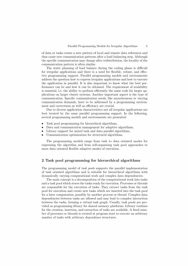
Load balancing and mapping of tasks is achieved automatically since aprocess extracts a task whenever processor time is available. There are sev-eral possibilities for the internal realization of task pools, which affect loadbalancing. Often the tasks are kept in task queues, see also Fig. 1:
• Central task pools: All tasks of the algorithm are kept in one task queuefrom which all threads extract tasks for execution and into which thenewly created tasks are inserted. Access conflicts are avoided by a lockmechanism for shared memory programming.
• Decentralized task pools: Each thread has its own task queue from whichthe thread extracts tasks and into which it inserts newly created tasks. Noaccess conflicts can occur and so there is no need for a lock mechanism. Butload imbalances can occur for irregularly growing computational work.
• Decentralized task pools with task stealing: This variant of the decentral-ized task pool offers a task stealing mechanism. Threads with an emptytask queue can steal tasks from other queues. Load imbalance is avoidedbut task stealing needs a locking mechanism for correct functionality.
P3P2P1P1 P3P2P1P1 P1P1 P3P2
Tasks Tasks
DecentralizedTask Pool
CentralTask Pool
ProcessorsTask-Stealin
g
Tasks
Fig. 1. Different types of task pool variants for shared memory
Due to the additional overhead of task pools it is suggested to use themonly when required for highly irregular and dynamic algorithms. Examples arethe hierarchical radiosity method from computer graphics and hierarchical n-body algorithms.
The hierarchical radiosity method
The radiosity algorithm is an observer-independent global illumination methodfrom computer graphics to simulate diffuse light in three-dimensional scenes[10]. The method is based on the energy radiation between surfaces of objectsand accounts for direct illumination and multiple reflections between surfaceswithin the environment. The radiosity method decomposes the surface of ob-jects in the scene into small elements Aj , j = 1, . . . , n, with almost constantradiation energy. For each element, the radiation energy is represented by aradiosity value Bj (of dimension [Watt/m2]) describing the radiant energy perunit time and per unit area dAj of Aj . The radiosity values of the elements
Parallel Programming Models for Irregular Algorithms 7
B F
ρ B
AE
A
A F
i i i ij
ji i i ij
j j
incident light
reflected light
emission of light
surface element
j
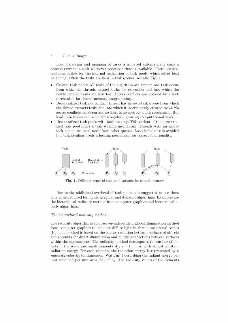
Fig. 2. Illustration of the radiosity equation
are determined by solving a linear equation system relating the different ra-diation energies of the scene using configuration factors (which express thegeometrical positioning of the elements), see also Fig. 2:
BjAj = EjAj + ρj
n∑
i=1
FijBiAi, j = 1, . . . , n. (1)
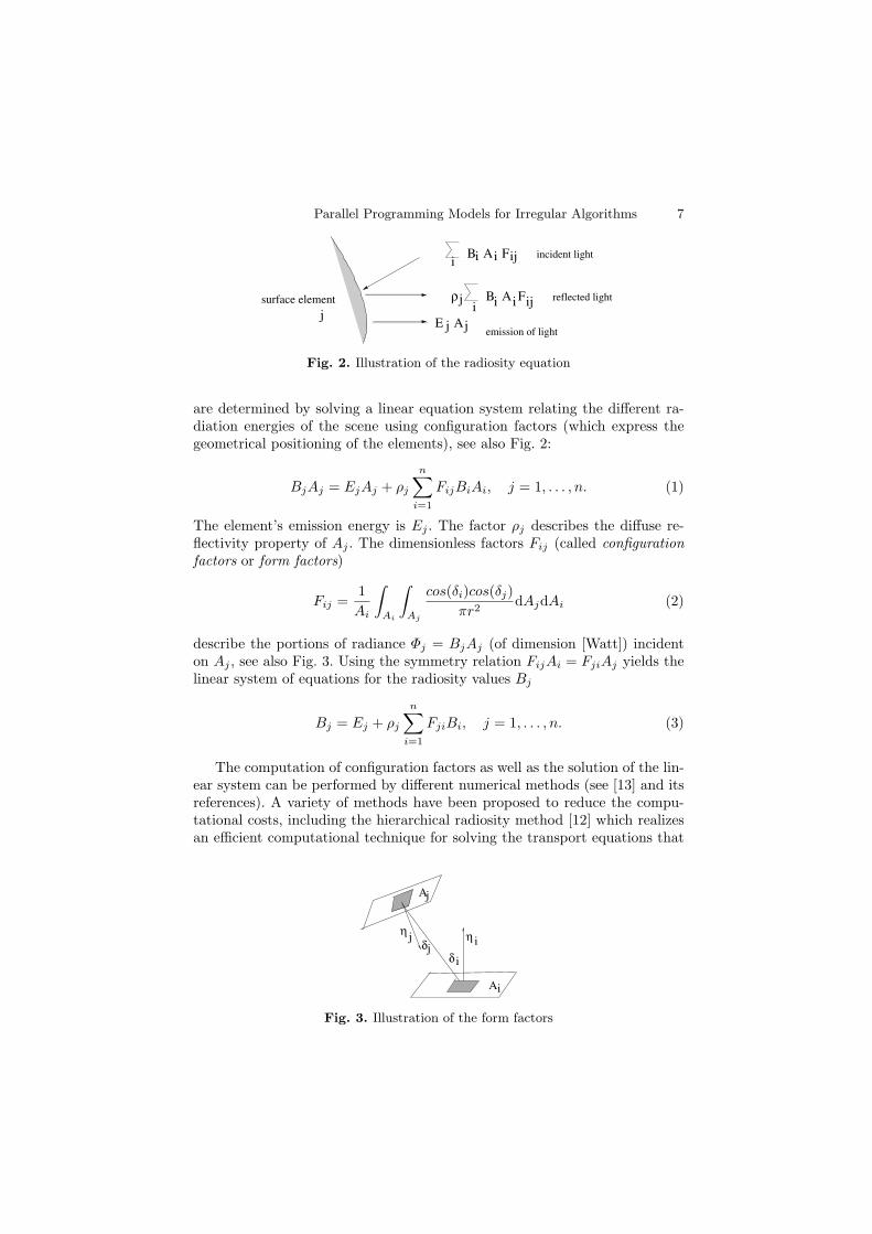
The element’s emission energy is Ej . The factor ρj describes the diffuse re-flectivity property of Aj . The dimensionless factors Fij (called configurationfactors or form factors)
Fij =1
Ai
∫
Ai
∫
Aj
cos(δi)cos(δj)
πr2dAjdAi (2)
describe the portions of radiance Φj = BjAj (of dimension [Watt]) incidenton Aj , see also Fig. 3. Using the symmetry relation FijAi = FjiAj yields thelinear system of equations for the radiosity values Bj
Bj = Ej + ρj
n∑
i=1
FjiBi, j = 1, . . . , n. (3)
The computation of configuration factors as well as the solution of the lin-ear system can be performed by different numerical methods (see [13] and itsreferences). A variety of methods have been proposed to reduce the compu-tational costs, including the hierarchical radiosity method [12] which realizesan efficient computational technique for solving the transport equations that
jA
Ai
η jδj
δ i
η i
Fig. 3. Illustration of the form factors
8 Gudula Runger
specify the radiosity values of surface patches in complex scenes. The mutualillumination of surfaces is computed more precisely for nearby surfaces andless precisely for distant surfaces.
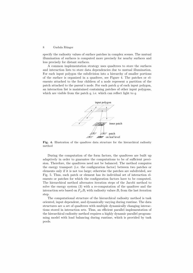
A common implementation strategy uses quadtrees to store the surfacesand interaction lists to store data dependencies due to mutual illumination.For each input polygon the subdivision into a hierarchy of smaller portionsof the surface is organized in a quadtree, see Figure 4. The patches or el-ements attached to the four children of a node represent a partition of thepatch attached to the parent’s node. For each patch q of each input polygon,an interaction list is maintained containing patches of other input polygons,which are visible from the patch q, i.e. which can reflect light to q.
input polygon
inner patch
patchon leaf level
Fig. 4. Illustration of the quadtree data structure for the hierarchical radiositymethod
During the computation of the form factors, the quadtrees are built upadaptively in order to guarantee the computations to be of sufficient preci-sion. Therefore, the quadtrees need not be balanced. The method computesthe energy transport (i.e. the configuration factor) between two patches orelements only if it is not too large; otherwise the patches are subdivided, seeFig. 5. Thus, each patch or element has its individual set of interaction el-ements or patches for which the configuration factors have to be computed.The hierarchical method alternates iteration steps of the Jacobi method tosolve the energy system (3) with a re-computation of the quadtree and theinteraction sets based on FjiBi with radiosity values Bi from the last iterationstep.
The computational structure of the hierarchical radiosity method is taskoriented, input dependent, and dynamically varying during runtime. The datastructures are a set of quadtrees with multiple dynamically changing interac-tions stored in interaction sets. Thus, an efficient parallel implementation ofthe hierarchical radiosity method requires a highly dynamic parallel program-ming model with load balancing during runtime, which is provided by taskpools.

Parallel Programming Models for Irregular Algorithms 9
quadtree of quadtree of
polygon A polygon B
p
I(p)
deleted
inserted
q
For all patches in the interaction set q I(p) area(p) > area(q)with
Fig. 5. Energy-based subdivision of a patch p and corresponding changes of inter-action lists I(p) in the hierarchical radiosity method
Extensive work concerning task pool implementations of hierarchical al-gorithms has been presented in [44]. How to realize a large potential of par-allelism with the task pool approach in order to employ a large number ofprocesses is investigated in [29]. In [27] additional task pool variants are pre-sented and their performance impact is investigated for different irregularapplications.
Task pool teams
For use on parallel platforms with distributed memory or on clusters, theidea of task pools has to be extended in order to include communication.One approach are task pool teams which combine task pools running on singlecluster nodes with explicit communication [15, 19]. To support complex taskand dependence structures in a dynamically growing task graph, a powerfulcommunication mechanism with asynchronous and dynamic communicationbetween tasks is needed. Asynchronous communication is required since itis not known in advance when and where a communication partner may beready for execution. Dynamic communication is required since it is impossibleto know in advance that a communication, e.g. for providing data, is requestedby another task.
Task pool teams for an SMP (symmetric multiprocessor) cluster combinesthread based task pools on SMP nodes with specific communication protocolshandling the communication requirements mentioned above. The realizationuses Pthreads for SMPs and MPI for communication between SMP nodes [11].A number of worker threads and one specific communication thread run oneach SMP node; the communication protocol for task pool teams supportsasynchronous communication between SMP nodes exploiting the communi-cation thread. For the application programmer, the programming supportprovides library routines for explicitly creating and extracting tasks; commu-nication patterns are also explicitly inserted in the parallel program.
10 Gudula Runger
The hierarchical radiosity method is one of the most challenging prob-lems concerning irregularity of data access and dynamic behavior of load andcommunication. Communication is required for remote data access as well asfor load balancing between nodes. Task pool teams provide an appropriatetool for handling load imbalances on SMP nodes as well as on entire clus-ter platforms. Load balance between SMP nodes is realized explicitly offeringadditional possibilities for optimizing the expensive redistribution of data ormigration of tasks.
The programming model of task pool teams also has been used to realizedifferent parallel variants of the simulation of diffusion processes using ran-dom Sierpinski Carpets [9,20]. In this application the task pool team approachis especially suitable to efficiently realize the boundary update phase of thealgorithm which is necessary after time steps. The first variant has a synchro-nous parallel update phase which exploits the specific communication threadprovided by task pool teams; the exchange of boundary information is startedby collective communication of the worker threads and the communicationthread is responsible for the processing of the data received. The second im-plementation variant realizes an asynchronous boundary-update using onlythe task pool team’s communication mechanism. Measurements of the exe-cution time on a Xeon-Cluster with SCI network and a Beowulf cluster withFast-Ethernet show that the synchronous approach is slightly better.
The central aim of using task pool teams is to support communicationprotocols that are suitable for dynamic and asynchronous communication,but which do not rely on specific attributes of the MPI library such as threadsafety [17]. Thus, the implementation provides great flexibility concerning theunderlying communication libraries, the parallel platform used, and specificapplication algorithms.
3 Data and communication managementfor adaptive algorithms
Adaptive algorithms adjust their behavior according to the specified proper-ties of the result to be computed. This includes an adaption of computationand/or data and is usual guided by a required precision of a solution. A typicalexample is the adaptive finite element method for solving partial differentialequations numerically.
The finite element method uses a discretization of the physical space intoa mesh of finite elements. The numerical solution of the given problem isthen computed iteratively on the mesh. The resulting numerical algorithmhas mainly local dependencies since only values stored for neighboring meshcells are used for the computation. Because of these local dependencies, auseful parallel implementation strategy exploits a decomposition of the meshinto parts of equal size in order to obtain load balance [3]. Communication is
Parallel Programming Models for Irregular Algorithms 11
minimized by using a decomposition into blocks with small boundaries suchthat a small amount of data is exchanged with the neighboring processors.
The adaptive finite element method starts with a coarse mesh and per-forms a stepwise refinement of the mesh according to the requested precisionof the approximation solution. From the mathematical point of view, errorestimation is an important point to guide the refinement. From the imple-mentation point of view, the appropriate data structures implementing themesh and an effective realization of the refinement is crucial. Treelike datastructures for storing the adaptive mesh and its refinement structures are oneoption.
For a parallel implementation, one has to deal with dynamically grow-ing or shrinking data structures during runtime and varying communicationneeds. However, there is a difference compared to the hierarchical algorithmintroduced in Sect. 2. The data dependencies of the finite element methodare local in the sense that data exchange is required only with neighboringmesh cells. This property still holds for the adaptive method. Neighboringmesh cells might be refined into several new mesh cells but the new neighborsfor communication are immediately known. No further unknown interactionoccurs. Thus, an appropriate parallel programming model for the adaptivefinite element method is a dynamic use of load balancing methods by graphpartitioning methods known from the non-adaptive case. Graph partitioningmethods can be used during runtime to achieve load balance.
Graph partitioning
The decomposition of data meshes is more complicated in the irregular caseand is related to the NP-hard graph partitioning problem which partitions agiven graph into subgraphs of almost equal size while cutting a minimal num-ber of edges. Graph partitioning algorithms use one- and multi-dimensionalpartitioning or recursive bisection [7, 30]. Recursive bisection includes thepartitioning according to coordinate values which is especially suitable forsparse matrices [46], recursive graph bisection exploiting local properties ofthe graph [26], or recursive spectral bisection using eigenvalues of the adja-cency matrix as global property [31]. Multi-level algorithms for graph parti-tioning use multiple levels of the graph with different refinement which areproduced in sequence of consecutive steps [14, 23, 24]. Programming supportfor the partitioning of unstructured graphs or reordering of sparse matrices isprovided by the METIS System [22,25].
The execution time for graph partitioning algorithms adds an additionaloverhead to the parallel execution time of the application problem to be solved,since the graph partitioning and repartitioning have to be done at runtime.The resulting communication time can be very high such that the incorpora-tion of repartitioning may result in a more expensive parallel program. Thus,irregular algorithms with dynamically varying data structures usually requirean additional mechanism for an efficient implementation.
12 Gudula Runger
Data and communication management for adaptive finite element methods
The efficient parallel implementation of a hexahedral adaptive finite elementmethod has been presented in [16]. In this approach, the communication isencapsulated in order to provide a general mechanism for repartitioning ingraph based algorithms.
The main characteristics inducing irregularity to adaptive hexahedral FEMare adaptively refined data structures and hanging nodes. A hanging node isa vertex of an element that can be a mid node of a face or an edge. Suchnodes can occur when hexahedral elements are refined irregularly, i.e. whenneighboring volumes have different levels of refinement. For a correct numer-ical computation, hanging nodes require projections onto nodes of other re-finement levels during the solution process. The adaptive refinement processwith computations on different refinement levels creates hierarchies of datastructures and requires the explicit storage of these structures including theirrelations. These characteristics lead to irregular communication behavior andload imbalances in a parallel program.
The task pool team approach from Sect. 2 provides a concept which allowsany kind of data references or communication patterns, including strong ir-regular communication. For adaptive FEM, however, the locality of referencesand communication is slightly different than described for the algorithms pre-sented in the last section.
• The adaptive FEM has a data oriented program structure with dynam-ically growing (or shrinking) data structures. Based on the input data asuitable initial distribution of data can be chosen at program start.
• The computational effort varies dynamically according to the dynamicbehavior of the data. The process is guided by the FEM algorithm withappropriate error estimation methods.
• The data dependencies are of local character, i.e. there are dependencies toneighboring cells in the mesh or graph data structures. This leads to localcommunication patterns in a parallel program with only a few neighboringprocessors.
• For efficient parallel execution, load redistribution is required during run-time. But load increases resulting from adaptive refinement are usuallyconcentrated on a few processors. Appropriate load redistribution may af-fect all processors but are of local nature between neighboring processors.
• Communication occurs for remote data access when data are needed forcalculation. Also shared data structures have to be maintained consistentlyduring program run. In most cases the exact time of communication isnot known in advance. Message sizes or communication partners vary anddepend on the input. However, the communication partners work synchro-nously.
A parallel FEM implementation can exploit the locality of references andlocal communication pattern. A suitable data management and communica-tion layer for adaptive three-dimensional hexahedral FEM is presented in [18].
Parallel Programming Models for Irregular Algorithms 13
The data management assumes a distribution of volumes across the proces-sors where neighboring volumes share faces, edges, or nodes of the mesh datastructure. The mapping of neighboring volumes to different processors requiresan appropriate storage of those shared data such that the data managementguarantees correct storage and a correct access to the data. The following datastructures have been proposed:
• Shared data are stored as duplicates in all processors holding parts of thecorresponding volumes. The solution vector is distributed correspondingly.Specific restrictions guarantee the correct computation on those data.
• The data structure and its distribution are refined consistently in two steps:a local refinement step for data which are only kept in the memory of onespecific processor and a remote refinement step for data with duplicatesin the memories of other processors.
• Coherence lists store the information about the distribution of data tosupport remote refinement and fast identification of communication part-ners. Due to the locality properties of adaptive FEM the remote refinementapplies to neighboring processors.
The communication layer provides support for different communicationsituations that can occur in adaptive FEM:
• Synchronization and exchange of results between neighboring processorsduring the computation step.
• Accumulation of local subtotals which yield the total result after a com-putation step.
• Exchange of administration information after a refinement of volumes,including remote refinement, creation or update of duplicate lists, andidentification of hanging nodes.
The second and third communication situations are of irregular type andare handled with a specific protocol. This protocol deals with asynchronouscommunication since the exact moment of communication is unknown andcan take place with varying communication partners and message sizes. Acollection phase gathers information about remote duplicates and its ownersneeded for the communication. Additionally, each processor asynchronouslyprovides information about duplicate data requested by other processors inthe collection phase.
A suitable method for repartitioning and load balancing is the use of agraph partitioning tools like ParMetis. The communication protocol presentedin [18] can be combined with graph partitioning and guarantees the correctbehavior after each repartitioning. The protocol has been used for the paral-lelization of the program version SPC-PM3AdH which realizes a 3-dimensionaladaptive hexahedral FEM method suitable to solve elliptic partial differentialequations [2]. The parallelization method can be applied to all adaptive algo-rithms which provide similar locality properties and similar communicationpatterns as adaptive FEM codes.
14 Gudula Runger
4 Library support for mixed taskand data parallel algorithms
A large variety of application problems from scientific computing and relatedareas have an inherent modular structure of cooperating subtasks calling eachother. Examples include environmental models combining atmospheric, sur-face water, and ground water models, as well as aircraft simulations combiningmodels for fluid dynamics, structural mechanics, and surface heating, see [1]for an overview. But modular structures can also be found within numerical al-gorithms built up from submethods. For the efficient parallel implementationof those applications an appropriate parallel programming model is neededwhich can express a (hierarchical) modular structure.
The SPMD (single program multiple data) model proposed in [5] was fromits inception more general than a data parallel model and did allow a hierar-chical expression of parallelism, however most implementations exploit only adata parallel form. But many research groups have proposed models for mixedtask and data parallel executions with the goal of obtaining parallel programswith faster execution time and better scalability properties, see [1, 45] for anoverview of systems and programming approaches and see [4] for a detailedinvestigation of the benefits of combining task and data parallel executions.Several models support the programmer in writing efficient parallel programsfor modular applications without dealing too much with the underlying com-munication and coordination details of a specific parallel machine. Languageapproaches include Braid, Fortran M, Fx, Opus, and Orca, see [1]. FortranM [8] allows the creation of processes which can communicate with each otherby predefined channels and which can be combined with HPF Fortran for amixed task and data parallel execution.
The TwoL (Two Level) model uses a stepwise transformation approachfor creating an efficient parallel program from a module specification of thealgorithm (upper level) with calls to basic modules (lower level) [34, 36]. Thetransformation approach can be realized by a compiler tool and is suitablefor statically known module structures. Different recent realizations of thespecification mechanism have been proposed in [28] and [41]. For dynamicallygrowing and varying modular structures, however, support at runtime is re-quired which is provided by the runtime library Tlib for multiprocessor taskprogramming.
Multiprocessor task programming
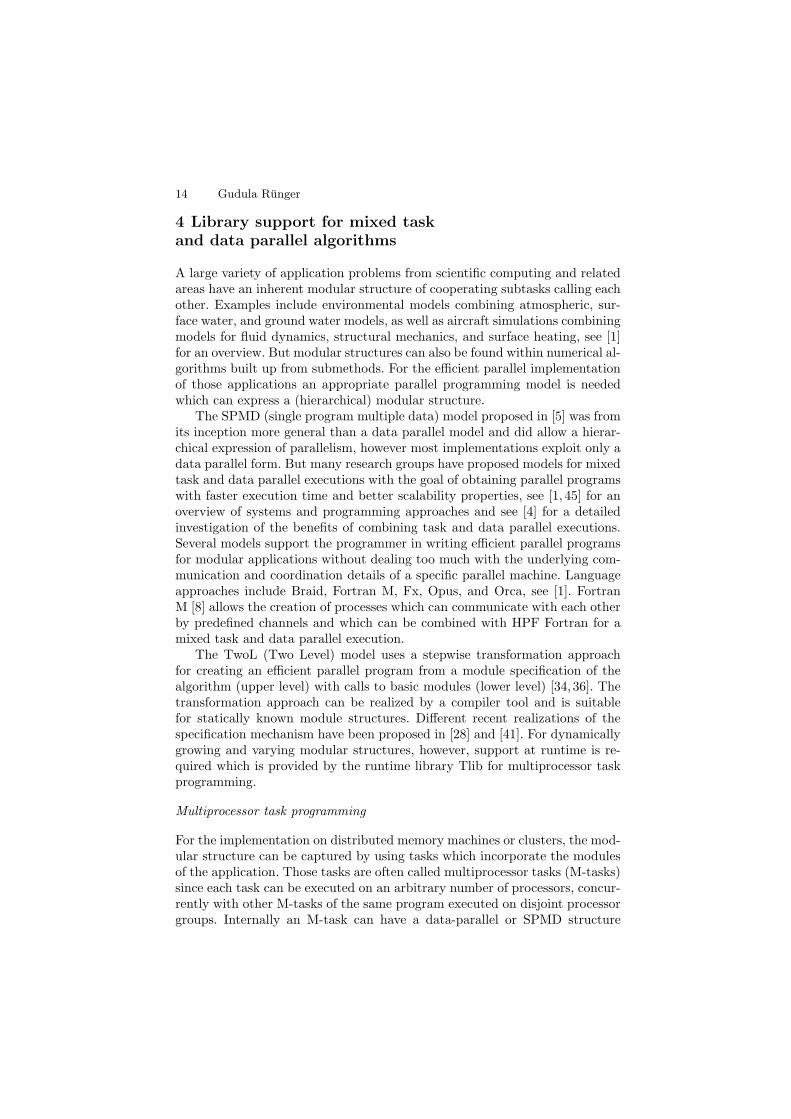
For the implementation on distributed memory machines or clusters, the mod-ular structure can be captured by using tasks which incorporate the modulesof the application. Those tasks are often called multiprocessor tasks (M-tasks)since each task can be executed on an arbitrary number of processors, concur-rently with other M-tasks of the same program executed on disjoint processorgroups. Internally an M-task can have a data-parallel or SPMD structure
Parallel Programming Models for Irregular Algorithms 15
but may also have an internal hierarchical and modular structure. The entireM-task program consists of a set of cooperating, hierarchically structured M-tasks which mimic the module dependence structure of the algorithm. M-taskprogramming can be used to design parallel programs with mixed task anddata parallelism where a coarse structure of tasks form a coarse-grained hier-archical M-task graph, see Fig. 6. The execution mode is group-SPMD whereat each point in execution time disjoint processor groups execute separateSPMD modules of the algorithm.
M−Taskdata parallel or SPMD
independent
M−Task
Communication
data dependency
Fig. 6. Illustration of an M-task graph and its potential parallelism. Nodes denoteM-tasks and arrows denote data dependencies between tasks which might result incommunication
The advantage of the described form of mixed task and data parallelismis a potential for reducing the communication overhead and for improvingscalability, especially if collective communication operations are used. Collec-tive communication operations performed on smaller processor groups lead tosmaller execution times due to the logarithmic or linear dependence of thecommunication times on the number of processors [38,48]. As a consequence,the concurrent execution of independent tasks on disjoint processor subsets ofappropriate size can result in smaller parallel execution times than the con-secutive execution of the same M-tasks one after another on the entire set ofprocessors.
Modular structures can be found in many numerical algorithms of multi-level form [21]. As an example we describe the potential of M-task parallelismin solution methods for ordinary differential equations.
Modular structures of Runge-Kutta methods
Numerical methods for solving systems of ordinary differential equations ex-hibit a nested or hierarchical structure which makes them amenable to a mixedtask and data parallel realization. An example is the diagonal-implicitly it-erated Runge-Kutta (DIIRK) method which is an implicit solution methodwith integrated step-size and error control for ordinary differential equations
16 Gudula Runger
ComputeStageVectors
InitializeStage
StepsizeControl
ComputeApprox
NewtonIter
SolveLinSyst
NewtonIter
SolveLinSyst
Initialization
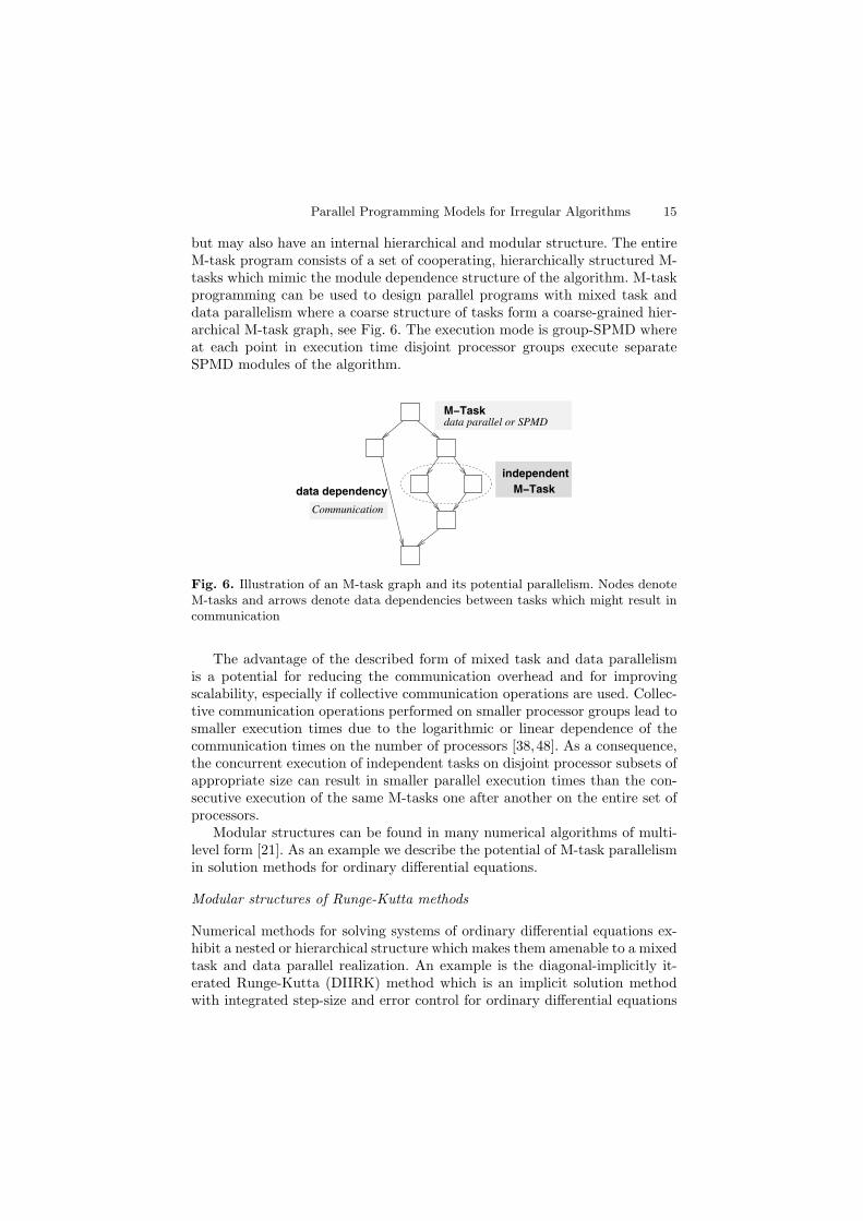
Fig. 7. Illustration of the modular structure of the diagonal-implicitly iteratedRunge-Kutta method
(ODEs) arising, e.g., when solving time-dependent partial differential equa-tions with the method of lines [47].
The modular structure of this solver is given in Figure 7 where boxes denoteM-tasks and back arrows denote loop structures. In each time step, the solvercomputes a fixed number of s stage vectors (ComputeStageVectors) which arethen combined to the final approximation (ComputeApprox). The methodoffers a potential of parallel execution of M-tasks since the computation ofthe different stage vectors are independent of each other [35]. Each singlecomputation of a stage vector requires the solution of a non-linear equationsystem whose size is determined by the system size of the ordinary differentialequations. The non-linear systems are solved with a modified Newton method(NewtonIter) requiring the solution of a linear equation system (SolveLinSyst)in each iteration step. Depending on the characteristics of the linear systemand the solution method used, a further internal mixed task and data parallelexecution can be used, leading to another level in the task hierarchy. A parallelimplementation can exploit the modular structure in several different waysbut can also execute the entire method in a pure SPMD fashion. The differentimplementations differ in the coordination of the M-tasks and usually differin the resulting parallel execution time.
Runtime library Tlib
The runtime library Tlib supports M-task programming with varying, hi-erarchically structured, recursive M-tasks cooperating according to a givencoordination program [39]. The coordination program contains activations ofcoordination operations of the Tlib library and user-defined M-task functions.

Parallel Programming Models for Irregular Algorithms 17
The parallel programming model for Tlib programs is a group-SPMD modelat each point in the execution time. This results in a multilevel group-SPMDmodel with several different hierarchies of processor groups due to the dynamicchange of processor groups during runtime and nested M-task calls.
Tlib mainly provides two kinds of operations:
• a family of split operations to structure the given set of processors and• a family of mapping operations to assign specific M-tasks to specific proces-
sor groups for execution.
M-tasks cooperate through parameters which can include composed datastructures so that Tlib programs have to deal with data placement, datadistribution, and data redistribution. The specific challenge for selecting adata distribution lies in the dynamic character of M-task programs in Tlib,since the actual M-task structure and the processor layout are not necessarilyknown in advance. The advantage of this dynamic behavior is that arbitrary,hierarchically structured and recursive M-task programs can be coded easily,providing an easy way to express divide-and-conquer algorithms or irregularalgorithms. For a data distribution and a correct cooperation of arbitrary M-tasks a specific data format is needed which fits the dynamic needs of themodel [40].
5 Communication optimization for structured algorithms
The locality of dependencies can also be exploited to optimize the communi-cation for parallel algorithms with a more structured data or task dependencegraph. The parallel programming model of orthogonal processor groups pro-vides a group-SPMD model for applications with a two- or higher-dimensionaldata or task grid where dependencies are mainly aligned in the dimensionsof this grid. The advantage is a reduction of the communication to smallergroups of processors which leads to a reduction of the communication over-head as already mentioned in Sect. 4. The entire set of processors executingan application program is organized in a virtual two- or higher-dimensionalprocessor grid and a fixed number of different decompositions of this set intodisjoint processor subsets is defined. The subsets of a decomposition into dis-joint processor groups correspond to the lower-dimensional hyperplanes of thevirtual processor grid which are geometrically orthogonal to each other.
An application algorithm is mapped onto the processor grid according toits natural grid based data or task structure. The program executes a sequenceof phases in which a processor alternatively executes the tasks assigned to itin an SPMD or group-SPMD way. In a group-SPMD phase the applicationprogram uses exactly one of the decompositions into processor hyperplanesand a processor within a hyperplane performs an SPMD computation togetherwith other processors in the same group, including group internal collective
18 Gudula Runger
communication operations. At each time of the execution only one partitioncan be active.
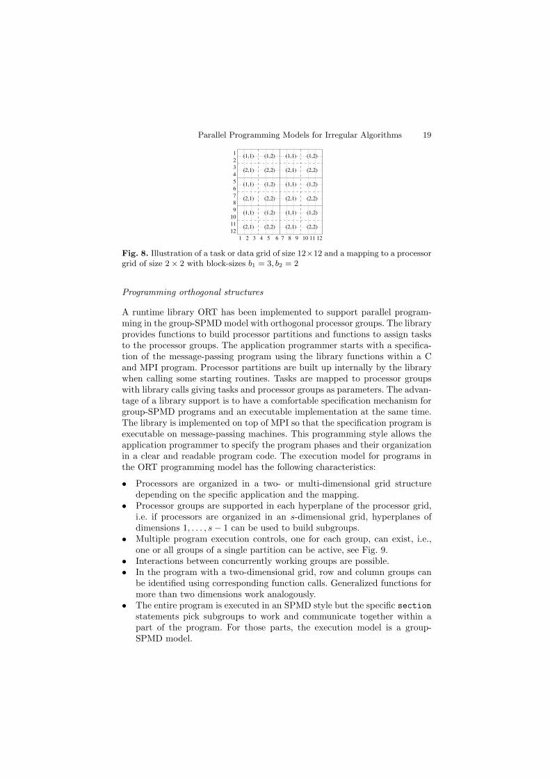
For programming with virtual processor grids, a suitable coding of proces-sor grids and grid based data or task structures is needed. Parameterized dataor task distributions can be used as a flexible technique for the mapping ofdata or tasks to processor subgroups.
Parameterized data or task mapping
Parameterized data distributions describe the data distribution for data gridsof arbitrary dimension [6,37]. A task is assigned to exactly one processor, buteach processor might have several tasks assigned to it.
A parameterized cyclic mapping of a d-dimensional task grid to a virtualprocessor grid of size p1 × · · · × pd is specified by a block-size bl, l = 1, . . . , d,in each dimension l. The block-size bl determines the number of consecutiveelements that each processor obtains from each cyclic block in this dimension.For a total number of p processors, the distribution of the data or task gridT of size n1 × · · · × nd is described by an assignment vector of the form:
((p1, b1), . . . , (pd, bd)) (4)
with p =∏d
l=1 pl and 1 ≤ bl ≤ nl for l = 1, . . . , d. For simplicity we assumenl/(pl · bl) ∈ N.
The set of processors is divided into disjoint subsets of processors due tothe virtual d-dimensional processor number in a d-dimensional processor grid.For the two-dimensional processor grid of size p1 × p2, there are two differentdecompositions into a disjoint set of p2 row groups Rq, 1 ≤ q ≤ p2, and intoa disjoint set of p1 column groups Cq, 1 ≤ q ≤ p1:
Rq = (r, q) | r = 1, . . . , p1 , Cq = (q, r) | r = 1, . . . , p2 (5)
with |Rq| = p1 and |Cq| = p2. The row and column groups build separateorthogonal partitions of the set of processors P , i.e.,
p2⋃
q=1
Rq =
p1⋃
q=1
Cq = P and Rq ∩Rq′ = ∅ = Cq ∩ Cq′ for q = q′.
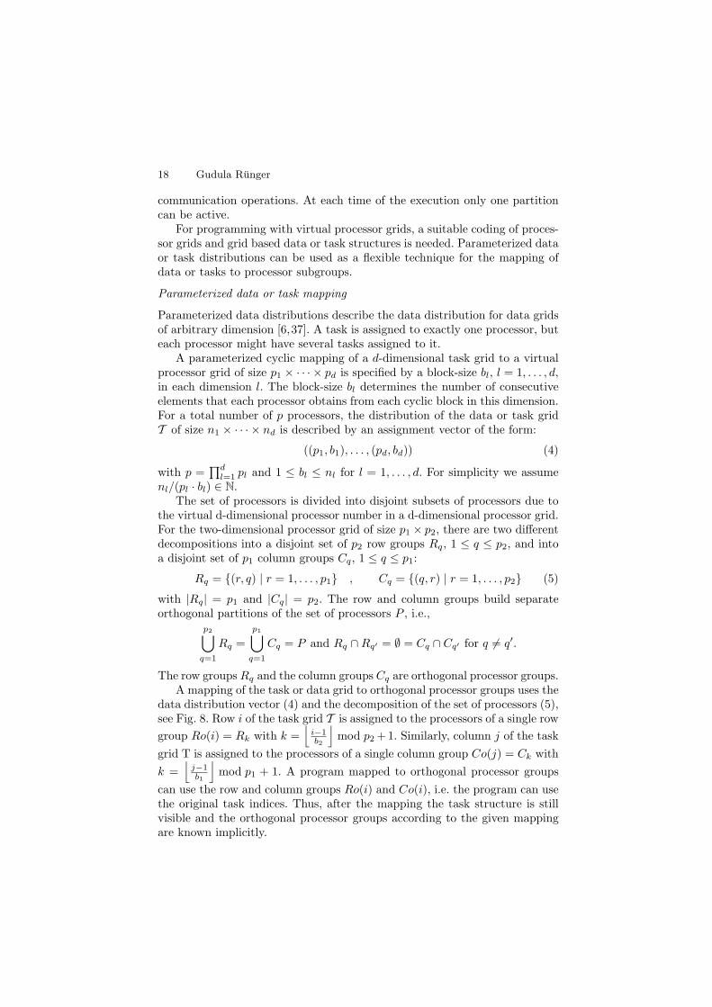
The row groupsRq and the column groups Cq are orthogonal processor groups.A mapping of the task or data grid to orthogonal processor groups uses the
data distribution vector (4) and the decomposition of the set of processors (5),see Fig. 8. Row i of the task grid T is assigned to the processors of a single row
group Ro(i) = Rk with k =⌊
i−1b2
⌋mod p2 +1. Similarly, column j of the task
grid T is assigned to the processors of a single column group Co(j) = Ck with
k =⌊
j−1b1
⌋mod p1 + 1. A program mapped to orthogonal processor groups
can use the row and column groups Ro(i) and Co(i), i.e. the program can usethe original task indices. Thus, after the mapping the task structure is stillvisible and the orthogonal processor groups according to the given mappingare known implicitly.
Parallel Programming Models for Irregular Algorithms 19
1
2
3
4
5
6
7
8
9
10
11
12
1 2 3 4 5 6 7 8 9 10 11 12
(1,1) (1,2) (1,1) (1,2)
(2,1) (2,2) (2,1) (2,2)
(1,1)
(2,1)
(1,2)
(2,2)
(1,1)
(2,1)
(1,2)
(2,2)
(1,1)
(2,1)
(1,2)
(2,2)
(1,1)
(2,1)
(1,2)
(2,2)
Fig. 8. Illustration of a task or data grid of size 12×12 and a mapping to a processorgrid of size 2 × 2 with block-sizes b1 = 3, b2 = 2
Programming orthogonal structures
A runtime library ORT has been implemented to support parallel program-ming in the group-SPMD model with orthogonal processor groups. The libraryprovides functions to build processor partitions and functions to assign tasksto the processor groups. The application programmer starts with a specifica-tion of the message-passing program using the library functions within a Cand MPI program. Processor partitions are built up internally by the librarywhen calling some starting routines. Tasks are mapped to processor groupswith library calls giving tasks and processor groups as parameters. The advan-tage of a library support is to have a comfortable specification mechanism forgroup-SPMD programs and an executable implementation at the same time.The library is implemented on top of MPI so that the specification program isexecutable on message-passing machines. This programming style allows theapplication programmer to specify the program phases and their organizationin a clear and readable program code. The execution model for programs inthe ORT programming model has the following characteristics:
• Processors are organized in a two- or multi-dimensional grid structuredepending on the specific application and the mapping.
• Processor groups are supported in each hyperplane of the processor grid,i.e. if processors are organized in an s-dimensional grid, hyperplanes ofdimensions 1, . . . , s− 1 can be used to build subgroups.
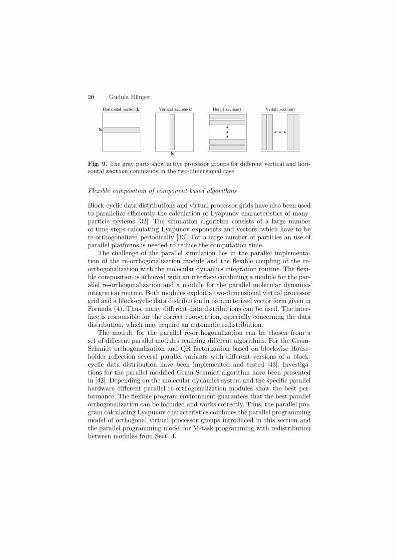
• Multiple program execution controls, one for each group, can exist, i.e.,one or all groups of a single partition can be active, see Fig. 9.
• Interactions between concurrently working groups are possible.• In the program with a two-dimensional grid, row and column groups can
be identified using corresponding function calls. Generalized functions formore than two dimensions work analogously.
• The entire program is executed in an SPMD style but the specific sectionstatements pick subgroups to work and communicate together within apart of the program. For those parts, the execution model is a group-SPMD model.
20 Gudula Runger
k
k
Vertall_section()Horall_section()Vertical_section(k)Horizontal_section(k)
Fig. 9. The gray parts show active processor groups for different vertical and hori-zontal section commands in the two-dimensional case
Flexible composition of component based algorithms
Block-cyclic data distributions and virtual processor grids have also been usedto parallelize efficiently the calculation of Lyapunov characteristics of many-particle systems [32]. The simulation algorithm consists of a large numberof time steps calculating Lyapunov exponents and vectors, which have to bere-orthogonalized periodically [33]. For a large number of particles an use ofparallel platforms is needed to reduce the computation time.
The challenge of the parallel simulation lies in the parallel implementa-tion of the re-orthogonalization module and the flexible coupling of the re-orthogonalization with the molecular dynamics integration routine. The flexi-ble composition is achieved with an interface combining a module for the par-allel re-orthogonalization and a module for the parallel molecular dynamicsintegration routine. Both modules exploit a two-dimensional virtual processorgrid and a block-cyclic data distribution in parameterized vector form given inFormula (4). Thus, many different data distributions can be used. The inter-face is responsible for the correct cooperation, especially concerning the datadistribution, which may require an automatic redistribution.
The module for the parallel re-orthogonalization can be chosen from aset of different parallel modules realizing different algorithms. For the Gram-Schmidt orthogonalization and QR factorization based on blockwise House-holder reflection several parallel variants with different versions of a block-cyclic data distribution have been implemented and tested [43]. Investiga-tions for the parallel modified Gram-Schmidt algorithm have been presentedin [42]. Depending on the molecular dynamics system and the specific parallelhardware different parallel re-orthogonalization modules show the best per-formance. The flexible program environment guarantees that the best parallelorthogonalization can be included and works correctly. Thus, the parallel pro-gram calculating Lyapunov characteristics combines the parallel programmingmodel of orthogonal virtual processor groups introduced in this section andthe parallel programming model for M-task programming with redistributionbetween modules from Sect. 4.
Parallel Programming Models for Irregular Algorithms 21
References
1. H. Bal and M. Haines. Approaches for Integrating Task and Data Parallelism.IEEE Concurrency, 6(3):74–84, July-August 1998.
2. S. Beuchler and A. Meyer. SPC-PM3AdH v1.0, Programmer’s Manual. Techni-cal Report SFB393/01-08, Chemnitz University of Technology, 2001.
3. W. J. Camp, S. J. Plimpton, B. A. Hendrickson, and R. W. Leland. MassivelyParallel Methods for Engineering and Science Problems. Comm. of the ACM,37:31–41, 1994.
4. S. Chakrabarti, J. Demmel, and K. Yelick. Modeling the benefits of mixed dataand task parallelism. In Symposium on Parallel Algorithms and Architecture(SPAA), pages 74–83, 1995.
5. F. Darema, D. A. George, V. A. Norton, and G. F. Pfister. A single-program-multiple-data computational mode for EPEX/FORTRAN. Parallel Comput.,7(1):11–24, 1988.
6. A. Dierstein, R. Hayer, and T. Rauber. The addap system on the ipsc/860:Automatic data distribution and parallelization. J. Parallel Distrib. Comput.,32(1):1–10, 1996.
7. U. Elsner. Graph Partitioning. Technical Report SFB 393/97 27, TU Chemnitz,Chemnitz, Germany, 1997.
8. I. Foster and K.M. Chandy. Fortran M: A Language for Modular Parallel Pro-gramming. J. Parallel Distrib.Comput., 25(1):24–35, April 1995.
9. A. Franz, C. Schulzky, S. Seeger, and K.H. Hoffmann. An efficient implementa-tion of the exact enumeration method for random walks on sierpinski carpets.Fractals, 8(2):155–161, 2000.
10. C.M. Goral, K.E. Torrance, D.P. Greenberg, and B. Battaile. Modeling theinteraction of light between diffuse surfaces. Computer Graphics, 18(3):212–222, 1984. Proceedings of the SIGGRAPH ’84.
11. W. Gropp, E. Lusk, and A. Skjellum. Using MPI: Portable Parallel Program-ming with the Message-Passing Interface. MIT Press, 1999.
12. P. Hanrahan, D. Salzman, and L.Aupperle. A rapid hierarchical radiosity algo-rithm. Computer Graphics, 25(4):197–206, 1991. Proceedings of SIGGRAPH’91.
13. P.S. Heckbert. Simulating Global Illumination using Adaptive Meshing. PhDthesis, University of California, Berkeley, 1991.
14. B. Hendrickson and R. Leland. A multi-level algorithm for partitioning graphs.In Proc. of the ACM/IEEE Conf. on Supercomputing, San Diego, USA, 1995.
15. J. Hippold. Dezentrale Taskpools auf Rechnern mit verteiltem Speicher. Diplom-arbeit, TU Chemnitz, Fakultat fur Informatik, Dezember 2001.
16. J. Hippold, A. Meyer, and G. Runger. A Parallelization Module for Adaptive3-Dimensional FEM on Distributed memory. In Proc. of the Int. Conferenceof Computational Science (ICCS-2004), LNCS 3037, pages 146–154. Springer,2004.
17. J. Hippold and G. Runger. A Communication API for Implementing IrregularAlgorithms on SMP Clusters. In J. Dongarra, D. Lafarenza, and S. Orlando,editors, Proc. of the 10th EuroPVM/MPI, volume 2840 of LNCS, pages 455–463,Venice, Italy, 2003. Springer.
18. J. Hippold and G. Runger. A Data Management and Communication Layer forAdaptive, Hexahedral FEM. In M. Danelutto, D. Laforenza, and M. Vanneschi,
22 Gudula Runger
editors, Proc. of Euro-Par 2004, volume 3149 of LNCS, pages 718–725, Pisa,Italy, 2004. Springer.
19. J. Hippold and G. Runger. Task Pool Teams: A Hybrid Programming Environ-ment for Irregular Algorithms on SMP Clusters. To appear: Concurrency andComputation: Practice and Experience, 2006.
20. M. Hofmann. Verwendung von Task Pool Teams Konzepten zur parallelen Im-plementierung von Diffusionsprozessen auf Fraktalen. Studienarbeit, TU Chem-nitz, Fakultat fur Informatik, Februar 2005.
21. S. Hunold, T. Rauber, and G. Runger. Multilevel Hierarchical Matrix Multipli-cation on Clusters. In Proc. of the 18th Annual ACM International Conferenceon Supercomputing, ICS’04, pages 136–145, June 2004.
22. G. Karypis and V. Kumar. METIS Unstructured Graph Partitioning and SparseMatrix Ordering System. Technical Report http://www.cs.umn.edu/metis, De-partment of Computer Science, University of Minnesota, Minneapolis, MN,USA, 1995.
23. G. Karypis and V. Kumar. Multilevel k-way Partitioning Scheme for IrregularGraphs. J. Parallel Distrib. Comput., 48:96–129, 1998.
24. G. Karypis and V. Kumar. A Fast and Highly Quality Multilevel Scheme forPartitioning Irregular Graphs. SIAM Journ. of Scientific Computing, 20(1):359–392, 1999.
25. G. Karypis, K. Schloegel, and V. Kumar. ParMETIS Parallel Graph Partitioningand Sparse Matrix Ordering Library, Version 3.0. Technical report, Universityof Minnesota, Department of Computer Science and Engineering, Army HPCResearch Center, Minneapolis, MN, USA, 2002.
26. B. Kernighan and S. Lin. An Efficient Heuristic Procedure for PartitioningGraphs. Bell System Technical Journ., 29:291–307, 1970.
27. M. Korch and T. Rauber. A Comparison of Task Pools for Dynamic LoadBalancing of Irregular Algorithms. Concurrency and Computation: Practiceand Experience, 16:1–47, 2004.
28. J. O’Donnell, T. Rauber, and G. Runger. Functional realization of coordinationenvironments for mixed parallelism. In Proc. of the IPDPS04 workshop onAdvances in Parallel and Distributed Computational Models, CD-ROM, SantaFe, New Mexico, USA, 2004. IEEE.
29. A. Podehl, T. Rauber, and G. Runger. A Shared-Memory Implementation ofthe Hierarchical Radiosity Method. Theoretical Computer Science, 196(1-2):215–240, 1998.
30. A. Pothen. Graph Partitioning Algorithms with Applications to Scientific Com-puting. In D. F. Keyws, A. H. Sameh, and V. Venkatakrishnan, editors, ParallelNumerical Algorithms. Kluwer, 1996.
31. A. Pothen, H. D. Simon, and K. P. Liou. Partitioning Sparse Matrices withEigenvectors of Graphs. SIAM Journ. on Matrix Analysis and Applications,11:430–452, 1990.
32. G. Radons, G. Runger, M. Schwind, and G. Yang. Parallel algorithms for thedetermination of Lyapunov characteristics of large nonlinear dynamical systems.In To appear: Proc. of PARA04 Workshop on State-of-the-Art in Scientific Com-puting 2004. Denmark, 2006.
33. G. Radons and H. L. Yang. Static and Dynamic Correlations in Many-ParticleLyapunov Vectors. nlin.CD/0404028, and references therein.
Parallel Programming Models for Irregular Algorithms 23
34. T. Rauber and G. Runger. The Compiler TwoL for the Design of Parallel Imple-mentations. In Proc. 4th Int. Conf. on Parallel Architectures and CompilationTechniques (PACT’96), IEEE, pages 292–301, 1996.
35. T. Rauber and G. Runger. Diagonal-Implicitly Iterated Runge-Kutta Meth-ods on Distributed Memory Machines. Int. Journal of High Speed Computing,10(2):185–207, 1999.
36. T. Rauber and G. Runger. A Transformation Approach to Derive Efficient Par-allel Implementations. IEEE Transactions on Software Engineering, 26(4):315–339, 2000.
37. T. Rauber and G. Runger. Deriving array distributions by optimization tech-niques. Journal of Supercomputing, 15:271–293, 2000.
38. T. Rauber and G. Runger. Modelling the runtime of scientific programs onparallel computers. In Y. Pan and L.T. Yang, editors, Parallel and DistributedScientific and Engineering Computing, volume 15 of Adv. in Computations: The-ory and Practice, pages 51–65. Nova Science Publ., 2004.
39. T. Rauber and G. Runger. Tlib - A Library to Support Programming withHierarchical Multi-Processor Tasks. J. Parallel Distrib. Comput., 65:347 – 360,2005.
40. T. Rauber and G. Runger. A data re-distribution library for multi-processor taskprogramming. To appear: International Journal of Foundations of ConmputerScience, 2006.
41. R. Reilein-Ruß. Eine komponentenbasierte Realisierung der TwoL-Sprach-architektur. Dissertation, TU Chemnitz, Fakultat fur Informatik, 2005.
42. G. Runger and M. Schwind. Comparison of different parallel modified gram-schmidt algorithm. In Proc. of Euro-Par 2005, LNCS, Lisboa, Portugal, 2005.Springer.
43. M. Schwind. Implementierung und Laufzeitevaluierung paralleler Algorithmenzur Gram-Schmidt Orthogonalisierung und zur QR-Zerlegung. Diplomarbeit,TU Chemnitz, Fakultat fur Informatik, Dezember 2004.
44. J.P. Singh, C. Holt, T. Totsuka, A. Gupta, and J. Hennessy. Load balancingand data locality in adaptive hierarchical N-body methods: Barnes-hut, fastmultipole, and radiosity. J. Parallel Distrib. Comput., 27:118–141, 1995.
45. D. Skillicorn and D. Talia. Models and languages for parallel computation. ACMComputing Surveys, 30(2):123–169, 1998.
46. M. Ujaldon, E. L. Zapata, S. D. Sharma, and J. Saltz. Parallelization Techniquesfor Sparse Matrix Applications. J. Parallel Distrib. Comput., 38(2):256–266,1996.
47. P.J. van der Houwen, B.P. Sommeijer, and W. Couzy. Embedded DiagonallyImplicit Runge–Kutta Algorithms on Parallel Computers. Mathematics of Com-putation, 58(197):135–159, January 1992.
48. Z. Xu and K. Hwang. Early Prediction of MPP Performance: SP2, T3D andParagon Experiences. Parallel Comput., 22:917–942, 1996.

Basic Approach to Parallel Finite ElementComputations: The DD Data Splitting
Arnd Meyer
Technische Universitat Chemnitz, Fakultat fur Mathematik09107 Chemnitz, [email protected]
1 Introduction
From Amdahl’s Law we know: the efficient use of parallel computers can notmean a parallelization of some single steps of a larger calculation, if in thesame time a relatively large amount of sequential work remains or if specialconvenient data structures for such a step have to be produced with the helpof expensive communications between the processors. From this reason, ourbasic work on parallel solving partial differential equations was directed toinvestigating and developing a natural fully parallel run of a finite elementcomputation – from parallel distribution and generating the mesh – over par-allel generating and assembling step – to parallel solution of the resulting largelinear systems of equation and post–processing.
So, we will define a suitable data partitioning of all large finite element(F.E.) data that permits a parallel use within all steps of the calculation.
This is given in detail in the following Sect. 2. Considering a typical it-eration method for solving a linear finite element system of equations, as isdone in Sect. 3, we conclude that the only relevant communication techniquehas to be introduced within the preconditioning step. All other parts of thecomputation show a purely local use of private data. This is important forboth message passing systems (local memory) and shared memory computersas well. The first environment clearly uses the advantage of having as lessinterprocessor communication as possible. But even in the shared memory en-vironment we obtain advantages from our data distribution. Here, the use ofprivate data within nearly all computational steps does not require any of thewell–known expensive semaphore–like mechanisms in order to secure writingconflicts. The same concept as in the distributed memory case permits theuse of the same code for both very different architectures.
26 Arnd Meyer
2 Finite element computation and data splitting
Leta(u, v) = 〈f, v〉 (1)
be the underlying bilinear form belonging to a partial differential equation(p.d.e.) Lu = f in Ω with boundary conditions as usual. Here, u ∈ H1(Ω)with prescribed values on parts ΓD of the boundary ∂Ω is the unknown so-lution, so (1) holds for all v ∈ H1
0 (Ω) (with zero values on ΓD). The FiniteElement Method defines an approximation uh of piecewise polynomial func-tions depending on a given fine triangulation of Ω.
Let Vh denote this finite dimensional subspace of finite element functionsand Vh0 = Vh ∩H1
0 (Ω). So,
a(uh, v) = 〈f, v〉 ∀v ∈ Vh0 (2)
is the underlying F. E. equation for defining uh ∈ Vh (with prescribed valueson ΓD). In more complicated situations such as linear elasticity u is a vectorfunction.
With the help of the finite element nodal base functions
Φ = (ϕ1, · · · , ϕN )
we map uh to the N-vector u by
uh = Φu (3)
Often ϕi(xj) = δij for the nodes xj of the triangulation, so u contains thefunction values of uh(xj) at the j-th position, but it is basically the vector ofcoefficients of the expansion of uh with respect to the nodal base Φ.
With (3) (for uh and for arbitrary v = Φv) (2) is equivalent to the linearsystem
Ku = b (4)
withK = (kij) kij = a(ϕj , ϕi)b = (bi) bi = 〈f, ϕi〉 i, j = 1, · · · , N.
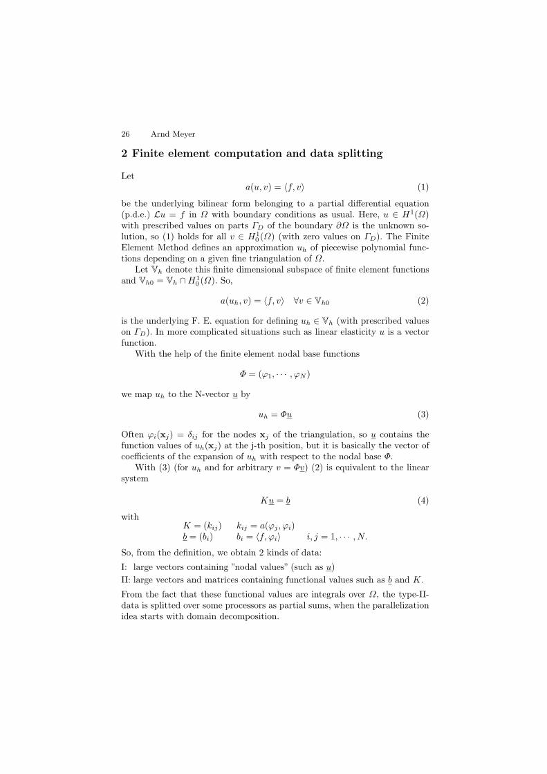
So, from the definition, we obtain 2 kinds of data:
I: large vectors containing ”nodal values” (such as u)
II: large vectors and matrices containing functional values such as b and K.
From the fact that these functional values are integrals over Ω, the type-II-data is splitted over some processors as partial sums, when the parallelizationidea starts with domain decomposition.
Parallel Finite Element Computations 27
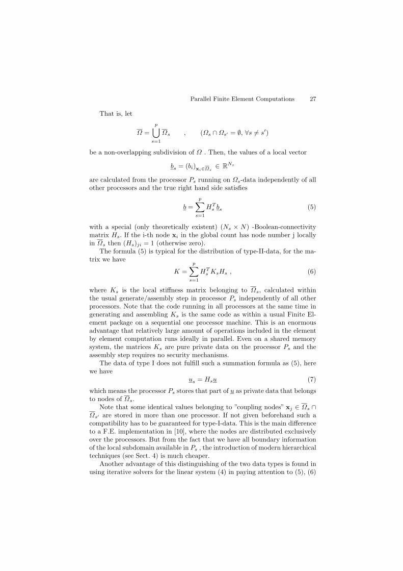
That is, let
Ω =
p⋃
s=1
Ωs , (Ωs ∩Ωs′ = ∅, ∀s = s′)
be a non-overlapping subdivision of Ω . Then, the values of a local vector
bs = (bi)xi∈Ωs∈ R
Ns
are calculated from the processor Ps running on Ωs-data independently of allother processors and the true right hand side satisfies
b =
p∑
s=1
HTs bs (5)
with a special (only theoretically existent) (Ns × N) -Boolean-connectivitymatrix Hs. If the i-th node xi in the global count has node number j locallyin Ωs then (Hs)ji = 1 (otherwise zero).
The formula (5) is typical for the distribution of type-II-data, for the ma-trix we have
K =
p∑
s=1
HTs KsHs , (6)
where Ks is the local stiffness matrix belonging to Ωs, calculated withinthe usual generate/assembly step in processor Ps independently of all otherprocessors. Note that the code running in all processors at the same time ingenerating and assembling Ks is the same code as within a usual Finite El-ement package on a sequential one processor machine. This is an enormousadvantage that relatively large amount of operations included in the elementby element computation runs ideally in parallel. Even on a shared memorysystem, the matrices Ks are pure private data on the processor Ps and theassembly step requires no security mechanisms.
The data of type I does not fulfill such a summation formula as (5), herewe have
us = Hsu (7)
which means the processor Ps stores that part of u as private data that belongsto nodes of Ωs.
Note that some identical values belonging to ”coupling nodes” xj ∈ Ωs ∩Ωs′ are stored in more than one processor. If not given beforehand such acompatibility has to be guaranteed for type-I-data. This is the main differenceto a F.E. implementation in [10], where the nodes are distributed exclusivelyover the processors. But from the fact that we have all boundary informationof the local subdomain available in Ps , the introduction of modern hierarchicaltechniques (see Sect. 4) is much cheaper.
Another advantage of this distinguishing of the two data types is found inusing iterative solvers for the linear system (4) in paying attention to (5), (6)
28 Arnd Meyer
and (7). Here we watch that vectors of same type are updated by vectors ofsame type, so again this requires no data communication over the processors.Moreover, all iterative solvers need at least one matrix–vector–multiply perstep of the iteration. This is nothing else than the calculation of a vector offunctional values, so it changes a type-I into a type-II-vector without any datatransfer again:
Let uh = Φu an arbitrary function in Vh, so u ∈ RN an arbitrary vector,
then v = Ku contains the functional values
vi = a(uh, ϕi) i = 1, · · · , N,
andv =
(∑HT
s KsHs
)u =
∑HT
s Ksus =∑HT
s vs,
whenever vs := Ksus is done locally in processor Ps. From the same reason,the residual vector r = Ku− b of the given linear system is calculated locallyas type-II-data.
3 Data flow within the conjugate gradient method
The preconditioned conjugate gradient method (PCGM) has found to be theappropriate solver for large sparse linear systems, if a good preconditioner canbe introduced. Let this preconditioner signed with C, the modern ideas forconstructing C and the results are given in the next chapters. Then PCGMfor solving Ku = b is the following algorithm.
PCGM
Start: define start vector u
r := Ku− b, q := w := C−1r, γo := γ := rTw
Iteration: until stopping criterion fulfilled do
(1) v := Kq
(2) δ := vT q, α := −γ/δ(3) u := u+ αq
(4) r := r + αv
(5) w := C−1r
(6) γ := rTw, β := γ/γ, γ := γ
(7) q := w + βq
Remark 1: The stopping criterion is often :
γ < γo · tol2 ⇒ stop.

Parallel Finite Element Computations 29
Here, the quantityrTC−1r = zTKC−1Kz
with the actual error z = u− u∗ is decreased by tol2, so the KC−1K−Normof z is decreased by tol.
Remark 2: The convergence is guaranteed if K and C are symmetric, posi-tive definite. The rate of convergence is linear depending on the convergencequotient
η =1−√ξ1 +√ξ
with ξ = λmin(C−1K)/λmax(C−1K).
For the parallel use of this method, we define
u,w, q to be type-I-dataand b, r, v to be type-II-data
(from the above discussions) .
So the steps (1), (3), (4) and (7) do not require any data communication andare pure arithmetical work with private data. The both inner products forδ and γ in step (2) and (6) are simple sums of local inner products over allprocessors:
γ = rTw =(∑
HTs rs
)T
w =∑rTs Hsw =
p∑
s=1
rTs ws.
So the parallel preconditioned conjugate gradient method is the followingalgorithm (running locally in each processor Ps):
PPCGM
Start:Choose u, set us = Hsu in Ps
rs := Ksus − bs, w := C−1r ( with r =∑HT
s rs)set ws = Hsw in Ps
γs := rTs ws γ := γo :=p∑
s=1γs
Iteration: until stopping criterion fulfilled do
30 Arnd Meyer
(1) vs := Ksqs
(2) δs := vTs qs δ :=
p∑s=1δs, α := −γ/δ
(3) us := us + αqs
(4) rs := rs + αvs
(5) w := C−1r (with r =∑HT
s rs)
set ws = Hsw
(6) γs := rTs ws, γ :=p∑
s=1γs, β := γ/γ, γ := γ
(7) qs
:= ws + βqs
Remark 3: The connection between the subdomains Ωs is included instep (5) only, all other steps are pure local calculations or the sum of onenumber over all processors.
A proper definition of the preconditioner C fulfills three requirements:
(A) The arithmetical operations for step (5) are cheap (proportionally tothe number of unknowns)
(B) The condition number κ(C−1K) = ξ−1 is small, independent of thediscretization parameter h (mesh spacing) or only slightly growingfor h→ 0, such as O(|lnh|).
(C) The number of data exchanges between the processors for realizingstep (5) is as small as possible (best: exactly one data exchange ofvalues belonging to the coupling nodes).
Remark 4: For no preconditioning at all ( C = I ) or for the simplediagonal preconditioner ( C = diag(K) ), (A) and (C) are perfectly fulfilled,but (B) not. Here we have κ(C−1K) = O(h−2). So the number of iterationswould grow with h−1 not optimally.
The modern preconditioning techniques such as
• the domain decomposition preconditioner (i.e. local preconditioners forinterior degrees of freedom combined with Schur-complement precondi-tioners on the coupling boundaries, see [1, 3–7])
• hierarchical preconditioners for 2D problems due to Yserentant [9]• Bramble-Pasciak-Xu-preconditioners (and related ones see [1, 8]) for hier-
archical meshes in 2D and 3D
and others have this famous properties. Here (A) and (B) are given fromthe construction and from the analysis. The property (C) is surprisingly ful-filled perfectly. Nearly the same is true, when Multigrid–methods are used aspreconditioner within PPCGM, but from the inherent recursive work on thecoarser meshes, we cannot achieve exactly one data exchange over the cou-pling boundaries per step but L times for an L level grid.
Parallel Finite Element Computations 31
Remark 5: All these modern preconditioners can be found as special casesof the Multiplicative or Additive Schwarz Method (MSM/ASM [8]) dependingon various splittings of the F.E. subspace Vh into special chosen subspaces.
4 An example for a parallel preconditioner
The most simple but efficient example of a preconditioner fulfilling (A), (B),(C) is YSERENTANT’s hierarchical one [9]. Here we have generated the finemesh from L levels subdivision of a given coarse mesh. One level means subdi-viding all triangles into 4 smaller ones of equal size (in the most simple case).Then, additionally to the nodal basis Φ of the fine grid, we can define the socalled hierarchical basis Ψ = (ψ1, · · · , ψN ) spanning the same space V2h. Sothere exists an (N ×N)−matrix Q transforming Φ into Ψ :
Ψ = ΦQ.
From the fact that a stiffness matrix defined with the base Ψ
KH = (a(ψj , ψi))Ni,j=1
would be much better conditioned but nearly dense, we obtain from KH =QTKQ the matrix C = (QQT )−1 as a good preconditioner:
κ(KH) = κ((QQT )K) = κ(C−1K).
From [9] the multiplying w := QQT r can be very cheaply implemented if thelevel by level mesh generation is stored within a special list. Surprisingly, thismultiply is perfectly parallel, if the lists from the mesh subdivision are storedlocally in Ps (mesh in Ωs).
Let w = Qy , y = QT r, then the multiply y = QT r is nothing else thantransforming the functional values of a ”residual functional” ri = 〈r, ϕi〉 withrespect to the nodal base functions into functional values with respect to thehierarchical base functions: yi = 〈r, ψi〉.So this part of the preconditioner transforms type-II-data into type-II-datawithout communication and y =
∑HT
s ys.
Then the type-II-vector y is assembled into type-I
y = y, ys
= ys+∑
j =s
HsHTj yj︸ ︷︷ ︸
from other processors
containing now nodal data, but values belonging to the hierarchical base. Sothe function
w = Φw = Ψy
is represented by w after back transforming
32 Arnd Meyer
w = Qy
This is again a transformation of type-I-data into itself, so the preconditionerrequires exactly one data exchange of values belonging to coupling boundarynodes per step of the PPCGM iteration.
Remark 6: For better convergence, a coarse mesh solver is introduced.Additionally use of Jacobi-preconditioning is a worthy idea for beating jump-ing coefficients and varying mesh spacings etc., so
C−1 = J−1/2Q
(C−1
o OO I
)QTJ−1/2
with J = diag(K).
Remark 7: The better modern BPX-Preconditioners are implementedsimilarly fulfilling (A), (B), (C) in the same way.
5 Examples in linear elasticity
Let us demonstrate the power of this parallel finite element code at a 2Dbenchmark example.
The Dam - Coarse Mesh / Materials
SPC - TU Chemnitz
Fig. 1. Numerical example
We have used the GC Power-Plus-128 parallel computer at TU Chemnitzhaving up to 128 processors PC601 for computation from the years before2000. The maximal arithmetical speed of 80 MFlops/s is never achieved forour typical application with unstructured meshes. Here, the matrix vector
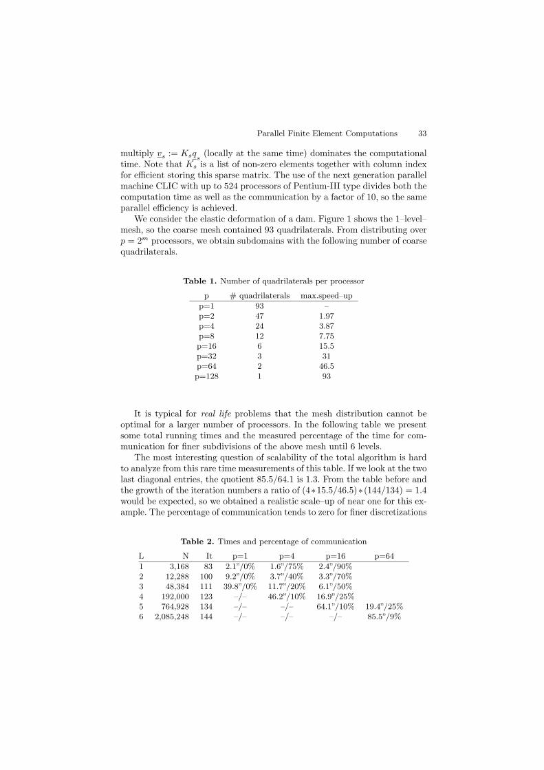
Parallel Finite Element Computations 33
multiply vs := Ksqs (locally at the same time) dominates the computationaltime. Note that Ks is a list of non-zero elements together with column indexfor efficient storing this sparse matrix. The use of the next generation parallelmachine CLIC with up to 524 processors of Pentium-III type divides both thecomputation time as well as the communication by a factor of 10, so the sameparallel efficiency is achieved.
We consider the elastic deformation of a dam. Figure 1 shows the 1–level–mesh, so the coarse mesh contained 93 quadrilaterals. From distributing overp = 2m processors, we obtain subdomains with the following number of coarsequadrilaterals.
Table 1. Number of quadrilaterals per processor
p # quadrilaterals max.speed–up
p=1 93 –p=2 47 1.97p=4 24 3.87p=8 12 7.75p=16 6 15.5p=32 3 31p=64 2 46.5p=128 1 93
It is typical for real life problems that the mesh distribution cannot beoptimal for a larger number of processors. In the following table we presentsome total running times and the measured percentage of the time for com-munication for finer subdivisions of the above mesh until 6 levels.
The most interesting question of scalability of the total algorithm is hardto analyze from this rare time measurements of this table. If we look at the twolast diagonal entries, the quotient 85.5/64.1 is 1.3. From the table before andthe growth of the iteration numbers a ratio of (4∗15.5/46.5)∗(144/134) = 1.4would be expected, so we obtained a realistic scale–up of near one for this ex-ample. The percentage of communication tends to zero for finer discretizations
Table 2. Times and percentage of communication
L N It p=1 p=4 p=16 p=64
1 3,168 83 2.1”/0% 1.6”/75% 2.4”/90%2 12,288 100 9.2”/0% 3.7”/40% 3.3”/70%3 48,384 111 39.8”/0% 11.7”/20% 6.1”/50%4 192,000 123 –/– 46.2”/10% 16.9”/25%5 764,928 134 –/– –/– 64.1”/10% 19.4”/25%6 2,085,248 144 –/– –/– –/– 85.5”/9%
34 Arnd Meyer
and constant number of processors. Much more problematic is the comparisonof two non–equal processor numbers, such as 16 and 64 in the table. Certainly,the larger number of processors requires more communication start–up’s inthe dot–products (log2p). Within the subdomain communication the start-up’s can be equal but need not. This depends on the resulting shapes of thesubdomains within each processor, so the decrease from 10% to 9% in theabove table is typical but very dependent on the example and the distributionprocess.
Whereas such 2D examples give scale–up values of near 90% for fine enoughdiscretizations, much smaller values of the scale–up are achieved in 3D. Thereason is the more complicate connection between the subdomains. Here, wehave the crosspoints, the coupling faces belonging to 2 processors as in 2D butadditionally coupling edges with an unstructured rich relationship betweenthe subdomains. So the data exchange within the preconditioning step (5) ofPPCGM is much more expensive and 50% communication time is typical forour parallel computer.
References
1. J. H. Bramble, J. E. Pasciak, A. H. Schatz (1986-89): The Construction of Pre-conditioners for Elliptic Problems by Substructuring I – IV,Mathematics of Computation, 47:103–134, 1986, 49:1–16, 1987, 51:415–430, 1988,53:1–24, 1989.
2. I. H. Bramble, J. E. Pasciak, J. Xu, Parallel Multilevel Preconditioners, Math.Comp., 55:191, 1-22, 1990.
3. G. Haase, U. Langer, A. Meyer, The Approximate Dirichlet Domain Decomposi-tion Method,Part I: An Algebraic Approach,Part II: Application to 2nd-order Elliptic B.V.P.s,Computing, 47:137-151/153-167, 1991.
4. G. Haase, U. Langer, A. Meyer, Domain Decomposition Preconditioners withInexact Subdomain Solvers,J. Num. Lin. Alg. with Appl., 1:27-42, 1992.
5. G. Haase, U. Langer, A. Meyer, Parallelisierung und Vorkonditionierung des CG-Verfahrens durch Gebietszerlegung,in: G. Bader, et al, eds., Numerische Algorithmen auf Transputer-Systemen, Teub-ner Skripten zur Numerik, B. G. Teubner, Stuttgart 1993.
6. G. Haase, U. Langer, A. Meyer, S.V.Nepommnyaschikh Hierarchical ExtensionOperators and Local Multigrid Methods in Domain Decomposition Precondition-ers, East-West J. Numer. Math., 2:173-193, 1994.
7. A. Meyer, A Parallel Preconditioned Conjugate Gradient Method Using DomainDecomposition and Inexact Solvers on Each Subdomain,Computing, 45:217-234, 1990.
8. P.Oswald, Multilevel Finite Element Approximation: Theory and Applications,Teubner Skripten zur Numerik, B.G.Teubner Stuttgart 1994.
9. H. Yserentant, Two Preconditioners Based on the Multilevel Splitting of FiniteElement Spaces, Numer. Math., 58:163-184, 1990.

Parallel Finite Element Computations 35
10. L.Gross, C.Roll, W.Schonauer, Nonlinear Finite Element Problems on ParallelComputers,In:Dongarra, Wasnievski, eds.,Parallel Scientific Computing, First Int. Workshop PARA ’94, 247-261, 1994.

A Performance Analysis of ABINITon a Cluster System
Torsten Hoefler1, Rebecca Janisch2, and Wolfgang Rehm1
1 Technische Universitat Chemnitz, Fakultat fur Informatik09107 Chemnitz, [email protected] [email protected]
2 Technische Universitat ChemnitzFakultat fur Elektrotechnik und Informationstechnik09107 Chemnitz, [email protected]
1 Introduction
1.1 Electronic structure calculations
In solid state physics, bonding and electronic structure of a material can be in-vestigated by solving the quantum mechanical (time-independent) Schrodingerequation,
HtotΦ = EtotΦ , (1)
in which the Hamilton operator Htot describes all interactions within thesystem. The solution Φ, the wavefunction of the system, describes the stateof all N electrons and M atomic nuclei, and Etot is the total energy of thisstate.Usually, the problem is split by separating the electronic from the ionic part bymaking use of the Born-Oppenheimer approximation [1]. Next we consider theelectrons as independent particles, represented by one-electron wavefunctionsφi. Density functional theory (DFT), based on the work of Hohenberg andKohn [2] and Kohn and Sham [3], then enables us to represent the totalelectronic energy of the system by a functional of the electron density n(r):
n(r) =∑
i
|φi|2 (2)
→ E = E [n(r)] = F [n] +
∫Vext(r)n(r)dr
= Ekin[n] + EH[n] + Exc[n] +
∫Vext(r)n(r)dr . (3)
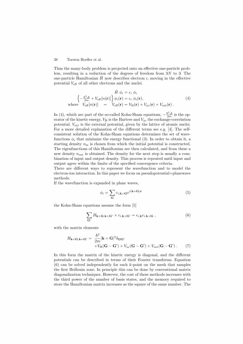
38 Torsten Hoefler et al.
Thus the many-body problem is projected onto an effective one-particle prob-lem, resulting in a reduction of the degrees of freedom from 3N to 3. Theone-particle Hamiltonian H now describes electron i, moving in the effectivepotential Veff of all other electrons and the nuclei.
H φi = ǫi φi−
2∆2m + Veff [n(r)]
φi(r) = ǫi φi(r),
where Veff [n(r)] = Veff(r) = VH(r) + Vxc(r) + Vext(r) .
(4)
In (4), which are part of the so-called Kohn-Sham equations, −2∆2m is the op-
erator of the kinetic energy, VH is the Hartree and Vxc the exchange-correlationpotential. Vext is the external potential, given by the lattice of atomic nuclei.For a more detailed explanation of the different terms see e.g. [4]. The self-consistent solution of the Kohn-Sham equations determines the set of wave-functions φi that minimize the energy functional (3). In order to obtain it, astarting density nin is chosen from which the initial potential is constructed.The eigenfunctions of this Hamiltonian are then calculated, and from these anew density nout is obtained. The density for the next step is usually a com-bination of input and output density. This process is repeated until input andoutput agree within the limits of the specified convergence criteria.There are different ways to represent the wavefunction and to model theelectron-ion interaction. In this paper we focus on pseudopotential+planewavemethods.If the wavefunction is expanded in plane waves,
φi =∑
G
ci,k+Gei(k+G)r (5)
the Kohn-Sham equations assume the form [5]
∑
G′
Hk+G,k+G′ × ci,k+G′ = ǫi,kci,k+G , (6)
with the matrix elements
Hk+G,k+G′ =
2
2m|k + G|2δGG′
+VH(G−G′) + Vxc(G−G′) + Vext(G−G′) . (7)
In this form the matrix of the kinetic energy is diagonal, and the differentpotentials can be described in terms of their Fourier transforms. Equation(6) can be solved independently for each k-point on the mesh that samplesthe first Brillouin zone. In principle this can be done by conventional matrixdiagonalization techniques. However, the cost of these methods increases withthe third power of the number of basis states, and the memory required tostore the Hamiltonian matrix increases as the square of the same number. The

A Performance Analysis of ABINIT on a Cluster System 39
number of plane waves in the basis is determined by the choice of the cutoffenergy Ecut =
2/2m|k+Gcut|2 and is typically of the order of 100 per atom, ifnorm-conserving pseudopotentials are used. Therefore alternative techniqueshave been developed to minimize the Kohn-Sham energy functional (3), e.g.by conjugate gradient (CG) methods (for an introduction to this method seee.g. [6]). In a band-by-band CG scheme one eigenvalue (band) ǫi,k is obtainedat a time, and the corresponding eigenvector is orthogonalized with respectto the previously obtained ones.
1.2 The ABINIT code
ABINIT [7] is an open source code for ab initio electronic structure calcu-lations based on the DFT described in Sect. 1.1. The code is the object ofan ongoing open software project of the Universite Catholique de Louvain,Corning Incorporated, and other contributors [8] .
ABINIT mostly aims at solid state research, in the sense that periodicboundary conditions are applied and the majority of the integrals that haveto be calculated are represented in reciprocal space (k-space). It currently fea-tures the calculation of various electronic ground state properties (total en-ergy, bandstructure, density of states,..), and several structural optimizationroutines. Furthermore it enables the investigation of electric and magnetic po-larization and electronic excitations. Originally a pseudopotential+planewavecode, ABINIT for a short time (since version 4.2.x) also features the projector-augmented wave method, but this is still under developement. In the followingwe refer to the planewave method.To begin the self-consistency cycle, a starting density is constructed, and astarting potential derived. The eigenvalues and eigenvectors are determined bya band-by-band CG scheme [5], during which the density (i.e. the potential) iskept fixed until the whole set of functions has been obtained. The alternativeof updating the density with each new band has been abandoned, to makea simple parallelization of the calculation over the k-points possible. Only atthe end of one CG loop is the density updated by the scheme of choice (e.g.simple mixing, or Anderson mixing). For a comparison of different schemes seee.g. [9]). A more detailed description of the DFT implementation in generalis given in [10].
Different levels of parallelization are implemented. The most efficient par-allelization is the distribution of the k-points that are used to sample theBrillouin zone on different processors. Unfortunately the necessary number ofk-points decreases with increasing system size, so the scaling with the num-ber of atoms is rather unfavourable. One can partially make up for this bydistributing the work related to different states (or bands) within a given k-point. Since the number of states increases with the system size, the overall
40 Torsten Hoefler et al.
scaling with number of atoms improves. For example a blocked conjugate gra-dient algorithm can be used to optimize the wavefunctions, which provides thepossibility to parallelize over the states within one block. Instead of a singleeigenstate, as in the band-by-band scheme, nbdblock states are determinedat the same time, where nbdblock is the number of bands in one block. Ofcourse this leads to a small increase in the time that is needed to orthogonalizethe eigenvectors with respect to those obtained previously. Furthermore, toguarantee convergence, a too high value for nbdblock should not be chosen.The ABINIT manual advises nbdblock ≤ 4 as a meaningful choice.Both methods, k-point parallelization and parallelization over bands, are im-plemented using the MPI library. A third possibility of parallelization is givenby the distribution of the work related to different wavefunction coefficients,which is realized with OpenMP compiler directives. It is used for example inthe parallelization of the FFT algorithm, but this feature is still under devel-opement.
These parallelization methods, which are based on the underlying physicsof the calculation, are useful only for a finite number of CPUs (a fact, thatis not a special property of ABINIT, but common to all electronic structurecodes). In a practical calculation, the required number of k-points, nkpt, for aspecific geometry is determined by convergence tests. To decrease the compu-tational effort, the k-point parallelization is then the first method of choice.The best speedup is achieved if the number of k-points is an integer multipleof the number of CPUs:
nkpt = n×NCPU with n ∈ N. (8)
Ideally, n = 1.If the number of available CPUs is larger than the number of k-points neededfor the calculation, the speedup saturates. In this case, the additional paral-lelization over bands can improve the performance of ABINIT, if
NCPU = nbdblock× nkpt . (9)
In principle the parallelization scheme also works forNCPU = nbdblock, whichresults in a parallelization over bands only. However, this is rather inefficient,as will be seen below.
1.3 Related work
The biggest challenge after programming a parallel application is to optimizeit according to a given parallel architecture. The first step of each optimizationprocess is the performance and scalability measurement which is often calledbenchmarking. There are methods based on theoretical simulation [11,12] andmethods based on benchmarking [13, 14]. There are also studies which try to
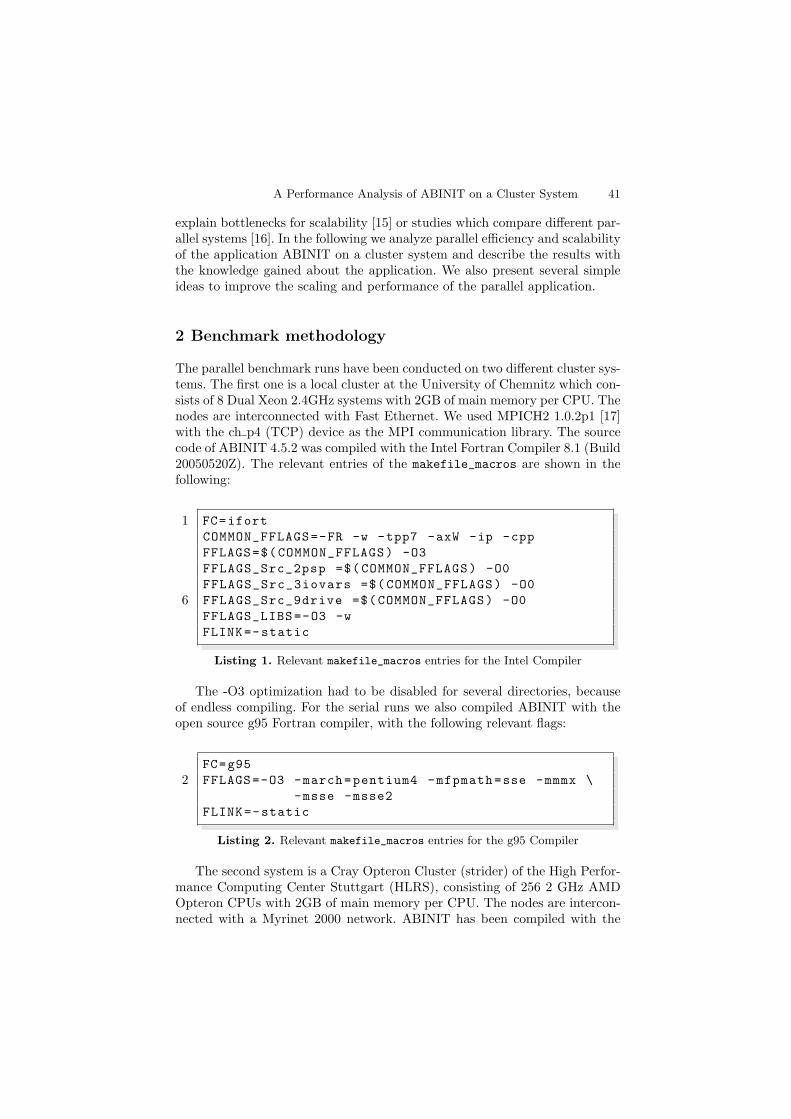
A Performance Analysis of ABINIT on a Cluster System 41
explain bottlenecks for scalability [15] or studies which compare different par-allel systems [16]. In the following we analyze parallel efficiency and scalabilityof the application ABINIT on a cluster system and describe the results withthe knowledge gained about the application. We also present several simpleideas to improve the scaling and performance of the parallel application.
2 Benchmark methodology
The parallel benchmark runs have been conducted on two different cluster sys-tems. The first one is a local cluster at the University of Chemnitz which con-sists of 8 Dual Xeon 2.4GHz systems with 2GB of main memory per CPU. Thenodes are interconnected with Fast Ethernet. We used MPICH2 1.0.2p1 [17]with the ch p4 (TCP) device as the MPI communication library. The sourcecode of ABINIT 4.5.2 was compiled with the Intel Fortran Compiler 8.1 (Build20050520Z). The relevant entries of the makefile_macros are shown in thefollowing:
1 FC=ifort
COMMON_FFLAGS=-FR -w -tpp7 -axW -ip -cpp
FFLAGS=$(COMMON_FFLAGS) -O3
FFLAGS_Src_2psp =$(COMMON_FFLAGS) -O0
FFLAGS_Src_3iovars =$(COMMON_FFLAGS) -O0
6 FFLAGS_Src_9drive =$(COMMON_FFLAGS) -O0
FFLAGS_LIBS=-O3 -w
FLINK=-static
Listing 1. Relevant makefile_macros entries for the Intel Compiler
The -O3 optimization had to be disabled for several directories, becauseof endless compiling. For the serial runs we also compiled ABINIT with theopen source g95 Fortran compiler, with the following relevant flags:
FC=g95
2 FFLAGS=-O3 -march=pentium4 -mfpmath=sse -mmmx \
-msse -msse2
FLINK=-static
Listing 2. Relevant makefile_macros entries for the g95 Compiler
The second system is a Cray Opteron Cluster (strider) of the High Perfor-mance Computing Center Stuttgart (HLRS), consisting of 256 2 GHz AMDOpteron CPUs with 2GB of main memory per CPU. The nodes are intercon-nected with a Myrinet 2000 network. ABINIT has been compiled with the
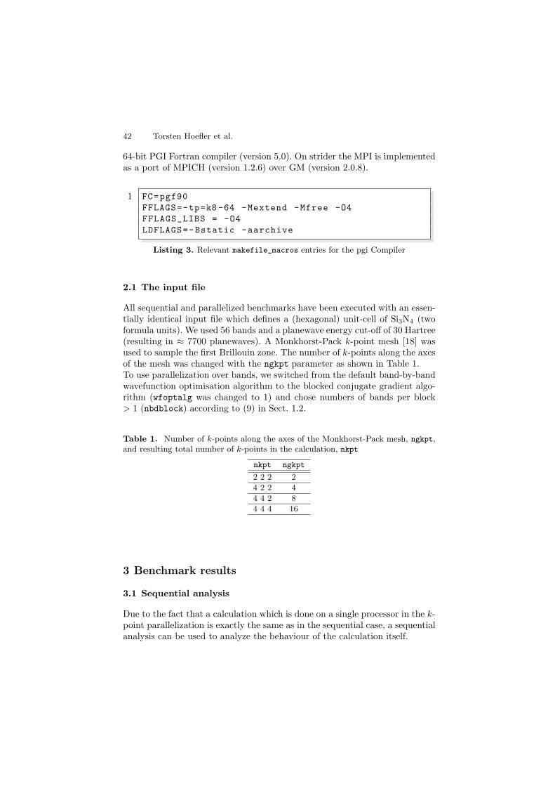
42 Torsten Hoefler et al.
64-bit PGI Fortran compiler (version 5.0). On strider the MPI is implementedas a port of MPICH (version 1.2.6) over GM (version 2.0.8).
1 FC=pgf90
FFLAGS=-tp=k8 -64 -Mextend -Mfree -O4
FFLAGS_LIBS = -O4
LDFLAGS=-Bstatic -aarchive
Listing 3. Relevant makefile_macros entries for the pgi Compiler
2.1 The input file
All sequential and parallelized benchmarks have been executed with an essen-tially identical input file which defines a (hexagonal) unit-cell of Si3N4 (twoformula units). We used 56 bands and a planewave energy cut-off of 30 Hartree(resulting in ≈ 7700 planewaves). A Monkhorst-Pack k-point mesh [18] wasused to sample the first Brillouin zone. The number of k-points along the axesof the mesh was changed with the ngkpt parameter as shown in Table 1.To use parallelization over bands, we switched from the default band-by-bandwavefunction optimisation algorithm to the blocked conjugate gradient algo-rithm (wfoptalg was changed to 1) and chose numbers of bands per block> 1 (nbdblock) according to (9) in Sect. 1.2.
Table 1. Number of k-points along the axes of the Monkhorst-Pack mesh, ngkpt,and resulting total number of k-points in the calculation, nkpt
nkpt ngkpt
2 2 2 2
4 2 2 4
4 4 2 8
4 4 4 16
3 Benchmark results
3.1 Sequential analysis
Due to the fact that a calculation which is done on a single processor in the k-point parallelization is exactly the same as in the sequential case, a sequentialanalysis can be used to analyze the behaviour of the calculation itself.
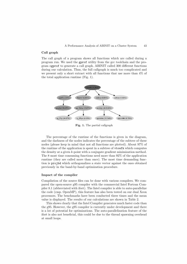
A Performance Analysis of ABINIT on a Cluster System 43
Call graph
The call graph of a program shows all functions which are called during aprogram run. We used the gprof utility from the gcc toolchain and the pro-gram cgprof to generate a call graph. ABINIT called 300 different functionsduring our calculation. Thus, the full callgraph is much too complicated andwe present only a short extract with all functions that use more than 4% ofthe total application runtime (Fig. 1).
Fig. 1. The partial callgraph
The percentage of the runtime of the functions is given in the diagram,and the darkness of the nodes indicates the percentage of the subtree of thesenodes (please keep in mind that not all functions are plotted). About 97% ofthe runtime of the application is spent in a subtree of vtowfk which computesthe density at a given k-point with a conjugate gradient minimization method.The 8 most time consuming functions need more than 92% of the applicationruntime (they are called more than once). The most time demanding func-tion is projbd which orthogonalizes a state vector against the ones obtainedpreviously in the band-by-band optimization procedure.
Impact of the compiler
Compilation of the source files can be done with various compilers. We com-pared the open-source g95 compiler with the commercial Intel Fortran Com-piler 8.1 (abbreviated with ifort). The Intel compiler is able to auto-parallelizethe code (cmp. OpenMP), this feature has also been tested on our dual Xeonprocessors. The benchmarks have been conducted three times and the meanvalue is displayed. The results of our calculations are shown in Table 2.
This shows clearly that the Intel Compiler generates much faster code thanthe g95. However, the g95 compiler is currently under development and thereis a lot of potential for optimizations. The auto-parallelization feature of theifort is also not beneficial, this could be due to the thread spawning overheadat small loops.
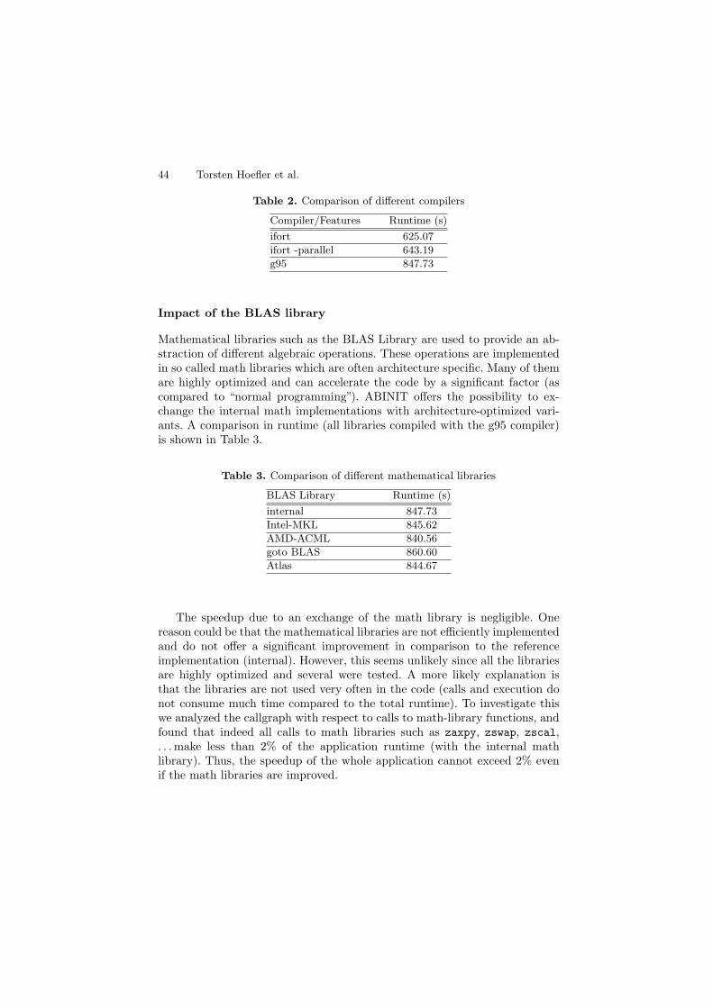
44 Torsten Hoefler et al.
Table 2. Comparison of different compilers
Compiler/Features Runtime (s)
ifort 625.07
ifort -parallel 643.19
g95 847.73
Impact of the BLAS library
Mathematical libraries such as the BLAS Library are used to provide an ab-straction of different algebraic operations. These operations are implementedin so called math libraries which are often architecture specific. Many of themare highly optimized and can accelerate the code by a significant factor (ascompared to “normal programming”). ABINIT offers the possibility to ex-change the internal math implementations with architecture-optimized vari-ants. A comparison in runtime (all libraries compiled with the g95 compiler)is shown in Table 3.
Table 3. Comparison of different mathematical libraries
BLAS Library Runtime (s)
internal 847.73
Intel-MKL 845.62
AMD-ACML 840.56
goto BLAS 860.60
Atlas 844.67
The speedup due to an exchange of the math library is negligible. Onereason could be that the mathematical libraries are not efficiently implementedand do not offer a significant improvement in comparison to the referenceimplementation (internal). However, this seems unlikely since all the librariesare highly optimized and several were tested. A more likely explanation isthat the libraries are not used very often in the code (calls and execution donot consume much time compared to the total runtime). To investigate thiswe analyzed the callgraph with respect to calls to math-library functions, andfound that indeed all calls to math libraries such as zaxpy, zswap, zscal,. . . make less than 2% of the application runtime (with the internal mathlibrary). Thus, the speedup of the whole application cannot exceed 2% evenif the math libraries are improved.
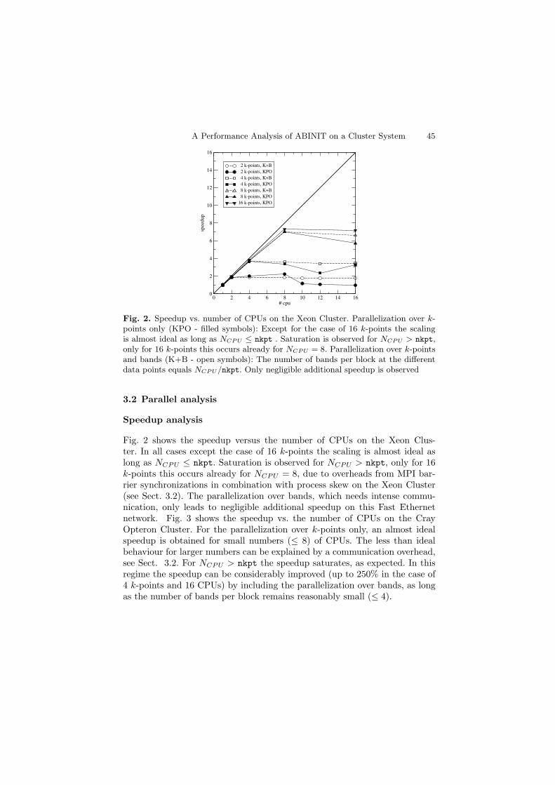
A Performance Analysis of ABINIT on a Cluster System 45
0 2 4 6 8 10 12 14 16# cpu
0
2
4
6
8
10
12
14
16
spee
dup
2 k-points, K+B
2 k-points, KPO
4 k-points, K+B
4 k-points, KPO
8 k-points, K+B
8 k-points, KPO
16 k-points, KPO
Fig. 2. Speedup vs. number of CPUs on the Xeon Cluster. Parallelization over k-points only (KPO - filled symbols): Except for the case of 16 k-points the scalingis almost ideal as long as NCPU ≤ nkpt . Saturation is observed for NCPU > nkpt,only for 16 k-points this occurs already for NCPU = 8. Parallelization over k-pointsand bands (K+B - open symbols): The number of bands per block at the differentdata points equals NCPU/nkpt. Only negligible additional speedup is observed
3.2 Parallel analysis
Speedup analysis
Fig. 2 shows the speedup versus the number of CPUs on the Xeon Clus-ter. In all cases except the case of 16 k-points the scaling is almost ideal aslong as NCPU ≤ nkpt. Saturation is observed for NCPU > nkpt, only for 16k-points this occurs already for NCPU = 8, due to overheads from MPI bar-rier synchronizations in combination with process skew on the Xeon Cluster(see Sect. 3.2). The parallelization over bands, which needs intense commu-nication, only leads to negligible additional speedup on this Fast Ethernetnetwork. Fig. 3 shows the speedup vs. the number of CPUs on the CrayOpteron Cluster. For the parallelization over k-points only, an almost idealspeedup is obtained for small numbers (≤ 8) of CPUs. The less than idealbehaviour for larger numbers can be explained by a communication overhead,see Sect. 3.2. For NCPU > nkpt the speedup saturates, as expected. In thisregime the speedup can be considerably improved (up to 250% in the case of4 k-points and 16 CPUs) by including the parallelization over bands, as longas the number of bands per block remains reasonably small (≤ 4).
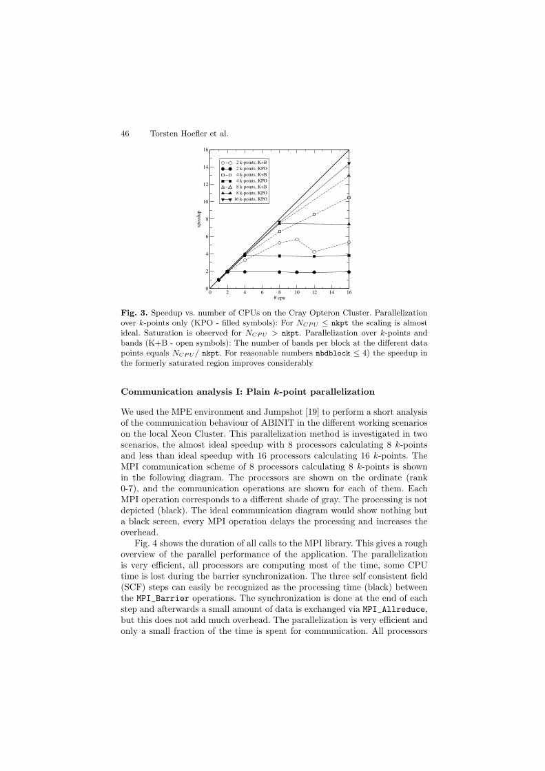
46 Torsten Hoefler et al.
0 2 4 6 8 10 12 14 16# cpu
0
2
4
6
8
10
12
14
16
spee
dup
2 k-points, K+B
2 k-points, KPO
4 k-points, K+B
4 k-points, KPO
8 k-points, K+B
8 k-points, KPO
16 k-points, KPO
Fig. 3. Speedup vs. number of CPUs on the Cray Opteron Cluster. Parallelizationover k-points only (KPO - filled symbols): For NCPU ≤ nkpt the scaling is almostideal. Saturation is observed for NCPU > nkpt. Parallelization over k-points andbands (K+B - open symbols): The number of bands per block at the different datapoints equals NCPU/ nkpt. For reasonable numbers nbdblock ≤ 4) the speedup inthe formerly saturated region improves considerably
Communication analysis I: Plain k-point parallelization
We used the MPE environment and Jumpshot [19] to perform a short analysisof the communication behaviour of ABINIT in the different working scenarioson the local Xeon Cluster. This parallelization method is investigated in twoscenarios, the almost ideal speedup with 8 processors calculating 8 k-pointsand less than ideal speedup with 16 processors calculating 16 k-points. TheMPI communication scheme of 8 processors calculating 8 k-points is shownin the following diagram. The processors are shown on the ordinate (rank0-7), and the communication operations are shown for each of them. EachMPI operation corresponds to a different shade of gray. The processing is notdepicted (black). The ideal communication diagram would show nothing buta black screen, every MPI operation delays the processing and increases theoverhead.
Fig. 4 shows the duration of all calls to the MPI library. This gives a roughoverview of the parallel performance of the application. The parallelizationis very efficient, all processors are computing most of the time, some CPUtime is lost during the barrier synchronization. The three self consistent field(SCF) steps can easily be recognized as the processing time (black) betweenthe MPI_Barrier operations. The synchronization is done at the end of eachstep and afterwards a small amount of data is exchanged via MPI_Allreduce,but this does not add much overhead. The parallelization is very efficient andonly a small fraction of the time is spent for communication. All processors
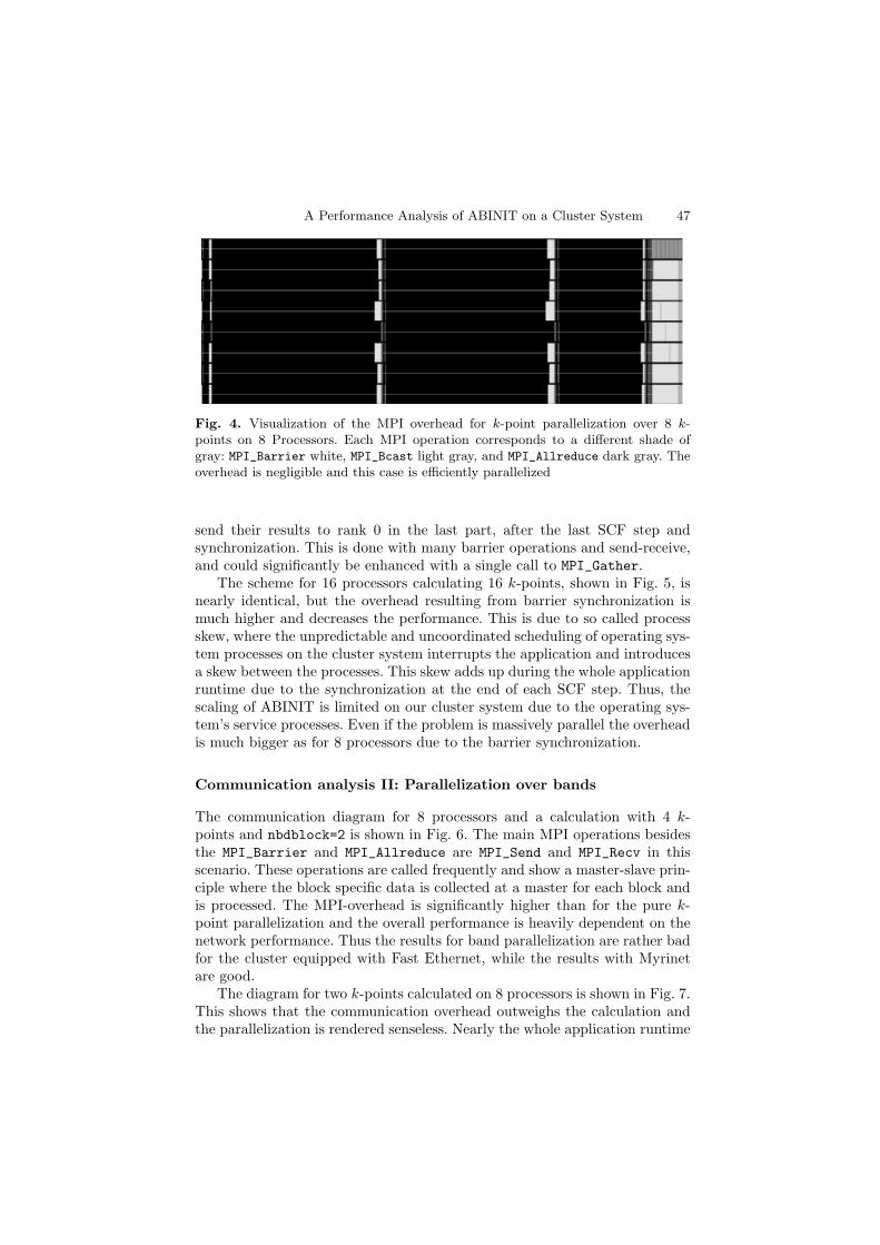
A Performance Analysis of ABINIT on a Cluster System 47
Fig. 4. Visualization of the MPI overhead for k-point parallelization over 8 k-points on 8 Processors. Each MPI operation corresponds to a different shade ofgray: MPI_Barrier white, MPI_Bcast light gray, and MPI_Allreduce dark gray. Theoverhead is negligible and this case is efficiently parallelized
send their results to rank 0 in the last part, after the last SCF step andsynchronization. This is done with many barrier operations and send-receive,and could significantly be enhanced with a single call to MPI_Gather.
The scheme for 16 processors calculating 16 k-points, shown in Fig. 5, isnearly identical, but the overhead resulting from barrier synchronization ismuch higher and decreases the performance. This is due to so called processskew, where the unpredictable and uncoordinated scheduling of operating sys-tem processes on the cluster system interrupts the application and introducesa skew between the processes. This skew adds up during the whole applicationruntime due to the synchronization at the end of each SCF step. Thus, thescaling of ABINIT is limited on our cluster system due to the operating sys-tem’s service processes. Even if the problem is massively parallel the overheadis much bigger as for 8 processors due to the barrier synchronization.
Communication analysis II: Parallelization over bands
The communication diagram for 8 processors and a calculation with 4 k-points and nbdblock=2 is shown in Fig. 6. The main MPI operations besidesthe MPI_Barrier and MPI_Allreduce are MPI_Send and MPI_Recv in thisscenario. These operations are called frequently and show a master-slave prin-ciple where the block specific data is collected at a master for each block andis processed. The MPI-overhead is significantly higher than for the pure k-point parallelization and the overall performance is heavily dependent on thenetwork performance. Thus the results for band parallelization are rather badfor the cluster equipped with Fast Ethernet, while the results with Myrinetare good.
The diagram for two k-points calculated on 8 processors is shown in Fig. 7.This shows that the communication overhead outweighs the calculation andthe parallelization is rendered senseless. Nearly the whole application runtime
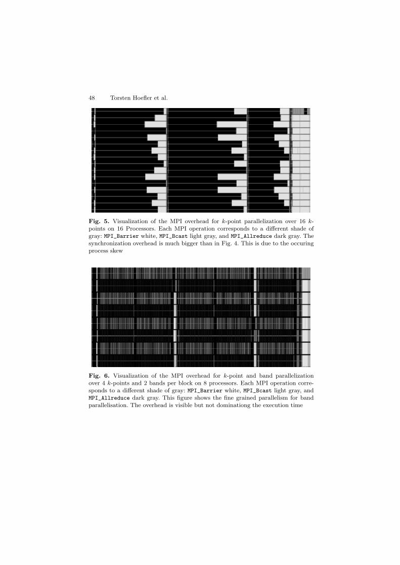
48 Torsten Hoefler et al.
Fig. 5. Visualization of the MPI overhead for k-point parallelization over 16 k-points on 16 Processors. Each MPI operation corresponds to a different shade ofgray: MPI_Barrier white, MPI_Bcast light gray, and MPI_Allreduce dark gray. Thesynchronization overhead is much bigger than in Fig. 4. This is due to the occuringprocess skew
Fig. 6. Visualization of the MPI overhead for k-point and band parallelizationover 4 k-points and 2 bands per block on 8 processors. Each MPI operation corre-sponds to a different shade of gray: MPI_Barrier white, MPI_Bcast light gray, andMPI_Allreduce dark gray. This figure shows the fine grained parallelism for bandparallelisation. The overhead is visible but not dominationg the execution time
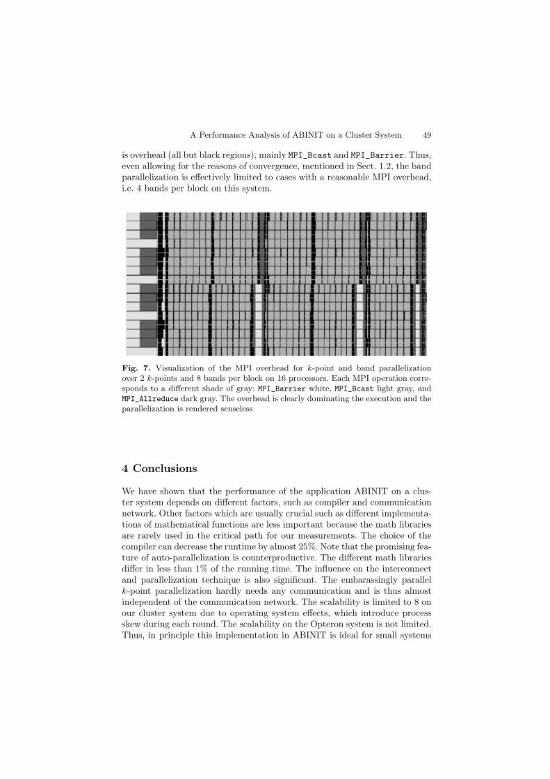
A Performance Analysis of ABINIT on a Cluster System 49
is overhead (all but black regions), mainly MPI_Bcast and MPI_Barrier. Thus,even allowing for the reasons of convergence, mentioned in Sect. 1.2, the bandparallelization is effectively limited to cases with a reasonable MPI overhead,i.e. 4 bands per block on this system.
Fig. 7. Visualization of the MPI overhead for k-point and band parallelizationover 2 k-points and 8 bands per block on 16 processors. Each MPI operation corre-sponds to a different shade of gray: MPI_Barrier white, MPI_Bcast light gray, andMPI_Allreduce dark gray. The overhead is clearly dominating the execution and theparallelization is rendered senseless
4 Conclusions
We have shown that the performance of the application ABINIT on a clus-ter system depends on different factors, such as compiler and communicationnetwork. Other factors which are usually crucial such as different implementa-tions of mathematical functions are less important because the math librariesare rarely used in the critical path for our measurements. The choice of thecompiler can decrease the runtime by almost 25%. Note that the promising fea-ture of auto-parallelization is counterproductive. The different math librariesdiffer in less than 1% of the running time. The influence on the interconnectand parallelization technique is also significant. The embarassingly parallelk-point parallelization hardly needs any communication and is thus almostindependent of the communication network. The scalability is limited to 8 onour cluster system due to operating system effects, which introduce processskew during each round. The scalability on the Opteron system is not limited.Thus, in principle this implementation in ABINIT is ideal for small systems

50 Torsten Hoefler et al.
demanding a lot of k-points, e.g. metals. For systems demanding large super-cells, the communication wise more demanding band parallelization becomesattractive. However, the use of this implementation is only advantageous if afast interconnect can be used for communication. Fast Ethernet is not suitablefor this task.
Acknowledgements
The authors would like to thank X. Gonze for helpful comments. R.J. ac-knowledges the HLRS for a free trial account on the Cray Opteron Clusterstrider.
References
1. M. Born and J.R. Oppenheimer. Zur Quantentheorie der Molekeln. Ann. Physik,84:457, 1927.
2. P. Hohenberg and W. Kohn. Inhomogeneous electron gas. Phys. Rev., 136:B864,1964.
3. W. Kohn and L.J. Sham. Self-consistent equations including exchange andcorrelation effects. Phys. Rev, 140:A1133, 1965.
4. R. M. Martin. Electronic Structure. Cambridge University Press, Cambridge,UK, 2004.
5. M.C. Payne, M.P. Teter, D.C. Allan, T.A. Arias, and J.D. Joannopoulos. Itera-tive minimization techniques for ab initio total-energy calculations - moleculardynamics and conjugate gradients. Rev. Mod. Phys., 64:1045, 1992.
6. J. Nocedal. Theory of algorithms for unconstrained optimization. Acta Num.,page 199, 1991.
7. X. Gonze, G.-M. Rignanese, M. Verstraete, J.-M. Beuken, Y. Pouillon, R. Cara-cas, F. Jollet, M. Torrent, G. Zerah, M. Mikami, P. Ghosez, M. Veithen, J.-Y.Raty, V. Olevano, F. Bruneval, L. Reining, R. Godby, G. Onida, D.R. Hamann,and D.C. Allan. A brief introduction to the ABINIT software package. Z.Kristallogr., 220:558, 2005.
8. http://www.abinit.org/.9. V. Eyert. A comparative study on methods for convergence acceleration of
iterative vector sequences. J.Comp.Phys., 124:271, 1995.10. X. Gonze, J.-M. Beuken, R. Caracas, F. Detraux, M. Fuchs, G.-M. Rignanese,
L. Sindic, M. Verstraete, G. Zerah, F. Jollet, M. Torrent, A. Roy, M. Mikami, Ph.Ghosez, J.-Y. Raty, and D.C. Allan. First-principles computation of materialproperties: the ABINIT software project. Comp. Mat. Sci., 25:478, 2002.
11. A.D. Malony, V. Mertsiotakis, and A. Quick. Automatic scalability analysis ofparallel programs based on modeling techniques. In Proceedings of the 7th inter-national conference on Computer performance evaluation : modelling techniquesand tools, pages 139–158, Secaucus, NJ, USA, 1994. Springer-Verlag New York,Inc.
12. R.J. Block, S. Sarukkai, and P. Mehra. Automated performance predictionof message-passing parallel programs. In Proceedings of the 1995 ACM/IEEEconference on Supercomputing, 1995.
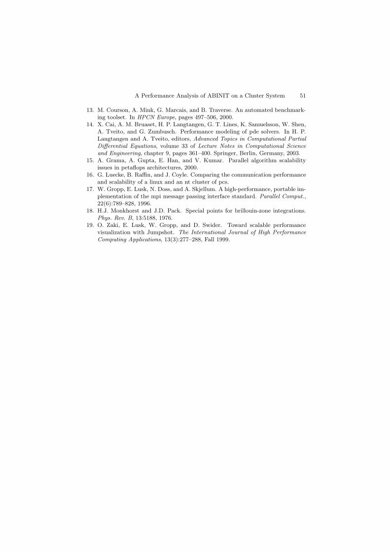
A Performance Analysis of ABINIT on a Cluster System 51
13. M. Courson, A. Mink, G. Marcais, and B. Traverse. An automated benchmark-ing toolset. In HPCN Europe, pages 497–506, 2000.
14. X. Cai, A. M. Bruaset, H. P. Langtangen, G. T. Lines, K. Samuelsson, W. Shen,A. Tveito, and G. Zumbusch. Performance modeling of pde solvers. In H. P.Langtangen and A. Tveito, editors, Advanced Topics in Computational PartialDifferential Equations, volume 33 of Lecture Notes in Computational Scienceand Engineering, chapter 9, pages 361–400. Springer, Berlin, Germany, 2003.
15. A. Grama, A. Gupta, E. Han, and V. Kumar. Parallel algorithm scalabilityissues in petaflops architectures, 2000.
16. G. Luecke, B. Raffin, and J. Coyle. Comparing the communication performanceand scalability of a linux and an nt cluster of pcs.
17. W. Gropp, E. Lusk, N. Doss, and A. Skjellum. A high-performance, portable im-plementation of the mpi message passing interface standard. Parallel Comput.,22(6):789–828, 1996.
18. H.J. Monkhorst and J.D. Pack. Special points for brillouin-zone integrations.Phys. Rev. B, 13:5188, 1976.
19. O. Zaki, E. Lusk, W. Gropp, and D. Swider. Toward scalable performancevisualization with Jumpshot. The International Journal of High PerformanceComputing Applications, 13(3):277–288, Fall 1999.

Some Aspects of Parallel Postprocessingfor Numerical Simulation
Matthias Pester
Technische Universitat Chemnitz, Fakultat fur Mathematik09107 Chemnitz, [email protected]
1 Introduction
The topics discussed in this paper are closely connected to the development ofparallel finite element algorithms and software based on domain decomposition[1, 2]. Numerical simulation on parallel computers generally produces data inlarge quantities being kept in the distributed memory. Traditional methods ofpostprocessing by storing all data and processing the files with other specialsoftware in order to obtain nice pictures may easily fail due to the amount ofmemory and time required.
On the other hand, developing new and efficient parallel algorithms in-volves the necessity to evaluate the behavior of an algorithm immediatelyas an on-line response. Thus, we had to develop a set of visualization toolsfor parallel numerical simulation which is rather quick than perfect, but stillexpressive. The numerical data can be completely processed in parallel andonly the resulting image is displayed on the user’s desktop computer while thenumerical simulation is still running on the parallel machine.
This software package for parallel postprocessing is supplemented by inter-faces to external software running on high-performance graphic workstations,either storing files for an off-line postprocessing or using a TCP/IP streamconnection for on-line data exchange.
2 Pre- and postprocessing interfacesin parallel computation
The main purpose of parallel computers in the field of numerical simulationis number crunching. The discretization of mathematical equations and therefinement of the meshes within the domain of interest lead to large arraysof numerical data which are stored in the distributed memory of a MIMDcomputer. The tasks of pre- and postprocessing, however, are not the primary
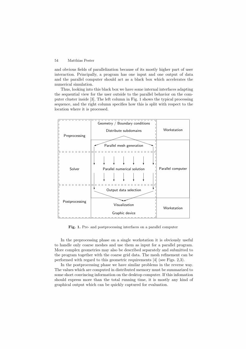
54 Matthias Pester
and obvious fields of parallelization because of its mostly higher part of userinteraction. Principally, a program has one input and one output of dataand the parallel computer should act as a black box which accelerates thenumerical simulation.
Thus, looking into this black box we have some internal interfaces adaptingthe sequential view for the user outside to the parallel behavior on the com-puter cluster inside [3]. The left column in Fig. 1 shows the typical processingsequence, and the right column specifies how this is split with respect to thelocation where it is processed.
Preprocessing
Solver
Postprocessing
Geometry / Boundary conditions
Parallel numerical solution
Graphic device
Distribute subdomains
Parallel mesh generation
Output data selection
Visualization
Parallel computer
Workstation
Workstation
Fig. 1. Pre- and postprocessing interfaces on a parallel computer
In the preprocessing phase on a single workstation it is obviously usefulto handle only coarse meshes and use them as input for a parallel program.More complex geometries may also be described separately and submitted tothe program together with the coarse grid data. The mesh refinement can beperformed with regard to this geometric requirements [4] (see Figs. 2,3).
In the postprocessing phase we have similar problems in the reverse way.The values which are computed in distributed memory must be summarized tosome short convincing information on the desktop computer. If this infomationshould express more than the total running time, it is mostly any kind ofgraphical output which can be quickly captured for evaluation.
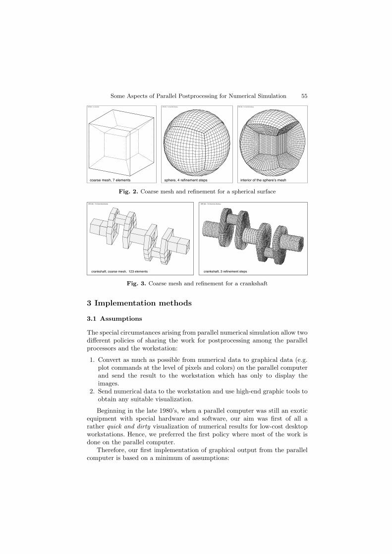
Some Aspects of Parallel Postprocessing for Numerical Simulation 55
coarse mesh, 7 elements
SFB 393 - TU Chemnitz
sphere, 4 refinement steps
SFB 393 - TU Chemnitz-Zwickau
interior of the sphere’s mesh
SFB 393 - TU Chemnitz-Zwickau
Fig. 2. Coarse mesh and refinement for a spherical surface
crankshaft, coarse mesh, 123 elements
SFB 393 - TU Chemnitz-Zwickau
crankshaft, 3 refinement steps
SFB 393 - TU Chemnitz-Zwickau
Fig. 3. Coarse mesh and refinement for a crankshaft
3 Implementation methods
3.1 Assumptions
The special circumstances arising from parallel numerical simulation allow twodifferent policies of sharing the work for postprocessing among the parallelprocessors and the workstation:
1. Convert as much as possible from numerical data to graphical data (e.g.plot commands at the level of pixels and colors) on the parallel computerand send the result to the workstation which has only to display theimages.
2. Send numerical data to the workstation and use high-end graphic tools toobtain any suitable visualization.
Beginning in the late 1980’s, when a parallel computer was still an exoticequipment with special hardware and software, our aim was first of all arather quick and dirty visualization of numerical results for low-cost desktopworkstations. Hence, we preferred the first policy where most of the work isdone on the parallel computer.
Therefore, our first implementation of graphical output from the parallelcomputer is based on a minimum of assumptions:
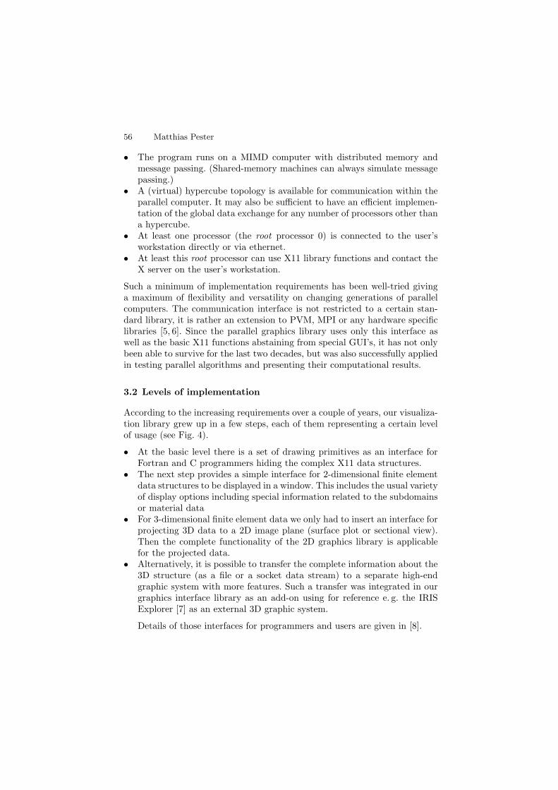
56 Matthias Pester
• The program runs on a MIMD computer with distributed memory andmessage passing. (Shared-memory machines can always simulate messagepassing.)
• A (virtual) hypercube topology is available for communication within theparallel computer. It may also be sufficient to have an efficient implemen-tation of the global data exchange for any number of processors other thana hypercube.
• At least one processor (the root processor 0) is connected to the user’sworkstation directly or via ethernet.
• At least this root processor can use X11 library functions and contact theX server on the user’s workstation.
Such a minimum of implementation requirements has been well-tried givinga maximum of flexibility and versatility on changing generations of parallelcomputers. The communication interface is not restricted to a certain stan-dard library, it is rather an extension to PVM, MPI or any hardware specificlibraries [5, 6]. Since the parallel graphics library uses only this interface aswell as the basic X11 functions abstaining from special GUI’s, it has not onlybeen able to survive for the last two decades, but was also successfully appliedin testing parallel algorithms and presenting their computational results.
3.2 Levels of implementation
According to the increasing requirements over a couple of years, our visualiza-tion library grew up in a few steps, each of them representing a certain levelof usage (see Fig. 4).
• At the basic level there is a set of drawing primitives as an interface forFortran and C programmers hiding the complex X11 data structures.
• The next step provides a simple interface for 2-dimensional finite elementdata structures to be displayed in a window. This includes the usual varietyof display options including special information related to the subdomainsor material data
• For 3-dimensional finite element data we only had to insert an interface forprojecting 3D data to a 2D image plane (surface plot or sectional view).Then the complete functionality of the 2D graphics library is applicablefor the projected data.
• Alternatively, it is possible to transfer the complete information about the3D structure (as a file or a socket data stream) to a separate high-endgraphic system with more features. Such a transfer was integrated in ourgraphics interface library as an add-on using for reference e. g. the IRISExplorer [7] as an external 3D graphic system.
Details of those interfaces for programmers and users are given in [8].
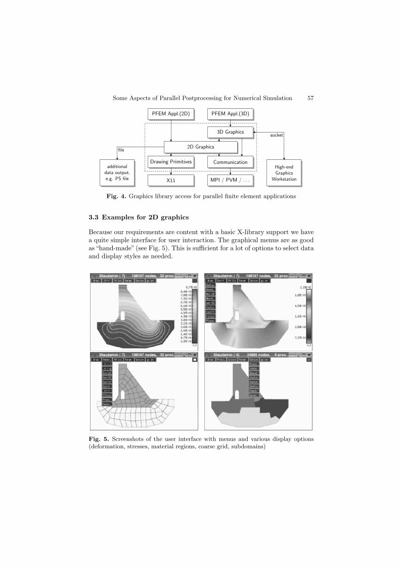
Some Aspects of Parallel Postprocessing for Numerical Simulation 57
X11 MPI / PVM / . . .
Drawing Primitives Communication
2D Graphics
3D Graphics
PFEM Appl.(2D) PFEM Appl.(3D)
additional
data output,
e.g. PS file
High-end
Graphics
Workstation
file
socket
Fig. 4. Graphics library access for parallel finite element applications
3.3 Examples for 2D graphics
Because our requirements are content with a basic X-library support we havea quite simple interface for user interaction. The graphical menus are as goodas “hand-made” (see Fig. 5). This is sufficient for a lot of options to select dataand display styles as needed.
Fig. 5. Screenshots of the user interface with menus and various display options(deformation, stresses, material regions, coarse grid, subdomains)
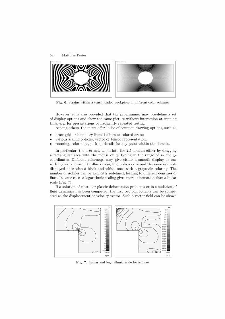
58 Matthias Pester
SFB 393 - TU Chemnitz SFB 393 - TU Chemnitz
Fig. 6. Strains within a tensil-loaded workpiece in different color schemes
However, it is also provided that the programmer may pre-define a setof display options and show the same picture without interaction at runningtime, e. g. for presentations or frequently repeated testing.
Among others, the menu offers a lot of common drawing options, such as
• draw grid or boundary lines, isolines or colored areas;• various scaling options, vector or tensor representation;• zooming, colormaps, pick up details for any point within the domain.
In particular, the user may zoom into the 2D domain either by dragginga rectangular area with the mouse or by typing in the range of x- and y-coordinates. Different colormaps may give either a smooth display or onewith higher contrast. For illustration, Fig. 6 shows one and the same exampledisplayed once with a black and white, once with a grayscale coloring. Thenumber of isolines can be explicitly redefined, leading to different densities oflines. In some cases a logarithmic scaling gives more information than a linearscale (Fig. 7).
If a solution of elastic or plastic deformation problems or in simulation offluid dynamics has been computed, the first two components can be consid-ered as the displacement or velocity vector. Such a vector field can be shown
9.63E-02
0.29
0.48
0.67
0.87
1.1
1.3
1.4
1.6
1.8
2.0
2.2
2.4
2.6
2.8
3.0
3.2
3.4
3.6
3.8
3.9
4.1
4.3
4.5
4.7
7.69E-05
4.8
Eps-V
SFB 393 - TU Chemnitz
9.59E-05
1.49E-04
2.32E-04
3.61E-04
5.61E-04
8.73E-04
1.36E-03
2.11E-03
3.29E-03
5.11E-03
7.95E-03
1.24E-02
1.92E-02
2.99E-02
4.65E-02
7.24E-02
0.11
0.18
0.27
0.42
0.66
1.0
1.6
2.5
3.9
7.69E-05
4.8
Eps-V
SFB 393 - TU Chemnitz
Fig. 7. Linear and logarithmic scale for isolines
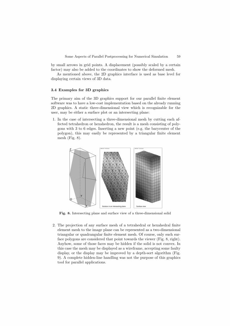
Some Aspects of Parallel Postprocessing for Numerical Simulation 59
by small arrows in grid points. A displacement (possibly scaled by a certainfactor) may also be added to the coordinates to show the deformed mesh.
As mentioned above, the 2D graphics interface is used as base level fordisplaying certain views of 3D data.
3.4 Examples for 3D graphics
The primary aim of the 3D graphics support for our parallel finite elementsoftware was to have a low-cost implementation based on the already running2D graphics. A static three-dimensional view which is recognizable for theuser, may be either a surface plot or an intersecting plane:
1. In the case of intersecting a three-dimensional mesh by cutting each af-fected tetrahedron or hexahedron, the result is a mesh consisting of poly-gons with 3 to 6 edges. Inserting a new point (e.g. the barycenter of thepolygon), this may easily be represented by a triangular finite elementmesh (Fig. 8).
X
Y
Z
O
Solution in an intersecting plane
SFB 393 - TU Chemnitz
Surface view
SFB 393 - TU Chemnitz
Fig. 8. Intersecting plane and surface view of a three-dimensional solid
2. The projection of any surface mesh of a tetrahedral or hexahedral finiteelement mesh to the image plane can be represented as a two-dimensionaltriangular or quadrangular finite element mesh. Of course, only such sur-face polygons are considered that point towards the viewer (Fig. 8, right).Anyhow, some of those faces may be hidden if the solid is not convex. Inthis case the mesh may be displayed as a wireframe, accepting some faultydisplay, or the display may be improved by a depth-sort algorithm (Fig.9). A complete hidden-line handling was not the purpose of this graphicstool for parallel applications.
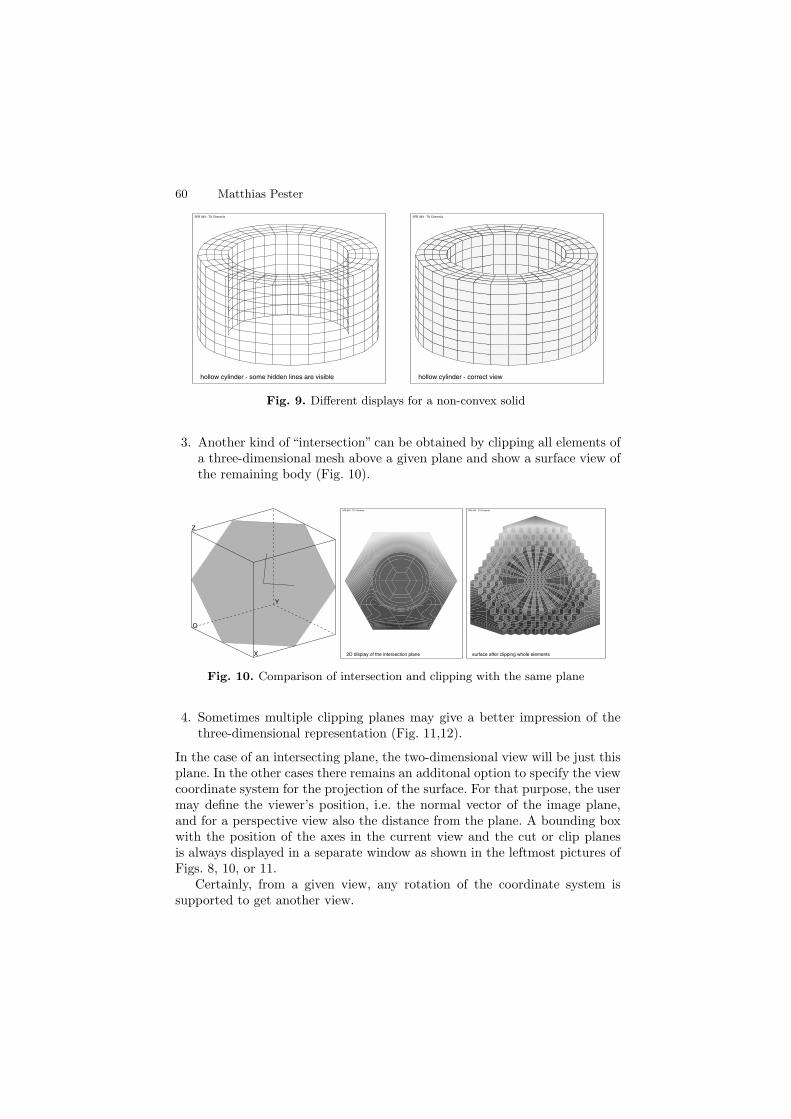
60 Matthias Pester
hollow cylinder - some hidden lines are visible
SFB 393 - TU Chemnitz
hollow cylinder - correct view
SFB 393 - TU Chemnitz
Fig. 9. Different displays for a non-convex solid
3. Another kind of “intersection” can be obtained by clipping all elements ofa three-dimensional mesh above a given plane and show a surface view ofthe remaining body (Fig. 10).
X
Y
Z
O
2D display of the intersection plane
SFB 393 - TU Chemnitz
surface after clipping whole elements
SFB 393 - TU Chemnitz
Fig. 10. Comparison of intersection and clipping with the same plane
4. Sometimes multiple clipping planes may give a better impression of thethree-dimensional representation (Fig. 11,12).
In the case of an intersecting plane, the two-dimensional view will be just thisplane. In the other cases there remains an additonal option to specify the viewcoordinate system for the projection of the surface. For that purpose, the usermay define the viewer’s position, i.e. the normal vector of the image plane,and for a perspective view also the distance from the plane. A bounding boxwith the position of the axes in the current view and the cut or clip planesis always displayed in a separate window as shown in the leftmost pictures ofFigs. 8, 10, or 11.
Certainly, from a given view, any rotation of the coordinate system issupported to get another view.
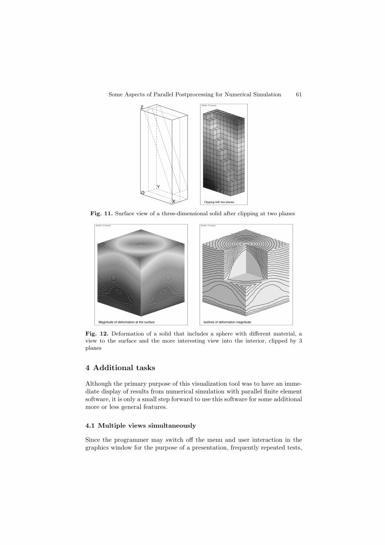
Some Aspects of Parallel Postprocessing for Numerical Simulation 61
X
Y
Z
O
Clipping with two planes
SFB 393 - TU Chemnitz
Fig. 11. Surface view of a three-dimensional solid after clipping at two planes
Magnitude of deformation at the surface
SFB 393 - TU Chemnitz
Isolines of deformation magnitude
SFB 393 - TU Chemnitz
Fig. 12. Deformation of a solid that includes a sphere with different material, aview to the surface and the more interesting view into the interior, clipped by 3planes
4 Additional tasks
Although the primary purpose of this visualization tool was to have an imme-diate display of results from numerical simulation with parallel finite elementsoftware, it is only a small step forward to use this software for some additionalmore or less general features.
4.1 Multiple views simultaneously
Since the programmer may switch off the menu and user interaction in thegraphics window for the purpose of a presentation, frequently repeated tests,
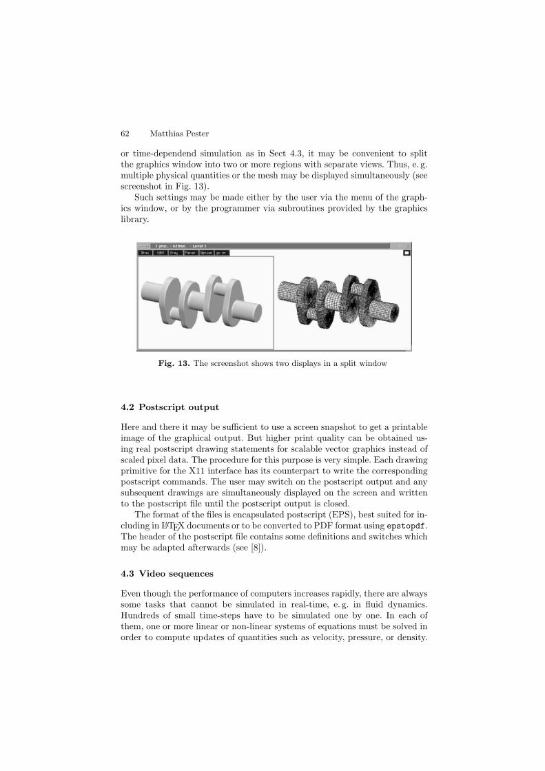
62 Matthias Pester
or time-dependend simulation as in Sect 4.3, it may be convenient to splitthe graphics window into two or more regions with separate views. Thus, e. g.multiple physical quantities or the mesh may be displayed simultaneously (seescreenshot in Fig. 13).
Such settings may be made either by the user via the menu of the graph-ics window, or by the programmer via subroutines provided by the graphicslibrary.
Fig. 13. The screenshot shows two displays in a split window
4.2 Postscript output
Here and there it may be sufficient to use a screen snapshot to get a printableimage of the graphical output. But higher print quality can be obtained us-ing real postscript drawing statements for scalable vector graphics instead ofscaled pixel data. The procedure for this purpose is very simple. Each drawingprimitive for the X11 interface has its counterpart to write the correspondingpostscript commands. The user may switch on the postscript output and anysubsequent drawings are simultaneously displayed on the screen and writtento the postscript file until the postscript output is closed.
The format of the files is encapsulated postscript (EPS), best suited for in-cluding in LATEX documents or to be converted to PDF format using epstopdf.The header of the postscript file contains some definitions and switches whichmay be adapted afterwards (see [8]).
4.3 Video sequences
Even though the performance of computers increases rapidly, there are alwayssome tasks that cannot be simulated in real-time, e. g. in fluid dynamics.Hundreds of small time-steps have to be simulated one by one. In each ofthem, one or more linear or non-linear systems of equations must be solved inorder to compute updates of quantities such as velocity, pressure, or density.
Some Aspects of Parallel Postprocessing for Numerical Simulation 63
In each time-step our visualization tool may produce a single image of thecurrent state on the screen.
At the end one is interested in the behavior of any physical quantity duringthe sequence of time-steps, i. e. to see an animation or a movie.
In order to simplify the simulation process, the visualization may beswitched into a “batch mode”, where the current view is updated automati-cally after each time-step, without user interaction. In most cases, however,the (parallel) numerical simulation together with the computation and displayof graphical output will not be fast enough to see a “movie” on the screen inreal-time.
Therefore, one of the additional tools is a separate program that capturesthe images from the screen (triggered by a synchronizing command of thesimulation program) and saves them as a sequence of image files. After thesimulation has finished the animated solution may be viewed with any suitabletool (xanim, mpegtools).
Refer to http://www.tu-chemnitz.de/~pester/exmpls/ for a list ofexamples with animated solutions.
5 Remarks
This chapter was intended to give only a short overview on visualization soft-ware which was implemented for parallel computing already some years ago,but has also been enhanced more and more over the years. The tools are flex-ible with respect to the underlying hardware and parallel software. Withinthis scope such an overview cannot be complete. For more technical detailsand examples one may refer to the cited papers and Web addresses.
References
1. A. Meyer. A parallel preconditioned conjugate gradient method using domaindecomposition and inexact solvers on each subdomain. Computing, 45 : 217–234,1990.
2. G. Haase, U. Langer, and A. Meyer. Parallelisierung und Vorkonditionierung desCG-Verfahrens durch Gebietszerlegung. In G. Bader et al, editor, Numerische Al-gorithmen auf Transputer-Systemen, Teubner Skripten zur Numerik. B.G. Teub-ner, Stuttgart, 1993.
3. M. Pester. On-line visualization in parallel computations. In W. Borchers,G. Domick, D. Kroner, R. Rautmann, and D. Saupe, editors, Visualization Meth-ods in High Performance Computing and Flow Simulation. VSP Utrecht andTEV Vilnius, 1996. Proceeedings of the International Workshop on Visualiza-tion, Paderborn, 18-21 January 1994.
4. M. Pester. Treating curved surfaces in a 3d finite element program for parallelcomputers. Preprintreihe, TU Chemnitz-Zwickau, SFB393/97-10, April 1997.Available from World Wide Web: http://www.tu-chemnitz.de/sfb393/Files/PS/sfb97e10.ps.gz.
64 Matthias Pester
5. G. Haase, T. Hommel, A. Meyer, and M. Pester. Bibliotheken zur Entwicklungparalleler Algorithmen. Preprint SPC 95 20, TU Chemnitz-Zwickau, Febr. 1996.Available from World Wide Web: http://archiv.tu-chemnitz.de/pub/1998/
0074/.6. M. Pester. Bibliotheken zur Entwicklung paralleler Algorithmen - Basisroutinen
fur Kommunikation und Grafik. Preprintreihe, TU Chemnitz, SFB393/02-01,Januar 2002. Available from World Wide Web: http://www.tu-chemnitz.de/sfb393/Files/PDF/sfb02-01.pdf.
7. NAG’s IRIS Explorer – Documentation. Web documentation, The NumericalAlgorithms Group Ltd, Oxford, 1995–2005. Available from World Wide Web:http://www.nag.co.uk/visual/IE/iecbb/DOC/.
8. M. Pester. Visualization tools for 2D and 3D finite element programs - user’s man-ual. Preprintreihe, TU Chemnitz, SFB393/02-02, January 2002. Available fromWorld Wide Web: http://www.tu-chemnitz.de/sfb393/Files/PDF/sfb02-02.pdf.
Efficient Preconditioners for Special Situationsin Finite Element Computations
Arnd Meyer
Technische Universitat Chemnitz, Fakultat fur Mathematik09107 Chemnitz, [email protected]
1 Introduction
From the very efficient use of hierarchical techniques for the quick solution offinite element equations in case of linear elements, we discuss the generaliza-tion of these preconditioners to higher order elements and to the problem ofcrack growth ,where the introduction to of the crack opening would destroyexisting mesh hierarchies. In the first part of this paper, we deal with thehigher order elements. Here, especially elements based on cubic polynomialsrequire more complicate tasks such as the definition of ficticious spaces andthe Ficticious Space Lemma. A numerical example demonstrates that iterationnumbers similar to the linear case are obtained.
In the second part (Sect. 6 to 10) we present a preconditioner based on achange of the basis of the ansatz functions for efficient simulating the crackgrowth problem within an adaptive finite element code. Again, we are ableto use a hierarchical preconditioner although the hierarchical structure of themesh could be partially destroyed after the next crack opening.
2 Solving finite element equations by preconditionedconjugate gradients
We consider the usual weak formulation of a second order partial differentialequation:
Find u ∈ H1(Ω) (fulfilling Dirichlet–type boundary conditions on ΓD ⊂ ∂Ω)
with a(u, v) = 〈f, v〉 ∀v ∈ H10(Ω) = v ∈ H
1(Ω) : v = 0|ΓD. (1)
For simplicity let Ω be a polygonal domain in Rd (d = 2 or d = 3). So, using
a fine triangulation (in the usual sense)
68 Arnd Meyer
TL = T ⊂ Ω, T are triangles (quadrilaterals) if d = 2,T are tetrahedrons (pentahedrons/hexahedrons) if d = 3,
with the nodes ai (represented by their numbers i), we define a finite dimen-sional subspace V ⊂ H
1(Ω) and define the finite element solution uh ∈ V
froma(uh, v) = 〈f, v〉 ∀v ∈ V ∩H
10(Ω). (2)
(The usual generalizations of approximating a(·, ·) or 〈f, ·〉 or the domain Ωfrom ∪T are straightforward, but not considered here).
Let Φ = (ϕ1(x), . . . , ϕN (x)) be the row vector of the finite element basisfunctions defined in V, then we use the mapping V ∋ u←→ u ∈ R
N by
u = Φu (3)
for each function u ∈ V. With (3) the equation (2) is transformed into thevector space, equivalently to
Kuex = b, (4)
when
K = (a(ϕj , ϕi))Ni,j=1, b = (〈f, ϕi〉)N
i=1 and uh = Φuex.
So we have to solve the linear system (4), which is large but sparse. Wheneverits dimension N exceeds about 103 the problems in using Gaussian eliminationdiverge, so we consider efficient iterative solvers, such as the conjugate gra-dient method with modern preconditioners. The preconditioner in the vectorspace is a symmetric positive definite matrix C−1 (constant over the iterationprocess) for which 3 properties should be fulfilled as best as possible:
P1:The action w := C−1r should be cheap (O(N) arithmetical operations).Here r = Ku− b is the residual vector of an approximate solution u ≈ uex
and w, the preconditioned residual, has to be an approximation to theerror u− uex.
P2:The condition number of C−1K, i.e.
κ(C−1K) = λmax(C−1K)/λmin(C−1K)
should be small, this results in a small number of ∼ κ(C−1K)1/2
iterationsfor reducing a norm of r under a given tolerance ǫ.
P3:The action w = C−1r should work in parallel according to the data distri-bution of all large data (all vectors/matrices with O(N) storage) over theprocessors of a parallel computer.
In the past, preconditioning was a matrix–technique (compare: incompletefactorizations), nowadays the construction of efficient preconditioners usesthe analytical knowledge of the finite element spaces. So, we transform theequation w = C−1r into the finite element space V for further investigationof more complicate higher order finite elements:
Preconditioners in Special Situations 69
Lemma 1. The preconditioning operation w = C−1r on r = Ku− b in RN is
equivalent to the definition of a ‘preconditioned function’ w = Φw ∈ V with
w =
N∑
i=1
ψi〈r, ψi〉
for a special basis Ψ in V.
Proof: With w = C−1r we define w = Φw. For a given u ∈ RN , we have
u = Φu ∈ V and define the ‘residual functional’ r ∈ H−1(Ω) with
a(u, v)− 〈f, v〉 = 〈r, v〉 ∀v ∈ H10(Ω).
In the PCG algorithm, we have the values 〈r, ϕi〉 within our residual vectorr:
r = Ku− b =(∑
a(ϕj , ϕi)uj − 〈f, ϕi〉)N
i=1
= (a(u, ϕi)− 〈f, ϕi))Ni=1 = (〈r, ϕi〉)N
i=1
So, w = Φw = ΦC−1r can be written with any factorization C−1 = FFT
(square root of C−1 or Cholesky decomposition etc.) as
w = ΦFFT r =N∑
i=1
ψi〈r, ψi〉,
whenever Ψ = (ψ1 . . . ψN ) = ΦF is another basis in V, transformed with theregular (N ×N)–matrix F .
Remark 1: If no preconditioning is used, we have C−1 = F = I, thedefinition of w is
w =
N∑
i=1
ϕi〈r, ϕi〉
with our nodal basis Φ.
Remark 2: The well–known hierarchical preconditioner due to [16] (seenext section) constructs the matrix F directly from the basis transformationof nodal basis functions Φ into hierarchical base functions Ψ and the actionw := C−1r is indeed
w := FFT r.
70 Arnd Meyer
3 Basic facts on hierarchical and BPX preconditionersfor linear elements
Let the triangulation TL be the result of L refinement steps starting from agiven coarse mesh T0. For simplicity let each triangle T ′ in Tl−1 be subdividedinto 4 equal subtriangles of Tl. Then the mesh history is stored within a listof nodal numbers, where each new node ai = 1
2 (aj +ak) from subdividing theedge (aj , ak) in Tl−1 is stored together with his ‘father’ nodes:
(i, j, k) =(Son, Father1, Father2).
This list is ordered from coarse to fine due to the history. Note that in thequadrilateral case this list contains (Son, Father1, Father2) if an edge is sub-divided, but additionally
(Son, Father1, Father2, Father3, Father4)
with the ‘Son’ as interior node and all four vertices of a quadrilateral subdi-vided into 4 parts. With this definition we have the finite element spaces Vl
belonging to the triangulation Tl equipped with the usual nodal basis Φl
Vl = spanΦl, l = 0, . . . , L.
All functions in this basis are piecewise (bi–)linear with respect to Tl. From
V0 ⊂ V1 ⊂ · · · ⊂ VL, (5)
we can define a hierarchical basis ΨL in VL recursively:Let Ψ0 = Φ0 and Ψl−1 the hierarchical basis in Vl−1 = spanΨl−1 = spanΦl−1,then we define
Ψl = (Ψl−1
...Φnewl ) (6)
where Φnewl contains all ‘new’ nodal basis functions of Vl belonging to nodes
ai that are new (‘Sons’) in Tl (not existent in Tl−1).For l = L, we have VL = spanΨL = spanΦL, so another basis additionally toΦL is defined and there exists a regular (N ×N)–Matrix F with ΨL = ΦLFwhich is used in our preconditioning procedure as considered in Sect. 2.From [16] the following facts are derived:
P2 is fulfilled with κ(C−1K) = O(L2) = O(| log h|2) from the good conditionof the ‘hierarchical stiffness matrix’ KH = FTKF (κ(KH) = κ(C−1K)),which is a consequence of ‘good’ angles between the subspaces Vl−1 and(Vl − Vl−1).
P1 is fulfilled from the recursive refinement formula: Consider the spaces Vl−1
and Vl with the bases Φl−1 and Φl (dim Vl = Nl). Then from Vl−1 ⊂ Vl
there is an (Nl ×Nl−1)–Matrix Pl−1 with
Φl−1 = ΦlPl−1. (7)
Preconditioners in Special Situations 71
Here Pl−1 is explicitly known
Pl−1 =
I· · ·Pl−1
(8)
from
ϕ(l−1)i = ϕ
(l)i +
1
2
∑
j∈N (i)
ϕ(l)j . (9)
(The sum runs over all ‘new’ nodes j that are neighbors of i forming theset N (i).)That is, Pl−1 hat values 1
2 at position (j, i) iff j is ‘Son’ of i oran edge (i, i′) from Tl−1 was subdivided into (i, j) and (i′, j) in Tl.So, the value 1
2 occurs exactly twice in each row of Pl−1.
From this definition for all l = 1, . . . , L follows that F is a product of transfor-mations from level to level, from which the matrix vector multiply w := FFT rbecomes very cheap according to the following two basic algorithms:
A1: y := FT r is done by:1. y := r2. for all entries within the list (backwards) do:
y(Father1) := y(Father1) + 12y(Son)
y(Father2) := y(Father2) + 12y(Son)
A2: w := Fy is done by:1. w := y2. for all entries within the list do:
w(Son) := w(Son) +1
2(w(Father1) + w(Father2))
Note: In the quadrilateral case sometimes 4 fathers exist then 12 is to be
replaced by 14 due to another refinement equation.
Remark 1: This preconditioner works perfectly in a couple of applicationsin 2D. Basically it has been successfully used for simple potential problems,but a generalization to linear elasticity problems (plane stress or plane strain2D) is simple. Here, we use this technique for each single component of thevector function u ∈ (H1(Ω))2. The condition number κ(C−1K) is enlarged bythe constant from Korn’s inequality.
Remark 2: For 3D problems, a growing condition number κ(C−1K) =O(h−1) would appear. To overcome this difficulty, the BPX preconditionerhas to be used [3, 11]. According to (7) we have
72 Arnd Meyer
Φl = ΦLQl ∀l = 0, . . . , L
Ql = PL−1 · . . . · Pl is (N ×Nl) and QL = I.(10)
Then the BPX preconditioner is defined as
w = C−1r =
L∑
l=0
Nl∑
i=1
ϕ(l)i 〈r, ϕ
(l)i 〉 · dl
i (11)
which is (from Sect. 2) equivalent to:
w =L∑
l=0
QlDlQTl r. (12)
Here, Dl = diag(dl1, . . . , d
lNl
) are scale factors, which can be chosen as 2(d−2)l
or as inverse main diagonal entries of the stiffness matrices Kl = QTl KQl
belonging to Φl.For this preconditioner the fact κ(C−1K) ≤ const (independent of h) can beproven and the algorithm for (12) is similar to (A1) and (A2).
4 Generalizing hierarchical techniquesto higher order elements
From the famous properties of the preconditioning technique in Sect. 3, weshould wish to construct similar preconditioners for higher order finite ele-ments and especially for shell and plate elements.
We propose the same nested triangulation as in Sect. 3: T0, . . . , TL. Let nl
be the total number of nodes in Tl, then in Sect. 3 we had Nl = nl (it wasone degree of freedom per node). Now this is different, usually Nl > nl (atleast for l = L, where the finite element space VL = V for approximating ourbilinear form is defined).
For using hierarchical–like techniques we have 3 possibilities:
Technique 1: For some kind of higher order elements, we define the finiteelement spaces Vl on each level and obtain nested spaces
V0 ⊂ V1 ⊂ . . . ⊂ VL.
In this case the same procedure as in Algorithms A1/A2 can be used, but dueto a more complicate refinement formula (instead of (9)), the algorithms areto be adapted.
Example 1: Bogner–Fox–Schmidt–elements on quadrilaterals (with bicubicfunctions and 4 degrees of freedom per node), see [13,14].
Preconditioners in Special Situations 73
Technique 2: Usually we cannot guarantee that the spaces Vl are nested(i.e. Vl−1 ⊂ Vl), but our finest space V = VL belonging to the triangulationTL contains all piecewise linear functions on TL. So we have the nested spaces
V(1)0 ⊂ . . . ⊂ V
(1)L ⊂ VL, when V
(1)l are defined of the piecewise linear functions
on Tl (as in Sect. 3). Then we have to represent VL = V(1)L
+· WL (direct sum)
and prove that γ = cos ∠(V(1)L ,WL) < 1. This angle is defined from the a(·, ·)
energy–inner product
γ2 = supa2(u, v)
a(u, u)a(v, v), where (13)
the supremum is taken over all u ∈ V(1)L and v ∈WL. If γ < 1 (independent of
h), the preconditioner works as in Sect. 3 for l = 0, . . . , L (and linear elements:A1/A2) and additionally there is one transformation from the nodal basis ΦL
of VL into the hierarchical basis (Φ(1)L
...ΦnewL ) of (V
(1)L
+· WL) and back. Againwe have to calculate a special refinement formula for this last step:
Φ(1)L = ΦLPL. (14)
Here, PL has another structure as Pl(l < L) from Sect. 3. The entries of PL
are defined fromϕ
(1)i = ϕhigher
i +∑
j∈N(i)
αijϕhigherj , (15)
where Φ(1)L = (ϕ
(1)1 , . . . , ϕ
(1)nL) are the piecewise linear basis functions and
ϕhigherj the finite element basis functions that span VL (for example piece-
wise polynomials of higher order).
Example 2: VL = V(2)L (piecewise quadratic polynomials on 6–node trian-
gles). Here, αij = 12 iff i is vertex node of TL and j the node on the midpoint
of an edge (ai, ai′). From αij = 12 follows that Algorithm A1/A2 can be used
without change (one level more, all edge nodes are ‘sons’ of the vertex nodesof this edges).
Example 3: VL = V(2)L (piecewise biquadratic polynomials on 9–node
quadrilaterals). Here,
αij =
12 j midpoint of an edge (i, i′)14 j interior node
Again Algorithm A1/A2 works without change, one level more.
Example 4: VL = V(2,red)L (reduced biquadratic polynomials on 8–node
quadrilaterals).Here, αij = 1
2 , again use Algorithm A1/A2.
74 Arnd Meyer
Example 5: VL = V(3,red)L (piecewise reduced cubic polynomials on tri-
angles, the cubic bubble is removed such that all quadratic polynomials areincluded).This example has to be considered, because this space occurs as fictitiousspace in Technique 3. Here, we define the following functions:u(x) ∈ VL is a reduced cubic polynomial on each T ∈ TL (defined by 9 valueson the vertices of T ).We choose ui = u(ai) and ui,j = ∂u
∂sij|ai
, the tangential derivatives along the
edges of T : aij = aj − ai, sij = aij/|aij |.Globally, we have |N (i)| + 1 degrees of freedom at each node ai: ui = u(ai)and ui,j = ∂u
∂sij|ai∀j ∈ N (i). From this definition, we easily find
ϕ(1)i (x) = ϕ
(3)i (x) +
∑
j∈N (i)
1
|aij |(ϕj,i(x)− ϕi,j(x)). (16)
Here, ϕ(3)i (x) is the finite element basis function with
ϕ(3)i (aj) = δij and ∇ϕ(3)
i (aj) = (0, 0)T ∀i, j (17)
(with support of all T around ai) and ϕi,j(x) fulfills
ϕi,j(ak) = 0∀i, j, k, ∂
∂sijϕi,j(ai) = 1 (18)
∂
∂sikϕi,j(ai) = 0 for all edges (i, k) = (i, j),
so the support are two triangles that share the edge (i, j).
In the splitting V(3,red)L = V
(1)L + WL, WL is spanned by all functions ϕi,j(x).
Technique 3: There are examples, where neither the spaces Vl are nested,
nor piecewise linear functions V(1)L are contained within the finest space VL.
Here, we can use the Fictitious Space Lemma (see [9,11]) for the constructionof a preconditioner which is written as
C−1 = RC−1R∗, (19)
if a fictitious space V exists (in general of higher dimension than VL) havinga good preconditioner C−1. The key is the definition of a restriction operator
R : V→ VL
with small energy norm.
Example 6: For more complicate plate analysis, the space VHC of Hermite–
triangles is used (DKT–elements, HCT–elements). Here u ∈ VHC is again a
Preconditioners in Special Situations 75
reduced cubic polynomial on each T ⊂ TL, but we use globally 3 degrees offreedom per node: ui = u(ai) and Θi = ∇u(ai).Here, ∇u is discontinuous on the edges, but continuous on each node ai. From
this property the spaces cannot be nested and the functions in V(1)L have
discontinuous gradients on all vertices ai, so V(1)L ⊂ V
HC .From V
HC ⊂ V(3,red), we may define a restriction operator
R : V(3,red)L → VL = V
HC
and use the preconditioner for V(3,red)L from Example 5 for defining C−1, which
leads to a good preconditioner for this space VHC . The definition of R is not
unique, we use an easy choice, some kind of averaging of ∂u∂sij|ai
to ∇u(ai):
Let u ∈ V(3,red)L be represented by
ui = u(ai) and ui,j =∂u
∂sij|ai
(∀i,∀j ∈ N (i) )
then we define u = Ru ∈ VHC with ui = u(ai) and Θi = ∇u(ai) from
Θi =1
miSi ui (ui = (ui,j) ∀j ∈ N (i) ).
The (2×mi)−matrix Si contains all normalized vectors sij for all edges meet-ing ai and mi = |N (i)|. So,
Θi =1
mi
∑
j∈N (i)
sij ·∂u
∂sij|ai
=1
mi
∑ui,jsij (20)
5 Numerical examples to the above preconditioners
Let us demonstrate the preconditioners proposed in Sect. 4 at one examplethat allows some of the finite elements discussed in Example 1 to Example 6.We chooseΩ as a rectangle with prescribed Dirichlet type boundary conditionsand solve a simple Laplace equation
−∆u = 0 in Ωu = g on ∂Ω,
hence, a(u, v) =∫Ω
(∇u) · (∇v)dΩ and we use the following discretization:
(a) piecewise linear functions (VL = V(1)L )
on a triangular mesh (3–node–triangles)
(b) piecewise bilinear functions (VL = V(1)L )
on a quadrilateral mesh (4–node–quadrilaterals)
76 Arnd Meyer
(c) piecewise quadratic functions (VL = V(2)L )
on a triangular mesh (6–node–triangles)
(d) piecewise biquadratic functions (VL = V(2)L )
on quadrilaterals (9–node–quadrilaterals)
(e) piecewise reduced quadratic functions (VL = V(2,red)L )
on quadrilaterals (8–node–quadrilaterals)(f) piecewise reduced cubic functions (VL = V
HC)on a triangular mesh (Hermite cubic triangles)
The preconditioners for cases (a) to (e) were simply described in Examples 1to 4 in Sect. 4. We will give the matrix representation for the preconditionerof case (f) from combining Examples 5 and 6:For VL = V
HC , we have to solve
a(u, v) = 〈f, v〉 ∀v ∈ VL ∩H10(Ω)
in solvingKuex = b.
Here u = Φu is represented by ui = u(ai) and Θi = ∇u(ai), so u ∈ R3n.
The preconditioner C−1 from Sect. 2 is an operator which maps the residualfunctional r(u) to the preconditioned function w. According to the fictitiousspace lemma, we set
C−1 = RC−1R∗
with R : V = V(3,red)L → VL = V
HC as in Example 6. In the fictitious
space V, we use the preconditioner of Example 5. From Example 5 the matrixrepresentation of this preconditioner is
C−1 = QL
(FFT
O
O I
)QT
L (21)
with F from Sect. 2. Here, QL transforms the basis (Φ(3)...Φ(edge)) of the cubic
functions in V(3,red) into the hierarchical basis (Φ(1)
...Φ(edge)).
Φ(1) = (ϕ(1)1 , . . . , ϕ
(1)n ) piecewise linear functions
Φ(3) = (ϕ(3)1 , . . . , ϕ
(3)n ) piecewise reduced cubic
with property (17)Φ(edge) = (ϕi,j)∀ edges (i, j) at node i piecewise reduced cubic
with property (18)
So,
QL =
I
... O
PL
... I
(22)
and entries of PL are found in (16). Combining this with Example 6, we have
Preconditioners in Special Situations 77
C−1 = RQL
(FFT
O
O I
)QT
LRT , (23)
when R is the matrix representation of R. The implementation of C−1 is thefollowing algorithm (note that RQL is done at once for saving storage, this isa (3n× 3n)–matrix).The preconditioner C−1 acts on a residual vector r ∈ R
3n (n = nL) with theentries
ri = 〈r, ϕi,0〉 and Θi =
(〈r, ϕi,1〉〈r, ϕi,2〉
)
defined with the basis functions (ϕi,α) in VHC :
ϕi,0(aj) = δij ϕi,1(aj) = ϕi,2(aj) = 0∇ϕi,0(aj) = (0, 0)T ∇ϕi,1(aj) = δij(1, 0)T
∇ϕi,2(aj) = δij(0, 1)T .
Analogously, the result w = C−1r contains entries wi and Θi (for w(ai) and∇w(ai)). From the definition
C−1 = RC−1RT = RQL
(FFT
O
O I
)QT
LRT
we have to implement the matrix-vector-multiply
(RQL)T r
and w = RQLy, which is done at once for saving storage, i.e. there is noneed to store the (approximately 7n) values ui,j = sTijΘi. This is contained in
Algorithms B1 (for y := (RQL)T r) and B2 (for w := RQLy).
Algorithm B1: for each edge (i, j) do
∣∣∣∣yi := ri − aT
ij(Θi + Θj)/|aij |2yj := rj + aT
ij(Θi + Θj)/|aij |2
Algorithm B2: for each edge (i, j) do
∣∣∣∣Θi := Θi + aij(a
TijΘi + wj − wi)/|aij |2
Θj := Θj + aij(aTijΘj + wj − wi)/|aij |2
Θi are evaluated from a Jacobi–preconditioning on the input Θi, wi are theresults of Algorithms A1/A2 on the n–vector y.The hierarchical–like preconditioners for the elements (a) to (f) require a verysmall number of PCG–iterations as presented in the following Table 1.
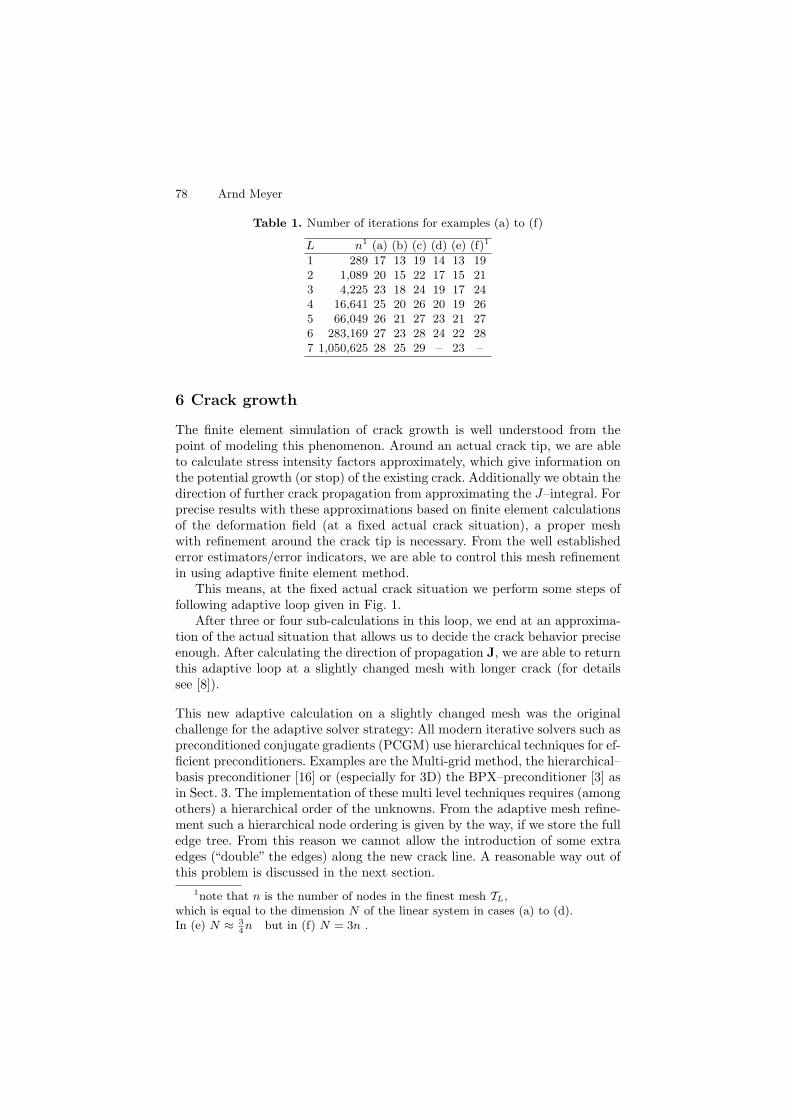
78 Arnd Meyer
Table 1. Number of iterations for examples (a) to (f)
L n1 (a) (b) (c) (d) (e) (f)1
1 289 17 13 19 14 13 192 1,089 20 15 22 17 15 213 4,225 23 18 24 19 17 244 16,641 25 20 26 20 19 265 66,049 26 21 27 23 21 276 283,169 27 23 28 24 22 287 1,050,625 28 25 29 – 23 –
6 Crack growth
The finite element simulation of crack growth is well understood from thepoint of modeling this phenomenon. Around an actual crack tip, we are ableto calculate stress intensity factors approximately, which give information onthe potential growth (or stop) of the existing crack. Additionally we obtain thedirection of further crack propagation from approximating the J–integral. Forprecise results with these approximations based on finite element calculationsof the deformation field (at a fixed actual crack situation), a proper meshwith refinement around the crack tip is necessary. From the well establishederror estimators/error indicators, we are able to control this mesh refinementin using adaptive finite element method.
This means, at the fixed actual crack situation we perform some steps offollowing adaptive loop given in Fig. 1.
After three or four sub-calculations in this loop, we end at an approxima-tion of the actual situation that allows us to decide the crack behavior preciseenough. After calculating the direction of propagation J, we are able to returnthis adaptive loop at a slightly changed mesh with longer crack (for detailssee [8]).
This new adaptive calculation on a slightly changed mesh was the originalchallenge for the adaptive solver strategy: All modern iterative solvers such aspreconditioned conjugate gradients (PCGM) use hierarchical techniques for ef-ficient preconditioners. Examples are the Multi-grid method, the hierarchical–basis preconditioner [16] or (especially for 3D) the BPX–preconditioner [3] asin Sect. 3. The implementation of these multi level techniques requires (amongothers) a hierarchical order of the unknowns. From the adaptive mesh refine-ment such a hierarchical node ordering is given by the way, if we store the fulledge tree. From this reason we cannot allow the introduction of some extraedges (“double” the edges) along the new crack line. A reasonable way out ofthis problem is discussed in the next section.
1note that n is the number of nodes in the finest mesh TL,which is equal to the dimension N of the linear system in cases (a) to (d).In (e) N ≈ 3
4n but in (f) N = 3n .

Preconditioners in Special Situations 79
refine / coarsen
marked elements
calculate element matrices
for new elements
solve the linear system
calculate error indicatorsfrom last solution and
for refining / coarseningmark elements
Fig. 1. The adaptive solution loop
7 Data structure for maintaining hierarchies
The idea of the extension of the crack line is given in [8]. We subdivide theexisting edges that cut the crack line at the cutting point. Then the usual meshrefinement creates (during “red” or “green” subdivision of some elements) newedges along the crack line together with a proper slightly refined mesh andthe correct hierarchies in the new edge tree.
So, there are no“double”edges along the crack line. For defining the doublenumber of unknowns at the so called “crack–nodes”, we introduce a copy ofeach crack–node and call the old one “–”-node on one side of the crack andthe other “+”-node at the other side. Now, the hierarchical preconditioner
P
new P
+
+
+
+
+ +
+
+
+
−
− −−
−
−
−−
−
−
+
−
Fig. 2. Mesh handling after crack extension from the old crack tip P to “new P”
80 Arnd Meyer
can access from its edge tree information only the usual and the “–”-valuesbut never the new additional “+”-values. An efficient preconditioner has tocombine both informations as it was expected in [8] from a simple averagingtechnique of the results of two preconditioners (first with usual and“–”-values,then with usual and “+”-values). This simple approach never can lead toa spectrally equivalent preconditioner which is clearly seen in relative highnumbers of PCG–iterations. Here, another approach with a basis change anda domain decomposition like method will be given in the next chapter.
8 Two kind of basis functions for crack growthfinite elements
The fact that we have a coherent continuum before the growth of the crackthat changes into a slit–domain after growing requires a special finite elementtreatment. One possibility is the construction of a new mesh after crackgrowing, where the new free crack shores are usual free boundaries (with zerotraction boundary condition). This is far away from being efficient because wehave a mesh from Sect. 6 and the error indicators will drive the future refine-ment and coarsening to the required mesh for good approximating this newsituation. So, we start to work with the existing mesh with double degreesof freedom at the crack nodes.
From the technique in [8], the crack–line in the undeformed domain is rep-resented by some edges. Each edge refers to its end–nodes. For the calculationof the crack opening these nodes carry twice as much degrees of freedom andare called “crack–nodes”.
Let the total number of nodes N = n+ d of the actual mesh be split inton usual nodes and d crack–nodes. The degrees of freedom of the crack–nodesare called “–”-values on one shore of the crack and (different) “+”-values onthe other shore. A finite element which contains at least one crack–node iscalled “–”-element, if it refers to “–”-values (lays at “–”-side of the crack) andconversely, a “+”-element refers to “+”-values and lays at the other side of thecrack–line (as indicated in Fig. 2).
From the usual element by element calculation of the stiffness matrix,using these 2d double unknowns along the d crack–nodes, we understand theresulting stiffness matrix as usual finite element matrix that belongs to thefollowing basis of (vector) ansatz functions:
Φ =(ϕ1I , . . . , ϕnI, ϕ
−n+1I , . . . , ϕ
−n+dI, ϕ
+n+1I , . . . , ϕ
+n+dI
).
Here, we write ϕkI = (ϕke1
...ϕke2) to specify the two usual vector ansatzfunctions. Moreover, ϕk (k = 1 . . . n) denotes a usual hat–function on theusual node k. In contrast to that, ϕ−
n+j and ϕ+n+j are half hat functions with
Preconditioners in Special Situations 81
its support around the crack–node (n + j) at the “–”-elements (“+”-elementsresp.) only. (If a usual node k lays on the remaining free boundary of thedomain, the function ϕk is such a “half” hat function as well). The totalnumber of ansatz functions is 2 · (n + d + d), which is the dimension of theresulting stiffness matrix K.
For the efficient preconditioning of this matrix K, we introduce anotherbasis of possible ansatz functions, that span the same 2(n+ 2d)–dimensionalfinite element space:
Φ = (ϕ1I , . . . , ϕnI, ϕn+1I , . . . , ϕn+dI, ϕn+1I , . . . , ϕn+dI).
Here, ϕn+j is the usual full (continuous) hat function at the node (n+ j) andϕn+j is the product of ϕn+j with the Heaviside function of the crack–line.This means:
ϕn+j := ϕ−n+j + ϕ+
n+j (a.e.)
ϕn+j := ϕ−n+j − ϕ+
n+j (a.e.) .(24)
Hence, ϕn+j has a jump from −1 to +1 over the crack–line at the crack–node(n+ j).
Theoretically, we can use K, the stiffness matrix of Φ instead of K for thesame finite element computation of the new crack opening. Note the followingdifferences between these two basis definitions:
Advantages of Φ:
• usual element routines• usual post–processing (direct calculation of the displacements of both crack
shores)• usual error estimators / error indicators (at the crack the same data as at
free boundaries)
Disadvantage of Φ:
• requires special preconditioner for K
For the basis Φ the reverse properties are true. The use of Φ would requiresome special treatment in element routines, post–processing and a new errorcontrol.
For K an efficient preconditioner can be found, so by use of the basistransformation (24) we construct an efficient preconditioner for K as well.Obviously
Φ = ΦD
with the block–diagonal matrix
D = blockdiag (D1, D2),
82 Arnd Meyer
whereD1 = I, (2n× 2n),
and
D2 =
(I II −I
), (2 · (2d)× 2 · (2d)).
This leads toK = DKD. (25)
So, if C is a good preconditioner for K, then C = D−1CD−1 is as good forK.
9 An efficient DD–preconditioner for K
From the special structure of the matrix K a domain decomposition approachleads to a very efficient preconditioner. Let us recall the structure of K fromthe definition of the basis Φ:
K =
A B− B+
(B−)T T−O
(B+)TO T+
with the blocks:A (2n × 2n) of the energy inner products of all usual basis functions ϕiek
with itself,T− (2d× 2d) of the energy inner products of all ϕ−
n+iek with itself,
T+ (2d× 2d) of the energy inner products of all ϕ+n+iek with itself and
B−, B+ contain all energy inner products of ϕiek(i ≤ n) with ϕ−n+jel (resp.
ϕ+n+jel).
No “+”-node is coupled to a “–”-node, this leads to both zero blocks (thecrack-tip is understood as “usual node”).
If we perform the transformation (25), the new matrix K possesses a muchmore simple structure:
K =
A B− +B+ B− −B+
sym. T− + T+ T− − T+
sym. T− − T+ T− + T+
(26)
which is abbreviated as
K =
(A0 BBT T
)
with A0 the leading 2(n+ d)–block and
B =
(B− −B+
T− − T+
), T = T− + T+.
Preconditioners in Special Situations 83
Then the matrix A0 is defined from all energy inner products of all first 2(n+d)usual hat functions of the basis Φ. Hence, A0 is the usual stiffness matrix forthe actual mesh without any crack opening.All the n+d nodes are represented in a hierarchical structure of the edge–tree,so any kind of multi–level preconditioners can easily be applied for precondi-tioning A0.Especially the most simple hierarchical–basis preconditioner as explained inSect. 3 (for details see [16]) would be very cheap but effective.A resulting good preconditioner for the whole matrix follows from the finestructure of T :If all crack–nodes are ordered in a 1–dimensional chain, then T has block–tridiagonal form for linear elements or block–pentadiagonal form for quadraticelements. Hence, the storage of the sub block T (upper triangle) can bearranged with
8d values (linear elements, fixed bandwidth scheme),7d values (linear elements, variable bandwidth scheme),12d values (quadratic elements, fixed bandwidth scheme) or9d values (quadratic elements, variable bandwidth scheme),
and the Cholesky decomposition of T is of optimal order of complexity dueto the fixed bandwidth.This is exploited best in a domain decomposition–like preconditioner, whichresults from a simple block factorization of K:
K =
(I BT−1
O I
)(S O
O T
)(I O
T−1BT I
)
with the Schur–complement matrix
S = A0 −BT−1BT .
The inverse of K can be approximated by the inverse preconditioner C−1:
C−1 =
(I O
−T−1BT I
)(C−1
0 O
O T−1
)(I −BT−1
O I
),
when C0 represents a good preconditioner for S. Note that all other inverts areexact (especially T−1 ), so the spectrum of C−1K coincides with the spectrumof C−1
0 S and additional unities. With proper scaling, we have C for K as goodas C0 for S. The Schur complement is a rank–2d–perturbation of A0, so weuse the same preconditioner C0 for S as it was explained for A0. The resultingpreconditioner for K follows from (24),(25) as the formula
C−1 = D
(I 0
−T−1BT I
)(C−1
0 O
O I
)(I −BT−1
0 T−1
)D.
For the action w := C−1r within the PCGM iterations, we need once theaction of the (hierarchical) preconditioner C0 and twice a solver with T , theremaining effort is a multiplication with parts of the stiffness matrix only,which determines a preconditioner of optimal complexity.
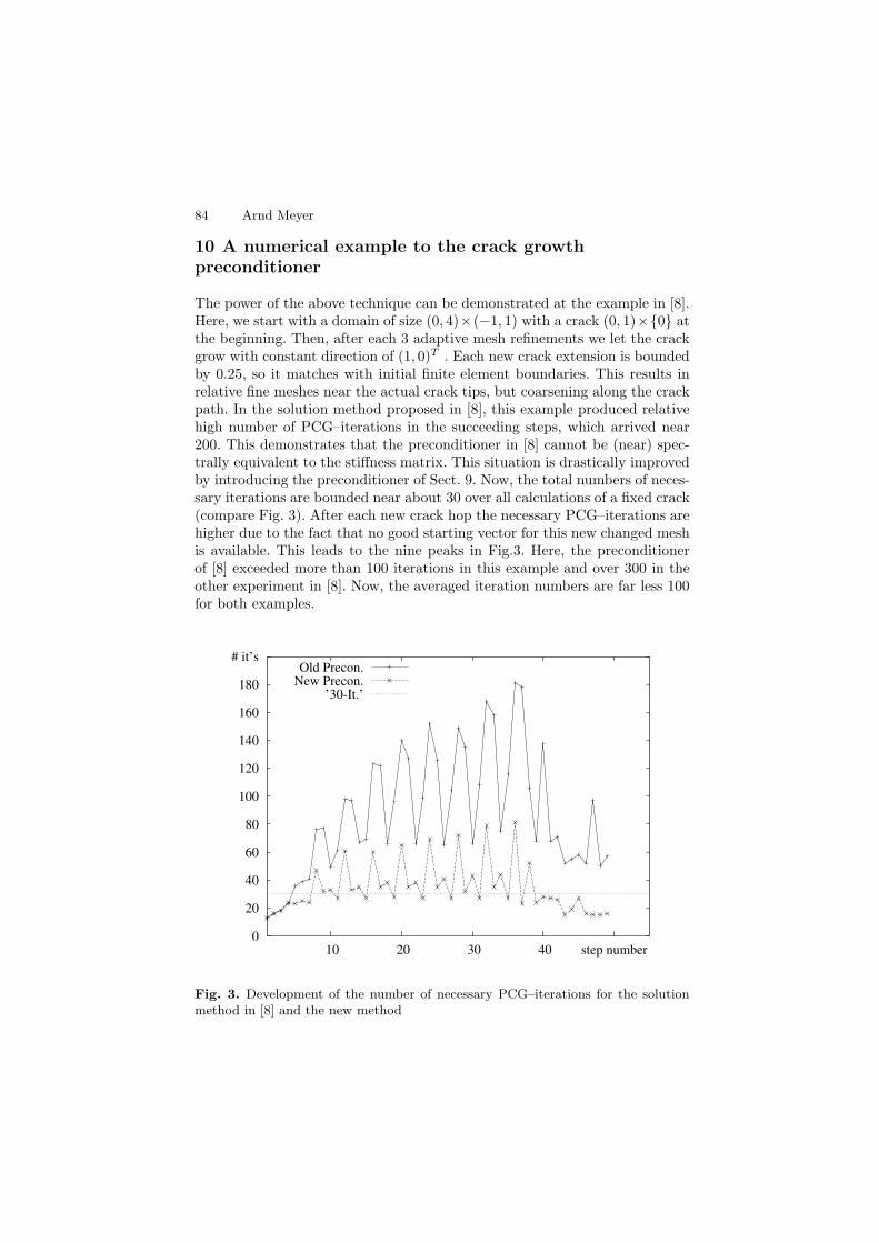
84 Arnd Meyer
10 A numerical example to the crack growthpreconditioner
The power of the above technique can be demonstrated at the example in [8].Here, we start with a domain of size (0, 4)×(−1, 1) with a crack (0, 1)×0 atthe beginning. Then, after each 3 adaptive mesh refinements we let the crackgrow with constant direction of (1, 0)T . Each new crack extension is boundedby 0.25, so it matches with initial finite element boundaries. This results inrelative fine meshes near the actual crack tips, but coarsening along the crackpath. In the solution method proposed in [8], this example produced relativehigh number of PCG–iterations in the succeeding steps, which arrived near200. This demonstrates that the preconditioner in [8] cannot be (near) spec-trally equivalent to the stiffness matrix. This situation is drastically improvedby introducing the preconditioner of Sect. 9. Now, the total numbers of neces-sary iterations are bounded near about 30 over all calculations of a fixed crack(compare Fig. 3). After each new crack hop the necessary PCG–iterations arehigher due to the fact that no good starting vector for this new changed meshis available. This leads to the nine peaks in Fig.3. Here, the preconditionerof [8] exceeded more than 100 iterations in this example and over 300 in theother experiment in [8]. Now, the averaged iteration numbers are far less 100for both examples.
0
20
40
60
80
100
120
140
160
180
# it’s
10 20 30 40 step number
Old Precon.New Precon.
’30-It.’
Fig. 3. Development of the number of necessary PCG–iterations for the solutionmethod in [8] and the new method
Preconditioners in Special Situations 85
References
1. E. Bansch: Local mesh refinement in 2 and 3 dimensions. IMPACT of Com-puting in Science and Engineering 3, pp. 181–191, 1991.
2. J. H. Bramble, J. E. Pasciak, A. H. Schatz, ”The Construction of Preconditionersfor Elliptic Problems by Substructuring” I – IV, Mathematics of Computation,47:103–134,1986, 49:1–16,1987, 51:415–430,1988, 53:1–24,1989.
3. I. H. Bramble, J. E. Pasciak, J. Xu, Parallel Multilevel Preconditioners, Math.Comp., 55:1-22,1990.
4. G. Haase, U. Langer, A. Meyer,The Approximate Dirichlet Domain Decomposi-tion Method, Part I: An Algebraic Approach, Part II: Application to 2nd-orderElliptic B.V.P.s, Computing, 47:137-151/153-167,1991.
5. G. Haase, U. Langer, A. Meyer, Domain Decomposition Preconditioners withInexact Subdomain Solvers, J. Num. Lin. Alg. with Appl., 1:27-42,1992.
6. G. Haase, U. Langer, A. Meyer, S.V. Nepommnyaschikh, Hierarchical ExtensionOperators and Local Multigrid Methods in Domain Decomposition Precondi-tioners, East-West J. Numer. Math., 2:173-193,1994.
7. A. Meyer, A Parallel Preconditioned Conjugate Gradient Method Using DomainDecomposition and Inexact Solvers on Each Subdomain, Computing, 45:217-234,1990.
8. A. Meyer, F.Rabold, M.Scherzer: Efficient Finite Element Simulation of CrackPropagation Using Adaptive Iterative Solvers, Commun.Numer.Meth.Engng.,22,93-108, 2006. Preprint-Reihe des Chemnitzer Sonderforschungsbereiches 393,Nr.: 04-01, TU Chemnitz, 2004.
9. S.V. Nepommnyaschikh, Ficticious components and subdomain alternatingmethods, Sov.J.Numer.Anal.Math.Model., 5:53-68,1991.
10. Rolf Rannacher and Franz-Theo Suttmeier: A feed-back approach to error con-trol in finite element methods: Application to linear elasticity. Reaktive Stro-mungen, Diffusion und Transport SFB 359, Interdiziplinares Zentrum fur Wis-senschaftliches Rechnen der Universitat Heidelberg, 1996.
11. P.Oswald, Multilevel Finite Element Approximation: Theory and Applications,Teubner Skripten zur Numerik, B.G.Teubner Stuttgart 1994.
12. M. Scherzer and A. Meyer: Zur Berechnung von Spannungs- und Deformations-feldern an Interface-Ecken im nichtlinearen Deformationsbereich auf Parallel-rechnern. Preprint-Reihe des Chemnitzer Sonderforschungsbereiches 393, Nr.:96-03, TU Chemnitz, 1996.
13. M.Thess, Parallel Multilevel Preconditioners for Thin Smooth Shell Finite Ele-ment Analysis, Num.Lin.Alg.with Appl., 5:5,401-440,1998.
14. M.Thess, Parallel Multilevel Preconditioners for Thin Smooth Shell Problems,Diss.A, TU Chemnitz,1998.
15. P. Wriggers: Nichtlineare Finite-Element-Methoden. Springer, Berlin, 2001.16. H. Yserentant, Two Preconditioners Based on the Multilevel Splitting of Finite
Element Spaces, Numer. Math., 58:163-184,1990.

Nitsche Finite Element Method for EllipticProblems with Complicated Data
Bernd Heinrich and Kornelia Ponitz
Technische Universitat Chemnitz, Fakultat fur Mathematik09107 Chemnitz, [email protected]
1 Introduction
For the efficient numerical treatment of boundary value problems (BVPs),domain decomposition methods are widely used in science and engineering.They allow to work in parallel: generating the mesh in subdomains, calculat-ing the corresponding parts of the stiffness matrix and of the right-hand side,and solving the system of finite element equations.Moreover, there is a particular interest in triangulations which do not matchat the interface of the subdomains. Such non-matching meshes arise, for exam-ple, if the meshes in different subdomains are generated independently fromeach other, or if a local mesh with some structure is to be coupled with aglobal unstructured mesh, or if an adaptive remeshing in some subdomainis of primary interest. This is often caused by extremely different data (ma-terial properties or right-hand sides) of the BVP in different subdomains orby a complicated geometry of the domain, which have their response in asolution with anisotropic or singular behaviour. Furthermore, non-matchingmeshes are also applied if different discretization approaches are used in dif-ferent subdomains.There are several approaches to work with non-matching meshes, e.g., the La-grange multiplier mortar technique, see [1–3] and the literature cited therein.Here, new unknowns (the Lagrange multipliers) occur and the stability of theproblem has to be ensured by satisfying some inf-sup-condition or by stabi-lization techniques.
Another approach which is of particular interest in this paper is relatedto the Nitsche method [4] originally employed for treating essential bound-ary conditions. This approach has been worked out more generally in [5] andis transferred to interior continuity conditions by Stenberg [6] (Nitsche typemortaring), cf. also [7–14]. The Nitsche finite element method (or Nitschemortaring) can be interpreted as a stabilized variant of the mortar methodbased on a saddle point problem.
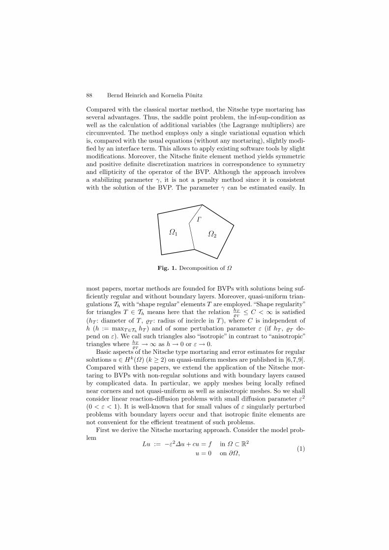
88 Bernd Heinrich and Kornelia Ponitz
Compared with the classical mortar method, the Nitsche type mortaring hasseveral advantages. Thus, the saddle point problem, the inf-sup-condition aswell as the calculation of additional variables (the Lagrange multipliers) arecircumvented. The method employs only a single variational equation whichis, compared with the usual equations (without any mortaring), slightly modi-fied by an interface term. This allows to apply existing software tools by slightmodifications. Moreover, the Nitsche finite element method yields symmetricand positive definite discretization matrices in correspondence to symmetryand ellipticity of the operator of the BVP. Although the approach involvesa stabilizing parameter γ, it is not a penalty method since it is consistentwith the solution of the BVP. The parameter γ can be estimated easily. In
Γ
Ω2Ω1
Fig. 1. Decomposition of Ω
most papers, mortar methods are founded for BVPs with solutions being suf-ficiently regular and without boundary layers. Moreover, quasi-uniform trian-gulations Th with“shape regular”elements T are employed.“Shape regularity”for triangles T ∈ Th means here that the relation hT
T≤ C < ∞ is satisfied
(hT : diameter of T , T : radius of incircle in T ), where C is independent ofh (h := maxT∈Th
hT ) and of some pertubation parameter ε (if hT , T de-pend on ε). We call such triangles also “isotropic” in contrast to “anisotropic”triangles where hT
T→∞ as h→ 0 or ε→ 0.
Basic aspects of the Nitsche type mortaring and error estimates for regularsolutions u ∈ Hk(Ω) (k ≥ 2) on quasi-uniform meshes are published in [6,7,9].Compared with these papers, we extend the application of the Nitsche mor-taring to BVPs with non-regular solutions and with boundary layers causedby complicated data. In particular, we apply meshes being locally refinednear corners and not quasi-uniform as well as anisotropic meshes. So we shallconsider linear reaction-diffusion problems with small diffusion parameter ε2
(0 < ε < 1). It is well-known that for small values of ε singularly perturbedproblems with boundary layers occur and that isotropic finite elements arenot convenient for the efficient treatment of such problems.
First we derive the Nitsche mortaring approach. Consider the model prob-lem
Lu := −ε2∆u+ cu = f in Ω ⊂ R2
u = 0 on ∂Ω,(1)
Nitsche Finite Element Method for Elliptic Problems 89
where Ω is assumed to be a polygonal domain with Lipschitz-boundary ∂Ωconsisting of straight segments. The following two cases are taken into account:
a) ε = 1 and c = 0 on Ω (the Poisson equation, corners on ∂Ω),b) 0 < ε < 1 and 0 < c0 ≤ c on Ω (singularly perturbed problem),
with some constant c0, and c ∈ L∞(Ω). Furthermore, assume f ∈ L2(Ω) atleast.
For simplicity the domain Ω is decomposed into two non-overlapping,polygonal subdomains Ω1 and Ω2 such that Ω = Ω1 ∪ Ω2 and Ω1 ∩ Ω2 = ∅hold, cf. Fig. 1. Introduce Γ := Ω1 ∩Ω2 to be the interface of Ω1 and Ω2. Inthis context, we utilize the restrictions vi :=v|Ωi
of some function v on Ωi as
well as the vectorized form v =(v1, v2
), i.e., we have vi(x) = v(x) for x ∈ Ωi
(i = 1, 2). So we shall use here the same symbol v for denoting the function von Ω as well as the vector v =
(v1, v2
), which should not lead to confusion.
Using the domain decomposition, BVP (1) is equivalent to the followingproblem. Find u =
(u1, u2
)such that
−ε2∆ui + cui = f i in Ωi, ui = 0 on ∂Ωi ∩ ∂Ω, for i = 1, 2,
∂u1
∂n1+∂u2
∂n2= 0 on Γ, u1 = u2 on Γ,
(2)
are satisfied, where ni (i = 1, 2) denotes the outward normal to ∂Ωi ∩ Γ .Define H1
0 (Ω) :=v ∈ H1(Ω) : v|∂Ω = 0
and use the variational equation of
(1). Find u ∈ H10 (Ω) such that
a(u, v) = f(v) for any v ∈ H10 (Ω), (3)
with a(u, v) := ε2∫
Ω
(∇u,∇v) dx+
∫
Ω
cuv dx, f(v) :=
∫
Ω
fv dx.
It is well-known that there is a unique solution u ∈ H 32+δ(Ω) of (3), with
some δ > 0. Moreover, we have ∆u ∈ L2(Ω) (see [15]) and, owing to the tracetheorem, ∂u
∂n ∈ L2(Γ ). If Ω is convex, the solution is regular, i.e., u ∈ H2(Ω).Nevertheless, because of small values of ε, the solution u exhibits boundarylayers, in general.
The BVP (2) can be formulated also in a weak form (see [16]). Clearly,there is weak unique solution of (2) satisfying
(u1, u2
)∈ V , with Lui ∈ L2(Ωi)
for i = 1, 2. Here, the space V is defined by V := V 1×V 2, with V i := vi : vi ∈H1(Ωi), v
i∣∣∂Ω∩∂Ωi
= 0 for ∂Ω ∩ ∂Ωi = ∅, V i := H1(Ωi) for ∂Ω ∩ ∂Ωi = ∅(i = 1, 2). The continuity of the solution u and of its normal derivative ∂ui
∂n on
Γ (n = n1 or n = n2) is to be required in the sense of H12∗ (Γ ) and H
− 12
∗ (Γ )
(the dual space of H12∗ (Γ )), respectively. For Γ like in Fig. 1 (∂Ω ∩Γ = ∅) we
define H12∗ (Γ ) as the trace space H
1200(Γ ) of H1
0 (Ω) provided with the quotient
norm, see e.g. [2,15]. In the case ∂Ω ∩Γ = ∅ we employ H12∗ (Γ ) := H
12 (Γ ). In
the following, 〈. , .〉Γ denotes the H− 1
2∗ -H
12∗ duality pairing. With this notation,
(2) implies formally
90 Bernd Heinrich and Kornelia Ponitz
2∑
i=1
(∫
Ωi
ε2(∇ui,∇vi
)dx+
∫
Ωi
cuv dx−⟨ε2∂ui
∂ni, vi
⟩
Γ
)=
2∑
i=1
∫
Ωi
f ivi dx
(4)
∀v ∈ V , or equivalently, owing to ∂u1
∂n1= α1
∂u1
∂n1−α2
∂u2
∂n2= − ∂u2
∂n2for any αi ≥ 0
(i = 1, 2) such that α1 + α2 = 1,
2∑
i=1
(∫
Ωi
ε2(∇ui,∇vi
)dx+
∫
Ωi
cuv dx
)−⟨α1ε
2 ∂u1
∂n1− α2ε
2 ∂u2
∂n2, v1 − v2
⟩
Γ
−⟨α1ε
2 ∂v1
∂n1− α2ε
2 ∂v2
∂n2, u1 − u2
⟩
Γ
+
∫
Γ
σ(u1 − u2
) (v1 − v2
)ds
=2∑
i=1
∫
Ωi
f ivi dx.
(5)
Note that the two additional terms (both equal to zero) containing u1 − u2
and introduced artificially have the following purpose. The first one ensuresthe symmetry (in u, v) of the left-hand side, the second one penalizes (afterthe discretization) the jump of the trace of the approximate solution andguarantees the stability for appropriately chosen weighting function σ > 0.The Nitsche mortar finite element method is the Galerkin discretization ofequation (5) in the sense of (8) given subsequently, using a finite elementsubspace Vh of V allowing non-matching meshes and discontinuity of the finiteelement approximation along Γ . The function σ is taken as γε2h−1(x), whereγ > 0 is a sufficiently large constant, h(x) is a mesh parameter function on Γ .
2 Non-matching mesh finite element discretization
Let T ih be a triangulation of Ωi (i = 1, 2) consisting of triangles T (T = T ).
The triangulations T 1h and T 2
h are independent of each other, in general, i.e. thenodes of T ∈ T i
h (i = 1, 2) do not match along Γ := ∂Ω1 ∩ ∂Ω2. Let h denotethe mesh parameter of the triangulation Th := T 1
h ∪ T 2h , with 0 < h ≤ h0
and sufficiently small h0. Take e.g. h := maxT∈ThhT . Admit that hT and T
may depend on the parameter ε ∈ (0, 1) (cf. (14)). Furthermore, employ F(F = F ) for denoting any side of a triangle, hF its length. Sometimes we useTF in order to indicate that F is a side of T = TF . Throughout the paper letthe following assumption on the geometrical conformity of T i
h (i = 1, 2) besatisfied. Assume that for i = 1, 2, it holds Ωi =
⋃T∈T i
hT , and two arbitrary
triangles T, T ′ ∈ T ih (T = T ′) are either disjoint or have a common vertex, or
a common side. Since anisotropic triangles (see [17]) will be applied, they arenot shape regular and, therefore, the mesh is not quasi-uniform (with respectto ε).
Consider further some triangulation Eh of the interface Γ by intervals E(E = E), i.e., Γ =
⋃E∈Eh
E, where hE denotes the diameter of E. Here, two
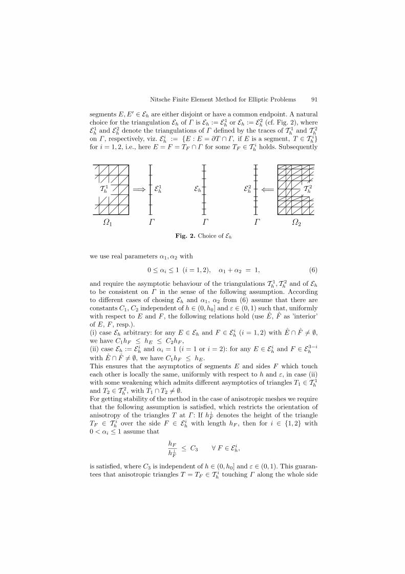
Nitsche Finite Element Method for Elliptic Problems 91
segments E,E′ ∈ Eh are either disjoint or have a common endpoint. A naturalchoice for the triangulation Eh of Γ is Eh := E1
h or Eh := E2h (cf. Fig. 2), where
E1h and E2
h denote the triangulations of Γ defined by the traces of T 1h and T 2
h
on Γ , respectively, viz. E ih := E : E = ∂T ∩ Γ, if E is a segment, T ∈ T i
hfor i = 1, 2, i.e., here E = F = TF ∩ Γ for some TF ∈ T i
h holds. Subsequently
Γ
EhE1h
ΓΩ1
T 1h =⇒
Γ
E2h T 2
h
Ω2
⇐=
Fig. 2. Choice of Eh
we use real parameters α1, α2 with
0 ≤ αi ≤ 1 (i = 1, 2), α1 + α2 = 1, (6)
and require the asymptotic behaviour of the triangulations T 1h , T 2
h and of Ehto be consistent on Γ in the sense of the following assumption. Accordingto different cases of chosing Eh and α1, α2 from (6) assume that there areconstants C1, C2 independent of h ∈ (0, h0] and ε ∈ (0, 1) such that, uniformlywith respect to E and F , the following relations hold (use E, F as ’interior’of E, F , resp.).(i) case Eh arbitrary: for any E ∈ Eh and F ∈ E i
h (i = 1, 2) with E ∩ F = ∅,we have C1hF ≤ hE ≤ C2hF ,(ii) case Eh := E i
h and αi = 1 (i = 1 or i = 2): for any E ∈ E ih and F ∈ E3−i
h
with E ∩ F = ∅, we have C1hF ≤ hE .This ensures that the asymptotics of segments E and sides F which toucheach other is locally the same, uniformly with respect to h and ε, in case (ii)with some weakening which admits different asymptotics of triangles T1 ∈ T 1
h
and T2 ∈ T 2h , with T1 ∩ T2 = ∅.
For getting stability of the method in the case of anisotropic meshes we requirethat the following assumption is satisfied, which restricts the orientation ofanisotropy of the triangles T at Γ : If h⊥F denotes the height of the triangleTF ∈ T i
h over the side F ∈ E ih with length hF , then for i ∈ 1, 2 with
0 < αi ≤ 1 assume that
hF
h⊥F≤ C3 ∀ F ∈ E i
h,
is satisfied, where C3 is independent of h ∈ (0, h0] and ε ∈ (0, 1). This guaran-tees that anisotropic triangles T = TF ∈ T i
h touching Γ along the whole side
92 Bernd Heinrich and Kornelia Ponitz
F and being “active” (for i : αi = 0) in the approximation have their “shortside” F on Γ .For i = 1, 2, introduce the finite element space V i
h of functions on Ωi by
V ih := vi
h ∈ H1(Ωi) : vih
∣∣T∈ Pk(T ) ∀ T ∈ T i
h , vih
∣∣∂Ωi∩∂Ω
= 0,
where Pk(T ) denotes the set of all polynomials on T with degree ≤ k. Thefinite element space Vh of functions vh with components vi
h on Ωi is givenby Vh := V 1
h × V 2h . In general, vh ∈ Vh is not continuous across Γ . For the
approximation of (5) on Vh let us fix a positive constant γ (to be specifiedsubsequently) and real parameters α1, α2 from (6), and introduce the formsBh(. , .) on Vh × Vh and Fh(.) on Vh as follows:
Bh(uh, vh) :=2∑
i=1
(ε2(∇ui
h,∇vih
)Ωi
+(cui
h, vih
)Ωi
)−⟨α1ε
2 ∂u1h
∂n1− α2ε
2 ∂u2h
∂n2, v1h − v2h
⟩
Γ
−⟨α1ε
2 ∂v1h
∂n1− α2ε
2 ∂v2h
∂n2, u1
h − u2h
⟩
Γ
+ ε2γ∑
E∈Eh
h−1E
(u1
h − u2h, v
1h − v2h
)E,
Fh(vh) :=
2∑
i=1
(f, vi
h
)Ωi. (7)
Here, (. , .)Λ denotes the scalar product in L2(Λ) for Λ ∈ Ωi, E, and 〈. , .〉Γis taken from (5). The weights in the fourth term of Bh are introduced in cor-respondence to σ = γε2h−1(x) at (5) and ensure the stability of the method,if γ is a sufficiently large positive constant (cf. Theorem 2 below).
According to (5), but with the discrete forms Bh and Fh from (7), theNitsche mortar finite element approximation uh of the solution u of equation(3), with respect to the space Vh, is defined by uh =
(u1
h, u2h
)∈ V 1
h ×V 2h being
the solution ofBh(uh, vh) = Fh(vh) ∀ vh ∈ Vh. (8)
In the following, we quote some important properties of the discretiza-tion (8). First we have the consistency: If u is the weak solution of (1), thenu =
(u1, u2
)satisfies Bh(u, vh) = Fh(vh) ∀ vh ∈ Vh . Then, owing to the
consistency and to (8) we obtain the Bh-orthogonality of the error u− uh onVh, i.e. Bh(u−uh, vh) = 0 ∀ vh ∈ Vh. For getting stability and convergenceof the method, we need the following theorem.
Theorem 1. For vh ∈ Vh the inequality
∑
E∈Eh
hE
∥∥∥∥α1∂v1h∂n1− α2
∂v2h∂n2
∥∥∥∥2
0,E
≤ CI
2∑
i=1
∥∥∇vih
∥∥2
0,Ωi,
holds, where CI is independent of h (h ≤ h0) and of ε (ε < 1).
Nitsche Finite Element Method for Elliptic Problems 93
The proof is given in [14]. For the ellipticity of the discrete form Bh(. , .)we introduce the following discrete energy-like norm ‖ . ‖1,h,
‖vh‖21,h =2∑
i=1
(ε2∥∥∇vi
h
∥∥2
0,Ωi+∥∥√cvi
h
∥∥2
0,Ωi
)+ ε2
∑
E∈Eh
h−1E
∥∥v1h − v2h∥∥2
0,E.
(9)For ε = 1 and c ≡ 0 this norm is also applied e.g. in [2, 6, 9, 10, 12, 13]. UsingYoung’s inequality and Theorem 1 we can prove the following theorem.
Theorem 2. If the constant γ in (7) is chosen (independently of h and ε)such that γ > CI is valid, CI from Theorem 1, then
Bh(vh,vh) ≥ µ1 ‖vh‖21,h ∀ vh ∈ Vh
holds, with a positive constant µ1 independent of h (h ≤ h0) and ε (ε < 1).
3 Numerical treatment of corner singularities
We now study the finite element approximation with non-matching meshes forthe case that the domain Ω has re-entrant corners and that the endpoints ofthe interface Γ are vertices of such corners. It is well-known that such cornersgenerate singularities enlarging the dicretization error and diminishing therate of convergence of the finite element approximation. If Ω has re-entrantcorners with angles ϕ0j : π < ϕ0j < 2π (j = 1, . . . , I), then the solution u canbe represented by
u =
I∑
j=1
ηj aj rλj
j sin(λjϕj) + w,
with a regular remainder w ∈ H2(Ω). Here, (rj , ϕj) denote the local po-lar coordinates of a point P ∈ Ω with respect to the vertex Pj ∈ ∂Ω,where 0 < rj ≤ r0j and 0 < ϕj < ϕ0j hold. Moreover, we have λj = π
ϕ0j
( 12 < λj < 1), aj is some constant, and ηj is a local cut-off function atPj . Obviously, u ∈ Hs(Ω) for some s > 3/2 is satisfied. For approaches toimprove the approximation properties and to treat corner singularities, seee.g. [15,18–21]. Since the influence region of corner singularities is a local one,it suffices to consider one corner. Here we employ piecewise linear elements(k = 1 in V i
h) and triangular meshes with appropriate local refinement at onecorner.Let (x0, y0) be the coordinates of the vertex P0 of the corner, (r, ϕ) thelocal polar coordinates with center at P0, i.e. x − x0 = r cos(ϕ + ϕr),y − y0 = r sin(ϕ + ϕr), cf. Fig. 3. Define some circular sector G aroundP0, with the radius r0 > 0 and the angle ϕ0 (here: π < ϕ0 < 2π):G :=
(x, y) ∈ Ω : 0 ≤ r ≤ r0, 0 ≤ ϕ ≤ ϕ0
, G := G \ ∂G, ∂G boundary
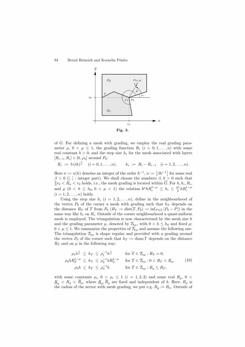
94 Bernd Heinrich and Kornelia Ponitz
y
x
Ω1
Ω2
ϕry0
x0
ϕ0
Γ
P0
ϕ
P(x,y)
r
Fig. 3.
of G. For defining a mesh with grading, we employ the real grading para-meter µ, 0 < µ ≤ 1, the grading function Ri (i = 0, 1, . . . , n) with somereal constant b > 0, and the step size hi for the mesh associated with layers[Ri−1, Ri]× [0, ϕ0] around P0:
Ri := b (ih)1µ (i = 0, 1, . . . , n), hi := Ri −Ri−1 (i = 1, 2, . . . , n).
Here n := n(h) denotes an integer of the order h−1, n :=[βh−1
]for some real
β > 0 ([ . ] : integer part). We shall choose the numbers β, b > 0 such that23r0 < Rn < r0 holds, i.e., the mesh grading is located within G. For h, hi, Ri,
and µ (0 < h ≤ h0, 0 < µ < 1) the relation bµhR1−µi ≤ hi ≤ bµ
µ hR1−µi
(i = 1, 2, . . . , n) holds.Using the step size hi (i = 1, 2, . . . , n), define in the neighbourhood of
the vertex P0 of the corner a mesh with grading such that hT depends onthe distance RT of T from P0 (RT := dist(T, P0) := infP∈T |P0 − P |) in thesame way like hi on Ri. Outside of the corner neighbourhood a quasi-uniformmesh is employed. The triangulation is now characterized by the mesh size hand the grading parameter µ, denoted by Thµ, with 0 < h ≤ h0 and fixed µ:0 < µ ≤ 1. We summarize the properties of Thµ and assume the following one:The triangulation Thµ is shape regular and provided with a grading aroundthe vertex P0 of the corner such that hT := diamT depends on the distanceRT and on µ in the following way:
ρ1h1µ ≤ hT ≤ ρ−1
1 h1µ for T ∈ Thµ : RT = 0,
ρ2hR1−µT ≤ hT ≤ ρ−1
2 hR1−µT for T ∈ Thµ : 0 < RT < Rg,
ρ3h ≤ hT ≤ ρ−13 h for T ∈ Thµ : Rg ≤ RT ,
(10)
with some constants ρi, 0 < ρi ≤ 1 (i = 1, 2, 3) and some real Rg, 0 <Rg < Rg < Rg, where Rg, Rg are fixed and independent of h. Here, Rg isthe radius of the sector with mesh grading, we put e.g. Rg := Rn. Outside of
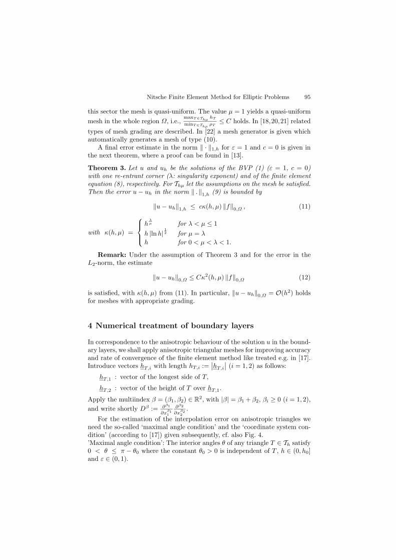
Nitsche Finite Element Method for Elliptic Problems 95
this sector the mesh is quasi-uniform. The value µ = 1 yields a quasi-uniform
mesh in the whole region Ω, i.e.,maxT∈Thµ
hT
minT∈ThµρT≤ C holds. In [18,20,21] related
types of mesh grading are described. In [22] a mesh generator is given whichautomatically generates a mesh of type (10).
A final error estimate in the norm ‖ · ‖1,h for ε = 1 and c = 0 is given inthe next theorem, where a proof can be found in [13].
Theorem 3. Let u and uh be the solutions of the BVP (1) (ε = 1, c = 0)with one re-entrant corner (λ: singularity exponent) and of the finite elementequation (8), respectively. For Thµ let the assumptions on the mesh be satisfied.Then the error u− uh in the norm ‖ . ‖1,h (9) is bounded by
‖u− uh‖1,h ≤ cκ(h, µ) ‖f‖0,Ω , (11)
with κ(h, µ) =
hλµ for λ < µ ≤ 1
h |lnh| 12 for µ = λ
h for 0 < µ < λ < 1.
Remark: Under the assumption of Theorem 3 and for the error in theL2-norm, the estimate
‖u− uh‖0,Ω ≤ Cκ2(h, µ) ‖f‖0,Ω (12)
is satisfied, with κ(h, µ) from (11). In particular, ‖u− uh‖0,Ω = O(h2) holdsfor meshes with appropriate grading.
4 Numerical treatment of boundary layers
In correspondence to the anisotropic behaviour of the solution u in the bound-ary layers, we shall apply anisotropic triangular meshes for improving accuracyand rate of convergence of the finite element method like treated e.g. in [17].Introduce vectors hT,i with length hT,i :=
∣∣hT,i
∣∣ (i = 1, 2) as follows:
hT,1 : vector of the longest side of T,
hT,2 : vector of the height of T over hT,1.
Apply the multiindex β = (β1, β2) ∈ R2, with |β| = β1 + β2, βi ≥ 0 (i = 1, 2),
and write shortly Dβ := ∂β1
∂xβ11
∂β2
∂xβ22
.
For the estimation of the interpolation error on anisotropic triangles weneed the so-called ‘maximal angle condition’ and the ‘coordinate system con-dition’ (according to [17]) given subsequently, cf. also Fig. 4.’Maximal angle condition’: The interior angles θ of any triangle T ∈ Th satisfy0 < θ ≤ π − θ0 where the constant θ0 > 0 is independent of T , h ∈ (0, h0]and ε ∈ (0, 1).
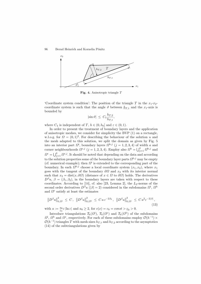
96 Bernd Heinrich and Kornelia Ponitz
ϑ
x2
x1
T
hT,1
hT,2
Fig. 4. Anisotropic triangle T
‘Coordinate system condition’: The position of the triangle T in the x1-x2-coordinate system is such that the angle ϑ between hT,1 and the x1-axis isbounded by
|sinϑ| ≤ C4hT,2
hT,1,
where C4 is independent of T , h ∈ (0, h0] and ε ∈ (0, 1).In order to present the treatment of boundary layers and the application
of anisotropic meshes, we consider for simplicity the BVP (1) on a rectangle,w.l.o.g. for Ω = (0, 1)2. For describing the behaviour of the solution u andthe mesh adapted to this solution, we split the domain as given by Fig. 5into an interior part Ωi, boundary layers Ωb,j (j = 1, 2, 3, 4) of width a and
corner neighbourhoods Ωc,j (j = 1, 2, 3, 4). Employ also Ωb =⋃4
j=1Ωb,j and
Ωc =⋃4
j=1Ωc,j . It should be noted that depending on the data and according
to the solution properties some of the boundary layer parts Ωb,j may be empty(cf. numerical example); then Ωi is extended to the corresponding part of theboundary. In each Ωb,j choose a local coordinate system (x1, x2), where x1
goes with the tangent of the boundary ∂Ω and x2 with its interior normalsuch that x2 = dist(x, ∂Ω) (distance of x ∈ Ω to ∂Ω) holds. The derivativesDβu, β = (β1, β2), in the boundary layers are taken with respect to thesecoordinates. According to [14], cf. also [23, Lemma 2], the L2-norms of thesecond order derivatives Dβu (|β| = 2) considered in the subdomains Ωi, Ωb
and Ωc satisfy at least the estimates
∥∥Dβu∥∥2
0,Ωi ≤ C ,∥∥Dβu
∥∥2
0,Ωb ≤ C a ε−2β2 ,∥∥Dβu
∥∥2
0,Ωc ≤ C a2ε−2|β| ,
(13)with a := a0
c0ε |ln ε| and a0 ≥ 2, for c(x) = c0 = const > c0 > 0.
Introduce triangulations Th(Ωi), Th(Ωc) and Th(Ωb) of the subdomainsΩi, Ωb and Ωc, respectively. For each of these subdomains employ O(h−1)×O(h−1) triangles T with mesh sizes hT,1 and hT,2 according to the asymptotics(14) of the subtriangulations given by
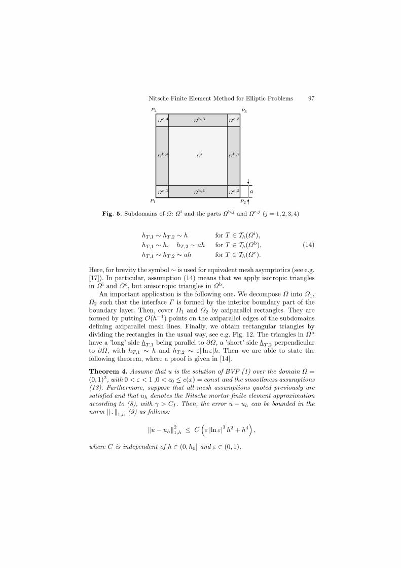
Nitsche Finite Element Method for Elliptic Problems 97
P4 P3
P1 P2
a
Ωc,4 Ωb,3 Ωc,3
Ωb,4
Ωc,1 Ωb,1 Ωc,2
Ωi Ωb,2
Fig. 5. Subdomains of Ω: Ωi and the parts Ωb,j and Ωc,j (j = 1, 2, 3, 4)
hT,1 ∼ hT,2 ∼ h for T ∈ Th(Ωi),
hT,1 ∼ h, hT,2 ∼ ah for T ∈ Th(Ωb),
hT,1 ∼ hT,2 ∼ ah for T ∈ Th(Ωc).
(14)
Here, for brevity the symbol∼ is used for equivalent mesh asymptotics (see e.g.[17]). In particular, assumption (14) means that we apply isotropic trianglesin Ωi and Ωc, but anisotropic triangles in Ωb.
An important application is the following one. We decompose Ω into Ω1,Ω2 such that the interface Γ is formed by the interior boundary part of theboundary layer. Then, cover Ω1 and Ω2 by axiparallel rectangles. They areformed by putting O(h−1) points on the axiparallel edges of the subdomainsdefining axiparallel mesh lines. Finally, we obtain rectangular triangles bydividing the rectangles in the usual way, see e.g. Fig. 12. The triangles in Ωb
have a ’long’ side hT,1 being parallel to ∂Ω, a ’short’ side hT,2 perpendicularto ∂Ω, with hT,1 ∼ h and hT,2 ∼ ε| ln ε|h. Then we are able to state thefollowing theorem, where a proof is given in [14].
Theorem 4. Assume that u is the solution of BVP (1) over the domain Ω =(0, 1)2, with 0 < ε < 1 ,0 < c0 ≤ c(x) = const and the smoothness assumptions(13). Furthermore, suppose that all mesh assumptions quoted previously aresatisfied and that uh denotes the Nitsche mortar finite element approximationaccording to (8), with γ > CI . Then, the error u − uh can be bounded in thenorm ‖ . ‖1,h (9) as follows:
‖u− uh‖21,h ≤ C(ε |ln ε|3 h2 + h4
),
where C is independent of h ∈ (0, h0] and ε ∈ (0, 1).
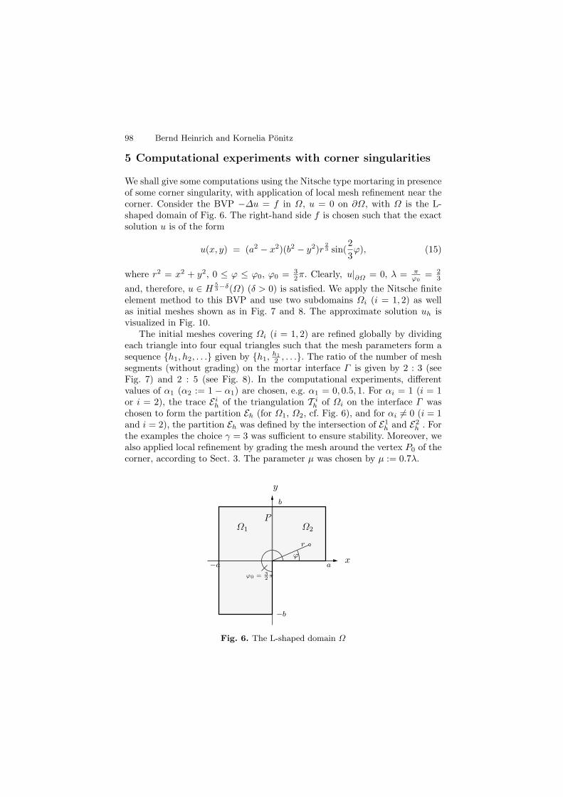
98 Bernd Heinrich and Kornelia Ponitz
5 Computational experiments with corner singularities
We shall give some computations using the Nitsche type mortaring in presenceof some corner singularity, with application of local mesh refinement near thecorner. Consider the BVP −∆u = f in Ω, u = 0 on ∂Ω, with Ω is the L-shaped domain of Fig. 6. The right-hand side f is chosen such that the exactsolution u is of the form
u(x, y) = (a2 − x2)(b2 − y2)r 23 sin(
2
3ϕ), (15)
where r2 = x2 + y2, 0 ≤ ϕ ≤ ϕ0, ϕ0 = 32π. Clearly, u|∂Ω = 0, λ = π
ϕ0= 2
3
and, therefore, u ∈ H 53−δ(Ω) (δ > 0) is satisfied. We apply the Nitsche finite
element method to this BVP and use two subdomains Ωi (i = 1, 2) as wellas initial meshes shown as in Fig. 7 and 8. The approximate solution uh isvisualized in Fig. 10.
The initial meshes covering Ωi (i = 1, 2) are refined globally by dividingeach triangle into four equal triangles such that the mesh parameters form asequence h1, h2, . . . given by h1,
h1
2 , . . .. The ratio of the number of meshsegments (without grading) on the mortar interface Γ is given by 2 : 3 (seeFig. 7) and 2 : 5 (see Fig. 8). In the computational experiments, differentvalues of α1 (α2 := 1 − α1) are chosen, e.g. α1 = 0, 0.5, 1. For αi = 1 (i = 1or i = 2), the trace E i
h of the triangulation T ih of Ωi on the interface Γ was
chosen to form the partition Eh (for Ω1, Ω2, cf. Fig. 6), and for αi = 0 (i = 1and i = 2), the partition Eh was defined by the intersection of E1
h and E2h . For
the examples the choice γ = 3 was sufficient to ensure stability. Moreover, wealso applied local refinement by grading the mesh around the vertex P0 of thecorner, according to Sect. 3. The parameter µ was chosen by µ := 0.7λ.
ϕ
−a
b
a
−b
r
Ω1 Ω2
y
x
Γ
ϕ0 = 32
π
Fig. 6. The L-shaped domain Ω
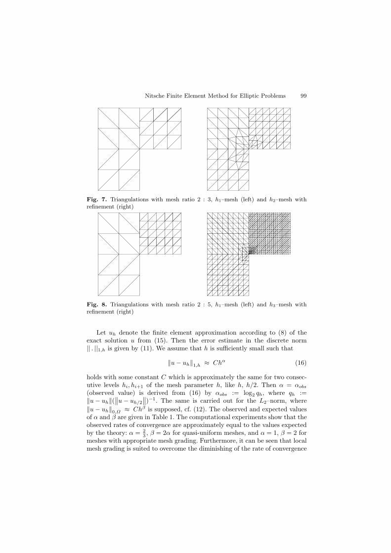
Nitsche Finite Element Method for Elliptic Problems 99
Fig. 7. Triangulations with mesh ratio 2 : 3, h1–mesh (left) and h2–mesh withrefinement (right)
Fig. 8. Triangulations with mesh ratio 2 : 5, h1–mesh (left) and h3–mesh withrefinement (right)
Let uh denote the finite element approximation according to (8) of theexact solution u from (15). Then the error estimate in the discrete norm|| . ||1,h is given by (11). We assume that h is sufficiently small such that
‖u− uh‖1,h ≈ Chα (16)
holds with some constant C which is approximately the same for two consec-utive levels hi, hi+1 of the mesh parameter h, like h, h/2. Then α = αobs
(observed value) is derived from (16) by αobs := log2 qh, where qh :=‖u− uh‖(
∥∥u− uh/2
∥∥)−1. The same is carried out for the L2–norm, where
‖u− uh‖0,Ω ≈ Chβ is supposed, cf. (12). The observed and expected valuesof α and β are given in Table 1. The computational experiments show that theobserved rates of convergence are approximately equal to the values expectedby the theory: α = 2
3 , β = 2α for quasi-uniform meshes, and α = 1, β = 2 formeshes with appropriate mesh grading. Furthermore, it can be seen that localmesh grading is suited to overcome the diminishing of the rate of convergence
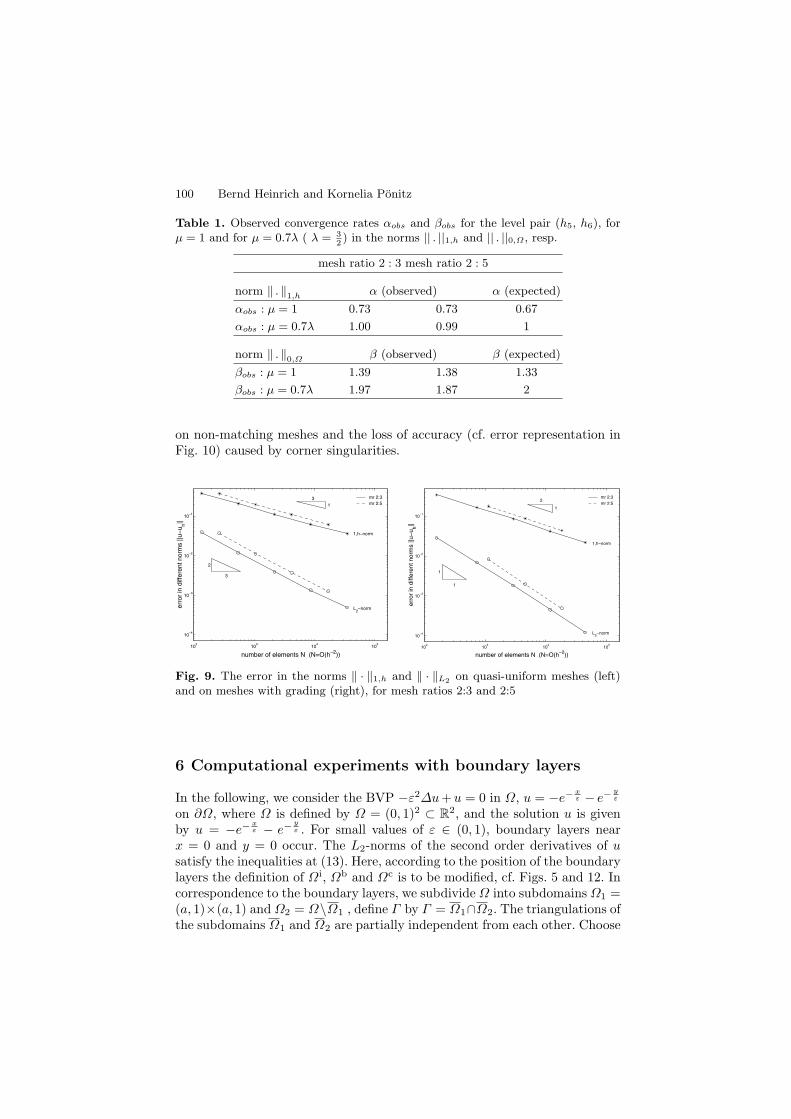
100 Bernd Heinrich and Kornelia Ponitz
Table 1. Observed convergence rates αobs and βobs for the level pair (h5, h6), forµ = 1 and for µ = 0.7λ ( λ = 3
2) in the norms || . ||1,h and || . ||0,Ω , resp.
mesh ratio 2 : 3 mesh ratio 2 : 5
norm ‖ . ‖1,h α (observed) α (expected)
αobs : µ = 1 0.73 0.73 0.67
αobs : µ = 0.7λ 1.00 0.99 1
norm ‖ . ‖0,Ω β (observed) β (expected)
βobs : µ = 1 1.39 1.38 1.33
βobs : µ = 0.7λ 1.97 1.87 2
on non-matching meshes and the loss of accuracy (cf. error representation inFig. 10) caused by corner singularities.
102
103
104
105
10−4
10−3
10−2
10−1
number of elements N (N=O(h−2))
err
or
in d
iffe
ren
t n
orm
s ||u
−u
h||
mr 2:3
mr 2:5
1,h−norm
L2−norm
2
3
3
1
102
103
104
105
10−4
10−3
10−2
10−1
number of elements N (N=O(h−2))
err
or
in d
iffe
ren
t n
orm
s ||u
−u
h||
mr 2:3
mr 2:5
1,h−norm
L2−norm
1
1
2
1
Fig. 9. The error in the norms ‖ · ‖1,h and ‖ · ‖L2 on quasi-uniform meshes (left)and on meshes with grading (right), for mesh ratios 2:3 and 2:5
6 Computational experiments with boundary layers
In the following, we consider the BVP −ε2∆u+u = 0 in Ω, u = −e− xε − e− y
ε
on ∂Ω, where Ω is defined by Ω = (0, 1)2 ⊂ R2, and the solution u is given
by u = −e− xε − e− y
ε . For small values of ε ∈ (0, 1), boundary layers nearx = 0 and y = 0 occur. The L2-norms of the second order derivatives of usatisfy the inequalities at (13). Here, according to the position of the boundarylayers the definition of Ωi, Ωb and Ωc is to be modified, cf. Figs. 5 and 12. Incorrespondence to the boundary layers, we subdivide Ω into subdomains Ω1 =(a, 1)×(a, 1) and Ω2 = Ω\Ω1 , define Γ by Γ = Ω1∩Ω2. The triangulations ofthe subdomains Ω1 and Ω2 are partially independent from each other. Choose
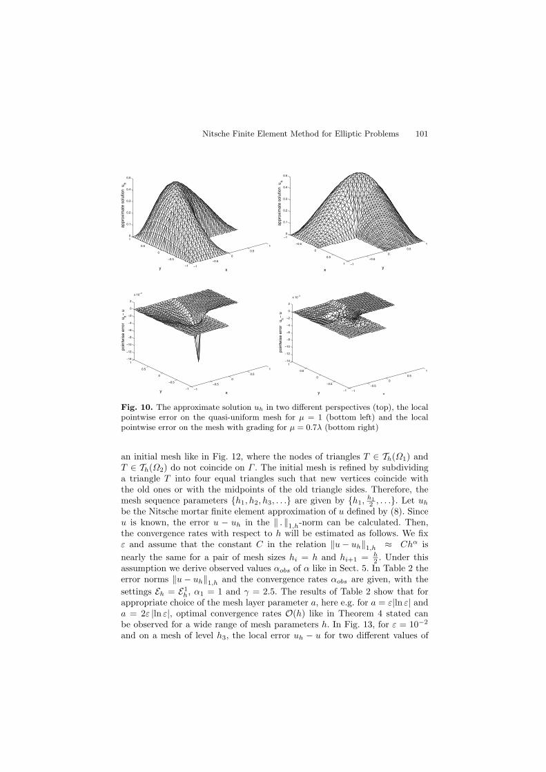
Nitsche Finite Element Method for Elliptic Problems 101
−1
−0.5
0
0.5
1
−1
−0.5
0
0.5
10
0.1
0.2
0.3
0.4
0.5
xy
ap
pro
xim
ate
so
lutio
n
uh
−1
−0.5
0
0.5
1 −1
−0.5
0
0.5
1
0
0.1
0.2
0.3
0.4
0.5
yx
ap
pro
xim
ate
so
lutio
n
uh
−1
−0.5
0
0.5
1
−1
−0.5
0
0.5
1−14
−12
−10
−8
−6
−4
−2
0
2
x 10−3
xy
po
intw
ise
err
or
u
h−
u
−1
−0.5
0
0.5
1
−1
−0.5
0
0.5
1−14
−12
−10
−8
−6
−4
−2
0
2
x 10−3
xy
poin
twis
e e
rror
u
h−
u
Fig. 10. The approximate solution uh in two different perspectives (top), the localpointwise error on the quasi-uniform mesh for µ = 1 (bottom left) and the localpointwise error on the mesh with grading for µ = 0.7λ (bottom right)
an initial mesh like in Fig. 12, where the nodes of triangles T ∈ Th(Ω1) andT ∈ Th(Ω2) do not coincide on Γ . The initial mesh is refined by subdividinga triangle T into four equal triangles such that new vertices coincide withthe old ones or with the midpoints of the old triangle sides. Therefore, themesh sequence parameters h1, h2, h3, . . . are given by h1,
h1
2 , . . .. Let uh
be the Nitsche mortar finite element approximation of u defined by (8). Sinceu is known, the error u − uh in the ‖ . ‖1,h-norm can be calculated. Then,the convergence rates with respect to h will be estimated as follows. We fixε and assume that the constant C in the relation ‖u− uh‖1,h ≈ Chα is
nearly the same for a pair of mesh sizes hi = h and hi+1 = h2 . Under this
assumption we derive observed values αobs of α like in Sect. 5. In Table 2 theerror norms ‖u− uh‖1,h and the convergence rates αobs are given, with the
settings Eh = E1h, α1 = 1 and γ = 2.5. The results of Table 2 show that for
appropriate choice of the mesh layer parameter a, here e.g. for a = ε|ln ε| anda = 2ε |ln ε|, optimal convergence rates O(h) like in Theorem 4 stated canbe observed for a wide range of mesh parameters h. In Fig. 13, for ε = 10−2
and on a mesh of level h3, the local error uh − u for two different values of
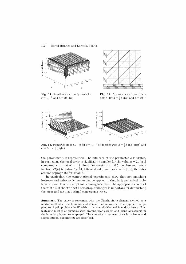
102 Bernd Heinrich and Kornelia Ponitz
00.2
0.40.6
0.81
0
0.5
1−2
−1.5
−1
−0.5
0
xy
exa
ctso
lutio
nu
a
Fig. 11. Solution u on the h3-mesh forε = 10−2 and a = 2ε |ln ε|
Fig. 12. h1-mesh with layer thick-ness a, for a = 1
2ε |ln ε| and ε = 10−1
0
0.5
1 00.2
0.40.6
0.81
−0.04
0
0.04
0.08
0.12
yx
po
intw
ise
err
or
u h−
u
0
0.5
1 00.2
0.40.6
0.81
−0.04
0
0.04
0.08
0.12
yx
po
intw
ise
err
or
u h−
u
Fig. 13. Pointwise error uh −u for ε = 10−2 on meshes with a = 12ε |ln ε| (left) and
a = 2ε |ln ε| (right)
the parameter a is represented. The influence of the parameter a is visible,in particular, the local error is significantly smaller for the value a = 2ε |ln ε|compared with that of a = 1
2ε |ln ε|. For constant a = 0.5 the observed rate isfar from O(h) (cf. also Fig. 14, left-hand side) and, for a = 1
2ε |ln ε|, the ratesare not appropriate for small h.
In particular, the computational experiments show that non-matchingisotropic and anisotropic meshes can be applied to singularly perturbed prob-lems without loss of the optimal convergence rate. The appropriate choice ofthe width a of the strip with anisotropic triangles is important for diminishingthe error and getting optimal convergence rates.
Summary. The paper is concerned with the Nitsche finite element method as amortar method in the framework of domain decomposition. The approach is ap-plied to elliptic problems in 2D with corner singularities and boundary layers. Non-matching meshes of triangles with grading near corners and being anisotropic inthe boundary layers are employed. The numerical treatment of such problems andcomputational experiments are described.
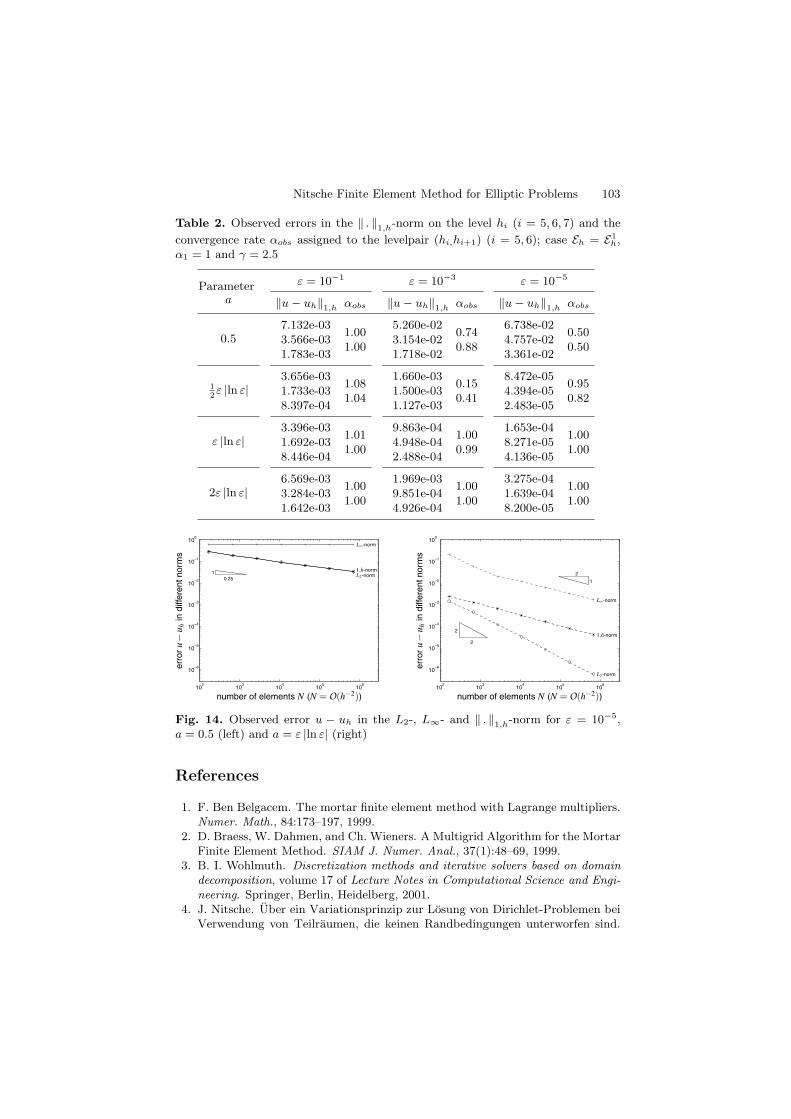
Nitsche Finite Element Method for Elliptic Problems 103
Table 2. Observed errors in the ‖ . ‖1,h-norm on the level hi (i = 5, 6, 7) and the
convergence rate αobs assigned to the levelpair (hi,hi+1) (i = 5, 6); case Eh = E1h,
α1 = 1 and γ = 2.5
Parameter ε = 10−1 ε = 10−3 ε = 10−5
a ‖u − uh‖1,h αobs ‖u − uh‖1,h αobs ‖u − uh‖1,h αobs
0.57.132e-033.566e-031.783e-03
1.001.00
5.260e-023.154e-021.718e-02
0.740.88
6.738e-024.757e-023.361e-02
0.500.50
12ε |ln ε|
3.656e-031.733e-038.397e-04
1.081.04
1.660e-031.500e-031.127e-03
0.150.41
8.472e-054.394e-052.483e-05
0.950.82
ε |ln ε|3.396e-031.692e-038.446e-04
1.011.00
9.863e-044.948e-042.488e-04
1.000.99
1.653e-048.271e-054.136e-05
1.001.00
2ε |ln ε|6.569e-033.284e-031.642e-03
1.001.00
1.969e-039.851e-044.926e-04
1.001.00
3.275e-041.639e-048.200e-05
1.001.00
102
103
104
105
106
10−6
10−5
10−4
10−3
10−2
10−1
100
10.25
number of elements N (N = O(h−2))
err
or
u−
u hin
diffe
rentnorm
s
L∞-norm
1,h-normL2-norm
102
103
104
105
106
10−6
10−5
10−4
10−3
10−2
10−1
100
2
2
2
1
number of elements N (N = O(h−2))
err
or
u−
u hin
diffe
rentnorm
s
L∞-norm
1,h-norm
L2-norm
Fig. 14. Observed error u − uh in the L2-, L∞- and ‖ . ‖1,h-norm for ε = 10−5,a = 0.5 (left) and a = ε |ln ε| (right)
References
1. F. Ben Belgacem. The mortar finite element method with Lagrange multipliers.Numer. Math., 84:173–197, 1999.
2. D. Braess, W. Dahmen, and Ch. Wieners. A Multigrid Algorithm for the MortarFinite Element Method. SIAM J. Numer. Anal., 37(1):48–69, 1999.
3. B. I. Wohlmuth. Discretization methods and iterative solvers based on domaindecomposition, volume 17 of Lecture Notes in Computational Science and Engi-neering. Springer, Berlin, Heidelberg, 2001.
4. J. Nitsche. Uber ein Variationsprinzip zur Losung von Dirichlet-Problemen beiVerwendung von Teilraumen, die keinen Randbedingungen unterworfen sind.
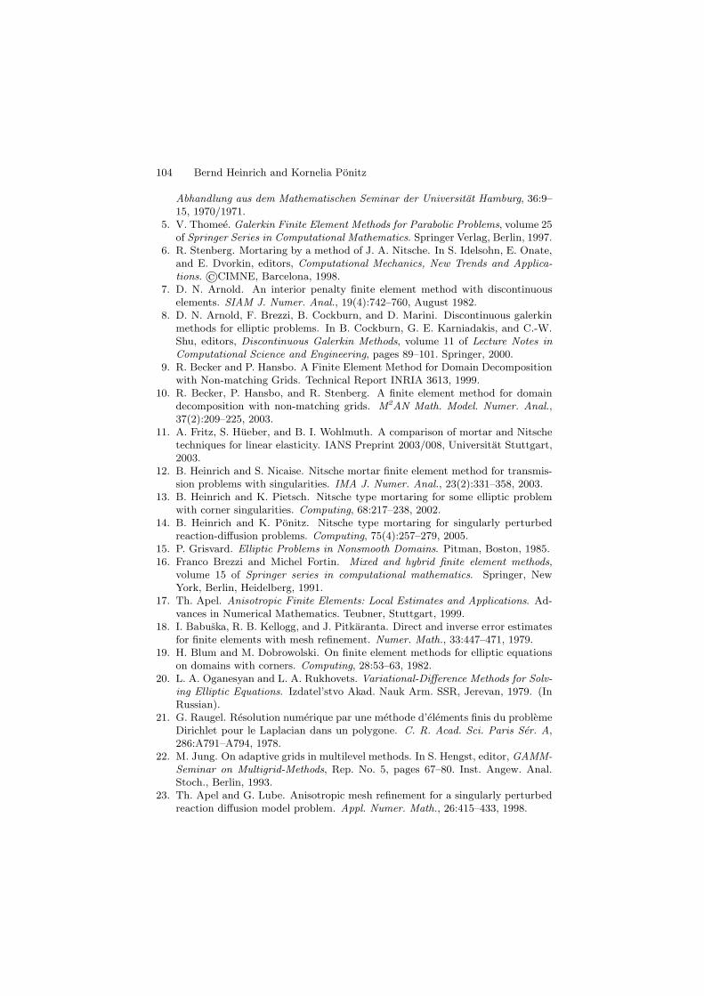
104 Bernd Heinrich and Kornelia Ponitz
Abhandlung aus dem Mathematischen Seminar der Universitat Hamburg, 36:9–15, 1970/1971.
5. V. Thomee. Galerkin Finite Element Methods for Parabolic Problems, volume 25of Springer Series in Computational Mathematics. Springer Verlag, Berlin, 1997.
6. R. Stenberg. Mortaring by a method of J. A. Nitsche. In S. Idelsohn, E. Onate,and E. Dvorkin, editors, Computational Mechanics, New Trends and Applica-tions. ©CIMNE, Barcelona, 1998.
7. D. N. Arnold. An interior penalty finite element method with discontinuouselements. SIAM J. Numer. Anal., 19(4):742–760, August 1982.
8. D. N. Arnold, F. Brezzi, B. Cockburn, and D. Marini. Discontinuous galerkinmethods for elliptic problems. In B. Cockburn, G. E. Karniadakis, and C.-W.Shu, editors, Discontinuous Galerkin Methods, volume 11 of Lecture Notes inComputational Science and Engineering, pages 89–101. Springer, 2000.
9. R. Becker and P. Hansbo. A Finite Element Method for Domain Decompositionwith Non-matching Grids. Technical Report INRIA 3613, 1999.
10. R. Becker, P. Hansbo, and R. Stenberg. A finite element method for domaindecomposition with non-matching grids. M2AN Math. Model. Numer. Anal.,37(2):209–225, 2003.
11. A. Fritz, S. Hueber, and B. I. Wohlmuth. A comparison of mortar and Nitschetechniques for linear elasticity. IANS Preprint 2003/008, Universitat Stuttgart,2003.
12. B. Heinrich and S. Nicaise. Nitsche mortar finite element method for transmis-sion problems with singularities. IMA J. Numer. Anal., 23(2):331–358, 2003.
13. B. Heinrich and K. Pietsch. Nitsche type mortaring for some elliptic problemwith corner singularities. Computing, 68:217–238, 2002.
14. B. Heinrich and K. Ponitz. Nitsche type mortaring for singularly perturbedreaction-diffusion problems. Computing, 75(4):257–279, 2005.
15. P. Grisvard. Elliptic Problems in Nonsmooth Domains. Pitman, Boston, 1985.16. Franco Brezzi and Michel Fortin. Mixed and hybrid finite element methods,
volume 15 of Springer series in computational mathematics. Springer, NewYork, Berlin, Heidelberg, 1991.
17. Th. Apel. Anisotropic Finite Elements: Local Estimates and Applications. Ad-vances in Numerical Mathematics. Teubner, Stuttgart, 1999.
18. I. Babuska, R. B. Kellogg, and J. Pitkaranta. Direct and inverse error estimatesfor finite elements with mesh refinement. Numer. Math., 33:447–471, 1979.
19. H. Blum and M. Dobrowolski. On finite element methods for elliptic equationson domains with corners. Computing, 28:53–63, 1982.
20. L. A. Oganesyan and L. A. Rukhovets. Variational-Difference Methods for Solv-ing Elliptic Equations. Izdatel’stvo Akad. Nauk Arm. SSR, Jerevan, 1979. (InRussian).
21. G. Raugel. Resolution numerique par une methode d’elements finis du problemeDirichlet pour le Laplacian dans un polygone. C. R. Acad. Sci. Paris Ser. A,286:A791–A794, 1978.
22. M. Jung. On adaptive grids in multilevel methods. In S. Hengst, editor, GAMM-Seminar on Multigrid-Methods, Rep. No. 5, pages 67–80. Inst. Angew. Anal.Stoch., Berlin, 1993.
23. Th. Apel and G. Lube. Anisotropic mesh refinement for a singularly perturbedreaction diffusion model problem. Appl. Numer. Math., 26:415–433, 1998.
Hierarchical Adaptive FEM at FiniteElastoplastic Deformations
Reiner Kreißig, Anke Bucher, and Uwe-Jens Gorke
Technische Universitat Chemnitz, Institut fur Mechanik09107 Chemnitz, [email protected]
1 Introduction
The simulation of non-linear problems of continuum mechanics was a crucialpoint within the framework of the subproject “Efficient parallel algorithmsfor the simulation of the deformation behaviour of components of inelasticmaterials”. Nonlinearity appears with the occurence of finite deformations aswell as with special material behaviour as e.g. elastoplasticity.
To solve such kind of problems by means of a Finite Element simulation forreliable predictions of the response of components and structures to mechani-cal loading, the insertion of suitable material models into FE codes is a basicrequirement. Additionally, their efficient numerical implementation plays alsoan important role.
Likewise, a realistic numerical simulation essentially depends on appro-priate FE meshes. According to the motto “as fine as necessary, as coarseas possible”, several techniques of mesh adaptation have been developed inthe last decades. These days the feature of adaptivity is a high-performanceattribute for FE codes.
We want to present the results of our research within the framework ofthe subproject D1 concerning the efficient treatment of non-linear problemsof continuum mechanics:
• The theoretical development and numerical realization of appropriate ma-terial laws for elastoplasticity and,
• the implementation of hierarchical mesh adaptation in case of non-linearmaterial behaviour.
All contrived theoretical descriptions and numerical algorithms had beenimplemented and tested with the in-house code SPC-PM2AdNl which wasdeveloped at the Chemnitz University of Technology within the context ofour collaborative research centre 393.
106 Reiner Kreißig et al.
2 Material model for finite elastoplastic deformations
This section deals with the formulation and efficient numerical implementationof a material model decsribing finite elastoplasticity.
2.1 Theoretical foundation and thermodynamical consistency
The presented approach for the establishment of elastoplastic material mod-els considering finite deformations is based on the multiplicative split of thedeformation gradient F = F eF p into an elastic part F e and a plastic partF p. The plastic part of the deformation gradient realizes the mapping of thedeformed body from the reference to the plastic intermediate configuration,the elastic part the remaining mapping from the plastic intermediate to thecurrent configuration (see Fig. 1). It has to be mentioned that the plasticintermediate configuration is an incompatible one.
In the literature different approaches to model plastic anisotropy are pre-sented:
• Hill developed a quadratic yield condition for the special case of plasticorthotropy [16].
• General plastic anisotropy can be treated in a phenomenological mannerintroducing special (tensorial) internal variables describing the hardeningbehaviour [2, 6, 15,26,30].
• Another possibility to describe general plastic anisotropy consists in theapplication of microstructural approaches [3, 13,25,27,32].
• Several authors propose phenomenological models based on so-called sub-structure concepts [12, 18, 24, 28]. This procedure is based on the consid-eration of microstructural characteristics of the material (substructure)using macroscopic constitutive approaches (definition of special internalvariables). The continuum and the underlying substructure are supposedto have different characteristics of orientation.
The substructure approach has been developed particularely by Mandel [24]and Dafalias [12]. The last mentioned distinguished between the kinematics ofthe continuum and the kinematics of the substructure in a phenomenologicalmanner introducing a special deformation gradient F S = F eβ related to thesubstructure, where the tensor β is supposed to be an orthogonal one. Justas Mandel he defined special objective time derivatives connected with thesubstructure using its spin ωD.
The spin of the continuum is defined as
w =1
2
F eF e−1 − F e−T
F eT
+ (1)
1
2
F e
F pF p−1F e−1 − F e−T F p−T
F pTF eT
= weD + w
pD. (2)
Hierarchical Adaptive FEM at Finite Elastoplastic Deformations 107
with
F p = F p − ωDF p,
F e = F e + F eωD and ωD = ββ−1. (3)
The crucial point of Dafalias’ approach consists in the assumption of an evo-lutional equation for the plastic spin w
pD, which represents the difference be-
tween the spin of the continuum and the substructure spin:
wpD = w − ωD with ωD = ˙ββ
−1and β = Reβ , (4)
where Re represents the rotation tensor of the elastic part of the deforma-tion gradient. Dafalias did not give a thermodynamical explanation for thesuggested evolutional equation for w
pD.
In the following we define a substructure configuration apart from the con-figurations describing the deformation of a continuum. A mapping tensor H
is supposed to map tensorial variables from the reference into this substruc-ture configuration. Accordingly, the tensor combination F H−1 serves themapping from the substructure configuration into the current configuration.The substructure configuration is assumed to be an incompatible intermediateconfiguration characterizing a special constitutively motivated decompositionof the deformation gradient. It differs from the plastic intermediate configu-ration only by a rotation characterized by the tensor β (see Fig. 1). In thefollowing, variables related to the substructure configuration are denoted bycapital letters with a hat.
In the framework of the presented phenomenological material model, theevolution of stresses and strains is considered with respect to the continuum.The internal variables describing the plastic anisotropy are related to thesubstructure. Therefore, the substructure configuration is connected with anewly established objective time derivative. This Lie-type derivative is definedin case of a contravariant tensor as follows:
a = F H−1
(H F −1aF −T
︸ ︷︷ ︸A
HT)·
H−T F T
= F H−1(H AHT + H AHT + H AHT
)H−T F T
= F H−1 ˙AH−T F T . (5)
It should be mentioned that the definition of this objective time derivative isclosely connected with the supposition of the existence of a material derivativein the substructure configuration.
If the mapping tensor is supposed to be defined as
H = βT F p, (6)
we getF H−1 = F eβ = F S (7)
and following the plastic spin at the reference configuration can be written
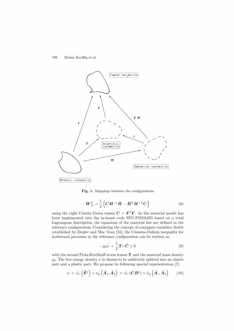
108 Reiner Kreißig et al.
Fig. 1. Mappings between the configurations
WpD =
1
2
CH−1H − HT H−T C
(8)
using the right Cauchy-Green tensor C = F TF . As the material model hasbeen implemented into the in-house code SPC-PM2AdNl based on a totalLagrangean description, the equations of the material law are defined in thereference configuration. Considering the concept of conjugate variables, firstlyestablished by Ziegler and Mac Vean [35], the Clausius-Duhem inequality forisothermal processes in the reference configuration can be written as
−0ψ +1
2T ·· C ≥ 0 (9)
with the second Piola-Kirchhoff stress tensor T and the material mass density0. The free energy density ψ is chosen to be additively splitted into an elasticpart and a plastic part. We propose its following special representation [7]:
ψ = ψe
(Ee
)+ ψp
(A1, A2
)= ψe (CBp) + ψp
(A1, A2
)(10)
Hierarchical Adaptive FEM at Finite Elastoplastic Deformations 109
with Bp = Cp−1 = F p−1F p−T (11)
introducing a covariant symmetric second-order tensorial internal variable A1
and a covariant skew-symmetric one A2, both defined in the substructureconfiguration. Based on relation (9) we get the following inequality consideringthe time derivative of equation (10):
−o
∂ψe
∂ (CBp)·· (BpC )
·+∂ψp
∂A1
·· A1˙ − ∂ψp
∂A2
·· A2˙
+1
2T ·· C ≥ 0 . (12)
In the case of pure elastic material behaviour no dissipation does appear,and a hyperelastic material law can be defined easily from (12):
T = 2 o∂ψe
∂ (CBp)Bp = 2
∂ψe
∂C. (13)
Describing the material behaviour of metals we propose a modified compress-ible Neo-Hookean model for the elastic part of the free energy density [7] withmaterial parameters which can be estimated based on the Young’s modulusand the Poisson’s ratio.
Considering the assumptions
α = 0∂ψp
∂A1
, T p = −0∂ψp
∂A2
(14)
for the backstress tensor α work-conjugated to A1 and for a stress-like ten-sor T p work-conjugated to A2 in the remaining part of the Clausius-Duheminequality (12) after the elimination of the hyperelastic relation, we get theplastic dissipation inequality formulated in the reference configuration
Dp = −α ··
A1 − T p ··
A2 −1
2CT Cp·· Bp ≥ 0 (15)
with
α = H−1αH−T ,
A1 = HT A1˙
H ,
T p = H−1T pH−T ,
A2 = HT A2˙
H .
(16)
Considering the postulate that the plastic dissipation has to achieve amaximum under the constraint of satisfying an appropriate yield condition
F (T ,α,T p) ≤ 0 (17)
(see e. g. [31]), a corresponding constrained optimization problem based onthe method of Lagrangean multipliers can be defined as follows:
M = Dp (T , α, T p) − λG (T , α, T p, y) → stat (18)
where λ represents the plastic multiplier and y a slip variable with
110 Reiner Kreißig et al.
G = F (T , α, T p) + y2. (19)
The analysis of the necessary conditions (also known as Kuhn-Tucker condi-tions) for the objective function M to be a stationary point results in theassociated flow rule
Bp = −2λB∂F
∂TBp with B = C−1 (20)
and the evolutional equations for the internal variables
A1 = −λ∂F∂α,
A2 = λ∂F
∂T p . (21)
The tensors α and A1 respectively T p and A2 are variables assumed to beconnected by the following free energy density relation defined in the sub-structure configuration with its metric tensor G
ψp =1
2c1GA1··GA1 −
1
2c2GA2··GA2. (22)
This approach with (14) and a subsequent mapping into the reference config-uration leads to
α = c1X A1X , T p = −c2X A2X (23)
α = c1X
A1X ,
T p = −c2X
A2X (24)
withX = H−1GH−T . (25)
Due to the dependency of the yield condition on the equivalent stressTF which on its part represents a function of the plastic arc length Ep
v itis necessary to consider an evolutional equation for Ep
v . Following the usualrepresentation the rate of the plastic arc length is given by
Epv =
√2
3BpEp ·· BpEp with Ep =
1
2(Cp −G) . (26)
The tensor G represents the metric of the reference configuration. Finallywe get the following system of differential and algebraic equations (DAE)as a material model describing anisotropic finite elastoplastic deformationsconsidering an underlying substructure:
Hierarchical Adaptive FEM at Finite Elastoplastic Deformations 111
T + λD4
··∂ F
∂ T− 1
2D4
·· C + λ
(T∂F
∂TB + B
∂F
∂TT
)= 0 (27)
α + Q1 (T ,α ,T p, λ) = 0 (28)
T p + Q2 (T ,α ,T p, λ) = 0 (29)
Epv + Q3 (T ,α ,T p, λ) = 0 (30)
F (T ,α ,T p) = 0 (31)
with D4
= 4∂2ψe
∂C ∂C(32)
Q1 = c1X
(λ∂F
∂α
)X + H−1H α + αHT H−T (33)
Q2 = c2X
(λ∂F
∂T p
)X + H−1H T p + T pHT H−T (34)
Q3 = −λ√
2
3B∂ F
∂ T·· B
∂ F
∂ T. (35)
The DAE (27)-(31) represents the initial value problem which has to besolved within the equilibrium iterations at each Gauss point.
2.2 Numerical solution of the initial value problem
Generally, initial boundary value problems of finite elastoplasticity can not besolved analytically. Therefore numerical solution methods have to be applied.
Within the context of numerical solution strategies there exist differentkinds of proceeding. In our case we have chosen a method implying the si-multaneous integration of the complete system of differential and algebraicequations. This procedure has some advantages we want to elaborate afterhaving given its numerical implementation in the following.
Using the implizit single step discretization scheme
yn+1 = yn + (α fn+1 + (1− α) fn) ∆ t (36)
for the solution of the differential equation
dy
dt= y = f(t, y) (37)
with the time increment ∆ t = tn+1 − tn and the weighting factor α ∈ [0, 1]we get the following time discretization of equations (27)-(31):
112 Reiner Kreißig et al.
T n+1 − T n −[α
1
2D4
n+1··Cn+1 + (1− α)1
2D4
n··Cn
]∆t
+
[αλn+1 D
4n+1··
∂ F
∂ T
∣∣∣∣n+1
+ (1− α)λn D4
n··∂ F
∂ T
∣∣∣∣n
]∆t
+αλn+1
[T n+1
∂ F
∂ T
∣∣∣∣n+1
Bn+1 + Bn+1∂ F
∂ T
∣∣∣∣n+1
T n+1
]∆t
+ (1− α)λn
[T n
∂ F
∂ T
∣∣∣∣n
Bn + Bn∂ F
∂ T
∣∣∣∣n
T n
]∆t = 0 (38)
αn+1 −αn +[αQ1n+1
+ (1− α)Q1n
]∆t = 0 (39)
T pn+1 − T p
n +[αQ2n+1
+ (1− α)Q2n
]∆t = 0 (40)
Epvn+1
− Epvn
+[αQ3n+1
+ (1− α)Q3n
]∆t = 0 (41)
F (T n+1,αn+1,Tpn+1) = 0 (42)
To eliminate the material time derivative Cn+1, which can not be calculatedfrom other available values, relation (36) is applied once again:
Cn+1 =1
α∆t
[∆Cn+1 − (1− α) Cn∆t
](43)
with
∆Cn+1 = Cn+1 −Cn (α = 1 for the load step n = 0 ) (44)
and equation (38) becomes:
T n+1− T n+
[αλn+1 D
4n+1··
∂ F
∂ T
∣∣∣∣n+1
+(1− α)λn D4
n··∂ F
∂ T
∣∣∣∣n
]∆t
− 1
2D4
n+1··∆Cn+1 −1
2(1− α)
(D4
n −D4
n+1
)··Cn ∆t
+αλn+1
[T n+1
∂ F
∂ T
∣∣∣∣n+1
Bn+1 + Bn+1∂ F
∂ T
∣∣∣∣n+1
T n+1
]∆t
+ (1− α)λn
[T n
∂ F
∂ T
∣∣∣∣n
Bn + Bn∂ F
∂ T
∣∣∣∣n
T n
]∆t = 0 . (45)
Relations (45), (39)–(42) represent a non-linear system of algebraic equationswith respect to T n+1, αn+1, T
pn+1, E
pv n+1 and λn+1. In the following a vector
of variablesz = (T ,α ,T p, Ep
v , λ)T
(46)
Hierarchical Adaptive FEM at Finite Elastoplastic Deformations 113
is introduced. The left-hand side of the system of equations (45),(39)-(42) canbe written using an operator G
G = G(zn,zn+1,∆Cn+1, Cn
). (47)
As we can consider the vectors zn and Cn as known and therefore fixedquantities, the vector zn+1
zn+1 =(T n+1,αn+1,T
pn+1, E
pvn+1
, λn+1
)T
(48)
represents the solution of the non-linear system of algebraic equations
Gn+1 = G (zn+1) = 0 (49)
with respect to the load step [tn, tn+1]. For the calculation of zn+1 from (49)the Newton’s method is applied. This kind of proceeding leads to a linearsystem of algebraic equations
(∇
zin+1
G
)∆z i+1
n+1 = − Gin+1, (50)
for the iterative determination of the increments of the solution vector z
∆z i+1n+1 = z i+1
n+1 − z in+1. (51)
This kind of proceeding to solve the initial value problem has an impor-tant advantage: The consistent material tangent dT /dE necessary for thegeneration of the element stiffnes matrices can be calculated very easily. Fromthe implicit differentiation of equations (45),(39)-(42), cp. (47) and (49), withrespect to the strain tensor E follows
2dG
dCn+1=
dG
dEn+1=
∂ G
∂En+1+
(∇zn+1 G
) dzn+1
dEn+1= 0 . (52)
Because of the Jacobi matrix in equation (52) is always known the consistentmaterial tangent can be calculated immediately without any further efforts:
(∇zn+1 G
)
dTdE|n+1
dαdE|n+1
dT p
dE|n+1
dEpv
dE|n+1
dλdE|n+1
=
D4
n+1 + M4
n+1
04
04
0
0
(53)
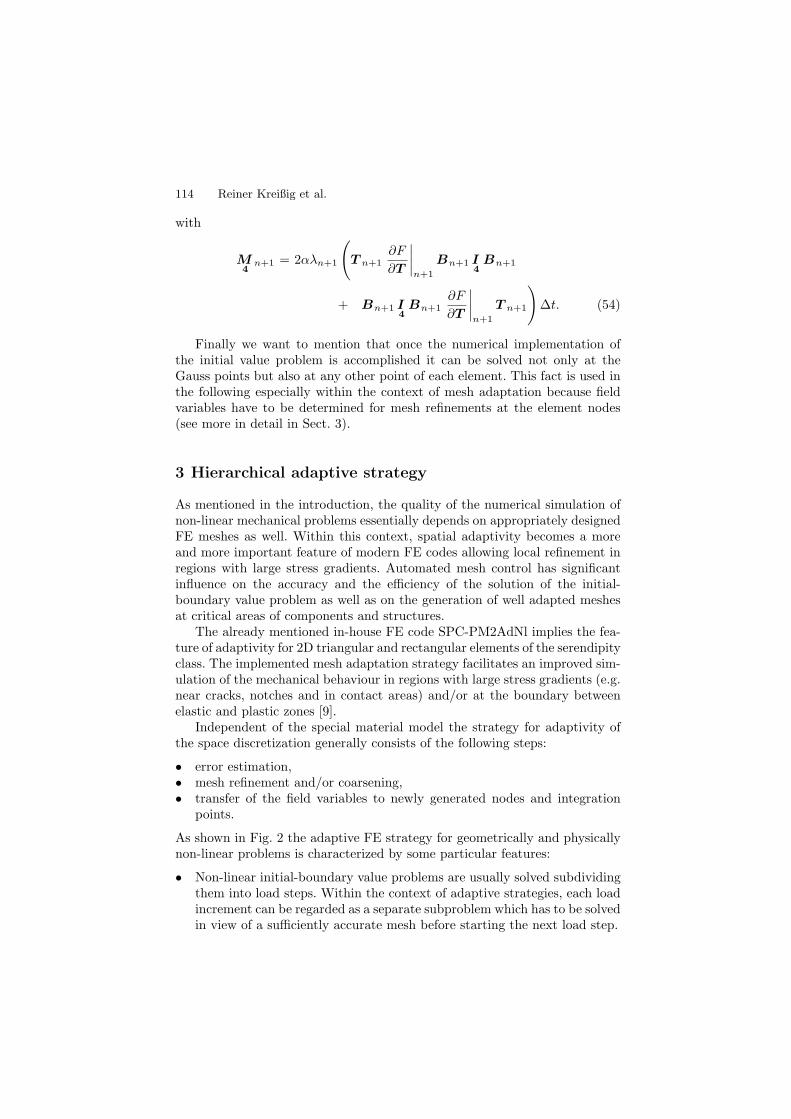
114 Reiner Kreißig et al.
with
M4
n+1 = 2αλn+1
(T n+1
∂F
∂T
∣∣∣∣n+1
Bn+1 I4
Bn+1
+ Bn+1 I4
Bn+1∂F
∂T
∣∣∣∣n+1
T n+1
)∆t. (54)
Finally we want to mention that once the numerical implementation ofthe initial value problem is accomplished it can be solved not only at theGauss points but also at any other point of each element. This fact is used inthe following especially within the context of mesh adaptation because fieldvariables have to be determined for mesh refinements at the element nodes(see more in detail in Sect. 3).
3 Hierarchical adaptive strategy
As mentioned in the introduction, the quality of the numerical simulation ofnon-linear mechanical problems essentially depends on appropriately designedFE meshes as well. Within this context, spatial adaptivity becomes a moreand more important feature of modern FE codes allowing local refinement inregions with large stress gradients. Automated mesh control has significantinfluence on the accuracy and the efficiency of the solution of the initial-boundary value problem as well as on the generation of well adapted meshesat critical areas of components and structures.
The already mentioned in-house FE code SPC-PM2AdNl implies the fea-ture of adaptivity for 2D triangular and rectangular elements of the serendipityclass. The implemented mesh adaptation strategy facilitates an improved sim-ulation of the mechanical behaviour in regions with large stress gradients (e.g.near cracks, notches and in contact areas) and/or at the boundary betweenelastic and plastic zones [9].
Independent of the special material model the strategy for adaptivity ofthe space discretization generally consists of the following steps:
• error estimation,• mesh refinement and/or coarsening,• transfer of the field variables to newly generated nodes and integration
points.
As shown in Fig. 2 the adaptive FE strategy for geometrically and physicallynon-linear problems is characterized by some particular features:
• Non-linear initial-boundary value problems are usually solved subdividingthem into load steps. Within the context of adaptive strategies, each loadincrement can be regarded as a separate subproblem which has to be solvedin view of a sufficiently accurate mesh before starting the next load step.
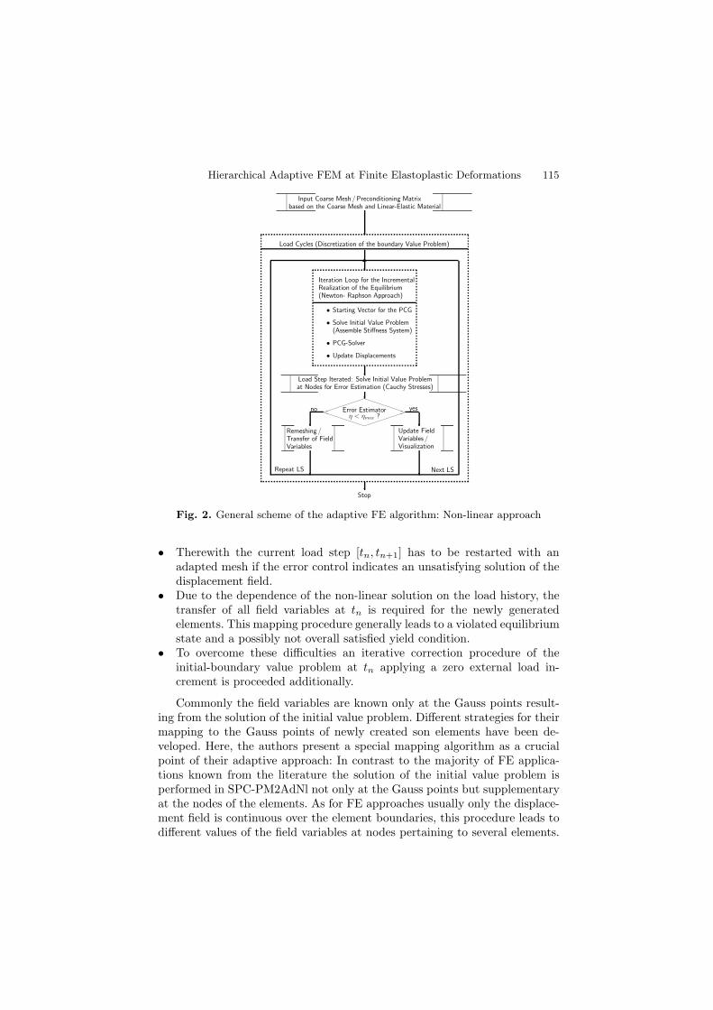
Hierarchical Adaptive FEM at Finite Elastoplastic Deformations 115
Input Coarse Mesh / Preconditioning Matrixbased on the Coarse Mesh and Linear-Elastic Material
Load Cycles (Discretization of the boundary Value Problem)
Iteration Loop for the IncrementalRealization of the Equilibrium(Newton- Raphson Approach)
• Starting Vector for the PCG
• Solve Initial Value Problem(Assemble Stiffness System)
• PCG-Solver
• Update Displacements
Load Step Iterated: Solve Initial Value Problemat Nodes for Error Estimation (Cauchy Stresses)
Error Estimatorη < ηmax ?
Update FieldVariables /Visualization
Next LS
Remeshing /Transfer of FieldVariables
Repeat LS
Stop
no yes
•
Fig. 2. General scheme of the adaptive FE algorithm: Non-linear approach
• Therewith the current load step [tn, tn+1] has to be restarted with anadapted mesh if the error control indicates an unsatisfying solution of thedisplacement field.
• Due to the dependence of the non-linear solution on the load history, thetransfer of all field variables at tn is required for the newly generatedelements. This mapping procedure generally leads to a violated equilibriumstate and a possibly not overall satisfied yield condition.
• To overcome these difficulties an iterative correction procedure of theinitial-boundary value problem at tn applying a zero external load in-crement is proceeded additionally.
Commonly the field variables are known only at the Gauss points result-ing from the solution of the initial value problem. Different strategies for theirmapping to the Gauss points of newly created son elements have been de-veloped. Here, the authors present a special mapping algorithm as a crucialpoint of their adaptive approach: In contrast to the majority of FE applica-tions known from the literature the solution of the initial value problem isperformed in SPC-PM2AdNl not only at the Gauss points but supplementaryat the nodes of the elements. As for FE approaches usually only the displace-ment field is continuous over the element boundaries, this procedure leads todifferent values of the field variables at nodes pertaining to several elements.
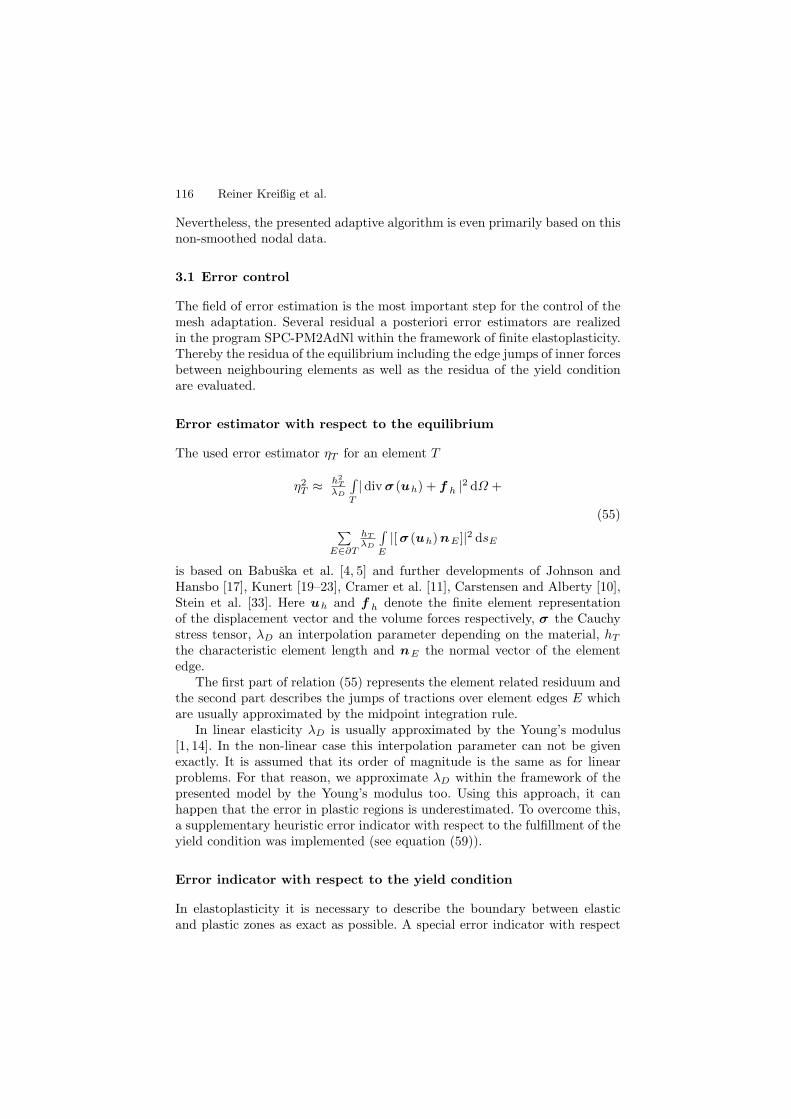
116 Reiner Kreißig et al.
Nevertheless, the presented adaptive algorithm is even primarily based on thisnon-smoothed nodal data.
3.1 Error control
The field of error estimation is the most important step for the control of themesh adaptation. Several residual a posteriori error estimators are realizedin the program SPC-PM2AdNl within the framework of finite elastoplasticity.Thereby the residua of the equilibrium including the edge jumps of inner forcesbetween neighbouring elements as well as the residua of the yield conditionare evaluated.
Error estimator with respect to the equilibrium
The used error estimator ηT for an element T
η2T ≈h2
T
λD
∫T
|div σ (uh) + f h |2 dΩ +
∑E∈∂T
hT
λD
∫E
|[σ (uh)nE ]|2 dsE
(55)
is based on Babuska et al. [4, 5] and further developments of Johnson andHansbo [17], Kunert [19–23], Cramer et al. [11], Carstensen and Alberty [10],Stein et al. [33]. Here uh and f h denote the finite element representationof the displacement vector and the volume forces respectively, σ the Cauchystress tensor, λD an interpolation parameter depending on the material, hT
the characteristic element length and nE the normal vector of the elementedge.
The first part of relation (55) represents the element related residuum andthe second part describes the jumps of tractions over element edges E whichare usually approximated by the midpoint integration rule.
In linear elasticity λD is usually approximated by the Young’s modulus[1, 14]. In the non-linear case this interpolation parameter can not be givenexactly. It is assumed that its order of magnitude is the same as for linearproblems. For that reason, we approximate λD within the framework of thepresented model by the Young’s modulus too. Using this approach, it canhappen that the error in plastic regions is underestimated. To overcome this,a supplementary heuristic error indicator with respect to the fulfillment of theyield condition was implemented (see equation (59)).
Error indicator with respect to the yield condition
In elastoplasticity it is necessary to describe the boundary between elasticand plastic zones as exact as possible. A special error indicator with respect
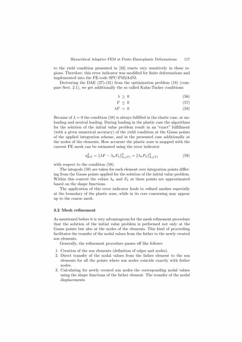
Hierarchical Adaptive FEM at Finite Elastoplastic Deformations 117
to the yield condition presented in [33] reacts very sensitively in these re-gions. Therefore, this error indicator was modified for finite deformations andimplemented into the FE-code SPC-PM2AdNl.
Derivating the DAE (27)-(31) from the optimization problem (18) (com-pare Sect. 2.1), we get additionally the so called Kuhn-Tucker conditions:
λ ≥ 0 (56)
F ≤ 0 (57)
λF = 0 (58)
Because of λ = 0 the condition (58) is always fulfilled in the elastic case, at un-loading and neutral loading. During loading in the plastic case the algorithmsfor the solution of the initial value problem result in an “exact” fulfillment(with a given numerical accuracy) of the yield condition at the Gauss pointsof the applied integration scheme, and in the presented case additionally atthe nodes of the elements. How accurate the plastic zone is mapped with thecurrent FE mesh can be estimated using the error indicator
η2KT = ‖λF − λhFh‖2L2(T ) = ‖λhFh‖2L2(T ) (59)
with respect to the condition (58).The integrals (59) are taken for each element over integration points differ-
ing from the Gauss points applied for the solution of the initial value problem.Within this context the values λh and Fh at these points are approximatedbased on the shape functions.
The application of this error indicator leads to refined meshes especiallyat the boundary of the plastic zone, while in its core coarsening may appearup to the coarse mesh.
3.2 Mesh refinement
As mentioned before it is very advantageous for the mesh refinement procedurethat the solution of the initial value problem is performed not only at theGauss points but also at the nodes of the elements. This kind of proceedingfacilitates the transfer of the nodal values from the father to the newly createdson elements.
Generally, the refinement procedure passes off like follows:
1. Creation of the son elements (definition of edges and nodes).2. Direct transfer of the nodal values from the father element to the son
elements for all the points where son nodes coincide exactly with fathernodes.
3. Calculating for newly created son nodes the corresponding nodal valuesusing the shape functions of the father element. The transfer of the nodaldisplacements
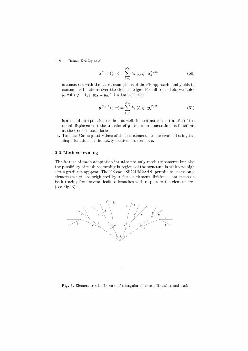
118 Reiner Kreißig et al.
uSonj (ξ, η) =
Nel∑
k=1
hk (ξ, η) uFathk (60)
is consistent with the basic assumptions of the FE approach, and yields tocontinuous functions over the element edges. For all other field variablesyi with y = (y1, y2, ..., yn)
Tthe transfer rule
ySonj (ξ, η) =
Nel∑
k=1
hk (ξ, η) yFathk (61)
is a useful interpolation method as well. In contrast to the transfer of thenodal displacements the transfer of y results in noncontinuous functionsat the element boundaries.
4. The new Gauss point values of the son elements are determined using theshape functions of the newly created son elements.
3.3 Mesh coarsening
The feature of mesh adaptation includes not only mesh refinements but alsothe possibility of mesh coarsening in regions of the structure in which no highstress gradients apppear. The FE code SPC-PM2AdNl permits to coarse onlyelements which are originated by a former element division. That means aback tracing from several leafs to branches with respect to the element tree(see Fig. 3).
1
12 3 4
15
26 3 7
4
8
1
9
10 11
6 12
3 13
7 144
15
8
16
5 2
Fig. 3. Element tree in the case of triangular elements: Branches and leafs
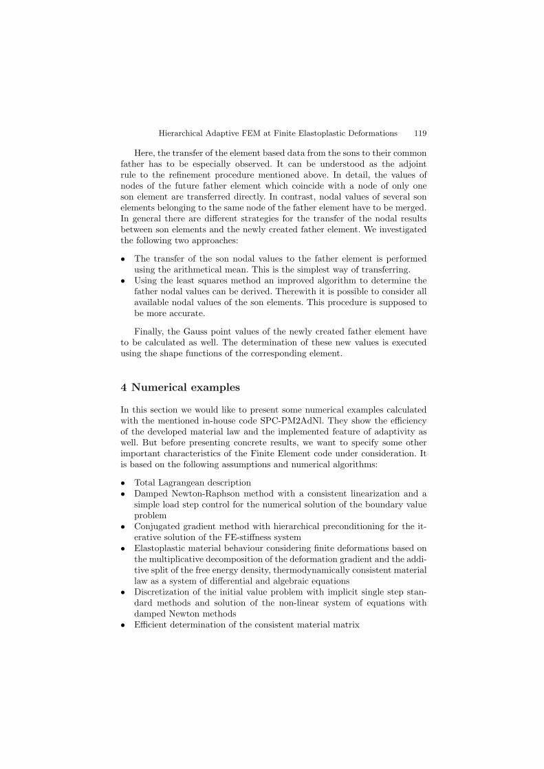
Hierarchical Adaptive FEM at Finite Elastoplastic Deformations 119
Here, the transfer of the element based data from the sons to their commonfather has to be especially observed. It can be understood as the adjointrule to the refinement procedure mentioned above. In detail, the values ofnodes of the future father element which coincide with a node of only oneson element are transferred directly. In contrast, nodal values of several sonelements belonging to the same node of the father element have to be merged.In general there are different strategies for the transfer of the nodal resultsbetween son elements and the newly created father element. We investigatedthe following two approaches:
• The transfer of the son nodal values to the father element is performedusing the arithmetical mean. This is the simplest way of transferring.
• Using the least squares method an improved algorithm to determine thefather nodal values can be derived. Therewith it is possible to consider allavailable nodal values of the son elements. This procedure is supposed tobe more accurate.
Finally, the Gauss point values of the newly created father element haveto be calculated as well. The determination of these new values is executedusing the shape functions of the corresponding element.
4 Numerical examples
In this section we would like to present some numerical examples calculatedwith the mentioned in-house code SPC-PM2AdNl. They show the efficiencyof the developed material law and the implemented feature of adaptivity aswell. But before presenting concrete results, we want to specify some otherimportant characteristics of the Finite Element code under consideration. Itis based on the following assumptions and numerical algorithms:
• Total Lagrangean description• Damped Newton-Raphson method with a consistent linearization and a
simple load step control for the numerical solution of the boundary valueproblem
• Conjugated gradient method with hierarchical preconditioning for the it-erative solution of the FE-stiffness system
• Elastoplastic material behaviour considering finite deformations based onthe multiplicative decomposition of the deformation gradient and the addi-tive split of the free energy density, thermodynamically consistent materiallaw as a system of differential and algebraic equations
• Discretization of the initial value problem with implicit single step stan-dard methods and solution of the non-linear system of equations withdamped Newton methods
• Efficient determination of the consistent material matrix
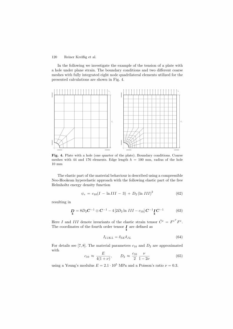
120 Reiner Kreißig et al.
In the following we investigate the example of the tension of a plate witha hole under plane strain. The boundary conditions and two different coarsemeshes with fully integrated eight node quadrilateral elements utilized for thepresented calculations are shown in Fig. 4.
Fig. 4. Plate with a hole (one quarter of the plate). Boundary conditions. Coarsemeshes with 44 and 176 elements. Edge length h = 100 mm, radius of the hole10 mm
The elastic part of the material behaviour is described using a compressibleNeo-Hookean hyperelastic approach with the following elastic part of the freeHelmholtz energy density function
ψe = c10(I − ln III − 3) + D2 (ln III)2
(62)
resulting in
D4
= 8D2C−1 ⊗C−1 − 4 [2D2 ln III − c10] C−1I
4C−1 (63)
Here I and III denote invariants of the elastic strain tensor Ce = F eT
F e.The coordinates of the fourth order tensor I
4are defined as
IIJKL = δIKδJL (64)
For details see [7, 8]. The material parameters c10 and D2 are approximatedwith
c10 ≈E
4(1 + ν), D2 ≈
c102
ν
1− 2ν(65)
using a Young’s modulus E = 2.1 · 105 MPa and a Poisson’s ratio ν = 0.3.
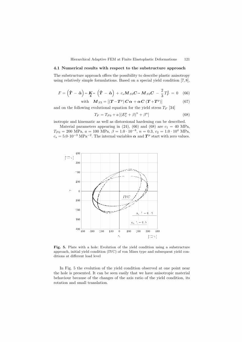
Hierarchical Adaptive FEM at Finite Elastoplastic Deformations 121
4.1 Numerical results with respect to the substructure approach
The substructure approach offers the possibility to describe plastic anisotropyusing relatively simple formulations. Based on a special yield condition [7, 8],
F =(T − α
)·· K
4··(T − α
)+ csM S3C ·· M S3C − 2
3T 2
F = 0 (66)
with M S3 = [(T −T p) Cα + αC (T +T p)] (67)
and on the following evolutional equation for the yield stress TF [34]
TF = TF0 + a [(Epv + β)
n+ βn] (68)
isotropic and kinematic as well as distorsional hardening can be described.Material parameters appearing in (24), (66) and (68) are c1 = 40 MPa,
TF0 = 200 MPa, a = 100 MPa, β = 1.0 · 10−8, n = 0.3, c2 = 1.0 · 104 MPa,cs = 5.0·10−3 MPa−2. The internal variables α and T p start with zero values.
IYC
Fig. 5. Plate with a hole: Evolution of the yield condition using a substructureapproach, initial yield condition (IYC) of von Mises type and subsequent yield con-ditions at different load level
In Fig. 5 the evolution of the yield condition observed at one point nearthe hole is presented. It can be seen easily that we have anisotropic materialbehaviour because of the changes of the axis ratio of the yield condition, itsrotation and small translation.
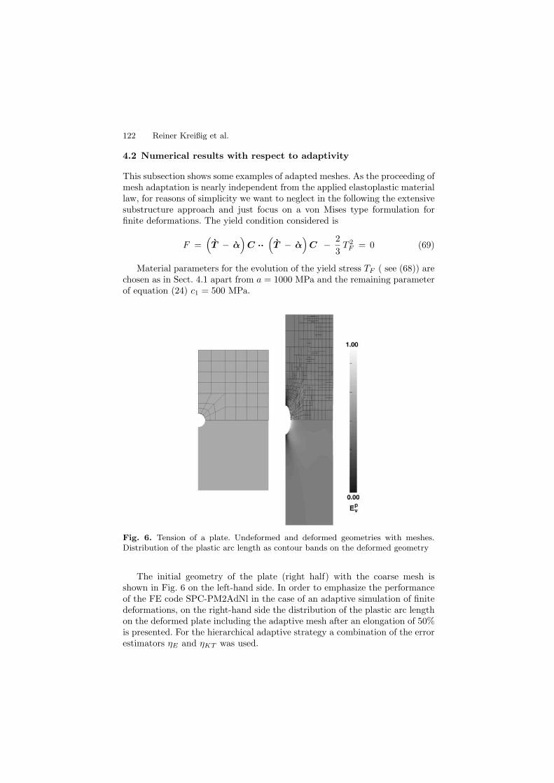
122 Reiner Kreißig et al.
4.2 Numerical results with respect to adaptivity
This subsection shows some examples of adapted meshes. As the proceeding ofmesh adaptation is nearly independent from the applied elastoplastic materiallaw, for reasons of simplicity we want to neglect in the following the extensivesubstructure approach and just focus on a von Mises type formulation forfinite deformations. The yield condition considered is
F =(T − α
)C ··
(T − α
)C − 2
3T 2
F = 0 (69)
Material parameters for the evolution of the yield stress TF ( see (68)) arechosen as in Sect. 4.1 apart from a = 1000 MPa and the remaining parameterof equation (24) c1 = 500 MPa.
Fig. 6. Tension of a plate. Undeformed and deformed geometries with meshes.Distribution of the plastic arc length as contour bands on the deformed geometry
The initial geometry of the plate (right half) with the coarse mesh isshown in Fig. 6 on the left-hand side. In order to emphasize the performanceof the FE code SPC-PM2AdNl in the case of an adaptive simulation of finitedeformations, on the right-hand side the distribution of the plastic arc lengthon the deformed plate including the adaptive mesh after an elongation of 50%is presented. For the hierarchical adaptive strategy a combination of the errorestimators ηE and ηKT was used.
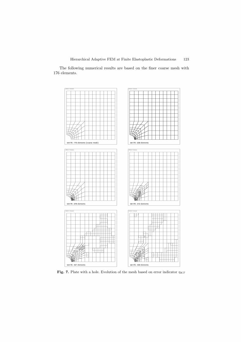
Hierarchical Adaptive FEM at Finite Elastoplastic Deformations 123
The following numerical results are based on the finer coarse mesh with176 elements.
bln176 - 176 Elemente (Grobgitter)
SFB 393 - TU Chemnitz
elements (coarse mesh) bln176 - 208 Elemente
SFB 393 - TU Chemnitz
elements
bln176 - 278 Elemente
SFB 393 - TU Chemnitz
elements bln176 - 312 Elemente
SFB 393 - TU Chemnitz
elements
bln176 - 407 Elemente
SFB 393 - TU Chemnitz
elements bln176 - 409 Elemente
SFB 393 - TU Chemnitz
elements
Fig. 7. Plate with a hole. Evolution of the mesh based on error indicator ηKT
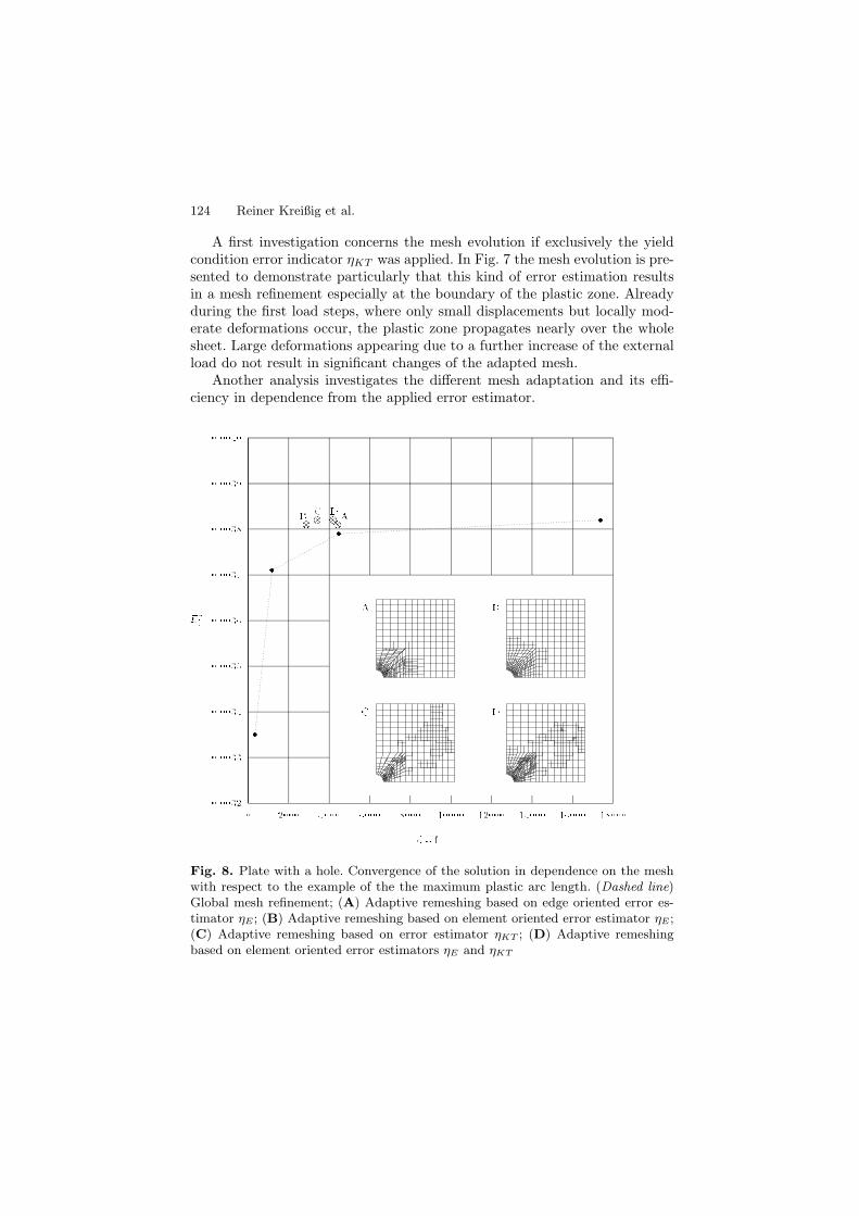
124 Reiner Kreißig et al.
A first investigation concerns the mesh evolution if exclusively the yieldcondition error indicator ηKT was applied. In Fig. 7 the mesh evolution is pre-sented to demonstrate particularly that this kind of error estimation resultsin a mesh refinement especially at the boundary of the plastic zone. Alreadyduring the first load steps, where only small displacements but locally mod-erate deformations occur, the plastic zone propagates nearly over the wholesheet. Large deformations appearing due to a further increase of the externalload do not result in significant changes of the adapted mesh.
Another analysis investigates the different mesh adaptation and its effi-ciency in dependence from the applied error estimator.
Fig. 8. Plate with a hole. Convergence of the solution in dependence on the meshwith respect to the example of the the maximum plastic arc length. (Dashed line)Global mesh refinement; (A) Adaptive remeshing based on edge oriented error es-timator ηE ; (B) Adaptive remeshing based on element oriented error estimator ηE ;(C) Adaptive remeshing based on error estimator ηKT ; (D) Adaptive remeshingbased on element oriented error estimators ηE and ηKT
Hierarchical Adaptive FEM at Finite Elastoplastic Deformations 125
It can be seen that error estimation with respect to the equilibrium (ηE) yieldsto an element refinement at locations with high stress gradients (compare casesA and B in Fig. 8). In comparison, the yield condition error indicator ηKT leadsto new elements especially at the boundary of the plastic zone. Generally itcan be observed that for all kinds of error estimation the presented hierarchicaladaptive strategy provides the asymptotic values of the field variables alreadyat much lower element numbers compared with a global remeshing approach.
5 Outlook
Within the framework of the simulation of non-linear problems in continuummechanics we focused our activities especially on the development of suitablematerial laws for finite elastoplasticity as well as on the implementation ofadaptive hierarchical remeshing strategies.
Future developments will concern the development of a 3D code versionas well as the extension to mixed finite FE approaches. The objective is toenlarge the application field of our developments to more technical problemsand also to the field of biomechanics.
References
1. T. Apel, R. Mucke and J.R. Whiteman. An adaptive finite element techniquewith a-priori mesh grading. Report 9, BICOM Institute of Computational Math-ematics, 1993.
2. N. Aravas. Finite strain anisotropic plasticity: Constitutive equations and com-putational issues. Advances in finite deformation problems in materials process-ing and structures. ASME 125 : 25–32, 1991.
3. R. Asaro. Crystal plasticity. J Appl Mech 50 : 921–934, 1983.4. I. Babuska, W.C. Rheinboldt. A-posteriori error estimates for the finite element
method. Int J Numerical Meth Eng 12 : 1597–1615, 1978.5. I. Babuska, A. Miller. A-posteriori error estimates and adaptive techniques for
the finite element method. Technical report, Institute for Physical Science andTechnology, University of Maryland, 1981.
6. D. Besdo. Zur anisotropen Verfestigung anfangs isotroper starrplastischer Me-dien. ZAMM 51 : T97–T98, 1971.
7. A. Bucher. Deformationsgesetze fur große elastisch-plastische Verzerrungenunter Berucksichtigung einer Substruktur. PhD thesis, TU Chemnitz, 2001.
8. A. Bucher, U.-J. Gorke and R. Kreißig. A material model for finite elasto-plasticdeformations considering a substructure. Int. J. Plasticity 20 : 619–642, 2004.
9. A. Bucher, A. Meyer, U.-J. Gorke, R. Kreißig. A contribution to error estima-tion and mapping algorithms for a hierarchical adaptive FE-strategy in finiteelastoplasticity. Comput. Mech. 36 : 182–195, 2005.
10. C. Carstensen, J. Alberty. Averaging techniques for reliable a posteriori FE-error control in elastoplasticity with hardening. Comput. Method. Appl. Mech.Engrg. 192 : 1435–1450, 2003.
126 Reiner Kreißig et al.
11. H. Cramer, M. Rudolph, G. Steinl, W. Wunderlich. A hierarchical adaptivefinite element strategy for elastic-plastic problems. Comput. Struct. 73 : 61–72,1999.
12. Y.F. Dafalias. A missing link in the macroscopic constitutive formulation oflarge plastic deformations. In: Plasticity today, (Sawczuk, A., Bianchi, G. eds.),from the International Symposium on Recent Trends and Results in Plasticity,Elsevier, Udine, p.135, 1983.
13. Y.F. Dafalias. On the microscopic origin of the plastic spin. Acta Mech. 82 : 31–48, 1990.
14. J.P. Gago, D. Kelly, O.C. Zienkiewicz and I. Babuska. A-posteriori error analysisand adaptive processes in the finite element method. Part I: Error analysis. PartII: Adaptive processes. Int. J. Num. Meth. Engng., 19/83 : 1593–1656, 1983.
15. P. Haupt. On the concept of an intermediate configuration and its applicationto a representation of viscoelastic-plastic material behavior. Int. J. Plasticity,1 : 303–316.
16. R. Hill. A theory of yielding and plastic flow of anisotropic metals. Proc. Roy.Soc. of London A 193, 281–297, 1948.
17. C. Johnson, P. Hansbo. Adaptive finite element methods in computationalmechanics. Comput. Methods Appl. Mech. Engrg. 101 : 143–181, 1992.
18. J. Kratochvil. Finite strain theory of cristalline elastic-plastic materials. ActaMech. 16 : 127–142, 1973.
19. G. Kunert. Error estimation for anisotropic tetrahedral and triangular finiteelement meshes. Preprint SFB393/97-16, TU Chemnitz, 1997.
20. G. Kunert. An a posteriori residual error estimator for the finite element methodon anisotropic tetrahedral meshes. Numer. Math., 86(3) : 471–490, 2000.
21. G. Kunert. A local problem error estimator for anisotropic tetrahedral finiteelement meshes. SIAM J. Numer. Anal. 39 : 668–689, 2001.
22. G. Kunert. A posteriori l2 error estimation on anisotropic tetrahedral finiteelement meshes. IMA J. Numer. Anal. 21 : 503–523, 2001.
23. G. Kunert and R. Verfurth. Edge residuals dominate a posteriori error esti-mates for linear finite element methods on anisotropic triangular and tetrahedralmeshes. Numer. Math., 86(2):283–303, 2000.
24. J. Mandel. Plasticite classique et viscoplasticite. CISM Courses and LecturesNo.97, Springer-Verlag, Berlin, 1971.
25. C. Miehe, J. Schotte, J. Schroder. Computational micro-macro transitions andoverall moduli in the analysis of polycristals at large strains. Comp. Mat. Sci.16 : 372–382, 1999.
26. J. Ning, E.C. Aifantis. On anisotropic finite deformation plasticity, Part I. Atwo-back stress model. Acta Mech. 106 : 55–72, 1994.
27. J. Ning, E.C. Aifantis. Anisotropic yield and plastic flow of polycristalline solids.Int. J. Plasticity 12 : 1221–1240, 1996.
28. E.T. Onat. Representation of inelastic behaviour in the presence of anisotropyand of finite deformations. In: Recent advances in creep and fracture of engi-neering materials and structures, Pineridge Press, Swansea, 1982.
29. S.S. Rao. Engineering Optimization. John Wiley and Sons, New York, 1996.30. C. Sansour. On anisotropy at the actual configuration and the adequate formula-
tion of a free energy function. IUTAM Symposium on Anisotropy, Inhomogenityand Nonlinearity in Solid Mechanics, 43–50, 1995.
Hierarchical Adaptive FEM at Finite Elastoplastic Deformations 127
31. J.C. Simo. A framework for finite strain elastoplasticity based on maximumplastic dissipation and the multiplicative decomposition: Part I. Continuum for-mulation. Comput. Methods Appl. Mech. Engrg. 66 : 199–219, 1988.
32. E. Steck. Zur Berucksichtigung von Vorgangen im Mikrobereich metallischerWerkstoffe bei der Entwicklung von Stoffmodellen. ZAMM 75 : 331–341, 1995.
33. E. Stein (Ed.). Error-controlled Adaptive Finite Elements in Solid Mechanics.Wiley, Chichester, 2003.
34. V. Ulbricht, H. Rohle. Berechnung von Rotationsschalen bei nichtlinearem De-formationsverhalten, PhD thesis, TU Dresden, 1975.
35. H. Ziegler, D. Mac Vean. On the notion of an elastic solid. In: B. Broberg, J.Hult and F. Niordson, eds., Recent Progress in Appl. Mech. The Folke OdquistVolume, Eds. B. Broberg, J. Hult, F. Niordson, Almquist & Wiksell, Stockholm,561–572, 1965.

Wavelet Matrix Compression for BoundaryIntegral Equations
Helmut Harbrecht1, Ulf Kahler2, and Reinhold Schneider1
1 Christian–Albrechts–Universitat zu KielInstitut fur Informatik und Praktische MathematikOlshausenstr. 40, 24098 Kiel, Germanyhh,[email protected]
2 Technische Universitat Chemnitz, Fakultat fur Mathematik09107 Chemnitz, [email protected]
1 Introduction
Many mathematical models concerning for example field calculations, flowsimulation, elasticity or visualization are based on operator equations withglobal operators, especially boundary integral operators. Discretizing suchproblems will then lead in general to possibly very large linear systems withdensely populated matrices. Moreover, the involved operator may have an or-der different from zero which means that it acts on different length scales in adifferent way. This is well known to entail the linear systems to become moreand more ill-conditioned when the level of resolution increases. Both featurespose serious obstructions to the efficient numerical treatment of such prob-lems to an extent that desirable realistic simulations are still beyond currentcomputing capacities.
Modern methods for the fast solution of boundary integral equations re-duce the complexity to a nearly optimal rate or even an optimal rate. Denotingthe number of unknowns byNJ , this means the complexityO(NJ logαNJ) andO(NJ ), respectively. Prominent examples for such methods are the fast mul-tipole method [27], the panel clustering [30] or hierarchical matrices [1,29,52].As introduced by [2] and improved in [13, 17, 18, 47], wavelet bases offer afurther tool for the fast solution of boundary integral equations. In fact, aGalerkin discretization with wavelet bases results in quasi-sparse matrices,i.e., the most matrix entries are negligible and can be treated as zero. Dis-carding these nonrelevant matrix entries is called matrix compression. It hasbeen shown first in [47] that only O(NJ ) significant matrix entries remain.
Concerning boundary integral equations, a strong effort has been spenton the construction of appropriate wavelet bases on surfaces [15, 19, 20, 31,43, 47]. In order to achieve the optimal complexity of the wavelet Galerkin
130 Helmut Harbrecht et al.
scheme, wavelet bases are required that provide sufficiently many vanishingmoments. Our realization is based on biorthogonal spline wavelets derived fromthe multiresolution developed in [9]. These wavelets are advantageous sincethe regularity of the duals is known [53]. Moreover, the duals are compactlysupported which preserves the linear complexity of the fast wavelet transformalso for its inverse. This is an important task for the coupling of FEM andBEM, cf. [33, 34]. Additionally, in view of the discretization of operators ofpositive order, for instance, the hypersingular operator, globally continuouswavelets are available [3, 10,19,38].
The efficient computation of the relevant matrix coefficients turned out tobe an important task for the successful application of the wavelet Galerkinscheme [31, 44, 47]. We present a fully discrete Galerkin scheme based on nu-merical quadrature. Supposing that the given manifold is piecewise analyticwe can use an hp-quadrature scheme [37,45,49] in combination with exponen-tially convergent quadrature rules. This yields an algorithm with asymptot-ically linear complexity without compromising the accuracy of the Galerkinscheme.
The outline is as follows. First, we introduce the class of problems underconsideration. Then, in Sect. 3 we provide suitable wavelet bases on manifolds.With such bases at hand we are able to introduce the fully discrete waveletGalerkin scheme in Sect. 4. We survey on practical issues like setting up thecompression pattern, assembling the system matrix and preconditioning. Es-pecially, we present numerical results with respect to a nontrivial domaingeometry in order to demonstrate our scheme. Finally, in Sect. 5 we presentrecent developments concerning adaptivity and wavelet Galerkin schemes forcomplex geometries.
We shall frequently write a b to express that a is bounded by a constantmultiple of b, uniformly with respect to all parameters on which a and b maydepend. Then a ∼ b means a b and b a.
2 Problem formulation and preliminaries
We consider a boundary integral equation on the closed boundary surface Γof an (n+ 1)-dimensional domain Ω
(Au)(x) =
∫
Γ
k(x,y)u(y)dσy = f(x), x ∈ Γ. (1)
Herein, the boundary integral operator A : Hq(Γ ) → H−q(Γ ) is assumed tobe an operator of order 2q. Its kernel function will be specified below.
We assume that the boundary Γ ⊂ Rn+1 is represented by piecewise para-
metric mappings. Let denote the unit n-cube, i.e., = [0, 1]n. We subdividethe given manifold into several patches
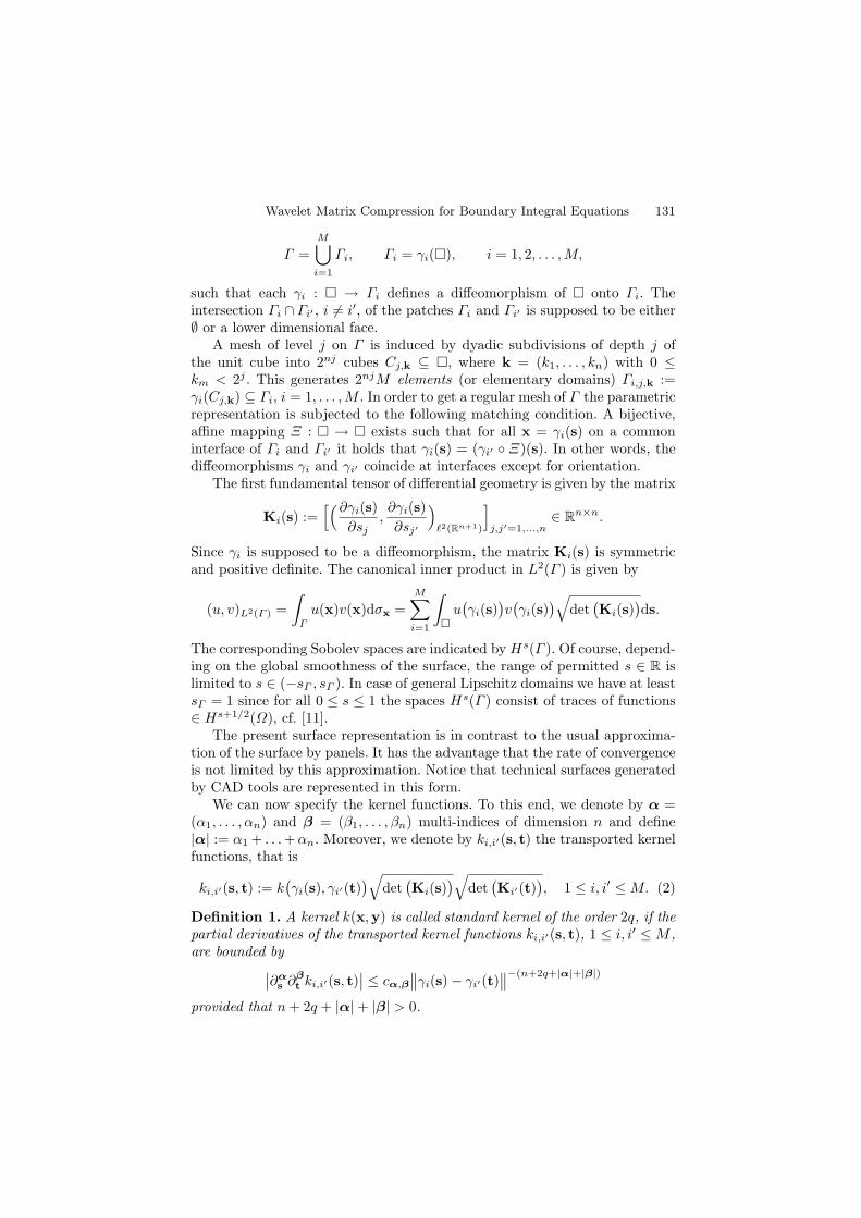
Wavelet Matrix Compression for Boundary Integral Equations 131
Γ =
M⋃
i=1
Γi, Γi = γi(), i = 1, 2, . . . ,M,
such that each γi : → Γi defines a diffeomorphism of onto Γi. Theintersection Γi ∩ Γi′ , i = i′, of the patches Γi and Γi′ is supposed to be either∅ or a lower dimensional face.
A mesh of level j on Γ is induced by dyadic subdivisions of depth j ofthe unit cube into 2nj cubes Cj,k ⊆ , where k = (k1, . . . , kn) with 0 ≤km < 2j . This generates 2njM elements (or elementary domains) Γi,j,k :=γi(Cj,k) ⊆ Γi, i = 1, . . . ,M . In order to get a regular mesh of Γ the parametricrepresentation is subjected to the following matching condition. A bijective,affine mapping Ξ : → exists such that for all x = γi(s) on a commoninterface of Γi and Γi′ it holds that γi(s) = (γi′ Ξ)(s). In other words, thediffeomorphisms γi and γi′ coincide at interfaces except for orientation.
The first fundamental tensor of differential geometry is given by the matrix
Ki(s) :=[(∂γi(s)
∂sj,∂γi(s)
∂sj′
)ℓ2(Rn+1)
]j,j′=1,...,n
∈ Rn×n.
Since γi is supposed to be a diffeomorphism, the matrix Ki(s) is symmetricand positive definite. The canonical inner product in L2(Γ ) is given by
(u, v)L2(Γ ) =
∫
Γ
u(x)v(x)dσx =
M∑
i=1
∫
u(γi(s)
)v(γi(s)
)√det
(Ki(s)
)ds.
The corresponding Sobolev spaces are indicated by Hs(Γ ). Of course, depend-ing on the global smoothness of the surface, the range of permitted s ∈ R islimited to s ∈ (−sΓ , sΓ ). In case of general Lipschitz domains we have at leastsΓ = 1 since for all 0 ≤ s ≤ 1 the spaces Hs(Γ ) consist of traces of functions∈ Hs+1/2(Ω), cf. [11].
The present surface representation is in contrast to the usual approxima-tion of the surface by panels. It has the advantage that the rate of convergenceis not limited by this approximation. Notice that technical surfaces generatedby CAD tools are represented in this form.
We can now specify the kernel functions. To this end, we denote by α =(α1, . . . , αn) and β = (β1, . . . , βn) multi-indices of dimension n and define|α| := α1 + . . .+αn. Moreover, we denote by ki,i′(s, t) the transported kernelfunctions, that is
ki,i′(s, t) := k(γi(s), γi′(t)
)√det
(Ki(s)
)√det
(Ki′(t)
), 1 ≤ i, i′ ≤M. (2)
Definition 1. A kernel k(x,y) is called standard kernel of the order 2q, if thepartial derivatives of the transported kernel functions ki,i′(s, t), 1 ≤ i, i′ ≤M ,are bounded by
∣∣∂αs ∂
βt ki,i′(s, t)
∣∣ ≤ cα,β
∥∥γi(s)− γi′(t)∥∥−(n+2q+|α|+|β|)
provided that n+ 2q + |α|+ |β| > 0.
132 Helmut Harbrecht et al.
We emphasize that this definition requires patchwise smoothness but notglobal smoothness of the geometry. The surface itself needs to be only Lip-schitz. Generally, under this assumption, the kernel of a boundary integraloperator A of order 2q is standard of order 2q. Hence, we may assume thisproperty in the sequel.
3 Wavelets and multiresolution analysis
In general, a multiresolution analysis consists of a nested family of finite di-mensional subspaces
Vj0+1 ⊂ Vj0+2 ⊂ · · · ⊂ Vj ⊂ Vj+1 · · · ⊂ · · · ⊂ L2(Γ ), (3)
such that dimVj ∼ 2jn and⋃
j>j0Vj = L2(Γ ). Each space Vj is defined
by a single-scale basis Φj = φj,k : k ∈ ∆j, i.e., Vj = spanΦj , where ∆j
denotes a suitable index set with cardinality |∆j | ∼ 2nj . It is convenient toidentify bases with row vectors, such that, for vj = [vj,k]k∈∆j
∈ ℓ2(∆j), thefunction vj = Φjvj is defined as vj =
∑k∈∆j
vj,kϕj,k. A final requirement
is that the bases Φj are uniformly stable, i.e., ‖vj‖ℓ2(∆j) ∼ ‖Φjvj‖L2(Γ ) forall vj ∈ ℓ2(∆j) uniformly in j. Furthermore, the single-scale bases satisfy thelocality condition diam suppφj,k ∼ 2−j .
If one is going to use the spaces Vj as trial spaces for the Galerkin schemethen additional properties are required. The trial spaces shall have approxi-mation order d ∈ N and regularity γ > 0, that is
γ = sups ∈ R : Vj ⊂ Hs(Γ ),d = sup
s ∈ R : inf
vj∈Vj
‖v − vj‖L2(Γ ) 2−js‖v‖Hs(Γ )
.
Note that conformity of the Galerkin scheme induces γ > q.Instead of using only a single-scale j the idea of wavelet concepts is to keep
track to increment of information between two adjacent scales j and j + 1.Since Vj ⊂ Vj+1 one decomposes Vj+1 = Vj ⊕Wj with some complementaryspaceWj ,Wj∩Vj = 0, not necessarily orthogonal to Vj . Of practical interestare the bases of the complementary spaces Wj in Vj+1
Ψj = ψj,k : k ∈ ∇j := ∆j+1 \∆j.
It is supposed that the collections Φj ∪ Ψj are also uniformly stable bases ofVj+1. If Ψ =
⋃j≥j0
Ψj , where Ψj0 := Φj0+1, is a Riesz-basis of L2(Γ ), we willcall it a wavelet basis. We assume the functions ψj,k to be local with respectto the corresponding scale j, i.e., diam suppψj,k ∼ 2−j , and we will normalizethem such that ‖ψj,k‖L2(Γ ) ∼ 1.
At first glance it would be very convenient to deal with a single ortho-normal system of wavelets. But it was shown in [13, 18, 47] that orthogonal
Wavelet Matrix Compression for Boundary Integral Equations 133
wavelets are not completely appropriate for the efficient solution of boundaryintegral equations. For that reason we use biorthogonal wavelet bases. Then,we have also a biorthogonal, or dual, multiresolution analysis, i.e., dual single-scale bases Φj = φj,k : k ∈ ∆j and wavelets Ψj = ψj,k : k ∈ ∆j which are
coupled to the primal ones via (Φj , Φj)L2(Γ ) = I and (Ψj , Ψj)L2(Γ ) = I. The
associated spaces Vj := span Φj and Wj := span Ψj satisfy
Vj ⊥ Wj , Vj ⊥Wj . (4)
Also the dual spaces shall have some approximation order d ∈ N and regularityγ > 0.
Denoting likewise to the primal side Ψ =⋃
j≥j0Ψj , where Ψj0 := Φj0+1,
then every v ∈ L2(Γ ) has a representation v = Ψ(v, Ψ)L2(Γ ) = Ψ(v, Ψ)L2(Γ ).Moreover, there hold the well known norm equivalences
‖v‖2Ht(Γ ) ∼∑
j≥j0
22jt‖(v, Ψj)L2(Γ )‖2ℓ2(∇j), t ∈ (−γ, γ),
‖v‖2Ht(Γ ) ∼∑
j≥j0
22jt‖(v, Ψj)L2(Γ )‖2ℓ2(∇j), t ∈ (−γ, γ).
(5)
The relation (4) implies that the wavelets provide vanishing moments of
order d ∣∣(v, ψj,k)L2(Γ )
∣∣ 2−j(d+n/2)|v|W d,∞(supp ψj,k). (6)
Here |v|W d,∞(Ω) := sup|α|=d, x∈Ω |∂αv(x)| denotes the semi-norm inW d,∞(Ω).
We refer to [12] for further details.
For the current type of boundary surfaces Γ the Φj , Φj are generated byconstructing first dual pairs of single-scale bases on the interval [0, 1], usingB-splines for the primal bases and the dual components from [9] adapted tothe interval [16]. Tensor products yield corresponding dual pairs on . Usingthe parametric liftings γi and gluing across patch boundaries leads to globallycontinuous single-scale bases Φj , Φj on Γ , [3,10,19,38]. For B-splines of order d
and duals of order d ≥ d such that d+ d is even the Φj , Φj have approximation
orders d, d, respectively. It is known that the respective regularity indices γ, γ(inside each patch) satisfy γ = d − 1/2 while γ > 0 is known to increase
proportionally to d. Appropriate wavelet bases are constructed by projecting astable completion into the correct complement spaces (see [4,19,31] for details).We refer the reader to [31, 36] for the details concerning the construction ofbiorthogonal wavelets on surfaces. Some illustrations are given in Fig. 1.
4 The wavelet Galerkin scheme
This section is devoted to a fully discrete wavelet Galerkin scheme for bound-ary integral equations. In the first subsection we discretize the given boundary
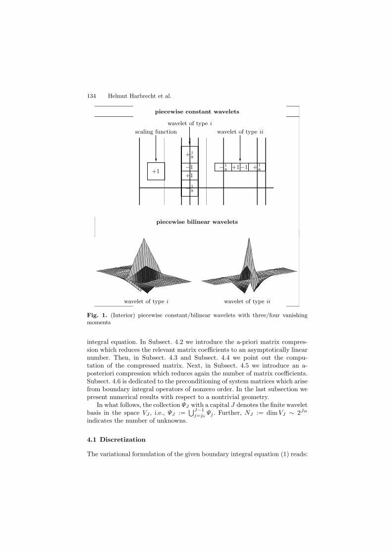
134 Helmut Harbrecht et al.
piecewise constant wavelets
scaling function
+1
wavelet of type i
+ 18
−1
+1
− 18
wavelet of type ii
− 18
+1−1 + 18
piecewise bilinear wavelets
wavelet of type i wavelet of type ii
Fig. 1. (Interior) piecewise constant/bilinear wavelets with three/four vanishingmoments
integral equation. In Subsect. 4.2 we introduce the a-priori matrix compres-sion which reduces the relevant matrix coefficients to an asymptotically linearnumber. Then, in Subsect. 4.3 and Subsect. 4.4 we point out the compu-tation of the compressed matrix. Next, in Subsect. 4.5 we introduce an a-posteriori compression which reduces again the number of matrix coefficients.Subsect. 4.6 is dedicated to the preconditioning of system matrices which arisefrom boundary integral operators of nonzero order. In the last subsection wepresent numerical results with respect to a nontrivial geometry.
In what follows, the collection ΨJ with a capital J denotes the finite waveletbasis in the space VJ , i.e., ΨJ :=
⋃J−1j=j0
Ψj . Further, NJ := dimVJ ∼ 2Jn
indicates the number of unknowns.
4.1 Discretization
The variational formulation of the given boundary integral equation (1) reads:
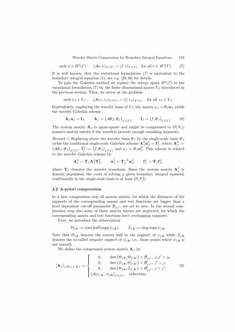
Wavelet Matrix Compression for Boundary Integral Equations 135
seek u ∈ Hq(Γ ) : (Au, v)L2(Γ ) = (f, v)L2(Γ ) for all v ∈ Hq(Γ ). (7)
It is well known, that the variational formulation (7) is equivalent to theboundary integral equation (1), see e.g. [28, 46] for details.
To gain the Galerkin method we replace the energy space Hq(Γ ) in thevariational formulation (7) by the finite dimensional spaces VJ introduced inthe previous section. Then, we arrive at the problem
seek uJ ∈ VJ : (AuJ , vJ )L2(Γ ) = (f, vJ )L2(Γ ) for all vJ ∈ VJ .
Equivalently, employing the wavelet basis of VJ , the ansatz uJ = ΨJuJ yieldsthe wavelet Galerkin scheme
AJuJ = fJ , AJ =(AΨJ , ΨJ
)L2(Γ )
, fJ =(f, ΨJ
)L2(Γ )
. (8)
The system matrix AJ is quasi-sparse and might be compressed to O(NJ )nonzero matrix entries if the wavelets provide enough vanishing moments.
Remark 1. Replacing above the wavelet basis ΨJ by the single-scale basis ΦJ
yields the traditional single-scale Galerkin scheme AφJuφ
J = fφJ , where Aφ
J :=(AΦJ , ΦJ
)L2(Γ )
, fφJ :=
(f, ΦJ
)L2(Γ )
and uJ = ΦJuφJ . This scheme is related
to the wavelet Galerkin scheme by
AψJ = TJAφ
JTTJ , uψ
J = T−TJ uφ
J , fψJ = TJ fφ
J ,
where TJ denotes the wavelet transform. Since the system matrix AφJ is
densely populated, the costs of solving a given boundary integral equationtraditionally in the single-scale basis is at least O(N2
J ).
4.2 A-priori compression
In a first compression step all matrix entries, for which the distances of thesupports of the corresponding ansatz and test functions are bigger than alevel dependent cut-off parameter Bj,j′ , are set to zero. In the second com-pression step also some of those matrix entries are neglected, for which thecorresponding ansatz and test functions have overlapping supports.
First, we introduce the abbreviation
Θj,k := conv hull(suppψj,k), Ξj,k := sing suppψj,k.
Note that Θj,k denotes the convex hull to the support of ψj,k while Ξj,k
denotes the so-called singular support of ψj,k, i.e., those points where ψj,k isnot smooth.
We define the compressed system matrix AJ by
[AJ ](j,k),(j′,k′) :=
0, dist(Θj,k, Θj′,k′
)> Bj,j′ , j, j′ > j0,
0, dist(Ξj,k, Θj′,k′
)> B′j,j′ , j′ > j,
0, dist(Θj,k, Ξj′,k′
)> B′j,j′ , j > j′,(
Aψj′,k′ , ψj,k
)L2(Γ )
, otherwise.
(9)
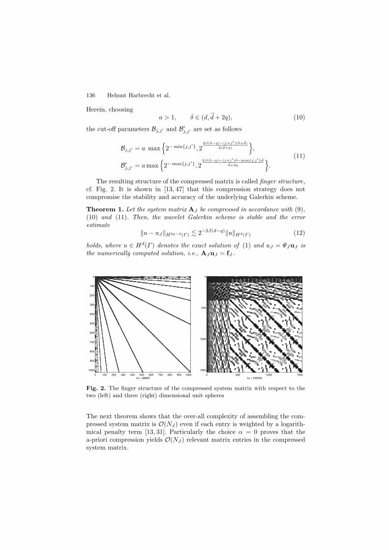
136 Helmut Harbrecht et al.
Herein, choosinga > 1, δ ∈ (d, d+ 2q), (10)
the cut-off parameters Bj,j′ and B′j,j′ are set as follows
Bj,j′ = a max
2−minj,j′, 22J(δ−q)−(j+j′)(δ+d)
2(d+q)
,
B′j,j′ = amax
2−maxj,j′, 22J(δ−q)−(j+j′)δ−maxj,j′d
d+2q
.
(11)
The resulting structure of the compressed matrix is called finger structure,cf. Fig. 2. It is shown in [13, 47] that this compression strategy does notcompromise the stability and accuracy of the underlying Galerkin scheme.
Theorem 1. Let the system matrix AJ be compressed in accordance with (9),(10) and (11). Then, the wavelet Galerkin scheme is stable and the errorestimate
‖u− uJ‖H2q−d(Γ ) 2−2J(d−q)‖u‖Hd(Γ ) (12)
holds, where u ∈ Hd(Γ ) denotes the exact solution of (1) and uJ = ΨJuJ isthe numerically computed solution, i.e., AJuJ = fJ .
0 100 200 300 400 500 600 700 800 900 1000
0
100
200
300
400
500
600
700
800
900
1000
nz = 668000 500 1000 1500
0
500
1000
1500
nz = 232520
Fig. 2. The finger structure of the compressed system matrix with respect to thetwo (left) and three (right) dimensional unit spheres
The next theorem shows that the over-all complexity of assembling the com-pressed system matrix is O(NJ ) even if each entry is weighted by a logarith-mical penalty term [13, 31]. Particularly the choice α = 0 proves that thea-priori compression yields O(NJ ) relevant matrix entries in the compressedsystem matrix.
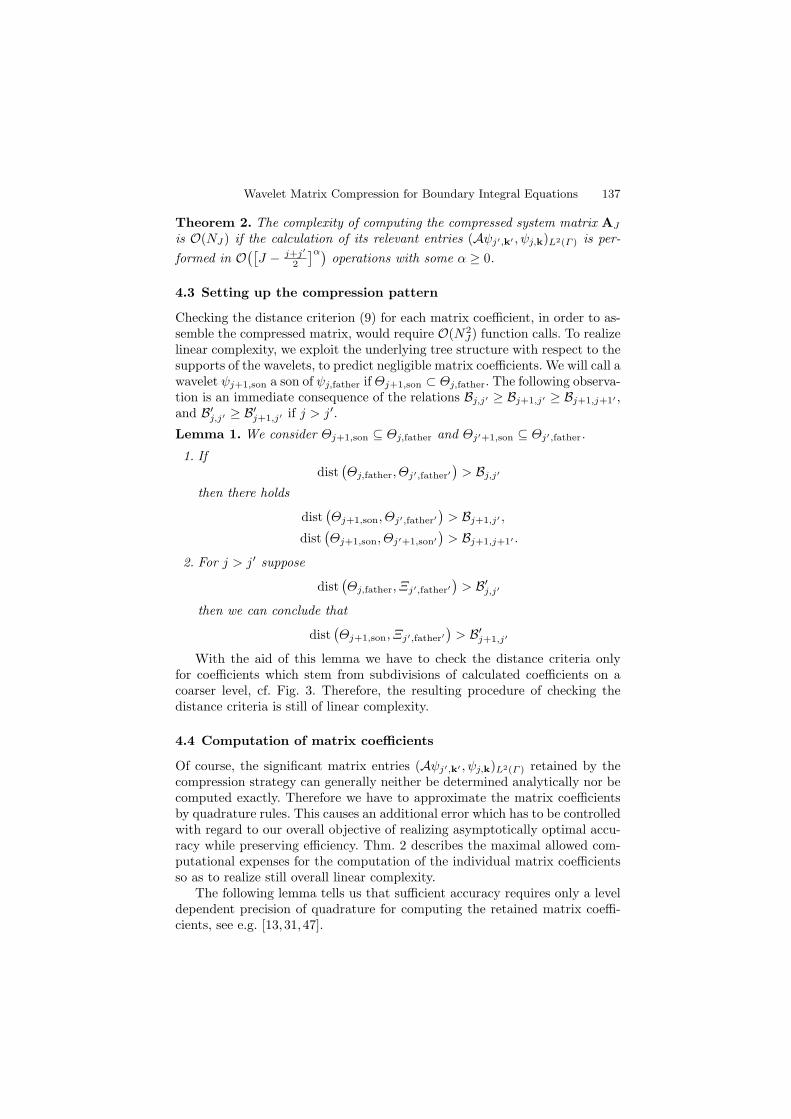
Wavelet Matrix Compression for Boundary Integral Equations 137
Theorem 2. The complexity of computing the compressed system matrix AJ
is O(NJ ) if the calculation of its relevant entries (Aψj′,k′ , ψj,k)L2(Γ ) is per-
formed in O([J − j+j′
2
]α)operations with some α ≥ 0.
4.3 Setting up the compression pattern
Checking the distance criterion (9) for each matrix coefficient, in order to as-semble the compressed matrix, would require O(N2
J ) function calls. To realizelinear complexity, we exploit the underlying tree structure with respect to thesupports of the wavelets, to predict negligible matrix coefficients. We will call awavelet ψj+1,son a son of ψj,father if Θj+1,son ⊂ Θj,father. The following observa-tion is an immediate consequence of the relations Bj,j′ ≥ Bj+1,j′ ≥ Bj+1,j+1′ ,and B′j,j′ ≥ B′j+1,j′ if j > j′.
Lemma 1. We consider Θj+1,son ⊆ Θj,father and Θj′+1,son ⊆ Θj′,father.
1. Ifdist
(Θj,father, Θj′,father′
)> Bj,j′
then there holds
dist(Θj+1,son, Θj′,father′
)> Bj+1,j′ ,
dist(Θj+1,son, Θj′+1,son′
)> Bj+1,j+1′ .
2. For j > j′ suppose
dist(Θj,father, Ξj′,father′
)> B′
j,j′
then we can conclude that
dist(Θj+1,son, Ξj′,father′
)> B′j+1,j′
With the aid of this lemma we have to check the distance criteria onlyfor coefficients which stem from subdivisions of calculated coefficients on acoarser level, cf. Fig. 3. Therefore, the resulting procedure of checking thedistance criteria is still of linear complexity.
4.4 Computation of matrix coefficients
Of course, the significant matrix entries (Aψj′,k′ , ψj,k)L2(Γ ) retained by thecompression strategy can generally neither be determined analytically nor becomputed exactly. Therefore we have to approximate the matrix coefficientsby quadrature rules. This causes an additional error which has to be controlledwith regard to our overall objective of realizing asymptotically optimal accu-racy while preserving efficiency. Thm. 2 describes the maximal allowed com-putational expenses for the computation of the individual matrix coefficientsso as to realize still overall linear complexity.
The following lemma tells us that sufficient accuracy requires only a leveldependent precision of quadrature for computing the retained matrix coeffi-cients, see e.g. [13, 31,47].
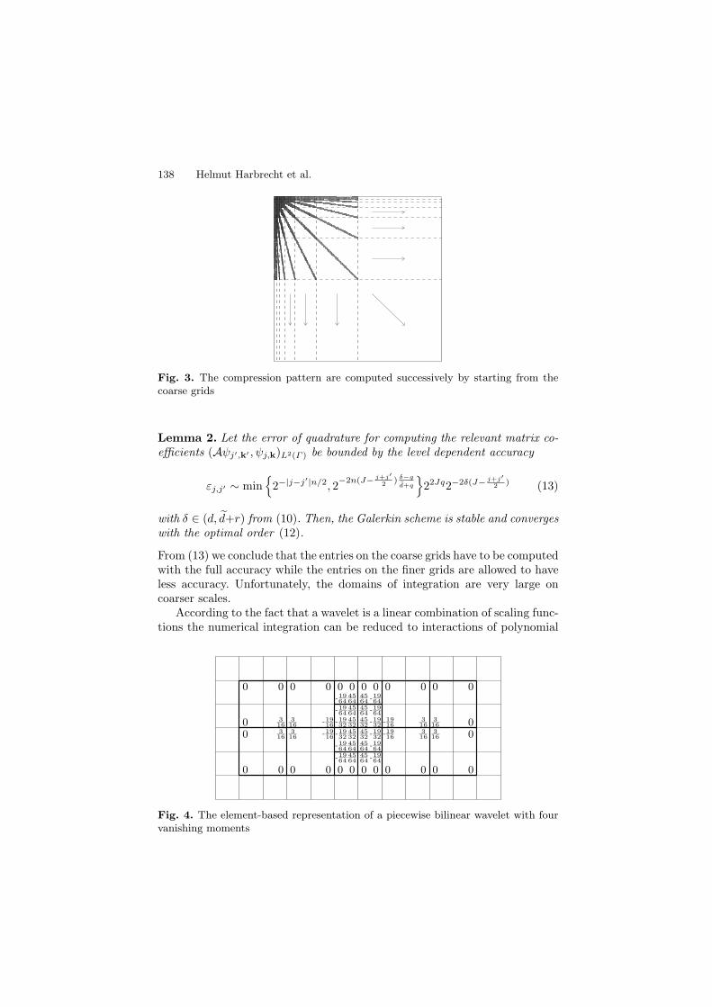
138 Helmut Harbrecht et al.
Fig. 3. The compression pattern are computed successively by starting from thecoarse grids
Lemma 2. Let the error of quadrature for computing the relevant matrix co-efficients (Aψj′,k′ , ψj,k)L2(Γ ) be bounded by the level dependent accuracy
εj,j′ ∼ min
2−|j−j′|n/2, 2−2n(J− j+j′
2 ) δ−q
d+q
22Jq2−2δ(J− j+j′
2 ) (13)
with δ ∈ (d, d+r) from (10). Then, the Galerkin scheme is stable and convergeswith the optimal order (12).
From (13) we conclude that the entries on the coarse grids have to be computedwith the full accuracy while the entries on the finer grids are allowed to haveless accuracy. Unfortunately, the domains of integration are very large oncoarser scales.
According to the fact that a wavelet is a linear combination of scaling func-tions the numerical integration can be reduced to interactions of polynomial
0 0 0 0 0 00 0 0 0 0 0
-1964
4564
4564
-1964
-1964
4564
4564
-1964
0 316
-1932
4532
-1916
316
316
-1916
4532
-1932
316 0
0 316
-1932
4532
-1916
316
316
-1916
4532
-1932
316 0
-1964
4564
4564
-1964
-1964
4564
4564
-1964
0 0 0 0 0 00 0 0 0 0 0
Fig. 4. The element-based representation of a piecewise bilinear wavelet with fourvanishing moments
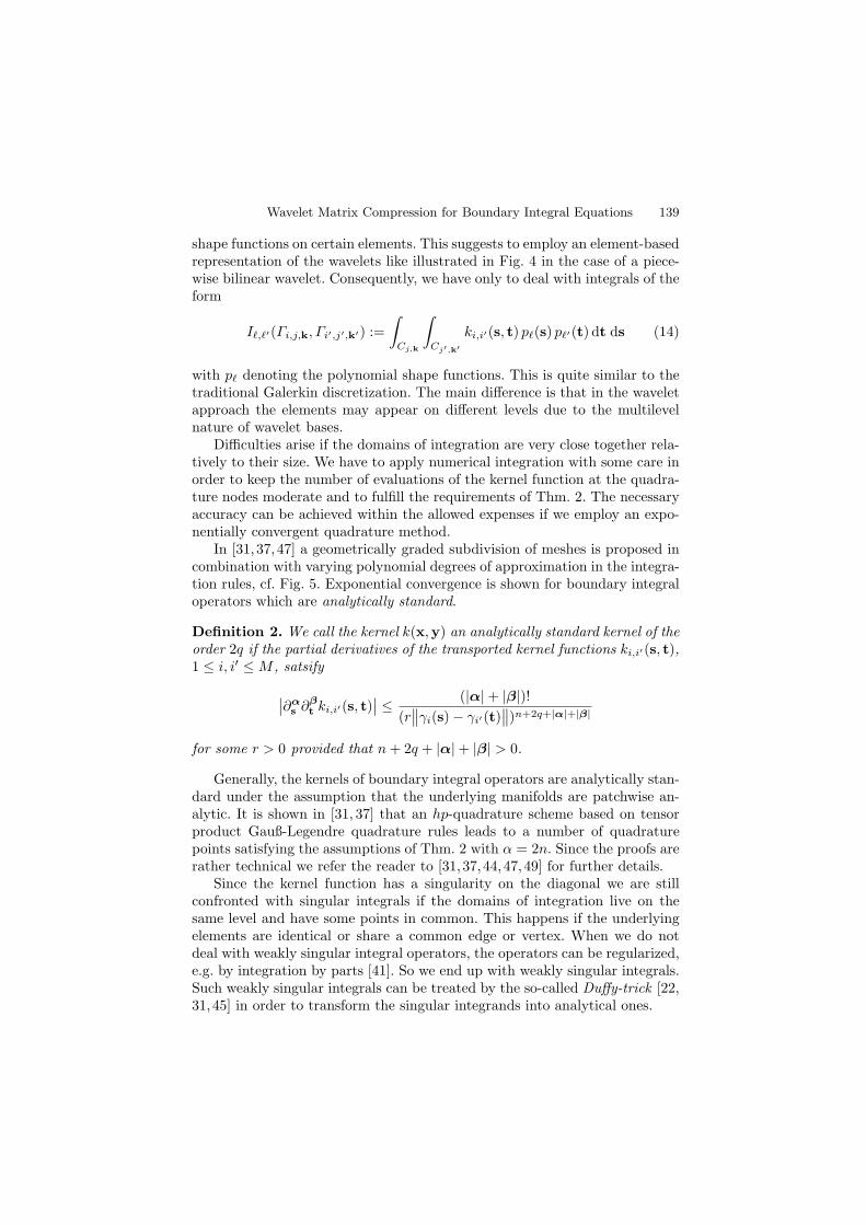
Wavelet Matrix Compression for Boundary Integral Equations 139
shape functions on certain elements. This suggests to employ an element-basedrepresentation of the wavelets like illustrated in Fig. 4 in the case of a piece-wise bilinear wavelet. Consequently, we have only to deal with integrals of theform
Iℓ,ℓ′(Γi,j,k, Γi′,j′,k′) :=
∫
Cj,k
∫
Cj′,k′
ki,i′(s, t) pℓ(s) pℓ′(t) dt ds (14)
with pℓ denoting the polynomial shape functions. This is quite similar to thetraditional Galerkin discretization. The main difference is that in the waveletapproach the elements may appear on different levels due to the multilevelnature of wavelet bases.
Difficulties arise if the domains of integration are very close together rela-tively to their size. We have to apply numerical integration with some care inorder to keep the number of evaluations of the kernel function at the quadra-ture nodes moderate and to fulfill the requirements of Thm. 2. The necessaryaccuracy can be achieved within the allowed expenses if we employ an expo-nentially convergent quadrature method.
In [31, 37, 47] a geometrically graded subdivision of meshes is proposed incombination with varying polynomial degrees of approximation in the integra-tion rules, cf. Fig. 5. Exponential convergence is shown for boundary integraloperators which are analytically standard.
Definition 2. We call the kernel k(x,y) an analytically standard kernel of theorder 2q if the partial derivatives of the transported kernel functions ki,i′(s, t),1 ≤ i, i′ ≤M , satsify
∣∣∂αs ∂
βt ki,i′(s, t)
∣∣ ≤ (|α|+ |β|)!(r∥∥γi(s)− γi′(t)
∥∥)n+2q+|α|+|β|
for some r > 0 provided that n+ 2q + |α|+ |β| > 0.
Generally, the kernels of boundary integral operators are analytically stan-dard under the assumption that the underlying manifolds are patchwise an-alytic. It is shown in [31, 37] that an hp-quadrature scheme based on tensorproduct Gauß-Legendre quadrature rules leads to a number of quadraturepoints satisfying the assumptions of Thm. 2 with α = 2n. Since the proofs arerather technical we refer the reader to [31,37,44,47,49] for further details.
Since the kernel function has a singularity on the diagonal we are stillconfronted with singular integrals if the domains of integration live on thesame level and have some points in common. This happens if the underlyingelements are identical or share a common edge or vertex. When we do notdeal with weakly singular integral operators, the operators can be regularized,e.g. by integration by parts [41]. So we end up with weakly singular integrals.Such weakly singular integrals can be treated by the so-called Duffy-trick [22,31,45] in order to transform the singular integrands into analytical ones.
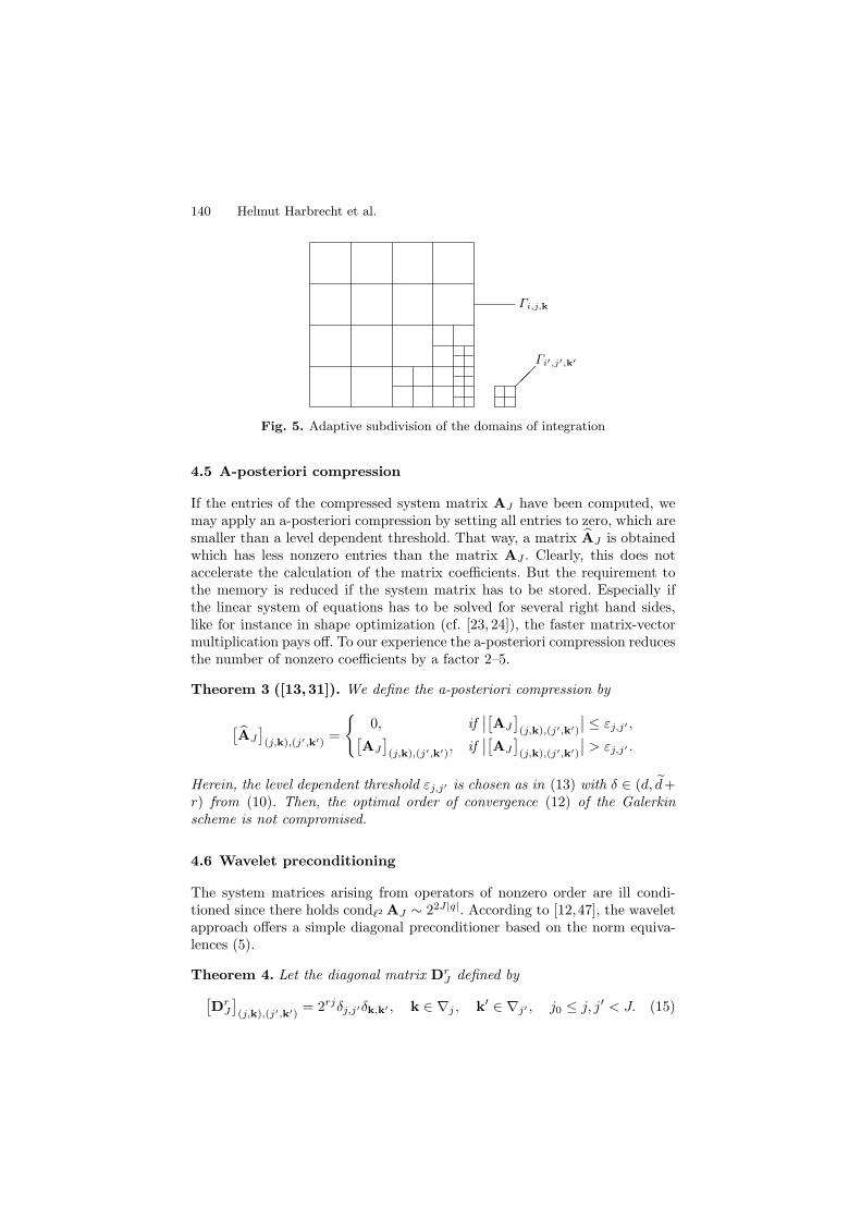
140 Helmut Harbrecht et al.
Γi′,j′,k′
Γi,j,k
Fig. 5. Adaptive subdivision of the domains of integration
4.5 A-posteriori compression
If the entries of the compressed system matrix AJ have been computed, wemay apply an a-posteriori compression by setting all entries to zero, which aresmaller than a level dependent threshold. That way, a matrix AJ is obtainedwhich has less nonzero entries than the matrix AJ . Clearly, this does notaccelerate the calculation of the matrix coefficients. But the requirement tothe memory is reduced if the system matrix has to be stored. Especially ifthe linear system of equations has to be solved for several right hand sides,like for instance in shape optimization (cf. [23, 24]), the faster matrix-vectormultiplication pays off. To our experience the a-posteriori compression reducesthe number of nonzero coefficients by a factor 2–5.
Theorem 3 ([13,31]). We define the a-posteriori compression by
[AJ
](j,k),(j′,k′)
=
0, if
∣∣[AJ
](j,k),(j′,k′)
∣∣ ≤ εj,j′ ,[AJ
](j,k),(j′,k′)
, if∣∣[AJ
](j,k),(j′,k′)
∣∣ > εj,j′ .
Herein, the level dependent threshold εj,j′ is chosen as in (13) with δ ∈ (d, d+r) from (10). Then, the optimal order of convergence (12) of the Galerkinscheme is not compromised.
4.6 Wavelet preconditioning
The system matrices arising from operators of nonzero order are ill condi-tioned since there holds condℓ2 AJ ∼ 22J|q|. According to [12,47], the waveletapproach offers a simple diagonal preconditioner based on the norm equiva-lences (5).
Theorem 4. Let the diagonal matrix DrJ defined by
[Dr
J
](j,k),(j′,k′)
= 2rjδj,j′δk,k′ , k ∈ ∇j , k′ ∈ ∇j′ , j0 ≤ j, j′ < J. (15)
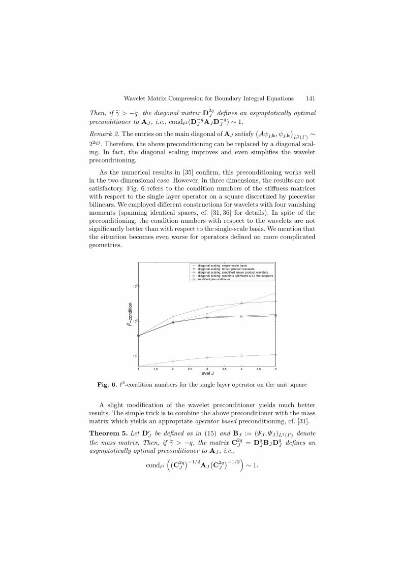
Wavelet Matrix Compression for Boundary Integral Equations 141
Then, if γ > −q, the diagonal matrix D2qJ defines an asymptotically optimal
preconditioner to AJ , i.e., condℓ2(D−qJ AJD−q
J ) ∼ 1.
Remark 2. The entries on the main diagonal of AJ satisfy(Aψj,k, ψj,k
)L2(Γ )
∼22qj . Therefore, the above preconditioning can be replaced by a diagonal scal-ing. In fact, the diagonal scaling improves and even simplifies the waveletpreconditioning.
As the numerical results in [35] confirm, this preconditioning works wellin the two dimensional case. However, in three dimensions, the results are notsatisfactory. Fig. 6 refers to the condition numbers of the stiffness matriceswith respect to the single layer operator on a square discretized by piecewisebilinears. We employed different constructions for wavelets with four vanishingmoments (spanning identical spaces, cf. [31, 36] for details). In spite of thepreconditioning, the condition numbers with respect to the wavelets are notsignificantly better than with respect to the single-scale basis. We mention thatthe situation becomes even worse for operators defined on more complicatedgeometries.
1 1.5 2 2.5 3 3.5 4 4.5 5
101
102
103
level J
l2−
con
diti
on
diagonal scaling: single−scale basisdiagonal scaling: tensor product waveletsdiagonal scaling: simplified tensor product waveletsdiagonal scaling: wavelets optimized w.r.t. the supportsmodified preconditioner
Fig. 6. ℓ2-condition numbers for the single layer operator on the unit square
A slight modification of the wavelet preconditioner yields much betterresults. The simple trick is to combine the above preconditioner with the massmatrix which yields an appropriate operator based preconditioning, cf. [31].
Theorem 5. Let DrJ be defined as in (15) and BJ := (ΨJ , ΨJ)L2(Γ ) denote
the mass matrix. Then, if γ > −q, the matrix C2qJ = Dq
JBJDqJ defines an
asymptotically optimal preconditioner to AJ , i.e.,
condℓ2
((C2q
J
)−1/2AJ
(C2q
J
)−1/2)∼ 1.

142 Helmut Harbrecht et al.
This preconditioner decreases the condition numbers impressively, cf. Fig. 6.Moreover, the condition depends now only on the underlying spaces but not onthe chosen wavelet basis. To our experiences the condition reduces about thefactor 10–100 compared to the preconditioner (15). We like to mention that,employing the fast wavelet transform, the application of this preconditionerrequires only the inversion of a single-scale mass matrix, which is diagonal incase of piecewise constant and very sparse in case of piecewise bilinear ansatzfunctions.
4.7 Numerical results
Let Ω be the gearwheel shown in Fig. 7, represented by 504 patches. We seekthe function U ∈ H1(Ω) satisfying the interior Dirichlet problem
∆U = 0 in Ω, U = 1 on Γ . (16)
The ansatz
U(x) =1
4π
∫
Γ
u(y)
‖x− y‖dσy, x ∈ Ω, (17)
yields the Fredholm boundary integral equation of the first kind Vu = 1 forthe unknown density function u. Herein, V : H−1/2(Γ ) → H1/2(Γ ) denotesthe single layer operator given by
(Vu)(x) :=1
4π
∫
Γ
u(y)
‖x− y‖dσy, x ∈ Γ. (18)
Fig. 7. The mesh on the surface Γ and the evaluation points xi
We discretize the given boundary integral equation by piecewise constantwavelets with three vanishing moments which is consistent to (10). We com-pute the discrete solution UJ := [UJ (xi)] according to (17) from the approx-imated density uJ , where the evaluation points xi are specified in Fig. 7.If the density u is in H1(Γ ) we obtain for x ∈ Ω the pointwise estimate|U(x)− UJ(x)| ≤ cx‖u− uJ‖H−2(Γ ) 2−3J‖u‖H1(Γ ), cf. [54]. Unfortunately,
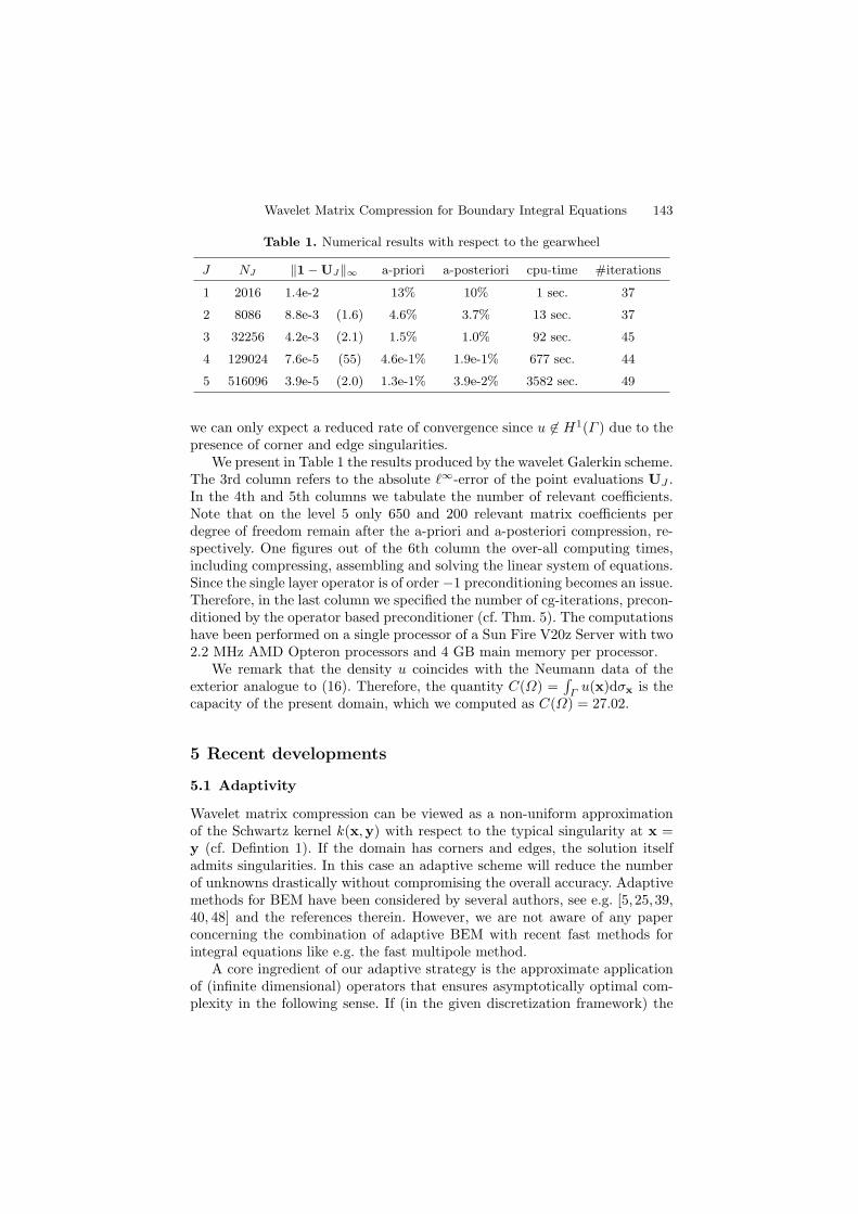
Wavelet Matrix Compression for Boundary Integral Equations 143
Table 1. Numerical results with respect to the gearwheel
J NJ ‖1 − UJ‖∞ a-priori a-posteriori cpu-time #iterations
1 2016 1.4e-2 13% 10% 1 sec. 37
2 8086 8.8e-3 (1.6) 4.6% 3.7% 13 sec. 37
3 32256 4.2e-3 (2.1) 1.5% 1.0% 92 sec. 45
4 129024 7.6e-5 (55) 4.6e-1% 1.9e-1% 677 sec. 44
5 516096 3.9e-5 (2.0) 1.3e-1% 3.9e-2% 3582 sec. 49
we can only expect a reduced rate of convergence since u ∈ H1(Γ ) due to thepresence of corner and edge singularities.
We present in Table 1 the results produced by the wavelet Galerkin scheme.The 3rd column refers to the absolute ℓ∞-error of the point evaluations UJ .In the 4th and 5th columns we tabulate the number of relevant coefficients.Note that on the level 5 only 650 and 200 relevant matrix coefficients perdegree of freedom remain after the a-priori and a-posteriori compression, re-spectively. One figures out of the 6th column the over-all computing times,including compressing, assembling and solving the linear system of equations.Since the single layer operator is of order−1 preconditioning becomes an issue.Therefore, in the last column we specified the number of cg-iterations, precon-ditioned by the operator based preconditioner (cf. Thm. 5). The computationshave been performed on a single processor of a Sun Fire V20z Server with two2.2 MHz AMD Opteron processors and 4 GB main memory per processor.
We remark that the density u coincides with the Neumann data of theexterior analogue to (16). Therefore, the quantity C(Ω) =
∫Γu(x)dσx is the
capacity of the present domain, which we computed as C(Ω) = 27.02.
5 Recent developments
5.1 Adaptivity
Wavelet matrix compression can be viewed as a non-uniform approximationof the Schwartz kernel k(x,y) with respect to the typical singularity at x =y (cf. Defintion 1). If the domain has corners and edges, the solution itselfadmits singularities. In this case an adaptive scheme will reduce the numberof unknowns drastically without compromising the overall accuracy. Adaptivemethods for BEM have been considered by several authors, see e.g. [5,25,39,40, 48] and the references therein. However, we are not aware of any paperconcerning the combination of adaptive BEM with recent fast methods forintegral equations like e.g. the fast multipole method.
A core ingredient of our adaptive strategy is the approximate applicationof (infinite dimensional) operators that ensures asymptotically optimal com-plexity in the following sense. If (in the given discretization framework) the

144 Helmut Harbrecht et al.
unknown solution u can be approximated in the energy norm with an opti-mal choice of N degrees of freedom at a rate N−s, then the adaptive schemematches this rate by producing for any target accuracy ε an approximate so-lution uε such that ‖u− uε‖Hq(Γ ) ≤ ε at a computational expense that stays
proportionally to ε−1/s as ε tends to zero, see [6, 7]. Notice that N−s, wheres := (d − q)/n, is the best possible rate of convergence, gained in case ofuniform refinement if u ∈ Hd(Γ ). Since the computation of the relevant ma-trix coefficients is by far the most expensive step in our algorithm, we cannotuse the approach of [6, 7]. In [14] we adopted the strategy of the best N -termapproximation by the notion of tree approximation, as considered in [8, 21].
The algorithm is based on an iterative method for the continuous equation(1), expanded with respect to the wavelet basis. To this end we assume thewavelet basis Ψ to be normalized in the energy space. Then, (1) is equivalentto the well posed problem of finding u = Ψu such that the infinite dimensionallinear system of equations
Au = f , A = (AΨ, Ψ)L2(Γ ), f = (f, Ψ)L2(Γ ), (19)
holds. The application of the operator to a function is approximated by anappropriate (finite dimensional) matrix-vector multiplication. Given a finitelysupported vector v and a target accuracy ε, we choose wavelet trees τj ac-cording to
‖v − v|τ‖ℓ2 ≤ 2jsε, j = 0, 1, . . . , J :=
⌈log2(‖v‖ℓ2/ε)
s
⌉
and define the layers ∆j := τj+1 \ τj . These layers play now the role of thelevels in case of the non-adaptive scheme, i.e. we will balance the accuracylayer-dependent. We adopt the compression rules defined in [50] to defineoperators Aj , having only O(2j(1 + j)−2(n+1)) relevant coefficients per rowand column while satisfying
‖A−Aj‖ℓ2 ≤2−js
(1 + j)2(n+1).
Then, the approximate matrix-vector multiplication
w :=
J−1∑
j=0
Ajv|∆j
gives raise to the estimate ‖Av−w‖ℓ2 ≤ ε. Combing this approximate matrix-vector product with an suitable iterative solver for (19) (cf. [6]) or the adaptiveGalerkin type algorithm from [26] we achieve the desired goal of optimalcomplexity. We refer the reader to [14] for the details.
Wavelet Matrix Compression for Boundary Integral Equations 145
5.2 Wavelet matrix compression for complex geometries
If the geometry is given as collection πiNi=1 of piecewise polygonal panels,which is quite common for the treatment of complex geometries, we cannot usethe previous approach since the multiscale hierarchy (3) is realized by refine-ment. However, following [51], by agglomeration we can construct piecewiseconstant wavelets that are orthogonal to polynomials in the space
∫
Γ
ψj,k(x)xαdσx = 0, |α| < d. (20)
To this end, we have to introduce a hierarchical non-overlapping subdivision ofthe boundary Γ , called the cluster tree T (see Fig. 8). The cluster-tree shouldbe a balanced 2n tree of depth J , such that that we have approximately 2jn
clusters ν per level j with size diam ν ∼ 2−j . Then, starting on the finestlevel J with the piecewise constant ansatz functions Φπi
J := φi, we definescaling functions Φν
j = φνj,k and wavelets Ψν
j = ψνj,k of a cluster ν on
level j recursively via[Φν
j , Ψνj
]= Φν
j+1
[Vν
j,Φ,Vνj,Ψ
]. The coefficient matrices
Vνj,φ and Vν
j,ψ are computed via singular value decomposition of the momentmatrices
Mνj :=
[∫
Γ
xαΦνj+1(x)dσ
]
|α|<d
= UΣVT = U [S,0][Vν
j,Φ,Vνj,Ψ
]T,
see [51] for details. Therefore, we obtain a multiscale hierarchy with respect tothe spaces Vj := spanΦν
j : ν is cluster of level j. The spacesWj := spanΨνj :
ν is cluster of level j satisfy Vj+1 = Vj⊕Wj , in particular Vj ⊥Wj due to theorthogonality of
[Vν
j,Φ,Vνj,Ψ
]. Hence, we can define an orthonormal wavelet
basis by ΨN := ΦΓ0 ∪ Ψν
j : ν ∈ T. In [32] the authors proved the normequivalences (5) in a range (−1/2, 1/2).
The cancellation property (20) is stronger than (6) since no smoothnessof the manifold is required. Therefore, we can weaken the assumptions on thekernel. The kernel function k(x,y) is supposed to be analytical in the spacevariables x,y ∈ R
n+1, apart from the singularity x = y, satisfying the decayproperty
|∂αx ∂
βy k(x,y)| α!β!
(r‖x− y‖)n+2q+|α|+|β|
for some r > 0 uniformly in the (n + 1)-dimensional multi-indices α and β.Of practical interest in our considerations are first kind Fredholm integralequations for the single layer operator (q = −1/2) and second kind Fredholmintegral equations for the double layer operator (q = 0).
The system matrix becomes again quasi-sparse in wavelet coordinates pro-vided that d > d− 2q. Since this time the wavelets are not smooth, only thefirst compression in (9) applies which results in O(N logN) relevant matrixcoefficients. In Fig. 9 one finds the system matrix (left) and its sparsity pat-tern (right). In case of the single layer operator the proven norm equivalences
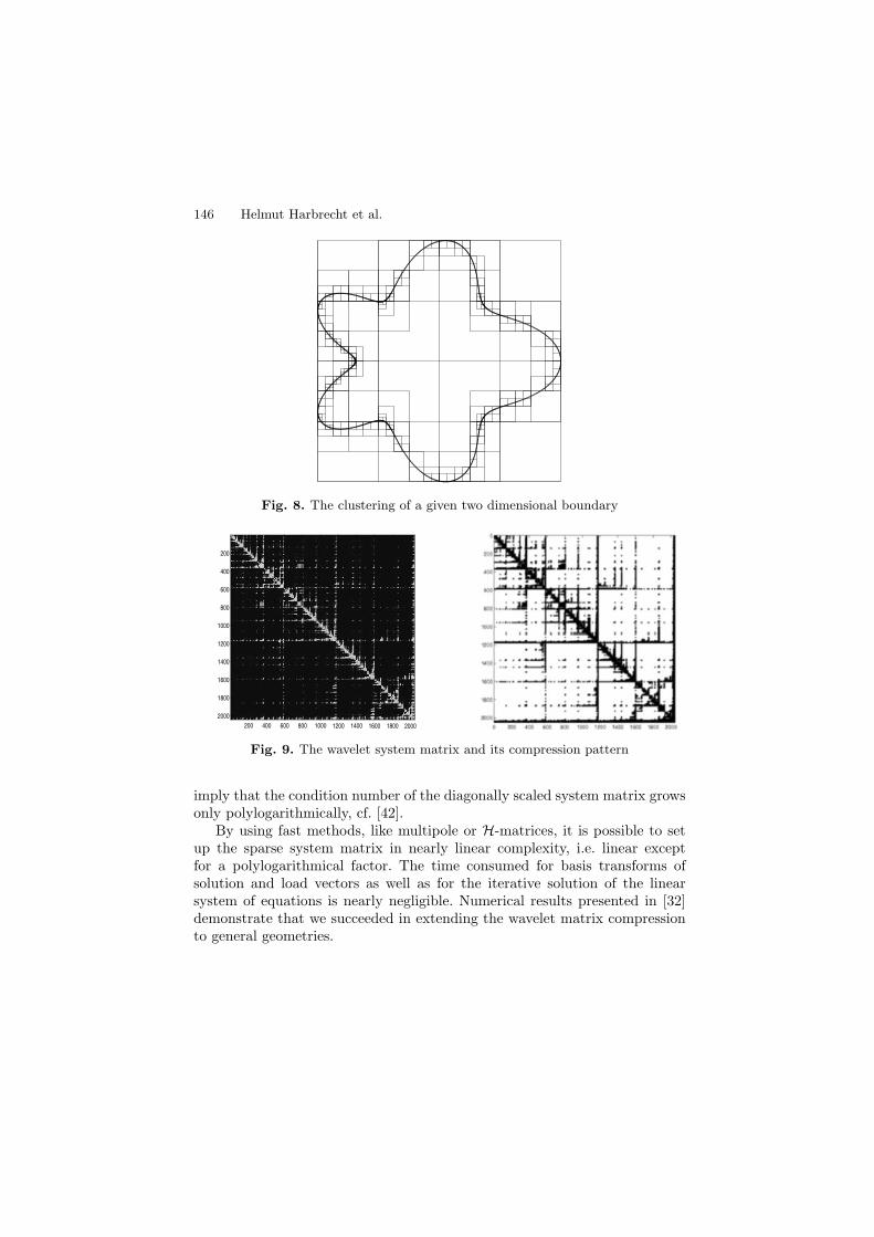
146 Helmut Harbrecht et al.
Fig. 8. The clustering of a given two dimensional boundary
200 400 600 800 1000 1200 1400 1600 1800 2000
200
400
600
800
1000
1200
1400
1600
1800
2000
Fig. 9. The wavelet system matrix and its compression pattern
imply that the condition number of the diagonally scaled system matrix growsonly polylogarithmically, cf. [42].
By using fast methods, like multipole or H-matrices, it is possible to setup the sparse system matrix in nearly linear complexity, i.e. linear exceptfor a polylogarithmical factor. The time consumed for basis transforms ofsolution and load vectors as well as for the iterative solution of the linearsystem of equations is nearly negligible. Numerical results presented in [32]demonstrate that we succeeded in extending the wavelet matrix compressionto general geometries.
Wavelet Matrix Compression for Boundary Integral Equations 147
References
1. M. Bebendorf and S. Rjasanow. Adaptive low-rank approximation of collocationmatrices. Computing, 70:1–24, 2003.
2. G. Beylkin, R. Coifman, and V. Rokhlin. The fast wavelet transform and nu-merical algorithms. Comm. Pure and Appl. Math., 44:141–183, 1991.
3. C. Canuto, A. Tabacco, and K. Urban. The wavelet element method, part I:Construction and analysis. Appl. Comput. Harm. Anal., 6:1–52, 1999.
4. J. Carnicer, W. Dahmen, and J. Pena. Local decompositions of refinable spaces.Appl. Comp. Harm. Anal., 3:127–153, 1996.
5. C. Carstensen and E.P. Stephan. Adaptive boundary element methods for somefirst kind integral equations. SIAM J. Numer. Anal., 33:2166–2183, 1996.
6. A. Cohen, W. Dahmen, and R. DeVore. Adaptive Wavelet Methods for EllipticOperator Equations – Convergence Rates. Math. Comp., 70:27–75, 2001.
7. A. Cohen, W. Dahmen, and R. DeVore. Adaptive Wavelet Methods II – Beyondthe Elliptic Case. Found. Comput. Math., 2:203–245, 2002.
8. A. Cohen, W. Dahmen, and R. DeVore. Adaptive wavelet schemes for nonlinearvariational problems. SIAM J. Numer. Anal., 41:1785–1823, 2003.
9. A. Cohen, I. Daubechies, and J.-C. Feauveau. Biorthogonal bases of compactlysupported wavelets. Pure Appl. Math., 45:485–560, 1992.
10. A. Cohen and R. Masson. Wavelet adaptive method for second order ellipticproblems – boundary conditions and domain decomposition. Numer. Math.,86:193–238, 2000.
11. M. Costabel. Boundary integral operators on Lipschitz domains: Elementaryresults. SIAM J. Math. Anal., 19:613–626, 1988.
12. W. Dahmen. Wavelet and multiscale methods for operator equations. ActaNumerica, 6:55–228, 1997.
13. W. Dahmen, H. Harbrecht, and R. Schneider. Compression techniques forboundary integral equations – optimal complexity estimates. SIAM J. Numer.Anal., 43:2251–2271, 2006.
14. W. Dahmen, H. Harbrecht and R. Schneider. Adaptive Methods for BoundaryIntegral Equations – Complexity and Convergence Estimates. IGPM Report #250, RWTH Aachen, Germany, 2005. submitted to Math. Comp.
15. W. Dahmen, B. Kleemann, S. Proßdorf, and R. Schneider. A multiscale methodfor the double layer potential equation on a polyhedron. In H.P. Dikshit andC.A. Micchelli, editors, Advances in Computational Mathematics, pages 15–57,World Scientific Publ., Singapore, 1994.
16. W. Dahmen, A. Kunoth, and K. Urban. Biorthogonal spline-wavelets on theinterval – stability and moment conditions. Appl. Comp. Harm. Anal., 6:259–302, 1999.
17. W. Dahmen, S. Proßdorf, and R. Schneider. Wavelet approximation methodsfor periodic pseudodifferential equations. Part II – Matrix compression and fastsolution. Adv. Comput. Math., 1:259–335, 1993.
18. W. Dahmen, S. Proßdorf, and R. Schneider. Multiscale methods for pseudo-differential equations on smooth closed manifolds. In C.K. Chui, L. Montefusco,and L. Puccio, editors, Proceedings of the International Conference on Wavelets:Theory, Algorithms, and Applications, pages 385–424, 1994.
19. W. Dahmen and R. Schneider. Composite wavelet bases for operator equations.Math. Comp., 68:1533–1567, 1999.
148 Helmut Harbrecht et al.
20. W. Dahmen and R. Schneider. Wavelets on manifolds I. Construction anddomain decomposition. Math. Anal., 31:184–230, 1999.
21. W. Dahmen, R. Schneider, and Y. Xu. Nonlinear functionals of waveletexpansions—adaptive reconstruction and fast evaluation. Numer. Math., 86:49–101, 2000.
22. M. Duffy. Quadrature over a pyramid or cube of integrands with a singularityat the vertex. SIAM J. Numer. Anal., 19:1260–1262, 1982.
23. K. Eppler and H. Harbrecht. 2nd Order Shape Optimization using WaveletBEM. Optim. Methods Softw., 21:135–153, 2006.
24. K. Eppler and H. Harbrecht. Efficient treatment of stationary free boundaryproblems. WIAS-Preprint 965, WIAS Berlin, Germany, 2004. to appear inAppl. Numer. Math.
25. B. Faermann. Local a-posteriori error indicators for the Galerkin discretizationof boundary integral equations. Numer. Math., 79:43–76, 1998.
26. T. Gantumur, H. Harbrecht, and R. Stevenson. An Optimal Adaptive WaveletMethod Without Coarsening. Preprint No. 1325, Department of Mathematics,Universiteit Utrecht, The Netherlands, 2005. to appear in Math. Comp.
27. L. Greengard and V. Rokhlin. A fast algorithm for particle simulation. J.Comput. Phys., 73:325–348, 1987.
28. W. Hackbusch. Integral equations. Theory and numerical treatment. Interna-tional Series of Numerical Mathematics, volume 120, Birkhauser Verlag, Basel,1995.
29. W. Hackbusch. A sparse matrix arithmetic based on H-matrices. Part I: Intro-duction to H-matrices. Computing, 64:89–108, 1999.
30. W. Hackbusch and Z.P. Nowak. On the fast matrix multiplication in the bound-ary element method by panel clustering. Numer. Math., 54:463–491, 1989.
31. H. Harbrecht. Wavelet Galerkin schemes for the boundary element method inthree dimensions. PHD Thesis, Technische Universitat Chemnitz, Germany,2001.
32. H. Harbrecht, U. Kahler, and R. Schneider. Wavelet Galerkin BEM on unstruc-tured meshes. Comput. Vis. Sci., 8:189–199, 2005.
33. H. Harbrecht, F. Paiva, C. Perez, and R. Schneider. Biorthogonal wavelet ap-proximation for the coupling of FEM-BEM. Numer. Math., 92:325–356, 2002.
34. H. Harbrecht, F. Paiva, C. Perez, and R. Schneider. Wavelet preconditioningfor the coupling of FEM-BEM. Num. Lin. Alg. Appl., 10:197–222, 2003.
35. H. Harbrecht and R. Schneider. Wavelet Galerkin Schemes for 2D-BEM. InJ. Elschner, I. Gohberg and B. Silbermann, editors, Problems and methods inmathematical physics, Operator Theory: Advances and Applications, volume121, pages 221–260, Birkhauser Verlag, Basel, 2001.
36. H. Harbrecht and R. Schneider. Biorthogonal wavelet bases for the boundaryelement method. Math. Nachr., 269–270:167–188, 2004.
37. H. Harbrecht and R. Schneider. Wavelet Galerkin Schemes for Boundary IntegralEquations – Implementation and Quadrature. SIAM J. Sci. Comput., 27:1347–1370, 2006.
38. H. Harbrecht and R. Stevenson. Wavelets with patchwise cancellation proper-ties. Preprint No. 1311, Department of Mathematics, Universiteit Utrecht, TheNetherlands, 2004. to appear in Math. Comp.
39. M. Maischak, P. Mund, and E.P. Stephan. Adaptive multilevel BEM foracoustic scattering. Symposium on Advances in Computational Mechanics,
Wavelet Matrix Compression for Boundary Integral Equations 149
Vol. 2, (Austin, TX, 1997). Comput. Methods Appl. Mech. Engrg., 150:351–367, 1997.
40. P. Mund, and E.P. Stephan. An adaptive two-level method for hypersingu-lar integral equations in R3. Proceedings of the 1999 International Confer-ence on Computational Techniques and Applications (Canberra). ANZIAM J.,42:C1019–C1033, 2000.
41. J.-C. Nedelec. Acoustic and Electromagnetic Equations — Integral Representa-tions for Harmonic Problems. Springer Verlag, 2001.
42. P. Oswald: Multilevel norms for H−1/2. Computing, 61:235–255, 1998.43. T. von Petersdorff, R. Schneider, and C. Schwab. Multiwavelets for second kind
integral equations. SIAM J. Num. Anal., 34:2212–2227, 1997.44. T. von Petersdorff and C. Schwab. Fully discretized multiscale Galerkin BEM.
In W. Dahmen, A. Kurdila, and P. Oswald, editors, Multiscale wavelet methodsfor PDEs, pages 287–346, Academic Press, San Diego, 1997.
45. S. Sauter and C. Schwab. Quadrature for the hp-Galerkin BEM in R3. Numer.
Math., 78:211–258, 1997.46. S. Sauter and C. Schwab. Randelementmethoden. Analyse, Numerik und Imple-
mentierung schneller Algorithmen. B.G. Teubner, Stuttgart, 1997.47. R. Schneider. Multiskalen- und Wavelet-Matrixkompression: Analysisbasierte
Methoden zur Losung großer vollbesetzter Gleichungssysteme. B.G. Teubner,Stuttgart, 1998.
48. H. Schulz and O. Steinbach. A new a posteriori error estimator in adaptivedirect boundary element methods. The Dirichlet problem. Calcolo, 37:79–96,2000.
49. C. Schwab. Variable order composite quadrature of singular and nearly singularintegrals. Computing, 53:173–194, 1994.
50. R. Stevenson: On the compressibility of operators in wavelet coordinates. SIAMJ. Math. Anal., 35:1110–1132, 2004.
51. J. Tausch and J. White: Multiscale bases for the sparse representation of bound-ary integral operators on complex geometries. SIAM J. Sci. Comput., 24:1610–1629, 2003.
52. E.E. Tyrtyshnikov. Mosaic sceleton approximation. Calcolo, 33:47–57, 1996.53. L. Villemoes. Wavelet analysis of refinement equations. SIAM J. Math. Anal.,
25:1433–1460, 1994.54. W.L. Wendland. On asymptotic error analysis and underlying mathematical
principles for boundary element methods. In C.A. Brebbia, editor, BoundaryElement Techniques in Computer Aided Engineering, NATO ASI Series E-84,pages 417–436, Martinus Nijhoff Publ., Dordrecht-Boston-Lancaster, 1984.

Numerical Solution of Optimal ControlProblems for Parabolic Systems
Peter Benner1, Sabine Gorner1, and Jens Saak1
Technische Universitat Chemnitz, Fakultat fur Mathematik09107 Chemnitz, Germanybenner,sabine.goerner,[email protected]
1 Introduction
We consider nonlinear parabolic diffusion-convection and diffusion-reactionsystems of the form
∂x
∂t+∇ · (c(x)− k(∇x)) + q(x) = Bu(t), t ∈ [0, Tf ], (1)
in Ω ∈ Rd, d = 1, 2, 3, with appropriate initial and boundary conditions. Here,
c is the convective part, k the diffusive part and q is an uncontrolled sourceterm. The state of the system depends on ξ ∈ Ω and the time t ∈ [0, Tf ] andis denoted by x(ξ, t). The control is called u(t) and is assumed to depend onlyon the time t ∈ [0, Tf ].
A control problem is defined as
minuJ(x,u) subject to (1), (2)
where J(x,u) is a performance index which will be introduced later.There are two possibilities for the appearance of the control. If the control
occurs in the boundary condition, we call this problem a boundary controlproblem. It is called distributed control problem if the control acts in Ω ora sub-domain Ωu ⊂ Ω. The control problem as in (1) is well-suited to de-scribe a distributed control problem while boundary control will require thespecification of the boundary conditions as, for instance, given below.
The major part of this article deals with the linear version of (1),
∂x
∂t−∇. (a(ξ)∇x) + d(ξ)∇x + r(ξ)x = BV (ξ)u(t), ξ ∈ Ω, t > 0, (3)
with initial and boundary conditions
152 Peter Benner et al.
α(ξ)∂x(ξ, t)
∂n+ γ(ξ)x(ξ, t) = BRu(t), ξ ∈ ∂Ω,
x(ξ, 0) = x0(ξ), ξ ∈ Ω,
for sufficiently smooth parameters a, d, r, α, γ,x0. We assume that eitherBV = 0 (boundary control system) or BR = 0 (distributed control system).In addition, we include in our problem an output equation of the form
y = Cx, t ≥ 0,
taking into account that in practice, often not the whole state x is availablefor measurements. Here, C is a linear operator which often is a restrictionoperator.
To solve optimal control problems (2) with a linear system (3) we interpretit as a linear quadratic regulator (LQR) problem. The theory behind the LQRansatz has already been studied in detail, e.g., in [1–6], to name only a few.
Nonlinear control problems are still undergoing extensive research. We willapply model predictive control (MPC) here, i.e., we solve linearized problemson small time frames using a linear-quadratic Gaussian (LQG) design. Thisidea is presented by Ito and Kunisch in [7]. We will briefly sketch the mainideas of this approach at the end of this article.
There exists a rich variety of other approaches to solve linear and nonlinearoptimal control problems for partial differential equations. We can only referto a selection of ideas, see e.g. [4, 8–12].
This article is divided into four parts. In the remainder of this section wewill give a short introduction to linear control problems and we present themodel problem used in this article. Theoretical results which justify the nu-merical implementation of the LQR problem will be pointed out in Sect. 2.The third section deals with computational methods for the model problem.There we go into algorithmic and implementation details and present somenumerical results. Finally we give an insight into a method for nonlinear par-abolic systems in Sect. 4.
1.1 Linear problems
In this section we will formulate the linear quadratic regulator (LQR) problem.We assume that X ,Y,U are separable Hilbert spaces where X is called thestate space, Y the observation space and U the control space.
Furthermore the linear operators
A : dom(A) ⊂ X → X ,B : U → X ,C : X → Y
are given. Such an abstract system can now be understood as a Cauchy prob-lem for a linear evolution equation of the form
Numerical Solution of Optimal Control Problems for Parabolic Systems 153
x = Ax + Bu, x(., 0) = x0 ∈ X . (4)
Since in many applications the state x of a system can not be observed com-pletely we consider the observation equation
y = Cx, (5)
which describes the map between the states and the outputs of the system.The abstract LQR problem is now given as the minimization problem
minu∈L2(0,Tf ;U)
1
2
Tf∫
0
〈y,Qy〉Y + 〈u,Ru〉U dt (6)
with self-adjoint, positive definite, linear, bounded operators Q and R onY and U , respectively. Recall that if (4) is an ordinary differential equationwith X = R
n, Y = Rp and U = R
m, equipped with the standard scalarproduct, then we obtain an LQR problem for a finite-dimensional system[13]. For partial differential equations we have to choose the function spacesX ,Y,U appropriately and we get an LQR system for an infinite-dimensionalsystem [14, 15].
Many optimal control problems for instationary linear partial differentialequations can be described using the abstract LQR problem above. Addition-ally, many control, stabilization and parameter identification problems can bereduced to the LQR problem, see [1–3,15,16].
The infinite time case
In the infinite time case we assume that Tf = ∞. Then the minimizationproblem subject to (4) is given by
minu∈L2(0,∞;U)
1
2
∞∫
0
〈y,Qy〉Y + 〈u,Ru〉U dt. (7)
If the standard assumptions that
• A is the infinitesimal generator of a C0-semigroup T(t),• B,C are linear bounded operators and• for every initial value there exists an admissible control u ∈ L2(0,∞;U)
hold then the solution of the abstract LQR problem can be obtained analo-gously to the finite-dimensional case (see [14,17,18]). We then have to considerthe algebraic operator Riccati equation
0 = ℜ(P) = C∗QC + A∗P + PA−PBR−1B∗P, (8)
154 Peter Benner et al.
where the linear operator P will be the solution of (8) if P : domA→ domA∗
and 〈x,ℜ(P)x〉 = 0 for all x, x ∈ dom(A). The optimal control is then givenas the feedback control
u∗(t) = −R−1B∗P∞x∗(t), (9)
which has the form of a regulator or closed-loop control. Here, P∞ is theminimal nonnegative self-adjoint solution of (8), x∗(t) = S(t)x0(t), and S(t)is the C0-semigroup generated by A−BR−1B∗P∞. Using further standardassumptions it can be shown, see e.g. [5], that P∞ is the unique nonnegativesolution of (8). Most of the required conditions, particularly the restrictiveassumption that B is bounded, can be weakened [1, 2].
The finite time case
The finite time case arises if Tf < ∞ in (6). Then the numerical solutionis more complicated since we have to solve the operator differential Riccatiequation
P(t) = −(C∗QC + A∗P(t) + P(t)A−P(t)BR−1B∗P(t)). (10)
The optimal control is obtained as
u∗(t) = −R−1B∗P∗(t)x∗(t),
where P∗(t) is the unique solution of (10) in complete analogy to the infinitetime case in (9).
1.2 Discretization
For the discretization of an optimal control problem we can follow differentstrategies. In the literature the following two alternatives are often used:
• “Optimize–then–discretize”That is, we compute the optimal control with methods of optimizationfirst and discretize afterwards.
• “Discretize–then–optimize”Here, we discretize at first and optimize the discrete problem.
The literature provides a large amount of approaches which are based onnon-smooth Newton’s methods or sequential quadratic programming (SQP)methods, see, e.g., [11, 12,19].
In contrast to the strategies above we want to examine the strategy“semidiscretize–optimize–semidiscretize”. If we semidiscretize in space first,for instance by using a Galerkin ansatz with finite element ansatz functions,we obtain a linear finite-dimensional system. The structure and solution of theresulting system are analogous to those of the infinite dimensional system.
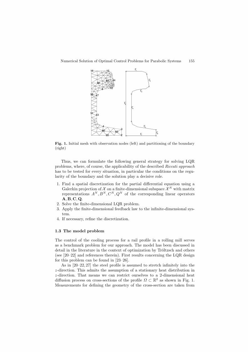
Numerical Solution of Optimal Control Problems for Parabolic Systems 155
0
1
2
3
4
5
67
Γ
Γ
Γ
Γ
Γ
Γ
ΓΓ2
34
9 10
1516
22
34
43
47
51
55
60 63
8392
Fig. 1. Initial mesh with observation nodes (left) and partitioning of the boundary(right)
Thus, we can formulate the following general strategy for solving LQRproblems, where, of course, the applicability of the described Riccati approachhas to be tested for every situation, in particular the conditions on the regu-larity of the boundary and the solution play a decisive role.
1. Find a spatial discretization for the partial differential equation using aGalerkin projection of X on a finite-dimensional subspace XN with matrixrepresentations AN , BN , CN , QN of the corresponding linear operatorsA,B,C,Q.
2. Solve the finite-dimensional LQR problem.3. Apply the finite-dimensional feedback law to the infinite-dimensional sys-
tem.4. If necessary, refine the discretization.
1.3 The model problem
The control of the cooling process for a rail profile in a rolling mill servesas a benchmark problem for our approach. The model has been discussed indetail in the literature in the context of optimization by Troltzsch and others(see [20–22] and references therein). First results concerning the LQR designfor this problem can be found in [23–26].
As in [20–22, 27] the steel profile is assumed to stretch infinitely into thez-direction. This admits the assumption of a stationary heat distribution inz-direction. That means we can restrict ourselves to a 2-dimensional heatdiffusion process on cross-sections of the profile Ω ⊂ R
2 as shown in Fig. 1.Measurements for defining the geometry of the cross-section are taken from
156 Peter Benner et al.
[20]. As one can see in Fig. 1 the domain exploits the symmetry of the profileintroducing an artificial boundary Γ0 on the symmetry axis.
We will concentrate on the linearized version of the state equation intro-duced in [20–22]. The linearization is derived by taking means of the materialparameters ρ, λ and c. This is admissible as long as we work in temperatureregimes above approximately 700-800 (depending on the kind of steel used)where changes of ρ, λ and c are small and we do not have multiple phasesand phase transitions in the material. We partition the non-artificial bound-ary into 7 parts, each of them located between two neighboring corners of thedomain (see Fig. 1 for details). The control u is assumed to be constant withrespect to the spatial variable ξ on each part Γi of the boundary. Thus weobtain the following model:
cρ∂x(ξ,t)∂t = ∇.(λ∇x(ξ, t)) in Ω × (0, T ),
−λ∂x(ξ,t)∂n = gi(t, x, u) on Γi for i = 0, . . . , 7,
x(ξ, 0) = x0(ξ) in Ω.
(11)
We now have to describe the heat transfer across the surface of the mate-rial, i.e. the boundary conditions. The boundary condition according to New-ton’s cooling law is given as
−∂x(ξ, t)∂n
=κk
λ(x(ξ, t)− xext,k(t)). (12)
Note that xext,k(t) is assumed to be constant on Γk and therefore does notdepend explicitly on ξ. For a more detailed derivation of this condition see [26].
Here, we will take the external temperature as the control. The mathe-matical advantage of this choice is that the multiplication of control and statewhich would lead to a bilinear control system in case of the heat transfercoefficient as control is avoided.
2 Theoretical results
2.1 Approximation of abstract cauchy problems
The theoretical fundament for our approach was set by Gibson [18]. The ideasand proofs used for the boundary control problem considered here closely fol-low the extension of Gibson’s method proposed by Banks and Kunisch [28]for distributed control systems arising from parabolic equations. Similar ap-proaches can be found in [2,26]. Common to all those approaches is to formu-late the control system for a parabolic system as an abstract Cauchy problemin an appropriate Hilbert space setting. For numerical approaches this Hilbertspace X is approximated by a sequence of finite-dimensional spaces (XN )N∈N,e.g., by spatial finite element approximations, leading to large sparse systems
Numerical Solution of Optimal Control Problems for Parabolic Systems 157
of ordinary differential equations in Rn. Following the theory in [28] those
approximations do not even have to be subspaces of the Hilbert space of so-lutions.
Before stating the main theoretical result we will first collect some approx-imation prerequisites we will need for the theorem. We call them (BK1) and(BK2) for they were already formulated in [28] (and called H1 and H2 there).In the following ΠN is the canonical projection operator mapping from theinfinite-dimensional space X to its finite-dimensional approximation XN . Thefirst and natural prerequisite is:
For each N and x0 ∈ XN there exists an admissible controluN ∈ L2(0,∞;U) and any admissible control drives the statesto 0 asymptotically.
(BK1)
Additionally one needs the following properties for the approximation asN → ∞. Assume that for each N , AN is the infinitesimal generator of aC0-semigroup TN (t), then we require:
(i) For all ϕ ∈ X we have uniform convergenceTN (t)ΠNϕ → T(t)ϕ on any bounded subintervalof [0,∞).
(ii) For all φ ∈ X we have uniform convergenceTN (t)∗ΠNφ → T(t)∗φ on any bounded subintervalof [0,∞).
(iii) For all v ∈ U we have BNv → Bv and for all ϕ ∈ X wehave BN ∗
ϕ→ B∗ϕ.
(iv) For all ϕ ∈ X we have QNΠNϕ→ Qϕ.
(BK2)
With these we can now formulate the main result.
Theorem 1 (Convergence of the finite-dimensional approximations).Let (BK1) and (BK2) hold. Moreover, assume R > 0, Q ≥ 0 and QN ≥ 0.Further, let PN be the solutions of the AREs for the finite-dimensional systemsand let the minimal nonnegative self-adjoint solution P of (8) for (4), (5) and(7) exist. Moreover, let S(t) and SN (t) be the operator semigroups generatedby A−BR−1B∗P on X and AN −BNR−1BN ∗
PN on XN , respectively, with‖S(t)ϕ‖ → 0 as t→∞ for all ϕ ∈ X .
If there exist positive constants M1, M2 and ω independent of N and t,such that
‖SN (t)‖XN ≤ M1e−ωt,
‖PN‖XN ≤ M2,(13)
then
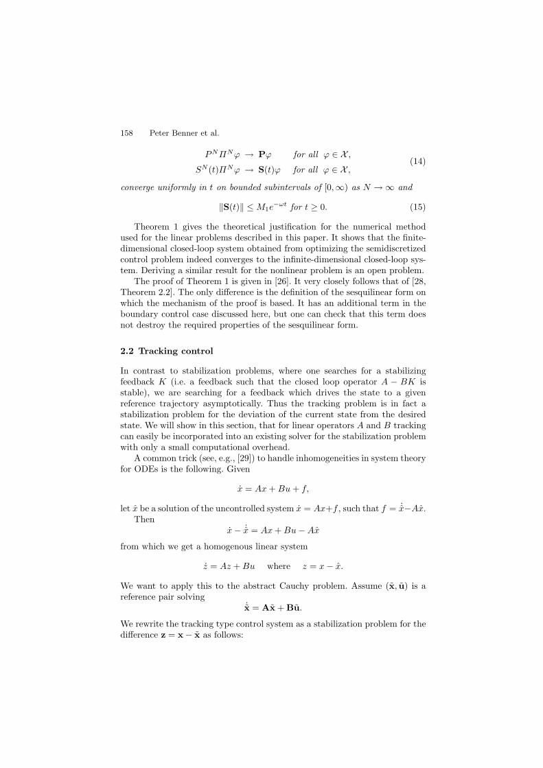
158 Peter Benner et al.
PNΠNϕ → Pϕ for all ϕ ∈ X ,SN (t)ΠNϕ → S(t)ϕ for all ϕ ∈ X ,
(14)
converge uniformly in t on bounded subintervals of [0,∞) as N →∞ and
‖S(t)‖ ≤M1e−ωt for t ≥ 0. (15)
Theorem 1 gives the theoretical justification for the numerical methodused for the linear problems described in this paper. It shows that the finite-dimensional closed-loop system obtained from optimizing the semidiscretizedcontrol problem indeed converges to the infinite-dimensional closed-loop sys-tem. Deriving a similar result for the nonlinear problem is an open problem.
The proof of Theorem 1 is given in [26]. It very closely follows that of [28,Theorem 2.2]. The only difference is the definition of the sesquilinear form onwhich the mechanism of the proof is based. It has an additional term in theboundary control case discussed here, but one can check that this term doesnot destroy the required properties of the sesquilinear form.
2.2 Tracking control
In contrast to stabilization problems, where one searches for a stabilizingfeedback K (i.e. a feedback such that the closed loop operator A − BK isstable), we are searching for a feedback which drives the state to a givenreference trajectory asymptotically. Thus the tracking problem is in fact astabilization problem for the deviation of the current state from the desiredstate. We will show in this section, that for linear operators A and B trackingcan easily be incorporated into an existing solver for the stabilization problemwith only a small computational overhead.
A common trick (see, e.g., [29]) to handle inhomogeneities in system theoryfor ODEs is the following. Given
x = Ax+Bu+ f,
let x be a solution of the uncontrolled system x = Ax+f , such that f = ˙x−Ax.Then
x− ˙x = Ax+Bu−Axfrom which we get a homogenous linear system
z = Az +Bu where z = x− x.
We want to apply this to the abstract Cauchy problem. Assume (x, u) is areference pair solving
˙x = Ax + Bu.
We rewrite the tracking type control system as a stabilization problem for thedifference z = x− x as follows:
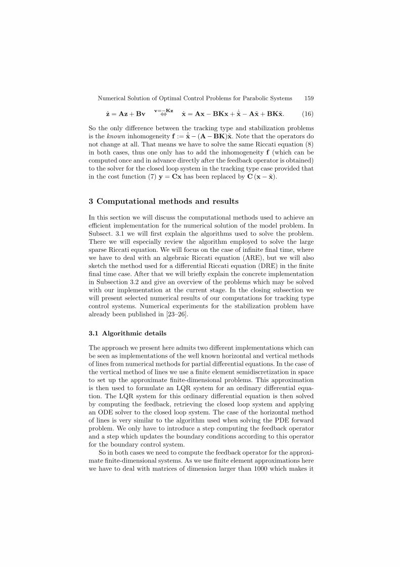
Numerical Solution of Optimal Control Problems for Parabolic Systems 159
z = Az + Bvv=−Kz⇔ x = Ax−BKx + ˙x−Ax + BKx. (16)
So the only difference between the tracking type and stabilization problemsis the known inhomogeneity f := ˙x− (A−BK)x. Note that the operators donot change at all. That means we have to solve the same Riccati equation (8)in both cases, thus one only has to add the inhomogeneity f (which can becomputed once and in advance directly after the feedback operator is obtained)to the solver for the closed loop system in the tracking type case provided thatin the cost function (7) y = Cx has been replaced by C (x− x).
3 Computational methods and results
In this section we will discuss the computational methods used to achieve anefficient implementation for the numerical solution of the model problem. InSubsect. 3.1 we will first explain the algorithms used to solve the problem.There we will especially review the algorithm employed to solve the largesparse Riccati equation. We will focus on the case of infinite final time, wherewe have to deal with an algebraic Riccati equation (ARE), but we will alsosketch the method used for a differential Riccati equation (DRE) in the finitefinal time case. After that we will briefly explain the concrete implementationin Subsection 3.2 and give an overview of the problems which may be solvedwith our implementation at the current stage. In the closing subsection wewill present selected numerical results of our computations for tracking typecontrol systems. Numerical experiments for the stabilization problem havealready been published in [23–26].
3.1 Algorithmic details
The approach we present here admits two different implementations which canbe seen as implementations of the well known horizontal and vertical methodsof lines from numerical methods for partial differential equations. In the case ofthe vertical method of lines we use a finite element semidiscretization in spaceto set up the approximate finite-dimensional problems. This approximationis then used to formulate an LQR system for an ordinary differential equa-tion. The LQR system for this ordinary differential equation is then solvedby computing the feedback, retrieving the closed loop system and applyingan ODE solver to the closed loop system. The case of the horizontal methodof lines is very similar to the algorithm used when solving the PDE forwardproblem. We only have to introduce a step computing the feedback operatorand a step which updates the boundary conditions according to this operatorfor the boundary control system.
So in both cases we need to compute the feedback operator for the approxi-mate finite-dimensional systems. As we use finite element approximations herewe have to deal with matrices of dimension larger than 1000 which makes it
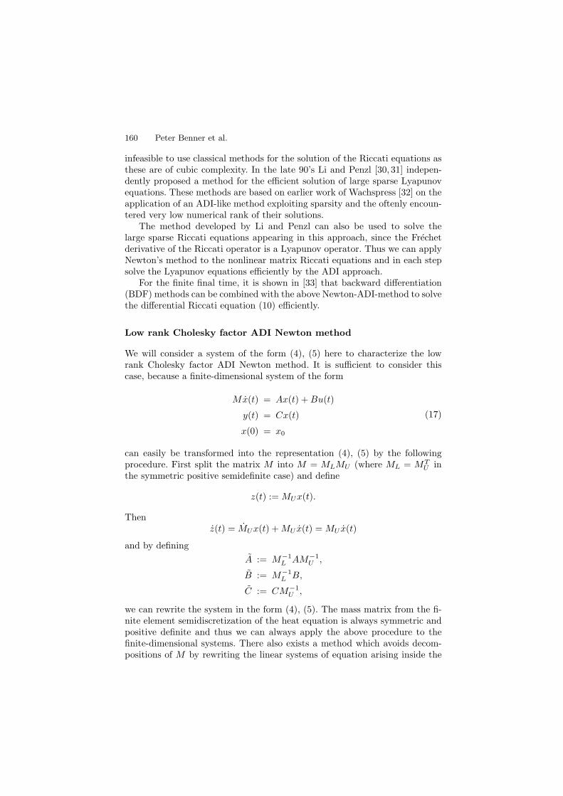
160 Peter Benner et al.
infeasible to use classical methods for the solution of the Riccati equations asthese are of cubic complexity. In the late 90’s Li and Penzl [30, 31] indepen-dently proposed a method for the efficient solution of large sparse Lyapunovequations. These methods are based on earlier work of Wachspress [32] on theapplication of an ADI-like method exploiting sparsity and the oftenly encoun-tered very low numerical rank of their solutions.
The method developed by Li and Penzl can also be used to solve thelarge sparse Riccati equations appearing in this approach, since the Frechetderivative of the Riccati operator is a Lyapunov operator. Thus we can applyNewton’s method to the nonlinear matrix Riccati equations and in each stepsolve the Lyapunov equations efficiently by the ADI approach.
For the finite final time, it is shown in [33] that backward differentiation(BDF) methods can be combined with the above Newton-ADI-method to solvethe differential Riccati equation (10) efficiently.
Low rank Cholesky factor ADI Newton method
We will consider a system of the form (4), (5) here to characterize the lowrank Cholesky factor ADI Newton method. It is sufficient to consider thiscase, because a finite-dimensional system of the form
Mx(t) = Ax(t) +Bu(t)
y(t) = Cx(t)
x(0) = x0
(17)
can easily be transformed into the representation (4), (5) by the followingprocedure. First split the matrix M into M = MLMU (where ML = MT
U inthe symmetric positive semidefinite case) and define
z(t) :=MUx(t).
Thenz(t) = MUx(t) +MU x(t) =MU x(t)
and by defining
A := M−1L AM−1
U ,
B := M−1L B,
C := CM−1U ,
we can rewrite the system in the form (4), (5). The mass matrix from the fi-nite element semidiscretization of the heat equation is always symmetric andpositive definite and thus we can always apply the above procedure to thefinite-dimensional systems. There also exists a method which avoids decom-positions of M by rewriting the linear systems of equation arising inside the

Numerical Solution of Optimal Control Problems for Parabolic Systems 161
Fig. 2. Data flow in the horizontal (left) and vertical (right) method of lines imple-mentations
ADI method instead of the control system (see [34] for details). We discussedthe above method in detail here, because it is used in the LyaPack softwarepackage used to solve the Riccati equations in our implementation.
The low rank Cholesky factor ADI Newton method implemented in Lya-
Pack can be seen as a modification of the classical Newton-like method foralgebraic Riccati equations (Kleinman iteration, [35]), where the Lyapunovsubproblems in each Newton step are solved by the low rank Cholesky factorADI method. The most important feature of this method is that it does notwork with the generally full n × n iterates Xi but with low rank Choleskyfactors thereof (ZiZ
Ti = Xi). The rank of Zi is generally full but it has ri ≪ n
columns which drastically reduces memory consumption and computationalcomplexity. LyaPack also provides functions iterating directly on the rectan-gular (number of rows = number of system inputs ≪ n) feedback matrixpossibly reducing the complexity even further.
3.2 Implementation details
For the implementation we combine the software packages LyaPack1 (see [36])and ALBERTA2 (see [37]). LyaPack is a collection of Matlab-routines forsolving large-scale Lyapunov equations, LQR problems, and model reductiontasks. Therefore we used Matlab to initialize the computation. That meanswe setup the initial control parameters and the time measurement routines ata Matlab-console. After that the finite element discretization is generatedby a mex call to a C-function utilizing the finite element method (fem) libraryALBERTA. Inside this routine the system matricesM , A and B are assembled.After system assembly the program returns to the Matlab prompt providingthe matrices and problem data like current time and temperature profile. Nowthe matrices C, Q, and R are initialized and LyaPack is used to compute thefeedback matrix.
1available from: http://www.tu-chemnitz.de/2available from: http://www.alberta-fem.de

162 Peter Benner et al.
0.0000
39327.50
1.0001.000
0.8750
0.5000
0.7500
0.6250
0.5000
0.0000
39327.50
1.000
0.5000
0.6250
0.7500
0.8750
1.000
0.5000
Fig. 3. Initial (left) and final (right) temperature distribution for a tracking typesystem steering to constant 700
In case of the horizontal method of lines the program now returns tothe ALBERTA subroutine providing the feedback and with it the new controlparameters for the boundary conditions. With these it continues the standardforward computation updating the boundary conditions by use of the feedbackmatrix.
In case of the vertical method of lines the feedback is used to generatethe closed-loop system. This is then solved with a standard ODE-solver usingMatlab. After that the program uses the ALBERTA function again to storethe solution on a mass storage device for visualization and post processingtasks in the same format used in the above case.
Both implementations have their advantages. The horizontal method oflines implementation can use operator information for the selection of (time)stepsizes and can easily be generalized to what might be called an adaptiveLQR system, where the idea is to stabilize a system with nonlinear PDEconstraints by systems for local (in time) linearizations of the constraints. Thismethod is similar to receding horizon- or model predictive control techniqueswhich will be addressed in Sect. 4. On the other hand the vertical method oflines implementation is easier to generalize to tracking-type control systems(see Sect. 2.2).
To close this section on the implementation details we give a table showingwhat our current implementation is capable of computing.
xext,k as control in (12) κk
λ as control in (12) tracking
vertical m.o.l. X + X
linear horiz. m.o.l. X + –
nonlin. horiz. m.o.l. O + –
Numerical Solution of Optimal Control Problems for Parabolic Systems 163
0 50 100 150 200 250 300 350 400 4500
50
100
150
200
250
300
max. devia
tion o
f te
mpera
ture
in [°C
]
time in [s]0 50 100 150 200 250 300 350 400 450
0
500
1000
1500
2000
2500
3000
3500
4000
4500
5000
time in [s]
2−
no
rm o
f d
evia
tio
n o
f te
mp
era
ture
in
[°C
]
Fig. 4. Deviation of temperature from the reference (700) in maximum norm(left) and Euclidian norm (right)
0 50 100 150 200 250 300 350 400 450650
700
750
800
850
900
950
time in [s]
outp
ut
tem
pera
ture
in [°C
]
y1y2y3y4y5y6
0 50 100 150 200 250 300 350 400 450−100
0
100
200
300
400
500
600
700
800
time in [s]
input
tem
pera
ture
in [°C
]
u1u2u3u4u5u6u7
Fig. 5. Evolution of temperature at the outputs (left) and control inputs (right)
In the tabular an X denotes a fully supported feature. That means thefeature is implemented and there exists a rigorous theory for this approach.An O denotes a feature which is fully implemented but the theoretical back-ing is not complete. The features marked ‘+‘ already give promising resultsalthough they are not covered by the theory. So under slight changes in theimplementation (e.g. a posteriori error estimates) they might become fullyvalid and theoretically confirmed in future research.
3.3 Numerical results
We will now present an example of a tracking control system. We want tocontrol the state (temperature distribution) to constant 700. For the partic-ular problem considered here one also knows the reference control which hasto be applied to stay at this state. From (12) it is easy to see that we haveto introduce an exterior temperature (cooling temperature) of 700, because(12) then becomes an isolation boundary condition.
It is in general not necessary to know u for this approach. We have seenin Sect. 2.2 that we only need to know that there exists such a control. We do
164 Peter Benner et al.
not have to know the reference control itself for the computations, because tocalculate the inhomogeneity f we only use x and its derivative with respectto time. On the other hand we might need u to regain the real control u fromthe artificial control v.
We start the calculation with the same initial temperature (see Fig. 3 onthe left) distribution we already used e.g. in [26]. The computational timehorizon is equivalent to approximately 7 minutes of real time. The time-barsin Fig. 3 have to be scaled down by a factor of 100 (see [26] for details on thescalings) to read real time in seconds. The temperatures are scaled such that1.0 is equivalent to 1000. The isolines in Fig. 3 are plotted at a distanceof 15. Thus from Fig. 3 we can conclude that the maximum deviation oftemperatures from 700 is smaller than 15. In fact it is only 3.84 afterapproximately 7 minutes. The average deviation at that time is already atabout 0.186 (also compare Fig. 4). Figure 5 shows the evolution of thecontrol parameters (i.e., temperatures of the cooling fluid) on the right. Theplotted values represent the real control temperatures one would have to apply.In comparison to v = u− u in (16) we already added the reference control uof 700 to the computed values of v.
4 Nonlinear parabolic systems
Nonlinear problems will arise if the system equation or the boundary condi-tions are nonlinear. In the following we consider the minimization problem
minu∈L2(0,Tf ;U)
Tf∫
0
g(y(t),u(t)) dt, 0 < Tf ≤ ∞, (18)
subject to the semilinear equation
x = f(x) + Bu(t), t ∈ [0, Tf ], x(0) = x0. (19)
The idea of receding horizon control (RHC) or model predictive control(MPC) is to decompose the time interval [0, Tf ] in (19) in smaller subintervals[Ti, Ti+1] with
0 = T0 < T1 < T2 < . . . < Tℓ−1 < Tℓ = Tf
andT ≥ maxTi+1 − Ti | i = 0, 1, . . . , ℓ− 1
for given T . Now we have to solve optimal control problems on the time frames[Ti, Ti + T ] successively, that is we replace (18) and (19) by
minu∈L2(Ti,Ti+T ;U)
∫ Ti+T
Ti
g(y(t),u(t)) dt+ gf (x(Ti + T )) (20)
Numerical Solution of Optimal Control Problems for Parabolic Systems 165
subject to the dynamical semilinear system
x(t) = f(x(t)) + Bu(t) for t ≥ Ti, u(t) ∈ U , (21)
and the initial conditionx(Ti) = x∗(Ti). (22)
Here u∗ is the optimal control and x∗ the optimal trajectory for the optimalcontrol problem on [Ti−1, Ti−1 + T ]. The second term gf (x(Ti + T )) in thecost functional (20) is called terminal cost and penalizes the states at the endof the finite horizon. It is required to establish the asymptotic stabilizationproperty of the MPC scheme. To obtain the approximated optimal control on[0, Tf ] we have to compose the optimal controls on the subintervals [Ti, Ti+1].
The strategy of MPC/RHC is used successfully in particular for controlproblems with ordinary differential equations, e.g. [38,39]. The literature alsoprovides research into partial differential equations, see [10,40–42], where dif-ferent techniques are used for solving the subproblems (20)–(22).
We want to present a tracking approach which was introduced in [7,43,44].In [7] the authors use a linear quadratic Gaussian (LQG) design which allowsto include noise and observers into the model. Therefor we consider equation(19) as a nonlinear stochastic system
x = f(x) + Bu(t) + d(t), t ∈ [0, Tf ], x(0) = x0, (23)
where d(t) is an unknown Gaussian disturbance process. The observationprocess
y(t) = Cx(t) + n(t)
provides partial observations of the state x(t), where n(t) is a measurementnoise process.
Now we consider the time frame [Ti, Ti +T ] and define an operating point,for example
x =1
T
Ti+T∫
Ti
x∗(t)dt or x = x∗(Ti + T ), (24)
where (u∗, x∗) is the reference pair on [Ti, Ti +T ] which is known from appli-cations or results from an open-loop computation. If we linearize f(x) at x,we will obtain the following linear optimal control problem on [Ti, Ti + T ]:
minu∈L2(Ti,Ti+T ;U)
1
2
Ti+T∫
Ti
〈z,Qz〉Y + 〈u,Ru〉U dt+ gf (x(Ti + T ))
subject to
z(t) = Az(t) + Bu(t) + d(t), z(0) = η0,
y(t) = Cz(t) + n(t)
166 Peter Benner et al.
wherez(t) := x(t)− x∗(t), u(t) := u(t)− u∗(t)
and
A :=d
dxf(x).
It can be shown, see e.g. [39], that if the terminal cost gf bounds the infinitehorizon cost for the nonlinear system (starting from Ti +T ), the cost functionto be minimized is an upper bound for
minu∈L2(Ti,∞;U)
1
2
∞∫
Ti
〈z,Qz〉Y + 〈u,Ru〉U dt. (25)
So we can consider the infinite time case on every time frame. After applicationof the minimum principle we have to solve the algebraic Riccati equation (8),which corresponds to the LQR problem, as well as the dual equation
ℜ(W) := AW + WA∗ −WC∗CW + S = 0 (26)
for the state estimation by using a Kalman filter, where S is an appropriatepositive semidefinite operator. The best estimate x can be obtained by solvingthe so called compensator equation
˙x(t) = A(x)(x(t)− x∗(t)) + f(x∗(t)) + Bu(t) + W∗C∗(y(t)−Cx(t)),
x(0) = x0 + η0,
where W∗ is the positive semidefinite solution to (26). The associated feedbacklaw is now given as
u(t) = u∗(t)−R−1B∗P∗(x(t)− x∗(t))
where P∗ is the positive semidefinite solution to (8).Now we have computed the solution on the time frame [Ti, Ti+1]. In the
next step we determine the solution on [Ti+1, Ti+2] by repeating the procedureabove, that is linearization, solving the two dual algebraic Riccati equationsand determination of the optimal control. Since the current horizon is mov-ing forward this strategy is called receding horizon control or moving horizoncontrol.
The numerical implementation for such problems is similar to that de-scribed in Sect. 3. We need efficient algorithms to solve the two Riccati equa-tions and the ordinary differential equation in every time frame. Details canbe found in Sects. 3.1 and 3.2.
It is also possible to linearize along a given (time-dependent) referencetrajectory instead of using a constant operating point as in (24). Then wehave to solve two differential Riccati equations which have the following form
Numerical Solution of Optimal Control Problems for Parabolic Systems 167
P(t) + A(t)∗P(t) + P(t)A(t)−P(t)BR−1B∗P(t) + C∗QC = 0, (27)
W(t) + A(t)W(t) + W(t)A(t)∗ −W(t)C∗CW(t) + S = 0, (28)
where A(t) ≡ A(x∗(t)). For the numerical solution of the differential Riccatiequation we refer to [33].
The numerical implementation of this approach for nonlinear parabolic-type problems such as semilinear and quasilinear heat, convection-diffusion,and reaction-diffusion equations is under current investigation. For solvingthe sub-problems on each time frame, we make intensive use of the algorithmsdeveloped for the linear case discussed in Sect. 3.
Acknowledgments
The authors wish to thank Hermann Mena from Escuela Politecnica NacionalQuito (Ecuador) for his contributions in the finite final time case.
References
1. I. Lasiecka and R. Triggiani. Differential and Algebraic Riccati Equations withApplication to Boundary/Point Control Problems: Continuous Theory and Ap-proximation Theory. Number 164 in Lecture Notes in Control and InformationSciences. Springer-Verlag, Berlin, 1991.
2. I. Lasiecka and R. Triggiani. Control Theory for Partial Differential Equations:Continuous and Approximation Theories I. Abstract Parabolic Systems. Cam-bridge University Press, Cambridge, UK, 2000.
3. I. Lasiecka and R. Triggiani. Control theory for partial differential equations:Continuous and approximation theories II. Abstract hyperbolic-like systems overa finite time horizon. In Encyclopedia of Mathematics and its Applications,volume 75, pages 645–1067. Cambridge University Press, Cambridge, 2000.
4. J.L. Lions. Optimal Control of Systems Governed by Partial Differential Equa-tions. Springer-Verlag, Berlin, FRG, 1971.
5. A. Bensoussan, G. Da Prato, M.C. Delfour, and S.K. Mitter. Representationand Control of Infinite Dimensional Systems, Volume II. Systems & Control:Foundations & Applications. Birkauser, Boston, Basel, Berlin, 1992.
6. A.V. Balakrishnan. Boundary control of parabolic equations: L-Q-R theory. InTheory of nonlinear operators, Proc. 5th int. Summer Sch., number 6N in Abh.Akad. Wiss. DDR 1978, pages 11–23, Berlin, 1977. Akademie-Verlag.
7. K. Ito and K. Kunisch. Receding horizon control with incomplete observations.Preprint, October 2003.
8. F. Troltzsch. Optimale Steuerung partieller Differentialgleichungen - Theorie,Verfahren und Anwendungen. Vieweg, Wiesbaden, 2005. In German.
9. A. Bensoussan, G. Da Prato, M.C. Delfour, and S.K. Mitter. Representationand Control of Infinite Dimensional Systems, Volume I. Systems & Control:Foundations & Applications. Birkauser, Boston, Basel, Berlin, 1992.
10. M. Hinze. Optimal and instantaneous control of the instationary Navier-Stokesequations. Habilitationsschrift, TU Berlin, Fachbereich Mathematik, 2002.
168 Peter Benner et al.
11. K.-H. Hoffmann, I. Lasiecka, G. Leugering, J. Sprekels, and F. Troltzsch, ed-itors. Optimal control of complex structures. Proceedings of the internationalconference, Oberwolfach, Germany, June 4–10, 2000, volume 139 of ISNM, In-ternational Series of Numerical Mathematics. Birkhauser, Basel, Switzerland,2002.
12. K.-H. Hoffmann, G. Leugering, and F. Troltzsch, editors. Optimal control ofpartial differential equations. Proceedings of the IFIP WG 7.2 international con-ference, Chemnitz, Germany, April 20–25, 1998, volume 133 of ISNM, Interna-tional Series of Numerical Mathematics. Birkhauser, Basel, Switzerland, 1999.
13. E.D. Sontag. Mathematical Control Theory. Springer-Verlag, New York, NY,2nd edition, 1998.
14. R.F. Curtain and T. Pritchard. Infinite Dimensional Linear System Theory,volume 8 of Lecture Notes in Control and Information Sciences. Springer-Verlag,New York, 1978.
15. R.F. Curtain and H. Zwart. An Introduction to Infinite-Dimensional LinearSystems Theory, volume 21 of Texts in Applied Mathematics. Springer-Verlag,New York, 1995.
16. H.T. Banks, editor. Control and Estimation in Distributed Parameter Systems,volume 11 of Frontiers in Applied Mathematics. SIAM, Philadelphia, PA, 1992.
17. J. Zabczyk. Remarks on the algebraic Riccati equation. Appl. Math. Optim.,2:251–258, 1976.
18. J.S. Gibson. The Riccati integral equation for optimal control problems inHilbert spaces. SIAM J. Cont. Optim., 17:537–565, 1979.
19. L.T. Biegler, O. Ghattas, M. Heinkenschloß and B. van Bloemen Waanders,editors. Large-Scale PDE-Constrained Optimization, volume 30 of Lecture Notesin Computational Science and Engineering. Springer-Verlag, Berlin, 2003.
20. F. Troltzsch and A. Unger. Fast solution of optimal control problems in theselective cooling of steel. Z. Angew. Math. Mech., 81:447–456, 2001.
21. K. Eppler and F. Troltzsch. Discrete and continuous optimal control strategiesin the selective cooling of steel profiles. Z. Angew. Math. Mech., 81(2):247–248,2001.
22. R. Krengel, R. Standke, F. Troltzsch, and H. Wehage. Mathematisches Mod-ell einer optimal gesteuerten Abkuhlung von Profilstahlen in Kuhlstrecken.Preprint 98-6, Fakultat fur Mathematik TU Chemnitz, November 1997.
23. J. Saak. Effiziente numerische Losung eines Optimalsteuerungsproblems fur dieAbkuhlung von Stahlprofilen. Diplomarbeit, Fachbereich 3/Mathematik undInformatik, Universitat Bremen, D-28334 Bremen, September 2003.
24. P. Benner and J. Saak. Efficient numerical solution of the LQR-problem for theheat equation. Proc. Appl. Math. Mech., 4(1):648–649, 2004.
25. P. Benner and J. Saak. A semi-discretized heat transfer model for optimalcooling of steel profiles. In P. Benner, V. Mehrmann, and D. Sorensen, editors,Dimension Reduction of Large-Scale Systems, Lecture Notes in ComputationalScience and Engineering, pages 353–356. Springer-Verlag, Berlin/Heidelberg,Germany, 2005.
26. P. Benner and J. Saak. Linear-quadratic regulator design for optimal cool-ing of steel profiles. Technical Report SFB393/05-05, Sonderforschungsbere-ich 393 Parallele Numerische Simulation fur Physik und Kontinuumsmechanik,TU Chemnitz, D-09107 Chemnitz (Germany), 2005. Available from http:
//www.tu-chemnitz.de/sfb393/sfb05pr.html.
Numerical Solution of Optimal Control Problems for Parabolic Systems 169
27. K. Eppler and F. Troltzsch. Discrete and continuous optimal control strategies inthe selective cooling of steel profiles. Preprint 01-3, DFG SchwerpunktprogrammEchtzeit-Optimierung groSSer Systeme, 2001. Available from http://www.zib.
de/dfg-echtzeit/Publikationen/Preprints/Preprint-01-3.html.28. H.T. Banks and K. Kunisch. The linear regulator problem for parabolic systems.
SIAM J. Cont. Optim., 22:684–698, 1984.29. S.K. Godunov. Ordinary Differential Equations with Constant Coefficient., vol-
ume 169 of Translations of Mathematical Monographs. American MathematicalSociety, 1997.
30. P. Benner, J.-R. Li, and T. Penzl. Numerical solution of large Lyapunov equa-tions, Riccati equations, and linear-quadratic control problems. Unpublishedmanuscript, 2000.
31. T. Penzl. A cyclic low rank Smith method for large sparse Lyapunov equations.SIAM J. Sci. Comput., 21(4):1401–1418, 2000.
32. E.L. Wachspress. Iterative solution of the Lyapunov matrix equation. Appl.Math. Letters, 107:87–90, 1988.
33. P. Benner and H. Mena. BDF methods for large-scale differential Riccati equa-tions. In B. De Moor, B. Motmans, J. Willems, P. Van Dooren, and V. Blondel,editors, Proc. of Mathematical Theory of Network and Systems, MTNS 2004,2004.
34. P. Benner. Solving large-scale control problems. IEEE Control Systems Maga-zine, 14(1):44–59, 2004.
35. D.L. Kleinman. On an iterative technique for Riccati equation computations.IEEE Trans. Automat. Control, AC-13:114–115, 1968.
36. T. Penzl. Lyapack Users Guide. Technical Report SFB393/00-33,Sonderforschungsbereich 393 Numerische Simulation auf massiv parallelenRechnern, TU Chemnitz, 09107 Chemnitz, FRG, 2000. Available fromhttp://www.tu-chemnitz.de/sfb393/sfb00pr.html.
37. A. Schmidt and K. Siebert. Design of Adaptive Finite Element Software; The Fi-nite Element Toolbox ALBERTA, volume 42 of Lecture Notes in ComputationalScience and Engineering. Springer-Verlag, Berlin/Heidelberg, 2005.
38. F. Allgower, T.Badgwell, J. Qin, J. Rawlings, and S. Wright. Nonlinear pre-dictive control and moving horizon estimation – an introductory overview.In P. Frank, editor, Advances in Control, pages 391–449. Springer-Verlag,Berlin/Heidelberg, 1999.
39. C.-H. Chen. A quasi-infinite horizon nonlinear model predictive control schemewith guaranteed stability. Automatica, 34:1205–1217, 1998.
40. M. Bohm, M.A. Demetriou, S. Reich, and I.G. Rosen. Model reference adaptivecontrol of distributed parameter systems. SIAM J. Cont. Optim., 36(1):33–81,1998.
41. H. Choi, M. Hinze, and K. Kunisch. Instantaneous control of backward-facingstep flows. Appl. Numer. Math., 31(2):133–158, 1999.
42. M. Hinze and S. Volkwein. Analysis of instantaneous control for the Burgersequation. Optim. Methods Softw., 18(3):299–315, 2002.
43. K. Ito and K. Kunisch. On asymptotic properties of receding horizon optimalcontrol. SIAM J. Cont. Optim., 40:1455–1472, 2001.
44. K. Ito and K. Kunisch. Receding horizon optimal control for infinite dimensionalsystems. ESAIM: Control Optim. Calc. Var., 8:741–760, 2002.

Parallel Simulations of Phase Transitionsin Disordered Many-Particle Systems
Thomas Vojta
Department of Physics, University of Missouri–RollaRolla, MO 65401, [email protected]
1 Introduction
Phase transitions in classical and quantum many-particle systems are one ofthe most fascinating topics in contemporary condensed matter physics. Thestrong fluctuations associated with a phase transition or critical point canlead to unusual behavior and to novel, exotic phases in its vicinity, with con-sequences for problems such as quantum magnetism, unconventional super-conductivity, non-Fermi liquid physics, and glassy behavior in doped semicon-ductors. In many realistic systems, impurities, dislocations, and other forms ofquenched disorder play an important role. They often modify or even enhancethe effects of the critical fluctuations. An interesting, if intricate, aspect ofphase transitions with quenched disorder are the rare regions. These are largespatial regions that, due to a strong disorder fluctuation, are either devoid ofimpurities or have stronger interactions than the bulk system. They can belocally in one of the phases even though the bulk system may be in anotherphase. The slow fluctuations of these rare regions can dominate the behaviorof the entire system.
Conventional theoretical approaches to many-particle systems such as di-agrammatic perturbation theory and the perturbative renormalization groupare not particularly well suited for strongly disordered systems. In particu-lar, they cannot easily account for the rare regions which are nonperturbativedegrees of freedom because their probability is exponentially small in theirvolume. For this reason, much of our understanding in this area has beenachieved by large-scale computer simulations. However, computational stud-ies of disordered many-particle systems come with their own challenges. Inaddition to the intrinsic problem of dealing with a macroscopic number ofinteracting particles, the presence of impurities and defects requires studyingmany samples to determine averages and distribution functions of observablequantities.
Here, we describe large-scale parallel computer simulation studies of sev-eral classical, quantum, and nonequilibrium phase transitions with quenched
174 Thomas Vojta
disorder. Examples include classical Ising models with extended defects, dis-ordered quantum magnets, and phase transitions in nonequilibrium spreadingprocesses. We demonstrate that disorder can have drastic effects on these tran-sitions ranging from Griffiths singularities in the disordered phase of a classicalmagnet to a complete destruction of the phase transition by smearing if thedisorder is sufficiently correlated in space or (imaginary) time. We classifythese phase transition scenarios based on the effective dimensionality of therare regions. This chapter is organized as follows. In Sect. 2, we introducethe main concepts and develop a classification of disorder effects. Computa-tional results for several phase transitions are presented Sects. 3, 4, and 5.Sect. 6 is devoted to details of our computational approach and specifics ofour implementations. We conclude in Sect. 7.
2 Phase transitions, disorder, and rare regions
In this section, we give a brief introduction into the effects of impurities anddefects on phase transitions and critical points. For definiteness, we restrictourselves to simple order-disorder transitions between conventional phasessuch as the transition between the paramagnetic (magnetically disordered)and ferromagnetic (magnetically ordered) states of a magnetic material.1 Weconsider impurities and defects which introduce spatial variations in the cou-pling strength (i.e., spatial variations in the tendency towards the orderedphase) but no frustration or random external fields. This type of impurities issometimes referred to as weak disorder, random-Tc disorder, or, from analogywith quantum field theory, random-mass disorder. The two main questions tobe addressed are: (i) Will the phase transition remain sharp in the presenceof disorder? and (ii) If a sharp transition survives, will the critical behaviorchange in response to the disorder?
2.1 Average disorder and Harris criterion
The question of how quenched disorder influences phase transitions has a longhistory. Initially it was suspected that disorder destroys any critical point be-cause in the presence of defects, the system divides itself up into spatial regionswhich independently undergo the phase transition at different temperatures(see Ref. [22] and references therein). However, subsequently it became clearthat generically a phase transition remains sharp in the presence of defects,at least for classical systems with short-range disorder correlations.
The fate of a particular clean critical point under the influence of impuri-ties is controlled by the Harris criterion [24]: If the correlation length critical
1Note that disorder has two meanings in this field: On the one hand, in disor-dered phase, it denotes the non-symmetry-broken (paramagnetic) phase even in theabsence of impurities. On the other hand, in quenched disorder it refers to impuritiesand defects. Unfortunately, this double meaning is well established in the literature.

Parallel Simulations of Phase Transitions 175
exponent ν fulfills the inequality ν ≥ 2/d where d is the spatial dimensionality,the critical point is (perturbatively) stable, and quenched disorder should notaffect its critical behavior. At these transitions, the disorder strength decreasesunder coarse graining, and the system becomes asymptotically homogeneousat large length scales. Consequently, the critical behavior of the dirty systemis identical to that of the clean system. Technically, this means the disor-der is renormalization group irrelevant, and the clean renormalization groupfixed point is stable. In this class of systems, the macroscopic observables areself-averaging at the critical point, i.e., the relative width of their probabilitydistributions vanishes in the thermodynamic limit [1, 65]. A prototypical ex-ample in this class is the three-dimensional classical Heisenberg model whoseclean correlation length exponent is ν ≈ 0.698 (see, e.g., [29]), fulfilling theHarris criterion.
If the Harris criterion is violated, the clean critical point is destabilized,and the behavior must change. Nonetheless, a sharp transition can still ex-ist. Depending on the behavior of the average disorder strength under coarsegraining, one can distinguish two classes. In the first class, the system re-mains inhomogeneous at all length scales with the relative strength of theinhomogeneities approaching a finite value for large length scales. The result-ing critical point still displays conventional power-law scaling but with newcritical exponents which differ from those of the clean system (and fulfill theHarris criterion). These transitions are controlled by renormalization groupfixed points with a nonzero value of the disorder strength. Macroscopic ob-servables are not self-averaging, but the relative width of their probabilitydistributions approaches a size-independent constant [1, 65]. An example inthis class is the classical three-dimensional Ising model. Its clean correlationlength exponent, ν ≈ 0.627 (see, e.g. [18]) does not fulfill the Harris crite-rion. Introduction of quenched disorder, e.g., via dilution, thus leads to a newcritical point with an exponent of ν ≈ 0.684 [3].
At critical points in the last class, the relative magnitude of the inho-mogeneities increases without limit under coarse graining. The correspond-ing renormalization group fixed points are characterized by infinite disorderstrength. At these infinite-randomness critical points, the power-law scalingis replaced by activated (exponential) scaling. The probability distributionsof macroscopic variables become very broad (even on a logarithmic scale)with the width diverging with system size. Consequently, averages are oftendominated by rare events, e.g., spatial regions with atypical disorder config-urations. This type of behavior was first found in the McCoy-Wu model, atwo-dimensional Ising model with bond disorder perfectly correlated in onedimension [42]. However, it was fully understood only when Fisher [15, 17]solved the one-dimensional random transverse field Ising model by a versionof the Ma-Dasgupta-Hu real space renormalization group [37]. Since then,several infinite-randomness critical points have been identified, mainly atquantum phase transitions since the disorder, being perfectly correlated in(imaginary) time, has a stronger effect on quantum phase transitions than on

176 Thomas Vojta
thermal ones. Examples include one-dimensional random quantum spin chainsas well as one-dimensional and two-dimensional random quantum Ising mod-els [5, 16,39,46,67].
2.2 Rare regions and Griffiths effects
In the last subsection we have discussed scaling scenarios for phase transitionswith quenched disorder based on the global, i.e., average, behavior of thedisorder strength under coarse graining. In this subsection, we focus on theeffects of rare strong spatial disorder fluctuations. Such fluctuations can leadto very interesting non-perturbative effects not only directly at the phasetransition but also in its vicinity.
In a quenched disordered system, the presence of random impurities anddefects leads to a spatial variation of the coupling strength. As a result, therecan be rare large spatial regions that are locally in the ordered phase eventhough the bulk system is in the disordered phase. The dynamics of suchrare regions is very slow because flipping them requires a coherent change ofthe order parameter over a large volume. Griffiths [21] was the first to showthat these rare regions can lead to singularities in the free energy in an entireparameter region near the critical point which is now known as the Griffithsregion or the Griffiths phase [47].
Recently, a general classification of rare region effects at order-disorderphase transitions in systems with weak, random mass type, disorder [63] hasbeen suggested. This classification can be understood as follows. The proba-bility w for finding a large spatial region of linear size L devoid of impuritiesis exponentially small in its volume, w ∼ exp(−cLd). The importance of therare regions now depends on how rapidly the contribution of a single regionto observables increases with its size. Three cases can be distinguished.
(i) If the effective dimensionality dRR of the rare regions is below the lowercritical dimensionality d−c of the problem, their energy gap depends on theirsize via a power law, ǫL ∼ L−ψ. Thus, the contribution of a rare region toobservables can at most grow as a power of its size. As a result, the low-energydensity of states due to the rare regions is exponentially small. This leads toexponentially weak rare region effects characterized by an essential singular-ity in the free energy [4,21]. The leading scaling behavior at the dirty criticalpoint is of conventional power-law type. To the best of our knowledge, theseexponentially weak thermodynamic Griffiths singularities have not yet beenobserved in experiments. In contrast, the long-time dynamics is dominated bythe rare regions. Inside the Griffiths phase, the spin autocorrelation functionC(t) decays as lnC(t) ∼ −(ln t)d/(d−1) for Ising systems [6, 8, 13, 47] and aslnC(t) ∼ −t1/2 for Heisenberg systems [7, 8]. Examples for the case of expo-nentially weak Griffiths effects can be found in generic classical equilibriumsystems (where the rare regions are finite in all directions and thus effectivelyzero-dimensional).
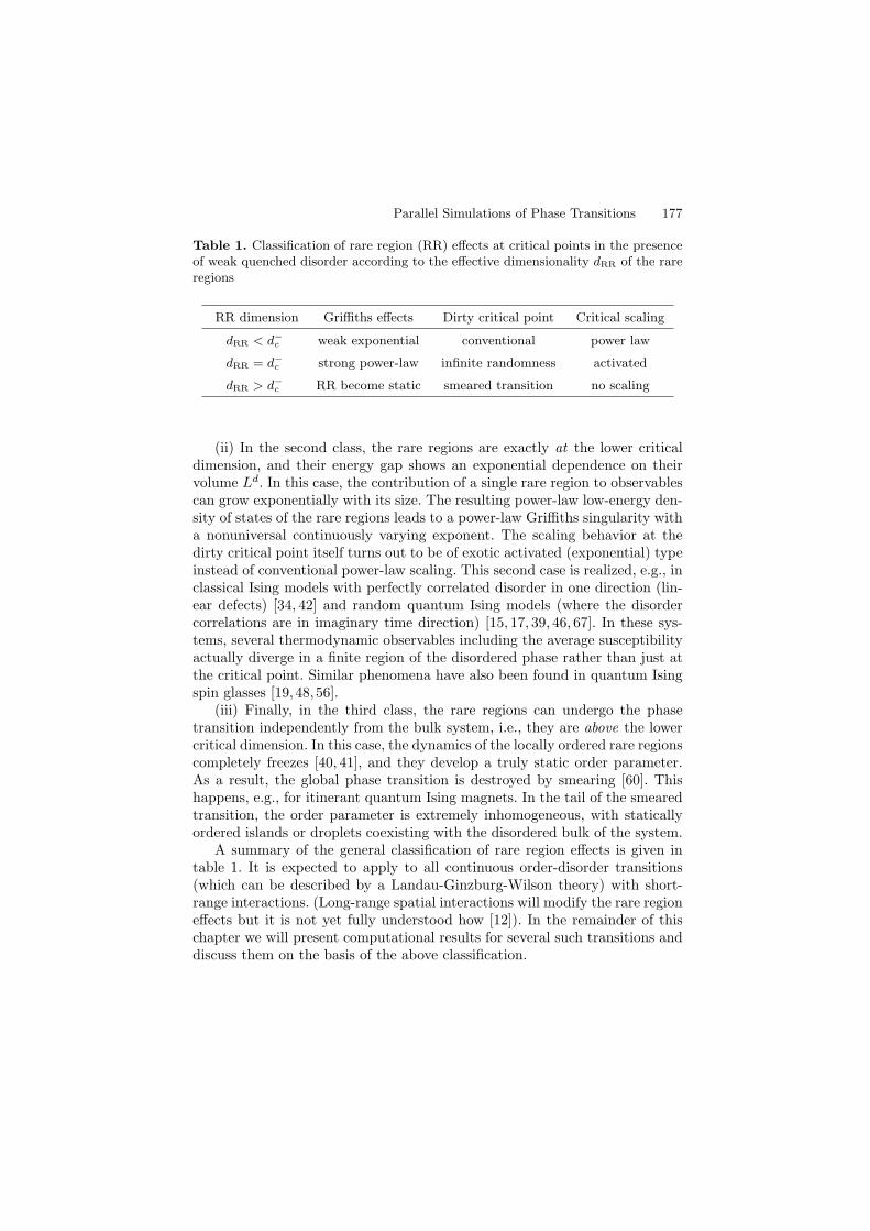
Parallel Simulations of Phase Transitions 177
Table 1. Classification of rare region (RR) effects at critical points in the presenceof weak quenched disorder according to the effective dimensionality dRR of the rareregions
RR dimension Griffiths effects Dirty critical point Critical scaling
dRR < d−c weak exponential conventional power law
dRR = d−c strong power-law infinite randomness activated
dRR > d−c RR become static smeared transition no scaling
(ii) In the second class, the rare regions are exactly at the lower criticaldimension, and their energy gap shows an exponential dependence on theirvolume Ld. In this case, the contribution of a single rare region to observablescan grow exponentially with its size. The resulting power-law low-energy den-sity of states of the rare regions leads to a power-law Griffiths singularity witha nonuniversal continuously varying exponent. The scaling behavior at thedirty critical point itself turns out to be of exotic activated (exponential) typeinstead of conventional power-law scaling. This second case is realized, e.g., inclassical Ising models with perfectly correlated disorder in one direction (lin-ear defects) [34, 42] and random quantum Ising models (where the disordercorrelations are in imaginary time direction) [15, 17, 39, 46, 67]. In these sys-tems, several thermodynamic observables including the average susceptibilityactually diverge in a finite region of the disordered phase rather than just atthe critical point. Similar phenomena have also been found in quantum Isingspin glasses [19,48,56].
(iii) Finally, in the third class, the rare regions can undergo the phasetransition independently from the bulk system, i.e., they are above the lowercritical dimension. In this case, the dynamics of the locally ordered rare regionscompletely freezes [40, 41], and they develop a truly static order parameter.As a result, the global phase transition is destroyed by smearing [60]. Thishappens, e.g., for itinerant quantum Ising magnets. In the tail of the smearedtransition, the order parameter is extremely inhomogeneous, with staticallyordered islands or droplets coexisting with the disordered bulk of the system.
A summary of the general classification of rare region effects is given intable 1. It is expected to apply to all continuous order-disorder transitions(which can be described by a Landau-Ginzburg-Wilson theory) with short-range interactions. (Long-range spatial interactions will modify the rare regioneffects but it is not yet fully understood how [12]). In the remainder of thischapter we will present computational results for several such transitions anddiscuss them on the basis of the above classification.
178 Thomas Vojta
3 Classical Ising magnet with planar defects
3.1 The model
Our first example is a classical equilibrium system, viz. a three-dimensionalclassical Ising magnet. The disorder is perfectly correlated in dC = 2 dimen-sions but uncorrelated in d⊥ = d − dC = 1 dimensions, i.e., the system hasuncorrelated planar defects. The critical behavior of such systems has beeninvestigated in some detail in the literature, but the consistent picture hasbeen slow to emerge. Early renormalization group analysis [33] based on asingle expansion in ǫ = 4 − d did not produce a critical fixed point, leadingto the conclusion that the phase transition is either smeared or of first order.Later work [2] which included an expansion in the number of correlated di-mensions dC lead to a fixed point with conventional power law scaling. Notice,however, that the perturbative renormalization group calculations missed alleffects coming form the rare regions. Recently, a theory based on extremalstatistics arguments [61] has predicted that in this system rare region effectscompletely destroy the sharp phase transition by smearing. The predictionsof this theory were confirmed in simulations of mean-field type models [61].
Here we report results of large-scale Monte-Carlo simulations aimed attesting the theoretical predictions for a realistic model with short-range in-teractions [53]. Our starting point is a three-dimensional Ising model withplanar defects. Classical Ising spins Sijk = ±1 reside on a cubic lattice. Theyinteract via nearest-neighbor interactions. In the clean system all interactionsare identical and have the value J . The defects are modeled via ’weak’ bondsrandomly distributed in one dimension (uncorrelated direction). The bondsin the remaining two dimensions (correlated directions) remain equal to J .The system effectively consists of blocks separated by parallel planes of weakbonds. Thus, d⊥ = 1 and dC = 2. The Hamiltonian of the system is given by:
H = −∑
i=1,...,L⊥j,k=1,...,LC
JiSi,j,kSi+1,j,k
−∑
i=1,...,L⊥j,k=1,...,LC
J(Si,j,kSi,j+1,k + Si,j,kSi,j,k+1), (1)
where L⊥(LC) is the length in the uncorrelated (correlated) direction, i, jand k are integers counting the sites of the cubic lattice, J is the couplingconstant in the correlated directions and Ji is the random coupling constantin the uncorrelated direction. The Ji are drawn from a binary distribution:
Ji =
cJ with probability p
J with probability 1− p(2)
characterized by the concentration p and the relative strength c of the weakbonds (0 < c ≤ 1). The fact that one can independently vary concentration
Parallel Simulations of Phase Transitions 179
and strength of the defects in an easy way is the main advantage of this binarydisorder distribution. The order parameter of the magnetic phase transitionis the total magnetization:
m =1
V
∑
i,j,k
〈Si,j,k〉, (3)
where V = L⊥L2C is the volume of the system, and 〈·〉 is the thermodynamic
average.
3.2 Numerical method
We have performed large scale Monte-Carlo simulations of the Hamiltonian(1) employing the the Wolff cluster algorithm [66]. It can be used becausethe disorder in our system is not frustrated. As discussed above, the expectedsmearing of the transition is a result of exponentially rare events. Thereforesufficiently large system sizes are required in order to observe it. We havesimulated system sizes ranging from L⊥ = 50 to L⊥ = 200 in the uncorrelateddirection and from LC = 50 to LC = 400 in the remaining two correlateddirections, with the largest system simulated having a total of 32 millionspins. We have chosen J = 1 and c = 0.1 in the eq. (2), i.e., the strength ofa ’weak’ bond is 10% of the strength of a strong bond. The simulations havebeen performed for various disorder concentrations p = 0.2, 0.25, 0.3. Thevalues for concentration p and strength c of the weak bonds have been chosenin order to observe the desired behavior over a sufficiently broad interval oftemperatures. The temperature range has been T = 4.325 to T = 4.525,close to the critical temperature of the clean three-dimensional Ising modelT 0
c = 4.511.To achieve optimal performance of the simulations, one must carefully
choose the number NS of disorder realizations (i.e., samples) and the numberNI of measurements during the simulation of each sample. Assuming fullstatistical independence between different measurements (quite possible witha cluster update), the variance σ2
T of the final result (thermodynamically anddisorder averaged) for a particular observable is given by [3]
σ2T = (σ2
S + σ2I/NI)/NS (4)
where σS is the disorder-induced variance between samples and σI is thevariance of measurements within each sample. Since the computational effortis roughly proportional to NINS (neglecting equilibration for the moment), itis then clear that the optimum value of NI is very small. One might even betempted to measure only once per sample. On the other hand, with too shortmeasurement runs most computer time would be spent on equilibration.
In order to balance these requirements we have used a large number NS ofdisorder realizations, ranging from 30 to 780, depending on the system size and
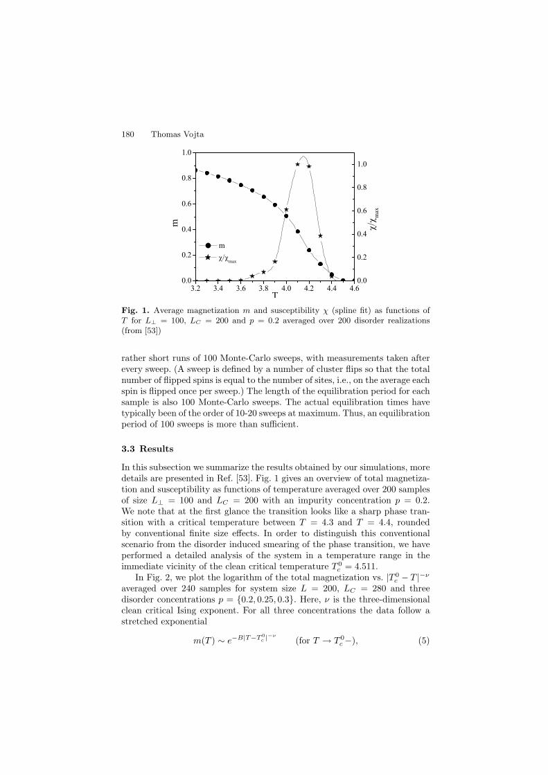
180 Thomas Vojta
Fig. 1. Average magnetization m and susceptibility χ (spline fit) as functions ofT for L⊥ = 100, LC = 200 and p = 0.2 averaged over 200 disorder realizations(from [53])
rather short runs of 100 Monte-Carlo sweeps, with measurements taken afterevery sweep. (A sweep is defined by a number of cluster flips so that the totalnumber of flipped spins is equal to the number of sites, i.e., on the average eachspin is flipped once per sweep.) The length of the equilibration period for eachsample is also 100 Monte-Carlo sweeps. The actual equilibration times havetypically been of the order of 10-20 sweeps at maximum. Thus, an equilibrationperiod of 100 sweeps is more than sufficient.
3.3 Results
In this subsection we summarize the results obtained by our simulations, moredetails are presented in Ref. [53]. Fig. 1 gives an overview of total magnetiza-tion and susceptibility as functions of temperature averaged over 200 samplesof size L⊥ = 100 and LC = 200 with an impurity concentration p = 0.2.We note that at the first glance the transition looks like a sharp phase tran-sition with a critical temperature between T = 4.3 and T = 4.4, roundedby conventional finite size effects. In order to distinguish this conventionalscenario from the disorder induced smearing of the phase transition, we haveperformed a detailed analysis of the system in a temperature range in theimmediate vicinity of the clean critical temperature T 0
c = 4.511.In Fig. 2, we plot the logarithm of the total magnetization vs. |T 0
c − T |−ν
averaged over 240 samples for system size L = 200, LC = 280 and threedisorder concentrations p = 0.2, 0.25, 0.3. Here, ν is the three-dimensionalclean critical Ising exponent. For all three concentrations the data follow astretched exponential
m(T ) ∼ e−B|T−T 0c |−ν
(for T → T 0c−), (5)
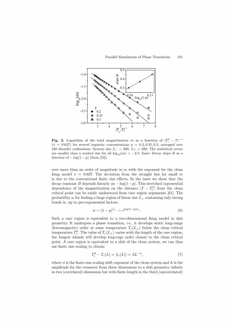
Parallel Simulations of Phase Transitions 181
Fig. 2. Logarithm of the total magnetization m as a function of |T 0c − T |−ν
(ν = 0.627) for several impurity concentrations p = 0.2, 0.25, 0.3, averaged over240 disorder realizations. System size L⊥ = 200, LC = 280. The statistical errorsare smaller than a symbol size for all log10(m) > −2.5. Inset: Decay slope B as afunction of − log(1 − p) (from [53])
over more than an order of magnitude in m with the exponent for the cleanIsing model ν = 0.627. The deviation from the straight line for small mis due to the conventional finite size effects. In the inset we show that thedecay constant B depends linearly on − log(1−p). This stretched exponentialdependence of the magnetization on the distance |T − T 0
c | from the cleancritical point can be easily understood from rare region arguments [61]. Theprobability w for finding a large region of linear size L⊥ containing only strongbonds is, up to pre-exponential factors:
w ∼ (1− p)L⊥ = elog(1−p)L⊥ . (6)
Such a rare region is equivalent to a two-dimensional Ising model in slabgeometry. It undergoes a phase transition, i.e., it develops static long-range(ferromagnetic) order at some temperature Tc(L⊥) below the clean criticaltemperature T 0
c . The value of Tc(L⊥) varies with the length of the rare region;the longest islands will develop long-rage order closest to the clean criticalpoint. A rare region is equivalent to a slab of the clean system, we can thususe finite size scaling to obtain:
T 0c − Tc(L) = |tc(L)| = AL−φ, (7)
where φ is the finite-size scaling shift exponent of the clean system and A is theamplitude for the crossover from three dimensions to a slab geometry infinitein two (correlated) dimension but with finite length in the third (uncorrelated)
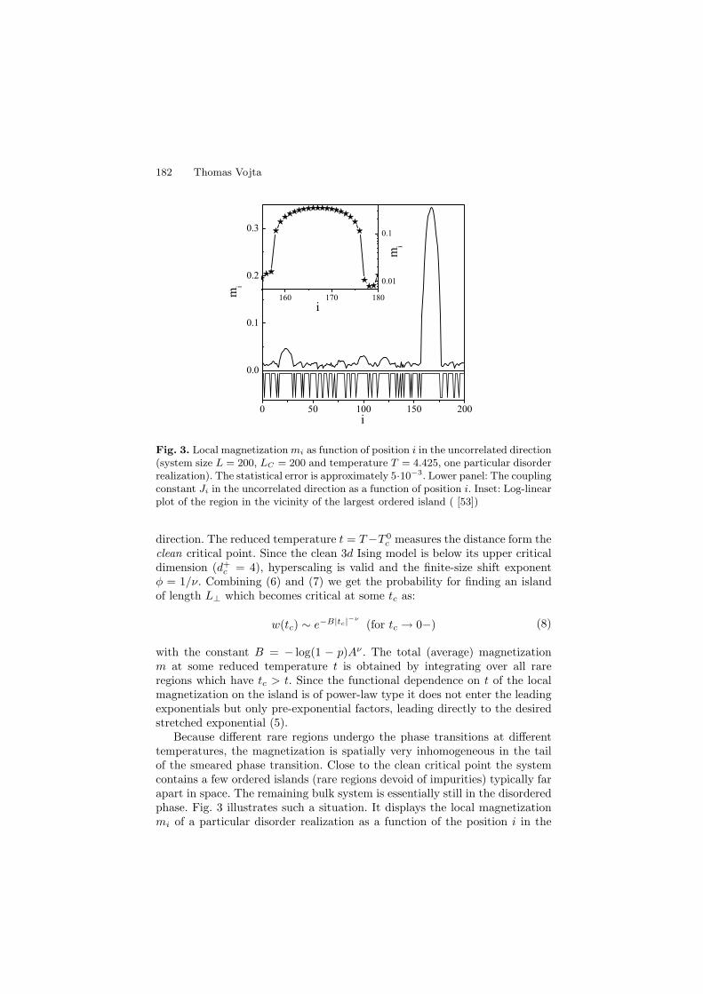
182 Thomas Vojta
Fig. 3. Local magnetization mi as function of position i in the uncorrelated direction(system size L = 200, LC = 200 and temperature T = 4.425, one particular disorderrealization). The statistical error is approximately 5·10−3. Lower panel: The couplingconstant Ji in the uncorrelated direction as a function of position i. Inset: Log-linearplot of the region in the vicinity of the largest ordered island ( [53])
direction. The reduced temperature t = T−T 0c measures the distance form the
clean critical point. Since the clean 3d Ising model is below its upper criticaldimension (d+c = 4), hyperscaling is valid and the finite-size shift exponentφ = 1/ν. Combining (6) and (7) we get the probability for finding an islandof length L⊥ which becomes critical at some tc as:
w(tc) ∼ e−B|tc|−ν
(for tc → 0−) (8)
with the constant B = − log(1 − p)Aν . The total (average) magnetizationm at some reduced temperature t is obtained by integrating over all rareregions which have tc > t. Since the functional dependence on t of the localmagnetization on the island is of power-law type it does not enter the leadingexponentials but only pre-exponential factors, leading directly to the desiredstretched exponential (5).
Because different rare regions undergo the phase transitions at differenttemperatures, the magnetization is spatially very inhomogeneous in the tailof the smeared phase transition. Close to the clean critical point the systemcontains a few ordered islands (rare regions devoid of impurities) typically farapart in space. The remaining bulk system is essentially still in the disorderedphase. Fig. 3 illustrates such a situation. It displays the local magnetizationmi of a particular disorder realization as a function of the position i in the
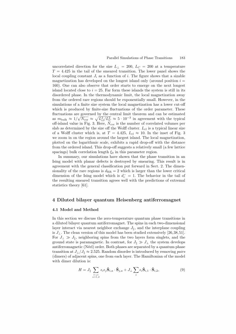
Parallel Simulations of Phase Transitions 183
uncorrelated direction for the size L⊥ = 200, LC = 200 at a temperatureT = 4.425 in the tail of the smeared transition. The lower panel shows thelocal coupling constant Ji as a function of i. The figure shows that a sizablemagnetization has developed on the longest island only (around position i =160). One can also observe that order starts to emerge on the next longestisland located close to i = 25. Far form these islands the system is still in itsdisordered phase. In the thermodynamic limit, the local magnetization awayfrom the ordered rare regions should be exponentially small. However, in thesimulations of a finite size system the local magnetization has a lower cut-offwhich is produced by finite-size fluctuations of the order parameter. Thesefluctuations are governed by the central limit theorem and can be estimatedas mbulk ≈ 1/
√Ncor ≈
√L2
cl/L2C ≈ 5 · 10−3 in agreement with the typical
off-island value in Fig. 3. Here, Ncor is the number of correlated volumes perslab as determined by the size off the Wolff cluster. Lcl is a typical linear sizeof a Wolff cluster which is, at T = 4.425, Lcl ≈ 10. In the inset of Fig. 3we zoom in on the region around the largest island. The local magnetization,plotted on the logarithmic scale, exhibits a rapid drop-off with the distancefrom the ordered island. This drop-off suggests a relatively small (a few latticespacings) bulk correlation length ξ0 in this parameter region.
In summary, our simulations have shown that the phase transition in anIsing model with planar defects is destroyed by smearing. This result is inagreement with the general classification put forward in Sect. 2. The dimen-sionality of the rare regions is dRR = 2 which is larger than the lower criticaldimension of the Ising model which is d−c = 1. The behavior in the tail ofthe resulting smeared transition agrees well with the predictions of extremalstatistics theory [61].
4 Diluted bilayer quantum Heisenberg antiferromagnet
4.1 Model and Method
In this section we discuss the zero-temperature quantum phase transitions ina diluted bilayer quantum antiferromagnet. The spins in each two-dimensionallayer interact via nearest neighbor exchange J‖, and the interplane couplingis J⊥. The clean version of this model has been studied extensively [26,38,51].For J⊥ ≫ J‖, neighboring spins from the two layers form singlets, and theground state is paramagnetic. In contrast, for J‖ ≫ J⊥ the system developsantiferromagnetic (Neel) order. Both phases are separated by a quantum phasetransition at J⊥/J‖ ≈ 2.525. Random disorder is introduced by removing pairs(dimers) of adjacent spins, one from each layer. The Hamiltonian of the modelwith dimer dilution is:
H = J‖∑
〈i,j〉a=1,2
ǫiǫjSi,a · Sj,a + J⊥∑
i
ǫiSi,1 · Si,2, (9)
184 Thomas Vojta
0 0.1 0.2 0.3 0.4
p
0
0.5
1
1.5
2
2.5
J ⊥ /
J||
AF ordered
disordered
J
J
Fig. 4. Phase diagram [59] of the diluted bilayer Heisenberg antiferromagnet, asfunction of J⊥/J‖ and dilution p. The dashed line is the percolation threshold, theopen dot is the multicritical point of Refs. [50, 59]. The arrow indicates the QPTstudied here. Inset: The model: Quantum spins (arrows) reside on the two parallelsquare lattices. The spins in each plane interact with the coupling strength J‖.Interplane coupling is J⊥. Dilution is done by removing dimers (from [54])
and ǫi=0 (ǫi=1) with probability p (1− p).The phase diagram of the dimer-diluted bilayer Heisenberg model has been
studied by Sandvik [50] and Vajk and Greven [59], see Fig. 4. For small J⊥,magnetic order survives up to the percolation threshold pp ≈ 0.4072, and amulticritical point exists at p = pp and J⊥/J‖ ≈ 0.16.
We have performed extensive simulations [54] of the critical behavior at thegeneric transition occurring for 0 < p < pp and driven by J⊥. To this end wehave first mapped the quantum Hamiltonian (9) onto a classical model. Thelow-energy properties of bilayer quantum antiferromagnets are represented bya (2+1)-dimensional O(3) quantum rotor model [10] with the rotor coordinateni corresponding to Si,1 − Si,2 and the angular momentum Li representing
Si,1 + Si,2 (see, e.g., Chap. 5 of [49]). This quantum rotor model in turn isequivalent to a three-dimensional classical Heisenberg model with the disorderperfectly correlated in imaginary time direction, as can be easily seen froma path integral representation of the partition function. Thus, our classicalHamiltonian reads:
H = K∑
〈i,j〉,τ
ǫiǫjni,τ · nj,τ +K∑
i,τ
ǫini,τ · ni,τ+1, (10)
where ni,τ is an O(3) unit vector. The coupling constant βK of the classicalmodel is related to the ratio J‖/J⊥ of the quantum model. Here, β ≡ 1/Twhere T is an effective “classical” temperature, not equal to the real temper-ature which is zero. We set K = 1 and drive the classical system through thetransition by tuning the classical temperature T .
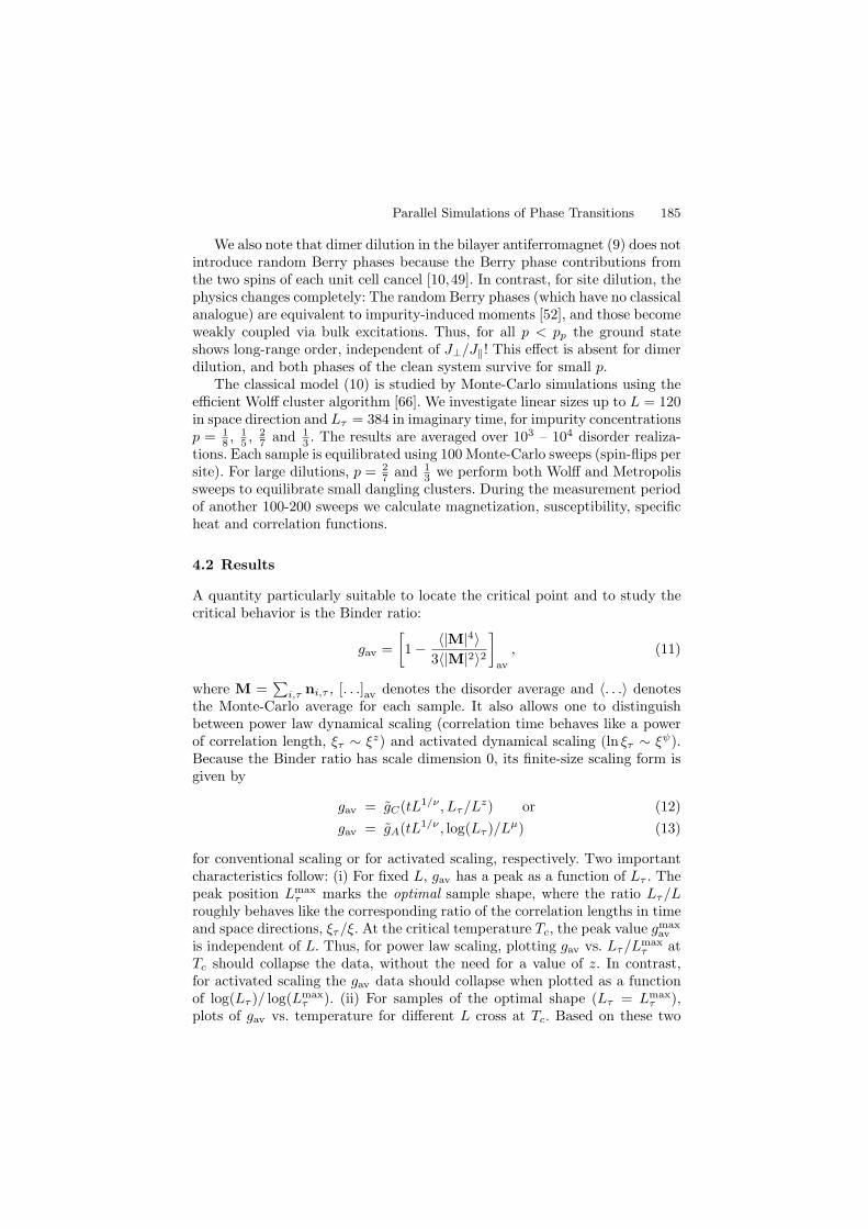
Parallel Simulations of Phase Transitions 185
We also note that dimer dilution in the bilayer antiferromagnet (9) does notintroduce random Berry phases because the Berry phase contributions fromthe two spins of each unit cell cancel [10,49]. In contrast, for site dilution, thephysics changes completely: The random Berry phases (which have no classicalanalogue) are equivalent to impurity-induced moments [52], and those becomeweakly coupled via bulk excitations. Thus, for all p < pp the ground stateshows long-range order, independent of J⊥/J‖! This effect is absent for dimerdilution, and both phases of the clean system survive for small p.
The classical model (10) is studied by Monte-Carlo simulations using theefficient Wolff cluster algorithm [66]. We investigate linear sizes up to L = 120in space direction and Lτ = 384 in imaginary time, for impurity concentrationsp = 1
8 , 15 , 2
7 and 13 . The results are averaged over 103 – 104 disorder realiza-
tions. Each sample is equilibrated using 100 Monte-Carlo sweeps (spin-flips persite). For large dilutions, p = 2
7 and 13 we perform both Wolff and Metropolis
sweeps to equilibrate small dangling clusters. During the measurement periodof another 100-200 sweeps we calculate magnetization, susceptibility, specificheat and correlation functions.
4.2 Results
A quantity particularly suitable to locate the critical point and to study thecritical behavior is the Binder ratio:
gav =
[1− 〈|M|4〉
3〈|M|2〉2]
av
, (11)
where M =∑
i,τ ni,τ , [. . .]av denotes the disorder average and 〈. . .〉 denotesthe Monte-Carlo average for each sample. It also allows one to distinguishbetween power law dynamical scaling (correlation time behaves like a powerof correlation length, ξτ ∼ ξz) and activated dynamical scaling (ln ξτ ∼ ξψ).Because the Binder ratio has scale dimension 0, its finite-size scaling form isgiven by
gav = gC(tL1/ν , Lτ/Lz) or (12)
gav = gA(tL1/ν , log(Lτ )/Lµ) (13)
for conventional scaling or for activated scaling, respectively. Two importantcharacteristics follow: (i) For fixed L, gav has a peak as a function of Lτ . Thepeak position Lmax
τ marks the optimal sample shape, where the ratio Lτ/Lroughly behaves like the corresponding ratio of the correlation lengths in timeand space directions, ξτ/ξ. At the critical temperature Tc, the peak value gmax
av
is independent of L. Thus, for power law scaling, plotting gav vs. Lτ/Lmaxτ at
Tc should collapse the data, without the need for a value of z. In contrast,for activated scaling the gav data should collapse when plotted as a functionof log(Lτ )/ log(Lmax
τ ). (ii) For samples of the optimal shape (Lτ = Lmaxτ ),
plots of gav vs. temperature for different L cross at Tc. Based on these two
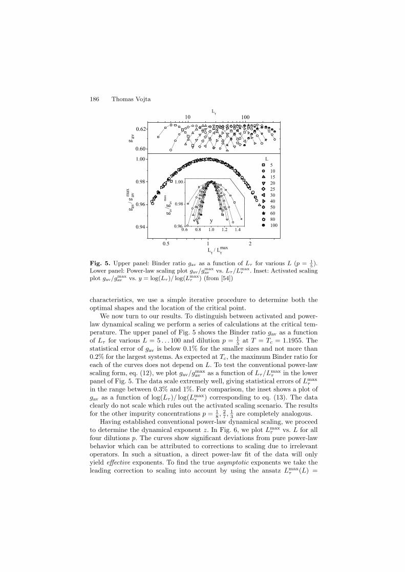
186 Thomas Vojta
2
Fig. 5. Upper panel: Binder ratio gav as a function of Lτ for various L (p = 15).
Lower panel: Power-law scaling plot gav/gmaxav vs. Lτ/Lmax
τ . Inset: Activated scalingplot gav/gmax
av vs. y = log(Lτ )/ log(Lmaxτ ) (from [54])
characteristics, we use a simple iterative procedure to determine both theoptimal shapes and the location of the critical point.
We now turn to our results. To distinguish between activated and power-law dynamical scaling we perform a series of calculations at the critical tem-perature. The upper panel of Fig. 5 shows the Binder ratio gav as a functionof Lτ for various L = 5 . . . 100 and dilution p = 1
5 at T = Tc = 1.1955. Thestatistical error of gav is below 0.1% for the smaller sizes and not more than0.2% for the largest systems. As expected at Tc, the maximum Binder ratio foreach of the curves does not depend on L. To test the conventional power-lawscaling form, eq. (12), we plot gav/g
maxav as a function of Lτ/L
maxτ in the lower
panel of Fig. 5. The data scale extremely well, giving statistical errors of Lmaxτ
in the range between 0.3% and 1%. For comparison, the inset shows a plot ofgav as a function of log(Lτ )/ log(Lmax
τ ) corresponding to eq. (13). The dataclearly do not scale which rules out the activated scaling scenario. The resultsfor the other impurity concentrations p = 1
8 ,27 ,
13 are completely analogous.
Having established conventional power-law dynamical scaling, we proceedto determine the dynamical exponent z. In Fig. 6, we plot Lmax
τ vs. L for allfour dilutions p. The curves show significant deviations from pure power-lawbehavior which can be attributed to corrections to scaling due to irrelevantoperators. In such a situation, a direct power-law fit of the data will onlyyield effective exponents. To find the true asymptotic exponents we take theleading correction to scaling into account by using the ansatz Lmax
τ (L) =
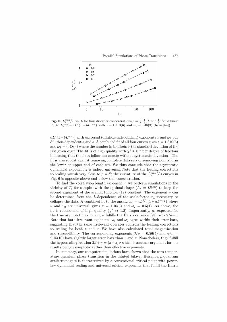
Parallel Simulations of Phase Transitions 187
Fig. 6. Lmaxτ /L vs. L for four disorder concentrations p = 1
8, 1
5, 2
7and 1
3. Solid lines:
Fit to Lmaxτ = aLz(1 + bL−ω1) with z = 1.310(6) and ω1 = 0.48(3) (from [54])
aLz(1+bL−ω1) with universal (dilution-independent) exponents z and ω1 butdilution-dependent a and b. A combined fit of all four curves gives z = 1.310(6)and ω1 = 0.48(3) where the number in brackets is the standard deviation of thelast given digit. The fit is of high quality with χ2 ≈ 0.7 per degree of freedomindicating that the data follow our ansatz without systematic deviations. Thefit is also robust against removing complete data sets or removing points formthe lower or upper end of each set. We thus conclude that the asymptoticdynamical exponent z is indeed universal. Note that the leading correctionsto scaling vanish very close to p = 2
7 ; the curvature of the Lmaxτ (L) curves in
Fig. 6 is opposite above and below this concentration.To find the correlation length exponent ν, we perform simulations in the
vicinity of Tc for samples with the optimal shape (Lτ = Lmaxτ ) to keep the
second argument of the scaling function (12) constant. The exponent ν canbe determined from the L-dependence of the scale-factor xL necessary tocollapse the data. A combined fit to the ansatz xL = cL1/ν(1 + dL−ω2) whereν and ω2 are universal, gives ν = 1.16(3) and ω2 = 0.5(1). As above, thefit is robust and of high quality (χ2 ≈ 1.2). Importantly, as expected forthe true asymptotic exponent, ν fulfills the Harris criterion [24], ν > 2/d=1.Note that both irrelevant exponents ω1 and ω2 agree within their error bars,suggesting that the same irrelevant operator controls the leading correctionsto scaling for both z and ν. We have also calculated total magnetizationand susceptibility. The corresponding exponents β/ν = 0.56(5) and γ/ν =2.15(10) have slightly larger error bars than z and ν. Nonetheless, they fulfillthe hyperscaling relation 2β+γ = (d+ z)ν which is another argument for ourresults being asymptotic rather than effective exponents.
In summary, our computer simulations have shown that the zero-temper-ature quantum phase transition in the diluted bilayer Heisenberg quantumantiferromagnet is characterized by a conventional critical point with power-law dynamical scaling and universal critical exponents that fulfill the Harris
188 Thomas Vojta
criterion. These results are in agreement with the general classification sug-gested in Sect. 2. The effective dimensionality of the rare regions (includingthe imaginary time direction which is important for quantum phase transi-tions) is dRR = 1. The lower critical dimension for an O(3) Heisenberg modelis d−c = 2. Thus, dRR < d
−c , and the rare region effects are exponentially small.
5 Nonequilibrium phase transitions in the disorderedcontact process
5.1 The contact process
The examples discussed in Sects. 3 and 4 concerned systems in thermal equilib-rium. However, nonequilibrium systems can also undergo “phase” transitionsbetween different nonequilibrium steady states. These transitions are charac-terized by large scale fluctuations and collective behavior over large distancesand times very similar to the behavior at equilibrium critical points. Exam-ples of such nonequilibrium transitions can be found in population dynamicsand epidemics, chemical reactions, growing surfaces, and in granular flow andtraffic jams (for recent reviews see, e.g., Refs. [9, 27,35,44,55,57])
A prominent class of nonequilibrium phase transitions separates activefluctuating states from inactive, absorbing states where fluctuations cease en-tirely. Recently, much effort has been devoted to classifying possible univer-sality classes of these absorbing state phase transitions [27, 44]. The genericuniversality class is directed percolation (DP) [23]. According to a conjectureby Janssen and Grassberger [20, 30], all absorbing state transitions with ascalar order parameter, short-range interactions, and no extra symmetries orconservation laws belong to this class.
The contact process [25] is a prototypical system in the directed percolationuniversality class. It can be interpreted, e.g., as a model for the spreading of adisease. The contact process is defined on a d-dimensional hypercubic lattice.Each lattice site r can be active (occupied by a particle) or inactive (empty).In the course of the time evolution, active sites can infect their neighbors, orthey can spontaneously become inactive. Specifically, the dynamics is given bya continuous-time Markov process during which particles are created at emptysites at a rate λn/(2d) where n is the number of active nearest neighbor sites.Particles are annihilated at rate µ (which is often set to unity without loss ofgenerality). The ratio of the two rates controls the behavior of the system.
For small birth rate λ, annihilation dominates, and the absorbing statewithout any particles is the only steady state (inactive phase). For large birthrate λ, there is a steady state with nonzero particle density (active phase).The two phases are separated by a nonequilibrium phase transition in thedirected percolation universality class at λ = λ0
c . The central quantity in thecontact process is the average density of active sites at time t
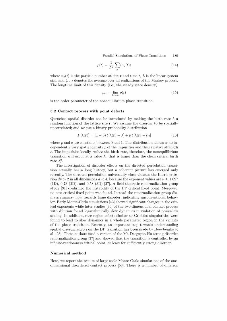
Parallel Simulations of Phase Transitions 189
ρ(t) =1
Ld
∑
r
〈nr(t)〉 (14)
where nr(t) is the particle number at site r and time t, L is the linear systemsize, and 〈. . .〉 denotes the average over all realizations of the Markov process.The longtime limit of this density (i.e., the steady state density)
ρst = limt→∞
ρ(t) (15)
is the order parameter of the nonequilibrium phase transition.
5.2 Contact process with point defects
Quenched spatial disorder can be introduced by making the birth rate λ arandom function of the lattice site r. We assume the disorder to be spatiallyuncorrelated; and we use a binary probability distribution
P [λ(r)] = (1− p) δ[λ(r)− λ] + p δ[λ(r)− cλ] (16)
where p and c are constants between 0 and 1. This distribution allows us to in-dependently vary spatial density p of the impurities and their relative strengthc. The impurities locally reduce the birth rate, therefore, the nonequilibriumtransition will occur at a value λc that is larger than the clean critical birthrate λ0
c .The investigation of disorder effects on the directed percolation transi-
tion actually has a long history, but a coherent picture has emerged onlyrecently. The directed percolation universality class violates the Harris crite-rion dν > 2 in all dimensions d < 4, because the exponent values are ν ≈ 1.097(1D), 0.73 (2D), and 0.58 (3D) [27]. A field-theoretic renormalization groupstudy [31] confirmed the instability of the DP critical fixed point. Moreover,no new critical fixed point was found. Instead the renormalization group dis-plays runaway flow towards large disorder, indicating unconventional behav-ior. Early Monte-Carlo simulations [43] showed significant changes in the crit-ical exponents while later studies [36] of the two-dimensional contact processwith dilution found logarithmically slow dynamics in violation of power-lawscaling. In addition, rare region effects similar to Griffiths singularities werefound to lead to slow dynamics in a whole parameter region in the vicinityof the phase transition. Recently, an important step towards understandingspatial disorder effects on the DP transition has been made by Hooyberghs etal. [28]. These authors used a version of the Ma-Dasgupta-Hu strong-disorderrenormalization group [37] and showed that the transition is controlled by aninfinite-randomness critical point, at least for sufficiently strong disorder.
Numerical method
Here, we report the results of large scale Monte-Carlo simulations of the one-dimensional disordered contact process [58]. There is a number of different
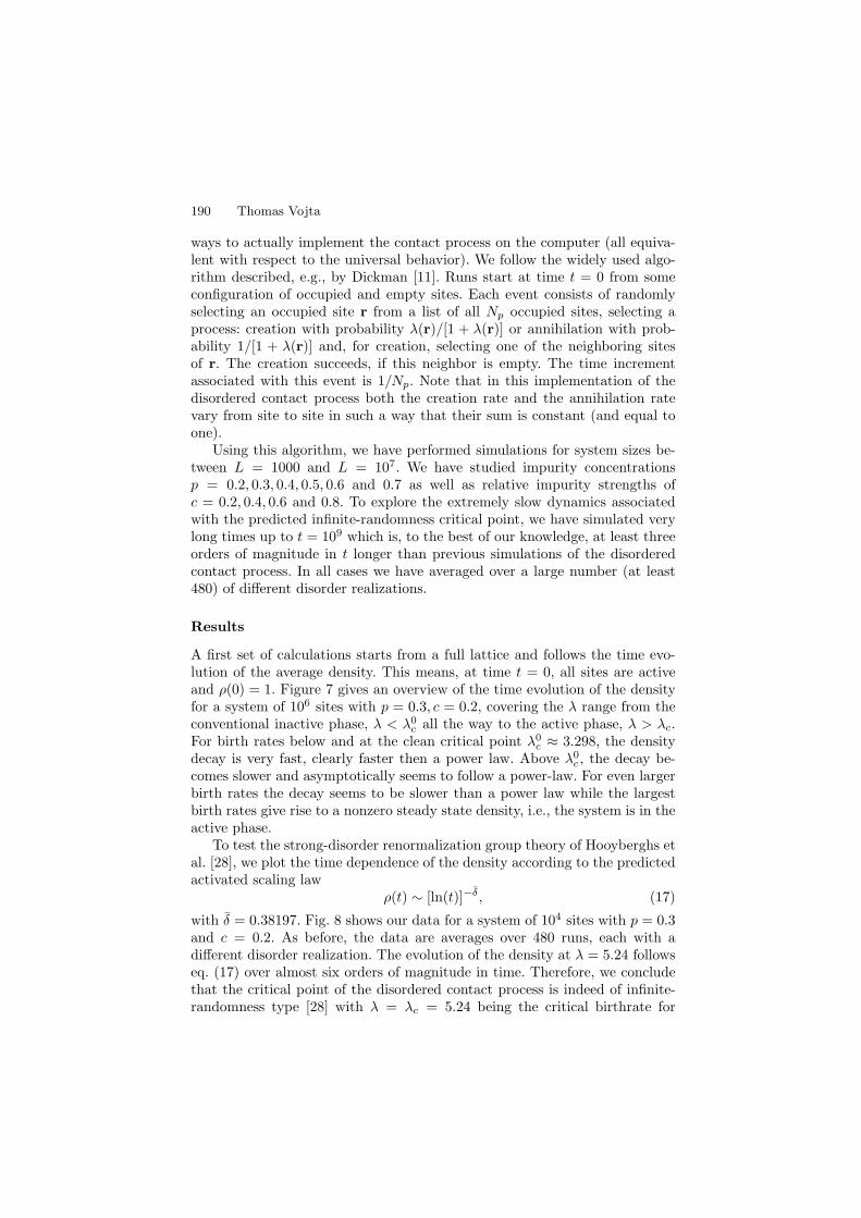
190 Thomas Vojta
ways to actually implement the contact process on the computer (all equiva-lent with respect to the universal behavior). We follow the widely used algo-rithm described, e.g., by Dickman [11]. Runs start at time t = 0 from someconfiguration of occupied and empty sites. Each event consists of randomlyselecting an occupied site r from a list of all Np occupied sites, selecting aprocess: creation with probability λ(r)/[1 + λ(r)] or annihilation with prob-ability 1/[1 + λ(r)] and, for creation, selecting one of the neighboring sitesof r. The creation succeeds, if this neighbor is empty. The time incrementassociated with this event is 1/Np. Note that in this implementation of thedisordered contact process both the creation rate and the annihilation ratevary from site to site in such a way that their sum is constant (and equal toone).
Using this algorithm, we have performed simulations for system sizes be-tween L = 1000 and L = 107. We have studied impurity concentrationsp = 0.2, 0.3, 0.4, 0.5, 0.6 and 0.7 as well as relative impurity strengths ofc = 0.2, 0.4, 0.6 and 0.8. To explore the extremely slow dynamics associatedwith the predicted infinite-randomness critical point, we have simulated verylong times up to t = 109 which is, to the best of our knowledge, at least threeorders of magnitude in t longer than previous simulations of the disorderedcontact process. In all cases we have averaged over a large number (at least480) of different disorder realizations.
Results
A first set of calculations starts from a full lattice and follows the time evo-lution of the average density. This means, at time t = 0, all sites are activeand ρ(0) = 1. Figure 7 gives an overview of the time evolution of the densityfor a system of 106 sites with p = 0.3, c = 0.2, covering the λ range from theconventional inactive phase, λ < λ0
c all the way to the active phase, λ > λc.For birth rates below and at the clean critical point λ0
c ≈ 3.298, the densitydecay is very fast, clearly faster then a power law. Above λ0
c , the decay be-comes slower and asymptotically seems to follow a power-law. For even largerbirth rates the decay seems to be slower than a power law while the largestbirth rates give rise to a nonzero steady state density, i.e., the system is in theactive phase.
To test the strong-disorder renormalization group theory of Hooyberghs etal. [28], we plot the time dependence of the density according to the predictedactivated scaling law
ρ(t) ∼ [ln(t)]−δ, (17)
with δ = 0.38197. Fig. 8 shows our data for a system of 104 sites with p = 0.3and c = 0.2. As before, the data are averages over 480 runs, each with adifferent disorder realization. The evolution of the density at λ = 5.24 followseq. (17) over almost six orders of magnitude in time. Therefore, we concludethat the critical point of the disordered contact process is indeed of infinite-randomness type [28] with λ = λc = 5.24 being the critical birthrate for
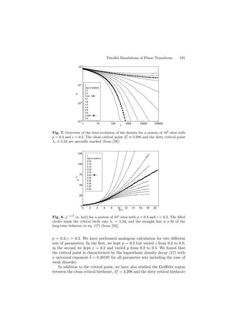
Parallel Simulations of Phase Transitions 191
1 10 100 1000 10000 100000t
10-3
10-2
10-1
100
ρ
λ
(top to bottom)
5.7
5.4
5.24
5.1
4.8
4.5
4.2
3.9
3.6
3.298
2.9
Fig. 7. Overview of the time evolution of the density for a system of 106 sites withp = 0.3 and c = 0.2. The clean critical point λ0
c ≈ 3.298 and the dirty critical pointλc ≈ 5.24 are specially marked (from [58])
0 2 4 6 8 10 12 14 16 18 20ln t
0
25
50
75
100
125
ρ−
1/δ
λ
(top to bottom)
5.00
5.10
5.15
5.20
5.22
5.24
5.26
5.28
5.30
5.32
5.35
Fig. 8. ρ−1/δ vs. ln(t) for a system of 104 sites with p = 0.3 and c = 0.2. The filledcircles mark the critical birth rate λc = 5.24, and the straight line is a fit of thelong-time behavior to eq. (17) (from [58])
p = 0.3, c = 0.2. We have performed analogous calculation for two differentsets of parameters. In the first, we kept p = 0.3 but varied c from 0.2 to 0.8;in the second we kept c = 0.2 and varied p from 0.2 to 0.5. We found thatthe critical point is characterized by the logarithmic density decay (17) witha universal exponent δ = 0.38197 for all parameter sets including the case ofweak disorder.
In addition to the critical point, we have also studied the Griffiths regionbetween the clean critical birthrate, λ0
c = 3.298 and the dirty critical birthrate
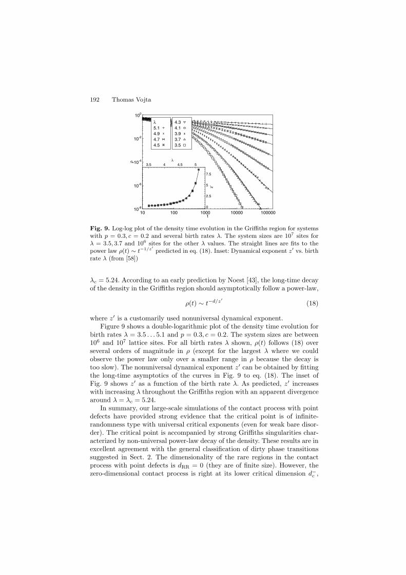
192 Thomas Vojta
10 100 1000 10000 100000t
10-8
10-6
10-4
10-2
100
ρ
4.3
4.1
3.9
3.7
3.5
λ
5.1
4.9
4.7
4.5
3.5 4 4.5 5λ
0
2.5
5
7.5
z’
Fig. 9. Log-log plot of the density time evolution in the Griffiths region for systemswith p = 0.3, c = 0.2 and several birth rates λ. The system sizes are 107 sites forλ = 3.5, 3.7 and 106 sites for the other λ values. The straight lines are fits to thepower law ρ(t) ∼ t−1/z′
predicted in eq. (18). Inset: Dynamical exponent z′ vs. birthrate λ (from [58])
λc = 5.24. According to an early prediction by Noest [43], the long-time decayof the density in the Griffiths region should asymptotically follow a power-law,
ρ(t) ∼ t−d/z′
(18)
where z′ is a customarily used nonuniversal dynamical exponent.Figure 9 shows a double-logarithmic plot of the density time evolution for
birth rates λ = 3.5 . . . 5.1 and p = 0.3, c = 0.2. The system sizes are between106 and 107 lattice sites. For all birth rates λ shown, ρ(t) follows (18) overseveral orders of magnitude in ρ (except for the largest λ where we couldobserve the power law only over a smaller range in ρ because the decay istoo slow). The nonuniversal dynamical exponent z′ can be obtained by fittingthe long-time asymptotics of the curves in Fig. 9 to eq. (18). The inset ofFig. 9 shows z′ as a function of the birth rate λ. As predicted, z′ increaseswith increasing λ throughout the Griffiths region with an apparent divergencearound λ = λc = 5.24.
In summary, our large-scale simulations of the contact process with pointdefects have provided strong evidence that the critical point is of infinite-randomness type with universal critical exponents (even for weak bare disor-der). The critical point is accompanied by strong Griffiths singularities char-acterized by non-universal power-law decay of the density. These results are inexcellent agreement with the general classification of dirty phase transitionssuggested in Sect. 2. The dimensionality of the rare regions in the contactprocess with point defects is dRR = 0 (they are of finite size). However, thezero-dimensional contact process is right at its lower critical dimension d−c ,
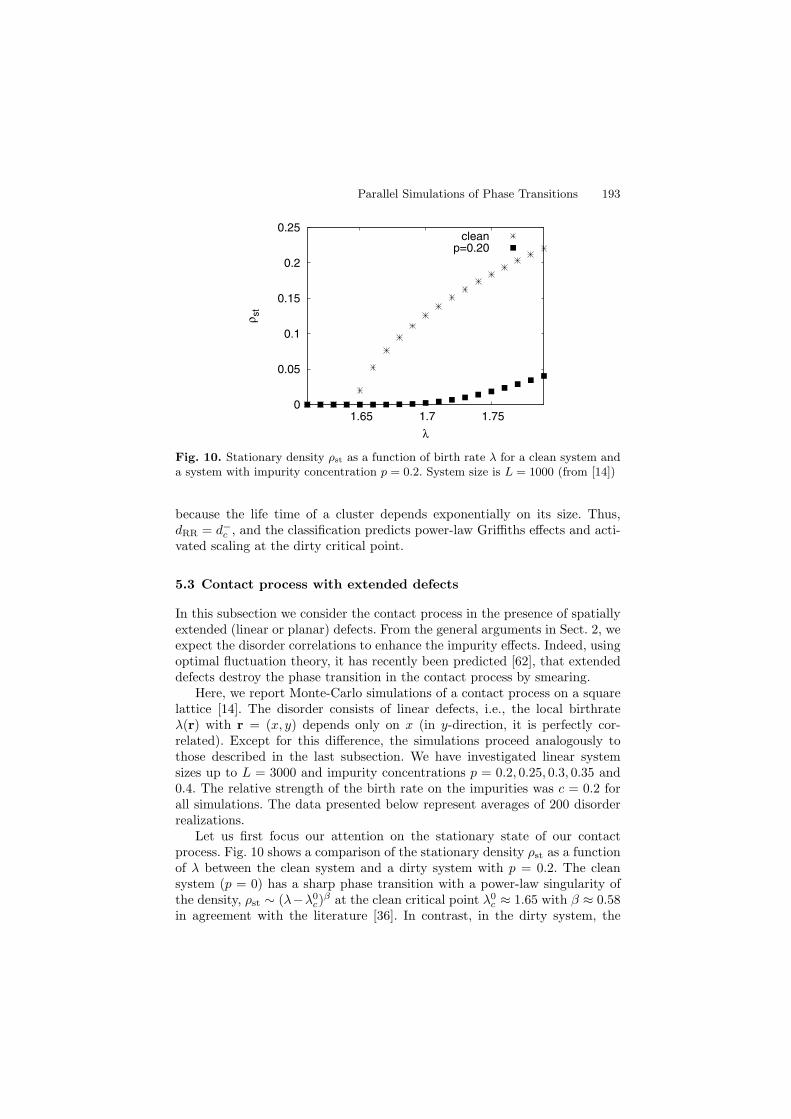
Parallel Simulations of Phase Transitions 193
0
0.05
0.1
0.15
0.2
0.25
1.65 1.7 1.75
ρst
λ
cleanp=0.20
Fig. 10. Stationary density ρst as a function of birth rate λ for a clean system anda system with impurity concentration p = 0.2. System size is L = 1000 (from [14])
because the life time of a cluster depends exponentially on its size. Thus,dRR = d−c , and the classification predicts power-law Griffiths effects and acti-vated scaling at the dirty critical point.
5.3 Contact process with extended defects
In this subsection we consider the contact process in the presence of spatiallyextended (linear or planar) defects. From the general arguments in Sect. 2, weexpect the disorder correlations to enhance the impurity effects. Indeed, usingoptimal fluctuation theory, it has recently been predicted [62], that extendeddefects destroy the phase transition in the contact process by smearing.
Here, we report Monte-Carlo simulations of a contact process on a squarelattice [14]. The disorder consists of linear defects, i.e., the local birthrateλ(r) with r = (x, y) depends only on x (in y-direction, it is perfectly cor-related). Except for this difference, the simulations proceed analogously tothose described in the last subsection. We have investigated linear systemsizes up to L = 3000 and impurity concentrations p = 0.2, 0.25, 0.3, 0.35 and0.4. The relative strength of the birth rate on the impurities was c = 0.2 forall simulations. The data presented below represent averages of 200 disorderrealizations.
Let us first focus our attention on the stationary state of our contactprocess. Fig. 10 shows a comparison of the stationary density ρst as a functionof λ between the clean system and a dirty system with p = 0.2. The cleansystem (p = 0) has a sharp phase transition with a power-law singularity ofthe density, ρst ∼ (λ−λ0
c)β at the clean critical point λ0
c ≈ 1.65 with β ≈ 0.58in agreement with the literature [36]. In contrast, in the dirty system, the
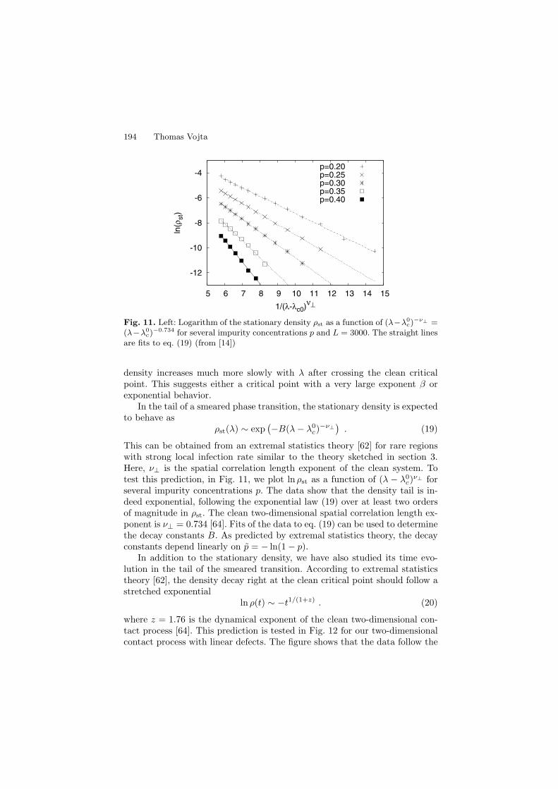
194 Thomas Vojta
-12
-10
-8
-6
-4
5 6 7 8 9 10 11 12 13 14 15
ln(ρ
st)
1/(λ-λc0)ν⊥
p=0.20p=0.25p=0.30p=0.35p=0.40
Fig. 11. Left: Logarithm of the stationary density ρst as a function of (λ−λ0c)
−ν⊥ =(λ−λ0
c)−0.734 for several impurity concentrations p and L = 3000. The straight lines
are fits to eq. (19) (from [14])
density increases much more slowly with λ after crossing the clean criticalpoint. This suggests either a critical point with a very large exponent β orexponential behavior.
In the tail of a smeared phase transition, the stationary density is expectedto behave as
ρst(λ) ∼ exp(−B(λ− λ0
c)−ν⊥
). (19)
This can be obtained from an extremal statistics theory [62] for rare regionswith strong local infection rate similar to the theory sketched in section 3.Here, ν⊥ is the spatial correlation length exponent of the clean system. Totest this prediction, in Fig. 11, we plot ln ρst as a function of (λ − λ0
c)ν⊥ for
several impurity concentrations p. The data show that the density tail is in-deed exponential, following the exponential law (19) over at least two ordersof magnitude in ρst. The clean two-dimensional spatial correlation length ex-ponent is ν⊥ = 0.734 [64]. Fits of the data to eq. (19) can be used to determinethe decay constants B. As predicted by extremal statistics theory, the decayconstants depend linearly on p = − ln(1− p).
In addition to the stationary density, we have also studied its time evo-lution in the tail of the smeared transition. According to extremal statisticstheory [62], the density decay right at the clean critical point should follow astretched exponential
ln ρ(t) ∼ −t1/(1+z) . (20)
where z = 1.76 is the dynamical exponent of the clean two-dimensional con-tact process [64]. This prediction is tested in Fig. 12 for our two-dimensionalcontact process with linear defects. The figure shows that the data follow the
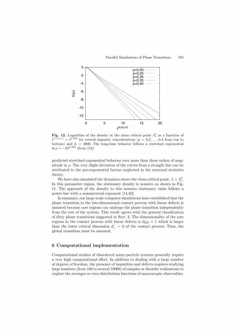
Parallel Simulations of Phase Transitions 195
-12
-10
-8
-6
-4
-2
0
0 5 10 15 20
ln(ρ
)
t(dr/dr+z)
p=0.20p=0.25p=0.30p=0.35p=0.40
Fig. 12. Logarithm of the density at the clean critical point λ0c as a function of
t1/(1+z) = t0.362 for several impurity concentrations (p = 0.2, . . . , 0.4 from top tobottom) and L = 3000. The long-time behavior follows a stretched exponentialln ρ = −Et0.362 (from [14])
predicted stretched exponential behavior over more than three orders of mag-nitude in ρ. The very slight deviation of the curves from a straight line can beattributed to the pre-exponential factors neglected in the extremal statisticstheory.
We have also simulated the dynamics above the clean critical point, λ > λ0c .
In this parameter region, the stationary density is nonzero as shown in Fig.11. The approach of the density to this nonzero stationary value follows apower-law with a nonuniversal exponent [14,62].
In summary, our large-scale computer simulations have established that thephase transition in the two-dimensional contact process with linear defects issmeared because rare regions can undergo the phase transition independentlyfrom the rest of the system. This result agrees with the general classificationof dirty phase transitions suggested in Sect. 2. The dimensionality of the rareregions in the contact process with linear defects is dRR = 1 which is largerthan the lower critical dimension d−c = 0 of the contact process. Thus, theglobal transition must be smeared.
6 Computational implementation
Computational studies of disordered many-particle systems generally requirea very high computational effort. In addition to dealing with a large numberof degrees of freedom, the presence of impurities and defects requires studyinglarge numbers (from 100 to several 10000) of samples or disorder realizations toexplore the averages or even distribution functions of macroscopic observables.
196 Thomas Vojta
Fortunately, this very complication also makes disordered many-particlesystems ideal candidates for massive parallel simulations. In the simplest case,one can distribute (farm out) the Nsamp disorder realizations over the NCPU
available processors at the beginning such that each processor is assignedNsamp/NCPU samples. This can be done, e.g., by using different randomnumber seeds in the function that generates the impurities or defects. Thesimulations then proceed independently for the different samples, minimiz-ing the communication requirements. After each processor has carried outthe simulation for all the samples assigned to it, the data are collected andprocessed to obtain the desired averages or distribution functions. In this way,one achieves linear speedup (total time inversely proportional to the numberof available processors) as long as the number of simulated samples is largerthan the number of processors.
The only major drawback of this scheme lies in the fact that depending onthe algorithm, different samples of a strongly disordered system may requirevastly different simulation times. If the number of samples per processor isfixed from the outset, some idle time is thus unavoidable. To overcome thisproblem we have implemented an algorithm that dynamically assigns the sam-ples to available processors. In the beginning, a master process hands each ofthe simulation processes a specific sample (i.e., a random number seed). Aftera process finishes the simulation, it sends the results to the master processand is handed a new sample. This is repeated until all samples have beensimulated. With this modification of the simple farming process, no cyclesare wasted, and the speedup of our simulations is nearly perfect. In all otheraspects, the simulations use established procedures for parallel computing, inparticular, communication is via MPI.
Monte-Carlo simulations of large many-particle systems with quenched dis-order require huge numbers of (pseudo) random numbers. The quality of therandom number generator (long period, low correlations) is therefore of par-ticular importance. Our main “work horse” generator has been the combinedlinear feedback shift register generator LFSR113 suggested by P. L’Ecuyer [32]which is very fast and has a long period of about 2113. We have also used otherrandom number generators for comparison and testing purposes including thepopular RAN2 from Ref. [45].
7 Summary and conclusions
In this chapter we have discussed the results of large-scale parallel Monte-Carlo simulations of quantum and classical phase transitions with quencheddisorder. We have paid particular attention to the effects of rare strong spa-tial disorder fluctuations, the so-called rare regions. Our results show thatdisorder correlations, either in space or in imaginary time (at quantum phasetransitions) strongly enhance the disorder effects.
Parallel Simulations of Phase Transitions 197
We have focused on what is arguably the simplest type of phase transitionin the presence of impurities and defects, viz., order-disorder transitions withrandom-Tc (random mass) type disorder. In this scenario, both phases areconventional (i.e., disorder is irrelevant at the stable fixed points correspond-ing to the bulk phases). The only disorder effect is a local variation of thetendency towards the ordered phase. For such transitions (with short-rangespatial interactions), a general classification of rare region effects has beensuggested, based on the effective dimensionality dRR of the rare regions [63].Three cases can be distinguished.
(i) If dRR is below the lower critical dimension d−c of the problem, the rareregion effects are exponentially small because the probability of a rare regiondecreases exponentially with its volume but the contribution of each regionto observables increases only as a power law. In this case, the critical point isof conventional power-law type.
(ii) In the second class, with dRR = d−c , the Griffiths effects are of power-law type because the exponentially rarity of the rare regions in Lr is overcomeby an exponential increase of each region’s contribution. In this class, thecritical point is controlled by an infinite-randomness fixed point with activatedscaling.
(iii) Finally, for dRR > d−c , the rare regions can undergo the phase transi-
tion independently from the bulk system. This leads to a destruction of thesharp phase transition by smearing.
All the examples discussed in this chapter are in agreement with this clas-sification. The diluted bilayer quantum Heisenberg antiferromagnet falls intothe first class, because dRR = 1 (disorder correlations in imaginary time di-rection) but d−c = 2 for Heisenberg symmetry. The contact process with pointdefects belongs to class (ii) since dRR = d−c = 0. Finally, the classical Isingmodel with plane defects and the contact process with line defects have asmeared transition, case (iii). In the former system, the plane defects lead todRR = 2 while d−c = 1 for Ising symmetry; in the latter system dRR = 1 butd−c = 0. Thus, all our simulation results provide support for the classificationput forward in Ref. [63].
In conclusion, rare regions, i.e. rare strong spatial disorder fluctuations,can have pronounced effects on phase transitions in systems with quencheddisorder. These effects range from classical Griffiths phenomena to the muchstronger quantum Griffiths singularities, and to a complete destruction of thesharp phase transition by smearing. The simulation results summarized herehave helped clarifying these rare region effects for order-disorder transitionsbetween conventional phases. In the future, it will be interesting to see whetheradditional new rare region effects [63] can be found for transitions where thephases themselves are unconventional, such as spin glass or random singletphases.
198 Thomas Vojta
Acknowledgements
The research presented here would have been impossible without the contri-butions and suggestions of many friends and colleagues including D. Belitz,T.R. Kirkpatrick, J. Schmalian, M. Schreiber, R. Sknepnek, and M. Vojta.
This work was supported in part by SFB 393 of the German ResearchFoundation, by the National Science Foundation under grant no. DMR-0339147 and by the University of Missouri Research Board. Thomas Vojtais a Cottrell Scholar of Research Corporation.
The early simulations for this work have been performed on the CLICcluster at Chemnitz University of Technology, the later calculations have beencarried out on the PEGASUS cluster in the Physics Department at the Uni-versity of Missouri-Rolla. The author is also grateful for the hospitality ofthe Aspen Center for Physics and the Kavli Institute for Theoretical Physics,Santa Barbara (supported by the NSF via grant no. PHY99-07949), whereparts of the work have been performed.
References
1. Aharony, A., Harris, A.B.: Absence of Self-averaging and universal fluctuationsin random systems near critical points. Phys. Rev. Lett., 77:3700, 1996.
2. Boyanovsky D., Cardy, J.L.: Critical behavior of m-component magnets withcorrelated impurities. Phys. Rev. B 26:154, 1982.
3. Ballesteros, H.G., Fernandez, L.A., Martın-Mayor, V., Munoz Sudupe, A.: Crit-ical exponents of the three-dimensional diluted Ising model. Phys. Rev. B,58:2740, 1998.
4. Bray, A.J., Huifang, D.: Griffiths singularities in random magnets: Results fora soluble model. Phys. Rev. B, 40:6980, 1989.
5. Bhatt, R.N., Lee, P.A.: Scaling Studies of Highly Disordered Spin-1/2 Antifer-romagnetic Systems. Phys. Rev. Lett., 48:344, 1982.
6. Bray A.J., Rodgers, G.J.: Dynamics of random ising ferromagnets in the Griffithsphase. Phys. Rev. B, 38:9252, 1988.
7. Bray, A.J.: Nature of the Griffiths phase. Phys. Rev. Lett., 59:586, 1987.8. Bray, A.J.: Dynamics of dilute magnets above Tc. Phys. Rev. Lett., 60:720, 1988.9. Chopard B., Droz, M.: Cellular Automaton Modeling of Physical Systems. Cam-
bridge University Press, Cambridge, 1998.10. Chakravarty, S., Halperin, B.I., Nelson, D.R.: Two-dimensional quantum Heisen-
berg antiferromagnet at low temperatures. Phys. Rev. B, 39:2344, 1989.11. Dickman, R.: Reweighting in nonequilibrium simulations. Phys. Rev. E,
60:R2441, 1999.12. Dobrosavljevic V., Miranda, E.: Absence of Conventional Quantum Phase Tran-
sitions in Itinerant Systems with Disorder. Phys. Rev. Lett., 94:187203, 2005.13. Dhar, D., Randeria, M., Sethna, J.: Griffiths singularities in the dynamics of
disordered Ising models. Europhys. Lett., 5:485, 1988.14. Dickison, M, Vojta, T.: Monte Carlo simulations of the smeared phase transition
in a contact process with extended defects. J. Phys. A, 38:1199, 2005.
Parallel Simulations of Phase Transitions 199
15. Fisher, D.S.: Random transverse-field Ising spin chains. Phys. Rev., 69:534, 1992.16. Fisher, D.S.: Random antiferromagnetic quantum spin chains. Phys. Rev. B,
50:3799, 1994.17. Fisher, D.S.: Critical behavior of random transverse-field Ising spin chains. Phys.
Rev. B, 51:6411, 1995.18. Ferrenberg A.M., Landau, D.P.: Critical behavior of the three-dimensional Ising
model: A high-resolution Monte Carlo study. Phys. Rev. B, 44:5081, 1991.19. Guo, M., Bhatt R., Huse, D.: Quantum Griffiths singularities in the transverse-
field Ising spin glass. Phys. Rev. B, 54:3336, 1996.20. Grassberger, P.: On phase transitions in Schlogl’s second model. Z. Phys. B,
47:365, 1982.21. Griffiths, R.B.: Nonanalytic behavior above the critical point in a random Ising
ferromagnet. Phys. Rev. Lett., 23:17, 1969.22. Grinstein, G.: Phases and phase transitions of quenched disordered systems. In:
Cohen, E.G.D. (ed) Fundamental Problems in Statistical Mechanics VI. Elsevier,New York (1985) p.147
23. Grassberger, P., de la Torre, A.: Reggeon field theory (Schlogl’s first model)on a lattice: Monte Carlo calculations of critical behaviour. Ann. Phys. (NY),122:373 , 1979.
24. Harris, A.B.: Effect of random defects on the critical behaviour of Ising models.J. Phys. C, 7:1671, 1974.
25. Harris, T.E.: Contact interactions on a lattice. Ann. Prob., 2:969, 1974.26. Hida, K.: Low temperature properties of the double layer quantum Heisenberg
antiferromagnet-modified spin wave method. J. Phys. Soc. Jpn., 59:2230, 1990.27. Hinrichsen, H.: Non-equilibrium critical phenomena and phase transitions into
absorbing states. Adv. Phys., 49:815, 2000.28. Hooyberghs, J., Igloi, F., Vanderzande, C.: Strong Disorder Fixed Point in
Absorbing-State Phase Transitions. Phys. Rev. Lett., 90:100601, 2003.29. Holm C., Janke, W.: Critical exponents of the classical three-dimensional Heisen-
berg model: A single-cluster Monte Carlo study. Phys. Rev. B, 48:936, 1993.30. Janssen, H.K.: On the nonequilibrium phase transition in reaction-diffusion sys-
tems with an absorbing stationary state. Z. Phys. B, 42:151, 1981.31. Janssen, H.K.: Renormalized field theory of the Gribov process with quenched
disorder. Phys. Rev. E, 55:6253, 1997.32. L’Ecuyer, P.: Tables of maximally-equidistributed combined LFSR generators.
Mathematics of Computation,, 68:225, 261, 1999.33. Lubensky, T.C: Critical properties of random-spin models from the epsilon ex-
pansion. Phys. Rev. B, 11:3573, 1975.34. McCoy, B.M.: Incompleteness of the Critical Exponent Description for Fer-
romagnetic Systems Containing Random Impurities. Phys. Rev. Lett., 23:383,1969.
35. Marro, J., Dickman, R.: Nonequilibrium Phase Transitions in Lattice Models.Cambridge University Press, Cambridge (1996)
36. Moreira, A.G., Dickman, R.: Critical dynamics of the contact process withquenched disorder. Phys. Rev. E, 54:R3090 , 1996.
37. Ma, S.K., Dasgupta, C., Hu, C.-K.: Random antiferromagnetic chain. Phys. Rev.Lett., 43:1434 , 1979.
38. Millis, A.J., Monien, H.: Spin Gaps and Spin Dynamics in La2−xSrxCuO4 andYBa2Cu3O7−δ. Phys. Rev. Lett., 70:2810, 1993.
200 Thomas Vojta
39. Motrunich, O., Mau, S.-C., Huse, D.A., Fisher, D.S.: Infinite-randomness quan-tum Ising critical fixed points. Phys. Rev. B, 61:1160, 2000.
40. Millis, A.J., Morr, D.K., Schmalian, J.: Local Defect in Metallic Quantum Crit-ical Systems. Phys. Rev. Lett., 87:167202, 2001.
41. Millis, A.J., Morr, D.K., Schmalian, J.: Quantum Griffiths effects in metallicsystems. Phys. Rev. B, 66:174433, 2002.
42. McCoy B.M., Wu, T.T.: Theory of a Two-Dimensional Ising Model with Ran-dom Impurities. I. Thermodynamics. Phys. Rev., 176:631, 1968.
43. Noest, A.J.: New universality for spatially disordered cellular automata anddirected percolation. Phys. Rev. Lett., 57:90, 1986.
44. Odor G.: Universality classes in nonequilibrium lattice systems. Rev. Mod. Phys.,76:663, 2004.
45. Press, W.H., Teukolsky, S.A., Vetterling, W.T., Flannary, B.P.: NumericalRecipes in Fortran. Cambridge University Press, Cambridge (1992)
46. Pich, C., Young, A.P., Rieger, H., Kawashima, N.: Critical behavior andGriffiths-McCoy singularities in the two-dimensional random quantum Ising fer-romagnet. Phys. Rev. Lett., 81:5916, 1998.
47. Randeria, M., Sethna, J., Palmer, R.G.: Low-Frequency Relaxation in Ising Spin-Glasses. Phys. Rev. Lett., 54:1321, 1985.
48. Rieger, H., Young, A.P.: Griffiths Singularities in the Disordered Phase of aQuantum Ising Spin Glass. Phys. Rev. B, 54:3328, 1996.
49. Sachdev, S.: Quantum Phase Transitions. Cambridge University Press, Cam-bridge (1999)
50. Sandvik, A.W.: Multicritical Point in a Diluted Bilayer Heisenberg QuantumAntiferromagnet. Phys. Rev. Lett., 89:177201, 2002.
51. Sandvik, A.W., Scalapino, D.J.: Order-disorder transition in a two-layer quan-tum antiferromagnet. Phys. Rev. Lett., 72:2777, 1994.
52. S. Sachdev and M. Vojta, Non-magnetic impurities as probes of insulating anddoped Mott insulators in two dimensions. In: Fokas, A. et al (Eds.): Proceedingsof the XIII International Congress on Mathematical Physics. International Press,Boston (2001).
53. Sknepnek, R., Vojta, T.: Smeared phase transition in a three-dimensional Isingmodel with planar defects: Monte-Carlo simulations. Phys. Rev. B, 69:174410,2004.
54. Sknepnek, R., Vojta, T., Vojta, M.: Exotic vs. conventional scaling and univer-sality in a disordered bilayer quantum Heisenberg antiferromagnet. Phys. Rev.Lett., 93:097201, 2004.
55. Schmittmann B., Zia, R.K.P.: Statistical mechanics of driven diffusive systems.In: Domb, C., Lebowitz, J.L.: Phase transitions and critical phenomena, Vol.17. Academic Press, New York (1995)
56. Thill M., Huse D.: Equilibrium behaviour of quantum Ising spin glass. PhysicaA , 214:321, 1995.
57. Tauber, U.C., Howard, M., Vollmayr-Lee, B.P.: Applications of field-theoreticrenormalization group methods to reaction-diffusion problems. J. Phys. A,38:R79, 2005.
58. Vojta, T., Dickison, M.: Critical behavior and Griffiths effects in the disoderedcontact process. Phys. Rev. E, 72:036126, 2005.
59. Vajk, O.P., Greven, M.: Quantum Versus Geometric Disorder in a Two-Dimensional Heisenberg Antiferromagnet. Phys. Rev. Lett., 89:177202, 2002.
Parallel Simulations of Phase Transitions 201
60. Vojta. T.: Disorder induced rounding of certain quantum phase transitions.Phys. Rev. Lett., 90:107202, 2003.
61. Vojta, T.: Smearing of the phase transition in Ising systems with planar defects.J. Phys. A, 36:10921, 2003.
62. Vojta, T.: Broadening of a nonequilibrium phase transition by extended struc-tural defects. Phys. Rev. E, 70:026108, 1994.
63. Vojta, T., Schmalian, S.: Quantum Griffiths effects in itinerant Heisenberg mag-nets. Phys. Rev. B, 72:045438, 2005.
64. Voigt, C.A., Ziff, R.M.: Epidemic analysis of the second-order transition in theZiff-Gulari-Barshad surface-reaction model. Phys. Rev. E, 56:R6241, 1997.
65. Wiseman S., Domany E.: Finite-size scaling and Lack of self-averaging in criticaldisordered systems. Phys. Rev. Lett., 81:22, 1998.
66. Wolff, U.: Collective Monte Carlo updating for spin systems. Phys. Rev. Lett.,62:361, 1989.
67. Young, A.P., Rieger, H.: Numerical study of the random transverse-field Isingspin chain. Phys. Rev. B, 53:8486, 1996.

Localization of Electronic States in AmorphousMaterials: Recursive Green’s Function Methodand the Metal-Insulator Transition at E = 0
Alexander Croy1, Rudolf A. Romer2, and Michael Schreiber1
1 Technische Universitat Chemnitz, Institut fur Physik09107 Chemnitz, [email protected], [email protected]
2 Centre for Scientific Computing and Department of PhysicsUniversity of Warwick, Coventry, CV4 7AL, United [email protected]
1 Introduction
Traditionally, condensed matter physics has focused on the investigation ofperfect crystals. However, real materials usually contain impurities, disloca-tions or other defects, which distort the crystal. If the deviations from theperfect crystalline structure are large enough, one speaks of disordered sys-tems. The Anderson model [1] is widely used to investigate the phenomenon oflocalisation of electronic states in disordered materials and electronic trans-port properties in mesoscopic devices in general. Especially the occurrenceof a quantum phase transition driven by disorder from an insulating phase,where all states are localised, to a metallic phase with extended states, hasled to extensive analytical and numerical investigations of the critical prop-erties of this metal-insulator transition (MIT) [2–4]. The investigation of thebehaviour close to the MIT is supported by the one-parameter scaling hypoth-esis [5,6]. This scaling theory originally formulated for the conductance playsa crucial role in understanding the MIT [7]. It is based on an ansatz inter-polating between metallic and insulating regimes [8]. So far, scaling has beendemonstrated to an astonishing degree of accuracy by numerical studies of theAnderson model [9–13]. However, most studies focused on scaling of the local-isation length and the conductivity at the disorder-driven MIT in the vicinityof the band centre [9,14,15]. Assuming a power-law form for the d.c. conduc-tivity, as it is expected from the one-parameter scaling theory, Villagonzalo etal. [6] have used the Chester-Thellung-Kubo-Greenwood formalism to calcu-late the temperature dependence of the thermoelectric properties numericallyand showed that all thermoelectric quantities follow single-parameter scalinglaws [16,17].
204 Alexander Croy et al.
In this chapter we will investigate whether the scaling assumptions madein previous studies for the transition at energies outside the band centre can bereconfirmed in numerical calculations, and in particular whether the conduc-tivity σ follows a power law close to the critical energy Ec. For this purpose wewill use the recursive Green’s function method [18, 19] to calculate the four-terminal conductance of a disordered system for fixed disorder strength attemperature T = 0. Applying the finite-size scaling analysis we will computethe critical exponent and determine the mobility edge, i.e. the MIT outsidethe band centre. A complementary investigation into the statistics of the en-ergy spectrum and the states close to the MIT can be found in Chap. [20].An analysis of the mathematical properties of the so-called binary-alloy orBernoulli-Anderson model is done in Chap. [21].
2 The Anderson model of localisationand its metal-insulator transition
The Anderson model [1, 2] is widely used to investigate the phenomenon oflocalisation of electronic states in disordered materials. It is based upon atight-binding Hamiltonian in site representation
H =∑
i
ǫi|i〉〈i|+∑
i=j
tij |i〉〈j| , (1)
where |i〉 is a localized state at site i and tij are the hopping parameters, whichare usually restricted to nearest neighbours. The on-site potentials ǫi are ran-dom numbers, chosen according to some distribution P (ǫ) [22, 23]. In whatfollows we take P (ǫ) to be a box distribution over the interval [−W/2,W/2],thus W determines the strength of the disorder in the system. Other distrib-utions have also been considered [2, 3, 24].
For strong enough disorder, W > Wc(E = 0), all states are exponentiallylocalized and the respective wave functions Ψ(r) are proportional to e−|r−r0|/ξ
for large distances |r− r0|. Thus, Ψ is confined to a region of some finite size,which may be described by the so-called localisation length ξ. In this languageextended states are characterised by ξ −→ ∞. Comparing ξ with the size Lof the system one can distinguish between strong and weak localisation, forξ ≪ L and L < ξ, respectively3. Here we also assume that the phase-relaxationlength ℓΦ ≫ L. Otherwise, the effective system size is determined by ℓΦ.
It turns out that the value of the critical disorder strength Wc depends onthe distribution function P (ε) and the dimension d of the system. In absence
3We note that the phrase weak localization in the context of the scaling theoryis often used with a specific meaning, namely the onset of localization in large 2-dimensional samples, where the conductance decreases logarithmically with scale[2, 7].
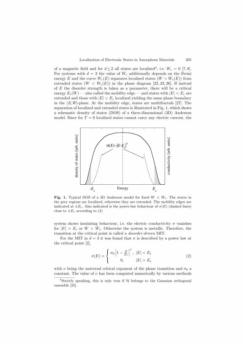
Localization of Electronic States in Amorphous Materials 205
of a magnetic field and for d≤ 2 all states are localized4, i.e. Wc = 0 [7, 8].For systems with d = 3 the value of Wc additionally depends on the Fermienergy E and the curve Wc(E) separates localized states (W > Wc(E)) fromextended states (W < Wc(E)) in the phase diagram [22, 23, 26]. If insteadof E the disorder strength is taken as a parameter, there will be a criticalenergy Ec(W ) — also called the mobility edge — and states with |E| < Ec areextended and those with |E| > Ec localized yielding the same phase boundaryin the (E,W)-plane. At the mobility edge, states are multifractals [27]. Theseparation of localized and extended states is illustrated in Fig. 1, which showsa schematic density of states (DOS) of a three-dimensional (3D) Andersonmodel. Since for T = 0 localized states cannot carry any electric current, the
Energy
dens
ity
of s
tate
s [a
rb. u
nits
]
cond
ucti
vity
[ar
b. u
nits
]
-Ec
Ec
σ(E)∼|E-Ec|ν
Fig. 1. Typical DOS of a 3D Anderson model for fixed W < Wc. The states inthe grey regions are localized, otherwise they are extended. The mobility edges areindicated at ±Ec. Also indicated is the power-law behaviour of σ(E) (dashed lines)close to ±Ec according to (2)
system shows insulating behaviour, i.e. the electric conductivity σ vanishesfor |E| > Ec or W > Wc. Otherwise the system is metallic. Therefore, thetransition at the critical point is called a disorder-driven MIT.
For the MIT in d = 3 it was found that σ is described by a power law atthe critical point [2],
σ(E) =
σ0
∣∣∣1− EEc
∣∣∣ν
, |E| < Ec
0, |E| > Ec
(2)
with ν being the universal critical exponent of the phase transition and σ0 aconstant. The value of ν has been computed numerically by various methods
4Strictly speaking, this is only true if H belongs to the Gaussian orthogonalensemble [25].
206 Alexander Croy et al.
[2,9–11] and was also derived from experiments [28,29]. The results range from1 to 1.6, depending on the distribution P (ǫ) and the computational method [3]used.
Moreover, Wegner [30] was able to show that for non-interacting electronsthe d.c. conductivity σ obeys a general scaling form close to the MIT,
σ(ε, ω) = b2−d σ(b1/νε, bzω) . (3)
Here ε denotes the dimensionless distance from the critical point, ω is anexternal parameter such as the frequency or the temperature, b is a scalingparameter and z is the dynamical exponent. For non-interacting electronsz = d [31]. Assuming a finite conductivity for ω = 0, one obtains from (3)
σ(ε, 0) ∝ εν(d−2), (4)
where ε = |1− E/Ec|. With d = 3 this gives (2).
3 Computational method
An approach to calculate the d.c. conductivity from the Anderson tight-binding Hamiltonian (1) is the recursive Green’s function method [18,19,23].It yields a recursion scheme for the d.c. conductivity tensor starting fromthe Kubo-Greenwood formula [32]. Moreover, this method allows to com-pute the density of states and the localization length as well as the fullset of thermoelectric kinetic coefficients [33]. Parallel implementations of themethod are advantageous [34,35]. The method is therefore a companion to themore widely used transfer-matrix method [36, 37] or iterative diagonalisationschemes [38,39].
3.1 Recursive Green’s function method
Let H =∑
ij Hij |i〉〈j| denote our hermitian tight-binding Hamiltonian. The
single particle Green’s function G±(z) is defined as [40] (z±−H)G± = 1 wherez = E ± iγ is the complex energy and the sign of the small imaginary part γdistinguishes between advanced and retarded Green’s functions, G−(E − i0)and G+(E + i0), respectively [40]. Equivalently, G± can be represented in thebasis of the functions |i〉,
(z±δij −Hij)G±ij = δij , (5)
where G±ij is the matrix element 〈i|G±|j〉. We note that for a hermitian Hamil-
tonian G−ij = (G+
ji)∗.
If H contains only nearest-neighbour hopping matrix elements, (5) can besimplified using a block matrix notation. This is equivalent to considering thesystem as being built up of slices or strips for 3D or 2D, respectively, along
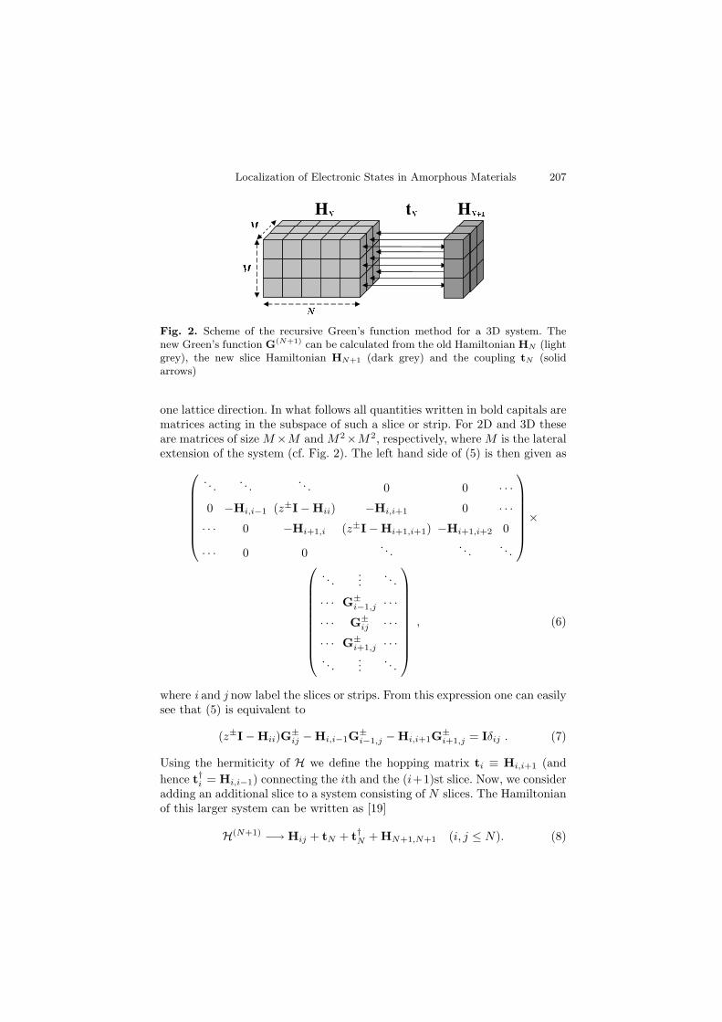
Localization of Electronic States in Amorphous Materials 207
Fig. 2. Scheme of the recursive Green’s function method for a 3D system. Thenew Green’s function G(N+1) can be calculated from the old Hamiltonian HN (lightgrey), the new slice Hamiltonian HN+1 (dark grey) and the coupling tN (solidarrows)
one lattice direction. In what follows all quantities written in bold capitals arematrices acting in the subspace of such a slice or strip. For 2D and 3D theseare matrices of sizeM×M andM2×M2, respectively, whereM is the lateralextension of the system (cf. Fig. 2). The left hand side of (5) is then given as
. . .. . .
. . . 0 0 · · ·0 −Hi,i−1 (z±I−Hii) −Hi,i+1 0 · · ·· · · 0 −Hi+1,i (z±I−Hi+1,i+1) −Hi+1,i+2 0
· · · 0 0. . .
. . .. . .
×
. . ....
. . .
· · · G±i−1,j · · ·
· · · G±ij · · ·
· · · G±i+1,j · · ·
. . ....
. . .
, (6)
where i and j now label the slices or strips. From this expression one can easilysee that (5) is equivalent to
(z±I−Hii)G±ij −Hi,i−1G
±i−1,j −Hi,i+1G
±i+1,j = Iδij . (7)
Using the hermiticity of H we define the hopping matrix ti ≡ Hi,i+1 (and
hence t†i = Hi,i−1) connecting the ith and the (i+1)st slice. Now, we consideradding an additional slice to a system consisting of N slices. The Hamiltonianof this larger system can be written as [19]
H(N+1) −→ Hij + tN + t†N + HN+1,N+1 (i, j ≤ N). (8)
208 Alexander Croy et al.
The first and the last terms describe the uncoupled N -slice and the additional1-slice system. Using tN as an “interaction” the Green’s function G(N+1) ofthe coupled system can be calculated via Dyson’s equation [19,40],
G(N+1)ij = G
(N)ij + G
(N)iN tNG
(N+1)Nj (i, j ≤ N). (9)
In particular, we have
G(N+1)N+1,N+1 =
[z±I−HN+1,N+1 − t†NG
(N)NNtN
]−1
(10a)
G(N+1)ij = G
(N)ij + G
(N)iN tNG
(N+1)N+1,N+1t
†NG
(N)Nj (i, j ≤ N) (10b)
G(N+1)i,N+1 = G
(N)iN tNG
(N+1)N+1,N+1 (i ≤ N) (10c)
G(N+1)N+1,j = G
(N+1)N+1,N+1t
†NG
(N)Nj (j ≤ N) . (10d)
With (10) the Green’s function can be obtained iteratively. Additionally, thereare two kinds of boundary conditions which must be considered: across eachslice and at the beginning and the end of the stack. The first kind does notpresent any difficulty and usually hard wall or periodic boundary conditionsare employed. The second kind of boundary is connected to some subtletieswith attached leads which will be addressed in Sect. 6.
3.2 Density of states and d.c. conductivity
The DOS is given in terms of Green’s function by [40]
ρ(E) = − 1
πΩImTrG+ = − 1
πNM 2Im
N∑
i=1
TrG+ii (11)
and the d.c. conductivity σ is
σ =2e2
πΩm2Tr
[p ImG+ p ImG+
]. (12)
Here, Ω denotes the volume of the system and m the electron mass. Usingfor the momentum the relation p = im
[H, x] one can rewrite (12) in position
representation
σ =e24
hNM2Tr
γ2
N∑
i,j
G+ij xj G−
ji xi − iγ
2
N∑
i
(G+ii −G−
ii ) x 2i
, (13)
where xi is the position of the ith slice.Starting from these relations and using the iteration scheme (10) one can
derive recursion formulæ to calculate the properties for the (N + 1)-slice sys-tem. The results are expressed in terms of the following auxiliary matrices
Localization of Electronic States in Amorphous Materials 209
RN = G+N,N , (14a)
BN = γt†N
N∑
ij
G+(N)Nj xj(2γG
−(N)ji − iIδij)xiG
+(N)iN
tN , (14b)
C+N = γt†N
[N∑
i=1
G+(N)Ni xiG
−(N)iN
]tN = (C+
N )† , (14c)
C−N = γt†N
[N∑
i=1
G−(N)Ni xiG
+(N)iN
]tN = (C−
N )† , (14d)
FN = t†N
[N∑
i=1
G+(N)Ni G
+(N)iN
]tN . (14e)
The derivation can be simplified assuming the new slice to be at xN+1 = 0.This leads, however, to corrections for the matrices BN and C±
N because theorigin of xi has to be shifted to the position of the current slice in each iterationstep. The corrections are
B′N = BN + iC+
N + iC−N +
1
2t†N (RN −R†
N )tN , (15a)
C′±N = C±
N − i1
2t†N (RN −R†
N )tN . (15b)
Here we have used the identity
γ
N∑
i=1
G+NiG
−iN = i
1
2(G+
NN −G−NN ) = i
1
2(RN −R†
N ) = −ImRN . (16)
The derivation of the recursion relations is given in Refs. [18, 19, 23, 41], ityields the following expressions
s(N+1)ρ = s(N)
ρ + Tr RN+1(FN + I) , (17a)
s(N+1)σ = s(N)
σ + Tr Re (BNRN+1) + C+NR†
N+1C−NRN+1 , (17b)
RN+1 =[z±I−HN+1,N+1 − t†NRNtN
]−1
, (17c)
BN+1 = t†N+1RN+1
[BN + 2C+
NR†N+1C
−N
]RN+1tN+1 , (17d)
C+N+1 = t†N+1RN+1C
+NR†
N+1tN+1 , (17e)
C−N+1 = t†N+1R
†N+1C
−NRN+1tN+1 , (17f)
FN+1 = t†N+1RN+1(FN + I)RN+1tN+1 . (17g)
The DOS and the d.c. conductivity are then given as

210 Alexander Croy et al.
ρ(N+1)(E) = − 1
π(N + 1)M2s(N+1)
ρ , (18)
σ(N+1)(E) =e2
h
4
(N + 1)M2s(N+1)
σ . (19)
For a comparison with the scaling arguments, we convert the conductivityinto the two-terminal conductance as
g2 = σM2
L(20)
with L = N + 1. In distinction to the usual use of the recursive scheme whichconstructs a single sample with L ≫ M , we shall have to use many differentcubic samples with L =M .
We note that it is also possible to calculate the localisation length ξ(E) bythe Green’s function method. The value of ξ(E) is connected to the matrixG+
1N+1,1
ξ(E)= − lim
γ→0lim
N→∞
1
2Nln∣∣TrG+
1N (E )∣∣2 . (21)
The recursion relation for ξ(N+1)(E) is
1
ξ(N+1)(E)= − 1
N + 1s(N+1)ξ , (22a)
s(N+1)ξ = s
(N)ξ + ln
∣∣∣TrG+(N+1)N+1,N+1
∣∣∣ . (22b)
4 Finite-size scaling
For finite systems there can be no singularities induced by a phase transitionand the divergences at the MIT are always rounded off [42]. Fortunately,the MIT can still be studied using a technique known as finite-size scaling [2].Here we briefly review the main results taking the dimensionless four-terminalconductance g4 of a large cubic sample of size L× L× L as an example. Wenote that similar scaling ideas can also be applied to the reduced localisationlength ξ/L. In order to obtain g4 of the disordered region only, we have tosubtract the contact resistance due to the leads. This gives
1
g4=
1
g2− 1
N . (23)
Here N = N (E) is the number of propagating channels at the Fermi energyE which is determined by the quantization of wave numbers in transversedirection in the leads [43,44].
Near the MIT one expects a one-parameter scaling law for the dimension-less conductance [7, 30,42]
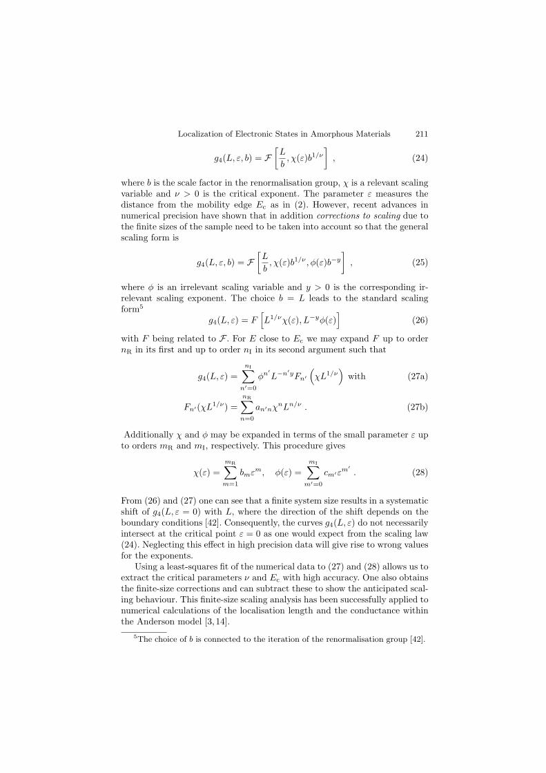
Localization of Electronic States in Amorphous Materials 211
g4(L, ε, b) = F[L
b, χ(ε)b1/ν
], (24)
where b is the scale factor in the renormalisation group, χ is a relevant scalingvariable and ν > 0 is the critical exponent. The parameter ε measures thedistance from the mobility edge Ec as in (2). However, recent advances innumerical precision have shown that in addition corrections to scaling due tothe finite sizes of the sample need to be taken into account so that the generalscaling form is
g4(L, ε, b) = F[L
b, χ(ε)b1/ν , φ(ε)b−y
], (25)
where φ is an irrelevant scaling variable and y > 0 is the corresponding ir-relevant scaling exponent. The choice b = L leads to the standard scalingform5
g4(L, ε) = F[L1/νχ(ε), L−yφ(ε)
](26)
with F being related to F . For E close to Ec we may expand F up to ordernR in its first and up to order nI in its second argument such that
g4(L, ε) =
nI∑
n′=0
φn′
L−n′yFn′
(χL1/ν
)with (27a)
Fn′(χL1/ν) =
nR∑
n=0
an′nχnLn/ν . (27b)
Additionally χ and φ may be expanded in terms of the small parameter ε upto orders mR and mI, respectively. This procedure gives
χ(ε) =
mR∑
m=1
bmεm, φ(ε) =
mI∑
m′=0
cm′εm′
. (28)
From (26) and (27) one can see that a finite system size results in a systematicshift of g4(L, ε = 0) with L, where the direction of the shift depends on theboundary conditions [42]. Consequently, the curves g4(L, ε) do not necessarilyintersect at the critical point ε = 0 as one would expect from the scaling law(24). Neglecting this effect in high precision data will give rise to wrong valuesfor the exponents.
Using a least-squares fit of the numerical data to (27) and (28) allows us toextract the critical parameters ν and Ec with high accuracy. One also obtainsthe finite-size corrections and can subtract these to show the anticipated scal-ing behaviour. This finite-size scaling analysis has been successfully applied tonumerical calculations of the localisation length and the conductance withinthe Anderson model [3, 14].
5The choice of b is connected to the iteration of the renormalisation group [42].
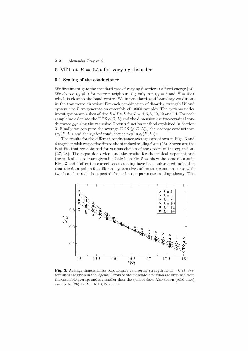
212 Alexander Croy et al.
5 MIT at E = 0.5 t for varying disorder
5.1 Scaling of the conductance
We first investigate the standard case of varying disorder at a fixed energy [14].We choose tij = 0 for nearest neigbours i, j only, set tij = t and E = 0.5 twhich is close to the band centre. We impose hard wall boundary conditionsin the transverse direction. For each combination of disorder strength W andsystem size L we generate an ensemble of 10000 samples. The systems underinvestigation are cubes of size L×L×L for L = 4, 6, 8, 10, 12 and 14. For eachsample we calculate the DOS ρ(E,L) and the dimensionless two-terminal con-ductance g2 using the recursive Green’s function method explained in Section3. Finally we compute the average DOS 〈ρ(E,L)〉, the average conductance〈g4(E,L)〉 and the typical conductance exp〈ln g4(E,L)〉.
The results for the different conductance averages are shown in Figs. 3 and4 together with respective fits to the standard scaling form (26). Shown are thebest fits that we obtained for various choices of the orders of the expansions(27, 28). The expansion orders and the results for the critical exponent andthe critical disorder are given in Table 1. In Fig. 5 we show the same data as inFigs. 3 and 4 after the corrections to scaling have been subtracted indicatingthat the data points for different system sizes fall onto a common curve withtwo branches as it is expected from the one-parameter scaling theory. The
15 15.5 16 16.5 17 17.5 18W/t
0.4
0.6
0.8
1
⟨g 4⟩
L = 4L = 6L = 8L = 10L = 12L = 14
Fig. 3. Average dimensionless conductance vs disorder strength for E = 0.5 t. Sys-tem sizes are given in the legend. Errors of one standard deviation are obtained fromthe ensemble average and are smaller than the symbol sizes. Also shown (solid lines)are fits to (26) for L = 8, 10, 12 and 14
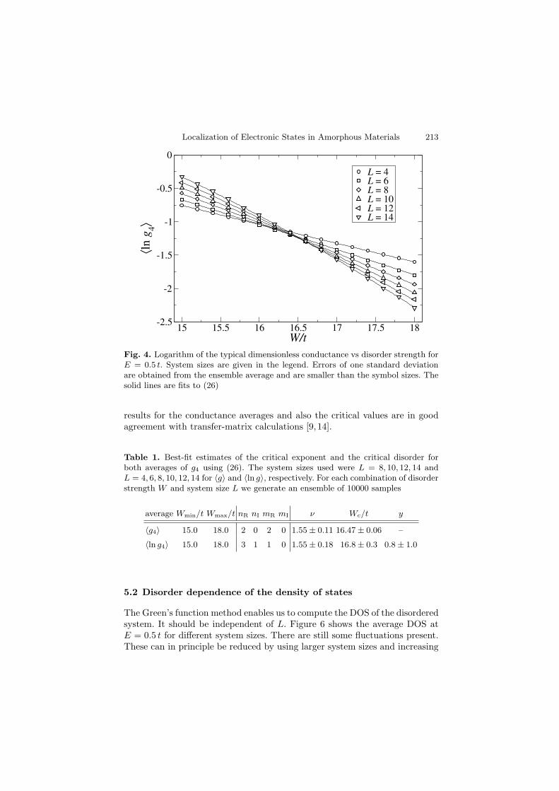
Localization of Electronic States in Amorphous Materials 213
15 15.5 16 16.5 17 17.5 18W/t
-2.5
-2
-1.5
-1
-0.5
0⟨l
n g 4⟩
L = 4L = 6L = 8L = 10L = 12L = 14
Fig. 4. Logarithm of the typical dimensionless conductance vs disorder strength forE = 0.5 t. System sizes are given in the legend. Errors of one standard deviationare obtained from the ensemble average and are smaller than the symbol sizes. Thesolid lines are fits to (26)
results for the conductance averages and also the critical values are in goodagreement with transfer-matrix calculations [9, 14].
Table 1. Best-fit estimates of the critical exponent and the critical disorder forboth averages of g4 using (26). The system sizes used were L = 8, 10, 12, 14 andL = 4, 6, 8, 10, 12, 14 for 〈g〉 and 〈ln g〉, respectively. For each combination of disorderstrength W and system size L we generate an ensemble of 10000 samples
average Wmin/t Wmax/t nR nI mR mI ν Wc/t y
〈g4〉 15.0 18.0 2 0 2 0 1.55 ± 0.11 16.47 ± 0.06 –
〈ln g4〉 15.0 18.0 3 1 1 0 1.55 ± 0.18 16.8 ± 0.3 0.8 ± 1.0
5.2 Disorder dependence of the density of states
The Green’s function method enables us to compute the DOS of the disorderedsystem. It should be independent of L. Figure 6 shows the average DOS atE = 0.5 t for different system sizes. There are still some fluctuations present.These can in principle be reduced by using larger system sizes and increasing
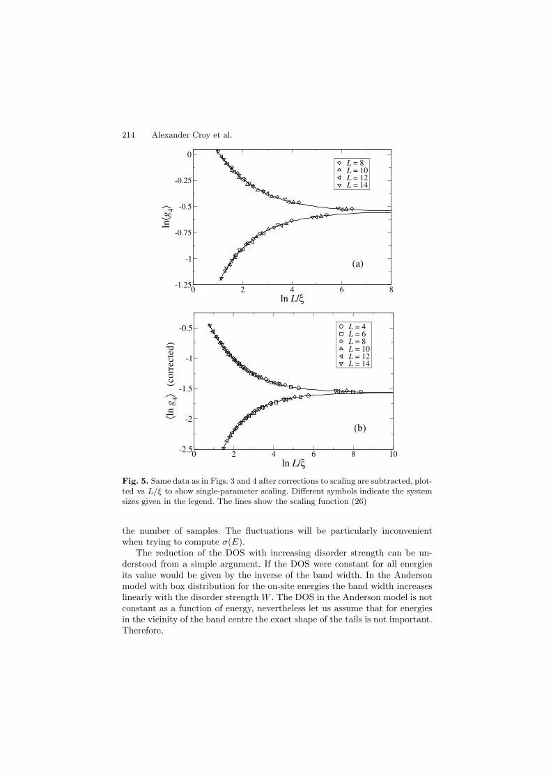
214 Alexander Croy et al.
0 2 4 6 8ln L/ξ
-1.25
-1
-0.75
-0.5
-0.25
0
ln⟨g
4⟩L = 8L = 10L = 12L = 14
(a)
0 2 4 6 8 10ln L/ξ
-2.5
-2
-1.5
-1
-0.5
⟨ln
g 4⟩
(cor
rect
ed)
L = 4L = 6L = 8L = 10L = 12L = 14
(b)
Fig. 5. Same data as in Figs. 3 and 4 after corrections to scaling are subtracted, plot-ted vs L/ξ to show single-parameter scaling. Different symbols indicate the systemsizes given in the legend. The lines show the scaling function (26)
the number of samples. The fluctuations will be particularly inconvenientwhen trying to compute σ(E).
The reduction of the DOS with increasing disorder strength can be un-derstood from a simple argument. If the DOS were constant for all energiesits value would be given by the inverse of the band width. In the Andersonmodel with box distribution for the on-site energies the band width increaseslinearly with the disorder strengthW . The DOS in the Anderson model is notconstant as a function of energy, nevertheless let us assume that for energiesin the vicinity of the band centre the exact shape of the tails is not important.Therefore,
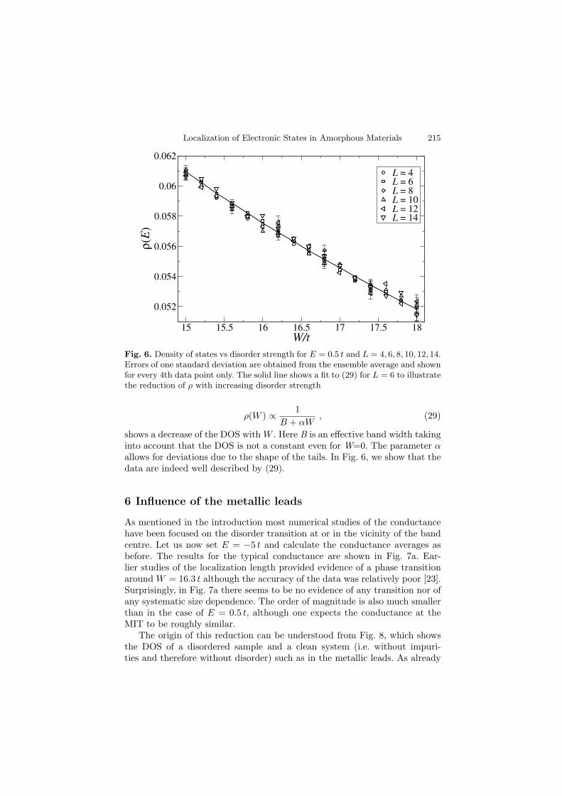
Localization of Electronic States in Amorphous Materials 215
15 15.5 16 16.5 17 17.5 18W/t
0.052
0.054
0.056
0.058
0.06
0.062ρ
(E)
L = 4L = 6L = 8L = 10L = 12L = 14
Fig. 6. Density of states vs disorder strength for E = 0.5 t and L = 4, 6, 8, 10, 12, 14.Errors of one standard deviation are obtained from the ensemble average and shownfor every 4th data point only. The solid line shows a fit to (29) for L = 6 to illustratethe reduction of ρ with increasing disorder strength
ρ(W ) ∝ 1
B + αW, (29)
shows a decrease of the DOS withW . Here B is an effective band width takinginto account that the DOS is not a constant even for W=0. The parameter αallows for deviations due to the shape of the tails. In Fig. 6, we show that thedata are indeed well described by (29).
6 Influence of the metallic leads
As mentioned in the introduction most numerical studies of the conductancehave been focused on the disorder transition at or in the vicinity of the bandcentre. Let us now set E = −5 t and calculate the conductance averages asbefore. The results for the typical conductance are shown in Fig. 7a. Ear-lier studies of the localization length provided evidence of a phase transitionaround W = 16.3 t although the accuracy of the data was relatively poor [23].Surprisingly, in Fig. 7a there seems to be no evidence of any transition nor ofany systematic size dependence. The order of magnitude is also much smallerthan in the case of E = 0.5 t, although one expects the conductance at theMIT to be roughly similar.
The origin of this reduction can be understood from Fig. 8, which showsthe DOS of a disordered sample and a clean system (i.e. without impuri-ties and therefore without disorder) such as in the metallic leads. As already
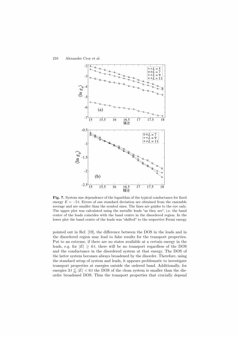
216 Alexander Croy et al.
15 15.5 16 16.5 17 17.5 18W/t
-7
-6
-5
-4
-3
-2
⟨ln
g 4⟩
L = 5L = 7L = 9L = 11
(a)
15 15.5 16 16.5 17 17.5 18W/t
-2.5
-2
-1.5
-1
-0.5
⟨ln
g4⟩
L = 7L = 9L = 11
(b)
Fig. 7. System size dependence of the logarithm of the typical conductance for fixedenergy E = −5 t. Errors of one standard deviation are obtained from the ensembleaverage and are smaller than the symbol sizes. The lines are guides to the eye only.The upper plot was calculated using the metallic leads “as they are”, i.e. the bandcentre of the leads coincides with the band centre in the disordered region. In thelower plot the band centre of the leads was “shifted” to the respective Fermi energy
pointed out in Ref. [19], the difference between the DOS in the leads and inthe disordered region may lead to false results for the transport properties.Put to an extreme, if there are no states available at a certain energy in theleads, e.g. for |E| ≥ 6 t, there will be no transport regardless of the DOSand the conductance in the disordered system at that energy. The DOS ofthe latter system becomes always broadened by the disorder. Therefore, usingthe standard setup of system and leads, it appears problematic to investigatetransport properties at energies outside the ordered band. Additionally, forenergies 3 t |E| < 6 t the DOS of the clean system is smaller than the dis-order broadened DOS. Thus the transport properties that crucially depend
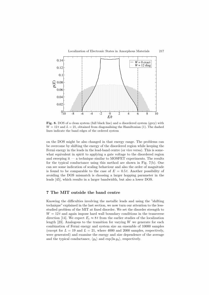
Localization of Electronic States in Amorphous Materials 217
-10 -8 -6 -4 -2 0 2 4 6 8 10E/t
0
0.02
0.04
0.06
0.08
0.1
0.12
0.14
ρ(E
)
W = 0 exactW = 12 diag
Fig. 8. DOS of a clean system (full black line) and a disordered system (grey) withW = 12 t and L = 21, obtained from diagonalising the Hamiltonian (1). The dashedlines indicate the band edges of the ordered system
on the DOS might be also changed in that energy range. The problems canbe overcome by shifting the energy of the disordered region while keeping theFermi energy in the leads in the lead-band centre (or vice versa). This is some-what equivalent in spirit to applying a gate voltage to the disordered regionand sweeping it — a technique similar to MOSFET experiments. The resultsfor the typical conductance using this method are shown in Fig. 7(b). Onecan see some indication of scaling behaviour and also the order of magnitudeis found to be comparable to the case of E = 0.5 t. Another possibility ofavoiding the DOS mismatch is choosing a larger hopping parameter in theleads [45], which results in a larger bandwidth, but also a lower DOS.
7 The MIT outside the band centre
Knowing the difficulties involving the metallic leads and using the ”shiftingtechnique” explained in the last section, we now turn our attention to the less-studied problem of the MIT at fixed disorder. We set the disorder strength toW = 12 t and again impose hard wall boundary conditions in the transversedirection [14]. We expect Ec ≈ 8 t from the earlier studies of the localizationlength [23]. Analogous to the transition for varying W we generate for eachcombination of Fermi energy and system size an ensemble of 10000 samples(except for L = 19 and L = 21, where 4000 and 2000 samples, respectively,were generated) and examine the energy and size dependence of the averageand the typical conductance, 〈g4〉 and exp〈ln g4〉, respectively.
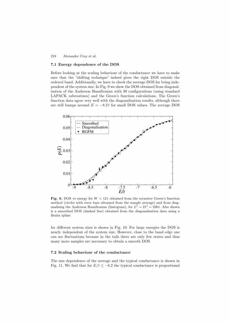
218 Alexander Croy et al.
7.1 Energy dependence of the DOS
Before looking at the scaling behaviour of the conductance we have to makesure that the ”shifting technique” indeed gives the right DOS outside theordered band. Additionally, we have to check the average DOS for being inde-pendent of the system size. In Fig. 9 we show the DOS obtained from diagonal-isation of the Anderson Hamiltonian with 30 configurations (using standardLAPACK subroutines) and the Green’s function calculations. The Green’sfunction data agree very well with the diagonalisation results, although thereare still bumps around E = −8.2 t for small DOS values. The average DOS
-9 -8.5 -8 -7.5 -7 -6.5 -6E/t
0
0.01
0.02
0.03
0.04
0.05
0.06
ρ(E
)
SmoothedDiagonalisationRGFM
Fig. 9. DOS vs energy for W = 12 t obtained from the recursive Green’s functionmethod (circles with error bars obtained from the sample average) and from diag-onalising the Anderson Hamiltonian (histogram), for L3 = 213 = 9261. Also shownis a smoothed DOS (dashed line) obtained from the diagonalisation data using aBezier spline
for different system sizes is shown in Fig. 10. For large energies the DOS isnearly independent of the system size. However, close to the band edge onecan see fluctuations because in the tails there are only few states and thusmany more samples are necessary to obtain a smooth DOS.
7.2 Scaling behaviour of the conductance
The size dependence of the average and the typical conductance is shown inFig. 11. We find that for E/t ≤ −8.2 the typical conductance is proportional
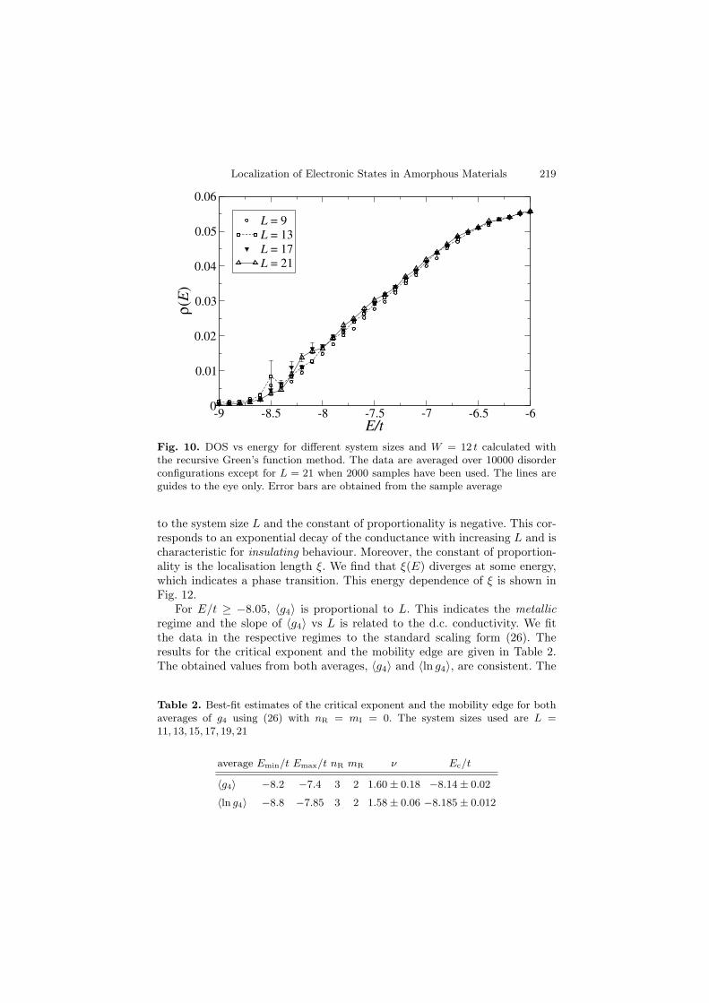
Localization of Electronic States in Amorphous Materials 219
-9 -8.5 -8 -7.5 -7 -6.5 -6E/t
0
0.01
0.02
0.03
0.04
0.05
0.06ρ
(E)
L = 9L = 13L = 17L = 21
Fig. 10. DOS vs energy for different system sizes and W = 12 t calculated withthe recursive Green’s function method. The data are averaged over 10000 disorderconfigurations except for L = 21 when 2000 samples have been used. The lines areguides to the eye only. Error bars are obtained from the sample average
to the system size L and the constant of proportionality is negative. This cor-responds to an exponential decay of the conductance with increasing L and ischaracteristic for insulating behaviour. Moreover, the constant of proportion-ality is the localisation length ξ. We find that ξ(E) diverges at some energy,which indicates a phase transition. This energy dependence of ξ is shown inFig. 12.
For E/t ≥ −8.05, 〈g4〉 is proportional to L. This indicates the metallicregime and the slope of 〈g4〉 vs L is related to the d.c. conductivity. We fitthe data in the respective regimes to the standard scaling form (26). Theresults for the critical exponent and the mobility edge are given in Table 2.The obtained values from both averages, 〈g4〉 and 〈ln g4〉, are consistent. The
Table 2. Best-fit estimates of the critical exponent and the mobility edge for bothaverages of g4 using (26) with nR = mI = 0. The system sizes used are L =11, 13, 15, 17, 19, 21
average Emin/t Emax/t nR mR ν Ec/t
〈g4〉 −8.2 −7.4 3 2 1.60 ± 0.18 −8.14 ± 0.02
〈ln g4〉 −8.8 −7.85 3 2 1.58 ± 0.06 −8.185 ± 0.012
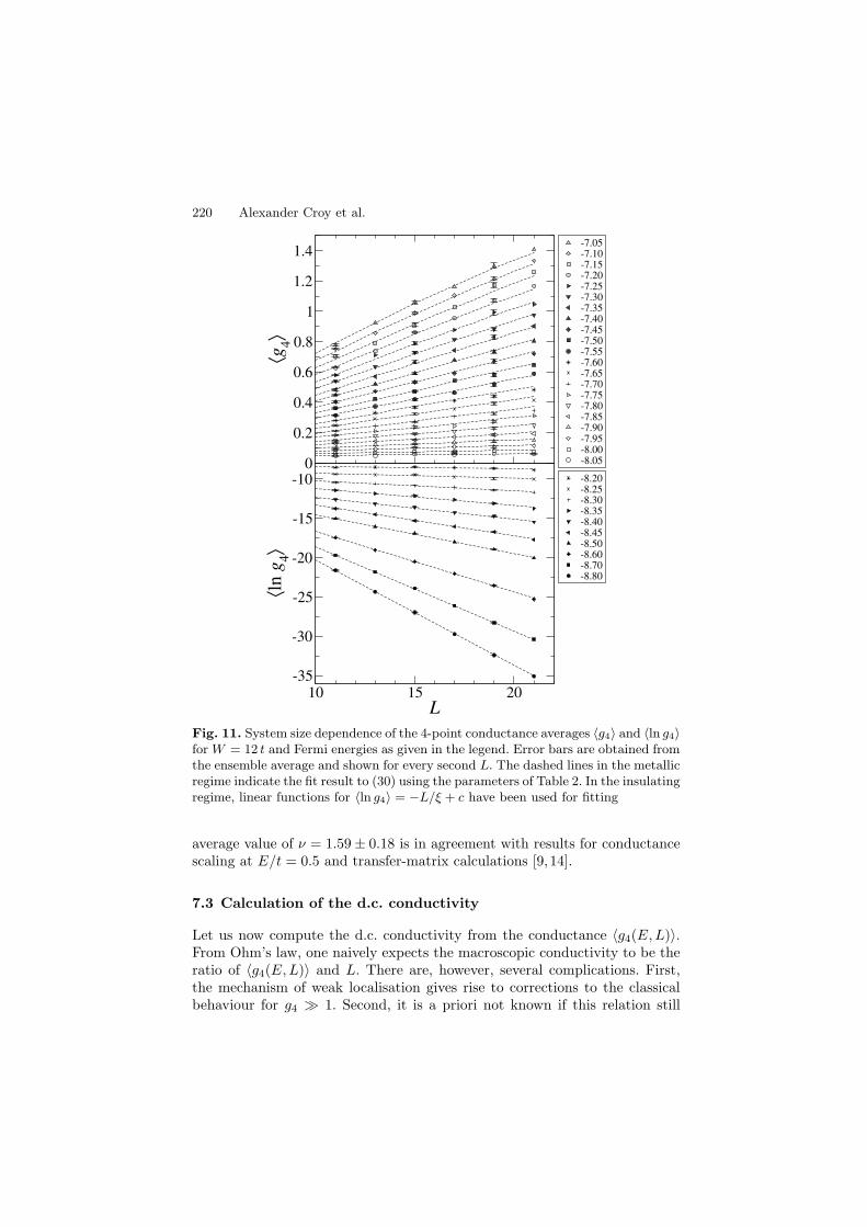
220 Alexander Croy et al.
0
0.2
0.4
0.6
0.8
1
1.2
1.4
⟨g4⟩
-7.05-7.10-7.15-7.20-7.25-7.30-7.35-7.40-7.45-7.50-7.55-7.60-7.65-7.70-7.75-7.80-7.85-7.90-7.95-8.00-8.05
10 15 20L
-35
-30
-25
-20
-15
-10
⟨ln
g 4⟩
-8.20-8.25-8.30-8.35-8.40-8.45-8.50-8.60-8.70-8.80
Fig. 11. System size dependence of the 4-point conductance averages 〈g4〉 and 〈ln g4〉for W = 12 t and Fermi energies as given in the legend. Error bars are obtained fromthe ensemble average and shown for every second L. The dashed lines in the metallicregime indicate the fit result to (30) using the parameters of Table 2. In the insulatingregime, linear functions for 〈ln g4〉 = −L/ξ + c have been used for fitting
average value of ν = 1.59± 0.18 is in agreement with results for conductancescaling at E/t = 0.5 and transfer-matrix calculations [9, 14].
7.3 Calculation of the d.c. conductivity
Let us now compute the d.c. conductivity from the conductance 〈g4(E,L)〉.From Ohm’s law, one naively expects the macroscopic conductivity to be theratio of 〈g4(E,L)〉 and L. There are, however, several complications. First,the mechanism of weak localisation gives rise to corrections to the classicalbehaviour for g4 ≫ 1. Second, it is a priori not known if this relation still
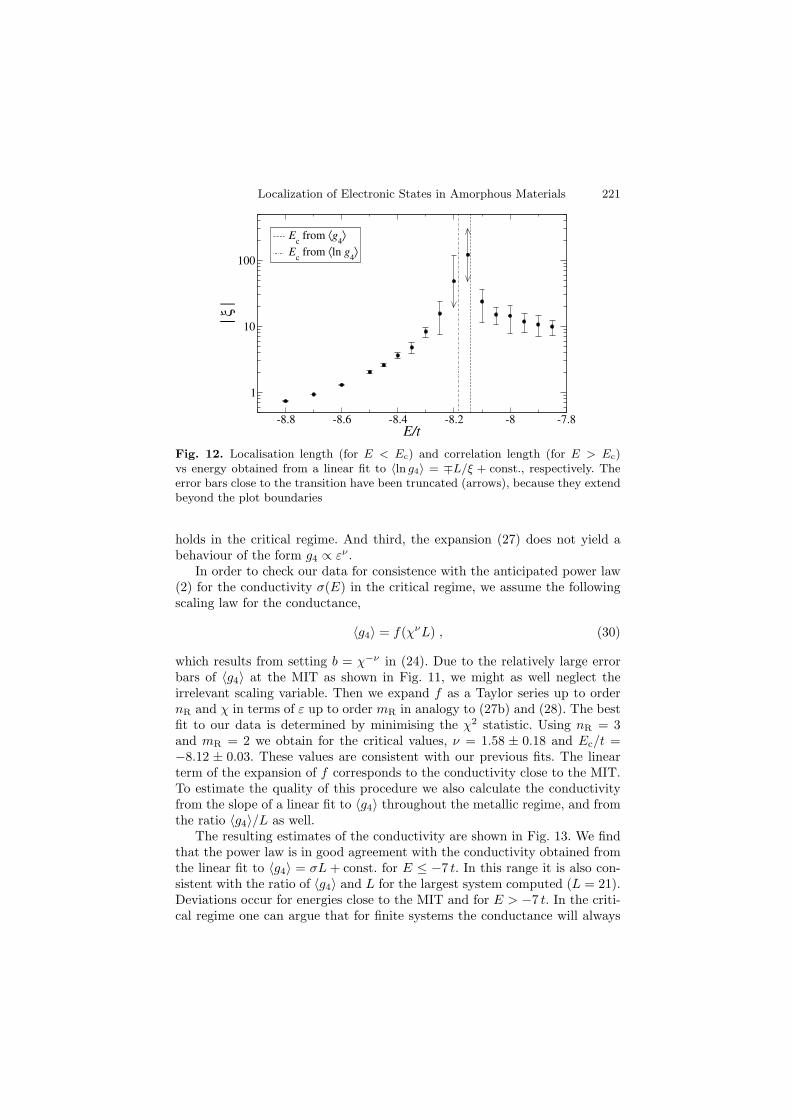
Localization of Electronic States in Amorphous Materials 221
-8.8 -8.6 -8.4 -8.2 -8 -7.8E/t
1
10
100
| ξ |
Ec from ⟨g
4⟩
Ec from ⟨ln g
4⟩
Fig. 12. Localisation length (for E < Ec) and correlation length (for E > Ec)vs energy obtained from a linear fit to 〈ln g4〉 = ∓L/ξ + const., respectively. Theerror bars close to the transition have been truncated (arrows), because they extendbeyond the plot boundaries
holds in the critical regime. And third, the expansion (27) does not yield abehaviour of the form g4 ∝ εν .
In order to check our data for consistence with the anticipated power law(2) for the conductivity σ(E) in the critical regime, we assume the followingscaling law for the conductance,
〈g4〉 = f(χνL) , (30)
which results from setting b = χ−ν in (24). Due to the relatively large errorbars of 〈g4〉 at the MIT as shown in Fig. 11, we might as well neglect theirrelevant scaling variable. Then we expand f as a Taylor series up to ordernR and χ in terms of ε up to order mR in analogy to (27b) and (28). The bestfit to our data is determined by minimising the χ2 statistic. Using nR = 3and mR = 2 we obtain for the critical values, ν = 1.58 ± 0.18 and Ec/t =−8.12 ± 0.03. These values are consistent with our previous fits. The linearterm of the expansion of f corresponds to the conductivity close to the MIT.To estimate the quality of this procedure we also calculate the conductivityfrom the slope of a linear fit to 〈g4〉 throughout the metallic regime, and fromthe ratio 〈g4〉/L as well.
The resulting estimates of the conductivity are shown in Fig. 13. We findthat the power law is in good agreement with the conductivity obtained fromthe linear fit to 〈g4〉 = σL+ const. for E ≤ −7 t. In this range it is also con-sistent with the ratio of 〈g4〉 and L for the largest system computed (L = 21).Deviations occur for energies close to the MIT and for E > −7 t. In the criti-cal regime one can argue that for finite systems the conductance will always
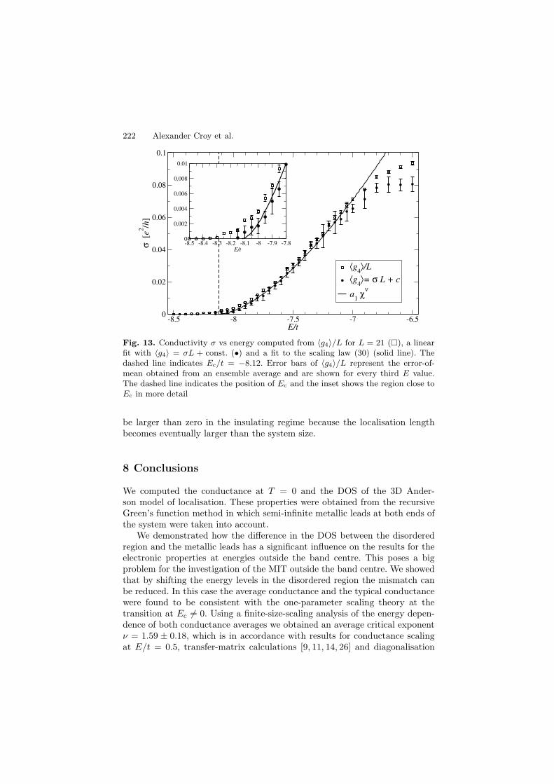
222 Alexander Croy et al.
-8.5 -8 -7.5 -7 -6.5E/t
0
0.02
0.04
0.06
0.08
0.1σ
[e
2 /h]
⟨g4⟩/L
⟨g4⟩= σ L + c
a1
χν
-8.5 -8.4 -8.3 -8.2 -8.1 -8 -7.9 -7.8E/t
0
0.002
0.004
0.006
0.008
0.01
Fig. 13. Conductivity σ vs energy computed from 〈g4〉/L for L = 21 (), a linearfit with 〈g4〉 = σL + const. (•) and a fit to the scaling law (30) (solid line). Thedashed line indicates Ec/t = −8.12. Error bars of 〈g4〉/L represent the error-of-mean obtained from an ensemble average and are shown for every third E value.The dashed line indicates the position of Ec and the inset shows the region close toEc in more detail
be larger than zero in the insulating regime because the localisation lengthbecomes eventually larger than the system size.
8 Conclusions
We computed the conductance at T = 0 and the DOS of the 3D Ander-son model of localisation. These properties were obtained from the recursiveGreen’s function method in which semi-infinite metallic leads at both ends ofthe system were taken into account.
We demonstrated how the difference in the DOS between the disorderedregion and the metallic leads has a significant influence on the results for theelectronic properties at energies outside the band centre. This poses a bigproblem for the investigation of the MIT outside the band centre. We showedthat by shifting the energy levels in the disordered region the mismatch canbe reduced. In this case the average conductance and the typical conductancewere found to be consistent with the one-parameter scaling theory at thetransition at Ec = 0. Using a finite-size-scaling analysis of the energy depen-dence of both conductance averages we obtained an average critical exponentν = 1.59 ± 0.18, which is in accordance with results for conductance scalingat E/t = 0.5, transfer-matrix calculations [9, 11, 14, 26] and diagonalisation
Localization of Electronic States in Amorphous Materials 223
studies [10,12]. However, a thorough investigation of the influence of the leadsis still lacking. It would also be interesting to see if these effects can be relatedto studies of 1D multichannel systems with impurities [46].
We calculated the d.c. conductivity from the system-size dependence ofthe average conductance and found it consistent with a power-law form atthe MIT [47]. This strongly supports previous analytical and numerical cal-culations of thermoelectric properties reviewed in Ref. [3]. Similar resultsfor topologically disordered Anderson models [48–50], random-hopping mod-els [37,51–53] and the interplay of disorder and many-body interaction [54–57]have been reported elsewhere.
Acknowledgments
We thankfully acknowledge fruitful and localized discussions with P. Cain, F.Milde, M.L. Ndawana and C. de los Reyes Villagonzalo.
References
1. P. W. Anderson. Absence of diffusion in certain random lattices. Phys. Rev.,109:1492–1505, 1958.
2. B. Kramer and A. MacKinnon. Localization: theory and experiment. Rep. Prog.Phys., 56:1469–1564, 1993.
3. R. A. Romer and M. Schreiber. Numerical investigations of scaling at the An-derson transition. In T. Brandes and S. Kettemann, editors, The AndersonTransition and its Ramifications — Localisation, Quantum Interference, andInteractions, volume 630 of Lecture Notes in Physics, pages 3–19. Springer,Berlin, 2003.
4. I. Plyushchay, R. A. Romer, and M. Schreiber. The three-dimensional Andersonmodel of localization with binary random potential. Phys. Rev. B, 68:064201,2003.
5. J. E. Enderby and A. C. Barnes. Electron transport at the Anderson transition.Phys. Rev. B, 49:5062, 1994.
6. C. Villagonzalo, R. A. Romer, and M. Schreiber. Thermoelectric transportproperties in disordered systems near the Anderson transition. Eur. Phys. J. B,12:179–189, 1999. ArXiv: cond-mat/9904362.
7. E. Abrahams, P. W. Anderson, D. C. Licciardello, and T. V. Ramakrishnan.Scaling theory of localization: absence of quantum diffusion in two dimensions.Phys. Rev. Lett., 42:673–676, 1979.
8. P. A. Lee and T. V. Ramakrishnan. Disordered electronic systems. Rev. Mod.Phys., 57:287–337, 1985.
9. K. Slevin and T. Ohtsuki. Corrections to scaling at the Anderson transition.Phys. Rev. Lett., 82:382–385, 1999. ArXiv: cond-mat/9812065.
10. F. Milde, R. A. Romer, and M. Schreiber. Energy-level statistics at the metal-insulator transition in anisotropic systems. Phys. Rev. B, 61:6028–6035, 2000.
11. F. Milde, R. A. Romer, M. Schreiber, and V. Uski. Critical properties of themetal-insulator transition in anisotropic systems. Eur. Phys. J. B, 15:685–690,2000. ArXiv: cond-mat/9911029.
224 Alexander Croy et al.
12. M. L. Ndawana, R. A. Romer, and M. Schreiber. Finite-size scaling of the levelcompressibility at the Anderson transition. Eur. Phys. J. B, 27:399–407, 2002.
13. M. L. Ndawana, R. A. Romer, and M. Schreiber. Effects of scale-free disorderon the Anderson metal-insulator transition. Europhys. Lett., 68:678–684, 2004.
14. K. Slevin, P. Markos, and T. Ohtsuki. Reconciling conductance fluctuations andthe scaling theory of localization. Phys. Rev. Lett., 86:3594–3597, 2001.
15. D. Braun, E. Hofstetter, G. Montambaux, and A. MacKinnon. Boundary con-ditions, the critical conductance distribution, and one-parameter scaling. Phys.Rev. B, 64:155107, 2001.
16. C. Villagonzalo, R. A. Romer, and M. Schreiber. Transport properties nearthe Anderson transition. Ann. Phys. (Leipzig), 8:SI-269–SI-272, 1999. ArXiv:cond-mat/9908218.
17. C. Villagonzalo, R. A. Romer, M. Schreiber, and A. MacKinnon. Behavior of thethermopower in amorphous materials at the metal-insulator transition. Phys.Rev. B, 62:16446–16452, 2000.
18. A. MacKinnon. The conductivity of the one-dimensional disordered Andersonmodel: a new numerical method. J. Phys.: Condens. Matter, 13:L1031–L1034,1980.
19. A. MacKinnon. The calculation of transport properties and density of states ofdisordered solids. Z. Phys. B, 59:385–390, 1985.
20. B. Mehlig and M. Schreiber. Energy-level and wave-function statistics in the An-derson model of localization. In K.H. Hoffmann and A. Meyer, editors, ParallelAlgorithms and Cluster Computing - Implementations, Algorithms, and Appli-cations, Lecture Notes in Computational Science and Engineering. Springer,Berlin, 2006.
21. P. Karmann, R. A. Romer, M. Schreiber, and P. Stollmann. Fine structure of theintegrated density of states for Bernoulli-Anderson models. In K.H. Hoffmann,and A. Meyer, editors, Parallel Algorithms and Cluster Computing - Implemen-tations, Algorithms, and Applications, Lecture Notes in Computational Scienceand Engineering. Springer, Berlin, 2006.
22. B. Bulka, B. Kramer, and A. MacKinnon. Mobility edge in the three dimensionalAnderson model. Z. Phys. B, 60:13–17, 1985.
23. B. Bulka, M. Schreiber, and B. Kramer. Localization, quantum interference,and the metal-insulator transition. Z. Phys. B, 66:21, 1987.
24. T. Ohtsuki, K. Slevin, and T. Kawarabayashi. Review on recent progress onnumerical studies of the Anderson transition. Ann. Phys. (Leipzig), 8:655–664,1999. ArXiv: cond-mat/9911213.
25. T. Ando. Numerical study of symmetry effects on localization in two dimensions.Phys. Rev. B, 40:5325, 1989.
26. P. Cain, R. A. Romer, and M. Schreiber. Phase diagram of the three-dimensionalAnderson model of localization with random hopping. Ann. Phys. (Leipzig),8:SI-33–SI-38, 1999. ArXiv: cond-mat/9908255.
27. F. Milde, R. A. Romer, and M. Schreiber. Multifractal analysis of the metal-insulator transition in anisotropic systems. Phys. Rev. B, 55:9463–9469, 1997.
28. H. Stupp, M. Hornung, M. Lakner, O. Madel, and H. v. Lohneysen. Possiblesolution of the conductivity exponent puzzle for the metal-insulator transition inheavily doped uncompensated semiconductors. Phys. Rev. Lett., 71:2634–2637,1993.
Localization of Electronic States in Amorphous Materials 225
29. S. Waffenschmidt, C. Pfleiderer, and H. v. Lohneysen. Critical behavior of theconductivity of Si:P at the metal-insulator transition under uniaxial stress. Phys.Rev. Lett., 83:3005–3008, 1999. ArXiv: cond-mat/9905297.
30. F. Wegner. Electrons in disordered systems. Scaling near the mobility edge. Z.Phys. B, 25:327–337, 1976.
31. D. Belitz and T. R. Kirkpatrick. The Anderson-Mott transition. Rev. Mod.Phys., 66:261–380, 1994.
32. R. A. Romer, C. Villagonzalo, and A. MacKinnon. Thermoelectric propertiesof disordered systems. J. Phys. Soc. Japan, 72:167–168, 2002. Suppl. A.
33. C. Villagonzalo. Thermoelectric Transport at the Metal-Insulator Transition inDisordered Systems. PhD thesis, Chemnitz University of Technology, 2001.
34. P. Cain, F. Milde, R.A. Romer, and M. Schreiber. Applications of cluster com-puting for the Anderson model of localization. In S.G. Pandalai, editor, RecentResearch Developments in Physics, volume 2, pages 171–184. Transworld Re-search Network, Trivandrum, India, 2001.
35. P. Cain, F. Milde, R. A. Romer, and M. Schreiber. Use of cluster computing forthe Anderson model of localization. Comp. Phys. Comm., 147:246–250, 2002.
36. B. Kramer and M. Schreiber. Transfer-matrix methods and finite-size scaling fordisordered systems. In K. H. Hoffmann and M. Schreiber, editors, ComputationalPhysics, pages 166–188, Springer, Berlin, 1996.
37. A. Eilmes, R. A. Romer, and M. Schreiber. The two-dimensional Andersonmodel of localization with random hopping. Eur. Phys. J. B, 1:29–38, 1998.
38. U. Elsner, V. Mehrmann, F. Milde, R. A. Romer, and M. Schreiber. The An-derson model of localization: a challenge for modern eigenvalue methods. SIAMJ. Sci. Comp., 20:2089–2102, 1999. ArXiv: physics/9802009.
39. M. Schreiber, F. Milde, R. A. Romer, U. Elsner, and V. Mehrmann. Elec-tronic states in the Anderson model of localization: benchmarking eigenvaluealgorithms. Comp. Phys. Comm., 121–122:517–523, 1999.
40. E. N. Economou. Green’s Functions in Quantum Physics. Springer-Verlag,Berlin, 1990.
41. G. Czycholl, B. Kramer, and A. MacKinnon. Conductivity and localization ofelectron states in one dimensional disordered systems: further numerical results.Z. Phys. B, 43:5–11, 1981.
42. J. L. Cardy. Scaling and Renormalization in Statistical Physics. CambridgeUniversity Press, Cambridge, 1996.
43. M. Buttiker. Absence of backscattering in the quantum Hall effect in multiprobeconductors. Phys. Rev. B, 38:9375, 1988.
44. A. Croy. Thermoelectric properties of disordered systems. M.Sc. thesis, Univer-sity of Warwick, Coventry, United Kindgom, 2005.
45. B. K. Nikolic. Statistical properties of eigenstates in three-dimensional meso-scopic systems with off-diagonal or diagonal disorder. Phys. Rev. B, 64:14203,2001.
46. D. Boese, M. Lischka, and L.E. Reichl. Scaling behaviour in a quantum wirewith scatterers. Phys. Rev. B, 62:16933, 2000.
47. P. Cain, M. L. Ndawana, R. A. Romer, and M. Schreiber. The critical exponentof the localization length at the Anderson transition in 3D disordered systemsis larger than 1. 2001. ArXiv: cond-mat/0106005.
48. J. X. Zhong, U. Grimm, R. A. Romer, and M. Schreiber. Level spacing distrib-utions of planar quasiperiodic tight-binding models. Phys. Rev. Lett., 80:3996–3999, 1998.
226 Alexander Croy et al.
49. U. Grimm, R. A. Romer, and G. Schliecker. Electronic states in topologicallydisordered systems. Ann. Phys. (Leipzig), 7:389–393, 1998.
50. U. Grimm, R. A. Romer, M. Schreiber, and J. X. Zhong. Universal level-spacingstatistics in quasiperiodic tight-binding models. Mat. Sci. Eng. A, 294-296:564,2000. ArXiv: cond-mat/9908063.
51. A. Eilmes, R. A. Romer, and M. Schreiber. Critical behavior in the two-dimensional Anderson model of localization with random hopping. phys. stat.sol. (b), 205:229–232, 1998.
52. P. Biswas, P. Cain, R. A. Romer, and M. Schreiber. Off-diagonal disorder in theAnderson model of localization. phys. stat. sol. (b), 218:205–209, 2000. ArXiv:cond-mat/0001315.
53. A. Eilmes, R. A. Romer, and M. Schreiber. Localization properties of two inter-acting particles in a quasi-periodic potential with a metal-insulator transition.Eur. Phys. J. B, 23:229–234, 2001. ArXiv: cond-mat/0106603.
54. R. A. Romer and A. Punnoose. Enhanced charge and spin currents in the one-dimensional disordered mesoscopic Hubbard ring. Phys. Rev. B, 52:14809–14817,1995.
55. M. Leadbeater, R. A. Romer, and M. Schreiber. Interaction-dependent enhance-ment of the localisation length for two interacting particles in a one-dimensionalrandom potential. Eur. Phys. J. B, 8:643–652, 1999.
56. R. A. Romer, M. Schreiber, and T. Vojta. Disorder and two-particle interactionin low-dimensional quantum systems. Physica E, 9:397–404, 2001.
57. C. Schuster, R. A. Romer, and M. Schreiber. Interacting particles at a metal-insulator transition. Phys. Rev. B, 65:115114–7, 2002.
Optimizing Simulated Annealing Schedulesfor Amorphous Carbons
Peter Blaudeck and Karl Heinz Hoffmann
Technische Universitat Chemnitz, Institut fur Physik09107 Chemnitz, [email protected]
1 Introduction
Annealing, carried out in simulation, has taken on an existence of its own asa tool to solve optimization problems of many kinds [1–3]. One of many im-portant applications is to find local minima for the potential energy of atomicstructures, as in this paper, in particular structures of amorphous carbon atroom temperature. Carbon is one of the most promising chemical elements formolecular structure design in nature. An infinite richness of different struc-tures with an incredibly wide variety of physical properties can be produced.Apart from the huge variety of organic substances, even the two crystallineinorganic modifications, graphite and diamond, show diametrically oppositephysical properties. Amorphous carbon continues to attract researchers forboth the fundamental understanding of the microstructure and stability ofthe material and the increasing interest in various applications as a high per-formance coating material as well as in electronic devices.
Simulated Annealing (SA) of such systems requires to apply methods ofmolecular dynamics (MD) to the ensemble of atoms [4]. The first fundamentalstep is to find a suitable approach to the interatomic potentials and forces. Inthe spectrum of useful methods there are on the one hand the empirical po-tential models, for example the Tersoff potential [5]. These are simple enoughto allow computations with many thousands of atoms but are limited in ac-curacy and chemical transferability to situations, that have not been includedin the parametrization. On the other hand, fully self-consistent quantum me-chanical approaches for general structures of any kind of atoms [6,7] are, dueto their complexity, limited to short time simulations of only about one hun-dred atoms. The method used in this paper [8] takes an intermediate positionbetween the empirical and the ab initio approaches and is briefly outlined inSect. 2.
In Sect. 3 we give a short description of how to use parallel computation toovercome the general problem of the limited computer power by optimizingand performing SA schedules for any given computational resource and, in
228 Peter Blaudeck and Karl Heinz Hoffmann
principle, for any finite system of atoms or molecules. Finally, an example ofthe effect of the optimization is shown in Sect. 4, using the new optimizedschedule and comparing its results with old data.
2 Density-functional molecular dynamics
We apply the well established ab initio based non-selfconsistent tight-bindingscheme [8], which, compared with fully self–consistent calculations, reduces thecomputational effort by at least two orders of magnitude. The approximatecalculation of the MD interatomic forces is based on the density functionaltheory (DFT) within the local density approximation (LDA) using a localizedatomic orbital (LCAO) basis [9]. The scheme includes first-principle conceptsin relating the Kohn-Sham orbitals of the many-atom configuration to a mini-mal basis of the localized atomic-like valence orbitals of all atoms. We take intoaccount only two-center Hamiltonian matrix elements h and overlap matrixelements S in the secular equation resulting in a general eigenvalue problem
∑
µ
ciµ(hµν − ǫiSµν) = 0 (1)
for the eigenvalues ǫi and eigenfunctions ciµ of the system [10]. The totalpotential energy of the system as a function of the atomic coordinates Rlcan now be decomposed into two parts,
Epot(Rl) = Ebind(Rl) + Erep(Rl −Rk). (2)
The first term Ebind is the sum of all occupied cluster electronic energies andrepresents the so-called band-structure energy. The second term, as a repul-sive energy Erep, comprises the core-core repulsion between the atoms andcorrections due to the Hartree double-counting terms and the non-linearity inthe superposition of exchange-correlation contributions. This term is fitted tothe two-particle self-consistent LDA cohesive energy curves of correspondingdiatomic molecules and crystalline modifications [11].
To apply the scheme to a part of an infinite system we carry out thesimulation for a number of atoms in a fixed-volume cubic supercell using peri-odic boundary conditions. Furthermore, the temperature has to be controlledaccording to a proper function T (t). To adjust the temperature, all atomicvelocities are renormalized after a time step to achieve the correct mean ki-netic energy per degree of freedom. The so defined temperature as a functionof time has to follow the SA schedule.
A generally unsolved problem in any high performance computation fordensity-functional based or fully self-consistently SA of real material prob-lems is, also in making use of the fastest computers, that it is only possibleto simulate the annealing of 100 or 1000 atoms for timescales of just some
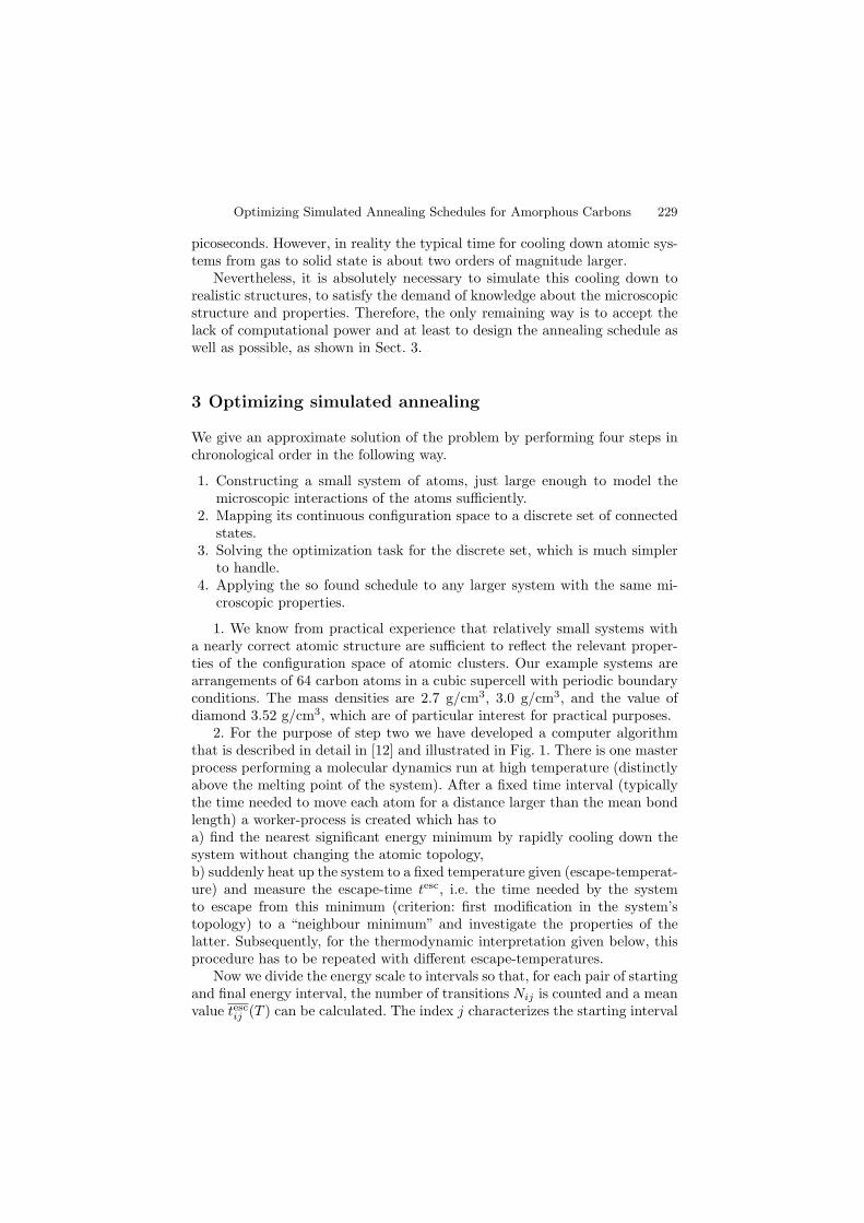
Optimizing Simulated Annealing Schedules for Amorphous Carbons 229
picoseconds. However, in reality the typical time for cooling down atomic sys-tems from gas to solid state is about two orders of magnitude larger.
Nevertheless, it is absolutely necessary to simulate this cooling down torealistic structures, to satisfy the demand of knowledge about the microscopicstructure and properties. Therefore, the only remaining way is to accept thelack of computational power and at least to design the annealing schedule aswell as possible, as shown in Sect. 3.
3 Optimizing simulated annealing
We give an approximate solution of the problem by performing four steps inchronological order in the following way.
1. Constructing a small system of atoms, just large enough to model themicroscopic interactions of the atoms sufficiently.
2. Mapping its continuous configuration space to a discrete set of connectedstates.
3. Solving the optimization task for the discrete set, which is much simplerto handle.
4. Applying the so found schedule to any larger system with the same mi-croscopic properties.
1. We know from practical experience that relatively small systems witha nearly correct atomic structure are sufficient to reflect the relevant proper-ties of the configuration space of atomic clusters. Our example systems arearrangements of 64 carbon atoms in a cubic supercell with periodic boundaryconditions. The mass densities are 2.7 g/cm3, 3.0 g/cm3, and the value ofdiamond 3.52 g/cm3, which are of particular interest for practical purposes.
2. For the purpose of step two we have developed a computer algorithmthat is described in detail in [12] and illustrated in Fig. 1. There is one masterprocess performing a molecular dynamics run at high temperature (distinctlyabove the melting point of the system). After a fixed time interval (typicallythe time needed to move each atom for a distance larger than the mean bondlength) a worker-process is created which has toa) find the nearest significant energy minimum by rapidly cooling down thesystem without changing the atomic topology,b) suddenly heat up the system to a fixed temperature given (escape-temperat-ure) and measure the escape-time tesc, i.e. the time needed by the systemto escape from this minimum (criterion: first modification in the system’stopology) to a “neighbour minimum” and investigate the properties of thelatter. Subsequently, for the thermodynamic interpretation given below, thisprocedure has to be repeated with different escape-temperatures.
Now we divide the energy scale to intervals so that, for each pair of startingand final energy interval, the number of transitions Nij is counted and a meanvalue tescij (T ) can be calculated. The index j characterizes the starting interval
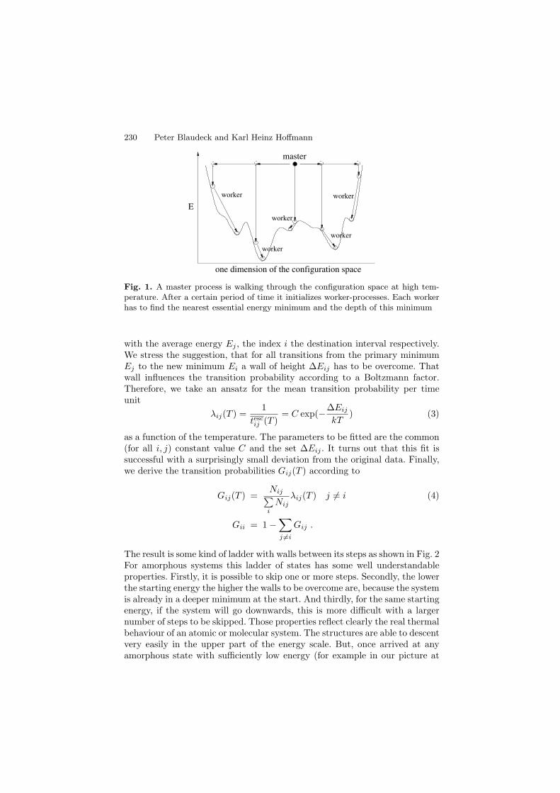
230 Peter Blaudeck and Karl Heinz Hoffmann
E
one dimension of the configuration space
master
worker
worker
worker
worker
worker
Fig. 1. A master process is walking through the configuration space at high tem-perature. After a certain period of time it initializes worker-processes. Each workerhas to find the nearest essential energy minimum and the depth of this minimum
with the average energy Ej , the index i the destination interval respectively.We stress the suggestion, that for all transitions from the primary minimumEj to the new minimum Ei a wall of height ∆Eij has to be overcome. Thatwall influences the transition probability according to a Boltzmann factor.Therefore, we take an ansatz for the mean transition probability per timeunit
λij(T ) =1
tescij (T )= C exp(−∆Eij
kT) (3)
as a function of the temperature. The parameters to be fitted are the common(for all i, j) constant value C and the set ∆Eij . It turns out that this fit issuccessful with a surprisingly small deviation from the original data. Finally,we derive the transition probabilities Gij(T ) according to
Gij(T ) =Nij∑i
Nijλij(T ) j = i (4)
Gii = 1−∑
j =i
Gij .
The result is some kind of ladder with walls between its steps as shown in Fig. 2For amorphous systems this ladder of states has some well understandableproperties. Firstly, it is possible to skip one or more steps. Secondly, the lowerthe starting energy the higher the walls to be overcome are, because the systemis already in a deeper minimum at the start. And thirdly, for the same startingenergy, if the system will go downwards, this is more difficult with a largernumber of steps to be skipped. Those properties reflect clearly the real thermalbehaviour of an atomic or molecular system. The structures are able to descentvery easily in the upper part of the energy scale. But, once arrived at anyamorphous state with sufficiently low energy (for example in our picture at
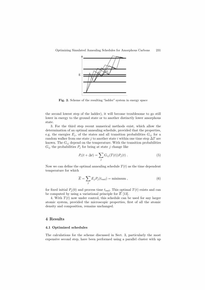
Optimizing Simulated Annealing Schedules for Amorphous Carbons 231
E
Fig. 2. Scheme of the resulting “ladder” system in energy space
the second lowest step of the ladder), it will become troublesome to go stilllower in energy to the ground state or to another distinctly lower amorphousstate.
3. For the third step recent numerical methods exist, which allow thedetermination of an optimal annealing schedule, provided that the properties,e.g. the energies Ej , of the states and all transition probabilities Gij for arandom walker from one state j to another state i within one time step ∆T areknown. The Gij depend on the temperature. With the transition probabilitiesGij the probabilities Pj for being at state j change like
Pi(t+ ∆t) =∑
j
Gij(T (t))Pj(t) . (5)
Now we can define the optimal annealing schedule T (t) as the time dependenttemperature for which
E =∑
j
EjPj(tend) = minimum , (6)
for fixed initial Pj(0) and process time tend. This optimal T (t) exists and canbe computed by using a variational principle for E [13].
4. With T (t) now under control, this schedule can be used for any largeratomic system, provided the microscopic properties, first of all the atomicdensity and composition, remains unchanged.
4 Results
4.1 Optimized schedules
The calculations for the scheme discussed in Sect. 3, particularly the mostexpensive second step, have been performed using a parallel cluster with up
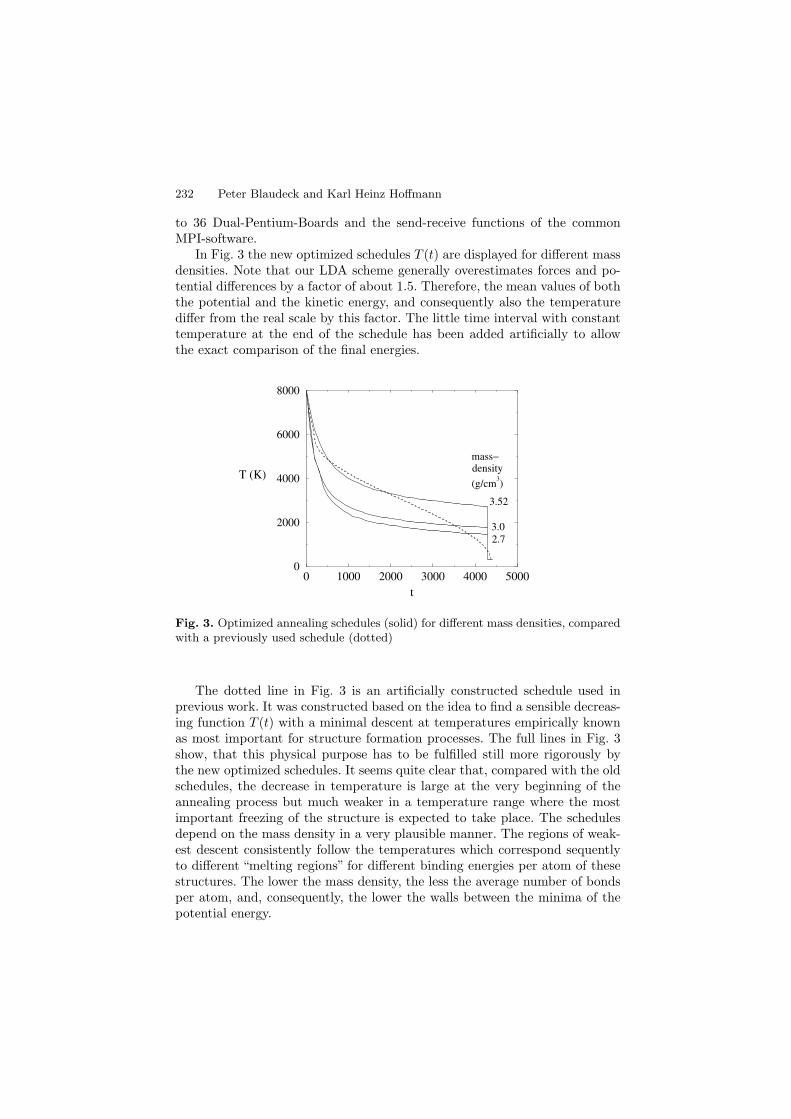
232 Peter Blaudeck and Karl Heinz Hoffmann
to 36 Dual-Pentium-Boards and the send-receive functions of the commonMPI-software.
In Fig. 3 the new optimized schedules T (t) are displayed for different massdensities. Note that our LDA scheme generally overestimates forces and po-tential differences by a factor of about 1.5. Therefore, the mean values of boththe potential and the kinetic energy, and consequently also the temperaturediffer from the real scale by this factor. The little time interval with constanttemperature at the end of the schedule has been added artificially to allowthe exact comparison of the final energies.
0 1000 2000 3000 4000 5000
t
0
2000
4000
6000
8000
T (K)
3.52
3.02.7
mass−density
(g/cm3)
Fig. 3. Optimized annealing schedules (solid) for different mass densities, comparedwith a previously used schedule (dotted)
The dotted line in Fig. 3 is an artificially constructed schedule used inprevious work. It was constructed based on the idea to find a sensible decreas-ing function T (t) with a minimal descent at temperatures empirically knownas most important for structure formation processes. The full lines in Fig. 3show, that this physical purpose has to be fulfilled still more rigorously bythe new optimized schedules. It seems quite clear that, compared with the oldschedules, the decrease in temperature is large at the very beginning of theannealing process but much weaker in a temperature range where the mostimportant freezing of the structure is expected to take place. The schedulesdepend on the mass density in a very plausible manner. The regions of weak-est descent consistently follow the temperatures which correspond sequentlyto different “melting regions” for different binding energies per atom of thesestructures. The lower the mass density, the less the average number of bondsper atom, and, consequently, the lower the walls between the minima of thepotential energy.
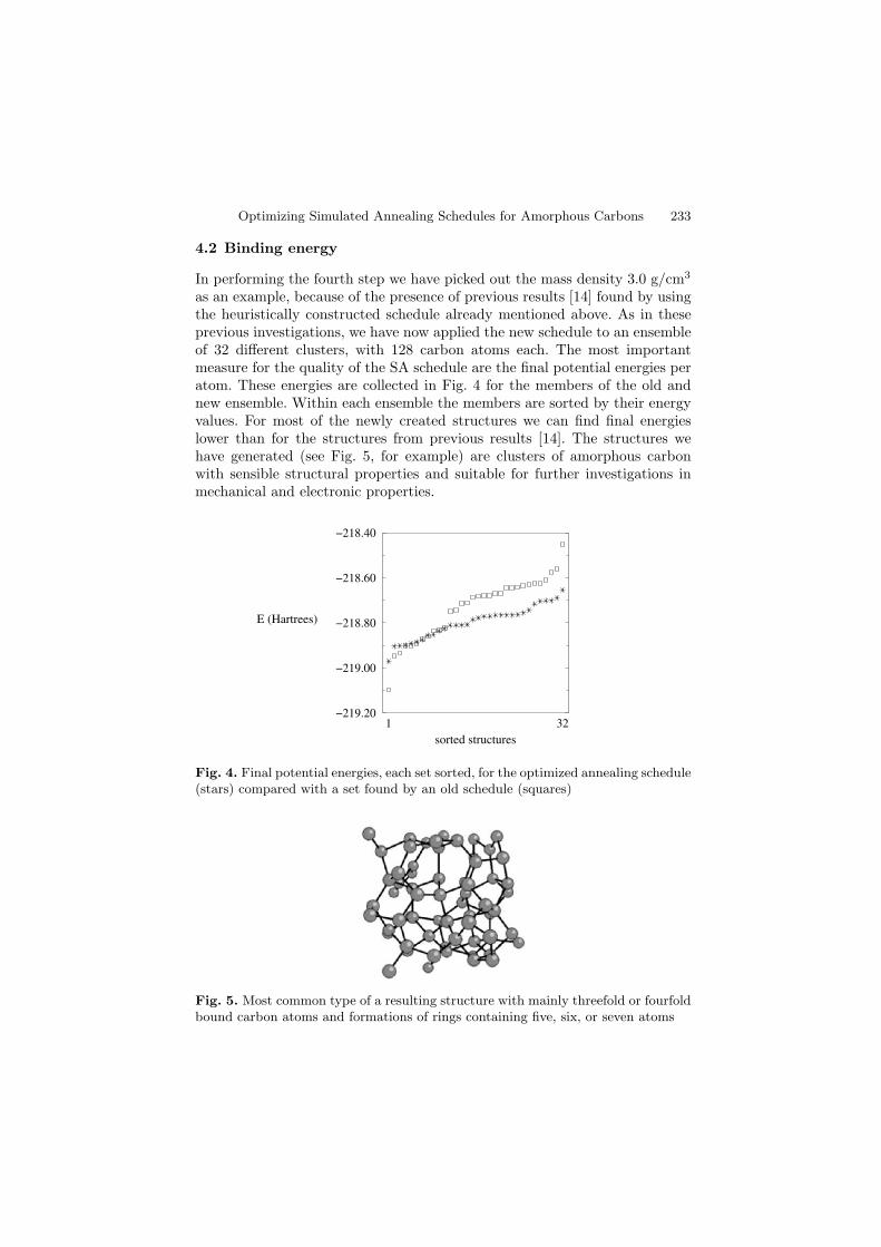
Optimizing Simulated Annealing Schedules for Amorphous Carbons 233
4.2 Binding energy
In performing the fourth step we have picked out the mass density 3.0 g/cm3
as an example, because of the presence of previous results [14] found by usingthe heuristically constructed schedule already mentioned above. As in theseprevious investigations, we have now applied the new schedule to an ensembleof 32 different clusters, with 128 carbon atoms each. The most importantmeasure for the quality of the SA schedule are the final potential energies peratom. These energies are collected in Fig. 4 for the members of the old andnew ensemble. Within each ensemble the members are sorted by their energyvalues. For most of the newly created structures we can find final energieslower than for the structures from previous results [14]. The structures wehave generated (see Fig. 5, for example) are clusters of amorphous carbonwith sensible structural properties and suitable for further investigations inmechanical and electronic properties.
1 32
sorted structures
−219.20
−219.00
−218.80
−218.60
−218.40
E (Hartrees)
Fig. 4. Final potential energies, each set sorted, for the optimized annealing schedule(stars) compared with a set found by an old schedule (squares)
Fig. 5. Most common type of a resulting structure with mainly threefold or fourfoldbound carbon atoms and formations of rings containing five, six, or seven atoms
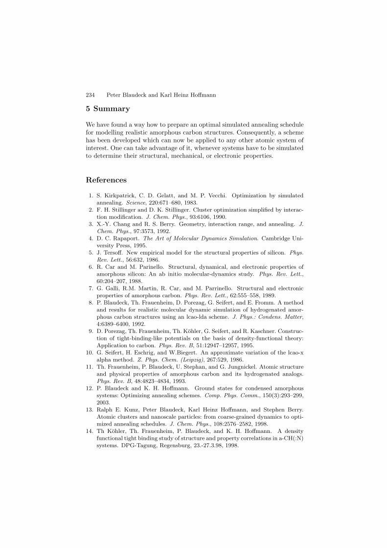
234 Peter Blaudeck and Karl Heinz Hoffmann
5 Summary
We have found a way how to prepare an optimal simulated annealing schedulefor modelling realistic amorphous carbon structures. Consequently, a schemehas been developed which can now be applied to any other atomic system ofinterest. One can take advantage of it, whenever systems have to be simulatedto determine their structural, mechanical, or electronic properties.
References
1. S. Kirkpatrick, C. D. Gelatt, and M. P. Vecchi. Optimization by simulatedannealing. Science, 220:671–680, 1983.
2. F. H. Stillinger and D. K. Stillinger. Cluster optimization simplified by interac-tion modification. J. Chem. Phys., 93:6106, 1990.
3. X.-Y. Chang and R. S. Berry. Geometry, interaction range, and annealing. J.Chem. Phys., 97:3573, 1992.
4. D. C. Rapaport. The Art of Molecular Dynamics Simulation. Cambridge Uni-versity Press, 1995.
5. J. Tersoff. New empirical model for the structural properties of silicon. Phys.Rev. Lett., 56:632, 1986.
6. R. Car and M. Parinello. Structural, dynamical, and electronic properties ofamorphous silicon: An ab initio molecular-dynamics study. Phys. Rev. Lett.,60:204–207, 1988.
7. G. Galli, R.M. Martin, R. Car, and M. Parrinello. Structural and electronicproperties of amorphous carbon. Phys. Rev. Lett., 62:555–558, 1989.
8. P. Blaudeck, Th. Frauenheim, D. Porezag, G. Seifert, and E. Fromm. A methodand results for realistic molecular dynamic simulation of hydrogenated amor-phous carbon structures using an lcao-lda scheme. J. Phys.: Condens. Matter,4:6389–6400, 1992.
9. D. Porezag, Th. Frauenheim, Th. Kohler, G. Seifert, and R. Kaschner. Construc-tion of tight-binding-like potentials on the basis of density-functional theory:Application to carbon. Phys. Rev. B, 51:12947–12957, 1995.
10. G. Seifert, H. Eschrig, and W.Biegert. An approximate variation of the lcao-xalpha method. Z. Phys. Chem. (Leipzig), 267:529, 1986.
11. Th. Frauenheim, P. Blaudeck, U. Stephan, and G. Jungnickel. Atomic structureand physical properties of amorphous carbon and its hydrogenated analogs.Phys. Rev. B, 48:4823–4834, 1993.
12. P. Blaudeck and K. H. Hoffmann. Ground states for condensed amorphoussystems: Optimizing annealing schemes. Comp. Phys. Comm., 150(3):293–299,2003.
13. Ralph E. Kunz, Peter Blaudeck, Karl Heinz Hoffmann, and Stephen Berry.Atomic clusters and nanoscale particles: from coarse-grained dynamics to opti-mized annealing schedules. J. Chem. Phys., 108:2576–2582, 1998.
14. Th Kohler, Th. Frauenheim, P. Blaudeck, and K. H. Hoffmann. A densityfunctional tight binding study of structure and property correlations in a-CH(:N)systems. DPG-Tagung, Regensburg, 23.-27.3.98, 1998.
Amorphisation at Heterophase Interfaces
Sibylle Gemming1,2, Andrey Enyashin1,3, and Michael Schreiber1
1 Technische Universitat Chemnitz, Institut fur Physik, 09107 Chemnitz, [email protected]
[email protected] Forschungszentrun Rossendorf, P.O. 51 01 19, 01314 Dresden, Germany3 Technische Universitat Dresden, Fachbereich Chemie, 01062 Dresden, [email protected]
1 Reactive heterophase interfaces
Heterophase interfaces are boundaries, which join two material types withdifferent physical and chemical nature. Therefore, heterophase interfaces canexhibit a large variety of geometric morphologies ranging from atomicallysharp boundaries to gradient materials, in which an interface-specific phaseis formed, which provides a continuous change of the structural parametersand thus reduces elastic strains and deformations. In addition, also the elec-tronic properties of the two materials may be different, e.g. at boundariesbetween an electronically conducting metal and a semiconductor or an in-sulating material. Due to the deviations in the electronic structure, variousbonding mechanisms are observed, which span the range from weakly inter-acting systems to boundaries with strong, directed bonding and further toreactively bonding systems which exhibit a new phase at the interface. Thus,both elastic and electronic factors may contribute to the formation of a new,often amorphous phase at the interface. Numerical simulations based on elec-tronic structure theory are an efficient tool to distinguish and quantify thesedifferent influence factors, and massively parallel computers nowadays providethe required numerical power to tackle structurally more demanding systems.Here, this power has been exploited by the parallelisation over an optimisedset of integration points, which split the solution of the Kohn-Sham equationsinto a set of matrix equations with equal matrix sizes. In this way, the analysisand prediction of material properties at the nanoscale has become feasible.
1.1 Structure and stability of heterophase interfaces
Junctions between two different metals or semiconductors or insulators alsobelong to the class of heterophase interfaces and have been studied to elu-cidate the influence of more subtle differences of the electronic structure.
236 Sibylle Gemming et al.
The observation of the giant magnetoresistance, for instance, has excited sev-eral theoretical investigations on metallic multilayers [1], such as Ni|Ru [2],Pt|Ta [3], Cu|Ta [4], or Ag|Pt [5]. Another active field of research are the phe-nomena related to the quantised conductance in mixed-metal nanostructuresfrom materials such as AuPd or AuAg [6–8]. Hetero- and superstructures ofIII-V and II-VI semiconductors provide the possibility to generate specific op-tical properties by adjusting the electronic and elastic properties via the layerthickness and composition, e.g. the III-V combinations GaAs|AlAs [9, 10],GaSb|InAs [10], or InAs|GaSb [11], and mixed multilayers of III-V and II-VI semiconductors like GaAs|ZnSe [12], or of III-V on IV materials, such asSiC|AlN and SiC|BP [13]. In these and other more covalently bonded systems,like SiC|Si [14], the main focus of the investigations is on the correlation oflattice strain and electronic properties. Other insulator-insulator boundariescome from the heteroepitaxy of ferroic oxides on an oxide template, such asSrTiO3|MgO [15], or multilayers such as BaTiO3|SrTiO3 [16], or from thedoping of homophase boundaries with electronically active elements, such asFe at the Σ3(111)[1-10] boundary in SrTiO3 [17, 18].
The present discussion will focus on contacts between a metal and anon-metallic material, where the electronic structures of the components dif-fer most strongly, and an electronic structure theory can best exploit itsmodelling power. Nevertheless, it has demonstrated its applicability also forsemiconductor-insulator boundaries such as C|Si [19], Si|SiO2 [20], TiN|MgO[21], or ZrO2|Si and ZrSiO4|Si [22].
1.2 Interactions at heterophase interfaces
A strong interest in a theory-based microscopic understanding of the interac-tions at metal-insulator interfaces has developed over the last decades, moti-vated by the application of ceramic materials in various industrial applications,for instance as thermal barrier coatings [23], or even as medical implants [24].The motivation to study metal-semiconductor interfaces stems mostly fromthe further miniaturisation of microelectronic devices and the concomitantneed to control interface properties between the semiconductor substrate andmetallic functional layers or the metallisation at the nanoscale.
This interest has lead to various attempts for theoretical modelling of therelevant contributions which influence the bonding behaviour at the interface.Theoretical studies span the whole range from finite-element modelling tounderstand macroscopic elastic properties [25], over atomistic simulations ofdislocation networks, plasticity, and fracture [26], to the investigation of theelectronic structure with ab-initio band-structure techniques [27–32].
From the theoretical modelling and the experimental observations onmetal-to-non-metal bonding at flat, atomically abrupt interfaces three sce-narios can be distinguished:
(A) Strong adhesion, which is for instance found for main-group or earlytransition metals on oxide-based insulators with a propensity of the metal to
Amorphisation at Heterophase Interfaces 237
bind on top of the O atom. This behaviour is, for instance, observed for Tion MgO(100) [33], for Al on Al2O3(000.1) [34], for V on MgO(001) [35], andfor Al and Ti on MgAl2O4(001) [37–42]. At reactive interfaces, such as metal-silicon contacts, the interaction between the two constituents is even larger,leading to a thermodynamic driving force for the formation of the interfacephase.
(B) Weak adhesion is obtained for late transition metals at non-polar insu-lator surfaces for instance for Ag|MgO(001) [33,43,44], for Cu|MgO(001) [26],for the VOx|Pd(111) interface [45], or for Ag|MgAl2O4(001) [37,39,42]. Due tothe also experimentally apparent lack of strong bonding [46], the underlyingadhesion mechanism has been ascribed to image charge interactions [47–51].
(C) A moderately strong bonding is obtained, when additional elastic inter-actions interfere with the metal-to-oxygen bonding. For the adhesion of Cu onthe polar (111) surface of MgO, however, evidence for a direct metal-oxygeninteraction was given and the occurrence of metal-induced gap states waspostulated [52]. Presently, transition-metal oxides such as BaTiO3, SrTiO3,or ZnO are studied as substrates for the adhesion of transition metals like Pd,Pt, or Mo [53, 54]. In contrast, at reactive interfaces the elastic interactiondoes not lead to a weakening of the interface, but rather assists the formationof the interface-specific phase, e.g. by the introduction of misfit dislocationsat the boundary.
Similar adhesive interactions are also monitored for metal-insulator con-tacts, where the insulator is not an oxide, but a carbide [55,56] or nitride [57].
2 Modelling reactive interfaces
2.1 Macroscopic modelling
From a phenomenological point of view, the three adhesion regimes can becharacterised by the growth mode during metal deposition and by the so-called wetting angle. If a metal droplet is deposited on an unreactive insulatorsurface, the balance of three major energy contributions determine its shape:the interface energy γmet−ins at the contact area of the two materials, and thetwo surface energies of insulator γins and metal γmet in contact with the envi-ronment (e.g. air). The relation between these quantities is given by Young’sequation [58]:
γins − γmet−ins = γmet cos(θ). (1)
In this equation, θ is the “contact” or “wetting” angle, which is the inclinationangle between the metal surface and the metal-insulator contact area at thetriple line between metal, insulator and air. If the interface is more stable thanthe sum of the two relaxed free surfaces, complete wetting of the ceramic bya (thin) metal film is achieved, and the wetting angle tends to zero. In thiscase, the metal can be deposited in a layer-by-layer or Franck-van-der-Merwegrowth mode. On the other hand, if the free surfaces are more stable than the
238 Sibylle Gemming et al.
interface, the metal will form (nearly spherical) droplets and thus minimisethe area of the unfavourable interface with the insulator surface. The wettingangle will approach 180, and a Volmer-Weber island growth is obtained.
In the case of reactive wetting, additional factors come into play as out-lined in detail in [58]. The most important factors are the diffusion of elementsand the formation of additional phases at the metal-insulator interface andon the metal and insulator surfaces. This phenomenon can even lead to theformation of a rim at the triple line, where the metal partially dissolves theinsulator underneath the droplet and diffusion above the insulator surface ac-cumulates material on the other side of the triple line. Also, grain-boundarygrooving has been observed below the metal droplet, where the metal preferen-tially dissolves material at boundaries (defects) of the substrate. Close to thewetting-dewetting transition point with θ ≈ 90, the growth mode dependsvery sensitively on the deposition conditions. Experimentally, it is difficult todistinguish this phenomenon from the stress-driven mixed-mode growth of is-lands on a thin wetting layer (Stranski-Krastanov growth) [59], but electronicstructure theory is particularly well suited to elucidate and quantify the differ-ent contributions. Thus, the basic features of electronic structure theory willshortly be summarised in the following. More details on mesoscopic modellingis provided e.g. by Stoneham and Harding [60] or in a recent textbook byFinnis [61].
2.2 Density-functional-based modelling
Density-functional theory (DFT) has proven an extremely efficient approachto obtain the properties of a given model system in its electronic ground state.A more detailed introduction to DFT and its extensions to non-equilibriumsystems is given in review articles such as [62–64] or textbooks such as [65,66].
Generically, the parameter-free or “ab-initio” quantum-mechanical treat-ment of the electronic properties of a system employs a wave function |Ψ〉to represent all relevant electronic degrees of freedom. This wave functiondepends on the spatial variables of all interacting particles, thus computa-tions involving the wave function become rather demanding with increasingsystem size. As shown by Hohenberg and Kohn [67], in DFT the relevant in-teraction terms can be expressed as functionals of the electron density, whichis a function of only three spatial variables. Based on the two Hohenberg-Kohn theorems, the ground state electron density can be obtained from theminimisation of the total energy functional, and all properties derived fromthis density can accordingly be calculated. In the original work these the-orems were proven only under specific constraints, which were later allevi-ated by Levy [68]. Other generalisations were introduced for spin-polarisedsystems [69], for systems at finite temperature [70], and for relativistic sys-tems [71,72]. Furthermore, most electronic structure calculations make use ofthe Kohn-Sham formalism, in which the original density-based functional isre-expressed in a basis of non-interacting single-particle states. The resulting
Amorphisation at Heterophase Interfaces 239
matrix equation is a generalised eigenvalue problem, the solution of whichyields the ground-state single-particle energies. Excitation spectra have alsobecome accessible by time-dependent DFT and Bethe-Salpeter formalisms;detailed descriptions of those developments are available in [64,65].
2.3 Approximative modelling methods
Routine applications of full DFT schemes comprise model systems with upto a few hundreds of atoms. Larger systems of up to several thousands ofatoms are still tractable with approximations to the full DFT methods, suchas the tight-binding (TB) description. The standard TB method also relieson a valence-only treatment, in which the electronic valence states are repre-sented as a symmetry-adapted superposition of atomic orbitals. The Hamiltonoperator of the full Kohn-Sham formalism is approximated by a parametrisedHamiltonian, whose matrix elements are fitted to the properties of referencesystems. A short-range repulsive potential includes the ionic repulsion andcorrections due to approximations made in the band-structure term. It canbe determined as a parametrised function of the interatomic distance, whichreproduces the cohesive energy and elastic constants like the bulk modulusfor crystalline systems.
Although the results of a TB calculation depend on the parametrisation,successful applications include high accuracy band structure evaluations ofbulk semiconductors [73], band calculations in semiconductor heterostruc-tures [74], device simulations for optical properties [75], simulations of amor-phous solids [76], and predictions of low-energy silicon clusters [77, 78] (fora review, see [79]). Due to the simple parametrisation, the TB methods al-low routine calculations with up to 1000 to 2000 atoms. Thus they allow anextension to more irregular interface structures, which have a larger repeatunit, and a more detailed assessment of the energy landscape, which includesa larger number of structure models. Another advantage is the simple deriva-tion of additional quantities from TB data, because the TB approximationsalso simplify the mathematical effort for the calculation of material proper-ties. Even the transport in a nanodevice of conducting and semiconductingsegments along a nanotube could be modelled within a Landauer-Buttikerapproach [80].
2.4 Efficient parallel computing for material properties
In the ground-state electronic-structure treatment the translational symme-try of a regular crystalline solid can be exploited. Only a small unit cell ofthe whole crystal is calculated explicitly, and the properties of the extendedcrystal are retrieved by applying periodic boundary conditions in three dimen-sions. The lattice periodicity suggests plane waves as an optimal basis for therepresentation of the electronic states. However, the strongly localised innercore electrons, such as 1s states of Mg or Al, require a very high number of
240 Sibylle Gemming et al.
plane waves (or kinetic energy cutoff) for an adequate description of the short-range oscillations in the vicinity of the nucleus. In the investigations describedhere this problem has been overcome by the pseudopotential technique. Onlythe valence and semicore states are treated explicitly, while an effective corepotential accounts for the core-valence interaction, as implemented e.g. alsoin the Car-Parrinello approach [81]. A very successful compromise betweenefficiency and accuracy is provided by the use of norm-conserving pseudopo-tentials, which by construction exhibit the same electron scattering propertiesas the all-electron potentials [82,83].
With a plane-wave basis the terms of the total-energy functional are mosteasily evaluated numerically on a grid of k-vectors in reciprocal (or momen-tum) space, where each plane wave is associated with its wave vector. In stan-dard DFT band-structure calculations the choice of special integration pointsallows one to exploit the crystal symmetry. In this fashion the dimensions ofthe matrices, which enter the resulting secular equations at each integrationpoint are kept small to minimise the computational effort. For the calculationspresented here, however, a different strategy was followed. Since the matrixequations can be solved independently from each other at each of the inte-gration points, a parallelisation over the integration grid is the most obviouschoice. Thus, in a (massively) parallel application the integration point withthe largest eigenvalue problem determines the parallelisation time step, andthe gain at the high-symmetry points is not easily retrieved by load-balancingalgorithms. The simplest solution is to redesign the integration grid in sucha manner, that the matrix dimensions at each integration point are roughlyof the same size. The sampling method derived by Moreno and Soler [84]fulfills this requirement, thus it was chosen for the investigation of the metal-semiconductor boundary described here.
3 Influence factors for interface reactivity
Reactive metal-to-non-metal interfaces often involve strongly electropositivemetals with a high propensity to release electrons, but also easily accessible d-type conduction bands for metallic bonding. Thus reactive bonding has beenobserved for material combinations in which an early main-group or transi-tion metal or a rare-earth element is employed as the contact metal or as ametallic adhesive layer. As mentioned above a mismatch between the latticeconstants a0 of the metal and the non-metallic bonding partner increases theelastic energy stored at the interface upon epitaxial deposition. This energymay then be lowered by the formation of periodically repeated misfit disloca-tions in the vicinity of the interface [43, 46]. In order to distinguish betweenthe electronic and the elastic driving force for interface reactivity, two modelsystems were investigated, in which the same metal reactively bonds to anon-metallic surface, once in the absence and once in the presence of addi-tional elastic strains. The early, electropositive transition element titanium is
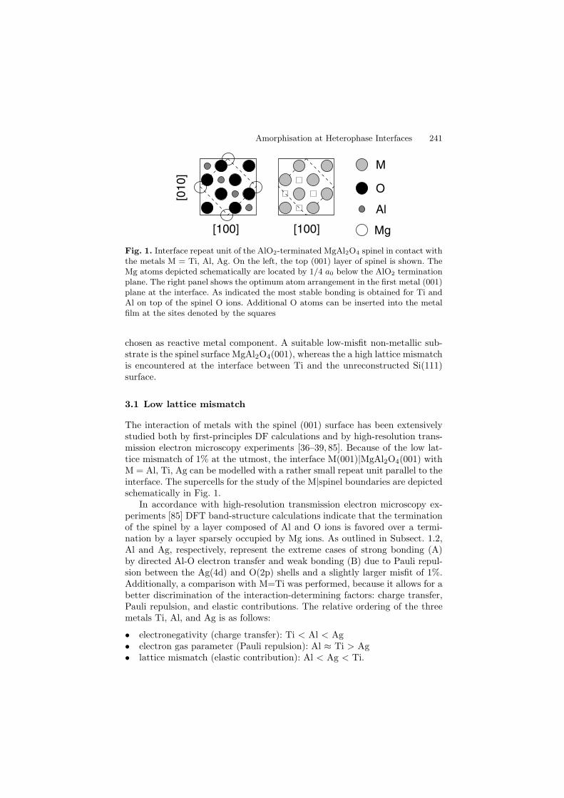
Amorphisation at Heterophase Interfaces 241
[100] [100]
[010]
M
O
Al
Mg
Fig. 1. Interface repeat unit of the AlO2-terminated MgAl2O4 spinel in contact withthe metals M = Ti, Al, Ag. On the left, the top (001) layer of spinel is shown. TheMg atoms depicted schematically are located by 1/4 a0 below the AlO2 terminationplane. The right panel shows the optimum atom arrangement in the first metal (001)plane at the interface. As indicated the most stable bonding is obtained for Ti andAl on top of the spinel O ions. Additional O atoms can be inserted into the metalfilm at the sites denoted by the squares
chosen as reactive metal component. A suitable low-misfit non-metallic sub-strate is the spinel surface MgAl2O4(001), whereas the a high lattice mismatchis encountered at the interface between Ti and the unreconstructed Si(111)surface.
3.1 Low lattice mismatch
The interaction of metals with the spinel (001) surface has been extensivelystudied both by first-principles DF calculations and by high-resolution trans-mission electron microscopy experiments [36–39, 85]. Because of the low lat-tice mismatch of 1% at the utmost, the interface M(001)|MgAl2O4(001) withM = Al, Ti, Ag can be modelled with a rather small repeat unit parallel to theinterface. The supercells for the study of the M|spinel boundaries are depictedschematically in Fig. 1.
In accordance with high-resolution transmission electron microscopy ex-periments [85] DFT band-structure calculations indicate that the terminationof the spinel by a layer composed of Al and O ions is favored over a termi-nation by a layer sparsely occupied by Mg ions. As outlined in Subsect. 1.2,Al and Ag, respectively, represent the extreme cases of strong bonding (A)by directed Al-O electron transfer and weak bonding (B) due to Pauli repul-sion between the Ag(4d) and O(2p) shells and a slightly larger misfit of 1%.Additionally, a comparison with M=Ti was performed, because it allows for abetter discrimination of the interaction-determining factors: charge transfer,Pauli repulsion, and elastic contributions. The relative ordering of the threemetals Ti, Al, and Ag is as follows:
• electronegativity (charge transfer): Ti < Al < Ag• electron gas parameter (Pauli repulsion): Al ≈ Ti > Ag• lattice mismatch (elastic contribution): Al < Ag < Ti.
242 Sibylle Gemming et al.
The electronegativity of an atom is a measure for the binding strength ofits valence electrons. At metal-oxide interfaces, metals with a low electroneg-ativity can act as an electron donor for the undercoordinated oxygen ions ofthe contact plane, which enhances the interfacial bonding. The electron gasparameter is a measure of the local electron density and it is defined as theradius of a sphere which would contain one valence electron if the electrondensity were homogeneous; thus, a low electron gas parameters is characteris-tic of atoms with a high spatial density of electrons, which exhibit the higherpropensity for Pauli repulsion.
The calculated interface distances of d(Al-O) = 1.9 A < d(Ti-O) = 1.99 A
< d(Ag-O) = 2.3 A indicate, that the Ti-containing adhesion system exhibitsan average position between the two pristine boundaries. The work of sepa-ration Wsep was calculated as difference of the total energies of the interfacesystem and the two free component slabs within the same supercell geometry.The values amount toWsep(Al|Sp) = 2.25 J/m2 >Wsep(Ti|Sp) = 1.81 J/m2 >Wsep(Ag|Sp) = 1.10 J/m2 and confirm the intermediate nature of the Ti|spinelboundary. Therefore, the reduction of the Pauli repulsion by the low valenceelectron density of the Ti film is the main driving force for the adhesion en-hancement (titanium effect), whereas the other two contributions balance eachother. A stepwise exchange of Ag atoms by Ti atoms within the first metallayer indicated that the major stabilisation is already reached, when everysecond Ag atom is replaced by Ti.
Thus, the application of Ti as adhesive buffer layer in non-strained systemsis based on its ability to form polar bonds with electronegative partners suchas the O ions in oxide ceramics, but also metallic bonds with electron-richelements such as Ag. This high reactivity has also drawbacks as describedin [41, 42]: The high oxygen affinity of Ti can also induce an autocatalyticuptake of oxygen into a Ti adhesive layer. DFT bandstructure calculationshave shown that the most stable position of the additional O atoms is theinterstitial site indicated by the squares in Fig. 1. In this way, the metallicadhesive Ti layer is transformed into a brittle titanium suboxide, which ex-hibits both a higher Pauli repulsion and a stronger elastic strain contributionthan the free metal. In this manner the reactivity of the interlayer degradesthe long-term stability of the interface in an oxidative environment.
3.2 High lattice mismatch
Many examples for reactive interfaces including amorphous phases are foundat heterophase boundaries between metallic and semiconducting materials,especially at the contacts between a microelectronic device and the bondingmetal. Almost all early transition and rare earth metals bind to the Si(111) orSi(110) surfaces under the formation of binary and ternary silicides. The mostextensively studied material combination is the interface Co|Si, where DFT-based modelling has helped to quantify the thermodynamic driving force forthe formation of silicides like CoSi2 [27–29,86,87]. The first steps of the silicide
Amorphisation at Heterophase Interfaces 243
formation are the migration of Co atoms to interstitial sites in the Si lattice,the diffusion of those atoms along grain boundaries in Si, and the growthof larger CoSi2 crystals from CoSi2 seeds [27]. The interface reconstructionhas also been explained within a DFT framework [28]. Slab calculations ofCoSi2(100)|Si(100) [87], CoSi2(111)|Si(111) [86], and of up to two monolayersof Co on Si(001) [29] confirm that the formation of the reactive oxide doesnot depend on a particular orientation of the substrate. Also the interactionof Y and Gd [30], Sr [31], Ni [88] and Fe [32] with Si has been investigatedtheoretically. A first-principles study of the boundary between Si and an earlytransition metal such as Ti is, however, rendered difficult by the large mis-match of the lattice constants of Ti and Si. With a lattice mismatch of 24%large interface unit cells have to be employed in the interface modelling. Onlywith the application of parallel computing power, such demanding tasks havelately become feasible.
At elevated temperature a deposited layer of Ti reacts with Si(111) orSi(110) surfaces to form several stable silicides at the boundary, which liewithin a composition range of Ti3Si to TiSi2 [89–92]. Depending on depo-sition and preparation conditions, the silicide interlayer is either crystallineor amorphous, and the structural phase transition between those two statesoccurs at a temperature well below the melting point of either of the two con-stituents or of the resultant silicide phase [89, 91, 93–97]. The structural fea-tures, thermodynamic stability, and electronic properties of several bulk TiSixcompounds have also been investigated theoretically [98]. Yet, the quantum-mechanical treatment of the Ti|Si interfaces is difficult, as the lattice para-
meters of hexagonally close-packed Ti (a0 = 2.95 A) and Si in the diamond
structure (a0 = 3.85 A) are quite different. Thus, only every third Si atomroughly coincides with every fourth Ti atom along the close-packed [1-10.0]direction of Ti. An interface model with low remanent elastic stress can beconstructed, which, however, contains a high number of atoms in the supercelland is computationally demanding. Yet, with the emergence of carbon nano-tube integration in Si-based semiconductor devices, the interface between Tiand Si has become an important topic for investigation, because thin Ti inter-layers act as adhesion enhancers both for the nanotube growth catalyst andfor Au contacts to the individual tube [99]. Thus, it is of great technologicalrelevance to study the corresponding interfaces quantitatively, as outlined inthe following section.
4 The Ti(000.1)|Si(111) interface
4.1 Model structures
Due to the considerable lattice mismatch of 26% between the Si(111) andthe Ti(000.1) crystals the appropriate interface supercell spans several latticespacings. For this purpose, the so-called coincidence site lattice is constructed
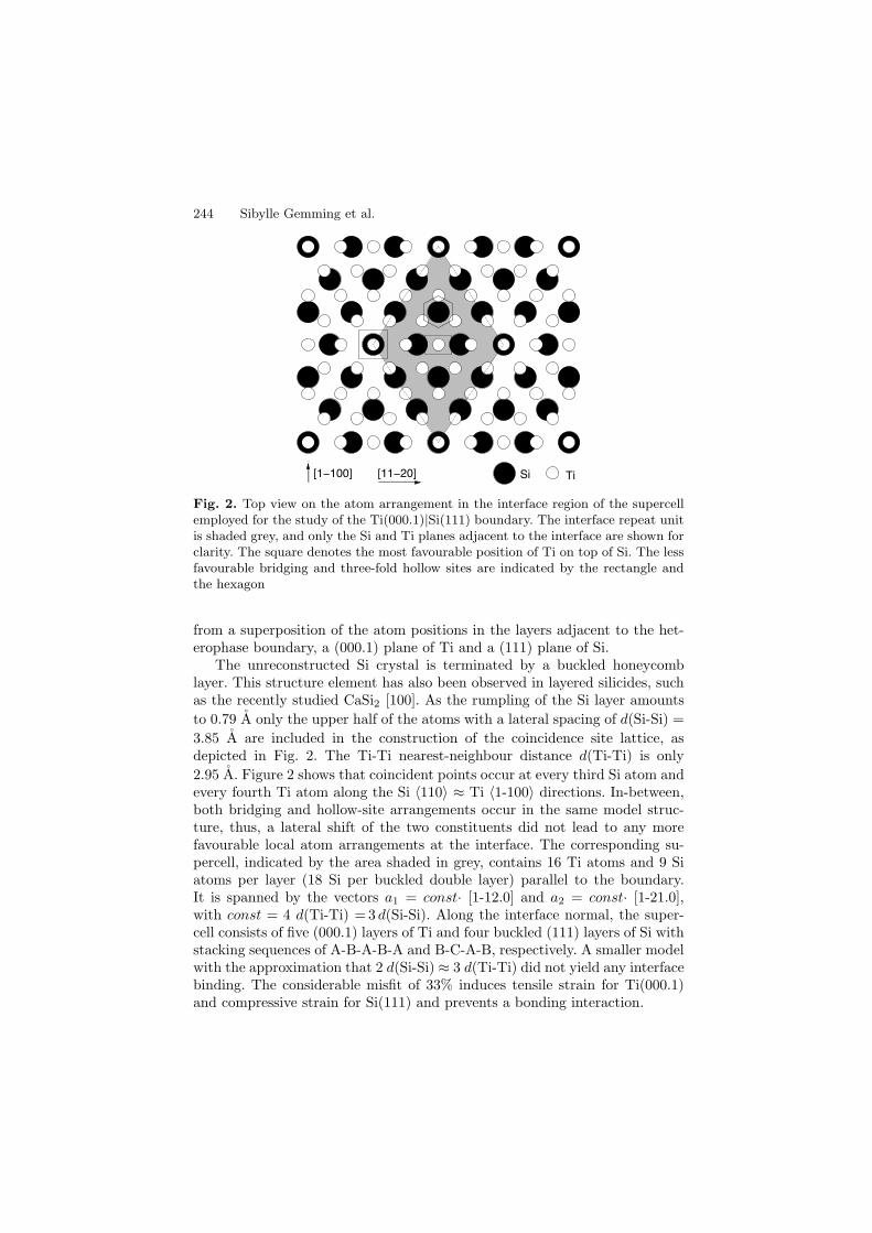
244 Sibylle Gemming et al.
TiSi[1−100] [11−20]
Fig. 2. Top view on the atom arrangement in the interface region of the supercellemployed for the study of the Ti(000.1)|Si(111) boundary. The interface repeat unitis shaded grey, and only the Si and Ti planes adjacent to the interface are shown forclarity. The square denotes the most favourable position of Ti on top of Si. The lessfavourable bridging and three-fold hollow sites are indicated by the rectangle andthe hexagon
from a superposition of the atom positions in the layers adjacent to the het-erophase boundary, a (000.1) plane of Ti and a (111) plane of Si.
The unreconstructed Si crystal is terminated by a buckled honeycomblayer. This structure element has also been observed in layered silicides, suchas the recently studied CaSi2 [100]. As the rumpling of the Si layer amounts
to 0.79 A only the upper half of the atoms with a lateral spacing of d(Si-Si) =
3.85 A are included in the construction of the coincidence site lattice, asdepicted in Fig. 2. The Ti-Ti nearest-neighbour distance d(Ti-Ti) is only
2.95 A. Figure 2 shows that coincident points occur at every third Si atom andevery fourth Ti atom along the Si 〈110〉 ≈ Ti 〈1-100〉 directions. In-between,both bridging and hollow-site arrangements occur in the same model struc-ture, thus, a lateral shift of the two constituents did not lead to any morefavourable local atom arrangements at the interface. The corresponding su-percell, indicated by the area shaded in grey, contains 16 Ti atoms and 9 Siatoms per layer (18 Si per buckled double layer) parallel to the boundary.It is spanned by the vectors a1 = const· [1-12.0] and a2 = const· [1-21.0],with const = 4 d(Ti-Ti) = 3 d(Si-Si). Along the interface normal, the super-cell consists of five (000.1) layers of Ti and four buckled (111) layers of Si withstacking sequences of A-B-A-B-A and B-C-A-B, respectively. A smaller modelwith the approximation that 2 d(Si-Si) ≈ 3 d(Ti-Ti) did not yield any interfacebinding. The considerable misfit of 33% induces tensile strain for Ti(000.1)and compressive strain for Si(111) and prevents a bonding interaction.
Amorphisation at Heterophase Interfaces 245
4.2 Stability at low temperature
Due to the difference between the real lattice mismatch of 26% and the mis-match in the model of only 25% there are remanent elastic deformations,tensile for the Si slab and compressive for the Ti slab. As the bulk elasticproperties of both elements are almost equal, there exists no natural choicewhether the lengths of the in-plane vectors |a1| = |a2| spanning the supercell
ought to amount to 3 d(Si-Si) = 11.55 A or to 4 d(Ti-Ti) = 11.8 A. Thus, thestructure optimisation of the interface was carried out for both cases and alsofor the arithmetic mean. Within this range of values the total energy of thesystem does not significantly depend on the choice of a1 and a2. This effectis presumably related to the similarity of the bulk moduli (both about 110GPa), which means that in this range of values the lattice expansion of Si andthe lattice compression of Ti lead to a comparable energy change. Thus, theresults obtained for |a1| = |a2| = 3 d(Si-Si) will be discussed in the following,because this choice reflects best the experimental setup, where a Ti contactlayer is evaporated onto a comparatively massive Si substrate.
Structure optimisation yields a supercell height of c = 24.06 A, whichcorresponds to an interface contraction of 0.16 A. On the Si side the bucklingof the double layer next to the interface is strongly diminished by 0.21 A,whereas the spacing to the next lower double layer is reduced by only 0.06 A.This indicates that all Si atoms of the buckled layer interact with the Ti atoms.On the Ti side, the last layer is slightly curved by 0.09 A, and the averagedistance between this Ti layer and the next one is reduced by 0.06 A. TheTi-Si distances vary from 2.55 A at the on-top position to 2.71 A at the hollowsites. There, an additional Si atom from the lower part of the Si double layerrelaxes towards the interface such that the Ti-Si distance amounts to 2.76 A,and the effective coordination number of Ti with respect to Si partners isenhanced to four.
The work of separationWsep with respect to the free Si(111) and Ti(000.1)slabs is calculated as the difference of the total energies of the interface,Etot(Ti(000.1)|Si(111)), and the free slabs, Etot(Ti(000.1)) and Etot(Si(111)).The obtained low value of Wsep = 0.27 J/m2 reflects the only weakly attrac-tive interaction at the unreacted interface. The low work of separation is, ofcourse, related to the low density of only 11% of favourable, on-top interactionsites at the boundary. When normalised to this low density of binding sites,an upper bound for the separation energy is obtained, which is of the order of2 J/m2. This value compares well with the work of separation calculated forthe strain-free M|spinel systems. This argument is corroborated by an analy-sis of the binding electron density, obtained as difference between the electrondensity of the total interface and the densities of the free, unrelaxed slabs.An electron transfer from Ti to Si takes place, which is limited to the first Silayer and exhibits the highest accumulation at the Si atom bonded on top ofa Ti atom. Within the Ti slab the density difference decays rapidly as a resultof the very effective metallic screening. In the Si slab, further, but smaller
246 Sibylle Gemming et al.
electron density oscillations can be monitored also in the second layer belowthe interface. This observation reflects the expectation that the screening ofa charge accumulation is less effective in semiconductors. At the interface,some electron density accumulation occurs also at the bridge and three-foldhollow-site positions. Thus, of all adhesion sites only the ones with the short-est Ti-Si distances along the [1-10.0] direction contribute to the binding, whilefor the other sites no favourable interaction is detected. These observationsalso rationalise the low, rather anisotropic binding energy.
4.3 High-temperature behaviour
Experimental investigations indicate the formation of the modifications Ti5Si3,TiSi, and TiSi2 at elevated temperatures, therefore full DFT molecular-dynamics calculations were carried out for the Ti(000.1)|Si(111) interface,employing the supercell described above. In order to study the amorphisationprocess at the interface, the optimised, unreacted structure was employed asstarting geometry. The temperature was raised in one step and controlled bya velocity rescaling algorithm at constant volume. These simulation condi-tions resemble best the setup of the laser heating experiments, which yieldeddetailed experimental data on the phase transformations at the Ti|Si inter-face [95].
For T = 300 K initially the stress tensor σ is anisotropic, with compo-nents σ|| = 13 GPa parallel and σ⊥ = 8 GPa normal to the interface. Evenafter several picoseconds of relaxation time the two stress tensor componentsdo not equilibrate. Therefore, the simulation was also performed at an ele-vated temperature of T = 600 K, at which the formation of films with thestoichiometry TiSi has been reported [89]. For this temperature, the initialstress tensor components exhibit a higher value of about 23 GPa due to theboundary condition which is given by the lateral lattice periodicity of Si assubstrate material. However, the internal stresses are equilibrated and loweredto 20 GPa after a relaxation time of only 1 ps. The stress reduction is accom-panied by the reorientation of atoms in the boundary region. At the highertemperature the increased kinetic energy of the atoms induces a rougheningof the interface, which now comprises the Ti(000.1) layer and the full Si(111)double layer adjacent to the interface. In this way, a non-crystalline film isobtained at the boundary. The area density of atoms within this boundaryfilm yields indeed a stoichiometry of about Ti : Si = 1 : 1.
Since the supercell is repeated periodically, the model film obtained here isonly an approximant of the structure of the real, amorphous boundary phase.However, one can evaluate the short-range part of the radial distribution func-tion within the limits set by the minimum image convention, i.e. one half ofthe supercell dimensions. For the cell employed here this amounts to about5 A, thus the first coordination sphere can safely be analysed. In order tocover only the bond lengths at the interface, the bond lengths were calculatedin real space and weigthed according to their frequency of occurence. For the
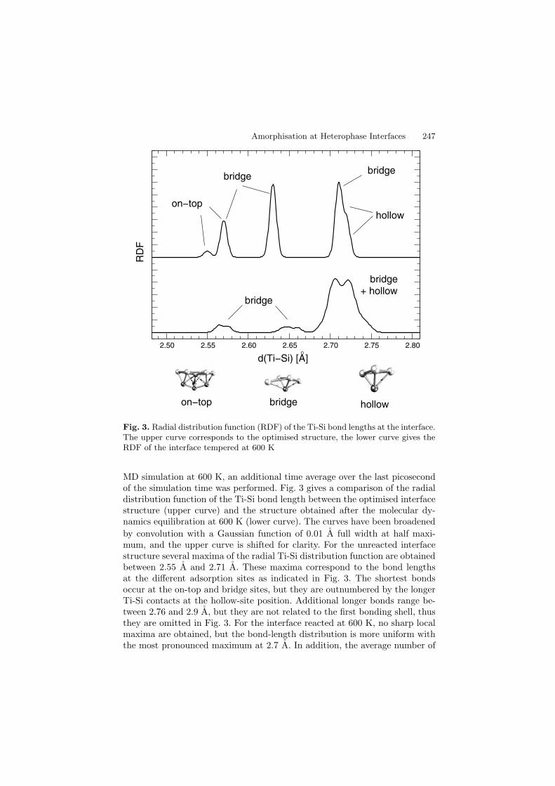
Amorphisation at Heterophase Interfaces 247
2.5 2.55 2.6 2.65 2.7 2.75 2.8
0
2
4
6
8
10
12
14
16
18
20
22
24
26
28
hollowbridgeon−top
bridge
bridge+ hollow
bridgebridge
on−tophollow
2.802.752.702.652.602.552.50
RD
F
d(Ti−Si) [A]
Fig. 3. Radial distribution function (RDF) of the Ti-Si bond lengths at the interface.The upper curve corresponds to the optimised structure, the lower curve gives theRDF of the interface tempered at 600 K
MD simulation at 600 K, an additional time average over the last picosecondof the simulation time was performed. Fig. 3 gives a comparison of the radialdistribution function of the Ti-Si bond length between the optimised interfacestructure (upper curve) and the structure obtained after the molecular dy-namics equilibration at 600 K (lower curve). The curves have been broadened
by convolution with a Gaussian function of 0.01 A full width at half maxi-mum, and the upper curve is shifted for clarity. For the unreacted interfacestructure several maxima of the radial Ti-Si distribution function are obtainedbetween 2.55 A and 2.71 A. These maxima correspond to the bond lengthsat the different adsorption sites as indicated in Fig. 3. The shortest bondsoccur at the on-top and bridge sites, but they are outnumbered by the longerTi-Si contacts at the hollow-site position. Additional longer bonds range be-tween 2.76 and 2.9 A, but they are not related to the first bonding shell, thusthey are omitted in Fig. 3. For the interface reacted at 600 K, no sharp localmaxima are obtained, but the bond-length distribution is more uniform withthe most pronounced maximum at 2.7 A. In addition, the average number of
248 Sibylle Gemming et al.
bonds is by 10% lower than the corresponding number of bonds at the opti-mised interface. These findings reflect the equilibration of the bond lengthsand the local coordination spheres upon reaction at the interface.
Concomitant with the geometry change, the total energy of the super-cell relaxed at 600 K is lower than the total energy of the starting structureobtained from the geometry optimisation (formally at 0 K). This leads to adoubling of the work of separation to 0.52 J/m2. Thus, the release of theelastic energy, which is stored in the atomically flat structure model yields asignificant stabilisation of the boundary. The results also confirm experimen-tal findings that TiSi occurs as an intermediate reaction product towards thefinal high-temperature phase, TiSi2. Since the further reaction to a full TiSi2layer at the boundary would require the use of even larger supercells, fur-ther investigations are currently carried out on two separate model systems,Si(111)|TiSi2(000.1) and Ti(000.1)|TiSi2(000.1). Preliminary results from thestructure optimisation indicate that the values of the work of separation willexceed 1 J/m2. Thus, a further stabilisation of the interface by the formationof the disilicide is predicted.
5 Conclusions
The detailed description of the stability of and the structure formation atreactive interfaces requires an electronic-structure based method, which canproperly account for local electron redistributions and subtle changes of thecoordination number. Band-structure calculations based on the DFT providethe suitable theoretical framework for the investigations of such systems, andthe application of parallel computing supplies the required numerical power.The most efficient way to exploit this power is provided by parallelisationover an optimised set of integration points, which split the solution of theKohn-Sham equations into a set of matrix equations with equal matrix sizes.With this approach two reactive systems, both employing the element Ti asmetallic component, have been studied to elucidate and quantify the role,which electronic and elastic contributions play in interface reactivity.
For an interface with low lattice misfit such as M|MgAl2O4(001) (M = Ti,Al, Ag) the balance of electronic factors dominates the structure and stability.If the electronegativity difference between metal and substrate favours electrontransfer, a directed bonding of the metal on top of the O ions is obtained. Thissituation occurs for M = Ti and Al. Otherwise, the Pauli repulsion betweenthe Ag(4d) shell and the O(2p) shell leads to a weaker adhesion on the hollowsites of the spinel surface. Furthermore, the reactive metal Ti can undergoan autocatalytic oxygen uptake at the octahedral interstitial site, which thenleads to an oxidative corrosion of Ti interlayers.
Ti(000.1)|Si(111) is a system with a high lattice mismatch and a rich in-terface chemistry. The ternary interface phase ranges from Ti-rich Ti5Si3 to
Amorphisation at Heterophase Interfaces 249
Si-rich TiSi2, which is the thermodynamically most stable phase. DFT in-vestigations show, that the electron transfer at the unreacted interface leadsto a weakly bonding interaction, because only a small number of favourablebonding sites can be saturated. DFT molecular-dynamics simulations at an el-evated temperature of 600 K facilitate the release of elastic stresses still storedin the unreacted interface. The concomitant interface roughening leads to anequilibration of the Ti-Si bond lengths and a doubling of the interface stability.Thus, at this boundary, electron transfer processes and elastic contributionsinfluence the binding energy equally strongly.
The comparison of the two model cases in which the same metal exhibitsquite different reactivity shows that a realistic material modelling has to ac-count for both electron transfer across the interface and elastic factors parallelto the interface equally well. Simplified approaches, neglecting the details ofthe electronic structure, may predict the properties of non-reactive boundaries.However, the fine balance between influence factors at reactive boundaries in-deed requires the more accurate treatment provided by the density-functionalfirst-principles modelling.
References
1. R.C. Longo, V.S. Stepanyuk, W. Hegert, A. Vega, L.J. Gallego, J. Kirschner.Interface intermixing in metal heteroepitaxy on the atomic scale. Phys. Rev. B,69:073406, 2004.
2. J.E. Houston, J.M. White, P.J. Feibelman, D.R. Hamann. Interface-state prop-erties for strained-layer Ni adsorbed on Ru(0001). Phys. Rev. B, 38:12164, 1988.
3. R.E. Watson, M. Weinert, J.W. Davenport. Structural stabilities of layeredmaterials: Pt–Ta. Phys. Rev. B, 35:9284, 1987.
4. H.R. Gong, B.X. Liu. Interface stability and solid-state amorphization in animmiscible Cu–Ta system. Appl. Phys. Lett., 83:4515, 2003.
5. S. Narasimham. Stress, strain, and charge transfer in Ag/Pt(111): A test ofcontinuum elasticity theory. Phys. Rev. B, 69:045425, 2004.
6. S. Gemming, M. Schreiber. Nanoalloying in mixed AgmAun nanowires.Z. Metallkd., 94:238, 2003.
7. S. Gemming, G. Seifert, M. Schreiber. Density functional investigation of gold-coated metallic nanowires. Phys. Rev. B, 69:245410, 2004.
8. S. Gemming, M. Schreiber. Density-functional investigation of alloyed metallicnanowires. Comp. Phys. Commun., 169:57, 2005.
9. P.J. Lin-Chung, T.L. Reinecke. Antisite defect in GaAs and at the GaAs–AlAsinterface. J. Vac. Sci. Technol., 19:443, 1981.
10. S. Das Sarma, A. Madhukar. Ideal vacancy induced band gap levels in latticematched thin superlattices: The GaAs–AlAs(100) and GaSb–InAs(100) sys-tems. J. Vac. Sci. Technol., 19:447, 1981.
11. Y. Wei, M. Razeghi. Modeling of type-II InAs/GaSb superlattices using an em-pirical tight-binding method and interface engineering. Phys. Rev. B, 69:085316,2004.
12. A. Kley, J. Neugebauer. Atomic and electronic structure of the GaAs/ZnSe(001)interface. Phys. Rev. B, 50:8616, 1994.
250 Sibylle Gemming et al.
13. W.R.L. Lambrecht, B. Segall. Electronic structure and bonding at SiC/AlNand SiC/BP interfaces. Phys. Rev. B, 43:7070, 1991.
14. L. Pizzagalli, G. Cicero, A. Catellani. Theoretical investigations of a highlymismatched interface: SiC/Si(001). Phys. Rev. B, 68:195302, 2003.
15. P. Casek, S. Bouette-Russo, F. Finocchi, C. Noguera. SrTiO3(001) thin filmson MgO(001): A theoretical study. Phys. Rev. B, 69:085411, 2004.
16. R.R. Das, Y.I. Yuzyuk, P. Bhattacharya, V. Gupta, R.S. Katiyar. Foldedacoustic phonons and soft mode dynamics in BaTiO3/SrTiO3 superlattices.Phys. Rev. B, 69:132301, 2004.
17. S. Hutt, S. Kostlmeier, C. Elsasser. Density functional study of the Σ3/(111)grain boundary in strontium titanate. J. Phys.: Condens. Matter, 13:3949, 2001.
18. S. Gemming, M. Schreiber. Impurity and vacancy clustering at theΣ3(111)[1-10] grain boundary in strontium titanate. Chem. Phys., 309:3, 2005.
19. M. Sternberg, W.R.L. Lambrecht, T. Frauenheim. Molecular-dynamics studyof diamond/silicon (001) interfaces with and without graphitic interface layers.Phys. Rev. B, 56:1568, 1997.
20. T. Sakurai, T. Sugano. Theory of continuously distributed trap states atSi–SiO2 interfaces. J. Appl. Phys., 52:2889, 1981.
21. D. Chen, X.L. Ma, Y.M. Wang, L. Chen. Electronic properties and bondingconfiguration at theTiN/MgO(001) interface. Phys. Rev. B, 69:155401, 2004.
22. R. Puthenkovilakam, E.A. Carter, J.P. Chang. First-principles exploration ofalternative gate dielectrics: Electronic structure of ZrO2/Si and ZrSiO4/Si in-terfaces. Phys. Rev. B, 69:155329, 2004.
23. M. Ruhle, A.G. Evans. High toughness ceramics and ceramic composites. Progr.Mat. Sci., 33:85, 1989.
24. G. Willmann, N. Schikora, R.P. Pitto. Retrieval of ceramic wear couples in totalhip arthroplasty. Bioceram., 15:813, 1994.
25. A.M. Freborg, B.L. Ferguson, W.J. Brindley, G.J. Petrus. Modeling oxidationinduced stresses in thermal barrier coatings. Mater. Sci. Eng. A, 245:182, 1998.
26. R. Benedek, M. Minkoff, L.H. Yang. Adhesive energy and charge transfer forMgO/Cu heterophase interfaces. Phys. Rev. B, 54:7697, 1996.
27. A. Horsfield, H. Fujitani. Density-functional study of the initial stage of theanneal of a thin Co film on Si. Phys. Rev. B, 63:235303, 2001.
28. B.D. Yu, Y. Miyamoto, O. Sugino, A. Sakai, T. Sasaki, T. Ohno. Structuraland electronic properties of metal-silicide/silicon interfaces: A first-principlesstudy. J. Vac. Sci. Technol. B, 19:1180, 2001.
29. B.S. Kang, S.K. Oh, H.J. Kang, K.S. Sohn. Energetics of ultrathin CoSi2 filmon a Si(001) surface. J. Phys.: Condens. Matter, 15:67, 2003.
30. C. Rogero, C. Koitzsch, M.E. Gonzalez, P. Aebi, J. Cerda, J.A. Martin-Glago.Electronic structure and Fermi surface of two-dimensional rare-earth silicidesepitaxially grown on Si(111). Phys. Rev. B, 69:045312, 2004.
31. C.R. Ashman, C.J. Forst, K. Schwarz, P.E. Blochl. First-principles calculationsof strontium on Si(001). Phys. Rev. B, 69:075309, 2004.
32. S. Walter, F. Blobner, M. Krause, S. Muller, K. Heinz, U. Starke. Interfacestructure and stabilization of metastable B2-FeSi/Si(111) studied with low-energy electron diffraction and density functional theory. J. Phys.: Condens.Matter, 15:5207, 2003.
33. U. Schoenberger, O.K. Andersen, M. Methfessel. Bonding at metal ceramicinterfaces – Ab-initio density-functional calculations for Ti and Ag on MgO.Acta Metall. Mater., 40:S1, 1992.
Amorphisation at Heterophase Interfaces 251
34. K. Kruse, M.W. Finnis, J.S. Lin, M.C. Payne, V.Y. Milman, A. DeVita, M.J.Gillan. First-principles study of the atomistic and electronic structure of theniobium–α-alumina(0001) interface. Phil. Mag. Lett., 73:377, 1996.
35. Y. Ikuhara, Y. Sugawara, I. Tanaka, P. Pirouz. Atomic and electronic structureof V/MgO interface. Interface Science, 5:5, 1997.
36. R. Schweinfest, S. Kostlmeier, F. Ernst, C. Elsasser, T. Wagner, M.W. Finnis.Atomistic and electronic structure of Al/MgAl2O4 and Ag/MgAl2O4 interfaces.Phil. Mag. A, 81:927, 2000.
37. S. Kostlmeier, C. Elsasser. Ab-initio investigation of metal-ceramic bonding.M(001)/MgAl2O4, M=Al, Ag. Interface Science, 8:41, 2000.
38. S. Kostlmeier, C. Elsasser, B. Meyer, M.W. Finnis. Ab initio study of electronicand geometric structures of metal/ceramic heterophase boundaries. Mat. Res.Soc. Symp. Proc., 492:97, 1998.
39. S. Kostlmeier, C. Elsasser, B. Meyer, M.W. Finnis. A density-functional studyof interactions at the metal-ceramic interfaces Al/MgAl2O4 and Ag/MgAl2O4.phys. stat. sol. (a), 166:417, 1998.
40. S. Kostlmeier, C. Elsasser. Density functional study of the “titanium effect” atmetal/ceramic interfaces. J. Phys.: Condens. Matter, 12:1209, 2000.
41. C. Elsasser, S. Kostlmeier-Gemming. Oxidative corrosion of adhesive interlay-ers. Phys. Chem. Chem. Phys., 3:5140, 2001.
42. S. Kostlmeier, C. Elsasser. Oxidative corrosion of adhesive interlayers. Mat.Res. Soc. Symp. Proc., 586:M3.1, 1999.
43. V. Vitek, G. Gutekunst, J. Mayer, M. Ruhle. Atomic structure of misfit dislo-cations in metal-ceramic interfaces. Phil. Mag. A, 71:1219, 1996.
44. J.-H. Cho, K.S. Kim, C.T. Chan, Z. Zhang. Oscillatory energetics of flat Agfilms on MgO(001). Phys. Rev. B, 63:113408, 2001.
45. C. Klein, G. Kresse, S. Surnev, F.P. Netzer, M. Schmidt, P. Varga. Vanadiumsurface oxides on Pd(111): A structural analysis. Phys. Rev. B, 68:235416, 2003.
46. A. Trampert, F. Ernst, C.P. Flynn, H.F. Fischmeister and M. Ruhle. High-resolution transmission electron microscopy studies of the Ag/MgO interface.Acta Metall. Mater., 40:S227, 1992.
47. A.M. Stoneham, P.W. Tasker. Metal non-metal and other interfaces – The roleof image interactions. J. Phys. C, 18:L543, 1985.
48. D.M. Duffy, J.H. Harding, A.M. Stoneham. Atomistic modeling of the metal-oxide interface with image interactions. Acta Metall. Mater., 40:S11, 1992.
49. D.M. Duffy, J.H. Harding, A.M. Stoneham. Atomistic modeling of metal-oxideinterfaces with image interactions. Phil. Mag. A, 67:865, 1993.
50. M.W. Finnis. Metal ceramic cohesion and the image interaction. Acta Metall.Mater., 40:S25, 1992.
51. A.M. Stoneham, P.W. Tasker. Image charges and their influence on the growthand the nature of thin oxide-films. Phil. Mag. B, 55:237, 1987.
52. D.A. Muller, D.A. Shashkov, R. Benedek, L.H. Yang, J. Silcox, D.N. Seidman.Adhesive energy and charge transfer for MgO/Cu heterophase interfaces. Phys.Rev. Lett., 80:4741, 1998.
53. T. Ochs, S. Kostlmeier, C. Elsasser. Microscopic structure and bonding at thePd/SrTiO3(001) interface. Integr. Ferroelectr., 30:251, 2001.
54. A. Zaoui. Energetic stabilities and the bonding mechanism ofZnO(0001)/Pd(111) interfaces. Phys. Rev. B, 69:115403, 2004.
252 Sibylle Gemming et al.
55. M. Christensen, S. Dudiy, G. Wahnstrom. First-principles simulation of metal-ceramic interface adhesion: Cu/WC versus Cu/TiC. Phys. Rev. B, 65:045408,2002.
56. M. Christensen, G. Wahnstrom. Co-phase penetration of WC(10-10)/WC(10-10) grain boundaries from first principles. Phys. Rev. B, 67:115415,2003.
57. J. Hartford. Interface energy and electron structure for Fe/VN. Phys. Rev. B,61:2221, 2000.
58. E. Saiz, A.P. Tomsia, R.M. Cannon. Ridging effects on wetting and spreadingof liquids on solids. Acta Mater., 46:2349, 1998.
59. J.A. Venables, G.D.T. Spiller, M. Hanbucken. Nucleation and growth of thinfilms. Rep. Prog. Phys., 47:399, 1984.
60. A.M. Stoneham, J.H. Harding. Not too big, not too small: The appropriatescale. Nature Materials, 2:65, 2003.
61. M.W. Finnis. Interatomic Forces in Condensed Matter. Oxford UniversityPress, Oxford, 2003.
62. R.O. Jones, O. Gunnarsson. Density-functional theory. Rev. Mod. Phys., 61:689,1989.
63. H. Eschrig. The Fundamentals of Density Functional Theory. Edition amGutenbergplatz, Leipzig, 2003.
64. G. Onida, L. Reining, A. Rubio. Electronic excitations: density-functional ver-sus many-body Green’s-function approaches. Rev. Mod. Phys., 74:601, 2002.
65. R.M. Dreizsler, E.K.U. Gross. Density Functional Theory. Springer, Berlin,1990.
66. R.G. Parr, W. Yang. Density-Functional Theory of Atoms and Molecules. Ox-ford University Press, New York, 1989.
67. P. Hohenberg, W. Kohn. Inhomogeneous electron gas. Phys. Rev., 136:B864,1964.
68. M. Levy. Electron densities in search of Hamiltonians. Phys. Rev. A, 26:1200,1982.
69. U. von Barth, L. Hedin. The energy density functional formalism for excitedstates. J. Phys. C, 5:1629, 1972.
70. N.D. Mermin. Thermal properties of the inhomogeneous electron gas. Phys.Rev., 137:A1441, 1965.
71. S.H. Vosko, L. Wilk, M. Nusair. Accurate spin-dependent electron liquid cor-relation energies for local spin density calculations: a critical analysis. Can. J.Phys., 58:1200, 1980.
72. O. Gunnarsson, M. Jonson, B.I. Lundqvist. Descriptions of exchange and corre-lation effects in inhomogeneous electron systems. Phys. Rev. B, 20:3136, 1979.
73. J.-M. Jancu, R. Scholz, F. Beltram, F. Bassani. Empirical spds* tight-bindingcalculation for cubic semiconductors: General method and material parameters.Phys. Rev. B, 57:6493, 1998.
74. R. Scholz, J.-M. Jancu, F. Bassani. Superlattice calculation in an empiricalspds* tight-binding model. Mat. Res. Soc. Symp. Proc., 491:383, 1998.
75. A. Di Carlo. Time-dependent density-functional-based tight-binding. Mat. Res.Soc. Symp. Proc., 491:391, 1998.
76. C.Z. Wang, K.M. Ho, C.T. Chan. Tight-binding molecular-dynamics study ofamorphous carbon. Phys. Rev. Lett., 70:611, 1993.
Amorphisation at Heterophase Interfaces 253
77. P. Ordejon, D. Lebedenko, M. Menon. Improved nonorthogonal tight-bindingHamiltonian for molecular-dynamics simulations of silicon clusters. Phys. Rev.B, 50:5645, 1994.
78. M. Menon, K.R. Subbaswamy. Nonorthogonal tight-binding molecular-dynamics scheme for silicon with improved transferability. Phys. Rev. B,55:9231, 1997.
79. C.M. Goringe, D.R. Bowler, E. Hernandez. Tight-binding modelling of materi-als. Rep. Prog. Phys., 60:1447, 1997.
80. A. Di Carlo, M. Gheorghe, P. Lugli, M. Sternberg, G. Seifert, T. Frauenheim.Theoretical tools for transport in molecular nanostructures. Physica B, 314:86,2002.
81. R. Car, M. Parrinello. Unified approach for molecular dynamics and density-functional theory. Phys. Rev. Lett., 55:2471, 1985.
82. D. R. Hamann, M. Schluter, C. Chiang. Norm-conserving pseudopotentials.Phys. Rev. Lett., 43:1494, 1979.
83. G.B. Bachelet, D.R. Hamann, M. Schluter. Pseudopotentials that work: FromH to Pu. Phys. Rev. B, 26:4199, 1082.
84. J. Moreno, J.M. Soler. Optimal meshes fur integrals in real- and reciprocal-spaceunit cells. Phys. Rev. B, 45:13891, 1992.
85. R. Schweinfest, Th. Wagner, F. Ernst. Annual Report to the VW Foundationon the Project Progress. Stuttgart, 1997.
86. R. Stadler, D. Vogtenhuber, R. Podloucky. Ab initio study of theCoSi2(111)/Si(111) interface. Phys. Rev. B, 60:17112, 1999.
87. R. Stadler, R. Podloucky. Ab initio studies of the CuSi2(100)/Si(100) interface.Phys. Rev. B, 62:2209, 2000.
88. H. Fujitani. First-principles study of the stability of the NiSi2/Si(111) interface.Phys. Rev. B, 57:8801, 1998.
89. B. Chenevier, O. Chaix-Pluchery, P. Gergaud, O. Thomas, F. La Via. Thermalexpansion and stress development in the first stages of silicidation in Ti/Si thinfilms. J. Appl. Phys., 94:7083, 2003.
90. G. Kuri, Th. Schmidt, V. Hagen, G. Materlik, R. Wiesendanger, J. Falta. Sub-surface interstitials as promoters of three-dimensional growth of Ti on Si(111):An x-ray standing wave, x-ray photoelectron spectroscopy, and atomic forcemicroscopy investigation. J. Vac. Sci. Technol. A, 20:1997, 2002.
91. J.M. Yang, J.C. Park, D.G. Park, K.Y. Lim, S.Y. Lee, S.W. Park, Y.J. Kim. Epi-taxial C49-TiSi2 phase formation on the silicon (100). J. Appl. Phys., 94:4198,2003.
92. O.A. Fouad, M. Yamazato, H. Ichinose, M. Nagano. Titanium disilicide for-mation by rf plasma enhanced chemical vapor deposition and film properties.Appl. Surf. Sci., 206:159, 2003.
93. R. Larciprete, M. Danailov, A. Barinov, L. Gregoratti, M. Kiskinova. Thermaland pulsed laser induced surface reactions in Ti/Si(001) interfaces studied byspectromicroscopy with synchrotron radiation. J. Appl. Phys., 90:4361, 2001.
94. M.S. Alessandrino, M.G. Grimaldi, F. La Via. C49-C54 phase transition inanometric titanium disilicide nanograins. Microelec. Eng., 64:189, 2003.
95. L. Lu, M.O. Lai. Laser induced transformation of TiSi2. J. Appl. Phys., 94:4291,2003.
96. S.L. Cheng, H.M. Lo, L.W. Cheng, S.M. Chang, L.J. Chen. Effects of stresson the interfacial reactions of metal thin films on (001)Si. Thin Solid Films,424:33, 2003.
254 Sibylle Gemming et al.
97. C.C. Tan, L. Lu, A. See, L. Chan. Effect of degree of amorphization of Si onthe formation of titanium silicide. J. Appl. Phys., 91:2842, 2002.
98. M. Ekman, V. Ozolins. Electronic structure and bonding properties of titaniumsilicides. Phys. Rev. B, 57:4419, 1998.
99. F. Wakaya, Y. Ogi, M. Yoshida, S. Kimura, M. Takai, Y. Akasaka, K. Gamo.Cross-sectional transmission electron microscopy study of the influence of nio-bium on the formation of titanium silicide in small-feature contacts. Micr. Eng.,73:559, 2004.
100. S. Gemming, G. Seifert. Nanotube bundles from calcium disilicide - a DFTstudy. Phys. Rev. B, 68:075416-1–7, 2003.
Energy-Level and Wave-Function Statisticsin the Anderson Model of Localization
Bernhard Mehlig1 and Michael Schreiber2
1 Gothenburg University, Department of Physics41296 Goteborg, [email protected]
2 Technische Universitat Chemnitz, Institut fur Physik09107 Chemnitz, [email protected]
1 Introduction
Universal aspects of correlations in the spectra and wave functions of closed,complex quantum systems can be described by random-matrix theory (RMT)[1]. On small energy scales, for example, the eigenvalues, eigenfunctions andmatrix elements of disordered quantum systems in the metallic regime [2] orthose of classically chaotic quantum systems [3] exhibit universal statisticalproperties very well described by RMT. It is now also well established thatdeviations from RMT behaviour are often significant at larger energy scales.
In the case of classically chaotic quantum systems, this was first discussedby Berry using a semiclassical approach and the so-called diagonal approx-imation (for a review see [3]). In the case of classically diffusive, disorderedquantum systems, non-universal deviations from universal spectral fluctua-tions (as described by RMT) were first discussed in [4], using diagrammaticperturbation theory.
Andreev and Altshuler [5] have used an approach based on the non-linearsigma model to calculate non-universal deviations in the spectral statisticsof disordered quantum systems from RMT behaviour, on all energy scales.On energy scales much larger than the mean level spacing, the results of di-agrammatic perturbation theory are reproduced in this way, and thus thenon-universal deviations (from the RMT predictions) derived in [4]. As hasbeen shown in [6], diagrammatic perturbation theory and semiclassical argu-ments combined with the diagonal approximation are essentially equivalent inthis regime.
In [5] it was also argued that non-universal corrections affect the spectraltwo-point correlation function not only on large energy scales, but also onsmall energy scales, of the order of the mean level spacing. This may appearsurprising, but it was explained in [7] that this is just a consequence of the
256 Bernhard Mehlig and Michael Schreiber
fact that the two-point correlation function is well approximated by a sum ofshifted Gaussians.
Turning to eigenfunction statistics, deviations from RMT behaviour inclassically chaotic quantum systems due to so-called scars (that are wavefunctions localized in the vicinity of unstable classical periodic orbits [8]) wereanalyzed in [9]. In disordered quantum systems, deviations from universalwave-function statistics from RMT behaviour, due to increased localisation,have been studied using the non-linear sigma model. For a summary of resultssee [10, 11]. The deviations are most significant in the tails of distributionfunctions [12], of wave-function amplitudes [13–18], of the local density ofstates [13,18], of inverse participation ratios [18], and of NMR line shapes [13].
In the following, exact-diagonalization results for the so-called Andersonmodel of localization are reviewed. The exact diagonalizations were made pos-sible by employing the Lanczos algorithm described in [19]. We concentrate ondeviations from RMT in spectral and wave-function statistics in the quasi-one-dimensional case. The remainder of this brief review is organized as follows.In Sect. 2 the Hamiltonian is written down, and the quantities computed aredefined: the distribution of wave-function intensities and the spectral formfactor. Theoretical expectations are briefly summarized in Sect. 3. The mate-rial in this section is largely taken from [11] and, to some extent, also from [7].In Sect. 4 the exact-diagonalisation results are described. The numerical re-sults on wave-function statistics described in this brief review were publishedin [9, 20, 21]. The analytical and numerical results on spectral statistics wereobtained in collaboration with M. Wilkinson [7,22]. The problem of analyzingstatistical properties of quantum-mechanical matrix elements is not addressedin this brief review. Results based on exact diagonalisation and semiclassicalmethods can be found in [23–25].
2 Formulation of the problem
2.1 The Hamiltonian
The Anderson model [26] is defined by the tight-binding Hamiltonian on ad-dimensional hypercubic lattice
H =∑
r,r′
trr′c†r cr′ +
∑
r
υrc†rcr . (1)
Here c†r and cr are the creation and annihilation operators of an electron onsite r, the hopping amplitudes are usually chosen as trr′ = 1 for nearest-neighbour sites and zero otherwise. Below we summarise the results of exactdiagonalizations for lattices with 64× 4× 4, 128× 4× 4 and 128× 8× 8 sites,using open boundary conditions in the longitudinal direction and periodicboundary conditions in the transversal directions. The on-site potentials υr
are Gaussian distributed with zero mean and
Energy-Level and Wave-Function Statistics 257
〈υrυr′〉 =W 2
12δrr′ . (2)
As usual, the parameterW characterises the strength of the disorder and 〈· · · 〉denotes the disorder average.
As is well-known, the eigenvalues Ej and eigenfunctions ψj of this Hamil-tonian, in the metallic regime, exhibit fluctuations described by RMT. De-pending on the symmetry, Dyson’s Gaussian orthogonal or unitary ensem-bles [27] are appropriate. The former applies in the absence of magnetic fieldsor more generally when the secular matrix is real symmetric. With magneticfield, complex phases for the hopping matrix elements yield a unitary secularmatrix. We refer to these cases by assigning, as usual, the parameter β = 1to the former and β = 2 to the latter. The metallic regime is characterizedby g ≫ 1 where g = 2πν0DL
d−2 is the dimensionless conductance. Hereν0 = 1/(V ∆) is the average density of states per unit volume, ∆ is the meanlevel spacing (that is the average spacing between neighbouring energy levels),and V = Ld is the volume. D = vFτℓ/d is the (dimensionless) diffusion con-stant, determined by the collision time τℓ = ℓ/vF (here ℓ is the mean free path,that is the average distance travelled between two subsequent collisions withthe impurity potential), and the Fermi velocity vF. Four length scales are im-portant: the lattice spacing a, the linear dimension L, the localization lengthξ, and the mean free path ℓ. In the following the diffusive limit is considered,where ℓ≪ L. We also require that L, ξ, ℓ≫ a.
2.2 Wave-function statistics
By diagonalizing the Hamiltonian H using the Lanczos algorithm [19], oneobtains the distribution fβ(E, t; r) of normalized wave-function probabilitiest = |ψj(r)|2 V corresponding to the eigenvalues Ej ≈ E
fβ(E, t; r) = ∆⟨∑
j
δ(t−|ψj(r)|2V )⟩
Ej≃E. (3)
Here 〈· · · 〉E denotes a combined disorder and energy average (over a smallinterval of width η centered around E). The spatial structure of the wavefunctions is described by means of
gβ(E, t; r) = ∆⟨∑
j
|ψj(r)|2V δ(t−|ψj(r)|2V )⟩
Ej≃E. (4)
The normalized shape of the wave functions is given by the ratio of g and fwhich we denote by 〈V |ψ(r)|2〉t, where 〈· · · 〉t denotes the average over a smallinterval around t,
〈V |ψ(r)|2〉t = gβ(E, t; r)/fβ(E, t; r) . (5)
258 Bernhard Mehlig and Michael Schreiber
2.3 Spectral statistics
The spectral two-point correlation function is defined as
Rβ(E, ǫ) = ∆2⟨ν(E + ǫ/2) ν(E − ǫ/2)
⟩E− 1 (6)
where ν(E) =∑
j δ(E − Ej) is the density of states. It is assumed that asufficiently small energy window is considered, so that the mean level spacing∆ is approximately constant within the window. In [7,22] the so-called spectralform factor was computed, defined as
Kβ(E, τ) =
∫ ∞
−∞
dn e− 2πinτ
Rβ(E,n∆) . (7)
Here τ is a scaled time, related to the physical time t by τ = 2πt/∆ ≡ t/tH.Using the definition of the spectral two-point correlation function, one obtains
Kβ(E, τ) =⟨∫ ∞
−∞
dǫ
∆
[∆2 ν(E + ǫ/2)ν(E − ǫ/2)− 1
]exp(−2πiǫτ/∆)
⟩. (8)
For a finite spectral window, the form factor can be expressed as
Kβ(E, τ) =⟨∣∣∣∑
j
w(E − Ej) exp(2πiEjτ/∆)− w(τ)∣∣∣2⟩
(9)
where w(E) is a spectral window function centred around zero and normalizedaccording to ∫
dE
∆w2(E) = 1 . (10)
Furthermore w is the Fourier transform of w
w(τ) =
∫dE
∆w(E) exp(2πiEτ/∆) . (11)
Thus for large τ the form factor converges to unity:
Kβ(E, τ) ≃∑
j
w2(E − Ej) ≃∫
dE
∆w2(E − Ej) = 1 . (12)
In [22] a Hann window [28] was used
w(E) =
√2/(3η) [1 + cos(2π(E/η)] for |E| ≤ η/2 ,
0 otherwise .(13)
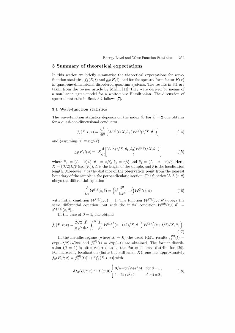
Energy-Level and Wave-Function Statistics 259
3 Summary of theoretical expectations
In this section we briefly summarise the theoretical expectations for wave-function statistics, fβ(E, t) and gβ(E, t), and for the spectral form factorK(τ)in quasi-one-dimensional disordered quantum systems. The results in 3.1 aretaken from the review article by Mirlin [11]; they were derived by means ofa non-linear sigma model for a white-noise Hamiltonian. The discussion ofspectral statistics in Sect. 3.2 follows [7].
3.1 Wave-function statistics
The wave-function statistics depends on the index β. For β = 2 one obtainsfor a quasi-one-dimensional conductor
f2(E, t;x) =d2
dt2
[W(1)(t/X, θ+)W(1)(t/X, θ−)
](14)
and (assuming |r| ≡ r ≫ ℓ)
g2(E, t;x)=−X d
dt
[W(2)(t/X, θ1, θ2)W(1)(t/X, θ−)
t
](15)
where θ+ = (L − x)/ξ, θ− = x/ξ, θ1 = r/ξ and θ2 = (L − x − r)/ξ. Here,X = (β/2)L/ξ (see [20]), L is the length of the sample, and ξ is the localisationlength. Moreover, x is the distance of the observation point from the nearestboundary of the sample in the perpendicular direction. The functionW(1)(z, θ)obeys the differential equation
∂
∂θW(1)(z, θ) =
(z2∂2
∂z2− z
)W(1)(z, θ) (16)
with initial condition W(1)(z, 0) = 1. The function W(2)(z, θ, θ′) obeys thesame differential equation, but with the initial condition W(2)(z, 0, θ) =zW(1)(z, θ).
In the case of β = 1, one obtains
f1(E, t;x) =2√
2
π√t
d2
dt2
∫ ∞
0
dz√zW(1)
((z+ t/2)/X, θ−
)W(1)
((z+ t/2)/X, θ+
).
(17)
In the metallic regime (where X → 0) the usual RMT results f(0)1 (t) =
exp(−t/2)/√
2πt and f(0)2 (t) = exp(−t) are obtained. The former distrib-
ution (β = 1) is often referred to as the Porter-Thomas distribution [29].For increasing localization (finite but still small X), one has approximately
fβ(E, t;x) = f(0)β (t)[1 + δfβ(E, t;x)] with
δfβ(E, t;x) ≃ P (x; 0)
3/4−3t/2+t2/4 forβ=1 ,
1−2t+t2/2 forβ=2 ,(18)
260 Bernhard Mehlig and Michael Schreiber
valid for t≪ X−1/2. Here P (x; t) is the one-dimensional diffusion propagator[30]. In the tails (t≫ X−1 > 1) of fβ(E, t;x), Eqs. (14,17) simplify to [15]
fβ(E, t;x) ≃ Aβ(x,X) exp(−2β√t/X) . (19)
This result may also be obtained within a saddle-point approximation to thenon-linear sigma model [16]. The prefactors Aβ(x,X) for β = 1, 2 are givenin [15,16].
We finally turn to the shape of the wave functions. In close vicinity of thelocalisation center, the anomalously localized wave functions exhibit a verynarrow peak (of width less than ℓ). The above expressions apply for r ≫ ℓand thus describe the smooth background intensity, but not the sharp peakitself [18]. For large values of t, for instance, it was suggested by Mirlin [18]that the background intensity should be given by
〈V |ψ(r)|2〉t ≈1
2
√tX
(1 + r
√t/(Lξ)
)−2
(20)
where in accordance with the above, ℓ≪ r is assumed, and also r ≪ ξ.It is necessary to emphasize that the tails of the wave-function amplitude
distribution [see for example (19)] may depend on the details of the modelconsidered. In the case of two-dimensional Anderson models at the centreof the spectrum, i.e. at E = 0, for instance, the distribution is of the formpredicted by the non-linear sigma model, albeit with modified coefficients [31].This could explain anomalies observed in simulations of two- and also in three-dimensional Anderson models [20,32–34]. In [35] the wave-function amplitudedistributions of random banded matrices near the band centre were analyzed.It was shown that they agree well with the predictions of the non-linear σmodel for the quasi-one-dimensional case [11,15].
In 4.1, results of exact diagonalisations of the quasi-one-dimensional An-derson tight-binding Hamiltonian are compared to (14,17-20).
3.2 Spectral statistics
The spectral two-point correlation function Rβ(E, ǫ) may be written as a sumof two contributions,
Rβ(E, ǫ) = Ravβ (E, ǫ) +Rosc
β (E, ǫ) . (21)
Ravβ (E, ǫ) is defined as
Ravβ (E, ǫ) =
∫dǫ′ v(ǫ− ǫ′)Rβ(E, ǫ) . (22)
Here v(ǫ) is a Gaussian window centred around zero with variance much largerthan the oscillations of Rβ(E, ǫ) in ǫ, and normalized to∆−1, see [7]. Rosc
β (E, ǫ)is the remaining oscillatory contribution.
Energy-Level and Wave-Function Statistics 261
The smooth contribution Ravβ (E, ǫ) describes correlations on energy scales
much larger than the mean level spacing and may be calculated within asemiclassical approach (using the diagonal approximation), diagrammatic per-turbation theory, or Dyson’s Brownian motion model. Rosc
β (E, ǫ) cannot becalculated in this way.
It was first demonstrated by Andreev and Altshuler [5] that there is a verysimple relation between smooth and oscillatory contributions to the spectralform factor. This relation describes non-universal deviations from RMT indisordered metals in terms of the spectral determinant Dβ(ǫ) of the diffusionpropagator P (x, t)
Ravβ (E, ǫ) = − 1
4π2
∂2
∂ǫ2log Dβ(ǫ) (23)
Roscβ (E, ǫ) =
1
π2cos(2πǫ/∆)D2
β(ǫ) . (24)
This relation implies in particular that non-universal corrections affect thetwo-point correlation function not only at large energy scales, but also atsmall scales (of the order of the mean level spacing). In [7] it was shown that(23,24) are a consequence of the fact that the two-point correlation functionis well approximated by a sum of shifted Gaussians.
For a quasi-one-dimensional diffusive conductor, the quantity Dβ(ǫ) in(23,24) is approximately given by Dβ(ǫ) = 4π2 exp[−2π2σ2
β(ǫ)/∆2] with
σ2β(ǫ) ≃ 2∆2
βπ2
[log(2πǫ) + sβ −
1
2
∞∑
ν=1
log(gν2/2)2
(gν2/2)2 + ǫ2
]. (25)
Here sβ is a β-dependent constant [7]. For the spectral form factor one obtains(see [11] and references quoted therein)
Kavβ (E, τ) =
2
β|τ |
∞∑
ν=0
e− πgν2|τ |
=2
β|τ |1
2+
1
2
∞∑
µ=−∞
e− πµ2/(g|τ |)√g|τ |
(26)
The asymptotic behaviour (for τ ≪ g−1 ≪ 1) is given by [4–6]
Kavβ (E, τ) =
2
β
√|τ |4g
(27)
and [5]
Koscβ (E, τ) =
∞∑
µ=1
(e−πgµ2|τ+1| + e−πgµ2|τ−1|
)(−1)µ 2
gµsinh(πµ). (28)
An alternative derivation of (28) was given in [7].In [22] these behaviours were compared to results of exact diagonalisations
of the quasi-one-dimensional Anderson tight-binding Hamiltonian. The resultsof [22] are summarized in Sect. 4.2.
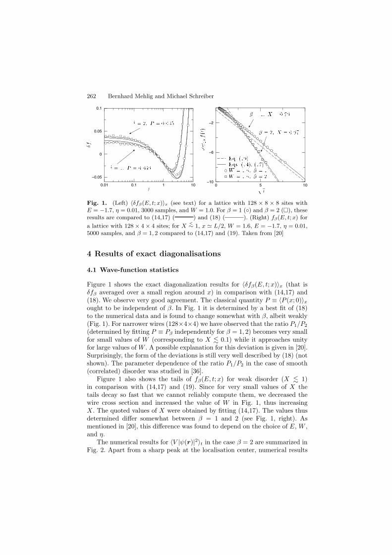
262 Bernhard Mehlig and Michael Schreiber
0 5 10−10
−6
−2
0.01 0.1 1 10
−0.05
0
0.05
0.1
Fig. 1. (Left) 〈δfβ(E, t; x)〉x (see text) for a lattice with 128 × 8 × 8 sites withE = −1.7, η = 0.01, 3000 samples, and W = 1.0. For β = 1 () and β = 2 (), theseresults are compared to (14,17) ( ) and (18) ( ). (Right) fβ(E, t; x) for
a lattice with 128 × 4 × 4 sites; for X<∼ 1, x ≃ L/2, W = 1.6, E = −1.7, η = 0.01,
5000 samples, and β = 1, 2 compared to (14,17) and (19). Taken from [20]
4 Results of exact diagonalisations
4.1 Wave-function statistics
Figure 1 shows the exact diagonalization results for 〈δfβ(E, t;x)〉x (that isδfβ averaged over a small region around x) in comparison with (14,17) and(18). We observe very good agreement. The classical quantity P ≡ 〈P (x; 0)〉xought to be independent of β. In Fig. 1 it is determined by a best fit of (18)to the numerical data and is found to change somewhat with β, albeit weakly(Fig. 1). For narrower wires (128×4×4) we have observed that the ratio P1/P2
(determined by fitting P ≡ Pβ independently for β = 1, 2) becomes very smallfor small values of W (corresponding to X 0.1) while it approaches unityfor large values ofW . A possible explanation for this deviation is given in [20].Surprisingly, the form of the deviations is still very well described by (18) (notshown). The parameter dependence of the ratio P1/P2 in the case of smooth(correlated) disorder was studied in [36].
Figure 1 also shows the tails of fβ(E, t;x) for weak disorder (X 1)in comparison with (14,17) and (19). Since for very small values of X thetails decay so fast that we cannot reliably compute them, we decreased thewire cross section and increased the value of W in Fig. 1, thus increasingX. The quoted values of X were obtained by fitting (14,17). The values thusdetermined differ somewhat between β = 1 and 2 (see Fig. 1, right). Asmentioned in [20], this difference was found to depend on the choice of E, W ,and η.
The numerical results for 〈V |ψ(r)|2〉t in the case β = 2 are summarized inFig. 2. Apart from a sharp peak at the localisation center, numerical results
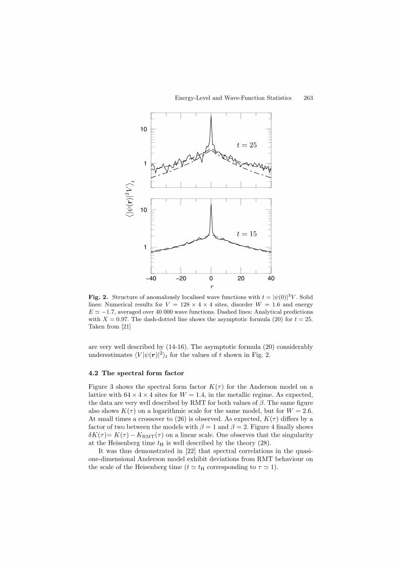
Energy-Level and Wave-Function Statistics 263
1
10
−40 −20 0 20 40
1
10
t = 15
t = 25
r
˙
|ψ(r
)|2V
¸
t
Fig. 2. Structure of anomalously localised wave functions with t = |ψ(0)|2V . Solidlines: Numerical results for V = 128 × 4 × 4 sites, disorder W = 1.6 and energyE ≃ −1.7, averaged over 40 000 wave functions. Dashed lines: Analytical predictionswith X = 0.97. The dash-dotted line shows the asymptotic formula (20) for t = 25.Taken from [21]
are very well described by (14-16). The asymptotic formula (20) considerablyunderestimates 〈V |ψ(r)|2〉t for the values of t shown in Fig. 2.
4.2 The spectral form factor
Figure 3 shows the spectral form factor K(τ) for the Anderson model on alattice with 64× 4× 4 sites for W = 1.4, in the metallic regime. As expected,the data are very well described by RMT for both values of β. The same figurealso shows K(τ) on a logarithmic scale for the same model, but for W = 2.6.At small times a crossover to (26) is observed. As expected, K(τ) differs by afactor of two between the models with β = 1 and β = 2. Figure 4 finally showsδK(τ)= K(τ)−KRMT(τ) on a linear scale. One observes that the singularityat the Heisenberg time tH is well described by the theory (28).
It was thus demonstrated in [22] that spectral correlations in the quasi-one-dimensional Anderson model exhibit deviations from RMT behaviour onthe scale of the Heisenberg time (t ≃ tH corresponding to τ ≃ 1).
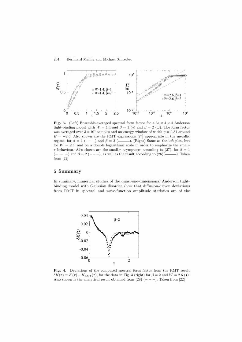
264 Bernhard Mehlig and Michael Schreiber
0 0.5 1 1.5 2 2.5τ
0
0.5
1
K(τ
)
W=1.4, β=1W=1.4, β=2
10−2 10−1 100 101
τ
10−2
10−1
100
K(τ
)
W=2.6, β=1W=2.6, β=2
Fig. 3. (Left) Ensemble-averaged spectral form factor for a 64 × 4 × 4 Andersontight-binding model with W = 1.4 and β = 1 () and β = 2 (). The form factorwas averaged over 3× 10⁴ samples and an energy window of width η = 0.31 aroundE = −2.6. Also shown are the RMT expressions [27] appropriate in the metallicregime, for β = 1 (- - - -) and β = 2 ( ). (Right) Same as the left plot, butfor W = 2.6, and on a double logarithmic scale in order to emphasize the small-τ behaviour. Also shown are the small-τ asymptotes according to (27), for β = 1(−·−·−) and β = 2 (−−−), as well as the result according to (26)( ). Takenfrom [22]
5 Summary
In summary, numerical studies of the quasi-one-dimensional Anderson tight-binding model with Gaussian disorder show that diffusion-driven deviationsfrom RMT in spectral and wave-function amplitude statistics are of the
0 2τ
-0.06
-0.04
-0.02
0
0.02
0.04
δK(τ
)
β=2
Times-ISOLatin1
Fig. 4. Deviations of the computed spectral form factor from the RMT resultδK(τ) ≡ K(τ)−KRMT(τ), for the data in Fig. 3 (right) for β = 2 and W = 2.6 (•).Also shown is the analytical result obtained from (28) (−−−). Taken from [22]
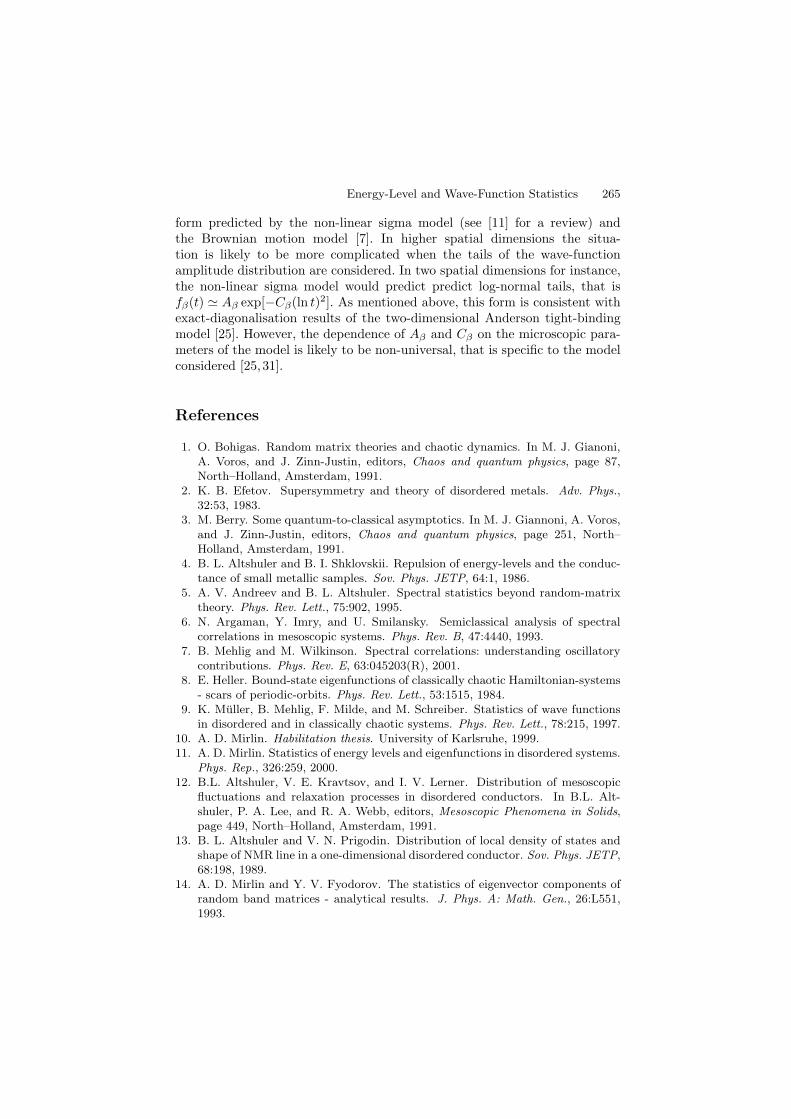
Energy-Level and Wave-Function Statistics 265
form predicted by the non-linear sigma model (see [11] for a review) andthe Brownian motion model [7]. In higher spatial dimensions the situa-tion is likely to be more complicated when the tails of the wave-functionamplitude distribution are considered. In two spatial dimensions for instance,the non-linear sigma model would predict predict log-normal tails, that isfβ(t) ≃ Aβ exp[−Cβ(ln t)2]. As mentioned above, this form is consistent withexact-diagonalisation results of the two-dimensional Anderson tight-bindingmodel [25]. However, the dependence of Aβ and Cβ on the microscopic para-meters of the model is likely to be non-universal, that is specific to the modelconsidered [25,31].
References
1. O. Bohigas. Random matrix theories and chaotic dynamics. In M. J. Gianoni,A. Voros, and J. Zinn-Justin, editors, Chaos and quantum physics, page 87,North–Holland, Amsterdam, 1991.
2. K. B. Efetov. Supersymmetry and theory of disordered metals. Adv. Phys.,32:53, 1983.
3. M. Berry. Some quantum-to-classical asymptotics. In M. J. Giannoni, A. Voros,and J. Zinn-Justin, editors, Chaos and quantum physics, page 251, North–Holland, Amsterdam, 1991.
4. B. L. Altshuler and B. I. Shklovskii. Repulsion of energy-levels and the conduc-tance of small metallic samples. Sov. Phys. JETP, 64:1, 1986.
5. A. V. Andreev and B. L. Altshuler. Spectral statistics beyond random-matrixtheory. Phys. Rev. Lett., 75:902, 1995.
6. N. Argaman, Y. Imry, and U. Smilansky. Semiclassical analysis of spectralcorrelations in mesoscopic systems. Phys. Rev. B, 47:4440, 1993.
7. B. Mehlig and M. Wilkinson. Spectral correlations: understanding oscillatorycontributions. Phys. Rev. E, 63:045203(R), 2001.
8. E. Heller. Bound-state eigenfunctions of classically chaotic Hamiltonian-systems- scars of periodic-orbits. Phys. Rev. Lett., 53:1515, 1984.
9. K. Muller, B. Mehlig, F. Milde, and M. Schreiber. Statistics of wave functionsin disordered and in classically chaotic systems. Phys. Rev. Lett., 78:215, 1997.
10. A. D. Mirlin. Habilitation thesis. University of Karlsruhe, 1999.11. A. D. Mirlin. Statistics of energy levels and eigenfunctions in disordered systems.
Phys. Rep., 326:259, 2000.12. B.L. Altshuler, V. E. Kravtsov, and I. V. Lerner. Distribution of mesoscopic
fluctuations and relaxation processes in disordered conductors. In B.L. Alt-shuler, P. A. Lee, and R. A. Webb, editors, Mesoscopic Phenomena in Solids,page 449, North–Holland, Amsterdam, 1991.
13. B. L. Altshuler and V. N. Prigodin. Distribution of local density of states andshape of NMR line in a one-dimensional disordered conductor. Sov. Phys. JETP,68:198, 1989.
14. A. D. Mirlin and Y. V. Fyodorov. The statistics of eigenvector components ofrandom band matrices - analytical results. J. Phys. A: Math. Gen., 26:L551,1993.
266 Bernhard Mehlig and Michael Schreiber
15. Y. V. Fyodorov and A. Mirlin. Statistical properties of eigenfunctions of randomquasi 1d one-particle Hamiltonians. Int. J. Mod. Phys. B, 8:3795, 1994.
16. V. I. Fal’ko and K. B. Efetov. Multifractality: generic property of eigenstates of2d disordered metals. Europhys. Lett., 32:627, 1995.
17. Y. V. Fyodorov and A. Mirlin. Mesoscopic fluctuations of eigenfunctions andlevel-velocity distribution in disordered metals. Phys. Rev. B, 51:13403, 1995.
18. A. D. Mirlin. Spatial structure of anomalously localized states in disorderedconductors. J. Math. Phys., 38:1888, 1997.
19. J. Cullum and R. A. Willoughby. Lanczos Algorithms for Large SymmetricEigenvalue Computations. Birkhauser, Boston, 1985.
20. V. Uski, B. Mehlig, R. Romer, and M. Schreiber. Exact diagonalization studyof rare events in disordered conductors. Phys. Rev. B, 62:R7699, 2000.
21. V. Uski, B. Mehlig, and M. Schreiber. Spatial structure of anomalously localizedstates in disordered conductors. Phys. Rev. B, 66:233104, 2002.
22. V. Uski, B. Mehlig, and M. Wilkinson. Unpublished.23. M. Wilkinson. Random matrix theory in semiclassical quantum mechanics of
chaotic systems. J. Phys. A: Math. Gen., 21:1173, 1988.24. M. Wilkinson and P. N. Walker. A Brownian motion model for the parameter
dependence of matrix elements. J. Phys. A: Math. Gen., 28:6143, 1996.25. V. Uski, B. Mehlig, R. Romer, and M. Schreiber. Smoothed universal correla-
tions in the two-dimensional Anderson model. Phys. Rev. B, 59:4080, 1999.26. P. W. Anderson. Absence of diffusion in certain random lattices. Phys. Rev.,
109:1492, 1958.27. M. L. Mehta. Random Matrices and the Statistical Theory of Energy Levels.
Academic Press, New York, 1991.28. W. T. Vetterling W. H. Press, S. A. Teukolsky and B. P. Flannery. Numerical
recipes. Cambridge University Press, Cambridge, 1992.29. C. E. Porter. Fluctuations of quantal spectra. In C. E. Porter, editor, Statistical
Theories of Spectra, page 2. Academic Press, New York, 1965.30. N. G. van Kampen. Stochastic processes in physics and chemistry. North-
Holland, Amsterdam, 1983.31. V. M. Apalkov, M. E. Raikh, and B. Shapiro. Anomalously localized states in
the Anderson model. Phys. Rev. Lett., 92:066601, 2004.32. V. Uski, B. Mehlig, R.A. Romer, and M. Schreiber. Incipient localization in the
Anderson model. Physica B, 284 - 288:1934, 2000.33. B. K. Nikolic. Statistical properties of eigenstates in three-dimensional meso-
scopic systems with off-diagonal or diagonal disorder. Phys. Rev. B, 64:014203,2001.
34. B. K. Nikolic. Quest for rare events in mesoscopic disordered metals. Phys. Rev.B, 65:012201, 2002.
35. V. Uski, R. A. Romer, and M. Schreiber. Numerical study of eigenvector sta-tistics for random banded matrices. Phys. Rev. E, 65:056204, 2002.
36. V. Uski, B. Mehlig, and M. Schreiber. Signature of ballistic effects in disorderedconductors. Phys. Rev. B, 63:241101, 2001.
Fine Structure of the Integrated Densityof States for Bernoulli–Anderson Models
Peter Karmann1, Rudolf A. Romer2, Michael Schreiber1, and PeterStollmann3
1 Technische Universitat Chemnitz, Institut fur Physik09107 Chemnitz, Germany
2 Department of Physics and Centre for Scientific Computing,University of Warwick, Coventry, CV4 7AL, United Kingdom
3 Technische Universitat Chemnitz, Fakultat fur Mathematik09107 Chemnitz, Germany
1 Introduction
Disorder is one of the fundamental topics in science today. A very prominentexample is Anderson’s model [1] for the transition from metal to insulatorunder the presence of disorder.
Apart from its intrinsic physical value this model has triggered an enor-mous amount of research in the fields of random operators and numericalanalysis, resp. numerical physics. As we will explain below, the Andersonmodel poses extremely hard problems in these fields and so mathematicalrigorous proofs of many well substantiated findings of theoretical physics arestill missing. The very nature of the problem also causes highly nontrivialchallenges for numerical studies.
The transition mentioned above can be reformulated in mathematicalterms in the following way: for a certain random Hamiltonian one has toprove that its spectral properties change drastically as the energy varies. Forlow energies there is pure point spectrum, with eigenfunctions that decayexponentially. This energy regime is called localization.
For energies away from the spectral edges, the spectrum is expected to beabsolutely continuous, providing for extended states that can lead to trans-port. Sadly enough, more or less nothing has been proven concerning thesecond kind of spectral regime, called delocalization. An exception are resultson trees [2, 3], and for magnetic models [4]. Anyway, there are convincingtheoretical arguments and numerical results that support the picture of themetal–insulator transition (which is, in fact, a dimension-dependent effect andshould take place for dimensions d > 2).
In our research we are dealing with a different circle of questions. TheAnderson model is in fact a whole class of models: an important input is the
268 Peter Karmann et al.
measure µ that underlies the random onsite couplings. In all proofs of localiza-tion (valid for d > 1) one needs regularity of this measure µ. This excludes aprominent and attractive model: the Anderson model of a binary alloy, i.e. twokinds of atoms randomly placed on the sites of a (hyper)cubic lattice, knownas Bernoulli–Anderson model in the mathematical community. Basically thereare two methods of proof for localization: multiscale analysis [5], and the frac-tional moment method [6]. In both cases one needs an a-priori bound on theprobability that eigenvalues of certain Hamiltonians cluster around a fixedenergy, i.e., one has to exclude resonances of finite box Hamiltonians. Equiva-lently, one needs a weak kind of continuity of the integrated density of states(IDS). In multiscale analysis this a-priori estimate comes in a form that isknown as Wegner’s estimate [7]. Here we will present both rigorous analyticalresults and numerical studies of these resonances. We will take some time andeffort to describe the underlying concepts and ideas in the next Section. Thenwe report recent progress concerning analytical results. Here one has to men-tion a major breakthrough obtained in a recent paper [8] of J. Bourgain andC. Kenig who prove localization for the continuum Bernoulli–Anderson modelin dimensions d ≥ 2. Finally, we display our numerical studies and commenton future directions of research.
We conclude this section with an overview over recent contributions in thephysics literature concerning the binary-alloy model. These may be classifiedinto mainly simulations or mainly theoretical analyses. The former are dis-cussed in [9], albeit in the restricted setting of a Bethe lattice, providing a de-tailed analysis of the electronic structure of the binary-alloy and the quantum-percolation model, which can be derived from the binary alloy replacing oneof the alloy constituents by vacancies. The study is based on a selfconsistentscheme for the distribution of local Green’s functions. Detailed results for thelocal density of states (DOS) are obtained, from which the phase diagramof the binary alloy is constructed. The existence of a quantum-percolationthreshold is discussed. Another study [10] of the quantum site-percolationmodel on simple cubic lattices focuses on the statistics of the local DOS andthe spatial structure of the single particle wave functions. By using the kernelpolynomial previous studies of the metal–insulator transition are refined andthe nonmonotonic energy dependence of the quantum-percolation thresholdis demonstrated. A study of the three-dimensional binary-alloy model withadditional disorder for the energy levels of the alloy constituents is presentedin [11]. The results are compared with experimental results for amorphousmetallic alloys. By means of the transfer-matrix method, the metal–insulatortransitions are identified and characterized as functions of Fermi-level posi-tion, band broadening due to disorder and alloy composition. The latter isalso investigated in [12], which discusses the conditions to be put on mean-field-like theories to be able to describe fundamental physical phenomena indisordered electron systems. In particular, options for a consistent mean-fieldtheory of electron localization and for a reliable description of transport prop-erties are investigated. In [13] the single-site coherent potential approximation
Fine Structure of the Integrated DOS for Bernoulli–Anderson Models 269
is extended to include the effects of non-local disorder correlations (i.e. alloyshort-range order) on the electronic structure of random alloy systems. Thisis achieved by mapping the original Anderson disorder problem to that ofa selfconsistently embedded cluster. The DOS of the binary-alloy model hasbeen studied in [14], where also the mobility edge, i.e. the phase boundarybetween metallic and insulating behaviour was investigated. The critical be-haviour, in particular the critical exponent with which the localization lengthof the electronic states diverges at the phase transition was analyzed in [15]in comparison with the standard Anderson model.
2 Resonances and the integrated density of states
2.1 Wegner estimates, IDS, and localization
In this Section we sketch the basic problem and introduce the model we wantto consider. A major point of the rather expository style is to make clear, whythe problem is as difficult as it appears to be. This also sheds some light onwhy it is intrinsically hard to study numerically. Let us first write down theHamiltonian in an analyst’s notation:
On the Hilbert space ℓ2(Zd) we consider the random operator
H(ω) = −∆+ Vω,
where the discrete Laplacian incorporates the constant (nonrandom) off-diagonal or hopping terms. It is defined, for ψ ∈ ℓ2(Zd) by
∆ψ(i) =∑
〈i,j〉
ψ(j)
for i ∈ Zd. The notation reflects 〈·, ·〉 that we are dealing with a nearest neigh-
bor interaction, where the value of the wave function at site i is only influencedby those at the 2 d neighbors on the integer lattice. Here we neglect the di-agonal part ψ(i) which would only contribute a shift of the energy scale. Therandom potential Vω is, in its simplest form, given by independent identicallydistributed (short: i.i.d.) random variables at the different sites. A convenientrepresentation is given in the following way:
Ω =∏
i∈Zd
R, P =∏
i∈Zd
µ, Vω(i) = ωi
where µ is a probability measure on the real line. This function Vω(i) givesthe random diagonal multiplication operator acting as
Vωψ(i) = ωiψ(i).
For simplicity we assume that the support of the so-called single-site measureµ is a compact setK ⊂ R. Put differently, for every site i we perform a random
270 Peter Karmann et al.
experiment that gives the value ωi distributed according to µ. In physicist’snotation we get
H(ω) =∑
〈i,j〉
|i〉〈j|+∑
i
ωi|i〉〈i|,
where |i〉 denotes the basis functions in site representation.In principle, one expects that the spectral properties should not depend
too much on the specific distribution µ (apart from the very special case thatµ reduces to a point mass, in which case there is no disorder present). Let ustake a look at two very different cases. In the Bernoulli–Anderson model wehave the single-site measure µ = 1
2δ0 + 12δ1. In that case the value ωi ∈ 0, 1
is determined by a fair coin. We will also consider a coupling parameter W inthe random part, in which case we have either ωi = 0 or ωi = W each withprobability 1
2 . The resulting random potential is denoted by V Bω . In the second
case the potential value is determined with respect to the uniform distributionso that we get µ(dx) = χ[0,1](x)dx. We write V U
ω for this case.Let us point out one source of the complexity of the problem: The two
operators that sum up to H(ω) are of very different nature:
• The discrete Laplacian is a difference operator. It is diagonal in Fourierspace L2([0, 2π]d), where it is given by multiplication with the function
d∑
k=1
2 cosxk.
Therefore, its spectrum is given by the range of this function, so that
σ(−∆) = [−2d, 2d],
the spectrum being purely absolutely continuous.• The random multiplication operator Vω is diagonal in the basis δi|i ∈ Z
d.The spectrum is hence the closure of the range of Vω, which is just thesupport K of the measure for P–a.e.ω ∈ Ω (a.e. stands for almost every,i.e., for all but a set of measure zero). In the aforementioned special caseswe get
σ(V Bω ) = 0, 1
for the Bernoulli–Anderson model and
σ(V Uω ) = [0, 1],
both for a.e. ω ∈ Ω. Clearly, the spectral type is pure point with perfectlylocalized eigenfunctions for every ω, the set of eigenvalues being given byωi|i ∈ Z
d.One major problem of the analysis as well as the numerics is now obvious:We add two operators of the same size with completely different spectral typeand there is no natural basis to diagonalize the sum H(ω) = −∆+ Vω, since
Fine Structure of the Integrated DOS for Bernoulli–Anderson Models 271
one of the two terms is diagonal in position space while the other is diagonalin momentum space (the Fourier picture).
Another cause of difficulties is the expected spectral type of H(ω). Inthe localized regime it has a dense set of eigenvalues. These eigenvalues areextremely unstable. Rank-one perturbation theory gives the following factwhich illustrates this instability: If we fix all values ωj except one, say ωi andvary the latter continuously in an interval, the resulting spectral measureswill be mutually singular and for a dense set of values of ωi the spectrum willcontain a singular continuous component, cf. [16].
Moreover, the qualitative difference between the Bernoulli–Anderson modeland the model with uniform distribution is evident: V U
ω displays the spectraltype we want to prove for H(ω): it has a dense set of eigenvalues for a.e. ω. Ifone can treat −∆ in some sense as a small perturbation we arrive at the de-sired conclusion. In view of the preceding paragraph, this cannot be achievedby standard perturbation arguments. In the Bernoulli–Anderson model V B
ω
has only eigenvalues 0 and 1, each infinitely degenerate.In typical proofs of localization an important tool is the study of box
Hamiltonians. To explain this, we consider the cube ΛL(i) of side length Lcentered at i. We restrict H(ω) to the sites in ΛL(i) which constitutes asubspace of dimension |ΛL(i)| = Ld. We denote the restriction by HL(ω) andsuppress the boundary condition, since it does not play a role in asymptoticproperties as L→∞.
These box Hamiltonians enter in resolvent expansions and it is importantto estimate the probability that their resolvents have a large norm, i.e., we aredealing here with small-denominator problems. Since the resolvent has largenorm for energies near the spectrum one needs upper bounds for
Pσ(HL(ω)) ∩ [E − ǫ, E + ǫ] = ∅ = p(ǫ, L).
In fact, one wants to show that p(ǫ, L) is small for large L and small ǫ. At thesame time, there is a clear limitation to such estimates: In the limit L → ∞the spectra of HL(ω) converge to the spectrum of H(ω). This means that forfixed ǫ > 0 and E ∈ σ(H(ω)) (and only those energies E are of interest),
p(ǫ, L)→ 1 for L→∞.
The famous Wegner estimate [7] states that for absolutely continuous µ weget
p(ǫ, L) ≤ CǫLd, (1)
where the last factor is the volume of the cube |ΛL(i)| = Ld. This estimate issufficient for a proof of localization for energies near the spectral edges. Theproof is not too complicated for the discrete model. To see why it might betrue, let us include a very simple argument in the case that there is no hoppingterm.
Then
272 Peter Karmann et al.
Pσ(Vω) ∩ [E − ǫ, E + ǫ] = ∅ = P∃j ∈ ΛL s.t. Vω(j) ∈ [E − ǫ, E + ǫ]≤ |ΛL| · µ[E − ǫ, E + ǫ]
≤ C · |ΛL| · ǫ,
if µ is absolutely continuous. Here we see that the situation is completelydifferent for the Bernoulli–Anderson model for which µ[E − ǫ, E + ǫ] ≥ 1
2whenever E ∈ 0, 1. Also, it is clear that a Wegner estimate of the type (1)above cannot hold. Since in
Pσ(HL(ω)) ∩ [E − ǫ, E + ǫ] = ∅
only 2|ΛL| Bernoulli variables are comprised, this probability must at least be2−|ΛL|, unless it vanishes.
The Wegner estimate is intimately related to continuity properties of theintegrated density of states (IDS), a function N : R → [0,∞) that measuresthe number of energy levels per unit volume:
N(E) = limL→∞
1
|ΛL|E(Trχ(−∞,E](HL(ω))).
Here E denotes the expectation value and χ(−∞,E](HL(ω)) is the projectiononto the eigenspace spanned by the eigenvectors with eigenvalue below Eand the trace determines the dimension of this space, i.e., the number ofeigenvalues below E counted with their multiplicity. Since we are dealing withoperators of rank at most |ΛL|, we get
N(E + ǫ)−N(E − ǫ) ≈ 1
|ΛL|E(Trχ(E−ǫ,E+ǫ](HL(ω)))
≤ Pσ(HL(ω)) ∩ [E − ǫ, E + ǫ] = ∅.
This means that Wegner estimates lead to continuity of the IDS. Althoughthat is not clear from the above rather crude reasoning, the Wegner estimatefor absolutely continuous µ yields differentiability of the IDS.
2.2 Recent rigorous analytical results
In this section we will mainly be dealing with continuum models,
H(ω) = −∆+ Vω,
where −∆ is now the unbounded Laplacian with domain W 2,2(Rd), theSobolev space of square integrable functions with square integrable secondpartial derivatives. The random multiplication operator Vω is defined by
Vω(x) =∑
i∈Zd
ωiu(x− i),
Fine Structure of the Integrated DOS for Bernoulli–Anderson Models 273
with a single-site potential u(x) ≥ 0 bounded and of compact support (forsimplicity reasons), and random coupling like above. Some results we mentionare valid under more general assumptions, as can be seen in the original papers.For results concerning localization of these models we refer to [5] for a surveyof the literature up to the year 2000. More recent results concerning the IDSand its continuity properties can be found in [17]. Here we will report on morerecent developments. The first result is partly due to one of us [18].
Theorem 1. Let H(ω) be an alloy-type model and u ≥ κχ[−1/2,1/2]d for somepositive κ. Then for each E0 ∈ R there exists a constant CW such that, for allE ≤ E0 and ε ≤ 1/2
ETr[χ[E−ε,E+ε](HL(ω))] ≤ CW s(µ, ε) (log 1ε )d |ΛL|, (2)
wheres(µ, ε) = supµ([E − ε,E + ε]) | E ∈ R. (3)
The mentioned alloy-type models include the models we introduced aswell as additional periodic exterior potentials and magnetic vector potentials.The idea of the proof is to combine methods from [19] with a technique tocontrol the influence of the kinetic term: the estimate in [19] is quadratic in thevolume of the cube and so it cannot be used to derive continuity of the IDS.On the other hand, there had been recent progress for models with absolutelycontinuous µ [20–22] using the spectral shift function. In [18] we present animproved estimate of the spectral shift function and apply it to arrive at theestimate (2). Of course, the latter is not really helpful, unless the measure µshares a certain continuity. Still it is interesting in so far that it yields that Nis nearly as continuous as µ with a logarithmically small correction. For moredetails we refer to [18], where the reader can also find a detailed account ofhow our result compares with recent results in this direction.
We now mention a major breakthrough obtained in the recent work [8]where the continuum Bernoulli–Anderson model is treated. For this model,the authors set up a multi-scale induction to prove a Wegner estimate of thefollowing type:
Theorem 2. For the Bernoulli–Anderson model and α, β > 0 there existC, γ > 0 such that
Pσ(HL(ω)) ∩ [E − ǫ, E + ǫ] = ∅ ≤ CL− 12 d+α
forǫ ≤ exp(−γL 4
3+β).
This can be found as Lemma 5.1 in [8]. It is important to note that the proofdoes not so far extend to the discrete case. The reason is that a major step inthe proof is a quantitative unique continuation result that does not extend tothe discrete setting. Therefore, Wegner estimates for the discrete Bernoulli–Anderson model are still missing.
274 Peter Karmann et al.
3 Numerical studies
Most numerical studies have been performed for the standard Anderson modelof localization with uniform distribution of the potential values. In this modelthe DOS changes smoothly with increasing disorder from the DOS of theLaplacian with its characteristic van Hove singularities to one featurelessband [23]. If the distribution is chosen as usual with mean 0 and width W,then the theoretical band edges are given by ±(2d +W /2). Numerically thesevalues are of course reached with vanishing probability. If the box distributionis replaced by an unbounded distribution like the Gaussian or the Lorentzian,then the band tails in principle extend to infinity, although numerically nosignificant change can be observed from the box-distribution case [24]. A dra-matically different situation occurs in a binary alloy, where with increasingdisorder W the DOS separates into two bands of width 4 d each. Choosingthe measure µ = 1
2δ0 + 12δW as discussed in the previous section, the split-
ting of the band into subbands occurs theoretically for W = 4 d, although theagain numerically very small DOS in the tails of the subbands leads to the ap-pearance of separated subbands already for smaller disorder values [14]. This,however, is not the topic of the current investigation. We rather concentrateon unexpected structures that we have found near the centre of the subbands.
The DOS is defined as usual
ρ(E) =
⟨ Ld∑
i=1
δ(E − Ei)
⟩
where Ei are the eigenvalues of the box Hamiltonian discussed in the previoussection, and 〈· · · 〉 indicates the average over an ensemble of different configu-rations of the random potential, i.e. the disorder average. For the numericaldiagonalization we use the Lanczos algorithm [25] which is very effective forsparse matrices. In the present case the matrices are extremely sparse, be-cause except for the diagonal matrix element with the potential energy thereare only 2 d elements in each row and column of the secular matrix due to theLaplacian. In fact, for the standard model of Anderson localization which is ofcourse as sparse as the Bernoulli–Anderson Hamiltonian matrix the Lanczosalgorithm has been shown to be most effective also in comparison with moremodern eigenvalue algorithms [26, 27]. One of the reasons for the difficultieswhich all eigenvalue algorithms encounter is our use of periodic boundaryconditions in all directions, making a transformation of the secular matrix toa band matrix impossible. However, a severe problem arises for the Lanczosalgorithm, because numerical inaccuracies due to finite precision arithmeticsyield spurious eigenvalues which show up as incorrectly multiple eigenener-gies. In principle these can be detected and eliminated in a straightforwardway. The respective procedure, however, becomes ineffective in those partsof the spectrum where the Hamiltonian itself has multiple eigenvalues or anunusually large DOS. This happens to be the case in our investigation and
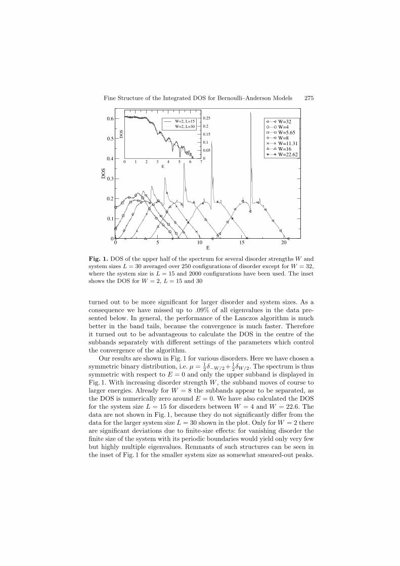
Fine Structure of the Integrated DOS for Bernoulli–Anderson Models 275
0 5 10 15 20E
0
0.1
0.2
0.3
0.4
0.5
0.6
DO
S
W=32W=4W=5.65W=8W=11.31W=16W=22.62
0 1 2 3 4 5 6 7E
0
0.05
0.1
0.15
0.2
0.25D
OS
W=2, L=15
W=2, L=30
Fig. 1. DOS of the upper half of the spectrum for several disorder strengths W andsystem sizes L = 30 averaged over 250 configurations of disorder except for W = 32,where the system size is L = 15 and 2000 configurations have been used. The insetshows the DOS for W = 2, L = 15 and 30
turned out to be more significant for larger disorder and system sizes. As aconsequence we have missed up to .09% of all eigenvalues in the data pre-sented below. In general, the performance of the Lanczos algorithm is muchbetter in the band tails, because the convergence is much faster. Thereforeit turned out to be advantageous to calculate the DOS in the centre of thesubbands separately with different settings of the parameters which controlthe convergence of the algorithm.
Our results are shown in Fig. 1 for various disorders. Here we have chosen asymmetric binary distribution, i.e. µ = 1
2δ−W/2+ 12δW/2. The spectrum is thus
symmetric with respect to E = 0 and only the upper subband is displayed inFig. 1. With increasing disorder strength W , the subband moves of course tolarger energies. Already for W = 8 the subbands appear to be separated, asthe DOS is numerically zero around E = 0. We have also calculated the DOSfor the system size L = 15 for disorders between W = 4 and W = 22.6. Thedata are not shown in Fig. 1, because they do not significantly differ from thedata for the larger system size L = 30 shown in the plot. Only forW = 2 thereare significant deviations due to finite-size effects: for vanishing disorder thefinite size of the system with its periodic boundaries would yield only very fewbut highly multiple eigenvalues. Remnants of such structures can be seen inthe inset of Fig. 1 for the smaller system size as somewhat smeared-out peaks.
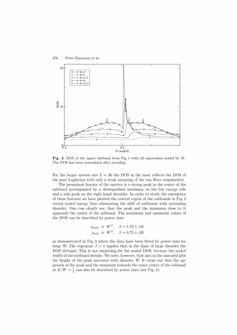
276 Peter Karmann et al.
0.4 0.5E (scaled)
0
10
20
DO
S
W=32W=8W=11.31W=16W=22.62
Fig. 2. DOS of the upper subband from Fig. 1 with all eigenvalues scaled by W .The DOS has been normalized after rescaling
For the larger system size L = 30 the DOS in the inset reflects the DOS ofthe pure Laplacian with only a weak smearing of the van Hove singularities.
The prominent feature of the spectra is a strong peak in the centre of thesubband accompanied by a distinguished minimum on the low energy sideand a side peak on the right hand shoulder. In order to study the emergenceof these features we have plotted the central region of the subbands in Fig. 2versus scaled energy thus eliminating the shift of subbands with increasingdisorder. One can clearly see, that the peak and the minimum close to itapproach the centre of the subband. The maximum and minimum values ofthe DOS can be described by power laws
ρmax ∝ W β , β = 1.79± .03
ρmin ∝ W β , β = 0.75± .03
as demonstrated in Fig. 3 where the data have been fitted by power laws forlarge W. The exponent β > 1 implies that in the limit of large disorder theDOS diverges. This is not surprising for the scaled DOS, because the scaledwidth of the subband shrinks. We note, however, that also in the unscaled plotthe height of the peak increases with disorder W. It turns out that the ap-proach of the peak and the minimum towards the exact centre of the subbandat E/W = 1
2 can also be described by power laws (see Fig. 4):
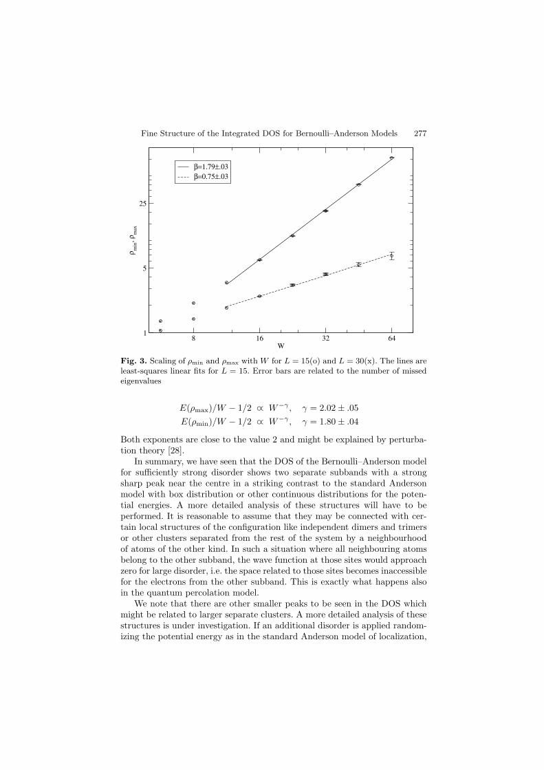
Fine Structure of the Integrated DOS for Bernoulli–Anderson Models 277
8 16 32 64W
1
5
25
ρm
in,
ρm
ax
β=1.79±.03
β=0.75±.03
Fig. 3. Scaling of ρmin and ρmax with W for L = 15(o) and L = 30(x). The lines areleast-squares linear fits for L = 15. Error bars are related to the number of missedeigenvalues
E(ρmax)/W − 1/2 ∝ W−γ , γ = 2.02± .05
E(ρmin)/W − 1/2 ∝ W−γ , γ = 1.80± .04
Both exponents are close to the value 2 and might be explained by perturba-tion theory [28].
In summary, we have seen that the DOS of the Bernoulli–Anderson modelfor sufficiently strong disorder shows two separate subbands with a strongsharp peak near the centre in a striking contrast to the standard Andersonmodel with box distribution or other continuous distributions for the poten-tial energies. A more detailed analysis of these structures will have to beperformed. It is reasonable to assume that they may be connected with cer-tain local structures of the configuration like independent dimers and trimersor other clusters separated from the rest of the system by a neighbourhoodof atoms of the other kind. In such a situation where all neighbouring atomsbelong to the other subband, the wave function at those sites would approachzero for large disorder, i.e. the space related to those sites becomes inaccessiblefor the electrons from the other subband. This is exactly what happens alsoin the quantum percolation model.
We note that there are other smaller peaks to be seen in the DOS whichmight be related to larger separate clusters. A more detailed analysis of thesestructures is under investigation. If an additional disorder is applied random-izing the potential energy as in the standard Anderson model of localization,
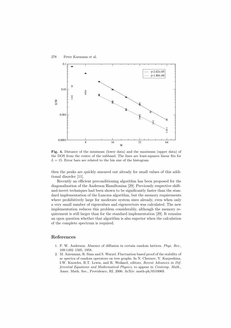
278 Peter Karmann et al.
8 16 32 64W
0.0001
0.001
0.01
0.1
E/W
γ=2.02±.05γ=1.80±.04
Fig. 4. Distance of the minimum (lower data) and the maximum (upper data) ofthe DOS from the centre of the subband. The lines are least-squares linear fits forL = 15. Error bars are related to the bin size of the histogram
then the peaks are quickly smeared out already for small values of this addi-tional disorder [11].
Recently an efficient preconditioning algorithm has been proposed for thediagonalization of the Anderson Hamiltonian [29]. Previously respective shift-and-invert techniques had been shown to be significantly faster than the stan-dard implementation of the Lanczos algorithm, but the memory requirementswhere prohibitively large for moderate system sizes already, even when onlya very small number of eigenvalues and eigenvectors was calculated. The newimplementation reduces this problem considerably, although the memory re-quirement is still larger than for the standard implementation [29]. It remainsan open question whether that algorithm is also superior when the calculationof the complete spectrum is required.
References
1. P. W. Anderson. Absence of diffusion in certain random lattices. Phys. Rev.,109:1492–1505, 1958.
2. M. Aizenman, R. Sims and S. Warzel. Fluctuation based proof of the stability ofac spectra of random operators on tree graphs. In N. Chernov, Y. Karpeshina,I.W. Knowles, R.T. Lewis, and R. Weikard, editors, Recent Advances in Dif-ferential Equations and Mathematical Physics, to appear in Contemp. Math.,Amer. Math. Soc., Providence, RI, 2006. ArXiv: math-ph/0510069.
Fine Structure of the Integrated DOS for Bernoulli–Anderson Models 279
3. A. Klein. Absolutely continuous spectrum in the Anderson model on the Bethelattice. Math. Res. Lett. 1, 4:399–407, 1994.
4. F. Germinet, A. Klein, J. Schenker: announced.5. P. Stollmann. Caught by disorder: bound states in random media. Progress in
Mathematical Physics, Vol. 20. Birkhauser, Boston, 2001.6. M. Aizenman, A. Elgart, S. Naboko, J. Schenker, G. Stolz. Moment analysis
for localization in random Schrodinger operators. ArXiv: math-ph/0308023.Invent. Math., 163:343–413, 2006.
7. F. Wegner. Bounds on the DOS in disordered systems. Z. Phys. B, 44:9–15,1981.
8. J. Bourgain and C. Kenig. Localization for the Bernoulli–Anderson model.Invent. Math., 161:389–426, 2005.
9. A. Alvermann and H. Fehske. Local distribution approach to the electronicstructure of binary alloys. Eur. Phys. J. B, 48:295–303, 2005. ArXiv: cond-mat/0411516.
10. G. Schubert, A. Weiße and H. Fehske. Localization effects in quantum perco-lation. Phys. Rev. B, 71:045126, 2005.
11. I. V. Plyushchay, R. A. Romer and M. Schreiber. Three-dimensional Andersonmodel of localization with binary random potential. Phys. Rev. B, 68:064201,2003.
12. V. Janis and J. Kolorenc. Mean-field theories for disordered electrons: Diffusionpole and Anderson localization. Phys. Rev. B, 71:245106, 2005. ArXiv: cond-mat/0501586.
13. M. S. Laad and L. Craco. Cluster coherent potential approximation for elec-tronic structure of disordered alloys. J. Phys.: Condens. Matter, 17:4765–4777,2005. ArXiv: cond-mat/0409031.
14. C. M. Soukoulis, Q. Li, and G. S. Grest. Quantum percolation in three-dimensional systems. Phys. Rev. B, 45:7724–7729, 1992.
15. E. Hofstetter and M. Schreiber. Finite-size scaling and critical exponents: Anew approach and its application to Anderson localization. Europhys. Lett.,27:933–939, 1993.
16. B. Simon. Spectral analysis of rank one perturbations and applications. Math-ematical quantum theory. II. Schrodinger operators (Vancouver, BC, 1993),CRM Proc. Lecture Notes Vol. 8 :109–149. Amer. Math. Soc., Providence, RI,1995.
17. I. Veselic. Integrated density of states and Wegner estimates for randomSchrodinger operators. In C. Villegas-Blas and R. del Rio, editors, Schrodingeroperators (Universidad Nacional Autonoma de Mexico, 2001), volume 340of Contemp. Math., pages 98–184. Amer. Math. Soc., Providence, RI, 2004.ArXiv: math-ph/0307062.
18. D. Hundertmark, R. Killip, S. Nakamura, P. Stollmann, I. Veselic: Boundson the spectral shift function and the density of states. Comm. Math. Phys.,262:489–503, 2006.
19. P. Stollmann. Wegner estimates and localization for continuum Anderson mod-els with some singular distributions. Arch. Math. (Basel), 75:307–311, 2000.
20. J.-M. Combes, P. D. Hislop, and F. Klopp. Holder continuity of the integrateddensity of states for some random operators at all energies. Int. Math. Res.Not., 4:179–209, 2003.
280 Peter Karmann et al.
21. J.-M. Combes, P. D. Hislop, F. Klopp, and S. Nakamura. The Wegner estimateand the integrated density of states for some random operators. Proc. IndianAcad. Sci. Math. Sci., 112:31–53, 2002. www.ias.ac.in/mathsci/.
22. J.-M. Combes, P. D. Hislop, and S. Nakamura. The Lp-theory of the spectralshift function, the Wegner estimate, and the integrated density of states forsome random Schrodinger operators. Commun. Math. Phys., 70:113–130, 2001.
23. A. Croy, R. A. Romer and M. Schreiber. Localization of electronic statesin amorphous materials: recursive Green’s function method and the metal–insulator transition at E = 0. In K. H. Hoffmann and A. Meyer, editors, Par-allel Algorithms and Cluster Computing - Implementions, Algorithm and Ap-plications, Lecture Notes in Computational Science and Engineering. Springer,Berlin, 2006.
24. B. Bulka, M. Schreiber and B. Kramer. Localization, quantum interference,and the metal–insulator transition. Z. Phys. B, 66:21–30, 1987.
25. J. K. Cullum and R. A. Willoughby. Lanczos Algorithms for Large SymmetricEigenvalues Computations, Vol. 1, Theory. Birkhauser, Basel, 1985.
26. U. Elsner, V. Mehrmann, F. Milde, R. A. Romer and M. Schreiber. The Ander-son model of localization: A challenge for modern eigenvalue methods. SIAMJ. Sci. Comp., 20:2089–2102, 1999.
27. M. Schreiber, F. Milde, R. A. Romer, U. Elsner and V. Mehrmann. Electronicstates in the Anderson model of localization: benchmarking eigenvalue algo-rithms. Comp. Phys. Comm., 121-122:517–523, 1999.
28. V. Z. Cerovski. (private communication).29. O. Schenk, M. Bollhofer and R. A. Romer. On large scale diagonalization
techniques for the Anderson model of localization. ArXiv: math.NA/0508111.
Modelling Aging Experiments in Spin Glasses
Karl Heinz Hoffmann1, Andreas Fischer1, Sven Schubert1, and ThomasStreibert1,2
1 Technische Universitat Chemnitz, Institut fur Physik09107 Chemnitz, [email protected]
[email protected] T. Streibert has also published as T. Klotz
1 Introduction
Spin glasses are a paradigm for complex systems. They show a wealth ofdifferent phenomena including metastability and aging. Especially in the lowtemperature regime they reveal a very complex dynamical behaviour. Fortemperatures below the spin glass transition temperature one finds a varietyof features connected to the inability of the systems to attain thermodynamicequilibrium with the ambient conditions on the observation time scale: agingand memory effects have been observed in many experiments [1–11]. Spinglasses are good model systems as their magnetism provides an easy andvery accurate experimental probe into their dynamic behavior. In order toinvestigate such features different experimental techniques have been applied.Complicated setups including temperature and field changes with subsequentrelaxation phases lead to more interesting effects such as age reinitializationand freezing [12,13].
In order to understand the observed phenomena a number of differentconcepts have been advanced. They include real space models, such as thedroplet model [14–17], mean field theory approaches [18–21], as well as statespace approaches [22–28].
The latter are based on the picture of a mountainous energy landscape,with valleys separated by barriers of varying heights, containing other valleysof varying depth, which again contain other valleys and so forth. The conceptof energy ‘landscapes’ is a powerful tool to describe phenomena in a numberof different physical systems. All these systems are characterized by an energyfunction which possesses many local minima separated by barriers as a func-tion of the state variables. If graphically depicted, the energy function thuslooks very much like a mountainous landscape.
The thermal relaxation process on the energy landscape is modelled asa diffusion over the many different energy barriers, which often show a self
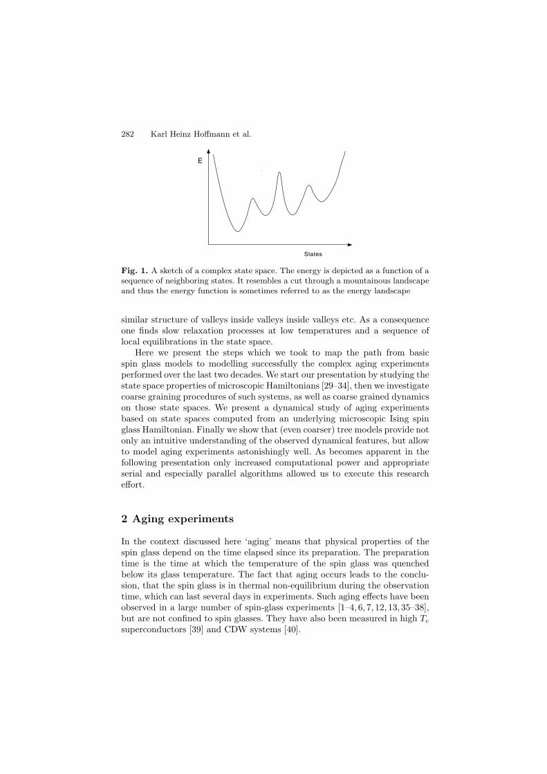
282 Karl Heinz Hoffmann et al.
States
E
Fig. 1. A sketch of a complex state space. The energy is depicted as a function of asequence of neighboring states. It resembles a cut through a mountainous landscapeand thus the energy function is sometimes referred to as the energy landscape
similar structure of valleys inside valleys inside valleys etc. As a consequenceone finds slow relaxation processes at low temperatures and a sequence oflocal equilibrations in the state space.
Here we present the steps which we took to map the path from basicspin glass models to modelling successfully the complex aging experimentsperformed over the last two decades. We start our presentation by studying thestate space properties of microscopic Hamiltonians [29–34], then we investigatecoarse graining procedures of such systems, as well as coarse grained dynamicson those state spaces. We present a dynamical study of aging experimentsbased on state spaces computed from an underlying microscopic Ising spinglass Hamiltonian. Finally we show that (even coarser) tree models provide notonly an intuitive understanding of the observed dynamical features, but allowto model aging experiments astonishingly well. As becomes apparent in thefollowing presentation only increased computational power and appropriateserial and especially parallel algorithms allowed us to execute this researcheffort.
2 Aging experiments
In the context discussed here ‘aging’ means that physical properties of thespin glass depend on the time elapsed since its preparation. The preparationtime is the time at which the temperature of the spin glass was quenchedbelow its glass temperature. The fact that aging occurs leads to the conclu-sion, that the spin glass is in thermal non-equilibrium during the observationtime, which can last several days in experiments. Such aging effects have beenobserved in a large number of spin-glass experiments [1–4, 6, 7, 12, 13, 35–38],but are not confined to spin glasses. They have also been measured in high Tc
superconductors [39] and CDW systems [40].
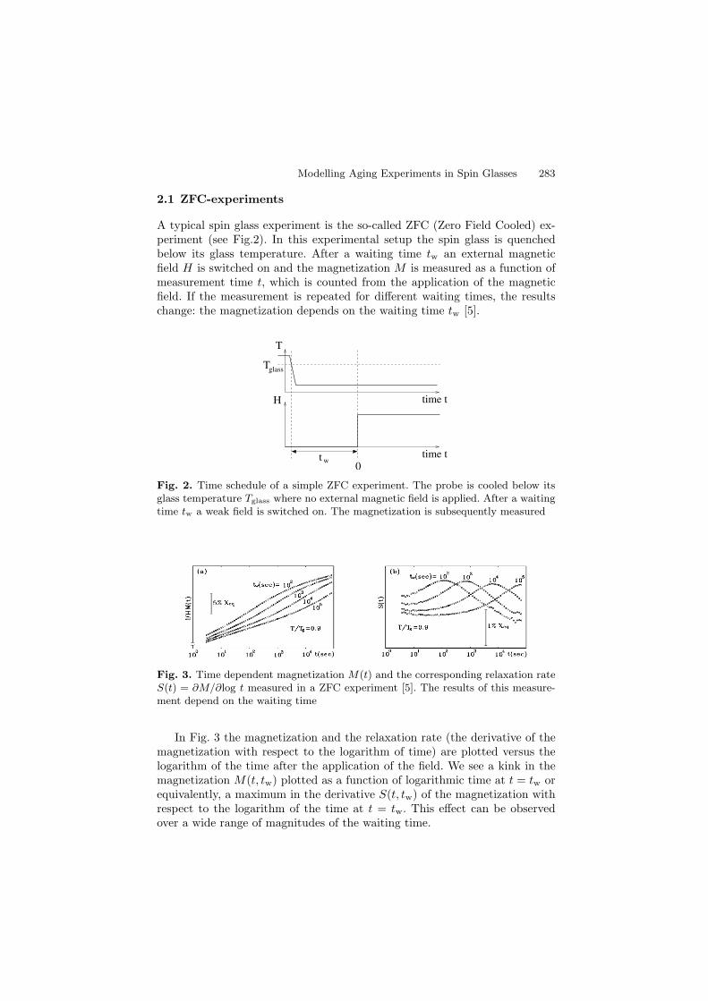
Modelling Aging Experiments in Spin Glasses 283
2.1 ZFC-experiments
A typical spin glass experiment is the so-called ZFC (Zero Field Cooled) ex-periment (see Fig.2). In this experimental setup the spin glass is quenchedbelow its glass temperature. After a waiting time tw an external magneticfield H is switched on and the magnetization M is measured as a function ofmeasurement time t, which is counted from the application of the magneticfield. If the measurement is repeated for different waiting times, the resultschange: the magnetization depends on the waiting time tw [5].
time t
time t
T
Tglass
0t w
H
Fig. 2. Time schedule of a simple ZFC experiment. The probe is cooled below itsglass temperature Tglass where no external magnetic field is applied. After a waitingtime tw a weak field is switched on. The magnetization is subsequently measured
Fig. 3. Time dependent magnetization M(t) and the corresponding relaxation rateS(t) = ∂M/∂log t measured in a ZFC experiment [5]. The results of this measure-ment depend on the waiting time
In Fig. 3 the magnetization and the relaxation rate (the derivative of themagnetization with respect to the logarithm of time) are plotted versus thelogarithm of the time after the application of the field. We see a kink in themagnetization M(t, tw) plotted as a function of logarithmic time at t = tw orequivalently, a maximum in the derivative S(t, tw) of the magnetization withrespect to the logarithm of the time at t = tw. This effect can be observedover a wide range of magnitudes of the waiting time.
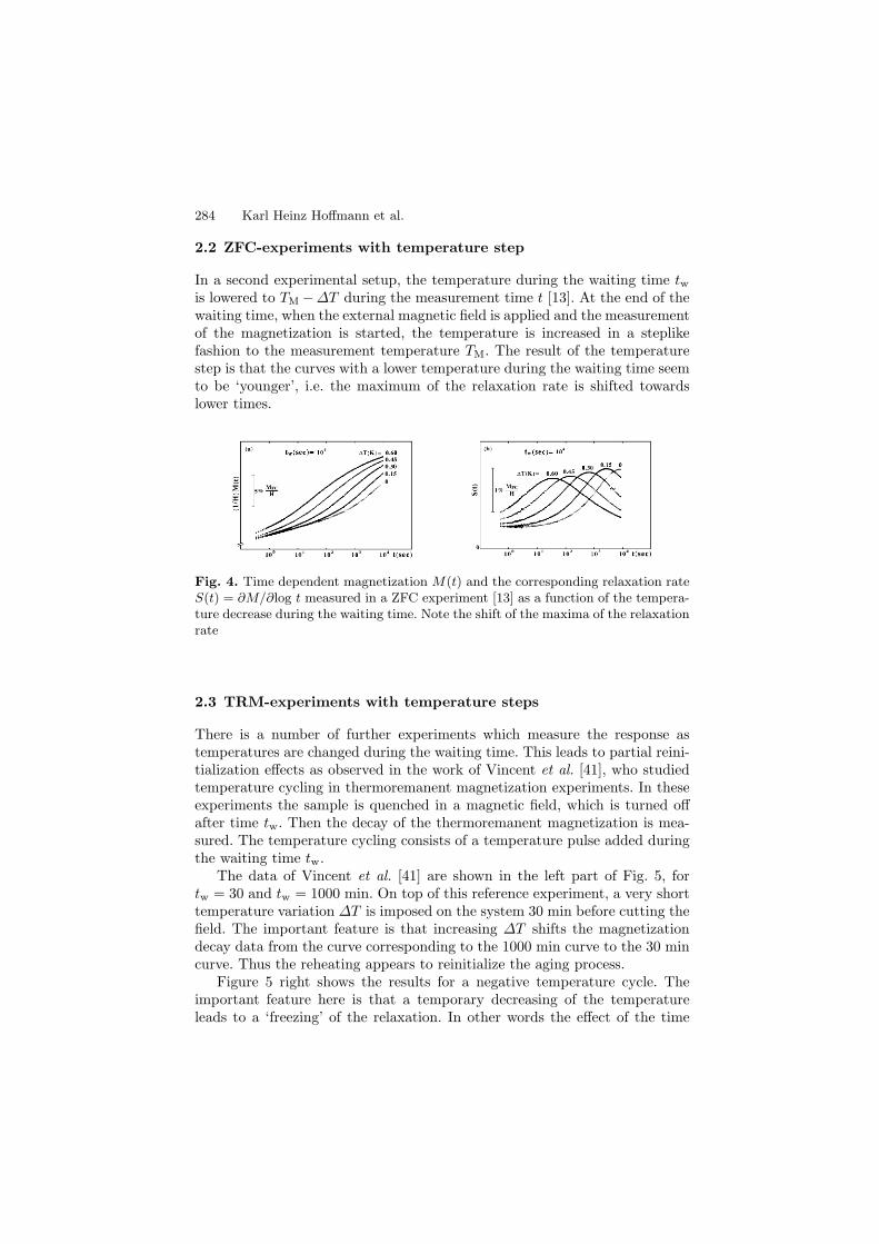
284 Karl Heinz Hoffmann et al.
2.2 ZFC-experiments with temperature step
In a second experimental setup, the temperature during the waiting time twis lowered to TM−∆T during the measurement time t [13]. At the end of thewaiting time, when the external magnetic field is applied and the measurementof the magnetization is started, the temperature is increased in a steplikefashion to the measurement temperature TM. The result of the temperaturestep is that the curves with a lower temperature during the waiting time seemto be ‘younger’, i.e. the maximum of the relaxation rate is shifted towardslower times.
Fig. 4. Time dependent magnetization M(t) and the corresponding relaxation rateS(t) = ∂M/∂log t measured in a ZFC experiment [13] as a function of the tempera-ture decrease during the waiting time. Note the shift of the maxima of the relaxationrate
2.3 TRM-experiments with temperature steps
There is a number of further experiments which measure the response astemperatures are changed during the waiting time. This leads to partial reini-tialization effects as observed in the work of Vincent et al. [41], who studiedtemperature cycling in thermoremanent magnetization experiments. In theseexperiments the sample is quenched in a magnetic field, which is turned offafter time tw. Then the decay of the thermoremanent magnetization is mea-sured. The temperature cycling consists of a temperature pulse added duringthe waiting time tw.
The data of Vincent et al. [41] are shown in the left part of Fig. 5, fortw = 30 and tw = 1000 min. On top of this reference experiment, a very shorttemperature variation ∆T is imposed on the system 30 min before cutting thefield. The important feature is that increasing ∆T shifts the magnetizationdecay data from the curve corresponding to the 1000 min curve to the 30 mincurve. Thus the reheating appears to reinitialize the aging process.
Figure 5 right shows the results for a negative temperature cycle. Theimportant feature here is that a temporary decreasing of the temperatureleads to a ‘freezing’ of the relaxation. In other words the effect of the time
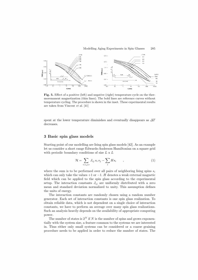
Modelling Aging Experiments in Spin Glasses 285
Fig. 5. Effect of a positive (left) and negative (right) temperature cycle on the ther-moremanent magnetization (thin lines). The bold lines are reference curves withouttemperature cycling. The procedure is shown in the inset. These experimental resultsare taken from Vincent et al. [41]
spent at the lower temperature diminishes and eventually disappears as ∆Tdecreases.
3 Basic spin glass models
Starting point of our modelling are Ising spin glass models [42]. As an examplelet us consider a short range Edwards-Anderson Hamiltonian on a square gridwith periodic boundary conditions of size L x L
H =∑
<i,j>
Jij si sj −∑
i
Hsi , (1)
where the sum is to be performed over all pairs of neighboring Ising spins siwhich can only take the values +1 or −1. H denotes a weak external magneticfield which can be applied to the spin glass according to the experimentalsetup. The interaction constants Jij are uniformly distributed with a zeromean and standard deviation normalized to unity. This assumption definesthe units of energy.
The interaction constants are randomly chosen using a random numbergenerator. Each set of interaction constants is one spin glass realization. Toobtain reliable data, which is not dependent on a single choice of interactionconstants, we have to perform an average over many spin glass realizations.Such an analysis heavily depends on the availability of appropriate computingpower.
The number of states is 2N if N is the number of spins and grows exponen-tially with the system size, a feature common to the systems we are interestedin. Thus either only small systems can be considered or a coarse grainingprocedure needs to be applied in order to reduce the number of states. The
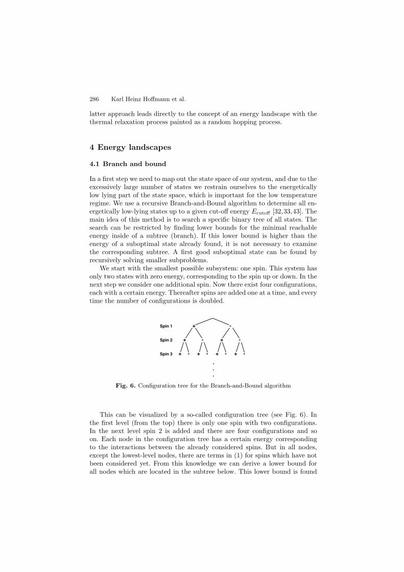
286 Karl Heinz Hoffmann et al.
latter approach leads directly to the concept of an energy landscape with thethermal relaxation process painted as a random hopping process.
4 Energy landscapes
4.1 Branch and bound
In a first step we need to map out the state space of our system, and due to theexcessively large number of states we restrain ourselves to the energeticallylow lying part of the state space, which is important for the low temperatureregime. We use a recursive Branch-and-Bound algorithm to determine all en-ergetically low-lying states up to a given cut-off energy Ecutoff [32,33,43]. Themain idea of this method is to search a specific binary tree of all states. Thesearch can be restricted by finding lower bounds for the minimal reachableenergy inside of a subtree (branch). If this lower bound is higher than theenergy of a suboptimal state already found, it is not necessary to examinethe corresponding subtree. A first good suboptimal state can be found byrecursively solving smaller subproblems.
We start with the smallest possible subsystem: one spin. This system hasonly two states with zero energy, corresponding to the spin up or down. In thenext step we consider one additional spin. Now there exist four configurations,each with a certain energy. Thereafter spins are added one at a time, and everytime the number of configurations is doubled.
+
+ -
+
+ -
+
-
+
.
-
Spin 1
Spin 2
Spin 3
-
-
+ -
.
.
Fig. 6. Configuration tree for the Branch-and-Bound algorithm
This can be visualized by a so-called configuration tree (see Fig. 6). Inthe first level (from the top) there is only one spin with two configurations.In the next level spin 2 is added and there are four configurations and soon. Each node in the configuration tree has a certain energy correspondingto the interactions between the already considered spins. But in all nodes,except the lowest-level nodes, there are terms in (1) for spins which have notbeen considered yet. From this knowledge we can derive a lower bound forall nodes which are located in the subtree below. This lower bound is found
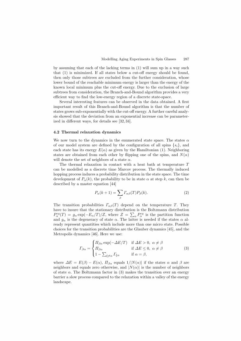
Modelling Aging Experiments in Spin Glasses 287
by assuming that each of the lacking terms in (1) will sum up in a way suchthat (1) is minimized. If all states below a cut-off energy should be found,then only those subtrees are excluded from the further consideration, whoselower bound of the reachable minimum energy is larger than the energy of theknown local minimum plus the cut-off energy. Due to the exclusion of largesubtrees from consideration, the Branch-and-Bound algorithm provides a veryefficient way to find the low-energy region of a discrete state-space.
Several interesting features can be observed in the data obtained. A firstimportant result of this Branch-and-Bound algorithm is that the number ofstates grows sub-exponentially with the cut-off energy. A further careful analy-sis showed that the deviation from an exponential increase can be parameter-ized in different ways, for details see [32,34].
4.2 Thermal relaxation dynamics
We now turn to the dynamics in the enumerated state space. The states αof our model system are defined by the configuration of all spins si, andeach state has its energy E(α) as given by the Hamiltonian (1). Neighboringstates are obtained from each other by flipping one of the spins, and N(α)will denote the set of neighbors of a state α.
The thermal relaxation in contact with a heat bath at temperature Tcan be modelled as a discrete time Marcov process. The thermally inducedhopping process induces a probability distribution in the state space. The timedevelopment of Pα(k), the probability to be in state α at step k, can then bedescribed by a master equation [44]
Pα(k + 1) =∑
β
Γαβ(T )Pβ(k). (2)
The transition probabilities Γαβ(T ) depend on the temperature T . Theyhave to insure that the stationary distribution is the Boltzmann distributionP eq
α (T ) = gα exp(−Eα/T )/Z, where Z =∑
α Peqα is the partition function
and gα is the degeneracy of state α. The latter is needed if the states α al-ready represent quantities which include more than one micro state. Possiblechoices for the transition probabilities are the Glauber dynamics [45], and theMetropolis dynamics [46]. Here we use:
Γβα =
Πβα exp(−∆E/T ) if ∆E > 0, α = βΠβα if ∆E ≤ 0, α = β1−∑
ξ =α Γξα if α = β,
(3)
where ∆E = E(β) − E(α), Πβα equals 1/|N(α)| if the states α and β areneighbors and equals zero otherwise, and |N(α)| is the number of neighborsof state α. The Boltzmann factor in (3) makes the transition over an energybarrier a slow process compared to the relaxation within a valley of the energylandscape.
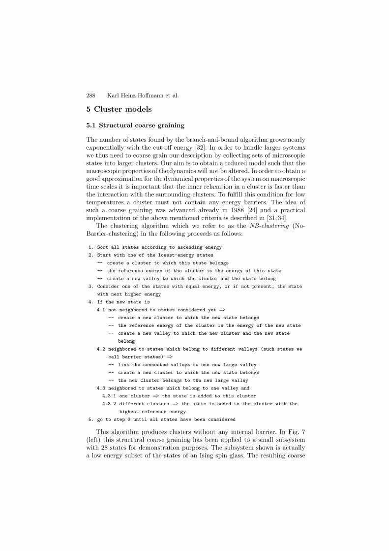
288 Karl Heinz Hoffmann et al.
5 Cluster models
5.1 Structural coarse graining
The number of states found by the branch-and-bound algorithm grows nearlyexponentially with the cut-off energy [32]. In order to handle larger systemswe thus need to coarse grain our description by collecting sets of microscopicstates into larger clusters. Our aim is to obtain a reduced model such that themacroscopic properties of the dynamics will not be altered. In order to obtain agood approximation for the dynamical properties of the system on macroscopictime scales it is important that the inner relaxation in a cluster is faster thanthe interaction with the surrounding clusters. To fulfill this condition for lowtemperatures a cluster must not contain any energy barriers. The idea ofsuch a coarse graining was advanced already in 1988 [24] and a practicalimplementation of the above mentioned criteria is described in [31,34].
The clustering algorithm which we refer to as the NB-clustering (No-Barrier-clustering) in the following proceeds as follows:
1. Sort all states according to ascending energy
2. Start with one of the lowest-energy states
-- create a cluster to which this state belongs
-- the reference energy of the cluster is the energy of this state
-- create a new valley to which the cluster and the state belong
3. Consider one of the states with equal energy, or if not present, the state
with next higher energy
4. If the new state is
4.1 not neighbored to states considered yet ⇒-- create a new cluster to which the new state belongs
-- the reference energy of the cluster is the energy of the new state
-- create a new valley to which the new cluster and the new state
belong
4.2 neighbored to states which belong to different valleys (such states we
call barrier states) ⇒-- link the connected valleys to one new large valley
-- create a new cluster to which the new state belongs
-- the new cluster belongs to the new large valley
4.3 neighbored to states which belong to one valley and
4.3.1 one cluster ⇒ the state is added to this cluster
4.3.2 different clusters ⇒ the state is added to the cluster with the
highest reference energy
5. go to step 3 until all states have been considered
This algorithm produces clusters without any internal barrier. In Fig. 7(left) this structural coarse graining has been applied to a small subsystemwith 28 states for demonstration purposes. The subsystem shown is actuallya low energy subset of the states of an Ising spin glass. The resulting coarse
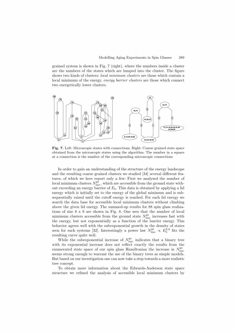
Modelling Aging Experiments in Spin Glasses 289
grained system is shown in Fig. 7 (right), where the numbers inside a clusterare the numbers of the states which are lumped into the cluster. The figureshows two kinds of clusters: local minimum clusters are those which contain alocal minimum of the energy, energy barrier clusters are those which connecttwo energetically lower clusters.
96
46
78
58
8
10
70
48
36
22
54
34
28
2420
14
12
32
30
52
64
6668
72
84
4
6
18
8,10,58,78,96
2
52,72
4,6,22,36,84
12,14,18,20,30,32,46
64,66,68
24,28,34
54
48,70
2 2
2
4
1
Fig. 7. Left: Microscopic states with connections. Right: Coarse grained state spaceobtained from the microscopic states using the algorithm. The number in a squareat a connection is the number of the corresponding microscopic connections
In order to gain an understanding of the structure of the energy landscapeand the resulting coarse grained clusters we studied [34] several different fea-tures, of which we here report only a few: First we analysed the number oflocal minimum clusters Ngs
lmc, which are accessible from the ground state with-out exceeding an energy barrier of Eb. This data is obtained by applying a lidenergy which is initially set to the energy of the global minimum and is sub-sequentially raised until the cutoff energy is reached. For each lid energy wesearch the data base for accessible local minimum clusters without climbingabove the given lid energy. The summed-up results for 88 spin glass realiza-tions of size 8 x 8 are shown in Fig. 8. One sees that the number of localminimum clusters accessible from the ground state Ngs
lmc increases fast withthe energy, but not exponentially as a function of the barrier energy. Thisbehavior agrees well with the subexponential growth in the density of statesseen for such systems [32]. Interestingly a power law Ngs
lmc ∝ E3.9b fits the
resulting curve quite well.While the subexponential increase of Ngs
lmc indicates that a binary treewith its exponential increase does not reflect exactly the results from theenumerated state space of our spin glass Hamiltonian the increase in Ngs
lmc
seems strong enough to warrant the use of the binary trees as simple models.But based on our investigation one can now take a step towards a more realistictree concept.
To obtain more information about the Edwards-Anderson state spacestructure we refined the analysis of accessible local minimum clusters by
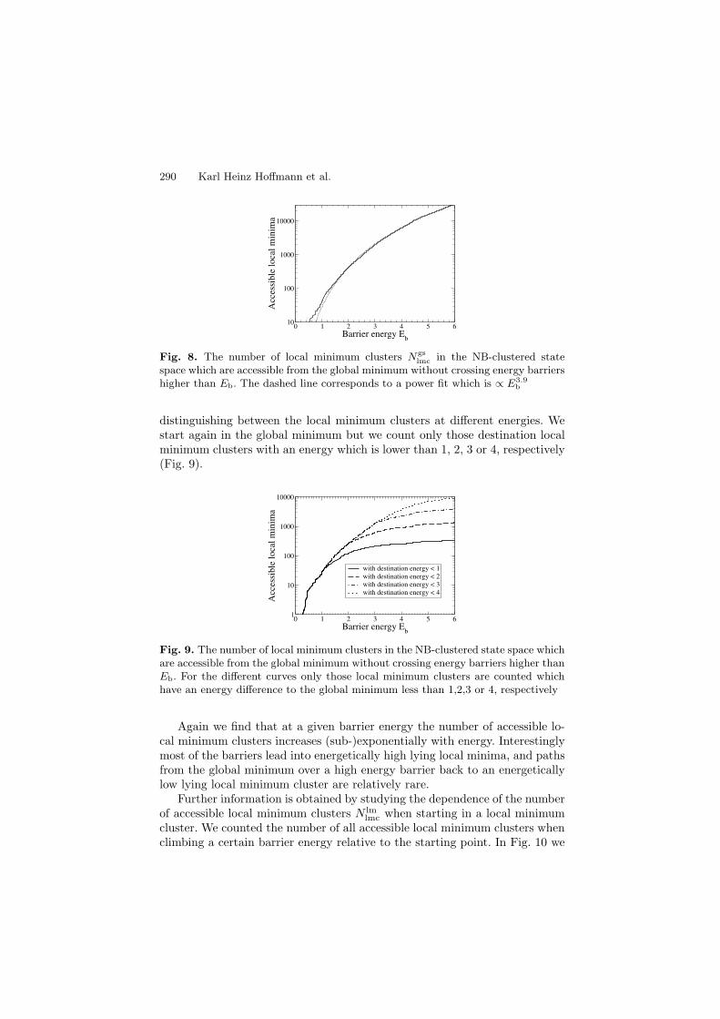
290 Karl Heinz Hoffmann et al.
0 1 2 3 4 5 6Barrier energy E
b
10
100
1000
10000
Acc
essi
ble
loca
l m
inim
a
Fig. 8. The number of local minimum clusters Ngslmc in the NB-clustered state
space which are accessible from the global minimum without crossing energy barriershigher than Eb. The dashed line corresponds to a power fit which is ∝ E3.9
b
distinguishing between the local minimum clusters at different energies. Westart again in the global minimum but we count only those destination localminimum clusters with an energy which is lower than 1, 2, 3 or 4, respectively(Fig. 9).
0 1 2 3 4 5 6Barrier energy E
b
1
10
100
1000
10000
Acc
essi
ble
loca
l m
inim
a
with destination energy < 1with destination energy < 2with destination energy < 3with destination energy < 4
Fig. 9. The number of local minimum clusters in the NB-clustered state space whichare accessible from the global minimum without crossing energy barriers higher thanEb. For the different curves only those local minimum clusters are counted whichhave an energy difference to the global minimum less than 1,2,3 or 4, respectively
Again we find that at a given barrier energy the number of accessible lo-cal minimum clusters increases (sub-)exponentially with energy. Interestinglymost of the barriers lead into energetically high lying local minima, and pathsfrom the global minimum over a high energy barrier back to an energeticallylow lying local minimum cluster are relatively rare.
Further information is obtained by studying the dependence of the numberof accessible local minimum clusters N lm
lmc when starting in a local minimumcluster. We counted the number of all accessible local minimum clusters whenclimbing a certain barrier energy relative to the starting point. In Fig. 10 we
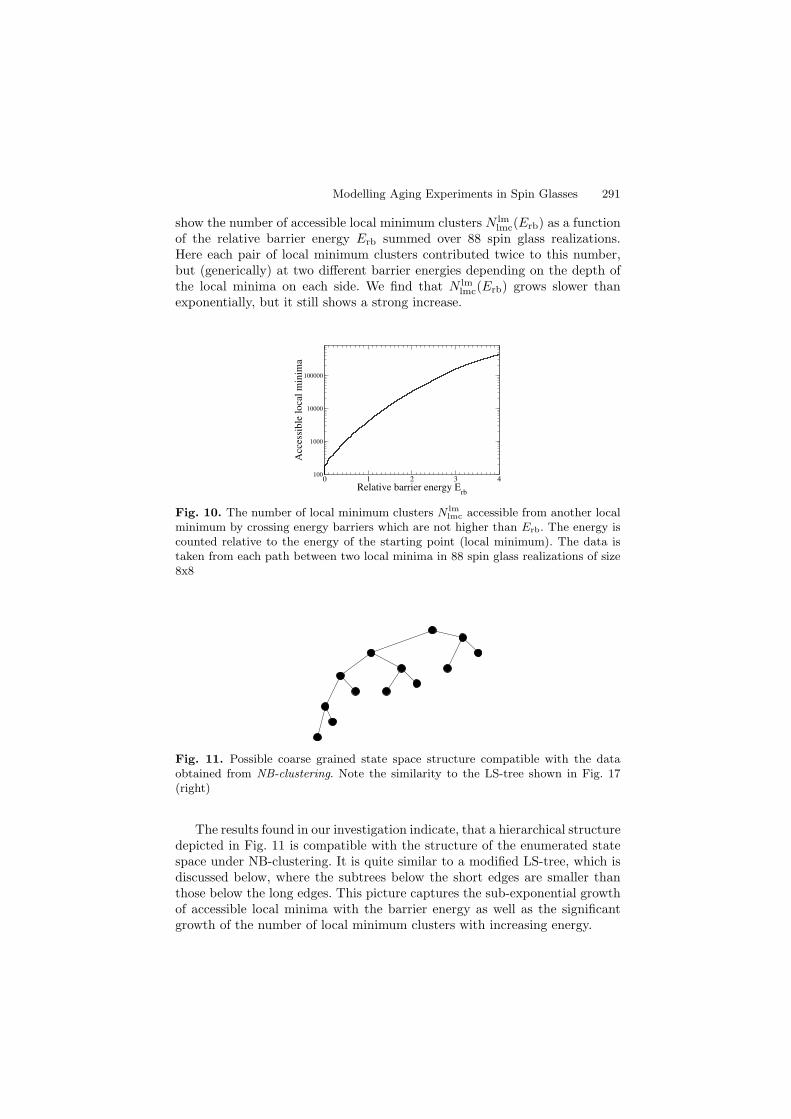
Modelling Aging Experiments in Spin Glasses 291
show the number of accessible local minimum clusters N lmlmc(Erb) as a function
of the relative barrier energy Erb summed over 88 spin glass realizations.Here each pair of local minimum clusters contributed twice to this number,but (generically) at two different barrier energies depending on the depth ofthe local minima on each side. We find that N lm
lmc(Erb) grows slower thanexponentially, but it still shows a strong increase.
0 1 2 3 4Relative barrier energy E
rb
100
1000
10000
100000
Acc
essi
ble
loca
l m
inim
a
Fig. 10. The number of local minimum clusters N lmlmc accessible from another local
minimum by crossing energy barriers which are not higher than Erb. The energy iscounted relative to the energy of the starting point (local minimum). The data istaken from each path between two local minima in 88 spin glass realizations of size8x8
Fig. 11. Possible coarse grained state space structure compatible with the dataobtained from NB-clustering. Note the similarity to the LS-tree shown in Fig. 17(right)
The results found in our investigation indicate, that a hierarchical structuredepicted in Fig. 11 is compatible with the structure of the enumerated statespace under NB-clustering. It is quite similar to a modified LS-tree, which isdiscussed below, where the subtrees below the short edges are smaller thanthose below the long edges. This picture captures the sub-exponential growthof accessible local minima with the barrier energy as well as the significantgrowth of the number of local minimum clusters with increasing energy.

292 Karl Heinz Hoffmann et al.
5.2 Dynamical coarse graining
Consider now the thermal hopping on the complex energy landscape. Ratherthan calculating the full time dependence of the probability distribution inthe enumerated state space, we can choose to monitor the presence or ab-sence from a cluster of the coarse grained system. We have hereby defined astochastic process, which in general will not be a Marcov process [47], becausethe induced transition probability from cluster to cluster might depend on theinternal (microscopic) distribution within one cluster. However, it turns outthat inside a coarse grained area very quickly a kind of local equilibrium distri-bution is established, which then makes the coarse grained relaxation process(at least approximately) marcovian. The result is that Marcov processes onthe coarse grained systems are good modelling tools for the thermal relaxationof complex systems [23,24,48].
Using this insight, the proper transition rates of the coarse grained systemcan be determined. To find the structure of this rates let us start with theexact calculation of the transition probability between two neighboring clus-ters based on the microscopic picture. The probability flux from the statesbelonging to cluster Cν to the states belonging to cluster Cµ is given by
Jµν = GµνPν =∑
α∈Cµ,β∈Cν
Γαβpβ , (4)
where Pν is the total probability to be in cluster Cν , i.e. the sum of theprobabilities of all states in cluster Cν , and Gµν is the transition rate fromcluster Cν to cluster Cµ. Again we assume that the internal relaxation in-side the clusters is fast compared to the relaxation between different clus-ters. For the time scale of interest all clusters are in internal equilibrium,i.e. pβ ∝ exp(−Eβ/T ). As the microscopic transition rates have the formΓαβ ∝ exp(−max(Eα − Eβ , 0)/T ), the coarse grained transition rate is
Gµν =
∑α∈Cµ,β∈Cν
Παβexp(−max(Eα, Eβ)/T )∑
α∈Cνexp(−Eα/T )
. (5)
The roughest simplification (here referred to as procedure A) would be toconsider all states of a cluster as one state with a certain energy Eµ which ischosen as the mean energy of the microscopic states. Following this idea thesums in (5) can be simplified to
Gµν =Tµνmin(exp(−(Eµ − Eν)/T ), 1)
nν, (6)
where Tµν is related to the number of connections between cluster Cν andcluster Cµ, and nν is the number of states collected in cluster Cν . A betterapproximation can be achieved if each cluster is modelled by a two-level sys-tem, which is in internal equilibrium (procedure B). For a detailed descriptionof these procedures see Klotz et al. [31].
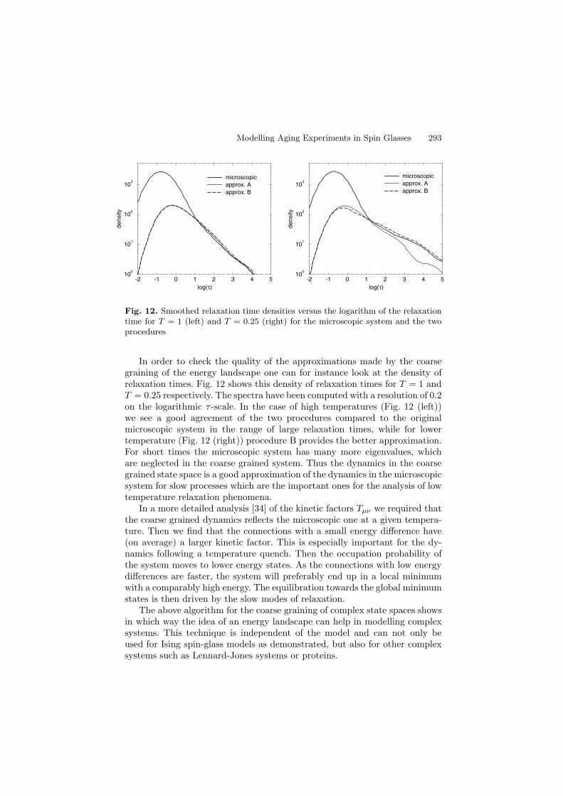
Modelling Aging Experiments in Spin Glasses 293
-2 -1 0 1 2 3 4 5
log(τ)
100
101
102
103
de
nsi
ty
microscopic
approx. Aapprox. B
-2 -1 0 1 2 3 4 5
log(τ)
100
101
102
103
de
nsi
ty
microscopicapprox. A
approx. B
Fig. 12. Smoothed relaxation time densities versus the logarithm of the relaxationtime for T = 1 (left) and T = 0.25 (right) for the microscopic system and the twoprocedures
In order to check the quality of the approximations made by the coarsegraining of the energy landscape one can for instance look at the density ofrelaxation times. Fig. 12 shows this density of relaxation times for T = 1 andT = 0.25 respectively. The spectra have been computed with a resolution of 0.2on the logarithmic τ -scale. In the case of high temperatures (Fig. 12 (left))we see a good agreement of the two procedures compared to the originalmicroscopic system in the range of large relaxation times, while for lowertemperature (Fig. 12 (right)) procedure B provides the better approximation.For short times the microscopic system has many more eigenvalues, whichare neglected in the coarse grained system. Thus the dynamics in the coarsegrained state space is a good approximation of the dynamics in the microscopicsystem for slow processes which are the important ones for the analysis of lowtemperature relaxation phenomena.
In a more detailed analysis [34] of the kinetic factors Tµν we required thatthe coarse grained dynamics reflects the microscopic one at a given tempera-ture. Then we find that the connections with a small energy difference have(on average) a larger kinetic factor. This is especially important for the dy-namics following a temperature quench. Then the occupation probability ofthe system moves to lower energy states. As the connections with low energydifferences are faster, the system will preferably end up in a local minimumwith a comparably high energy. The equilibration towards the global minimumstates is then driven by the slow modes of relaxation.
The above algorithm for the coarse graining of complex state spaces showsin which way the idea of an energy landscape can help in modelling complexsystems. This technique is independent of the model and can not only beused for Ising spin-glass models as demonstrated, but also for other complexsystems such as Lennard-Jones systems or proteins.
294 Karl Heinz Hoffmann et al.
6 Aging in the enumerated state space
We now turn to the modelling of the aging experiments. If the concepts pre-sented above are valid, then one should be able to simulate the aging behaviorbased on the coarse grained dynamics. First we investigate a simple ZFC ex-periment where the spin glass is quenched below its glass temperature with noexternal magnetic field. We perform the analysis on the low-energy part of anenumerated and coarse grained state space derived from our spin glass Hamil-tonian. In this approach we directly access the properties of the state space(e.g., the energy and magnetization of the clusters) and perform a dynamicsfollowing the Metropolis algorithm.
To model experiments with an external magnetic field we set H = 0 inthe second term of the Hamiltonian (1). While in principle the external fieldchanges the state space structure and the coarse graining procedure shouldbe redone for the state space in the external field, we here assume that themagnetic field is weak and that it changes only slightly the structure of thestate space. Thus we just change the energies of the already coarse grainedsystem
EHµ = Eµ −HMµ , (7)
for all Clusters p. Mµ is the effective magnetization of the cluster Cµ, whichis computed from the magnetizations of the micro-states in this cluster andthe assumption of internal equilibration at the given temperature, and
Eµ = −T ln
1
nµ
∑
α∈Cµ
e−Eα/T
. (8)
Technically we solve the eigenvalue problem of the corresponding masterequation determining eigenvalues and eigenvectors. Then macroscopic proper-ties of the spin glass can be obtained by performing the thermal average andthe average over many spin glass realizations (ensemble average). We simu-lated the ZFC procedure in 500 spin glass realizations with altogether morethan 17 million micro-states. They can be reduced to coarse grained statespaces with about 276.000 clusters. Our choice for the external magnetic fieldwas H = 0.1 and for the temperature T = 0.2.
The averaged results of these calculations are shown in Fig. 13. The mag-netization increases after the application of the magnetic field, since the spinstend to align with the direction of the external field. States with positive mag-netization become energetically favored. However, we find that the magneti-zation increases slower in the curves with a larger waiting time. This systemclearly shows aging features. The corresponding curves of the relaxation rateS(t) = dM(t)/d log(t) in Fig. 14 display maxima at times which are roughlyequal to the waiting time.
This remarkable result indicates that the considered coarse grained statespace still represents all ingredients necessary for aging effects. We find that
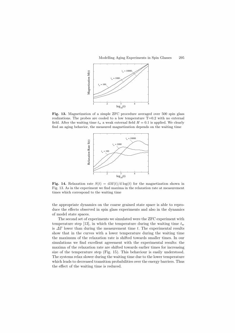
Modelling Aging Experiments in Spin Glasses 295
1 2 3 4 5log
10(t)
Mag
neti
zati
on M
(t)
tw
= 100
tw
= 1000
tw
= 10000
Fig. 13. Magnetization of a simple ZFC procedure averaged over 500 spin glassrealizations. The probes are cooled to a low temperature T=0.2 with no externalfield. After the waiting time tw a weak external field H = 0.1 is applied. We clearlyfind an aging behavior, the measured magnetization depends on the waiting time
1 2 3 4 5log
10(t)
Rel
axat
ion
Rat
e S
(t)
tw
= 10000
tw
= 1000
tw
= 100
Fig. 14. Relaxation rate S(t) = dM(t)/d log(t) for the magnetization shown inFig. 13. As in the experiment we find maxima in the relaxation rate at measurementtimes which correspond to the waiting time
the appropriate dynamics on the coarse grained state space is able to repro-duce the effects observed in spin glass experiments and also in the dynamicsof model state spaces.
The second set of experiments we simulated were the ZFC experiment withtemperature step [13], in which the temperature during the waiting time twis ∆T lower than during the measurement time t. The experimental resultsshow that in the curves with a lower temperature during the waiting timethe maximum of the relaxation rate is shifted towards smaller times. In oursimulations we find excellent agreement with the experimental results: themaxima of the relaxation rate are shifted towards earlier times for increasingsize of the temperature step (Fig. 15). This behaviour is easily understood.The systems relax slower during the waiting time due to the lower temperaturewhich leads to decreased transition probabilities over the energy barriers. Thusthe effect of the waiting time is reduced.
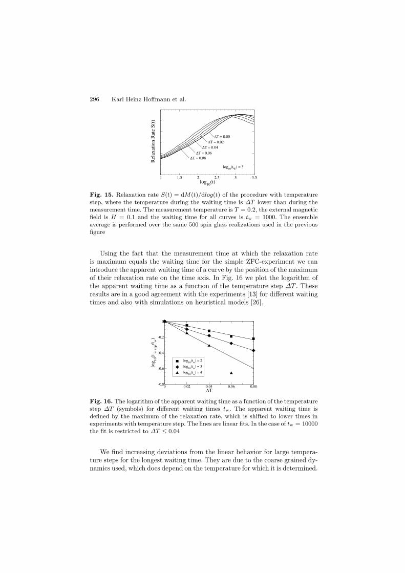
296 Karl Heinz Hoffmann et al.
1 1.5 2 2.5 3 3.5log
10(t)
Rel
axat
ion
Rat
e S
(t)
∆Τ = 0.00
∆Τ = 0.04
∆Τ = 0.06∆Τ = 0.08
∆Τ = 0.02
log10
(tW
) = 3
Fig. 15. Relaxation rate S(t) = dM(t)/dlog(t) of the procedure with temperaturestep, where the temperature during the waiting time is ∆T lower than during themeasurement time. The measurement temperature is T = 0.2, the external magneticfield is H = 0.1 and the waiting time for all curves is tw = 1000. The ensembleaverage is performed over the same 500 spin glass realizations used in the previousfigure
Using the fact that the measurement time at which the relaxation rateis maximum equals the waiting time for the simple ZFC-experiment we canintroduce the apparent waiting time of a curve by the position of the maximumof their relaxation rate on the time axis. In Fig. 16 we plot the logarithm ofthe apparent waiting time as a function of the temperature step ∆T . Theseresults are in a good agreement with the experiments [13] for different waitingtimes and also with simulations on heuristical models [26].
0 0.02 0.04 0.06 0.08∆Τ
-0.8
-0.6
-0.4
-0.2
0
log
10(t
w a
pp/t
w)
log10
(tw
) = 2
log10
(tw
) = 3
log10
(tw
) = 4
Fig. 16. The logarithm of the apparent waiting time as a function of the temperaturestep ∆T (symbols) for different waiting times tw. The apparent waiting time isdefined by the maximum of the relaxation rate, which is shifted to lower times inexperiments with temperature step. The lines are linear fits. In the case of tw = 10000the fit is restricted to ∆T ≤ 0.04
We find increasing deviations from the linear behavior for large tempera-ture steps for the longest waiting time. They are due to the coarse grained dy-namics used, which does depend on the temperature for which it is determined.
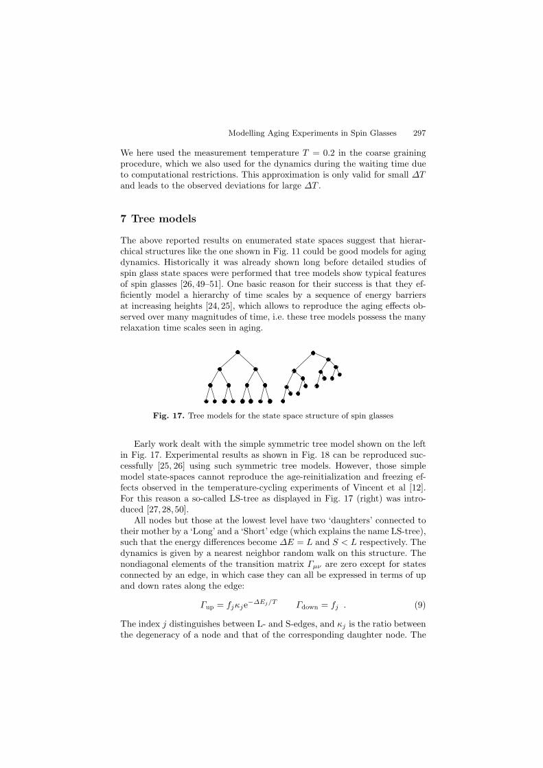
Modelling Aging Experiments in Spin Glasses 297
We here used the measurement temperature T = 0.2 in the coarse grainingprocedure, which we also used for the dynamics during the waiting time dueto computational restrictions. This approximation is only valid for small ∆Tand leads to the observed deviations for large ∆T .
7 Tree models
The above reported results on enumerated state spaces suggest that hierar-chical structures like the one shown in Fig. 11 could be good models for agingdynamics. Historically it was already shown long before detailed studies ofspin glass state spaces were performed that tree models show typical featuresof spin glasses [26, 49–51]. One basic reason for their success is that they ef-ficiently model a hierarchy of time scales by a sequence of energy barriersat increasing heights [24, 25], which allows to reproduce the aging effects ob-served over many magnitudes of time, i.e. these tree models possess the manyrelaxation time scales seen in aging.
Fig. 17. Tree models for the state space structure of spin glasses
Early work dealt with the simple symmetric tree model shown on the leftin Fig. 17. Experimental results as shown in Fig. 18 can be reproduced suc-cessfully [25, 26] using such symmetric tree models. However, those simplemodel state-spaces cannot reproduce the age-reinitialization and freezing ef-fects observed in the temperature-cycling experiments of Vincent et al [12].For this reason a so-called LS-tree as displayed in Fig. 17 (right) was intro-duced [27,28,50].
All nodes but those at the lowest level have two ‘daughters’ connected totheir mother by a ‘Long’ and a ‘Short’ edge (which explains the name LS-tree),such that the energy differences become ∆E = L and S < L respectively. Thedynamics is given by a nearest neighbor random walk on this structure. Thenondiagonal elements of the transition matrix Γµν are zero except for statesconnected by an edge, in which case they can all be expressed in terms of upand down rates along the edge:
Γup = fjκje−∆Ej/T Γdown = fj . (9)
The index j distinguishes between L- and S-edges, and κj is the ratio betweenthe degeneracy of a node and that of the corresponding daughter node. The
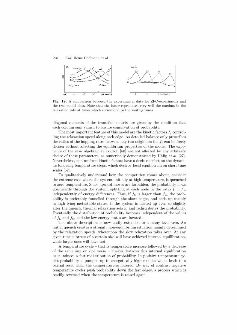
298 Karl Heinz Hoffmann et al.
S(t
) (a
.u.)
log(t) (a.u.)
log(t )= W
2.0 3.04.0
5.0
2 3 4 5
Fig. 18. A comparison between the experimental data for ZFC-experiments andthe tree model data. Note that the latter reproduces very well the maxima in therelaxation rate at times which correspond to the waiting times
diagonal elements of the transition matrix are given by the condition thateach column sum vanish to ensure conservation of probability.
The most important feature of this model are the kinetic factors fj control-ling the relaxation speed along each edge. As detailed balance only prescribesthe ratios of the hopping rates between any two neighbors the fj can be freelychosen without affecting the equilibrium properties of the model. The expo-nents of the slow algebraic relaxation [50] are not affected by any arbitrarychoice of these parameters, as numerically demonstrated by Uhlig et al. [27].Nevertheless, non-uniform kinetic factors have a decisive effect on the dynam-ics following temperature steps, which destroy local equilibrium on short timescales [52].
To qualitatively understand how the competition comes about, considerthe extreme case where the system, initially at high temperature, is quenchedto zero temperature. Since upward moves are forbidden, the probability flowsdownwards through the system, splitting at each node in the ratio fL : fS,independently of energy differences. Thus, if fS is larger than fL, the prob-ability is preferably funnelled through the short edges, and ends up mainlyin high lying metastable states. If the system is heated up even so slightlyafter the quench, thermal relaxation sets in and redistributes the probability.Eventually the distribution of probability becomes independent of the valuesof fL and fS, and the low energy states are favored.
The above description is now easily extended to a many level tree. Aninitial quench creates a strongly non-equilibrium situation mainly determinedby the relaxation speeds, whereupon the slow relaxation takes over. At anygiven time subtrees of a certain size will have achieved internal equilibration,while larger ones will have not.
A temperature cycle – that is temperature increase followed by a decreaseof the same size or vice versa – always destroys this internal equilibrationas it induces a fast redistribution of probability. In positive temperature cy-cles probability is pumped up to energetically higher nodes which leads to apartial reset when the temperature is lowered. By way of contrast negativetemperature cycles push probability down the fast edges, a process which isreadily reversed when the temperature is raised again.
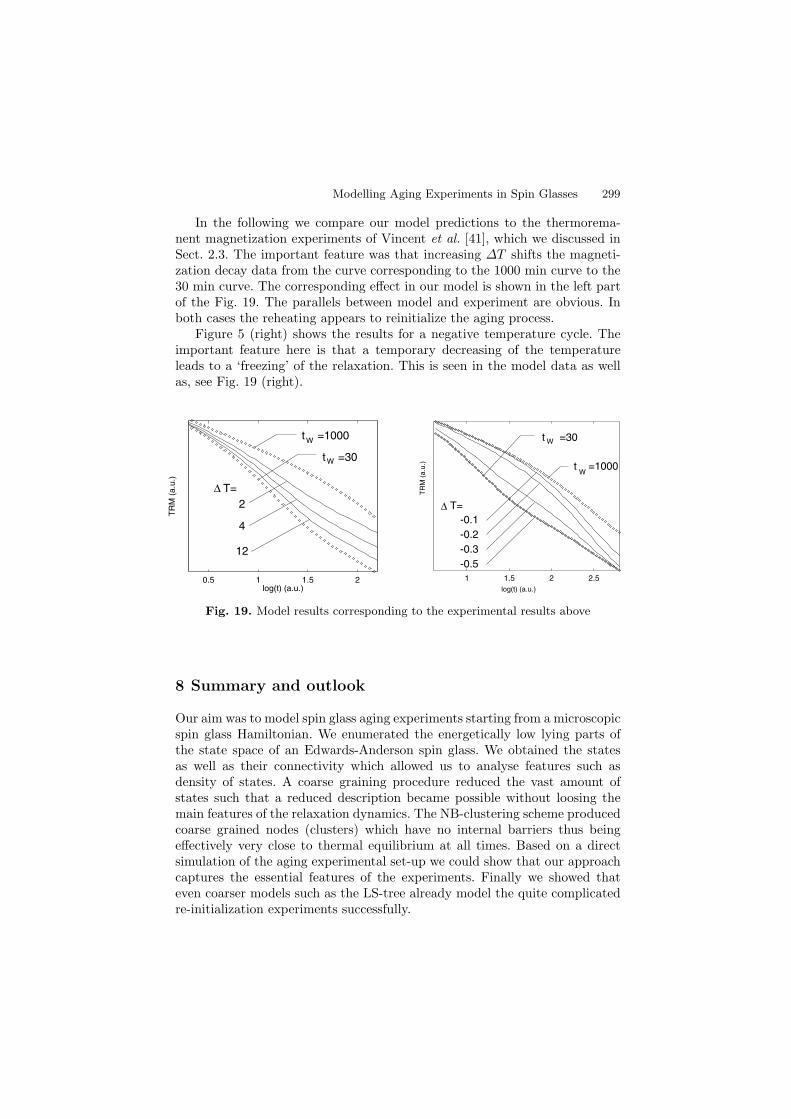
Modelling Aging Experiments in Spin Glasses 299
In the following we compare our model predictions to the thermorema-nent magnetization experiments of Vincent et al. [41], which we discussed inSect. 2.3. The important feature was that increasing ∆T shifts the magneti-zation decay data from the curve corresponding to the 1000 min curve to the30 min curve. The corresponding effect in our model is shown in the left partof the Fig. 19. The parallels between model and experiment are obvious. Inboth cases the reheating appears to reinitialize the aging process.
Figure 5 (right) shows the results for a negative temperature cycle. Theimportant feature here is that a temporary decreasing of the temperatureleads to a ‘freezing’ of the relaxation. This is seen in the model data as wellas, see Fig. 19 (right).
W
0.5 1 1.5 2
TR
M (
a.u
.)
log(t) (a.u.)
Wt =1000
2
4
12
T=∆
t =30
-0.5
-0.3
1 1.5 2 2.5
-0.2
TR
M (
a.u
.)
-0.1
T=∆
W
W
t =30
t =1000
log(t) (a.u.)
Fig. 19. Model results corresponding to the experimental results above
8 Summary and outlook
Our aim was to model spin glass aging experiments starting from a microscopicspin glass Hamiltonian. We enumerated the energetically low lying parts ofthe state space of an Edwards-Anderson spin glass. We obtained the statesas well as their connectivity which allowed us to analyse features such asdensity of states. A coarse graining procedure reduced the vast amount ofstates such that a reduced description became possible without loosing themain features of the relaxation dynamics. The NB-clustering scheme producedcoarse grained nodes (clusters) which have no internal barriers thus beingeffectively very close to thermal equilibrium at all times. Based on a directsimulation of the aging experimental set-up we could show that our approachcaptures the essential features of the experiments. Finally we showed thateven coarser models such as the LS-tree already model the quite complicatedre-initialization experiments successfully.
300 Karl Heinz Hoffmann et al.
This research program was only possible because we could make use of thecompute power available to us. This rested partly on the the hardware in formof parallel machines as well as compute clusters but to an even larger extenton the efficient algorithms and their implementation we developed over theyears.
Acknowledgements
KHH thanks Paolo Sibani for numerous discussions about aging experimentsand their modelling and our continued collaboration over the last two decades.
References
1. L. Lundgren, P. Svedlindh, P. Nordblad, and P. Beckman. Dynamics of therelaxation-time spectrum in a cumn spin-glass. Phys. Rev. Lett., 51(10):911–914, 1983.
2. M. Ocio, H. Bouchiat, and P. Monod. Observation of 1/f magnetic fluctuationsin a spin glass. J. Phys. Lett. France, 46:647–652, 1985.
3. P. Nordblad, P. Svedlindh, J. Ferre, and M. Ayadi. Cd0.6Mn0.4Te, a semicon-ducting spin glass. Journal of Magnetism and Magnetic Materials, 59(3–4):250–254, 1986.
4. Ph. Refregier, M. Ocio, J. Hammann, and E. Vincent. Nonstationary spinglass dynamics from susceptibility and noise measurements. J. Appl. Phys.,63(8):4343–4345, 1988.
5. P. Svedlindh, P. Granberg, P. Nordblad, L. Lundgren, and H. S. Chen. Re-laxation in spin glasses at weak magnetic fields. Phys. Rev. B, 35(1):268–273,1987.
6. J. Hamman, M. Lederman, M. Ocio, R. Orbach, and E. Vincent. Spin-glassdynamics – relation between theory and experiment – a beginning. Physica A,185(1–4):278–294, 1992.
7. A. G. Schins, E. M. Dons, A. F. M. Arts, H. W. de Wijn, E. Vincent,L. Leylekian, and J. Hammann. Aging in two-dimensional ising spin glasses.Phys. Rev. B, 48(22):16524–16532, 1993.
8. C. Djurberg, K. Jonason, and P. Nordblad. Magnetic relaxation phenomena ina CuMn spin glass. Eur. Phys. J. B, 10(1):15–21, 1999.
9. K. Jonason, P. Nordblad, E. Vincent, J. Hammann, and J.-P. Bouchaud. Mem-ory interference effects in spin glasses. Eur. Phys. J. B, 13(1):99–105, 2000.
10. R. Mathieu, P. Jonsson, D. N. H. Nam, and P. Nordblad. Memory and super-position in a spin glass. Phys. Rev. B, 63(09):092401/1–092401/4, 2001.
11. R. Mathieu, P. E. Jonsson, P. Nordblad, H. Aruga Katori, and A. Ito. Memoryand chaos in an ising spin glass. Phys. Rev. B, 65(1):012411/1–012411/4, 2002.
12. E. Vincent, J. Hammann, and M. Ocio. Slow dynamics in spin glasses and othercomplex systems. In D. H. Ryan, editor, Recent Progress in Random Magnets,page 207. World Scientific, Singapore, 1992.
13. P. Granberg, L. Sandlund, P. Norblad, P. Svedlindh, and L. Lundgren. Obser-vation of a time-dependent spatial correlation length in a metallic spin glass.Phys. Rev. B, 38(10):7097–7100, 1988.
Modelling Aging Experiments in Spin Glasses 301
14. D. S. Fisher and D. A. Huse. Nonequilibrium dynamics of spin glasses. Phys.Rev. B, 38:373–385, 1988.
15. H. G. Katzgraber, M. Palassini, and A. P. Young. Monte carlo simulations ofspin glasses at low temperatures. Phys. Rev. B, 63:184422, 2001.
16. M. Palassini and A. P. Young. Nature of the spin glass state. Phys. Rev. Lett.,85:3017, 2000.
17. P. E. Jonsson, H. Yoshino, Nordblad P., Aruga Katori H., and Ito A. Domaingrowth by isothermal aging in 3d ising and heisenberg spin glasses. Phys. Rev.Lett., 88:257204, 2002.
18. G. Parisi. Infinite number of order parameters for spin-glasses. Phys. Rev. Lett.,43(23):1754–1756, 1979.
19. G. Parisi, R. Ranieri, F. Ricci-Tersenghiz, and J.J. Ruiz-Lorenzo. Mean fielddynamical exponents in finite-dimensional Ising spin glass. J. Phys. A: Math.Gen., 30(20):7115–7131, 1997.
20. A Montanari and F. Ricci-Tersenghi. On the nature of the low-temperaturephase in discontinuous mean-field spin glasses. Eur. Phys. J. B, 33:339, 2003.
21. I. R. Pimentel, T. Temesvari, and C. De Dominicis. Spin glass transition in amagnetic fieldi: a renormalization group study. Phys. Rev. B, 65:224420, 2003.
22. Andrew T. Ogielski and D. L. Stein. Dynamics on ultrametric spaces. Phys.Rev. Lett., 55(15):1634–1637, 1985.
23. K. H. Hoffmann, S. Grossmann, and F. Wegner. Random walk on a fractal:Eigenvalue analysis. Z. Phys. B, 60:401–414, 1985.
24. K. H. Hoffmann and P. Sibani. Diffusion in hierarchies. Phys. Rev. A,38(8):4261–4270, 1988.
25. P. Sibani and K. H. Hoffmann. Hierarchical models for aging and relaxation ofspin glasses. Phys. Rev. Lett., 63(26):2853–2856, 1989.
26. C. Schulze, K. H. Hoffmann, and P. Sibani. Aging phenomena in complex sys-tems: A hierarchical model for temperature step experiments. Europhys. Lett.,15(3):361–366, 1991.
27. C. Uhlig, K. H. Hoffmann, and P. Sibani. Relaxation in self similar hierarchies.Z. Phys. B, 96:409–416, 1995.
28. K. H. Hoffmann, S. Schubert, and P. Sibani. Age reinitialization in hierarchicalrelaxation models for spin-glass dynamics. Europhys. Lett., 38(8):613–618, 1997.
29. T. Klotz and S. Kobe. Exact low-energy landscape and relaxation phenomenain Ising spin glasses. Acta Physica Slovaca, 44:347, 1994.
30. T. Klotz and S. Kobe. “valley structures” in the phase space of a finite 3d isingspin glass with +or-i interactions. J. Phys. A: Math. Gen., 27(4):L95–L100,1994.
31. T. Klotz, S. Schubert, and K. H. Hoffmann. Coarse graining of a spin-glass statespace. J. Phys.: Condens. Matter, 10(27):6127–6134, 1998.
32. T. Klotz, S. Schubert, and K. H. Hoffmann. The state space of short-range Isingspin glasses: the density of states. Eur. Phys. J. B, 2(3):313–317, 1998.
33. S. Schubert and K. H. Hoffmann. Aging in enumerated spin glass state spaces.Europhys. Lett., 66(1):118–124, 2004.
34. S. Schubert and K. H. Hoffmann. The structure of enumerated spin glass statespaces. Comp. Phys. Comm., 174:191–197, 2006.
35. M. Alba, M. Ocio, and J. Hammann. Ageing process and response function inspin glasses: an analysis of the thermoremanent magnetization decay in ag:mn(2.6%). Europhys. Lett., 2:45, 1986.
302 Karl Heinz Hoffmann et al.
36. M. Alba, E. Vincent, J. Hammann, and M. Ocio. Field effect on aging and re-laxation of the thermoremanent magnetization in spin glasses (low-field regime).J. Appl. Phys., 61(8):4092–4094, 1987.
37. M. Alba, J. Hammann, M. Ocio, Ph. Refregier, and H. Bouchiat. Spin-glassdynamics from magnetic noise, relaxation, and susceptibility measurements. J.Appl. Phys., 61(8):3683–3688, 1987.
38. N. Bontemps and R. Orbach. Evidence for differing short- and long-time decaybehavior in the dynamic response of the insulating spin-glass eu0.4sr0.6s. Phys.Rev. B, 37(9):4708–4713, 1988.
39. C. Rossel, Y. Maeno, and I. Morgenstern. Memory effects in a superconductingy-ba-cu-o single crystal: A similarity to spin-glasses. Phys. Rev. Lett., 62(6):681–684, 1989.
40. K. Biljakovic, J. C. Lasjaunias, and P. Monceau. Aging effects and nonexpo-nential energy relaxations in charge-density-wave systems. Phys. Rev. Lett.,62(13):1512–1515, 1989.
41. E. Vincent, J. Hammann, and M. Ocio. Slow dynamics in spin glasses and othercomplex systems. Saclay Internal Report SPEC/91-080, Centre D’Etudes deSaclay, Orme des Merisiers, 91191 Gif-sur-Yvette Cedex, France, October 1991.also in Recent Progress in Random Magnets, D.H. Ryan editor.
42. K. H. Fischer and J. A. Hertz. Spin Glasses. Cambridge University Press, 1991.43. A. Hartwig, F. Daske, and S. Kobe. A recursive branch-and-bound algorithm
for the exact ground state of ising spin-glass models. Comp. Phys. Comm.,32(2):133–138, 1984.
44. N. G. van Kampen. Stochastic Processes in Physics and Chemistry. Elsevier,Amsterdam, 1997.
45. K. Binder and D. W. Heermann. Monte Carlo Simulation in Statistical Physics,volume 80 of Springer Series in Solid-State Sciences. Springer-Verlag, 1992.
46. N. Metropolis, A. W. Rosenbluth, M. N. Rosenbluth, A. H. Teller, and E. Teller.Equation of state calculations by fast computing machines. J. Chem. Phys.,21:1087–1091, 1953.
47. B. Andresen, K.H. Hoffmann, K. Mosegaard, J. Nulton, J.M. Pedersen, andP. Salamon. On lumped models for thermodynamic properties of simulatedannealing problems. J. Phys. France, 49:1485–1492, 1988.
48. P. Sibani. Anomalous diffusion and low-temperature spin-glass susceptibility.Phys. Rev. B, 35(16):8572–8578, 1987.
49. K. H. Hoffmann and P. Sibani. Relaxation and aging in spin glasses and othercomplex systems. Z. Phys. B, 80:429–438, 1990.
50. P. Sibani and K. H. Hoffmann. Relaxation in complex systems: Local minimaand their exponents. Europhys. Lett., 16(5):423, 1991.
51. K. H. Hoffmann, T. Meintrup, C. Uhlig, and P. Sibani. Linear-response theoryfor slowly relaxing systems. Europhys. Lett., 22(8):565–570, 1993.
52. K. H. Hoffmann and J. C. Schon. Kinetic features of preferential trapping onenergy landscapes. Foundations of Physics Letters, 18(2):171–182, 2005.
Random Walks on Fractals
Astrid Franz1, Christian Schulzky2, Do Hoang Ngoc Anh3, Steffen Seeger3,Janett Balg3, and Karl Heinz Hoffmann3
1 Philips Research Laboratories,Rontgenstr. 24-26,22315 Hamburg, [email protected]
2 zeb/information.technologyHammer Str. 165,48153 Munster, [email protected]
3 Technische Universitat Chemnitz, Institut fur Physik09107 Chemnitz, Germanyanh.do, seeger, [email protected],
1 Introduction
Porous materials such as aerogel, porous rocks or cements exhibit a fractalstructure for a range of length scales [1]. Diffusion processes in such disorderedmedia are widely studied in the physical literature [2, 3]. They exhibit ananomalous behavior in terms of the asymptotic time scaling of the mean squaredisplacement of the diffusive particles,
〈r2(t)〉 ∼ tγ , (1)
where r(t) is the distance of the particle from its origin after time t. In porousmedia the diffusion exponent γ is less than one, describing a slowed downdiffusion compared to the linear time behavior known for normal diffusion.The random walk dimension is defined via equation (1) as
dw = 2/γ, (2)
which on fractals has a value greater than 2.This kind of diffusion can be modelled by random walks on fractal latices,
as for instance the Sierpinski carpet family. Here three efficient methods arerepresented for calculating the random walk dimension on Sierpinski carpets:First, for finitely ramified regular fractals a resistance scaling algorithm canbe used yielding a resistance scaling exponent. This exponent is related tothe random walk dimension via the Einstein relation, using analogies between
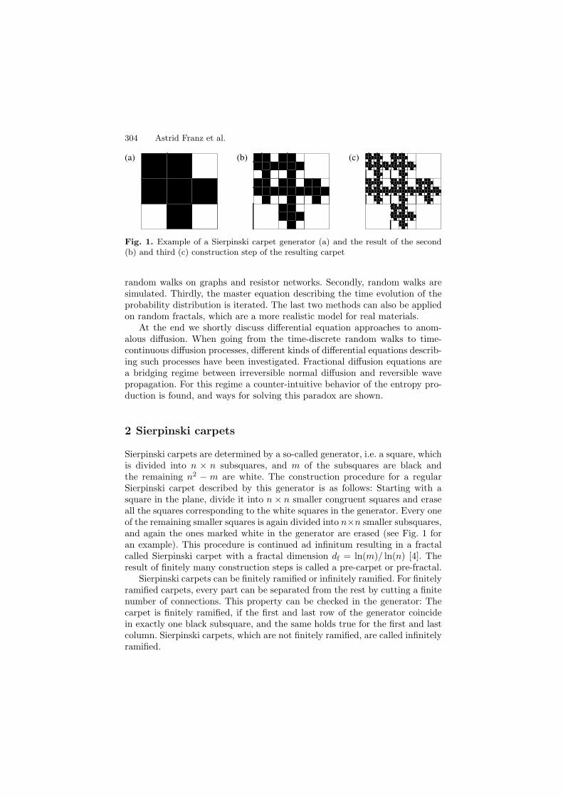
304 Astrid Franz et al.
(a) (b) (c)
Fig. 1. Example of a Sierpinski carpet generator (a) and the result of the second(b) and third (c) construction step of the resulting carpet
random walks on graphs and resistor networks. Secondly, random walks aresimulated. Thirdly, the master equation describing the time evolution of theprobability distribution is iterated. The last two methods can also be appliedon random fractals, which are a more realistic model for real materials.
At the end we shortly discuss differential equation approaches to anom-alous diffusion. When going from the time-discrete random walks to time-continuous diffusion processes, different kinds of differential equations describ-ing such processes have been investigated. Fractional diffusion equations area bridging regime between irreversible normal diffusion and reversible wavepropagation. For this regime a counter-intuitive behavior of the entropy pro-duction is found, and ways for solving this paradox are shown.
2 Sierpinski carpets
Sierpinski carpets are determined by a so-called generator, i.e. a square, whichis divided into n × n subsquares, and m of the subsquares are black andthe remaining n2 − m are white. The construction procedure for a regularSierpinski carpet described by this generator is as follows: Starting with asquare in the plane, divide it into n× n smaller congruent squares and eraseall the squares corresponding to the white squares in the generator. Every oneof the remaining smaller squares is again divided into n×n smaller subsquares,and again the ones marked white in the generator are erased (see Fig. 1 foran example). This procedure is continued ad infinitum resulting in a fractalcalled Sierpinski carpet with a fractal dimension df = ln(m)/ ln(n) [4]. Theresult of finitely many construction steps is called a pre-carpet or pre-fractal.
Sierpinski carpets can be finitely ramified or infinitely ramified. For finitelyramified carpets, every part can be separated from the rest by cutting a finitenumber of connections. This property can be checked in the generator: Thecarpet is finitely ramified, if the first and last row of the generator coincidein exactly one black subsquare, and the same holds true for the first and lastcolumn. Sierpinski carpets, which are not finitely ramified, are called infinitelyramified.
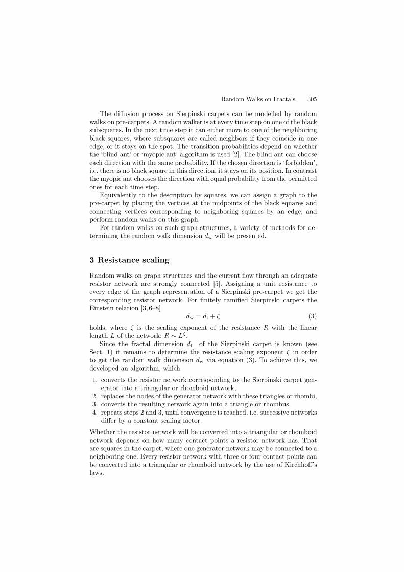
Random Walks on Fractals 305
The diffusion process on Sierpinski carpets can be modelled by randomwalks on pre-carpets. A random walker is at every time step on one of the blacksubsquares. In the next time step it can either move to one of the neighboringblack squares, where subsquares are called neighbors if they coincide in oneedge, or it stays on the spot. The transition probabilities depend on whetherthe ‘blind ant’ or ‘myopic ant’ algorithm is used [2]. The blind ant can chooseeach direction with the same probability. If the chosen direction is ‘forbidden’,i.e. there is no black square in this direction, it stays on its position. In contrastthe myopic ant chooses the direction with equal probability from the permittedones for each time step.
Equivalently to the description by squares, we can assign a graph to thepre-carpet by placing the vertices at the midpoints of the black squares andconnecting vertices corresponding to neighboring squares by an edge, andperform random walks on this graph.
For random walks on such graph structures, a variety of methods for de-termining the random walk dimension dw will be presented.
3 Resistance scaling
Random walks on graph structures and the current flow through an adequateresistor network are strongly connected [5]. Assigning a unit resistance toevery edge of the graph representation of a Sierpinski pre-carpet we get thecorresponding resistor network. For finitely ramified Sierpinski carpets theEinstein relation [3, 6–8]
dw = df + ζ (3)
holds, where ζ is the scaling exponent of the resistance R with the linearlength L of the network: R ∼ Lζ .
Since the fractal dimension df of the Sierpinski carpet is known (seeSect. 1) it remains to determine the resistance scaling exponent ζ in orderto get the random walk dimension dw via equation (3). To achieve this, wedeveloped an algorithm, which
1. converts the resistor network corresponding to the Sierpinski carpet gen-erator into a triangular or rhomboid network,
2. replaces the nodes of the generator network with these triangles or rhombi,3. converts the resulting network again into a triangle or rhombus,4. repeats steps 2 and 3, until convergence is reached, i.e. successive networks
differ by a constant scaling factor.
Whether the resistor network will be converted into a triangular or rhomboidnetwork depends on how many contact points a resistor network has. Thatare squares in the carpet, where one generator network may be connected to aneighboring one. Every resistor network with three or four contact points canbe converted into a triangular or rhomboid network by the use of Kirchhoff’slaws.
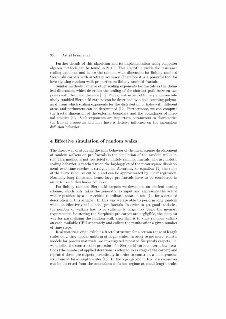
306 Astrid Franz et al.
Further details of this algorithm and its implementation using computeralgebra methods can be found in [9, 10]. This algorithm yields the resistancescaling exponent and hence the random walk dimension for finitely ramifiedSierpinski carpets with arbitrary accuracy. Therefore it is a powerful tool forinvestigating random walk properties on finitely ramified fractals.
Similar methods can give other scaling exponents for fractals as the chem-ical dimension, which describes the scaling of the shortest path between twopoints with the linear distance [11]. The pore structure of finitely and even infi-nitely ramified Sierpinski carpets can be described by a hole-counting polyno-mial, from which scaling exponents for the distribution of holes with differentareas and perimeters can be determined [12]. Furthermore, we can computethe fractal dimension of the external boundary and the boundaries of inter-nal cavities [13]. Such exponents are important parameters to characterizethe fractal properties and may have a decisive influence on the anomalousdiffusion behavior.
4 Effective simulation of random walks
The direct way of studying the time behavior of the mean square displacementof random walkers on pre-fractals is the simulation of the random walks it-self. This method is not restricted to finitely ramified fractals. The asymptoticscaling behavior is reached when the log-log-plot of the mean square displace-ment over time reaches a straight line. According to equation (1) the slopeof the curve is equivalent to γ and can be approximated by linear regression.Normally long times and hence large pre-fractals have to be considered inorder to reach this linear behavior.
For finitely ramified Sierpinski carpets we developed an efficient storingscheme, which only takes the generator as input and represents the actualwalker position by a hierarchical coordinate notation (see [14] for a detaileddescription of this scheme). In this way we are able to perform long randomwalks on effectively unbounded pre-fractals. In order to get good statistics,the number of walkers has to be sufficiently large, too. Since the memoryrequirements for storing the Sierpinski pre-carpet are negligible, the simplestway for parallelizing the random walk algorithm is to start random walkerson each available CPU separately and collect the results after a given numberof time steps.
Real materials often exhibit a fractal structure for a certain range of lengthscales only, they appear uniform at larger scales. In order to get more realisticmodels for porous materials, we investigated repeated Sierpinski carpets, i.e.we applied the construction procedure for Sierpinski carpets over a few itera-tions (the number of applied iterations is referred to as stage of the carpet) andrepeated these pre-carpets periodically in order to construct a homogeneousstructure at large length scales [15]. In the log-log-plot in Fig. 2 a cross-overcan be observed from the anomalous diffusion regime at small length scales
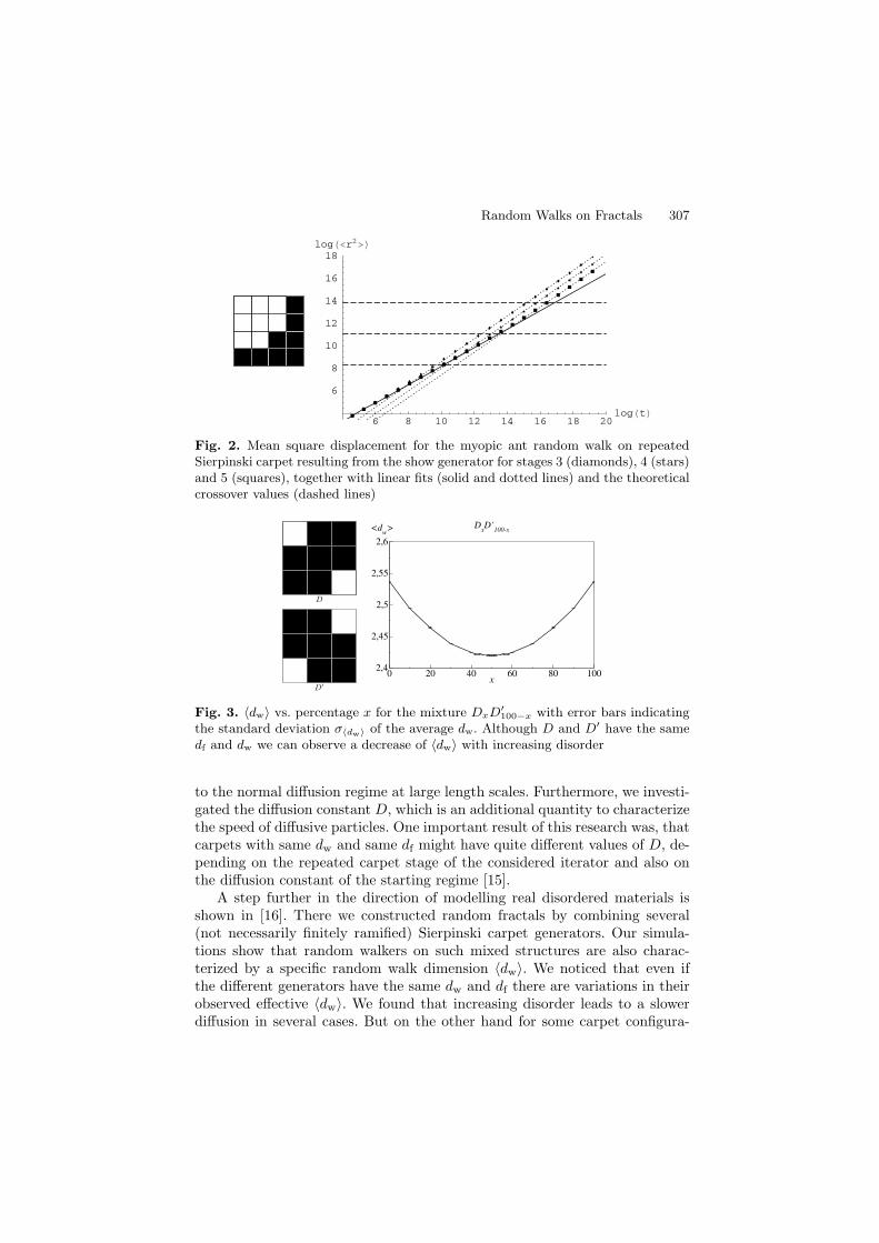
Random Walks on Fractals 307
6 8 10 12 14 16 18 20logt
6
8
10
12
14
16
18logr2
Fig. 2. Mean square displacement for the myopic ant random walk on repeatedSierpinski carpet resulting from the show generator for stages 3 (diamonds), 4 (stars)and 5 (squares), together with linear fits (solid and dotted lines) and the theoreticalcrossover values (dashed lines)
0 20 40 60 80 100x
2,4
2,45
2,5
2,55
2,6
<dw> D
xD’
100-x
D
D′
Fig. 3. 〈dw〉 vs. percentage x for the mixture DxD′100−x with error bars indicating
the standard deviation σ〈dw〉 of the average dw. Although D and D′ have the samedf and dw we can observe a decrease of 〈dw〉 with increasing disorder
to the normal diffusion regime at large length scales. Furthermore, we investi-gated the diffusion constant D, which is an additional quantity to characterizethe speed of diffusive particles. One important result of this research was, thatcarpets with same dw and same df might have quite different values of D, de-pending on the repeated carpet stage of the considered iterator and also onthe diffusion constant of the starting regime [15].
A step further in the direction of modelling real disordered materials isshown in [16]. There we constructed random fractals by combining several(not necessarily finitely ramified) Sierpinski carpet generators. Our simula-tions show that random walkers on such mixed structures are also charac-terized by a specific random walk dimension 〈dw〉. We noticed that even ifthe different generators have the same dw and df there are variations in theirobserved effective 〈dw〉. We found that increasing disorder leads to a slowerdiffusion in several cases. But on the other hand for some carpet configura-
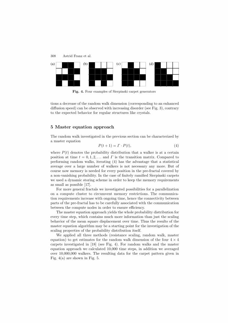
308 Astrid Franz et al.
(a) (b) (c) (d)
Fig. 4. Four examples of Sierpinski carpet generators
tions a decrease of the random walk dimension (corresponding to an enhanceddiffusion speed) can be observed with increasing disorder (see Fig. 3), contraryto the expected behavior for regular structures like crystals.
5 Master equation approach
The random walk investigated in the previous section can be characterized bya master equation
P (t+ 1) = Γ · P (t), (4)
where P (t) denotes the probability distribution that a walker is at a certainposition at time t = 0, 1, 2, . . . and Γ is the transition matrix. Compared toperforming random walks, iterating (4) has the advantage that a statisticalaverage over a large number of walkers is not necessary any more. But ofcourse now memory is needed for every position in the pre-fractal covered bya non-vanishing probability. In the case of finitely ramified Sierpinski carpetswe used a dynamic storing scheme in order to keep the memory requirementsas small as possible [17].
For more general fractals we investigated possibilities for a parallelizationon a compute cluster to circumvent memory restrictions. The communica-tion requirements increase with ongoing time, hence the connectivity betweenparts of the pre-fractal has to be carefully associated with the communicationbetween the compute nodes in order to ensure efficiency.
The master equation approach yields the whole probability distribution forevery time step, which contains much more information than just the scalingbehavior of the mean square displacement over time. Thus the results of themaster equation algorithm may be a starting point for the investigation of thescaling properties of the probability distribution itself.
We applied all three methods (resistance scaling, random walk, masterequation) to get estimates for the random walk dimension of the four 4 × 4carpets investigated in [18] (see Fig. 4). For random walks and the masterequation approach we calculated 10,000 time steps, in addition we averagedover 10,000,000 walkers. The resulting data for the carpet pattern given inFig. 4(a) are shown in Fig. 5.
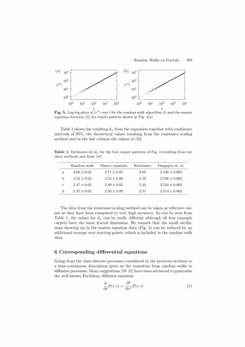
Random Walks on Fractals 309
100
101
102
103
100 101 102 103 104
(a)
t
〈r2〉
100
101
102
103
100 101 102 103 104
(b)
t
〈r2〉
Fig. 5. Log-log-plots of 〈r2〉 over t for the random walk algorithm (i) and the masterequation iteration (ii) for carpet pattern shown in Fig. 4(a)
Table 1 shows the resulting dw from the regression together with confidenceintervals of 95%, the theoretical values resulting from the resistance scalingmethod and in the last column the values of [18].
Table 1. Estimates for dw for the four carpet patterns of Fig. 4 resulting from ourthree methods and from [18]
Random walk Master equation Resistance Dasgupta et. al.
a 2.68 ± 0.02 2.71 ± 0.05 2.66 2.538 ± 0.002
b 2.52 ± 0.02 2.52 ± 0.06 2.58 2.528 ± 0.002
c 2.47 ± 0.02 2.49 ± 0.05 2.49 2.524 ± 0.002
d 2.47 ± 0.02 2.50 ± 0.09 2.51 2.514 ± 0.002
The data from the resistance scaling method can be taken as reference val-ues as they have been computed to very high accuracy. As can be seen fromTable 1, the values for dw can be really different although all four examplecarpets have the same fractal dimension. We remark that the small oscilla-tions showing up in the master equation data (Fig. 5) can be reduced by anadditional average over starting points, which is included in the random walkdata.
6 Corresponding differential equations
Going from the time-discrete processes considered in the previous sections toa time-continuous description gives us the transition from random walks todiffusion processes. Many suggestions [19–21] have been advanced to generalizethe well-known Euclidean diffusion equation
∂
∂tP (r, t) =
∂2
∂r2P (r, t) (5)
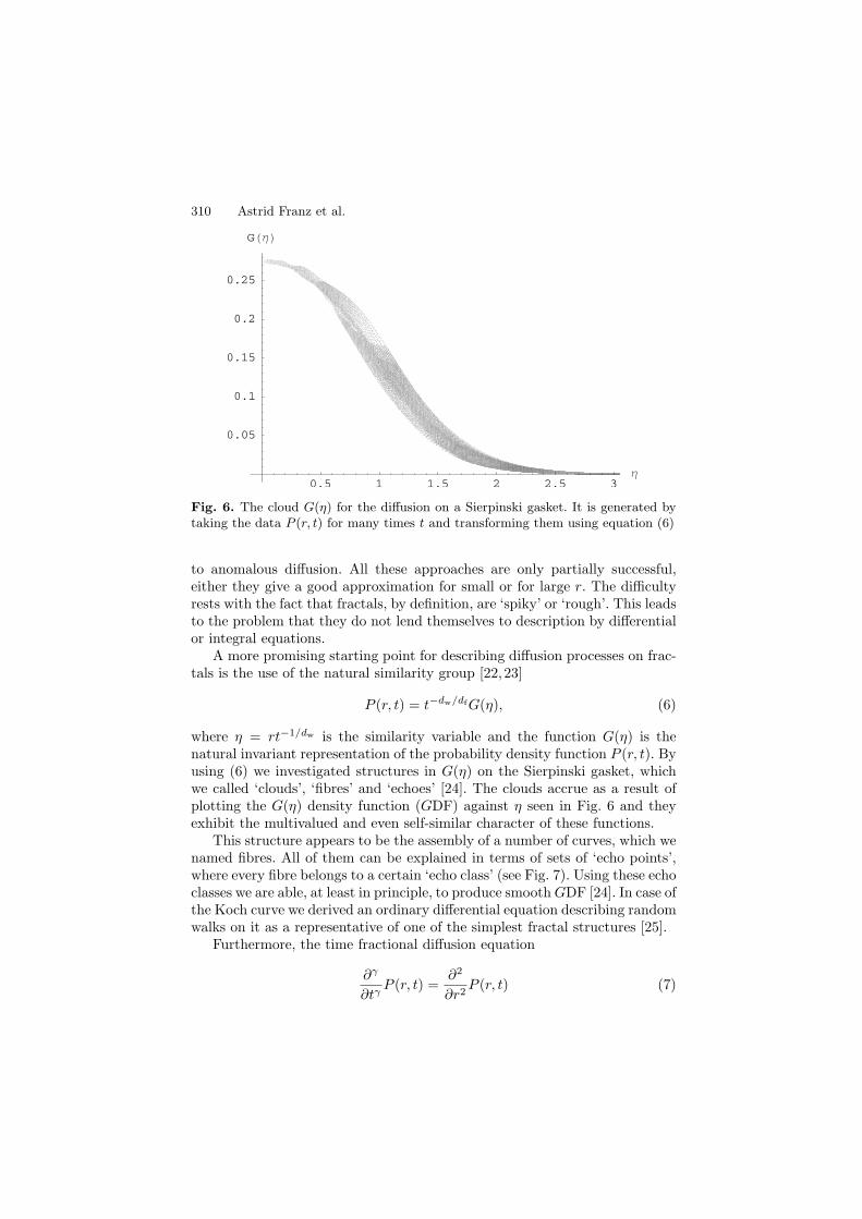
310 Astrid Franz et al.
0.5 1 1.5 2 2.5 3Η
0.05
0.1
0.15
0.2
0.25
GΗ
Fig. 6. The cloud G(η) for the diffusion on a Sierpinski gasket. It is generated bytaking the data P (r, t) for many times t and transforming them using equation (6)
to anomalous diffusion. All these approaches are only partially successful,either they give a good approximation for small or for large r. The difficultyrests with the fact that fractals, by definition, are ‘spiky’ or ‘rough’. This leadsto the problem that they do not lend themselves to description by differentialor integral equations.
A more promising starting point for describing diffusion processes on frac-tals is the use of the natural similarity group [22,23]
P (r, t) = t−dw/dfG(η), (6)
where η = rt−1/dw is the similarity variable and the function G(η) is thenatural invariant representation of the probability density function P (r, t). Byusing (6) we investigated structures in G(η) on the Sierpinski gasket, whichwe called ‘clouds’, ‘fibres’ and ‘echoes’ [24]. The clouds accrue as a result ofplotting the G(η) density function (GDF) against η seen in Fig. 6 and theyexhibit the multivalued and even self-similar character of these functions.
This structure appears to be the assembly of a number of curves, which wenamed fibres. All of them can be explained in terms of sets of ‘echo points’,where every fibre belongs to a certain ‘echo class’ (see Fig. 7). Using these echoclasses we are able, at least in principle, to produce smoothGDF [24]. In case ofthe Koch curve we derived an ordinary differential equation describing randomwalks on it as a representative of one of the simplest fractal structures [25].
Furthermore, the time fractional diffusion equation
∂γ
∂tγP (r, t) =
∂2
∂r2P (r, t) (7)
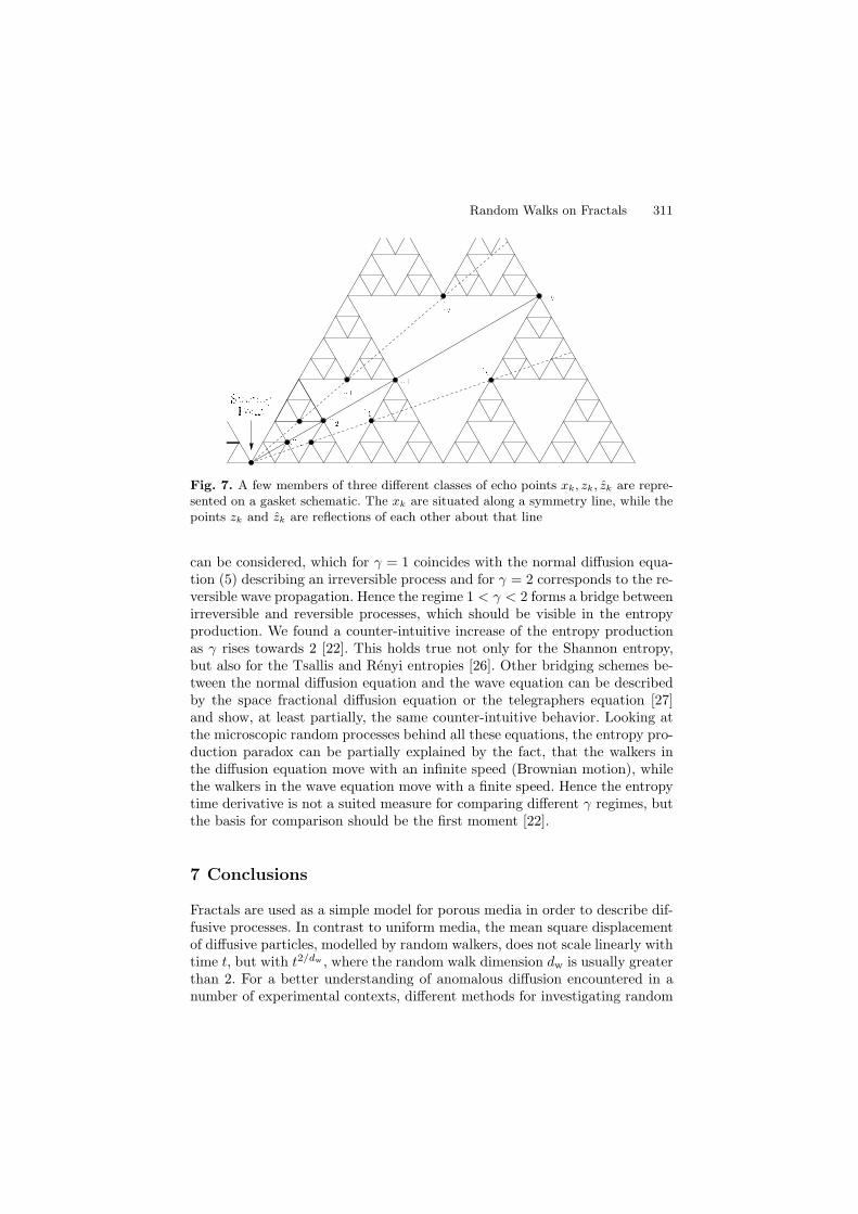
Random Walks on Fractals 311
Fig. 7. A few members of three different classes of echo points xk, zk, zk are repre-sented on a gasket schematic. The xk are situated along a symmetry line, while thepoints zk and zk are reflections of each other about that line
can be considered, which for γ = 1 coincides with the normal diffusion equa-tion (5) describing an irreversible process and for γ = 2 corresponds to the re-versible wave propagation. Hence the regime 1 < γ < 2 forms a bridge betweenirreversible and reversible processes, which should be visible in the entropyproduction. We found a counter-intuitive increase of the entropy productionas γ rises towards 2 [22]. This holds true not only for the Shannon entropy,but also for the Tsallis and Renyi entropies [26]. Other bridging schemes be-tween the normal diffusion equation and the wave equation can be describedby the space fractional diffusion equation or the telegraphers equation [27]and show, at least partially, the same counter-intuitive behavior. Looking atthe microscopic random processes behind all these equations, the entropy pro-duction paradox can be partially explained by the fact, that the walkers inthe diffusion equation move with an infinite speed (Brownian motion), whilethe walkers in the wave equation move with a finite speed. Hence the entropytime derivative is not a suited measure for comparing different γ regimes, butthe basis for comparison should be the first moment [22].
7 Conclusions
Fractals are used as a simple model for porous media in order to describe dif-fusive processes. In contrast to uniform media, the mean square displacementof diffusive particles, modelled by random walkers, does not scale linearly withtime t, but with t2/dw , where the random walk dimension dw is usually greaterthan 2. For a better understanding of anomalous diffusion encountered in anumber of experimental contexts, different methods for investigating random
312 Astrid Franz et al.
walks on fractals were studied. We determined the scaling exponent of themean square displacement of the walkers with time as an important quantityto characterize diffusion properties. Furthermore we developed techniques tocalculate further properties of diffusion on fractals, i.e. the resistance scalingexponent, chemical dimension or the pore structure.
Some of the methods additionally yield the whole probability distributionfor every time step, containing much more information than just the scalingbehavior of the mean square displacement. Going to a time-continuous de-scription, the time evolution of the probability distribution can be describedby differential equations. In case of fractional differential equations, they area bridging scheme between the irreversible normal diffusion equation and thereversible wave equation. However, the entropy production is no adapted quan-tity characterizing this regime.
Acknowledgment
We want to thank C. Essex, M. Davison, X. Li, and S. Tarafdar for helpfuldiscussions during our extended collaborations.
References
1. B. B. Mandelbrot. Fractals - Form, Chance and Dimension. W. H. Freeman,San Francisco, 1977.
2. S. Havlin and D. Ben-Avraham. Diffusion in disordered media. Adv. Phys.,36(6):695–798, 1987.
3. A. Bunde and S. Havlin, editors. Fractals and Disordered Systems. Springer,Berlin, Heidelberg, New-York, 2nd edition edition, 1996.
4. K. J. Falconer. Techniques in fractal geometry. John Wiley & Sons Ltd, Chich-ester, 1997.
5. P. Tetali. Random walks and the effective resistance of networks. J. Theor.Prob., 4(1):101–109, 1991.
6. J. A. Given and B. B. Mandelbrot. Diffusion on fractal lattices and the fractalEinstein relation. J. Phys. B: At. Mol. Opt. Phys., 16:L565–L569, 1983.
7. M. T. Barlow, R. F. Bass, and J. D. Sherwood. Resistance and spectral dimen-sion of Sierpinski carpets. J. Phys. A: Math. Gen., 23(6):L253–L238, 1990.
8. A. Franz, C. Schulzky, and K. H. Hoffmann. The Einstein relation for finitelyramified Sierpinski carpets. Nonlinearity, 14(5):1411–1418, 2001.
9. C. Schulzky, A. Franz, and K. H. Hoffmann. Resistance scaling and random walkdimensions for finitely ramified Sierpinski carpets. SIGSAM Bulletin, 34(3):1–8,2000.
10. A. Franz, C. Schulzky, S. Seeger, and K. H. Hoffmann. Diffusion on fractals –efficient algorithms to compute the random walk dimension. In J. M. Black-ledge, A. K. Evans, and M. J. Turner, editors, Fractal Geometry: MathematicalMethods, Algorithms, Applications, IMA Conference Proceedings, pages 52–67.Horwood Publishing Ltd., Chichester, West Sussex, 2002.
Random Walks on Fractals 313
11. A. Franz, C. Schulzky, and K. H. Hoffmann. Using computer algebra meth-ods to determine the chemical dimension of finitely ramified Sierpinski carpets.SIGSAM Bulletin, 36(2):18–30, 2002.
12. A. Franz, C. Schulzky, S. Tarafdar, and K. H. Hoffmann. The pore structure ofSierpinski carpets. J. Phys. A: Math. Gen., 34(42):8751–8765, 2001.
13. P. Blaudeck, S. Seeger, C. Schulzky, K. H. Hoffmann, T. Dutta, and S. Tarafdar.The coastline and lake shores of a fractal island. J. Phys. A: Math. Gen.,39:1609–1618, 2006.
14. S. Seeger, A. Franz, C. Schulzky, and K. H. Hoffmann. Random walks on finitelyramified Sierpinski carpets. Comp. Phys. Comm., 134(3):307–316, 2001.
15. S. Tarafdar, A. Franz, S. Schulzky, and K. H. Hoffmann. Modelling porousstructures by repeated Sierpinski carpets. Physica A, 292(1-4):1–8, 2001.
16. D. H. N. Anh, K. H. Hoffmann, S. Seeger, and S. Tarafdar. Diffusion in disor-dered fractals. Europhys. Lett., 70(1):109–115, 2005.
17. A. Franz, C. Schulzky, S. Seeger, and K. H. Hoffmann. An efficient implementa-tion of the exact enumeration method for random walks on Sierpinski carpets.Fractals, 8(2):155–161, 2000.
18. R. Dasgupta, T. K. Ballabh, and S. Tarafdar. Scaling exponents for randomwalks on Sierpinski carpets and number of distinct sites visited: A new algorithmfor infinite fractal lattices. J. Phys. A: Math. Gen., 32(37):6503–6516, 1999.
19. B. O’Shaughnessy and I. Procaccia. Analytical solutions for diffusion on fractalobjects. Phys. Rev. Lett., 54(5):455–458, 1985.
20. M. Giona and H. E. Roman. Fractional diffusion equation for transport phe-nomena in random media. Physica A, 185:87–97, 1992.
21. R. Metzler, W. G. Glockle, and T. F. Nonnemacher. Fractional model equationfor anomalous diffusion. Physica A, 211(1):13–24, 1994.
22. K. H. Hoffmann, C. Essex, and C. Schulzky. Fractional diffusion and entropyproduction. J. Non-Equilib. Thermodyn., 23(2):166–175, 1998.
23. C. Schulzky, C. Essex, M. Davison, A. Franz, and K. H. Hoffmann. The similaritygroup and anomalous diffusion equations. J. Phys. A: Math. Gen., 33(31):5501–5511, 2000.
24. M. Davison, C. Essex, C. Schulzky, A. Franz, and K. H. Hoffmann. Clouds,fibres and echoes: a new approach to studying random walks on fractals. J.Phys. A: Math. Gen., 34(20):L289–L296, 2001.
25. C. Essex, M. Davison, C. Schulzky, A. Franz, and K. H. Hoffmann. The differ-ential equation describing random walks on the Koch curve. J. Phys. A: Math.Gen., 34(41):8397–8406, 2001.
26. C. Essex, C. Schulzky, A. Franz, and K. H. Hoffmann. Tsallis and Renyi en-tropies in fractional diffusion and entropy production. Physica A, 284(1-4):299–308, 2000.
27. X. Li, C. Essex, M. Davison, K. H. Hoffmann, and C. Schulzky. Fractionaldiffusion, irreversibility and entropy. J. Non-Equilib. Thermodyn., 28(3):279–291, 2003.

Lyapunov Instabilities of Extended Systems
Hong-liu Yang and Gunter Radons
Technische Universitat Chemnitz, Institut fur Physik09107 Chemnitz, [email protected]
1 Introduction
One of the most successful theories in modern science is statistical mechanics,which allows us to understand the macroscopic (thermodynamic) propertiesof matter from a statistical analysis of the microscopic (mechanical) behav-ior of the constituent particles. In spite of this, using certain probabilisticassumptions such as Boltzmann’s Stosszahlansatz causes the lack of a firmfoundation of this theory, especially for non-equilibrium statistical mechanics.Fortunately, the concept of chaotic dynamics developed in the 20th century [1]is a good candidate for accounting for these difficulties. Instead of the proba-bilistic assumptions, the dynamical instability of trajectories can make avail-able the necessary fast loss of time correlations, ergodicity, mixing and otherdynamical randomness [2]. It is generally expected that dynamical instabilityis at the basis of macroscopic transport phenomena and that one can find cer-tain connections between them. Some beautiful theories in this direction werealready developed in the past decade. Examples are the escape-rate formalismby Gaspard and Nicolis [3, 4] and the Gaussian thermostat method by Nose,Hoover, Evans, Morriss and others [5,6], where the Lyapunov exponents wererelated to certain transport coefficients.
Very recently, molecular dynamics simulations on hard-core systems re-vealed the existence of regular collective perturbations corresponding to thesmallest positive Lyapunov exponents (LEs), named hydrodynamic Lyapunovmodes [7]. This provides a new possibility for the connection between Lya-punov vectors, a quantity characterizing the dynamical instability of trajec-tories, and macroscopic transport properties. A lot of work [8–14] has beendone to identify this phenomenon and to find out its origin. The appearanceof these modes is commonly thought to be due to the conservation of certainquantities in the systems studied [8–12]. A natural consequence of this expec-tation is that the appearance of such modes might not be an exclusive featureof hard-core systems and might be generic to a large class of Hamiltonian
316 Hong-liu Yang and Gunter Radons
systems. However, until very recently, these modes have only been identifiedin the computer simulations of hard-core systems [8, 14].
Here we review our current results on Lyapunov spectra and Lyapunovvectors (LVs) of various extended systems with continuous symmetries, espe-cially on the identification and characterization of hydrodynamic Lyapunovmodes. The major part of our discussion is devoted to the study of Lennard-Jones fluids in one- and two-dimensional spaces, wherein the HLMs are, forthe first time, identified in systems with soft-potential interactions [15, 16].By using the newly introduced LV correlation functions, we demonstrate thatthe LVs with λ ≈ 0 are highly dominated by a few components with lowwave numbers, which implies the existence of hydrodynamic Lyapunov modes(HLMs) in soft-potential systems. Despite the wave-like character of the LVs,no step-like structure exists in the Lyapunov spectrum of the systems studiedhere, in contrast to the hard-core case. Further numerical simulations showthat the finite-time Lyapunov exponents fluctuate strongly. Studies on dy-namical LV structure factors conclude that HLMs in Lennard-Jones fluidsare propagating. We also briefly outline our current results on the universalfeatures of HLMs in a class of spatially extended systems with continuoussymmetries. HLMs in Hamiltonian and dissipative systems are found to differboth in respect of spatial structure and in the dynamical evolution. Details ofthese investigations can be found in our publications [17–19].
2 Numerical method for determining Lyapunovexponents and vectors
2.1 Standard method
The equations of motion for a many-body system may always be written asa set of first order differential equations Γ (t) = F (Γ (t)), where Γ is a vectorin the D-dimensional phase space. The tangent space dynamics describinginfinitesimal perturbations around a reference trajectory Γ (t) is given by
δΓ =M(Γ (t)) · δΓ (1)
with the Jacobian M = dFdΓ . The time averaged expansion or contraction
rates of δΓ (t) are given by the Lyapunov exponents [1]. For a D−dimensionaldynamical system there exist in total D Lyapunov exponents for D differentdirections in tangent space. The orientation vectors of these directions are theLyapunov vectors e(α)(t), α = 1,· · · ,D.
For the calculation of the Lyapunov exponents and vectors the offsetvectors have to be reorthogonalized periodically, either by means of Gram-Schmidt orthogonalization or QR decomposition [20, 21]. To obtain scientif-ically useful results, one needs large particle numbers and long integrationtimes for the calculation of certain long time averages. This enforces the use
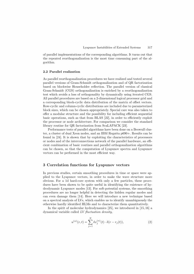
Lyapunov Instabilities of Extended Systems 317
of parallel implementations of the corresponding algorithms. It turns out thatthe repeated reorthogonalization is the most time consuming part of the al-gorithm.
2.2 Parallel realization
As parallel reorthogonalization procedures we have realized and tested severalparallel versions of Gram-Schmidt orthogonalization and of QR factorizationbased on blockwise Householder reflection. The parallel version of classicalGram-Schmidt (CGS) orthogonalization is enriched by a reorthogonalizationtest which avoids a loss of orthogonality by dynamically using iterated CGS.All parallel procedures are based on a 2-dimensional logical processor grid anda corresponding block-cyclic data distribution of the matrix of offset vectors.Row-cyclic and column-cyclic distributions are included due to parameterizedblock sizes, which can be chosen appropriately. Special care was also taken tooffer a modular structure and the possibility for including efficient sequentialbasic operations, such as that from BLAS [22], in order to efficiently exploitthe processor or node architecture. For comparison we consider the standardlibrary routine for QR factorization from ScaLAPACK [23].
Performance tests of parallel algorithms have been done on a Beowulf clus-ter, a cluster of dual Xeon nodes, and an IBM Regatta p690+. Results can befound in [24]. It is shown that by exploiting the characteristics of processorsor nodes and of the interconnections network of the parallel hardware, an effi-cient combination of basic routines and parallel orthogonalization algorithmscan be chosen, so that the computation of Lyapunov spectra and Lyapunovvectors can be performed in the most efficient way.
3 Correlation functions for Lyapunov vectors
In previous studies, certain smoothing procedures in time or space were ap-plied to the Lyapunov vectors, in order to make the wave structure moreobvious. For a 1d hard-core system with only a few particles, these proce-dures have been shown to be quite useful in identifying the existence of hy-drodynamic Lyapunov modes [13]. For soft-potential systems, the smoothingprocedures are no longer helpful in detecting the hidden regular modes andcan even damage them [14]. Here we will introduce a new technique basedon a spectral analysis of LVs, which enables us to identify unambiguously theotherwise hardly identified HLMs and to characterize them quantitatively.
In the spirit of molecular hydrodynamics [25], we introduced in [15, 16] adynamical variable called LV fluctuation density,
u(α)(r, t) =
N∑
j=1
δx(α)j (t) · δ(r − rj(t)), (2)
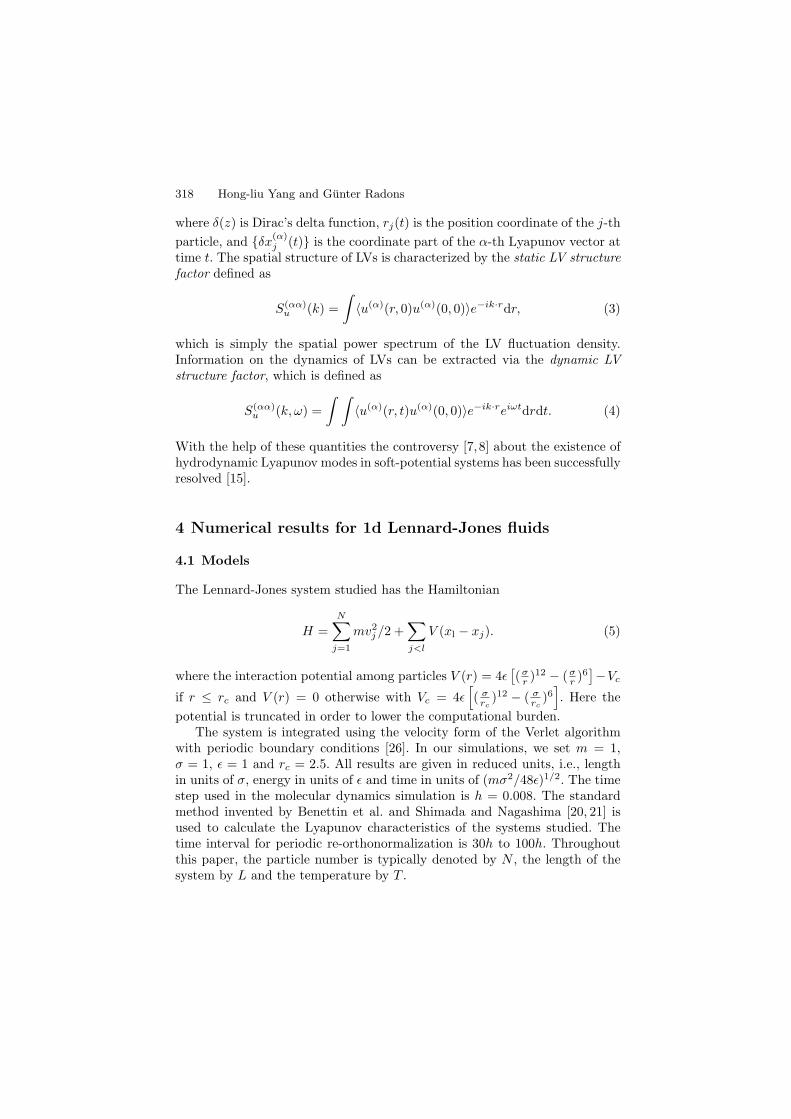
318 Hong-liu Yang and Gunter Radons
where δ(z) is Dirac’s delta function, rj(t) is the position coordinate of the j-th
particle, and δx(α)j (t) is the coordinate part of the α-th Lyapunov vector at
time t. The spatial structure of LVs is characterized by the static LV structurefactor defined as
S(αα)u (k) =
∫〈u(α)(r, 0)u(α)(0, 0)〉e−ik·rdr, (3)
which is simply the spatial power spectrum of the LV fluctuation density.Information on the dynamics of LVs can be extracted via the dynamic LVstructure factor, which is defined as
S(αα)u (k, ω) =
∫ ∫〈u(α)(r, t)u(α)(0, 0)〉e−ik·reiωtdrdt. (4)
With the help of these quantities the controversy [7,8] about the existence ofhydrodynamic Lyapunov modes in soft-potential systems has been successfullyresolved [15].
4 Numerical results for 1d Lennard-Jones fluids
4.1 Models
The Lennard-Jones system studied has the Hamiltonian
H =
N∑
j=1
mv2j /2 +∑
j<l
V (xl − xj). (5)
where the interaction potential among particles V (r) = 4ǫ[(σ
r )12 − (σr )6
]−Vc
if r ≤ rc and V (r) = 0 otherwise with Vc = 4ǫ[( σ
rc)12 − ( σ
rc)6]. Here the
potential is truncated in order to lower the computational burden.The system is integrated using the velocity form of the Verlet algorithm
with periodic boundary conditions [26]. In our simulations, we set m = 1,σ = 1, ǫ = 1 and rc = 2.5. All results are given in reduced units, i.e., lengthin units of σ, energy in units of ǫ and time in units of (mσ2/48ǫ)1/2. The timestep used in the molecular dynamics simulation is h = 0.008. The standardmethod invented by Benettin et al. and Shimada and Nagashima [20, 21] isused to calculate the Lyapunov characteristics of the systems studied. Thetime interval for periodic re-orthonormalization is 30h to 100h. Throughoutthis paper, the particle number is typically denoted by N , the length of thesystem by L and the temperature by T .
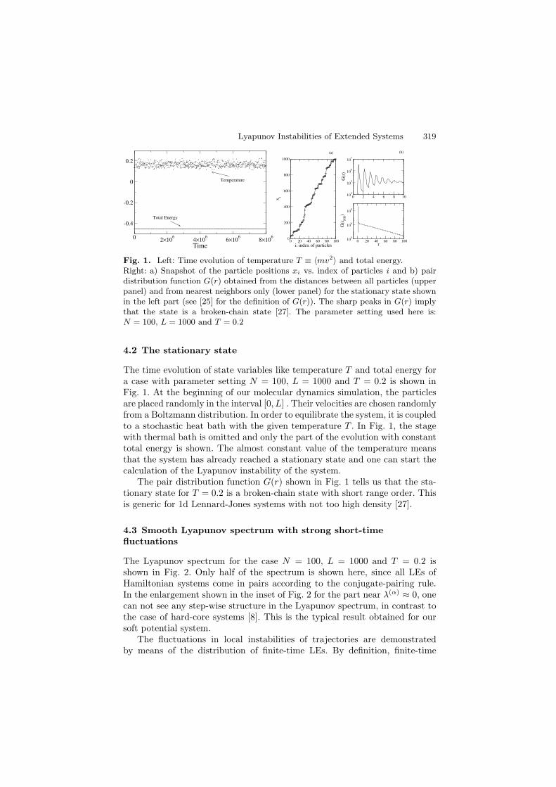
Lyapunov Instabilities of Extended Systems 319
0 2×10⁶
4×10⁶
6×10⁶
8×10⁶
Time
-0.4
-0.2
0
0.2
Temperature
Total Energy
0 20 40 60 80 100i: index of particles
0
200
400
600
800
1000
x i 0 2 4 6 8 10104
105
106
107
G(r
)
0 20 40 60 80 100r
104
106
108
G(r
NN
)
(a) (b)
Fig. 1. Left: Time evolution of temperature T ≡ 〈mv2〉 and total energy.Right: a) Snapshot of the particle positions xi vs. index of particles i and b) pairdistribution function G(r) obtained from the distances between all particles (upperpanel) and from nearest neighbors only (lower panel) for the stationary state shownin the left part (see [25] for the definition of G(r)). The sharp peaks in G(r) implythat the state is a broken-chain state [27]. The parameter setting used here is:N = 100, L = 1000 and T = 0.2
4.2 The stationary state
The time evolution of state variables like temperature T and total energy fora case with parameter setting N = 100, L = 1000 and T = 0.2 is shown inFig. 1. At the beginning of our molecular dynamics simulation, the particlesare placed randomly in the interval [0, L] . Their velocities are chosen randomlyfrom a Boltzmann distribution. In order to equilibrate the system, it is coupledto a stochastic heat bath with the given temperature T . In Fig. 1, the stagewith thermal bath is omitted and only the part of the evolution with constanttotal energy is shown. The almost constant value of the temperature meansthat the system has already reached a stationary state and one can start thecalculation of the Lyapunov instability of the system.
The pair distribution function G(r) shown in Fig. 1 tells us that the sta-tionary state for T = 0.2 is a broken-chain state with short range order. Thisis generic for 1d Lennard-Jones systems with not too high density [27].
4.3 Smooth Lyapunov spectrum with strong short-timefluctuations
The Lyapunov spectrum for the case N = 100, L = 1000 and T = 0.2 isshown in Fig. 2. Only half of the spectrum is shown here, since all LEs ofHamiltonian systems come in pairs according to the conjugate-pairing rule.In the enlargement shown in the inset of Fig. 2 for the part near λ(α) ≈ 0, onecan not see any step-wise structure in the Lyapunov spectrum, in contrast tothe case of hard-core systems [8]. This is the typical result obtained for oursoft potential system.
The fluctuations in local instabilities of trajectories are demonstratedby means of the distribution of finite-time LEs. By definition, finite-time
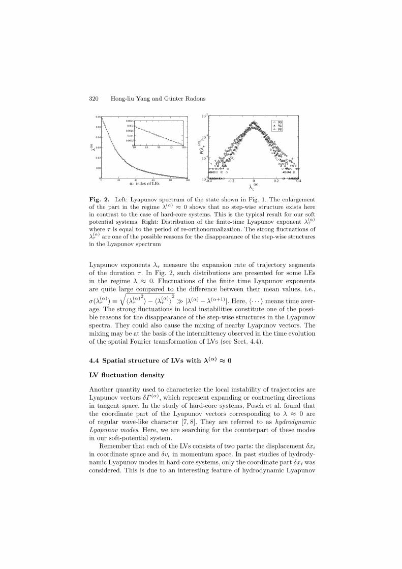
320 Hong-liu Yang and Gunter Radons
0 20 40 60 80 100
α: index of LEs
0
0.01
0.02
0.03
0.04
0.05
0.06
λ(α
)
80 85 90 95 1000
0.0005
0.001
0.0015
0.002
0.0025
-0.4 -0.2 0 0.2 0.4
λτ
(α)
10-5
10-4
10-3
10-2
P(λ
τ(α) )
909498
Fig. 2. Left: Lyapunov spectrum of the state shown in Fig. 1. The enlargementof the part in the regime λ(α) ≈ 0 shows that no step-wise structure exists herein contrast to the case of hard-core systems. This is the typical result for our softpotential systems. Right: Distribution of the finite-time Lyapunov exponent λ
(α)τ
where τ is equal to the period of re-orthonormalization. The strong fluctuations ofλ
(α)τ are one of the possible reasons for the disappearance of the step-wise structures
in the Lyapunov spectrum
Lyapunov exponents λτ measure the expansion rate of trajectory segmentsof the duration τ . In Fig. 2, such distributions are presented for some LEsin the regime λ ≈ 0. Fluctuations of the finite time Lyapunov exponentsare quite large compared to the difference between their mean values, i.e.,
σ(λ(α)τ ) ≡
√〈λ(α)
τ
2〉 − 〈λ(α)
τ 〉2≫ |λ(α)− λ(α+1)|. Here, 〈· · · 〉 means time aver-
age. The strong fluctuations in local instabilities constitute one of the possi-ble reasons for the disappearance of the step-wise structures in the Lyapunovspectra. They could also cause the mixing of nearby Lyapunov vectors. Themixing may be at the basis of the intermittency observed in the time evolutionof the spatial Fourier transformation of LVs (see Sect. 4.4).
4.4 Spatial structure of LVs with λ(α) ≈ 0
LV fluctuation density
Another quantity used to characterize the local instability of trajectories areLyapunov vectors δΓ (α), which represent expanding or contracting directionsin tangent space. In the study of hard-core systems, Posch et al. found thatthe coordinate part of the Lyapunov vectors corresponding to λ ≈ 0 areof regular wave-like character [7, 8]. They are referred to as hydrodynamicLyapunov modes. Here, we are searching for the counterpart of these modesin our soft-potential system.
Remember that each of the LVs consists of two parts: the displacement δxi
in coordinate space and δvi in momentum space. In past studies of hydrody-namic Lyapunov modes in hard-core systems, only the coordinate part δxi wasconsidered. This is due to an interesting feature of hydrodynamic Lyapunov
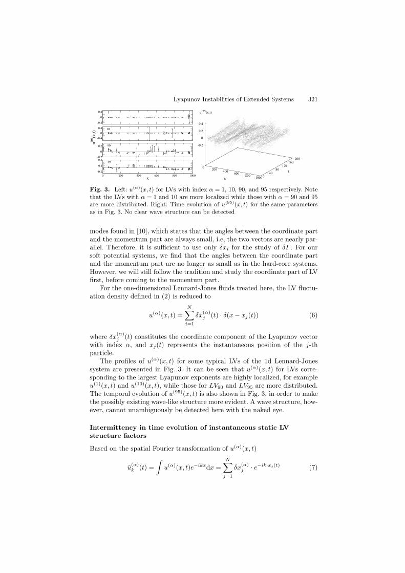
Lyapunov Instabilities of Extended Systems 321
-0.4
0
0.4
-0.4
0
0.4
-0.2
0
0.2
0 200 400 600 800 1000x
-0.2
0.1
0.4
u(α) (x
,t)
1
10
90
95
0200
400600
8001000x
040
80120
160200
t
-0.2
0
0.2
0.4
u(95)
(x,t)
Fig. 3. Left: u(α)(x, t) for LVs with index α = 1, 10, 90, and 95 respectively. Notethat the LVs with α = 1 and 10 are more localized while those with α = 90 and 95are more distributed. Right: Time evolution of u(95)(x, t) for the same parametersas in Fig. 3. No clear wave structure can be detected
modes found in [10], which states that the angles between the coordinate partand the momentum part are always small, i.e, the two vectors are nearly par-allel. Therefore, it is sufficient to use only δxi for the study of δΓ . For oursoft potential systems, we find that the angles between the coordinate partand the momentum part are no longer as small as in the hard-core systems.However, we will still follow the tradition and study the coordinate part of LVfirst, before coming to the momentum part.
For the one-dimensional Lennard-Jones fluids treated here, the LV fluctu-ation density defined in (2) is reduced to
u(α)(x, t) =
N∑
j=1
δx(α)j (t) · δ(x− xj(t)) (6)
where δx(α)j (t) constitutes the coordinate component of the Lyapunov vector
with index α, and xj(t) represents the instantaneous position of the j-thparticle.
The profiles of u(α)(x, t) for some typical LVs of the 1d Lennard-Jonessystem are presented in Fig. 3. It can be seen that u(α)(x, t) for LVs corre-sponding to the largest Lyapunov exponents are highly localized, for exampleu(1)(x, t) and u(10)(x, t), while those for LV90 and LV95 are more distributed.The temporal evolution of u(95)(x, t) is also shown in Fig. 3, in order to makethe possibly existing wave-like structure more evident. A wave structure, how-ever, cannot unambiguously be detected here with the naked eye.
Intermittency in time evolution of instantaneous static LVstructure factors
Based on the spatial Fourier transformation of u(α)(x, t)
u(α)k (t) =
∫u(α)(x, t)e−ikxdx =
N∑
j=1
δx(α)j · e−ik·xj(t) (7)
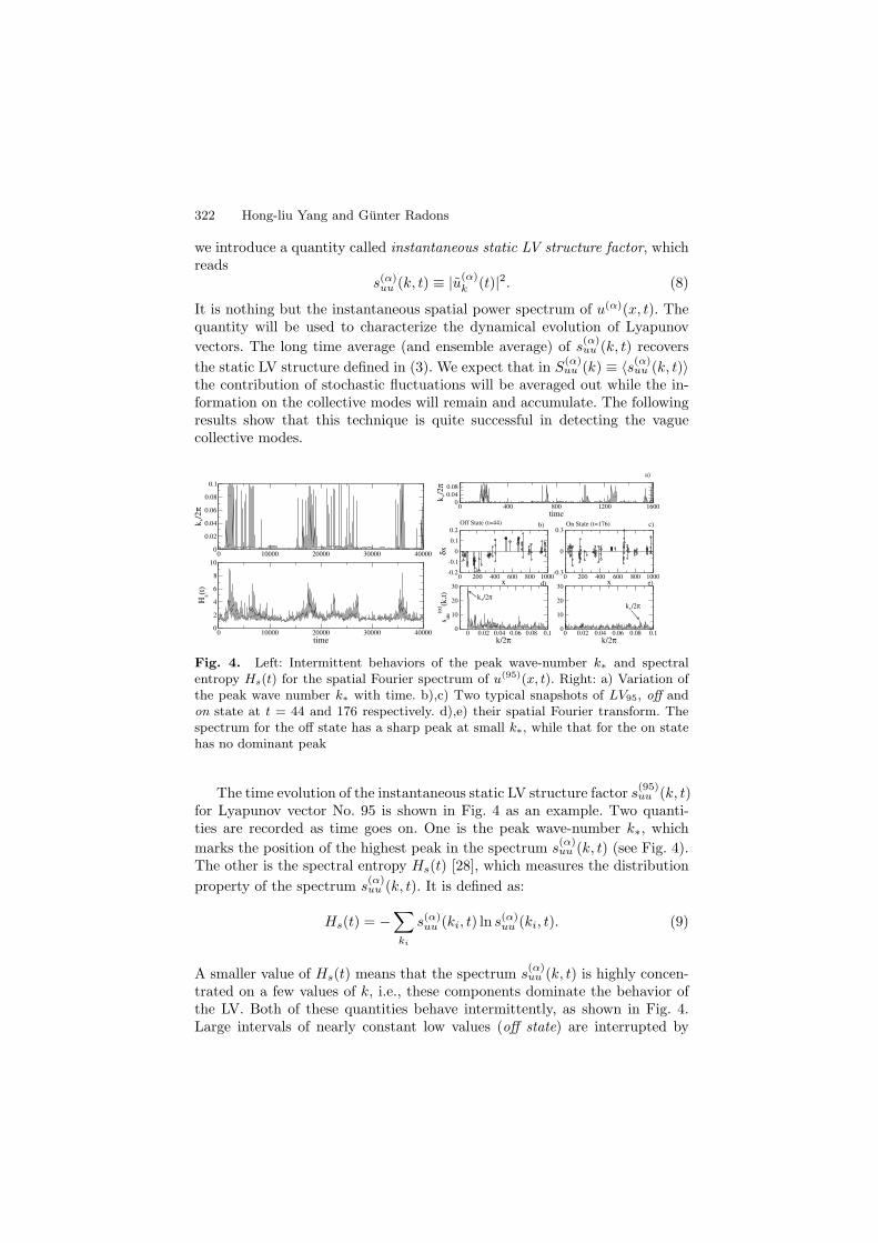
322 Hong-liu Yang and Gunter Radons
we introduce a quantity called instantaneous static LV structure factor, whichreads
s(α)uu (k, t) ≡ |u(α)
k (t)|2. (8)
It is nothing but the instantaneous spatial power spectrum of u(α)(x, t). Thequantity will be used to characterize the dynamical evolution of Lyapunov
vectors. The long time average (and ensemble average) of s(α)uu (k, t) recovers
the static LV structure defined in (3). We expect that in S(α)uu (k) ≡ 〈s(α)
uu (k, t)〉the contribution of stochastic fluctuations will be averaged out while the in-formation on the collective modes will remain and accumulate. The followingresults show that this technique is quite successful in detecting the vaguecollective modes.
0 10000 20000 30000 400000
0.02
0.04
0.06
0.08
0.1
k */2π
0 10000 20000 30000 40000time
0
2
4
6
8
10
Hs(t
)
0 200 400 600 800 1000x
-0.2
-0.1
0
0.1
0.2
δx
0 200 400 600 800 1000x
-0.3
0
0.3
0 0.02 0.04 0.06 0.08 0.1k/2π
0
10
20
30
s uu
(α) (k
,t)
0 0.02 0.04 0.06 0.08 0.1k/2π
0
10
20
30
0 400 800 1200 1600time
00.040.08
k */2π
Off State (t=44) On State (t=176)
k*/2π
k*/2π
a)
b) c)
d) e)
Fig. 4. Left: Intermittent behaviors of the peak wave-number k∗ and spectralentropy Hs(t) for the spatial Fourier spectrum of u(95)(x, t). Right: a) Variation ofthe peak wave number k∗ with time. b),c) Two typical snapshots of LV95, off andon state at t = 44 and 176 respectively. d),e) their spatial Fourier transform. Thespectrum for the off state has a sharp peak at small k∗, while that for the on statehas no dominant peak
The time evolution of the instantaneous static LV structure factor s(95)uu (k, t)
for Lyapunov vector No. 95 is shown in Fig. 4 as an example. Two quanti-ties are recorded as time goes on. One is the peak wave-number k∗, which
marks the position of the highest peak in the spectrum s(α)uu (k, t) (see Fig. 4).
The other is the spectral entropy Hs(t) [28], which measures the distribution
property of the spectrum s(α)uu (k, t). It is defined as:
Hs(t) = −∑
ki
s(α)uu (ki, t) ln s(α)
uu (ki, t). (9)
A smaller value of Hs(t) means that the spectrum s(α)uu (k, t) is highly concen-
trated on a few values of k, i.e., these components dominate the behavior ofthe LV. Both of these quantities behave intermittently, as shown in Fig. 4.Large intervals of nearly constant low values (off state) are interrupted by
Lyapunov Instabilities of Extended Systems 323
short period of bursts (on state) where they have large values. Details of typ-ical on and off states are shown in the right part of Fig. 4. One can see thatthe off state is dominated by low wave-number components (see the sharppeak at low wave-number k∗), while the on state is more noisy and there areno significant dominant components. This intermittency in the time evolutionof the instantaneous static LV structure factors is a typical feature of softpotential systems. It is conjectured that this is a consequence of the mixingof nearby LVs caused by the wild fluctuations of local instabilities. Due to themutual interaction among modes, the hydrodynamic Lyapunov modes in thesoft potential systems are only of finite life-time. In the dynamic Lyapunovstructure function estimated, the peak representing the propagating (or oscil-lating) Lyapunov modes is of finite width. This is support for our conjecturethat the hydrodynamic Lyapunov modes are of finite life-time.
Dispersion relation of hydrodynamic Lyapunov modes
Now, we consider the static LV structure factor S(α)uu (k), which is the long-time
average of the instantaneous quantity s(α)uu (k). Two cases with L = 1000 and
2000 are shown in Fig. 5. It is not hard to recognize the sharp peak at λ ≈ 0in the contour plot of the spectrum. With increasing Lyapunov exponents,the peak shifts to the larger wave number side. A dashed line is plotted tomake clear how the wave number of the peak kmax changes with λ(α). Tofurther demonstrate this point, the value of the Lyapunov exponent λ(α) isplotted versus kmax of corresponding LVs in Fig. 6. We call this the dispersionrelation of the hydrodynamical Lyapunov modes. The numerical fitting of thedata shows that for λ ≈ 0, λ(α) ∼ kγ
max with the exponent γ ≈ 1.2. Wepresume that a linear dispersion relation λ(α) ∼ kmax may be obtained as thethermodynamic limit is approached and the deviation from the linear functionof the data shown in Fig. 6 could be due to finite-size effects.
In order to show that the peak in S(α)uu (k) is not a result of the highly
regular packing of particles in the broken-chain state, the static structurefunction [25]
S(k) ≡∫G(r)e−ikrdr (10)
for the case L = 2000 is plotted in the same figure as S(α)uu (k), where G(r)
is the pair correlation function shown in Fig. 1. Obviously, S(k) is nearlyconstant in the regime k ≈ 0, the place where a sharp peak was observed in
S(α)uu (k). The regular packing of particles causes the formation of a peak atk/2π ≈ 0.9 in S(k). This corresponds to a tiny peak at the same k-value in
S(α)uu (k) for those LVs with λ ≈ 0. These facts show clearly that the collective
modes observed in the LVs are not caused by the regular packing of particles.
All of our results shown above provide strong evidence to the fact thatthe Lyapunov vectors corresponding to the smallest positive LEs in our 1d
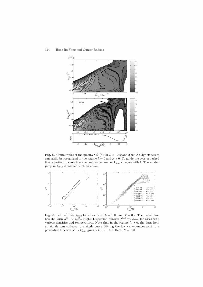
324 Hong-liu Yang and Gunter Radons
Fig. 5. Contour plot of the spectra S(α)uu (k) for L = 1000 and 2000. A ridge structure
can easily be recognized in the regime k ≈ 0 and λ ≈ 0. To guide the eyes, a dashedline is plotted to show how the peak wave-number kmax changes with λ. The suddenjump in kmax is marked with an arrow
10-4
10-3
10-2
10-1
100
kmax
(α)/2π
10-4
10-3
10-2
10-1
λ(α
)
10-4
10-3
10-2
10-1
100
kmax
/2π
10-4
10-3
10-2
10-1
λ(α
)
ρ=1/4 Τ=0.2ρ=1/6 Τ=0.2ρ=1/8 Τ=0.2ρ=1/10 Τ=0.2ρ=1/15 Τ=0.2ρ=1/20 Τ=0.2ρ=1/30 Τ=0.2ρ=1/40 Τ=0.2
ρ=1/4 Τ=0.3ρ=1/6 Τ=0.3ρ=1/8 Τ=0.3ρ=1/10 Τ=0.3ρ=1/4 Τ=0.4ρ=1/6 Τ=0.4ρ=1/8 Τ=0.4ρ=1/10 Τ=0.4
Fig. 6. Left: λ(α) vs. kmax for a case with L = 1000 and T = 0.2. The dashed linehas the form λ(α) ∼ k1.2
max. Right: Dispersion relation λ(α) vs. kmax for cases withvarious densities and temperatures. Note that in the regime λ ≈ 0, the data fromall simulations collapse to a single curve. Fitting the low wave-number part to apower-law function λα ∼ kγ
max gives γ ≈ 1.2 ± 0.1. Here, N = 100
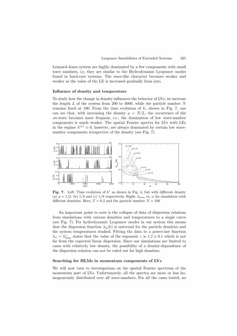
Lyapunov Instabilities of Extended Systems 325
Lennard-Jones system are highly dominated by a few components with smallwave numbers, i.e, they are similar to the Hydrodynamic Lyapunov modesfound in hard-core systems. The wave-like character becomes weaker andweaker as the value of the LE is increased gradually from zero.
Influence of density and temperature
To study how the change in density influences the behavior of LVs, we increasethe length L of the system from 200 to 4000, while the particle number Nremains fixed at 100. From the time evolution of k∗ shown in Fig. 7, onecan see that, with increasing the density ρ = N/L, the occurrence of theon-state becomes more frequent, i.e., the domination of low wave-numbercomponents is much weaker. The spatial Fourier spectra for LVs with LEsin the regime λ(α) ≃ 0, however, are always dominated by certain low wave-number components irrespective of the density (see Fig. 7).
0
0.2
0.4
0.6
k*/2
π
0
0.1
0.2
0.3
k */2
π
0 10000 20000 30000 40000time
0
0.05
0.1
0.15
k*/2
π
(a)
(b)
(c)
0 20 40 60 80 100α
0.0
0.1
0.2
0.3
km
ax/2
π
ρ=1/4ρ=1/6
ρ=1/2
ρ=1/8
ρ=1/10
ρ=1/15
ρ=1/20
Fig. 7. Left: Time evolution of k∗ as shown in Fig. 4, but with different density(a) ρ = 1/2, (b) 1/4 and (c) 1/8 respectively. Right: kmax vs. α for simulation withdifferent densities. Here, T = 0.2 and the particle number N = 100
An important point to note is the collapse of data of dispersion relationsfrom simulations with various densities and temperatures to a single curve(see Fig. 7). For hydrodynamic Lyapunov modes in our system this meansthat the dispersion function λα(k) is universal for the particle densities andthe system temperatures studied. Fitting the data to a power-law functionλα ∼ kγ
max states that the value of the exponent γ is 1.2 ± 0.1 which is notfar from the expected linear dispersion. Since our simulations are limited tocases with relatively low density, the possibility of a density-dependence ofthe dispersion relation can not be ruled out for high densities.
Searching for HLMs in momentum components of LVs
We will now turn to investigations on the spatial Fourier spectrum of themomentum part of LVs. Unfortunately, all the spectra are more or less ho-mogeneously distributed over all wave-numbers. For all the cases tested, no
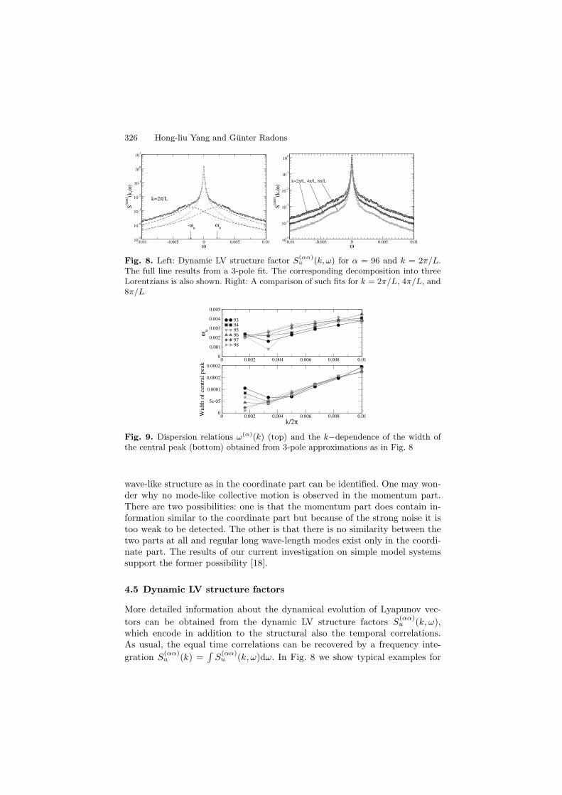
326 Hong-liu Yang and Gunter Radons
-0.01 -0.005 0 0.005 0.01ω
10-5
10-4
10-3
10-2
10-1
100
101
S(α
α) (k
,ω)
-ωu
ωu
k=2π/L
-0.01 -0.005 0 0.005 0.01ω
10-5
10-4
10-3
10-2
10-1
100
S(α
α) (k
,ω)
k=2π/L, 4π/L, 8π/L
Fig. 8. Left: Dynamic LV structure factor S(αα)u (k, ω) for α = 96 and k = 2π/L.
The full line results from a 3-pole fit. The corresponding decomposition into threeLorentzians is also shown. Right: A comparison of such fits for k = 2π/L, 4π/L, and8π/L
0 0.002 0.004 0.006 0.008 0.010
0.001
0.002
0.003
0.004
0.005
ωu
939495969798
0 0.002 0.004 0.006 0.008 0.01k/2π
0
5e-05
0.0001
0.0002
0.0002
Wid
th o
f ce
ntra
l pe
ak
Fig. 9. Dispersion relations ω(α)(k) (top) and the k−dependence of the width ofthe central peak (bottom) obtained from 3-pole approximations as in Fig. 8
wave-like structure as in the coordinate part can be identified. One may won-der why no mode-like collective motion is observed in the momentum part.There are two possibilities: one is that the momentum part does contain in-formation similar to the coordinate part but because of the strong noise it istoo weak to be detected. The other is that there is no similarity between thetwo parts at all and regular long wave-length modes exist only in the coordi-nate part. The results of our current investigation on simple model systemssupport the former possibility [18].
4.5 Dynamic LV structure factors
More detailed information about the dynamical evolution of Lyapunov vec-
tors can be obtained from the dynamic LV structure factors S(αα)u (k, ω),
which encode in addition to the structural also the temporal correlations.As usual, the equal time correlations can be recovered by a frequency inte-
gration S(αα)u (k) =
∫S
(αα)u (k, ω)dω. In Fig. 8 we show typical examples for
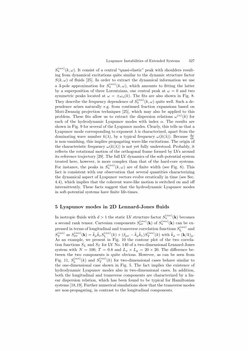
Lyapunov Instabilities of Extended Systems 327
S(αα)u (k, ω). It consist of a central “quasi-elastic” peak with shoulders result-
ing from dynamical excitations quite similar to the dynamic structure factorS(k, ω) of fluids [25]. In order to extract the dynamical information we use
a 3-pole approximation for S(αα)u (k, ω), which amounts to fitting the latter
by a superposition of three Lorentzians, one central peak at ω = 0 and twosymmetric peaks located at ω = ±ωu(k). The fits are also shown in Fig. 8.
They describe the frequency dependence of S(αα)u (k, ω) quite well. Such a de-
pendence arises naturally e.g. from continued fraction expansions based onMori-Zwanzig projection techniques [25], which may also be applied to thisproblem. These fits allow us to extract the dispersion relations ω(α)(k) foreach of the hydrodynamic Lyapunov modes with index α. The results areshown in Fig. 9 for several of the Lyapunov modes. Clearly, this tells us that aLyapunov mode corresponding to exponent λ is characterized, apart from thedominating wave number k(λ), by a typical frequency ω(k(λ)). Because dω
dkis non-vanishing, this implies propagating wave-like excitations. The origin ofthe characteristic frequency ω(k(λ)) is not yet fully understood. Probably, itreflects the rotational motion of the orthogonal frame formed by LVs aroundits reference trajectory [29]. The full LV dynamics of the soft-potential systemtreated here, however, is more complex than that of the hard-core systems.
For instance, the peaks in S(αα)u (k, ω) are of finite width (see Fig. 8). This
fact is consistent with our observation that several quantities characterizingthe dynamical aspect of Lyapunov vectors evolve erratically in time (see Sec.4.4), which implies that the coherent wave-like motion is switched on and offintermittently. These facts suggest that the hydrodynamic Lyapunov modesin soft-potential systems have finite life-times.
5 Lyapunov modes in 2D Lennard-Jones fluids
In isotropic fluids with d > 1 the static LV structure factor S(αα)u (k) becomes
a second rank tensor. Cartesian components S(αα)µν (k) of S
(αα)u (k) can be ex-
pressed in terms of longitudinal and transverse correlation functions S(αα)L and
S(αα)T as S
(αα)µν (k) = kµkνS
(αα)L (k) + (δµν − kµkν)S
(αα)T (k) with kµ = (k/k)µ.
As an example, we present in Fig. 10 the contour plot of the two correla-tion functions SL and ST for LV No. 140 of a two-dimensional Lennard-Jonessystem with N = 100, T = 0.8 and Lx × Ly = 20 × 20. The difference be-tween the two components is quite obvious. However, as can be seen from
Fig. 11, S(αα)L (k) and S
(αα)T (k) for two-dimensional cases behave similar to
the one-dimensional case shown in Fig. 5. The fact implies the existence ofhydrodynamic Lyapunov modes also in two-dimensional cases. In addition,both the longitudinal and transverse components are characterized by a lin-ear dispersion relation, which has been found to be typical for Hamiltoniansystems [18,19]. Further numerical simulations show that the transverse modesare non-propagating, in contrast to the longitudinal components.
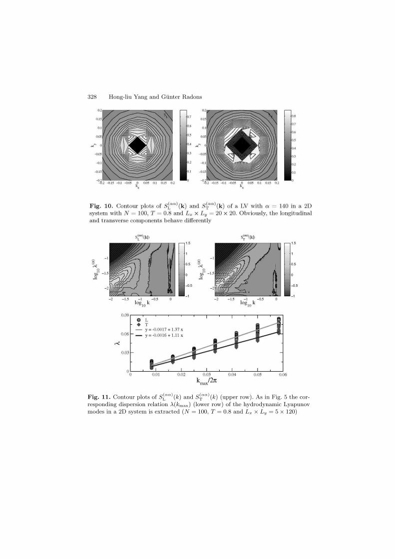
328 Hong-liu Yang and Gunter Radons
Fig. 11. Contour plots of S(αα)L (k) and S
(αα)T (k) (upper row). As in Fig. 5 the cor-
responding dispersion relation λ(kmax) (lower row) of the hydrodynamic Lyapunovmodes in a 2D system is extracted (N = 100, T = 0.8 and Lx × Ly = 5 × 120)

Lyapunov Instabilities of Extended Systems 329
6 Universal features of Lyapunov modes in spatiallyextended systems with continuous symmetries
Relying on the LV correlation function method, we have up to now successfullyidentified the existence of HLMs in the following spatially extended systems:
Coupled map lattices (CMLs) with either Hamiltonian or dissipative localdynamics
vlt+1 = (1− γ)vl
t + ǫ[f(ul+1t − ul
t)− f(ult − ul−1
t )] (11)
ult+1 = ul
t + vlt+1 (12)
andul
t+1 = ult + ǫ[f(ul+1
t − ult)− f(ul
t − ul−1t )] (13)
where f(z) is a nonlinear map, t is the discrete time index, l = 1, 2, · · · , Lis the index of the lattice sites and L is the system size. We set the dampingcoefficient γ = 0 and use periodic boundary conditions u0
t = uLt , u
L+1t = u1
t,unless it is explicitly stated otherwise.
Dynamic XY model [30] with the Hamiltonian
H =∑
i
θi + ǫ∑
ij
[1− cos(θj − θi)]. (14)
Kuramoto-Sivashinsky equation [31]
ht = −hxx − hxxxx − h2x. (15)
A common feature of these systems is that they all hold certain continuoussymmetries and conserved quantities, which have been shown to be essentialfor the occurrence of Lyapunov modes [18]. Our numerical simulations andanalytical calculations indicate that these systems fall into two groups withrespect to the nature of hydrodynamic Lyapunov modes. To be precise, thedispersion relations are characterized by λ ∼ k and λ ∼ k2 in Hamiltonianand dissipative systems respectively, as Fig. 12 indicates. Moreover, the HLMsin Hamiltonian systems are propagating, whereas those in dissipative systemsshow only diffusive motion. Examples of dynamic LV structure factors for twoCMLs are presented in the right row of Fig. 12. In a), each spectrum hastwo sharp symmetric side-peaks located at ±ωu. Furthermore, ωu ≃ ±cukfor k ≥ 2π/L. These facts suggest that the HLMs in coupled standard mapsare propagating. The spectrum of coupled circle maps in b) has only a singlecentral peak and can be well approximated by a Lorentzian curve [18], whichimplies that the HLMs in this system fluctuate diffusively. In addition, nostep structures in Lyapunov spectra have been found in contrast to the hard-core systems. The quantities characterizing the dynamical evolutions of LVsin these systems exhibit intermittent behaviors.
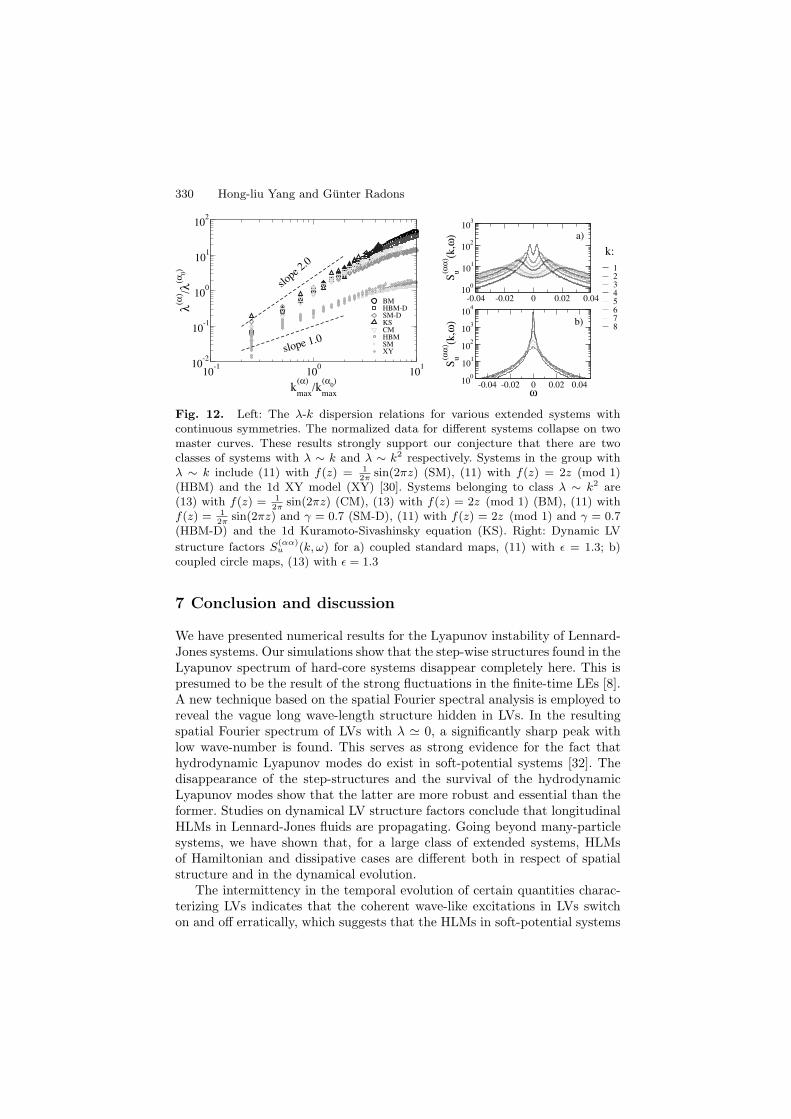
330 Hong-liu Yang and Gunter Radons
10-1
100
101
kmax
(α)/k
max
(α0)
10-2
10-1
100
101
102
λ(α
) /λ(α
0)
BMHBM-DSM-DKSCMHBMSMXY
slope 2
.0
slope 1.0
-0.04 -0.02 0 0.02 0.0410
0
101
102
103
Su(α
α) (k
,ω)
12345678
-0.04 -0.02 0 0.02 0.04ω
100
101
102
103
104
Su(α
α) (k
,ω)
a)
b)
k:
Fig. 12. Left: The λ-k dispersion relations for various extended systems withcontinuous symmetries. The normalized data for different systems collapse on twomaster curves. These results strongly support our conjecture that there are twoclasses of systems with λ ∼ k and λ ∼ k2 respectively. Systems in the group withλ ∼ k include (11) with f(z) = 1
2πsin(2πz) (SM), (11) with f(z) = 2z (mod 1)
(HBM) and the 1d XY model (XY) [30]. Systems belonging to class λ ∼ k2 are(13) with f(z) = 1
2πsin(2πz) (CM), (13) with f(z) = 2z (mod 1) (BM), (11) with
f(z) = 12π
sin(2πz) and γ = 0.7 (SM-D), (11) with f(z) = 2z (mod 1) and γ = 0.7(HBM-D) and the 1d Kuramoto-Sivashinsky equation (KS). Right: Dynamic LV
structure factors S(αα)u (k, ω) for a) coupled standard maps, (11) with ǫ = 1.3; b)
coupled circle maps, (13) with ǫ = 1.3
7 Conclusion and discussion
We have presented numerical results for the Lyapunov instability of Lennard-Jones systems. Our simulations show that the step-wise structures found in theLyapunov spectrum of hard-core systems disappear completely here. This ispresumed to be the result of the strong fluctuations in the finite-time LEs [8].A new technique based on the spatial Fourier spectral analysis is employed toreveal the vague long wave-length structure hidden in LVs. In the resultingspatial Fourier spectrum of LVs with λ ≃ 0, a significantly sharp peak withlow wave-number is found. This serves as strong evidence for the fact thathydrodynamic Lyapunov modes do exist in soft-potential systems [32]. Thedisappearance of the step-structures and the survival of the hydrodynamicLyapunov modes show that the latter are more robust and essential than theformer. Studies on dynamical LV structure factors conclude that longitudinalHLMs in Lennard-Jones fluids are propagating. Going beyond many-particlesystems, we have shown that, for a large class of extended systems, HLMsof Hamiltonian and dissipative cases are different both in respect of spatialstructure and in the dynamical evolution.
The intermittency in the temporal evolution of certain quantities charac-terizing LVs indicates that the coherent wave-like excitations in LVs switchon and off erratically, which suggests that the HLMs in soft-potential systems
Lyapunov Instabilities of Extended Systems 331
have finite life-times. This finding is consistent with the observation that indynamic LV structure factors the side-peaks representing the dynamical exci-tations have finite widths. This may also be related to the strong fluctuationsin the finite-time LEs.
Until now, only the coordinate part of LVs is used in most of the studieson hydrodynamic Lyapunov modes. For the case of hard-core systems, this isreasonable due to an interesting feature of those LVs corresponding to near-zero LEs found in [10], namely the fact that the angles between the coordinatepart and the momentum part are always small, i.e, the two vectors are nearlyparallel. For our soft potential systems, we find that the angles between thecoordinate part and the momentum part are no longer as small as in hard-coresystems. However, we failed to detect any long wave-length structures in themomentum part of LVs. This could be explained by our current results on thesimple model system of coupled map lattices (CMLs) [18].
The standard method of [20] was employed to calculate Lyapunov expo-nent and vectors quantities for our many-particle (N = 100− 1000) Lennard-Jones system in d dimension. A set of 2dN × 2dN linear and 2dN nonlinearordinary differential equations have to be integrated simultaneously in orderto obtain the dynamics of 2dN offset vectors in tangent space and the refer-ence trajectory in phase space, respectively. This enforces the use of parallelimplementations of the corresponding algorithms. Performance tests of ourparallel algorithms were executed on clusters with different hardware proper-ties. An efficient combination of basic routines and parallel orthogonalizationalgorithms make our exploration of the challenge field of Lyapunov instabili-ties of large dynamical systems feasible with the state art of computer powerand yields the reported interesting results.
Acknowledgments
We thank W. Just, W. Kob, A. Latz, A. S. Pikovsky and H. A. Posch forfruitful discussions. Special thanks go to W. Kob for providing us with thecode of molecular dynamics simulations and to G. Runger and M. Schwindfor the help on the parallel algorithms.
References
1. J.-P. Eckmann and D. Ruelle. Ergodic theory of chaos and strange attractors.Rev. Mod. Phys., 57:617, 1985; E. Ott. Chaos in Dynamical Systems. CambridgeUniversity Press, Cambridge, 1993.
2. N. S. Krylov. Works on the Foundations of Statistical Mechanics. PrincetonUniversity Press, Princeton, 1979.
3. P. Gaspard. Chaos, Scattering, and Statistical Mechanics. Cambridge UniversityPress, Cambridge, 1998.
4. J. P. Dorfman. An Introduction to Chaos in Nonequilibrium Statistical Mechan-ics. Cambridge University Press, Cambridge, 1999.
332 Hong-liu Yang and Gunter Radons
5. D. J. Evans and G. P. Morriss. Statistical Mechanics of Nonequilibrium Liquids.Academic, New York, 1990.
6. Wm. G. Hoover. Time Reversibility, Computer Simulation, and Chaos. WorldScientific, Singapore, 1999.
7. H. A. Posch and R. Hirschl. Simulation of blliards and of hard-body fluids. InD. Szasz, editor, Hard Ball Systems and the Lorenz Gas, Springer, Berlin, 2000.
8. C. Forster, R. Hirschl, H. A. Posch, and Wm. G. Hoover. Perturbed phase-spacedynamics of hard-disk fluids. Physics D, 187:294, 2004.
9. J.-P. Eckmann and O. Gat. Hydrodynamic Lyapunov modes in translation-invariant systems. J. Stat. Phys., 98:775, 2000.
10. S. McNamara and M. Mareschal. Origin of the hydrodynamic Lyapunov modes.Phys. Rev. E, 64:051103, 2001.
11. A. de Wijn and H. van Beijeren. Goldstone modes in Lyapunov spectra of hardsphere systems. Phys. Rev. E, 70:016207, 2004.
12. T. Taniguchi and G. P. Morriss. Stepwise structure of Lyapunov spectrafor many-particle systems using a random matrix dynamics. Phys. Rev. E,65:056202, 2002.
13. T. Taniguchi and G. P. Morriss. Boundary effects in the stepwise structure of theLyapunov spectra for quasi-one-dimensional systems. Phys. Rev. E, 68:026218,2003.
14. Wm. G. Hoover, H. A. Posch, C. Forster, C. Dellago and M. Zhou. Lyapunovmodes of two-Dimensional many-body systems; soft disks, hard disks, and rotors.J. Stat. Phys., 109:765, 2002.
15. H.-L. Yang and G. Radons. Lyapunov instabilities of Lennard-Jones fluids. Phys.Rev. E, 71:036211, 2005, see also arXiv:nlin.CD/0404027.
16. G. Radons and H.-L. Yang. Static and dynamic correlations in many-particleLyapunov vectors. arXiv:nlin.CD/0404028.
17. H.-L. Yang and G. Radons. Universal features of hydrodynamic Lyapunov modesin extended systems with continuous symmetries. Phys. Rev. Lett., 96:074101,2006.
18. H.-L. Yang and G. Radons. Hydrodynamic Lyapunov modes in coupled maplattices. Phys. Rev. E, 73:016202, 2006.
19. H.-L. Yang and G. Radons. Dynamical behavior of hydrodynamic Lyapunovmodes in coupled map lattices. Phys. Rev. E, 73:016208, 2006.
20. G. Benettin, L. Galgani and J. M. Strelcyn. Kolmogorov entropy and numericalexperiments. Phys. Rev. A, 14:2338, 1976.
21. I. Shimada and T. Nagashima. A numerical approach to ergodic problem ofdissipative dynamical systems. Prog. Theor. Phys., 61:1605, 1979.
22. J. Dongarra, J. Du Croz, I. Duff and S. Hammarling. A set of Level 3 BasicLinear Algebra Subprograms. ACM Trans. Math. Soft., 16:1, 1990.
23. L. S. Blackford, et al.. ScaLAPACK Users’ Guide. Society for Industrial andApplied Mathematics, Philadelphia, 1997.
24. G. Radons, G. Runger, M. Schwind and H.-L. Yang. Parallel algorithms for thedetermination of Lyapunov characteristics of large nonlinear dynamical systems.Proceedings of PARA04, WORKSHOP ON STATE-OF-THE-ART IN SCIEN-TIFIC COMPUTING, Lyngby, June 20-23, 2004, Lecture Notes of ComputerScience, vol. 3272, 1131, Springer, Berlin, 2005.
25. J. P. Boon and S. Yip. Molecular Hydrodynamics. McGraw-Hill, New York, 1980.
Lyapunov Instabilities of Extended Systems 333
26. W. Kob and H. C. Andersen. Testing mode-coupling theory for a supercooledbinary Lennard-Jones mixture I: The van Hove correlation function. Phys. Rev.E, 51:4626, 1995.
27. F. H. Stillinger. Statistical mechanics of metastable matter: superheated andstretched liquids. Phys. Rev. E, 52:4685, 1995.
28. R. Livi, M. Pettini, S. Ruffo, M. Sparpaglione and A. Vulpiani. Equipartitionthreshold in nonlinear large Hamiltonian systems: The Fermi-Pasta-Ulam model.Phys. Rev. A, 31:1039, 1985.
29. J.-P. Eckmann, C. Forster, H. A. Posch and E. Zabey. Lyapunov modes in hard-disk systems. J. Stat. Phys., 118:795, 2005.
30. D. Escande, H. Kantz, R. Livi and S. Ruffo. Self-consistent check of the valid-ity of Gibbs calculus using dynamical variables. J. Stat. Phys., 76:605, 1994;M. Antoni and S. Ruffo. Clustering and relaxation in Hamiltonian long-rangedynamics. Phys. Rev. E, 52:2361, 1995.
31. Y. Kuramoto and T. Tsuzuki. Persistent propagation of concentration wavesin dissipative media far from thermal equilibrium. Prog. Theor. Phys., 55:356,1976; G. I. Sivashinsky. Acta Astron., 4:1177, 1977.
32. C. Forster and H. A. Posch. Lyapunov modes in soft-disk fluids. New J. Phys.,7:32, 2005, see also arXiv:nlin.CD/0409019

The Cumulant Method for Gas Dynamics
Steffen Seeger1, Karl Heinz Hoffmann2, and Arnd Meyer3
1 [email protected] Technische Universitat Chemnitz, Institut fur Physik
09107 Chemnitz, [email protected]
3 Technische Universitat Chemnitz, Fakultat fur Mathematik09107 Chemnitz, [email protected]
1 Introduction
Characterizing fluid flow by the ratio of mean free path and a characteristicflow length (the Knudsen number Kn) we have two extremes: dense gases(Kn ≪ 1) where modeling by Euler or Navier-Stokes equations is validand rarefied gases (Kn ≫ 1) for which modeling by the Boltzmann equa-tion is necessary. Developing models for the intermediate transition regime issubject to active current research because despite the tremendously growingincrease in computational and algorithmic computing performance, numericalsimulation of flows in the transition regime remains a challenging problem.Thus there is a considerable gap in the ability to model flows where meanfree path and characteristic flow lengths are comparable. However, efficientmethods for simulating transition regime flows will be an important designtool for micro-scale machinery, where dense gas models become invalid.
As can be learned from the tremendous advances of computational meth-ods for the Navier-Stokes equations, an important key for the efficient solu-tion is the use of (structured) adaptivity and parallel methods of solution. Foran efficient parallel implementation with good speedup, the resulting numer-ical scheme should require only local operations and require only moderatecommunication. Adaptivity, however, has so far mainly been used for grid re-finement to achieve the accuracy goals for numerical solution. To obtain thenecessary gain in efficiency for the transition regime flows, it seems naturalto extend the concept of adaptivity also to physical modelling (that is, the‘detail’ of the equations of motion to be solved in a certain flow regime). Thisrequires a consistent theory of how these equations are related to each other,and how the coupling could be achieved consistently.
The derivation of reduced, but nevertheless consistent equations of motionfor fluid flow is therefore an interesting question of current research. The goal is

336 Steffen Seeger et al.
do develop a description of fluid flow which can be adjusted in detail betweenthat of the Boltzmann equation and that of Euler equations. Here wepresent some results from our work on physical models for these flows, tryingto shed more light on the question how properly chosen physical models mightallow for such adaptivity not only in numerical solution but also in physicalmodelling.
Two schemes that try to successively approximate the Boltzmann equa-tion to include more and more detail are moment methods [1–3] and thecumulant method [4–6]. Commonly a rather small number of moments or cu-mulants is used and thus these methods do not capture the full informationavailable with the phase space density, but focus on physically interestingmacroscopic quantities, such as density, flow velocity, mean kinetic energy,shear stress and heat flux.
This work is intended to give a review of the theory and results for the cu-mulant method, in order to serve as a starting point for the interested reader.The first part of the review gives a short introduction to kinetic theory, namelythe Boltzmann equation, the interaction model, and the space-homogeneouscase. The second part discusses the basic concepts and differences of the var-ious moment methods known from the literature. The last part presents thecumulant method, results on properties of the resulting equations, a simplenumerical scheme to solve them and possible boundary conditions. A summaryand outlook to possible future research closes this review.
2 Kinetic theory
Considering flow of an inert mixture of gases we assume the fluid is composedof Ns different species, enumerated by the set Ns with each species having itsown set of associated properties. For a species s, these are the particle massms and the laws of interaction with particles of any other species r. We let thephase space density fs(t, x, cs) denote the density of particles of species s attime t and position x, moving with absolute velocity c. The fs are normalizedsuch that
ns(t, x) =
∫dc fs(t, x, c) (1)
are the partial particle number densities of the various species (integrals aretaken over the whole velocity space Rd).
2.1 The Boltzmann equation
The fs have to satisfy the Boltzmann equation. Considering a sufficientlydilute gas in an inertial frame, where accounting only for binary collisions issufficient, this integro-differential equation in the fs takes the form [7]
∂t fs + c · ∂x fs + as · ∂c fs =∑
r∈Ns
Srs[fr, fs] ; ∀s ∈ Ns (2)
The Cumulant Method for Gas Dynamics 337
where Srs denotes the collision operator and as denotes the acceleration ofa s-particle due to external forces as a function of time t, particle position xand particle velocity c. We regard forces exerted on particles due to particle-particle interaction as internal and any other (e.g. gravity) as external. Thefunctional Srs[fr, fs] occurring in equation (2) describes the change of fs dueto interaction of particles of species r with particles of species s. By restric-tion to the description of a sufficiently dilute gas it may be assumed that: I)contributions by other than binary collisions may be neglected; II) the rangeof interaction is much less than the mean free path; III) particle trajectoriesbefore and after the collision are approximately rectilinear; IV) the distribu-tion functions are constant over the range of interaction; V) particles aboutto collide are not correlated. With these assumptions Srs can be written asthe integral operator
Srs[fr, fs] =∑
r
∫dcr dn σrs ‖crs‖ (frfs − frfs) (3)
with scattering cross section σrs = σrs(n, ‖crs‖), relative collision velocitycrs = cr−cs, ‖crs‖ =
√crs · crs denoting the usual quadratic vector norm and
the collision parameter vector n. The integral over dn covers the d-dimensionalsphere ‖n‖ = 1. fr and fs are the phase-space densities evaluated at thevelocities cr and cs after the collision.
For a gas at standard conditions, these assumptions are justified: witha typical molecule diameter of about 0.3 nm and a particle density of n ≈2.7 · 1025 m−3 the average distance of the particles is about ten times themolecule diameter, making the first assumption hold. The mean free path is≈ 10 nm, so it is about 10 times longer than the range of interaction, whichmakes the second assumption reasonable. This allows to abstract from the par-ticular particle trajectories during an encounter to states ‘before’ and ‘after’a collision. With intermolecular forces generally several powers of ten largerthan external forces (e.g. gravity) the third assumption allows to neglect theeffect of external forces during a collision. The fourth assumption is certainlyvalid if there are no steep gradients in density or kinetic temperature. The lastassumption does not have any obvious justification but is postulated to holdfor dilute gases (where particles participating in a collision stem from regions afew mean free path lengths apart), but it is supported by excellent agreementof the results of kinetic theory of dilute gases with known experiments.
2.2 The Enskog equation of change
Describing the evolution of mixtures of gases on a macroscopic scale we areinterested in partial quantities, such as the partial pressure, density, etc. ofeach species. Given a phase space density fs(t, x, c), the density of a partialmacroscopic thermodynamic quantity (Φ)s(t, x) can be obtained as the meanof an associated microscopic function Φ(t, x, c)
338 Steffen Seeger et al.
(Φ)s(t, x) =
∫dc Φ(t, x, c) fs(t, x, c) . (4)
Multiplying (2) with Φ and integrating over c we obtain [8] a balance equationfor the quantity (Φ)s (also known as Enskog’s general equation of change)
∂t (Φ)s + ∂x · (c Φ)s =(∂tΦ + ∂x · cΦ + ∂c · asΦ
)s+
∑
r∈Ns
∫dc Φ Srs , (5)
where we made use of partial integration and the property fs → 0 for ‖c‖ → ∞due to (1).
2.3 The Maxwell gas model
Throughout this work we will assume the particular interaction model of so-called Maxwell molecules, for which the particles repel each other with aforce inversely proportional to the (2d − 1)th power of their distance. Ashas been known for quite a long time [9], this simplifies the collision integralconsiderably. Since the Boltzmann-type collision operator (3) is similar toa convolution integral, the simplifications are even greater when employinga Fourier-transformation with regard to particle velocity. This method oftransformation of the Boltzmann equation into an equation for the charac-teristic function [10] has been proposed and extensively studied by Bobylev
et al. [11] with a review of the method and results given in [12]. It can beapplied also for other interaction models (i.e. hard spheres and the BGK ap-proximation) but here we restrict our considerations to Maxwell interaction.
Setting Φ = 1(2 π)d/2 e
iχ·c we find the associated (Φ)s to be the character-
istic function ϕs(t, x, χ) with the equation of motion
∂tϕs + ∂x · ∂iχ ϕs = Γs +∑
r∈Ns
Ξrs[ϕr, ϕs] ,
collision term Ξrs[ϕr, ϕs] = 1(2π)d/2
∫dc Srs e
iχ·c
and force term Γs[ϕs] = 1(2 π)d/2
∫dc fs ∂c · as e
iχ·c .
(6)
After a straightforward calculation following the idea of Bobylev [11] we find
Ξ2Drs [ϕr, ϕs] =
√2 κrs
µrs(2π)2
∫dε Ω[ϕr, ϕs]
Ξ3Drs [ϕr, ϕs] =
√2 κrs
µrs(2π)3
∫dεdϕ εΩ[ϕr, ϕs]
(7)
for the 2D and 3D Maxwell gas respectively. Here ε is a dimensionless col-lision parameter, ϕ (without any index) is the tilt of the scattering plane and
The Cumulant Method for Gas Dynamics 339
κrs is the parameter controlling the strength of interaction between particlesof species r and s. The integral kernel Ω[ϕr, ϕs] is given by
Ω[ϕr, ϕs] = ϕr(χ · D+
+)ϕs(χ · D−
+)− ϕr(0)ϕs(χ) (8)
with
D+
+=[1+∆rs
2 1− 1+∆rs
2 S−1]
D−+
=[1−∆rs
2 1 + 1+∆rs
2 S−1], (9)
where S−1 denotes the inverse of the scattering matrix S that rotates crs tocrs. Note that this choice is a bit different from the common notation in kinetictheory, where the mapping from crs to crs is chosen as an unitary, symmetricmatrix. The common notation makes the mapping between crs and crs self-inverse, but here we prefer the given notation for easier calculation of theintegrals occurring in the production terms. ∆rs and µrs are calculated frommr and ms, the masses of r- and s-particles, as
µrs =mrms
mr +ms∆rs =
mr −ms
mr +ms. (10)
From the actual kinematics of a collision we find in 2D
ϑ2D(ε) = π
(1− ε√
1 + ε2
)and S(ε) =
cosϑ(ε) − sinϑ(ε)
sinϑ(ε) cosϑ(ε)
. (11)
with the collision angle ϑ given as a function of the dimensionless collisionparameter ε.
For convenient numerical implementation we use a system of units suchthat the relations and equations given remain unchanged but with kB = 1and the atomic mass unit mu = 1. That is, choosing a reference temperature,pressure and volume as that of 1mol of an ideal gas at the ice point of waterand using the atomic mass as unit for particle masses, we have determined theunits for length, time, energy etc. by the condition kB = 1. We can establishsuch a system of units for the 2D-case considered here as well and give anynumerical results, plots etc. in dimensionless form.
2.4 Spatially homogeneous Boltzmann equation
Let us now examine the spatially homogeneous case [13] for equation (2).All points x in space are assumed equal, so fs(t, x, c) does not depend on xand further the effect of external forces is neglected (a = 0). Thus we areconcerned with the temporal relaxation of a set of Ns phase space densitiesfs(t, ·, c) : R+ × Rd → R+ from initial non-equilibrium densities fs(0, ·, c)to equilibrium densities f eq
s (c) = f(∞, ·, c). According to (2) and (6), thisrelaxation is determined by the equation
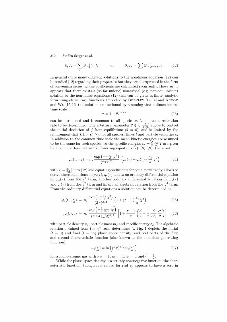
340 Steffen Seeger et al.
∂t fs =∑
r
Srs[fr, fs] or ∂tϕs =∑
r
Ξrs[ϕr, ϕs] . (12)
In general quite many different solutions to the non-linear equation (12) canbe studied [12] regarding their properties but they are all expressed in the formof converging series, whose coefficients are calculated recurrently. However, itappears that there exists a (so far unique) non-trivial (e.g. non-equilibrium)solution to the non-linear equations (12) that can be given in finite, analyticform using elementary functions. Reported by Bobylev [12,14] and Krook
and Wu [15,16] this solution can be found by assuming that a dimensionlesstime scale
τ = 1− θ e−λ t (13)
can be introduced and is common to all species s. λ denotes a relaxationrate to be determined. The arbitrary parameter θ ∈ [0, 2
d+2 ] allows to controlthe initial deviation of f from equilibrium (θ = 0), and is limited by therequirement that fs(t, ·, c) ≥ 0 for all species, times t and particle velocities c.In addition to the common time scale the mean kinetic energies are assumedto be the same for each species, so the specific energies εs = d
2kB
msT are given
by a common temperature T. Inserting equations (7), (8), (9), the ansatz
ϕs(t, ·, χ) = ns
exp(−τ εs
d χ2)
(2π)d/2
(ps(τ) + qs(τ) τ
εsdχ2)
(14)
with χ = ‖χ‖ into (12) and equating coefficients for equal powers of χ allows toderive three conditions on ps(τ), qs(τ) and λ: an ordinary differential equationfor ps(τ) from the χ0 term; another ordinary differential equation for ps(τ)
and qs(τ) from the χ2 term and finally an algebraic relation from the χ4 term.From the ordinary differential equations a solution can be determined as
ϕs(t, ·, χ) = ns
exp(−τ εs
d χ2)
(2π)d/2
(1 + (τ − 1)
εsdχ2)
(15)
fs(t, ·, c) = ns
exp(− 1
τd
2 εs
c2
2
)
(π τ 4 εs/d)d/2
[1 +
τ − 1
τ
(d
2− 1
τ
d
2 εs
c2
2
)](16)
with particle density ns, particle massms and specific energy εs. The algebraicrelation obtained from the χ4 term determines λ. Fig. 1 depicts the initial(t = 0) and final (t = ∞) phase space density, and real parts of the firstand second characteristic function (also known as the cumulant generatingfunction)
κs(χ) = ln((2π)d/2 ϕs(χ)
)(17)
for a mono-atomic gas with κ11 = 1, m1 = 1, ε1 = 1 and θ = 12 .
While the phase-space-density is a strictly non-negative function, the char-acteristic function, though real-valued for real χ, appears to have a zero in

The Cumulant Method for Gas Dynamics 341
-4 -2 0 2 4
0.0
0.1
0.2
0.0
0.1
0.2
-4 -2 0 2 4
-5
0
f(c)
φ(χ)
κ(χ)
Fig. 1. Radial cross sections of the initial (dashed) and final (solid) phase spacedensity (top), the characteristic function (center) and the real part of the secondcharacteristic function (bottom) for the 2D case. The phase space density is non-negative, the characteristic function, however, has two zeros which move to larger χwith time. These zeros result in two poles for the second characteristic function anda non-continuous imaginary part
the radial part, which results in a singularity for the real part and a non-continuous, but piecewise constant imaginary part of the cumulant generat-ing function (we restrict our considerations to the main branch of ln). Withtime advancing, the zero moves toward larger χ converging to the equilibriumsolution.
In the following we will restrict our considerations to the 2D-case, for whichwe obtain
λ =∑
r
nr
√2κrs
µrs
1−∆rs2
2
ω2 −∆rs2 (ω2 − 4ω1)
4(18)
where the ωn are constants given by
ωn =
+∞∫
−∞
dε 1− cos(nϑ2D(ε)
). (19)
In general relation (18) is not satisfied for all species s if we allow for anarbitrary choice of the species parameters µrs, ∆rs and κrs. Thus it shouldbe read as one rule for determination of λ and (Ns − 1) constraints on thespecies parameters.
342 Steffen Seeger et al.
3 Mesoscopic fluid modelling
For simulating transition regime flows it becomes essential to extend the wellknown macroscopic models to include a more detailed description of the fluidflow. This is because models for rather dense gases, such as the Euler orNavier-Stokes equations become invalid and methods of solving the Boltz-
mann equation become too expensive in this regime. Such flow conditions aremainly characterized by the mean free path being in the order of a characteris-tic flow length. Thus the flow conditions for the transition regime are betweendense gases (Kn ≪ 1) where modeling by Euler or Navier-Stokes equa-tions is valid and rarefied gases (Kn≫ 1) for which the Boltzmann equationis an adequate description.
3.1 Moment equations
By repeated differentiation of (6) with regard to χ and setting χ = 0 after-wards we find an infinite system of coupled, nonlinear balance equations
∂tM0s + ∂x ·M1
s = G0s +
∑r P
0rs
∂tM1s + ∂x ·M2
s = G1s +
∑r P
1rs
...
∂tMαs + ∂x ·Mα+1
s = Gαs +
∑r P
αrs
...
with
Mαs = (2π)d/2 ∂α
iχ ϕs
∣∣∣χ=0
Gαs = (2π)d/2 ∂α
iχ Γs
∣∣∣χ=0
Pαrs = (2π)d/2 ∂α
iχ Ξrs
∣∣∣χ=0
(20)for the so-called moments Mα
s = (cα)s. For powers of the particle velocity cor the partial derivative ∂iχ with respect to imaginary unit i times inverse
velocity χ a scalar exponent α denotes the tensorial power of order α, while amulti-index will denote the appropriate element of such a tensor. Similarly, forthe moments Mα
s , force terms Gαs and productions Pα
rs, a scalar superscriptα denotes the full tensor (of rank α) and a multi-index the correspondingelement.
Moments have been of particular interest, because the low order momentsare related to particle number density, momentum and energy density, all ofwhich are conserved quantities. And further, if one assumes the phasespacedensity fs describes a local equilibrium state (where equilibrium parametersmay vary with t and x), the low order moment equations give actually theEuler equations.
The advection term for equation α couples moments of order α and α+1, asthe flux in one equation appears as density in the equation of next higher orderand vice versa. In general we must assume that production terms may couplebetween any orders α, but for the particular interaction model considered herewe observe only coupling towards lower orders. Currently it appears to be not
The Cumulant Method for Gas Dynamics 343
even known whether the quantities appearing in equation (20) are well-definedfunctions for every solution of (2). E.g. boundedness of the appearing integralsor proper differentiability of the moments are by no means obvious for non-equilibrium solutions. Anyhow, moments have been shown to be well-definedat least for the spatially homogeneous [17] and the nearly homogeneous [18]case, so it might be more generally true.
3.2 The closure problem
One promising approach to modelling mesoscopic fluid flow is to consider finitesubsets of (20) as approximations of (2) by taking only equations of orderα = 0, . . . , Nα, where the ‘level of detail’ can be adjusted by Nα. Truncationof (20) at some order Nα imposes the so-called closure problem, which consistsin expressing the moments Mα
s , the force terms Gαs and the productions Pα
s
as a function of some set of variables (traditionally the moments themselves)so that the finite subsystem is closed. This is achieved by making an ansatz –or imposing physical principles to determine a suitable ansatz – for the phasespace density fs or the characteristic function ϕs with some ansatz parameters.Given the functional form of the ansatz, a relation of the parameters and themoments is determined by the condition that the first Nα moments of theansatz should equal those of the ‘true’ (but unknown) solution. Solving thisrelation for the parameters as a function of the moments allows to express theansatz for fs in terms of the moments and in turn to determine MNα+1
s , Gαs
and Pαs as a function of the moments so that (20) is closed.
There are various criteria proposed in the literature on how to achievethis closure. It turns out that moment method(s), regardless of the particularclosure employed, give results in good agreement with kinetic theory [19–22], where phenomenological descriptions of gases (like Navier-Stokes) fail.Nevertheless equations (20) are in general hard to obtain – even for statesclose to equilibrium – and become quickly very complicated with increasingorder Nα. In the following we give a short overview of the most importantproposals. There are more closure procedures discussed in the literature (see,for instance [23], [24]) but for the scope of this work we would like to restrictto the following approaches which are conceptually different.
In the method proposed by Grad [1], fs is factored into a (local) equi-librium part and a non-equilibrium part, the latter being expanded in a se-ries of Hermite polynomials ortho-normalized with regard to the (t, x)-localequilibrium part as weight function. From a slightly different point view, themethod of Grad may be viewed as an expansion of the phase space den-sity in terms of Hermite functions. As the Hermite functions, however, arethe eigenfunctions of the Fourier-transform this means that we may as wellview Grad’s approach as an expansion of the first characteristic function interms of Hermite-functions. Truncating the expansion at some arbitrary or-der Nα, this approach allows to determine the closure exactly but it appears
344 Steffen Seeger et al.
to be difficult to give useful expressions for the entropy density, its flux orproduction rate.
Waldmann [25] observed that – for states close to thermal equilibriumwhere a linear approximation of the collision operator holds – expressing fsas a sum of a (local) equilibrium and a small deviation-from-equilibrium partleads to a linear integro-differential equation for the deviation from equilib-rium. Assuming a space-homogeneous gas with a solution where the deviationfrom equilibrium decays exponentially in time leads to an eigenvalue prob-lem for the function describing the deviation from equilibrium. An analyticalsolution can be given for the special case of a Maxwell gas where an ortho-normal system of eigenfunctions can be constructed as a product of Sonine
polynomials and spherical harmonics when using spherical coordinates in ve-locity space. These correspond to irreducible homogeneous tensors when usingcartesian coordinates in velocity space, which is why Waldmann considersan expansion of the deviation from equilibrium with regard to these eigen-tensors of the linearized collision operator. Similar to Grad’s method, exactexpressions for the entropy density, it’s flux or production rate are difficult toobtain.
Existence of a properly defined entropy density is, however, the main em-phasis in the framework of Extended Irreversible Thermodynamics (EIT) byMueller et al. [2]. There a particular ansatz form is obtained by applying alocal formulation of the second law of thermodynamics. Unfortunately, closureis a very hard problem, as the ansatz function is an exponential of a tensorpolynomial in c. Nevertheless entropy density and flux can be given but itappears to be difficult to give an analytic form of the entropy production.Usually one resorts to an expansion of the exponential close to equilibrium,which leads to a closure similar to the one by Grad [26].
The entropy production is payed more attention to by the modified mo-ment method [27] proposed by Eu, where it is regarded a direct measure ofenergy dissipation. So the ansatz for fs is chosen such that the entropy produc-tion takes a simple form, making the connection of evolution of non-conservedvariables and entropy production quite obvious. But again: neither is therea method for exact closure nor is it simple to give an analytic form of theentropy density.
4 The cumulant method
For the cumulant method we make a Taylor expansion of the logarithm ofthe characteristic function, which simplifies the deriviation of the equationssatisfied by the ansatz parameters. The resulting equations are considerablysimpler than the equations obtained by the Method of Grad, however, itbecomes difficult to give an equivalent procedure of expansion for the phasespace density. We find the low order Grad coefficients to be equivalent tothe cumulants [4], but there are additional nonlinear terms in the relation
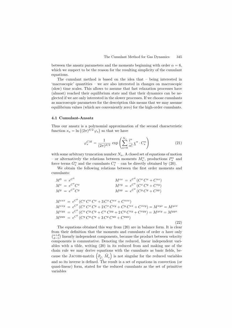
The Cumulant Method for Gas Dynamics 345
between the ansatz parameters and the moments beginning with order α = 6,which we suspect to be the reason for the resulting simplicity of the cumulantequations.
The cumulant method is based on the idea that – being interested in‘macroscopic’ quantities – we are also interested in changes on macroscopic(slow) time scales. This allows to assume that fast relaxation processes have(almost) reached their equilibrium state and that their dynamics can be ne-glected if we are only interested in the slower processes. If we choose cumulantsas macroscopic parameters for the description this means that we may assumeequilibrium values (which are conveniently zero) for the high-order cumulants.
4.1 Cumulant-Ansatz
Thus our ansatz is a polynomial approximation of the second characteristicfunction κs = ln
((2π)d/2 ϕs
)so that we have
ϕCMs =
1
(2π)d/2exp
(Nα∑
α=0
iα
α!χα · Cα
s
)(21)
with some arbitrary truncation numberNα. A closed set of equations of motion– or alternatively the relations between moments Mα
s , productions Pαs and
force terms Gαs and the cumulants Cα
s – can be directly obtained by (20).We obtain the following relations between the first order moments and
cumulants:
M0 = eC0
Mx = eC0
Cx
My = eC0
Cy
Mxx = eC0
(Cx Cx + Cxx)
Mxy = eC0
(Cx Cy + Cxy)
Myy = eC0
(Cy Cy + Cyy)
Mxxx = eC0
(Cx Cx Cx + 3Cx Cxx + Cxxx)
Mxxy = eC0
(Cx Cx Cy + 2Cx Cxy + Cy Cxx + Cxxy) =Mxyx =Myxx
Mxyy = eC0
(Cx Cy Cy + Cx Cyy + 2Cy Cxy + Cxyy) =Myxy =Myyx
Myyy = eC0
(Cy Cy Cy + 3Cy Cyy + Cyyy)(22)
The equations obtained this way from (20) are in balance form. It is clearfrom their definition that the moments and cumulants of order α have only(α+dd−1
)linearly independent components, because the product between velocity
components is commutative. Denoting the reduced, linear independent vari-ables with a tilde, writing (20) in its reduced from and making use of thechain rule we may derive equations with the cumulants as basic fields, be-
cause the Jacobi-matrix(∂
Cs
Ms
)is not singular for the reduced variables
and so its inverse is defined. The result is a set of equations in convection (orquasi-linear) form, stated for the reduced cumulants as the set of primitivevariables
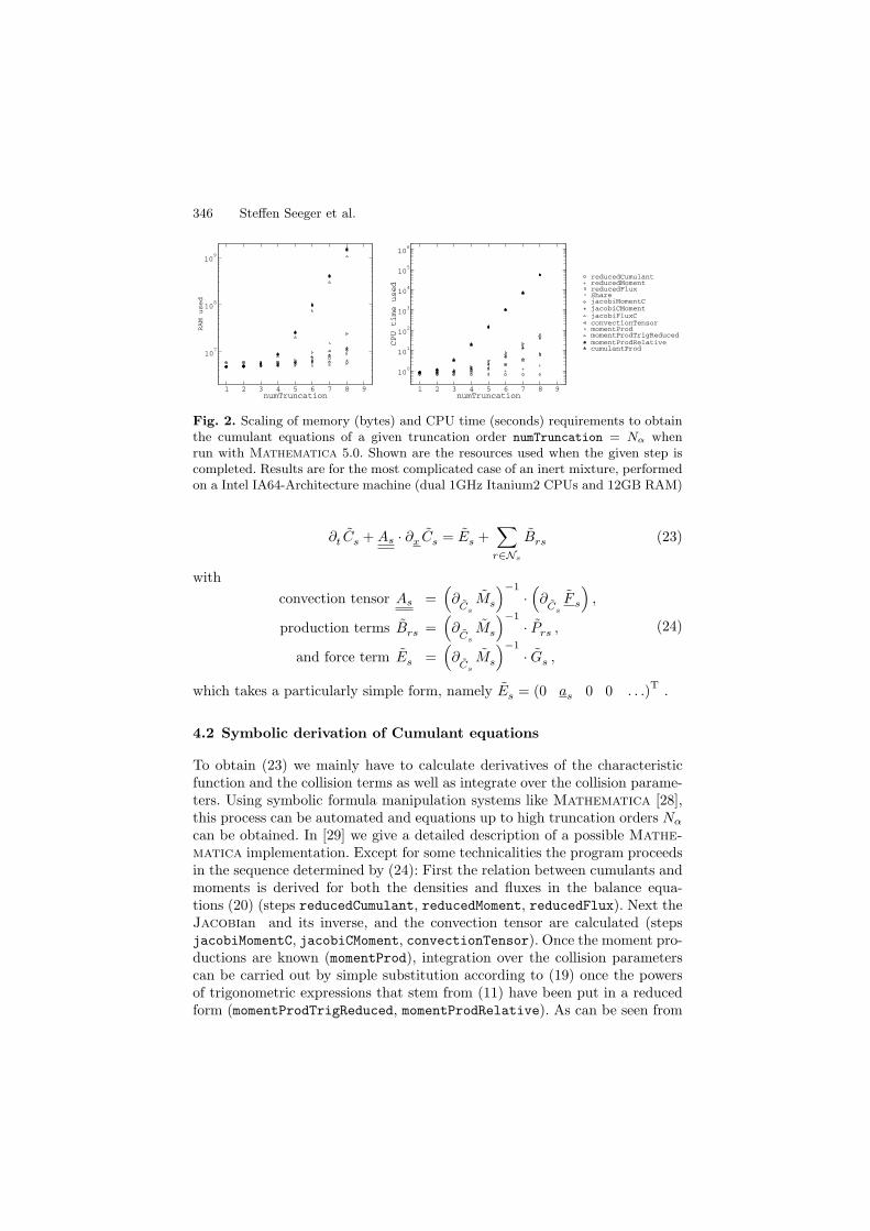
346 Steffen Seeger et al.
1 2 3 4 5 6 7 8 9numTruncation
107
108
109
RAM used
1 2 3 4 5 6 7 8 9numTruncation
100
101
102
103
104
105
106
CPU time used
reducedCumulantreducedMomentreducedFluxSharejacobiMomentCjacobiCMomentjacobiFluxCconvectionTensormomentProdmomentProdTrigReducedmomentProdRelativecumulantProd
Fig. 2. Scaling of memory (bytes) and CPU time (seconds) requirements to obtainthe cumulant equations of a given truncation order numTruncation = Nα whenrun with Mathematica 5.0. Shown are the resources used when the given step iscompleted. Results are for the most complicated case of an inert mixture, performedon a Intel IA64-Architecture machine (dual 1GHz Itanium2 CPUs and 12GB RAM)
∂t Cs +As · ∂x Cs = Es +∑
r∈Ns
Brs (23)
with
convection tensor As =(∂
Cs
Ms
)−1
·(∂
Cs
F s
),
production terms Brs =(∂
Cs
Ms
)−1
· Prs ,
and force term Es =(∂
Cs
Ms
)−1
· Gs ,
(24)
which takes a particularly simple form, namely Es = (0 as 0 0 . . .)T.
4.2 Symbolic derivation of Cumulant equations
To obtain (23) we mainly have to calculate derivatives of the characteristicfunction and the collision terms as well as integrate over the collision parame-ters. Using symbolic formula manipulation systems like Mathematica [28],this process can be automated and equations up to high truncation orders Nα
can be obtained. In [29] we give a detailed description of a possible Mathe-
matica implementation. Except for some technicalities the program proceedsin the sequence determined by (24): First the relation between cumulants andmoments is derived for both the densities and fluxes in the balance equa-tions (20) (steps reducedCumulant, reducedMoment, reducedFlux). Next theJacobian and its inverse, and the convection tensor are calculated (stepsjacobiMomentC, jacobiCMoment, convectionTensor). Once the moment pro-ductions are known (momentProd), integration over the collision parameterscan be carried out by simple substitution according to (19) once the powersof trigonometric expressions that stem from (11) have been put in a reducedform (momentProdTrigReduced, momentProdRelative). As can be seen from
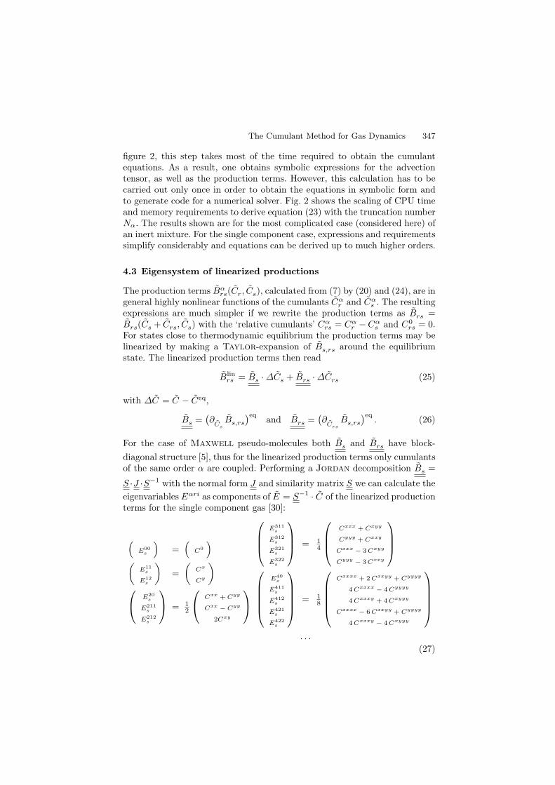
The Cumulant Method for Gas Dynamics 347
figure 2, this step takes most of the time required to obtain the cumulantequations. As a result, one obtains symbolic expressions for the advectiontensor, as well as the production terms. However, this calculation has to becarried out only once in order to obtain the equations in symbolic form andto generate code for a numerical solver. Fig. 2 shows the scaling of CPU timeand memory requirements to derive equation (23) with the truncation numberNα. The results shown are for the most complicated case (considered here) ofan inert mixture. For the single component case, expressions and requirementssimplify considerably and equations can be derived up to much higher orders.
4.3 Eigensystem of linearized productions
The production terms Bαrs(Cr, Cs), calculated from (7) by (20) and (24), are in
general highly nonlinear functions of the cumulants Cαr and Cα
s . The resultingexpressions are much simpler if we rewrite the production terms as Brs =Brs(Cs + Crs, Cs) with the ‘relative cumulants’ Cα
rs = Cαr −Cα
s and C0rs = 0.
For states close to thermodynamic equilibrium the production terms may belinearized by making a Taylor-expansion of Bs,rs around the equilibriumstate. The linearized production terms then read
Blinrs = Bs ·∆Cs + Brs ·∆Crs (25)
with ∆C = C − Ceq,
Bs =(∂
CsBs,rs
)eqand Brs =
(∂
CrsBs,rs
)eq. (26)
For the case of Maxwell pseudo-molecules both Bs and Brs have block-
diagonal structure [5], thus for the linearized production terms only cumulantsof the same order α are coupled. Performing a Jordan decomposition Bs =
S ·J ·S−1 with the normal form J and similarity matrix S we can calculate the
eigenvariables Eαri as components of E = S−1 · C of the linearized productionterms for the single component gas [30]:
(E00
s
)=
(C0
)
(E11
s
E12s
)=
(Cx
Cy
)
E20s
E211s
E212s
= 1
2
Cxx + Cyy
Cxx − Cyy
2Cxy
E311s
E312s
E321s
E322s
= 1
4
Cxxx + Cxyy
Cyyy + Cxxy
Cxxx − 3 Cxyy
Cyyy − 3 Cxxy
E40s
E411s
E412s
E421s
E422s
= 18
Cxxxx + 2 Cxxyy + Cyyyy
4 Cxxxx − 4 Cyyyy
4 Cxxxy + 4 Cxyyy
Cxxxx − 6 Cxxyy + Cyyyy
4 Cxxxy − 4 Cxyyy
. . .
(27)
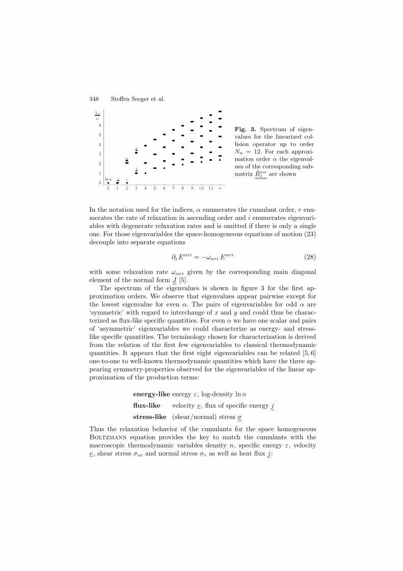
348 Steffen Seeger et al.
0 1 2 3 4 5 6 7 8 9 10 11 120
1
2
3
4
5
6
7
ln n v ε
k
σ
j
α
λαi
ω
Fig. 3. Spectrum of eigen-values for the linearized col-lision operator up to orderNα = 12. For each approxi-mation order α the eigenval-ues of the corresponding sub-matrix Bαα
s are shown
In the notation used for the indices, α enumerates the cumulant order, r enu-merates the rate of relaxation in ascending order and i enumerates eigenvari-ables with degenerate relaxation rates and is omitted if there is only a singleone. For those eigenvariables the space-homogeneous equations of motion (23)decouple into separate equations
∂tEαri = −ωαriE
αri (28)
with some relaxation rate ωαri given by the corresponding main diagonalelement of the normal form J [5].
The spectrum of the eigenvalues is shown in figure 3 for the first ap-proximation orders. We observe that eigenvalues appear pairwise except forthe lowest eigenvalue for even α. The pairs of eigenvariables for odd α are‘symmetric’ with regard to interchange of x and y and could thus be charac-terized as flux-like specific quantities. For even α we have one scalar and pairsof ‘asymmetric’ eigenvariables we could characterize as energy- and stress-like specific quantities. The terminology chosen for characterization is derivedfrom the relation of the first few eigenvariables to classical thermodynamicquantities. It appears that the first eight eigenvariables can be related [5, 6]one-to-one to well-known thermodynamic quantities which have the three ap-pearing symmetry-properties observed for the eigenvariables of the linear ap-proximation of the production terms:
energy-like energy ε, log-density lnn
flux-like velocity v , flux of specific energy j
stress-like (shear/normal) stress σ
Thus the relaxation behavior of the cumulants for the space homogeneousBoltzmann equation provides the key to match the cumulants with themacroscopic thermodynamic variables density n, specific energy ε, velocityv , shear stress σ and normal stress σ as well as heat flux j :
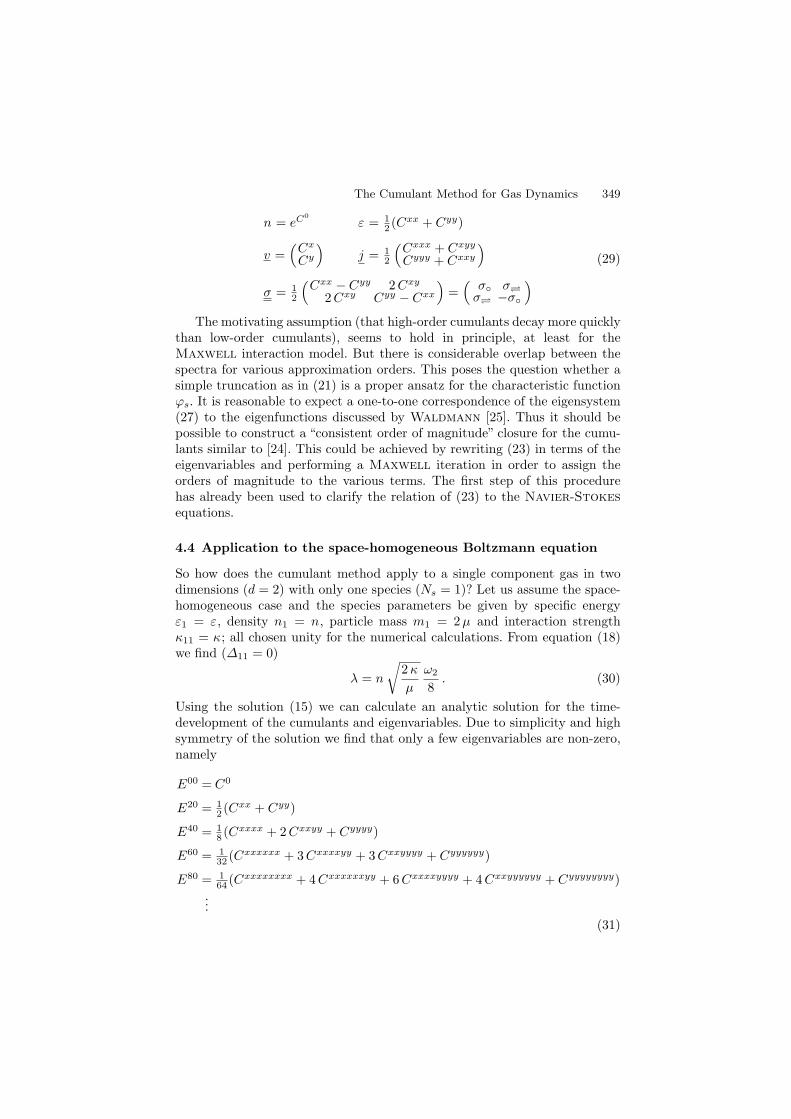
The Cumulant Method for Gas Dynamics 349
n = eC0
ε = 12 (Cxx + Cyy)
v =(Cx
Cy
)j = 1
2
(Cxxx + Cxyy
Cyyy + Cxxy
)
σ = 12
(Cxx − Cyy 2Cxy
2Cxy Cyy − Cxx
)=(σ σ
σ −σ)
(29)
The motivating assumption (that high-order cumulants decay more quicklythan low-order cumulants), seems to hold in principle, at least for theMaxwell interaction model. But there is considerable overlap between thespectra for various approximation orders. This poses the question whether asimple truncation as in (21) is a proper ansatz for the characteristic functionϕs. It is reasonable to expect a one-to-one correspondence of the eigensystem(27) to the eigenfunctions discussed by Waldmann [25]. Thus it should bepossible to construct a “consistent order of magnitude” closure for the cumu-lants similar to [24]. This could be achieved by rewriting (23) in terms of theeigenvariables and performing a Maxwell iteration in order to assign theorders of magnitude to the various terms. The first step of this procedurehas already been used to clarify the relation of (23) to the Navier-Stokes
equations.
4.4 Application to the space-homogeneous Boltzmann equation
So how does the cumulant method apply to a single component gas in twodimensions (d = 2) with only one species (Ns = 1)? Let us assume the space-homogeneous case and the species parameters be given by specific energyε1 = ε, density n1 = n, particle mass m1 = 2µ and interaction strengthκ11 = κ; all chosen unity for the numerical calculations. From equation (18)we find (∆11 = 0)
λ = n
√2κ
µ
ω2
8. (30)
Using the solution (15) we can calculate an analytic solution for the time-development of the cumulants and eigenvariables. Due to simplicity and highsymmetry of the solution we find that only a few eigenvariables are non-zero,namely
E00 = C0
E20 = 12 (Cxx + Cyy)
E40 = 18 (Cxxxx + 2Cxxyy + Cyyyy)
E60 = 132 (Cxxxxxx + 3Cxxxxyy + 3Cxxyyyy + Cyyyyyy)
E80 = 164 (Cxxxxxxxx + 4Cxxxxxxyy + 6Cxxxxyyyy + 4Cxxyyyyyy + Cyyyyyyyy)
...
(31)
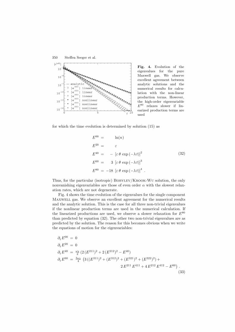
350 Steffen Seeger et al.
0 5 1010
-16
10-13
10-10
10-7
10-4
10-1
analytic
|e(40)
| linear
|e(60)
| linear
|e(80)
| linear
|e(40)
| nonlinear
|e(60)
| nonlinear
|e(80)
| nonlinear
t
|e(α0)|Fig. 4. Evolution of theeigenvalues for the pureMaxwell gas. We observeexcellent agreement betweenanalytic solutions and thenumerical results for calcu-lation with the non-linearproduction terms. However,the high-order eigenvariableE80 relaxes slower if lin-earized production terms areused
for which the time evolution is determined by solution (15) as
E00 = ln(n)
E20 = ε
E40 = − [ε θ exp (−λ t)]2
E60 = 3 [ε θ exp (−λ t)]3
E80 = −18 [ε θ exp (−λ t)]4 .
(32)
Thus, for the particular (isotropic) Bobylev/Krook-Wu solution, the onlynonvanishing eigenvariables are those of even order α with the slowest relax-ation rates, which are not degenerate.
Fig. 4 shows the time evolution of the eigenvalues for the single componentMaxwell gas. We observe an excellent agreement for the numerical resultsand the analytic solution. This is the case for all three non-trivial eigenvaluesif the nonlinear production terms are used in the numerical calculation. Ifthe linearized productions are used, we observe a slower relaxation for E80
than predicted by equation (32). The other two non-trivial eigenvalues are aspredicted by the solution. The reason for this becomes obvious when we writethe equations of motion for the eigenvariables:
∂tE00 = 0
∂tE20 = 0
∂tE40 = ω2
2 (2 (E211)2 + 2 (E212)2 − E40)
∂tE60 = 3ω2
4
(3 ((E311)2 + (E312)2 + (E321)2 + (E322)2)+
2E211E411 + 4E212E412 − E60).
(33)
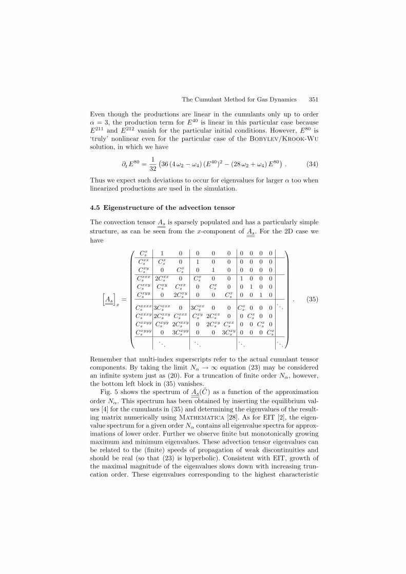
The Cumulant Method for Gas Dynamics 351
Even though the productions are linear in the cumulants only up to orderα = 3, the production term for E40 is linear in this particular case becauseE211 and E212 vanish for the particular initial conditions. However, E80 is‘truly’ nonlinear even for the particular case of the Bobylev/Krook-Wu
solution, in which we have
∂tE80 =
1
32
(36 (4ω2 − ω4) (E40)2 − (28ω2 + ω4)E
80). (34)
Thus we expect such deviations to occur for eigenvalues for larger α too whenlinearized productions are used in the simulation.
4.5 Eigenstructure of the advection tensor
The convection tensor As is sparsely populated and has a particularly simple
structure, as can be seen from the x-component of As. For the 2D case we
have
[As
]x
=
Cxs 1 0 0 0 0 0 0 0 0
Cxxs Cx
s 0 1 0 0 0 0 0 0
Cxys 0 Cx
s 0 1 0 0 0 0 0
Cxxxs 2Cxx
s 0 Cxs 0 0 1 0 0 0
Cxxys Cxy
s Cxxs 0 Cx
s 0 0 1 0 0
Cxyys 0 2Cxy
s 0 0 Cxs 0 0 1 0
Cxxxxs 3Cxxx
s 0 3Cxxs 0 0 Cx
s 0 0 0. . .
Cxxxys 2Cxxy
s Cxxxs Cxy
s 2Cxxs 0 0 Cx
s 0 0
Cxxyys Cxyy
s 2Cxxys 0 2Cxy
s Cxxs 0 0 Cx
s 0
Cxyyys 0 3Cxyy
s 0 0 3Cxys 0 0 0 Cx
s
. . .. . .
. . .. . .
. (35)
Remember that multi-index superscripts refer to the actual cumulant tensorcomponents. By taking the limit Nα → ∞ equation (23) may be consideredan infinite system just as (20). For a truncation of finite order Nα, however,the bottom left block in (35) vanishes.
Fig. 5 shows the spectrum of As(C ) as a function of the approximation
order Nα. This spectrum has been obtained by inserting the equilibrium val-ues [4] for the cumulants in (35) and determining the eigenvalues of the result-ing matrix numerically using Mathematica [28]. As for EIT [2], the eigen-value spectrum for a given orderNα contains all eigenvalue spectra for approx-imations of lower order. Further we observe finite but monotonically growingmaximum and minimum eigenvalues. These advection tensor eigenvalues canbe related to the (finite) speeds of propagation of weak discontinuities andshould be real (so that (23) is hyperbolic). Consistent with EIT, growth ofthe maximal magnitude of the eigenvalues slows down with increasing trun-cation order. These eigenvalues corresponding to the highest characteristic

352 Steffen Seeger et al.
5 10 15 20
- 7.5
- 5
- 2.5
0
2.5
5
7.5
−7.5
1 5 10 15
−5.0
−2.5
0.0
2.5
5.0
Nα
λi−vx√ε
Fig. 5. Eigenspectrum of As(C ) in equilibrium as it depends on the order of ap-
proximation order Nα. For each order, only the newly appearing spectral values areplotted. We observe a finite maximum magnitude, growing monotonically with Nα
speeds evaluated in equilibrium play an important role in modeling shockstructures, as for shock speeds beyond that value unphysical sub-shocks ap-pear in the solutions of the approximate equations [31, 32]. This implies thatmany moments or cumulants have to be considered for fast shocks and mightbe considered a drawback of the cumulant method and moment methods ingeneral.
Solving (29) for the (low-order) cumulants, and inserting these into (35),we can calculate [33] the dependence of the convection tensor eigen-spectrumon the classical variables. For this, one variable has been varied and for theothers equilibrium values have been assumed. We find that demanding hy-perbolicity of the cumulant equations, which requires real eigenvalues for allcomponents of As, imposes different possible constraints on the domain of
allowed eigenvariable values. The first case is that no constraints are imposed,as is the case for vx and vy. An arbitrary mean velocity just produces a shiftof the eigenvalue spectrum of As, as we would expect from a set of equations
with Galileian invariance. The same situation is observed for the shear stressσ, which does not influence the spectrum at all. The second case is observedfor the energy density ε, where the spectra for both the x and y componentimpose a lower bound on ε, independent of Nα. With the third case, bounded-ness of the normal stress σ, jx and jy is imposed but for two different reasons:for σ, the x and y component of As impose either an upper or a lower bound
which are the same for any Nα. For j , however, one As component imposes
The Cumulant Method for Gas Dynamics 353
both upper and lower bounds and the other component of As does not impose
any bounds. But we also observe the paradoxical situation that the intervalof allowed jx-values for (23) to be hyperbolic becomes smaller with increasingNα. Whether the allowed interval remains finite or converges to the empty setfor Nα → ∞ remains an open question. We note that this might not be thecase in real flow situations, where other cumulants may have non-equilibriumvalues, thereby possibly compensating this effect. Thus, ‘not too far’ fromequilibrium, (23) might be characterized as a hyperbolic system of partialdifferential equations.
4.6 Numerical scheme
There are several modern, robust numerical methods for solving a time-dependent hyperbolic system of partial differential equations (see, for in-stance [34–38]). However, most of them rely on a conservation or balance lawformulation of the governing equations. Unfortunately we are not able to finda balance law formulation for the cumulants directly, as the convection tensorcomponents are not Jacobian matrices. The moment equations are equationsin balance form, so this might be a possible set of equations to use with thesemethods. But, this would ultimately require (re-)construction of the fluxesfrom moment values: We would have to calculate the cumulant values frommoments and then the fluxes from the cumulants. Though theoretically possi-ble (from (22) and the inverse relation) this could lead to numerical difficultiesdue to introduction of round-off errors in each iteration step [26].
If we would like to use finite element methods for discretization and nu-merical solution the problem appears that the required variational forms areusually not symmetric and therefore require stabilization [39]. On the otherhand it is well known [40] that for systems where an analytic form of theentropy density is exists, the equations of motion become symmetric in aparticular set of ‘entropic’ variables. Applying finite element discretizationsto these symmetric hyperbolic equations it can be shown that the numeri-cal solution will have the same (thermodynamic) stability properties as thecontinuous equations [41]. Except for necessary conditions, existence and con-struction of entropy functionals operating on the characteristic function hasnot been discussed in the literature so far.
We therefore choose an explicit finite difference approximation of (23), butshould be aware that these methods are known not to be suited for problemswith discontinuous solutions, such as shocks. We start by choosing a regular,orthogonal grid of spacing dt in time and dr in space to discretize the space andtime domain. Let (t, x) denote a grid point and ei the unit vector in direction i.Then we may approximate the derivatives using the following finite differenceratios of first and second order. Thus we approximate the differentials in (23)by
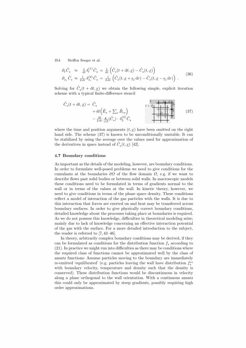
354 Steffen Seeger et al.
∂t Cs ≈ 1dt δ
(1)t Cs = 1
dt
(Cs(t+ dt, x)− Cs(t, x)
)
∂xiCs ≈ 1
2 dr δ(2)xiCs = 1
2 dr
(Cs(t, x+ ei dr)− Cs(t, x− ei dr)
).
(36)
Solving for Cs(t + dt, x) we obtain the following simple, explicit iterationscheme with a typical finite-difference stencil
Cs(t+ dt, x) = Cs
+ dt(Es +
∑r Brs
)
− dt2 dr As(Cs) · δ(2)x Cs
dr
dr
t
y
x
t + dt
(37)
where the time and position arguments (t, x) have been omitted on the righthand side. The scheme (37) is known to be unconditionally unstable. It canbe stabilized by using the average over the values used for approximation ofthe derivatives in space instead of Cs(t, x) [42].
4.7 Boundary conditions
As important as the details of the modeling, however, are boundary conditions.In order to formulate well-posed problems we need to give conditions for thecumulants at the boundaries ∂Ω of the flow domain Ω, e.g. if we want todescribe flows past solid bodies or between solid walls. In macroscopic modelsthese conditions need to be formulated in terms of gradients normal to thewall or in terms of the values at the wall. In kinetic theory, however, weneed to give conditions in terms of the phase space density. These conditionsreflect a model of interaction of the gas particles with the walls. It is due tothis interaction that forces are exerted on and heat may be transferred acrossboundary surfaces. In order to give physically correct boundary conditions,detailed knowledge about the processes taking place at boundaries is required.As we do not possess this knowledge, difficulties in theoretical modeling arise;mainly due to lack of knowledge concerning an effective interaction potentialof the gas with the surface. For a more detailed introduction to the subject,the reader is referred to [7, 43–46].
In theory, arbitrarily complex boundary conditions may be derived, if theycan be formulated as conditions for the distribution function fs according to(21). In practice we might run into difficulties as there may be conditions wherethe required class of functions cannot be approximated well by the class ofansatz functions: Assume particles moving to the boundary are immediatelyre-emitted ‘equilibrated’ (e.g. particles leaving the wall have distribution f eq
s
with boundary velocity, temperature and density such that the density isconserved). These distribution functions would be discontinuous in velocityalong a plane orthogonal to the wall orientation. With a continuous ansatzthis could only be approximated by steep gradients, possibly requiring highorder approximations.
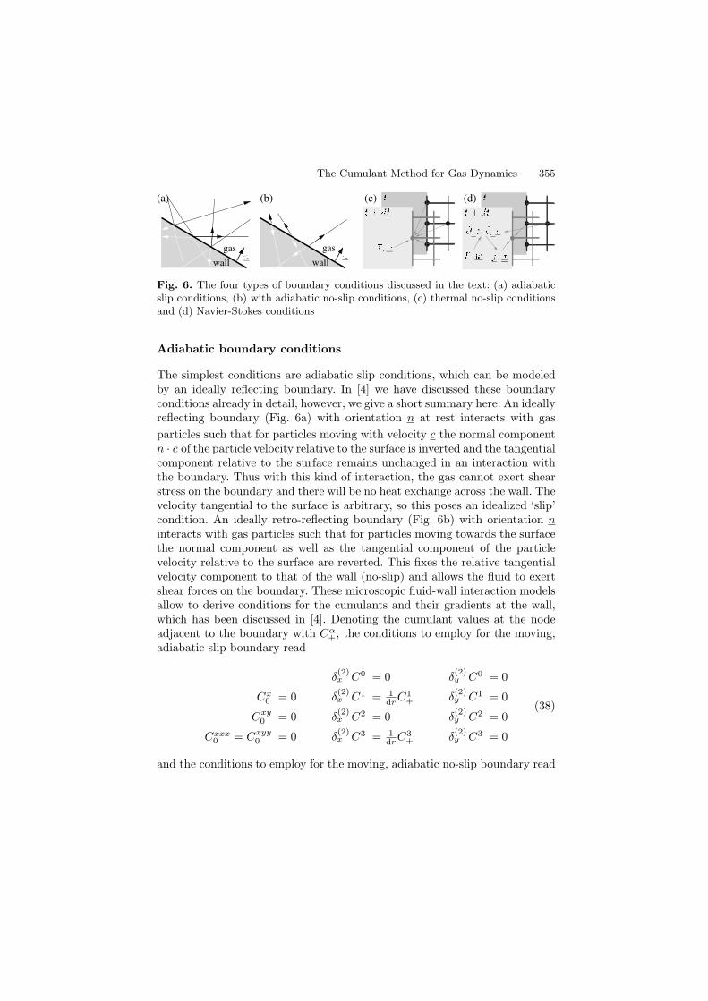
The Cumulant Method for Gas Dynamics 355
gas
wall wall
gas
(c)(b) (d)(a)
Fig. 6. The four types of boundary conditions discussed in the text: (a) adiabaticslip conditions, (b) with adiabatic no-slip conditions, (c) thermal no-slip conditionsand (d) Navier-Stokes conditions
Adiabatic boundary conditions
The simplest conditions are adiabatic slip conditions, which can be modeledby an ideally reflecting boundary. In [4] we have discussed these boundaryconditions already in detail, however, we give a short summary here. An ideallyreflecting boundary (Fig. 6a) with orientation n at rest interacts with gas
particles such that for particles moving with velocity c the normal componentn · c of the particle velocity relative to the surface is inverted and the tangentialcomponent relative to the surface remains unchanged in an interaction withthe boundary. Thus with this kind of interaction, the gas cannot exert shearstress on the boundary and there will be no heat exchange across the wall. Thevelocity tangential to the surface is arbitrary, so this poses an idealized ‘slip’condition. An ideally retro-reflecting boundary (Fig. 6b) with orientation ninteracts with gas particles such that for particles moving towards the surfacethe normal component as well as the tangential component of the particlevelocity relative to the surface are reverted. This fixes the relative tangentialvelocity component to that of the wall (no-slip) and allows the fluid to exertshear forces on the boundary. These microscopic fluid-wall interaction modelsallow to derive conditions for the cumulants and their gradients at the wall,which has been discussed in [4]. Denoting the cumulant values at the nodeadjacent to the boundary with Cα
+, the conditions to employ for the moving,adiabatic slip boundary read
δ(2)x C0 = 0 δ
(2)y C0 = 0
Cx0 = 0 δ
(2)x C1 = 1
drC1+ δ
(2)y C1 = 0
Cxy0 = 0 δ
(2)x C2 = 0 δ
(2)y C2 = 0
Cxxx0 = Cxyy
0 = 0 δ(2)x C3 = 1
drC3+ δ
(2)y C3 = 0
(38)
and the conditions to employ for the moving, adiabatic no-slip boundary read

356 Steffen Seeger et al.
δ(2)x C0 = 0 δ
(2)y C0 = 0
C10 = w δ
(2)x C1 = 1
drC1+ δ
(2)y C1 = 0
δ(2)x C2 = 0 δ
(2)y C2 = 0
C30 = 0 δ
(2)x C3 = 1
drC3+ δ
(2)y C3 = 0
(39)
where w denotes the wall velocity.
Thermal no-slip conditions
An important drawback of the adiabatic boundary conditions is the fact thatheat dissipated in the flow region may not be transported out of the flowregion. This is a considerable deficiency as almost all steady flow regimesrequire some kind of transport of the heat generated by dissipation out ofthe flow region. The main problem is that – for the two kinds of ideallyreflective wall – we cannot prescribe wall velocity and temperature and havethe gas develop stress and heat flux in response to the flow conditions at thewall with the (quite academic) boundary conditions presented above. For thethermal no-slip boundary conditions (Fig. 6c) used in the simulations we treatboundary nodes just as interior fluid nodes. The gradients in n-direction areapproximated by (first-order) one-sided differences. In each update, the wallvelocity and the wall temperature substitute the value of C1 and the traceof C2. Otherwise the node is updated according to (37). This prescribes walltemperature and wall velocity at the boundary node. Shear stress at the walland heat flux across the wall develop due to the gradients in the cumulantsbuilding up.
Navier-stokes conditions
In [5] we have demonstrated calculation of the production terms for theMaxwell gas. By considering states close to equilibrium for a single-componentgas we found that the Jacobian of the production terms with regard to the cu-mulants is block-diagonal. This allows the definition of a set of eigenvariablesof the linearized production terms. It turns out that the first eigenvariables canbe related one by one to well-known macroscopic quantities, namely particledensity n, mean particle velocity v , mean energy ε, stress σ and flux of specificenergy j . Performing the fist step of a Maxwell iteration [47], we recover thewell-known constitutive relations for a Newtonian fluid with heat conductionaccording to Fouriers law. This motivates the Navier-Stokes boundary condi-tions (Fig. 6d): First we calculate the (classical) eigenvariables for the bound-ary node and the fluid node next to the boundary. Then, for the boundarynode, replace v and specific ε by the wall velocity w and specific energy givenby the wall temperature T . Further we approximate the gradients in velocityand energy by one-sided differences and calculate σ and q from their constitu-tive relations. Now the corresponding cumulant values for the boundary node
The Cumulant Method for Gas Dynamics 357
are obtained by the relation between the cumulants and the eigenvariablesas obtained from the Maxwell iteration (given in [5]). With these boundaryconditions employed for the numerical scheme (37) we can simulate variousflow conditions that result in a stationary, non-equilibrium regime. However,in some cases properties of flows in the Navier-Stokes regime are reproduced,in other cases qualitative features of a rather dilute gas, depending on theboundary conditions employed.
5 Summary
We gave a comprehensive overview of the theory behind the cumulant method,the main results about the resulting equations and their properties, as wellas a simple numerical scheme and possible boundary conditions to apply. Themain ansatz is a Taylor expansion of the second characteristic function. Fromthat ansatz, a set of moment equations can be derived by symbolic calcula-tion up to (in principle) arbitrary high orders of approximation. Applying themethod of deriving equations for the cumulants for the special case of a space-homogeneous gas close to a equilibrium state we can linearize the productionterms and determine an eigensystem of the production terms. The low ordereigen-variables can be related one-to-one to classic thermodynamic quantities.Next we have compared a numerical solution of the space-homogeneous equa-tions to the exact Boblev/Krook-Wu solution. We find that the numericalsolution coincides with the exact solution if the fully non-linear productionterms are used. For the linearized production terms, relaxation rates may beunder-estimated. The eigensystem of the advection tensor characterizes thesystem as hyperbolic as long as the system is not too far from equilibrium.The application of modern numerical methods appears to be difficult as thecumulant equations are not in symmetric form. Construction of symmetricequations would be possible if an entropy density could be given as a func-tion of the cumulants. How this can be achieved remains an open question, asso far entropy functionals that operate on the first (or second) characteristicfunction have not been discussed extensively in the literature. Despite that,a simple finite difference scheme and microscopically or phenomenologicallymotivated boundary conditions have been given that can be used to obtainnumerical solutions for simple flow problems.
References
1. H. Grad. On the kinetic theory of rarefied gases. Comm. Pure Appl. Math.,2:331–407, 1949.
2. I. Muller and T. Ruggeri. Rational Extended Thermodynamics, volume 37 ofSpringer Tracts in Natural Philosophy. Springer-Verlag, New York, Berlin, Hei-delberg, 2nd edition, 1998.
358 Steffen Seeger et al.
3. B. C. Eu. Kinetic Theory and Irreversible Thermodynamics, chapter 10.7 Mod-ified Moment Method, pages 365–386. John Wiley & Sons, New York, 1992.
4. S. Seeger and K. H. Hoffmann. The cumulant method for computational kinetictheory. Continuum Mech. Thermodyn., 12:403–421, 2000.
5. S. Seeger and K. H. Hoffmann. The cumulant method applied to a mixture ofMaxwell gases. Continuum Mech. Thermodyn., 14(2):321–335, 2002. see alsoErratum: CMT 16(5):515, 2004.
6. S. Seeger. The Cumulant Method. Phd thesis, Chemnitz University of Tech-nology, Chemnitz, September 2003. http://archiv.tu-chemnitz.de/pub/
2003/0120.7. C. Cercignani, R. Illner, and M. Pulvirenti. The Mathematical Theory of Dilute
Gases, volume 106 of Applied Mathematical Sciences. Springer-Verlag, 1994.8. J. O. Hirschfelder, C. F. Curtiss, and R. B. Bird. Molecular Theory of Gases and
Liquids. Structure of Matter Series. John Wiley & Sons, New York, Chinchester,Brisbane, 2nd edition, 1964.
9. L. Boltzmann. Vorlesungen uber Gastheorie, volume I, chapter Abschnitt III.,pages 153–176. J.A. Barth Verlag, Leipzig, 1896.
10. E. Lukacs. Characteristic Functions. Griffin’s Statistical Monographs andCourses. Charles Griffin & Company, London, 2nd edition, 1970.
11. A. V. Bobylev. The Fourier transform method in the theory of the Boltzmannequation for Maxwell molecules. Doklady Akad. Nauk SSSR, 225:1041–1044,1975. in Russian.
12. A. V. Bobylev. The theory of the nonlinear spatially uniform Boltzmann equa-tion for Maxwell molecules. Sov. Sci. Rev. C: Math. Phys., 7:111–233, 1988.
13. C. Cercignani. The Boltzmann Equation and Its Applications, volume 67 ofApplied Mathematical Sciences. Springer, 1988.
14. A. V. Bobylev. Exact solutions of the Boltzmann equation. Dokl. Akad. NaukSSSR, 225(6):1296–1299, 1975. in Russian.
15. M. Krook and T. Wu. Exact solutions of the Boltzmann equation. Phys. Fluids,20(10):1589–1595, 1977.
16. M. Krook and T.T. Wu. Exact solutions of Boltzmann equations for multicom-ponent systems. Phys. Rev. Lett., 38(18):991–993, 1977.
17. B. Wennberg. On moments and uniqueness for solutions to the space homoge-neous Boltzmann equation. Transp. Theor. Stat. Phys., 23:533–539, 1994.
18. L. Arkeryd, R. Esposito, and M. Pulverenti. The Boltzmann equation for weaklyinhomogeneous data. Comm. Math. Phys., 111:393–407, 1987.
19. W. Loose and S. Hess. Nonequilibrium velocity distribution function of gases:Kinetic theory and molecular dynamics. Phys. Rev. A, 37(6):2099–2111, 1988.
20. S. Hess and M. Malek Mansour. Temperature profile of a dilute gas undergoinga plane Poiseuille flow. Physica A, 272:481–496, 1999.
21. Y. Sone, K. Aoki, S. Takata, H. Sugimoto, and A. V. Bobylev. Inappropriate-ness of the heat-conduction equation for description of a temperature field of astationary gas in the continuum limit: Examination by asymptotic analysis andnumerical computation of the Boltzmann equation. Phys. Fluids, 8(2):628–638,1996.
22. D. Reitebuch and W. Weiss. Application of high moment theory to the planeCouette flow. Continuum Mech. Thermodyn., 4:217–225, 1999.
23. C. D. Levermore. Moment closure hierarchies for kinetic theories. J. Stat. Phys.,83(5/6):1021–1065, 1996.
The Cumulant Method for Gas Dynamics 359
24. I. Muller, D. Reitebuch, and W. Weiss. Extended thermodynamics – consistentin order of magnitude. Continuum Mech. Thermodyn., 15:113–146, 2002.
25. L. Waldmann. Transporterscheinungen in Gasen von mittlerem Druck, volumeXII of Handbuch der Physik, pages 295–514. Springer-Verlag, Berlin, 1958.
26. M. Torrilhon, J. D. Au, and H. Struchtrup. Explicit fluxes and productionsfor large systems of the moment method based on extended thermodynamics.Continuum Mech. Thermodyn., 15(1):97–111, 2002.
27. B. C. Eu. Kinetic Theory and Irreversible Thermodynamics. John Wiley &Sons, Inc., New York, Chichester, Brisbane, 1992.
28. Wolfram Research, Inc. Mathematica, Version 5.0. Champaign, Illinois, 2004.29. S. Seeger and K. H. Hoffmann. On symbolic derivation of the cumulant equa-
tions. Comp. Phys. Comm., 168(3):165–176, 2005.30. S. Seeger. Cumulant method implementation for mathematica.
http://www.tu-chemnitz.de/pub/2003/0120, March 2003.31. W. Weiss. Continuous shock structure in extended thermodynamics. Phys. Rev.
E, 52(6):R5760–R5763, 1995.32. G. Boillat and T. Ruggeri. On the shock structure problem for hyperbolic
system of balance laws and convex entropy. Continuum Mech. Thermodyn.,10(5):285–292, 1998.
33. S. Seeger and K. H. Hoffmann. On the domain of hyperbolicity of the cumulantequations. J. Stat. Phys., 121(1–2):75–90, 2005.
34. E. F. Toro. Riemann solvers and numerical methods for fluid dynamics: a prac-tical introduction. Springer Verlag, Berlin, Heidelberg, New York, 2nd edition,1999.
35. D. Kroner, M. Ohlberger, and C. Rohde, editors. An Introduction to RecentDevelopments in Theory and Numerics for Conservation Laws, volume 5 ofLecture Notes in Computational Science and Engineering, Berlin, Heidelberg,New York, 1999. International School on Theory and Numerics for ConservationLaws 20–24th October, 1997, Springer.
36. T. J. Barth and H. Deconinck, editors. High-Order Methods for ComputationalPhysics, volume 9 of Lecture Notes in Computational Science and Engineering.Springer, Berlin, Heidelberg, New York, 1999.
37. E. Godlewski and P.-A. Raviart. Numerical Approximation of Hyperbolic Sys-tems of Conservation Laws, volume 118 of Applied Mathematical Sciences.Springer, New York, Heidelberg, 1996.
38. M. Fey, editor. Hyperbolic Problems: Theory, Numerics, Applications. Num-ber 129 in International Series of Numercial Mathematics. Birkhauser Verlag,Switzerland, 1999.
39. P. Houston and E. Suli. Stabilized hp-finite element approximation of partial dif-ferential equations with nonnegative characteristic form. Journal of Computing,66(2):99–119, 2001.
40. M. Mock. Systems of conservation laws of mixed type. J. Differential Equations,37:70–88, 1980.
41. T. J. R. Hughes and L. P. Franca. A new finite element formulation for compu-tational fluid dynamics: VII. the Stokes problem with various well-posed bound-ary conditions: symmetric formulations that converge for all velocity/pressurespaces. Comput. Methods Appl. Mech. Engrg., 65:85–96, 1987.
42. Lax. Weak solutions of nonlinear hyperbolic equations and their numericalcompuation. Comm. Pure Appl. Math., VII:159–193, 1954.
360 Steffen Seeger et al.
43. J. C. Maxwell. On stresses in rarefied gases arising from inequalities of temper-ature. Phil. Trans. Royal Soc., 170:231–256, 1879.
44. M. Knudsen. The Kinetic Theory of Gases. Methuen, London, 1950.45. A. V. Bogdanov. Interaction of Gases with Surfaces, volume 25 of Lecture Notes
in Physics. Springer, Berlin, Heidelberg, 1995.46. I. Kuscer. Phenomenological aspects of gas-surface interaction. In E. G. D. Do-
hen and W. Fiszdom, editors, Fundamental Problems in Statistical Mechanics,volume IV, pages 441–467. Ossolineum, Warsaw, 1978.
47. E. Ikenberry and C. Truesdell. On the pressures and the flux of energy in a gasaccording to Maxwell’s kinetic theory, I. J. Rational Mech. Anal., 5(1):1–126,1956.
Index
ab-initio calculation 37abinit 37Anderson 203annealing 227annealing schedule 231auxiliary matrices 208average conductance 212
benchmark 41Bezier spline 218binding energy 233boundary conditions 208, 212
call graph 43compiler 43conductance 215conductivity 203critical 203critical disorder 212critical disorder strength 204critical exponent 211, 212, 219critical point 211
density of states 206, 208density-functional 228dimensionless conductance 210disorder 204disorder-driven MIT 203dynamical exponent 206
electronic structure calculations 37extended states 204
Fermi energy 217
finite-size corrections 211finite-size scaling 210, 211
general scaling form 211
hopping 204
insulator 203irrelevant scaling exponent 211iterative diagonalisation schemes 206
jumpshot 46
Kubo-Greenwood formula 206
LAPACK 218leads 216least square fit 211localisation 203localisation length 204, 210, 219
math library 44mesoscopic 203metallic leads 215MIT 203mobility edge 205, 211, 219molecular dynamics 228
one-parameter scaling 210one-parameter scaling hypothesis 203
performance analysis 37
recursion relations 209recursive Green’s function method 206reduced localisation length 210retarded Green’s functions 206

362 Index
scaling form 206scaling theory 203shifting technique 217, 218speedup 45
thermoelectric kinetic coefficients 206transfer-matrix method 206
transition 203
typical conductance 212
universal critical exponent 205
weak localisation 204
1. Volumes in the following three categories will be published in LNCSE:
i) Research monographsii) Lecture and seminar notesiii) Conference proceedings
Those considering a book which might be suitable for the series are strongly advisedto contact the publisher or the series editors at an early stage.
2. Categories i) and ii). These categories will be emphasized by Lecture Notes inComputational Science and Engineering. Submissions by interdisciplinary teams ofauthors are encouraged. The goal is to report new developments – quickly, inform-ally, and in a way that will make them accessible to non-specialists. In the evaluationof submissions timeliness of the work is an important criterion. Texts should be well-rounded, well-written and reasonably self-contained. In most cases the work willcontain results of others as well as those of the author(s). In each case the author(s)should provide sufficient motivation, examples, and applications. In this respect,Ph.D. theses will usually be deemed unsuitable for the Lecture Notes series. Proposalsfor volumes in these categories should be submitted either to one of the series editorsor to Springer-Verlag, Heidelberg, and will be refereed. A provisional judgment on theacceptability of a project can be based on partial information about the work:a detailed outline describing the contents of each chapter, the estimated length, abibliography, and one or two sample chapters – or a first draft. A final decision whetherto accept will rest on an evaluation of the completed work which should include
– at least 100 pages of text;– a table of contents;– an informative introduction perhaps with some historical remarks which should be– accessible to readers unfamiliar with the topic treated;– a subject index.
3. Category iii). Conference proceedings will be considered for publication providedthat they are both of exceptional interest and devoted to a single topic. One (or more)expert participants will act as the scientific editor(s) of the volume. They select thepapers which are suitable for inclusion and have them individually refereed as for ajournal. Papers not closely related to the central topic are to be excluded. Organizersshould contact Lecture Notes in Computational Science and Engineering at theplanning stage.
In exceptional cases some other multi-author-volumes may be considered in thiscategory.
4. Format. Only works in English are considered. They should be submitted incamera-ready form according to Springer-Verlag’s specifications.Electronic material can be included if appropriate. Please contact the publisher.
Editorial Policy
e+authors?SGWID=5-40017-6-71391-0. http://www.springer.com/east/home/math/math
The macros can also be sent on request.
Technical instructions and/or LaT X macros are available via
Lecture Notes are printed by photo-offset from the master-copy delivered in camera-ready form by the authors. For this purpose Springer-Verlag provides technicalinstructions for the preparation of manuscripts. See also Editorial Policy.
Careful preparation of manuscripts will help keep production time short and ensurea satisfactory appearance of the finished book.
The following terms and conditions hold:
Categories i), ii), and iii):Authors receive 50 free copies of their book. No royalty is paid. Commitment topublish is made by letter of intent rather than by signing a formal contract. Springer-Verlag secures the copyright for each volume.
For conference proceedings, editors receive a total of 50 free copies of their volume fordistribution to the contributing authors.
All categories:Authors are entitled to purchase further copies of their book and other Springermathematics books for their personal use, at a discount of 33,3 % directly fromSpringer-Verlag.
General Remarks
Addresses:
Timothy J. BarthNASA Ames Research CenterNAS DivisionMoffett Field, CA 94035, USAe-mail: [email protected]
Michael Griebel
der Universität BonnWegelerstr. 653115 Bonn, Germanye-mail: [email protected]
David E. KeyesDepartment of Applied Physicsand Applied MathematicsColumbia University200 S. W. Mudd Building500 W. 120th StreetNew York, NY 10027, USAe-mail: [email protected]
Risto M. NieminenLaboratory of PhysicsHelsinki University of Technology02150 Espoo, Finlande-mail: [email protected]
Dirk RooseDepartment of Computer ScienceKatholieke Universiteit LeuvenCelestijnenlaan 200A3001 Leuven-Heverlee, Belgiume-mail: [email protected]
Tamar SchlickDepartment of ChemistryCourant Institute of MathematicalSciencesNew York Universityand Howard Hughes Medical Institute251 Mercer StreetNew York, NY 10012, USAe-mail: [email protected]
Tiergartenstrasse 17D-69121 Heidelberg, GermanyTel.: *49 (6221) 487-8185Fax: *49 (6221) 487-8355
Institut für Numerische Simulation
Mathematics Editor at Springer: Martin PetersSpringer-Verlag, Mathematics Editorial IV
e-mail: [email protected]
Lecture Notesin Computational Scienceand Engineering
Vol. 1 D. Funaro, Spectral Elements for Transport-Dominated Equations. 1997. X, 211 pp. Softcover.ISBN 3-540-62649-2
Vol. 2 H. P. Langtangen, Computational Partial Differential Equations. Numerical Methods and Diff-pack Programming. 1999. XXIII, 682 pp. Hardcover. ISBN 3-540-65274-4
Vol. 3 W. Hackbusch, G. Wittum (eds.), Multigrid Methods V. Proceedings of the Fifth European Multi-grid Conference held in Stuttgart, Germany, October 1-4, 1996. 1998. VIII, 334 pp. Softcover.ISBN 3-540-63133-X
Vol. 4 P. Deuflhard, J. Hermans, B. Leimkuhler, A. E. Mark, S. Reich, R. D. Skeel (eds.), Computational
Molecular Dynamics: Challenges, Methods, Ideas. Proceedings of the 2nd International Symposiumon Algorithms for Macromolecular Modelling, Berlin, May 21-24, 1997. 1998. XI, 489 pp. Softcover.ISBN 3-540-63242-5
Vol. 5 D. Kröner, M. Ohlberger, C. Rohde (eds.), An Introduction to Recent Developments in Theory
and Numerics for Conservation Laws. Proceedings of the International School on Theory and Numer-ics for Conservation Laws, Freiburg / Littenweiler, October 20-24, 1997. 1998. VII, 285 pp. Softcover.ISBN 3-540-65081-4
Vol. 6 S. Turek, Efficient Solvers for Incompressible Flow Problems. An Algorithmic and ComputationalApproach. 1999. XVII, 352 pp, with CD-ROM. Hardcover. ISBN 3-540-65433-X
Vol. 7 R. von Schwerin, Multi Body System SIMulation. Numerical Methods, Algorithms, and Software.1999. XX, 338 pp. Softcover. ISBN 3-540-65662-6
Vol. 8 H.-J. Bungartz, F. Durst, C. Zenger (eds.), High Performance Scientific and Engineering Comput-
ing. Proceedings of the International FORTWIHR Conference on HPSEC, Munich, March 16-18, 1998.1999. X, 471 pp. Softcover. ISBN 3-540-65730-4
Vol. 9 T. J. Barth, H. Deconinck (eds.), High-Order Methods for Computational Physics. 1999. VII, 582
pp. Hardcover. ISBN 3-540-65893-9
Vol. 10 H. P. Langtangen, A. M. Bruaset, E. Quak (eds.), Advances in Software Tools for Scientific Com-
puting. 2000. X, 357 pp. Softcover. ISBN 3-540-66557-9
Vol. 11 B. Cockburn, G. E. Karniadakis, C.-W. Shu (eds.), Discontinuous Galerkin Methods. Theory,Computation and Applications. 2000. XI, 470 pp. Hardcover. ISBN 3-540-66787-3
Vol. 12 U. van Rienen, Numerical Methods in Computational Electrodynamics. Linear Systems in Prac-tical Applications. 2000. XIII, 375 pp. Softcover. ISBN 3-540-67629-5
Vol. 13 B. Engquist, L. Johnsson, M. Hammill, F. Short (eds.), Simulation and Visualization on the Grid.
Parallelldatorcentrum Seventh Annual Conference, Stockholm, December 1999, Proceedings. 2000. XIII,301 pp. Softcover. ISBN 3-540-67264-8
Vol. 14 E. Dick, K. Riemslagh, J. Vierendeels (eds.), Multigrid Methods VI. Proceedings of the Sixth Eu-ropean Multigrid Conference Held in Gent, Belgium, September 27-30, 1999. 2000. IX, 293 pp. Softcover.ISBN 3-540-67157-9
Vol. 15 A. Frommer, T. Lippert, B. Medeke, K. Schilling (eds.), Numerical Challenges in Lattice Quan-
tum Chromodynamics. Joint Interdisciplinary Workshop of John von Neumann Institute for Computing,Jülich and Institute of Applied Computer Science, Wuppertal University, August 1999. 2000. VIII, 184
pp. Softcover. ISBN 3-540-67732-1
Vol. 16 J. Lang, Adaptive Multilevel Solution of Nonlinear Parabolic PDE Systems. Theory, Algorithm,and Applications. 2001. XII, 157 pp. Softcover. ISBN 3-540-67900-6
Vol. 17 B. I. Wohlmuth, Discretization Methods and Iterative Solvers Based on Domain Decomposition.
2001. X, 197 pp. Softcover. ISBN 3-540-41083-X
Vol. 18 U. van Rienen, M. Günther, D. Hecht (eds.), Scientific Computing in Electrical Engineering. Pro-ceedings of the 3rd International Workshop, August 20-23, 2000, Warnemünde, Germany. 2001. XII, 428
pp. Softcover. ISBN 3-540-42173-4
Vol. 19 I. Babuška, P. G. Ciarlet, T. Miyoshi (eds.), Mathematical Modeling and Numerical Simulation
in Continuum Mechanics. Proceedings of the International Symposium on Mathematical Modeling andNumerical Simulation in Continuum Mechanics, September 29 - October 3, 2000, Yamaguchi, Japan.2002. VIII, 301 pp. Softcover. ISBN 3-540-42399-0
Vol. 20 T. J. Barth, T. Chan, R. Haimes (eds.), Multiscale and Multiresolution Methods. Theory and Ap-plications. 2002. X, 389 pp. Softcover. ISBN 3-540-42420-2
Vol. 21 M. Breuer, F. Durst, C. Zenger (eds.), High Performance Scientific and Engineering Computing.
Proceedings of the 3rd International FORTWIHR Conference on HPSEC, Erlangen, March 12-14, 2001.2002. XIII, 408 pp. Softcover. ISBN 3-540-42946-8
Vol. 22 K. Urban, Wavelets in Numerical Simulation. Problem Adapted Construction and Applications.2002. XV, 181 pp. Softcover. ISBN 3-540-43055-5
Vol. 23 L. F. Pavarino, A. Toselli (eds.), Recent Developments in Domain Decomposition Methods. 2002.XII, 243 pp. Softcover. ISBN 3-540-43413-5
Vol. 24 T. Schlick, H. H. Gan (eds.), Computational Methods for Macromolecules: Challenges and Ap-
plications. Proceedings of the 3rd International Workshop on Algorithms for Macromolecular Modeling,New York, October 12-14, 2000. 2002. IX, 504 pp. Softcover. ISBN 3-540-43756-8
Vol. 25 T. J. Barth, H. Deconinck (eds.), Error Estimation and Adaptive Discretization Methods in Com-
putational Fluid Dynamics. 2003. VII, 344 pp. Hardcover. ISBN 3-540-43758-4
Vol. 26 M. Griebel, M. A. Schweitzer (eds.), Meshfree Methods for Partial Differential Equations. 2003.IX, 466 pp. Softcover. ISBN 3-540-43891-2
Vol. 27 S. Müller, Adaptive Multiscale Schemes for Conservation Laws. 2003. XIV, 181 pp. Softcover.ISBN 3-540-44325-8
Vol. 28 C. Carstensen, S. Funken, W. Hackbusch, R. H. W. Hoppe, P. Monk (eds.), Computational Elec-
tromagnetics. Proceedings of the GAMM Workshop on "Computational Electromagnetics", Kiel, Ger-many, January 26-28, 2001. 2003. X, 209 pp. Softcover. ISBN 3-540-44392-4
Vol. 29 M. A. Schweitzer, A Parallel Multilevel Partition of Unity Method for Elliptic Partial Differen-
tial Equations. 2003. V, 194 pp. Softcover. ISBN 3-540-00351-7
Vol. 30 T. Biegler, O. Ghattas, M. Heinkenschloss, B. van Bloemen Waanders (eds.), Large-Scale PDE-
Constrained Optimization. 2003. VI, 349 pp. Softcover. ISBN 3-540-05045-0
Vol. 31 M. Ainsworth, P. Davies, D. Duncan, P. Martin, B. Rynne (eds.), Topics in Computational Wave
Propagation. Direct and Inverse Problems. 2003. VIII, 399 pp. Softcover. ISBN 3-540-00744-X
Vol. 32 H. Emmerich, B. Nestler, M. Schreckenberg (eds.), Interface and Transport Dynamics. Compu-tational Modelling. 2003. XV, 432 pp. Hardcover. ISBN 3-540-40367-1
Vol. 33 H. P. Langtangen, A. Tveito (eds.), Advanced Topics in Computational Partial Differential Equa-
tions. Numerical Methods and Diffpack Programming. 2003. XIX, 658 pp. Softcover. ISBN 3-540-01438-1
Vol. 34 V. John, Large Eddy Simulation of Turbulent Incompressible Flows. Analytical and NumericalResults for a Class of LES Models. 2004. XII, 261 pp. Softcover. ISBN 3-540-40643-3
Vol. 35 E. Bänsch (ed.), Challenges in Scientific Computing - CISC 2002. Proceedings of the Confer-ence Challenges in Scientific Computing, Berlin, October 2-5, 2002. 2003. VIII, 287 pp. Hardcover.ISBN 3-540-40887-8
Vol. 36 B. N. Khoromskij, G. Wittum, Numerical Solution of Elliptic Differential Equations by Reduc-
tion to the Interface. 2004. XI, 293 pp. Softcover. ISBN 3-540-20406-7
Vol. 37 A. Iske, Multiresolution Methods in Scattered Data Modelling. 2004. XII, 182 pp. Softcover.ISBN 3-540-20479-2
Vol. 38 S.-I. Niculescu, K. Gu (eds.), Advances in Time-Delay Systems. 2004. XIV, 446 pp. Softcover.ISBN 3-540-20890-9
Vol. 39 S. Attinger, P. Koumoutsakos (eds.), Multiscale Modelling and Simulation. 2004. VIII, 277 pp.Softcover. ISBN 3-540-21180-2
Vol. 40 R. Kornhuber, R. Hoppe, J. Périaux, O. Pironneau, O. Wildlund, J. Xu (eds.), Domain Decompo-
sition Methods in Science and Engineering. 2005. XVIII, 690 pp. Softcover. ISBN 3-540-22523-4
Vol. 41 T. Plewa, T. Linde, V.G. Weirs (eds.), Adaptive Mesh Refinement – Theory and Applications.
2005. XIV, 552 pp. Softcover. ISBN 3-540-21147-0
Vol. 42 A. Schmidt, K.G. Siebert, Design of Adaptive Finite Element Software. The Finite Element Tool-box ALBERTA. 2005. XII, 322 pp. Hardcover. ISBN 3-540-22842-X
Vol. 43 M. Griebel, M.A. Schweitzer (eds.), Meshfree Methods for Partial Differential Equations II.
2005. XIII, 303 pp. Softcover. ISBN 3-540-23026-2
Vol. 44 B. Engquist, P. Lötstedt, O. Runborg (eds.), Multiscale Methods in Science and Engineering.
2005. XII, 291 pp. Softcover. ISBN 3-540-25335-1
Vol. 45 P. Benner, V. Mehrmann, D.C. Sorensen (eds.), Dimension Reduction of Large-Scale Systems.
2005. XII, 402 pp. Softcover. ISBN 3-540-24545-6
Vol. 46 D. Kressner (ed.), Numerical Methods for General and Structured Eigenvalue Problems. 2005.XIV, 258 pp. Softcover. ISBN 3-540-24546-4
Vol. 47 A. Boriçi, A. Frommer, B. Joó, A. Kennedy, B. Pendleton (eds.), QCD and Numerical Analysis
III. 2005. XIII, 201 pp. Softcover. ISBN 3-540-21257-4
Vol. 48 F. Graziani (ed.), Computational Methods in Transport. 2006. VIII, 524 pp. Softcover.ISBN 3-540-28122-3
Vol. 49 B. Leimkuhler, C. Chipot, R. Elber, A. Laaksonen, A. Mark, T. Schlick, C. Schütte, R. Skeel(eds.), New Algorithms for Macromolecular Simulation. 2006. XVI, 376 pp. Softcover. ISBN 3-540-25542-7
Vol. 50 M. Bücker, G. Corliss, P. Hovland, U. Naumann, B. Norris (eds.), Automatic Differentiation:
Applications, Theory, and Implementations. 2006. XVIII, 362 pp. Softcover. ISBN 3-540-28403-6
Vol. 51 A.M. Bruaset, A. Tveito (eds.), Numerical Solution of Partial Differential Equations on Parallel
Computers 2006. XII, 482 pp. Softcover. ISBN 3-540-29076-1
Vol. 52 K.H. Hoffmann, A. Meyer (eds.), Parallel Algorithms and Cluster Computing. 2006. X, 374 pp.Softcover. ISBN 3-540-33539-0
For further information on these books please have a look at our mathematics catalogue at the following
URL: www.springer.com/series/3527
Monographs in Computational Scienceand EngineeringVol. 1 J. Sundnes, G.T. Lines, X. Cai, B.F. Nielsen, K.-A. Mardal, A. Tveito, Computing the Electrical
Activity in the Heart. 2006. XI, 318 pp. Hardcover. ISBN 3-540-33432-7
For further information on this book, please have a look at our mathematics catalogue at the following
URL: www.springer.com/series/7417
Texts in Computational Scienceand EngineeringVol. 1 H. P. Langtangen, Computational Partial Differential Equations. Numerical Methods and Diff-pack Programming. 2nd Edition 2003. XXVI, 855 pp. Hardcover. ISBN 3-540-43416-X

Vol. 2 A. Quarteroni, F. Saleri, Scientific Computing with MATLAB and Octave. 2nd Edition 2006. XIV,318 pp. Hardcover. ISBN 3-540-32612-X
Vol. 3 H. P. Langtangen, Python Scripting for Computational Science. 2nd Edition 2006. XXIV, 736 pp.Hardcover. ISBN 3-540-29415-5
For further information on these books please have a look at our mathematics catalogue at the following
URL: www.springer.com/series/5151