Parallel AlgorithmsPeter Harrison and William Knottenbelt

Email: pgh,wjk@doc.ic.ac.uk

Department of Computing, Imperial College London

ParAlgs–2012 – p.1/65

Course Structure18 lectures6 regular tutorials2 lab-tutorials1 revision lecture-tutorial (optional)

ParAlgs–2012 – p.2/65

Course AssessmentExam (answer 3 out of 4 questions)one assessed courseworkone laboratory exercise

ParAlgs–2012 – p.3/65

Recommended BooksKumar, Grama, Gupta, Karypis. Introductionto Parallel Computing. Benjamin/Cummings.Second Edition, 2002.First Edition, 1994, is OK.Main course textFreeman and Phillips. Parallel NumericalAlgorithms. Prentice-Hall, 1992.Main text for stuff on differential equations

ParAlgs–2012 – p.4/65

Other BooksCosnard, Trystram. Parallel Algorithms andArchitectures. International ThomsonComputer Press, 1995.Foster. Designing and Building ParallelPrograms. Addison-Wesley, 1994.Akl. The Design and Analysis of ParallelAlgorithms. Prentice-Hall, 1989.An old classic

ParAlgs–2012 – p.5/65

Course Outline

Topic No. of lecturesArchitectures & communication networks 4Parallel performance metrics 2Dense matrix algorithms 4Message Passing Interface (MPI) 2Sparse matrix algorithms 2Dynamic search algorithms 4TOTAL 18

ParAlgs–2012 – p.6/65

Computer Architectures

1. SequentialJohn von Neumann model: CPU + MemorySingle Instruction stream, Single Datastream (SISD)Predictable performance of (sequential)algorithms with respect to von Neumannmachine

ParAlgs–2012 – p.7/65

Computer Architectures2. Parallel

Multiple cooperating processors, classifiedby control mechanism, memoryorganisation, interconnection network (IN)Performance of parallel algorithm dependson target architecture and how it is mapped

ParAlgs–2012 – p.8/65

Control MechanismsSingle Instruction stream, Multiple Datastream (SIMD): all processors execute thesame instructions synchronously⇒ good fordata parallelismMultiple Instruction stream, Multiple Datastream (MIMD): processors execute their ownprograms asynchronously⇒ more generalprocess networks (static)divide-and-conquer algorithms (dynamic)

ParAlgs–2012 – p.9/65

Control Mechanisms – hybrid

Single Program, Multiple Data stream(SPMD): all processors run the same programasynchronouslyHybrid SIMD / MIMDalso suitable for data-parallelism but needsexplicit synchronisation

ParAlgs–2012 – p.10/65

Memory Organization1. Message-passing architecture

Several processors with their own (local)memory interact only by message passingover the INDistributed memory architectureMIMD message-passing architecture ≡multicomputer

2. Shared address space architectureSingle address space shared by allprocessors

ParAlgs–2012 – p.11/65

Memory Organization (2)

2. Shared address space architecture (cont.)Multiprocessor architectureUniform memory access (UMA)⇒(average) access time same for all memoryblocks: e.g. single memory bank (orhierarchy)Otherwise non-uniform memory access(NUMA): e.g. global address space isdistributed across the processors’ localmemories (distributed shared memorymultiprocessor)Also cache hierarchies imply less uniformity

ParAlgs–2012 – p.12/65

Interconnection Network1. Static (or direct) networks

Point to point communication amongstprocessorsTypical in message-passing architecturesExamples are ring, mesh, hypercubeTopology critically affects parallel algorithmperformance (see coming lectures)

ParAlgs–2012 – p.13/65

Interconnection Network (2)

2. Dynamic (or indirect) networksConnections between processors areconstructed dynamically during executionusing switches, e.g. crossbars or networksof these such as multistage banyan (ordelta, or omega, or butterfly) networks.Typically used to implement sharedaddress space architecturesBut also in some message-passingalgorithms; e.g. the FFT on a butterfly (seetextbooks)

ParAlgs–2012 – p.14/65

Parallel Random Access MachineThe PRAM is an idealised model ofcomputation on a shared-memory MIMDcomputerFixed number p of processorsUnbounded UMA global memoryAll instructions last one cycleSynchronous operation (‘common clock’) butdifferent instructions are allowed in differentprocessors on the same cycle

ParAlgs–2012 – p.15/65

PRAM memory access modes

Four modes of ‘simultaneous’ memory access (2types of access, 2 modes)

EREW: Exclusive read, exclusive write. WeakestPRAM model, minimum concurrency.

CREW: Concurrent read, exclusive write. Better.CRCW: Concurrent read, concurrent write. Maximum

concurrency. Can simulate on a EREWPRAM (exercise)

ERCW: Exclusive read, concurrent write. Unusual?

ParAlgs–2012 – p.16/65

Concurrent Write SemanticsArbitration is needed to define a uniquesemantics of concurrent write in CRCW andERCW PRAMs

Common All values to be written are the sameArbitrary Pick one writer at randomPriority All processors have a preassigned priorityReduce Write the (generalised) sum of all values

attempting to be written. ‘Sum’ can be anyassociative and commutative operator – cf.‘reduce’ or ‘fold’ of functional languages.

ParAlgs–2012 – p.17/65

PRAM roleNatural extension of the von Neumann modelwith zero cost communication (via sharedmemory)We will use the PRAM to assess thecomplexity of some parallel algorithmsGives an upper bound on performance, e.g.minimum achievable latency

ParAlgs–2012 – p.18/65

Static Interconnection Networks1. Completely connected

direct link between every pair of processorsideal performance but complex andexpensive

2. Starall communication through a special‘central’ processorcentral processor liable to become abottlenecklogically equivalent to a bus – associatedwith shared memory machines (dynamicnetwork)

ParAlgs–2012 – p.19/65

Static Interconnection Networks (2)3. Linear array and ring

connect processors in tandemwith wrap-around gives a ringcommunication via multiple ‘hops’ overlinks through intermediate processorsbasis for quantitative analysis of manyother common networks

ParAlgs–2012 – p.20/65

Static Interconnection Networks (3)4. Mesh

generalisation of linear array (or ring withwrap-around) to more than one dimensionprocessors labelled by rectilinearcoordinateslinks between adjacent processors on eachcoordinate axis (i.e. in each dimension)multiple paths between source anddestination processors

ParAlgs–2012 – p.21/65

Static Interconnection Networks (4)5. Tree

unique path between any pair ofprocessorsprocessors reside at the leaves of the treeInternal nodes may be processors (typicalin static network) or switches (typical indynamic networks)bottlenecks higher up the treecan alleviate by increasing bandwidth athigher levels→ fat tree (e.g. in CM5)

ParAlgs–2012 – p.22/65

Cube NetworksIn a k-ary d-cube topology – of dimension d andradix k – each processor is connected to d others(with wrap-around) and there are k processorsalong each dimension

Regular d-dimensional mesh with kd

processorsProcessors labelled by d digit number withradix k

Ring of p processors is a p-ary 1-cubeWrap-around mesh of p processors is a√

p-ary 2-cubeParAlgs–2012 – p.23/65

Hypercubes

A k-ary d-cube can be formed from k k-ary(d − 1)-cubes by connecting correspondingnodes into ringse.g. composition of rings to form awrap-around meshHypercube ≡ binary d-cubenodes labelled by binary numbers of ddigitseach node connected directly to d othersadjacent nodes differ in exactly one bit

ParAlgs–2012 – p.24/65

Embeddings into HypercubesHypercube is the most richly connected topologywe have considered (apart from completelyconnected) so can we consider other topologiesas embedded subnetworks?1. Ring of 2d nodes

Need to find a sequence of adjacentnodes, with wraparound, in a d-hypercubeAdjacent node labels differ in exactly onebit position

ParAlgs–2012 – p.25/65

Mapping: ring→ hypercube

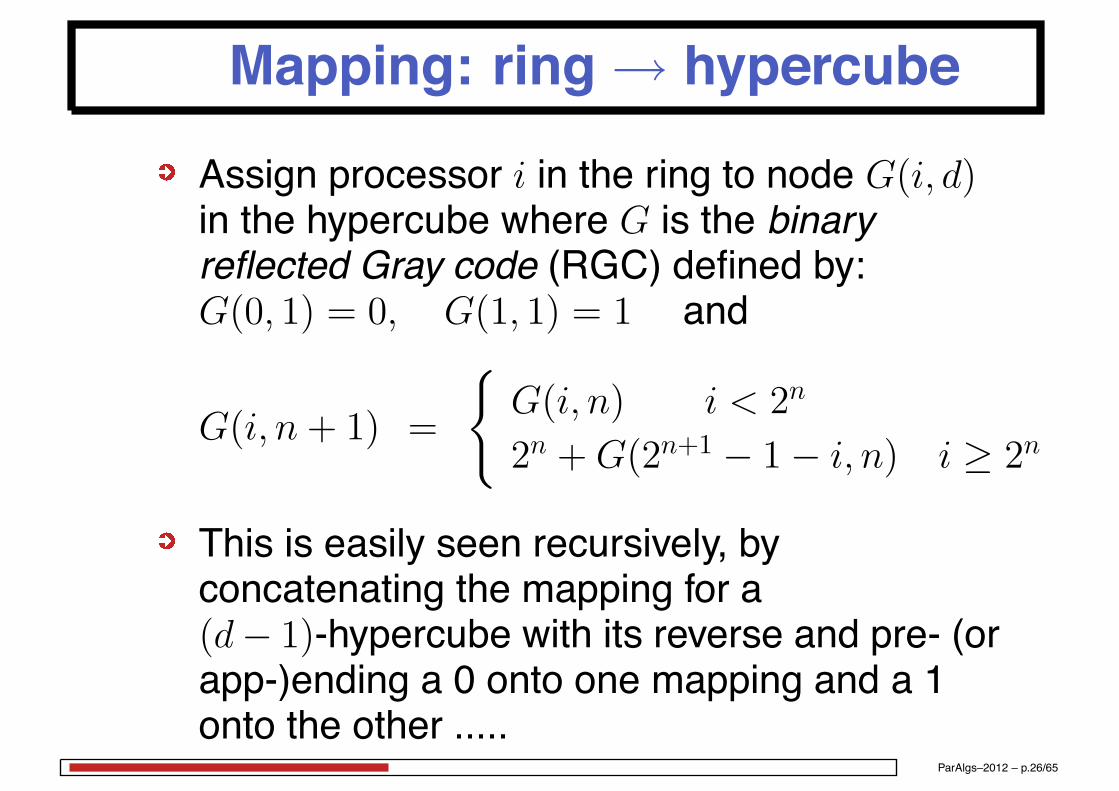
Assign processor i in the ring to node G(i, d)in the hypercube where G is the binaryreflected Gray code (RGC) defined by:G(0, 1) = 0, G(1, 1) = 1 and

G(i, n + 1) =

G(i, n) i < 2n

2n + G(2n+1 − 1 − i, n) i ≥ 2n

This is easily seen recursively, byconcatenating the mapping for a(d− 1)-hypercube with its reverse and pre- (orapp-)ending a 0 onto one mapping and a 1onto the other .....

ParAlgs–2012 – p.26/65

Why is this true?

Proof by induction: a sketch (all that is necessaryhere) is:1. Certainly true for d = 1, when 0 '→ 0 and

1 '→ 1

2. For d ≥ 0, assume successive nodeaddresses in any d-cube ring mapping differin only one bit

3. Hence same applies in each half of the RGCfor a (d + 1)-cube

4. But because of the reflection, the same holdsfor adjacent nodes in different halves.

ParAlgs–2012 – p.27/65

Mapping: mesh→ hypercube

The mapping for an m dimensional mesh isobtained by concatenating the RGCs for eachindividual dimensionThus node (i1, . . . , im) in a 2r1 × . . . × 2rm

mesh maps to node

G(i1, r1) <> . . . <> G(im, rm)

E.g. in an 8 × 8 square mesh, the node atcoordinate (2, 7) maps to hypercube node(0, 1, 1, 1, 0, 0).

ParAlgs–2012 – p.28/65

Mapping: tree→ hypercube

Consider a (complete) binary tree of depth dwith processors at the leaves onlyThis embeds into a d-hypercube as follows,via a many-to-one mapping that maps everynode1. map the root (level 0) to any node, e.g.

(0, . . . , 0)

2. For each node at level j, if mapped tohypercube node !k, map the left child to !k

and the right child to !k with bit j inverted.3. repeat for j = 1, . . . , d

ParAlgs–2012 – p.29/65

Monotonicity of the mapping

Distance between two tree-nodes is 2n forsome n ≥ 1 (difference between d and thelevel of the lowest common ancestor)The corresponding distance in the hypercubeis n – think of bit-changesNodes further apart in the hypercube must befurther apart in the tree, but the converse maynot hold:because of richer hypercube connectivitysome bits might flip backdistant tree-nodes might happen to becloser in the hypercube: d are adjacent

ParAlgs–2012 – p.30/65

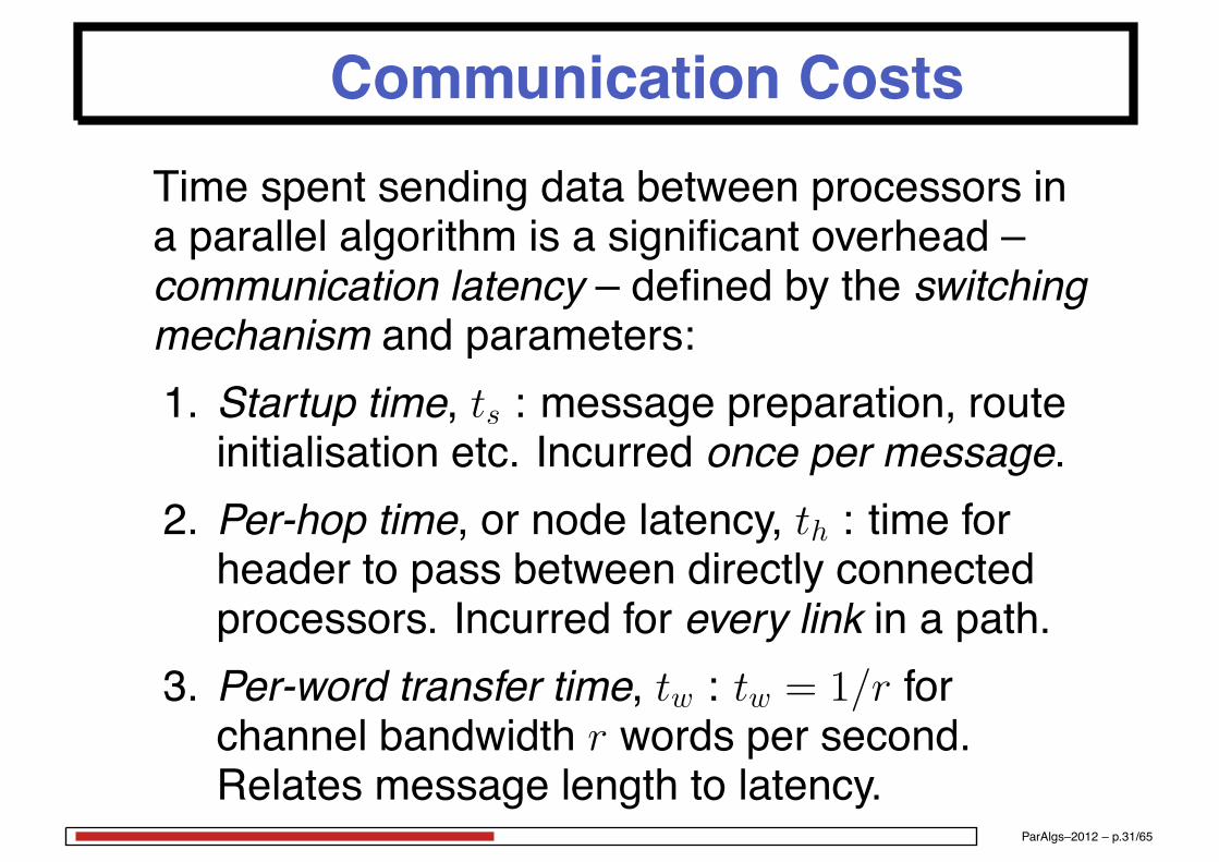
Communication CostsTime spent sending data between processors ina parallel algorithm is a significant overhead –communication latency – defined by the switchingmechanism and parameters:1. Startup time, ts : message preparation, routeinitialisation etc. Incurred once per message.

2. Per-hop time, or node latency, th : time forheader to pass between directly connectedprocessors. Incurred for every link in a path.

3. Per-word transfer time, tw : tw = 1/r forchannel bandwidth r words per second.Relates message length to latency.

ParAlgs–2012 – p.31/65

Switching Mechanisms

1. Store-and-forward routingEach intermediate processor on acommunication path receives an entiremessage and only then sends it on to the nextnode on the pathFor a message of size m words, thecommunication latency on a path of l links is:

tcomm = ts + (mtw + th)l

Typically th is small and so we oftenapproximate tcomm = ts + mtwl

ParAlgs–2012 – p.32/65

Switching Mechanisms (2)

2. Cut-through routingReduce idle time of resources by ‘pipelining’messages along a path ‘in pieces’Messages are advanced to the out-link of anode as they arrive at the in-linkWormhole routing splits messages into flits(flow-control digits) which are then pipelined

ParAlgs–2012 – p.33/65

Wormhole Routing

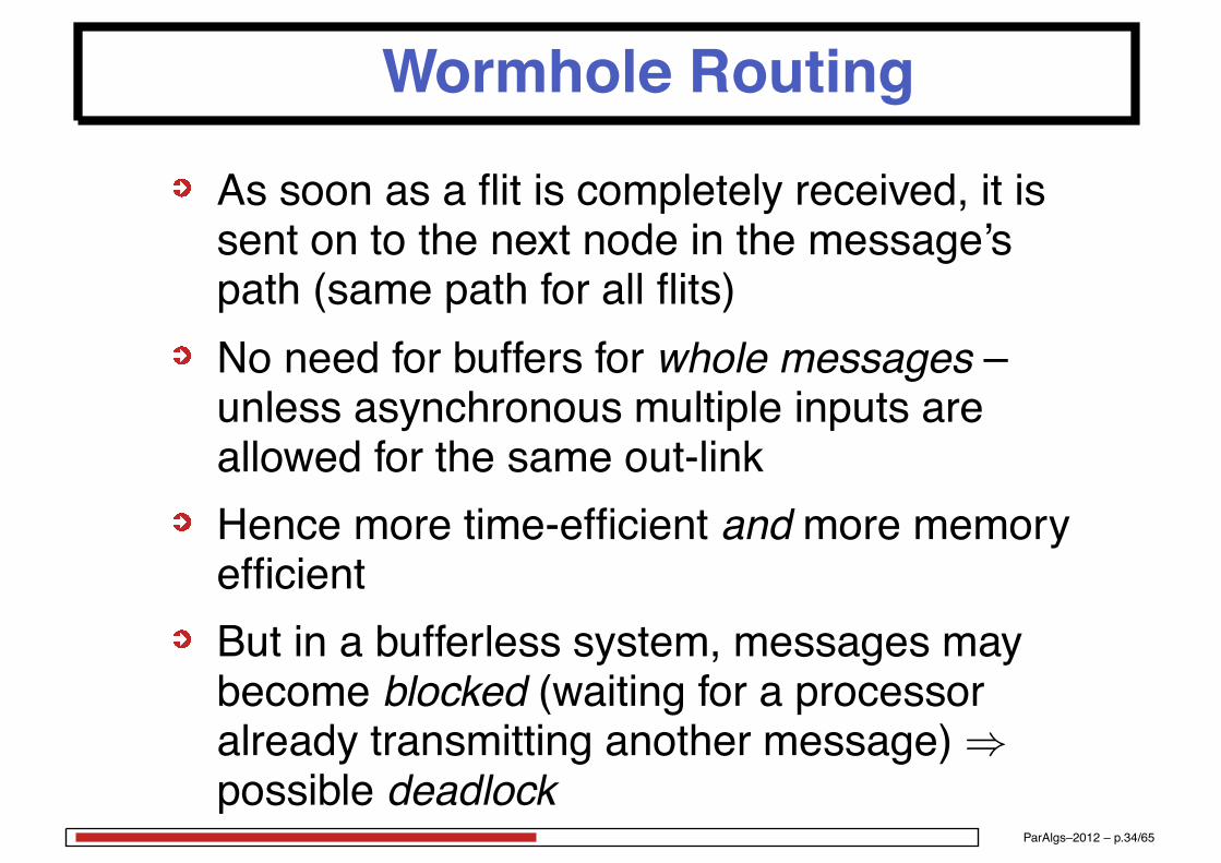
As soon as a flit is completely received, it issent on to the next node in the message’spath (same path for all flits)No need for buffers for whole messages –unless asynchronous multiple inputs areallowed for the same out-linkHence more time-efficient and more memoryefficientBut in a bufferless system, messages maybecome blocked (waiting for a processoralready transmitting another message)⇒possible deadlock

ParAlgs–2012 – p.34/65

Wormhole Routing (2)

On an l-link path, header flit latency = lth

An m-word message will all arrive mtw afterthe headerFor a message of size m words, thecommunication latency on a path of l links istherefore:

tcomm = ts + mtw + lth

Θ(m + l) for cut-through vs. Θ(ml) forstore-and-forwardsimilar for small l (identical for l = 1)

ParAlgs–2012 – p.35/65

Communication Operations

Certain types of computation occur in manyparallel algorithmsSome are implemented naturally by particularcommunication patternsWe consider the following patterns ofcommunication – where the dual operations,with the direction of the communicationreversed, are shown in brackets . . .

ParAlgs–2012 – p.36/65

Communication Patternssimple message transfer between twoprocessors (same for dual)one-to-all broadcast (single nodeaccumulation)all-to-all broadcast (multi-node accumulation)one-to-all personalised (single node gather)all-to-all personalised, or ‘scatter’ (multi-nodegather)more exotic patterns, e.g. permutations

ParAlgs–2012 – p.37/65

Simple Message Transfer

Most basic type of communicationDual operation is of the same typeLatency for single message is :

Tsmt-sf = ts + twml + thl for store-and-forwardroutingTsmt-ct = ts + twm + thl for cut-throughrouting

where l is the number of hops . . .

ParAlgs–2012 – p.38/65

Number of hops, lThis depends on the network topology – l is atmost:

)p/2* for a ring2)√p/2* for a wrap-around square mesh of pprocessors ()a/2* + )b/2* for an a × b mesh)log p for a hypercube

So for a hypercube with cut-through,

T smt-ct-h = ts + twm + th log p

ParAlgs–2012 – p.39/65

Comparison of SF and CT

If message size m is very small, latency issimilar for SF and CTIf message size is large, i.e. m >> l, CTbecomes asymptotically independent of pathlength l

CT much faster than SFTsmt-ct + twm + single hop latency under SF

ParAlgs–2012 – p.40/65

One-to-All Broadcast (OTA)

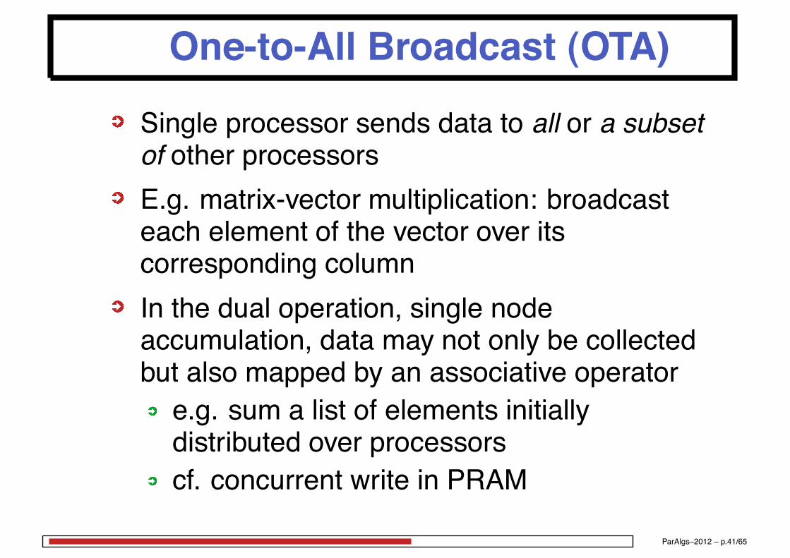
Single processor sends data to all or a subsetof other processorsE.g. matrix-vector multiplication: broadcasteach element of the vector over itscorresponding columnIn the dual operation, single nodeaccumulation, data may not only be collectedbut also mapped by an associative operatore.g. sum a list of elements initiallydistributed over processorscf. concurrent write in PRAM

ParAlgs–2012 – p.41/65

All-to-All Broadcast (ATA)

Each processor performs (simultaneously)one-to-all broadcast with its own dataUsed in matrix operations, e.g. matrixmultiplication, reduction and parallel-prefixIn the dual operation – multinodeaccumulation – each processor receivessingle-node accumulationCould implement ATA by sequentiallyperforming p OTAsFar better to proceed in parallel and catenateincoming data

ParAlgs–2012 – p.42/65

ReductionTo broadcast the reduction of the data held in allprocessors with an associative operator, we can:1. ATA broadcast the data and then reducelocally in every node . . . inefficient

2. Single node accumulation at one nodefollowed by OTA broadcast . . . better

3. Modify ATA broadcast so that instead ofcatenating messages, the incoming data andthe current accumulated value are operatedon by the associative operator – e.g. summed– the result overwriting the accumulated value..... the most efficient

ParAlgs–2012 – p.43/65

Parallel PrefixThe Parallel Prefix of a function f over anon-null list [x1, . . . , xn] is the list of reductionsof f over all sublists [x1, . . . , xi] for 1 ≤ i ≤ n,where reducef [x1] = x1 for all fCould implement as n reductionsBetter to modify the third reduction method byonly updating the accumulator at each nodewhen data comes in from the appropriatenodes (otherwise it is just passed on)

ParAlgs–2012 – p.44/65

All-to-All PersonalisedEvery processor sends a distinct message ofsize m to every other processor – ‘totalexchange’E.g. in matrix transpose, FFT, database joinCommunication patterns identical to ATALabel messages by pairs (x, y) where x is thesource processor and y is the destinationprocessor: uniquely determines the messagecontentsList of n messages denoted[(x1, y1), . . . , (xn, yn)]

ParAlgs–2012 – p.45/65

Performance Metrics1. Run Time, Tp

A parallel algorithm is hard to justifywithout improved run-timeTp = Elapsed time on p processors:between the start of computation on thefirst processor to start, and termination ofcomputation on the last processor to finish

ParAlgs–2012 – p.46/65

Performance Metrics (2)

2. Speed-up, Sp

Sp =serial run-time of “best” sequential algorithm

Tp

“best” algorithm is the optimal one for theproblem, if known, or the fastest known, ifnotoften in practice (always in this course) T1

Sp ≥ 1 . . . usually!

ParAlgs–2012 – p.47/65

Example – addition on hypercube

Add up p = 2d numbers on a d-hypercubeUse single node accumulationEach single-hop communication combinedwith one addition operation

⇒ Sp = Θ(p/ log p)

ParAlgs–2012 – p.48/65

Performance Metrics (2)

3. Efficiency, Ep

Ep =Sp

p

Fraction of time for which a processor isdoing useful workEp = Θ(1/ log p) in above example

ParAlgs–2012 – p.49/65

Performance Metrics (3)

4. Cost, Cp

Cp = p×Tp so that Ep =best serial run-time

Cp

A parallel algorithm is cost-optimal if Cp ∝best serial run timeEquivalently if Ep = Θ(1)

Above example is not cost-optimal sincebest serial run time is Θ(p)

ParAlgs–2012 – p.50/65

Granularity

“Amount of work allocated to each processor”Few processors, relatively large processingload on each⇒ coarse-grained parallelalgorithmMany processors, relatively small processingload on each⇒ fine-grained parallelalgorithme.g. our hypercube algorithm to add up pnumberstypically many small communications, oftenin parallel

ParAlgs–2012 – p.51/65

Increasing the granularity

Let each processor “simulate” k processors ina finer-grained parallel algorithmComputation at each processor increases bya factor k

Communication time increases by factor ≤ k

typically << k

but may have much larger message sizes,e.g. k parallel communications may map toa single communication k times bigger

Hence Tp/k ≤ k × Tp and so Cp/k ≤ Cp

Cost-optimality preserved – may be created?ParAlgs–2012 – p.52/65

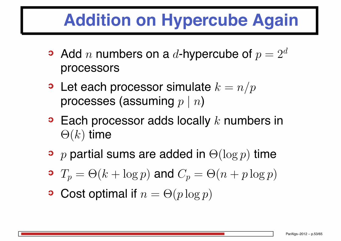
Addition on Hypercube Again

Add n numbers on a d-hypercube of p = 2d

processorsLet each processor simulate k = n/pprocesses (assuming p | n)Each processor adds locally k numbers inΘ(k) timep partial sums are added in Θ(log p) timeTp = Θ(k + log p) and Cp = Θ(n + p log p)

Cost optimal if n = Θ(p log p)

ParAlgs–2012 – p.53/65

Addition on Hypercube Again (2)

Alternatively, try communication in the first log psteps, followed by local addition of n/p numbers

Tp = Θ((n/p) log p)

So Cp = Θ((n) log p) = log p × Θ(C1)

never cost-optimal

ParAlgs–2012 – p.54/65

Scalability

Efficiency decreases as the number ofprocessors increasesConsequence of Amdahl’s Law:

Sp ≤problem size

size of serial part of problem

where size is the number of basic computationsteps in the best serial algorithm

ParAlgs–2012 – p.55/65

Scalability (2)

A parallel system is scalable if it can maintainthe efficiency of a parallel algorithm bysimultaneously increasing the number ofprocesors and problem sizeE.g. in the above example, efficiency remainsat 80% if n is increased with p as 8p log p

But you can’t tell me why yet!

ParAlgs–2012 – p.56/65

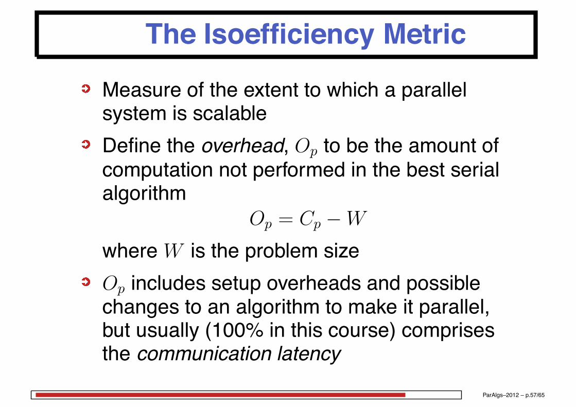
The Isoefficiency Metric

Measure of the extent to which a parallelsystem is scalableDefine the overhead, Op to be the amount ofcomputation not performed in the best serialalgorithm

Op = Cp − W

where W is the problem sizeOp includes setup overheads and possiblechanges to an algorithm to make it parallel,but usually (100% in this course) comprisesthe communication latency

ParAlgs–2012 – p.57/65

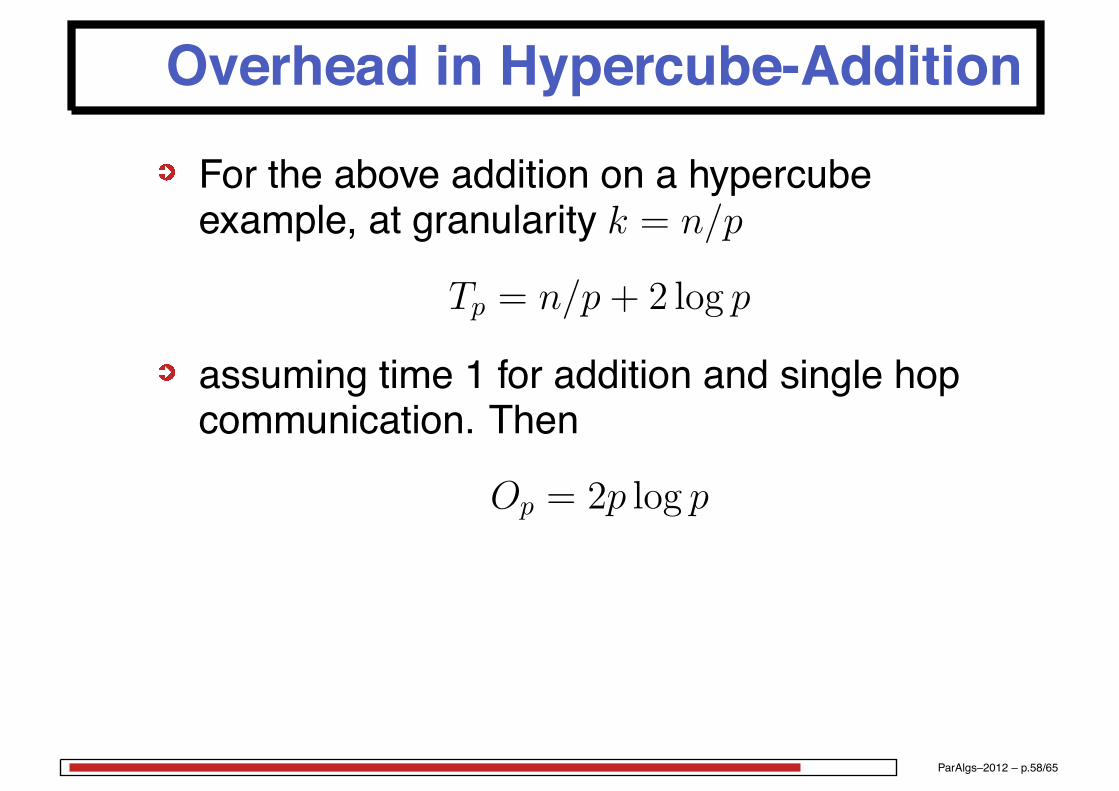
Overhead in Hypercube-Addition

For the above addition on a hypercubeexample, at granularity k = n/p

Tp = n/p + 2 log p

assuming time 1 for addition and single hopcommunication. Then

Op = 2p log p

ParAlgs–2012 – p.58/65

Isoefficiency

For a scalable system, the isoefficiencyfunction I determines W in terms of p and Esuch that efficiency, Ep, is fixed at somespecified constant value E

E = Sp/p = W/Cp

=W

W + Op(W )

=1

1 + Op(W )/W

ParAlgs–2012 – p.59/65

Isoefficiency (2)

Rearranging, 1 + Op(W )/W = 1/E, and so

W =E

1 − EOp(W )

This is the Isoefficiency EquationSetting K = E/(1 − E) for our given E, let thesolution of this equation (assuming it exists,i.e. for a scalable system) be W = I(p,K) –the Isoefficiency function

ParAlgs–2012 – p.60/65

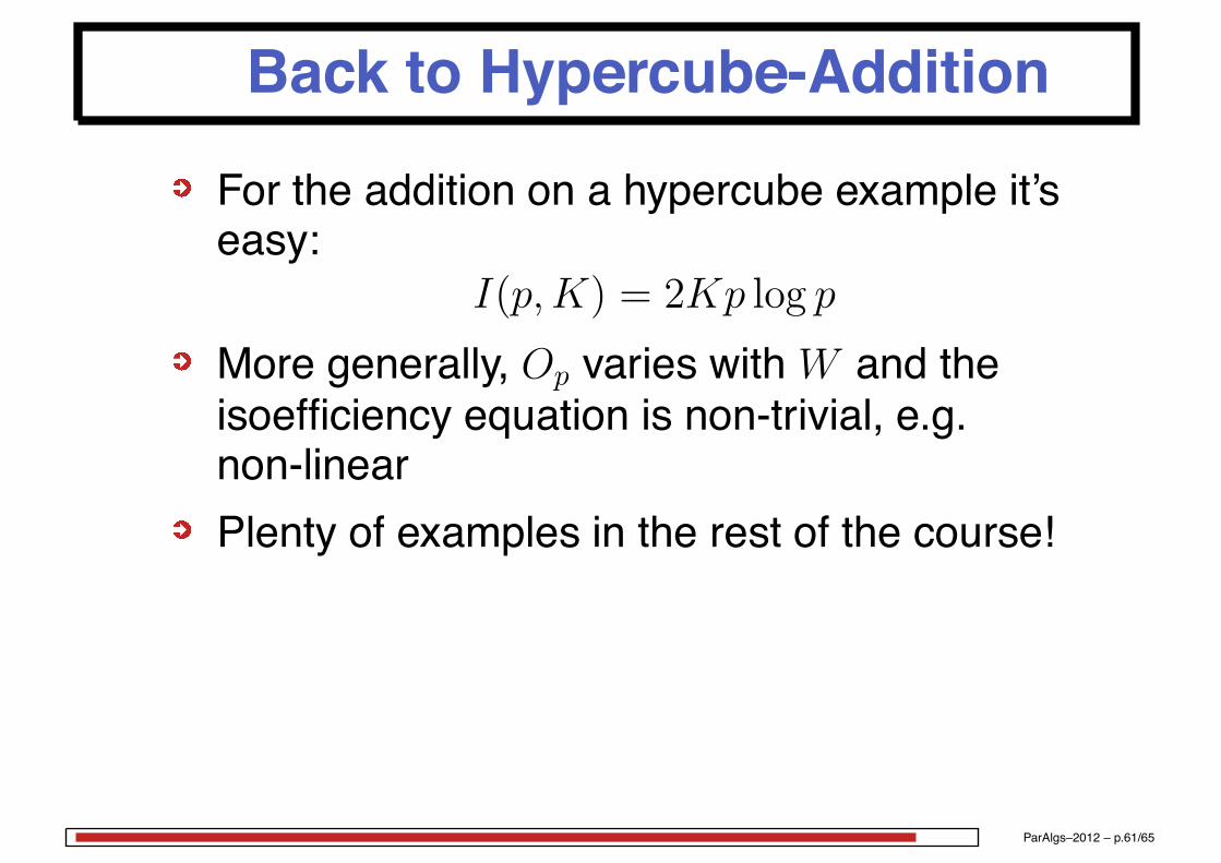
Back to Hypercube-Addition

For the addition on a hypercube example it’seasy:

I(p,K) = 2Kp log p

More generally, Op varies with W and theisoefficiency equation is non-trivial, e.g.non-linearPlenty of examples in the rest of the course!

ParAlgs–2012 – p.61/65

Cost-optimality and Isoefficiency

A parallel system is cost-optimal if and only ifCp = Θ(W ), i.e. its cost is asymptotically thesame as the cost of the serial algorithmThis implies the upper bound on the overhead

Op(W ) = O(W )

or lower bound on the problem size

W = Ω(Op(W ))

Not surprising – you don’t want a biggeroverhead than the computation of the solutionitself!

ParAlgs–2012 – p.62/65

Cost-optimality and Isoefficiency (2)

For the above example W = Θ(n) andOp(W ) = 2p log p so that the system cannot becost-optimal unless n = Ω(p log p)

the condition for cost-optimality alreadyderivedthe system is then scalable – its isoefficiencyfunction is Θ(p log p)

ParAlgs–2012 – p.63/65

Minimum Run-TimeAssuming differentiability of the expression forTp, find p = p0 such that

dTp

dp= 0

giving Tp = Tminp

For the above example,

Tp = n/p + 2 log p

p0 = n/2 ⇒ Tminp = 2 log n

Not cost-optimalParAlgs–2012 – p.64/65

Minimum Cost-Optimal Run-Time

For isoefficiency function Θ(f(p)) (at anyefficiency), W = Ω(f(p)) or p = O(f−1(W ))

Then minimum cost-optimal run time is

Tmin-cost-optp = Ω(W/f−1(W ))

For our example, n = f(p) = p log p and wefind p = f−1(n) = n/ log p + n/ log n so that

Tmin-cost-optp + 3 log n − 2 log log n

here, same asymptotic complexity as T minp

ParAlgs–2012 – p.65/65