parallel and multistep simulation of power system transients

POLYTECHNIQUE MONTRÉAL

affiliée à l’Université de Montréal

Parallel and multistep simulation of power system transients

MING CAI

Département de génie électrique

Thèse présentée en vue de l’obtention du diplôme de Philosophiæ Doctor

Génie électrique

Octobre 2019

© Ming Cai, 2019.

POLYTECHNIQUE MONTRÉAL

affiliée à l’Université de Montréal

Cette thèse intitulée :

Parallel and multistep simulation of power system transients

présentée par Ming CAI

en vue de l’obtention du diplôme de Philosophiæ Doctor

a été dûment acceptée par le jury d’examen constitué de :

Keyhan SHESHYEKANI, président

Jean MAHSEREDJIAN, membre et directeur de recherche

Ilhan KOCAR, membre et codirecteur de recherche

Houshang KARIMI, membre

Antonio Carlos Siqueira DE LIMA, membre externe

iii

DEDICATION

To all that came into my life and remain therein

iv

ACKNOWLEDGEMENTS

First and foremost, I would like to express my sincere gratitude to Dr. Jean Mahseredjian, my Ph.D.

director, for the opportunity he gave me to study at Polytechnique Montréal, as well as his patience,

advice and continuous support during the entire four years of my research. His work ethic and

comprehensive knowledge have greatly inspired and motivated me in my future career orientation.

I also owe my gratitude to Dr. Akihiro Ametani for his constant support, advice, encouragement,

and all the discussions we have had. Time spent with him has been a great joy in both my

professional and personal life.

I would like to thank Mr. Ali El-Akoum from Électricité de France (EDF) Lab Paris-Saclay and

Mr. Emmanuel Rutovic for the valuable discussions on the Functional Mock-up Interface (FMI)

standard.

Guidance, advice and help from Mr. Aboutaleb Haddadi are much appreciated.

Special thanks to all my colleagues, those who have already left and who will continue, for their

friendship and support: Isabel Lafaia, Baki Cetindag, Louis Filliot, Xiaopeng Fu, Fidji Diboune,

Serigne Seye, Thomas Kauffmann, Haoyan Xue, Anas Abusalah, Jesus Morales, Miguel Martinez,

Anton Stepanoz, Diane Desjardins, Reza Hassani, Masashi Natsui, David Tobar, Nazak

Soleimanpour, Willy Mimbe, and Aramis Trevisan. It was a great pleasure to have worked with

you.

Last but not least, to my parents who have always been there for me, I have no words but my

ultimate love and appreciation.

v

RÉSUMÉ

La simulation des régimes transitoires électromagnétiques (EMT) est devenue indispensable aux

ingénieurs dans de nombreuses études des réseaux électriques. L’approche EMT a une nature de

large bande et est applicable aux études des transitoires lents (électromécaniques) et rapides

(électromagnétiques). Cependant, la complexité des reseaux électriques modernes qui ne cesse de

s’accroître, particulièrement des réseaux avec des interconnexions HVDC et des éoliennes,

augmente considérablement le temps de résolution dans les études des transitoires

électromagnétiques qui exigent la résolution précise des systèmes d’équations différentielles et

algébriques avec un pas de calcul pré-déterminé. En tant que sujet de recherche, la réduction du

temps de résolution des grands réseaux électriques complexes a donc attiré beaucoup d’attention

et d’intérêt. Cette thèse a pour objectif de proposer de nouvelles méthodes numériques qui sont

efficaces, flexibles et précises pour la simulation des régimes transitoires électromagnétiques des

réseaux électriques.

Dans un premier temps, une approche parallèle et à pas multiples basée sur la norme Functional

Mock-up Interface (FMI) pour la simulation transitoire des réseaux électriques avec systèmes de

contrôle complexes est développée. La forme de co-simulation de la norme FMI dont l’objectif est

de faciliter l’échange de données entre des modèles développés avec différents logiciels est

implémentée dans EMTP. Tout en profitant de cette implémentation, les différents systèmes de

contrôle complexes peuvent être découplés du réseau principal en mémoire et résolus de façon

indépendante sur des processeurs séparés. Ils communiquent avec le reseau principal à travers une

interface de co-simulation pendant une simulation. Cette méthodologie non seulement réduit la

charge de calcul total sur un seul processeur, mais elle permet aussi de simuler les systèmes de

contrôle découplés de façon parallèle et à pas multiples. Deux modes de co-simulation sont

proposés dans la première étape du développement, qui sont les modes asynchrone et synchrone.

Dans le mode asynchrone, tous les systèmes de contrôle découplés (esclaves) sont simulés en

parallèle avec le réseau principal (maître) en utilisant un seul pas de calcul tandis que le mode

synchrone permet une simulation séquentielle en utilisant différents pas de calcul dans le maître et

les esclaves. La communication entre le maître et les esclaves est realisée et coordonée par des

fonctions qui implémentent le primitif de synchronisation de bas niveau sémaphore. Dans la

deuxième étape du développement, afin d’améliorer la méthodologie originale, un nouveau mode

asynchrone parallèle à pas multiples (parallel multistep asynchronous mode) et une procédure de

vi

correction de signaux sont proposés. Le premier combine les avantages numériques

(respectivement la simulation en parallèle et à pas multiples) des deux modes développés

précédemment et la seconde, basée sur l’extrapolation linéaire, sert à améliorer la précision de

simulation. Cette approche est testée sur différents benchmarks des réseaux électriques avec

systèmes de contrôle complexes tels que les contrôles éoliens et les relais de protection. Ses

avantages de pouvoir entretenir et améliorer la précision, accélérer la simulation temporelle tout en

étant évolutive et flexible sont démontrés par les résultats de simulation en comparaison avec ceux

obtenus des simulations EMT sur un seul processeur.

Dans un deuxième temps, une approche de parallélisation-dans-le-temps (parallel-in-time) basée

sur la technique parallèle de regroupement et permutation d’équations (equation grouping and

reordering technique, PEGR) pour la simulation transitoire des réseaux électriques est développée

dans la thèse. La proposition originale de la technique PEGR, formulée dans une forme d’état, a

pour objectif de réduire le nombre total de pas de calcul de façon logarithmique en regroupant et

permutant les équations du réseau à plusieurs points de calcul. L’approche de parallélisation-dans-

le-temps développée dans cette thèse est adaptée à l’analyse nodale modifiée augmentée (modified-

augmented-nodal analysis, MANA). Elle est implémentée en C++ avec l’API OpenMP

Multithreading pour la parallélisation de résolution en utilisant différents nombres de fils. Le

solveur linéaire hautement efficace à matrice creuse KLU est utilisé comme le solveur pour les

matrices de réseau. Certaines stratégies de programmation et solutions aux problèmes rencontrés

dans les simulations transitoires réalistes des réseaux électriques sont inclues dans le

développement de l’approche. Cette approche de parallélisation-dans-le-temps permet une

formulation flexible en regroupant les équations du réseau à différents nombres de points de calcul,

qui est ajustable par rapport au nombre de processeurs de l’ordinateur utilisé. Afin de valider la

précision et l’efficacité de l’approche développée, elle est testée sur des benchmarks réalistes des

réseaux électriques et d’autres construits avec de nombreuses répliques de ces mêmes benchmarks

représentant des réseaux électriques à plus grandes échelles. Les résultats obtenus de cette approche

démontrent qu’elle peut accélérer la simulation temporelle des réseaux électriques à différentes

échelles en utilisant différents nombres de processeurs parallèles, en comparaison avec la méthode

de résolution séquentielle traditionnelle.

Enfin, certains travaux futurs sont proposés dans le cadre du projet de cette thèse.

vii

ABSTRACT

The simulation of electromagnetic transients (EMT) has become indispensable to utility engineers

in a multitude of studies in power systems. The EMT approach is of wideband nature and applicable

to both slower electromechanical as well as faster electromagnetic transients. However, the ever-

growing complexity of modern-day power systems, especially those with HVDC interconnections

and wind generations, considerably increases computational time in EMT studies which require

the accurate solution of usually large sets of differential and algebraic equations (DAEs) with a

pre-determinded time-step. Therefore, computing time reduction for solving complex, practical

and large-scale power system networks has become a hot research topic. This thesis proposes new

fast, flexible and accurate numerical methods for the simulation of power system electromagnetic

transients.

As a first step in this thesis, a parallel and multistep approach based on the Functional Mock-up

Interface (FMI) standard for power system EMT simulations with complex control systems is

developed. The co-simulation form of the FMI standard, a tool independent interface standard

aiming to facilitate data exchange between dynamic models developed in different simulation

environments, is implemented in EMTP. Taking advantage of the compatibility established

between the FMI standard and EMTP, various computationally demanding control systems can be

decoupled from the power network in memory, solved independently on separate processors, and

communicate with the power network through a co-simulation interface during a simulation. This

not only reduces the total computation burden on a single processor, but also allows parallel and

multistep simulation for the decoupled control systems. Following a master-slave co-simulation

scheme (with the master representing the power network and the slaves denoting the decoupled

control systems), two co-simulation modes, which are respectively the asynchronous and

synchronous modes, are proposed in the first stage of the development. In the asynchronous mode,

all decoupled subsystems are simulated in parallel with a single numerical integration time-step

whereas the synchronous mode allows the use of different numerical time-steps in a sequential co-

simulation environment. The communication between master and slaves is coordinated by

functions employing the low-level synchronization primitive semaphore. The second stage of the

development improves the original methodology by proposing the parallel multistep asynchronous

mode that combines the advantages (parallel and multistep simulation) of the previously developed

two modes together and a linear extrapolation-based signal correction procedure for enhanced

viii

simulation accuracy. All developments in this approach are tested on realistic power system

benchmarks with complex control systems such as wind generator controls and protection relays.

The advantages of this approach in maintaining and improving accuracy, simulation speedup,

scalability as well as flexibility are demonstrated by simulation results in comparison to

conventional single-core-based EMT simulations.

Next, a parallel-in-time approach based on the parallel-in-time equation grouping and reordering

(PEGR) technique is developed in the thesis for power system EMT simulations. The original

proposition of the PEGR technique aims to logathrimically reduce the number of time-domain

solution steps by grouping network equations at several solution time-points together and taking

advantage of independency between certain solution steps found after a series of recursive row and

column reordering. The parallel-in-time approach developed in this thesis adapts the original

formulation of the PEGR technique into the modified-augmented-nodal analysis (MANA) from

state-space and is implemented using C++ with API OpenMP Multithreading for parallelization

using different numbers of threads. The highly efficient sparse linear solver KLU is used as the

network matrix solver. Several programming concerns and issues encountered in realistic power

system EMT simulations are also considered in the development of this approach. This parallel-in-

time approach allows flexible formulation in grouping the network equations at different numbers

of solution time-points, catering to the computing capacity (in terms of the number of logical

processors) of the PC used in the simulation. Realistic power system benchmarks as well as larger

networks constructed with multiple replicas of these benchmarks are used to test the accuracy and

efficiency of the proposed approach. Its capability of speeding up a time-domain simulation using

different numbers of parallel processors for power systems of different levels of complexity is

demonstrated through simulation results in comparison to the conventional stepwise solution

scheme.

Finally, several possible future developments based on the completed work proposed in the thesis

are presented.

ix

TABLE OF CONTENTS

DEDICATION .............................................................................................................................. III

ACKNOWLEDGEMENTS .......................................................................................................... IV

RÉSUMÉ ........................................................................................................................................ V

ABSTRACT ................................................................................................................................. VII

TABLE OF CONTENTS .............................................................................................................. IX

LIST OF TABLES ..................................................................................................................... XIV

LIST OF FIGURES .................................................................................................................... XVI

LIST OF SYMBOLS AND ABBREVIATIONS ........................................................................ XX

LIST OF APPENDICES ............................................................................................................ XXI

CHAPTER 1 INTRODUCTION ............................................................................................... 1

1.1 Motivation ........................................................................................................................ 1

1.1.1 Accelerating EMT simulations—numerical solution algorithms ................................. 1

1.1.1.1 Adoption of sparse matrix solvers ........................................................................ 2

1.1.1.2 Parallelization techniques ..................................................................................... 2

1.1.1.3 Hybrid techniques ................................................................................................ 4

1.1.1.4 Network equivalents and frequency adaptive methods ........................................ 5

1.1.2 Accelerating EMT simulations—multistep solution techniques .................................. 5

1.2 Contributions .................................................................................................................... 6

1.3 Thesis outline ................................................................................................................... 9

CHAPTER 2 A PARALLEL MULTISTEP APPROACH BASED ON FUNCTIONAL

MOCK-UP INTERFACE (FMI) ................................................................................................... 11

2.1 Implementation of FMI in EMTP .................................................................................. 11

2.1.1 Functional Mock-up Interface (FMI) standard ........................................................... 11

x

2.1.2 Functional Mock-up Unit (FMU) ............................................................................... 13

2.1.2.1 Node: fmiModelDescription .............................................................................. 14

2.1.2.2 Node: fmiModelDescription\CoSimulation ....................................................... 15

2.1.2.3 Node: fmiModelDescription\ModelVariables .................................................... 16

2.1.2.4 Node: fmiModelDescription\Implementation .................................................... 17

2.1.3 Implementation of FMI functions for co-simulation .................................................. 18

2.1.3.1 Implementation of functions in FMI2_Link_Master ......................................... 20

2.1.3.2 Implementation of functions in FMI2_Device_Master ...................................... 22

2.1.3.3 Implementation of functions in FMI2_Link_Slave and FMI2_Device_Slave ... 24

2.1.4 Function calling sequence in the master and slave programs .................................... 25

2.2 Co-simulation management ............................................................................................ 30

2.2.1 Synchronization between master and slaves .............................................................. 30

2.2.1.1 Semaphore management .................................................................................... 31

2.2.1.2 Master-slave synchronization: initialization mode ............................................ 33

2.2.1.3 Master-slave synchronization: synchronous mode (with a single numerical

integration time-step) ......................................................................................................... 34

2.2.1.4 Master-slave synchronization: asynchronous mode (with a single numerical

integration time-step) ......................................................................................................... 35

2.2.1.5 Master-slave synchronization: synchronous mode (with different numerical

integration time-steps) ........................................................................................................ 36

2.2.2 Data exchange between master and slaves ................................................................. 38

2.3 Improvements on the original methodology .................................................................. 40

2.3.1 Parallel multistep asynchronous mode ....................................................................... 40

2.3.2 Linear extrapolation-based signal correction ............................................................. 45

2.4 Conclusion ...................................................................................................................... 47

xi

CHAPTER 3 TEST CASES AND SIMULATION RESULTS OF THE FMI-BASED

APPROACH……………………………………………………………………………………...49

3.1 Validation of the co-simulation interface design ........................................................... 49

3.1.1 Creation of master and slave models .......................................................................... 49

3.1.2 Simulation results ....................................................................................................... 53

3.2 Validation of the original methodology ......................................................................... 56

3.2.1 Accuracy validation .................................................................................................... 56

3.2.1.1 Test case Network-1 ........................................................................................... 56


3.2.1.3 Error analysis ...................................................................................................... 68

3.2.2 Computation time gains ............................................................................................. 71


3.2.2.2 Test case Nework-2 ............................................................................................ 74

3.2.2.3 Discussion .......................................................................................................... 76

3.3 Validation of the improved methodology ...................................................................... 81

3.3.1 Accuracy validation—parallel multistep asynchronous mode ................................... 82

3.3.2 Accuracy validation—linear extrapolation-based signal correction .......................... 84



3.3.3 Computation time gains ............................................................................................. 93




3.3.3.4 Discussion .......................................................................................................... 97

3.4 Conclusion ...................................................................................................................... 98

xii

CHAPTER 4 A PARALLEL-IN-TIME APPROACH BASED ON PARALLEL-IN-TIME

EQUATION GROUPING AND REORDERING (PEGR) .......................................................... 99

4.1 Formulation of the PEGR technique in MANA ........................................................... 100

4.1.1 Modified-augmented-nodal analysis (MANA) ........................................................ 100

4.1.2 Expansion of network MANA equations ................................................................. 102

4.1.3 Grouping and recursive row and column reordering of expanded network MANA

equations ............................................................................................................................... 107

4.2 Implementation of the PEGR-based parallel-in-time approach ................................... 114

4.2.1 Parallelization using OpenMP .................................................................................. 115

4.2.2 Measures against false sharing, data race and inconsistency between temporary view

and memory .......................................................................................................................... 117

4.2.2.1 Minimizing false sharing .................................................................................. 117

4.2.2.2 Minimizing data race ........................................................................................ 118

4.2.2.3 Enforcing consistency between the temporary view and memory ................... 118

4.2.3 Block element extraction for forward and backward substitutions .......................... 119

4.2.4 Treatment of arbitrary points of topological changes and numbers of simulation

points………………………………………………………………………………………122

4.3 Conclusion .................................................................................................................... 124

CHAPTER 5 TEST CASES AND SIMULATION RESULTS OF THE PEGR-BASED

PARALLEL-IN-TIME APPROACH ......................................................................................... 126

5.1 Accuracy validation ...................................................................................................... 126

5.2 Computation time gains ............................................................................................... 129

5.2.1 Test case 1 ................................................................................................................ 129

5.2.2 Test case 2 ................................................................................................................ 130

5.2.3 Discussion ................................................................................................................ 132

xiii

5.3 Conclusion .................................................................................................................... 136

CHAPTER 6 CONCLUSION AND RECOMMENDATIONS ............................................ 137

6.1 Summary of the thesis .................................................................................................. 137

6.2 Future work .................................................................................................................. 140

BIBLIOGRAPHY ....................................................................................................................... 143

APPENDICES ............................................................................................................................. 154

xiv

LIST OF TABLES

Table 2.1 Attributes of node fmiModelDescription ...................................................................... 14

Table 2.2 Attributes of node fmiModelDescription\CoSimulation ............................................... 15

Table 2.3 Attributes of node fmiModelDescription\ModelVariable ............................................. 16

Table 2.4 Structure of the container InOut (co-simulation bus) ................................................... 39

Table 3.1 Co-simulation mode scenarios, co-simulation interface design validation ................... 54

Table 3.2 Co-simulation mode scenarios, accuracy validation of the original methodology,

Network-1 ............................................................................................................................... 57

Table 3.3 Relay 1 to 5 tripping zones ............................................................................................ 66


Network-2 ............................................................................................................................... 66

Table 3.5 Hardware and software configurations of the PCs ........................................................ 72

Table 3.6 Co-simulation mode scenarios, computation time gains ............................................... 72

Table 3.7 Comparison of solution times (s) on a PC with 2 cores (4 logical processors) for different

scenarios, Network-1 .............................................................................................................. 73

Table 3.8 Comparison of solution times (s) on a PC with 16 cores (32 logical processors) for

different scenarios, Network-1 ............................................................................................... 73


scenarios, Network-2 .............................................................................................................. 74


different scenarios, Network-2 ............................................................................................... 75

Table 3.11 Snippet of comparison of solution times (s) on a PC with 2 cores (4 logical processors)

for different scenarios, Network-2 ......................................................................................... 80

Table 3.12 Co-simulation mode scenarios, accuracy validation of the parallel multistep

asynchronous mode ................................................................................................................ 82

xv

Table 3.13 Co-simulation mode scenarios, accuracy validation of the linear extrapolation-based

signal correction procedure, Network-3 ................................................................................. 84


signal correction procedure, Network-4 ................................................................................. 89

Table 3.15 Co-simulation mode scenarios, computation time gains with the parallel multistep

asynchronous mode, Network-1 and -2 .................................................................................. 93

Table 3.16 Comparison of solution times (s) on the PC with 16 cores for different scenarios,

Network-1, improved methodology ....................................................................................... 94


Network-2, improved methodology ....................................................................................... 95

Table 3.18 Hardware and software configurations of the 24-core PC .......................................... 96


asynchronous mode, Network-4 ............................................................................................. 96

Table 3.20 Comparison of solution times (s) on the PC with 24 cores (48 logical processors) for

different scenarios, Network-4, improved methodology ....................................................... 97

Table 5.1 Performance timings of test case 1 .............................................................................. 130

Table 5.2 Performance timings of test case 2 .............................................................................. 132

xvi

LIST OF FIGURES

Figure 2.1 FMI for model exchange .............................................................................................. 12

Figure 2.2 FMI for co-simulation .................................................................................................. 13

Figure 2.3 Interfacing three subnetworks (Master, Slave 1 and Slave 2) via DLL files and two co-

simulation buses ..................................................................................................................... 19

Figure 2.4 One possible implementation of the master program of co-simulation of an UML 2.0

state machine .......................................................................................................................... 27

Figure 2.5 Principal function calling sequence in the master algorithm ....................................... 28

Figure 2.6 Principal function calling sequence in the slave algorithm ......................................... 29

Figure 2.7 Synchronization scheme between master and slave during initialization stage .......... 34

Figure 2.8 Synchronization scheme between master and slave in synchronous mode (with a single

numerical integration time-step) ............................................................................................ 35

Figure 2.9 Synchronization scheme between master and slave in asynchronous mode (with a single

numerical integration time-step) ............................................................................................ 36

Figure 2.10 Function fmi2DoStep in synchronous mode (with different numerical integration time-

steps) ....................................................................................................................................... 37

Figure 2.11 Synchronization scheme between master and slave in synchronous mode ............... 37

Figure 2.12 Synchronization scheme between master and slave in the improved asynchronous

mode (parallel multistep asynchronous mode) ....................................................................... 41

Figure 2.13 First synchronization scenario ( master slavet t∆ = ∆ ) between master and slave in the

parallel multistep asynchronous mode ................................................................................... 42

Figure 2.14 Second synchronization scenario ( master slavet t∆ < ∆ ) between master and slave in the


Figure 2.15 Third synchronization scenario ( master slavet t∆ > ∆ ) between master and slave in the


Figure 3.1 Test circuit for the validation of co-simulation interface design ................................. 50

xvii

Figure 3.2 Slave subsystem for the validation of co-simulation interface design ......................... 50

Figure 3.3 Inputs and outputs settings in the slave ....................................................................... 51

Figure 3.4 Co-simulation mode and other parameter settings in the slave ................................... 51

Figure 3.5 Master subsystem for the validation of co-simulation interface design ...................... 52

Figure 3.6 Loaded data and parameters from the slave FMU in the master ................................. 53

Figure 3.7 Waveforms of Output 1 for all simulation scenarios ................................................... 54

Figure 3.8 Waveforms of Output 2 for all simulation scenarios ................................................... 55

Figure 3.9 Closer observation of waveform of Output 2 for all simulation scenarios .................. 55

Figure 3.10 Network-1 benchmark ............................................................................................... 58

Figure 3.11 Offshore wind parks and HVDC connection in Network-1 ...................................... 59

Figure 3.12 Design of one offshore wind park in Network-1 ....................................................... 59

Figure 3.13 DFIG model in the offshore wind parks in Network-1 .............................................. 60

Figure 3.14 Control system design for the DFIG model in the offshore wind parks .................... 60

Figure 3.15 Waveforms of average active power and phase-a current ......................................... 61

Figure 3.16 Line relay at each end of a CP line ............................................................................ 62

Figure 3.17 Relay 1 settings (partial) ............................................................................................ 64


Figure 3.19 Tripping instants of Relays 1, 2 and 4 ....................................................................... 67

Figure 3.20 Phase a locus of Relay 1 ............................................................................................ 68

Figure 3.21 Simplified co-simulation process of Scenario 1 ........................................................ 69

Figure 3.22 Simplified co-simulation process of Scenario 3 ........................................................ 70

Figure 3.23 Total solution time speedup with respect to the number of slaves in Network-1 on a

PC with 2 cores (4 logical processors) ................................................................................... 73


PC with 16 cores (32 logical processors) ............................................................................... 74

xviii


PC with 2 cores (4 logical processors) ................................................................................... 75


PC with 16 cores (32 logical processors) ............................................................................... 75

Figure 3.27 Solution scheme in the original approach (EMTP) for the computation of one time-

step. ........................................................................................................................................ 77

Figure 3.28 Solution scheme using the FMI-based co-simulation approach (parallel asynchronous

mode) for the computation of one time-step. ......................................................................... 78

Figure 3.29 Tripping instants of Relays 1, 2 and 4 ....................................................................... 83


Figure 3.31 Phase-b voltage at bus XFMR between 0.5t s= and 0.55t s= without signal

correction with closer observation of waveforms in the amplified region ............................. 86

Figure 3.32 Phase-b voltage at bus XFMR between 0.5t s= and 0.55t s= with signal correction

with closer observation of waveforms in the amplified region .............................................. 87


Figure 3.34 Design of the F1 wind park feeder ............................................................................. 90

Figure 3.35 DFIG model with wind generator control systems modelled using the detailed model

................................................................................................................................................ 91

Figure 3.36 Control system design for the DFIG model in the wind generator ............................ 91

Figure 3.37 Average active power from wind park feeders .......................................................... 92

Figure 3.38 Phase-a voltage at the 34.5 kV bus ............................................................................ 92


16-core PC, improved methodology ...................................................................................... 94





xix

Figure 4.1 Multiphase pi-section schematic ................................................................................ 103

Figure 4.2 Expanded network equations incorporating current history terms into the vector of

unknowns, demonstrating interdependency of solutions at adjacent time-points ................ 104

Figure 4.3 Lower triangular matrix L and equations for forward substitution after a one-time row

and column reordering and LU factorization ....................................................................... 110

Figure 4.4 Lower triangular matrix L and equations for forward substitution after recursive row

and column reordering and LU factorization ....................................................................... 111

Figure 4.5 : Structure of the L and U factors when grouping the network equations of 16 time-steps

.............................................................................................................................................. 120

Figure 4.6 Switching between the PEGR-based approach and the conventional approach in the

case of topological changes in the network .......................................................................... 123


Figure 5.2 Phase-a fault current, phase-a voltages at buses 888 and 854 ................................... 128

Figure 5.3 Solution time speedup using the PEGR-based parallel-in-time approach with respect to

the number of launched threads in the simulation for test case 1 ........................................ 130


Figure 5.5 Solution time speedup using the PEGR-based parallel-in-time approach with respect to

the number of launched threads in the simulation for test case 2 ........................................ 132

xx

LIST OF SYMBOLS AND ABBREVIATIONS

DAE Differential and algebraic equation

DLL Dynamic-link library

EMT Electromagnetic transients

EMTP Electromagnetic transients program

FA Frequency adaptive

FDNE Frequency-dependent network equivalent

FMI Functional Mock-up Interface

FMU Functional Mock-up Unit

FPGA Field-programmable gate array

GPU Graphics processing unit

HVDC High voltage direct current

MANA Modified-augmented-nodal analysis

PEGR Parallel-in-time equation grouping and reordering

TS Transient stability

xxi

LIST OF APPENDICES

Appendix A – Example xml file in an Functional Mock-up Unit (FMU) ................................... 154

Appendix B – Detailed implementation of funcitons coordinating master-slave co-simulation . 159

Appendix C – Algorithm for the extraction of block elements in the L and U factors ................ 167

Appendix D – List of publications ............................................................................................... 172

1

CHAPTER 1 INTRODUCTION

1.1 Motivation

Modern-day power systems are increasingly complex, thanks to more and more challenging cases

created by state-of-the-art developments in the research fields such as HVDC systems and wind

generation [1]. Such ever-growing complexity of modern power grids requires high-performance

computing resources (preferably inexpensive) as well as advanced computer-based simulation

methods for design, operation and post-mortem analysis stages.

Numerical solution methods are crucial in the evolution and technological advancements in modern

power systems, in which circuit-based numerical methods, such as those used in the high accuracy

time-domain electromagnetic transients (EMT) simulations, are of particular interest to researchers

and utility engineers. The EMT approach [2]-[6] targets operation problems in power system

analyses. It helps utility engineers perform highly accurate studies including fault analysis, power

flow analysis, stability analysis as well as EMT analysis, demonstrating great advantages over

phasor-domain approaches [7], [8]. It is of wideband nature and applicable to both slower

electromechanical transients of lower frequencies as well as high frequency electromagnetic

transients, such as switching and lightning. Typical numerical integration time-steps are in the

range of µs, which creates major obstacles in terms of computing times in the accurate solution of

large sets of differential and algebraic equations (DAE) for large-scale systems. Therefore,

computing time reduction for solving complex, practical and large-scale power system networks

has become a hot research topic.

1.1.1 Accelerating EMT simulations—numerical solution algorithms

Over the years, many efforts have been dedicated to reducing computing times in EMT-type

simulation methods, in which development of models and new numerical solution algorithms have

drawn a fair amount of interest among researchers. The modelling aspect focuses mainly on

enhancing computational performance and optimizing accuracy for a given numerical integration

time-step in the implementation of model equations [9], [10]. Although this could, in some cases,

allow the adoption of larger numerical integration time-steps to improve simulation efficiency,

properly maintaining the accuracy, generalization and application in large-scale networks need to

2

be further investigated. Therefore, more efforts have been dedicated to the research on numerical

solution algorithms for enhancing the performance of EMT-type solution schemes, which fall

principally into the following categories: adoption of sparse matrix solvers, parallelization

techniques, hybrid techniques, network equivalents and frequency adaptive methods.

1.1.1.1 Adoption of sparse matrix solvers

Among all the available sparse linear solvers for efficient large sparse matrix solutions, LU

factorization is a popular approach and is used as a direct solver in circuit simulation [11]. In

particular, a Gilbert-Peierls’ left-looking algorithm based sparse high-performance linear solver

named KLU stands out in the solution of circuit matrices thanks to the efficient ordering

mechanisms and high-performance factorization and solve algorithms it adopts [12], [13].

Moreover, KLU uses a hybrid ordering strategy consisting of an unsymmetrical permutation to

ensure a zero-free diagonal, a symmetrical permutation to Block Triangular Form (BTF) and a fill-

in reducing ordering scheme to achieve a superior fill-in quality and good performance speedup

when compared to other existing sparse linear solvers for circuit simulation [12], [13]. A KLU-

based simulator developed in [13] has demonstrated its numerical advantages for solving circuit

matrices. Other LU factorization-based software packages can be found in [11].

1.1.1.2 Parallelization techniques

Parallelization is another area that has been researched in depth in computing time reduction.

Throughout the years, a great number of techniques and methods have been proposed and

developed in which parallelization is achieved by partitioning a network using the intrinsic

propagation delay at distributed parameter transmission line and cable models for natural

decoupling of networks while adopting a shared-memory computing scheme [14]-[18]. It is worth

mentioning that the co-simulation based parallel approach proposed in [16] partially implemented

the Functional Mock-up Interface (FMI) standard [19] with the adoption of a master-slave co-

simulation scheme. Notwithstanding, the steady-state solution needs to be obtained at the master-

slave interface and stored prior to each co-simulation start, and several steps in [16] are also

complex to automate and require user intervention. Other implementation of the co-simulation

approach in power system studies can be found in [20], [21].

3

Several more flexible partitioning techniques are also proposed in the literature, such as the state-

space nodal method in [22] and techniques based on the Multi-Area Thevenin Equivalents (MATE)

[23]-[27]. However, the MATE-based techniques can be related to more fundamental circuit

analysis theories, such as diakoptics [28], hybrid analysis [29] as well as the compensation method

to solve non-linearities using network decoupling in EMT-type solvers [29].

Compared to more commonly seen network decoupling based parallel-in-space approaches,

parallel-in-time approaches have not been widely researched due to the difficulty in identifying the

intrinsic independency of solutions at different time-steps. A parallel-in-time technique is proposed

in [30] that identifies truly independent tasks which could be performed simultaneously with an

ideal number of parallel processors after certain pre-processing procedures consisting of the

building of a huge matrix containing the solutions at all time-steps as well as a series of recursive

row and column reordering.

Additionally, an iterative method named waveform relaxation in which parallelism can be

exploited in space and time through partitioning is reported in [31]-[37]. Even though it has seen

applications in large-scale integrated circuits [32],[34] and transient stability analysis [35], its

feasibility and reliability in power system EMT simulations need to be further investigated.

Continuously stable developments in the semiconductor industry and advances in architecture

design have prompted the use of computational accelerators in order to enable higher performance

when exploiting fine-grained parallelism. The most popular accelerators are Field Programmable

Gate Arrays (FPGA) and graphical processing units (GPUs). Since nowadays new generations of

FPGAs have the ability of integrating a great number of computational modules and built-in

parallel machines, in recent years many attempts have been taken in exploring the parallel-in-space

characteristic of this promising computing paradigm [38]-[41]. On the other hand, many efforts

have been put in developing massive-threading CPU-GPU based and entirely GPU based fine-

grained parallel simulation approaches using the parallel computing platform and API CUDA

created by NVIDIA, as can be seen in [42]-[47]. These hardware accelerators can provide fast

computations for certain classes of problems and are used as an alternative to accelerate the circuit

simulation besides distributed and shared memory architectures.

Furthermore, multithreading can also be used to express parallelism in simulation programs on

shared-memory systems, in which OpenMP has become an industry standard API. An OpenMP

4

Multithreading based parallelization technique on multi-core systems is reported in [17], [18] for

the simulation of large power grids, with the network partitioned at distributed parameter

transmission lines, as was discussed earlier.

Apart from what has been discussed so far, the development of high-performance real-time EMT-

type simulation tools sparked a great deal of interest in the 1970s and has since become an

important research field in power system EMT simulations. Major achievements in the past few

decades are presented in [48]-[54], which include notably the full-digital real-time simulator

Hypersim [48], RTDS [50], a cluster-based real-time simulator [51] from the University of British

Columbia, and the processor cluster based real-time simulator eMEGAsim [52]. The basic principle

in real-time solvers is the separation of network equations onto several processing units through

the natural time-delay decoupling introduced by distributed parameter transmission line and cable

models. Despite their rising popularity in the industry, off-line simulators are still preferred for

their advantages in accuracy and ability of solving networks without dimension and numerical

integration time-step limits.

1.1.1.3 Hybrid techniques

Hybrid simulation techniques, the combination of an EMT-type algorithm simulating a section of

the network in detail whose dynamics are of crucial importance and a fundamental-frequency-

single-phase-based transient stability program (TS) for the rest of the network, have been

extensively studied in the literature [55]-[73]. It was originally proposed to achieve the simulation

speed of a TS-type solver that uses numerical integration time-steps in the order of milliseconds

while maintaining similar accuracy of an EMT-type solver that usually requires a much smaller

numerical integration time-step. Therefore, the conventional hybrid simulation approaches are

usually comprised of time-domain solution using the EMT-type solver and phase-domain solution

using the TS-type solver, associated through the choice of interface location, equivalencing of

different sections of the network, data conversion methods between time- and phasor-domain as

well as interaction protocol. Although such an approach can gain from the high efficiency of TS-

type solvers, the lack of concrete theoretical foundation, insufficient generalization and accuracy

control to deal with arbitrary network topologies prevent the hybrid simulation approaches from

gaining widespread applications in practice.

5

1.1.1.4 Network equivalents and frequency adaptive methods

Research on computing time reduction in frequency-domain is comprised chiefly of the use of

frequency dependent network equivalents (FDNEs) [74]-[76] and frequency adaptive (FA)

approaches [77], [78]. The former can be used to reduce the size of studied network and

consequently accelerate computations of localized transients, whereas the latter allows accelerating

computations by applying large time-steps when required for letting EMT-type methods to

efficiently perform TS-type computations. Nevertheless, the FDNE-based approaches are currently

limited to linear networks, and the selection of network equivalent ports calls for user intervention

and empirical judgement. Limitations of the FA-based techniques include higher computational

complexity compared to EMT-type approaches and possible errors brought by the aliasing effect

when simulating very fast transients.

1.1.2 Accelerating EMT simulations—multistep solution techniques

Another aspect of computing time reduction is the employment of multiple time-steps in different

subsystems of the network in the same simulation environment. This multistep simulation scheme,

similar to the conventional hybrid simulation approaches, is based on the generalized relaxation

technique in which subsystems employing smaller numerical integration time-steps are solved

independently while considering those with a larger numerical integration time-step remain

unchanged. Solutions are consequently interfaced and updated at the interfacing locations at certain

fixed time-points. Using such a simulation scheme, a “data-smoothing” technique at line-bus

interfaces is proposed in [79], and a frequency-domain multistep approach is proposed in [80].

Although computational speedup has been observed in some cases, the implementation of such

multistep techniques on large-scale networks requires user intervention and remains complex to

automate [81].

On a side note, currently all EMT-type solvers for large power system simulations are based on the

fixed time-step trapezoidal integration methods. Variable time-step numerical integration methods

for the solution of differential equations have seen applications in SPICE tools. Notwithstanding

that overall improved numerical performance can be expected with these methods, step size

management for better accuracy control arises as a complex problem [82], [83]. In particular, two

time-step control mechanisms, iteration-count time-step control and truncation-error time-step

control, for variable time-step numerical integration methods were discussed in [82]. It is

6

demonstrated that the former control mechanism exhibits problems in solution errors, whereas the

latter has issues in simulation efficiency with certain types of circuits. Overall, both control

mechanisms are circuit-dependent and require a certain level of intervention and empirical

judgement from the user.

This thesis is focused on the design and implementation of novel parallel and multistep numerical

techniques based on the current network partitioning, generalized relaxation and co-simulation

paradigms for fast large-scale power system EMT simulations while accurately accounting for

various dynamic phenomena. Parallelism in the developed techniques is exploited both in space

and in time. The newly developed techniques are either implemented directly on an EMT-type

solver [2] or in an EMT solution scheme. Unique advantages of these techniques in terms of

efficiency, flexibility, scalability, level of automation and accuracy control are demonstrated

through tests results on power system benchmarks of different levels of complexity, in comparison

to conventional EMT-type solution methods.

1.2 Contributions

The achievements and contributions of this thesis are summarized here.

IMPLEMENTATION OF THE FUNCTIONAL MOCK-UP INTERFACE (FMI)

STANDARD IN EMTP

The Functional Mock-up Interface (FMI) standard is a tool independent interface standard

developed in the context of the European project Modelisar, providing support for standardized

data exchange between dynamic models designed under different simulation environments with

the help of xml files and C-code [19]. It aims at exchanging dynamic models between tools with

ease, obviating the need to convert one dynamic model developed in a different simulation tool to

one adapted to the host simulation tool, and providing an interface standard for coupling of

simulation tools in a co-simulation environment. The FMI standard comes in two forms: model

exchange and co-simulation. In this thesis, the co-simulation form of the FMI standard is fully

implemented in an EMT-type solver [2] and all FMI functions are concretized for the purpose of

power system EMT simulations, particularly for power grids with control systems while respecting

standard simulation procedure defined in the standard [19]. Such an implementation remarkedly

7

enhances the flexibility of power system EMT-type solvers in their ability of accommodating a

broad range of dynamic simulation needs and environments and presents great prospects for

parallel and distributed computation by exploiting the modular nature of decoupled dynamic

models.

DEVELOPMENT OF A NEW OFF-LINE SIMULATION METHOD BASED ON THE

CO-SIMULATION APPROACH AND USING THE FMI STANDARD FOR

PARALLEL AND MULTISTEP EMT SIMULATIONS WITH CONTROL SYSTEMS

One contribution in this thesis is the design and implementation of a new off-line parallel and

multistep simulation method based on the co-simulation approach using the FMI standard for

power system EMT simulations with control systems on conventional multicore computers. Instead

of bridging different solvers, this newly developed approach interfaces different instances of the

same solver using decoupling in memory between power network and control systems in which

the control systems are decoupled from the power networks into subsystems and the calculation of

all subsystems are distributed among separate processors.

The development of this new approach is realized in two stages. In the first stage, full compatibility

between EMTP and the FMI standard is established, a master-slave co-simulation scheme is

adopted with the master representing the power network and the slaves denoting the decoupled

control systems, and two co-simulation modes are designed (asynchronous and synchronous). In

the asynchronous mode, the decoupled subsystems are simulated in parallel using a single

numerical integration time-step, whereas in the synchronous mode the simulation of each

subsystem is executed in a sequential multistep environment. Considerable computational speedup

in both modes is observed in power system protection studies on large-scale networks with

accuracy properly maintained.

In the second stage, the computational capacity of the asynchronous mode is extended into

accommodating the use of different numerical integration time-steps in different subsystems

decoupled in memory, greatly improving simulation flexibility and efficiency. Furthermore, a

signal correction procedure based on linear extrapolation is introduced to achieve higher accuracy

in a multistep simulation environment.

The developed off-line parallel and multistep EMT simulation approach, with its complete memory

decoupling between power network and control systems, pure EMT nature, EMT accuracy and

8

targeted decoupling interface, presents great prospects of higher simulation scalability, flexibility

and level of automation in the massive use of control diagram blocks in power system simulations.

Unique advantages are demonstrated for large protection system studies.

DEVELOPMENT OF A NEW OFF-LINE PARALLEL-IN-TIME APPROACH BASED

ON THE PARALLEL-IN-TIME EQUATION GROUPING AND REORDERING (PEGR)

TECHNIQUE FOR POWER SYSTEM EMT SIMULATIONS

Another contribution in this thesis is the development of a new parallel-in-time off-line approach

based on the parallel-in-time equation grouping and reordering (PEGR) technique for power system

EMT simulations. In the development of this new approach, the fundamental theories of the PEGR

technique are revisited, and its original formulation in state-space is extended to the later more

popular and advantageous modified-augmented-nodal analysis (MANA) formulation method [2].

This approach concretizes the PEGR technique to constructing a large DAE system that

incorporates the solutions at multiple time-points, thereby logarithmically reducing the actual

number of solution steps in the forward and backward substitution procedures with the help of

recursive row and column reordering.

The algorithm of this approach is realized in C++ with API OpenMP Multithreading, catering to

the current computing capability of most off-the-shelf PCs, and the highly efficient sparse linear

solver KLU is used as the network matrix solver. Measures are taken to tackle concurrency issues

encountered in a parallel computing environment. Treatment of topological changes and arbitrary

numbers of simulation points is also included in the algorithm. It is worth mentioning that the

developed parallel-in-time approach offers flexible formulation of grouping the network equations

at various solution time-points, suitable for PCs with any number of logical processors to attain

their full potential of parallelism.

This newly developed parallel-in-time approach, due to its special network equation formulation

scheme that differs significantly from the conventional EMT step-wise approaches, sheds

remarkable insight on fast power system EMT simulation from a different perspective. It serves as

a prototype in a new parallel simulation scheme and facilitates possible integration with other

techniques (e.g., hybrid techniques) to solve for power system dynamic problems on a much larger

scale.

9

1.3 Thesis outline

This thesis is composed of six chapters and four appendices.

CHAPTER 1 INTRODUCTION

This chapter explains the background motivating this PhD project, highlights its objectives and

contributions and summarizes the contents of each chapter.

CHAPTER 2 A PARALLEL MULTISTEP APPROACH BASED ON FUNCTIONAL

MOCK-UP INTERFACE (FMI)

It presents the details of implementation of the Functional Mock-up Interface (FMI) standard in

EMTP. This includes the adoption of a master-slave co-simulation scheme, the design of two co-

simulation modes (parallel single-step asynchronous and sequential multistep synchronous), and

the master-slave synchronization process in both modes with the use of low-level synchronization

primitive semaphore. Two improvements on the original methodology are then introduced: the

development of the parallel multistep asynchronous mode and the linear extrapolation-based signal

correction procedure.

CHAPTER 3 TEST CASES AND SIMULATION RESULTS OF THE FMI-BASED

APPROACH

This chapter contains simulation results using the approach developed in Chapter 2 on power

system benchmarks of different levels of complexity, compared with those obtained from a

conventional EMT-type solver. Error analysis for the accuracy validation tests and discussion on

the observed computational speedup are also provided.

CHAPTER 4 A PARALLEL-IN-TIME APPROACH BASED ON PARALLEL-IN-TIME

EQUATION GROUPING AND REORDERING (PEGR)

The development of the off-line parallel-in-time approach based on the PEGR technique is

explained in detail in this chapter. It starts off with the theoretical background of the modified

augmented nodal analysis (MANA) and the PEGR technique, then moves on to the adaptation of

the PEGR technique from state-space to MANA formulation, its implementation in C++ with

OpenMP Multithreading. Detailed programming consideration to minimize concurrency issues as

10

well as the treatment of topological changes and arbitrary numbers of simulation points are also

elaborated.

CHAPTER 5 TEST CASES AND SIMULATION RESULTS OF THE PEGR-BASED

PARALLEL-IN-TIME APPROACH

This chapter presents simulation results of the parallel-in-time approach developed in Chapter 4 on

various test cases using different numbers of threads, compared to those obtained from the

conventional EMT-type step-wise solution scheme.

CHAPTER 6 CONCLUSION

The main conclusions of the thesis and possible future developments based on this work are

presented in this chapter.

APPENDIX A EXAMPLE XML FILE IN AN FUNCTIONAL MOCK-UP UNIT (FMU)

An example xml file in an FMU generated from a wind generator control system is presented in

this appendix.

APPENDIX B DETAILED IMPLEMENTATION OF FUNCITONS COORDINATING

MASTER-SLAVE CO-SIMULATION

This appendix presents detailed implementation of functions used in the master-slave

communication and data exchange process.

APPENDIX C ALGORITHM FOR THE EXTRACTION OF BLOCK ELEMENTS IN

THE L AND U FACTORS

The algorithm to extract various block elements in the L and U factors for forward and backward

substitutions in the PEGR-based parallel-in-time approach is presented in this appendix.

APPENDIX D LIST OF PUBLICATIONS

All journal and conference publications derived from the work of this thesis are presented here.

11

CHAPTER 2 A PARALLEL MULTISTEP APPROACH BASED ON

FUNCTIONAL MOCK-UP INTERFACE (FMI)

In this chapter, the implementation of the FMI standard in EMTP is explained in detail with

elaboration on the contents and functionalities of the executable Functional Mock-up Unit (FMU)

as well as the concretization of the FMI functions in the context of co-simulation. It proceeds with

co-simulation management including the adoption of a master-slave co-simulation scheme, the

design of different co-simulation modes, synchronization and data exchange between master and

slaves. Two improvements on such a methodology are then proposed for the enhancement of

simulation flexibility, efficiency and accuracy.

2.1 Implementation of FMI in EMTP

This section provides a brief introduction on the FMI standard (more details can be found in [19]),

with focus on the definition and components of the executable FMU implementing the interface

defined by the standard and detailed implementation of FMI functions for co-simulation.

2.1.1 Functional Mock-up Interface (FMI) standard

As was mentioned in Chapter 1, the Functional Mock-up Interface (FMI) standard is a tool

independent interface standard developed in the context of the European project Modelisar,

providing support for standardized data exchange between dynamic models designed under

different simulation environments with the help of a combination of xml files and C-code (either

compiled in DLL/shared libraries or in source code). The first version, FMI 1.0, was finalized and

published in 2010, and the design of the second version, FMI 2.0, came into fruition in 2014. The

standard is freely accessible under the licence CC-BY-SA [84].

A number of potential advantages prompted the development of such a standard:

• Firstly, it obviates the need to convert a dynamic model developed in a different simulation

tool to one adapted to the host simulation tool as details of such a model, usually enclosed

in a “blackbox”, are often unknown to the user.

• Secondly, a co-simulation can be easily launched without having to generate DLL code or

using a third-party software.

12

• Thirdly, the exploitation of the modular nature of dynamic models and co-simulation slaves

shows great prospects for parallel and distributed computation.

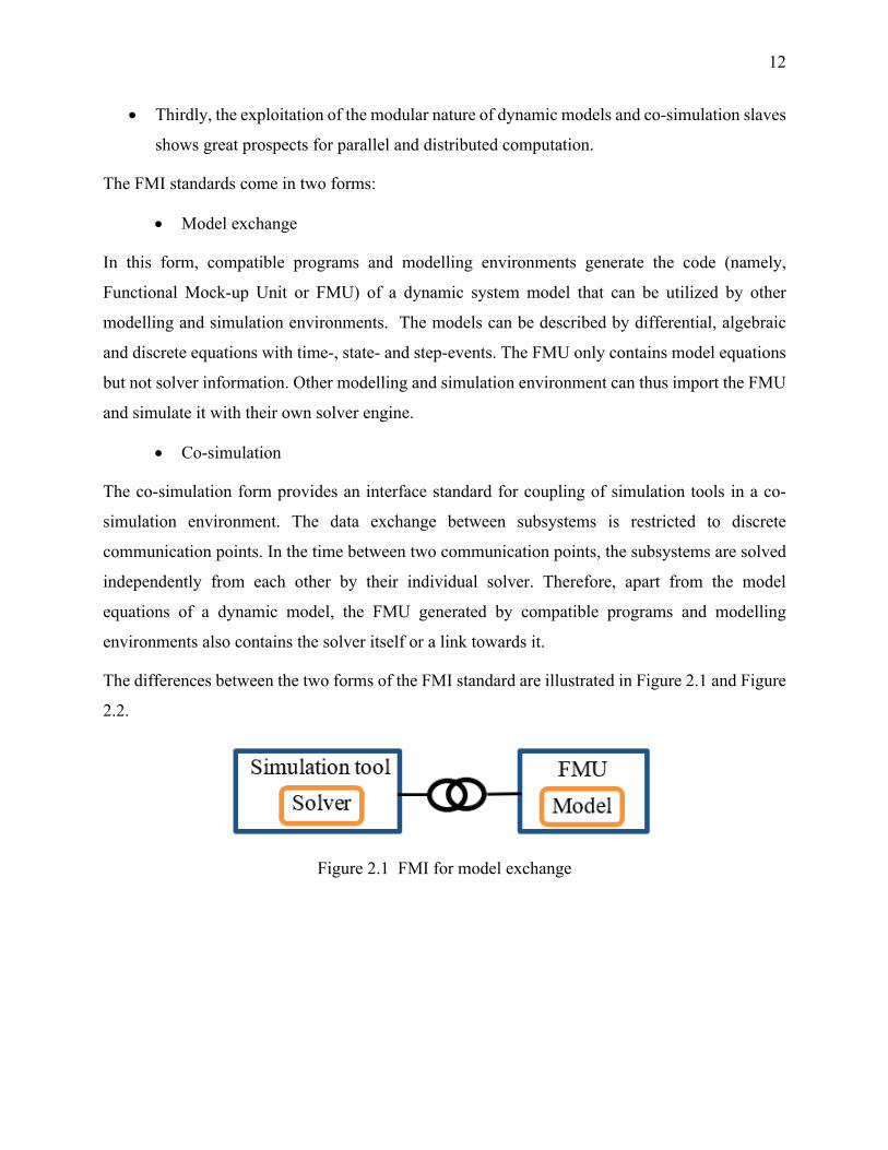
The FMI standards come in two forms:

• Model exchange

In this form, compatible programs and modelling environments generate the code (namely,

Functional Mock-up Unit or FMU) of a dynamic system model that can be utilized by other

modelling and simulation environments. The models can be described by differential, algebraic

and discrete equations with time-, state- and step-events. The FMU only contains model equations

but not solver information. Other modelling and simulation environment can thus import the FMU

and simulate it with their own solver engine.

• Co-simulation

The co-simulation form provides an interface standard for coupling of simulation tools in a co-

simulation environment. The data exchange between subsystems is restricted to discrete

communication points. In the time between two communication points, the subsystems are solved

independently from each other by their individual solver. Therefore, apart from the model

equations of a dynamic model, the FMU generated by compatible programs and modelling

environments also contains the solver itself or a link towards it.

The differences between the two forms of the FMI standard are illustrated in Figure 2.1 and Figure

2.2.

Figure 2.1 FMI for model exchange

13

Figure 2.2 FMI for co-simulation

It is noted that in co-simulation, the entire system is decoupled into master and slave subsystems

that are solved independently from one another, with the master algorithm controlling the date

exchange between subsystems and the synchronization of all simulation slaves.

2.1.2 Functional Mock-up Unit (FMU)

The Functional Mock-up Unit (FMU) is an executable zip file implementing the interface defined

by the FMI standard. A model, a co-simulation slave or the coupling part of a tool is enclosed in

this file. It contains in general [19]:

• modelDescription.xml: an xml file that contains the definition of all exposed variables

in the FMU and other static information of the interface (e.g., the number, name, and

type of inputs and outputs). The format of the xml file is standardized and documented

in the specifications of the FMI standard.

• resources\: folder containing all model equations and files specific to the model.

• binaries\: folder containing solvers as runnable C-code.

A model description file in the format xml must be present in each FMU. The role of this file is to

provide essential information used in co-simulation for the master program. The xml file specifies

in particular:

• The version of the FMI standard used

14

• The name of the model

• The number and type of each input and output

• The number and type of each parameter

• Implementation of the slave

An example of the contents of the model description file xml inside an FMU is presented in

Appendix A. The FMU represents the control system of a wind generator using the average value

model [1]. In the following sections, the structure of the xml file is defined, and the characteristics

of the mandatory nodes and attributes used in co-simulation are specified.

2.1.2.1 Node: fmiModelDescription

The node fmiModelDescription is the root node of the xml file. It contains the general attributes of

the FMU, as listed in Table 2.1.

Table 2.1 Attributes of node fmiModelDescription

Attribute Type Use Possible values

Default value

fmiVersion normalized string

Mandatory 2.0

modelName string Mandatory guid normalized

string Mandatory

description string Optional author string Optional version normalized

string Optional

copyright string Optional licence string Optional generationTool normalized

string Optional

generationDateAndTime dateTime Optional variableNamingConvention choice Optional Flat structured Flat numberOfEventIndicators unsigned int Optional

15

2.1.2.2 Node: fmiModelDescription\CoSimulation

The presence of this node indicates that the FMU will function in the co-simulation mode. The

values of the attributes (presented in Table 2.2) of this node depend on the slave characteristics and

functionalities.

Table 2.2 Attributes of node fmiModelDescription\CoSimulation

Attribute Type Use Possible values

Default value

sourceFiles string array Optional modelIdentifier normalized

string Mandatory

needsExecutionTool Boolean Optional False canHandleVariableCommunicationStepSize Boolean Optional True/False False canInterpolateInputs Boolean Optional True/False False maxOutputDerivativeOrder unsigned

int Optional 0

canRunAsynchronously Boolean Optional True/False False canGetAndSetFMUstate Boolean Optional True/False False canSerializeFMUstate Boolean Optional True/False False providesDirectionalDerivative Boolean Optional True/False False

Of all the attributes listed in Table 2.2, it is worthwhile to specify the definition and functionalities

of each attribute:

• sourceFile: an optional vector containing a list of source files that exist in the folder

“Source”, which needs to be compiled to generate the DLL file of the FMU.

• modelIndentifier: a prefix used to locate the functions that must be compiled in the source

files.

• needsExecutionTool: should be set to “true” if an external solver engine is required.

• canHandleVariableCommunicationStepSize: indicates whether the FMU can manage

variable numerical integration time-steps.

• canInterpolateInputs: indicates whether the FMU can interpolate the input variables.

• maxOutputDerivativeOrder: indicates the maximum order of derivatives of the output

variables that the slave can generate.

16

• canRunAsynchronously: indicate whether the FMU can manage function “fmi2DoStep” in

an asynchronous manner.

• canGetAndSetFMUstate: indicates whether the slave is able to record and restore the states

of FMU, is used mainly for iteration of the slave.

• canSerializeFMUstate: indicates whether the slave can serialize the states of FMU.

• providesDirectionalDerivative: indicates whether the directional derivatives can be

calculated.

2.1.2.3 Node: fmiModelDescription\ModelVariables

The node ModelVariable, comprised of subnodes named “ScalarVariable”, lists all the variables of

the FMU. Each subnode “ScalarVariable” corresponds to a variable of the FMU. The attributes of

node ModelVariable are shown in Table 2.3.

Table 2.3 Attributes of node fmiModelDescription\ModelVariable

Attribute Type Use Possible values Default value

name normalized string

Mandatory

valueReference unsigned int

Mandatory

description string Optional variability choice Optional Constant/Fixed/Tunable/Discrete/

Continuous Continuous

causality choice Optional Parameter/CalculatedParameter/ Input/Output/Local/Independent

Local

initial choice Optional Exact/Approx/Calculated canHandelMul-tipleSetPerTim-eInstant

Boolean Optional

Of the attributes listed in Table 2.3:

• “ValueReference” is an identifier. Every variable possesses its own unique identifier.

• “Variability” has 4 possible values:

Constant: the value of the variable is fixed and does not change.

Fixed: the value of the variable cannot be modified after initialization of FMU.

17

Tunable: the value of the variable is constant between two events (model exchange)

or between two time-steps (co-simulation).

Discrete: the value of the variable can only be modified at initialization and during

“events”.

Continuous: no restriction on the value of the variable. Only variables of type

“fmiReal” can be continuous.

• “Causality” has 4 possible values:

Parameter: independent parameter whose value is chosen by the master during

initialization and is fixed during the simulation.

CalculatedParameter: independent parameter whose value is fixed during the

simulation but can be calculated during initialization.

Input: the value can be set by the master.

Output: the value can be read the master.

Local: local variable calculated from another variable. It is not allowed to use local

variables in the master or the other slaves.

Independent: independent variable (in general, “time”).

None: the value of the variable is of no importance in the simulation.

• “initial” indicates how the variable is initialized. Three values are possible:

Exact: the variable is initialized with the value defined in “start”.

Approx: the variable is initialized with the value defined in “start”. It is possible to

modify it during the initialization stage.

Calculated: the variable is calculated from other variables during initialization.

2.1.2.4 Node: fmiModelDescription\Implementation

The node Implementation is comprised of two subnodes, CoSimulation_StandAlone and

CoSimulation_Tool. If the subnode CoSimulation_StandAlone is present, all the slave code (model

18

equations and solver information) is included in the FMU; if instead the subnode

CoSimulation_Tool is present, a third-party solver will be needed to communicate with the FMU.

The description of all mandatory nodes and their attributes used in co-simulation are listed and

explained above. Information regarding nodes mainly used in model exchange and those that are

not mandatory can be found in [19].

2.1.3 Implementation of FMI functions for co-simulation

The co-simulation form of the FMI standard 2.0 has been fully implemented in this thesis for

control signals (integer, floating-point or Boolean) that can be exchanged by means of the co-

simulation interface. It is worth nothing that EMTP uses two separate solvers for the solution of

the power and control parts of a network (an iterative sparse matrix (Jacobian) solver based on the

modified-augmented-nodal analysis for the power part and a Jacobian-based solver for the control

part) [2], [6]. For every discrete solution time-point, EMTP first solves the power part then the

control part.

As previously mentioned, this new off-line simulation approach also adopts a master-slave co-

simulation scheme. The control systems (slaves) are decoupled from the power network and

encapsulated into FMUs which contain model and simulator information. The power network

(master) then loads these FMUs without prior knowledge of their contents. As the simulation

proceeds, the master communicates with the slaves through two layers of DLL files incorporating

standardized FMI functions via a co-simulation bus composed of a shared memory zone (buffer)

for data exchange, as well as associated synchronization mechanisms created by the master. This

concept is illustrated in Figure 2.3 in which only two slave subsystems are shown for simplicity.

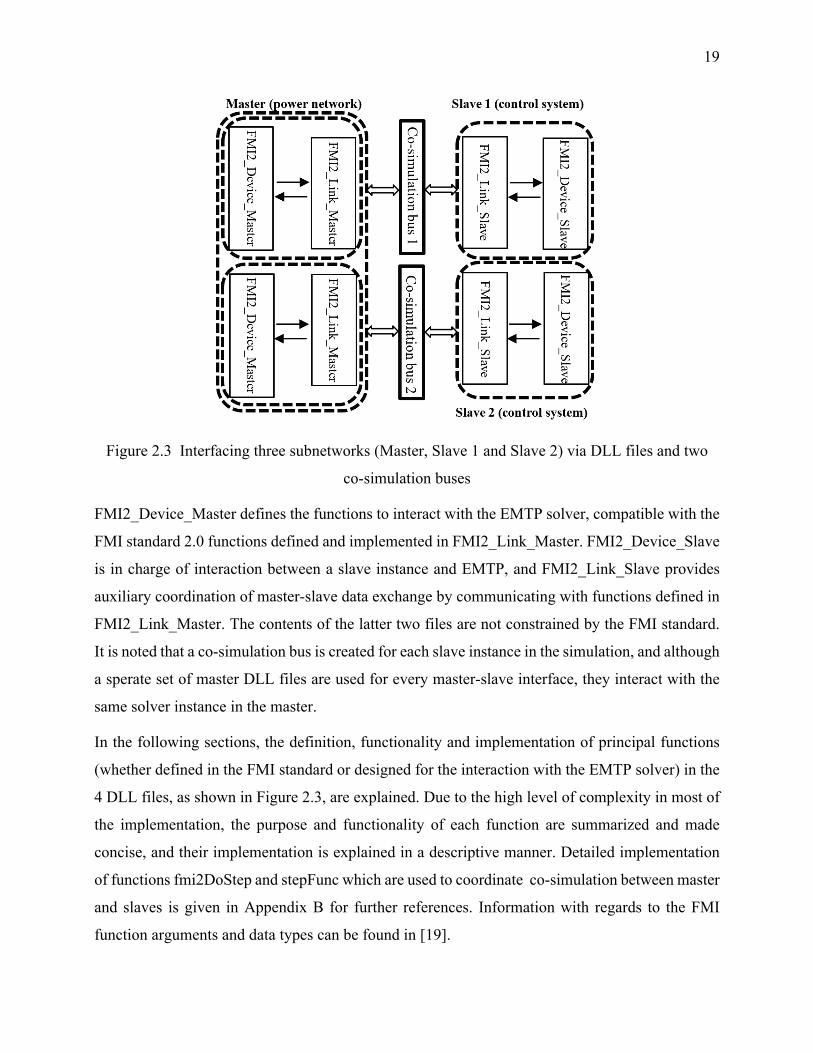
19

Figure 2.3 Interfacing three subnetworks (Master, Slave 1 and Slave 2) via DLL files and two

co-simulation buses

FMI2_Device_Master defines the functions to interact with the EMTP solver, compatible with the

FMI standard 2.0 functions defined and implemented in FMI2_Link_Master. FMI2_Device_Slave

is in charge of interaction between a slave instance and EMTP, and FMI2_Link_Slave provides

auxiliary coordination of master-slave data exchange by communicating with functions defined in

FMI2_Link_Master. The contents of the latter two files are not constrained by the FMI standard.

It is noted that a co-simulation bus is created for each slave instance in the simulation, and although

a sperate set of master DLL files are used for every master-slave interface, they interact with the

same solver instance in the master.

In the following sections, the definition, functionality and implementation of principal functions

(whether defined in the FMI standard or designed for the interaction with the EMTP solver) in the

4 DLL files, as shown in Figure 2.3, are explained. Due to the high level of complexity in most of

the implementation, the purpose and functionality of each function are summarized and made

concise, and their implementation is explained in a descriptive manner. Detailed implementation

of functions fmi2DoStep and stepFunc which are used to coordinate co-simulation between master

and slaves is given in Appendix B for further references. Information with regards to the FMI

function arguments and data types can be found in [19].

20

2.1.3.1 Implementation of functions in FMI2_Link_Master

• fmi2Instantiate

This function is called by the master program in order to load an FMU at the beginning of the co-

simulation stage. It is called once for every slave (FMU) instance and returns an element of type

“fmiComponent”. Its principal execution routines are:

1) Allocate memory for an FMU object

2) Assign certain values to the object

3) Create a file with a specified instance name in the same path where the FMU is extracted

4) Read values from the xml file and assign those values to the created FMU object

5) Read the location of the netlist file of the FMU

• fmi2FreeInstance

This function releases the slave instance, that is to say, it releases all the memory allocated for the

FMU.

• fmi2SetDebugLogging

This function allows the master to choose whether the FMU can send log messages to the master

as well as the level of details in these messages.

• fmi2SetupExperiment

This function asks the FMU to configure the co-simulation. It includes function calls to setINI and

setIN [19].

• fmi2EnterInitializationMode

This function asks the FMU to enter the initialization mode in which variables with attributes

“initial” = “exact” or “approx” can be defined. It is noted that the co-simulation bus used for data

exchange between master and slave is realized by file mapping. Its main execution routines are:

1) Create the co-simulation bus, which is a file mapping object with a certain size

2) Create a map view associated with the file mapping object

21

3) Initialize certain elements in the co-simulation bus

4) Initialize all three synchronization semaphores by setting them to 0

5) Release semaphore SemInitialization to the slave, informing the slave that the co-

simulation bus is successfully created and asking the slave to connect to it

• fmi2ExitInitializationMode

This function asks the FMU to exist the initialization mode. It executes the following routines:

1) Wait for the slave to release semaphore SemMaster to finish the initialization mode

2) Release SemMaster to itself so that the master can start its execution in the case of

asynchronous mode

Details on synchronization semaphores and different co-simulation modes will be explained

hereinafter.

• fmi2Terminate

This function notifies the FMU that the simulation is terminated by releasing the semaphore

SemSlave one last time.

• fmi2Reset

This function demands that the FMU return to its initial state.

• fmi2SetReal, fmi2SetInteger, fmi2SetBoolean, fmi2SetString, fmi2GetReal,

fmi2GetInteger, fmi2GetBoolean, fmi2GetString

These functions allow to transfer values from the master to the slave and vice versa. They are called

at every simulation time-step of the master and can also be used to initialize variables in the FMU.

• fmi2GetStatus, fmi2GetRealStatus, fmi2GetIntegerStatus, fmi2GetBooleanStatus,

fmi2GetStringStatus

These functions are called by the master to require the status of the co-simulation.

• fmi2DoStep

22

A call to this function starts the calculation of a new time-step in the FMU. It consists principally

of the following execution routines:

1) Write the current communication time-point and the master numerical integration time-

step onto the co-simulation bus

2) Read from the co-simulation bus the current slave time-point and its numerical

integration time-step

3) Verify the co-simulation mode (synchronous or asynchronous)

a) If the co-simulation mode is synchronous

i. If the slave lags behind the master

ii. Release semaphore SemSlave to the slave

iii. Wait for semaphore SemMaster from the slave

iv. Go back to i.

b) If the co-simulation mode is asynchronous

i. If the current communication time-point is 0

A. Release SemSlave to the slave

ii. If the current communication time-point is larger than 0

A. Wait for SemMaster from the slave

B. Release SemSlave to the slave

2.1.3.2 Implementation of functions in FMI2_Device_Master

Functions defined and implemented in this file are used for interaction between the FMI and EMTP

solver. They are not constrained by the FMI standard and are executed by the master program.

• init

This function performs all necessary procedures in the initialization stage of the simulation. Its

principal execution routines are:

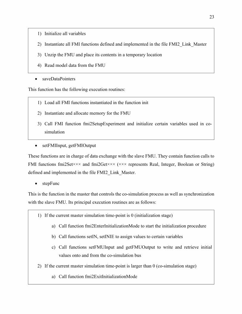
23

1) Initialize all variables

2) Instantiate all FMI functions defined and implemented in the file FMI2_Link_Master

3) Unzip the FMU and place its contents in a temporary location

4) Read model data from the FMU

• saveDataPointers

This function has the following execution routines:

1) Load all FMI functions instantiated in the function init

2) Instantiate and allocate memory for the FMU

3) Call FMI function fmi2SetupExperiment and initialize certain variables used in co-

simulation

• setFMIInput, getFMIOutput

These functions are in charge of data exchange with the slave FMU. They contain function calls to

FMI functions fmi2Set××× and fmi2Get××× (××× represents Real, Integer, Boolean or String)

defined and implemented in the file FMI2_Link_Master.

• stepFunc

This is the function in the master that controls the co-simulation process as well as synchronization

with the slave FMU. Its principal execution routines are as follows:

1) If the current master simulation time-point is 0 (initialization stage)

a) Call function fmi2EnterInitializationMode to start the initialization procedure

b) Call functions setIN, setINIE to assign values to certain variables

c) Call functions setFMUInput and getFMUOutput to write and retrieve initial

values onto and from the co-simulation bus

2) If the current master simulation time-point is larger than 0 (co-simulation stage)

a) Call function fmi2ExitInitializationMode

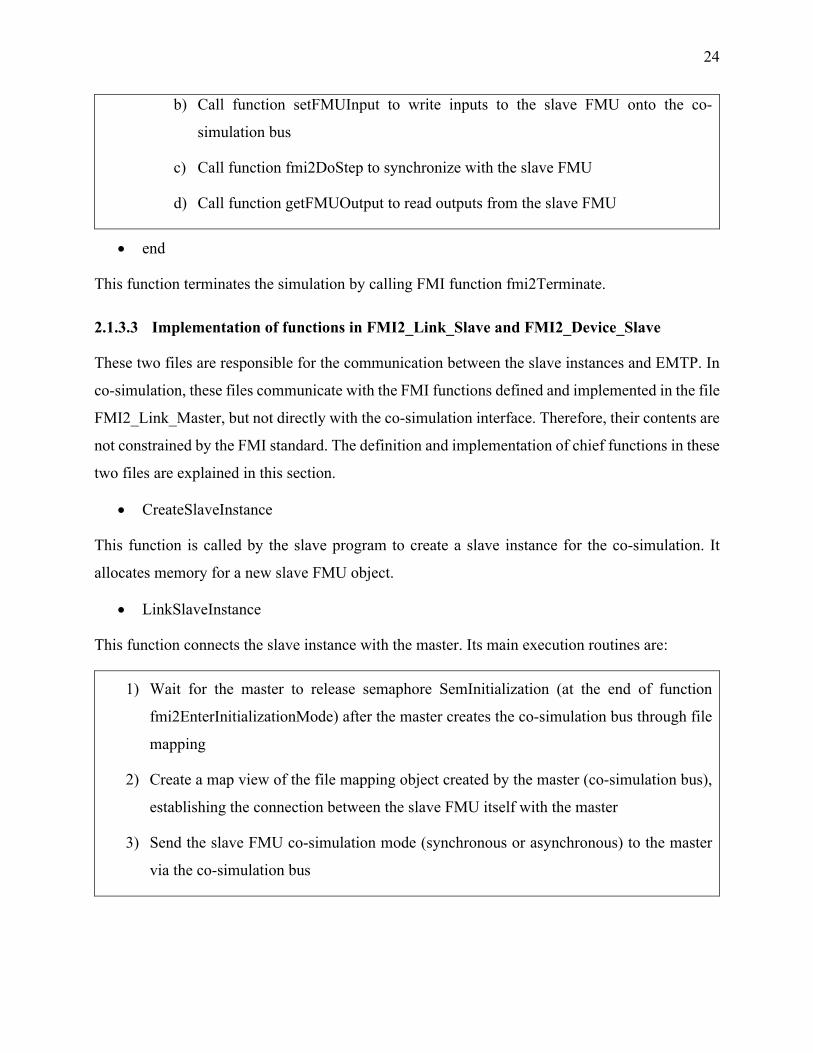
24

b) Call function setFMUInput to write inputs to the slave FMU onto the co-

simulation bus

c) Call function fmi2DoStep to synchronize with the slave FMU

d) Call function getFMUOutput to read outputs from the slave FMU

• end

This function terminates the simulation by calling FMI function fmi2Terminate.

2.1.3.3 Implementation of functions in FMI2_Link_Slave and FMI2_Device_Slave

These two files are responsible for the communication between the slave instances and EMTP. In

co-simulation, these files communicate with the FMI functions defined and implemented in the file

FMI2_Link_Master, but not directly with the co-simulation interface. Therefore, their contents are

not constrained by the FMI standard. The definition and implementation of chief functions in these

two files are explained in this section.

• CreateSlaveInstance

This function is called by the slave program to create a slave instance for the co-simulation. It

allocates memory for a new slave FMU object.

• LinkSlaveInstance

This function connects the slave instance with the master. Its main execution routines are:

1) Wait for the master to release semaphore SemInitialization (at the end of function

fmi2EnterInitializationMode) after the master creates the co-simulation bus through file

mapping

2) Create a map view of the file mapping object created by the master (co-simulation bus),

establishing the connection between the slave FMU itself with the master

3) Send the slave FMU co-simulation mode (synchronous or asynchronous) to the master

via the co-simulation bus

25

4) Release semaphore SemMaster to the master, informing the latter that the slave is now

“linked”

• LinkSlaveIsReadyForStep

This function waits for the master to modify its outputs to the FMU in order to retrieve the current

simulation time-point and numerical integration time-step of the master. It then updates the co-

simulation bus with the current simulation time-point and numerical integration time-step of the

slave. Its execution routines are:

1) Wait for the master to release semaphore SemSlave to the slave

2) Read master’s current simulation time-point and its numerical integration time-step from

the co-simulation bus

3) Write the slave’s current simulation time-point and its numerical integration time-step

onto the co-simulation bus

• LinkSlaveStepEnded

This function is called after the slave has advanced one step in time. It verifies if the slave lags

behind the master and can ask the slave to catch up with the master depending on the specific co-

simulation mode. At the end, it releases semaphore SemMaster to the master to authorize the latter

to advance in its calculation.

• LinkSlaveTerminate

This function is called at the end of the simulation to terminate the slave instance.

• LinkSlaveReadInput, LinkSlaveSetOutput

These functions allow the slave instance to retrieve its inputs from the co-simulation bus before

advancing one step in time or to write its output onto the co-simulation bus after the calculation of

one step.

2.1.4 Function calling sequence in the master and slave programs

The master program is responsible for the entire co-simulation process. It is in charge of the

communication with different FMUs and the general orchestration of the co-simulation. There

26

exists therefore an algorithm, namely the master algorithm, to fulfill the tasks of such a role. This

algorithm is implemented in the DLL file FMI2_Device_Master. The master algorithm is not

defined in the FMI standard. Hence, different implementations of such an algorithm are allowed.

One possible solution is illustrated in Figure 2.4. It is given in the form of UML 2.0 state machine.

More details about this solution can be found on Page 103 in [19].

The master algorithm controls the co-simulation process by calling the FMI functions defined and

implemented in the DLL file FMI2_Link_Master and coordinating them with the EMTP solver.

Considering the specifics of the implementation platform (the EMT-type solver in [2]), the master

algorithm adopted in this thesis (communication between the two DLL files FMI2_Device_Master

and FMI2_Link_Master) in terms of function calling sequence is presented in Figure 2.5. It is noted

that the dotted red arrows denote that functions in the file FMI2_Link_Master are called by those

in the file FMI2_Device_Master. Based on Figure 2.5, the master algorithm can be summarized as

follows:

1. Initialization

a. Unzip slave FMUs and instantiate master-slave interface instances

b. Load FMI functions from the DLL file and read model data from the xml file

c. Ask the slaves to configure the co-simulation

d. Create co-simulation bus

e. Initialize synchronization semaphores

2. Co-simulation

a. Exchange data and synchronize with slaves

b. Solve for the power network, advance one time-step then go back to step 2a

3. Terminate co-simulation

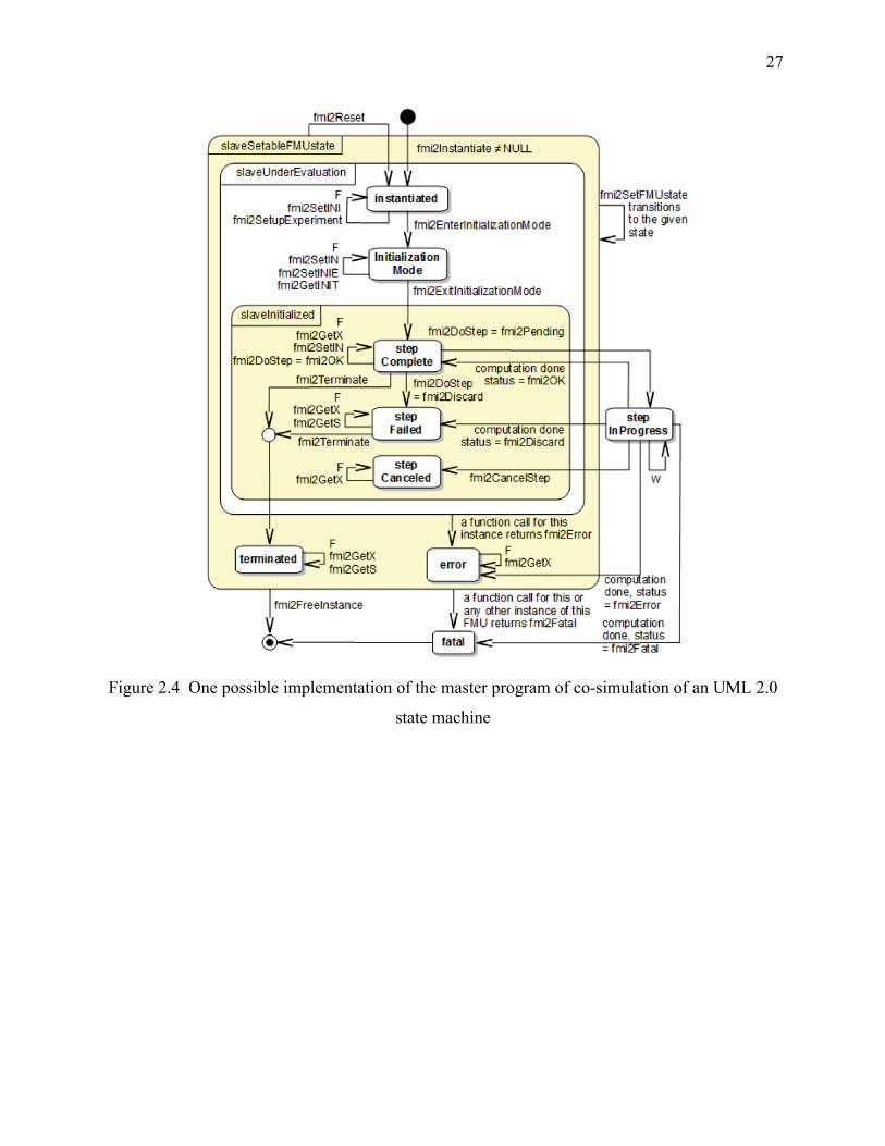
27

Figure 2.4 One possible implementation of the master program of co-simulation of an UML 2.0

state machine

28

Figure 2.5 Principal function calling sequence in the master algorithm

FMI2_Device_Master FMI2_Link_Master

fmi2Instantiate

fmi2SetDebugLogging

fmi2SetupExperiment

fmi2EnterInitializationMode

setFMUInput

getFMUOutput

fmi2ExitInitializationMode

setFMUInput

fmi2DoStep

getFMUOutput

fmi2Terminate

init

saveDataPointers

stepFunc

end

Initialization

Calculation

29

The slave algorithm answers to the master by performing tasks demanded by the master. The

principal function calling sequence in the slave algorithm adopted in this thesis, based on the

definition and implementation of slave functions explained in the previous section, is presented in

Figure 2.6. Once again, the dotted red arrows indicate that functions in the DLL file

FMI2_Link_Slave are called by those in the DLL file FMI2_Device_Slave. It is to mention that

the functions LinkSlaveSetOutput and LinkSlaveStepEnded inside the DLL file FMI2_Link_Slave

(as enclosed in the dotted green rectangle with rounded corners) are only called by the function

LoadObservables for the calculation of the first time-step.

Figure 2.6 Principal function calling sequence in the slave algorithm

FMI2_Link_Slave FMI2_Device_Slave

CreateSlaveInstance

LinkSlaveInstance

LinkSlaveIsReadyForStep

init

saveDataPointers

update

Calculation

LinkSlaveReadInput

LinkSlaveStepEnded

LinkSlaveSetOutput

LinkSlaveIsReadyForStep

LinkSlaveReadInput

LinkSlaveStepEnded

LinkSlaveSetOutput

LinkSlaveTerminate

LoadObservablesT0

LoadObservables

end

Initialization

30

As is observed in Figure 2.6, the slave algorithm can be described as follows:

1. Initialization

a. Create slave instances and load slave DLL functions

b. Connect slave instances to the co-simulation bus after the latter is created

c. Solve for the control system at 0t =

2. Co-simulation

a. Exchange data and synchronize with the master

b. Solve for the control system, advance to the next time-point, then go back to step

2a

3. Terminate slave instances

2.2 Co-simulation management

This section tackles the synchronization between master and slaves using low-level

synchronization primitive semaphore as well as master-slave data exchange with the help of file

mapping. Code details of important functions used in semaphore management are presented, and

two co-simulation modes (synchronous and asynchronous) are introduced. The structure and

implementation of the co-simulation bus used in master-slave data exchange are explained.

2.2.1 Synchronization between master and slaves

The synchronization between the master and slave subsystems is achieved through the

implementation of low-level synchronization primitive semaphores in the DLL files

FMI2_Link_Master and FMI2_Link_Slave. A semaphore, serving both as a lock and a condition

variable, is a variable used to control read and write access to a shared resource by multiple

processes or threads in a concurrent programming environment to prevent race conditions and other

concurrency problems [85] (see also [16]). By calling the pre-built function

WaitSemaphoreTimeOut on a specified semaphore, the current program (either master or slave)

temporarily halts its operation until the aforementioned semaphore is signaled, which indicates the

action of “waiting for a semaphore”; a call to the pre-built function ReleaseSemaphore on a

31

specified semaphore signals it and permits any program that is waiting for this semaphore to

continue with their operation, representing thus the action of “releasing a semaphore”.

2.2.1.1 Semaphore management

The implementation of the two pre-built functions WaitSemaphoreTimeOut and

ReleaseSemaphore are presented as follows:

• WaitSemaphoreTimeOut

bool WaitSemaphoreTimeOut(ModelInstance *comp, int SemNumber, int NumSemToWait, int TimeOut) { int ctr; HANDLE Sem1 = NULL; Sem1 = allocateSemaphore(comp->instanceName, SemNumber, comp->nbInputPins + comp->nbOutputPins); if (Sem1 != NULL) { for (ctr = 0; ctr < NumSemToWait; ctr++) { DWORD ret = WaitForSingleObject(Sem1, TimeOut); DWORD err = GetLastError(); if (ret != WAIT_OBJECT_0) { return false; } } return true; } return false;

}

• ReleaseSemaphore

bool ReleaseSemaphore(ModelInstance *comp, int SemNumber, int NumSemToRelease) { HANDLE Sem1; Sem1 = allocateSemaphore(comp->instanceName, SemNumber, comp->nbInputPins + comp->nbOutputPins); try { ReleaseSemaphore(Sem1, (LONG)NumSemToRelease, (LPLONG)NULL); } catch (Exception^ ex) { ex; return(false); } return true; }

32

where:

• comp: of type ModelInstance*, refers to a specific slave instance (FMU).

• SemNumber: of type integer, indicates the number of the semaphore, which is attached to

the name of the slave instance to uniquely identify the semaphore.

• NumSemWait: of type integer, is the number by which the semaphore count is decreased.

• NumSemToRelease: of type integer, is the number by which the semaphore count is

increased.

An auxiliary function named allocateSemaphore, whose functionality is self-evident, is also used

in the implementation of the aforementioned two pre-built functions:

• allocateSemaphore

HANDLE allocateSemaphore(fmi2String name_instance, int numSem, int nb_Pins_max) { HANDLE hdl = NULL; DWORD ret = 0; char name[256]; map<string, HANDLE>::iterator it; sprintf_s(name, "%sSem%d", name_instance, numSem); it = sem_hdl.find(name); if (it == sem_hdl.end()) { hdl = OpenSemaphoreA(SEMAPHORE_ALL_ACCESS, false, name); ret = GetLastError(); if (hdl == NULL) { hdl = CreateSemaphoreA(NULL, 0, nb_Pins_max + 1, name); ret = GetLastError(); } sem_hdl[name] = hdl; } else { hdl = (HANDLE)it->second; } return hdl;

}

where:

• nb_Pins_max: of type integer, defines the maximum count of the semaphore.

Another function used in semaphore management in the algorithm is named closeSemaphore,

whose implementation is as follows:

33

• closeSemaphore

bool closeSemaphore(fmi2String name_instance, int numSem) { HANDLE hdl; hdl = allocateSemaphore(name_instance, numSem, 1); if (hdl) { char name[256]; map<string, HANDLE>::iterator it; it = sem_hdl.find(name); if (it != sem_hdl.end()) { sem_hdl.erase(it); } CloseHandle(hdl); } return true;

}

A total of three semaphores are employed in the initialization and co-simulation stages in both the

master and slave algorithms, with the names SemInitialization, SemMaster and SemSlave. The first

one is used in the initialization mode, allowing a slave instance to connect to the co-simulation bus

created by the master. The second one is released by the slave to the master after the former finishes

certain operations. Similarly, the third one is released by the master to the slave, permitting the

latter to continue with its operations. For demonstrative purposes, only one slave instance is

considered in the following discussions.

2.2.1.2 Master-slave synchronization: initialization mode

After loading each FMU, the master starts the simulation and enters the initialization stage by

calling function fmi2EnterInitalizationMode, in which the master creates the co-simulation bus,

releases SemInitialization to the slave and writes initial conditions onto the co-simulation bus

whilst the slave waits for SemInitialization. Once the slave receives SemInitialization, it connects

to the co-simulation bus, writes its initial parameters onto it and releases SemMaster. As a result,

the master receives SemMaster from the slave and finishes the initialization stage. The

synchronization scheme between master and slave during the initialization stage is illustrated in

Figure 2.7. It is worth noting:

1) Every arrow represents an “exchange” of semaphore between the master and slave.

34

2) The start of the arrow represents the call to function ReleaseSemaphore, in which the

program involved “releases” the semaphore by increasing its count.

3) The end of the arrow represents the call to function WaitSemaphoreTimeOut, in which the

program involved “waits for” the semaphore by decreasing its count in order to further

continue its operations.

Figure 2.7 Synchronization scheme between master and slave during initialization stage

2.2.1.3 Master-slave synchronization: synchronous mode (with a single numerical

integration time-step)

As was stated earlier on in this thesis, two co-simulation modes are designed for the new off-line

simulation approach: the asynchronous and synchronous mode. The synchronous mode, despite its

sequential nature, allows not only using a single time-step in all master and slave subsystems, but

also different numerical integration time-steps in the master and each slave subsystem.

For the synchronous mode with a single numerical integration time-step in both master and slave,

as is shown in Figure 2.8, the master releases SemSlave to the slave such that the slave could read

inputs from the master, write output to the master, release SemMaster to the master, solve for the

current time-point and advance one time-step. Consequently, the master receives SemMaster from

the slave, retrieves the outputs from the slave and continues its own execution by advancing one

time-step as well. Hence, the execution of master and slave(s) is performed sequentially.

35

Figure 2.8 Synchronization scheme between master and slave in synchronous mode (with a

single numerical integration time-step)

2.2.1.4 Master-slave synchronization: asynchronous mode (with a single numerical

integration time-step)

In the asynchronous mode, the solutions of master and slave subsystems are executed in parallel

with a single numerical integration time-step on separate logical processors.

Specifically, in the asynchronous mode with a single numerical integration time-step in both master

and slave, the master first waits for the slave to release SemMaster after the solution of the previous

time-point. It then immediately releases SemSlave to the slave such that the slave can solve for its

current time-point and advance one time-step in time. Meanwhile, the master solves for the current

time-point likewise, advances one time-step and again waits for the release of SemMaster from the

slave, as is illustrated in Figure 2.9. Therefore, in the asynchronous mode, the master and the

slave(s) can each execute their computations simultaneously in parallel.

36

Figure 2.9 Synchronization scheme between master and slave in asynchronous mode (with a

single numerical integration time-step)

2.2.1.5 Master-slave synchronization: synchronous mode (with different numerical

integration time-steps)

In the synchronous mode with different numerical integration time-steps utilized in master and

slave subsystems, the principle of operation is similar to that of the synchronous mode with a single

numerical integration time-step. Nonetheless, a few changes have been made in the FMI function

fmi2DoStep, as is shown in Figure 2.10. Before releasing and waiting for any semaphores, the

fmi2DoStep function first compares the current time-point of the master and the slave. If the master

lags behind the slave, which occurs when the master’s numerical integration time-step is smaller

than that of the slave, function fmi2DoStep terminates without performing any tasks and the master

continues executing its calculation in time without releasing or waiting for any semaphores until

its current simulation time-point catches up with that of the slave. On the contrary, if the slave lags

behind the master with the numerical integration time-step of the slave smaller than that of the

master, the master keeps releasing SemSlave to the slave whilst staying in the loop in order that

the slave continues advancing in time and executing its calculation until it no longer lags behind

the master. The master thereby retrieves the outputs from the slave and continues its execution.

Once again, the execution of master and slave(s) is performed in sequence.

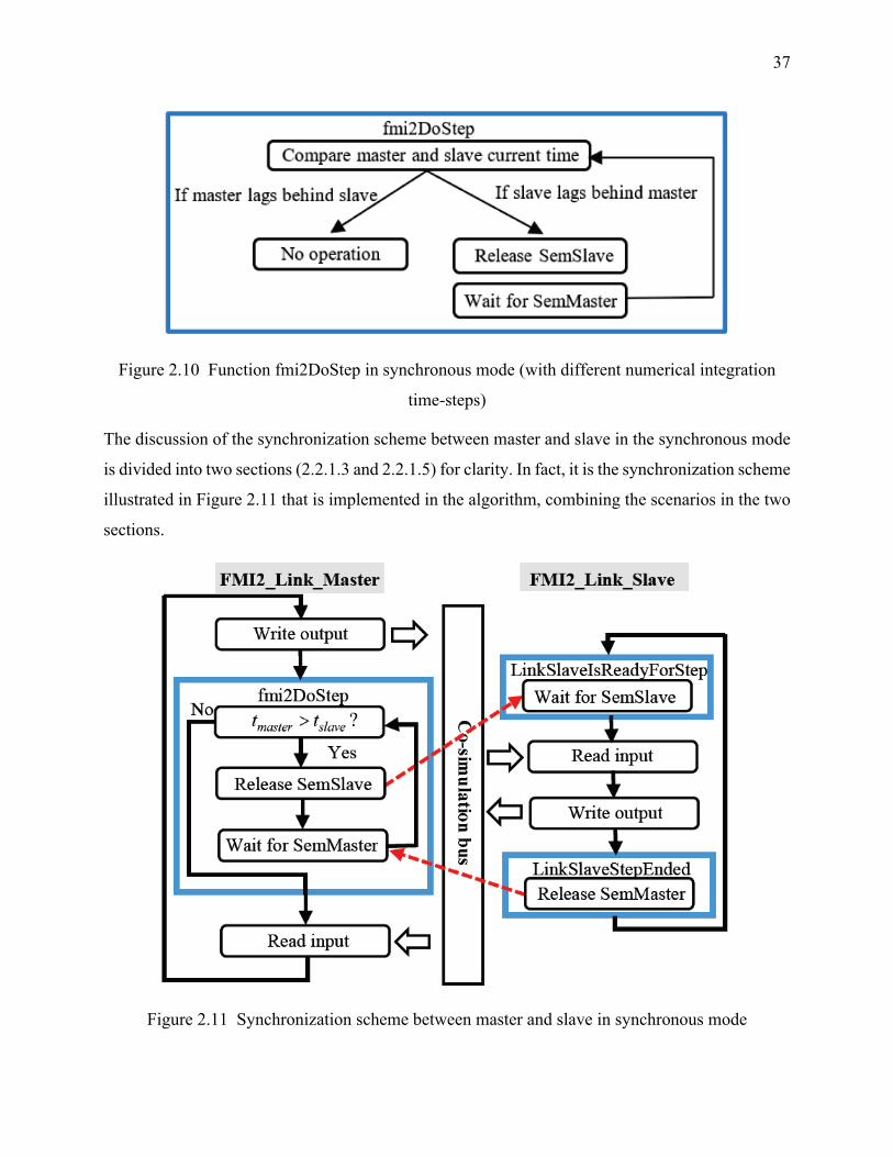
37

Figure 2.10 Function fmi2DoStep in synchronous mode (with different numerical integration

time-steps)

The discussion of the synchronization scheme between master and slave in the synchronous mode

is divided into two sections (2.2.1.3 and 2.2.1.5) for clarity. In fact, it is the synchronization scheme

illustrated in Figure 2.11 that is implemented in the algorithm, combining the scenarios in the two

sections.

Figure 2.11 Synchronization scheme between master and slave in synchronous mode

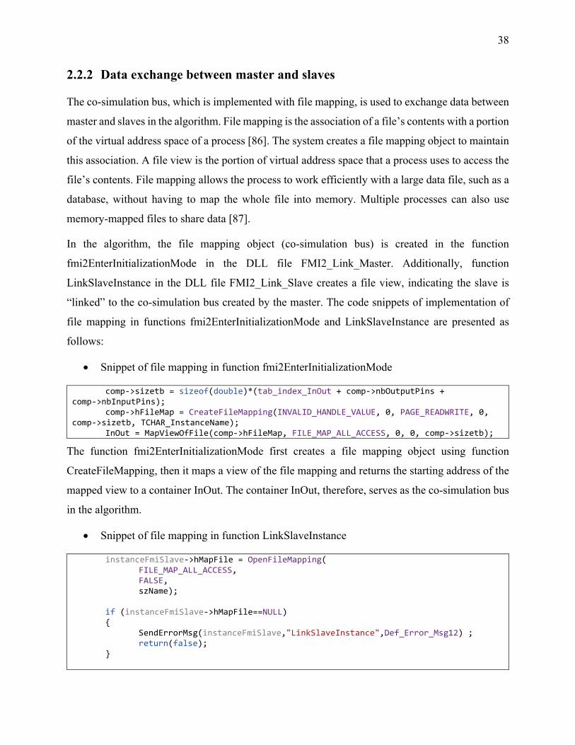
38

2.2.2 Data exchange between master and slaves

The co-simulation bus, which is implemented with file mapping, is used to exchange data between

master and slaves in the algorithm. File mapping is the association of a file’s contents with a portion

of the virtual address space of a process [86]. The system creates a file mapping object to maintain

this association. A file view is the portion of virtual address space that a process uses to access the

file’s contents. File mapping allows the process to work efficiently with a large data file, such as a

database, without having to map the whole file into memory. Multiple processes can also use

memory-mapped files to share data [87].

In the algorithm, the file mapping object (co-simulation bus) is created in the function

fmi2EnterInitializationMode in the DLL file FMI2_Link_Master. Additionally, function

LinkSlaveInstance in the DLL file FMI2_Link_Slave creates a file view, indicating the slave is

“linked” to the co-simulation bus created by the master. The code snippets of implementation of

file mapping in functions fmi2EnterInitializationMode and LinkSlaveInstance are presented as

follows:

• Snippet of file mapping in function fmi2EnterInitializationMode

comp->sizetb = sizeof(double)*(tab_index_InOut + comp->nbOutputPins + comp->nbInputPins); comp->hFileMap = CreateFileMapping(INVALID_HANDLE_VALUE, 0, PAGE_READWRITE, 0, comp->sizetb, TCHAR_InstanceName); InOut = MapViewOfFile(comp->hFileMap, FILE_MAP_ALL_ACCESS, 0, 0, comp->sizetb);

The function fmi2EnterInitializationMode first creates a file mapping object using function

CreateFileMapping, then it maps a view of the file mapping and returns the starting address of the

mapped view to a container InOut. The container InOut, therefore, serves as the co-simulation bus

in the algorithm.

• Snippet of file mapping in function LinkSlaveInstance

instanceFmiSlave->hMapFile = OpenFileMapping( FILE_MAP_ALL_ACCESS, FALSE, szName); if (instanceFmiSlave->hMapFile==NULL) { SendErrorMsg(instanceFmiSlave,"LinkSlaveInstance",Def_Error_Msg12) ; return(false); }

39

buffer1= (LPVOID) MapViewOfFile(instanceFmiSlave->hMapFile, FILE_MAP_ALL_ACCESS, 0, 0,

size1);

CopyMemory(bufferNbinOut1, buffer1,size1); instanceFmiSlave->nbOutputPins=int(bufferNbinOut1[tab_index_Nbout]); instanceFmiSlave->nbInputPins=int(bufferNbinOut1[tab_index_Nbin]); instanceFmiSlave->sizeBuf=sizeof(double)*(tab_index_InOut+instanceFmiSlave->nbOutputPins+instanceFmiSlave->nbInputPins); InOut = (LPVOID) MapViewOfFile(instanceFmiSlave->hMapFile, FILE_MAP_ALL_ACCESS, 0, 0,

instanceFmiSlave->sizeBuf);

Subsequently, the slave instance creates a mapped view using the handle returned by the file

mapping object created in the function fmi2EnterInitializationMode and “links” itself to the co-

simulation bus. The structure of the container InOut (co-simulation bus) is illustrated in Table 2.4.

Table 2.4 Structure of the container InOut (co-simulation bus)

Contents Index NbIn 0 NbOut 1 Slave Mode 2 Time Out 3 Time Slave 4 Step Slave 5 Time Master 6 Step Master 7 Error Master 8 Error Slave 9 Y_1 10 … … Y_NbIn 9+NbIn X_1 10+NbIn … … X_NbOut 9+NbIn+NbOut

where:

• NbIn: the number of inputs of the slave instance.

• NbOut: the number of outputs of the slave instance.

40

• Slave Mode: the chosen co-simulation mode of the slave instance.

• Time Out: the chosen maximum synchronization time.

• Time Slave: the slave simulation time-point.

• Step Slave: the slave numerical integration time-step.

• Time Master: the master simulation time-point.

• Step Master: the master numerical integration time-step.

• Error master: the value is 1 if the master signals an error; 0 if not.

• Error slave: the value is X if the Xth input or output of the slave cannot be updated; 0 if not.

• Y and X: different inputs and outputs of the slave instance.

The total size of the container InOut is thus NbIn+NbOut+10.

2.3 Improvements on the original methodology

In the previous section, two co-simulation modes, the parallel asynchronous mode and the

sequential synchronous mode, were proposed, in which only the latter could accommodate the use

of different numerical integration time-steps in different decoupled subsystems. Based on the this

methodology and continuing with the master-slave co-simulation scheme adopted in this thesis, in

this section, the computation capacity of the parallel asynchronous mode is extended into

accommodating the use of different numerical integration time-steps in different subsystems

decoupled in memory, greatly improving simulation flexibility and efficiency. Furthermore, a

signal correction procedure based on linear extrapolation is introduced to achieve higher accuracy

in a multistep simulation environment.

2.3.1 Parallel multistep asynchronous mode

The improved asynchronous mode is divided into 3 scenarios based on the comparison of master

and slave numerical integration time-steps. The synchronization scheme between master and slave

in the improved parallel multistep asynchronous mode is presented in Figure 2.12. It is noted that

the 3 scenarios are indicated by the 3 blue boxes, and only one scenario is executed in practice.

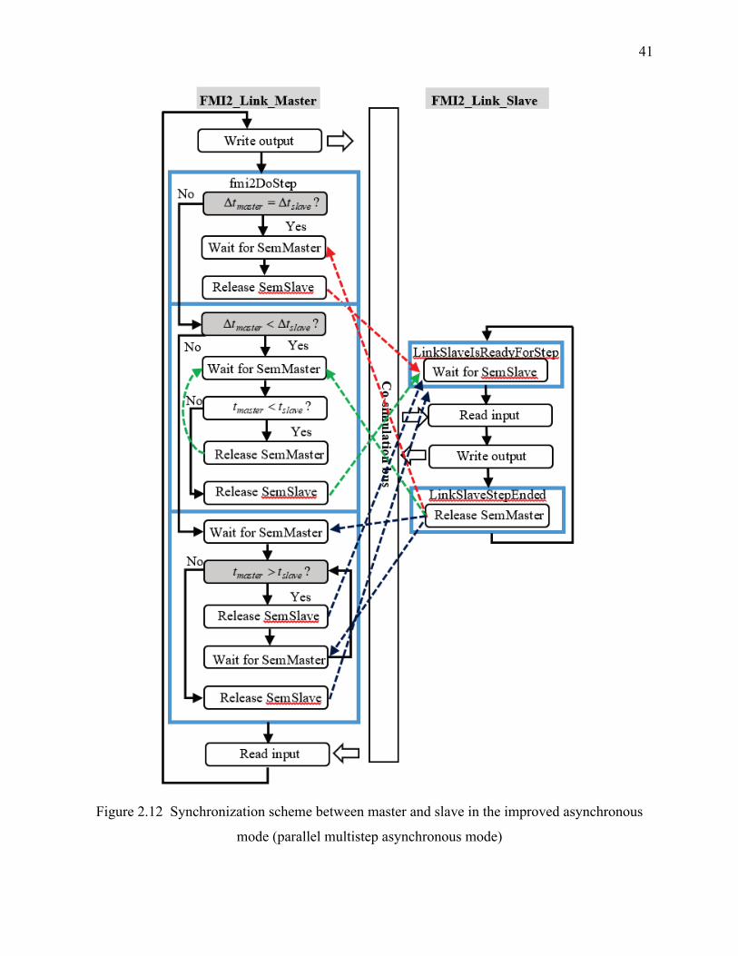
41

Figure 2.12 Synchronization scheme between master and slave in the improved asynchronous

mode (parallel multistep asynchronous mode)

42

The improved master-slave synchronization scheme for the parallel multistep asynchronous

illustrated in Figure 2.12 might seem daunting due to the level of complexity. A scenario-wise

explanation is hence needed to understand its principle of operation. The 3 different scenarios are

separated based on the comparison of master and slave numerical integration time-steps and are

presented respectively in Figure 2.13, Figure 2.14 and Figure 2.15. It is worthwhile to note that all

arrows, in spite of their colors, denote the release of semaphore.

Figure 2.13 First synchronization scenario ( master slavet t∆ = ∆ ) between master and slave in the

parallel multistep asynchronous mode

43

Figure 2.14 Second synchronization scenario ( master slavet t∆ < ∆ ) between master and slave in the


44

Figure 2.15 Third synchronization scenario ( master slavet t∆ > ∆ ) between master and slave in the


The first scenario (Figure 2.13) in which master slavet t∆ = ∆ is the case implemented in the original

methodology discussed in the previous section. Figure 2.13 and Figure 2.9, therefore, describe the

same principle of operation.

In the second scenario where master slavet t∆ < ∆ , as is shown in Figure 2.14, after waiting for the

slave to release SemMaster, the master compares its current simulation time-point with that of the

slave. If the master lags behind the slave due to having a smaller numerical integration time-step,

it releases SemMaster to itself, solves for its current time-point and advances one step in time. It

keeps releasing SemMaster to itself so that it can advance without the help from the slave till its

current simulation time-point catches up with that of the slave. Once the master catches up with

the slave, it releases SemSlave to the slave such that both can execute their subsequent calculation

simultaneously.

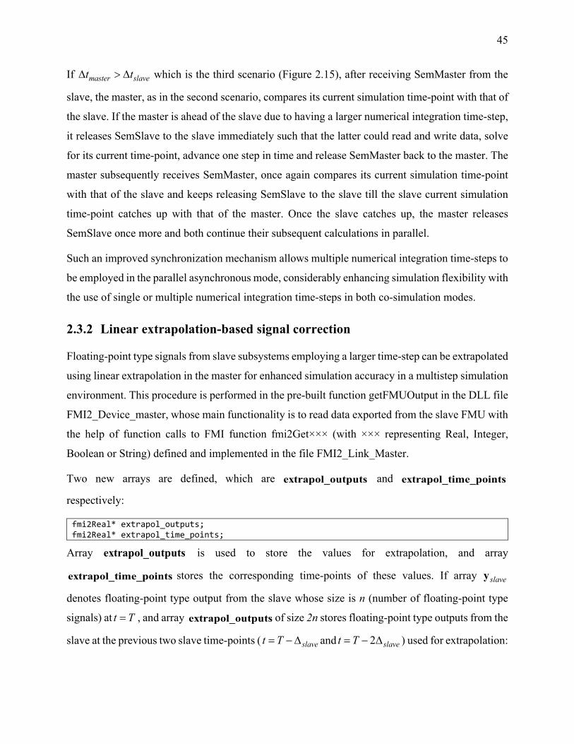
45

If master slavet t∆ > ∆ which is the third scenario (Figure 2.15), after receiving SemMaster from the

slave, the master, as in the second scenario, compares its current simulation time-point with that of

the slave. If the master is ahead of the slave due to having a larger numerical integration time-step,

it releases SemSlave to the slave immediately such that the latter could read and write data, solve

for its current time-point, advance one step in time and release SemMaster back to the master. The

master subsequently receives SemMaster, once again compares its current simulation time-point

with that of the slave and keeps releasing SemSlave to the slave till the slave current simulation

time-point catches up with that of the master. Once the slave catches up, the master releases

SemSlave once more and both continue their subsequent calculations in parallel.

Such an improved synchronization mechanism allows multiple numerical integration time-steps to

be employed in the parallel asynchronous mode, considerably enhancing simulation flexibility with

the use of single or multiple numerical integration time-steps in both co-simulation modes.

2.3.2 Linear extrapolation-based signal correction

Floating-point type signals from slave subsystems employing a larger time-step can be extrapolated

using linear extrapolation in the master for enhanced simulation accuracy in a multistep simulation

environment. This procedure is performed in the pre-built function getFMUOutput in the DLL file

FMI2_Device_master, whose main functionality is to read data exported from the slave FMU with

the help of function calls to FMI function fmi2Get××× (with ××× representing Real, Integer,

Boolean or String) defined and implemented in the file FMI2_Link_Master.

Two new arrays are defined, which are extrapol_outputs and extrapol_time_points

respectively:

fmi2Real* extrapol_outputs; fmi2Real* extrapol_time_points;

Array extrapol_outputs is used to store the values for extrapolation, and array

extrapol_time_points stores the corresponding time-points of these values. If array slavey

denotes floating-point type output from the slave whose size is n (number of floating-point type

signals) at t T= , and array extrapol_outputs of size 2n stores floating-point type outputs from the

slave at the previous two slave time-points ( slavet T= −∆ and 2 slavet T= − ∆ ) used for extrapolation:

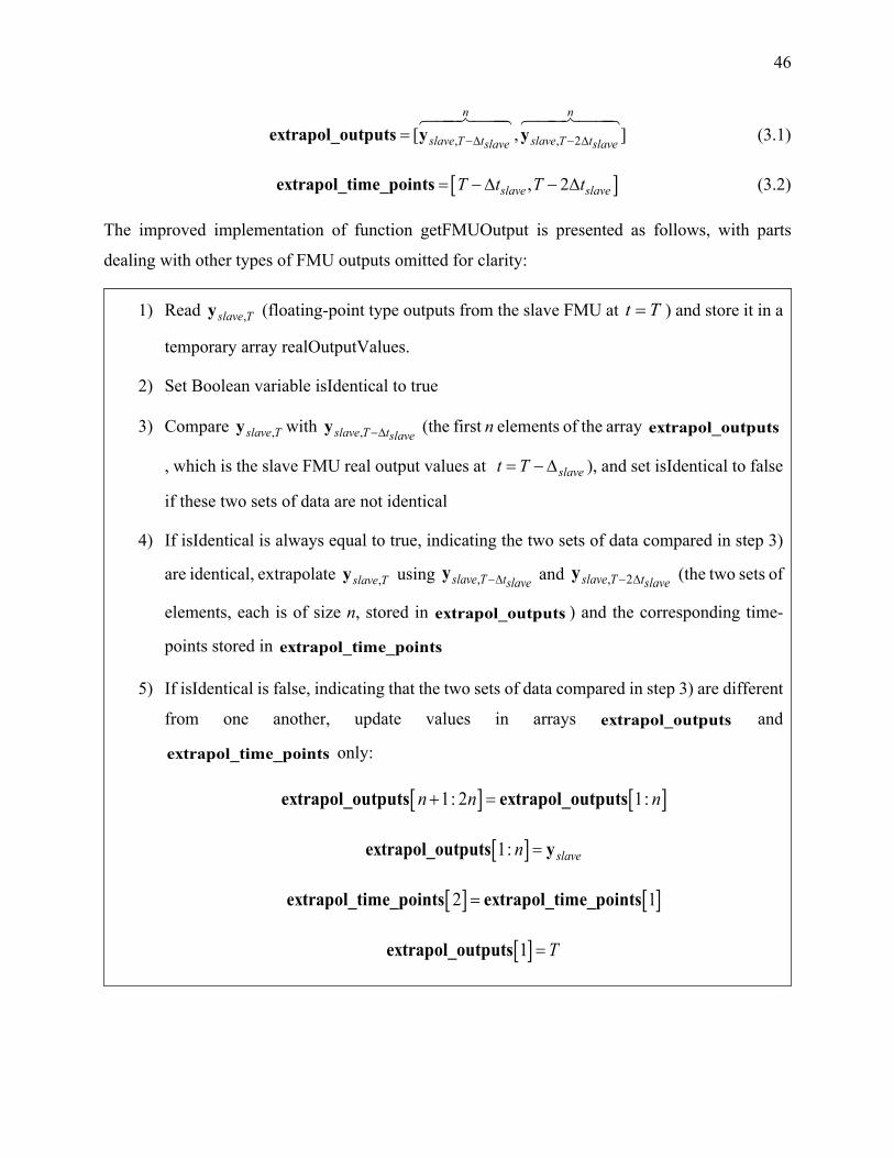
46

, , 2[ , ]n n

slave T t slave T tslave slave−∆ − ∆=extrapol_outputs y y

(3.1)

[ ], 2slave slaveT t T t= −∆ − ∆extrapol_time_points (3.2)

The improved implementation of function getFMUOutput is presented as follows, with parts

dealing with other types of FMU outputs omitted for clarity:

1) Read ,slave Ty (floating-point type outputs from the slave FMU at t T= ) and store it in a

temporary array realOutputValues.

2) Set Boolean variable isIdentical to true

3) Compare ,slave Ty with ,slave T tslave−∆y (the first n elements of the array extrapol_outputs

, which is the slave FMU real output values at slavet T= −∆ ), and set isIdentical to false

if these two sets of data are not identical

4) If isIdentical is always equal to true, indicating the two sets of data compared in step 3)

are identical, extrapolate ,slave Ty using ,slave T tslave−∆y and , 2slave T tslave− ∆y (the two sets of

elements, each is of size n, stored in extrapol_outputs ) and the corresponding time-

points stored in extrapol_time_points

5) If isIdentical is false, indicating that the two sets of data compared in step 3) are different

from one another, update values in arrays extrapol_outputs and

extrapol_time_points only:

[ ] [ ]1: 2 1:n n n+ =extrapol_outputs extrapol_outputs

[ ]1: slaven =extrapol_outputs y

[ ] [ ]2 1=extrapol_time_points extrapol_time_points

[ ]1 T=extrapol_outputs

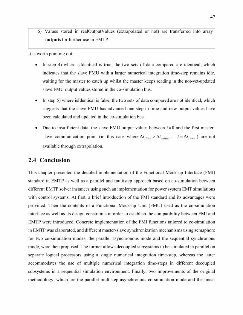
47

6) Values stored in realOutputValues (extrapolated or not) are transferred into array

outputs for further use in EMTP

It is worth pointing out:

• In step 4) where isIdentical is true, the two sets of data compared are identical, which

indicates that the slave FMU with a larger numerical integration time-step remains idle,

waiting for the master to catch up whilst the master keeps reading in the not-yet-updated

slave FMU output values stored in the co-simulation bus.

• In step 5) where isIdentical is false, the two sets of data compared are not identical, which

suggests that the slave FMU has advanced one step in time and new output values have

been calculated and updated in the co-simulation bus.

• Due to insufficient data, the slave FMU output values between 0t = and the first master-

slave communication point (in this case where slave mastert t∆ > ∆ , slavet t= ∆ ) are not

available through extrapolation.

2.4 Conclusion

This chapter presented the detailed implementation of the Functional Mock-up Interface (FMI)

standard in EMTP as well as a parallel and multistep approach based on co-simulation between

different EMTP solver instances using such an implementation for power system EMT simulations

with control systems. At first, a brief introduction of the FMI standard and its advantages were

provided. Then the contents of a Functional Mock-up Unit (FMU) used as the co-simulation

interface as well as its design constraints in order to establish the compatibility between FMI and

EMTP were introduced. Concrete implementation of the FMI functions tailored to co-simulation

in EMTP was elaborated, and different master-slave synchronization mechanisms using semaphore

for two co-simulation modes, the parallel asynchronous mode and the sequential synchronous

mode, were then proposed. The former allows decoupled subsystems to be simulated in parallel on

separate logical processors using a single numerical integration time-step, whereas the latter

accommodates the use of multiple numerical integration time-steps in different decoupled

subsystems in a sequential simulation environment. Finally, two improvements of the original

methodology, which are the parallel multistep asynchronous co-simulation mode and the linear

48

extrapolation-based signal correction procedure on floating-point slave outputs, were presented

with the goal of enhancing simulation flexibility, efficiency and accuracy.

49

CHAPTER 3 TEST CASES AND SIMULATION RESULTS OF THE

FMI-BASED APPROACH

This chapter presents simulation results of the FMI-based parallel and multistep approach

developed in this thesis. It first validates the design of the co-simulation interface in EMTP using

the FMI standard through a simple example, then proceeds to validate both the original and the

improved methodologies. The validation focuses on two aspects: accuracy and computation time

gains. Each aspect is validated using realistic power system simulation benchmarks with complex

control systems (wind generator controls and protection relays). Advantages of the proposed FMI-

based approach in terms of accuracy, efficiency and scalability are fully demonstrated.

3.1 Validation of the co-simulation interface design

In this section, the design of the co-simulation interface using the FMI standard on the EMT-type

solver [2] is validated through the demonstration of a simple example. Simulation results obtained

from both co-simulation modes are compared with those using EMTP without co-simulation. The

validation of the co-simulation interface design confirms that the implementation of the FMI

standard on the EMT-type solver [2] is successful, and further tests using realistic power system

simulation benchmarks can thereby be conducted.

3.1.1 Creation of master and slave models

The complete test circuit using the EMT-type solver [2] for the validation of the co-simulation

interface design is shown in Figure 3.1. This test circuit consists of two “real” type inputs which

are trigonometric functions sine and cosine and two “real” type outputs which are the sum of the

two inputs squared and the product of these two inputs respectively. As was mentioned previously,

the FMI standard is implemented in EMTP for control signals (integer, floating-point or Boolean)

that can be exchanged by means of the co-simulation interface in this thesis. Therefore, all the

circuit elements are represented using control blocks. In the original EMTP simulation without

using the FMI-based approach, the simulation interval is 100 ms with a numerical integration time-

step of 100 µs.

50

Figure 3.1 Test circuit for the validation of co-simulation interface design

In the FMI-based co-simulation approach, the section inside the red dotted rectangle with rounded

corners, as is shown in Figure 3.1, is taken out as the slave subsystem while the rest of the test

circuit being the master. Therefore, the slave subsystem using the FMI-based co-simulation

approach is given in Figure 3.2.

Figure 3.2 Slave subsystem for the validation of co-simulation interface design

The box named “Test_Slave FMI 2.0 (Slave)” indicates the circuit in the current design file is the

slave subsystem, and this box serves as the interface with the master. It has 2 inputs (Sin and Cos)

and 2 outputs (Output1, Output2). The directions of arrows at the box suggest that the inputs Sin

and Cos are the inputs “from” the master, and the outputs Output1 and Output2 are the outputs of

the slave “to” the master. The inputs and outputs, co-simulation mode, as well as other parameter

settings in order to generate the slave FMU file from the design file shown in Figure 3.2 are

presented in Figure 3.3 and Figure 3.4. The slave FMU can thus be generated after effectuating

these parameter settings accordingly.

f(u)

Sin

f(u)

Cos

PROD12

PROD12

PROD12

SUM12

scope Output1

scope Output2

PROD12

PROD12

PROD12

SUM12

Test_Slave

FMI 2.0(Slave)

CosSin

Output2Output1

Slave

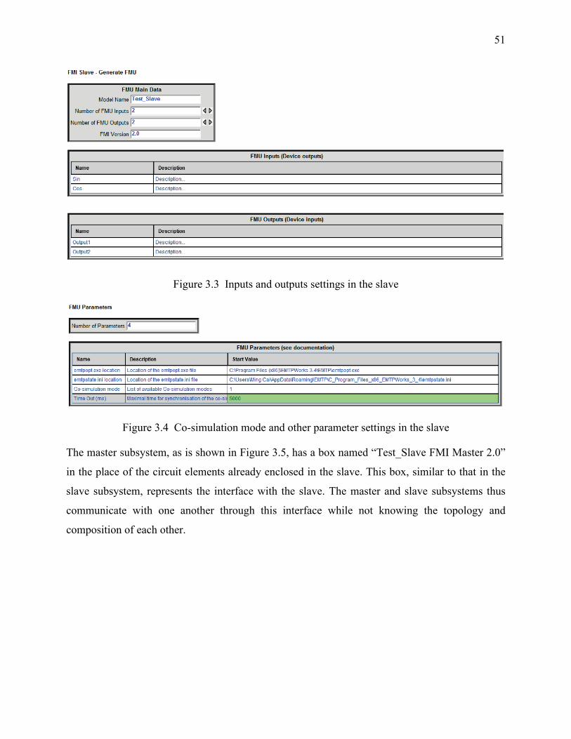
51

Figure 3.3 Inputs and outputs settings in the slave

Figure 3.4 Co-simulation mode and other parameter settings in the slave

The master subsystem, as is shown in Figure 3.5, has a box named “Test_Slave FMI Master 2.0”

in the place of the circuit elements already enclosed in the slave. This box, similar to that in the

slave subsystem, represents the interface with the slave. The master and slave subsystems thus

communicate with one another through this interface while not knowing the topology and

composition of each other.

52

Figure 3.5 Master subsystem for the validation of co-simulation interface design

After loading the generated slave FMU file into the interface represented by the box in Figure 3.5,

the master obtains all necessary data and information from the slave in order to execute co-

simulation. All loaded data and parameters of the slave in the master are presented in Figure 3.6.

(a) FMU main data

(b) FMU inputs

f(u)

Sin

f(u)

Cos

Test_Slave

FMI Master 2.0

CosSin

Output2Output1 scope Output1

scope Output2

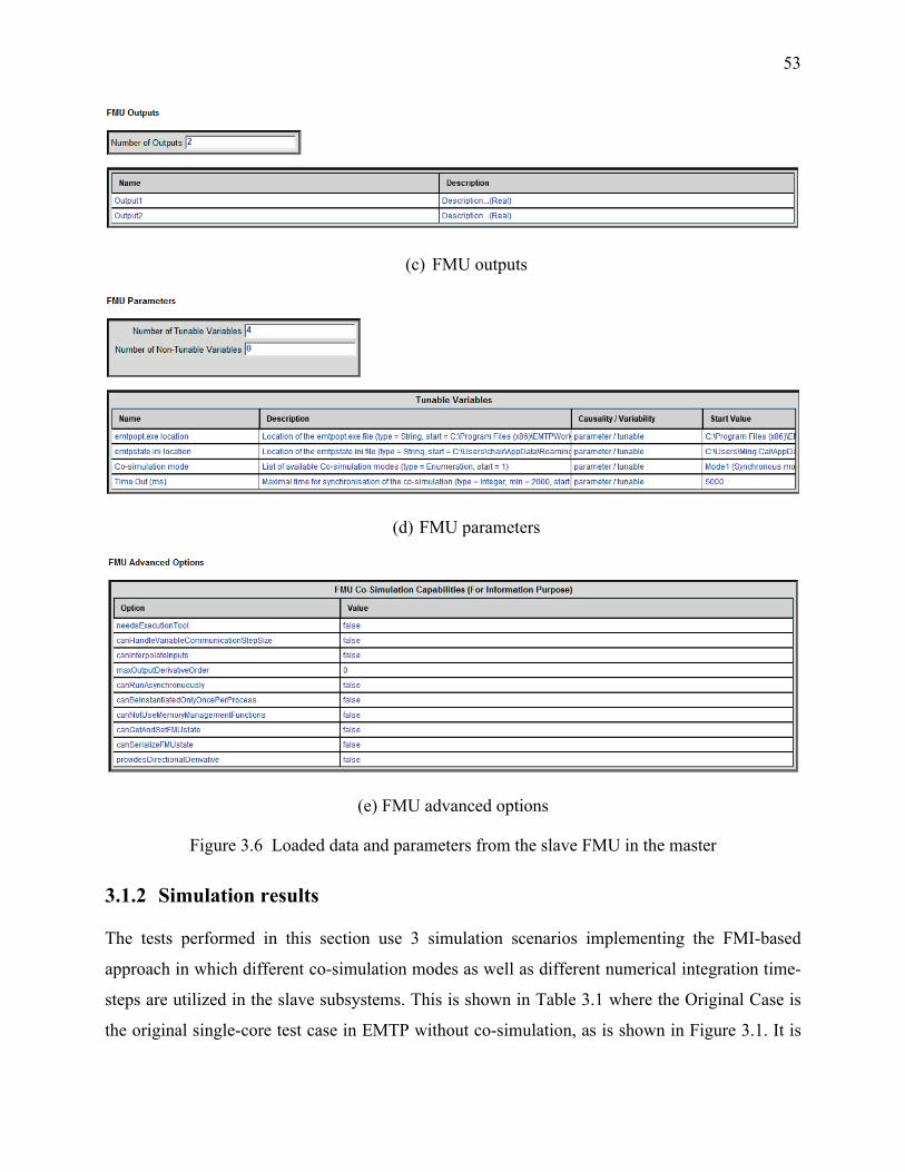
53

(c) FMU outputs

(d) FMU parameters

(e) FMU advanced options

Figure 3.6 Loaded data and parameters from the slave FMU in the master

3.1.2 Simulation results

The tests performed in this section use 3 simulation scenarios implementing the FMI-based

approach in which different co-simulation modes as well as different numerical integration time-

steps are utilized in the slave subsystems. This is shown in Table 3.1 where the Original Case is

the original single-core test case in EMTP without co-simulation, as is shown in Figure 3.1. It is

54

noted that although the master and slave concepts do not apply to the Original Case, the numerical

integration time-step of 100 µs used in the master and slave in this case indicates that 100 µs is the

numerical integration time-step of the entire test case. The simulation interval is 100 ms for all

cases. The waveforms of Output 1, Output 2 and closer observation of Output 2 within a short

interval in all simulation scenarios are presented in Figure 3.7, Figure 3.8 and Figure 3.9

respectively. For clear observation, only partial waveforms of the entire simulation interval are

shown.

Table 3.1 Co-simulation mode scenarios, co-simulation interface design validation

Co-simulation mode Master t∆ (µs) Slave t∆ (µs) Original Case N/A 100 100 Scenario 1 Synchronous 100 100 Scenario 2 Synchronous 100 200 Scenario 3 Asynchronous 100 100

Figure 3.7 Waveforms of Output 1 for all simulation scenarios

55

Figure 3.8 Waveforms of Output 2 for all simulation scenarios

Figure 3.9 Closer observation of waveform of Output 2 for all simulation scenarios

It is observed in Figure 3.7 and Figure 3.8 that the waveforms of Output 1 and Output 2 in all

simulation scenarios using the FMI-based co-simulation approach match well to those in the

Original Case without co-simulation. Nonetheless, upon closer observation of the waveform of

Output 2 within a short interval in all simulation scenarios, as presented in Figure 3.9, a delay of

one or two time-steps exists between the slave and the master in all scenarios using the FMI-based

co-simulation approach compared to the Original Case. It is worth noting that a one time-step delay

is manually added in the function stepFunc in the DLL file FMI2_Device_Master during the master

and slave data exchange for simulation stability and robustness. Therefore, the slave subsystem in

Scenario 1 (synchronous mode with a single time-step) exhibits a constant one time-step delay of

100 ms compared to the Original Case. The delays observed in the other scenarios are discussed in

detail in Section 3.2.1.3.

56

By and large, the simple test performed in this section has demonstrated that the co-simulation

interface in EMTP using the FMI standard developed in this thesis is functional. Further validation

on different aspects of the implementation can thus be conducted.

3.2 Validation of the original methodology

In this section, tests validating the original methodology, which is the two co-simulation modes

with master-slave synchronization schemes proposed in Section 2.2, are performed on practical

power system simulation benchmarks with complex control systems (wind generator control and

protection relays). The tests are performed focusing on two aspects: accuracy and computation

efficiency. Detailed error analysis and discussions on the observed computation time gains are also

provided.

3.2.1 Accuracy validation

Accuracy of the original methodology is verified by comparing various variables in a simulation,

such as offshore wind park outputs as well as line relay tripping instants after a perturbation (fault).

The reference waveforms are those found from the simulation using original EMTP single-core

benchmarks without co-simulation. In all cases, a multiphase unbalanced load-flow solution is

performed for initializing the time-domain solution where a fault condition is simulated.

3.2.1.1 Test case Network-1

The tests performed on Network-1 are to validate the accuracy of co-simulation in offshore wind

park control systems by observing the outputs of offshore wind parks through HVDC transmission.

4 simulation scenarios implementing the FMI-based co-simulation approach are used, in which

different co-simulation modes as well as different numerical integration time-steps are utilized in

the offshore wind generator control systems. This is shown in Table 3.2 where the Original Case

is the original single-core benchmark simulated on EMTP without co-simulation.

57


Network-1

Co-simulation mode Main network t∆ (µs)

WP control t∆(µs)

Original Case N/A 50 50 Scenario 1 Asynchronous 50 50 Scenario 2 Synchronous 50 50 Scenario 3 Synchronous 50 100 Scenario 4 Synchronous 50 200

The Network-1 benchmark is shown in Figure 3.10. It is the EMT version of the original IEEE-39

benchmark with onshore and offshore wind generation as well as HVDC transmission [88]. This

benchmark represents a portion of the 345-kV New England transmission grid [89], [90] consisting

of 4 voltage levels, 39 buses, 8 synchronous generators (the other 2 at buses B25 and B2 are

replaced by onshore and offshore wind parks), 34 transmission lines, 12 transformers, and 19 loads.

It modifies the original data [89], [90] by representing transmission lines using the CP model and

incorporating both static and dynamic load types, together with supplementary data in tower

geometry, conductor types, transformers, and machine controls. Further device modelling details

can be found in [1], [88] and [91]. This benchmark has a total of 1381 network nodes, with the

size of the main network equations (modified-augmented-nodal-analysis [2]) being 4826×4826

with 35718 non-zeros.

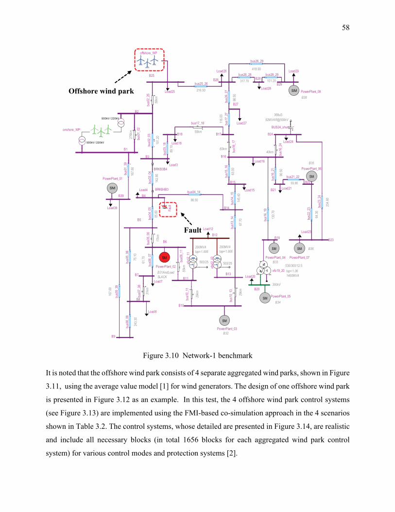
58

Figure 3.10 Network-1 benchmark

It is noted that the offshore wind park consists of 4 separate aggregated wind parks, shown in Figure

3.11, using the average value model [1] for wind generators. The design of one offshore wind park

is presented in Figure 3.12 as an example. In this test, the 4 offshore wind park control systems

(see Figure 3.13) are implemented using the FMI-based co-simulation approach in the 4 scenarios

shown in Table 3.2. The control systems, whose detailed are presented in Figure 3.14, are realistic

and include all necessary blocks (in total 1656 blocks for each aggregated wind park control

system) for various control modes and protection systems [2].

SM PowerPlant_09B38

SM

PowerPlant_06B35

SM

PowerPlant_01

SM

B31AndLoadSLACK

PowerPlant_02

SM

PowerPlant_03B32

SM PowerPlant_05B34

SM

PowerPlant_04B33

SM

PowerPlant_07

B36

+

317.70

bus26_28+

101.20bus28_29

+

418.90

bus26_29

Load29Load26

+

216.50

bus25_26Load28

Load25

PI

+

bus0

2_25

58km

CP

+bus0

2_03

101.2

0

+bu

s03_

18

89.10

Load18

Load3

PI+

bus0

1_02

276k

m+

bus0

1_39

167.6

0

+bus0

3_04

142.8

0

Load4

Load39 +bu

s04_

05

85.80

PI

+

bus0

5_06

17km

+bus0

6_07

61.70

Load7

PI

+31

km

bus0

7_08

+bu

s05_

08

75.10

+bu

s09_

39

167.6

0

+bu

s08_

09

243.3

0

Load8

+bus2

6_27

98.50

+bus1

7_27

116.0

0

PI

+

bus17_18

55km

PI+

bus1

6_17

60km PI+

bus1

6_24

40km

+bu

s15_

16

63.00 +

bus1

6_21

90.50

+bu

s14_

15

145.4

0

+bu

s16_

19

130.7

0

+bus2

2_23

64.30

+bus2

3_24

234.6

0

+bus21_22

93.80

+bus04_14

86.50

PI+ bu

s06_

1155

km

2 3

1

xfo19_20530/300/12.5tap=1.061400MVA

+bu

s13_

14

67.70

PI

+29

km

bus1

0_13

PI+

29km

bus1

0_11

Load27

Load24

Load16

Load12

Load20

Load23

Load15

+

BUS24_shunt

368uS92MVAR@500kV

Load21

F

Fault

BRKB3B4

BRKB4B3

12 -30

503/25

xfo12

_13

200MVAtap=1.006

12 -30

503/25xfo12

_11

200MVAtap=1.006

offshore_WP

500kV / 220kV

500kV / 220kV

onshore_WP

B29B28

B25

B7

B39

B9

B8

B27

B26

B17B18

B23

B24

B22

B21

B6

B11

B19

B13

B10

300kVB20

B16B3

B14

B5

B15

B12

B4

B1

B2

Offshore wind park

Fault

59

Figure 3.11 Offshore wind parks and HVDC connection in Network-1

Figure 3.12 Design of one offshore wind park in Network-1

PI+ PI1

2

3

1

150/34.5/34.5

TR1

2

3

1

150/34.5/34.5

TR2

PI+ PI2

2.32

518

.605

625O

hm

ZZ_1

3

2.32

518

.605

625O

hm

ZZ_1

2

2.32

518

.605

625O

hm

ZZ_2

2

2.32

518

.605

625O

hm

ZZ_2

3

EquivalentPI Circuit Parameters




PQ_VSC_offshoregrid

PQ_VSC_onshoreP1 P2

N2N1

Cable_70kmMMC

monopolemodel4400 SM

VSC_onshore

R

chopper

MMC

monopolemodel4400 SM

VSC_offshore

DFIG AVMWP_AVM1

Ppark_MW= 150;Vgrid_kV= 34.5;ControlMode= 1

DFIG AVMWP_AVM2


DFIG AVMWP_AVM3


DFIG AVM

WP_AVM4


grid

PCC

+

10MR1

meas1 2

Transformer

Load-Flow andinitialization

This device is used for load-flow and initialization (t<t_init) of the DFIG model

LF_init1

DFIG4

BUS_Wind_H

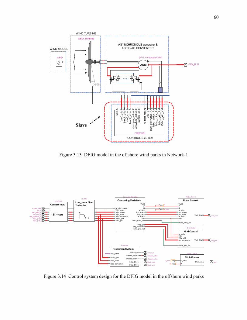
60

Figure 3.13 DFIG model in the offshore wind parks in Network-1

Figure 3.14 Control system design for the DFIG model in the offshore wind parks

WIND TURBINE

WIND MODELASYNCHRONOUS generator & AC/DC/AC CONVERTER

CONTROL SYSTEM

GEN_BUS

WIND

beta

WIND_TURBINE

ASM

DFIG_hardw areAVM1

pitc

h

crow

bar_

activ

e

w_ro

tor_

rads

Vdc_

V

Vabc

_grid

_VIa

bc_g

rid_A

Iabc

_rot

or_A

Iabc

_sta

tor_

AIa

bc_c

onve

rter_

A

switc

h_on

chop

per_

activ

e

Vref

_rot

or

Vref

_grid

bloc

k_gr

id

bloc

k_ro

tor

CONTROL

switch_on

pitch

chopper_active

crowbar_active

Pagew_rotor

Vref_rotor

Vref_grid

block_rotor

block_grid

Vabc_grid_VIabc_grid_A

Iabc_rotor_AIabc_stator_A

Iabc_converter_A

Vdc_V

Protection System

chopper_activ e

switch_onVdc_meas

Vabc_gridcrowbar_activ e

Iabc_rotor

Iabc_conv erterRSC_blockGSC_block

Protection

Low_pass filter2nd order

LP_filter

PageP

Convert to pu

SI -> pu

conv_to_pu

w_rotor_rads

Computing Variables

theta_rotor_rad

w_rotor

Iabc_rotorIabc_stator

Iabc_conv erter

w_rotor_meas

Idq_conv erterVdq_grid

Idq_rotorIdq_stator

P

theta_grid_rad

Vabc_gridIabc_grid

Q

Vgrid

w_stator

Vdc_meas

Vdc

Computing_Variables

Page w_rotor

Page P

Grid Control

theta_grid_rad

Vref _PWMVdq_gridIdq_conv erter

Vdcw_stator

Grid_Control

Rotor Control

w_rotor

Vdc

theta_rotor_rad

Idq_statorIdq_rotor Vref _PWM

PQ

Vgrid

w_stator

Rotor_Control

Pitch Control

P

w_rotor Pitch_deg

Pitch_Control

Slave

61

The simulation interval is 3 s for all scenarios and the Original Case. The three-phase permanent

fault location is indicated in Figure 3.10 and occurs at 1t s= . The waveforms of average active

power and phase-a current flowing out of the offshore AC cable (of HVDC converter) into the grid

are presented in Figure 3.15. For better observation, only the interval between 0.75t s= and

1.25t s= is presented for both waveforms.

(a) Average active power

(b) Phase-a current

Figure 3.15 Waveforms of average active power and phase-a current

Upon closer inspection, it is observed that the maximum (all solution time-points) per-unit error in

all simulation scenarios in comparison to the Original Case is less than 0.01% , thus demonstrating

that the implementation of the FMI-based new simulation approach on the offshore wind park

controls remain accurate. An error analysis is provided in a later section.

62


This test case validates the accuracy of the FMI-based co-simulation approach in relay applications

by examining line relay tripping instants after a fault. It studies relay tripping events at adjacent

lines when a phase-to-ground fault occurs at a line whose own relays are defective hence could not

trip for fault clearance. The Network-2 benchmark is used in this test case (see Figure 3.18). It is a

realistic power system simulation benchmark based on the data of [92], [93]. This 459-bus

benchmark consists of 7 voltage levels (transmission, sub-transmission, distribution and

generation), 637 transmission lines represented by both CP models and PI sections, and 10 type-

III onshore wind generators connected at sub-transmission level. Parameter and modelling details

can be found in [88]. The total number of network nodes in this benchmark is 3407, with the size

of main network equations being 12120×12120 (125120 non-zeros). Two line relays are added to

every CP line in the benchmark, represented by the rectangular boxes (Figure 3.18) whose contents

are shown in Figure 3.16. Settings of Relay 1 related to this particular study are presented in Figure

3.17 for demonstration purposes. It is noted that each line relay contains 4893 control devices [94],

and the entire relay is decoupled from the electrical network as the slave subsystem in co-

simulation.

Figure 3.16 Line relay at each end of a CP line

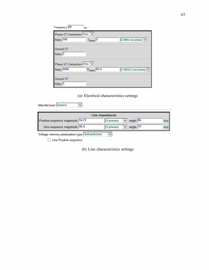
63

(a) Electrical characteristics settings

(b) Line characteristics settings

64

(c) Phase-to-ground distance settings, Zone 1

Figure 3.17 Relay 1 settings (partial)

65


1 W

F

2 W

Fs

1 W

F

3 W

Fs

2 W

F

1 W

F

CP+ 12

5.00

CP+ 14

7.00

CP+ 62

.00

CP+ 32

.00

CP+ 32

.00

CP+ 25

.00

CP+ 22

.00

CP+ 22

5.00

CP+ 87

.00

CP+ 87

.00

CP+ 66

.00

CP+ 13

6.00

CP+ 13

6.00

CP+ 17

2.00

CP+ 44

.00

CP+ 20

2.00

CP+20

6.00

CP+ 21

6.00

CP+ 10

0.00

+

5.745428803

Reactor_OSMAN

+

5.745428803

Reactor_CANKI

CP+ 34

.00

+

3.45

Reactor_SINCA

CP +

168.00

CP+

266.00

+9.

6458

e-00

5

C1_

UR

GU

P

+

9.64

58e-

005

C2_

UR

GU

PCP

+ 202.

00

CP+27

1.00

CP+ 27

1.00

+

9.09

46e-

005

C2_

KAYS

E

+

9.09

46e-

005

C1_

KAYS

E

CP+ 15

4.00

CP+ 10

9.00

CP+ 75

.00

CP+ 42

.00

CP+ 11

6.00

CP+ 18

6.00

+

9.64

58e-

005

C_E

RZI

N

+-1

|1E1

5|0

BYPA

SS

CP+80

.00

CP+ 35

0.00

+

9.64

58e-

005

C_S

EYD

I

CP+ 38

5.00

CP+ 85

.00

CP+ 65

.00

CP+ 82

.00

CP+ 46

.00

CP+ 28

7.00

CP +

182.00

CP +

146.00

CP+ 40

.00

CP+ 47

.00

YATA

G T

PP

YATA

G_T

PPYE

NIK

TPPYE

NIK

_TPP

KEM

ER

TPP

KEM

ER_T

PP

SOM

A T

PP

SOM

A_TP

P

SEYI

T T

PPSEYI

T_TP

P

TUNC

T

PP

TUN

C_T

PP

CAY

IR

TPP

CAY

IR_T

PP

LF

200MW100MVAR400kVRMSLL

Load_SEYDI

HAM

ITNG

CC

PP

HAM

IT_N

GC

CPP

CP+ 12

1.00

CP+ 17

0.00 EL

BIS

TPP

ELBI

S_TP

P

+

9.09

46e-

005

C1_

KAYA

B

+

9.09

46e-

005

C2_

KAYA

B+

9.09

46e-

005

C3_

KAYA

B

CP+ 16

7.00

CP+61

.00

KANG

A T

PP

KAN

GA_

TPP

CP+ 13

9.00

CP+ 27

1.00

CP+ 27

1.00

CP +

252.00CP +

85.00

CP +

85.00

+

3.45

Reactor_GOLBA

+ 2.3

Reactor_KAYSE

+

1.15

Reactor_KEBAN

+

6.964156125

Reactor_BABA

GO

KCE

HPP

GO

KCE_

HPP

OYM

AP H

PP

OYM

AP_H

PP

+

4.6

Reactor_SEYIT

+

2.3

Reactor_SEYDI

+

4.6

Reactor_ADANA

+

4.7

Reactor_KARAK

KARA

K H

PP

KAR

AK_H

PP

+ 2.3

L1

KEBA

N H

PP

KEBA

N_H

PP

+

1.15

Reactor_KAYAB

+

4.6

Reactor_URGUP

CP+

103.00

CP+

126.00

CP+ 95

.00

CP+ 19

.00

CP+ 19

.00

ALTI

N H

PP

ALTI

N_H

PPHU

GUR

HPP

HU

GU

R_H

PP

PI+

T

SB

BTS

BTS

SB

SB

SB

HC

HC

HC

H

H

YKYT

YY

CH

CH

CH

UG

UG

UG

H

AL10

0

H EL10

0

H CAY

100

H OY1

00

HER50

H

KAR

50

H KEB5

0

LF

Load_EREGL

100MW50MVAR400kVRMSLL

H CAN

50

HAD

A150

H AN20

0

UG

SG

SG

SK

SK

IA

AI

AI

OA

AO

AO

Out

InOu

tIn

Out

InOu

tIn

Out

In

OutIn

Out

In

OutIn

Out

InOut

In

OutIn

OutIn

Out

InOu

tIn

Out

InOu

tIn

Out

InOu

tIn

Out

InOu

tIn

Out

InOu

tIn

Out

InOu

tIn

Out

InOu

tIn

Out

InOu

tIn

Out

InOu

tIn

Out

InOu

tIn

Out

InOu

tInOu

tIn

OutIn

Out

InOu

tIn

Out

InOu

tIn

Out

In

OutIn

Out

InOu

tInOu

tIn

OutIn

OutIn

Out

In

Out

In

OutIn

H K100

Out

InOu

tIn

Out

InOu

tIn

Out

In Out

In

OutIn

OutIn

Out

In

OutIn

Out

In

Out

InOu

tInOu

tIn

OutIn

Out

InOu

tIn

Out

InOu

tIn

Out

InOu

tInOu

tIn

Out

In

Out

InOu

tIn

Out

In Out

In

OutIn

OutIn

Out

InOu

tIn

Out

InOu

tIn

Out

InOu

tIn

Out

InOu

tIn

Out

InOu

tIn

Out

In

OutIn

Out

InOu

tInOu

tIn

OutIn

Out

InOu

tIn

Out

InOu

tInOu

tIn

OutIn

Out

InOu

tInOu

tIn

OutIn

Out

InOu

tInOu

tIn

OutIn

Out

InOu

tInOu

tIn

OutIn

Out

In

OutIn

OutIn

BABA

CAN

KI

KAN

GA

OYM

AP

ADAN

A

SIVA

S

KEM

ER

TUN

C

SOM

ABA

LIK

UM

RAN

GEB

ZE

EREG

L

ALIA

G

CB_

GO

KCE

YEN

IKYA

TAG

IZM

IR

BUR

SA

SEYI

T

CB_

ADAP

A

SEYD

I

ERZI

N

ANTE

P

ELBI

SKA

RAK

KEBA

N

KAYS

E

HAM

IT

CO

P

CAY

IR

SIN

CA

GO

LBA

HAL

KAO

SMAN

KAYA

B

ALTI

NC

ARSA

HU

GU

R

UR

GU

P

Relay 1 Relay 2 Relay 3

Relay 4 Relay 5

Defective Faulty line

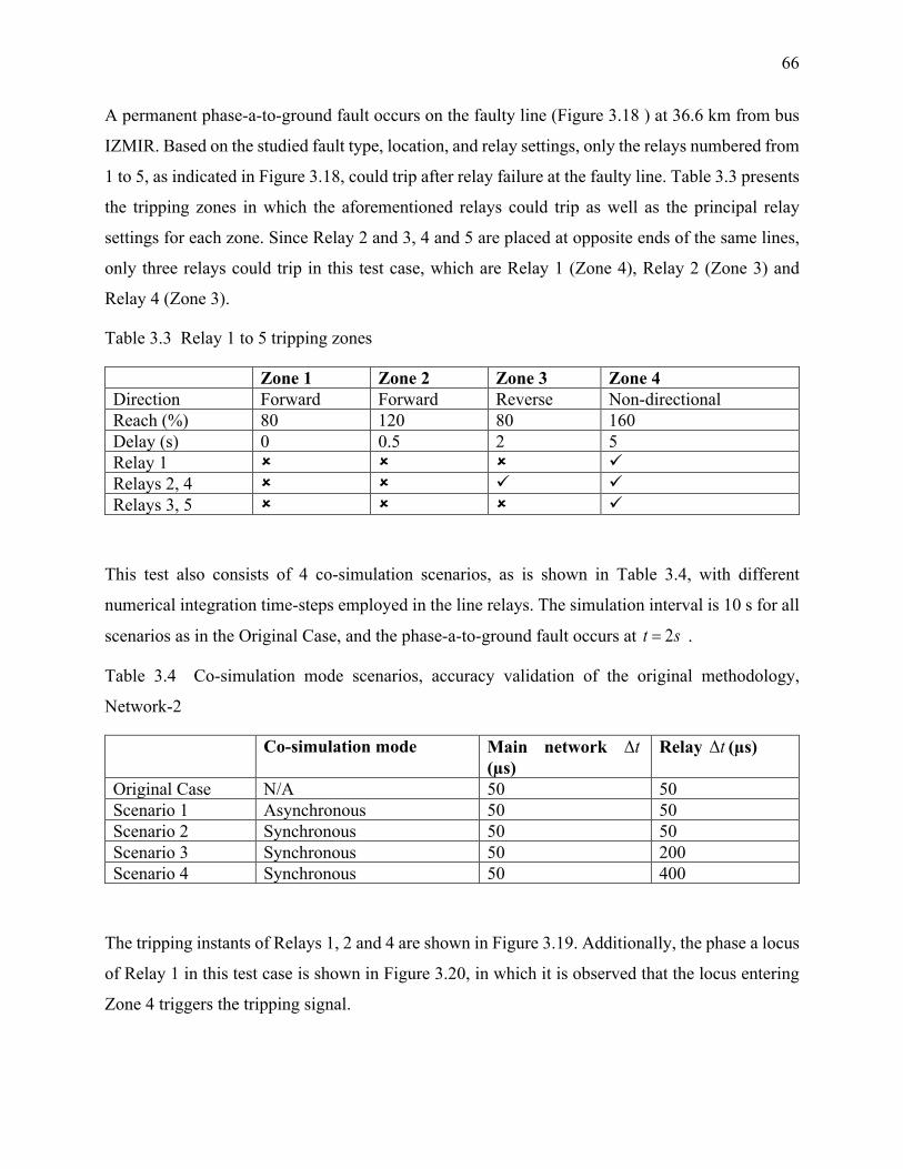
66

A permanent phase-a-to-ground fault occurs on the faulty line (Figure 3.18 ) at 36.6 km from bus

IZMIR. Based on the studied fault type, location, and relay settings, only the relays numbered from

1 to 5, as indicated in Figure 3.18, could trip after relay failure at the faulty line. Table 3.3 presents

the tripping zones in which the aforementioned relays could trip as well as the principal relay

settings for each zone. Since Relay 2 and 3, 4 and 5 are placed at opposite ends of the same lines,

only three relays could trip in this test case, which are Relay 1 (Zone 4), Relay 2 (Zone 3) and

Relay 4 (Zone 3).

Table 3.3 Relay 1 to 5 tripping zones

Zone 1 Zone 2 Zone 3 Zone 4 Direction Forward Forward Reverse Non-directional Reach (%) 80 120 80 160 Delay (s) 0 0.5 2 5 Relay 1 Relays 2, 4 Relays 3, 5

This test also consists of 4 co-simulation scenarios, as is shown in Table 3.4, with different

numerical integration time-steps employed in the line relays. The simulation interval is 10 s for all

scenarios as in the Original Case, and the phase-a-to-ground fault occurs at 2t s= .


Network-2


Relay t∆ (µs)

Original Case N/A 50 50 Scenario 1 Asynchronous 50 50 Scenario 2 Synchronous 50 50 Scenario 3 Synchronous 50 200 Scenario 4 Synchronous 50 400

The tripping instants of Relays 1, 2 and 4 are shown in Figure 3.19. Additionally, the phase a locus

of Relay 1 in this test case is shown in Figure 3.20, in which it is observed that the locus entering

Zone 4 triggers the tripping signal.

67

(a) Relay 1 tripping in Zone 4

(b) Relay 2 tripping in Zone 3

(c) Relay 4 tripping in Zone 3

Figure 3.19 Tripping instants of Relays 1, 2 and 4

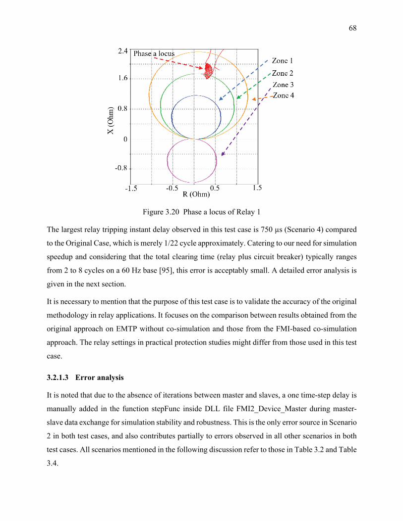
68

Figure 3.20 Phase a locus of Relay 1

The largest relay tripping instant delay observed in this test case is 750 µs (Scenario 4) compared

to the Original Case, which is merely 1/22 cycle approximately. Catering to our need for simulation

speedup and considering that the total clearing time (relay plus circuit breaker) typically ranges

from 2 to 8 cycles on a 60 Hz base [95], this error is acceptably small. A detailed error analysis is

given in the next section.

It is necessary to mention that the purpose of this test case is to validate the accuracy of the original

methodology in relay applications. It focuses on the comparison between results obtained from the

original approach on EMTP without co-simulation and those from the FMI-based co-simulation

approach. The relay settings in practical protection studies might differ from those used in this test

case.

3.2.1.3 Error analysis

It is noted that due to the absence of iterations between master and slaves, a one time-step delay is

manually added in the function stepFunc inside DLL file FMI2_Device_Master during master-

slave data exchange for simulation stability and robustness. This is the only error source in Scenario

2 in both test cases, and also contributes partially to errors observed in all other scenarios in both

test cases. All scenarios mentioned in the following discussion refer to those in Table 3.2 and Table

3.4.

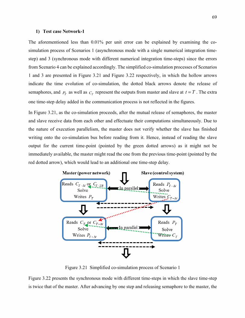
69

1) Test case Network-1

The aforementioned less than 0.01% per unit error can be explained by examining the co-

simulation process of Scenarios 1 (asynchronous mode with a single numerical integration time-

step) and 3 (synchronous mode with different numerical integration time-steps) since the errors

from Scenario 4 can be explained accordingly. The simplified co-simulation processes of Scenarios

1 and 3 are presented in Figure 3.21 and Figure 3.22 respectively, in which the hollow arrows

indicate the time evolution of co-simulation, the dotted black arrows denote the release of

semaphores, and TP as well as TC represent the outputs from master and slave at t T= . The extra

one time-step delay added in the communication process is not reflected in the figures.

In Figure 3.21, as the co-simulation proceeds, after the mutual release of semaphores, the master

and slave receive data from each other and effectuate their computations simultaneously. Due to

the nature of execution parallelism, the master does not verify whether the slave has finished

writing onto the co-simulation bus before reading from it. Hence, instead of reading the slave

output for the current time-point (pointed by the green dotted arrows) as it might not be

immediately available, the master might read the one from the previous time-point (pointed by the

red dotted arrow), which would lead to an additional one time-step delay.

Figure 3.21 Simplified co-simulation process of Scenario 1

Figure 3.22 presents the synchronous mode with different time-steps in which the slave time-step

is twice that of the master. After advancing by one step and releasing semaphore to the master, the

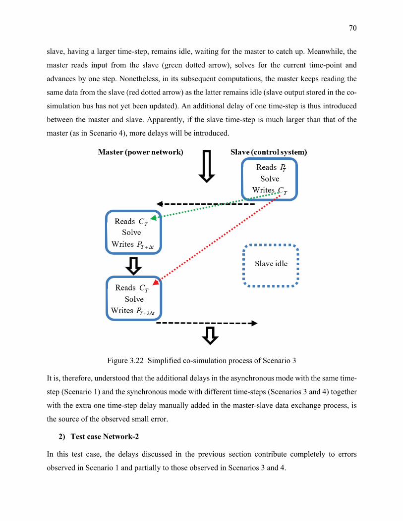
70

slave, having a larger time-step, remains idle, waiting for the master to catch up. Meanwhile, the

master reads input from the slave (green dotted arrow), solves for the current time-point and

advances by one step. Nonetheless, in its subsequent computations, the master keeps reading the

same data from the slave (red dotted arrow) as the latter remains idle (slave output stored in the co-

simulation bus has not yet been updated). An additional delay of one time-step is thus introduced

between the master and slave. Apparently, if the slave time-step is much larger than that of the

master (as in Scenario 4), more delays will be introduced.

Figure 3.22 Simplified co-simulation process of Scenario 3

It is, therefore, understood that the additional delays in the asynchronous mode with the same time-

step (Scenario 1) and the synchronous mode with different time-steps (Scenarios 3 and 4) together

with the extra one time-step delay manually added in the master-slave data exchange process, is

the source of the observed small error.

2) Test case Network-2

In this test case, the delays discussed in the previous section contribute completely to errors

observed in Scenario 1 and partially to those observed in Scenarios 3 and 4.

71

Another source of errors in Scenarios 3 and 4 (synchronous mode with different numerical

integration time-steps) is due to the interpolation process in relay sampling. The relay models used

in the work of this thesis require that the interval between sampling instants should be larger than

twice the relay numerical integration time-step [95]. For this reason, in Scenario 4 where the relay

time-step is 400 µs, a sampling rate of 20 samples/cycle is chosen, which renders an interval of

833.33 µs between sampling instants. Such an interval indicates that the relay sampling instants

are not on time mesh since the relay time-step is 400 µs and that of the main network is 50 µs. An

interpolation is thus performed at each sampling instant using data from the two adjacent relay

simulation time-points between which the sampling instant occurs [95]. As the interpolation for

relay sampling will not be performed until the data from a later simulation time-point becomes

available, a delay is, therefore, introduced, which also constitutes the observed errors in relay

tripping signals in Scenario 4. Errors in Scenario 3 can be explained in a similar fashion.

The largest errors are observed in Scenario 4 where a numerical integration time-step of 400 µs is

adopted in the relays. This is only for demonstrating application capacity of the proposed approach.

In practice, a smaller relay time-step can be used for higher simulation accuracy while obtaining

similar speedup, as will be seen in the following section.

3.2.2 Computation time gains

The validation of the original methodology in the aspect of computation time gains is based on the

comparison of the solution time of the benchmarks simulated on EMTP without co-simulation and

with the FMI-based co-simulation approach. Its objective is to demonstrate the numerical

performance advantages of the FMI-based new co-simulation approach on practical power system

networks of different levels of complexity, Network-1 and -2, as are shown in Figure 3.10 and

Figure 3.18 respectively. Two PCs with 2 and 16 cores (4 and 32 logical processors respectively),

whose hardware and software configurations are given in Table 3.5, are used in the tests of

computation time gains. Again, in all cases, a multiphase unbalanced load-flow solution is

performed for initializing the time-domain solution where a fault condition is simulated. A

simulation interval of 2 s is used in all tests.

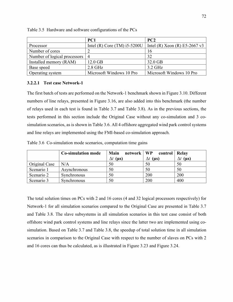
72

Table 3.5 Hardware and software configurations of the PCs

PC1 PC2 Processor Intel (R) Core (TM) i5-5200U Intel (R) Xeon (R) E5-2667 v3 Number of cores 2 16 Number of logical processors 4 32 Installed memory (RAM) 12.0 GB 32.0 GB Base speed 2.8 GHz 3.2 GHz Operating system Microsoft Windows 10 Pro Microsoft Windows 10 Pro


The first batch of tests are performed on the Network-1 benchmark shown in Figure 3.10. Different

numbers of line relays, presented in Figure 3.16, are also added into this benchmark (the number

of relays used in each test is found in Table 3.7 and Table 3.8). As in the previous sections, the

tests performed in this section include the Original Case without any co-simulation and 3 co-

simulation scenarios, as is shown in Table 3.6. All 4 offshore aggregated wind park control systems

and line relays are implemented using the FMI-based co-simulation approach.

Table 3.6 Co-simulation mode scenarios, computation time gains


WP control t∆ (µs)

Relay t∆ (µs)

Original Case N/A 50 50 50 Scenario 1 Asynchronous 50 50 50 Scenario 2 Synchronous 50 200 200 Scenario 3 Synchronous 50 200 400

The total solution times on PCs with 2 and 16 cores (4 and 32 logical processors respectively) for

Network-1 for all simulation scenarios compared to the Original Case are presented in Table 3.7

and Table 3.8. The slave subsystems in all simulation scenarios in this test case consist of both

offshore wind park control systems and line relays since the latter two are implemented using co-

simulation. Based on Table 3.7 and Table 3.8, the speedup of total solution time in all simulation

scenarios in comparison to the Original Case with respect to the number of slaves on PCs with 2

and 16 cores can thus be calculated, as is illustrated in Figure 3.23 and Figure 3.24.

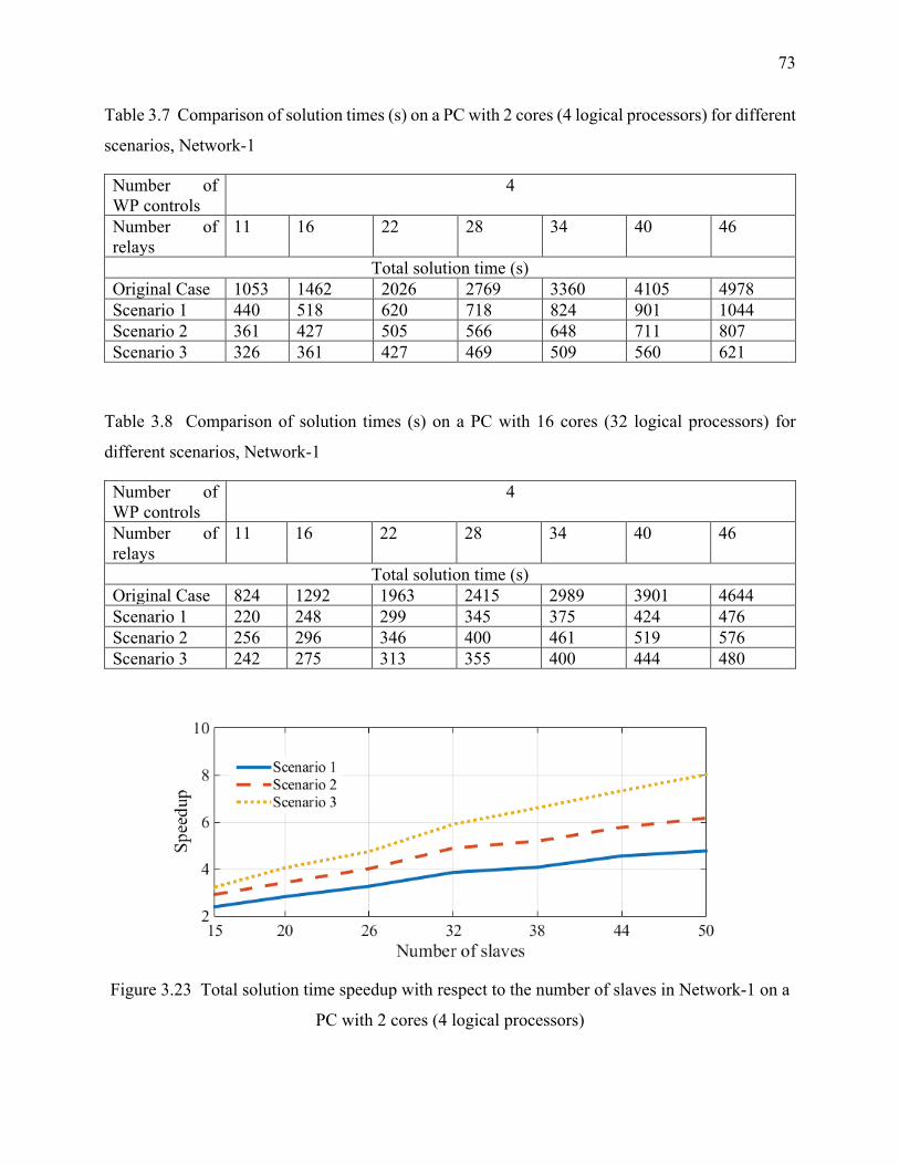
73


scenarios, Network-1

Number of WP controls

4

Number of relays

11 16 22 28 34 40 46

Total solution time (s) Original Case 1053 1462 2026 2769 3360 4105 4978 Scenario 1 440 518 620 718 824 901 1044 Scenario 2 361 427 505 566 648 711 807 Scenario 3 326 361 427 469 509 560 621


different scenarios, Network-1


4

Number of relays

11 16 22 28 34 40 46

Total solution time (s) Original Case 824 1292 1963 2415 2989 3901 4644 Scenario 1 220 248 299 345 375 424 476 Scenario 2 256 296 346 400 461 519 576 Scenario 3 242 275 313 355 400 444 480


PC with 2 cores (4 logical processors)

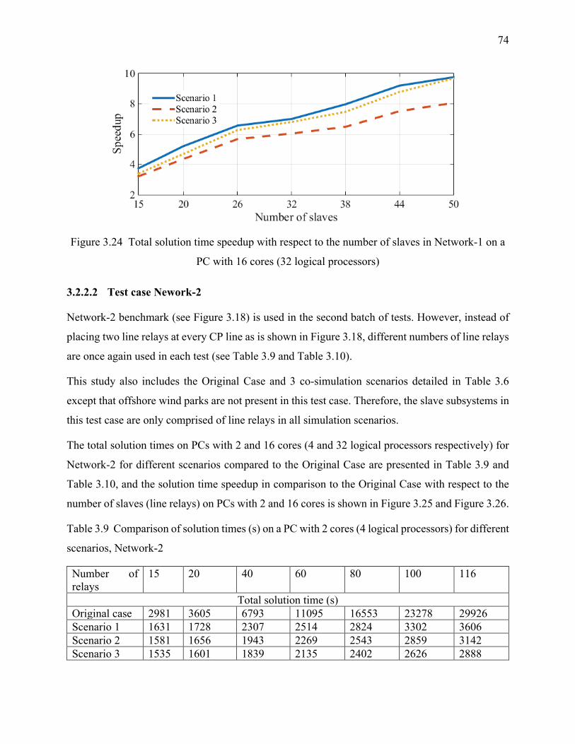
74



3.2.2.2 Test case Nework-2

Network-2 benchmark (see Figure 3.18) is used in the second batch of tests. However, instead of

placing two line relays at every CP line as is shown in Figure 3.18, different numbers of line relays

are once again used in each test (see Table 3.9 and Table 3.10).

This study also includes the Original Case and 3 co-simulation scenarios detailed in Table 3.6

except that offshore wind parks are not present in this test case. Therefore, the slave subsystems in

this test case are only comprised of line relays in all simulation scenarios.

The total solution times on PCs with 2 and 16 cores (4 and 32 logical processors respectively) for

Network-2 for different scenarios compared to the Original Case are presented in Table 3.9 and

Table 3.10, and the solution time speedup in comparison to the Original Case with respect to the

number of slaves (line relays) on PCs with 2 and 16 cores is shown in Figure 3.25 and Figure 3.26.


scenarios, Network-2

Number of relays

15 20 40 60 80 100 116

Total solution time (s) Original case 2981 3605 6793 11095 16553 23278 29926 Scenario 1 1631 1728 2307 2514 2824 3302 3606 Scenario 2 1581 1656 1943 2269 2543 2859 3142 Scenario 3 1535 1601 1839 2135 2402 2626 2888

75


different scenarios, Network-2

Number of relays

15 20 40 60 80 100 116

Total solution time (s) Original case 2419 2840 5494 9288 14426 19249 24351 Scenario 1 1237 1287 1471 1778 1939 2184 2563 Scenario 2 1259 1328 1492 1795 2091 2288 2601 Scenario 3 1246 1294 1418 1654 1862 2061 2263





76

Overall, it can be observed from Figure 3.23 to Figure 3.26 that considerable solution time speedup

is obtained in power system transient simulations using the new FMI-based co-simulation

approach. Furthermore, several conclusions on the comparison of the two co-simulation modes can

also be drawn as follows.

Firstly, since the computation of slave subsystems is distributed among separate logical processors

in both synchronous and asynchronous modes, as the number of decoupled slave subsystems

increases in a network, the solution time speedup in both modes increases accordingly, with the

computing capability of the multi-core CPU sufficiently exploited (see Figure 3.23 to Figure 3.26).

Secondly, in a computation environment where parallelism cannot be adequately fulfilled due to

limited available CPU cores, although executed sequentially, the synchronous mode could result

in a higher speedup compared to the asynchronous mode performed in parallel thanks to its

advantage of being able to adopt different time-steps in the control systems (see Figure 3.23 and

Figure 3.25).

Thirdly, the asynchronous mode could be more efficient than the synchronous mode with different

time-steps in achieving a higher speedup if the simulation can be parallelized among sufficient

logical processors (see Figure 3.24). However, its performance could still be surpassed by the

synchronous mode with different numerical integration time-steps in certain cases because of

communication overhead brought by data exchange between master and slaves at every time-point

in the parallel asynchronous mode (see the comparison between Scenarios 1 and 3 in Figure 3.26).

An in-depth analysis of the observed computation time gains in both co-simulation modes is

provided in the following section.

3.2.2.3 Discussion

This section elaborates on the computation time gains achieved using the FMI-based co-simulation

approach. The performance of both co-simulation modes (parallel asynchronous and sequential

synchronous) are analyzed for both test benchmarks (see Figure 3.23 and Figure 3.26) on two PCs

with 2 and 16 cores (4 and 32 logical processors respectively). The scenarios in the following

discussion refer to those in Table 3.6.

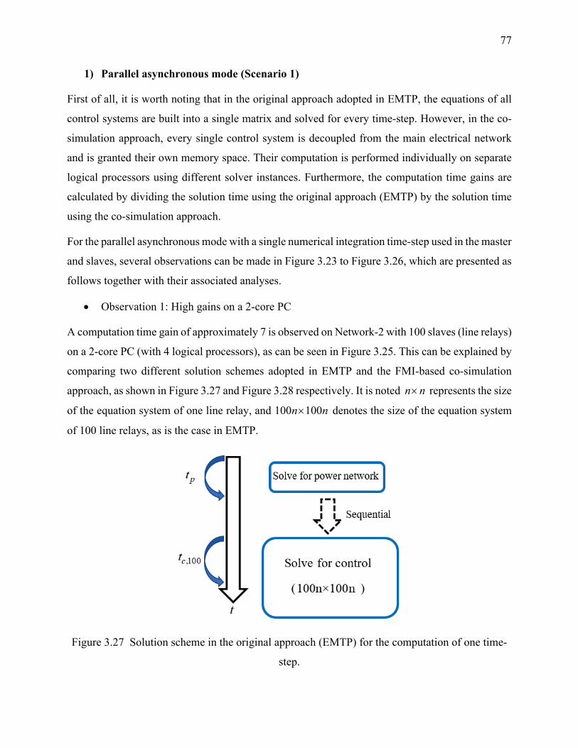
77

1) Parallel asynchronous mode (Scenario 1)

First of all, it is worth noting that in the original approach adopted in EMTP, the equations of all

control systems are built into a single matrix and solved for every time-step. However, in the co-

simulation approach, every single control system is decoupled from the main electrical network

and is granted their own memory space. Their computation is performed individually on separate

logical processors using different solver instances. Furthermore, the computation time gains are

calculated by dividing the solution time using the original approach (EMTP) by the solution time

using the co-simulation approach.

For the parallel asynchronous mode with a single numerical integration time-step used in the master

and slaves, several observations can be made in Figure 3.23 to Figure 3.26, which are presented as

follows together with their associated analyses.

• Observation 1: High gains on a 2-core PC

A computation time gain of approximately 7 is observed on Network-2 with 100 slaves (line relays)

on a 2-core PC (with 4 logical processors), as can be seen in Figure 3.25. This can be explained by

comparing two different solution schemes adopted in EMTP and the FMI-based co-simulation

approach, as shown in Figure 3.27 and Figure 3.28 respectively. It is noted n n× represents the size

of the equation system of one line relay, and 100 100n n× denotes the size of the equation system

of 100 line relays, as is the case in EMTP.

Figure 3.27 Solution scheme in the original approach (EMTP) for the computation of one time-

step.

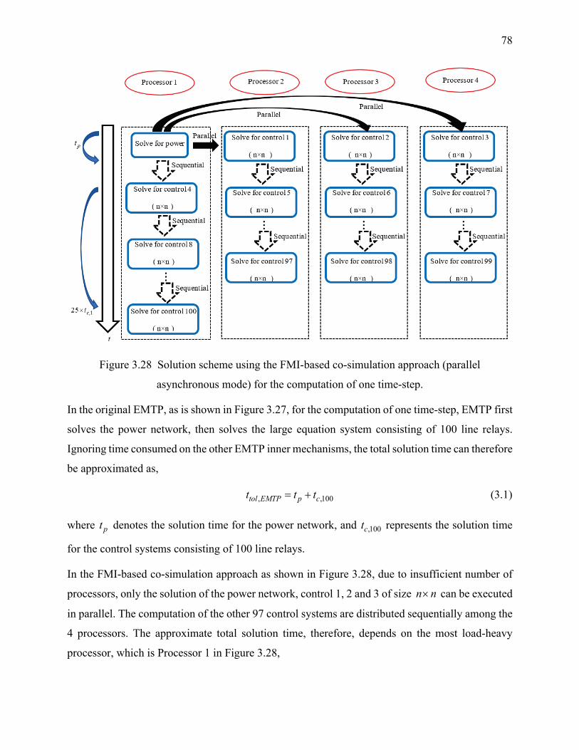
78

Figure 3.28 Solution scheme using the FMI-based co-simulation approach (parallel

asynchronous mode) for the computation of one time-step.

In the original EMTP, as is shown in Figure 3.27, for the computation of one time-step, EMTP first

solves the power network, then solves the large equation system consisting of 100 line relays.

Ignoring time consumed on the other EMTP inner mechanisms, the total solution time can therefore

be approximated as,

, ,100tol EMTP p ct t t= + (3.1)

where pt denotes the solution time for the power network, and ,100ct represents the solution time

for the control systems consisting of 100 line relays.

In the FMI-based co-simulation approach as shown in Figure 3.28, due to insufficient number of

processors, only the solution of the power network, control 1, 2 and 3 of size n n× can be executed

in parallel. The computation of the other 97 control systems are distributed sequentially among the

4 processors. The approximate total solution time, therefore, depends on the most load-heavy

processor, which is Processor 1 in Figure 3.28,

79

, ,125tol Co simulation p ct t t− = + × (3.2)

where ,1ct denotes the solution time for the control system consisting of one line relay. It is worth

mentioning that the computation load distribution among different processors is operating-system-

dependent in reality, and only one possibility is presented in Figure 3.28 for explanatory purposes.

Hence, the difference in solution times using both approaches lies in that: in EMTP, the equation

system of 100 relays is solved once, whereas in the FMI-based co-simulation approach, the

equation system of one individual relay is solved 25 times. Considering the arithmetic complexity

of sparse matrix solver for control systems used in the EMT-type solver [2], it is easy to deduce

that the former is considerably more time-consuming than the latter.

Based on the discussion above, it is understood why a gain larger than the number of processors

can be observed using the FMI-based co-simulation approach.

• Observation 2: Higher gains on a PC with more cores

From the test results on Network-1 (see Figure 3.23 and Figure 3.24) on PCs with different number

of processors, it is observed that for a specific number of slaves in the system, the gains on the 16-

core PC is higher than those on the 2-core PC. The reason is fairly straightforward: the more cores

(logical processors) there are in a PC, the more the computation load of individual control systems

is distributed. Each individual processor on a PC with more processors executes the solution of

fewer control systems. Hence, the total solution time of a benchmark with a specific number of

slaves is smaller on a PC with more processors.

• Observation 3: Higher gains on a benchmark with more slaves

It is observed on Network-2 on a 2-core PC (see Figure 3.25) that when the number of slaves

increases from 100 to 116, the gains jump from approximately 7.05 to 8.3. In both cases, the

number of decoupled slaves largely exceeds the number of available processors, so the computation

of most slaves is executed sequentially. The reason for such an observation is due to the fact that

in the original approach using EMTP, the extra time consumed to solve the equation system of 116

relays compared to solving that of 100 relays substantially exceeds the extra time for one processor

to sequentially solve the equation system of one individual relay 4 times (4 processors share the

computation load of the extra 16 relays in the FMI-based co-simulation approach) for reasons

80

elaborated in the explanation of Observation 1. This can also be seen in Table 3.9, of which only a

snippet is presented below in Table 3.11.

Table 3.11 Snippet of comparison of solution times (s) on a PC with 2 cores (4 logical processors)

for different scenarios, Network-2

Number of relays 100 116 EMTP (s) 23278 29926 FMI-based co-simulation (s) 3302 3606

As the number of slaves goes from 100 to 116, the total solution time using co-simulation increases

from 3302 s to 3606 s. However, using EMTP, the total solution time has seen a much higher jump

from 23278 s to 29926 s. Despite the slight increase in total solution time using co-simulation, the

computation time gains in the case of 116 relays are still higher.

• Observation 4: Higher gains on Network-1 than Network-2 for similar numbers of slaves

It is observed in Figure 3.24 that on the 16-core PC, Network-1 has a gain of 9.2 with 44 slaves (4

wind generators and 40 slaves) whereas the gain for Network-2 with 40 relays is barely 4 (see

Figure 3.26). This is due to the size difference between the two networks. For Network-1, the power

network equations are 4826×4826 with 35718 non-zeros, and the size of the power network

equations of Network-2 is 12120×12120 (125120 non-zeros). A major chunk of total solution time

is consequently spent on solving the power network in the case of Network-2. It can also be

observed for Network-2 with a specific number of slaves on the two different PCs, the gains on the

16-core PC are only slightly higher than those on the 2-core PC, indicating that a more distributed

computation load of individual control systems for Network-2 could not efficiently counter the

heavy solution burden brought by the large power network.

2) Sequential synchronous mode (Scenarios 2 and 3)

In this mode (Scenarios 2 and 3), a larger time-step is used in the control systems (slaves) whereas

the main electrical network (master) adopts a relatively smaller time-step. All the slaves are

individually solved once and remain idle while the master solves several times to catch up with the

slave time-point. In comparison to the original approach in EMTP where all control systems are

solved for every single time-step of the main electrical network, the computation time gain using

this mode is self-evident. A few observations can be still made, which are presented as follows

together with their associated analyses.

81

• Observation 1: Higher gains in scenarios with larger slave time-step

This is observed on all four figures from Figure 3.23 to Figure 3.26 (comparison between Scenarios

2 and 3). The larger the slave time-step is, the higher the gains are. This is due to the fact that the

larger the slave time-step is, the fewer the solutions of individual slaves are executed in the system

(more time being idle).

• Observation 2: Higher gains on a PC with more cores

This can be observed in all four figures from Figure 3.23 to Figure 3.26 for any specific number of

slaves. It is worth pointing out that in the synchronous mode, the computation of master and slaves

are performed sequentially. Nonetheless, there is no constraint with regards to the solution

sequence between slaves placed on separate processors as the slaves only communicate with the

master (not with each other). Therefore, this observation can be explained in the same fashion as

in Observation 2 of the parallel asynchronous mode.

Observations 3 and 4 for the parallel asynchronous mode can be made for the sequential multistep

synchronous mode as well. They can also be explained similarly here as in the parallel

asynchronous mode. It is also observed that the performance comparison of the parallel

asynchronous mode and the sequential multistep synchronous mode varies depending on the

number of slaves and the number of cores a PC has. In general, for a test benchmark such as

Network-1 with not many slaves (maximum 46 as in this test case), the parallel asynchronous mode

is more efficient than the sequential multistep synchronous mode thanks to solution parallelism (on

a 16-core PC with 32 logical processors); whereas for Network-2 on a 16-core PC, the performance

of the parallel asynchronous mode deteriorates when there are a sufficient number of slaves in the

system (from 100 to 116). This is because the number of individual decoupled slaves has far

exceeded the parallelization capacity of the PC, sequentially solving many control systems at every

single master time-step (parallel asynchronous mode) becomes, therefore, more time-consuming

than solving all control systems at a much larger slave time-step.

3.3 Validation of the improved methodology

In this section, tests validating the improved methodology, which is the parallel multistep

asynchronous mode and the linear extrapolation-based signal correction procedure proposed in

Section 2.3, are performed on power system simulation benchmarks with control systems of

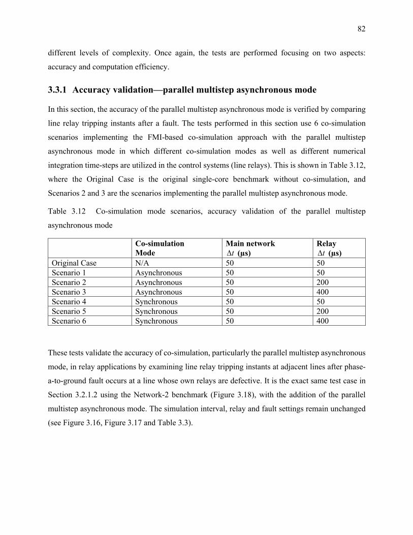
82

different levels of complexity. Once again, the tests are performed focusing on two aspects:

accuracy and computation efficiency.

3.3.1 Accuracy validation—parallel multistep asynchronous mode

In this section, the accuracy of the parallel multistep asynchronous mode is verified by comparing

line relay tripping instants after a fault. The tests performed in this section use 6 co-simulation

scenarios implementing the FMI-based co-simulation approach with the parallel multistep

asynchronous mode in which different co-simulation modes as well as different numerical

integration time-steps are utilized in the control systems (line relays). This is shown in Table 3.12,

where the Original Case is the original single-core benchmark without co-simulation, and

Scenarios 2 and 3 are the scenarios implementing the parallel multistep asynchronous mode.

Table 3.12 Co-simulation mode scenarios, accuracy validation of the parallel multistep

asynchronous mode

Co-simulation Mode

Main network t∆ (µs)

Relay t∆ (µs)

Original Case N/A 50 50 Scenario 1 Asynchronous 50 50 Scenario 2 Asynchronous 50 200 Scenario 3 Asynchronous 50 400 Scenario 4 Synchronous 50 50 Scenario 5 Synchronous 50 200 Scenario 6 Synchronous 50 400

These tests validate the accuracy of co-simulation, particularly the parallel multistep asynchronous

mode, in relay applications by examining line relay tripping instants at adjacent lines after phase-

a-to-ground fault occurs at a line whose own relays are defective. It is the exact same test case in

Section 3.2.1.2 using the Network-2 benchmark (Figure 3.18), with the addition of the parallel

multistep asynchronous mode. The simulation interval, relay and fault settings remain unchanged

(see Figure 3.16, Figure 3.17 and Table 3.3).

83

(a) Relay 1 tripping in Zone 4

(b) Relay 2 tripping in Zone 3

(c) Relay 4 tripping in Zone 3

Figure 3.29 Tripping instants of Relays 1, 2 and 4

84

The tripping instants of Relays 1, 2, and 4 are shown in Figure 3.29. The largest relay tripping

instant delay observed in this test case is 850 µs (Relay 4 in Scenario 3 using the parallel multistep

asynchronous mode) compared to the Original Case, which is approximately 1/19.6 cycle.

Although this error is slightly larger than those in the scenarios proposed in the original

methodology, it is still acceptably small catering to our need for simulation speedup and

considering that the total clearing time (relay plus circuit breaker) typically ranges from 2 to 8

cycles on a 60 Hz base [95], demonstrating that the use of different numerical integration time-

steps in different subsystems in the parallel multistep asynchronous mode does not affect accuracy.

3.3.2 Accuracy validation—linear extrapolation-based signal correction

In this section, the implementation of the linear extrapolation-based signal correction procedure on

floating-point type signals is validated in terms of accuracy improvement. Two new benchmarks

of different levels of complexity are used in the tests performed in this section. Again, all tests

involve several simulation scenarios implementing the FMI-based co-simulation approach with

different co-simulation modes as well as numerical integration time-steps. The test results with the

implementation of the linear extrapolation-based signal correction procedure are presented in

comparison with those without such a procedure. All test results are compared with the original

single-core benchmark on EMTP without co-simulation for reference.


This test is performed on the benchmark shown in Figure 3.30. It is a simple 5-bus 12.5 kV system

with one three-phase voltage source modeled using control devices. Other network components

and device parameters can be seen in Figure 3.30. It uses 2 scenarios with different numerical

integration time-steps used in the three-phase voltage source, as is shown in Table 3.13 in which

the Original Case is the original single-core benchmark without co-simulation.


signal correction procedure, Network-3

Co-simulation mode

Main network t∆ (µs)

Source t∆ (µs)

Original Case N/A 10 10 Scenario 1 Synchronous 10 50 Scenario 2 Synchronous 10 100

85


The simulation interval is 1 s for all simulation scenarios. At 0.5t s= , breakers BR1 and BR2

open, shedding loads FdrLoad and Load4801 as well as transformers TRANSFO from the system.

In both scenarios, the three-phase voltage source is decoupled from the electrical network to form

the slave subsystem.

Figure 3.31 and Figure 3.32 present the phase-b voltage at bus XFMR in the Original Case and

both co-simulation scenarios without and with signal extrapolation respectively. For clear

observation, only the interval between 0.5t s= and 0.55t s= after circuit breaker operation is

shown in Figure 3.31 (a) and Figure 3.32 (a).

+Rd

50

PI+ Z1

CP+

TLM1

125.00

+BRk

-1|1E15|0

P Q Load2

0.48kVRMSLLP=400kWQ=193.729kVAR

+BR2

-1|0.5|0

P QLoad4801

0.48kVRMSLLP=400MWQ=0MVAR

12-3

0

DYg_112.5/0.48

12-3

0

TRANSFO12.5/0.48

PQ

FdrLoad

12.5kVRMSLLP=1MWQ=0.25MVAR

+BR1

-1|0.5|0

+BRm

-1|1E15|0

+

12.5kVRMSLL /_0

AC

BUS1

BUS2 4801

XFMRBUS_SOURCE

Slave

86

(a) Overall waveforms

(b) Waveforms in the amplified region

Figure 3.31 Phase-b voltage at bus XFMR between 0.5t s= and 0.55t s= without signal

correction with closer observation of waveforms in the amplified region

Amplified region

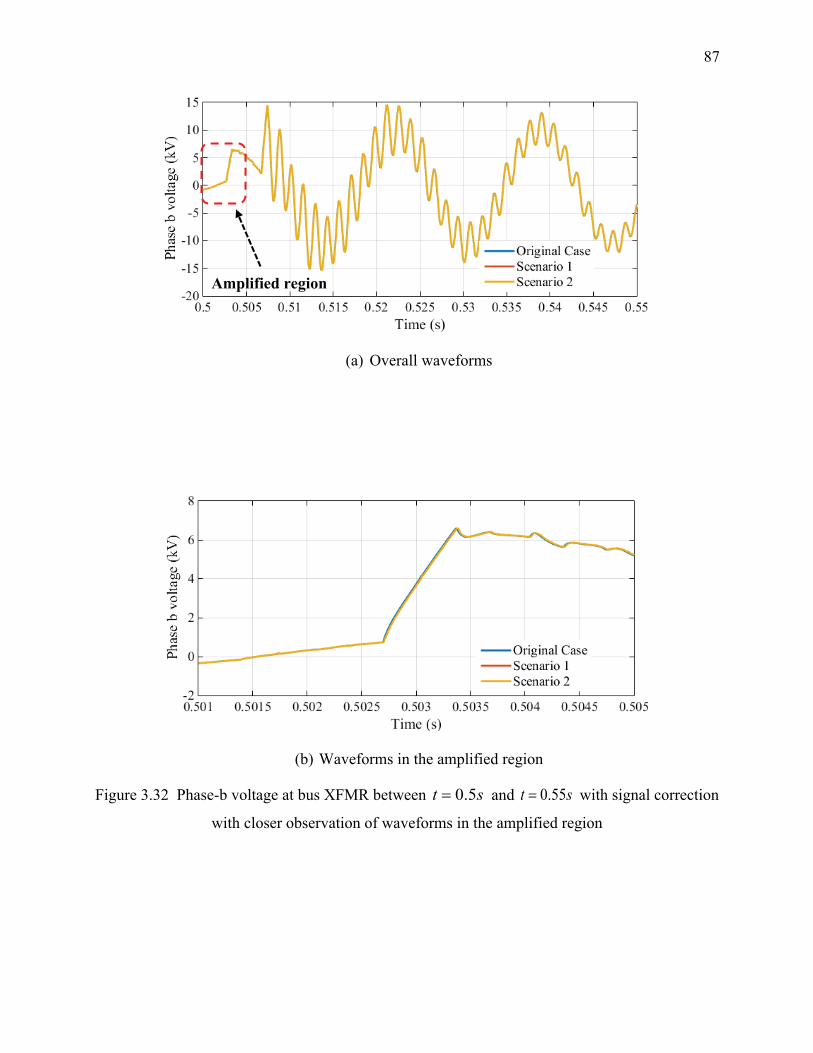
87

(a) Overall waveforms

(b) Waveforms in the amplified region

Figure 3.32 Phase-b voltage at bus XFMR between 0.5t s= and 0.55t s= with signal correction

with closer observation of waveforms in the amplified region

Amplified region

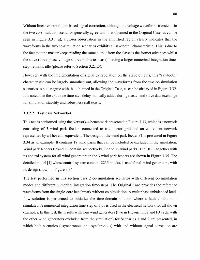
88

Without linear extrapolation-based signal correction, although the voltage waveforms transients in

the two co-simulation scenarios generally agree with that obtained in the Original Case, as can be

seen in Figure 3.31 (a), a closer observation in the amplified region clearly indicates that the

waveforms in the two co-simulation scenarios exhibits a “sawtooth” characteristic. This is due to

the fact that the master keeps reading the same output from the slave as the former advances whilst

the slave (three-phase voltage source in this test case), having a larger numerical integration time-

step, remains idle (please refer to Section 3.2.1.3).

However, with the implementation of signal extrapolation on the slave outputs, this “sawtooth”

characteristic can be largely smoothed out, allowing the waveforms from the two co-simulation

scenarios to better agree with that obtained in the Original Case, as can be observed in Figure 3.32.

It is noted that the extra one time-step delay manually added during master and slave data exchange

for simulation stability and robustness still exists.


This test is performed using the Network-4 benchmark presented in Figure 3.33, which is a network

consisting of 3 wind park feeders connected to a collector grid and an equivalent network

represented by a Thevenin equivalent. The design of the wind park feeder F1 is presented in Figure

3.34 as an example. It contains 18 wind parks that can be included or excluded in the simulation.

Wind park feeders F2 and F3 contain, respectively, 12 and 15 wind parks. The DFIG together with

its control system for all wind generators in the 3 wind park feeders are shown in Figure 3.35. The

detailed model [1] whose control system contains 2235 blocks, is used for all wind generators, with

its design shown in Figure 3.36.

The test performed in this section uses 2 co-simulation scenarios with different co-simulation

modes and different numerical integration time-steps. The Original Case provides the reference

waveforms from the single-core benchmark without co-simulation. A multiphase unbalanced load-

flow solution is performed to initialize the time-domain solution where a fault condition is

simulated. A numerical integration time-step of 5 µs is used in the electrical network for all shown

examples. In this test, the results with four wind generators (two in F1, one in F2 and F3 each, with

the other wind generators excluded from the simulation) for Scenarios 1 and 2 are presented, in

which both scenarios (asynchronous and synchronous) with and without signal correction are

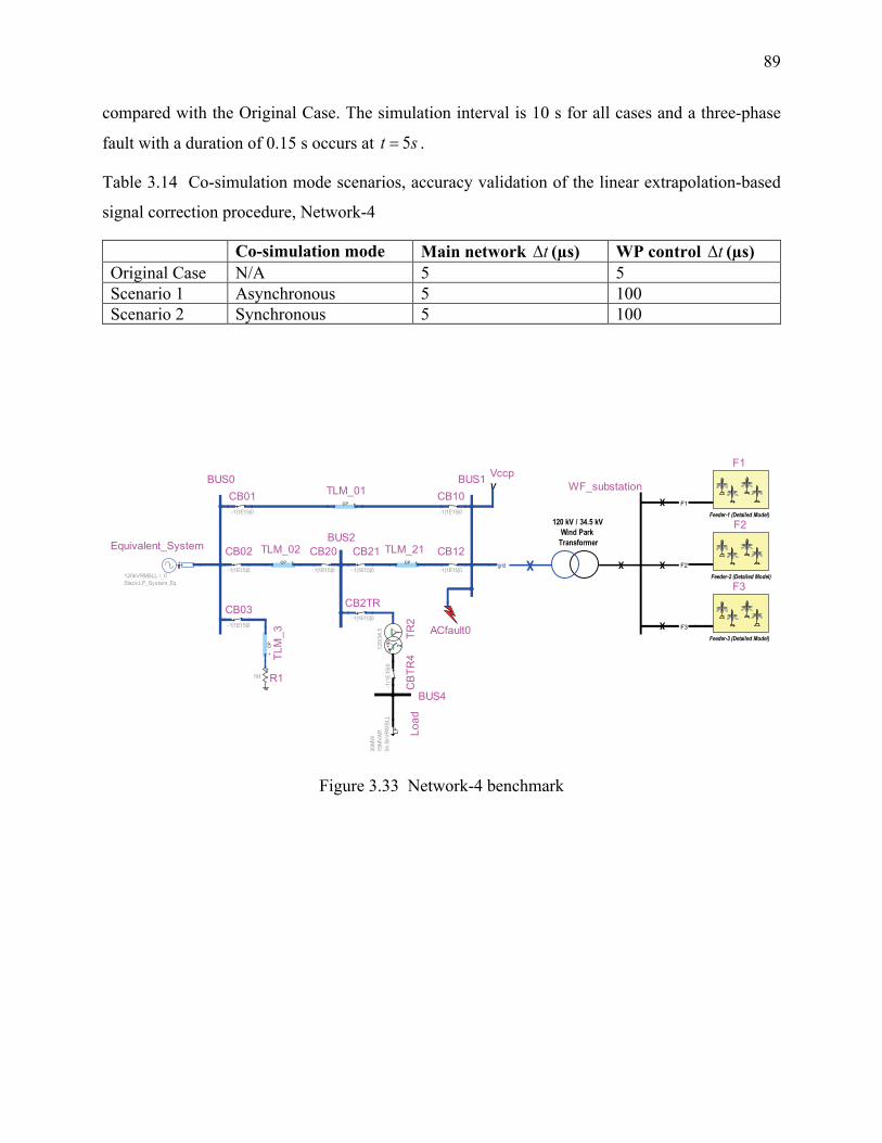
89

compared with the Original Case. The simulation interval is 10 s for all cases and a three-phase

fault with a duration of 0.15 s occurs at 5t s= .


signal correction procedure, Network-4

Co-simulation mode Main network t∆ (µs) WP control t∆ (µs) Original Case N/A 5 5 Scenario 1 Asynchronous 5 100 Scenario 2 Synchronous 5 100


VVccp

+

Equivalent_System

120kVRMSLL /_0 Slack:LF_System_Eq

12+3

0

TR2

120/

34.5

LF Load

30M

W15

MVA

R34

.5kV

RM

SLL

CP

+ TLM

_3

+

R11M

CP +

TLM_21CP +

TLM_02

CP +

TLM_01 X

X

X

XX

120 kV / 34.5 kV Wind Park Transformer

F3

F2

F1

grid

WF_substation

Feeder-2 (Detailed Model)

F2


F3


F1

+-1|1E15|0

CB01

+-1|1E15|0

CB02

+-1|1E15|0

CB03

+-1|1E15|0

CB10

+-1|1E15|0

CB20+

-1|1E15|0

CB21+

-1|1E15|0

CB12

+-1|1E15|0

CB2TR

+-1

|1E1

5|0

CBT

R4

ACfault0

BUS0

BUS2

BUS4

BUS1

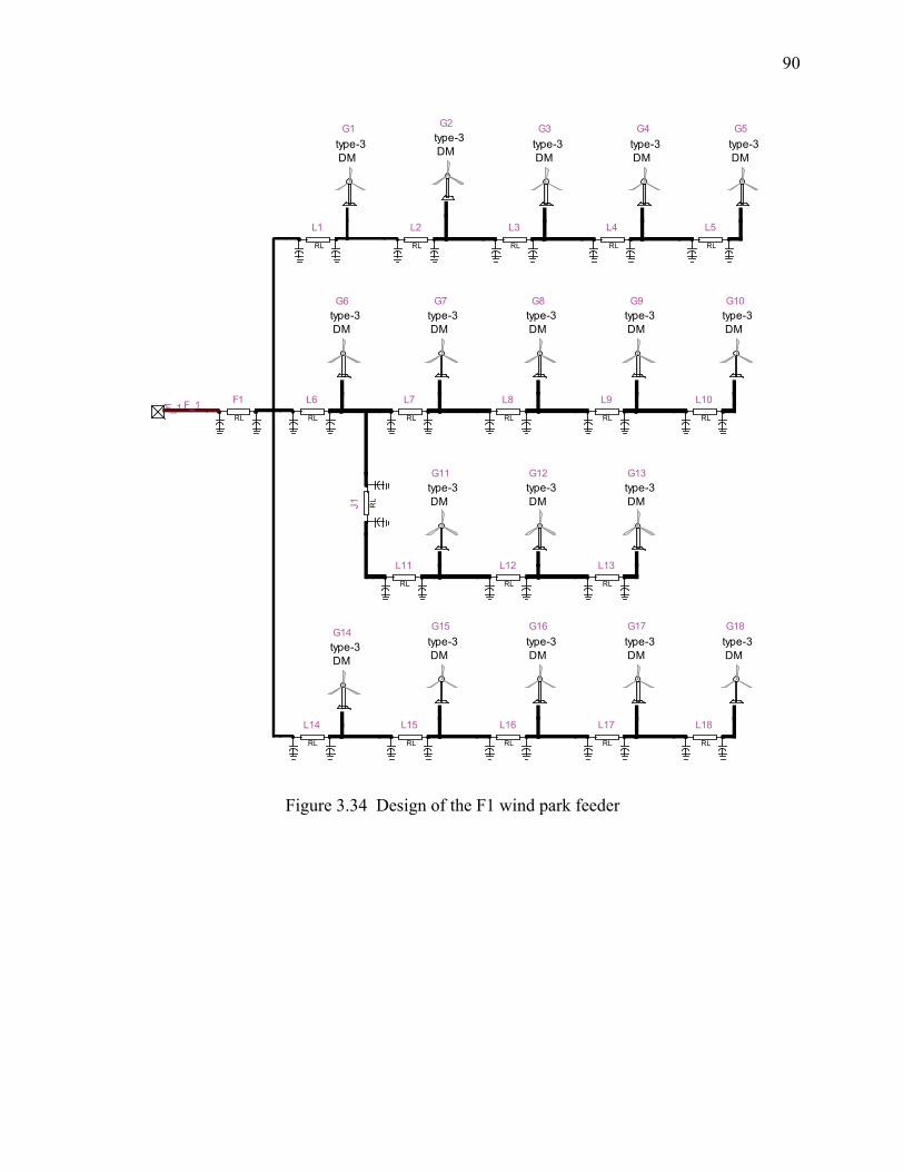
90

Figure 3.34 Design of the F1 wind park feeder

RL

F1

RL

L1

RL

L2

RL

L3

RL

L4

RL

L5

RL

L6

RL

L7

RL

L8

RL

L9

RL

L10

RL

L12

RL

L13

RLJ1

RL

L11

RL

L14

RL

L15

RL

L16

RL

L17

RL

L18

F_1

type-3 DM

G1type-3 DM

G2

type-3 DM

G3type-3 DM

G4type-3 DM

G5

type-3 DM

G6type-3 DM

G7type-3 DM

G8type-3 DM

G9type-3 DM

G10

type-3 DM

G11type-3 DM

G12type-3 DM

G13

type-3 DM

G14type-3 DM

G15type-3 DM

G16type-3 DM

G17type-3 DM

G18

F_1

91

Figure 3.35 DFIG model with wind generator control systems modelled using the detailed model

Figure 3.36 Control system design for the DFIG model in the wind generator

The average active power from the three feeders and the phase-a voltage at the 34.5 kV bus, are

presented in Figure 3.37 and Figure 3.38 with clear observation in amplified intervals.

WIND TURBINE

HARDWARE EXCEPT AC/DC/AC CONVERTER

AC/DC/AC CONVERTER

DFIG CONTROL

PCC

DFIG

Ctrl

Vref_RSC

Vref_GSC

Istator_A

Igrid_AVgrid_V

Irotor_A

Iconv_A

Pitch_deg

Udc_V

SW_ON

Crowbar_ON

Block_RSC

Block_GSC

Chopper_ON

wgen_rad

dVref

Ctrl

RL

EqCollectorGrid1

v i

VIabc_POI

c

tap

#T_wp_tr#

c

#Mean_wind_speed#

v i

VIabc_mv

Page Vmv

Page Qmv

Page Qpoi

Page PmvPage Ppoi

Page Spoi

PageVmv

Page Vpoi

Page dUref

Page RV

PageSpoi

PageQpoi

PageVpoi

PageQmv

PageRV

PagedUref1

2

select

f(u)1 + (t > 0.4)

scopedUref

VmvQmv

RV

QpoiVpoi

VrefPFref

RC

QrefSpoiinitialize_WPCtrl

Vmv

Imv

PQ

Vmag_puVphase_rad

Imag_puIphase_rad

MV_meas

12

WindParkTransfo1

WPC

Vpoi

Ipoi

VrefQref

dUref

PFref

RCRV

PpoiQpoiVpoi

Spoi

WPCtrl

ASM

crow

bar

DFIG transformer

DFIG

beta

Wind_Turbine

Turbine IMmass-spring-damper system

Two_mass_model

B_to_B_converter1

use Vlv instead ofpredicted Vmv

Protection System

chopper_active

switch_onVdc_meas

Vabc_gridcrowbar_active

Iabc_rotorIabc_converter

RSC_blockGSC_block

Protection

Low_pass filter2nd order

LP_filter

Convert to pu

SI -> pu

conv_to_pu

Pitch Control

Pw_rotor Pitch_deg

Pitch_Control

Vref_RSC

Vref_GSC

Istator_A

Igrid_AVgrid_V

Irotor_AIconv_A

Pitch_deg

Udc_V

SW_ON

Crow bar_ON

Block_RSC

Block_GSC

Chopper_ON

w gen_rad

dVrefComputing Variables

theta_rotor_rad

w_rotor

Iabc_rotorIabc_stator

Iabc_converter

w_rotor_meas

Idq_converterVdq_grid

Idq_rotorIdq_stator

P

theta_grid_rad

Vabc_gridIabc_grid

w_stator

Vdc_meas

Vdc

predicted_VmvVlv

Q

Comput_Variables1

Grid Control

theta_grid_rad

Vref_PWMVdq_gridIdq_converter

Vdcw_statorVmvVlv

Grid_Control

Rotor Control

w_rotor

Vdctheta_rotor_rad

Idq_statorIdq_rotor Vref_PWM

P

w_stator

predicted_Vmv

dVrefVlv

Q

Rotor_Control

Slave

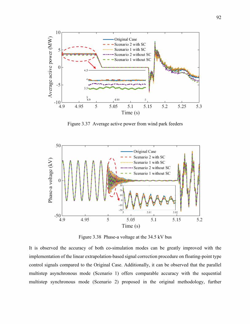
92

Figure 3.37 Average active power from wind park feeders

Figure 3.38 Phase-a voltage at the 34.5 kV bus

It is observed the accuracy of both co-simulation modes can be greatly improved with the

implementation of the linear extrapolation-based signal correction procedure on floating-point type

control signals compared to the Original Case. Additionally, it can be observed that the parallel

multistep asynchronous mode (Scenario 1) offers comparable accuracy with the sequential

multistep synchronous mode (Scenario 2) proposed in the original methodology, further

93

demonstrating that the implementation of the parallel multistep asynchronous mode does not affect

accuracy.

Overall, it can be concluded that better simulation accuracy can be achieved by the implementation

of floating-point type signal extrapolation in a multistep simulation environment.

3.3.3 Computation time gains

The objective of this section is to demonstrate the numerical performance advantages of the parallel

multistep asynchronous mode proposed in the improved methodology on practical power system

networks of different levels of complexity by comparing results obtained from benchmarks using

the FMI-based co-simulation approach (including the parallel multistep asynchronous mode) with

those using the single-core benchmarks on EMTP without co-simulation. Network-1, -2 and -4,

shown in Figure 3.10, Figure 3.18, and Figure 3.33 respectively, are used as test benchmarks. Once

again, a multiphase unbalanced load-flow solution is performed prior to time-domain simulation

where a fault condition is simulated. A simulation interval of 2 s is used in all test cases.


The tests performed in this section include the Original Case without co-simulation and 5 co-

simulation scenarios (see Table 3.15) implementing the parallel multistep asynchronous mode

(Scenarios 2 and 3) on benchmark Network-1 (see Figure 3.10), where different co-simulation

modes and numerical integration time-steps are employed in the control systems (offshore wind

generator controls and line relays). The tests are performed on the 16-core PC whose hardware and

software configurations are given in Table 3.5.


asynchronous mode, Network-1 and -2


WP control t∆ (µs)

Relay t∆ (µs)

Original Case N/A 50 50 50 Scenario 1 Asynchronous 50 50 50 Scenario 2 Asynchronous 50 200 200 Scenario 3 Asynchronous 50 200 400 Scenario 4 Synchronous 50 200 200 Scenario 5 Synchronous 50 200 400

94

Similar to the tests on computation time gains of the original methodology, different numbers of

line relays, presented in Figure 3.16, are added into this benchmark (see Table 3.16). The slave

subsystems in this test case thus consist of all 4 offshore aggregated wind generator control systems

(average model, see [1]) and line relays implemented using co-simulation in all scenarios.

The total solution time for Network-1 in different scenarios compared to the Original Case are

presented in Table 3.16, and the solution time speedup in comparison to the Original Case with

respect to the number of slaves (offshore wind generator controls and line relays) is shown in Figure

3.39.


Network-1, improved methodology


4

Number of relays

11 16 22 28 34 40 46

Total solution time (s) Original Case 824 1292 1963 2415 2989 3901 4644 Scenario 1 220 248 299 345 375 424 476 Scenario 2 223 246 284 313 348 382 414 Scenario 3 213 239 270 303 330 359 387 Scenario 4 256 296 346 400 461 519 576 Scenario 5 242 275 313 355 400 444 480


16-core PC, improved methodology

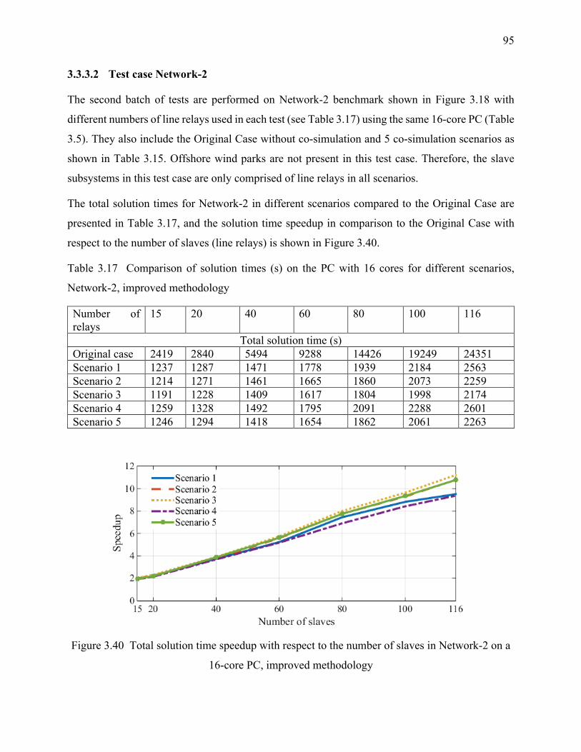
95


The second batch of tests are performed on Network-2 benchmark shown in Figure 3.18 with

different numbers of line relays used in each test (see Table 3.17) using the same 16-core PC (Table

3.5). They also include the Original Case without co-simulation and 5 co-simulation scenarios as

shown in Table 3.15. Offshore wind parks are not present in this test case. Therefore, the slave

subsystems in this test case are only comprised of line relays in all scenarios.

The total solution times for Network-2 in different scenarios compared to the Original Case are


respect to the number of slaves (line relays) is shown in Figure 3.40.


Network-2, improved methodology

Number of relays

15 20 40 60 80 100 116

Total solution time (s) Original case 2419 2840 5494 9288 14426 19249 24351 Scenario 1 1237 1287 1471 1778 1939 2184 2563 Scenario 2 1214 1271 1461 1665 1860 2073 2259 Scenario 3 1191 1228 1409 1617 1804 1998 2174 Scenario 4 1259 1328 1492 1795 2091 2288 2601 Scenario 5 1246 1294 1418 1654 1862 2061 2263



96


The tests performed in this section use the Original Case without co-simulation and 5 new co-

simulation scenarios, as is shown in Table 3.19, on the Network-4 benchmark presented in Figure

3.33. A numerical integration time-step of 5 µs is used in the electrical network for all shown

examples. A 24-core PC is used in these tests, with its hardware and software configurations given

in Table 3.18. It is noted that different numbers of wind generators (slaves) are used in the three

feeders to test the numerical performance and scalability of parallel multistep asynchronous mode

in the improved methodology. The exact numbers of wind generators used in this test case can be

seen in Table 3.20.

The total solution times for Network-4 in different scenarios compared to the Original Case are


respect to the number of slaves (wind generator controls) is shown in Figure 3.41.

Table 3.18 Hardware and software configurations of the 24-core PC

Processor Intel (R) Xeon (R) E5-2650 v4 Number of cores 24 Number of logical processors 48 Installed memory (RAM) 32.0 GB Base speed 2.2 GHz Operating system Microsoft Windows 10 Pro


asynchronous mode, Network-4

Co-simulation mode WP control t∆ (µs) Original Case N/A 5 Scenario 1 Asynchronous 5 Scenario 2 Asynchronous 50 Scenario 3 Asynchronous 100 Scenario 4 Synchronous 50 Scenario 5 Synchronous 100

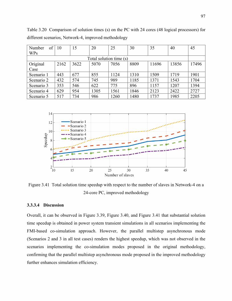
97

Table 3.20 Comparison of solution times (s) on the PC with 24 cores (48 logical processors) for

different scenarios, Network-4, improved methodology

Number of WPs

10 15 20 25 30 35 40 45

Total solution time (s) Original Case

2162 3622 5070 7056 8809 11696 13856 17496

Scenario 1 443 677 855 1124 1310 1509 1719 1901 Scenario 2 432 574 745 989 1185 1371 1543 1704 Scenario 3 353 546 622 775 896 1157 1207 1394 Scenario 4 629 954 1305 1561 1846 2123 2422 2727 Scenario 5 517 734 986 1260 1480 1737 1985 2205



3.3.3.4 Discussion

Overall, it can be observed in Figure 3.39, Figure 3.40, and Figure 3.41 that substantial solution

time speedup is obtained in power system transient simulations in all scenarios implementing the

FMI-based co-simulation approach. However, the parallel multistep asynchronous mode

(Scenarios 2 and 3 in all test cases) renders the highest speedup, which was not observed in the

scenarios implementing the co-simulation modes proposed in the original methodology,

confirming that the parallel multistep asynchronous mode proposed in the improved methodology

further enhances simulation efficiency.

98

Apart from the conclusions already drawn regarding the speedup achieved in different modes in

the discussion of computation time gains of the original methodology as well as the discussion in

Section 3.2.2.3, it is also worth mentioning that the results presented in Figure 3.39, Figure 3.40,

and Figure 3.41 do not clearly show speedup saturation although the number of decoupled

subsystems in some cases far exceeds the number of cores and logical processors of the PC. The

high scalability in the FMI-based co-simulation approach indicates even higher speedup could be

achieved in protection studies of large-scale networks using even more and different types of

protection relays and control systems.

3.4 Conclusion

This chapter presented simulation results using the FMI-based parallel and multistep approach

developed in this thesis. First of all, the design of the co-simulation interface on an EMT-type

solver [2] using the FMI standard was validated, establishing and confirming the platform for

further tests. Then both the original and the improved methodologies were validated for accuracy

and computation time gains using realistic power system simulation benchmarks with complex

control systems of different complexity, particularly wind generator controls and protection relays.

The tests performed using the original methodology demonstrated the numerical advantage of the

FMI-based co-simulation approach in terms of computation time gains while keeping the accuracy

properly maintained. The validation of the improved methodology testified to the numerical

performance enhancement in both accuracy control and solution speedup using the parallel

multistep asynchronous mode and the linear extrapolation-based signal correction.

99

CHAPTER 4 A PARALLEL-IN-TIME APPROACH BASED ON

PARALLEL-IN-TIME EQUATION GROUPING AND REORDERING

(PEGR)

This chapter presents the development of a new parallel-in-time approach implementing the

parallel-in-time equation grouping and reordering (PEGR) technique for power system EMT

simulations. The PEGR technique, originally proposed in [30], is a novel numerical solution

scheme that is formulated in state-space and could potentially formulate the solution by trapezoidal

integration for 2T τ= (τ is an integer) time-steps as a single problem involving T n× equations

and T n× unknowns ( n is the number of state variables). These equations can then be solved in

2log Tτ = steps using / 2T parallel processors. This technique is based on the identification of

truly independent tasks that could be performed simultaneously with an ideal number of parallel

processors after preprocessing procedures that consist of the construction of a huge matrix

containing the solutions at all time-points as well as a series of recursive row and column

reordering. Since building a huge matrix containing solutions at all time-points and solving it using

/ 2T parallel processors are unrealistic in practice due to the limitations of PC memory and the

number of available processors, this chapters focuses on adapting the PEGR technique to practical

power system EMT simulations on the base of modified-augmented-nodal analysis (MANA) [96]

which demonstrates several advantages over the conventional nodal analysis as well as state-space

formulation.

This chapter starts with a brief introduction of the modified-augmented-nodal analysis (MANA),

which is the theoretical base for the new parallel-in-time approach. It then explains in detail the

adaptation of the PEGR technique originally formulated in state-space to MANA through the

expansion of network equations. Subsequently, the equation grouping and recursive row and

column reordering scheme used in this new parallel-in-time approach as well as in the original

PEGR technique is demonstrated for a case in which the solutions of 16 time-steps are grouped.

Detailed programming considerations in the implementation of the PEGR-based parallel-in-time

approach are also discussed, including parallelization using OpenMP, measures adopted to

minimize concurrency issues in a parallel programming environment, block elements extraction

from L and U factors for backward and forward substitutions, , as well as treatment of arbitrary

points of topological changes and numbers of simulation points.

100

4.1 Formulation of the PEGR technique in MANA

In this section, a brief introduction of the modified-augmented-nodal analysis (MANA) used as the

theoretical base for the EMT-type solver [2] and the new parallel-in-time approach proposed in this

chapter is presented, followed by the adaptation of the original PEGR technique in MANA through

network equation expansion. The equation grouping and recursive row and column reordering

technique used in the new parallel-in-time approach as well as the original PEGR technique is then

explained in detail, using an example that groups the solutions of 16 time-steps. This is due to the

fact that the original PEGR technique formulates the solution by trapezoidal integration for 2T τ=

(τ is an integer) time-steps as a single problem, an example where 16 ( 416 2= ) time-steps are

grouped, reordered and solved would make it easy to understand this approach. The meaning of

“grouping” used in this chapter will become self-evident in the following discussions. The newly

proposed parallel-in-time approach and the original PEGR technique are general and can be used

to group the solutions of different numbers of time-steps, based on the computation capacity of the

PC.

4.1.1 Modified-augmented-nodal analysis (MANA)

The formulation of the parallel-in-time approach is based on the modified-augmented-nodal

analysis (MANA) formulation method [2]. This method offers several advantages [96] over

classical nodal analysis and state-space formulation. In MANA, the system of equations is generic

and can include different types of unknowns in addition to voltage. A brief introduction of the

MANA formulation is provided in this section. More details can be found in [2]. The general

MANA equations of a power system network can be written as,

Ax = b (4.1)

and can be expanded to,

A x bt t

n adj bdepc adj n n

Vadj ss

Vdbdepr

SWadj z

Y V D S V IIV 0 0 0 V

=0ID 0 0 00IS 0 0 S

(4.2)

101

where,

• nY is the linear network admittance matrix, non-symmetric

• adjV is the voltage source adjacency matrix, for all voltage source types

• bdeprD and bdepcD (row and column contribution matrices) are used for holding branch

dependent relations

• adjS is the adjacency matrix of closed switch type devices

• zS is a diagonal and unitary matrix for open switch type devices

• nV is the vector of unknown node voltages

• VsI is the vector of unknown voltage source currents

• VdI is the vector of unknown currents in dependent voltage source branches

• SWI is the vector of unknown switch currents

• nI is the vector of known nodal current injections

• sV is the vector of known voltage sources

Such an equation (4.1) can be used for both time-domain and steady-state solutions. It is a real

system in time-domain and a complex system in steady-state. Considering equation (4.1) is non-

symmetric and can also accommodate generic equations such as,

1 2 3 4 ...k m x y zk v k v k i k i b+ + + + = (4.3)

where the terms on the left contribute coefficients into the x matrix for voltage and current

unknowns, and zb is a cell in the b vector, other models, such as ideal transformers with tap

control can be also easily accommodated.

The sparse system of equations (4.1) is solved for x at each time-point in time-domain, after

updating the non-symmetric coefficient matrix A and the vector of known variables b . The vector

b contains history terms and other independent functions.

102

4.1.2 Expansion of network MANA equations

The thn order differential equation given in state-space,

( )x Ax f t= + (4.4)

with the initial condition,

( ) 00x x= (4.5)

can be rearranged using the trapezoidal rule into the form of,

( ) ( ) ( ) ( ) ( ) ( )2tx t t x t Ax t f t Ax t t f t t∆

+ ∆ = + + + + ∆ + + ∆ (4.6)

Equation (4.6) incorporates the solutions at two consecutive time-points ( )x t and ( )x t t+ ∆ ,

demonstrating the interdependency between solutions of consecutive time-points. This is the

foundation based on which the PEGR technique can be implemented [30].

In the original MANA formulation for power system networks, the history terms of energy storage

components such as inductors, capacitors and multiphase pi-sections are contained in b and are

updated for the calculation of each time-point in time-domain simulations, as was previously

explained. The solutions at two consecutive time-points are not directly formulated into one single

equation in MANA as in (4.6). Therefore, the PEGR technique cannot be directly implemented

into MANA formulation. The following discussion presents how to rearrange the network MANA

equations (4.1) into the form of (4.6) such that the equation grouping and recursive row and column

reordering scheme in PEGR can be applied, using multiphase pi-section as an example. Other

energy storage network components such as inductors and capacitors can be treated in a similar

fashion.

The generalized multiphase pi-section component connected between a set of left-hand nodes k

and right-hand nodes m is shown in Figure 4.1.

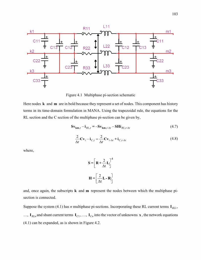
103

Figure 4.1 Multiphase pi-section schematic

Here nodes k and m are in bold because they represent a set of nodes. This component has history

terms in its time-domain formulation in MANA. Using the trapezoidal rule, the equations for the

RL section and the C section of the multiphase pi-section can be given by,

, , , - , -t RL t t t RL t t∆ ∆− − −km kmSv i = Sv SHi (4.7)

, - , -2 2

t C t t t C t tt t ∆ ∆− =∆ ∆

Cv i Cv + i (4.8)

where,

2Δt

-1

S = R + L

2Δt

H = L - R

and, once again, the subscripts k and m represent the nodes between which the multiphase pi-

section is connected.

Suppose the system (4.1) has n multiphase pi-sections. Incorporating these RL current terms 1RLI ,

…, RLnI and shunt current terms 1CI , …, CnI into the vector of unknowns x , the network equations

(4.1) can be expanded, as is shown in Figure 4.2.

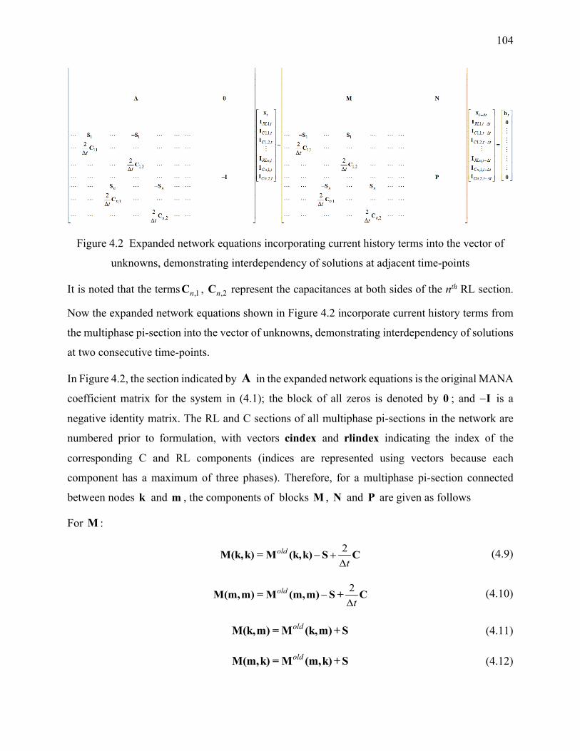
104

Figure 4.2 Expanded network equations incorporating current history terms into the vector of

unknowns, demonstrating interdependency of solutions at adjacent time-points

It is noted that the terms ,1nC , ,2nC represent the capacitances at both sides of the nth RL section.

Now the expanded network equations shown in Figure 4.2 incorporate current history terms from

the multiphase pi-section into the vector of unknowns, demonstrating interdependency of solutions

at two consecutive time-points.

In Figure 4.2, the section indicated by A in the expanded network equations is the original MANA

coefficient matrix for the system in (4.1); the block of all zeros is denoted by 0 ; and −I is a

negative identity matrix. The RL and C sections of all multiphase pi-sections in the network are

numbered prior to formulation, with vectors cindex and rlindex indicating the index of the

corresponding C and RL components (indices are represented using vectors because each

component has a maximum of three phases). Therefore, for a multiphase pi-section connected

between nodes k and m , the components of blocks M , N and P are given as follows

For M :

2old

t− +

∆M(k,k) = M (k,k) S C (4.9)

2old

t−

∆M(m,m) = M (m,m) S + C (4.10)

oldM(k,m) = M (k,m) + S (4.11)

oldM(m,k) = M (m,k) + S (4.12)

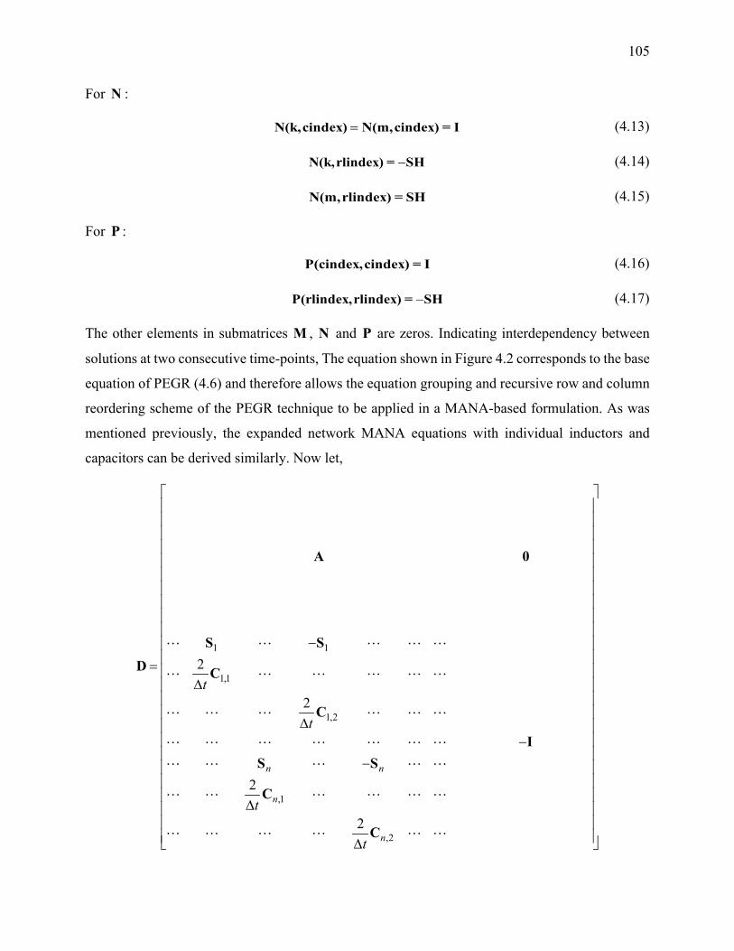
105

For N :

=N(k,cindex) N(m,cindex) = I (4.13)

−N(k,rlindex) = SH (4.14)

N(m,rlindex) = SH (4.15)

For P :

P(cindex,cindex) = I (4.16)

−P(rlindex,rlindex) = SH (4.17)

The other elements in submatrices M , N and P are zeros. Indicating interdependency between

solutions at two consecutive time-points, The equation shown in Figure 4.2 corresponds to the base

equation of PEGR (4.6) and therefore allows the equation grouping and recursive row and column

reordering scheme of the PEGR technique to be applied in a MANA-based formulation. As was

mentioned previously, the expanded network MANA equations with individual inductors and

capacitors can be derived similarly. Now let,

1 1

1,1

1,2

,1

,2

2

2

2

2

n n

n

n

t

t

t

t

− =

∆

∆ − −

∆ ∆

A 0

S SD C

C

IS S

C

C

106

1 1

1,1

1,2

,1

,2

2

2

2

2

n n

n

n

t

t

t

t

− =

∆

∆ −

∆ ∆

M N

S SO C

C

PS S

C

C

1,

1,1,

1,2,

,

,1,

,2,

t

RL t

C t

C tt

RLn t

Cn t

Cn t

=

xIII

x

III

t

t

b0

b =

0

The equation in Figure 4.2 can be rewritten in a more compact form,

107

t t t t−∆− =Dx Ox b (4.18)

In the expanded network equations (4.18), vectors tx and tb denote the expanded unknown and

right-hand-side vectors respectively. It is worth nothing that vector tb is now devoid of history

terms.

4.1.3 Grouping and recursive row and column reordering of expanded network

MANA equations

The original proposition of the PEGR technique restricts the total number of solution steps T of a

simulation to be 2T τ= (τ is an integer) in order that the simulation can be solved in 2log T steps

using / 2T processors [30]. This is unrealistic in practice in that a simulation can require any

number of solution steps and / 2T processors are usually unavailable to the user if the simulation

takes too many solution steps (T is an extremely large number). Hence, instead of grouping the

solutions at all T time-steps to construct a huge matrix as in the original PEGR proposition [30],

this section presents the implementation of the equation grouping and recursive row and column

reordering scheme used in the original PEGR technique in the new MANA-based parallel-in-time

approach with an example showing the grouping of network equations of 16 ( 416 2= ) time-steps,

thus solving the network for every 16 time-steps. It is noted that the algorithm can also

accommodate the solution of every 32, 64, 128, …, T time-steps ( 2T τ= , τ is an integer),

depending on the number of parallel processors available to the user. It is also worth mentioning

that the treatment of arbitrary topological changes and numbers of solution time-steps will be

presented in a later section.

Given equation (4.18), we can define,

1 2 16ˆ [ , ,..., ]=x x x x

1 2 16ˆ ˆ ˆ ˆ[ , ,..., ]=b b b b

Clearly, vectors x and b contain the solutions and the right-hand-side values of the first 16 time-

steps. A set of 16 vector equations of (4.18) can thus be written as,

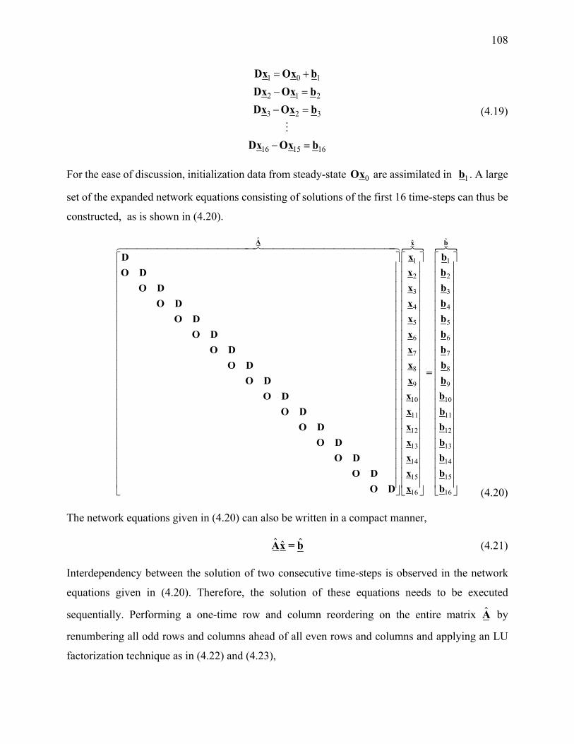
108

1 0 1

2 1 2

3 2 3

16 15 16

= +

− =− =

− =

Dx Ox bDx Ox bDx Ox b

Dx Ox b

(4.19)

For the ease of discussion, initialization data from steady-state 0Ox are assimilated in 1b . A large

set of the expanded network equations consisting of solutions of the first 16 time-steps can thus be

constructed, as is shown in (4.20).

ˆ

1

2

3

4

5

6

7

8

9

10

11

12

13

14

15

16

A

xDxO DxO DxO DxO DxO DxO DxO DxO DxO DxO DxO DxO DxO DxO DxO D

ˆˆ

1

2

3

4

5

6

7

8

9

10

11

12

13

14

15

16

bx

bbbbbbbb

=bbbbbbbb (4.20)

The network equations given in (4.20) can also be written in a compact manner,

ˆ ˆˆAx = b (4.21)

Interdependency between the solution of two consecutive time-steps is observed in the network

equations given in (4.20). Therefore, the solution of these equations needs to be executed

sequentially. Performing a one-time row and column reordering on the entire matrix A by

renumbering all odd rows and columns ahead of all even rows and columns and applying an LU

factorization technique as in (4.22) and (4.23),

109

[ ]

ˆ

ˆ ˆˆ ˆ ˆ ˆy

Αx = LUx = L Ux = Ly = b (4.22)

ˆ ˆ=Ux y (4.23)

the lower triangular equations in the L side for forward substitution to solve for y thus are,

L 1

3

5

7

9

11

13

15

2

4

6

8

10

12

14

16

yd y

d yd y

dy

dydydyd

o d yo f d y

o f d yo f d y

o f dy

o f dyo f dyo f dy

1

3

5

7

9

11

13

15

2

4

6

8

10

12

14

16

bbbbbbbb

=bbbbbbbb (4.24)

In (4.24), d , o and f represent diagonal, off-diagonal and fill-in blocks respectively. The vectors

1 3 16y , y , ...y and [ ]1 3 16b ,b , ...,b are vectors y and b after the one-time row and column

reordering. It is noted that d and o differ from D and O in equations (4.20) in that the former two

are the diagonal and off-diagonal elements after LU factorization, and the numerical values of each

d , o and f block are not necessarily identical. A remarkable fact is that this one-time row and

column reordering process results in fill-ins (represented by f blocks) where there was previously

none in equations (4.20). Nevertheless, the overall computational effort will be lower thanks to

parallelism, as will be seen hereinafter.

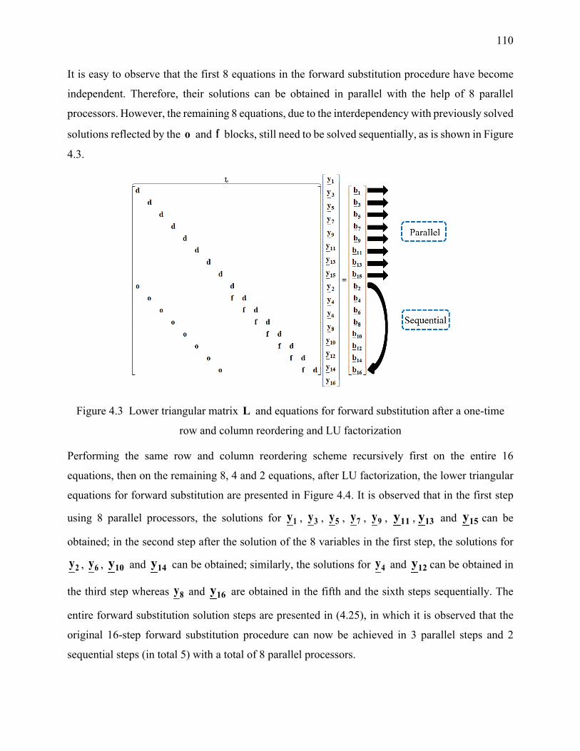
110

It is easy to observe that the first 8 equations in the forward substitution procedure have become

independent. Therefore, their solutions can be obtained in parallel with the help of 8 parallel

processors. However, the remaining 8 equations, due to the interdependency with previously solved

solutions reflected by the o and f blocks, still need to be solved sequentially, as is shown in Figure

4.3.

Figure 4.3 Lower triangular matrix L and equations for forward substitution after a one-time

row and column reordering and LU factorization

Performing the same row and column reordering scheme recursively first on the entire 16

equations, then on the remaining 8, 4 and 2 equations, after LU factorization, the lower triangular

equations for forward substitution are presented in Figure 4.4. It is observed that in the first step

using 8 parallel processors, the solutions for 1y , 3y , 5y , 7y , 9y , 11y , 13y and 15y can be

obtained; in the second step after the solution of the 8 variables in the first step, the solutions for

2y , 6y , 10y and 14y can be obtained; similarly, the solutions for 4y and 12y can be obtained in

the third step whereas 8y and 16y are obtained in the fifth and the sixth steps sequentially. The

entire forward substitution solution steps are presented in (4.25), in which it is observed that the

original 16-step forward substitution procedure can now be achieved in 3 parallel steps and 2

sequential steps (in total 5) with a total of 8 parallel processors.

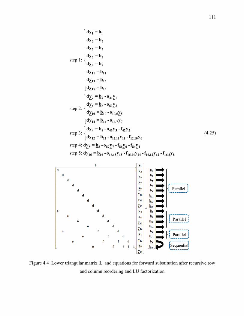
111

step 1:

step 2:

step 3:

1 1

3 3

5 5

7 7

9 9

11 11

13 13

15 15

2 2 21 1

6 6 63 3

10 10 10,5 5

14 14 14,7 7

4 4 43 3 42 2

12 12 12,11 11 12,10

dy = b

dy = b

dy = b

dy = b

dy = b

dy = b

dy = b

dy = b

dy = b - o y

dy = b - o y

dy = b - o y

dy = b - o y

dy = b - o y - f y

dy = b - o y - f y

step 4:

step 5:

6

8 8 87 7 86 6 84 4

16 16 16,15 15 16,14 14 16,12 12 16,8 8

dy = b - o y - f y - f y

dy = b - o y - f y - f y - f y

(4.25)

Figure 4.4 Lower triangular matrix L and equations for forward substitution after recursive row

and column reordering and LU factorization

112

Similarly, the upper triangular U matrix and equations for backward substitution are shown in

(4.26), where I , o and f represent identity, off-diagonal and fill-in blocks respectively. The entire

backward substitution steps are presented in (4.27). Therefore, the original 16-step backward

substitution procedure can be achieved in 4 steps, using 8 parallel processors.

In summary, using the original step-by-step methodology, the total number of steps in the forward

and backward substitutions is 32 for the solutions of 16 time-steps. However, applying the equation

grouping and recursive row and column reordering scheme, the total number of steps in the forward

and backward substitutions is reduced to 9 (5 steps in the forward substitution and 4 steps in the

backward substitution). Without topological changes in the network or iterations, the L and U

matrices remain unchanged. Therefore, major computation time gains can be expected in a time-

domain simulation scenario by grouping the MANA-based expanded network equations of every

16 time-steps together, as in (4.20), and solving them with the help of the recursive row and column

reordering scheme.

The equation grouping and recursive row and column reordering scheme can be applied on the

solutions of every 32, 64, 128, … time-steps in the exact same fashion. Higher computation time

gains are expected. Once again, the number of solutions to be grouped depends on the available

parallel processors in order to achieve maximal efficiency brought by the equation grouping and

recursive row and column reordering scheme (8, 16, 32, … processors are needed to group the

solutions of 16, 32, 64, …time-steps).

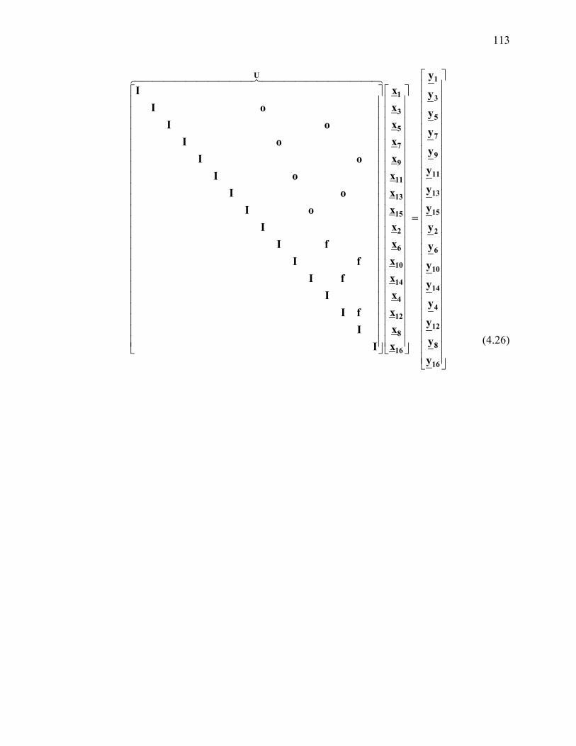
113

U 1

1 3

35

57

7

9

11

13

15

2

6

10

14

4

12

8

16

yxI yxI o yxI o yxI o

yxI oxI oxI oxI o

=xIxI fxI fxI fxIxI fxIxI

9

11

13

15

2

6

10

14

4

12

8

16

y

y

y

y

y

y

y

y

y

y

y

(4.26)

114

step 1:

step 2:

step 3:

16 16

8 8

4 4

2 2

1 1

12 12 12,8 8

10 10 10,8 8

6 6 64 4

3 3 32 2

9 9 9,8 8

5 5 54 4

3 3 32 2

14 14 14,12 12

13 13 1

Ix = y

Ix = y

Ix = y

Ix = y

Ix = y

Ix = y - f x

Ix = y - f x

Ix = y - f x

Ix = y - f x

Ix = y - f x

Ix = y - f x

Ix = y - f x

Ix = y - f x

Ix = y - f

step 4:

3,12 12

11 11 11,10 10

7 7 76 6

15 15 15,14 14

x

Ix = y - f x

Ix = y - f x

Ix = y - f x

(4.27)

4.2 Implementation of the PEGR-based parallel-in-time approach

This section tackles issues encountered in the implementation of the PEGR-based parallel-in-time

approach. It first elucidates the platform of implementation, which is C++ using API OpenMP

Multithreading. Then it proceeds to elaborate on measures taken to minimize false sharing, data

race as well as inconsistency between temporary view and memory in a parallel computing

environment. An important procedure in this parallel-in-time approach is the extraction of off-

diagonal block elements from the L and U factors after factorization for forward and backward

substitution, whose details are presented. Last but not least, since a discontinuity caused by

switching or any other topological change in the network can happen at an arbitrary time-point and

a time-domain simulation can consist of any number of simulation points whereas the PEGR-based

parallel-in-time approach solves the network equations for every 16, 32, 64, 128, … time-steps, the

treatment of arbitrary points of topological changes and numbers of simulation points is discussed.

115

4.2.1 Parallelization using OpenMP

It is noted the PEGR-based parallel-in-time approach proposed in this thesis is formulated using

sparse matrix techniques [97], which indicates that all the formulated matrices are represented as

sparse matrices, and all algorithms used in matrix manipulations cater to sparse matrices.

Furthermore, the KLU sparse linear solver [11]-[13] is adopted as the sparse matrix solver. The

entire algorithm is programmed in C++ language using API OpenMP Multithreading [98] for

parallelization during the forward and backward substitution processes. A snippet of the

parallelization process is shown as follows:

omp_set_dynamic(0); start = std::chrono::system_clock::now(); // parallelization for (int itr = 0; itr < tot_time_points / 64; itr++) { #pragma omp parallel num_threads(32) { #pragma omp sections { ////////////////////// thread 1 #pragma omp section { if (itr > 0) { sp_solve_thread0.init_first_element(sp_matL, b, itr); } sp_solve_thread0.solve_for_z(b, z_for_x, itr, 0); sp_solve_thread0.mat_vec_mult_subt_for_z(L1_p, L1_i, L1_x, b, z_for_x, itr, 0, 32 * size_sub_mat); sp_solve_thread0.solve_for_z(b, x, itr, 32 * size_sub_mat); sp_solve_thread0.mat_vec_mult_subt_for_z(L2_p, L2_i, L2_x, b, z_for_x, itr, 32 * size_sub_mat, 48 * size_sub_mat); sp_solve_thread0.solve_for_z(b, z_for_x, itr, 48 * size_sub_mat); sp_solve_thread0.mat_vec_mult_subt_for_z(L3_p, L3_i, L3_x, b, z_for_x, itr, 48 * size_sub_mat, 56 * size_sub_mat); sp_solve_thread0.solve_for_z(b, z_for_x, itr, 56 * size_sub_mat); sp_solve_thread0.mat_vec_mult_subt_for_z(L4_p, L4_i, L4_x, b, z_for_x, itr, 56 * size_sub_mat, 60 * size_sub_mat); sp_solve_thread0.solve_for_z(b, z_for_x, itr, 60 * size_sub_mat); sp_solve_thread0.mat_vec_mult_subt_for_z(L5_p, L5_i, L5_x, b, z_for_x, itr, 60 * size_sub_mat, 62 * size_sub_mat); sp_solve_thread0.solve_for_z(b, z_for_x, itr, 62 * size_sub_mat); sp_solve_thread0.mat_vec_mult_subt_for_z(L6_p, L6_i, L6_x, b, z_for_x, itr, 62 * size_sub_mat, 63 * size_sub_mat); sp_solve_thread0.solve_for_z(b, z_for_x, itr, 63 * size_sub_mat);

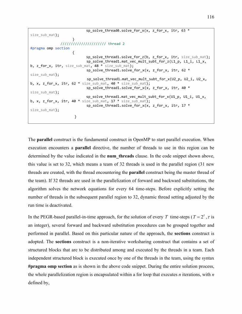
116

sp_solve_thread0.solve_for_x(x, z_for_x, itr, 63 * size_sub_mat); } ////////////////////// thread 2 #pragma omp section { sp_solve_thread1.solve_for_z(b, z_for_x, itr, size_sub_mat); sp_solve_thread1.mat_vec_mult_subt_for_z(L1_p, L1_i, L1_x, b, z_for_x, itr, size_sub_mat, 48 * size_sub_mat); sp_solve_thread1.solve_for_x(x, z_for_x, itr, 62 * size_sub_mat); sp_solve_thread1.mat_vec_mult_subt_for_x(U2_p, U2_i, U2_x, b, x, z_for_x, itr, 62 * size_sub_mat, 40 * size_sub_mat); sp_solve_thread1.solve_for_x(x, z_for_x, itr, 40 * size_sub_mat); sp_solve_thread1.mat_vec_mult_subt_for_x(U1_p, U1_i, U1_x, b, x, z_for_x, itr, 40 * size_sub_mat, 17 * size_sub_mat); sp_solve_thread1.solve_for_x(x, z_for_x, itr, 17 * size_sub_mat);

}

The parallel construct is the fundamental construct in OpenMP to start parallel execution. When

execution encounters a parallel directive, the number of threads to use in this region can be

determined by the value indicated in the num_threads clause. In the code snippet shown above,

this value is set to 32, which means a team of 32 threads is used in the parallel region (31 new

threads are created, with the thread encountering the parallel construct being the master thread of

the team). If 32 threads are used in the parallelization of forward and backward substitutions, the

algorithm solves the network equations for every 64 time-steps. Before explicitly setting the

number of threads in the subsequent parallel region to 32, dynamic thread setting adjusted by the

run time is deactivated.

In the PEGR-based parallel-in-time approach, for the solution of every T time-steps ( 2T τ= ,τ is

an integer), several forward and backward substitution procedures can be grouped together and

performed in parallel. Based on this particular nature of the approach, the sections construct is

adopted. The sections construct is a non-iterative worksharing construct that contains a set of

structured blocks that are to be distributed among and executed by the threads in a team. Each

independent structured block is executed once by one of the threads in the team, using the syntax

#pragma omp section as is shown in the above code snippet. During the entire solution process,

the whole parallelization region is encapsulated within a for loop that executes n iterations, with n

defined by,

117

Total number of time-stepsnT

= (4.41)

where T is the number of time-steps the algorithm solves in a single iteration using a total number

of / 2T threads. It is to be modified depending on the actual number of threads used in the

algorithm. Moreover, the discussion here solely aims to shed light on the realization of

parallelization in the algorithm for the PEGR-based parallel-in-time approach without considering

discontinuity or topological changes in the network. More details on the constructs and clauses

used in the algorithm, as presented in the code snippet, can be found in [98] and [99].

4.2.2 Measures against false sharing, data race and inconsistency between

temporary view and memory

4.2.2.1 Minimizing false sharing

False sharing occurs when processors in a shared-memory parallel system make references to

different data objects within the same coherence block (cache line or page), thereby inducing

“unnecessary” coherence operations. Specifically, a thread attempts to periodically access data that

is not altered by another party but share the same cache block with data that are altered. The caching

protocol therefore forces the thread to reload the whole unit despite a lack of logical necessity. It

is widely believed to be a performance-degrading usage pattern for parallel programs [100]. Several

techniques are employed in this algorithm in order to minimize false sharing. The goal is to ensure

that variables causing false sharing are spaced far enough apart in memory that they cannot reside

on the same cache line.

• __declspec (align(n))

This directive can force alignment of individual variables on the cache line boundaries. In modern-

day CPUs, the size of the cache line is usually 64 bytes. Therefore, the alignment value is set to 64,

as is shown in the following code snippet:

_declspec(align(64)) int tot_time_points = 8192; _declspec(align(64)) int size_sub_mat = 50; _declspec(align(64)) double dt = 0.00005;

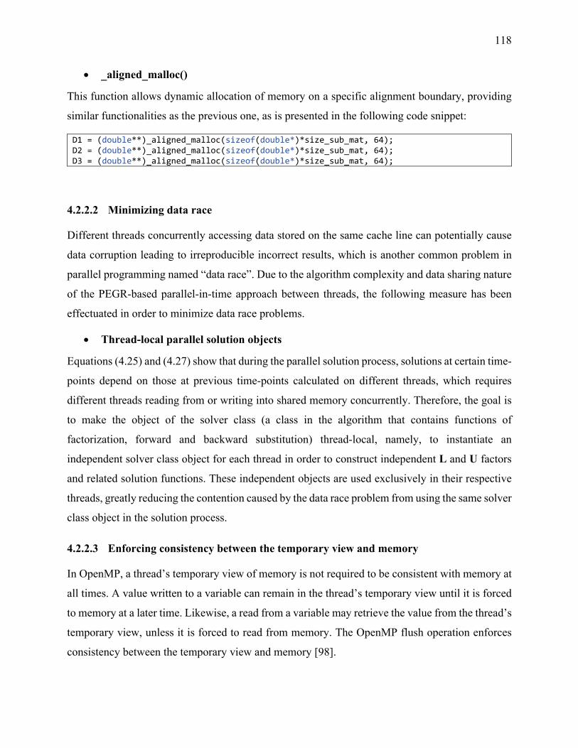
118

• _aligned_malloc()

This function allows dynamic allocation of memory on a specific alignment boundary, providing

similar functionalities as the previous one, as is presented in the following code snippet:

D1 = (double**)_aligned_malloc(sizeof(double*)*size_sub_mat, 64); D2 = (double**)_aligned_malloc(sizeof(double*)*size_sub_mat, 64); D3 = (double**)_aligned_malloc(sizeof(double*)*size_sub_mat, 64);

4.2.2.2 Minimizing data race

Different threads concurrently accessing data stored on the same cache line can potentially cause

data corruption leading to irreproducible incorrect results, which is another common problem in

parallel programming named “data race”. Due to the algorithm complexity and data sharing nature

of the PEGR-based parallel-in-time approach between threads, the following measure has been

effectuated in order to minimize data race problems.

• Thread-local parallel solution objects

Equations (4.25) and (4.27) show that during the parallel solution process, solutions at certain time-

points depend on those at previous time-points calculated on different threads, which requires

different threads reading from or writing into shared memory concurrently. Therefore, the goal is

to make the object of the solver class (a class in the algorithm that contains functions of

factorization, forward and backward substitution) thread-local, namely, to instantiate an

independent solver class object for each thread in order to construct independent L and U factors

and related solution functions. These independent objects are used exclusively in their respective

threads, greatly reducing the contention caused by the data race problem from using the same solver

class object in the solution process.

4.2.2.3 Enforcing consistency between the temporary view and memory

In OpenMP, a thread’s temporary view of memory is not required to be consistent with memory at

all times. A value written to a variable can remain in the thread’s temporary view until it is forced

to memory at a later time. Likewise, a read from a variable may retrieve the value from the thread’s

temporary view, unless it is forced to read from memory. The OpenMP flush operation enforces

consistency between the temporary view and memory [98].

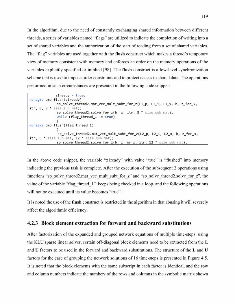
119

In the algorithm, due to the need of constantly exchanging shared information between different

threads, a series of variables named “flags” are utilized to indicate the completion of writing into a

set of shared variables and the authorization of the start of reading from a set of shared variables.

The “flag” variables are used together with the flush construct which makes a thread’s temporary

view of memory consistent with memory and enforces an order on the memory operations of the

variables explicitly specified or implied [98]. The flush construct is a low-level synchronization

scheme that is used to impose order constraints and to protect access to shared data. The operations

performed in such circumstances are presented in the following code snippet:

z1ready = true; #pragma omp flush(z1ready) sp_solve_thread2.mat_vec_mult_subt_for_z(L1_p, L1_i, L1_x, b, z_for_x, itr, 0, 8 * size_sub_mat); sp_solve_thread2.solve_for_z(b, x, itr, 8 * size_sub_mat); while (flag_thread_1 != true) { #pragma omp flush(flag_thread_1) } sp_solve_thread2.mat_vec_mult_subt_for_z(L2_p, L2_i, L2_x, b, z_for_x, itr, 8 * size_sub_mat, 12 * size_sub_mat); sp_solve_thread2.solve_for_z(b, z_for_x, itr, 12 * size_sub_mat);

In the above code snippet, the variable “z1ready” with value “true” is “flushed” into memory

indicating the previous task is complete. After the execution of the subsequent 2 operations using

functions “sp_solve_thread2.mat_vec_mult_subt_for_z” and “sp_solve_thread2.solve_for_z”, the

value of the variable “flag_thread_1” keeps being checked in a loop, and the following operations

will not be executed until its value becomes “true”.

It is noted the use of the flush construct is restricted in the algorithm in that abusing it will severely

affect the algorithmic efficiency.

4.2.3 Block element extraction for forward and backward substitutions

After factorization of the expanded and grouped network equations of multiple time-steps using

the KLU sparse linear solver, certain off-diagonal block elements need to be extracted from the L

and U factors to be used in the forward and backward substitutions. The structure of the L and U

factors for the case of grouping the network solutions of 16 time-steps is presented in Figure 4.5.

It is noted that the block elements with the same subscript in each factor is identical, and the row

and column numbers indicate the numbers of the rows and columns in the symbolic matrix shown

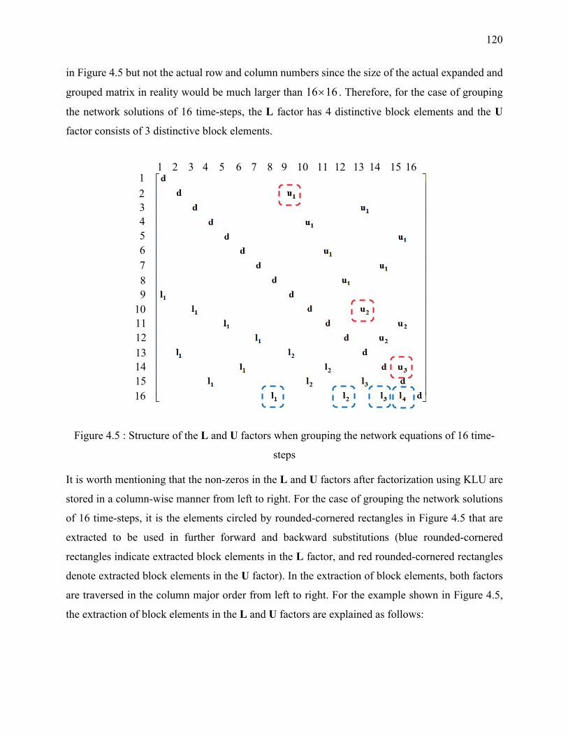
120

in Figure 4.5 but not the actual row and column numbers since the size of the actual expanded and

grouped matrix in reality would be much larger than 16 16× . Therefore, for the case of grouping

the network solutions of 16 time-steps, the L factor has 4 distinctive block elements and the U

factor consists of 3 distinctive block elements.

Figure 4.5 : Structure of the L and U factors when grouping the network equations of 16 time-

steps

It is worth mentioning that the non-zeros in the L and U factors after factorization using KLU are

stored in a column-wise manner from left to right. For the case of grouping the network solutions

of 16 time-steps, it is the elements circled by rounded-cornered rectangles in Figure 4.5 that are

extracted to be used in further forward and backward substitutions (blue rounded-cornered

rectangles indicate extracted block elements in the L factor, and red rounded-cornered rectangles

denote extracted block elements in the U factor). In the extraction of block elements, both factors

are traversed in the column major order from left to right. For the example shown in Figure 4.5,

the extraction of block elements in the L and U factors are explained as follows:

1 2 3 4 5 6 7 8 9 10 11 12 13 14 15 16 1 2 3 4 5 6 7 8 9

10 11 12 13 14 15 16

121

For the extraction of block elements in the L factor:

1) When the traverse hits symbolic row 16, extraction of 1l starts

2) When the traverse hits symbolic row 9 (the diagonal block element in the next symbolic

column), mark the completion of 1l extraction

3) When the traverse hits symbolic row 16 and 1l extraction is completed, extraction of 2l

starts



5) When the traverse hits symbolic row 16 and 2l extraction is completed, extraction of 3l

starts



7) When the traverse hits symbolic row 15, 3l extraction is completed and the traverse

element count 1L diagi nz nz≤ − − , extraction of 4l starts

For the extraction of block elements in the U factor:

1) When the traverse hits symbolic row 8 (the diagonal element in the 8th symbolic row),

mark the extraction of 1u ready (it is the first block element in the next symbolic column)

2) When the traverse hits symbolic row 2 and the extraction of 1u is ready, extraction of

1u starts

3) When the traverse hits symbolic row 4 (the first block element in the next symbolic

column), mark the completion of 1u extraction

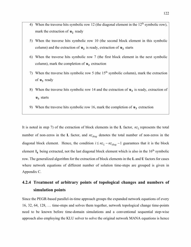
122

4) When the traverse hits symbolic row 12 (the diagonal element in the 12th symbolic row),

mark the extraction of 2u ready

5) When the traverse hits symbolic row 10 (the second block element in this symbolic

column) and the extraction of 2u is ready, extraction of 2u starts

6) When the traverse hits symbolic row 7 (the first block element in the next symbolic

column), mark the completion of 2u extraction

7) When the traverse hits symbolic row 5 (the 15th symbolic column), mark the extraction

of 3u ready

8) When the traverse hits symbolic row 14 and the extraction of 3u is ready, extraction of

3u starts

9) When the traverse hits symbolic row 16, mark the completion of 3u extraction

It is noted in step 7) of the extraction of block elements in the L factor, Lnz represents the total

number of non-zeros in the L factor, and diagnz denotes the total number of non-zeros in the

diagonal block element. Hence, the condition 1L diagi nz nz≤ − − guarantees that it is the block

element 4l being extracted, not the last diagonal block element which is also in the 16th symbolic

row. The generalized algorithm for the extraction of block elements in the L and U factors for cases

where network equations of different number of solution time-steps are grouped is given in

Appendix C.

4.2.4 Treatment of arbitrary points of topological changes and numbers of

simulation points

Since the PEGR-based parallel-in-time approach groups the expanded network equations of every

16, 32, 64, 128, … time-steps and solves them together, network topological change time-points

need to be known before time-domain simulations and a conventional sequential step-wise

approach also employing the KLU solver to solve the original network MANA equations is hence

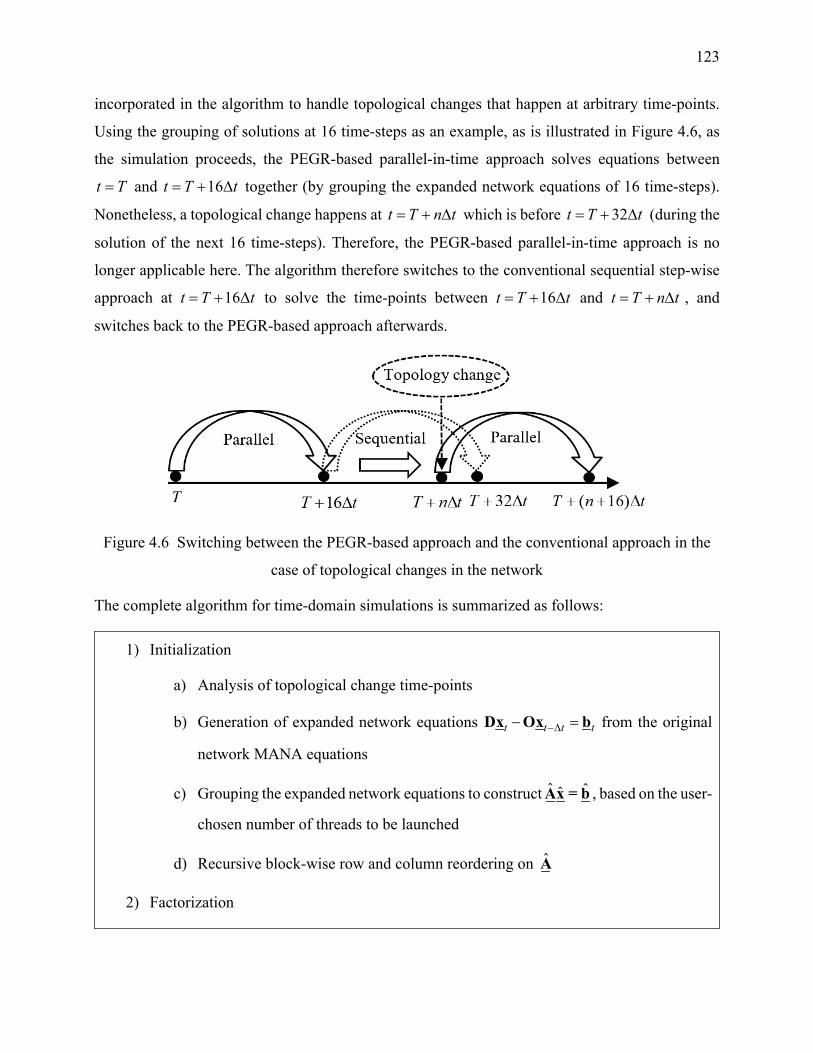
123

incorporated in the algorithm to handle topological changes that happen at arbitrary time-points.

Using the grouping of solutions at 16 time-steps as an example, as is illustrated in Figure 4.6, as

the simulation proceeds, the PEGR-based parallel-in-time approach solves equations between

t T= and 16t T t= + ∆ together (by grouping the expanded network equations of 16 time-steps).

Nonetheless, a topological change happens at t T n t= + ∆ which is before 32t T t= + ∆ (during the

solution of the next 16 time-steps). Therefore, the PEGR-based parallel-in-time approach is no

longer applicable here. The algorithm therefore switches to the conventional sequential step-wise

approach at 16t T t= + ∆ to solve the time-points between 16t T t= + ∆ and t T n t= + ∆ , and

switches back to the PEGR-based approach afterwards.

Figure 4.6 Switching between the PEGR-based approach and the conventional approach in the

case of topological changes in the network

The complete algorithm for time-domain simulations is summarized as follows:

1) Initialization

a) Analysis of topological change time-points

b) Generation of expanded network equations t t t t−∆− =Dx Ox b from the original

network MANA equations

c) Grouping the expanded network equations to construct ˆ ˆˆAx = b , based on the user-

chosen number of threads to be launched

d) Recursive block-wise row and column reordering on A

2) Factorization

124

a) Symbolic and numeric factorization of the reordered matrix A using KLU

b) L and U factor block element extraction from the results of numeric factorization

for the use in forward and backward substitutions in the PEGR-based parallel-in-

time approach

c) Symbolic and numeric factorization of the original network MANA coefficient

matrix using KLU

3) Solution

a) Solution using the PEGR-based parallel-in-time approach for every n time-steps

(n is twice the user-chosen number of launched threads)

b) Sequential step-wise solution based on the conventional approach before reaching

points of topological changes or end of simulation

c) If it is the end of the simulation, go to step 4); if not, modify and update the D

and O blocks in the reordered matrix as well as the original network MANA

coefficient matrix, then go back to step 2)

4) End of time-domain simulation

4.3 Conclusion

This chapter presented the development of a new parallel-in-time approach implementing the

parallel-in-time equation grouping and reordering (PEGR) scheme for power system EMT

simulations. It first discussed the adaption of the PEGR technique originally formulated in state-

space to the modified-augmented-nodal analysis (MANA) through the expansion of the original

network equations and explicitly manifesting interdependency between consecutive solution time-

steps. It then demonstrated the PEGR technique used in the new parallel-in-time approach as well

as the original state-space proposition through an example in which the solutions of 16 time-steps

are grouped. Subsequently, detailed programming issues encountered in the implementation of the

PEGR-based parallel-in-time approach in C++ were discussed, which include the OpenMP

platform for parallelization, particular measures and programming considerations to minimize false

sharing, data race as well as maintaining consistency between the temporary view and memory in

125

OpenMP, block elements extraction from the L and U factors after factorization to be used in the

forward and backward substitutions, and the treatment of arbitrary points of topological changes

and numbers of simulation points.

126

CHAPTER 5 TEST CASES AND SIMULATION RESULTS OF THE

PEGR-BASED PARALLEL-IN-TIME APPROACH

This chapter presents simulation results of the PEGR-based parallel-in-time approach developed

in this thesis. As in the FMI-based co-simulation approach proposed in early chapters of this thesis,

the tests on the PEGR-based parallel-in-time approach aim to validate this approach for accuracy

control and solution speedup in power system time-domain simulations. New power system

simulation benchmarks are used for the validation of each aspect. The validation of accuracy is

based on the comparison of various waveforms using the PEGR-based parallel-in-time approach

with those obtained from an EMT-type solver [2], and solution speedup is validated by comparing

solution times using the proposed approach to those using the conventional step-wise solution

scheme. The advantages of the proposed PEGR-based parallel-in-time approach for large-scale

power system time-domain simulations are demonstrated, and a discussion on the obtained results

is presented. All tests are executed on the PC with 24 cores and 48 logical processors whose

hardware and software configurations are given in Table 3.18. In all test cases, a simulation interval

of 3 s is chosen, and a phase-a-to-ground fault scenario occurring at 2t s= and cleared at 2.1t s=

is simulated in time-domain.

5.1 Accuracy validation

In this section, the accuracy of the PEGR-based parallel-in-time approach proposed in this thesis

is validated by examining voltages on various buses and the fault current during a fault scenario.

The reference waveforms are those found from an EMT-type solver [2] with ultimate accuracy.

The Network-5 benchmark, as is shown in Figure 5.1, is used in the test, with the fault location

clearly indicated. It is based on the original IEEE-34 bus test system [101], [102]. In this

benchmark, the generator is represented by a three-phase voltage source (AC at bus 800); the

transformers and regulators (T832_888, TAP852_832 and TAP814_850) are modelled by three-

phase two coupled windings; all the transmission lines are modelled by coupled pi-sections; and

the loads (both spot loads and distributed loads) are represented by three-phase resistors, inductors

and capacitors. Therefore, the network illustrated in Figure 5.1 is completely linear.

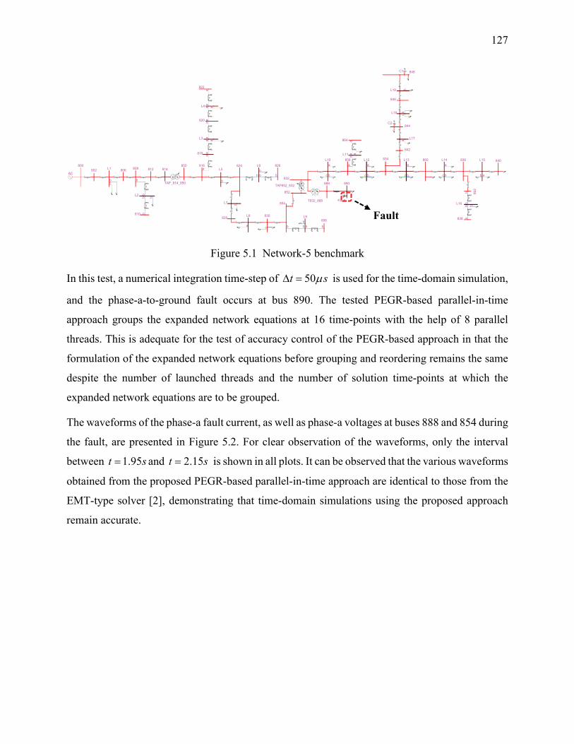
127


In this test, a numerical integration time-step of 50t sµ∆ = is used for the time-domain simulation,

and the phase-a-to-ground fault occurs at bus 890. The tested PEGR-based parallel-in-time

approach groups the expanded network equations at 16 time-points with the help of 8 parallel

threads. This is adequate for the test of accuracy control of the PEGR-based approach in that the

formulation of the expanded network equations before grouping and reordering remains the same

despite the number of launched threads and the number of solution time-points at which the

expanded network equations are to be grouped.

The waveforms of the phase-a fault current, as well as phase-a voltages at buses 888 and 854 during

the fault, are presented in Figure 5.2. For clear observation of the waveforms, only the interval

between 1.95t s= and 2.15t s= is shown in all plots. It can be observed that the various waveforms

obtained from the proposed PEGR-based parallel-in-time approach are identical to those from the

EMT-type solver [2], demonstrating that time-domain simulations using the proposed approach

remain accurate.

PI+

PI+

1 2

T832_888?

24.9/4.16

LF

PI

+R

L+

LF

PI+

PI+

PI+

RL

+

PI+

PI+

PI+

LF

LF

LF

LF

LF+

C2

LF

LF

PI+

RL

+

LF

LF

LF

LF

LF

LF

LF

RL

+

LF

LF

LF

PI+

LF+C1

PI

+

LF LF LF LF

LF

LF

F

Fault

RL+

PI+

PI+

PI+

PI+

PI+

PI+

PI+

PI+

PI+

PI+

PI+

PI+

PI+

LF LF

RL

+R

L+

LF

PI+

RL

+R

L+

RL

+

LF

PI+

RL+

LF

RL+

LF

RL

+R

L+

1 2

TAP_814_850

PI

+

LF

RL+LF

PI+

LFLF

PI+

PI+

PI+

PI

+

PI+

12TAP852_832

+

AC

LF

b

854

b bbL9

b 862

bbbL16

842

aaaL11

L12

c b

a

846

L13a

bc

L15

b a

bL19

858a

L10

c b

a

a864

834 860 L14

c

a

b

836

b838

bcL18

844

a L17

848

840

856

b

812 a816

b

808

cb

L1802 806

b810

bbbL2

aa818

aa

aL4

aa820

aaaL3

a

822

bbb

L6

b

L5

b

826824814

850

cL7

828

c

830

a

L8

832

852

890888

800

Fault

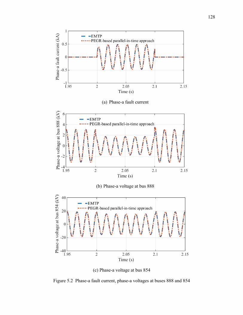
128

(a) Phase-a fault current

(b) Phase-a voltage at bus 888

(c) Phase-a voltage at bus 854

Figure 5.2 Phase-a fault current, phase-a voltages at buses 888 and 854

129

5.2 Computation time gains

The validation of computation time gains is based on the comparison of the solution times of the

benchmarks simulated with the PEGR-based parallel-in-time approach proposed in this thesis and

using the conventional sequential step-wise scheme. Its objective is to demonstrate the numerical

performance advantages of the proposed parallel-in-time approach on power system networks of

different levels of complexity. The 24-core PC, whose hardware and software configurations are

given in Table 3.18, is used in the tests of computation time gains.

It is worth noting that the purpose here is not to compare the performance of the PEGR-based

parallel-in-time approach developed in this thesis with that of any highly optimized commercial

power system simulation packages, but to demonstrate the numerical advantages of the new

methodology brought by grouping and recursive row and column reordering of expanded network

equations over the conventional sequential step-wise solution scheme. Hence, the solution times

obtained from the PEGR-based parallel-in-time approach are compared with a conventional

sequential step-wise solution scheme also implemented in C++ and employing the KLU sparse

linear solver as the matrix solver.

5.2.1 Test case 1

The first test case is based on the Network-5 benchmark shown in Figure 5.1. It is performed on

the original Network-5 benchmark which is a 34-bus network as well as on a 170-bus network

constructed by replicating the Network-5 benchmark in Figure 5.1 five times. Similarly, all

transmission lines in the 170-bus network are modelled by coupled pi-sections, and all loads are

modelled by three-phase resistors, inductors and capacitors. A simulation interval of 3 s is chosen,

with a numerical integration time-step of 50 µs. In all tests, a phase-a-to-ground fault occurring at

2t s= and cleared at 2.1t s= is simulated in time-domain. It is noted that different numbers of

threads 8, 16 and 32 are used in the tests with the PEGR-based parallel-in-time approach on the

24-core PC (Table 3.18), corresponding to the numbers of cores used 4, 8 and 16 respectively. The

expanded network equations are thus grouped for every 16, 32, and 64 time-steps. The performance

timings of both the conventional sequential step-wise approach and the PEGR-based parallel-in-

time approach are presented in Table 5.1, in which solution times refer to the time consumed in the

factorization of network equations and their solutions throughout the entire simulation interval in

130

time-domain for the conventional sequential step-wise approach, and to the time consumed in

initialization, factorization and solution, as shown in Section 4.2.4, for the PEGR-based parallel-

in-time approach. It is noted that the number of launched threads for the conventional step-wise

approach is marked as “N/A”, indicating that this approach does not involve parallelization.

Table 5.1 Performance timings of test case 1

Step-wise approach PEGR-based approach Number of launched threads N/A 8 16 32 34-bus network solution times (s) 83.72 50.43 39.03 28.20 170-bus network solution times (s) 444.53 233.16 170.45 125.53

Based on the data presented in Table 5.1, the solution time speedup using the PEGR-based

approach compared to the conventional sequential step-wise approach with respect to the number

of launched threads in the simulation can be calculated and is shown in Figure 5.3 for both test

networks.

Figure 5.3 Solution time speedup using the PEGR-based parallel-in-time approach with respect

to the number of launched threads in the simulation for test case 1

5.2.2 Test case 2

The second test case is based on the Network-6 benchmark shown in Figure 5.4. It is the EMT

version of the original IEEE-14 test system. The parameters for this benchmark can be found in

[103]. Similar to the first test case presented in the previous section, in this test, the generators are

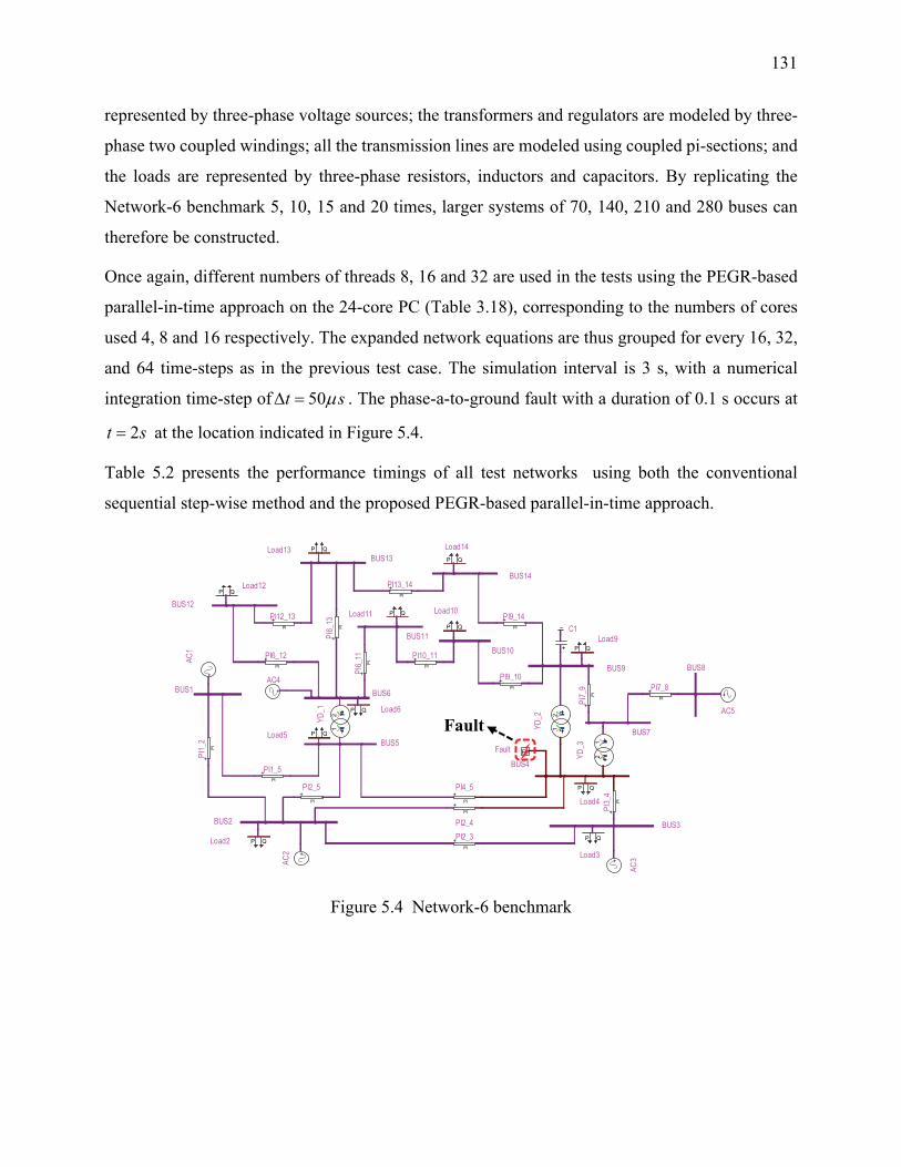
131

represented by three-phase voltage sources; the transformers and regulators are modeled by three-

phase two coupled windings; all the transmission lines are modeled using coupled pi-sections; and

the loads are represented by three-phase resistors, inductors and capacitors. By replicating the

Network-6 benchmark 5, 10, 15 and 20 times, larger systems of 70, 140, 210 and 280 buses can

therefore be constructed.

Once again, different numbers of threads 8, 16 and 32 are used in the tests using the PEGR-based

parallel-in-time approach on the 24-core PC (Table 3.18), corresponding to the numbers of cores

used 4, 8 and 16 respectively. The expanded network equations are thus grouped for every 16, 32,

and 64 time-steps as in the previous test case. The simulation interval is 3 s, with a numerical

integration time-step of 50t sµ∆ = . The phase-a-to-ground fault with a duration of 0.1 s occurs at

2t s= at the location indicated in Figure 5.4.

Table 5.2 presents the performance timings of all test networks using both the conventional

sequential step-wise method and the proposed PEGR-based parallel-in-time approach.


+

AC1

+

AC2

P QLoad2

+

AC4

+

AC5

+

AC3

P QLoad5

P Q

Load3

P Q

Load4

P Q Load6

P QLoad12

P QLoad13P Q

Load14

P Q

Load10

P QLoad9

P QLoad11

12YD

_1

12

YD_2

12YD

_3

+

C1

FFault

PI+PI13_14

PI+PI12_13

PI+PI6_12

PI+PI

1_2

PI+PI1_5

PI+PI2_5

PI+PI4_5

PI+

PI2_4

PI+PI2_3

PI+PI9_14

PI+PI10_11

PI+PI9_10

PI+PI7_8

PI+PI

6_13

PI+PI

6_11

PI+P

I7_9

PI+PI

3_4

BUS12

BUS7

BUS13

BUS14

BUS8BUS9

BUS5

BUS4

BUS1

BUS2

BUS11BUS10

BUS6

BUS3

Fault

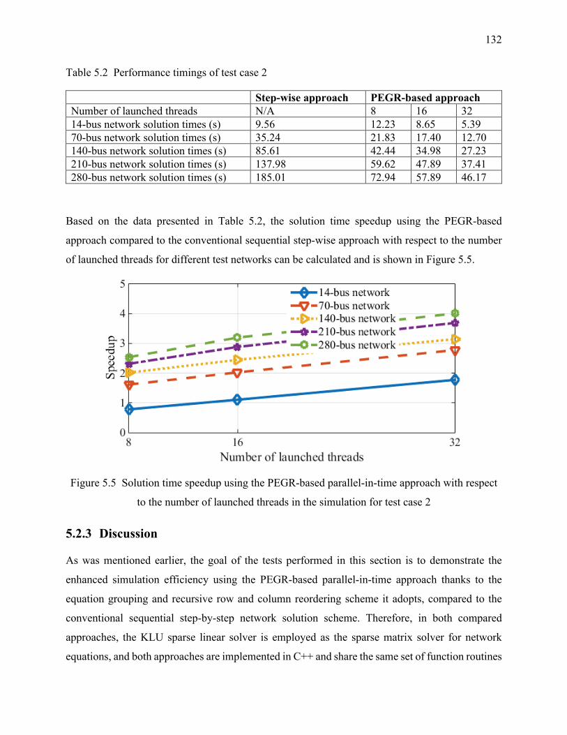
132

Table 5.2 Performance timings of test case 2

Step-wise approach PEGR-based approach Number of launched threads N/A 8 16 32 14-bus network solution times (s) 9.56 12.23 8.65 5.39 70-bus network solution times (s) 35.24 21.83 17.40 12.70 140-bus network solution times (s) 85.61 42.44 34.98 27.23 210-bus network solution times (s) 137.98 59.62 47.89 37.41 280-bus network solution times (s) 185.01 72.94 57.89 46.17

Based on the data presented in Table 5.2, the solution time speedup using the PEGR-based

approach compared to the conventional sequential step-wise approach with respect to the number

of launched threads for different test networks can be calculated and is shown in Figure 5.5.

Figure 5.5 Solution time speedup using the PEGR-based parallel-in-time approach with respect

to the number of launched threads in the simulation for test case 2

5.2.3 Discussion

As was mentioned earlier, the goal of the tests performed in this section is to demonstrate the

enhanced simulation efficiency using the PEGR-based parallel-in-time approach thanks to the

equation grouping and recursive row and column reordering scheme it adopts, compared to the

conventional sequential step-by-step network solution scheme. Therefore, in both compared

approaches, the KLU sparse linear solver is employed as the sparse matrix solver for network

equations, and both approaches are implemented in C++ and share the same set of function routines

133

in network matrix factorization, solution, forward and backward substitutions. This aims to create

a common platform to compare the two solution schemes which are the parallel-in-time solution

scheme and the conventional sequential step-wise solution scheme in order to demonstrate the

numerical advantages of the former, whereas not to compare any two specific solvers, . This is why

the performance timings using the PEGR-based parallel-in-time approach for both test cases

presented in Table 5.1 and Table 5.2 could still be inferior to commercialized power system

network solver with highly optimized routines [2] for the particular test cases presented here.

The performance timings presented in Table 5.1 and Table 5.2 include all necessary procedures in

time-domain simulations. Particularly for the case using the PEGR-based parallel-in-time

approach, it includes all three stages shown in Section 4.2.4, that is to say, the equation grouping

and recursive row and column reordering, factorization and refactorization of the grouped

expanded network equations whose size is much larger than that of the original network equations,

as well as extraction of block elements for forward and backward substitutions, are also included.

This proves, through the results presented in Figure 5.3 and Figure 5.5, that despite the need of

operating on a much larger sparse matrix comprised of solutions at 16, 32 and even 64 time-steps,

the proposed parallel-in-time approach can still be more efficient than the conventional sequential

step-wise solution scheme.

From Figure 5.3 and Figure 5.5, a few conclusions can be drawn:

• Higher gains in a simulation environment with more threads

This is fairly easy to understand from the original proposition of the PEGR scheme, as the recursive

row and column reordering scheme was designed such that the total solution steps needed to solve

a power system network can be theoretically logarithmically reduced [30]. Therefore, the more

threads the simulation launches, the more forward and backward substitution steps that can be

parallelized, which leads to an even more reduced number of total solution steps needed compared

to the conventional step-wise solution scheme.

Nonetheless, it is also observed that the actual computation time gains obtained in both test cases

are lower than those expected in the original proposition [30]. For instance, the original proposition

suggests that the total number of forward substitution steps will be reduced to 4, 5 and 6, as

compared to 16, 32 and 64, if 8, 16, and 32 parallel processors are available. However, firstly the

original proposition only refers to the numbers that forward substitution steps can be theoretically

134

reduced to with sufficient parallel processors whilst not considering other procedures needed in

time-domain simulations using the PEGR-based parallel-in-time approach such as equation

grouping, recursive row and column reordering of grouped network equations, factorization and

refactorization of the reordered and grouped network equations as well as block element extraction.

Secondly, certain measures adopted in the implementation of such an approach in C++ with

OpenMP Multithreading, such as enforcing consistency between the temporary view and memory

by using the flush construct, have negative impacts on the total solution times. Thirdly, overhead

caused by the inner mechanism of OpenMP also impacts the performance of the proposed PEGR-

based approach negatively.

• Higher gains on larger networks

It can be observed from Figure 5.3 and Figure 5.5 that for the same number of launched threads in

a simulation, as the network becomes larger, higher computation time gains can be achieved. This

is because for a given number of launched threads, the computational efficiency enhancement

brought by the PEGR-based approach for smaller networks is dwarfed by the time consumed in the

supplementary operations in the PEGR-based approach that are not necessary in the conventional

step-wise solution scheme, considering that the adopted sparse linear solver KLU is sufficiently

optimized thus highly efficient for the solution of smaller networks; however, as the network grows

larger, the time consumed in the supplementary operations in the PEGR-based approach becomes

less significant, the computational efficiency enhancement brought by the PEGR-based approach

therefore becomes more significant.

Despite the potential performance enhancement brought by the PEGR-based approach, there exist

certain limitations in the implementation of the PEGR-based approach on realistic large-scale

power system time-domain simulations:

• Higher formulation and solution complexity

Apart from formulating the original network MANA coefficient matrix, the PEGR-based approach

requires special treatment of the history terms in energy storage components such that

interdependency between network solutions at two consecutive time-points can be obtained.

Subsequently, the equation grouping and recursive row and column reordering procedures with

respect to the number of launched threads need to be performed in order to achieve solution

parallelism. After network matrix factorization, an extra block element extraction procedure is

135

required in the forward and backward substitution processes. All of the aboved-mentioned

procedures, which do not exist in the original MANA formulation method, add to the formulation

and solution complexity.

• More challenges on the PC memory capacity

The PEGR-approach requires operations on a huge network matrix consisting of solutions at

2T τ= (τ is an integer) time-steps, where T could be 16, 32, 64, 128, etc. Moreover, the inclusion

of history terms of energy storage components further increases the size of the network matrix for

the solution of a single time-step, compared to that of the original network MANA coefficient

matrix. Therefore, the implementation of the PEGR-based approach on large-scale networks would

pose great challenges on the PC memory capacity in terms of storage of certain vectors and matrices

used in the factorization and solution procedures.

• Knowledge of network topological change time-points prior to simulation start

Due to the nature of the PEGR-based approach of solving the network at every 16, 32, 64, …, T

time-steps ( 2T τ= ,τ is an integer), the network topological change time-points (fault, switching,

etc.) need to be known and analyzed prior to time-domain simulation start in order that a step-wise

conventional approach can be used to handle the topological changes. This is because the network

solution of every 16, 32, 64, …T time-steps ( 2T τ= ,τ is an integer) using the PEGR-approach is

a complete process and cannot be broken or stopped in the middle due to an arbitrary topological

change. This differs from the conventional EMT approach [2] and would introduce supplementary

burden into the pre-processing and solution procedures. Furthermore, although computation time

gains are observed in the test cases presented in this thesis, performance deterioration could happen

due to extensive switching between two types of solvers in test cases with multiple topological

changes.

• Difficulty in handling non-linearity

In the original PEGR technique, it was proposed to isolate nonlinear equations, group them and

solve them independently from linear equations using the Newton method [30]. The problems with

this proposition are: firstly, obtaining good initial estimates for a set of nonlinear equations

comprised of the solutions at multiple time-steps in order to lower the number of iterations and

achieve convergence is not straightforward; secondly, the interaction and data exchange between

136

linear and nonlinear equations in a realistic complex power system network are not answered for.

A numerical example of solving one single isolated nonlinear equation using the PEGR technique

was presented in [30], demonstrating the feasibility of the PEGR technique in handling non-

linearity, there is, however, not sufficient proof that the above-mentioned two problems could be

accounted for by this proposition. EMTP [2] linearizes nonlinear components by the method of

“piecewise linearization”, formulates both linear and nonlinear components into the MANA

coefficient matrix and performs iterations within the solution of each time-step to reach

convergence. Since the PEGR-based approach proposed in this thesis is based on the original

MANA formulation in EMTP [2], it would require that iterations be performed within the solution

of each time-step, which is impractical considering the PEGR-based approach solves the entire

network at multiple time-steps together as a complete procedure. Therefore, the PEGR-based

approach can only be implemented on linear networks if the MANA formulation method is kept as

a base method.

5.3 Conclusion

Test results using the PEGR-based parallel-in-time approach developed in this thesis were

presented in this chapter. The tests performed in this chapter aimed to validate the accuracy of the

approach and the computation time gains that can be achieved in power system time-domain

simulations. Two new benchmarks, as well as those constructed using their multiple replicas

representing power systems of different levels of complexities, were used in the tests. Accuracy of

the PEGR-based parallel-in-time approach was validated by comparing various waveforms using

the PEGR-based approach with those obtained from an EMT-type solver, whereas computation

time gains were demonstrated by comparing time-domain solution times using the developed

approach to those using the conventional step-wise solution scheme. The advantages of the

proposed PEGR-based parallel-in-time approach for large-scale power system time-domain

simulations were demonstrated, the achieved computation time gains for different numbers of

launched threads on power system benchmarks of different sizes were analyzed, and the limitations

of the implementation of the PEGR-based parallel-in-time approach on realistic large-scale power

system time-domain simulations were also explained.

137

CHAPTER 6 CONCLUSION AND RECOMMENDATIONS

6.1 Summary of the thesis

The main objective of this thesis is to develop new numerical techniques for fast and flexible power

system electromagnetic transient simulations with the help of modern-day multicore computers. It

is triggered by the increasing complexity of modern power systems brought by state-of-the-art

developments in HVDC and wind generation, and considerable solution times rendered by

relatively small numerical integration time-steps in conventional EMT-type solution schemes when

solving large sets of differential and algebraic equations. The important remarks of this thesis are

summarized in the following categories.

Establishment of compatibility between the Functional Mock-up Interface (FMI) standard

and EMTP

The Functional Mock-up Interface (FMI) standard is a tool independent interface standard that

provides a means of integrating dynamic models developed in different simulation environments

into a common simulation platform. Following the requirements and protocols (in the form of xml

files and C-code) defined in the standard, importing and exporting a dynamic model from one

simulation tool to another can be greatly facilitated. The FMI standard targets a wide range of

dynamic simulation needs in various domains. In this thesis, full compatibility is established

between the co-simulation form of the FMI standard and EMTP, significantly enhancing the

flexibility of conventional EMT-type solution schemes by allowing network decoupling in

memory, parallel and multistep simulation on the conventional EMTP platform, thus responding

to the demand of computing time reduction in large-scale power system EMT simulations.

Development of a co-simulation based off-line simulation approach using the FMI standard

for power system parallel and multistep electromagnetic transients simulations with

complex control systems

A co-simulation based off-line simulation approach using the FMI standard for power system

parallel and multistep EMT simulations with complex control systems is developed in this thesis.

Taking advantage of the full compatibility established between the co-simulation form of the FMI

standard and EMTP, this approach creates a co-simulation interface between the power network

138

and various decoupled control systems (e.g., wind generator controls and protection relays), greatly

reducing the total computation burden by distributing the solution of the power network and control

systems among different processors.

The power network is designated as the “master” whereas the various decoupled control systems

as “slaves” during the simulation, and they communicate with each other through the co-simulation

interface with the help of synchronization functions implementing the low-level synchronization

primitive semaphore. The communication between the master and slaves is achieved and organized

within the context of the FMI standard. This approach offers two co-simulation modes, which are

the asynchronous mode and the synchronous mode that allow the decoupled control systems to be

simulated either in parallel or in series with the master respectively. There exist no constraints on

the numerical integration time-steps used in the master or slaves in either mode, indicating that the

master and slaves can use either the same or different numerical integration time-steps in either

mode, hence allowing for higher simulation flexibility. Additionally, a linear extrapolation-based

signal correction procedure is also developed in this approach, aiming to improve accuracy of

floating-point type control signals in multistep simulations.

The developed co-simulation approach is tested for accuracy and simulation efficiency on realistic

power system benchmarks of different levels of complexity.

The accuracy tests focus on comparing different variables obtained from power system benchmarks

implementing the FMI-based co-simulation approach with those from the same benchmarks

without co-simulation. Satisfactory results are obtained, demonstrating that the implementation of

the FMI-based co-simulation approach developed in this thesis does not affect simulation accuracy

and the linear extrapolation-based signal correction procedure can indeed improve accuracy of

floating-point type control signals in a multistep simulation environment. A detailed error analysis

of the obtained results is also provided.

The tests for computation time gains are based on the comparison of solution times for benchmarks

with and without co-simulation. Several PCs with different numbers of processors are used in these

tests, with both co-simulation modes and various numerical integration time-steps implemented in

the control systems. Considerable computation time gains are achieved in the cases using the FMI-

based co-simulation approach developed in this thesis, demonstrating the numerical advantage of

the developed approach in the aspect of simulation efficiency enhancement.

139

Development of an off-line parallel-in-time approach based on the parallel-in-time equation

grouping and reordering (PEGR) technique for power system electromagnetic transients

simulations

Apart from the FMI-based co-simulation approach developed in this thesis, a parallel-in-time

approach based on the parallel-in-time equation grouping and reordering (PEGR) technique for

power system electromagnetic transients simulations is also developed. Extending the original

proposition of the PEGR technique from state-space to the modified-augmented-nodal analysis

(MANA), this parallel-in-time approach groups the expanded MANA equations at several solution

time-points to construct a large DAE system then applies a recursive row and column reordering

scheme on the constructed large network matrix, thus revealing the independency between the

solutions at certain time-points. This approach thereby takes advantage of the independency

between solutions at these time-points to logarithmically reduce the total number of steps in the

forward and backward substitution processes. The developed approach can group the expanded

MANA equations at 16, 32, 64, …, 42n+ ( 0,1, 2,...n = ) consecutive time-points, requiring therefore

8, 16, 32, …, 32n+ ( 0,1,2,...n = ) parallel processors to realize its full potential.

The parallel-in-time approach developed in this thesis is implemented in C++ with API OpenMP

Multithreading, using the highly efficient sparse linear solver KLU as the network matrix solver.

Measures to minimize false sharing and data race, enforce consistency between the temporary view

and memory, as well as treatments of arbitrary points of topological changes are discussed in the

thesis.

This newly developed approach is tested for accuracy and efficiency using different power system

benchmarks and those constructed with their multiple replicas (representing networks of much

larger scales).

Once again, the accuracy tests are based on the comparison of various variables obtained from a

benchmark implementing the parallel-in-time approach and an EMT-type solver, with results

showing an exact match between variables obtained from these two approaches.

The tests for computation time gains focus on comparing the developed parallel-in-time approach

with the conventional EMT-type step-wise solution schemes that employ the same functions in

matrix factorization as well as forward and backward substitutions, not with any highly optimized

140

commercial power system EMT simulation software. This aims to create a common platform to

compare the two solution schemes in order to demonstrate the numerical advantages brought by

the proposed approach. Results from benchmarks of different levels of complexity with different

numbers of launched threads (within the capacity of the PC used in the tests) indicate an enhanced

simulation efficiency using the parallel-in-time approach developed in this thesis compared to the

conventional EMT-type step-wise solution scheme, therefore showing great prospects for fast

power system electromagnetic transients simulations from a different perspective.

The numerical techniques developed in this PhD project are readily applicable to parallel and

multistep power system electromagnetic transients simulations using the off-the-shelf multicore

PCs. The methodology followed in the tests, together with the various benchmarks used, can serve

as a reference and be adopted in the development of other numerical techniques for large power

system EMT simulations. Finally, the discussions on the observed computation time gains in both

approaches developed in this thesis can be useful insights in analyzing the numerical behaviour of

other parallel and multistep EMT approaches. A list of journal and conference publications derived

from this PhD project can be found in Appendix D.

6.2 Future work

Considering the general scope of this thesis, which is the numerical techniques for parallel and

multistep power system EMT simulations, possible developments are as follows.

Expanding the implementation of the FMI-standard to arbitrary decoupling of power

signals

The FMI standard currently has been implemented for control signals (integer, floating-point or

Boolean) that can be exchanged by means of the co-simulation interface. Therefore, a possible

future development is to generalize the implementation of the FMI standard to include decoupling

of power signals, which could further improve simulation flexibility and efficiency. To this end,

iterative co-simulation between the main and decoupled networks must be established. The current

implementation of the FMI standard does not accommodate iteration between the decoupled

control systems and the power network, an artificial delay of one time-step is thus manually added

during the master-slave data exchange process for simulation stability and robustness. There exists

141

an attribute named canHandleVariableCommunicationStepSize in the FMI standard for co-

simulation (please see page 110 in [19]). If this attribute is set to “true”, iterative co-simulation

between the main and decoupled networks could be achieved with a time-step of zero. This would

not only allow the generalization of the implementation of the FMI standard on arbitrary

decoupling of power signals, but also improve simulation accuracy by possibly removing the added

one time-step delay. Of course, details on co-simulation management in an iterative co-simulation

environment would also need to be studied.

Investigation on the application of the PEGR-based parallel-in-time approach on networks

with non-linear elements

As was explained in the previous chapter, the current implementation of the PEGR-based parallel-

in-time approach can only handle networks with linear components due to its special feature of

combining the solutions at several time-points and solving them together. Therefore, no iteration

is performed at the solution of any time-point. The possible application of the PEGR technique in

non-linear networks was briefly discussed in [30], in which it was proposed that nonlinear

equations are isolated, grouped, and solved independently from linear equations using the Newton

method with a simple example of solving one single nonlinear equation using the PEGR technique

demonstrating its feasibility in the solution of nonlinear systems. However, this does not resolve

the problems of obtaining good initial estimates for the solutions at multiple time-steps in order to

decrease the number of iterations and achieve convergence as well as interation and data exchange

with the linear networks as is the case in realistic complex power systems. It was also explained in

the previous chapter that it would be impractical for the current implementation of the PEGR-based

parallel-in-time approach to handle iterations within each time-step while keeping the original

MANA formulation in EMTP as a base method. Therefore, another possible future development is

to investigate the application of the PEGR-based parallel-in-time approach on networks with non-

linear elements. The discussion on the application of the PEGR technique in non-linear networks

should be revisited and further studied. The combination of the formulations for both linear and

non-linear networks needs to be investigated. If a new formulation suitable for both linear and non-

linear network components can indeed be found, its formulation complexity will need to be

evaluated and the computation time gains it can possibly bring will need to be studied.

142

Investigation on the possibility of a hybrid approach integrating the PEGR-based parallel-

in-time approach with another approach

Another possible aspect to look into is to combine the PEGR-based parallel-in-time approach with

another approach to form a hybrid approach. Since the current PEGR-based parallel-in-time

approach can only be used to solve linear networks, the entire network to be solved could thus be

decoupled, with the linear subnetworks being solved using the PEGR-based parallel-in-time

approach while the other approach used to solve the rest. This is theoretically achievable as long

as the decoupling interface can be well defined. Multistep simulation could also be possible with

different numerical integration time-steps used in the subnetworks solved by the two approaches

(e.g., the PEGR-based approach can adopt a smaller numerical integration time-step to solve the

subnetwork that involves fast transients or requires detailed and accurate waveforms whereas the

rest of the network is solved using the other approach with a larger numerical integration time-

step). However, considering the PEGR-based approach combines the network equations at every

16, 32, 64, … time-points, unless the numerical integration time-step used in solving the rest of the

network is 16, 32, 64, … times of that used by the PEGR-based approach, coordinating different

numerical integration time-steps used in the two approaches would need to be investigated, which

could involve the use of the compensation method [29] and/or signal interpolation or extrapolation.

143

BIBLIOGRAPHY

[1] U. Karaagac, J. Mahseredjian, L. Cai, and H. Saad, “Offshore Wind Farm Modeling

Accuracy and Efficiency in MMC-Based Multi-Terminal HVDC Connection,” IEEE

Trans. on Power Delivery, vol. 32, no. 2, pp. 617-627, April 2017.

[2] J. Mahseredjian, S. Dennetière, L. Dubé, B. Khodabakhchian, and L. Gérin-Lajoie, "On

a new approach for the simulation of transients in power systems," Electric power

systems research, vol. 77, no. 11, pp: 1514-1520, 2007.

[3] J. Mahseredjian, V. Dinavahi, and J.A. Martinez “Simulation Tools for

Electromagnetic Transients in Power Systems: Overview and Challenges,” IEEE

Transactions on Power Delivery, vol. 24, issue 3, pp. 1657-1669, July 2009.

[4] J. Mahseredjian, “Simulation des transitoires électromagnétiques dans les réseaux

électriques”, édition ‘Les Techniques de l'Ingénieur’, February 10, 2008, Dossier

D4130.

[5] J. Mahseredjian, L. Dubé, M. Zou, S. Dennetière and G. Joos, “Simultaneous solution

of control system equations in EMTP,” IEEE Trans. Power Systems, Vol. 21, Issue 1,

Feb. 2006, pp. 117-124.

[6] A. Ametani, “Numerical Analysis of Power System Transients and Dynamics”, IET

(The Institution of Engineering and Technology), 2015.

[7] L. Gérin-Lajoie and J. Mahseredjian, “Simulation of an extra large network in EMTP:

from electromagnetic to electromechanical transients,” Proc. of International

Conference on Power Systems Transients, IPST 2009 in Kyoto, Tokyo, June 2-6, 2009.

[8] V. Spitsa, et al., “Three–Phase Time–Domain Simulation of Very Large Distribution

Networks,” IEEE Trans. on Power Delivery, Vol. 27, Issue 2, pp. 677-687, 2012.

[9] U. Karaagac, J. Mahseredjian and O. Saad, “An efficient synchronous machine model

for electromagnetic transients,” IEEE Trans. on Power Delivery, Vol. 26, Issue 4, pp.

2456-2465, Oct. 2011.

144

[10] L. Wang, J. Jatskevich, C. Wang, P. Li, "A Voltage-Behind-Reactance Induction

Machine Model for the EMTP-Type Solution," IEEE Trans. Power Systems, Vol. 23,

Issue 3, Aug. 2008.

[11] T. A. Davis, “Summary of available software for sparse direct methods,”

http://www.cise.ufl.edu/research/sparse/codes/codes.pdf , April 2012.

[12] E. P. Natarajan, “KLU-A High Performance Sparse linear solver for Circuit Simulation

Problems”, Master Thesis, University of Florida, 2005.

[13] T. A. Davis, E. P. Natarajan, “Algorithm 907: KLU, a direct sparse solver for circuit

simulations problems,” ACM Trans. Math. Softw., Vol. 37, pp. 36:1-36:17, September

2010.

[14] D. M. Falcao, E. Kaszkurewicz, H. L. Almeida, “Application of parallel processing

techniques to the simulation of power system electromagnetic transients,” IEEE Trans.

Power Syst. Vol. 8, Issue 1, pp. 90-96, Feb. 1993.

[15] R. Singh, A. M. Gole, C. Muller, P. Graham, R. Jayasinghe, B. Jayasekera, and D.

Muthumuni, “Using Local Grid and Multi-core Computing in Electromagnetic

Transients Simulation,” in International conference on power system transients (IPST),

Vancouver, Canada, 2013.

[16] S. Montplaisir-Goncalves, J. Mahseredjian, O. Saad, X. Legrand, and A. El-Akoum,

“A Semaphore-based Parallelization of Networks for Electromagnetic Transients,” in

International conference on power system transients (IPST), Vancouver, Canada, 2013.

[17] A. Abusalah, O. Saad, J. Mahseredjian, U. Karaagac, L. Gerin-Lajoie, I. Kocar, “CPU

based parallel computation of electromagnetic transients for large power grids,”

Electric Power Systems Research, vol. 162, pp. 57-63, September 2018.

[18] Anas Abusalah, “Accelerated simulation of large scale power system transients,” Ph.D.

dissertation, École Polytechnique de Montréal, 2019.

[19] Modelica Association Project “FMI”, "FMI for Model Exchange and Co-Simulation -

Version 2.0," 2014.

145

[20] H. Lin, S. S. Veda, S. S. Shukla, M. Mili, and J. Thorp, “GECO: Global Event-Driven

Co-simulation Framework for Interconnected Power System and Communication

Network,” IEEE Trans. on Smart Grid, vol. 3, no. 3, pp. 1444-1456, Sept. 2012.

[21] M. Stifter, E. Widl, F. Andrén, A. Elsheikh, T. Strasser, and P. Palensky, “Co-

Simulation of Components, Controls and Power Systems on Open Source Software,”

in IEEE Power Eng. Soc. Gen. Meeting, Vancouver, BC, Canada, 2013.

[22] Dufour, J. Mahseredjian and J. Bélanger, “A Combined State-Space Nodal Method for

the Simulation of Power System Transients,” IEEE Trans. on Power Delivery, Vol. 26,

Issue 2, April 2011, pp. 928-935.

[23] Martí, José R., et al., "OVNI: Integrated software/hardware solution for real-time

simulation of large power systems, "in Proceedings of the PSCC, vol. 2, 2002.

[24] M. A. Tomim,"Parallel computation of large power system networks using the multi-

area Thévenin equivalents," Ph.D. dissertation, The University of British Columbia,

Canada, August 2009.

[25] M. A. Tomim, J. R. Martí, and L. Wang, "Parallel solution of large power system

networks using the Multi-Area Thévenin Equivalents (MATE)

algorithm," International Journal of Electrical Power & Energy Systems, vol. 31, no.

9, pp. 497-503, 2009.

[26] L. Chen, Y. Chen, and S. Mei, "Real-time electromagnetic transient simulation

algorithm for integrated power systems based on network level and component level

parallelism," Science China Technological Sciences, vol. 55, no. 11, pp. 3232-3241,

2012.

[27] L. Chen, et al., "A novel algorithm for parallel electromagnetic transient simulation of

power systems with switching events." in IEEE International Conference on Power

System Technology (POWERCON), 2010.

[28] L. O. Chua, L.-K. Chen, "Diakoptic and Generalized Hybrid Analysis," IEEE Trans.

on Circuits and Systems, Vol. CAS-23, No. 12, pp. 694-705, Dec. 1976.

146

[29] J. Mahseredjian, S. Lefebvre, X.-D. Do, “A new method for time-domain modeling of

nonlinear circuits in large linear networks,” 11th Power Systems Computation

conference (PSCC), Proceedings Vol. 2, pp. 915-922, August 1993.

[30] F. L. Alvarado, "Parallel solution of transient problems by trapezoidal integration,”

IEEE Trans. Power App. Syst., vol. PAS-98, no. 3, pp. 1080-1090, May/June 1979.

[31] J. M. Bahi, K. Rhofir, J.-C. Miellou, "Parallel solution of linear DAEs by multisplitting

waveform relaxation methods," Elsevier, Linear Algebra and its Applications, Aug.

2001, pp. 181-196.

[32] A. L. Sangiovanni-Vincentelli, and J. White, "Waveform relaxation techniques and

their parallel implementation,"in 24th IEEE Conference on Decision and Control,

1985.

[33] A. Sangiovanni-Vincentelli, F. Odeh, and A. Ruehli, Waveform relaxation: Theory and

practice. Berkeley: Electronics Research Laboratory, College of Engineering,

University of California, 1985.

[34] E. Lelarasmee, A. E. Ruehli, and A. L. Sangiovanni-Vincentelli, "The waveform

relaxation method for time-domain analysis of large scale integrated circuits," IEEE

Trans. Computer-Aided Design of Integrated Circuits and Systems, vol. 1, no. 3, pp.

131-145, 1982.

[35] M. L. Crow, and M. Ilić, "The parallel implementation of the waveform relaxation

method for transient stability simulations," IEEE Trans. Power Syst, vol. 5, no. 3, pp.

922-932, 1990.

[36] A. I. Zečević, and N. Gačić, "A partitioning algorithm for the parallel solution of

differential-algebraic equations by waveform relaxation," IEEE Trans. Circuits and

Systems I: Fundamental Theory and Applications, vol. 46, no. 4, pp. 421-434, 1999.

[37] D. Paul, et al.,"Parallel simulation of massively coupled interconnect networks," IEEE

Trans.Advanced Packaging, vol. 33, no. 1, pp. 115-127, 2010.

[38] X. Wang, and G. Z. Sotirios, "Parallel LU factorization of sparse matrices on FPGA‐

based configurable computing engines," Concurrency and Computation: Practice and

Experience, vol. 16, no. 4, pp. 319-343, 2004.

147

[39] N. Kapre, “SPICE2—A spatial parallel architecture for accelerating the SPICE circuit

simulator,” Ph.D. dissertation, California Institute of Technology, Pasadena, 2010.

[40] W. Wu, Y. Shan, et al., “FPGA Accelerated Parallel Sparse Matrix Factorization for

Circuit Simulations,” Proc. of the 7th Int. Conf. on Reconfigurable computing:

architectures, tools and applications, 2011.

[41] T. Nechma, “Parallel sparse matrix solution for direct circuit simulation on a multiple

FPGA system,” Diss. University of Southampton, 2012.

[42] Z. Zhou, Parallel Electromagnetic Transient Simulation of Large-scale Power Systems

on Massive-threading Hardware. Diss. University of Alberta, 2012.

[43] V. Jalili-Marandi, and V. Dinavahi, "SIMD-based large-scale transient stability

simulation on the graphics processing unit," IEEE Trans. Power Systems, vol. 25, no.

3, pp. 1589-1599, 2010.

[44] V. Jalili-Marandi, Z. Zhou, and V. Dinavahi, "Large-scale transient stability simulation

of electrical power systems on parallel GPUs,"in IEEE Power and Energy Society

General Meeting, 2012.

[45] J. K. Debnath, et al., "Simulation of large-scale electrical power networks on graphics

processing units, " in IEEE Electrical Power and Energy Conference (EPEC), 2011.

[46] J. K. Debnath, et al., "Electromagnetic transient simulation of large-scale electrical

power networks using graphics processing units, "in 25th IEEE Canadian Conference

on Electrical & Computer Engineering (CCECE), 2012.

[47] Y. Song, et al., "A fine-grained parallel EMTP algorithm compatible to graphic

processing units, " in IEEE PES General Meeting| Conference & Exposition, 2014.

[48] D. Paré, G. Turmel, J.-C. Soumagne, V. Q. Do, S. Casoria, M. Bissonnette, B.

Marcoux, and D. McNabb, “Validation tests of the Hypersim digital real time simulator

with a large AC-DC network,” in International conference on power system transients

(IPST), New Orleans, USA, 2003.

148

[49] S. Abourida, C. Dufour, J. Belanger, G. Murere, N. Lechevin, and B. Yu, “Real-time

PC-based simulator of electric systems and drives,” in Proc. 17th IEEE APEC, Applied

Power Electronics Conf. and Expo., pp. 433-438, Dallas, USA, Mar. 10-14, 2002.

[50] R. Kuffel, J. Giesbrecht, T. Maguire, R. P.Wierckx, and P. G. McLaren, “RTDS-A

fully digital power system simulator operating in real-time,” in Proc. WESCANEX,

vol.2, pp. 300-305, Winnipeg, Manitoba, Canada, 1995.

[51] J. A. Hollman, J. R. Marti, "Real time network simulation with PC-cluster," IEEE

Trans. on Power Systems, Vol. 18, No.2, pp. 563-569, May 2003.

[52] J. Bélanger, V. Lapointe, C. Dufour, L. Schoen, “eMEGAsim: An Open High-

performance Distributed Real-Time Power Grid Simulator. Architecture and

Specification,” International Conf. on Power Systems (ICPS’07) Bangalore, India,

December 12-14, 2007.

[53] M. Matar and R. Iravani, “FPGA implementation of the power electronic converter

model for realtime simulation of electromagnetic transients,” IEEE Trans. on Power

Delivery, Vol. 25, Issue 2, pp. 852-860, April 2010.

[54] M. Matar and R. Iravani, “The Reconfigurable-Hardware Real-Time and Faster-Than-

Real-Time Simulator for the Analysis of Electromagnetic Transients in Power

Systems,” IEEE Trans. on Power Delivery, Vol. 28, Issue 2, pp. 619-627, 2013.

[55] M. D. Heffernan, K. S. Turner, J. Arrillaga, C. P. Arnold, “Computation of A.C.-D.C.

system disturbances: Part I, II, and III,” IEEE Trans. Power App. Syst., vol. PAS-100,

no. 11, pp. 4341-4363, Nov. 1981.

[56] J. Reeve and R. Adapa, “A New Approach to Dynamic Analysis of AC Networks

Incorporating Detailed Modelling of DC Systems, Parts I and II,”IEEE Trans. on Power

Delivery, vol. PD-3, no. 4, Oct. 1988.

[57] G. W. J. Anderson, et al., "A new hybrid algorithm for analysis of HVDC and FACTS

systems," in IEEE Proceedings of Energy Management and Power Delivery, 1995.

[58] M. Sultan, J. Reeve, and R. Adapa, "Combined transient and dynamic analysis of

HVDC and FACTS systems," IEEE Transactions on Power Delivery, vol. 13, no. 4,

pp. 1271-1277, 1998.

149

[59] L. Wang, D. S. Fang, and T. S. Chung, "New techniques for enhancing accuracy of

EMTP/TSP hybrid simulation algorithm," in IEEE International Conference on

Electric Utility Deregulation, Restructuring and Power Technologies, vol. 2, 2004.

[60] H. Singh, and A. Abur, "Multi-port equivalencing of external systems for simulation

of switching transients," IEEE Transactions on Power Delivery, vol. 10, no. 1, pp. 374-

382, 199.

[61] H. Su, K. K. Chan, and L. A. Snider, "Interfacing an electromagnetic SVC model into

the transient stability simulation,"in International Conference on Power System

Technology, vol. 3, 2002.

[62] H. T. Su., et al., "A new approach for integration of two distinct types of numerical

simulator," Proceedings of International Conference on Power System Transmission,

New Orleans, USA. 2003.

[63] H. Su, et al., "Advancements on the integration of electromagnetic transients simulator

and transient stability simulator," Proceedings of International Conference on Power

System Transients, 2005.

[64] H. T. Su, K. W. Chan, and L. A. Snider, "Evaluation study for the integration of

electromagnetic transients simulator and transient stability simulator," Electric power

systems research, vol. 75, no. 1, pp. 67-78, 2005.

[65] H. T. Su, K. W. Chan, and L. A. Snider, "Parallel interaction protocol for

electromagnetic and electromechanical hybrid simulation," in IEE Proceedings

Generation, Transmission and Distribution, vol. 152, no. 3, IET, 2005.

[66] H. Inabe, et al., "Development of an instantaneous and phasor analysis combined type

real-time digital power system simulator," in Int. Conf. Power Syst. Transients, New

Orleans, LA, USA. 2003.

[67] X. Wang, P. Wilson, and D. Woodford, "Interfacing transient stability program to

EMTDC program," in Proceedings of International Conference on Power System

Technology, vol. 2, 2002.

150

[68] T. Fang, et al., "Realization of electromechanical transient and electromagnetic

transient real time hybrid simulation in power system," in IEEE/PES Transmission and

Distribution Conference and Exhibition: Asia and Pacific, 2005.

[69] B. Kasztenny, and M. Kezunovic, "A method for linking different modeling techniques

for accurate and efficient simulation." IEEE Transactions on Power Systems, vol. 15,

no. 1, pp. 65-72, 2000.

[70] V. Jalili-Marandi, et al., "Interfacing techniques for transient stability and

electromagnetic transient programs IEEE task force on interfacing techniques for

simulation tools," IEEE Transactions on Power Delivery, vol. 24, no. 4, pp. 2385-

2395, 2009.

[71] IEEE Task Force on Interfacing Techniques for Simulation Tools, “Interfacing

Techniques for Transient Stability and Electromagnetic Transient Programs,” IEEE

Trans. on Power Delivery, vol. 24, no. 4, pp. 2385-2395, Oct. 2009.

[72] S. Abhyankar, and A. J. Flueck, “Parallel-in-Space-and-Time Scheme for Implicitly

Coupled Electromechanical and Electromagnetic Transients Simulation,” in

International Conference on Power Systems Transients (IPST), Vancouver, Canada,

2013.

[73] F. Plumier, P. Aristidou, C. Geuzaine, and T. Van Cutsem, “Co-Simulation of

Electromagnetic Transients and Phasor Models: A Relaxation Approach,” IEEE Trans.

on Power Delivery, vol. 31, no. 5, pp. 2360-2369, Oct. 2016.

[74] X. Lin, A. M. Gole, M. Yu, “A wide-band multi-port system equivalent for real-time

digital power system simulators,” IEEE Trans. Power Syst., Vol. 24, no. 1, pp. 237-

249, Feb. 2009.

[75] L. Yuefeng, L. Xi, A. Gole, Y. Ming, “Improved Coherency-Based Wide-Band

Equivalents for Real-Time Digital Simulators,” IEEE Trans. Power Syst., Vol. 26,

Issue 3, pp. 1410-1417, Aug. 2011.

[76] J. Morales, J. Mahseredjian, K. Sheshyekani, A. Ramirez, E. Medina, I. Kocar, “Pole-

Selective Residue Perturbation Technique for Passivity Enforcement of FDNEs,” IEEE

Transactions on Power Delivery, vol. 33, issue 6, pp. 2746-2754, Dec. 2018.

151

[77] S. Fan, H. Ding, “Time Domain Transformation Method for Accelerating EMTP

Simulation of Power System Dynamics,” IEEE Trans. on Power Systems, vol. 27, Issue

4, Nov. 2012, pp. 1778-1787.

[78] P. Zhang, J. R. Marti, H. W. Dommel, “Shifted-frequency analysis for EMTP

simulation of power system dynamics,” IEEE Trans. Circuits Syst. I, Fundam. Theory

Appl., vol. 57, no. 9, pp. 2564-2574, Sep. 2010.

[79] A. Semlyen, F. De Leon, “Computation of electro-magnetic transients using dual or

multiple time steps,” IEEE Trans. Power Syst., Vol. 8, No. 3, pp. 1274-1281, Aug.

1993.

[80] A. Ramirez, and R. Iravani, "Frequency-Domain Simulation of Electromagnetic

Transients Using Variable Sampling Time-Step," IEEE Transactions on Power

Delivery, vol. 30, no. 6, pp. 2602-2604, Dec. 2015.

[81] L.-A. Grégoire, H. F. Blanchette, J. Bélanger, and K. Al-Haddad, "Real-Time

Simulation-Based Multisolver Decoupling Technique for Complex Power-Electronics

Circuits," IEEE Transactions on Power Delivery, vol. 31, no. 5, pp. 2313-2321, Oct.

2016.

[82] L. W. Nagel, "SPICE2: A computer program to simulate semiconductor circuits," ERL

Memo ERL-M520, 1975.

[83] Pan European Grid Advanced Simulation and State Estimation. “Algorithmic

requirements for simulation of large network extreme scenarios,” Report D4.1, April

2011.

[84] “Functional Mock-up Interface,” [Online]. Available: www.fmi-standard.org

[85] R. H. Arpaci-Dusseau and A. C. Arpaci-Dusseau, “Semaphores,” in Operating

Systems: Three Easy Pieces, Arpaci-Dusseau Books, 2014, pp.1-18.

[86] M. Russinovich and D. A. Solomon, Windows Internals: Including Windows Server

2008 and Windows Vista, Fifth Edition. Microsoft Press Redmond, WA, USA, 2009,

pp.651-653.

http://www.fmi-standard.org/

152

[87] “File Mapping, ” May, 2018. [Online]. Available: https://docs.microsoft.com/en-

us/windows/desktop/memory/file-mapping

[88] CIGRE Working Group C4.503, Power system test cases for EMT-type simulation

studies. CIGRE Technical Report, Aug. 2018. [Online]. Available: https://e-

cigre.org/publication/736-power-system-test-cases-for-emt-type-simulation-studies.

[89] IEEE 39-Bus System. [Online]. Available: https://icseg.iti.illinois.edu/%20ieee-39-

bus-system/

[90] T. Athay, R. Podmore, and S. Virmani, “A Practical Method for the Direct Analysis of

Transient Stability,” IEEE Trans. Power Apparatus and Syst., vol. 98, no. 2, pp. 573–

584, Mar. 1979.

[91] IEEE Task Force on Load Representation for Dynamic Performance, “Load

representation for dynamic performance analysis (of power systems),” IEEE Trans. on

Power Systems, vol. 8, no. 2, pp. 472-482, May 1993.

[92] N. Ozay and A.N. Guven, “Investigation of subsynchronous resonance risk in the 380

kV Turkish Electric Network,” in IEEE International Symposium on Circuits and

Systems ISCAS, 1988.

[93] U. Karaagac, “Realistic test system for simulating power system transients in EMTP,”

2014, available on request.

[94] H. Gras, J. Mahseredjian, E. Rutovic, U. Karaagac, A. Haddadi, O. Saad, and I. Kocar,

“A new hierarchical approach for modeling protection systems in EMT-type software,”

in International Conference on Power Systems Transients (IPST), Seoul, Republic of

Korea, 2017.

[95] J. L. Blackburn and T. J. Domin, Protective Relaying: Principles and Applications, 3rd

ed. Boca Raton, FL: CRC Press, 2007, pp. 47, 592.

[96] J. Mahseredjian, U. Karaagac, S. Dennetiere, H. Saad, “Simulation of electromagnetic

transients with EMTP-RV”, Book, A. Ametani (Editor), “Numerical Analysis of Power

System Transients and Dynamics”, IET (The Institution of Engineering and

Technology), 2015.

https://docs.microsoft.com/en-us/windows/desktop/memory/file-mapping

https://docs.microsoft.com/en-us/windows/desktop/memory/file-mapping

https://e-cigre.org/publication/736-power-system-test-cases-for-emt-type-simulation-studies

https://e-cigre.org/publication/736-power-system-test-cases-for-emt-type-simulation-studies

153

[97] T. A. Davis, Direct methods for sparse linear systems, vol. 2, Siam, 2006.

[98] OpenMP, A. R. B, "OpenMP application program interface version 4.0," 2013.

[99] OpenMP, A. R. B, "OpenMP application program interface examples version 4.0.2,

"2015.

[100] M. L. Scott and W. Bolosky, False Sharing and its effect on shared memory

performance, Technical Report MSR-TR-93-01, Microsoft Research, One Microsoft

Way, Redmond, WA 98052, 1993.

[101] W. H. Kersting, “Radial distribution test feeders,” IEEE Trans. Power Syst., vol. 6, pp.

975–985, Aug. 1991.

[102] W. H. Kersting, “Radial distribution test feeders,” in the 2000 Power Eng. Soc. Summer

Meeting, [Online] Available: http://ewh.ieee.org/soc/ pes/dsacom/testfeeders.html.

[103] Kamel, S., M. Kodsi, and C.A. Canizares, Modeling and simulation of IEEE 14 bus

system with facts controllers. IEEE Student Member–2003, 2009.

154

APPENDIX A – EXAMPLE XML FILE IN AN FUNCTIONAL MOCK-UP

UNIT (FMU)

The contents of the xml file in the FMU generated from a wind generator control system are

presented as follows.

<fmiModelDescription

fmiVersion="2.0"

modelName="WG_CONTROL200"

guid="{aa787663-1998-43ad-828d-ec831fd998db}"

generationTool="EMTP-RV"

description="FMU Generated with EMTP-RV. Parameters emtpopt.exe and emtpstate.ini must exist and the

corresponding EMTP must be opened (see EMTP FMI documentation)."

generationDateAndTime="2017-7-13 15:46:53"

variableNamingConvention="flat"

numberOfEventIndicators="0">

<CoSimulation

modelIdentifier="EMTP"

needsExecutionTool="false"

canHandleVariableCommunicationStepSize="false"

canInterpolateInputs="false"

maxOutputDerivativeOrder="0"

canRunAsynchronuously="false"

canBeInstantiatedOnlyOncePerProcess="false"

canNotUseMemoryManagementFunctions="false"

canGetAndSetFMUstate="false"

canSerializeFMUstate="false"

providesDirectionalDerivative="false">

</CoSimulation>

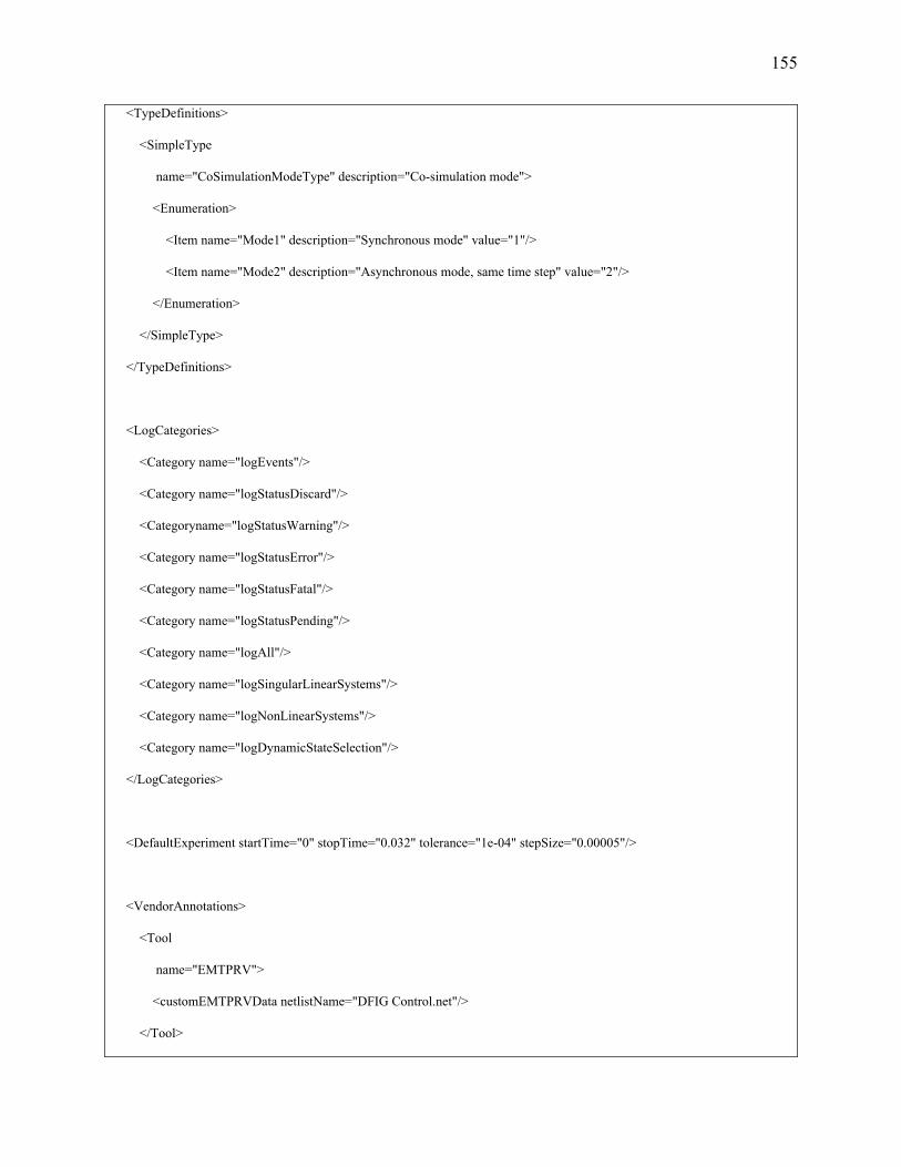
155

<TypeDefinitions>

<SimpleType

name="CoSimulationModeType" description="Co-simulation mode">

<Enumeration>

<Item name="Mode1" description="Synchronous mode" value="1"/>

<Item name="Mode2" description="Asynchronous mode, same time step" value="2"/>

</Enumeration>

</SimpleType>

</TypeDefinitions>

<LogCategories>

<Category name="logEvents"/>

<Category name="logStatusDiscard"/>

<Categoryname="logStatusWarning"/>

<Category name="logStatusError"/>

<Category name="logStatusFatal"/>

<Category name="logStatusPending"/>

<Category name="logAll"/>

<Category name="logSingularLinearSystems"/>

<Category name="logNonLinearSystems"/>

<Category name="logDynamicStateSelection"/>

</LogCategories>

<DefaultExperiment startTime="0" stopTime="0.032" tolerance="1e-04" stepSize="0.00005"/>

<VendorAnnotations>

<Tool

name="EMTPRV">

<customEMTPRVData netlistName="DFIG Control.net"/>

</Tool>

156

</VendorAnnotations>

<ModelVariables>

<ScalarVariable name="w_rotor_rads" valueReference="0" description="Description..." initial="approx"

variability="continuous" causality="input"><Real start="0.0"/></ScalarVariable>

<ScalarVariable name="Vdc_V" valueReference="1" description="Description..." initial="approx"


<ScalarVariable name="Iabc_converter_A_Ia" valueReference="2" description="Description..." initial="approx"


<ScalarVariable name="Iabc_converter_A_Ib" valueReference="3" description="Description..." initial="approx"


<ScalarVariable name="Iabc_converter_A_Ic" valueReference="4" description="Description..." initial="approx"


<ScalarVariable name="Iabc_Stator_A_Ia" valueReference="5" description="Description..." initial="approx"


<ScalarVariable name="Iabc_Stator_A_Ib" valueReference="6" description="Description..." initial="approx"


<ScalarVariable name="Iabc_Stator_A_Ic" valueReference="7" description="Description..." initial="approx"


<ScalarVariable name="Iabc_Rotor_A_Ia" valueReference="8" description="Description..." initial="approx"


<ScalarVariable name="Iabc_Rotor_A_Ib" valueReference="9" description="Description..." initial="approx"


<ScalarVariable name="Iabc_Rotor_A_Ic" valueReference="10" description="Description..." initial="approx"


<ScalarVariable name="Iabc_Grid_A_Ia" valueReference="11" description="Description..." initial="approx"


<ScalarVariable name="Iabc_Grid_A_Ib" valueReference="12" description="Description..." initial="approx"


<ScalarVariable name="Iabc_Grid_A_Ic" valueReference="13" description="Description..." initial="approx"


<ScalarVariable name="Vabc_Grid_A_Va" valueReference="14" description="Description..." initial="approx"


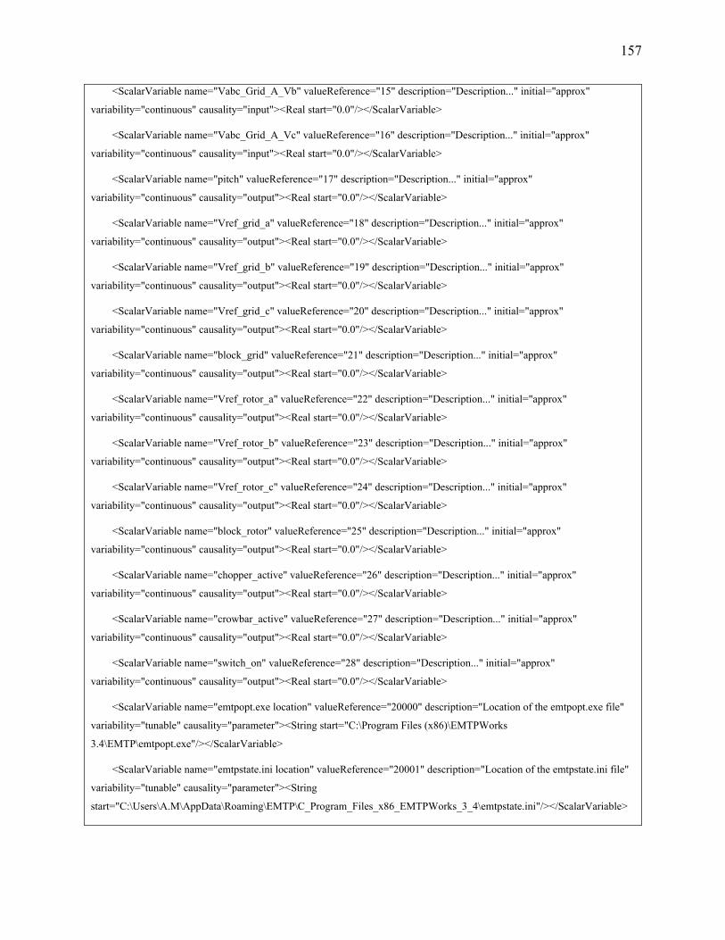
157

<ScalarVariable name="Vabc_Grid_A_Vb" valueReference="15" description="Description..." initial="approx"


<ScalarVariable name="Vabc_Grid_A_Vc" valueReference="16" description="Description..." initial="approx"


<ScalarVariable name="pitch" valueReference="17" description="Description..." initial="approx"

variability="continuous" causality="output"><Real start="0.0"/></ScalarVariable>

<ScalarVariable name="Vref_grid_a" valueReference="18" description="Description..." initial="approx"


<ScalarVariable name="Vref_grid_b" valueReference="19" description="Description..." initial="approx"


<ScalarVariable name="Vref_grid_c" valueReference="20" description="Description..." initial="approx"


<ScalarVariable name="block_grid" valueReference="21" description="Description..." initial="approx"


<ScalarVariable name="Vref_rotor_a" valueReference="22" description="Description..." initial="approx"


<ScalarVariable name="Vref_rotor_b" valueReference="23" description="Description..." initial="approx"


<ScalarVariable name="Vref_rotor_c" valueReference="24" description="Description..." initial="approx"


<ScalarVariable name="block_rotor" valueReference="25" description="Description..." initial="approx"


<ScalarVariable name="chopper_active" valueReference="26" description="Description..." initial="approx"


<ScalarVariable name="crowbar_active" valueReference="27" description="Description..." initial="approx"


<ScalarVariable name="switch_on" valueReference="28" description="Description..." initial="approx"


<ScalarVariable name="emtpopt.exe location" valueReference="20000" description="Location of the emtpopt.exe file"

variability="tunable" causality="parameter"><String start="C:\Program Files (x86)\EMTPWorks

3.4\EMTP\emtpopt.exe"/></ScalarVariable>

<ScalarVariable name="emtpstate.ini location" valueReference="20001" description="Location of the emtpstate.ini file"

variability="tunable" causality="parameter"><String

start="C:\Users\A.M\AppData\Roaming\EMTP\C_Program_Files_x86_EMTPWorks_3_4\emtpstate.ini"/></ScalarVariable>

158

<ScalarVariable name="Co-simulation mode" valueReference="20002" description="List of available Co-simulation

modes" variability="tunable" causality="parameter"><Enumeration

start="1"declaredType="CoSimulationModeType"/></ScalarVariable>

<ScalarVariable name="Time Out (ms)" valueReference="20003" description="Maximal time for synchronisation of the

co-simulation" variability="tunable" causality="parameter"><Integer start="5000" min="2000"/></ScalarVariable>

</ModelVariables>

<ModelStructure>

</ModelStructure>

</fmiModelDescription>

159

APPENDIX B – DETAILED IMPLEMENTATION OF FUNCITONS

COORDINATING MASTER-SLAVE CO-SIMULATION

The detailed implementation of functions fmi2DoStep (in file FMI2_Link_Master) and stepFunc

(in file FMI2_Device_Master) is presented in this appendix. It is noted that these two functions are

directly involved in coordinating the co-simulation between master and slaves.

• fmi2DoStep

fmi2Status fmi2DoStep(fmi2Component c, fmi2Real currentCommunicationPoint, fmi2Real communicationStepSize, fmi2Boolean noSetFMUStatePriorToCurrentPoint) { ModelInstance *comp = (ModelInstance *)c; if (invalidState(comp, "fmi2DoStep", modelInitialized | modelStepping)) return fmi2Error; comp->state = modelStepping; int nbIter = 0; double time_slave; double step_slave; FILTERED_LOG(comp, fmi2OK, logAll, "fmi2DoStep: " "time out = %i," "mode slave = %i," "currentCommunicationPoint = %g, " "communicationStepSize = %g, " "noSetFMUStatePriorToCurrentPoint = fmi%s", comp->timeOut,comp->SlaveMode,currentCommunicationPoint, communicationStepSize, noSetFMUStatePriorToCurrentPoint ? "True" : "False") if (communicationStepSize <= 0) { FILTERED_LOG(comp, fmi2Error, logStatusError, "fmi2DoStep: communication step size must be > 0. Found %g.", communicationStepSize) return fmi2Error; } setValueInInOutVector(tab_index_MasterTime,currentCommunicationPoint,comp); setValueInInOutVector(tab_index_MasterStep,communicationStepSize,comp); time_slave = getValueFromInOutVector(tab_index_SlaveTime,comp); step_slave = getValueFromInOutVector(tab_index_SlaveStep,comp); FILTERED_LOG(comp, fmi2OK, logAll, "fmi2DoStep: " "time slave = %g," "time master = %g,", getValueFromInOutVector(tab_index_SlaveTime,comp), getValueFromInOutVector(tab_index_MasterTime,comp)); if ((comp->SlaveMode == SlaveSynchrone)) { while(time_slave<currentCommunicationPoint+0.95*communicationStepSize) {

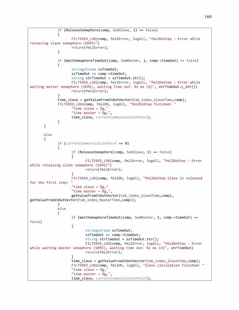
160

if (ReleaseSemaphore(comp, SemSlave, 1) == false) { FILTERED_LOG(comp, fmi2Error, logAll, "fmi2DoStep : Error while releasing slave semaphore (SEM3)") return(fmi2Error); } if (WaitSemaphoreTimeOut(comp, SemMaster, 1, comp->timeOut) == false) { stringstream ssTimeOut; ssTimeOut << comp->timeOut; string strTimeOut = ssTimeOut.str(); FILTERED_LOG(comp, fmi2Error, logAll, "fmi2DoStep : Error while waiting master semaphore (SEM2), waiting time out: %s ms (b)", strTimeOut.c_str()) return(fmi2Error); } time_slave = getValueFromInOutVector(tab_index_SlaveTime,comp); FILTERED_LOG(comp, fmi2OK, logAll, "fmi2DoStep finished: " "time slave = %g," "time master = %g,", time_slave, currentCommunicationPoint); } } else { if (currentCommunicationPoint == 0) { if (ReleaseSemaphore(comp, SemSlave, 1) == false) { FILTERED_LOG(comp, fmi2Error, logAll, "fmi2DoStep : Error while releasing slave semaphore (SEM3)") return(fmi2Error); } FILTERED_LOG(comp, fmi2OK, logAll, "fmi2DoStep Slave is released for the first step: " "time slave = %g," "time master = %g,", getValueFromInOutVector(tab_index_SlaveTime,comp), getValueFromInOutVector(tab_index_MasterTime,comp)); } else { if (WaitSemaphoreTimeOut(comp, SemMaster, 1, comp->timeOut) == false) { stringstream ssTimeOut; ssTimeOut << comp->timeOut; string strTimeOut = ssTimeOut.str(); FILTERED_LOG(comp, fmi2Error, logAll, "fmi2DoStep : Error while waiting master semaphore (SEM2), waiting time out: %s ms (d)", strTimeOut) return(fmi2Error); } time_slave = getValueFromInOutVector(tab_index_SlaveTime,comp); FILTERED_LOG(comp, fmi2OK, logAll, "Slave calculation finished: " "time slave = %g," "time master = %g,", time_slave, currentCommunicationPoint);

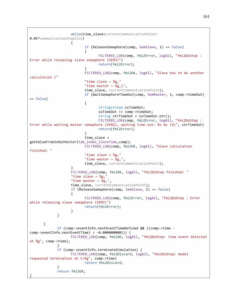
161

while(time_slave<currentCommunicationPoint-0.05*communicationStepSize) { if (ReleaseSemaphore(comp, SemSlave, 1) == false) { FILTERED_LOG(comp, fmi2Error, logAll, "fmi2DoStep : Error while releasing slave semaphore (SEM3)") return(fmi2Error); } FILTERED_LOG(comp, fmi2OK, logAll, "Slave has to do another calculation (" "time slave = %g," "time master = %g,)", time_slave, currentCommunicationPoint); if (WaitSemaphoreTimeOut(comp, SemMaster, 1, comp->timeOut) == false) { stringstream ssTimeOut; ssTimeOut << comp->timeOut; string strTimeOut = ssTimeOut.str(); FILTERED_LOG(comp, fmi2Error, logAll, "fmi2DoStep : Error while waiting master semaphore (SEM2), waiting time out: %s ms (d)", strTimeOut) return(fmi2Error); } time_slave = getValueFromInOutVector(tab_index_SlaveTime,comp); FILTERED_LOG(comp, fmi2OK, logAll, "Slave calculation finished: " "time slave = %g," "time master = %g,", time_slave, currentCommunicationPoint); } FILTERED_LOG(comp, fmi2OK, logAll, "fmi2DoStep finished: " "time slave = %g," "time master = %g,", time_slave, currentCommunicationPoint); if (ReleaseSemaphore(comp, SemSlave, 1) == false) { FILTERED_LOG(comp, fmi2Error, logAll, "fmi2DoStep : Error while releasing slave semaphore (SEM3)") return(fmi2Error); } } } if (comp->eventInfo.nextEventTimeDefined && ((comp->time - comp->eventInfo.nextEventTime) > -0.0000000001)) { FILTERED_LOG(comp, fmi2OK, logAll, "fmi2DoStep: time event detected at %g", comp->time); } if (comp->eventInfo.terminateSimulation) { FILTERED_LOG(comp, fmi2Discard, logAll, "fmi2DoStep: model requested termination at t=%g", comp->time) return fmi2Discard; } return fmi2OK; }

162

• stepFunc

void EMTPDevice::stepFunc(double *simulation_Time_Point,int *procedure_type, double *inputs_u, double *outputs_y) { double timeNow = this->EMTPData.simTime->t; int mainCtr, realCtr, intCtr, stringCtr, boolCtr; mainCtr = realCtr = intCtr = stringCtr = boolCtr = 0; this->isNewTime = (this->oldTime < timeNow); fmi2Status status; string errorMsg; if (timeNow == 0) { if (this->isNewTime) { status = this->fmi2EnterInitializationMode(this->s1); if (status == fmi2Error){ errorMsg = Def_Error_Msg15b; this->sendError(errorMsg, true); return; } this->flagInit = true; status = this->setIN(); if (status == fmi2Error) return; status = this->setINIE(); if (status == fmi2Error) return; if (!(this->noInitializationOfInputOutput)) { status = this->setFMUInput(inputs_u); if (status == fmi2Error) { return; } } for(int i = 0 ; i< this->nInputs; i++) this->prev_inputs[i] = inputs_u[i]; if (!(this->noInitializationOfInputOutput)) { status = this->getFMUOutputs(); if (status == fmi2Error) { return; } } } else { if (!(this->noInitializationOfInputOutput)) { status = this->setFMUInput(inputs_u); if (status == fmi2Error) { return;

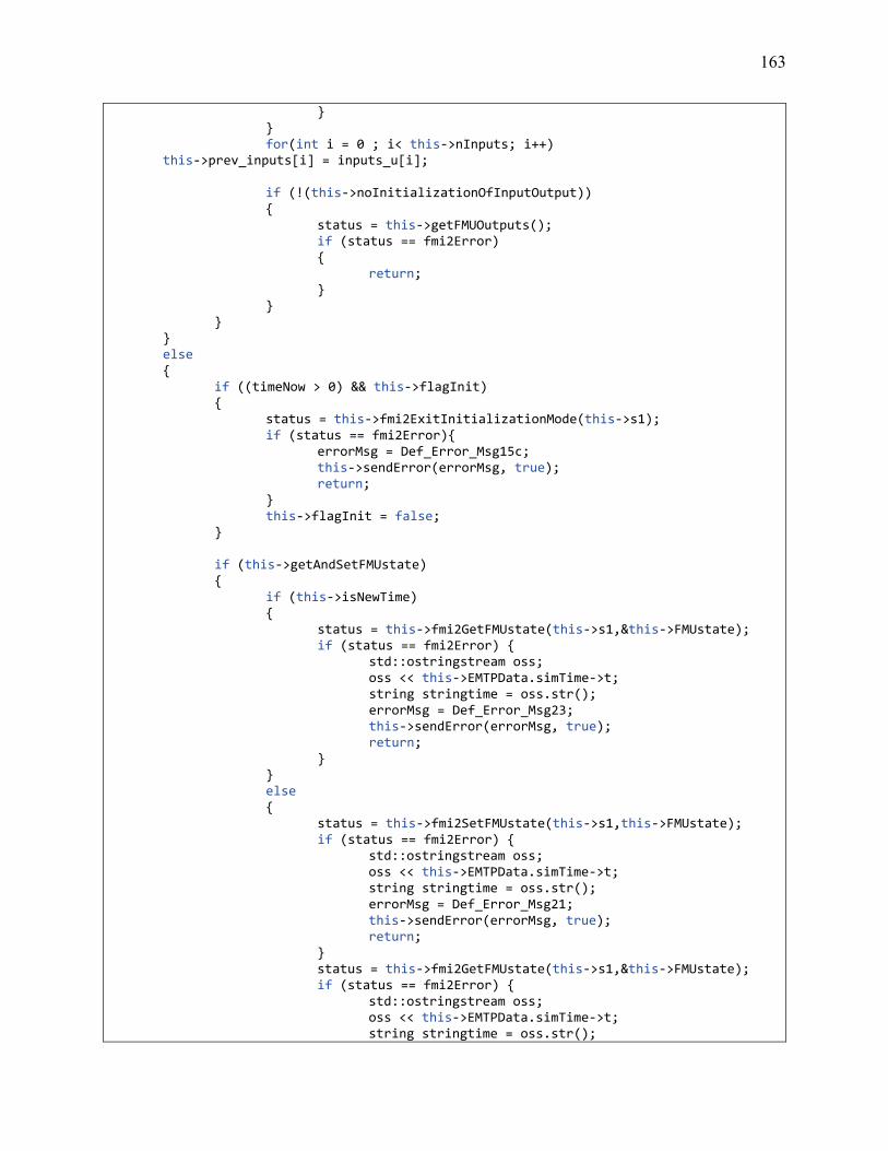
163

} } for(int i = 0 ; i< this->nInputs; i++) this->prev_inputs[i] = inputs_u[i]; if (!(this->noInitializationOfInputOutput)) { status = this->getFMUOutputs(); if (status == fmi2Error) { return; } } } } else { if ((timeNow > 0) && this->flagInit) { status = this->fmi2ExitInitializationMode(this->s1); if (status == fmi2Error){ errorMsg = Def_Error_Msg15c; this->sendError(errorMsg, true); return; } this->flagInit = false; } if (this->getAndSetFMUstate) { if (this->isNewTime) { status = this->fmi2GetFMUstate(this->s1,&this->FMUstate); if (status == fmi2Error) { std::ostringstream oss; oss << this->EMTPData.simTime->t; string stringtime = oss.str(); errorMsg = Def_Error_Msg23; this->sendError(errorMsg, true); return; } } else { status = this->fmi2SetFMUstate(this->s1,this->FMUstate); if (status == fmi2Error) { std::ostringstream oss; oss << this->EMTPData.simTime->t; string stringtime = oss.str(); errorMsg = Def_Error_Msg21; this->sendError(errorMsg, true); return; } status = this->fmi2GetFMUstate(this->s1,&this->FMUstate); if (status == fmi2Error) { std::ostringstream oss; oss << this->EMTPData.simTime->t; string stringtime = oss.str();

164

errorMsg = Def_Error_Msg23; this->sendError(errorMsg, true); return; } } fmi2Real currentCommunicationPoint = this->EMTPData.simTime->prev_t; fmi2Real communicationStepSize = this->EMTPData.simTime->t - this->EMTPData.simTime->prev_t; if (this->canHandleVariableCommunicationStepSize) { status = this->doStep(currentCommunicationPoint,communicationStepSize,inputs_u); if (status == fmi2Error) { return; } } else if (fabs((this->EMTPData.simTime->t - this->slaveTime - this->EMTPData.simTime->dt)/this->EMTPData.simTime->dt) < 0.00001) { status = this->doStep(this->slaveTime,communicationStepSize,inputs_u); if (status == fmi2Error) { return; } this->slaveTime = this->slaveTime+communicationStepSize; } } else if (handleVariableCommunicationStepSize) { fmi2Real currentCommunicationPoint = this->oldTime; fmi2Real communicationStepSize = timeNow - this->oldTime; status = this->doStep(currentCommunicationPoint,communicationStepSize,inputs_u); if (status == fmi2Error) { return; } } else { if (isNewTime){ if (this->canHandleVariableCommunicationStepSize) { if(this->oldTime > 0) { fmi2Real currentCommunicationPoint = this->previousCommunicationPoint; fmi2Real communicationStepSize = this->previousStepSize; status = this->doStep(currentCommunicationPoint,communicationStepSize,prev_inputs); if (status == fmi2Error) {

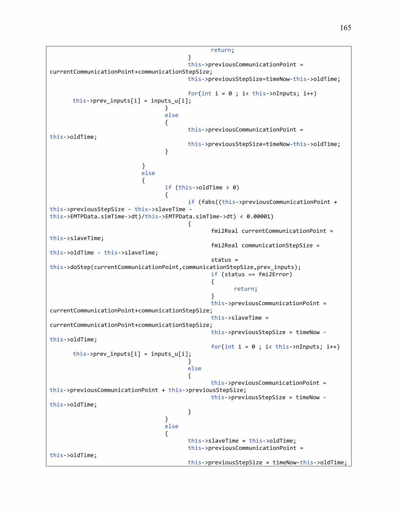
165

return; } this->previousCommunicationPoint = currentCommunicationPoint+communicationStepSize; this->previousStepSize=timeNow-this->oldTime; for(int i = 0 ; i< this->nInputs; i++) this->prev_inputs[i] = inputs_u[i]; } else { this->previousCommunicationPoint = this->oldTime; this->previousStepSize=timeNow-this->oldTime; } } else { if (this->oldTime > 0) { if (fabs((this->previousCommunicationPoint + this->previousStepSize - this->slaveTime - this->EMTPData.simTime->dt)/this->EMTPData.simTime->dt) < 0.00001) { fmi2Real currentCommunicationPoint = this->slaveTime; fmi2Real communicationStepSize = this->oldTime - this->slaveTime; status = this->doStep(currentCommunicationPoint,communicationStepSize,prev_inputs); if (status == fmi2Error) { return; } this->previousCommunicationPoint = currentCommunicationPoint+communicationStepSize; this->slaveTime = currentCommunicationPoint+communicationStepSize; this->previousStepSize = timeNow - this->oldTime; for(int i = 0 ; i< this->nInputs; i++) this->prev_inputs[i] = inputs_u[i]; } else { this->previousCommunicationPoint = this->previousCommunicationPoint + this->previousStepSize; this->previousStepSize = timeNow - this->oldTime; } } else { this->slaveTime = this->oldTime; this->previousCommunicationPoint = this->oldTime; this->previousStepSize = timeNow-this->oldTime;

166

} } } } } this->oldTime = timeNow; for(int i=0;i<nOutputs;i++) outputs_y[i] = this->outputs[i]; }

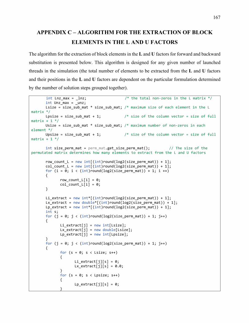
167

APPENDIX C – ALGORITHM FOR THE EXTRACTION OF BLOCK

ELEMENTS IN THE L AND U FACTORS

The algorithm for the extraction of block elements in the L and U factors for forward and backward

substitution is presented below. This algorithm is designed for any given number of launched

threads in the simulation (the total number of elements to be extracted from the L and U factors

and their positions in the L and U factors are dependent on the particular formulation determined

by the number of solution steps grouped together).

int Lnz_max = _lnz; /* the total non-zeros in the L matrix */ int Unz_max = _unz; Lsize = size_sub_mat * size_sub_mat; /* maximum size of each element in the L matrix */ Lpsize = size_sub_mat + 1; /* size of the column vector = size of full matrix + 1 */ Usize = size_sub_mat * size_sub_mat; /* maximum number of non-zeros in each element */ Upsize = size_sub_mat + 1; /* size of the column vector = size of full matrix + 1 */ int size_perm_mat = perm_mat.get_size_perm_mat(); // The size of the permutated matrix determines how many elements to extract from the L and U factors row_count_L = new int[(int)round(log2(size_perm_mat)) + 1]; col_count_L = new int[(int)round(log2(size_perm_mat)) + 1]; for (i = 0; i < (int)round(log2(size_perm_mat)) + 1; i ++) { row_count_L[i] = 0; col_count_L[i] = 0; } Li_extract = new int*[(int)round(log2(size_perm_mat)) + 1]; Lx_extract = new double*[(int)round(log2(size_perm_mat)) + 1]; Lp_extract = new int*[(int)round(log2(size_perm_mat)) + 1]; int s; for (j = 0; j < (int)round(log2(size_perm_mat)) + 1; j++) { Li_extract[j] = new int[Lsize]; Lx_extract[j] = new double[Lsize]; Lp_extract[j] = new int[Lpsize]; } for (j = 0; j < (int)round(log2(size_perm_mat)) + 1; j++) { for (s = 0; s < Lsize; s++) { Li_extract[j][s] = 0; Lx_extract[j][s] = 0.0; } for (s = 0; s < Lpsize; s++) { Lp_extract[j][s] = 0; }

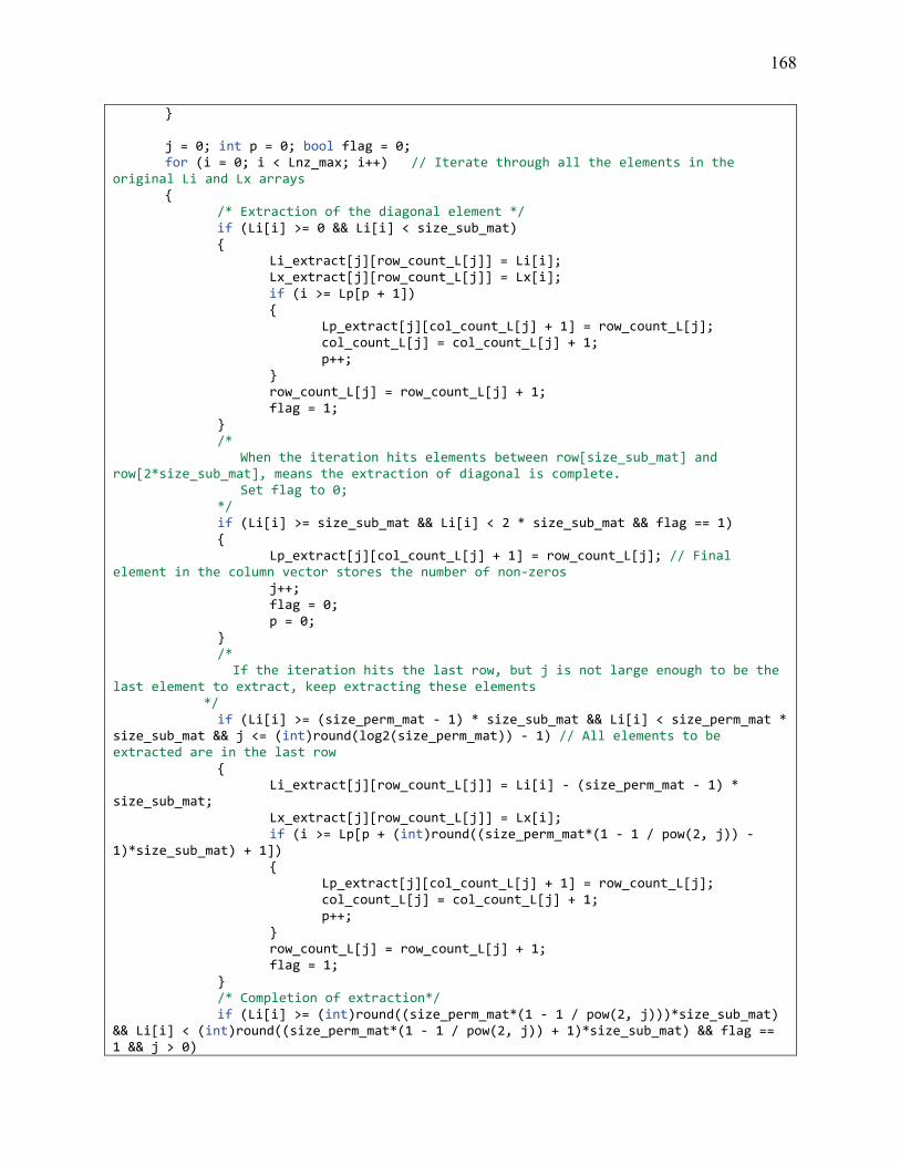
168

} j = 0; int p = 0; bool flag = 0; for (i = 0; i < Lnz_max; i++) // Iterate through all the elements in the original Li and Lx arrays { /* Extraction of the diagonal element */ if (Li[i] >= 0 && Li[i] < size_sub_mat) { Li_extract[j][row_count_L[j]] = Li[i]; Lx_extract[j][row_count_L[j]] = Lx[i]; if (i >= Lp[p + 1]) { Lp_extract[j][col_count_L[j] + 1] = row_count_L[j]; col_count_L[j] = col_count_L[j] + 1; p++; } row_count_L[j] = row_count_L[j] + 1; flag = 1; } /* When the iteration hits elements between row[size_sub_mat] and row[2*size_sub_mat], means the extraction of diagonal is complete. Set flag to 0; */ if (Li[i] >= size_sub_mat && Li[i] < 2 * size_sub_mat && flag == 1) { Lp_extract[j][col_count_L[j] + 1] = row_count_L[j]; // Final element in the column vector stores the number of non-zeros j++; flag = 0; p = 0; } /* If the iteration hits the last row, but j is not large enough to be the last element to extract, keep extracting these elements */ if (Li[i] >= (size_perm_mat - 1) * size_sub_mat && Li[i] < size_perm_mat * size_sub_mat && j <= (int)round(log2(size_perm_mat)) - 1) // All elements to be extracted are in the last row { Li_extract[j][row_count_L[j]] = Li[i] - (size_perm_mat - 1) * size_sub_mat; Lx_extract[j][row_count_L[j]] = Lx[i]; if (i >= Lp[p + (int)round((size_perm_mat*(1 - 1 / pow(2, j)) - 1)*size_sub_mat) + 1]) { Lp_extract[j][col_count_L[j] + 1] = row_count_L[j]; col_count_L[j] = col_count_L[j] + 1; p++; } row_count_L[j] = row_count_L[j] + 1; flag = 1; } /* Completion of extraction*/ if (Li[i] >= (int)round((size_perm_mat*(1 - 1 / pow(2, j)))*size_sub_mat) && Li[i] < (int)round((size_perm_mat*(1 - 1 / pow(2, j)) + 1)*size_sub_mat) && flag == 1 && j > 0)

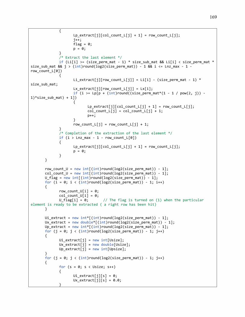
169

{ Lp_extract[j][col_count_L[j] + 1] = row_count_L[j]; j++; flag = 0; p = 0; } /* Extract the last element */ if (Li[i] >= (size_perm_mat - 1) * size_sub_mat && Li[i] < size_perm_mat * size_sub_mat && j > (int)round(log2(size_perm_mat)) - 1 && i <= Lnz_max - 1 - row_count_L[0]) { Li_extract[j][row_count_L[j]] = Li[i] - (size_perm_mat - 1) * size_sub_mat; Lx_extract[j][row_count_L[j]] = Lx[i]; if (i >= Lp[p + (int)round((size_perm_mat*(1 - 1 / pow(2, j)) - 1)*size_sub_mat) + 1]) { Lp_extract[j][col_count_L[j] + 1] = row_count_L[j]; col_count_L[j] = col_count_L[j] + 1; p++; } row_count_L[j] = row_count_L[j] + 1; } /* Completion of the extraction of the last element */ if (i > Lnz_max - 1 - row_count_L[0]) { Lp_extract[j][col_count_L[j] + 1] = row_count_L[j]; p = 0; } } row_count_U = new int[(int)round(log2(size_perm_mat)) - 1]; col_count_U = new int[(int)round(log2(size_perm_mat)) - 1]; U_flag = new int[(int)round(log2(size_perm_mat)) - 1]; for (i = 0; i < (int)round(log2(size_perm_mat)) - 1; i++) { row_count_U[i] = 0; col_count_U[i] = 0; U_flag[i] = 0; // The flag is turned on (1) when the particular element is ready to be extracted ( a right row has been hit) } Ui_extract = new int*[(int)round(log2(size_perm_mat)) - 1]; Ux_extract = new double*[(int)round(log2(size_perm_mat)) - 1]; Up_extract = new int*[(int)round(log2(size_perm_mat)) - 1]; for (j = 0; j < (int)round(log2(size_perm_mat)) - 1; j++) { Ui_extract[j] = new int[Usize]; Ux_extract[j] = new double[Usize]; Up_extract[j] = new int[Upsize]; } for (j = 0; j < (int)round(log2(size_perm_mat)) - 1; j++) { for (s = 0; s < Usize; s++) { Ui_extract[j][s] = 0; Ux_extract[j][s] = 0.0; }

170

for (s = 0; s < Upsize; s++) { Up_extract[j][s] = 0; } } j = 0; int m = 3; p = 0; for (i = 0; i < Unz_max; i++) { if (Ui[i] >= (int)round((size_perm_mat*(1 - 1 / pow(2, j + 1)) - 1))*size_sub_mat && Ui[i] < (int)round((size_perm_mat*(1 - 1 / pow(2, j + 1))))*size_sub_mat && j < (int)round(log2(size_perm_mat)) -2) { U_flag[j] = 1; } /* Extract the first element*/ if (j == 0 && Ui[i] >= size_sub_mat && Ui[i] < 2 * size_sub_mat && U_flag[j] == 1) { Ui_extract[j][row_count_U[j]] = Ui[i] - size_sub_mat; Ux_extract[j][row_count_U[j]] = Ux[i]; if (i >= Up[p + (int)round((size_perm_mat*(1 - 1 / pow(2, j + 1))))*size_sub_mat + 1]) { Up_extract[j][col_count_U[j] + 1] = row_count_U[j]; col_count_U[j] = col_count_U[j] + 1; p++; } row_count_U[j] = row_count_U[j] + 1; } /* Extract U2, U3, etc */ if (Ui[i] >= (2 + (int)round(size_perm_mat*(1 - 1 / pow(2, j))) - 1)*size_sub_mat && Ui[i] < (2 + (int)round(size_perm_mat*(1 - 1 / pow(2, j))))*size_sub_mat && j > 0 && j < (int)round(log2(size_perm_mat)) - 2 && U_flag[j] == 1) { Ui_extract[j][row_count_U[j]] = Ui[i] - (2 + (int)round(size_perm_mat*(1 - 1 / pow(2, j))) - 1)*size_sub_mat; Ux_extract[j][row_count_U[j]] = Ux[i]; if (i >= Up[p + (int)round((size_perm_mat*(1 - 1 / pow(2, j + 1))))*size_sub_mat + 1]) { Up_extract[j][col_count_U[j] + 1] = row_count_U[j]; col_count_U[j] = col_count_U[j] + 1; p++; } row_count_U[j] = row_count_U[j] + 1; } /* Mark the completion of an extraction */ if (U_flag[j] == 1 && Ui[i] >= m * size_sub_mat && Ui[i] < (m + 1) * size_sub_mat) { Up_extract[j][col_count_U[j] + 1] = row_count_U[j]; j++; m = 2 * m; p = 0; } /* Mark the extraction of the last element is ready */

171

if (j == (int)round(log2(size_perm_mat)) - 2 && Ui[i] >= ((int)size_perm_mat / 4 + 1 - 1) * size_sub_mat && Ui[i] < ((int)size_perm_mat / 4 + 1) * size_sub_mat) { U_flag[j] = 1; } /* Extraction the last element */ if (j == (int)round(log2(size_perm_mat)) - 2 && U_flag[j] == 1 && Ui[i] >= (size_perm_mat - 2 - 1) * size_sub_mat && Ui[i] < (size_perm_mat - 2) * size_sub_mat) { Ui_extract[j][row_count_U[j]] = Ui[i] - (size_perm_mat - 2 - 1) * size_sub_mat; Ux_extract[j][row_count_U[j]] = Ux[i]; if (i >= Up[p + (int)round((size_perm_mat*(1 - 1 / pow(2, j + 1))))*size_sub_mat + 1]) { Up_extract[j][col_count_U[j] + 1] = row_count_U[j]; col_count_U[j] = col_count_U[j] + 1; p++; } row_count_U[j] = row_count_U[j] + 1; } /* Mark the completion of the extraction of the last element */ if (j == (int)round(log2(size_perm_mat)) - 2 && Ui[i] >= (size_perm_mat - 1) * size_sub_mat && Ui[i] < size_perm_mat * size_sub_mat) { Up_extract[j][col_count_U[j] + 1] = row_count_U[j]; j++; } }

172

APPENDIX D – LIST OF PUBLICATIONS

The following is a list of journal and conference papers that are derived from this Ph.D. project.

Journal publications

M. Cai, H. Gras, J. Mahseredjian, E. Rutovic, A. El-Akoum, “Functional Mock-up Interface-Based Approach for Parallel and Multistep Simulation of Electromagnetic Transients,” IEEE Trans. on Power Delivery, vol. 33, issue 6, pp. 2978-2988, Dec. 2018. M. Cai, J. Mahseredjian, U. Karaagac, A. El-Akoum, X. Fu, “Functional Mock-up Interface Based Parallel Multistep Approach with Signal Correction for Electromagnetic Transients Simulations, ” IEEE Trans. on Power Systems, vol. 34, issue 3, pp. 2482-2484, May 2019.

Conference publications

M. Cai, J. Mahseredjian, H. Gras, A. El-Akoum, X. Fu, “A Co-Simulation Based Parallel and

Multistep Approach for Accelerating EMT Simulations, ” International Conference on Power

Systems Transients (IPST), Perpignan, France, June 18-21, 2019.

M. Cai, J. Mahseredjian, A. Haddadi, X. Fu, “A Parallelization-in-time Approach for

Accelerating Power System EMT Simulations, ” Power Systems Computation Conference

(PSCC), Porto, Portugal, June 29-July 3, 2020, submitted.

A. Haddadi, M. Cai, U. Karaagac, J. Mahseredjian, “Power System Test Cases for EMT-type Simulation Studies,” International Conference on Power Systems Transients (IPST), Perpignan, France, June 18-21, 2019. X. Fu, S. M. Seye, J. Mahseredjian, M. Cai, C. Dufour, “A Comparison of Numerical Integration Methods and Discontinuity Treatment for EMT Simulations, ” Power System Computation Conference (PSCC), Dublin, Ireland, 2019. M. Cai, J. Mahseredjian, “A Parallel Numerical Method Based on the PIMIT for Fast Power System EMT Simulations, ” The 11th International Symposium on EMC and Transients in Infrastuctures, the 13th International Student Session (ISET/ISS), Kyoto, Japan, 2017.

parallel and multistep simulation of power system transients

Documents