Parallel Depth-First Search

for Directed Acyclic Graphs

Maxim Naumov1, Alysson Vrielink1,2, and Michael Garland1

1NVIDIA, 2701 San Tomas Expressway, Santa Clara, CA 950502Stanford University, 2575 Sand Hill Road, Menlo Park, CA, 94025

Abstract

Depth-First Search (DFS) is a pervasive algorithm, often used as a build-ing block for topological sort, connectivity and planarity testing, amongmany other applications. We propose a novel work-efficient parallel algo-rithm for the DFS traversal of directed acyclic graph (DAG). The algorithmtraverses the entire DAG in a BFS-like fashion no more than three times.As a result it finds the DFS pre-order (discovery) and post-order (finishtime) as well as the parent relationship associated with every node in aDAG. We analyse the runtime and work complexity of this novel parallelalgorithm. Also, we show that unlike many of its predecessors, our algo-rithm is easy to implement and optimize for performance. In particular, weshow that its CUDA implementation on the GPU outperforms sequentialDFS on the CPU by up to 6× in our experiments.

1 Introduction

Let a graph G = (V,E) be defined by its vertex V = {1, ..., n} and edge E ={(i1, j1), ..., (im, jm)} sets. Also, assume that it has n nodes and m edges.

The sequential depth-first search (DFS) algorithm was proposed in [25]. It isa pervasive algorithm, often used as a building block for topological sort [10, 18],connectivity and planarity testing [15, 28], among many other applications.

In the DFS traversal problem we are interested in finding parent, pre-orderand post-order for every node in a graph. For example, for the graph on Fig. 1

NVIDIA Technical Report NVR-2017-001, March 2017.c© 2017 NVIDIA Corporation. All rights reserved.

1

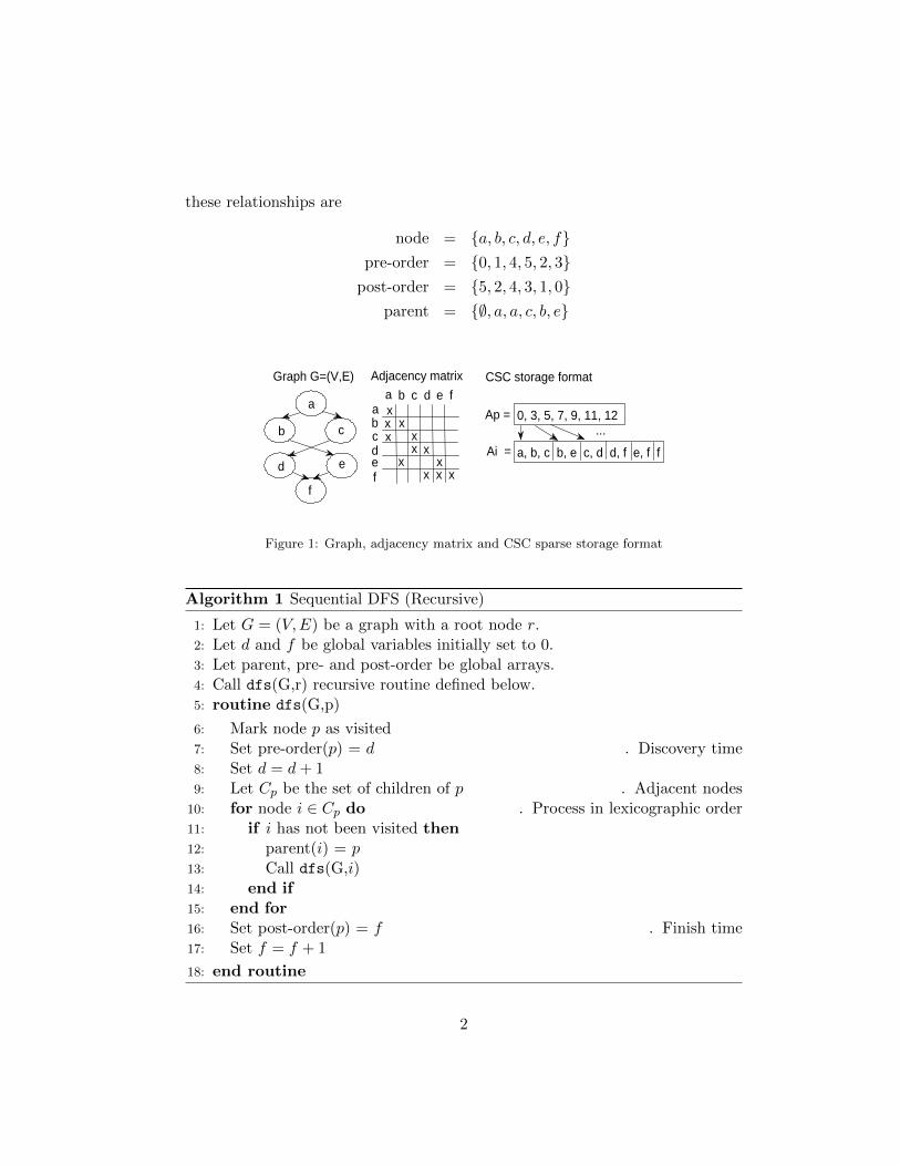
these relationships are

node = {a, b, c, d, e, f}pre-order = {0, 1, 4, 5, 2, 3}

post-order = {5, 2, 4, 3, 1, 0}parent = {∅, a, a, c, b, e}

xx

x

abcde

xx

xx

xf

a c d feb

xx

xx

Graph G=(V,E) CSC storage format

Ap = 0, 3, 5, 7, 9, 11, 12

Ai = a, b, c b, e c, d d, f e, f f

...

Adjacency matrix

c

d

b

f

e

a

Figure 1: Graph, adjacency matrix and CSC sparse storage format

Algorithm 1 Sequential DFS (Recursive)

1: Let G = (V,E) be a graph with a root node r.2: Let d and f be global variables initially set to 0.3: Let parent, pre- and post-order be global arrays.4: Call dfs(G,r) recursive routine defined below.5: routine dfs(G,p)

6: Mark node p as visited7: Set pre-order(p) = d . Discovery time8: Set d = d+ 19: Let Cp be the set of children of p . Adjacent nodes

10: for node i ∈ Cp do . Process in lexicographic order11: if i has not been visited then12: parent(i) = p13: Call dfs(G,i)14: end if15: end for16: Set post-order(p) = f . Finish time17: Set f = f + 1

18: end routine

2

The DFS traversal can be computed sequentially using many equivalent for-mulations of Alg. 1 [10]. Notice that unless stated otherwise, we assume that thechildren of a node are processed in some specified order, such as the lexicographicorder, as shown on line 10 in Alg. 1.

2 Related Work

There has been a significant effort to create a parallel variation of DFS algorithmin the past. The DFS on planar graphs has been considered in [14, 23, 24]. Inparticular, it has been shown in [23] that for such graphs it is possible to performa parallel DFS traversal in O(log2 n) time with n processors. On the other hand,the DFS on directed acyclic graphs (DAGs) has been considered in [13, 30], whereit has been shown that for such graphs it is possible to find the DFS traversalin O(log2 n) time with nω/ log n processors, where ω < 2.373 is the matrixmultiplication exponent. Also, the DFS on directed graphs with cycles has beenconsidered in [3, 4], where it has been shown that such traversal can be found inO(√n log11 n) time with n3 processors. Finally, a relaxation of the problem from

lexicographic to unordered DFS, where the children of a node are not requiredto be explored in lexicographic order, but the parent relationship should still besuch that it results in a DFS tree [17, 20, 22], has been explored for undirectedgraphs in [1, 2], where it has been shown that using randomized algorithms theunordered traversal can be obtained in O(log5 n) time with nω+1 processors.

Recall that a given problem is in class P if there is a constant α such thatthis problem can be solved in O(nα) time on a single processor. Also, a givenproblem is in class NC and RNC if there are constants α and β such that thisproblem can be solved in O(logα n) time on O(nβ) processors with deterministicand randomized algorithms, respectively [6]. It has been shown that the lexico-graphic DFS traversal problem for general graphs is P-complete, in other words,all problems in class P can be reduced to it [21]. Therefore, a parallel algorithmthat solves this problem in polylogarithmic time using polynomial number ofprocessors would imply that P = NC or RNC, which is unlikely. However,it is misleading to use this result to simply state that DFS is an inherentlysequential algorithm without specifying the taxonomy of the (lexicographic ver-sus unordered) type of the traversal and the (planar, directed or general) classof graphs we are working with. As shown by the scientific literature review, wemay conclude in particular that the lexicographic DFS traversal problem for pla-nar graphs and DAGs ∈ NC and unordered DFS traversal problem for generalgraphs ∈ RNC.

3

3 Contributions

Let us define a directed tree (DT) to be a DAG, where every node has a singleparent. We will show that in a DT finding pre-order (discovery) and post-order(finish time) of a node is equivalent to computing an offset based on the numberof nodes to the left and below yourself.

Also, we will propose two approaches for identifying the parent of a nodecorresponding to a lexicographic DFS of a DAG. The first will be based on thepath comparisons and second will rely on the solution of a single source shortestpath (SSSP) problem. We will use them to transform a DAG into a DT.

We will combine these results to develop a work-efficient parallel algorithmfor computing lexicographic DFS traversal of a DAG. The algorithm will traversethe entire DAG in parallel in a Breadth-First Search (BFS)-like fashion no morethan three times, with at least one traversal requiring that all edges to eachparent are visited prior to proceeding to its children. As a result it will obtainthe DFS parent, pre- and post-order relationship associated with every node.

We will show that for sparse graphs the parallel DFS can be performed inO(η log n) steps, where η is the length of the longest path between a root anda node. The length η depends on the connectivity structure of a graph. Itcan be short O(1), balanced O(log n) or long O(n) and we will propose severaloptimizations and a novel data structure that can effectively compress it.

Also, we will show that the work complexity of the proposed parallel DFSis O(m + n), matching that of the sequential algorithm. We point out that toachieve this work complexity bound the number of processors t ≤ m+n activelydoing work varies at each step of the algorithm.

Finally, we will show that unlike many of its predecessors, our algorithm iseasy to implement and optimize for performance. In particular, we will showthat its CUDA implementation on the GPU outperforms sequential DFS on theCPU by up to 6× in our experiments.

4 Algorithm

Let us assume that we are working with a DAG, in other words, a graph G =(V,E) that has directed edges and no cycles. The graph and its adjacency matrixcan be stored in arbitrary data structures. Suppose that we use the standardCSR/CSC format, which simply concatenates all non-zero entries of the matrixin row/column-major order and records the starting position for the entries ofeach row/column, see Fig. 1. Notice that this format allows us to easily traverseand access information associated with outgoing edges.

4

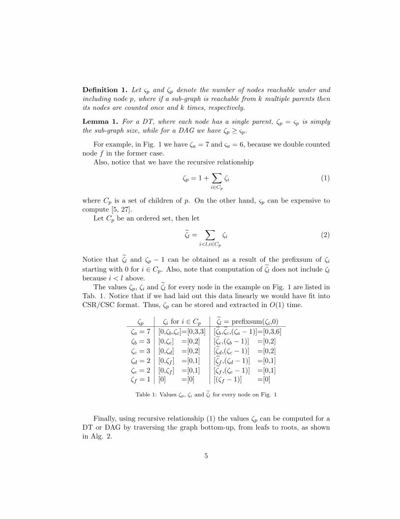
Definition 1. Let ςp and ζp denote the number of nodes reachable under andincluding node p, where if a sub-graph is reachable from k multiple parents thenits nodes are counted once and k times, respectively.

Lemma 1. For a DT, where each node has a single parent, ζp = ςp is simplythe sub-graph size, while for a DAG we have ζp ≥ ςp.

For example, in Fig. 1 we have ζa = 7 and ςa = 6, because we double countednode f in the former case.

Also, notice that we have the recursive relationship

ζp = 1 +∑i∈Cp

ζi (1)

where Cp is a set of children of p. On the other hand, ςp can be expensive tocompute [5, 27].

Let Cp be an ordered set, then let

ζ̃l =∑

i<l,i∈Cp

ζi (2)

Notice that ζ̃l and ζp − 1 can be obtained as a result of the prefixsum of ζistarting with 0 for i ∈ Cp. Also, note that computation of ζ̃l does not include ζlbecause i < l above.

The values ζp, ζi and ζ̃l for every node in the example on Fig. 1 are listed inTab. 1. Notice that if we had laid out this data linearly we would have fit intoCSR/CSC format. Thus, ζp can be stored and extracted in O(1) time.

ζp ζi for i ∈ Cp ζ̃l = prefixsum(ζi,0)

ζa = 7 [0,ζb,ζc]=[0,3,3] [ζ̃b,ζ̃c,(ζa − 1)]=[0,3,6]

ζb = 3 [0,ζe] =[0,2] [ζ̃e,(ζb − 1)] =[0,2]

ζc = 3 [0,ζd] =[0,2] [ζ̃d,(ζc − 1)] =[0,2]

ζd = 2 [0,ζf ] =[0,1] [ζ̃f ,(ζd − 1)] =[0,1]

ζe = 2 [0,ζf ] =[0,1] [ζ̃f ,(ζe − 1)] =[0,1]ζf = 1 [0] =[0] [(ζf − 1)] =[0]

Table 1: Values ζp, ζi and ζ̃l for every node on Fig. 1

Finally, using recursive relationship (1) the values ζp can be computed for aDT or DAG by traversing the graph bottom-up, from leafs to roots, as shownin Alg. 2.

5

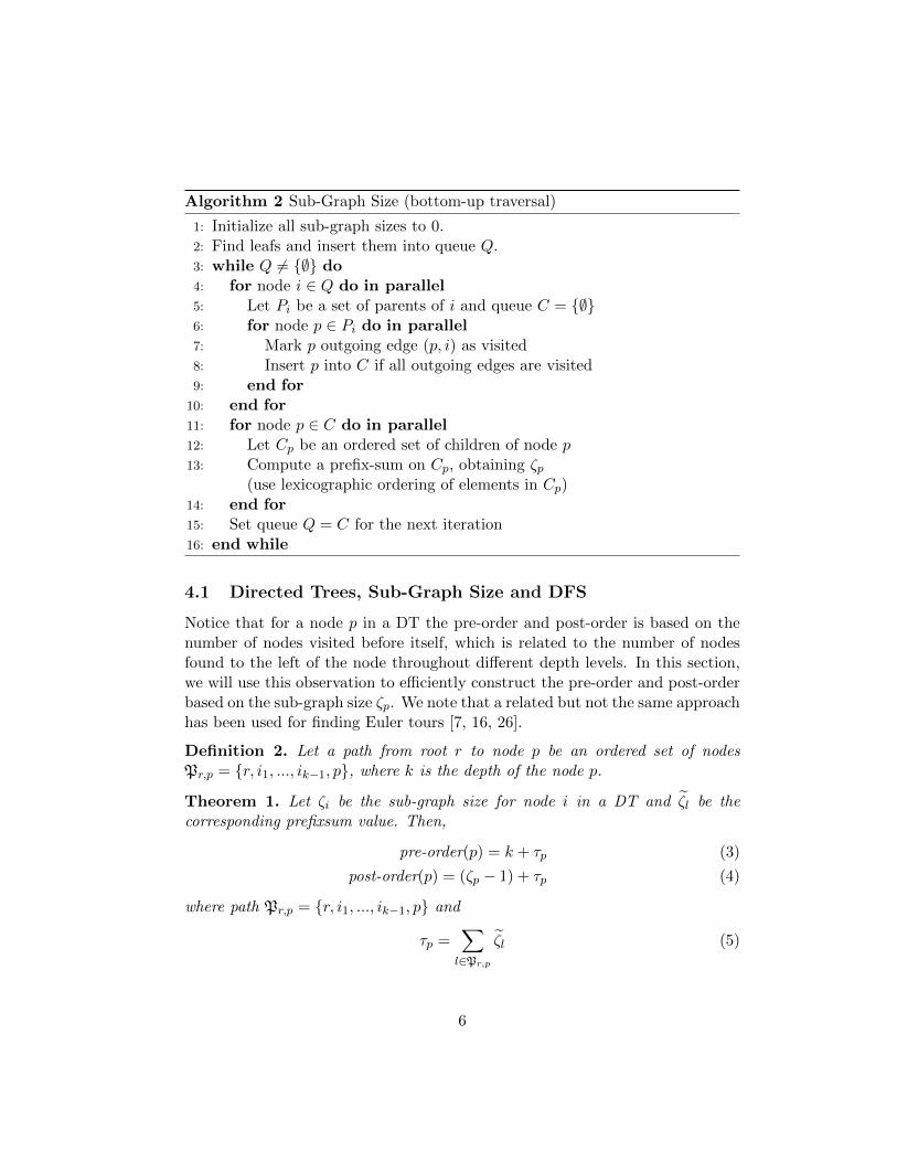
Algorithm 2 Sub-Graph Size (bottom-up traversal)

1: Initialize all sub-graph sizes to 0.2: Find leafs and insert them into queue Q.3: while Q 6= {∅} do4: for node i ∈ Q do in parallel5: Let Pi be a set of parents of i and queue C = {∅}6: for node p ∈ Pi do in parallel7: Mark p outgoing edge (p, i) as visited8: Insert p into C if all outgoing edges are visited9: end for

10: end for11: for node p ∈ C do in parallel12: Let Cp be an ordered set of children of node p13: Compute a prefix-sum on Cp, obtaining ζp

(use lexicographic ordering of elements in Cp)14: end for15: Set queue Q = C for the next iteration16: end while

4.1 Directed Trees, Sub-Graph Size and DFS

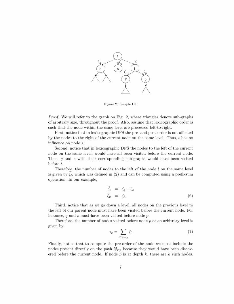
Notice that for a node p in a DT the pre-order and post-order is based on thenumber of nodes visited before itself, which is related to the number of nodesfound to the left of the node throughout different depth levels. In this section,we will use this observation to efficiently construct the pre-order and post-orderbased on the sub-graph size ζp. We note that a related but not the same approachhas been used for finding Euler tours [7, 16, 26].

Definition 2. Let a path from root r to node p be an ordered set of nodesPr,p = {r, i1, ..., ik−1, p}, where k is the depth of the node p.

Theorem 1. Let ζi be the sub-graph size for node i in a DT and ζ̃l be thecorresponding prefixsum value. Then,

pre-order(p) = k + τp (3)

post-order(p) = (ζp − 1) + τp (4)

where path Pr,p = {r, i1, ..., ik−1, p} and

τp =∑l∈Pr,p

ζ̃l (5)

6

r

q s t

h

ζq ζ

sζ

t

ζh

ζp

p

Figure 2: Sample DT

Proof. We will refer to the graph on Fig. 2, where triangles denote sub-graphsof arbitrary size, throughout the proof. Also, assume that lexicographic order issuch that the node within the same level are processed left-to-right.

First, notice that in lexicographic DFS the pre- and post-order is not affectedby the nodes to the right of the current node on the same level. Thus, t has noinfluence on node s.

Second, notice that in lexicographic DFS the nodes to the left of the currentnode on the same level, would have all been visited before the current node.Thus, q and s with their corresponding sub-graphs would have been visitedbefore t.

Therefore, the number of nodes to the left of the node l on the same levelis given by ζ̃l, which was defined in (2) and can be computed using a prefixsumoperation. In our example,

ζ̃t = ζq + ζs

ζ̃p = ζh (6)

Third, notice that as we go down a level, all nodes on the previous level tothe left of our parent node must have been visited before the current node. Forinstance, q and s must have been visited before node p.

Therefore, the number of nodes visited before node p at an arbitrary level isgiven by

τp =∑l∈Pr,p

ζ̃l (7)

Finally, notice that to compute the pre-order of the node we must include thenodes present directly on the path Pr,p because they would have been discov-ered before the current node. If node p is at depth k, there are k such nodes.

7

Therefore,pre-order(p) = k + τp (8)

On the other hand, to compute post-order of the node we must include thenodes under it because they would have been finished before the current node.Therefore,

post-order(p) = (ζp − 1) + τp (9)

Also, notice that τp can be computed recursively using the following result.

Corollary 1. Let a path from root r to node p be an ordered set of nodes Pr,ik ={r, i1, ..., ik−1, p}. Then,

τp = τik−1+ ζ̃p (10)

Therefore, using recursive relationship (10) the pre- and post-order can becomputed for a DT by traversing the graph top-down, from roots to leafs, andaccumulating the sub-graph size as shown in Alg. 3.

Algorithm 3 Pre- and Post-Order (top-down traversal)

1: Initialize pre and post-order of every node to 0.2: Find roots and insert them into queue Q.3: while Q 6= {∅} do4: for node p ∈ Q do in parallel5: Let pre = pre-order(p)6: Let post= post-order(p)7: Let Cp be a set of children of p and queue P = {∅}8: for node i ∈ Cp do in parallel

9: Set pre-order(i) = pre + ζ̃i10: Set post-order(i)= post+ ζ̃i11: Mark i incoming edge (p, i) as visited12: Insert i into P if all incoming edges are visited13: end for14: Set pre-order(p) = pre + depth(p)15: Set post-order(p)= post+ ζp16: end for17: Set queue Q = P for the next iteration18: end while

8

So far we have shown how to compute a DFS traversal of a DT using Alg.2 and 3. Next we will show how we can transform a DAG into a valid DTby selecting a single parent for every node, such that it corresponds to a DFStraversal. For this purpose we will develop Path- and SSSP-based complemen-tary variations of the algorithm.

4.2 Path-based DFS

In the Path-based DFS we obtain a DT from a DAG by keeping track of multiplepaths from root r to node p and selecting among them the DFS path accordingto the following rules.

Definition 3. Let Pr,p = {r, i1, i2, ..., ik−1, p} and Qr,p = {r, j1, j2, ..., jl−1, p} betwo paths of potentially different length to node p. We say that path Pr,p has thefirst lexicographically smallest node and denote it

Pr,p < Qr,p (11)

when during the pair-wise comparison of the elements in the two paths goingfrom left-to-right the path Pr,p has the lexicographically smallest element in thefirst mismatch.

For example, in Fig. 1 the two paths to node f are

Pa,f = [a, b, e, f ] (12)

Qa,f = [a, c, d, f ] (13)

When we compare these paths pairwise from left-to-right, we notice that thefirst mismatch between paths happens in the second pair [ bc ], where the lexico-graphically smallest digit b is contained in (12) and therefore we say that

Pa,f < Qa,f (14)

Notice that the next pairwise mismatch [ ed ], where the lexicographically smallestdigit d is contained in (13), does not affect this decision.

Theorem 2. Let Pr,p = [r, i1, i2, ..., ik−1, p] and Qr,p = [r, j1, j2, ..., jl−1, p] betwo paths to node p. If Pr,p < Qr,p then Pr,p is the path taken by DFS.

Proof. Let us prove the theorem by contradiction. Suppose Pr,p has the firstlexicographically smallest node left-to-right i at depth k, but path Qr,p is theone taken by DFS.

9

Notice that since i is the first lexicographically smallest node left-to-right,then all nodes preceding it in both paths must be the same. Also, notice that imust have been explored before the node at depth k in path Qr,p because it islexicographically smallest. Finally, notice that DFS always explores the entiresub-graph under a node before proceeding. Therefore, DFS would have visitedthe entire sub-graph under i, including node p, before it was visited from pathQr,p, which is a contradiction.

Corollary 2. Let S be the set of all paths from root r to node p. The DFStraversal takes

Pr,p = minQr,p∈S

Qr,p (15)

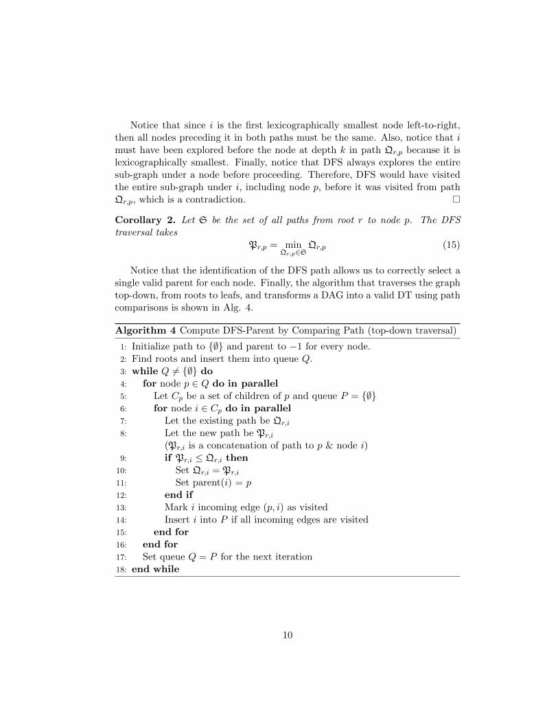
Notice that the identification of the DFS path allows us to correctly select asingle valid parent for each node. Finally, the algorithm that traverses the graphtop-down, from roots to leafs, and transforms a DAG into a valid DT using pathcomparisons is shown in Alg. 4.

Algorithm 4 Compute DFS-Parent by Comparing Path (top-down traversal)

1: Initialize path to {∅} and parent to −1 for every node.2: Find roots and insert them into queue Q.3: while Q 6= {∅} do4: for node p ∈ Q do in parallel5: Let Cp be a set of children of p and queue P = {∅}6: for node i ∈ Cp do in parallel7: Let the existing path be Qr,i

8: Let the new path be Pr,i

(Pr,i is a concatenation of path to p & node i)9: if Pr,i ≤ Qr,i then

10: Set Qr,i = Pr,i

11: Set parent(i) = p12: end if13: Mark i incoming edge (p, i) as visited14: Insert i into P if all incoming edges are visited15: end for16: end for17: Set queue Q = P for the next iteration18: end while

10

In a naive implementation, to perform the comparison on line 9 in Alg. 4, wecan store the path nodes in a linear array, align the arrays on the left and comparethe elements pairwise left-to-right until a mismatch is found between the twoarrays. In practice, the path length is between O(log n) and O(n) and therefore,in order to shorten it, we perform the following optimizations to minimize thestorage and comparison time requirements.

4.2.1 Path Static Pruning

Notice that when we look at two paths that reach the same node, there will bea parent p with outgoing edges (p, i) and (p, j) to nodes i and j, respectively,where one node will be preferred over the other due to its lexicographic ordering.It is the comparison of i and j stored in different paths in such a situation thatallows us to distinguish between them. On the other hand, parent nodes p witha single outgoing edge (p, i) will never be a decision point on which we preferone path over the other, because the path would have split before or after suchpoint, it simply can not split at it.

This reasoning allows us to conclude the following theorem, which impliesthat we do not need to store nodes in the path whose parents have single outgoingedge.

Theorem 3. If parent p has only a single outgoing edge (p, j) to node j then jdoes not need to be stored in the path, in other words, it will not affect the pathcomparison.

For example, using static pruning we may conclude that the two paths tonode f in Fig. 1 can be stored as

[a, b, f ] (16)

[a, c, f ] (17)

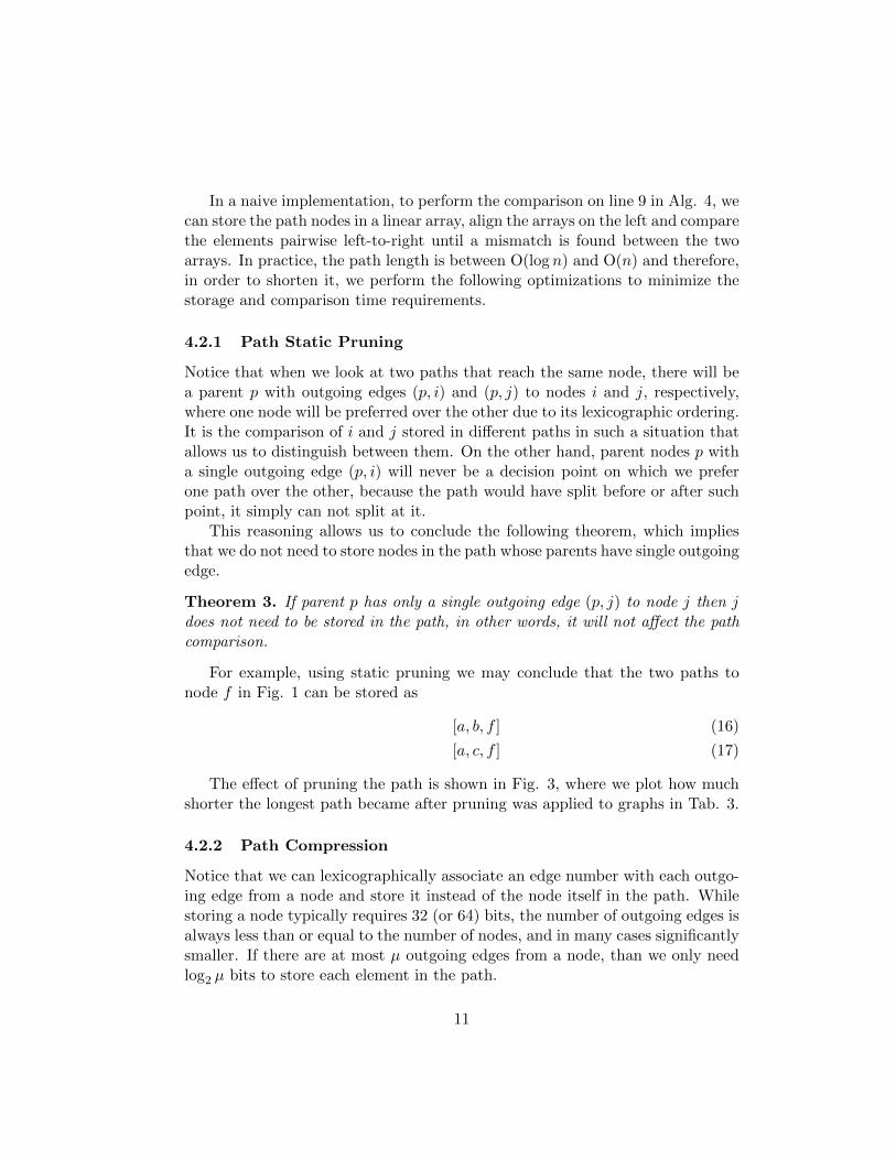
The effect of pruning the path is shown in Fig. 3, where we plot how muchshorter the longest path became after pruning was applied to graphs in Tab. 3.

4.2.2 Path Compression

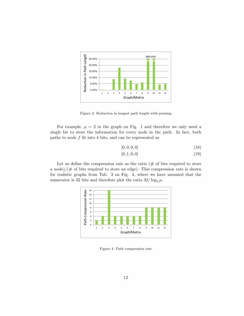
Notice that we can lexicographically associate an edge number with each outgo-ing edge from a node and store it instead of the node itself in the path. Whilestoring a node typically requires 32 (or 64) bits, the number of outgoing edges isalways less than or equal to the number of nodes, and in many cases significantlysmaller. If there are at most µ outgoing edges from a node, than we only needlog2 µ bits to store each element in the path.

11

0.00%

5.00%

10.00%

15.00%

20.00%

25.00%

1 2 3 4 5 6 7 8 9 10 11 12

ReductioninPathLength

Graph/Matrix

68%65%

Figure 3: Reduction in longest path length with pruning

For example, µ = 2 in the graph on Fig. 1 and therefore we only need asingle bit to store the information for every node in the path. In fact, bothpaths to node f fit into 4 bits, and can be represented as

[0, 0, 0, 0] (18)

[0, 1, 0, 0] (19)

Let us define the compression rate as the ratio (# of bits required to storea node)/(# of bits required to store an edge). This compression rate is shownfor realistic graphs from Tab. 3 on Fig. 4, where we have assumed that thenumerator is 32 bits and therefore plot the ratio 32/ log2 µ.

0

2

4

6

8

10

12

14

16

1 2 3 4 5 6 7 8 9 10 11 12

PathCom

pressionRate

Graph/Matrix

Figure 4: Path compression rate

12

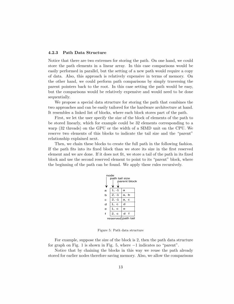
4.2.3 Path Data Structure

Notice that there are two extremes for storing the path. On one hand, we couldstore the path elements in a linear array. In this case comparisons would beeasily performed in parallel, but the setting of a new path would require a copyof data. Also, this approach is relatively expensive in terms of memory. Onthe other hand, we could perform path comparisons by simply traversing theparent pointers back to the root. In this case setting the path would be easy,but the comparisons would be relatively expensive and would need to be donesequentially.

We propose a special data structure for storing the path that combines thetwo approaches and can be easily tailored for the hardware architecture at hand.It resembles a linked list of blocks, where each block stores part of the path.

First, we let the user specify the size of the block of elements of the path tobe stored linearly, which for example could be 32 elements corresponding to awarp (32 threads) on the GPU or the width of a SIMD unit on the CPU. Wereserve two elements of this blocks to indicate the tail size and the “parent”relationship explained next.

Then, we chain these blocks to create the full path in the following fashion.If the path fits into its fixed block than we store its size in the first reservedelement and we are done. If it does not fit, we store a tail of the path in its fixedblock and use the second reserved element to point to its “parent” block, wherethe beginning of the path can be found. We apply these rules recursively.

1, -1 a

2, -1 a, b

2, -1 a, c

1, c d

1, c e

b

c

d

e

f

a

2, c d f

parent block

nodepath tail size

reserved path tail

Figure 5: Path data structure

For example, suppose the size of the block is 2, then the path data structurefor graph on Fig. 1 is shown in Fig. 5, where −1 indicates no “parent”.

Notice that by chaining the blocks in this way we reuse the path alreadystored for earlier nodes therefore saving memory. Also, we allow the comparisons

13

to be performed in parallel and enable early exit if the same “parent” is detectedfor both paths. Moreover, the cost of setting a new path is proportional to itstail size only.

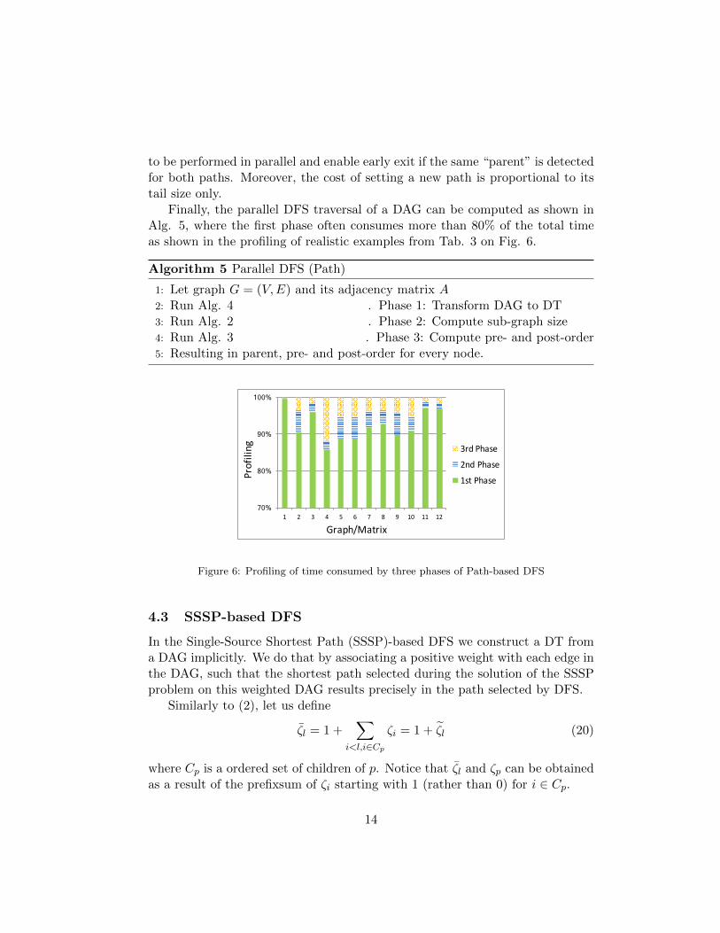
Finally, the parallel DFS traversal of a DAG can be computed as shown inAlg. 5, where the first phase often consumes more than 80% of the total timeas shown in the profiling of realistic examples from Tab. 3 on Fig. 6.

Algorithm 5 Parallel DFS (Path)

1: Let graph G = (V,E) and its adjacency matrix A2: Run Alg. 4 . Phase 1: Transform DAG to DT3: Run Alg. 2 . Phase 2: Compute sub-graph size4: Run Alg. 3 . Phase 3: Compute pre- and post-order5: Resulting in parent, pre- and post-order for every node.

70%

80%

90%

100%

1 2 3 4 5 6 7 8 9 10 11 12

Profiling

Graph/Matrix

3rdPhase

2ndPhase

1stPhase

Figure 6: Profiling of time consumed by three phases of Path-based DFS

4.3 SSSP-based DFS

In the Single-Source Shortest Path (SSSP)-based DFS we construct a DT froma DAG implicitly. We do that by associating a positive weight with each edge inthe DAG, such that the shortest path selected during the solution of the SSSPproblem on this weighted DAG results precisely in the path selected by DFS.

Similarly to (2), let us define

ζ̄l = 1 +∑

i<l,i∈Cp

ζi = 1 + ζ̃l (20)

where Cp is a ordered set of children of p. Notice that ζ̄l and ζp can be obtainedas a result of the prefixsum of ζi starting with 1 (rather than 0) for i ∈ Cp.

14

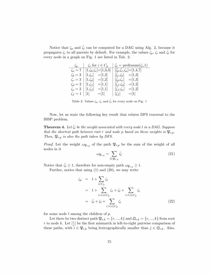
Notice that ζp and ζ̄l can be computed for a DAG using Alg. 2, because itpropagates ζi to all parents by default. For example, the values ζp, ζi and ζ̄l forevery node in a graph on Fig. 1 are listed in Tab. 2.

ζp ζi for i ∈ Cp ζ̄l = prefixsum(ζi,1)

ζa = 7 [1,ζb,ζc]=[1,3,3] [ζ̄b,ζ̄c,ζa]=[1,4,7]ζb = 3 [1,ζe] =[1,2] [ζ̄e,ζb] =[1,3]ζc = 3 [1,ζd] =[1,2] [ζ̄d,ζc] =[1,3]ζd = 2 [1,ζf ] =[1,1] [ζ̄f ,ζd] =[1,2]ζe = 2 [1,ζf ] =[1,1] [ζ̄f ,ζe] =[1,2]ζf = 1 [1] =[1] [ζf ] =[1]

Table 2: Values ζp, ζi and ζ̄l for every node on Fig. 1

Now, let us state the following key result that relates DFS traversal to theSSSP problem.

Theorem 4. Let ζ̄l be the weight associated with every node l in a DAG. Supposethat the shortest path between root r and node p based on these weights is Pr,p.Then, Pr,p is also the path taken by DFS.

Proof. Let the weight ωPr,p of the path Pr,p be the sum of the weight of allnodes in it

ωPr,p =∑l∈Pr,p

ζ̄l (21)

Notice that ζ̄l ≥ 1, therefore for non-empty path ωPr,p ≥ 1.Further, notice that using (1) and (20), we may write

ζp = 1 +∑i∈Cp

ζi

= 1 +∑

i<l,i∈Cp

ζi + ζl +∑

i>l,i∈Cp

ζi

= ζ̄l + ζl +∑

i>l,i∈Cp

ζi (22)

for some node l among the children of p.Let there be two distinct path Pr,k = {r, ..., k} and Qr,k = {r, ..., k} from root

r to node k. Let [ ij ] be the first mismatch in left-to-right pairwise comparison ofthese paths, with i ∈ Pr,k being lexicographically smaller than j ∈ Qr,k. Also,

15

ζi

ζj

ζk

p

i

k

j

Figure 7: Two distinct paths Pp,k and Qp,k

let their parent p belong to both paths Pr,k and Qr,k. Notice that node p canbe the root r, while i and j can be the node k, as shown in Fig 7.

Notice that based on the above assumptions paths are the same from rootr to node p, therefore we only need to consider the difference in path weightstarting at node p.

Then, notice that the weight of path Qp,k is given by

ωQp,k=

∑l∈Qp,k

ζ̄l

≥ ζ̄j ≥ ζ̄i + ζi (23)

≥ ζ̄i +∑z∈Pi,k

ζ̄z + ζk (24)

=∑

z∈Pp,k

ζ̄z + ζk (25)

>∑

z∈Pp,k

ζ̄z = ωPp,k(26)

where we have used (20) to obtain (23), applied (22) recursively, while droppingthe third term, to obtain (24), regrouped the terms to obtain (25) and tookadvantage of the fact that ζk ≥ 1 to obtain (26).

Thus, we have proven that the shortest path computed using weights ζ̄lindeed coincides with the lexicographically smallest DFS path.

4.3.1 SSSP Algorithms

There exist a variety of algorithms for computing SSSP [10, 11]. We propose aspecific approach for a DAG that traverses the graph top-down, from roots to

16

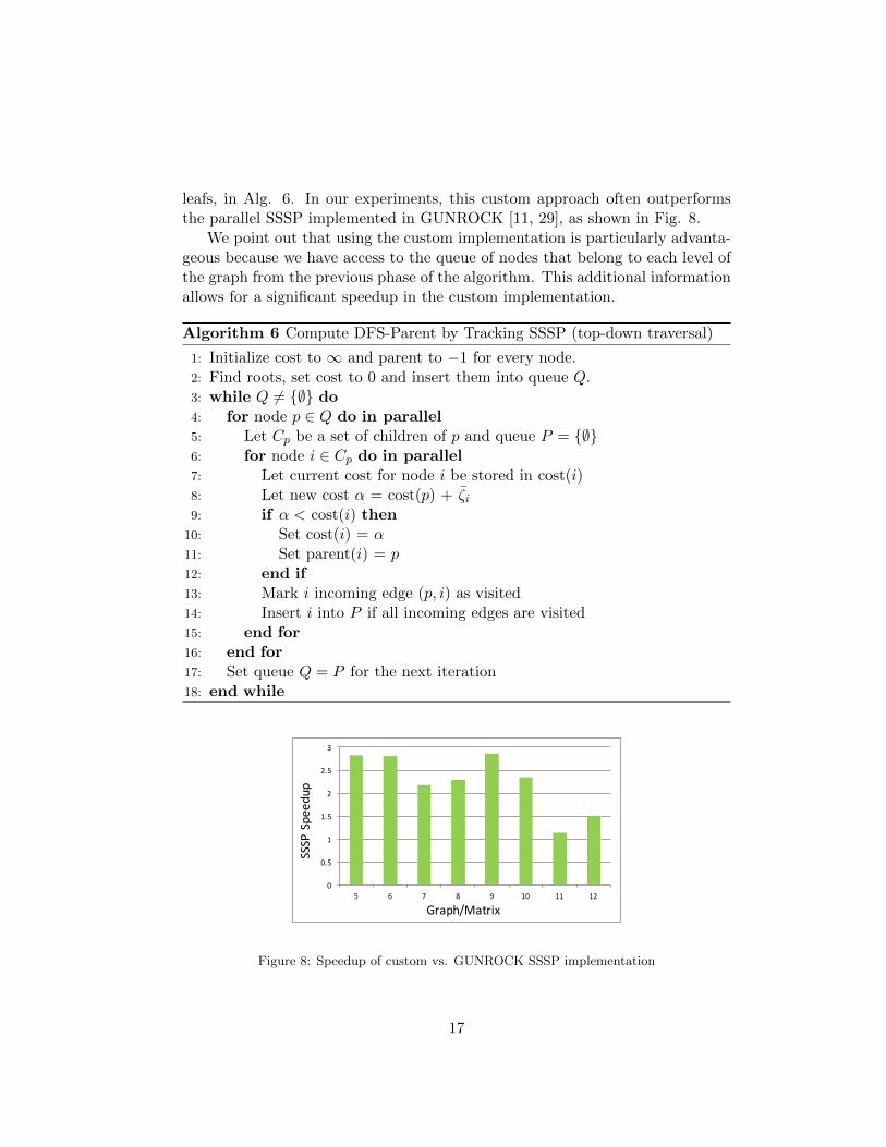
leafs, in Alg. 6. In our experiments, this custom approach often outperformsthe parallel SSSP implemented in GUNROCK [11, 29], as shown in Fig. 8.

We point out that using the custom implementation is particularly advanta-geous because we have access to the queue of nodes that belong to each level ofthe graph from the previous phase of the algorithm. This additional informationallows for a significant speedup in the custom implementation.

Algorithm 6 Compute DFS-Parent by Tracking SSSP (top-down traversal)

1: Initialize cost to ∞ and parent to −1 for every node.2: Find roots, set cost to 0 and insert them into queue Q.3: while Q 6= {∅} do4: for node p ∈ Q do in parallel5: Let Cp be a set of children of p and queue P = {∅}6: for node i ∈ Cp do in parallel7: Let current cost for node i be stored in cost(i)8: Let new cost α = cost(p) + ζ̄i9: if α < cost(i) then

10: Set cost(i) = α11: Set parent(i) = p12: end if13: Mark i incoming edge (p, i) as visited14: Insert i into P if all incoming edges are visited15: end for16: end for17: Set queue Q = P for the next iteration18: end while

0

0.5

1

1.5

2

2.5

3

5 6 7 8 9 10 11 12

SSSPSpeedup

Graph/Matrix

Figure 8: Speedup of custom vs. GUNROCK SSSP implementation

17

4.3.2 Pre- and Post-order

Once we have resolved the parent relationship, we could simply apply Alg. 2and 3 as done in phases 2 and 3 of Path-based approach to find the pre- andpost-order traversal of every node. However, in this section we will show that itis possible to completely avoid those traversals when pre-order only is needed.

Corollary 3. The ordering of nodes based on their path weight ωPr,p or pre-ordertime is the same.

Proof. First, notice that we can not directly use Thm. 1 to compute pre-orderand post-order of the nodes because the weights ζ̄l = 1 + ζ̃l have been computedfor a DAG and not a DT in this section.

However, notice that computed path weight ωPr,p imposes an ordering onthe nodes. For instance, nodes in the same path must come one after anotheraccording to their path weight. Also, nodes with the same parent are orderedlexicographically as shown in Thm. 4. If we apply this arguments recursively,we may conclude that the ordering based on path weight ωPr,p coincides withpre-order ordering.

On the other hand, notice that post-order can be expressed in terms of pre-order of a node as shown in the next Corollary. Therefore, if depth k is knownfor every node then we can completely avoid calling both Alg. 2 and 3 forcomputation of the pre- and post-order traversal. If the depth is not availablethen we can call Alg. 2 to obtain and use it for computing the post-order only.

Corollary 4. For a DT the post-order of node p can be expressed through itspre-order

post-order(p) = pre-order(p)− k + (ζp − 1) (27)

where k is the depth and ζp is the sub-graph size.

Proof. Follows directly from Thm. 1.

Finally, the SSSP-based parallel DFS traversal of a DAG can be computedas shown in Alg. 7. Notice that for graphs listed in Tab. 3 its first and secondphase often consume more than 80% of the total time as shown in Fig. 9.

Also, notice that the time consumed by the first and last phases using Alg.2 for DAG and DT traversals, respectively, is starkly different. This discrepancyis due mainly to two factors: (i) in the former case the graph has many moreedges, and (ii) in the latter case a node may be scheduled into the queue earlierbecause its dependencies, have been already satisfied. It is important to keepthis distinction in mind when analysing the algorithm.

18

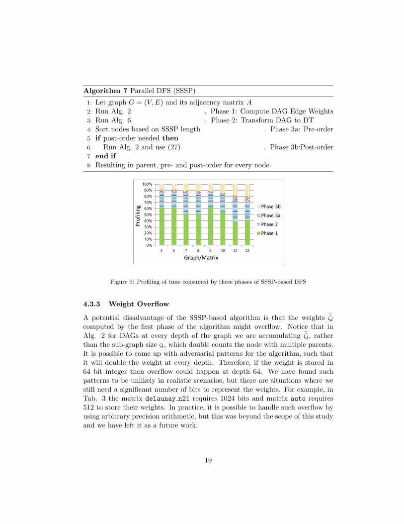
Algorithm 7 Parallel DFS (SSSP)

1: Let graph G = (V,E) and its adjacency matrix A2: Run Alg. 2 . Phase 1: Compute DAG Edge Weights3: Run Alg. 6 . Phase 2: Transform DAG to DT4: Sort nodes based on SSSP length . Phase 3a: Pre-order5: if post-order needed then6: Run Alg. 2 and use (27) . Phase 3b:Post-order7: end if8: Resulting in parent, pre- and post-order for every node.

0% 10% 20% 30% 40% 50% 60% 70% 80% 90%

100%

5 6 7 8 9 10 11 12

Profiling

Graph/Matrix

Phase3b

Phase3a

Phase2

Phase1

Figure 9: Profiling of time consumed by three phases of SSSP-based DFS

4.3.3 Weight Overflow

A potential disadvantage of the SSSP-based algorithm is that the weights ζ̄lcomputed by the first phase of the algorithm might overflow. Notice that inAlg. 2 for DAGs at every depth of the graph we are accumulating ζ̄l, ratherthan the sub-graph size ςl, which double counts the node with multiple parents.It is possible to come up with adversarial patterns for the algorithm, such thatit will double the weight at every depth. Therefore, if the weight is stored in64 bit integer then overflow could happen at depth 64. We have found suchpatterns to be unlikely in realistic scenarios, but there are situations where westill need a significant number of bits to represent the weights. For example, inTab. 3 the matrix delaunay n21 requires 1024 bits and matrix auto requires512 to store their weights. In practice, it is possible to handle such overflow byusing arbitrary precision arithmetic, but this was beyond the scope of this studyand we have left it as a future work.

19

4.4 Complexity Analysis

Let n and m be the number of nodes and edges in a DAG. Also, let us assumea standard theoretical PRAM (CREW) model for the formal analysis [16].

Definition 4. Let ki be the number of elements inserted into the queue at iter-ation i and k = maxi ki in Alg. 2-4 and 6.

Definition 5. Let di denote the degree of node i and d = maxi di denote themaximum degree in a DAG.

Definition 6. Let δi denote the minimum depth1 of node i and δ = maxi δidenote the diameter in a DAG.

Definition 7. Let ηi denote the maximum depth2 of node i and η = maxi ηidenote the length of the longest path in a DAG.

Lemma 2. The parallel prefixsum of n numbers, can be computed in O(log n)steps. Also, the algorithm performs O(n) work.

Proof. Please refer to [8].

Lemma 3. The parallel (comparison-based) sort of n numbers, can be computedin O(log n) steps. The algorithm performs O(n log n) work.

Proof. Please refer to [9].

Lemma 4. Let n = min(n1, n2) then identifying the first left-to-right pair ofdigits that is different in two sequences of n1 and n2 numbers can be performedin O(log n) steps. Also, the algorithm performs O(n) work.

Proof. Let the sequences be aligned on the leftmost digit and let processor i beassigned the i-th pair of numbers. Let it compute either index i if its pair ofdigits is different or∞ otherwise, which can be done in O(1). Then, we can finda minimum of the results using a binary tree-like reduction implemented usinga prefixsum, see Lemma 2.

Lemma 5. The queue can be implemented such that parallel insertion and ex-traction of n numbers, can be performed in O(log n) and O(1) steps, respectively.Also, the algorithm performs O(n) work.

1The length of the shortest path from the root to a node.2The length of the longest path from the root to a node.

20

Proof. Suppose that we store the queue data in linear array with the start andend indices. Also, suppose that at each iteration we extract all data elementsbetween the start and end indices and we insert new data elements immediatelyafter the end index. Then, we adjust the start and end indices to point to thenewly inserted data for the next iteration and repeat the process.

In this scenario we can extract all data elements in parallel in O(1) steps. Inorder to insert the elements in parallel without write conflicts, we may chooseto assign a unique write index to each processor to indicate a particular locationin the array where the element can be written safely. Notice that such a writeindex can be computed using a prefixsum, see Lemma 2.

Notice that for DT η = δ, while for a DAG η ≥ δ. Also, notice that k, d, δ, η ≤n for a DAG. Let us now state the complexity of each phase of parallel DFS.

Theorem 5. Alg. 2 takes O(η(log d+log k)) steps and performs O(m+n) totalwork to traverse a DAG. The number of processors t ≤ m + n actively doingwork varies at each step of the algorithm.

Proof. The Alg. 2 performs η while loop iterations because we enqueue a nodeonce all its edges are visited.

In each iteration, notice that we can access ζp,i on line 7 in O(1). Also, theparallel prefixsum performed on line 14 takes no more than O(log d), see Lemma2. We might need to perform multiple of these prefixsums at once, but we willnever be using more than m edges. Therefore, we need at most O(m) processorsfor it. Also, at each iteration we might need to insert k ≤ n elements into aqueue on line 9, which can be done in O(log k), see Lemma 5.

Notice that work performed for each iteration is O(di+ki). Since m =∑

i diand n =

∑i ki, the total work performed is O(m+ n).

Theorem 6. Alg. 3 takes O(η log k) steps and performs O(n) total work totraverse a DAG. The number of processors t ≤ n actively doing work varies ateach step of the algorithm.

Proof. The Alg. 3 performs O(η) while loop iterations, with each iterationrequiring O(1) operations. However, at each iteration we might need to insertk ≤ n elements into a queue on line 12, which can be done in O(log k), seeLemma 5. The work performed for each iteration is O(ki). Since n =

∑i ki, the

total work performed is O(n).

Theorem 7. Alg. 4 takes O(η(log η + log k)) steps and performs O(ηm + n)total work to traverse a DAG. The number of processors t ≤ ηd + n activelydoing work varies at each step of the algorithm.

21

Proof. The Alg. 4 performs O(η) while loop iterations.Notice that per iteration the most time consuming part of the algorithm

involves path comparison Pr,i ≤ Qr,i on line 9. It can be performed in O(log η),see Lemma 4. We might need to perform multiple path comparisons at once,therefore we might need O(ηd) processors. The work performed for each path(sequence) comparison is O(η). There are no more than m =

∑i di sequences

to compare, therefore we perform O(ηm) total work for it.The path exchange Qr,i = Pr,i on line 10 can be performed in O(1), be-

cause we only replace the (fixed size) path tail, using previously discussed datastructure, see Fig. 5.

Also, at each iteration we might need to insert k ≤ n elements into a queueon line 14, which can be done in O(log k), see Lemma 5. The work performedfor this operation at each iteration is O(ki). Since n =

∑i ki, the total work

performed for this operation is O(n).

Theorem 8. Alg. 6 takes O(η log k) steps and performs O(n) total work totraverse a DAG. The number of processors t ≤ n actively doing work varies ateach step of the algorithm.

Proof. Follows proof of Thm. 6.

The complexity of sequential DFS is O(m+n). The complexity of the novelparallel DFS variants is stated below.

Corollary 5. The Path-based DFS in Alg. 5 takes O(η(log d + log k + log η))steps and performs O(m+ n+ ηm) total work to traverse a DAG. The numberof processors t ≤ m + n + ηd actively doing work varies at each step of thealgorithm.

Notice that in practice ηm → m because the data structure for storing thepath detects the same “parent” block during comparisons, which often implicitlyeliminates additional work, see Fig. 5. Also, recall that d, k, η ≤ n in a DAGand therefore the Path-based algorithm takes no more than O(η log n) steps andperforms O(m+ n) total work.

Corollary 6. The SSSP-based DFS in Alg. 7 takes O(η(log d + log k)) stepsand performs O(m+ n+ n log n) total work to traverse a DAG. The number ofprocessors t ≤ m+ n actively doing work varies at each step of the algorithm.

Notice that the work complexity of parallel sort can be improved by usingnon-comparison based algorithms, such as radix sort, in which case n log n→ n.Since d, k ≤ n in a DAG, we may conclude that SSSP-based algorithm takes nomore than O(η log n) steps and performs O(m+ n) total work.

22

Moreover, real-world graphs are often sparse with the number of edges m =γn where γ is some small constant. Consequently, in practice the total workperformed for both Path- and SSSP-based parallel DFS is often O(n).

Finally, notice that while the parallel complexity of BFS is related to diam-eter δ [19], we have shown that the parallel complexity of lexicographic DFS isrelated to the length of the longest path η in a DAG.

5 Experiments

We study the performance of the DFS algorithm on a variety of graphs fromthe UFSMC and DIMACS collections [12] shown in Tab. 3. These graphs areselected from different applications and have very different node degree, longestpath length and other characteristics, which allows us to make a more substantiveanalysis of the performance. When necessary we create DAGs based on thesegeneral graphs by dropping the back edges, in other words, only considering thelower triangular part of the adjacency matrix.

# Graph n m Application

1. coPapersDBLP 540487 15251812 Citations

2. auto 448696 3350678 Numeric. Sim.3. hugebubbles-000 18318144 30144175 Numeric. Sim.

4. delaunay n24 16777217 52556391 Random Tri.

5. il2010 451555 1166978 Census Data6. fl2010 484482 1270757 Census Data7. ca2010 710146 1880571 Census Data8. tx2010 914232 2403504 Census Data

9. great-britain osm 7733823 8523976 Road Network10. germany osm 11548846 12793527 Road Network11. road central 14081817 21414269 Road Network12. road usa 23947348 35246600 Road Network

Table 3: Sample DIMACS graphs/adjacency matrices

The experiments are performed on the workstation with Intel Core i7-3930K@3.2GHz CPU and Nvidia Pascal TitanX GPU with Ubuntu 14.04 LTS OS andCUDA Toolkit 8.0. We use standard sequential implementation of the DFS [10],written in C programming language and compiled with gcc compiler and -O3optimization flags. We compare it against the Path- and SSSP-based parallelDFS implementations written in CUDA and compiled with nvcc compiler with-O3 optimization flags.

23

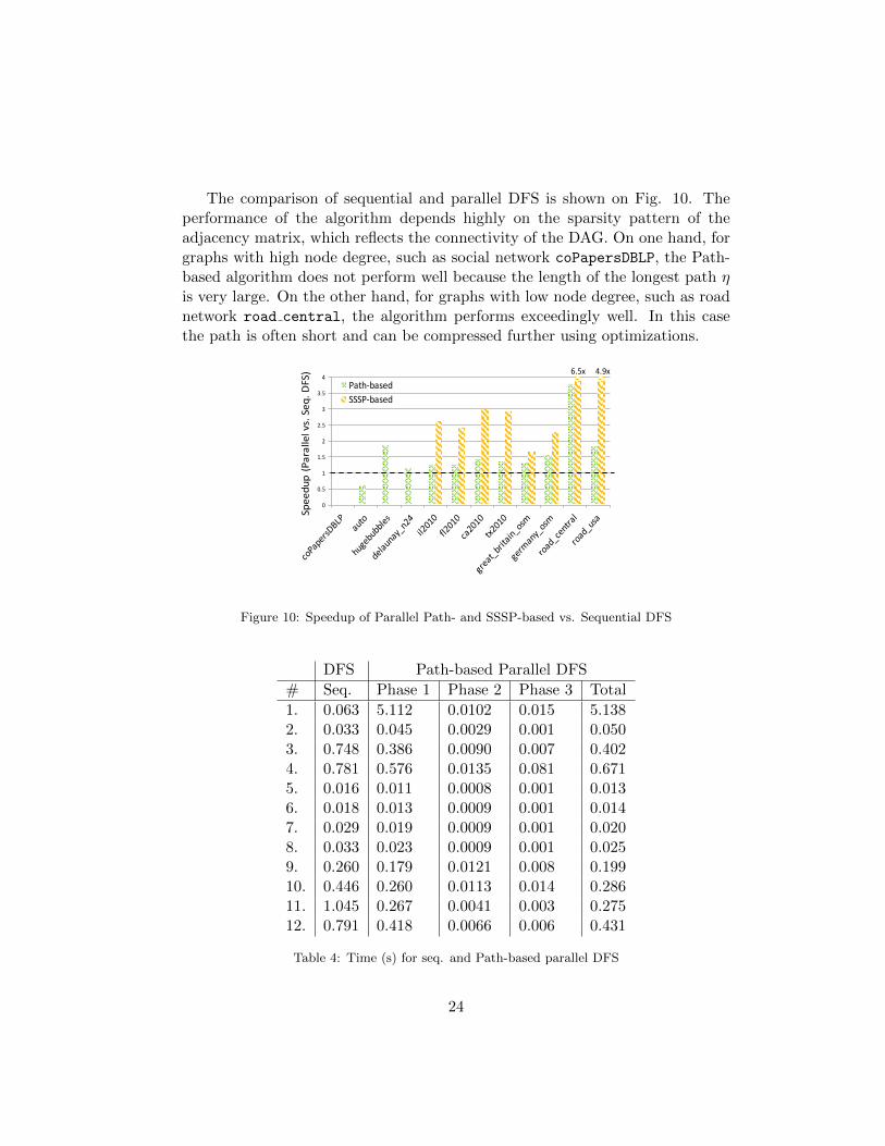
The comparison of sequential and parallel DFS is shown on Fig. 10. Theperformance of the algorithm depends highly on the sparsity pattern of theadjacency matrix, which reflects the connectivity of the DAG. On one hand, forgraphs with high node degree, such as social network coPapersDBLP, the Path-based algorithm does not perform well because the length of the longest path ηis very large. On the other hand, for graphs with low node degree, such as roadnetwork road central, the algorithm performs exceedingly well. In this casethe path is often short and can be compressed further using optimizations.

0

0.5

1

1.5

2

2.5

3

3.5

4

Speedup(Parallelvs.Seq.D

FS)

Path-basedSSSP-based

6.5x 4.9x

Figure 10: Speedup of Parallel Path- and SSSP-based vs. Sequential DFS

DFS Path-based Parallel DFS

# Seq. Phase 1 Phase 2 Phase 3 Total

1. 0.063 5.112 0.0102 0.015 5.1382. 0.033 0.045 0.0029 0.001 0.0503. 0.748 0.386 0.0090 0.007 0.4024. 0.781 0.576 0.0135 0.081 0.6715. 0.016 0.011 0.0008 0.001 0.0136. 0.018 0.013 0.0009 0.001 0.0147. 0.029 0.019 0.0009 0.001 0.0208. 0.033 0.023 0.0009 0.001 0.0259. 0.260 0.179 0.0121 0.008 0.19910. 0.446 0.260 0.0113 0.014 0.28611. 1.045 0.267 0.0041 0.003 0.27512. 0.791 0.418 0.0066 0.006 0.431

Table 4: Time (s) for seq. and Path-based parallel DFS

24

DFS SSSP-based Parallel DFS

# Seq. Phase 1 Phase 2 Phase 3a Phase 3b Total

5. 0.016 0.004 0.001 0.000 0.001 0.0066. 0.018 0.005 0.002 0.000 0.001 0.0077. 0.029 0.005 0.003 0.001 0.001 0.0098. 0.033 0.006 0.004 0.001 0.001 0.0119. 0.260 0.098 0.034 0.005 0.018 0.15410. 0.446 0.115 0.053 0.007 0.028 0.20311 1.045 0.061 0.058 0.010 0.030 0.15812. 0.791 0.066 0.047 0.015 0.032 0.160

Table 5: Time (s) for seq. and SSSP-based parallel DFS

Also, notice that when there is no weight overflow the SSSP-based DFSattains higher performance than Path-based DFS. In a way it exchanges thepath comparisons for weight additions, which are more computationally efficient.However, in practice the algorithms are complementary. The former works bestwhen there is limited nesting of the sub-graphs (so that the computation of theweight does not overflow and require special handling), while the latter worksbest when the path to every node is relatively short (so that path comparisoncan be done quickly).

Finally, the detailed results are stated in Tab. 4 and 5, where results forwhich 32 bit integer weights overflowed are not present.

6 Conclusion

In this paper we have developed a work-efficient parallel DFS algorithm thatfinds parent, pre- and post-order relationship for every node in a DAG. Thealgorithm performs up to three BFS-like traversals of the DAG and has Path-and SSSP-based complementary variations. We have proven that both variationsof the algorithm obtain correct results and performed their runtime and workanalysis.

The performance of the parallel algorithm depends highly on the connectiv-ity of the DAG, in other words, the sparsity pattern of the adjacency matrix.In our experiments its parallel implementation performed particularly well onDAGs with low node degree, such as census and road networks, where it hasoutperformed by up to 6× the sequential DFS.

25

7 Acknowledgments

The authors would like to thank Isaac Gelado for providing a locking libraryon the GPU that was used during path comparisons and exchanges, as well asSteven Dalton, Alex Fit-Florea, Duane Merrill and Sean Treichler for insightfulcomments and suggestions.

References

[1] U. A. Acar, A. Chargueraud, and M. Rainey. A work-efficient algorithm forparallel unordered depth-first search. Proc. Supercomputing, 67, 2015.

[2] A. Aggarwal and R. J. Anderson. A random NC algorithm depth firstsearch. Proc. ACM Symp. Theory of Computing, pages 325–334, 1987.

[3] A. Aggarwal, R. J. Anderson, and M. Y. Kao. Parallel depth-first search indirected graphs. Proc. ACM Symp. Theory of Computing, pages 297–308,1989.

[4] A. Aggarwal, R. J. Anderson, and M. Y. Kao. Parallel depth-first search ingeneral directed graphs. SIAM Journal on Computing, 19:397–409, 1990.

[5] S. Alstrup, C. Gavoille, H. Kaplan, and T. Rauhe. Nearest common ances-tors: A survey and a new algorithm for a distributed environment. Theoryof Computing Systems, 37:441–456, 2004.

[6] S. Arora and B. Barak. Computational Complexity: A Modern Approach.Cambridge University Press, New York, NY, 2009.

[7] M. Atallah and U. Vishkin. Finding Euler tours in parallel. Journal ofComputer and System Sciences, 29:330–337, 1984.

[8] G. E. Blelloch. Prefix sums and their applications. Carnegie Mellon Uni-versity, CS-TR-190, 1990.

[9] R. Cole. Parallel merge sort. SIAM Journal on Computing, 17:770–785,1988.

[10] T. H. Cormen, C. E. Leiserson, R. L. Rivest, and C. Stein. Introduction toAlgorithms. The MIT Press, Camb., MA, 2001.

[11] A. Davidson, S. Baxter, M. Garland, and J. D. Owens. Work-efficient paral-lel GPU methods for single-source shortest paths. Proc. IEEE InternationalSymp. Parallel and Distributed Processing, pages 349–359, 2014.

26

[12] T. Davis. The University of Florida Sparse Matrix Collection.http://www.cise.ufl.edu/research/sparse/matrices/.

[13] R. K. Ghosh and G. P. Bhattacharjee. A parallel search algorithm fordirected acyclic graphs. BIT, 24:134–150, 1984.

[14] T. Hagerup. Planar depth-first search in O(log n) parallel time. SIAMJournal on Computing, 19:678–704, 1990.

[15] J. Hopcroft and R. E. Tarjan. Efficient planarity testing. Journal ACM.

[16] J. JaJa. An Introduction to Parallel Algorithms. Addison-Wesley, 1992.

[17] E. Korach and Z. Ostfeld. Recognition of DFS trees: Sequential and parallelalgorithms with refined verifications. Discrete Mathematics, 114:305–327,1993.

[18] J. Ma, K. Iwama, T. Takaoka, and Q. Gu. Efficient parallel and distributedtopological sort algorithms. Proc. International Symp. Parallel Algorithmsand Architecture Synthesis, page 378, 1997.

[19] D. Merrill, M. Garland, and A. Grimshaw. Scalable GPU graph traversal.Proc. ACM SIGPLAN Symp. Principles and Practice of Parallel Program-ming, 2012.

[20] C. Peng, B. Wang, and J. Wang. Recognizing unordered depth-first treesof an undirected graph in parallel. IEEE Trans. Parallel and DistributedSystems, 11:559–570, 2000.

[21] J. H. Reif. Depth-first search is inherently sequential. Information Process-ing Letters, 20:229–234, 1985.

[22] C. A. Schevon and J. S. Vitter. A parallel algorithm for recognizing un-ordered depth-first search. Information Processing Letters, 28:105–110,1988.

[23] G. Shannon. A linear-processor algorithm for depth-first search in planargraphs. Purdue University, CS-TR-737, 1988.

[24] J. R. Smith. Parallel algorithms for depth-first searches i. planar graphs.SIAM Journal on Computing, 15:814–830, 1986.

[25] R. E. Tarjan. Depth-first search and linear graph algorithms. SIAM Journalon Computing, 1:146–160, 1972.

27

[26] R. E. Tarjan and U. Vishkin. Finding biconnected components and com-puting tree functions in logarithmic parallel time. Foundations of ComputerScience, pages 12–20, 1984.

[27] Y. H. Tsin. Finding lowest common ancestors in parallel. IEEE Transac-tions on Computers, 35:764–769, 1986.

[28] U. Vishkin and R. E. Tarjan. An efficient parallel biconnectivity algorithm.SIAM Journal on Computing, 14:862–874, 1985.

[29] Y. Wang, A. Davidson, Y. Pan, Y. Wu, A. Riffel, and J. D. Owens. Gunrock:A high-performance graph processing library on the GPU. Proc. ACMSIGPLAN Symp. Principles and Practice of Parallel Programming, 2016.

[30] Y. Zhang. A note on parallel depth first search. BIT, 26:195–198, 1986.

28