Parallel FFT Libraries

Evangelos Brachos

August 19, 2011

MSc in High Performance Computing

The University of Edinburgh

Year of Presentation: 2011

Abstract

The focus of this project is the area of the fast Fourier transform (FFT) libraries(FFTW 3.3, P3DFFT 2.4 and 2DECOMP&FFT 1.1.319). During this project we bench-mark the libraries on Hector phase 2b supercomputer. The main goal of this project isto examine the performance of the libraries which are built on the top of the FFTW’slatest version and compare their results with the FFTW itself. Moreover, the abilityof the P3DFFT and the 2DECOMP&FFT to implement the 2D decomposition, let usexperiment with the scaling of these libraries in thousands of cores. The findings fromthis experiment provide evidence of the FFTW library’s excellent scaling by using the1D decomposition and the ability of the other two libraries to minimise the time re-quired for the Fourier transform computation, by using the 2D decomposition. Themain conclusions drawn from this study were the ability of the P3DFFT and the 2DE-COMP&FFT libraries to scale up to thousands of cores and the affects of the GeminiInterconnect on their performance.

Contents

1 Introduction 1

2 Background Theory 42.1 Fourier Analysis . . . . . . . . . . . . . . . . . . . . . . . . . . . . . . 42.2 Fourier Transform . . . . . . . . . . . . . . . . . . . . . . . . . . . . . 42.3 Fourier Series . . . . . . . . . . . . . . . . . . . . . . . . . . . . . . . 5

2.3.1 Discrete Fourier Transform (DFT) . . . . . . . . . . . . . . . . 52.3.2 Fast Fourier Transform (FFT) . . . . . . . . . . . . . . . . . . 6

2.4 Parallel FFT in Three Dimensions . . . . . . . . . . . . . . . . . . . . 62.4.1 Parallelisation of the 3D FFT . . . . . . . . . . . . . . . . . . . 72.4.2 1D Decomposition . . . . . . . . . . . . . . . . . . . . . . . . 72.4.3 2D Decomposition . . . . . . . . . . . . . . . . . . . . . . . . 8

2.5 FFT Libraries . . . . . . . . . . . . . . . . . . . . . . . . . . . . . . . 92.5.1 Parallel FFT Libraries . . . . . . . . . . . . . . . . . . . . . . 102.5.2 FFTW 3.3 . . . . . . . . . . . . . . . . . . . . . . . . . . . . . 102.5.3 P3DFFT . . . . . . . . . . . . . . . . . . . . . . . . . . . . . 122.5.4 2DECOMP&FFT . . . . . . . . . . . . . . . . . . . . . . . . . 142.5.5 Features Comparison . . . . . . . . . . . . . . . . . . . . . . . 15

3 Design and Implementation 163.1 Design . . . . . . . . . . . . . . . . . . . . . . . . . . . . . . . . . . . 163.2 Implementation . . . . . . . . . . . . . . . . . . . . . . . . . . . . . . 17

3.2.1 Programming Languages . . . . . . . . . . . . . . . . . . . . . 183.2.2 Compilation . . . . . . . . . . . . . . . . . . . . . . . . . . . 183.2.3 FFT Libraries Installation . . . . . . . . . . . . . . . . . . . . 183.2.4 Test Data . . . . . . . . . . . . . . . . . . . . . . . . . . . . . 203.2.5 Test Programs . . . . . . . . . . . . . . . . . . . . . . . . . . . 203.2.6 Scripts . . . . . . . . . . . . . . . . . . . . . . . . . . . . . . 22

4 Experimental Design 244.1 HPC Systems Architecture . . . . . . . . . . . . . . . . . . . . . . . . 24

4.1.1 Hardware . . . . . . . . . . . . . . . . . . . . . . . . . . . . . 244.1.2 Interconnection Network . . . . . . . . . . . . . . . . . . . . . 264.1.3 Compiler . . . . . . . . . . . . . . . . . . . . . . . . . . . . . 26

4.2 Experiments Setup . . . . . . . . . . . . . . . . . . . . . . . . . . . . 27

i

4.2.1 Testing Different Decompositions . . . . . . . . . . . . . . . . 274.2.2 Reporting . . . . . . . . . . . . . . . . . . . . . . . . . . . . . 28

5 Results and Performance Analysis 305.1 Slabs and Pencils on Hector . . . . . . . . . . . . . . . . . . . . . . . 30

5.1.1 1D Decomposition (Slab) . . . . . . . . . . . . . . . . . . . . 305.1.2 1D Decomposition Performance Analysis . . . . . . . . . . . . 355.1.3 2D Decomposition (Rods or Pencils) . . . . . . . . . . . . . . 385.1.4 Processors Grid Selection . . . . . . . . . . . . . . . . . . . . 395.1.5 2D Decomposition Performance . . . . . . . . . . . . . . . . . 415.1.6 2D Decomposition Performance Analysis . . . . . . . . . . . . 44

5.2 Slabs versus Pencils on Hector . . . . . . . . . . . . . . . . . . . . . . 45

6 Conclusions & Discussions 506.1 Conclusions . . . . . . . . . . . . . . . . . . . . . . . . . . . . . . . . 506.2 Discussions . . . . . . . . . . . . . . . . . . . . . . . . . . . . . . . . 516.3 Future Work . . . . . . . . . . . . . . . . . . . . . . . . . . . . . . . . 52

A Results 54A.1 1D and 2D decomposition results . . . . . . . . . . . . . . . . . . . . . 54

ii

List of Tables

2.1 Stages During the 2D Decomposition . . . . . . . . . . . . . . . . . . 82.2 FFTW, P3DFFT and 2DECOMP&FFT features. . . . . . . . . . . . . . 15

4.1 Hector hardware specifications. . . . . . . . . . . . . . . . . . . . . . . 254.2 Gemini Interconnect on Hector phase 2b. . . . . . . . . . . . . . . . . 264.3 1D decomposition test parameters . . . . . . . . . . . . . . . . . . . . 274.4 1D decomposition test parameters . . . . . . . . . . . . . . . . . . . . 28

5.1 SLAB: 2563, 1 core per node, time and speedup. . . . . . . . . . . . . . 315.2 SLAB: 2563, 16 cores per node, time and speedup. . . . . . . . . . . . 325.3 SLAB: 1283, one core per node, time and speedup. . . . . . . . . . . . 335.4 SLAB: 1283, 16 cores per node, time and speedup. . . . . . . . . . . . 345.5 SLAB: 2563, FFTW OpenMP version versus MPI in one node. . . . . . 355.6 2563: 1D & 2D decomposition results. . . . . . . . . . . . . . . . . . . 465.7 1283: 1D & 2D decomposition results. . . . . . . . . . . . . . . . . . . 485.8 1283: 2D decomposition results for 512 Hector’s nodes. . . . . . . . . . 48

A.1 PENCIL: 2563, 16 cores per node, time and speedup. . . . . . . . . . . 56A.2 PENCIL: 2563, one core per node, time and speedup. . . . . . . . . . . 57A.3 PENCIL: 1283, one core per node, time and speedup. . . . . . . . . . . 57A.4 PENCIL: 1283, 16 cores per node, time and speedup. . . . . . . . . . . 58

iii

List of Figures

2.1 2D decomposition of 3D FFT. . . . . . . . . . . . . . . . . . . . . . . 82.2 2D decomposition of the P3DFFT. . . . . . . . . . . . . . . . . . . . . 13

3.1 FFT benchmarking methodology . . . . . . . . . . . . . . . . . . . . . 17

5.1 SLAB: Speedup using 2563 3D FFT with one core per node. . . . . . . 315.2 SLAB: Speedup using 2563 3D FFT with 16 cores per node . . . . . . . 325.3 SLAB: Speedup using 1283 3D FFT 1 core per node . . . . . . . . . . . 345.4 Libraries performance using 1283 3D FFT 16 cores per node. . . . . . . 355.5 SLAB: Speedup using 1283 3D FFT 16 cores per node. . . . . . . . . . 365.6 Libraries performance using 2563 3D array, 1024 total cores. . . . . . . 405.7 PENCIL: Speedup using 2563 3D FFT 1 and 16 cores per node. . . . . 425.8 PENCIL: Speedup using 1283 3D FFT 1 and 16 cores per node. . . . . 435.9 Speedup using 2563 3D FFT 1-16 cores per node. . . . . . . . . . . . . 475.10 Speedup using 1283 3D FFT, 1 and 16 cores per node. . . . . . . . . . . 49

A.1 SLAB: Libraries performance using 2563 3D FFT with 1 core per node. 54A.2 SLAB: Libraries performance using 2563 3D FFT, 16 cores per node. . 55A.3 SLAB: Libraries performance using 1283 3D FFT, one core per node. . 55A.4 OpenMP performance versus the MPI implementations up to 16 cores

- 2563 3D FFT. . . . . . . . . . . . . . . . . . . . . . . . . . . . . . . 56A.5 PENCIL: Libraries performance using 1283 3D FFT, one core per node. 58A.6 PENCIL: Libraries performance using 1283 3D FFT, 16 cores per node. 59A.7 PENCIL: Libraries performance using 2563 3D FFT, one core per node. 59A.8 PENCIL: Libraries performance using 2563 3D FFT, 16 cores per node. 60A.9 Libraries performance using 2563 3D FFT, 512 total cores. . . . . . . . 60

iv

Acknowledgements

I would like to thank my supervisor Dr. Stephen Booth for the help and guidance hehas given me. I would also like to thank Dr. Ning Li for all his assistance and thevaluable resources he has sent to me. Finally, I would like to thank my parents for theirencouragement.

Chapter 1

Introduction

Introduction

Fast Fourier transform (FFT) libraries are used by many researchers in many scien-tific areas and industries. The Fast Fourier Transform has been one of the most popularnumerical methods which is applied in almost every field of science such as oil ex-ploration, signal processing, Monte Carlo simulations, molecular dynamics and manyothers.

The computation of the fast Fourier transform is a very demanding operation and re-quires a lot of time to complete depending on the size of the problem and on many otherissues which will be presented on the following pages of this report. The fast Fouriertransform computation can be executed much faster using parallel processing, espe-cially nowadays, as many supercomputing facilities are available to scientists across theworld. Furthermore, the multicore desktop computers offer the capability of parallelprocessing.

Every word in the result of an FFT depends on every input word. A parallel imple-mentation of the FFT therefore requires significant number of communications.

The scientific computation of the fast Fourier transform algorithm could be imple-mented by using one of the many available FFT libraries which, in turn, make use ofdifferent implementations of the FFT.

In order to improve the performance of the fast Fourier transform computation it isvery important to carefully choose the right FFT library. Sometimes the correct choiceof a library seems to improve the program performance and reduce the computationtime. However, that choice depends on the hardware architecture, on the nature of the

1

problem (type of data), on the implementation (sequential or parallel) and on the budget(some libraries are open source while some other are commercial).

Most of the FFT libraries offer parallel computation support using different program-ming models such POSIX [1], MPI [2], OpenMP [3], CUDA [4] and others (either CPUor GPU programming models). This capability decreases the computational time of theFourier transform.

The performance of the FFT parallel computation poses a large number of issues re-garding the scalability and some other aspects which sometimes become a bottleneck,either physical (interconnection network) or of a design nature (demanding communi-cation of the fast Fourier transform). All of these issues, prevent the scientific programswhich use FFT to scale up to a large number of processors.

Thus, it is very important to know the performance of different FFT libraries in theparallel FFT computation. Such knowledge could facilitate the scientists to know thescaling of their programs which compute the fast Fourier transform of a 3D mesh withcertain dimensions by using one of the available FFT libraries. This will help reducethe financial costs required for deployment of resources in order to compute the 3D FFTin parallel.

On this project an extended benchmarking procedure implemented comparing the testprograms performance which compute the 3D FFT by using the FFTW 3.3 [5] library,the P3DFFT [6] 2.4 and 2DECOMP&FFT [7] 1.1.319 which are built on the top of theFFTW 3.3. The performance analysis was conducted on Hector [8] phase 2b.

Outline

In the following pages an analytical description of the FFT libraries, used for thisproject, is made along with the implemented test programs and benchmarking proce-dure.

In particular the report is divided into six chapters:

Chapter 1 In this chapter we introduce briefly the fast Fourier transform usage and theexistence of the FFT libraries.

Chapter 2 In this chapter we presented all the mathematical background of the prob-lem and the FFT libraries features.

2

Chapter 3 This chapter is referring to the design and analysis methodology which im-plemented by such projects and the steps we made to implement this project.

Chapter 4 This chapter is referring to the HPC systems architectures by analysing thesupercomputer’s software and hardware. There is also a discussion about the testswe made along with the combinations of the arguments we used.

Chapter 5 We made an extended presentation of the obtained results. After the resultspresentation of each decomposition there is an analysis for the particular decom-position results. At the end of this chapter there is a comparison between the twodecompositions approaches.

Chapter 6 In this chapter we interpreted the results and we made conclusions about thedifferent libraries and the different decompositions. Then follows a section wherewe presented some suggestions in order to give some directions about furtherimprovement of this project in the future.

Appendix At the end of the report we presented some of the most important obtainedresults by using tables and graphs.

3

Chapter 2

Background Theory

2.1 Fourier Analysis

Joseph Fourier proved that any continuous function could be produced as an infinitesum of simpler trigonometric functions.

2.2 Fourier Transform

Fourier transform is part of Fourier analysis and it is a general form for a continuousand aperiodic time signal f(k).

The Fourier transform is a mathematical method that decomposes a signal into theseries of frequencies that compose the time series.Forward Fourier Transform:

F (k) =

� ∞

−∞f(x)e−2πikx

dx, ∀k�R

Inverse Fourier Transform:

f(x) =

� ∞

−∞F (k)e2πikxdk, ∀k�R

The basis of Fourier transform is the Euler’s formula eiϕ = cosϕ + isinϕ. A complex

exponential is a complex number where the real and the imaginary parts are sinusoids.

For two dimensions the Fourier transform becomes:

F (x, y) =

� ∞

−∞

� ∞

−∞f(kx, ky)e

−2πi(kxx+kyy)dkxdky

4

For two dimensions the inverse Fourier transform becomes:

f(kx, ky) =

� ∞

−∞

� ∞

−∞F (x, y)e2πi(kxx+kyy)dxdy

The n-dimensional Fourier transform can be defined for k, x in Rn by

F (x) =

� ∞

−∞· · ·

� ∞

−∞� �� �n

f(k)e−2πikxdnk

f(k) =

� ∞

−∞· · ·

� ∞

−∞� �� �n

F (x)e2πikxdnx

2.3 Fourier Series

Fourier series can be generalized to complex numbers and further generalized toderive the Fourier Transform. In Fourier analysis a signal could be represented as aseries of sines and cosines.

f(x) =a0

2+

∞�

n=1

ancos(nx) +∞�

n=1

bnsin(nx), ∀n�N∗

where:a0 =

1

π

� π

−π

f(x)dx, ∀n�N∗

an =1

π

� π

−π

cos(nx)dx, ∀n�N∗

bn =1

π

� π

−π

sin(nx)dx, ∀n�N∗

2.3.1 Discrete Fourier Transform (DFT)

In order to find the frequency spectrum of a sampled function the discrete Fouriertransform is used instead of Fourier transform.

Forward DFT:

Fn =N−1�

k=0

fne− 2πi

N kn, k = 0, . . . , N − 1

f0...fN�C are transformed into F0...FN�C.

5

Inverse DFT:

fk =1

N

N−1�

n=0

Fne2πikn/N

, ∀N�[1, . . . , N − 1]

F0...FN�C are transformed into f0...fN�C.

2.3.2 Fast Fourier Transform (FFT)

Fast Fourier transforms are of primary importance in computationally intensive appli-cations. They are used for large-scale data analysis in order to solve partial differentialequations. The FFT is the most frequently used algorithm today in the analysis and inoperations on digital data.

There are many fast Fourier transform algorithms which can in fact compute the DFTin Nlog(N) operations rather than the N

2 operations required from the DFT. The fastFourier transform algorithm was introduced by J.W.Cooley’s and J.W.Tukey’s [9]. Intheir paper they described a model in order to compute the Fourier coefficients of timeseries using fewer operations compared to the usual procedure. Since then, most of theFFT algorithms have been based on the Cooley-Tukey algorithm.

In 1942, Danielson and Lanczos [10] introduced an algorithm derivation. Their ap-proach the initial DFT points are split into even and odd points and the length of eachone of the two DFTs, is equal to N/2.

2.4 Parallel FFT in Three Dimensions

Using the definition of the Fourier transform, the formula (2.1) is applied on a 3Dmesh, with L×M ×N dimensions consists of complex numbers.

L−1�

x=0

M−1�

y=0

N−1�

z=0

Bx,y,z e−2πiwz

N

� �� �Stage 1

e−2πi vyM

� �� �Stage 2

e−2πiuxL

� �� �Stage 3

(2.1)

The computation of the formula (2.1) can be implement in 3 stages, which can be usedto implement a parallel FFT computation in 3 dimensions. On each one of these 3 steps,a 1 dimensional fourier transform is implemented in each dimension as follows:

Stage 1: 1D Fourier transform along the z-dimension.

6

Stage 2: 1D Fourier transform along the y-dimension.

Stage 3: 1D Fourier transform along the x-dimension.

Obviously, the parallel implementation of 1D FFT affects the performance of thedistributed FFT. Usually, in the case of the 2D FFTs the performance relies on the 1DFFT algorithms which applied to transform the data on one dimension.

2.4.1 Parallelisation of the 3D FFT

There are two transport-based FFTs available to the scientists, which can be usedin order to compute the Fourier transform of 3D meshes. The first and the most com-mon through the years, is the 1D decomposition. The other is the 2D decompositionwhich on higher number of processors it becomes recently for decompose over the 2dimensions [11], [12], [13].

2.4.2 1D Decomposition

With a given problem of N×N×N grid distributed over Np processors, it is neededto do one dimensional FFT in each of the three dimensions and the data should not belocal to any of the processors.

Two approaches exist in order to solve the problem. The first approach is to imple-ment a parallel version of 1D FFT where a number of processors take part and commu-nicate when needed. The other approach, which requires less overall communication,is to make the data local for the dimensions to be transformed.

The main characteristic of both approaches is the communication overhead. Thesecond approach is the most well known and the main idea is the data rearrangement.

On this algorithm each processor has several slabs (N × N × NPprocessors

). A librarysuch as the FFTW which implements 1D FFT the MPI_Alltoall() operation isused in order to transpose the mesh after the completion of the 2D FFT. After that, thedata is transposed to localize the 3rd dimension. Finally, the transform is completed byoperating along the 3rd dimension, on which a 1D FFT is applied.

Scaling

The scaling performance of this kind of 1D decomposition strategie depends on theinterconnection bisectional bandwidth. The major aspect is the limit factor P ≤ N (i.e.

7

Stage 1 N × NP1

× NP2

Stage 2 NP1

×N × NP2

Stage 3 NP1

× NP2

×N

Table 2.1: Stages During the 2D Decomposition

for a 256× 256× 256 3D mesh the maximum number of tasks is 256).

2.4.3 2D Decomposition

In 2D decomposition the 2D mesh is distributed over P = Prow × Pcol tasks andthe processors form columns instead of slabs. The dimensions of these columns isNx × Ny

Prow× Nz

Pcol.

The 2D decomposition of a 3D array AL×M×N illustrated in the figure 2.1 [13] isdiscussed in detail on [13].

Figure 2.1: 2D decomposition of 3D FFT.

The stages of the parallelisation, presented in table 2.1 is discussed in great detailin [11] and [13], where the reader could be referred for more information.

Scaling

The scaling limit factor for the 2 dimensional decomposition strategy is P ≤ N2 (i.e.

for a given 256×256×256 the limit is 2562 = 65536 (maximum number of processors)).

8

This limit factor gives the opportunity to programs which use 2D decomposition tomake use of the available thousands of cores of the modern supercomputers.

2.5 FFT Libraries

There are many FFT libraries provided by CPU & GPU vendors and the Open-Sourcecommunity. Each one of these libraries has its own features and some of them have sim-ilarities. The vast majority of the fast Fourier transform libraries are usually describedin high level programming languages such as C [14]and Fortran [15].

Several universities and research centres have implemented different FFT librarieswhich support either 1D or 2D decomposition models. Some of the best known librariesare the FFTW library, the IBM’s ESSL library [16], the AMD’s ACML [17] and theIntel’s IPP [18] and MKL [19].

Moreover, many other libraries, such as the P3DFFT and the 2DECOMP&FFT, havebeen developed recently which will also be reported in this report as well as other li-braries. The majority of them support real to complex and complex to real and some ofthem complex to complex data transforms.

In addition, the development of the general-purpose computation on graphics pro-cessing units (GPGPU) , combined with the graphics processor unit’s power, has led tothe implementation of libraries which reflect to the GPU programming models.

Most of these libraries are in early stages and the demanding communication of theFFTs does not allow them to achieve very good performance, but in the following yearstheir efficiency is expected to improve. Such libraries are the CuFFT [20] provided byNvidia [21], the GPUFFTW [22], the NukadaFFT [23] and the DiGPUFFT [24] whichis based on the P3DFFT library.

On this project, we examined the FFTW 3.3, the P3DFFT and the 2DECOMP&FFTlibraries. The two last libraries support 2D decomposition and they are built on top ofthe FFTW 3.3 in order to have a fair comparison.

In the following sections, there is a detailed description of the libraries which arebeing used along with a description of their functionality. Finally, there is also a sectionwhich presents the features and the capabilities of those libraries.

9

2.5.1 Parallel FFT Libraries

Most FFT libraries provide implementations which allow execution on parallel en-vironment (for example the FFTW). The parallelisation can be achieved by using themessaging passing interface or the multi-threaded implementations (or both).

2.5.2 FFTW 3.3

Fastest Fourier Transform in the West (FFTW) library is one of the most popularcross-platform FFT libraries written in C programming language and it is not tuned toa specific vendor machine. The flexibility is one of the key factors in FFTW’s successin addition to its performance.

The FFTW package was developed at MIT [25] by Matteo Frigo and Steven G. John-son and its latest version is the FFTW 3.3. In fact, FFTW is probably the most flexibleDFT library available, for real and complex fast Fourier transforms of any dimension.One unique aspect of the FFTW is the optional use of self-optimizing strategies (theseoptimisations done by the library at start only).

FFTW includes three parallel transform implementations:

• A second set of routines utilizes shared-memory threads for parallel multi-dimensionaltransforms. The 3.3 version of the library can perform FFTs in parallel throughOpenMP.

• A multi-dimensional transforms implementation for parallel machines support-ing MPI. The main feature of this part of the implementation is the support ofdistributed-memory transforms.

• An implementation written in Cilk [26] available for several SMP platforms.

FFTW3.3 design

FFTW 3.3 provides competitive performance comparing to the other FFT libraries aspresented in the FFTW.org website [27] and in chapter 5 of this report. The flexibilityof the FFTW in computing the DFT comes from the ability to adopt its functions indifferent hardware architectures by using the planner component.

Initially, the FFTW’s planner starts making calculations, investigating the fastestconfiguration for the DFT computation on a given hardware and at the end of this stepit produces the problem’s plan which contains all the required details such as the input

10

array shape & size and the memory layout. Then, the plan is executed in order to trans-form the input data. A recomputation of the plan can be invoked at anytime during thecomputations [28].

Generally, the FFTW’s planner helps the scientists because they do not need to dohand tune on their programs. However, the trade-off is that sometimes the plannercomputation tends to be time consuming and as a result we have reduced performance.In addition, there is an functionality for the advanced FFTW users to manually tune theFFTW.

Codelet Generator

FFTW provides the genfft compiler (written in the Caml Light dialect of ML [29])which automatically produces the codelets. The genfft codelet generator is a fast Fouriertransform compiler and produces codelets (in C programming language), which imple-ment an optimised combination [28] of the Cooley-Tukey algorithm and other discreteFourier transform algorithms with similar formula.

The codelet generator operates in four phases: a) the creation b) the simplificationc) the scheduling and d) the unparsing . In general, when the plan’s sub-problemsbecome simple the code produced by the generator gives a direct solution. The paperby M.Frigo [30] describes the genfft and stages it operates in detail.

Real Data Transforms

On this project, all the test programs used as a 3D array storing the real data. It isimportant to briefly outline how the FFTW computes a real DFT, as it described insection VII of the [28]. The FFTW:

• Uses the Hermitian symmetry in order to improve the storage and the perfor-mance.

• For simple sub-programs of real data the genfft produces codelets which automat-ically solve the problem by using the complex algorithm [28].

• A fast mixed-radix Fourier algorithm variation [31] is used in order to reduce thecomputations of the Cooley-Tukey’s algorithm [32], [33], [34].

• For prime sizes, an adaption of the Rader’s algorithm [35] is used.

11

New SIMD Features on FFTW3.3

The codelets design gives the opportunity to the FFTW 3.x library to support theSIMD (Single-Instruction Multiple Data) instructions in new codelets. As a result, thelatest FFTW version offers functionality for the latest SIMD hardware.

FFTW3.3 Scaling

As it was mentioned in section 2.4.2, where the 1D decomposition was described,the FFTW library implements 1D decomposition so that the maximum number of pro-cessors that can be used is specified by the limit factor of Pprocessors ≤ Ndimension.

This upper bound is a limiting factor for the use of the FFTW. However, many li-braries which use the 2D decomposition are built on the top of the FFTW in order toimplement the computations.

2.5.3 P3DFFT

The Parallel Three-Dimensional Fast Fourier Transforms library (P3DFFT) is anopen source library. The main author is Dmitry Pekurovsky and the library startedas a project at University of California, San Diego [36].

P3DFFT library supports both 1D and 2D decomposition and it can be used in large-scale calculations because of the large number of tasks that can execute in parallel.

P3DFFT design

The latest version of the library is the 2.4 which can be obtained from the library’sweb page in Google Code [37]. The library requires to be built on the top of an opti-mised 1D FFT library (IBM’s ESSL or FFTW) and supports 2D decomposition strategyin order to compute the 3D FFT. The library’s interface is written in Fortran 90 by us-ing the Message Passing Interface and it can be used by the programs, by calling thelibrary’s Fortran 90 module.

The P3DFFT implements a 2D decomposition into a 2D processors grid P1×P2 andit can compute the forward and then the backward transform. When the P1 is equal to1, a 1D decomposition takes place.

The memory requirements of the library is three times the size of the input array. Inparticular, it is the sum of the input and the output arrays plus one for the buffer.

12

The P3DFFT library uses a 2D domain decomposition by performing 1D FFT in eachdimension. Figure 2.2 illustrates the 2D decomposition which is implemented by thelibrary. There are three stages of execution. In the first stage the Y and Z dimensionsof a 3D mesh with dimensions X, Y and Z, split amongst the processors in rows andcolumns of the two dimensional physical processors grid.

On the second stage by using MPI_alltoall a transpose phase starts where the Xdimension split amongst the row processors. Finally in the third stage the Y dimensionsplit within columns, by implementing of another transpose on the Z dimension.

Figure 2.2: 2D decomposition of the P3DFFT.

All of the above computations are very demanding, and because of the time complex-ity of the Cooley-Tukey algorithm caused by the butterfly pattern of memory access.

With the prospective of increasing efficiency and optimizing communications, thelatest version of the library supports installation by using the MPI_alltoall insteadof MPI_alltoallv. For an extended analysis of how kernel works and for timings ondifferent MPI collective operations which are used by the kernel, the reader is referredto [38].

13

P3DFFT Scaling

The 2D decomposition allows the library to scale up to the limit factor of P ≤ N2.

According to the author [39] the library seems to scale well on petascale platforms,especially in direct numerical simulations of turbulent flows. Moreover, this algorithmcould scale even to 105 − 106 CPUs when a powerful interconnection network exists.

2.5.4 2DECOMP&FFT

2DECOMP&FFT library is a software library written in Fortran. The latest versionof this library on the time of the project is the 1.1.319 (contains an implementationfor the FFTW 3.3 library) and it supports 1D and 2D decomposition. This function-ality makes the library very useful for large scale simulations on the modern petascalesupercomputers.

In particular, the 2DECOMP&FFT library:

• Follows the NAG Fortran library [40] standard, for easy parallelisation of theexisting applications.

• Delivers excellent performance and scalability across distributed memory parallelcomputers, including SMP platforms.

2DECOMP&FFT Design

The 2DECOMP&FFT for the project purposes is built on the top of the optimisedFFTW 3.3 and it implements:

• A 2D domain decomposition algorithm (also supports the 1D decomposition).

• 3D FFTs in parallel.

• Complex-to-complex, real-to-complex and complex-to-real data transforms sup-port.

The main design goal of this library is to become easy to use by the scientists ofdifferent areas. In order to achieve this goal, the library implementation, does not revealcommunication details to the end user. communication details.

2DECOMP&FFT 2D Decomposition

The 2DECOMP&FFT lets the scientist configure manually the Prow × Pcol 2D pro-cessors grid, so scientist can choose between the 1D and the 2D decomposition.

14

2DECOMP&FFT Scaling

2DECOMP&FFT could be used efficient on large-scale computations in modern su-percomputers consist of thousands of cores. Compared to the FFTW which has the limitfactor of Pprocessors ≤ N , the 2DECOMP&FFT is using the 2 dimensional decomposi-tion in order to achieve scaling up to a large number of processors with the limit factorof Pprocessors ≤ NdimensionX ×NdimensionY

2.5.5 Features Comparison

Table 2.2 summarises the most important libraries features the users interested. It isvery useful to list these features in order to make a fair comparison of them and referto the interfaces characteristics. In addition it is important to mention that the FFTWlibrary is a complete & general API whereas the other two libraries require to built onthe top of 1D FFT library. Furthermore, the FFTW is auto-tuned in different hardwarearchitectures.

FFTW P3DFFT 2DECOMP&FFTVersion 3.3 Version 2.4 Version 1.1.319

1D Decomposition 1D, 2D Decomposition 1D,2D Decompositionc2c, c2r, r2c c2r, r2c c2c, c2r, r2c

Single & Double Precision Single & Double Precision Single & Double PrecisionMPI, Threads MPI MPIOpen Source Open Source Open Source

Pprocessors ≤ N Pprocessors ≤ N2

Pprocessors ≤ N2

Table 2.2: FFTW, P3DFFT and 2DECOMP&FFT features.

Finally, it should be noted that the P3DFFT does not support complex-to-complexdata transforms. In addition, both P3DFFT and 2DECOMP&FFT libraries do not pro-vide function calls by using threads. Whereas, the FFTW 3.3 provides function calls byusing OpenMP.

15

Chapter 3

Design and Implementation

This chapter is divided into two sections. The first section refers to the project’sdesign analysis carries out for the implementation of the FFT libraries benchmark.

The second section refers to the project implementation phases including the softwareand the hardware aspects of the project and the source code implementation.

3.1 Design

In order to benchmark the FFT libraries, it was necessary to investigate the existingFFT benchmarks and how they work. In addition, it was necessary to investigate forany related works which referring to FFT libraries comparison.

The FFT benchmarks methodology is very common and many papers and dissertationthesis are dealing with it. This happens because the parallel programming models arebeing developed and the hardware architecture upgrades as many new FFT librariesappear. Therefore, a wide variety of options exists on how to implement this kind ofproject and obtain correct results.

The procedure we chose in order to analyse the FFT benchmark, was the methodol-ogy which presented in the FFTW.org website at the benchFFT [41] section. Accordingto this analysis the phases of an FFT benchmark are concerning the data format, thecompilation, the time measure and the reporting.

Figure 3.1 illustrates a general FFT benchmarking methodology. In particular, thefirst phase includes the selection of the input data used during the procedure. These data

16

can be either complex or real numbers depending on the type of transforms supportedby each library.

The second phase is describing the compilation process and is referring on the com-pilation of the program’s source code by using hand-picked compiler optimisation flags.

Regarding the libraries installation and configuration which are described in section3.2.3, there isn’t any requirement to test which optimisation flags to use in order tobuild the libraries. Each of them, either implement routines in order to find their ownoptimisation flags (FFTW) or their documentation had suggestions about the compileroptimisation flags for certain hardware architectures (P3DFFT and 2DECOMP&FFT).

The third phase is referring to the timing procedure. This is the most critical stepduring the benchmarking because it is very important to measure the same routines forall the libraries.

The last phase is the reporting, where all the results are reported using graphs andtables. The time is measured in seconds and the bold numbers in the tables representthe minimum time values.

Figure 3.1: FFT benchmarking methodology

3.2 Implementation

The implementation section follows the figure’s 3.1 procedure. In the beginning,there is a description about the programming languages, which were used in order toimplement the test programs. Then, there is a description about the test data which thatwere used by the test programs.

17

In addition, there is a source code structure analysis, a time measure methodologyanalysis and a discussion about the scripts were used to facilitate our work.

3.2.1 Programming Languages

The test programs were implemented in C and Fortran programming languages. Asfar as the FFTW 3.3 library is concerned the library is implemented in C and supportsfunction calls both in C and Fortran. However, until the release of the beta version,only the C language interface provided by the FFTW.org. Therefore, the test programis written in C programming language. The performance of both C and Fortran arealmost identical for this kind of problems, because the fast Fourier transform computa-tion performed by the FFTW routines which is already implemented in C programminglanguage.

The test programs using the P3DFFT and 2DECOMP&FFT library implemented inFortran 90 language. The main reason was that both libraries are implemented in For-tran. Moreover, the P3DFFT does not require any particular flag during the installationconcerning the arrays manipulation when the program is written in Fortran 90.

Furthermore, the 2DECOMP&FFT library does not provide a C interface. In con-trary, for the P3DFFT both C and Fortran interfaces are available.

3.2.2 Compilation

The Portland Group compilers [42] were used for the compilation of the source code.The compiler is described in section 4.1.3 of this report.

The PGI latest compiler module was loaded on Hector in order to compile the sourcecodes and build the libraries. We installed the libraries because the FFTW 3.3 was notinstalled in Hector (the library was built in our home directory). The same procedurefollowed for the other two libraries which was built in the top of FFTW 3.3.

3.2.3 FFT Libraries Installation

For the FFT libraries installation the compiler and the compilers optimisation flagsused in order to built the libraries were the optimisations which supported and proposedfrom each library installation guide for the Cray [43] XE6 systems [44].

18

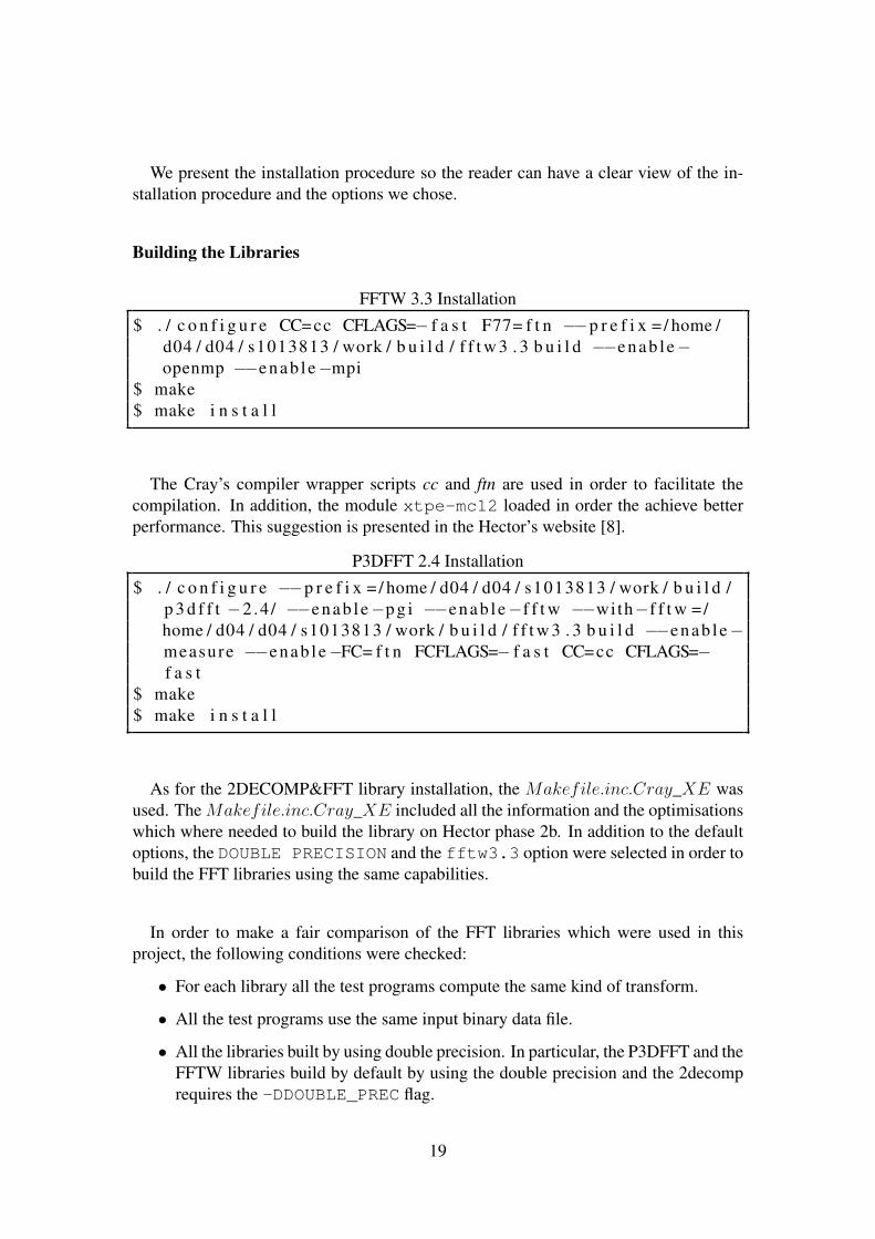
We present the installation procedure so the reader can have a clear view of the in-stallation procedure and the options we chose.

Building the Libraries

FFTW 3.3 Installation$ . / c o n f i g u r e CC=cc CFLAGS=− f a s t F77= f t n −−p r e f i x = / home /

d04 / d04 / s1013813 / work / b u i l d / f f t w 3 . 3 b u i l d −−enab l e−openmp −−enab l e−mpi

$ make$ make i n s t a l l

The Cray’s compiler wrapper scripts cc and ftn are used in order to facilitate thecompilation. In addition, the module xtpe-mc12 loaded in order the achieve betterperformance. This suggestion is presented in the Hector’s website [8].

P3DFFT 2.4 Installation$ . / c o n f i g u r e −−p r e f i x = / home / d04 / d04 / s1013813 / work / b u i l d /

p 3 d f f t −2 .4 / −−enab l e−p g i −−enab l e−f f t w −−with−f f t w =/home / d04 / d04 / s1013813 / work / b u i l d / f f t w 3 . 3 b u i l d −−enab l e−measure −−enab l e−FC= f t n FCFLAGS=− f a s t CC=cc CFLAGS=−f a s t

$ make$ make i n s t a l l

As for the 2DECOMP&FFT library installation, the Makefile.inc.Cray_XE wasused. The Makefile.inc.Cray_XE included all the information and the optimisationswhich where needed to build the library on Hector phase 2b. In addition to the defaultoptions, the DOUBLE PRECISION and the fftw3.3 option were selected in order tobuild the FFT libraries using the same capabilities.

In order to make a fair comparison of the FFT libraries which were used in thisproject, the following conditions were checked:

• For each library all the test programs compute the same kind of transform.

• All the test programs use the same input binary data file.

• All the libraries built by using double precision. In particular, the P3DFFT and theFFTW libraries build by default by using the double precision and the 2decomprequires the -DDOUBLE_PREC flag.

19

• Both P3DFFT and 2DECOMP FFT libraries linked to the FFTW 3.3 library.

• The argument FFTW_MEASURE used for planning on the FFTW. The P3DFFTrequires the --enable-measure and the 2DECOMP&FFT uses by defaultMEASURE for planning.

Finally, the test programs compiled by using hand-picked optimisation flags and com-pared to the libraries optimisation flags used in their examples.

3.2.4 Test Data

All the test programs required an input file which keeps the 3D input array. A separateprogram was implemented in order to generate a binary file containing the input data.

During the experiments, the same binary files (with dimensions 128× 128× 128 and256 × 256 × 256) were used as an input by all the test programs. In particular thisprogram uses the rand() function and initialises the buffer with real numbers from 0to 1.

Another program which read the data files (input or output) was implemented in orderto examine the data of these files at anytime. The main purpose of this program wasto observe the data during the debugging process and during the implementation of theproject.

Finally, the input and output data files were checked for errors by using the compareprogram. This program reads both input and output files and performs an one by onecomparison of each array’s data. The input and the output data stored separately in twobuffers, and each element of the input data buffer is compared to the output data buffer.The errors and the total number of errors are printed on the standard output.

3.2.5 Test Programs

Source Code Structure

A test program written in C programming language by using the Message Passing In-terface measured the performance of the FFTW 3.3 library. Two more similar programsimplemented for the P3DFFT and 2DECOMP&FFT libraries, but in this case the sourcecode of each program was written in Fortran 90 programming language. Both sourcecodes followed the ordinary structure of a common 3D FFT library test programs.

20

In this project the input data were not the data of a scientific problem but randomdata. This is not a disadvantage because most of the real world problems described bycomplex or real numbers. For this reason most of the benchmarking tests use randomdata as an input.

All the libraries provide functions for planning and executing the forward and thebackward plans. All these functions are built on the top of common MPI functions(except the OpenMP functions of the FFTW). On account of this, the computation partof these programs makes use each library’s functions.

As for the remaining tasks required by the programs, the MPI I/O and the other com-mon MPI functions were used in order to handle the I/O binary data files and someother tasks (for example the processors number, the time measure etc.). All these com-putations were not included in the time measure procedure.

Timing

The most important part of a benchmarking procedure is the correct measure of thetime required by each library for the computations. The FFT timing process we fol-lowed during this project reflects the performance of the FFT libraries as they use small3D FFTs of the same 3D array size i.e. 128×128×128 or 256×256×256 on differentnumber of nodes by using either one or more cores per node.

The FFT performance measured by the repeated computing of small 3D FFTs of sizesless equal to 256× 256× 256. The same input file created by the create.c program, wasused by all the test programs.

The time measuring part in each test program’s source code is measuring the exe-cution time for the forward and backward plans. The forward and the backward planscomputations is included inside a FOR LOOP and the number of iterations could besetted by the user. The time reported at the end of each test program is the average timeof all iterations.

As for the FFTW timing test, the planning time was excluded (both P3DFFT and2DECOMP plan once at the initialisation stage). The time in each program was mea-sured by using the MPI_Wtime() function. The same methodology used in the OpenMPFFTW test program where we used the OpenMP omp_get_wtime function.

21

The code structure followed for the time measuring of the computations in all the testprograms was:

Computation Time MeasureT=0DO FOR n ITERATIONS

T −= MPI_Wtime ( )CALL f o r w a r d _ t r a n s f o r m _ r 2 c (B , A)T += MPI_Wtime ( ). . .

T −= MPI_Wtime ( )CALL b a c k w a r d _ t r a n s f o r m _ c 2 r (A, B)T += MPI_Wtime ( )

END DO

Estimate versus Measure

The planning functions could make either use of the measure or the estimate argu-ment. As for the FFTW library, the FFTW_MEASURE argument requires the library toinvestigate the most efficient way to compute the fast Fourier transform for a specifichardware. This allows the test program to find the best way to compute the Fouriertransform of size N.

In contrast to the FFTW_MEASURE, the FFTW_ESTIMATE argument does not runany particular calculation, and uses directly a plan which is not as efficient as the optimalplan. Therefore, the FFTW_MEASURE argument was used in order to have an optimalplan for the computations of the transforms.

3.2.6 Scripts

Makefiles

A makefile for each library was used in order to built each test program. These make-files contained the path of each library, the compiler’s optimisation flags, the FFTWenvironmental flags and the compiler.

Jobs Submission

The data collection was the most time consuming procedure. Numerous tests hadto execute on Hector’s nodes. Each test program returns on the standard output the

22

processors grid, the decomposition and the average time of the iterations, which couldbe initialised from the user.

In addition, the task scheduler used in Hector, prints in the standard output manyother useful details such the total number of processors and the number of cores pernode. All these details were very useful during the classification of the obtained results.

A bash script was implemented for the FFTW OpenMP and MPI test programs. Thisscript automated the procedure of the tasks submissions. In addition, when the scriptfinishes and all the output files are in the folder, another bash script is parsing the filesand keeps the required data.

The other two libraries which supported the 2D decomposition, was required the testprogram to be compiled for every processors grid (except when the automated routinemode was selected in the 2DECOMP&FFT).

23

Chapter 4

Experimental Design

4.1 HPC Systems Architecture

The last two decades the HPC Systems are becoming a trend in the scientific world.Most of the universities and the research centres make use of machines which consist ofa large number of cluster nodes. The vast majority of those supercomputer’s nodes areSMP machines consist of one or more multicore processors. The architecture complex-ity of these systems, complicates the programming and makes difficult the utilization ofall the available computing resources.

Such machines can run parallel programs which require demanding computationsand numerous tasks. The supported programs usually, are using the Message PassingInterface or other models of parallelisation, in order to be executed in these parallelenvironments. In recent years there is great interest to search for the ideal programmingmodel of these supercomputers.

In the beginning of this section we present some specific information about theproject’s hardware and software and then we analyse how we setup the experimentand which arguments we use for different total cores and cubes combinations for eachdecomposition.

4.1.1 Hardware

The performance of the supercomputers is measured and listed in the TOP500.org [45].This test programs were executed on Hector Phase 2b which is one of the fastest super-computers of the TOP500 list, and the fastest supercomputing facility in the UnitedKingdom. The architecture features of Hector phase 2b summarised on table 4.1.

24

Cray XE6 system

Machine Number of Nodes 464 blades×4 nodesCores per Node 24 (2× 12core)

Processor

Processor Architecture AMD Opteron 64bitProcessor Model Magny CoursProcessor Cores 12Processors Frequency 2.1GHz

Memory Memory per Node 32Gb (2× 16Gb)Total Memory 59.4Tb

Table 4.1: Hector hardware specifications.

Distributed Memory Systems with SMP nodes

The structure of the modern supercomputer is very complex. In particular, each SMPsystem node includes everything from a two one-core processor or multiple processorsconsisting of multiple cores by using separate or the same main memory.

Machines like Cray XE6 consist of clusters of SMP nodes. In Hector each nodeconsists of two twelve-core processors. In particular, each one of the AMD’s Magny-Cours Opteron processors [46] has two dies each one is containing 6 cores. Inside theprocessor 12 MB of level 3 cache shared by both dies. Each one of these dies has 6MBlevel 3 cache and this capacity is shared by the six cores.

Each die in the processor has two memory channels and each one of these dies isa Non-Uniform Memory Access (NUMA) node. As a result each one of the nodesconsists of four NUMA regions.

Programming Clusters of Multicore-Nodes

The mixed environment of distributed SMP systems sometimes do not allow the pro-grams to scale above a large number of cores, therefore, the programming model whichbest suits on these hardware architectures is a very open-ended question.

Programming models such the Message Passing Interface are very common for theprograms in order to run on parallel machines like supercomputers. In particular MPIallowed the programs to scale up to thousands of processors and most of the programsin the scientific world are implemented by using MPI.

Recent work [47] and [48] have shown that the mixed mode programming model byusing the Message Passing Programming model for the inter-node programming and

25

a Shared Memory Programming model for the intra-node programming are offeringinteresting results.

4.1.2 Interconnection Network

As a CRAY XE6 machine Hector uses the Gemini Scalable interconnect [49]. TheGemini ASIC is designed to implement 107 of MPI messages per second. The mainadvantage of the Gemini Interconnect is that offers direct hardware support to the PGASlanguages (for example the UPC [50] and the Co-Array Fortran [51]). As expected,the programs which are written in one of these languages have better performance insystems with the Gemini Interconnect.

On a CRAY XE6 machine (for example Hector) each two nodes share a Gemini chipwhich has 10 links in order to implement a three dimensional torus of CPUs. On Hectorthe Gemini features summarised in the table 4.2.

MPI point-to-point bandwidth 5GB/s

Latency between 2 nodes 1− 1.5µs

Table 4.2: Gemini Interconnect on Hector phase 2b.

4.1.3 Compiler

The Portland Group compilers were used in order to compile the source codes. ThePGI compiler were available in Hector between many other compilers & tools. In addi-tion the Hector’s module environment used in order to manage the systems’s softwarecomponents.

The PGI compiler includes all the latest compiler optimisations which can be used bycalling the appropriate flag in the compilation. The main flags used in order to compilethe source codes were the -O3 and the -Mpreprocess. Those flags were also usedby the library’s examples.

Many other optimisation flags examined such the -fastsse, -Msmartalloc,-O2 and -Mipa=fast,inline without any performance improvement. Probably,that was the reason the 2DECOMP&FFT makefile for the Cray XE6 systems didn’tmake use these flags.

In addition many information about the compilation taken from the PGI, the Hector’sand the FFT libraries websites.

26

4.2 Experiments Setup

4.2.1 Testing Different Decompositions

In this report the 1D decomposition sometimes called a "slab decomposition". Inthis approach the first dimension of the input array is divided to the rows and each taskassigned a subset of the data. As discussed in section 2.4 the maximum number of thetasks is equal to the first dimension.

The 2D decomposition sometimes called a "rod decomposition" or "pencil decompo-sition" because the data are divided over the two dimensions and the maximum numberof processors depends on the 3D array dimensions.

The three programs which were used for the project (one for each library) requiredthe input binary data file, the parameters Prow, Pcol (processors grid), dimX, dimY, dimZ(dimensions of the 3D array) and the name of the output file.

For the 1D decomposition each test program executed by using up to 16 cores pernode on Hector for the test cases presented in table 4.3

Dimensions Prow × Pcol (Processors Grid) dimX, dimY, dimZ128× 128× 128 {1}× {1, 2, 4, 8, 16, 32, 64, 128} 128, 128, 128256× 256× 256 {1}× {1, 2, 4, 8, 16, 32, 64, 128, 256} 256, 256, 256

Table 4.3: 1D decomposition test parameters

For the 2D decomposition we implemented two phases of tests. The first phase wasan experimental phase. In particular, we changed the processors grid of each libraryby using all the possible combinations, in order to find how much the processors gridaffects the computational time required by the libraries. During this tests we used fixedarray dimensions and fixed number of cores (i.e. for 512 cores and 3D array withdimensions 256× 256× 256).

The results of these tests were analysed and used for the main testing procedure ofthe 2D decomposition, in order to used the optimal processors grid for each library andcollect the best possible timings.

In the second experiment where the 2D decomposition was used, each test programexecuted by using 1 and 16 cores per node on Hector for the test cases presented in thetable 4.4:

27

Dimensions Prow × Pcol (Processors Grid) dimX, dimY, dimZ128× 128× 128 Optimal Processors Grid 128, 128, 128256× 256× 256 Optimal Processors Grid 256, 256, 256

Table 4.4: 1D decomposition test parameters

During all the experiments, the number of iterations was fixed to 20. Moreover, eachtest program executed on the back-end nodes 20 times. The jobs submitted up to 16cores per Hector’s node (for the 1, 2, 4, 8, 16 total cores only one node used, except theexperiments with one core per node).

The timing results we presented in this report are the minimum average timings ofthe 20 iterations which achieved from the 20 times of each test program execution.

The majority of the experiments implemented by using up to 16 cores per node inHector. Each Hector’s node, as presented in table 4.1, consists of 24 cores. However,this number it is not convenient because it is not a power of 2. Therefore, it was diffi-cult to distribute equally the tasks to the nodes. In addition, this is one of the reasonsthe mixed mode programming models such the OpenMP/MPI developed, in order tooptimise the programs performance in such hardware architectures.

As a result, the maximum number of cores per node which belongs to the power of2 was the 16, and all the tests implemented by using 1, 2, 4, 8 and 16 cores per node.In addition, a number of experiments implemented in 24 cores per node in order toexamine the intra-node communications.

4.2.2 Reporting

All the test programs produce an output data file. This file was compared to the inputfile by using the program which implements the comparison, in order to find if there areany errors between the files. In addition, on the standard output we got the average timerequired for the computation.

Plots and Tables

Time – Cores and Speedup – Cores graphs were used in order to compare the perfor-mance of the FFT libraries. The graphs present the average time in order to be readable.In addition, tables present each experiment details and the speedup of the programswere used in order the reader to have all the information required for the understandingof the analysis.

28

The bold numbers in tables present the best time achieved across the libraries for thesame number of total cores, cores per node and cubes dimensions.

Speedup

The speedups presented in the tables in this report calculated by using the commonspeedup formula: Sp = T1

Tp, where the p is the total number of processors, T1 is the

execution time required by the sequential program and Tp is the execution time requiredby the parallel program using p number of processors.

Mflops

The megaflops performance during the FFT is calculated using the following for-mula:

MFlops ≈ 2.5 ∗Nlog2(N)

time10−3sec, N is the product of the FFT dimensions

MFlops is a scaled version of the speed and it is defined by the above formula, whichreferred to the real transform.

The radix-2 Cooley-Tukey FFT algorithm asymptotically requires 5Nlog2(N) float-ing point operations and the FFT MFlop estimate is used in most of the FFT benchmarkreports in order to compare the algorithm efficiency.

29

Chapter 5

Results and Performance Analysis

This chapter presents the results collected during the tests. Figures and tables wereused in order to describe the behaviour of each library. All the timings presented inthis chapter are referring to the performance of each library for the computation of theFourier transform of two 3D meshes with dimensions 256×256×256 and 128×128×128.

5.1 Slabs and Pencils on Hector

In the first two parts of this section we presented the results of the 1D decompositionalong with an analysis of the results. The other four parts are referring to the perfor-mance of the P3DFFT and 2DECOMP&FFT libraries by using the 2D decomposition(Rods or Pencils).

Finally, in the last section we present a comparison between the slab and the pencildecomposition after interpreting the obtained results from all the experiments in Hector.

5.1.1 1D Decomposition (Slab)

256× 256× 256 – 1 core per node

Table 5.1 shows the test programs timings by using only one core per node. Fromthe observed timings when one core per node was used, the libraries performance aspresented in the figure A.1 is almost identical. The timing needed from the FFTW onthe sequential code was the minimum between the libraries.

30

The experiments using from 2 to 128 nodes (cores) presented in 5.1, the P3DFFTlibrary performed better than the other two libraries. Furthermore, in the case of 256nodes (cores) the FFTW 3.3 library outperform the other two libraries. The FFTW 3.3,P3DFFT and 2DECOMP&FFT speedups were 95.68, 99.28 and 97.49 respectively.Figure 5.1 illustrates the speedups concerning these tests.

Cores FFTW SPEEDUP P3DFFT SPEEDUP 2DECOMP&FFT SPEEDUP1 1.1928 1.00 1.2954 1.00 1.3716 1.002 0.8936 1.33 0.7061 1.83 0.7220 1.904 0.4054 2.94 0.3658 3.54 0.3709 3.708 0.2157 5.53 0.1864 6.95 0.1897 7.2316 0.1132 10.54 0.0913 14.19 0.0979 14.0032 0.0535 22.28 0.0446 29.05 0.0470 29.1964 0.0292 40.81 0.0245 52.81 0.0263 52.20128 0.0185 64.39 0.0157 82.34 0.0167 82.23256 0.0125 95.68 0.0130 99.28 0.0141 97.49

Table 5.1: SLAB: 2563, 1 core per node, time and speedup.

1 2 4 8 16 32 64 128

256

0

20

40

60

80

100

Cores

Speedup

FFTWP3DFFT

2DECOMP&FFT

Figure 5.1: SLAB: Speedup using 2563 3D FFT with one core per node.

256× 256× 256 – 16 cores per node

Figure 5.2 presents the speedup of the libraries when up to 16 cores per node wereused. In particular, from 1 to 16 cores, one node was used for the experiments from 16to 256 cores, 16 cores per node were used (for example the 256 total cores distributed in

31

16 nodes). The FFTW library achieved the minimum sequential time and the P3DFFTachieved the minimum timings up to 256 total cores. In addition, the performance of the2DECOMP&FFT library was almost identical to the performance of the P3DFFT. TheFFTW, P3DFFT and 2DECOMP&FFT speedups as presented in table 5.2 were 34.95,55.50 and 56.02 respectively.

Cores FFTW SPEEDUP P3DFFT SPEEDUP 2DECOMP&FFT SPEEDUP1 1.1928 1.00 1.2954 1.00 1.3716 1.002 1.0435 1.14 0.7670 1.69 0.7330 1.874 0.5595 2.13 0.4615 2.81 0.4649 2.958 0.3809 3.13 0.2771 4.67 0.2798 4.9016 0.2089 5.71 0.1443 8.98 0.1481 9.2632 0.1296 9.20 0.0852 15.21 0.0875 15.6764 0.0847 14.09 0.0479 27.02 0.0489 28.03128 0.0440 27.08 0.0383 33.82 0.0422 32.53256 0.0341 34.95 0.0233 55.50 0.0245 56.02

Table 5.2: SLAB: 2563, 16 cores per node, time and speedup.

1 2 4 8 16 32 64 128

256

0

10

20

30

40

50

60

Cores

Speedup

FFTWP3DFFT

2DECOMP&FFT

Figure 5.2: SLAB: Speedup using 2563 3D FFT with 16 cores per node

128× 128× 128

This project focuses on small 3D FFTs. Therefore, it was necessary to experimentwith even smaller cubes. The same experiments were performed for the case of a 3Dmesh with dimensions 128 × 128 × 128. In the first experiment we used one core per

32

node and then 16 processors per node (from 1 to 16 cores total number of cores onlyone node was used).

128× 128× 128 – 1 core per node

Figure 5.3 shows the speedup during the experiment with 1283 cubes using one coreper node. When the test programs executed using only one core (sequential program),the FFTW completed the computations by using the minimum time compared to thesequential timings achieved by the other libraries.

From 2 to 64 cores, the performance of the P3DFFT and the 2DECOMP&FFT werealmost identical, with the P3DFFT achieving better timings during all the tests. Fig-ure A.3 and table 5.3 present the results in more detail.

Finally, when the maximum number of cores was used (128 because of the slab de-composition limit factor) the FFTW 3.3 test program outperform the other two libraries,and required less time to complete the Fourier transform computation.

Cores FFTW SPEEDUP P3DFFT SPEEDUP 2DECOMP&FFT SPEEDUP1 0.1324 1 0.1445 1 0.1554 12 0.0845 1.56 0.0792 1.8234 0.0806 1.924 0.0477 2.77 0.0387 3.7281 0.0397 3.908 0.0226 5.84 0.0178 8.0818 0.0194 7.9816 0.0117 11.31 0.0093 15.5040 0.0096 16.1432 0.0070 18.77 0.0050 28.8104 0.0051 29.9964 0.0048 27.32 0.0035 40.8118 0.0039 39.72128 0.0035 37.77 0.0040 36.0052 0.0044 35.23

Table 5.3: SLAB: 1283, one core per node, time and speedup.

128× 128× 128 – 16 cores per node

In the experiment where we computed the Fourier transform of a 3D mesh with di-mensions 128×128×128 by using 16 cores per node the FFTW achieved the minimumtiming by using 1 and 128 total cores. As we can see from the figure 5.4 in all the othertests the P3DFFT library requires the minimum time to complete the computations byusing different numbers of cores between 1 and 128, compared to the other two libraries.

Once again, the 2DECOMP&FFT according to the timings presented in the table 5.4had similar performance to the P3DFFT.

33

1 2 4 8 16 32 64 128

0

10

20

30

40

Cores

Speedup

FFTWP3DFFT

2DECOMP&FFT

Figure 5.3: SLAB: Speedup using 1283 3D FFT 1 core per node

Cores FFTW SPEEDUP P3DFFT SPEEDUP 2DECOMP&FFT SPEEDUP1 0.1325 1.00 0.1445 1.00 0.1555 1.002 0.0941 1.41 0.0851 1.70 0.0871 1.794 0.0657 2.02 0.0526 2.75 0.0554 2.808 0.0436 3.04 0.0317 4.56 0.0327 4.7516 0.0180 7.38 0.0151 9.60 0.0151 10.2932 0.0134 9.91 0.0093 15.48 0.0096 16.2664 0.0107 12.33 0.0066 21.91 0.0069 22.61128 0.0059 22.64 0.0087 16.54 0.0088 17.59

Table 5.4: SLAB: 1283, 16 cores per node, time and speedup.

Intra-Node Performance - 1D Decomposition

The test programs executed on Hector by using up to 16 cores per node for the com-putation of the FT of a 3D input array with dimensions 256 × 256 × 256, in order toanalyse the performance of the libraries using MPI. In addition to these tests, anothertest was implemented by using the openmp FFTW functions.

FFTW test program using the OpenMP was executed on up to 16 threads and theresults were compared to the MPI results from the other two libraries where up to 16MPI tasks was used. In addition, the results compared to the FFTW MPI results. Theobtained results were presented in table 5.5 and show that the FFTW OpenMP versionachieved the minimum timings for all the core/threads selection.

34

1 2 4 8 16 32 64 128

05· 10−2

0.1

0.15

Cores

Tim

e(sec)

FFTWP3DFFT

2DECOMP&FFT

Figure 5.4: Libraries performance using 1283 3D FFT 16 cores per node.

Finally, the figure A.4 shows that the OpenMP outperform all the other implemen-tations by using only one node, including those implementations are using the 2D de-composition.

Threads/Cores OpenMP MPIFFTW SPEEDUP FFTW P3DFFT 2DECOMP&FFT

1 1.1617 1 1.1928 1.2953 1.37152 0.6175 1.88 1.0434 0.7670 0.73294 0.3303 3.52 0.5595 0.4615 0.46498 0.1810 6.42 0.3808 0.2771 0.2798

16 0.1056 10.99 0.2089 0.1443 0.1480

Table 5.5: SLAB: 2563, FFTW OpenMP version versus MPI in one node.

5.1.2 1D Decomposition Performance Analysis

In general from the 1D decomposition results we can make a conclusion that:

SLAB: 256× 256× 256 – 1 core per node All the libraries had very good scaling.

SLAB: 256× 256× 256 – 16 cores per node P3DFFT and 2DECOMP&FFT test pro-grams had better speedup than the FFTW.

SLAB: 128× 128× 128 – 1 core per node FFTW test program scales better than theother two libraries test programs.

35

1 2 4 8 16 32 64 1280

5

10

15

20

Cores

Speedup

FFTWP3DFFT

2DECOMP&FFT

Figure 5.5: SLAB: Speedup using 1283 3D FFT 16 cores per node.

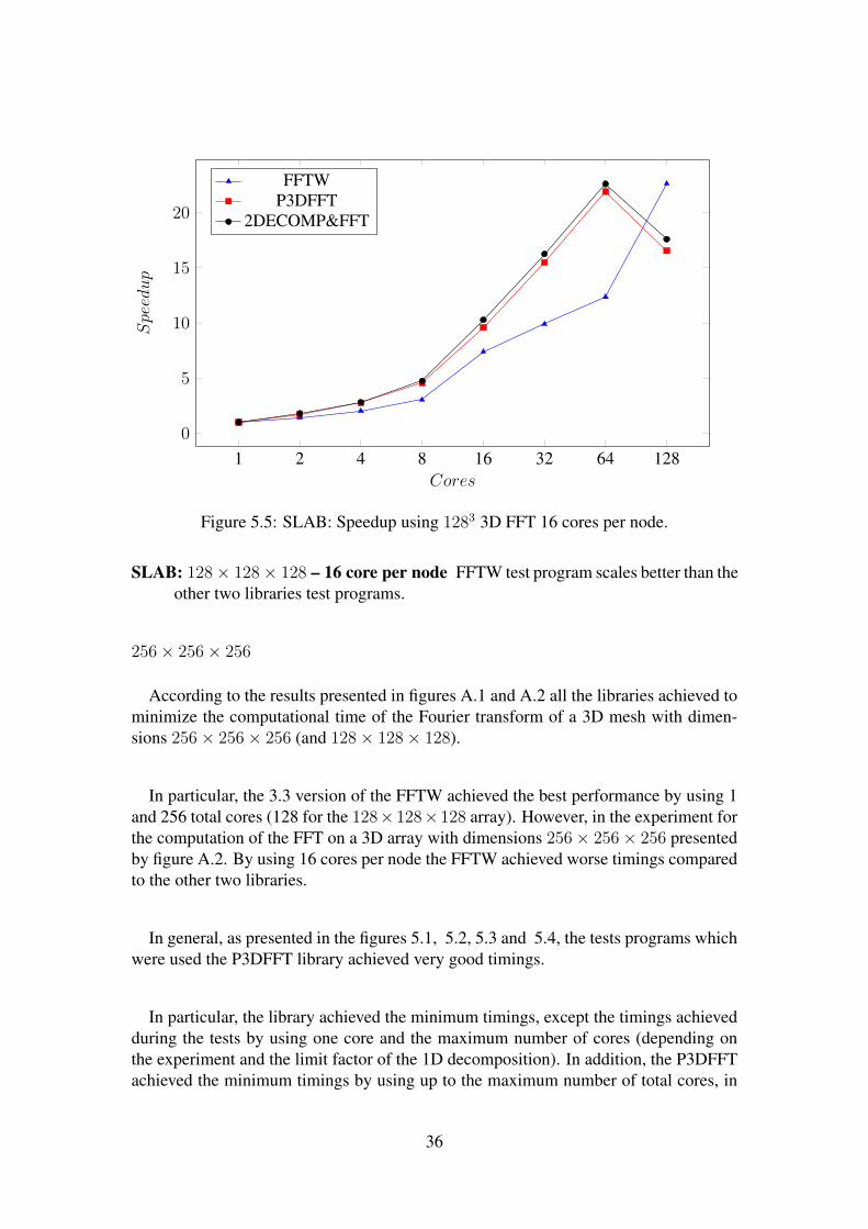
SLAB: 128× 128× 128 – 16 core per node FFTW test program scales better than theother two libraries test programs.

256× 256× 256

According to the results presented in figures A.1 and A.2 all the libraries achieved tominimize the computational time of the Fourier transform of a 3D mesh with dimen-sions 256× 256× 256 (and 128× 128× 128).

In particular, the 3.3 version of the FFTW achieved the best performance by using 1and 256 total cores (128 for the 128×128×128 array). However, in the experiment forthe computation of the FFT on a 3D array with dimensions 256× 256× 256 presentedby figure A.2. By using 16 cores per node the FFTW achieved worse timings comparedto the other two libraries.

In general, as presented in the figures 5.1, 5.2, 5.3 and 5.4, the tests programs whichwere used the P3DFFT library achieved very good timings.

In particular, the library achieved the minimum timings, except the timings achievedduring the tests by using one core and the maximum number of cores (depending onthe experiment and the limit factor of the 1D decomposition). In addition, the P3DFFTachieved the minimum timings by using up to the maximum number of total cores, in

36

order to complete the Fourier transform computation of a cube with dimensions 256×256× 256.

Furthermore, during the test using an input with dimensions 256 × 256 × 256, asthe number of cores increased the time required for the computations decreased. Thisbehaviour shows that the library scales well. The tables 5.1 and 5.2 present in detailthe speedups and the timings in each case.

The test programs implemented by using the 2DECOMP&FFT library recorded al-most identical timings to the P3DFFT. Moreover, in individual experiments the 2DE-COMP&FFT tests required less time to complete the computations.

128× 128× 128

It should also be noted that when the dimensions of the 3D input array reduced from256×256×256 to 128×128×128 the P3DFFT and the 2DECOMP&FFT, as presentedin the tables 5.3 and 5.4 both libraries achieved their minimum timings for 64 cores.Whereas, by using 128 total cores the performance decreased regardless the number ofcores per node.

On the contrary, during all the tests the FFTW test programs, minimise the computa-tional time as the total number of cores increased up to the maximum number of coresallowed by the 1D decomposition.

The analysis concerning the 3D array with dimensions 128 × 128 × 128 and thetables 5.3 and 5.4 show that the P3DFFT and 2DECOMP&FFT library test programswhich compute small 3D FFTs such 1283 did not scale well when the number of coresexceeds a number of cores depending on the 1D decomposition limit factor for thetotal tasks. In particular, there is a performance decrease after a number of total cores,regardless the number of cores per node were used.

Intra-Node 1D Decomposition Performance Analysis

The FFTW OpenMP version program achieved better timings compared to the MPItest versions of the other libraries including the FFTW’s test program written in MPI.The speedup of the FFTW’s test program written in OpenMP, as presented in the ta-ble 5.5, significant compared to the speedups and timings of the FFTW MPI version aspresented in table 5.2. The memory usage and the communications inside the node ofthe OpenMP function calls, are better than the MPI and let the algorithm to scale faster.

37

In particular, the FFTW MPI test program needs 16 cores to achieve the FFTWOpenMP test program’s performance using 8 threads (cores). A comparison betweenMPI and MPI/OpenMP for CRAY XE6 systems (reader can be referred to the [52]),concludes that the FFT computation programs using MPI/OpenMP scale better than thepure MPI implementations. In addition, the OpenMP model reduces the memory usageinside a node. To sum up, the MPI presented difficulty to scale further a number ofcores, especially for thousands of cores presented in the tables A.4 and A.1. In partic-ular, the performance depends on the 3D input array dimensions and the total numberof cores.

1D Decomposition - Conclusion

Summarizing the above analysis, the FFTW requires the minimum time to computethe Fourier transform of small cubes by using the maximum number of cores. Theother two libraries have very close behaviour and almost identical performance. Fromthe figures A.1, A.2, A.1 and A.2 it is difficult to distinguish one of them, but in themajority of the tests the P3DFFT achieved slightly better timings.

Another interesting point is that the timings achieved by the libraries by using onecore per node were better than the timings when up to 16 cores per node was used. Thisbehaviour is observed because of the memory access between the intra-node cores andthe demanding communications. In addition, the Gemini Interconnect minimises thecommunication overhead between the cluster nodes.

Finally, it is important to mention the timings achieved by the FFTW test programby using the FFTW’s OpenMP functions. These timings were the minimum timingsachieved during the 1D decomposition experiments 5.5 by using up to 16 cores pernode. The FFTW OpenMP functions are more efficient when applied on SMP hardwarearchitectures. This behaviour is due to the lack of replicated data and the intra-node MPIoverheads.

5.1.3 2D Decomposition (Rods or Pencils)

These sections present the performance of the P3DFFT and the 2DECOMP&FFTlibraries using 2D decomposition. The FFTW does not support 2D decomposition as aresult it was excluded from the experiment. However, for the benchmarking procedure,both libraries are built on the top of the FFTW 3.3.

This section is divided into two parts. In the beginning there is a description aboutthe processors grid selection and there is also a benchmark concerning the performanceof the libraries by using different processors grid (those applied on a fixed number of

38

cores by using a 3D array with dimensions 256× 256× 256. Furthermore, we analysedthe behaviour and the performance of each library.

In the second part we present the main benchmarking procedure were libraries usingthe 2D decomposition. The obtained results presented the performance of each one ofthe two libraries by using different numbers of total cores.

At the end of the section there is an extended analysis based on the overall librariesperformance using the pencil decomposition.

5.1.4 Processors Grid Selection

The processors grid selection has an important role in the computation of the Fouriertransform. As mentioned in the experimental analysis on section 4, many tests imple-mented in order to find the most efficient processors grid of each library by using a totalnumber of physical cores.

The 2DECOMP&FFT library supports an automated routine, where the library un-dertakes the task to find an ideal processors grid using a number of total cores.

The 2DECOMP&FFT automated routine seems to work very well for different sizesof 3D FFTs. Furthermore, the choice it is very efficient when thousands of cores wereused for the computations. In both libraries, the optimal 2D grid layout depends on thesystem’s software and hardware architecture and on each library’s architecture.

The correct choice of 2D processors grid can improve the communication efficiencyand the decomposition balance. As described in the P3DFFT library guide [53], for agiven grid of dimensions K × L × M , the decomposition sometimes it is not entirelyeven, as a result the elements are not divided equally to the tasks. In such cases, theload imbalance of the problem maximises and the program’s performance decreases. Inthis project the selected numbers were power of two, therefore, we didn’t have a suchproblem.

Figure 5.6 shows the possible options of the physical processors grid by using 1024cores (16 cores per node) for the computation of a 3D mesh with dimensions 256 ×256× 256.

39

From the timings indicated in figures 5.6 and A.9 (the same experiment with 512total cores) it is observed that for the particular occassion of the 2563 dimensions 3Dmesh for both libraries the ideal processors grid is about Prow � Pcol. Especially whenthe Prow × Pcol was 32x32 in figure 5.6 the timing achieved by each library was theminimum.

8x128 16x64 32x32 64x16 128x8

0.8

1

1.2

1.4

1.6

·10−2

ProcessorsGrid

Tim

e(sec)

P3DFFT2DECOMP&FFT

Figure 5.6: Libraries performance using 2563 3D array, 1024 total cores.

Processors Grid Analysis

As analysed in the 2decomp.org website [54] in order to achieve better performancea particular test in [54] shows that the Prow << Pcol is the better option to select theprocessors grid. In addition, in the "Processors Grid" page of the [54] noted that theProw value should be smaller than or equal to the number of the cores of each physicalprocessor. This remark concerning the CRAY XT4 machines with quad core processorswith SeaStar interconnection network.

In our project the test results presented in figures 5.6 and A.9 show that the Hector’sphase 2b interconnection network (Gemini) which used in CRAY XE6 supercomput-ers, optimise the inter-node communication performance (compared to the older inter-connects) and achieved better performance when the Prow is bigger than the physicalprocessors cores. The same remark observed in the report [55].

In addition, the non-uniform memory access (NUMA) arrangement seems to be lessefficient for the intra-node communications (because of the complexity of the AMD’s

40

Magni-Cours architecture [46]). However, when thousands of cores were used in orderto compute large 3D FFTs the Prow << Pcol it is preferred as reported from the timingson [54]. The computations seems to be more balanced by using this ratio.

The processors grid selection had similar affect on the performance of the P3DFFTlibrary. According to the presented results in [56] the performance increased when theProw << Pcol, and as presented in that project’s benchmarks, while the number ofthe processors increased the ideal processors grid converges to Prow � Pcol (for theparticular 3D FFTs used in this project). Figures 5.6 and A.9 present a similar responsebecause while the number of the cores increased from 512 to 1024 the best processorsgrid changed from Prow << Pcol (512 cores) to Prow � Pcol (1024 cores).

Finally, for each library the optimal processors grid depends mainly on the total num-ber of cores. For both libraries the Prow should be less or equal to the Pcol dependingon the total cores, the system hardware and the dimensions of the array. In the majorityof the occasions the optimal processor grid is when the Prow is less than or equal to thePcol.

5.1.5 2D Decomposition Performance

256× 256× 256 – 1 core per node

The timings for each experiment presented in table A.1 and figure 5.9 are concerningthe test programs which compute the Fourier transform of a 3D mesh with dimensions256×256×256. Especially, both libraries achieved their best timings by using 512 totalcores. In addition, the libraries achieved the timings presented in table A.2 by using thesame processors grid.

During the tests when using from 1 to 8 total cores, the P3DFFT had better perfor-mance compared to the 2DECOMP&FFT. When using from 16 to 512 cores the 2DE-COMP&FFT required less time to complete the computation. In addition, the 2DE-COMP&FFT requires less time to perform the computations compared to the P3DFFT.

256× 256× 256 – 16 cores per node

In the experiment where up to 16 cores per node were used, the 2DECOMP&FFTachieved the minimum timing by using 8192 total cores in order to execute the forwardand the backward plans (3D mesh with dimensions 256× 256× 256). In particular, asthe total number of cores increased up to 8192 total cores the performance of the testprogram was increased, as shown in the table A.1.

41

1 2 4 8 16 32 64 128 256 512 1024204840968192

050

100

150

200

250

300

Cores

Speedup

P3DFFT 1 core/nodeP3DFFT 16 cores/node

2DECOMP&FFT 1 core/node2DECOMP&FFT 16 cores/node

Figure 5.7: PENCIL: Speedup using 2563 3D FFT 1 and 16 cores per node.

The P3DFFT library had an almost identical performance to the 2DECOMP&FFT’sby using up to 4096 total cores. However, in this test case using 8192 cores the averagetime required by the library for the computations increased compared to the time re-quired when it used 4096 cores. During this experiment, the processors grid used fromboth libraries was the same.

128× 128× 128 – 1 core per Node

The performance of the libraries according to the figure 5.8 and the results presentedon table A.3 were similar. In particular, the P3DFFT test program achieved best resultswhen 1 and 512 cores were used. The computational time required by the test programdecreased as the number of the cores increased up to 512 cores in Hector.

The performance of the 2DECOMP&FFT library test program was similar to theP3DFFT’s performance. The test program scales well up to 256 cores when it achievedthe minimum required time for the computations. However, the performance decreaseswhen using 512 total cores. The result is presented in the table A.3.

The processors grid were used by each one of the test programs corresponding to theminimum average timings achieved by them are presented in table A.4.

42

128× 128× 128 – 16 cores per Node

Figure A.6 presents the performance of the test programs by using the P3DFFT andthe 2DECOMP&FFT in order to compute the Fourier computation of a 3D mesh withdimensions 128× 128× 128.

In this case, when 16 processors per node were used, the P3DFFT library had thebest performance when using 4096 cores and the 64 × 64 processors grid. After that,the performance decreased when using 8192 total cores.

In particular, using the P3DFFT library we observed that, as the number of processorsincreased the time required for the computations decreased. However, that happenedup to the 4096 cores. For the number of 8192 total cores the time required for thecomputations increased.

The 2DECOMP&FFT library achieved its minimum computational timing as pre-sented in table A.4 by using 2048 total cores (32× 64 processor grid). Finally, the pro-cessors grid used from both libraries confirms the results reported in the [56] and [54]regarding the optimal processors grid for each library.

1 2 4 8 16 32 64 128 256 512 1024204840968192

020

4060

80100

Cores

Tim

e(sec)

P3DFFT 1 core/nodeP3DFFT 16 cores/node

2DECOMP&FFT 1 core/node2DECOMP&FFT 16 cores/node

Figure 5.8: PENCIL: Speedup using 1283 3D FFT 1 and 16 cores per node.

43

5.1.6 2D Decomposition Performance Analysis

The obtained results presented in tables A.3, A.4, A.2 and A.1 show the performanceof the libraries for the computation of the Fourier transform of a 3D input array usingthe 2D decomposition (Pencil). Generally, the results shows that the test programsachieved to decrease the computational time of the Fourier transform as the number ofthe cores increased by using up to 16 cores per node.

256× 256× 256

The figure 5.7 shows that during the experiment with a 3D mesh larger than 128 ×128× 128 (256× 256× 256) the performance of the libraries had better scaling.

In contrast to the 128× 128× 128 test case, the 2DECOMP&FFT requires the min-imum time to complete the computations using 8192 cores (16 cores per node). Thistiming is the minimum recorded for the computation of the 3D array with dimensions256× 256× 256. As the number of cores increased (by using 1 and 16 cores per node),the time required by the library decreased .

2DECOMP&FFT for both tests achieved better timings by using 1 and 16 cores pernode, compared to the P3DFFT timings. However, the communication overhead of theFFT computation affected the performance and the time needed by the 512 cores (1core per node) is better compared to the time required by the library when 4096 coreswere used (16 cores per node).

The P3DFFT library when using 1 core per node had an almost identical performancewith 2DECOMP&FFT. However, when using 16 cores per node it appeared to have sim-ilar performance with 2DECOMP&FFT when up to 4096 cores were used (it requiredless time for the computations using 4096 cores compared to the 2DECOMP&FFT).Whereas, the communication overhead affected the performance and all the achievedtimings by using 8192 total cores (16cores per node) were close to 0.0082s which per-formance is similar to the time measured by using 512 total cores (16 cores per node).

128× 128× 128

The minimum timing achieved was the time required for the computations by theP3DFFT library by using 512 cores (1 core in node). The library required more timefor the computations when it uses 4096 cores (16 cores per node) compared to theexperiment with the 512 cores (1 core per node).

44

The 2DECOMP&FFT required more time for the computations using one core pernode, but it achieved a similar timing to the minimum P3DFFT timing, by using 256cores instead of the 512 cores required by the P3DFFT.

Tables A.4 and A.3 show that the performance of the 2DECOMP&FFT starts todecreases after the 2048 cores by using 16 cores per node (after the 256 cores by usingone core per node). The P3DFFT which had better performance in both tests seems tobe more efficient because its performance decreased after the 4096 cores when 16 coresper node were used, whereas up to the 512 total cores (1 core per node) there is not suchdecrease.

5.2 Slabs versus Pencils on Hector

In this section we summarised the analysis about the performance of the librariesby using either 1D or 2D decomposition. We wanted to make a comparison regardingwhich decomposition and which library required the minimum time for the Fouriertransform computation of the 3D mesh with dimensions 256 × 256 × 256 and 128 ×128× 128.

256× 256× 256

Regarding the Fourier transform computations of a 3D array with dimensions 256×256 × 256 the 2DECOMP&FFT achieved the minimum overall timing (0.0045s) byusing 8192 cores and the 2D decomposition. The same library achieved the secondminimum overall timing by using 512 core (1 core per node) and the 2D decomposition.

Slightly worse was the performance of the P3DFFT library. The library’s test pro-grams achieved their minimum timings by using 4096 total cores (16 cores per node)and 512 cores (1 core per node). Both timings achieved by using 2D decomposition andare presented in table 5.9.

In general, the 2D decomposition implementations achieved better timings comparedto the 1D decomposition. For the same number of nodes the FFTW timing was 0.0124s(best timing in 1D decomposition), whereas the P3DFFT timing was 0.0060s. TheFFTW by using 1D decomposition requires 51.62% more time to complete the compu-tation. In addition, the performance of the FFTW when using 256 nodes it is not themost cost efficient because it makes use of 1 core per node instead of 16 cores per node.

45

Table 5.6: 2563: 1D & 2D decomposition results.Library Time1 Cores2 Cores/Node Decomposition Nodes2DECOMP&FFT 0.0045 8192 16 2D 5122DECOMP&FFT 0.0057 512 1 2D 512P3DFFT 0.0060 4096 16 2D 256P3DFFT 0.0063 512 1 2D 512FFTW 0.0124 256+ 1 1D 256P3DFFT 0.0130 256 1 1D 2562DECOMP&FFT 0.0140 256 1 1D 256P3DFFT 0.0233 256 16 1D 162DECOMP&FFT 0.0244 256 16 1D 16FFTW 0.0341 256 16 1D 161 Libraries sorted by time.2 Total number of cores+ Maximum number of total cores (1D decomposition).

Figure 5.9 shows, another interesting point. The 2DECOMP&FFT is more efficienton the 2D decomposition when 16 cores per node were used. In contrast, the P3DFFTdoes not have very good scaling because after the 4096 total cores has a decrease inperformance.

Table 5.6 shows the minimum timings measured for each library during the tests, forboth 1D and 2D decomposition.

128× 128× 128

For small 3D FFTs with dimensions 128 × 128 × 128, the speedup of each libraryis illustrated in figure 5.10. In addition, table 5.7 presents the best timing achieved byeach library either using 1D or 2D decomposition.

The results obtained during this experiment are very valuable because they presentclearly each one of the behaviour of the libraries and how they are affected by thecommunication overhead.

The libraries achieved their minimum timings by using the 2D decomposition. Theminimum time achieved by using the 2D decomposition was the P3DFFT library using512 cores (1 core per node). The timing achieved by the FFTW 3.3 by using the 1Ddecomposition and 128 cores (1 core per node).

46

1 2 4 8 16 32 64 128 256 512 1024204840968192

050

100

150

200

250

300

Cores

Speedup

FFTW 1D 1 coreFFTW 1D 16 coresP3DFFT 1D 1 core

P3DFFT 1D 16 cores2DECOMP&FFT 1D 1 core

2DECOMP&FFT 1D 16 coresP3DFFT 2D 1 core

P3DFFT 2D 16 cores2DECOMP&FFT 2D 1 core

2DECOMP&FFT 2D 16 cores

Figure 5.9: Speedup using 2563 3D FFT 1-16 cores per node.

Another interesting result is that the 2DECOMP&FFT achieved a timing of 0.0015sby using 2D decomposition, while the FFTW achieved the timing 0.0035s by using 128cores (1 core per node). This result shows that the 2D decomposition achieved to over-come the 1D decomposition’s limit factor of 128 cores and reduce the computationaltime by 57.14% when using 256 cores (1 core per node).

In addition, the 2D decomposition outperforms the 1D decomposition by using afixed number of nodes. In particular, the minimum time achieved by the 1D decompo-sition was 0.0035s by using 128 cores (FFTW), whereas the 2D decomposition achieveda time around 0.0020s which is reduced is around 42.85%.

Further analysis involves the cost efficiency of the decompositions. The 0.0020srequired from the 2DECOMP&FFT library by using 2048 cores and 128 nodes (16cores per node) is not so important compared to the same library’s performance by usingonly 4 nodes and the 1D decomposition. The table 5.7 shows that the timing using 4nodes is similar for the P3DFFT’s. Such difference in timings is not so important inreal world simulations of this kind of 3D FFTs because the cost difference between 4and 128 nodes is disproportionate to the benefit of the decreased time.

Finally, comparing the performance of the decompositions as the cube’s dimensionsdecrease it is obvious that the communication overhead affects significantly the time

47

Table 5.7: 1283: 1D & 2D decomposition results.Library Time1 Cores2 Cores/Node Decomposition NodesP3DFFT 0.0013 512 1 2D 5122DECOMP&FFT 0.0015 256 1 2D 256P3DFFT 0.0017 4096 16 2D 2562DECOMP&FFT 0.0020 2048 16 2D 128FFTW 0.0035 128 1 1D 128P3DFFT 0.0035 64 1 1D 642DECOMP&FFT 0.0039 64 1 1D 64FFTW 0.0058 128+ 16 1D 8P3DFFT 0.0065 64 16 1D 42DECOMP&FFT 0.0068 64 16 1D 41 Libraries sorted by time.2 Total number of cores+ Maximum number of total cores (1D decomposition).

Nodes Total Cores Time Core/Node Library

512

8192 0.0024 16 P3DFFT512 0.0013 1 P3DFFT8192 0.0033 16 2DECOMP&FFT512 0.0019 1 2DECOMP&FFT

Table 5.8: 1283: 2D decomposition results for 512 Hector’s nodes.

required for the computations. However, as the dimensions increases the 2D decompo-sition takes advantage of the available cores and minimises the computations time.

Demanding Communications and Interconnection Network Performance

In order to investigate the affect of the Gemini Interconnect on the libraries perfor-mance we implemented another set of experiments. In the beginning of these experi-ments the total number of nodes was fixed to 512. The decomposition chosen for theexperiment was the 2D and the libraries were the P3DFFT and the 2DECOMP&FFT,because they support 2D decomposition. The 3D array dimensions were 128×128×128in order to understand the interconnect affect by using small 3D FFTs.

In table 5.2 the level which the Gemini Interconnect affected the results is clear.There is a decrease in the performance of the P3DFFT as the number of cores per nodeincreased up to 16. The performance decreased by 84.61%. The second library hada similar behaviour. As the cores per node increased up to 16 the performance of the2DECOMP&FFT decreased by 73.68%.

48

1 2 4 8 16 32 64 128 256 5121024

20484096

8192

020

4060

80100

Cores

Speedup

FFTW 1D 1 coreFFTW 1D 16 coresP3DFFT 1D 1 core

P3DFFT 1D 16 cores2DECOMP&FFT 1D 1 core

2DECOMP&FFT 1D 16 coresP3DFFT 2D 1 core

P3DFFT 2D 16 cores2DECOMP&FFT 2D 1 core

2DECOMP&FFT 2D 16 cores

Figure 5.10: Speedup using 1283 3D FFT, 1 and 16 cores per node.

By comparing the results which presented in figure 5.10, table 5.2 and table A.4,we observe that after a certain computation time between 0.0013s and 0.0017s bothlibraries could not achieve lower timings. Therefore, the interconnection network placesa limit in computation time because of the communication overhead. Thus, even thenumber of nodes or cores is increased the computation time can not reduced. Therefore,in the test case presented in table A.4 there is a performance decrease for both libraries.

Finally, the project [55] includes a performance comparison between the SeaStar andthe Gemini Interconnect and present the ability of the test program which make use theGemini Interconnect to scale almost ideal up to 10000 cores.

49

Chapter 6

Conclusions & Discussions

The results obtained during the project were very useful and let us make a numberof useful observations. The final thoughts about these observations are brought in thischapter which presents the conclusions we made after the results interpretation.

Finally, we discuss the goals of this project and we suggest some thoughts in order toimprove further the benchmarks.

6.1 Conclusions

The obtained results show that by using the slab decomposition, the FFTW 3.3achieved very good scaling both using small and medium size cubes (the 128×128×128and the 256× 256× 256). The other two libraries achieved similar performance to theFFTW and both had an almost identical performance.

As for the pencil decomposition, both P3DFFT and 2DECOMP&FFT had similarperformance. However, the communication overhead didn’t let the libraries to scalevery well after a certain number of cores depending on the cube size and the number ofcores per node.

Comparing the slab and the pencil decomposition, the pencil decomposition seemsto be more efficient and achieved to minimise the computation time because of the largetotal number of cores. However, as we reduced the size of the cubes the P3DFFT andthe 2DECOMP&FFT didn’t take advantage of the increased limit of tasks allowed bythe 2D decomposition, and they didn’t scale normally. In addition, from the resultsthe minimum timings by using either 1D or 2D were too close by using cubes withdimensions 128× 128× 128.

50

This means that probably for very small 3D FFTs (i.e. 323 or 643), the performanceof the libraries will be similar either using the 1D or the 2D decomposition.

During the investigation for the best processors grid for the 2D decomposition weconcluded that the 2DECOMP&FFT library’s routine which selects the processors gridworks very well, especially for large number of cores. The same processors grid af-fected in the same way the performance of the P3DFFT library.

The experiment with the FFTW’s OpenMP functions, showed that the shared mem-ory programming can outperform the MPI for the intra-node communications. Espe-cially, this makes very interesting the mixed-mode programming model performanceon the 3D FFTs computations.

The flexibility of the P3DFFT and 2DECOMP&FFT libraries by using either 1Dor 2D decomposition make them very efficient for the real world simulations whichusually, were described by large 3D FFTs.

In our project, when using the 2D decomposition, after a total number of cores thecommunication overhead didn’t allowed them to reduce further the computation time.On the other hand they outperform the 1D decomposition implementations. The dif-ference in time was increased as the dimensions increased. Therefore, for larger cubesdimensions (i.e. 2048 × 2048 × 2048 etc.) the computational time using the 2D de-composition compared to the 1D decomposition computation time will probably beperceivable to the end user.

To sum up, the Gemini Interconnect allowed the pencil decomposition to outperformthe slab decomposition for the certain 3D mesh dimensions we used. However, thenetwork set up a limit because the communication overhead didn’t allowed the librariesto scale after a number of cores. In addition, this limit was increased when the cube’sdimensions increased.

6.2 Discussions

Obviously, the interconnection network performance is an upper bound to the modernsupercomputerâAZs performance. The Gemini Interconnect achieved to set the upperbound higher according to the experimental results. By analysing the OpenMP testprogram speedup, we conclude that the network interconnect was not the only factorwhich affects the performance of the FFT computation. Therefore, the message pass-ing programming approach lacks of performance in the SMP systems compared to theOpenMP.

51

Unfortunately, in this project we didn’t succeed to implement the test programs byusing the hybrid OpenMP/MPI model. The main reason was that the FFTW 3.3 releasedon the 26th of July, and before the final version there wasn’t any documentation relatedto the new API.

In addition, the 3.3 Alpha version we used in the beginning of the project, was im-plemented by using the 3.2 MPI code. Therefore, the timings we had from the 3.3 alphahave changed when we used the 3.3 final version. As a result, we did the performancecomparison from the beginning because all the other libraries were built on the top ofthe 3.3 alpha.

Another problem which delayed the project was the fact that the obtained resultsdidn’t represent the performance of the libraries. This happened because on the FFTWtest program when we measured the time we included the time required for planning. Inaddition, we built the P3DFFT library without the --enable-measure flag whichenables the MEASURE, in order to have a better plan according to our hardware. How-ever, we found these problems and the final results represent the correct libraries per-formance for our experiments.

Finally, in the project plans was to implement the same benchmarking procedure inECDF Cluster "Eddie" [57]. However, problems during the installation and the diffi-culty to run jobs in the InfiniBand [58] didn’t allowed us to test our programs so manytimes and the obtained data were not reliable. In addition, the results obtained by usingthe Ethernet network in Eddie were not so interesting for our research. In particular, thenumber of cores using the InfiniBand (816 total cores - 68 nodes) was not comparableto the 8192 total cores we used for the 2D decomposition in Hector.

6.3 Future Work

In this project, the benchmarks was implemented using real data input, because theP3DFFT 2.4 does not support complex-to-complex transforms. Another benchmark canbe implement concerning complex number using the PFFT [59] instead of the P3DFFT.The PFFT library is developed from the Chemnitz University of Technology [60] andit is a higher-level library built on top of the FFTW 3.3. The main idea of these bench-marks is to use libraries which are built on the top of the new FFTW 3.3 library, in orderto examine the new APIs performance.

In addition, our project can be expanded by using the hybrid OpenMP/MPI program-ming model in order to compare the libraries and to compare the mixed mode results tothe MPI results. An interesting point is that the P3DFFT and the 2DECOMP&FFT does

52

not support an automated way to run tests using this programming model (the FFTW3.3 supports OpenMP). The results will be very interesting as presented in the [52].However, it will be a demanding project, and the final results and source codes can be acontribution to the libraries source codes.

Many supercomputer vendors have started to build clusters consist of powerful graphicprocessor units and many research centres such the National Supercomputing Center inTianjin [61] (China) runs the Tianhe-1A supercomputer [62] which consists of GPUs.These developments distracted of the High Performance Computing scientific worldand many researchers and industries have started to investigate the GPGPU program-ming approach further.

In particular, it will be very interesting as a further work to implement a benchmarkby using the most popular available GPGPU FFT libraries. Such an experiment will bevery interesting because the GPUs performance in raw numbers outperform the CPUsperformance. However, the programming models which should be used are in veryearly stages and especially the demanding communication of the FFTs will affect thescalability.

53

Appendix A

Results

A.1 1D and 2D decomposition results

1 2 4 8 16 32 64 128 256

0

0.2

0.4

0.6

0.8

1

1.2

1.4

Cores

Tim

e(sec)

FFTWP3DFFT

2DECOMP&FFT

Figure A.1: SLAB: Libraries performance using 2563 3D FFT with 1 core per node.

54

1 2 4 8 16 32 64 128 256

0

0.2

0.4

0.6

0.8

1

1.2

1.4

Cores

Tim

e(sec)

FFTWP3DFFT

2DECOMP&FFT

Figure A.2: SLAB: Libraries performance using 2563 3D FFT, 16 cores per node.

1 2 4 8 16 32 64 128

0

5 · 10−2

0.1

0.15

Cores

Tim

e(sec)

FFTWP3DFFT

2DECOMP&FFT

Figure A.3: SLAB: Libraries performance using 1283 3D FFT, one core per node.

55

1 2 4 8 16

00.2

0.4

0.6

0.8

11.2

1.4

Cores

Speedup

FFTW OpenMP 1DFFTW MPI 1D

P3DFFT MPI 1D2DECOMP&FFT MPI 1D

P3DFFT MPI 2D2DECOMP&FFT MPI 2D

Figure A.4: OpenMP performance versus the MPI implementations up to 16 cores -2563 3D FFT.

Cores P3DFFT SPEEDUP 2DECOMP&FFT SPEEDUP1 1.2954 1.00 1.3716 1.002 0.7670 1.69 0.7330 1.874 0.6191 2.09 0.6238 2.208 0.4006 3.23 0.4049 3.3916 0.2171 5.97 0.2197 6.2432 0.1177 11.01 0.1190 11.5364 0.0683 18.97 0.0697 19.69128 0.0396 32.72 0.0366 37.48256 0.0196 66.05 0.0196 70.08512 0.0096 134.34 0.0106 129.381024 0.0081 159.36 0.0079 173.662048 0.0074 174.68 0.0070 197.244096 0.0060 215.17 0.0065 210.138192 0.0082 141.32 0.0046 299.30

Table A.1: PENCIL: 2563, 16 cores per node, time and speedup.

56

Cores P3DFFT SPEEDUP 2DECOMP&FFT SPEEDUP1 1.2954 1.00 1.3716 1.002 0.7061 1.83 0.7220 1.904 0.4453 2.91 0.4466 3.078 0.2291 5.66 0.2262 6.0616 0.1202 10.78 0.1182 11.6132 0.0595 21.79 0.0602 22.7764 0.0298 43.52 0.0310 44.17128 0.0161 80.63 0.0163 84.37256 0.0090 144.62 0.0086 159.78512 0.0063 205.21 0.0058 238.46

Table A.2: PENCIL: 2563, one core per node, time and speedup.

Cores P3DFFT SPEEDUP 2DECOMP&FFT SPEEDUP1 0.1445 1.00 0.1555 1.002 0.0793 1.82 0.0807 1.934 0.0502 2.88 0.0511 3.048 0.0249 5.80 0.0247 6.2916 0.0124 11.64 0.0125 12.4132 0.0066 22.01 0.0073 21.2264 0.0034 42.56 0.0034 46.38128 0.0026 55.41 0.0024 65.24256 0.0023 64.00 0.0015 102.69512 0.0013 108.89 0.0019 80.78

Table A.3: PENCIL: 1283, one core per node, time and speedup.

57

P3DFFT 2DECOMP&FFTCores Processors Grid Time Speedup Processors Grid Time Speedup1 1x1 0.1445 1.00 1x1 0.1555 1.002 1x2 0.0851 1.70 1x2 0.0871 1.794 2x2 0.0785 1.84 2x2 0.0765 2.038 2x4 0.0528 2.74 2x4 0.0506 3.0716 4x4 0.0247 5.86 4x4 0.0237 6.5732 4x8 0.0124 11.68 2x16 0.0136 11.4164 8x8 0.0067 21.70 8x8 0.0074 21.00128 4x32 0.0042 34.30 4x32 0.0040 38.41256 8x32 0.0039 37.44 8x32 0.0030 52.41512 8x64 0.0026 54.62 8x64 0.0027 56.761024 16x64 0.0026 56.02 16x64 0.0025 61.982048 32x64 0.0022 64.64 32x64 0.0020 76.684096 64x64 0.0017 84.33 64x64 0.0031 50.208192 64x128 0.0024 60.63 64x128 0.0033 47.01

Table A.4: PENCIL: 1283, 16 cores per node, time and speedup.

1 2 4 8 16 32 64 128 256 512

05· 10−2

0.1

0.15

Cores

Tim

e(sec)

P3DFFT 1 core/node2DECOMP&FFT 1 core/node

Figure A.5: PENCIL: Libraries performance using 1283 3D FFT, one core per node.

58

1 2 4 8 16 32 64 128 256 512 1024204840968192

05· 10−2

0.1

0.15

Cores

Tim

e(sec)

P3DFFT 16 cores/node2DECOMP&FFT 16 cores/node

Figure A.6: PENCIL: Libraries performance using 1283 3D FFT, 16 cores per node.

1 2 4 8 16 32 64 128 256 512

00.2

0.4

0.6

0.8

11.2

1.4

Cores

Tim

e(sec)

P3DFFT 1 core/node2DECOMP&FFT 1 core/node

Figure A.7: PENCIL: Libraries performance using 2563 3D FFT, one core per node.

59

1 2 4 8 16 32 64 128 256 512 1024204840968192

0

0.2

0.4

0.6

0.8

1

1.2

1.4

Cores

Tim

e(sec)

P3DFFT 16 cores/node2DECOMP&FFT 16 cores/node

Figure A.8: PENCIL: Libraries performance using 2563 3D FFT, 16 cores per node.

4x128 8x64 16x32 32x16 64x8 128x41

1.2

1.4

1.6

1.8

2

2.2·10−2

Cores

Tim

e(sec)

P3DFFT2DECOMP&FFT

Figure A.9: Libraries performance using 2563 3D FFT, 512 total cores.

60

Bibliography

[1] “IEEE Standard for Information Technology - Portable Operating System Inter-face (POSIX(R)) System Administration - Part 3: User and Group Account Ad-ministration,” IEEE Std 1387.3-1996, p. 0_1, 1997.

[2] MPI Forum, “MPI: A Message passing interface,” in Supercomputing ’93 Confer-ence, 1993.

[3] L. Dagum and R. Menon, “OpenMP: an industry standard API for shared-memoryprogramming,” Computational Science Engineering, IEEE, vol. 5, no. 1, pp. 46 –55, jan-mar 1998.

[4] NVIDIA, “The CUDA homepage,” 2007. [Online]. Available: http://www.nvidia.com/object/cuda_home.html

[5] M. Frigo and S. G. Johnson, “FFTW for version 3.3,” 2011. [Online]. Available:http://www.fftw.org/

[6] D. Pekurovsky, “Parallel Three-Dimensional Fast Fourier Transforms (P3DFFTfor version 2.4).” [Online]. Available: http://code.google.com/p/p3dfft/

[7] N. Li and S. Laizet, “2DECOMP&FFT - A highly scalable 2D decomposition li-brary and FFT interface,” in Cray User Group 2010 conference, Edinburgh, 2010.[Online]. Available: http://www.2decomp.org/pdf/17B-CUG2010-paper-Ning_Li.pdf

[8] “HECTOR: UK National Supercomputing Service.” [Online]. Available:http://www.hector.ac.uk/

[9] J. Cooley and J. Tukey, “An Algorithm for the Machine Calculation of ComplexFourier Series,” Mathematics of Computation, vol. 19, no. 90, pp. 297–301, 1965.

[10] C. L. G.C. Danielson, “Some Improvements in Practical Fourier Analysis andTheir Application to X-ray Scattering From Liquids,” vol. 233, no. 4 and 5, pp.365–380 and 435–452, April and May 1942.

[11] M. Eleftheriou, J. Moreira, B. Fitch, and R. Germain, “A Volumetric FFTfor BlueGene/L,” in High Performance Computing - HiPC 2003, ser. LectureNotes in Computer Science, T. Pinkston and V. Prasanna, Eds. Springer Berlin/ Heidelberg, 2003, vol. 2913, pp. 194–203, 10.1007/978-3-540-24596-4_21.[Online]. Available: http://dx.doi.org/10.1007/978-3-540-24596-4_21

61

[12] M. Eleftheriou, B. G. Fitch, A. Rayshubskiy, T. J. C. Ward, and R. S.Germain,“Performance Measurements of the 3D FFT on the Blue Gene/L Supercomputer,”in Euro-Par’05, 2005, pp. 795–803.

[13] H. Jagode, “Fourier Transforms for the BlueGene/L Communications Network,”Master’s thesis, University of Edinburgh, 2006. [Online]. Available: http://www2.epcc.ed.ac.uk/msc/dissertations/dissertations-0506/hjagode.pdf

[14] B. W. Kernighan and D. Ritchie, “The c programming language,” 1978.

[15] W. H. Press and N. R. S. Firm. (1996) Numerical recipes in FORTRAN 77 andFORTRAN 90 the art of scientific and parallel computing.

[16] “Engineering and Scientific Subroutine Library (ESSL) and Parallel ESSL.”[Online]. Available: http://www-03.ibm.com/systems/software/essl/

[17] “AMD Core Math Library (ACML).” [Online]. Available: http://developer.amd.com/libraries/acml/pages/default.aspx

[18] “Intel Integrated Performance Primitives (Intel IPP) 7.0.” [Online]. Available:http://software.intel.com/en-us/articles/intel-ipp/

[19] “Intel Math Kernel Library (Intel MKL).” [Online]. Available: http://software.intel.com/en-us/articles/intel-mkl/

[20] Nvidia, “CUDA CUFFT Library,” 2007.

[21] “Nvidia official webpage.” [Online]. Available: http://www.nvidia.com

[22] “GPUFFTW: High Performance Power-of-Two FFT Library using GraphicsProcessors.” [Online]. Available: http://gamma.cs.unc.edu/GPUFFTW/

[23] A. Nukada and S. Matsuoka, “NukadaFFT: An Auto-Tuning FFT Library forCuda GPUs,” in GPU Technology Conference 2010, 2010.

[24] “DiGPUFFT – Distributed GPU 3D FFT.” [Online]. Available: http://code.google.com/p/digpufft/

[25] “Massachusetts Institute of Technology, (MIT).” [Online]. Available: http://web.mit.edu/

[26] “Cilk.” [Online]. Available: http://supertech.csail.mit.edu/cilk/index.html

[27] “FFTW: Speed Results.” [Online]. Available: http://www.fftw.org/speed/

[28] M. Frigo and S. Johnson, “The Design and Implementation of FFTW3,” Proceed-ings of the IEEE, vol. 93, no. 2, pp. 216 –231, feb. 2005.

[29] X. Leroy, “The Caml Light system release 0.71,” Mar. 1996.

[30] M. Frigo, “A fast Fourier transform compiler,” in Proceedings of theACM SIGPLAN 1999 conference on Programming language design andimplementation, ser. PLDI ’99. New York, NY, USA: ACM, 1999, pp. 169–180.[Online]. Available: http://doi.acm.org/10.1145/301618.301661

62

[31] H. Sorensen, D. Jones, M. Heideman, and C. Burrus, “Real-valued fast Fouriertransform algorithms,” Acoustics, Speech and Signal Processing, IEEE Transac-tions on, vol. 35, no. 6, pp. 849 – 863, jun 1987.

[32] C. Temperton, “Fast mixed-radix real fourier transforms,” Journal of Compu-tational Physics, vol. 52, no. 2, pp. 340 – 350, 1983. [Online]. Available:http://www.sciencedirect.com/science/article/pii/0021999183900347

[33] G. D. Bergland, “Numerical Analysis: A fast fourier transform algorithmfor real-valued series,” Commun. ACM, vol. 11, pp. 703–710, October 1968.[Online]. Available: http://doi.acm.org/10.1145/364096.364118

[34] P. N. Swarztrauber, Vectorizing the FFTs. Academic Press, New York, 1982, pp.51 – 83.

[35] C. Rader, “Discrete Fourier transforms when the number of data samples isprime,” Proceedings of the IEEE, vol. 56, no. 6, pp. 1107 – 1108, june 1968.

[36] “University of California, San Diego homepage.” [Online]. Available: http://www.ucsd.edu/

[37] “Google’s official developer site.” [Online]. Available: http://code.google.com/

[38] K. Kandalla, H. Subramoni, K. Tomko, D. Pekurovsky, N. Dandapanthula, S. Sur,and D. K. Panda, “Improving Parallel 3D FFT Performance using Hardware Of-floaded Collective Communication on Modern InfiniBand Clusters,” Ohio StateUniversity, Tech. Rep., Nov. 2010.

[39] D. A. Donzis, P. K. Yeung, and D. Pekurovsky, “Turbulence Simulations onO(104) Processors,” Jun. 2008.

[40] “NAG Fortran Compiler.” [Online]. Available: http://www.nag.co.uk/nagware/np.asp

[41] “benchFFT.” [Online]. Available: http://www.fftw.org/benchfft/

[42] “PGI Optimizing Fortran, C and C++ Compilers & Tools.” [Online]. Available:http://www.pgroup.com/

[43] “CRAY: The Supercomputer Company,” CRAY. [Online]. Available: http://www.cray.com/

[44] “Cray XE6 system,” CRAY. [Online]. Available: http://www.cray.com/Products/XE/CrayXE6System.aspx

[45] “Top 500 Supercomputer Sites.” [Online]. Available: http://www.top500.org/

[46] T. Carver, “Magny-Cours and Direct Connect Architecture 2.0.” [Online].Available: http://developer.amd.com/zones/magny-cours/pages/default.aspx

[47] L. Smith and M. Bull, “Development of mixed mode mpi / openmp applications,”in In WOMPAT 2000, 2000, pp. 6–7.

63

[48] J. D. Lorna Smith, Mark Bull, “Mixed mode programming on a clustered p690system,” in 9th IBM System Scientific Computing User Group (SCICOMP9),Bologne, Italy, 2004.

[49] R. D. Chamberlain, M. A. Franklin, and C. S. Baw, “Gemini: an optical intercon-nection network for parallel processing,” Parallel and Distributed Systems IEEETransactions on, vol. 13, no. 10, pp. 1038–1055, 2002.

[50] T. El-Ghazawi and L. Smith, “Upc: unified parallel c,” in Proceedings of the 2006ACM/IEEE conference on Supercomputing, ser. SC ’06. New York, NY, USA:ACM, 2006. [Online]. Available: http://doi.acm.org/10.1145/1188455.1188483

[51] C. Coarfa, Y. Dotsenko, J. Eckhardt, and J. Mellor-crummey, “Co-array fortranperformance and potential: An npb experimental study,” in In Proc. of the 16thIntl. Workshop on Languages and Compilers for Parallel Computing, number2958 in LNCS. Springer-Verlag, 2003, pp. 2–4.

[52] I. Bethune, “Improving the Performance of CP2K on the Cray XT,” in Cray UserGroup meeting (CUG), Edinburgh, UK, 2010.

[53] D. Pekurovsky, “P3DFFT user guide 2.4.” [Online]. Available: http://p3dfft.googlecode.com/files/P3DFFT_USER_GUIDE_2.4.pdf

[54] “2DECOMP&FFT website: Library for 2d pencil decomposition and distributedFast Fourier Transform.” [Online]. Available: http://www.2decomp.org/

[55] N. Li, “Direct Numerical Simulations (DNS) of Turbulent Fluid Flows - a sCSEProject,” February 2011.

[56] D. Pekurovsky, “Ultrascalable Fourier Transforms in Three Dimensions,” in Ter-aGrid ’11: Extreme Digital Discovery, Salt Lake City, Utah, 07/20/2011 2011.

[57] “Edinburgh Compute and Data Facility (ECDF).” [Online]. Available: https://www.wiki.ed.ac.uk/display/ecdfwiki/Home

[58] “InfiniBand.” [Online]. Available: http://www-03.ibm.com/systems/bladecenter/hardware/openfabric/infiniband.html

[59] “PFFT : parallel three-dimensional FFT software library.” [Online]. Available:http://www-user.tu-chemnitz.de/~mpip/software.php

[60] [Online]. Available: http://www-user.tu-chemnitz.de/

[61] “National Supercomputing Center,” Tianjin, China. [Online]. Available:http://www.nscc-tj.gov.cn/

[62] “Tianhe-1a,” National Supercomputing Center in Tianjin, Tianjin, China.[Online]. Available: http://www.nscc-tj.gov.cn/en/

64