parallel gibbs sampling: from colored fields to thin junction

324

Parallel Gibbs Sampling: From Colored Fields to Thin Junction Trees

Joseph E. Gonzalez Yucheng Low Arthur Gretton1 Carlos GuestrinCarnegie Mellon University

[email protected] Mellon University

[email protected] Unit, UCL

[email protected] Mellon University

[email protected]

Abstract

We explore the task of constructing a paral-lel Gibbs sampler, to both improve mixing andthe exploration of high likelihood states. Recentwork in parallel Gibbs sampling has focused onupdate schedules which do not guarantee con-vergence to the intended stationary distribution.In this work, we propose two methods to con-struct parallel Gibbs samplers guaranteed to drawfrom the targeted distribution. The first method,called the Chromatic sampler, uses graph col-oring to construct a direct parallelization of theclassic sequential scan Gibbs sampler. In thecase of 2-colorable models we relate the Chro-matic sampler to the Synchronous Gibbs sam-pler (which draws all variables simultaneouslyin parallel), and reveal new ergodic properties ofSynchronous Gibbs chains. Our second method,the Splash sampler, is a complementary strategywhich can be used when the variables are tightlycoupled. This constructs and samples multipleblocks in parallel, using a novel locking proto-col and an iterative junction tree generation al-gorithm. We further improve the Splash samplerthrough adaptive tree construction. We demon-strate the benefits of our two sampling algorithmson large synthetic and real-world models using a32 processor multi-core system.

1 INTRODUCTIONGibbs sampling is a popular MCMC inference procedureused widely in statistics and machine learning. On manymodels, however, the Gibbs sampler can be slow mixing[Kuss and Rasmussen, 2005, Barbu and Zhu, 2005]. Con-sequently, a number of authors [Doshi-Velez et al., 2009,Newman et al., 2007, Asuncion et al., 2008, Yan et al.,

Appearing in Proceedings of the 14th International Conference onArtificial Intelligence and Statistics (AISTATS) 2011, Fort Laud-erdale, FL, USA. Volume 15 of JMLR: W&CP 15. Copyright 2011by the authors.

2009] have proposed parallel methods to accelerate Gibbssampling. Unfortunately, most of the recent methods relyon Synchronous Gibbs updates that are not ergodic, andtherefore generate chains that do not converge to the tar-geted stationary distribution.

In this work we propose two separate ergodic parallelGibbs samplers. The first, called the Chromatic sampler,applies a classic technique relating graph coloring to paral-lel job scheduling, to obtain a direct parallelization of theclassic sequential scan Gibbs sampler. We show that theChromatic sampler is provably ergodic and provide strongguarantees on the parallel reduction in mixing time.

For the relatively common case of models with two-colorable Markov random fields, the Chromatic samplerprovides substantial insight into the behavior of the non-ergodic Synchronous Gibbs sampler. We show that in thetwo-colorable case, the Synchronous Gibbs sampler isequivalent to the simultaneous execution of two indepen-dent Chromatic samplers and provide a method to recoverthe corresponding ergodic chains. As a consequence, weare able to derive the invariant distribution of the Syn-chronous Gibbs sampler and show that is ergodic with re-spect to functions over single variable marginals.

The Chromatic sampler achieves a linear increase in therate at which samples are generated and is therefore idealfor models where the variables are weakly coupled. How-ever, for models with strongly coupled variables, the chaincan still mix prohibitively slowly. In this case, it is oftennecessary to jointly sample large subsets of related randomvariables [Barbu and Zhu, 2005, Jensen and Kong, 1996] inwhat is known as a blocking Gibbs sampler.

Our second parallel Gibbs sampler, the Splash sampler,addresses the challenges of highly correlated variables byincrementally constructing multiple bounded tree-widthblocks, called Splashes, and then jointly sampling eachSplash using parallel junction-tree inference and backward-sampling. To ensure that multiple simultaneous Splashesare conditionally independent (and hence that the chain isergodic), we introduce a Markov blanket locking proto-col. To accelerate burn-in and ensure high likelihood states

1Affiliated with CMU and MPI for Biological Cybernetics

325


are reached quickly, we introduce a vanishing adaptationheuristic for the initial samples of the chain, which explic-itly builds blocks of strongly coupled variables.

We provide a highly tuned open-source implementation ofboth parallel samplers using the new GraphLab framework[Low et al., 2010] for parallel machine learning, and com-pare performance on synthetic and real-world samplingproblems using a 32 processor multicore system. We findthat both algorithms achieve strong speedups in samplegeneration, and the adaptive Splash sampler can further ac-celerate mixing on strongly correlated models. Our exper-iments illustrate that the two sampling strategies comple-ment each other: for weakly coupled variables, the Chro-matic sampler performs best, whereas the Splash sampleris needed when strong dependencies are present.

2 THE GIBBS SAMPLERIn this work we focus on large probabilistic models that canbe represented as factorized distributions of the form:

π (x1, . . . , xn) ∝∏

A∈F

fA(xA), (2.1)

where each clique A ∈ F is a subset, A ⊆ 1, . . . , n,of indices and the factors fA are un-normalized positivefunctions, fA : xA → R+ over subsets of random vari-ables. While we will only consider discrete random vari-ables Xi ∈ Ω, most of the techniques can be directly ap-plied to continuous random variables.

Because the independence structure of Eq. (2.1) is cen-tral to the design of efficient parallel Gibbs samplers, wewill rely heavily on the Markov Random Field (MRF).The MRF of π is an undirected graph over the variableswhere Xi is connected to Xj if there is a A ∈ F such thati, j ∈ A. The set of all variables XNi adjacent to variableXi is called the Markov Blanket of Xi. A variable Xi isconditionally independent of all other variables given itsMarkov Blanket:

π (Xi |XNi) = π (Xi |X−i) (2.2)

where X−i refers to the set of all variables excluding thevariable Xi.

The Gibbs sampler, introduced by Geman and Geman[1984], is a popular Markov Chain Monte Carlo (MCMC)algorithm used to simulate samples from the joint distri-bution π. The Gibbs sampler is constructed by iterativelysampling each variable,

Xi ∼ π (Xi |XNi = xNi) ∝∏

A:i∈A,A∈F

fA(Xi,xNi)

(2.3)given the assignment to the variables in its Markov blanket.Geman and Geman [1984] showed that if each variable issampled infinitely often and under reasonable assumptions

Algorithm 1: The Synchronous Gibbs Samplerforall Variables Xj do in parallel1

Execute Gibbs Update: X(t+1)j ∼ π

(Xj |x(t)

Nj

)2

barrier end3

on the conditional distributions (e.g., positive support), theGibbs sampler is ergodic (i.e., it converges to the true distri-bution). While we have considerable latitude in the updateschedule, we shall see in subsequent sections that certainupdates must be treated with care: in particular, Geman andGeman were incorrect in their claim that parallel simulta-neous sampling of all variables (the Synchronous update)yields an ergodic chain.

For large models with complex dependencies, the mixingtime and even the time required to obtain a high likeli-hood sample can be substantial. Therefore, we would liketo use parallel resources to increase the speed of the Gibbssampler. The simplest method to construct a parallel sam-pler is to run a separate chain on each processor. However,running multiple parallel chains requires large amounts ofmemory and, more importantly, is not guaranteed to accel-erate mixing or the production of high-likelihood samples.As a consequence, we focus on single chain parallel ac-celeration, where we apply parallel methods to increase thespeed at which a single Markov chain is advanced. The sin-gle chain setting ensures that any parallel speedup directlycontributes to an equivalent reduction in the mixing time,and the time to obtain a high-likelihood sample.

Unfortunately, recent efforts to build parallel single-chainGibbs samplers have struggled to retain ergodicity. The re-sulting methods have relied on approximate sampling algo-rithms [Asuncion et al., 2008] or proposed generally costlyextensions to recover ergodicity [Doshi-Velez et al., 2009,Newman et al., 2007, Ferrari et al., 1993]. A central ob-jective in this paper is to design an efficient parallel Gibbssamplers while ensuring ergodicity.

3 THE CHROMATIC SAMPLERA naive single chain parallel Gibbs sampler is obtained bysampling all variables simultaneously on separate proces-sors. Called the Synchronous Gibbs sampler, this highlyparallel algorithm (Alg. 1) was originally proposed by Ge-man and Geman [1984]. Unfortunately the extreme paral-lelism of the Synchronous Gibbs sampler comes at a cost.As others [e.g., Newman et al., 2007] have observed, onecan easily construct cases (see Appendix A) where the Syn-chronous Gibbs sampler is not ergodic and therefore doesnot converge to the correct stationary distribution.

Fortunately, the parallel computing community has devel-oped methods to directly transform sequential graph al-gorithms into equivalent parallel graph algorithms usinggraph colorings. Here we apply these techniques to obtainthe ergodic Chromatic parallel Gibbs sampler shown in

326

Joseph E. Gonzalez, Yucheng Low, Arthur Gretton, Carlos Guestrin

Algorithm 2: The Chromatic SamplerInput : k-Colored MRFfor For each of the k colors κi : i ∈ 1, . . . , k do1

forall Variables Xj ∈ κi in the ith color do in parallel2Execute Gibbs Update:3

X(t+1)j ∼ π

(Xj |x(t+1)

Nj∈κ<i ,x(t)Nj∈κ>i

)barrier end4

end5

Alg. 2. Let there be a k-coloring of the MRF such thateach vertex is assigned one of k colors and adjacent ver-tices have different colors. Let κi denote the variables incolor i. Then the Chromatic sampler simultaneously drawsnew values for all variables in κi before proceeding to κi+1.The k-coloring of the MRF ensures that all variables withina color are conditionally independent given the variables inthe remaining colors and can therefore be sampled inde-pendently and in parallel.

By combining a classic result ([Bertsekas and Tsitsiklis,1989, Proposition 2.6]) from parallel computing with theoriginal Geman and Geman [1984] proof of ergodicity forthe sequential Gibbs sampler one can easily show:

Proposition 3.1 (Graph Coloring and Parallel Execu-tion). Given p processors and a k-coloring of an n-variable MRF, the parallel Chromatic sampler is ergodicand generates a new joint sample in running time:

O

(n

p+ k

).

Proof. From [Bertsekas and Tsitsiklis, 1989, Proposition2.6] we know that the parallel execution of the Chromaticsampler corresponds exactly to the execution of a sequen-tial scan Gibbs sampler for some permutation over the vari-ables. The running time can be easily derived:

O

(k∑i=1

⌈|κi|p

⌉)=O

(k∑i=1

(|κi|p

+ 1

))=O

(n

p+ k

).

Therefore, given sufficient parallel resource (p ∈ O(n))and a k-coloring of the MRF, the parallel Chromatic sam-pler has running-time O(k), which for many MRFs is con-stant in the number of vertices. It is important to note thatthis parallel gain directly results in a factor of p reductionin the mixing time.

Unfortunately, constructing the minimal coloring of a gen-eral MRF is NP-Complete. However, for many commonmodels the optimal coloring can be quickly derived. For ex-ample, given a plate diagram, we can typically compute anoptimal coloring of the plates, which can then be applied tothe complete model. When an optimal coloring cannot betrivially derived, we find simple graph coloring heuristics(see Kubale [2004]) perform well in practice.

3.1 Properties of 2-Colorable ModelsMany popular models in machine learning have naturaltwo-colorings. For example, Latent Dirichlet Allocation,the Indian Buffet process, the Boltzmann machine, hid-den Markov models, and the grid models commonly usedin computer vision all have two-colorings. For these mod-els, the Chromatic sampler provides substantial insight intoproperties of the Synchronous sampler. The following the-orem relates the Synchronous Gibbs sampler to the Chro-matic sampler in the two-colorable setting and provides amethod to recover two ergodic chains from a single Syn-chronous Gibbs chain:

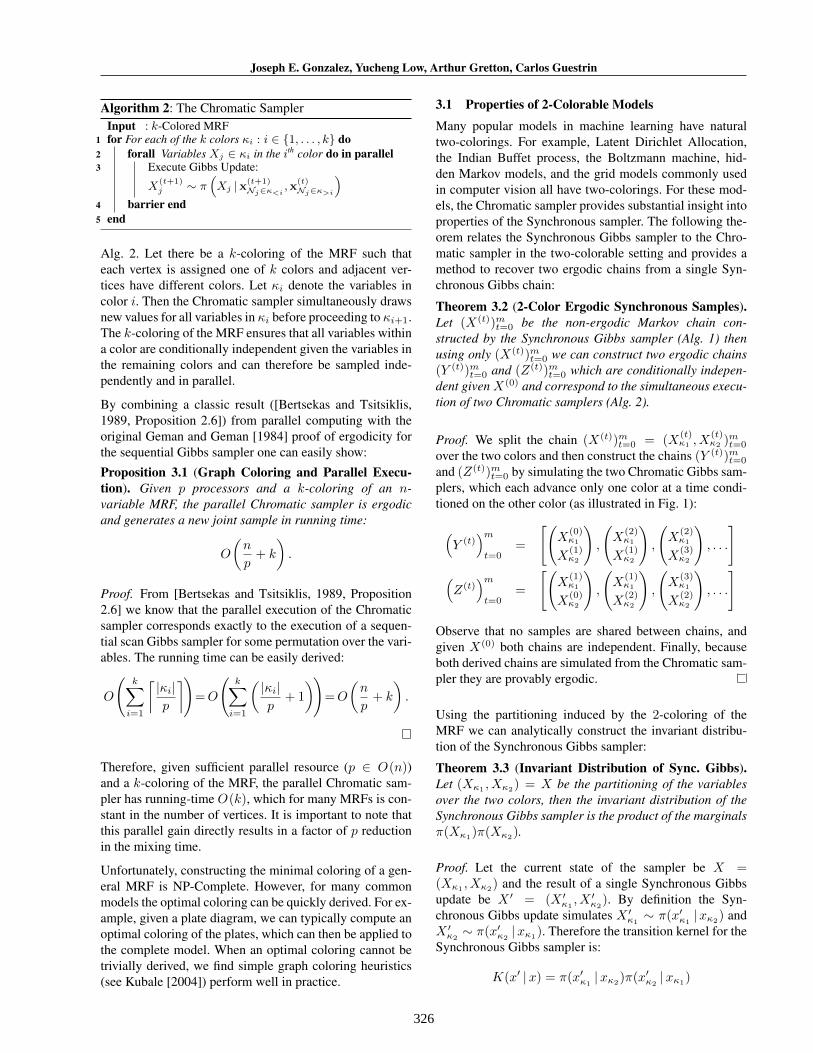
Theorem 3.2 (2-Color Ergodic Synchronous Samples).Let (X(t))mt=0 be the non-ergodic Markov chain con-structed by the Synchronous Gibbs sampler (Alg. 1) thenusing only (X(t))mt=0 we can construct two ergodic chains(Y (t))mt=0 and (Z(t))mt=0 which are conditionally indepen-dent givenX(0) and correspond to the simultaneous execu-tion of two Chromatic samplers (Alg. 2).

Proof. We split the chain (X(t))mt=0 = (X(t)κ1 , X

(t)κ2 )mt=0

over the two colors and then construct the chains (Y (t))mt=0

and (Z(t))mt=0 by simulating the two Chromatic Gibbs sam-plers, which each advance only one color at a time condi-tioned on the other color (as illustrated in Fig. 1):

(Y (t)

)mt=0

=

[(X

(0)κ1

X(1)κ2

),

(X

(2)κ1

X(1)κ2

),

(X

(2)κ1

X(3)κ2

), . . .

](Z(t)

)mt=0

=

[(X

(1)κ1

X(0)κ2

),

(X

(1)κ1

X(2)κ2

),

(X

(3)κ1

X(2)κ2

), . . .

]

Observe that no samples are shared between chains, andgiven X(0) both chains are independent. Finally, becauseboth derived chains are simulated from the Chromatic sam-pler they are provably ergodic.

Using the partitioning induced by the 2-coloring of theMRF we can analytically construct the invariant distribu-tion of the Synchronous Gibbs sampler:

Theorem 3.3 (Invariant Distribution of Sync. Gibbs).Let (Xκ1 , Xκ2) = X be the partitioning of the variablesover the two colors, then the invariant distribution of theSynchronous Gibbs sampler is the product of the marginalsπ(Xκ1

)π(Xκ2).

Proof. Let the current state of the sampler be X =(Xκ1 , Xκ2) and the result of a single Synchronous Gibbsupdate be X ′ = (X ′κ1

, X ′κ2). By definition the Syn-

chronous Gibbs update simulates X ′κ1∼ π(x′κ1

|xκ2) and

X ′κ2∼ π(x′κ2

|xκ1). Therefore the transition kernel for the

Synchronous Gibbs sampler is:

K(x′ |x) = π(x′κ1|xκ2

)π(x′κ2|xκ1

)

327


x1(0)

x2(0)

x1(1)

x2(1)

x1(2)

x2(2)

x1(3)

x2(3)

(a) Synchronous Chain

x1(0) x1

(0)

x2(1)x2

(0) x2(0)

x1(1) x1

(2)

x2(1)x2

(2)

x1(1) x1

(2)

x2(3)x2

(2)

x1(3)

Ergodic Chain 1 Ergodic Chain 2

(b) Two Ergodic Chains

Figure 1: (a) Execution of a two colored model using the synchronous Gibbs sampler. The dotted lines represent dependencies betweensamples. (b) Two ergodic chains obtained by executing the Synchronous Gibbs sampler. Note that ergodic sums with respect to marginalsare equivalent to those obtained using the Synchronous sampler.

We can easily show that π(Xκ1)π(Xκ2

) is the invariant dis-tribution of the Synchronous Gibbs sampler:

P (x′) =∑x

K(x′ |x)π(x)

=∑xκ1

∑xκ2

π(x′κ1|xκ2

)π(x′κ2|xκ1

)π(xκ1)π(xκ2

)

=∑xκ1

∑xκ2

π(xκ1, x′κ2

)π(x′κ1, xκ2

)

= π(x′κ1)π(x′κ2

)

A useful consequence of Theorem 3.3 is that when comput-ing ergodic averages over sets of variables with the samecolor, we can directly use the non-ergodic Synchronoussamples and still obtain convergent estimators:

Corollary 3.4 (Monochromatic Marginal Ergodicity).Given a sequence of samples (x(t))mt=0 drawn from theSynchronous Gibbs sampler on two-colorable model, em-pirical expectations computed with respect to single colormarginals are ergodic:

∀f, i ∈ 1, 2 : limm→∞

1

m

m∑t=0

f(x(t)κi )a.s.−−→ Eπ [f(Xκi)]

Corollary 3.4 therefore justifies many applications wherethe Synchronous Gibbs sampler is used to estimate sin-gle variables marginals and explains why the SynchronousGibbs sampler performs well in these settings. However,Corollary 3.4 also highlights the danger of computing em-pirical expectations over variables that span both colorswithout splitting the chains as shown in Theorem 3.2.

We have shown that both the Chromatic sampler and theSynchronous sampler can provide ergodic samples. How-ever the Chromatic sampler is clearly superior when thenumber of processors is less than the half the number ofvertices (p < n/2) since it will advance a single chaintwice as fast as the Synchronous sampler.

4 THE PARALLEL SPLASH SAMPLERThe Chromatic sampler provides a linear speedup forsingle-chain sampling, advancing the Markov chain for ak-colorable model in time O

(np + k

)rather than O(n).

Algorithm 3: Parallel Splash SamplerInput: Maximum treewidth wmaxInput: Maximum Splash size hmaxwhile t ≤ ∞ do1

// Make p bounded treewidth Splashes

JSipi=1 ← ParSplash(wmax, hmax, x

(t));33// Calibrate each junction trees

JSipi=1 ← ParCalibrate(x(t), JSi

pi=1);55

// Sample each SplashxSi

pi=1 ← ParSample(JSi

pi=1);77

// Advance the chain

x(t+1) ←xS1 , ..., xS1 , x

(t)

¬⋃pi=1 Si

8

Unfortunately, some models possess strongly correlatedvariables and complex dependencies, which can cause theChromatic sampler to mix prohibitively slowly.

In the single processor setting, a common method to accel-erate a slowly mixing Gibbs sampler is to introduce block-ing updates [Barbu and Zhu, 2005, Jensen and Kong, 1996,Hamze and de Freitas, 2004]. In a blocked Gibbs sam-pler, blocks of strongly coupled random variables are sam-pled jointly conditioned on their combined Markov blan-ket. The blocked Gibbs sampler improves mixing by en-abling strongly coupled variables to update jointly when in-dividual conditional updates would cause the chain to mixtoo slowly.

To improve mixing in the parallel setting we introducethe Splash sampler (Alg. 3), a general purpose blockingsampler. For each joint sample, the Splash sampler ex-ploits parallelism both to construct multiple random blocks,called Splashes, and to accelerate the joint sampling of eachSplash. To ensure each Splash can be safely and efficientlysampled in parallel, we developed a novel Splash genera-tion algorithm which incrementally builds multiple condi-tionally independent bounded treewidth junction trees forevery new sample. In the initial rounds of sampling, theSplash algorithm uses a novel adaptation heuristic whichgroups strongly dependent variables together based on thestate of the chain. Adaptation is then disabled after a finitenumber of rounds to ensure ergodicity.

We present the Splash sampler in three parts. First, wepresent the parallel algorithm used to construct multipleconditionally independent Splashes. Next, we describe theparallel junction tree sampling procedure used to jointlysample all variables in a Splash. Finally, we present our

328


Algorithm 4: ParSplash: Parallel Splash GenerationInput: Maximum treewidth wmaxInput: Maximum Splash size hmaxOutput: Disjoint Splashes S1, . . . ,Spdo in parallel on processor i ∈ 1, . . . , p1

r ← NextRoot(i) // Unique roots33Si ← r // Add r to splash4B ← Nr // Add neighbors to boundary5V ← r ∪ Nr // Visited vertices6JSi ← JunctionTree(r)7while (|Si| < hmax)

∧(|B| > 0) do8

v ← NextVertexToExplore(B)1010MarkovBlanketLock(Xv)11// Check that v and its neighbors Nv

are not in other Splashes.

safe←∣∣∣(v ∪ Nv) ∩ (⋃j 6=i Sj)∣∣∣ = 012

JSi+v ← ExtendJunctionTree(JSi , v)13if safe

∧TreeWidth(JSi+v)< wmax then14

JSi ← JSi+v // Accept new tree15Si ← Si ∪ v16B ← B ∪ (Nv\V) // Extend boundary1818V ← V ∪Nv // Mark visited19

MarkovBlanketFree(Xv)20

Splash adaptation heuristic which sets the priorities usedduring Splash generation.

4.1 Parallel Splash Generation

The Splash generation algorithm (Alg. 4) uses p processorsto incrementally build p disjoint Splashes in parallel. Eachprocessor grows a Splash rooted at a unique vertex in theMRF (Line 3). To preserve ergodicity we require that notwo roots share a common edge in the MRF, and that everyvariable is a root infinitely often.

Each Splash is grown incrementally using a best firstsearch (BeFS) of the MRF. The exact order in whichvariables are explored is determined by the call toNextVertexToExplore(B) on Line 10 of Alg. 4which selects (and removes) the next vertex from theboundary B. In Fig. 2 we plot several simultaneousSplashes constructed using a first-in first-out (FIFO) order-ing (Fig. 2(b)) and a prioritized ordering (Fig. 2(d)).

The Splash boundary is extended until there are no remain-ing variables that can be safely added or the Splash is suffi-ciently large. A variable cannot be safely added to a Splashif sampling the resulting Splash is excessively costly (vi-olates a treewidth bound) or if the variable or any of itsneighbors are members of other Splashes (violates condi-tional independence of Splashes).

To bound the computational complexity of sampling, andlater to jointly sample the Splash, we rely on junction trees.A junction tree, or clique graph, is an undirected acyclicgraphical representation of the joint distribution over a col-lection of random variables. For a Splash containing thevariables XS , we construct a junction tree (C, E) = JS

Algorithm 5: ExtendJunctionTree AlgorithmInput: The original junction tree (C, E) = JS .Input: The variable Xi to add to JSOutput: JS+i

Define : Cu as the clique created by eliminating u ∈ SDefine : V[C] ∈ S as the variable eliminated when creating CDefine : t[v] as the time v ∈ S was added to SDefine : P[v] ∈ Nv ∩ S as the next neighbor of v to be

eliminated.Ci ← (Ni ∩ S) ∪ i1P[i]← argmaxv∈Ci\i t[v]2// ----------- Repair RIP -------------R← Ci\ i // RIP Set3v ← P[i]4while |R| > 0 do5

Cv ← Cv ∪R // Add variables to parent6w ← argmaxw∈Cv\v t[w] // Find new parent7if w = P[v] then8R ← (R\Ci)\ i9

else10R ← (R∪ Ci)\ i11P[v]← w // New parent12

v ← P[v] // Move upwards13

representing the conditional distribution π(XS |x−S). Thevertices C ∈ C are often called cliques and represent a sub-set of the indices (i.e., C ⊆ S) in the Splash S. The cliquessatisfy the constraint that for every factor domain A ∈ Fthere exists a clique C ∈ C such that A∩S ⊆ C. The edgesE of the junction tree satisfy the running intersection prop-erty (RIP) which ensures that all cliques sharing a commonvariable form a connected tree.

The computational complexity of a inference, and conse-quently sampling in a junction tree, is exponential in thetreewidth; one less than number of variables in the largestclique. Therefore, to evaluate the computational cost ofadding a new variable Xv to the Splash, we need an effi-cient method to extend the junction tree JS over XS to ajunction tree JS+v over XS∪v and evaluate the resultingtreewidth.

To efficiently build incremental junction trees, we devel-oped a novel junction tree extension algorithm (Alg. 5)which emulates standard variable elimination, with vari-ables being eliminated in the reverse of the order they areadded to the Splash (e.g., if Xi is added to JS then Xi

is eliminated before all XS ). Because each Splash growsoutwards from the root, the resulting elimination orderingis optimal on tree MRFs and typically performs well oncyclic MRFs.

The incremental junction tree extension algorithm (Alg. 5)begins by eliminating Xi and forming the new clique Ci =(Ni ∩ S) ∪ i which is added JS+i. We then attach Cito the most recently added clique CP[i] which contains avariable in Ci (CP[i] denotes the parent of Ci). We thenrestore the RIP by propagating the newly added variablesback up the tree. LettingR = Ci\ i, we insertR into its

329


(a) Noisy (b) FIFO Splashes (c) FIFO Splashes (+) (d) Priority Splashes (e) Priority Splashes (+)

Figure 2: Different Splashes constructed on a 200 × 200 image denoising grid MRF. (a) A noisy sunset image. Eight Splashes oftreewidth 5 were constructed using the FIFO (b) and priority (d) ordering. Each splash is shown in a different shade of gray and theblack pixels are not assigned to any Splash. The priorities were obtained using the adaptive heuristic. In (c) and (e) we zoom in on theSplashes to illustrate their structure and the black pixels along the boundary needed to maintain conditional independence.

56 124 245 45 4

2

4 5

1

6

3

1256 1245 245 45 4 1236

Figure 3: Incremental Junction Tree Example: The junctiontree on the top comprises the subset of variables 1,2,4,5,6 ofthe MRF (center). The tree is formed by the variable eliminationordering 6,1,2,5,4 (reading the underlined variables of the treein reverse). To perform an incremental insertion of variable 3, wefirst create the clique formed by the elimination of 3 (1,2,3,6)and insert it into the end of the tree. Its parent is set to the latestoccurrence of any of the variables in the new clique. Next theset 1,2,6 is inserted into its parent (boldface variables), and itsparent is recomputed in the same way.

parent clique CP[i]. The RIP condition is now satisfied forvariables in R which were already in CP[i]. The parent forCP[i] is then recomputed, and any unsatisfied variables arepropagated up the tree in the same way. We demonstratethis algorithm with a simple example in Fig. 3.

To ensure that simultaneously constructed Splashes areconditionally independent, we develop the Markov blanketlocking (MBL) protocol which associates a lock with eachvariable in the model. The Markov blanket lock for variableXv is obtained by acquiring the read-locks on all neighbor-ing variables XNv and the write lock on Xv . Locks are ac-quired and released using a canonical ordering of the vari-ables to prevent deadlocks.

Once the MarkovBlanketLock(Xv) has been ac-quired, no other processor can assignXv or any of it neigh-bors XNv to a Splash. Therefore, we can safely test ifXv or any of its neighbors XNv are currently assignedto other Splashes. Since we only add Xv to the Splash ifboth Xv and all its neighbors are currently unassigned toother Splashes, there will never be an edge in the MRF thatconnects two Splashes. Consequently, simultaneously con-structed Splashes are conditionally independent given allremaining unassigned variables.

4.2 Parallel Splash SamplingOnce we have constructed p conditionally independentSplashes S1pi=1, we jointly sample each Splash by draw-ing from π(XSi |x−Si) in parallel. This is accomplished bycalibrating the junction trees JSi

pi=1, and then running

backward-sampling starting at the root to jointly sampleall the variables in each Splash. We also use the calibratedjunction trees to construct Rao-Blackwellized marginal es-timators. If the treewidth or the size of each Splash is large,it may be beneficial to construct fewer Splashes, and in-stead assign multiple processors to accelerate the calibra-tion and sampling of individual junction trees.

To calibrate the junction tree we use the ParCalibratefunction. The ParCalibrate function constructs allclique potentials in parallel by computing the products ofthe assigned factors conditioned on the variables not in theSplash. Finally, parallel belief propagation is used to cali-brate the tree by propagating messages in parallel followingthe optimal forward-backward schedule.

Parallel backward-sampling is accomplished by the func-tion ParSample which takes the calibrated junctiontree and draws a new joint assignment in parallel. TheParSample function begins by drawing a new joint as-signment for the root clique using the calibrated marginal.Then in parallel each child is sampled conditioned on theparent assignment and the messages from the children.

4.3 Adaptive Splash GenerationAs discussed earlier, the order in which variables are ex-plored when constructing a Splash is determined on Line 10in the ParSplash algorithm (Alg. 4). We propose a sim-ple adaptive prioritization heuristic, based on the currentassignment to x(t), that prioritizes variables at the bound-ary of the current tree which are strongly coupled withvariables already in the Splash. We assign each variableXv ∈ B a score using the likelihood ratio:

s[Xv] =

∣∣∣∣∣∣∣∣∣∣∣∣log

∑x π(XS , Xv = x |X−S = x

(t)−S

)π(XS , Xv = x

(t)v |X−S = x

(t)−S

)∣∣∣∣∣∣∣∣∣∣∣∣1

,

(4.1)

330


(a) Early (b) Later

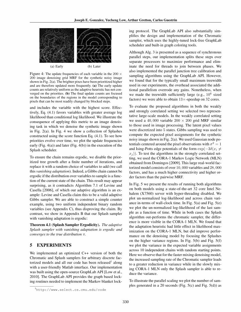
Figure 4: The update frequencies of each variable in the 200 ×200 image denoising grid MRF for the synthetic noisy imageshown in Fig. 2(a). The brighter pixes have been prioritized higherand are therefore updated more frequently. (a) The early updatecounts are relatively uniform as the adaptive heuristic has not con-verged on the priorities. (b) The final update counts are focusedon the boundaries of the regions in the model corresponding topixels that can be most readily changed by blocked steps.

and includes the variable with the highest score. Effec-tively, Eq. (4.1) favors variables with greater average loglikelihood than conditional log likelihood. We illustrate theconsequence of applying this metric to an image denois-ing task in which we denoise the synthetic image shownin Fig. 2(a). In Fig. 4 we show a collection of Splashesconstructed using the score function Eq. (4.1). To see howpriorities evolve over time, we plot the update frequenciesearly (Fig. 4(a)) and later (Fig. 4(b)) in the execution of theSplash scheduler.

To ensure the chain remains ergodic, we disable the prior-itized tree growth after a finite number of iterations, andreplace it with a random choice of variables to add (we callthis vanishing adaptation). Indeed, a Gibbs chain cannot beergodic if the distribution over variables to sample is a func-tion of the current state of the chain. This result may appearsurprising, as it contradicts Algorithm 7.1 of Levine andCasella [2006], of which our adaptive algorithm is an ex-ample: Levine and Casella claim this to be a valid adaptiveGibbs sampler. We are able to construct a simple counterexample, using two uniform independent binary randomvariables (see Appendix C), thus disproving the claim. Bycontrast, we show in Appendix B that our Splash samplerwith vanishing adaptation is ergodic:

Theorem 4.1 (Splash Sampler Ergodicity). The adaptiveSplash sampler with vanishing adaptation is ergodic andconverges to the true distribution π.

5 EXPERIMENTS

We implemented an optimized C++ version of both theChromatic and Splash samplers for arbitrary discrete fac-torized models and all our code has been released1 alongwith a user-friendly Matlab interface. Our implementationwas built using the open-source GraphLab API [Low et al.,2010]. The GraphLab API provides the graph based lock-ing routines needed to implement the Markov blanket lock-

1http://www.select.cs.cmu.edu/code

ing protocol. The GraphLab API also substantially sim-plifies the design and implementation of the Chromaticsampler, which uses the highly-tuned lock-free GraphLabscheduler and built-in graph coloring tools.

Although Alg. 3 is presented as a sequence of synchronousparallel steps, our implementation splits these steps overseparate processors to maximize performance and elim-inate the need for threads to join between phases. Wealso implemented the parallel junction tree calibration andsampling algorithms using the GraphLab API. However,we found that for the typically small maximum treewidthused in our experiments, the overhead associated the addi-tional parallelism overrode any gains. Nonetheless, whenwe made the treewidth sufficiently large (e.g., 106 sizedfactors) we were able to obtain 13×-speedup on 32 cores.

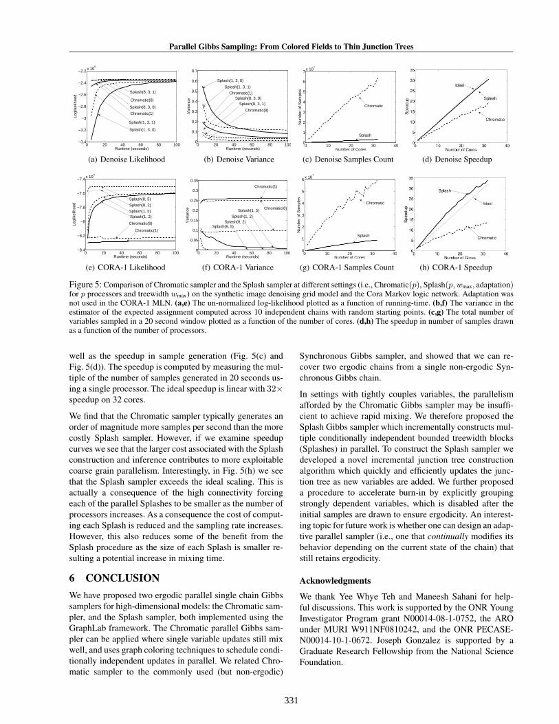
To evaluate the proposed algorithms in both the weaklyand strongly correlated setting we selected two represen-tative large-scale models. In the weakly correlated settingwe used a 40, 000 variable 200 × 200 grid MRF similarto those used in image processing. The latent pixel valueswere discretized into 5 states. Gibbs sampling was used tocompute the expected pixel assignments for the syntheticnoisy image shown in Fig. 2(a). We used Gaussian node po-tentials centered around the pixel observations with σ2 = 1and Ising-Potts edge potentials of the form exp(−3δ(xi 6=xj)). To test the algorithms in the strongly correlated set-ting, we used the CORA-1 Markov Logic Network (MLN)obtained from Domingos [2009]. This large real-world fac-torized model consists of over 10, 000 variables and 28, 000factors, and has a much higher connectivity and higher or-der factors than the pairwise MRF.

In Fig. 5 we present the results of running both algorithmson both models using a state-of-the-art 32 core Intel Ne-halem (X7560) server with hyper-threading disabled. Weplot un-normalized log-likelihood and across chain vari-ance in-terms of wall-clock time. In Fig. 5(a) and Fig. 5(e)we plot the un-normalized log-likelihood of the last sam-ple as a function of time. While in both cases the Splashalgorithm out-performs the chromatic sampler, the differ-ence is more visible in the CORA-1 MLN. We found thatthe adaptation heuristic had little effect in likelihood max-imization on the CORA-1 MLN, but did improve perfor-mance on the denoising model by focusing the Splasheson the higher variance regions. In Fig. 5(b) and Fig. 5(f)we plot the variance in the expected variable assignmentsacross 10 independent chains with random starting points.Here we observe that for the faster mixing denoising model,the increased sampling rate of the Chromatic sampler leadsto a greater reduction in variance while in the slowly mix-ing CORA-1 MLN only the Splash sampler is able to re-duce the variance.

To illustrate the parallel scaling we plot the number of sam-ples generated in a 20 seconds (Fig. 5(c) and Fig. 5(d)) as

331


0 20 40 60 80 100−3.4

−3.2

−3

−2.8

−2.6

−2.4

−2.2x 10

5

Runtime (seconds)

Logl

ikel

ihoo

d

Splash(8, 3, 1)

Splash(8, 3, 0)

Splash(1, 3, 1)

Splash(1, 3, 0)

Chromatic(8)

Chromatic(1)

(a) Denoise Likelihood

0 20 40 60 80 1000

0.1

0.2

0.3

0.4

0.5

0.6

0.7

Runtime (seconds)

Var

ianc

e Splash(8, 3, 0)Splash(8, 3, 1)

Splash(1, 3, 0)

Splash(1, 3, 1)

Chromatic(1)

Chromatic(8)

(b) Denoise Variance

0 10 20 30 400

1

2

3

4

5

6

7x 10

7

Number of Cores

Num

ber

of S

ampl

es

Chromatic

Splash

(c) Denoise Samples Count (d) Denoise Speedup

0 20 40 60 80 100−8.4

−8.2

−8

−7.8

−7.6

−7.4x 10

4

Runtime (seconds)

Logl

ikel

ihoo

d

Splash(8, 5)

Splash(8, 2)

Splash(1, 5)Splash(1, 2)

Chromatic(8)

Chromatic(1)

(e) CORA-1 Likelihood

0 20 40 60 80 1000

0.05

0.1

0.15

0.2

0.25

0.3

0.35

Runtime (seconds)

Var

ianc

e Splash(1, 5)

Splash(1, 2)Splash(8, 2)

Splash(8, 5)

Chromatic(8)

Chromatic(1)

(f) CORA-1 Variance

0 10 20 30 400

1

2

3

4

5

6x 10

7

Number of Cores

Num

ber

of S

ampl

es

Chromatic

Splash

(g) CORA-1 Samples Count (h) CORA-1 Speedup

Figure 5: Comparison of Chromatic sampler and the Splash sampler at different settings (i.e., Chromatic(p), Splash(p, wmax, adaptation)for p processors and treewidth wmax) on the synthetic image denoising grid model and the Cora Markov logic network. Adaptation wasnot used in the CORA-1 MLN. (a,e) The un-normalized log-likelihood plotted as a function of running-time. (b,f) The variance in theestimator of the expected assignment computed across 10 independent chains with random starting points. (c,g) The total number ofvariables sampled in a 20 second window plotted as a function of the number of cores. (d,h) The speedup in number of samples drawnas a function of the number of processors.

well as the speedup in sample generation (Fig. 5(c) andFig. 5(d)). The speedup is computed by measuring the mul-tiple of the number of samples generated in 20 seconds us-ing a single processor. The ideal speedup is linear with 32×speedup on 32 cores.

We find that the Chromatic sampler typically generates anorder of magnitude more samples per second than the morecostly Splash sampler. However, if we examine speedupcurves we see that the larger cost associated with the Splashconstruction and inference contributes to more exploitablecoarse grain parallelism. Interestingly, in Fig. 5(h) we seethat the Splash sampler exceeds the ideal scaling. This isactually a consequence of the high connectivity forcingeach of the parallel Splashes to be smaller as the number ofprocessors increases. As a consequence the cost of comput-ing each Splash is reduced and the sampling rate increases.However, this also reduces some of the benefit from theSplash procedure as the size of each Splash is smaller re-sulting a potential increase in mixing time.

6 CONCLUSIONWe have proposed two ergodic parallel single chain Gibbssamplers for high-dimensional models: the Chromatic sam-pler, and the Splash sampler, both implemented using theGraphLab framework. The Chromatic parallel Gibbs sam-pler can be applied where single variable updates still mixwell, and uses graph coloring techniques to schedule condi-tionally independent updates in parallel. We related Chro-matic sampler to the commonly used (but non-ergodic)

Synchronous Gibbs sampler, and showed that we can re-cover two ergodic chains from a single non-ergodic Syn-chronous Gibbs chain.

In settings with tightly couples variables, the parallelismafforded by the Chromatic Gibbs sampler may be insuffi-cient to achieve rapid mixing. We therefore proposed theSplash Gibbs sampler which incrementally constructs mul-tiple conditionally independent bounded treewidth blocks(Splashes) in parallel. To construct the Splash sampler wedeveloped a novel incremental junction tree constructionalgorithm which quickly and efficiently updates the junc-tion tree as new variables are added. We further proposeda procedure to accelerate burn-in by explicitly groupingstrongly dependent variables, which is disabled after theinitial samples are drawn to ensure ergodicity. An interest-ing topic for future work is whether one can design an adap-tive parallel sampler (i.e., one that continually modifies itsbehavior depending on the current state of the chain) thatstill retains ergodicity.

Acknowledgments

We thank Yee Whye Teh and Maneesh Sahani for help-ful discussions. This work is supported by the ONR YoungInvestigator Program grant N00014-08-1-0752, the AROunder MURI W911NF0810242, and the ONR PECASE-N00014-10-1-0672. Joseph Gonzalez is supported by aGraduate Research Fellowship from the National ScienceFoundation.

332


ReferencesM. Kuss and C. E. Rasmussen. Assessing approximate inference

for binary gaussian process classification. J. Mach. Learn. Res.,6, 2005.

A. Barbu and S. Zhu. Generalizing swendsen-wang to samplingarbitrary posterior probabilities. IEEE Trans. Pattern Anal.Mach. Intell., 27(8), 2005.

F. Doshi-Velez, D. Knowles, S. Mohamed, and Z. Ghahramani.Large scale nonparametric bayesian inference: Data paralleli-sation in the indian buffet process. In NIPS 22, 2009.

D. Newman, A. Asuncion, P. Smyth, and M. Welling. Distributedinference for latent dirichlet allocation. In NIPS, 2007.

A. Asuncion, P. Smyth, and M. Welling. Asynchronous dis-tributed learning of topic models. In NIPS, 2008.

F. Yan, N. Xu, and Y. Qi. Parallel inference for latent dirichletallocation on graphics processing units. In NIPS, 2009.

C. S. Jensen and A. Kong. Blocking gibbs sampling for linkageanalysis in large pedigrees with many loops. In American Jour-nal of Human Genetics, 1996.

Y. Low, J. Gonzalez, A. Kyrola, D. Bickson, C. Guestrin, andJ. Hellerstein. Graphlab: A new framework for parallel ma-chine learning. In UAI, 2010.

S. Geman and D. Geman. Stochastic relaxation, gibbs distribu-tions, and the bayesian restoration of images. In PAMI, 1984.

P. A. Ferrari, A. Frigessi, and R. H. Schonmann. Convergenceof some partially parallel gibbs samplers with annealing. TheAnnals of Applied Probability, 3(1), 1993.

D. Bertsekas and J. Tsitsiklis. Parallel and Distributed Computa-tion: Numerical Methods. Athena Scientific, 1989.

M. Kubale. Graph Colorings. American Mathematical Society,2004.

F. Hamze and N. de Freitas. From fields to trees. In UAI, 2004.

R. A. Levine and G. Casella. Optimizing random scan gibbs sam-plers. J. Multivar. Anal., 97(10), 2006.

P. Domingos. Uw-cse mlns, 2009. URL alchemy.cs.washington.edu/mlns/cora.

parallel gibbs sampling: from colored fields to thin junction

Documents