parallel magnetic resonance...
TRANSCRIPT
IOP PUBLISHING PHYSICS IN MEDICINE AND BIOLOGY
Phys. Med. Biol. 52 (2007) R15–R55 doi:10.1088/0031-9155/52/7/R01
INVITED TOPICAL REVIEW
Parallel magnetic resonance imaging
David J Larkman and Rita G Nunes
The Imaging Sciences Department, Clinical Sciences Centre, Faculty of Medicine,Imperial College London, Hammersmith Hospital Campus, Du Cane Road, LondonW12 0NN, UK
E-mail: [email protected]
Received 30 December 2005, in final form 9 February 2007Published 9 March 2007Online at stacks.iop.org/PMB/52/R15
AbstractParallel imaging has been the single biggest innovation in magnetic resonanceimaging in the last decade. The use of multiple receiver coils to augment thetime consuming Fourier encoding has reduced acquisition times significantly.This increase in speed comes at a time when other approaches to acquisitiontime reduction were reaching engineering and human limits. A brief summaryof spatial encoding in MRI is followed by an introduction to the problem parallelimaging is designed to solve. There are a large number of parallel reconstructionalgorithms; this article reviews a cross-section, SENSE, SMASH, g-SMASHand GRAPPA, selected to demonstrate the different approaches. Theoretical(the g-factor) and practical (coil design) limits to acquisition speed are reviewed.The practical implementation of parallel imaging is also discussed, in particularcoil calibration. How to recognize potential failure modes and their associatedartefacts are shown. Well-established applications including angiography,cardiac imaging and applications using echo planar imaging are reviewed andwe discuss what makes a good application for parallel imaging. Finally, activeresearch areas where parallel imaging is being used to improve data quality byrepairing artefacted images are also reviewed.
(Some figures in this article are in colour only in the electronic version)
1. Introduction and background
Parallel imaging (PI) or partially parallel imaging (PPI) has in the last few years translatedfrom a research topic to a widely used commercial product with significant impact on almostevery facet of practice of magnetic resonance imaging (MRI). PI makes use of spatiallyseparated receiver antennas to perform some of the spatial encoding required to turn thenuclear magnetic resonance (NMR) phenomena into magnetic resonance imaging (MRI). PI’shistory is an interesting one, the theoretical foundations were laid in the late 1980s, but itlay dormant for more than a decade, partly because appropriate hardware was not readily
0031-9155/07/070015+41$30.00 © 2007 IOP Publishing Ltd Printed in the UK R15
R16 Invited Topical Review
available and partly because whilst array coils had been developed, they were being usedin a different way; to provide high signal-to-noise ratio (SNR), large field of view (FOV)images. The second wave of research interest in PI came in the late 1990s and within 5 yearswas widely commercialized. However, the field is still an active area of research in its ownright, maintaining a rapid pace of development in both concepts and applications. The fieldhas drawn on many different aspects of hardware engineering and mathematics to improveand expand the original concepts and to use the technology to help tackle many of the majorproblems which exist in MRI.
1.1. Spatial encoding in MRI
To put PI in context and to enable the reader to appreciate the necessity of its development, weneed first describe how spatial encoding in MRI is performed in the absence of PI and introducesome terminology. MRI is not actually an imaging method as it would be defined by imagingphysics. The image is formed by localizing the NMR signal by frequency. This frequencydependent localization makes MRI a spectroscopic technique. The localization concept isstraightforward. The resonant frequency of the nuclear spin system is defined by the Larmorequation (equation (1)) where ω is the resonant frequency and γ the gyromagnetic ratio of theproton (42.58 MHz T−1), B is the external magnetic field strength at the proton position, andso ω is directly proportional to the strength of the external magnetic field experienced by thespin system:
ω = γB. (1)
The magnitude of the signal is dictated in part by the degree of polarization of the spin systemwhich is also proportional to the magnitude of the main magnetic field and also by the time atwhich the system is measured after perturbation with an RF pulse. This is due to the relaxationof the spin system back to its thermal equilibrium state. The governing equations for such asystem are the Bloch equations which can be simplified for a simple MRI experiment to:
S = S0(1 − e− T R
T 1)
e− T ET 2 (2)
where S is the signal detected, S0 is the maximum detectable signal, proportional to B andto the density of protons (or spins), and the exponential terms describe both the transverseand the longitudinal components of the magnetization as a function of time. This leads totwo key MRI parameters, the echo time (TE), time between excitation and detection andthe repeat time (TR) time between one excitation and the next. For a full description of thegoverning principles and equations of MRI we suggest the book reference (Haacke et al 1999).Equation (2) explains why there is a drive to ever higher main magnetic field strengths in MRIto increase S0, while in equation (1) the dependence of the resonance frequency on B indicatesthe spatial localization mechanism which we will now describe briefly.
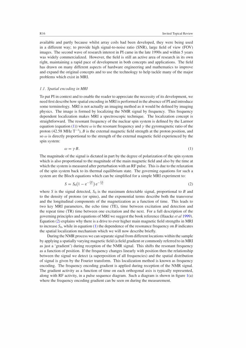
During the NMR process we can separate signal from different locations within the sampleby applying a spatially varying magnetic field (a field gradient or commonly referred to in MRIas just a ‘gradient’) during reception of the NMR signal. This shifts the resonant frequencyas a function of position. If the frequency changes linearly with position then the relationshipbetween the signal we detect (a superposition of all frequencies) and the spatial distributionof signal is given by the Fourier transform. This localization method is known as frequencyencoding. The frequency encoding gradient is applied during reception of the NMR signal.The gradient activity as a function of time on each orthogonal axis is typically represented,along with RF activity, in a pulse sequence diagram. Such a diagram is shown in figure 1(a)where the frequency encoding gradient can be seen on during the measurement.
Invited Topical Review R17
Figure 1. On the left-hand side is a pulse sequence diagram which describes the sequence ofevents on the three orthogonal gradient axes, the RF excitation and the acquisition window. Thefirst action is the RF excitation along with a slice selecting gradient followed by its refocusinggradient. The next step is phase encoding and readout pre-phasing gradient. Finally the readout(frequency encoding) gradient is applied while the signal is collected. In order to fully encodean image, this sequence is repeated for different amplitudes of the phase encode gradient. Theright-hand side shows a schematic representation of k-space. When the phase encode gradient iszero the pre-winding gradient takes us to the left of k-space and the readout gradient sweeps acrossk-space. When a phase encode gradient is applied, it shifts the readout line in k-space along thephase encode direction by an amount �k. The magnitude of �k is inversely proportional to thefield of view (FOV) and the maximum extent of k-space is inversely proportional to the voxel size.
In MRI we generally do not collect data immediately after the RF pulse as we needtime to perform spatial encoding (to play out further gradients) in the orthogonal direction tofrequency encoding before data collection. A full description of this process can be found inHaacke et al (1999).
Frequency encoding can localize signal in one dimension but for imaging a volumewe need 3D localization or 2D localization combined with slice selection to image a plane.The distinction between 3D and multi-slice will be made later, here we will just consider singleslice imaging (which is easily generalizable to multi-slice as this is simply a repetition of thesame scheme at different locations in the magnet). Slice selection is achieved by applying astrong linear gradient in the slice direction (orthogonal to the imaging plane) during excitation,i.e. the delivery of the RF pulse. When a slice select gradient is applied, the Larmor frequencychanges as a function of position and as the RF pulse has a finite bandwidth, only the positionswithin the body for which the Larmor frequency is within the bandwidth of the pulse areexcited, while the spins located in regions corresponding to a frequency outside this rangeare not affected. Figure 1(a) shows the slice selection gradient being activated during the RFpulse.
For this review it is localization along the other in-plane direction that is of most interestas this is where MRI becomes time consuming. In effect the same principle is used asin frequency encoding but encoding along the two directions must be done sequentially assuperimposed gradients suffer from non-unique spatial frequency allocation. This sequentialrequirement imposes a significant time penalty. Frequency encoding can only be performedduring the sampling period and so encoding in the other direction must be done by a methodthat has become known as phase encoding. A gradient is switched on for a period of time, sothat phase is accumulated in the sample as a function of position in space. After some time thisgradient is switched off and the signal is sampled. The effect of the phase encoding gradientis to select a single spatial frequency in the phase encode direction. To sample all requiredspatial frequencies needed to reconstruct an image of the required fidelity the experiment mustbe repeated until all spatial frequencies are sampled, i.e. repeated experiments with varying
R18 Invited Topical Review
phase encode gradients. To give a feeling for the time this process takes, consider that wemay typically use a repeat time of several hundred milliseconds, and hence if a final imageresolution of 256 samples in the frequency encode direction and 256 phase encodes is requiredthen the total imaging time may be several minutes. Imaging times of this length have obviousimplications. The subject is liable to move during imaging causing artefacts in the images,and dynamic processes changing on a time scale shorter than this are difficult to capture.We have now described most of the features of figure 1(a) covering the essential elements ofthe simplest MR imaging sequence, the gradient recalled echo sequence (GRE). For a fullerdescription of pulse sequences we again suggest reference book (Haacke et al 1999).
So far the discussion has been limited to single- or multi-slice imaging, however volumeencoding is also often used in MRI. Here we do not excite a single slice but a larger volume(which can be considered a fat slice) and then spatially encode along the width of the slice usinga second direction of phase encoding, so that now we have two orthogonal directions of phaseencoding. 3D encoding has advantages over multi-slice encoding in both SNR (enhanced byadditional Fourier averaging) and enabling isotropic resolution.
Because image information is not encoded directly, but is encoded in frequency space,we refer to this native data domain as k-space (the k is by analogy to wave-number). This isa reciprocal domain and it is related to the image domain by a 2D or 3D Fourier transform,which naturally translates from the time domain in which we measure (time evolves duringthe sampling of the echo and a pseudo-time evolves during phase encoding) to the frequencydomain (which in MRI is our image domain). The effects of gradients are best described ink-space where we can see that the readout gradient (or frequency encode gradient) allows usto sample along a line in k-space (from negative to positive values due to echo formation),while the phase encode gradient allows us to position this line in the orthogonal direction ink-space (figure 1(b)).
1.2. k-space
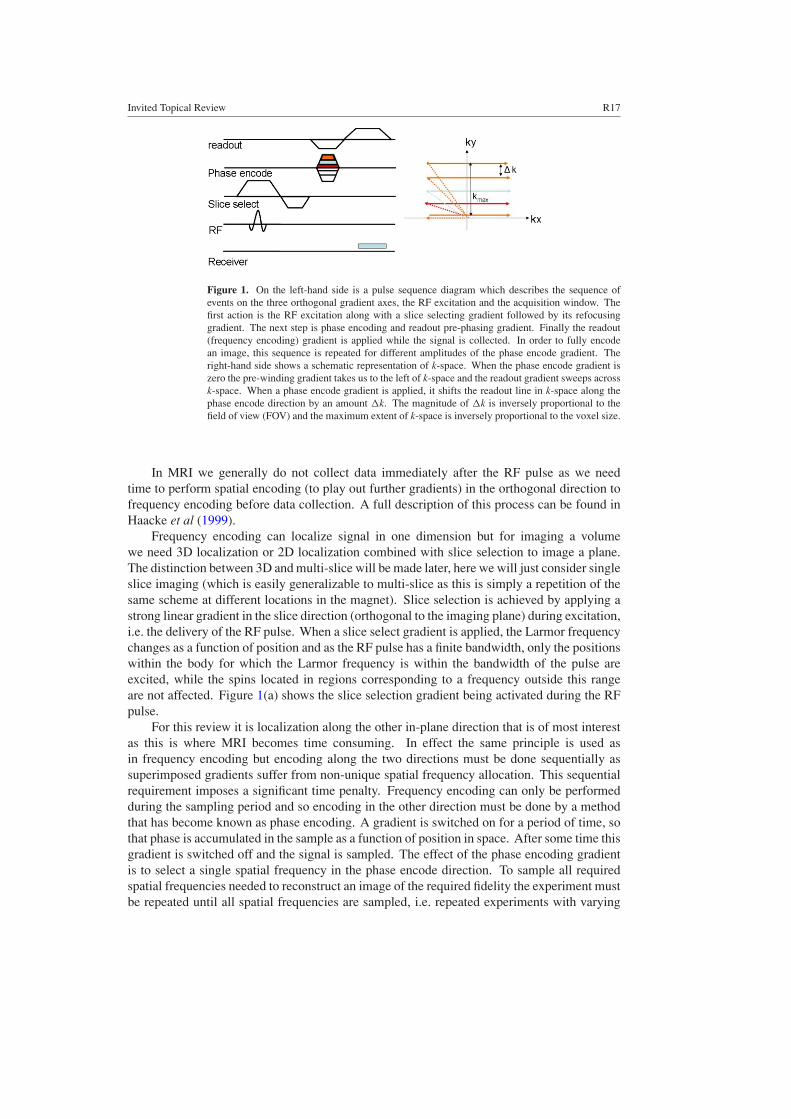
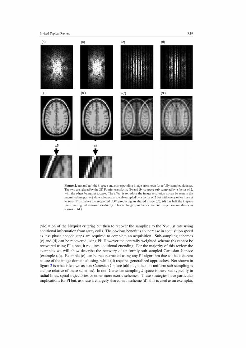
The resolution of the final image is determined by the highest spatial frequency sampled (theextent over which k-space is sampled), kmax, while the field of view is dictated by the frequencyrange we can sample and so is determined by the sampling rate �k (see figure 1(b)). k-spaceis discreetly sampled. In the frequency encode direction the sampling rate is limited by theanalogue-to-digital converter (ADC) used on the receiver boards of the scanner. Typicallythis sampling rate is high and so we rarely need to consider the usual limitations of discretesampling (aliasing etc) in this direction. However, in the phase encode direction the samplingrate is dictated by the magnitude of the k-space shift imposed by the phase encode gradientlobe. As each phase encoding step takes a significant amount of time, it is beneficial tominimize the number of steps required to traverse a fixed extent of k-space (to maintain a fixedresolution). This drives us to take as large a step in k-space as possible, i.e. as small a field ofview as possible. However, if a field of view is chosen which does not wholly contain the objectto be imaged, then this discrete sampling results in aliasing (a consequence of violation of theNyquist criteria in sampling). In the image this manifests itself as the parts of the object whichfall outside the field of view set by the phase encode sampling interval ‘wrapping’ into theimage. Figure 2 shows the effect of three different k-space sampling strategies where (a) showsthe fully sampled k-space, while (b), (c) and (d) have half the number of samples and thereforetook half as long to acquire. The 2D Fourier transforms of (a), (b), (c) and (d) are shown in(a′), (b′), (c′) and (d′) respectively. In (b) the resolution was reduced (kmax reduced) while in(c) the FOV was reduced to half, in (d) a random sub-sampling of k-space was performed. Therole of parallel imaging in its simplest form is to allow larger sampling intervals in k-space
Invited Topical Review R19
(a) (b) (c) (d)
(a,) (b
,) (c
,) (d
,)
x5 x5
Figure 2. (a) and (a′) the k-space and corresponding image are shown for a fully sampled data set.The two are related by the 2D Fourier transform; (b) and (b′) k-space sub-sampled by a factor of 2,with the edges being set to zero. The effect is to reduce the image resolution as can be seen in themagnified images; (c) shows k-space also sub-sampled by a factor of 2 but with every other line setto zero. This halves the supported FOV, producing an aliased image (c′); (d) has half the k-spacelines missing but removed randomly. This no longer produces coherent image domain aliases asshown in (d′).
(violation of the Nyquist criteria) but then to recover the sampling to the Nyquist rate usingadditional information from array coils. The obvious benefit is an increase in acquisition speedas less phase encode steps are required to complete an acquisition. Sub-sampling schemes(c) and (d) can be recovered using PI. However the centrally weighted scheme (b) cannot berecovered using PI alone, it requires additional encoding. For the majority of this review theexamples we will show describe the recovery of uniformly sub-sampled Cartesian k-space(example (c)). Example (c) can be reconstructed using any PI algorithm due to the coherentnature of the image domain aliasing, while (d) requires generalized approaches. Not shown infigure 2 is what is known as non-Cartesian k-space (although the non-uniform sub-sampling isa close relative of these schemes). In non-Cartesian sampling k-space is traversed typically inradial lines, spiral trajectories or other more exotic schemes. These strategies have particularimplications for PI but, as these are largely shared with scheme (d), this is used as an exemplar.
R20 Invited Topical Review
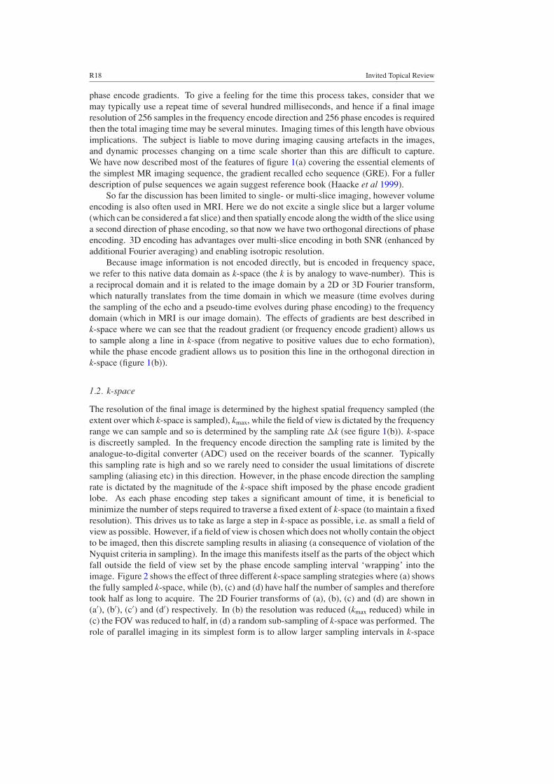
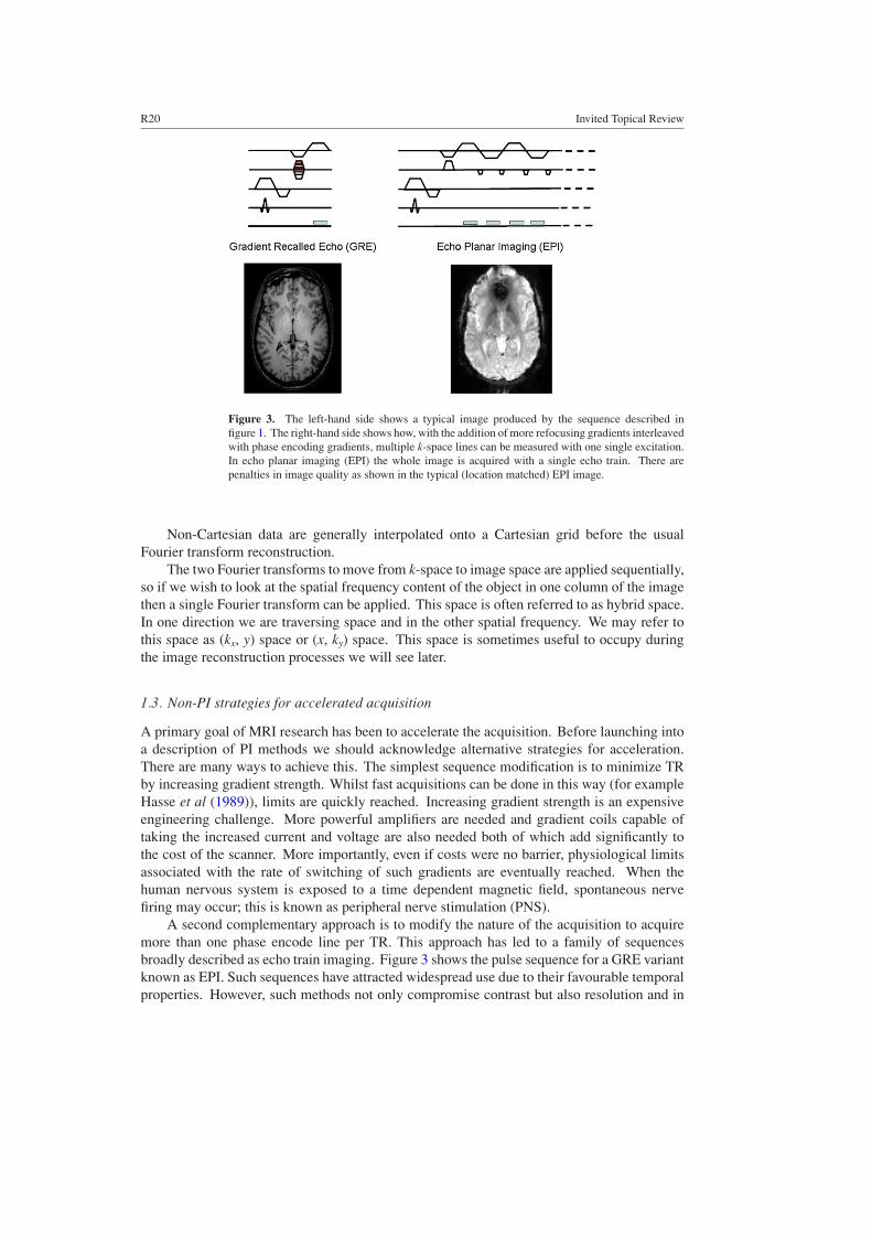
Figure 3. The left-hand side shows a typical image produced by the sequence described infigure 1. The right-hand side shows how, with the addition of more refocusing gradients interleavedwith phase encoding gradients, multiple k-space lines can be measured with one single excitation.In echo planar imaging (EPI) the whole image is acquired with a single echo train. There arepenalties in image quality as shown in the typical (location matched) EPI image.
Non-Cartesian data are generally interpolated onto a Cartesian grid before the usualFourier transform reconstruction.
The two Fourier transforms to move from k-space to image space are applied sequentially,so if we wish to look at the spatial frequency content of the object in one column of the imagethen a single Fourier transform can be applied. This space is often referred to as hybrid space.In one direction we are traversing space and in the other spatial frequency. We may refer tothis space as (kx, y) space or (x, ky) space. This space is sometimes useful to occupy duringthe image reconstruction processes we will see later.
1.3. Non-PI strategies for accelerated acquisition
A primary goal of MRI research has been to accelerate the acquisition. Before launching intoa description of PI methods we should acknowledge alternative strategies for acceleration.There are many ways to achieve this. The simplest sequence modification is to minimize TRby increasing gradient strength. Whilst fast acquisitions can be done in this way (for exampleHasse et al (1989)), limits are quickly reached. Increasing gradient strength is an expensiveengineering challenge. More powerful amplifiers are needed and gradient coils capable oftaking the increased current and voltage are also needed both of which add significantly tothe cost of the scanner. More importantly, even if costs were no barrier, physiological limitsassociated with the rate of switching of such gradients are eventually reached. When thehuman nervous system is exposed to a time dependent magnetic field, spontaneous nervefiring may occur; this is known as peripheral nerve stimulation (PNS).
A second complementary approach is to modify the nature of the acquisition to acquiremore than one phase encode line per TR. This approach has led to a family of sequencesbroadly described as echo train imaging. Figure 3 shows the pulse sequence for a GRE variantknown as EPI. Such sequences have attracted widespread use due to their favourable temporalproperties. However, such methods not only compromise contrast but also resolution and in

Invited Topical Review R21
some cases lead to image distortion; the example images in figure 3 demonstrate the loss inquality between GRE and EPI images. These image artefacts can all be reduced significantlyby reducing the number of echoes in the echo train, an important observation we will returnto in the PI applications section.
Another strategy is to localize the region of excitation which will enable reduction of thefield of view without aliasing. The aliasing seen in figure 2 can be suppressed if only the portionof the object that exists within the reduced field of view is excited. Unfortunately, long pulsetrains are needed and if the pulse length is long compared to the relaxation times of the samplethen the region of excitation will be ill defined. Because of this limit, localized excitation hasremained a niche method. However it is interesting to note that recent developments whichhave spun out of PI, known as parallel transmit (PT) may now be making this possible onrealistic time scales (Katscher et al 2003).
Finally we can replace fully or partially the Fourier encoding with some other basis set:singular value decomposition (SVD) (Zientara et al 1994), wavelet (Panych and Jolesz 1994)or Hadamard (Panych et al 1997) for example. These other basis sets may be able to morecompactly describe the contents of a medical image than a Fourier basis set but these methodsare limited due to the complexities of selecting the appropriate basis set given a target. Again,PI has renewed interest in some of these methods to augment coil encoding, the centrallyweighted sub-sampling scheme shown in figure 2(b) can only be recovered with PI if it isaugmented with another encoding scheme (Kyriakos et al 2006).
A wide range of acquisition methods have been proposed where full k-space is not sampled.These methods differ from PI, where k-space is also undersampled, in that sparse methods aimto exclude redundant data. For example, the theoretical conjugate symmetry of k-space canbe exploited with part of k-space remaining uncollected and then repopulated using variousmethods (Margosian et al 1986). When multiple time point imaging is being performed, forexample to track the effect of a contrast injection, then there have been many proposals forimproving the temporal resolution, most of which are based on updating different parts ofk-space at different frequencies (the centre more often than the edges for example van Vaalset al (1993)). More recently, a new family of acceleration methods for time course data havebeen proposed. These have specific k-space sampling patterns which produce aliases in x–fspace (where x is image domain and f is frequency, the Fourier transform of the time series ofimages). The specific details of the sampling pattern dictate the location of these aliases andprovided there is rapidly changing information only in part of the field of view, the overlapof these aliases can be made very small and highly accurate reconstructions can be performed(Tsao et al 2003, Malik et al 2006).
All these strategies are successful to a greater or lesser degree. All have limits which havealready been met but all can be complemented with coil encoding.
1.4. Why parallel imaging?
If design criteria were written for a method for image acceleration the key features would bethat it:
• is applicable to all pulse sequences without affecting image contrast;• is complementary to all existing acceleration methods;• does not introduce artefacts or adversely affect SNR.
Coil encoding scores full marks on the first two bullet points. The last is a complex pointdeserving of its own section. In general PI does not introduce significant artefacts but it doesreduce SNR and this is its weakness. However, as we will see, the benefits are large and whenapplied intelligently far outweigh this limitation.
R22 Invited Topical Review
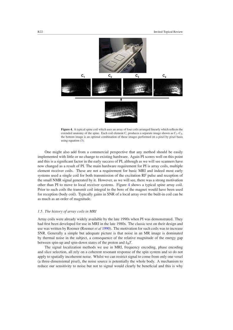
Figure 4. A typical spine coil which uses an array of four coils arranged linearly which reflects theextended anatomy of the spine. Each coil element C, produces a separate image shown as C1–C4,the bottom image is an optimal combination of these images performed on a pixel by pixel basisusing equation (3).
One might also add from a commercial perspective that any method should be easilyimplemented with little or no change to existing hardware. Again PI scores well on this pointand this is a significant factor in the early success of PI, although as we will see scanners havenow changed as a result of PI. The main hardware requirement for PI is array coils, multipleelement receiver coils. These are not a requirement for basic MRI and indeed most earlysystems used a single coil for both transmission of the excitation RF pulse and reception ofthe small NMR signal generated by it. However, as we will see, there was a strong motivationother than PI to move to local receiver systems. Figure 4 shows a typical spine array coil.Prior to such coils the transmit coil integral to the bore of the magnet would have been usedfor reception (body coil). Typically gains in SNR of a local array over the built-in coil can beas much as an order of magnitude.
1.5. The history of array coils in MRI
Array coils were already widely available by the late 1990s when PI was demonstrated. Theyhad first been developed for use in MRI in the late 1980s. The classic text on their design anduse was written by Roemer (Roemer et al 1990). The motivation for such coils was to increaseSNR. Generally a simple but adequate picture is that noise in an MR image is dominatedby thermal noise in the subject, a consequence of the relative magnitude of the energy gapbetween spin-up and spin-down states of the proton and kBT.
The signal localization methods we use in MRI, frequency encoding, phase encodingand slice selection, all rely on a coherent resonant response of the spin system and so do notapply to spatially incoherent noise. Whilst we can restrict signal to come from only one voxel(a three-dimensional pixel), the noise source is potentially the whole body. A mechanism toreduce our sensitivity to noise but not to signal would clearly be beneficial and this is why
Invited Topical Review R23
localized receiver coils are important. This can be illustrated by considering two simple loopantennas: a small one and a large one. For the purposes of this discussion, we shall assumefor the sake of simplicity that the signal sensitivity at a given voxel positioned above theircentrelines is the same for both coils. The contribution to the signal measured by a givencoil is stronger for spins located close to it, and becomes weaker the further they are fromthe coil. This property is designated by coil sensitivity and it is determined by the amountof magnetic flux generated at the voxel captured by the coil. In an imaging experiment thesignal is localized via the MRI process and so because the coils sensitivities are the same atthis location, both receive the same signal from this voxel. However the noise that each coilsees is proportional to the integrated sensitivity of the coil over the whole sample, which islarger for the larger coil. The SNR performance of this coil at this voxel is therefore less goodthan that of the small coil.
The benefit of the large coil becomes apparent if we consider a second voxel some distancefrom the first. In this case the sensitivity of the large coil exceeds that of the small coil and sothe SNR at this location is more favourable for the large coil. The development of the arraycoil stems naturally from this discussion. To have the SNR benefit of the small coil with thespatial coverage of a large coil independent multiple small elements are needed, i.e. an array.Array coils were developed to facilitate large field of view high SNR imaging. Each element ofan array coil must be attached to a separate independent receiver system to minimize couplingbetween elements, which would reduce the SNR benefit. So for a given imaging experimentmultiple full images, one for each coil element, can be reconstructed. We are then left withthe problem of how to combine these images for optimal SNR. Again Roemer explored thisproblem for us (Roemer et al 1990). Simple addition of the images produces a non-optimalreconstruction as the same voxel in each image has varying signal but the same level of noise.An optimal combination was shown by Roemer to be:
Sopt = wi
S1
C1+ wi
S2
C2+ wi
S3
C3+ · · · where wi = C2
i∑C2
j
. (3)
At a given voxel location the signal from each coil is weighted by the coil sensitivities (C)at this location. Here we used the convention that C2 = C∗ · C, where the asterisk denotescomplex conjugation. From this we can see that to optimally reconstruct array coil images weneed to explicitly know the coil sensitivities at all pixel locations. The sensitivity of a givencoil varies from voxel to voxel in three dimensions and its knowledge plays a crucial role in PI.However, when Roemer wrote this paper, the requirement that sensitivities had to be known(and therefore measured) was perceived to be onerous (probably because at that time gradientperformance was much lower than it is at present and so scan times were significantly longer,coil calibration would have taken minutes rather than the 30s or so it now takes) as it impliesacquiring a separate coil reference scan. For this reason Roemer went on to demonstrate thatfor almost all situations where SNR is intrinsically high a simple approximation of the sum ofsquares (SOS) provides a close to optimal reconstruction. This astute observation may wellhave been inadvertently responsible for slowing the rate of adoption of PI. Roemer’s paperwas written in 1990, shortly after the first parallel imaging proposals. The SOS approachwas widely (almost universally) adopted meaning that coil sensitivities were not routinelymeasured. If the SOS approximation had not been adopted, then all the tools for PI wouldhave been in place: the use of array coils and reference scans. As it was, calibration was notexplored until the emergence of PI in the late 1990s. Since then it has been demonstratedthat optimal reconstruction can be achieved even without explicit coil sensitivity maps byextracting this information from the images themselves (Bydder et al 2002a). Figure 4 showsa four-element spine array coil in its enclosure, the four individual images produced from
R24 Invited Topical Review
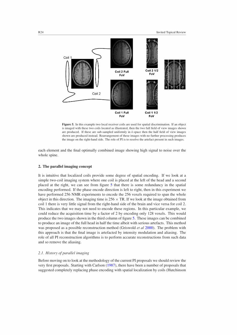
Figure 5. In this example two local receiver coils are used for spatial discrimination. If an objectis imaged with these two coils located as illustrated, then the two full field of view images shownare produced. If these are sub-sampled uniformly in k-space then the half field of view imagesshown are produced instead. Rearrangement of these images with no further processing producesthe image on the right-hand side. The role of PI is to resolve the artefact present in such images.
each element and the final optimally combined image showing high signal to noise over thewhole spine.
2. The parallel imaging concept
It is intuitive that localized coils provide some degree of spatial encoding. If we look at asimple two-coil imaging system where one coil is placed at the left of the head and a secondplaced at the right, we can see from figure 5 that there is some redundancy in the spatialencoding performed. If the phase encode direction is left to right, then in this experiment wehave performed 256 NMR experiments to encode the 256 voxels required to span the wholeobject in this direction. The imaging time is 256 × TR. If we look at the image obtained fromcoil 1 there is very little signal from the right-hand side of the brain and vice versa for coil 2.This indicates that we may not need to encode these regions. In this particular example, wecould reduce the acquisition time by a factor of 2 by encoding only 128 voxels. This wouldproduce the two images shown in the third column of figure 5. These images can be combinedto produce an image of the full head in half the time albeit with serious artefacts. This methodwas proposed as a possible reconstruction method (Griswold et al 2000). The problem withthis approach is that the final image is artefacted by intensity modulation and aliasing. Therole of all PI reconstruction algorithms is to perform accurate reconstructions from such dataand so remove the aliasing.
2.1. History of parallel imaging
Before moving on to look at the methodology of the current PI proposals we should review thevery first proposals. Starting with Carlson (1987), there have been a number of proposals thatsuggested completely replacing phase encoding with spatial localization by coils (Hutchinson
Invited Topical Review R25
and Raff 1988, Kwiat et al 1991). Such methods are sometimes referred to as ‘massivelyparallel’ methods. The ‘partial’ in PPI is used to clearly distinguish it from these earlymethods, which apply inverse source procedures to reconstruct an image of the object fromthe signals received by a large number, typically 128 coils. There are a number of problemswith such a proposal. Manufacturing large coil arrays holds major challenges and scannersat this time rarely had more than one receiver channel. It would be another almost twodecades before 128 channel machines even hit the drawing board. A much more significantimpediment to such non-phase encoded imaging is SNR. Whilst Fourier encoding via phaseencoding is time consuming, it has benefits as the SNR increases with the square root of thenumber of phase encodes. This is known as Fourier averaging and is essential to obtain theSNR we require for high quality imaging. If Fourier encoding is abandoned altogether, thenfor a 128 × 128 image matrix the SNR drops by an order of magnitude. (We will see that thisdependence of the SNR on the number of phase encoding steps becomes critical in assessingsuitable applications for PI.) In addition to this, the number of reconstructed pixels is fixed bythe number of coils. This severely limits the radiologists who need to be able to determine theresolution of the acquisition based on the anatomical detail they require, and not to be limitedby the coil number to these low resolutions. Such limitations have not deterred some recentresearchers lured by the incredible imaging speeds possible with single echo acquisition (SEA)from rising to the formidable engineering challenges inherent in trying to construct such asystem (McDougall and Wright 2005). Presently, these systems remain very much in theresearch arena with only very limited potential applications.
The first partially parallel imaging proposals, where coil encoding was used as anaugmentation to Fourier encoding, came in 1993 (Carlson and Minemura 1993). Neitherwere experimentally realized in vivo, with results limited to phantom objects. It was not untilSodickson’s seminal abstract at the 1997 meeting of the International Society of MagneticResonance in Medicine (ISMRM), and his follow-up paper (Sodickson et al 1999), that thecommunity really embraced the potential of these methods. The reason was simple. Notonly did Sodickson propose a method but he implemented it in one of the most challengingapplications of all: cardiac imaging. Cardiac imaging had until this point been limitedseverely by gradient performance and the desire for whole heart free breathing imagingwas not realizable without breaking this limit. Sodickson’s paper was received with greatexcitement amongst the few that realized its implications. One such group, Pruessmannet al, realized, with hindsight, that the rather clumsy formulation proposed by Sodicksoncould be made much simpler if the problem were stated in the image domain rather thanin k-space, as Sodickson had proposed. This leads to the sensitivity encoding (SENSE)method which was presented the following year at ISMRM and eventually published in 1999(Pruessmann et al 1999). Following these two pioneers, a slew of reconstruction methodswere proposed. It is beyond the scope of this review to give a detailed review of all of these asthere are great similarities and overlap. However, the next section will explore four methodswhich represent a good cross-section of the types of methods available. Allied methods willbe referenced in each section.
2.2. Reconstruction algorithms
Firstly we look at an image domain method (SENSE) where both the coil reference dataand the sub-sampled target data are operated on in the image domain. The second method(SMASH) keeps the coil information in the image domain but operates on the target data ink-space. The third approach (generalized-SMASH) keeps both reference and target data ink-space. In the final method presented (GRAPPA) all data are again in k-space but there are
R26 Invited Topical Review
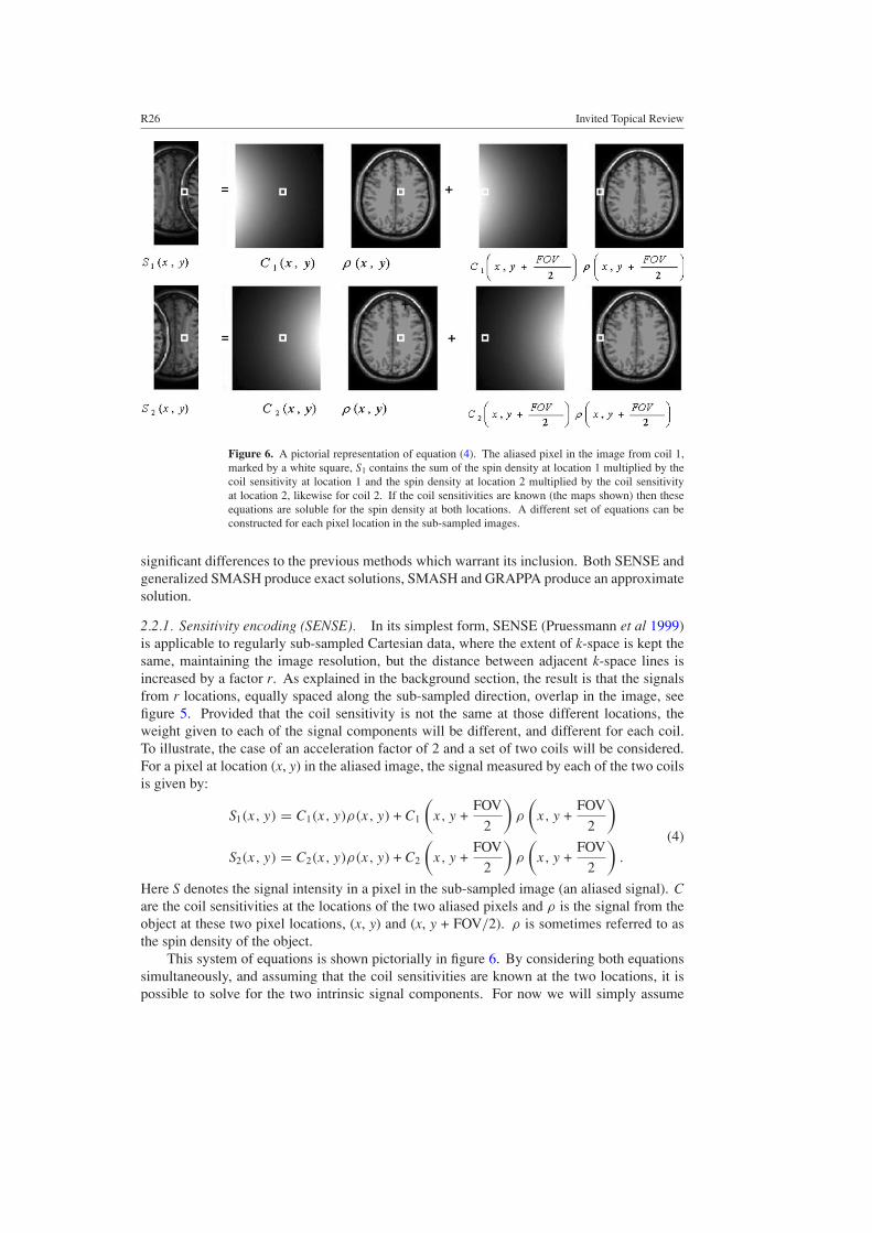
Figure 6. A pictorial representation of equation (4). The aliased pixel in the image from coil 1,marked by a white square, S1 contains the sum of the spin density at location 1 multiplied by thecoil sensitivity at location 1 and the spin density at location 2 multiplied by the coil sensitivityat location 2, likewise for coil 2. If the coil sensitivities are known (the maps shown) then theseequations are soluble for the spin density at both locations. A different set of equations can beconstructed for each pixel location in the sub-sampled images.
significant differences to the previous methods which warrant its inclusion. Both SENSE andgeneralized SMASH produce exact solutions, SMASH and GRAPPA produce an approximatesolution.
2.2.1. Sensitivity encoding (SENSE). In its simplest form, SENSE (Pruessmann et al 1999)is applicable to regularly sub-sampled Cartesian data, where the extent of k-space is kept thesame, maintaining the image resolution, but the distance between adjacent k-space lines isincreased by a factor r. As explained in the background section, the result is that the signalsfrom r locations, equally spaced along the sub-sampled direction, overlap in the image, seefigure 5. Provided that the coil sensitivity is not the same at those different locations, theweight given to each of the signal components will be different, and different for each coil.To illustrate, the case of an acceleration factor of 2 and a set of two coils will be considered.For a pixel at location (x, y) in the aliased image, the signal measured by each of the two coilsis given by:
S1(x, y) = C1(x, y)ρ(x, y) + C1
(x, y +
FOV
2
)ρ
(x, y +
FOV
2
)(4)
S2(x, y) = C2(x, y)ρ(x, y) + C2
(x, y +
FOV
2
)ρ
(x, y +
FOV
2
).
Here S denotes the signal intensity in a pixel in the sub-sampled image (an aliased signal). Care the coil sensitivities at the locations of the two aliased pixels and ρ is the signal from theobject at these two pixel locations, (x, y) and (x, y + FOV/2). ρ is sometimes referred to asthe spin density of the object.
This system of equations is shown pictorially in figure 6. By considering both equationssimultaneously, and assuming that the coil sensitivities are known at the two locations, it ispossible to solve for the two intrinsic signal components. For now we will simply assume
Invited Topical Review R27
that the coil sensitivities are known. Later on we will describe how coil sensitivities can bemeasured experimentally through a reference scan.
The equation above can be written in matrix form as:
S = Cρ (5)
where C is a matrix with N rows, corresponding to the number of coils, and r columns for thenumber of overlapping pixels. The problem can be generalized to any number of coils andacceleration factor. In order for this set of equations to be solvable, it is therefore necessaryto collect data with at least as many different coils as the acceleration factor r. The intrinsicsignal may be obtained through a least-squares approach, by calculating the general inverseof the coil sensitivity matrix. To take into account possible differences in noise levels and thenoise correlation between different coil channels, the receiver noise matrix � is included inthe reconstruction:
ρ′ = (CHΨ−1C)−1CHΨ−1S. (6)
Here ρ′ indicates the reconstructed estimate of ρ. The matrix Ψ can be estimated throughthe analysis of data acquired in the absence of MR signal. Letting ηi denote the noise sampleacquired by coil i, the Ψij entry of the noise matrix is given by:
Ψij = ηiη∗j (7)
with the bar indicating time averaging.Reducing the number of phase encode lines leads in itself to a reduction in SNR of
√r
due to reduced Fourier averaging. Also the SNR at each pixel in the reconstructed image willdepend on how easily this matrix inversion can be performed, i.e. on how different the coilsensitivities are at the aliased pixels. There is therefore an extra term which needs to be takeninto account when comparing the SNR measured with reduced phase encoding, compared towhen full encoding is done: the so-called geometry factor or g-factor, which is dependent onthe particular geometry of the coil array. For a pixel p the relationship can be written in thefollowing way:
SNRredp = SNRfull
p
gp
√r
. (8)
The g-factor has become a standard method of assessing any parallel imaging algorithm.When applying the SENSE algorithm, the g-factor at pixel p can be directly calculatedfrom
gp =√
[(CH�−1C)−1]p,p[(CH�−1C)]p,p. (9)
We will discuss the g-factor further in the limits section.When regular sub-sampling is used, only pixels located along the phase encode direction
and at well-determined distances from each other (related to the distance between sampledpoints in k-space) will overlap in the undersampled image. This allows breaking down thegeneral problem into a series of small equations solved separately for each aliased pixel groupas explicitly described in (4). The solution comes from the inversion of small matrices. Fora reduction factor of r, it would be necessary to invert N/r r × r-sized matrices. This pixelgroup by pixel group approach is the simplest PI reconstruction method and is sometimesreferred to as ‘simple SENSE’.
If sub-sampling along the phase encode direction is no longer regular, as in the exampleseen in figure 2(d), every pixel within a row of the image may potentially alias with eachother. In this case the problem is only separable for pixels located at different positions along
R28 Invited Topical Review
the read direction and so larger matrices are required to be inverted, increasing computationalcomplexity and therefore reconstruction time.
In the general case of variable sub-sampling in all directions in k-space, every pixel canpotentially alias with all the others and there is no alternative but to try and invert the wholeencoding matrix. Given the very large size of this matrix (N2 × N2 for a square image sizedN × N), the memory requirements and the time needed to solve this problem would be toolarge to be practical. Fortunately there are numerical methods which enable us to solvethe problem in an iterative way, without having to explicitly calculate the inverse matrix.The conjugate gradient (CG) approach, for instance, can be used to solve linear systems of theform Ax = b, provided that the matrix A is positive definite (Hestenes 1952). Although this isnot generally the case, the original set of equations (5) can be altered so that the matrix to beinverted (CHΨ−1C) obeys this requirement (Pruessmann et al 2001b):
(CHΨ−1C)ρ = CHΨ−1S. (10)
A further simplification is possible, whereby modifying both the encoding matrix and thesampled data, the noise matrix can be removed from the equation above (Pruessmann et al2001b).
In practice this inversion problem can be solved more efficiently by replacing some ofthe steps implicit in the encoding matrix with their equivalent functional forms. Fouriertransforms, for example, can be applied using the fast Fourier transform algorithm (FFT),instead of having to build a matrix containing the required Fourier terms. This approach canalso be applied to non-Cartesian schemes provided that forward and reverse gridding steps areintroduced (Pruessmann et al 2001b).
2.2.2. Simultaneous acquisition of spatial harmonics (SMASH). Although it was theintroduction of SENSE that really pushed the field of parallel imaging forward, the useof multiple receivers coils to speedup acquisition had already been demonstrated in vivoby Sodickson and Manning (1997). The reconstruction technique they developed is calledSMASH. In this case the reconstruction is performed with the target data in the k-space domain,while the coil sensitivities are kept in image space. In order to understand how k-space-basedmethods work, it is important to bear in mind the signal equation, relating the k-space signalsampled by a coil j with sensitivity Cj(x, y) to the spin density of the object being imagedρ(x, y):
Sj (kx, ky) =∫ ∫
Cj(x, y)ρ(x, y) exp(−ikxx) exp(−ikyy) dx dy. (11)
Here the Fourier relationship between image domain and k-space is written explicitly as theintegral over x and y.
In SMASH the coil sensitivities are used to explicitly perform the omitted phase encodingsteps. Figure 3 shows that a field of view reduction increases the spacing between samples ink-space. Each phase encoding gradient applied imparts a sinusoidal phase modulation acrossthe whole object. It is this modulation that ‘shifts’ the measured data in k-space. In SMASHthe coil sensitivities are fitted to idealized phase encode shift functions which are then appliedto repopulate missing lines in k-space. The coil sensitivities are linearly combined so as toapproximate the required spatial harmonics. For a speedup factor of r, this means that allspatial harmonics from the 0th (a constant) till the rth order need to be synthesized. Theweight given to each coil to generate each of these harmonics can be determined through aleast-squares fit. For the mth spatial harmonic this is equivalent to determining the weights
Invited Topical Review R29
wmj in the equation below, where j is the coil index counting from 1 to the number of coils N,
Cj represent the coil sensitivity for the jth coil and �ky = 2πFOVy
.∑
j
wmj Cj (x, y) = exp(−im�kyy). (12)
An example of how spatial harmonics can be generated by combining coil sensitivities isshown in figure 7.
These weights can then be used to combine the signals measured for each coil and generatea composite signal at both sampled and originally un-sampled locations. This is equivalent tocombining together (11) and (12):∑
j
wmj Sj (kx, ky) ≈
∫ ∫ρ(x, y) exp(−ikxx) exp(−ikyy) exp(−im�kyy) dx dy
= S(kx, ky + m�ky). (13)
The problem with this approach is that it is not valid for general coil geometries. In order forSMASH to work, it must be possible to construct good approximations to the spatial harmonicsrequired. While this may be reasonable for a linear coil array provided that the coil structureis adequately related to the image FOV, it is difficult to achieve good results in many cases.
2.2.3. Generalized-SMASH (g-SMASH). Although the introduction of both SMASH andsimple SENSE represented a major breakthrough, it was clear that new algorithms needed tobe developed in order to try and overcome their limitations. Two important goals were to enablethe use of general coil geometries, as in SENSE, and also to be able to sub-sample k-spacealong the phase encode direction in a non-regular way if so desired. The second requirementwas not applicable to SENSE in its initial implementation but, as already explained, a moregeneral approach was later developed which allows for the use of arbitrary k-space samplingschemes (Pruessmann et al 2001b).
Two schemes developed to overcome these problems were g-SMASH (Bydder et al 2002c)and ‘Sensitivity profiles from an array of coils for encoding and reconstruction in parallel’SPACE-RIP (Kyriakos et al 2000). In the case of g-SMASH, the reconstruction is performedwith the coil data in k-space. This is the main difference between this method and SPACE-RIP,in which case the coil data are kept in the image domain. Due to their similarity, only the firstmethod will be examined here and the modifications required to implement the second onediscussed.
g-SMASH is based on a similar expression to (12) for SMASH. In this case, however, theequation is reversed and the sensitivity of each coil expressed as a sum of Fourier terms alongthe phase encode direction:
Cj(x, y) =q∑
m=−p
amj exp(−im�kyy). (14)
Given that the data are fully sampled along the read direction, it is possible to take the Fouriertransform of the signal equation (11) along the read direction, taking the data into hybridspace:
Sj (x, ky) =∫
Cj(x, y)ρ(x, y) exp(−ikyy) dy. (15)
By replacing the coil sensitivities in the above equation with the expression in (14) it is possibleto relate the coil modulated signal, which is measured, with the intrinsic MR signal which is

R30 Invited Topical Review
Figure 7. If we take the example of the four coil elements from the spine coil in figure 4 thenthe sensitivity profiles plotted along the long axis are seen on the left-hand side of the figure. Theindividual profiles can be seen as a thin line and the summed profiles as the solid line. In thesimplest form of SMASH this sum is assumed to be constant over the field of view and as suchrepresents the weights required for the zeroth term in k-space. An example of a higher order termis seen on the right. Here the coil combination weights have been set as shown and a sinusoidalmodulation has been constructed across the image. This combination produces a shift in k-spaceallowing missing lines to be filled in.
unknown:
Sj (x, ky) =q∑
m=−p
amj
∫ρ(x, y) exp(−ikyy) exp(−im�kyy) dy =
q∑m=−p
amj S(x, ky + m�ky).
(16)
Given that for samples taken at neighbouring points there is an overlap between the involvedS(x, ky − p�ky) to S(x, ky + q�ky) terms, all the equations corresponding to the same valueof x can be combined. The different versions of (16) for each coil can also be consideredsimultaneously. Solving these sets of linear equations will thus be equivalent to inverting alarge encoding matrix E, where the N matrices corresponding to each of the individual coilsare vertically stacked.
S1(x)
· · ·SN(x)
=
E1(x)
· · ·EN(x)
S(x). (17)
Given that the product of Ej(x) and S(x) represents a convolution, each matrix Ej(x) is formed bycyclic permutations of a vector containing the Fourier terms aj
m(x). This gives the encodingmatrices a very particular appearance as shown in figure 8 for the simpler case of regularsub-sampling.
To obtain the equivalent expression for SPACE-RIP, it is only necessary to insert a Fouriertransform F and its inverse between the Ej and S matrices:
Sj = Ej (F−1F)S = (Ej F−1)(FS). (18)
By doing so the coil matrix (Ej F−1) and the reconstructed data (FS) will no longer be in the(x, ky) hybrid space, but in the image domain. It is important to note, however, that becausecoil data can be represented more compactly in k-space, the encoding matrix is sparser in thisrepresentation which means that its inversion is more efficient in the case of g-SMASH.
The main benefit of either of these methods is that they are compatible with the use ofnon-regular sampling schemes. This is advantageous in cases where it is possible to extract thecoil sensitivities from the data itself, without the need to perform separate reference scans and
Invited Topical Review R31
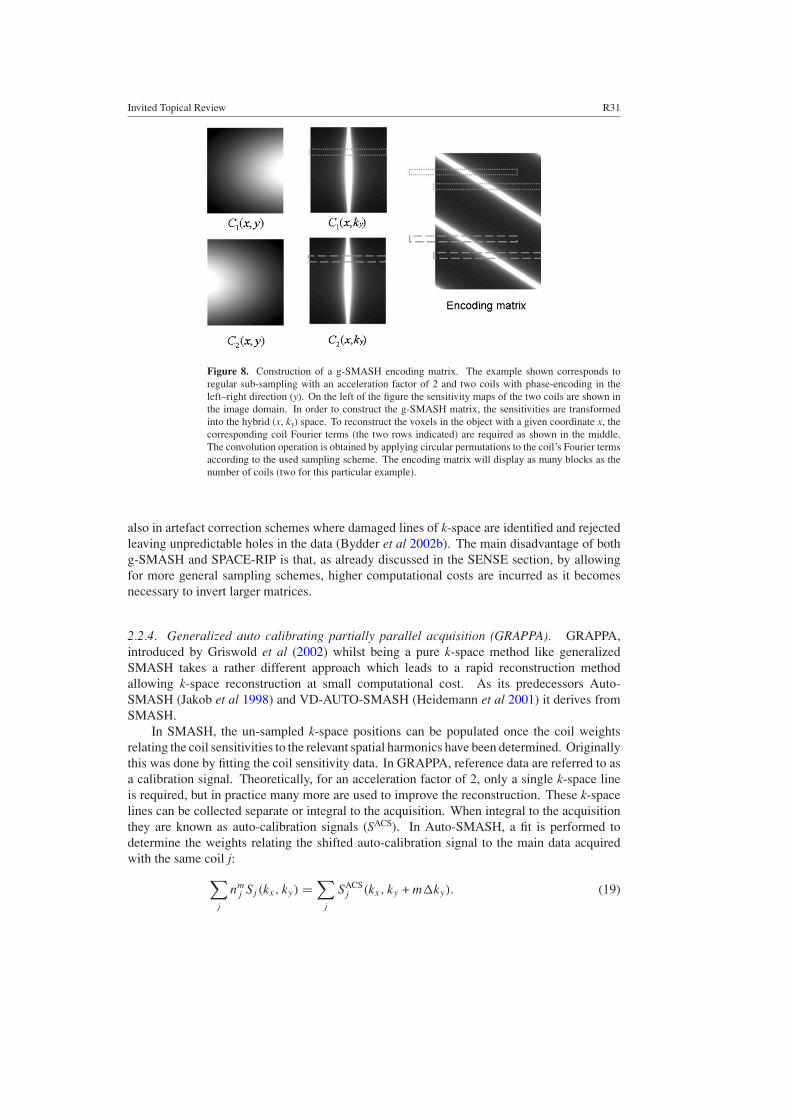
Figure 8. Construction of a g-SMASH encoding matrix. The example shown corresponds toregular sub-sampling with an acceleration factor of 2 and two coils with phase-encoding in theleft–right direction (y). On the left of the figure the sensitivity maps of the two coils are shown inthe image domain. In order to construct the g-SMASH matrix, the sensitivities are transformedinto the hybrid (x, ky) space. To reconstruct the voxels in the object with a given coordinate x, thecorresponding coil Fourier terms (the two rows indicated) are required as shown in the middle.The convolution operation is obtained by applying circular permutations to the coil’s Fourier termsaccording to the used sampling scheme. The encoding matrix will display as many blocks as thenumber of coils (two for this particular example).
also in artefact correction schemes where damaged lines of k-space are identified and rejectedleaving unpredictable holes in the data (Bydder et al 2002b). The main disadvantage of bothg-SMASH and SPACE-RIP is that, as already discussed in the SENSE section, by allowingfor more general sampling schemes, higher computational costs are incurred as it becomesnecessary to invert larger matrices.
2.2.4. Generalized auto calibrating partially parallel acquisition (GRAPPA). GRAPPA,introduced by Griswold et al (2002) whilst being a pure k-space method like generalizedSMASH takes a rather different approach which leads to a rapid reconstruction methodallowing k-space reconstruction at small computational cost. As its predecessors Auto-SMASH (Jakob et al 1998) and VD-AUTO-SMASH (Heidemann et al 2001) it derives fromSMASH.
In SMASH, the un-sampled k-space positions can be populated once the coil weightsrelating the coil sensitivities to the relevant spatial harmonics have been determined. Originallythis was done by fitting the coil sensitivity data. In GRAPPA, reference data are referred to asa calibration signal. Theoretically, for an acceleration factor of 2, only a single k-space lineis required, but in practice many more are used to improve the reconstruction. These k-spacelines can be collected separate or integral to the acquisition. When integral to the acquisitionthey are known as auto-calibration signals (SACS). In Auto-SMASH, a fit is performed todetermine the weights relating the shifted auto-calibration signal to the main data acquiredwith the same coil j:
∑j
nmj Sj (kx, ky) =
∑j
SACSj (kx, ky + m�ky). (19)

R32 Invited Topical Review
Figure 9. A 5 × 4 GRAPPA reconstruction kernel is illustrated for an acceleration factor of 2with three coils. The points in grey correspond to the normally acquired sub-sampled data, whileauto-calibration signal (ACS) lines are shown in black. The un-acquired points are not shown. Inorder to estimate the signal at these points, the weights that relate the signal at a particular locationwith that of its neighbours must first be determined. The fitting process is performed to the extraACS lines. Depending on the choice of kernel, the group of pixels considered in the fitting willvary. For these particular dimensions (5 × 4), and to fit, for example, the ACS signal acquired bycoil 2 at location (kx, ky) as indicated by the white circle, all points within the three black boxesshown would be used.
These weights are subsequently applied to construct the un-sampled lines. The differencebetween Auto-SMASH and VD-AUTO-SMASH is that in the latter case more than theminimum amount of k-space lines (r − 1, where r is the acceleration factor) are acquiredin order to determine the coil weights more accurately.
A feature of GRAPPA reconstructions is that separate images are reconstructed for eachcoil. These can be combined finally by any means desired (typically SOS). In order todetermine the reconstruction weights the following expression is employed:
Sj (kx, ky + m�ky) =∑
l
∑b
n(j, b, l,m)Sl(kx, ky + br�ky) (20)
where r is the acceleration factor and b is an index that counts through the multiple lines usedin the reconstruction. The implementation of GRAPPA was later improved, and the size ofthe kernel used for determining the coil weights extended so as to consider also points alongthe kx direction (Wang et al 2005). For a 5 × 4 kernel the reconstruction could be written as
Sj (kx, ky + m�ky) =N∑
l=1
2∑a=−2
1∑b=−2
n(j, a, b, l,m)Sl(kx + a�kx, ky + (br + 1)�ky). (21)
A kernel of this size is illustrated in figure 9.The size of the kernel used in the reconstruction is chosen by the user. If all acquired
data points were used, a more exact reconstruction would be obtained. However, as the moresignificant weights are the ones relating neighbouring points, smaller blocks can be considered
Invited Topical Review R33
without significant penalties in terms of image fidelity. This truncation is advantageous in thatit reduces the computational times required. The reason why it is possible to use small kernelsis that normally the coil sensitivities can be described by a small number of Fourier terms. Theextent of information in k-space is therefore contained within the immediate neighbourhoodof each k-space data point considered.
2.3. Discussion
It is important to note that if accurate coil sensitivity maps are available, it is preferable to usefull reconstruction methods such as SENSE (simple or generalized) or generalized SMASH asthe other methods discussed here, SMASH and GRAPPA, are approximate solutions resultingfrom a least-squares optimized fit to spatial harmonics. However, there are cases whenobtaining precise coil sensitivity data may be difficult and in these cases the fitting procedurecan constrain the solutions to produce more benign errors in the final reconstruction.
A major difference between these methods is computation time. Simple SENSE, SMASHand GRAPPA are rapid enough to be used ‘real time’ on scanners. The other methods allhave too high a computational cost to be available in real time. SMASH in its original form issusceptible to severe artefacts but modified versions e.g. VD-AUTO-SMASH are more robust.
3. Implementation
In MRI the raw data that we acquire are complex (have a magnitude and a phase component).Generally we ignore the phase component when viewing images and in the examples shownin figures in this review only the magnitude components of both target and coil reference datahave been shown for simplicity. However, phase plays a crucial role in the reconstructionprocess in PI. The coil sensitivity varies in space in both phase and magnitude and so keepingthe phase information is required to make accurate reconstructions. All the linear algebradescribed in the algorithms section is performed on complex data sets. The final reconstructedimage can then be displayed conventionally as magnitude only images. For this reason even theimage domain reconstruction processes have to intercept raw data on the scanner rather thanbe applied post the usual image production process. Coil reference data, if acquired separatelyalso have to be stored in its complex form to be used in subsequent image reconstructions.
3.1. Coil calibration
The majority of algorithms for image reconstruction are robust and have well-definedproperties. However, the final image is in general only as good as the data that are input intoit (we will look at some cases where PI can improve the quality of the image reconstruction inthe final section). In PI there are two types of data used, the image data and the coil referencedata. In a practical implementation of PI the acquisition and subsequent treatment of the coilreference data is of crucial importance. The impact of the reference data on the final imageshould be completely benign, which requires the coil reference data to be ideally noiselessand perfectly accurate. Such requirements are almost achievable in practice if care is taken inthe measurement.
For all the image reconstruction methods described in this review, low resolution referencedata is required but the domain in which it is used varies (a slight variant on this is GRAPPAwhich does not explicitly extract coil information from object information, we will return tothis later in this section). Subject dependent calibration is required for reasons discussed laterin section 3.4.2.
R34 Invited Topical Review
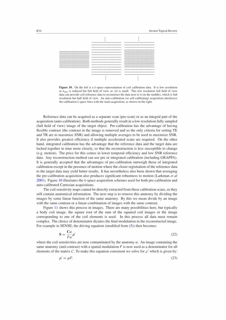
Figure 10. On the left is a k-space representation of coil calibration data. It is low resolutionas kmax is reduced but full field of view, as �k is small. This low resolution full field of viewdata can provide coil reference data to reconstruct the data next to it (in the middle), which is fullresolution but half field of view. An auto-calibration (or self-calibrating) acquisition interleavesthe calibration k-space lines with the main acquisition, as shown on the right.
Reference data can be acquired as a separate scan (pre-scan) or as an integral part of theacquisition (auto-calibration). Both methods generally result in a low resolution fully sampled(full field of view) image of the target object. Pre-calibration has the advantage of havingflexible contrast (the contrast in the image is removed and so the only criteria for setting TEand TR are to maximize SNR) and allowing multiple averages to be used to maximize SNR.It also provides greatest efficiency if multiple accelerated scans are required. On the otherhand, integrated calibration has the advantage that the reference data and the target data arelocked together in time more closely, so that the reconstruction is less susceptible to change(e.g. motion). The price for this comes in lower temporal efficiency and low SNR referencedata. Any reconstruction method can use pre or integrated calibration (including GRAPPA).It is generally accepted that the advantages of pre-calibration outweigh those of integratedcalibration except in the presence of motion where the closer registration of the reference datato the target data may yield better results. It has nevertheless also been shown that averagingthe pre-calibration acquisition also produces significant robustness to motion (Larkman et al2001). Figure 10 illustrates the k-space acquisition schemes used for both pre-calibration andauto-calibrated Cartesian acquisitions.
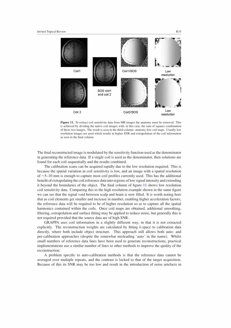
The coil sensitivity maps cannot be directly extracted from these calibration scans, as theystill contain anatomical information. The next step is to remove this anatomy by dividing theimages by some linear function of the same anatomy. By this we mean divide by an imagewith the same contrast or a linear combination of images with the same contrast.
Figure 11 shows this process in images. There are many possibilities here, but typicallya body coil image, the square root of the sum of the squared coil images or the imagecorresponding to one of the coil elements is used. In this process all data must remaincomplex. The choice of denominator dictates the final modulation in the reconstructed image.For example in SENSE, the driving equation (modified from (5)) then becomes
S = Cα
Fαρ′ (22)
where the coil sensitivities are now contaminated by the anatomy α. An image containing thesame anatomy (and contrast) with a spatial modulation F is now used as a denominator for allelements of the matrix C. To make this equation consistent we solve for ρ ′ which is given by:
ρ′ = ρF. (23)
Invited Topical Review R35
Figure 11. To extract coil sensitivity data from MR images the anatomy must be removed. Thisis achieved by dividing the native coil images with, in this case, the sum of squares combinationof these two images. The result is seen in the third column: anatomy free coil maps. Usually lowresolution images are used which results in higher SNR and extrapolation of the coil informationas seen in the final column.
The final reconstructed image is modulated by the sensitivity function used as the denominatorin generating the reference data. If a single coil is used as the denominator, then solutions arefound for each coil sequentially and the results combined.
The calibration scans can be acquired rapidly due to the low resolution required. This isbecause the spatial variation in coil sensitivity is low, and an image with a spatial resolutionof ∼5–10 mm is enough to capture most coil profiles currently used. This has the additionalbenefit of extrapolating the coil reference data into regions of low signal intensity and extendingit beyond the boundaries of the object. The final column of figure 11 shows low resolutioncoil sensitivity data. Comparing this to the high resolution example shown in the same figurewe can see that the signal void between scalp and brain is now filled. It is worth noting herethat as coil elements get smaller and increase in number, enabling higher acceleration factors,the reference data will be required to be of higher resolution so as to capture all the spatialharmonics contained within the coils. Once coil maps are obtained, additional smoothing,filtering, extrapolation and surface fitting may be applied to reduce noise, but generally this isnot required provided that the source data are of high SNR.
GRAPPA uses coil information in a slightly different way, in that it is not extractedexplicitly. The reconstruction weights are calculated by fitting k-space to calibration datadirectly, where both include object structure. This approach still allows both auto- andpre-calibration approaches (despite the somewhat misleading ‘auto’ in the name). Whilstsmall numbers of reference data lines have been used to generate reconstructions, practicalimplementations use a similar number of lines to other methods to improve the quality of thereconstruction.
A problem specific to auto-calibration methods is that the reference data cannot beaveraged over multiple repeats, and the contrast is locked to that of the target acquisition.Because of this its SNR may be too low and result in the introduction of noise artefacts in
R36 Invited Topical Review
the reconstructed image. For auto-calibration methods where the coil information is extracteddirectly, smoothing and fitting of the coil data is recommended to reduce sensitivity to noise.
A final stage in the production of coil data is to threshold out the background. Thisexcludes pixels which do not contain the object from processing. This reduces ill conditioningof the reconstruction by including the prior knowledge that the correct signal value for theselocations is zero. However, when performing this step it is important to ensure that the mask isnot too harsh as otherwise regions at the edge of the object may also be erroneously excluded(Haselgrove and Prammer 1986). Artefacts can appear in the reconstructed images if veryaggressive masks are used. This type of problem can be avoided by lowering the thresholdwhile increasing the level of smoothing. Additional extrapolation of the original mask can alsobe performed (Pruessmann et al 1999). The optimal choice of threshold, smoothing levelsand size of the extrapolated regions results in a compromise. On one hand the amount ofnoise in the reference data should be reduced as much as possible but on the other hand, onehas to ensure that no object regions are excluded from the sensitivity data due to excessivethresholding.
3.2. Intrinsic limits
PI acceleration is achieved at a cost in SNR. As shown in (8) the loss in SNR is due to twofactors: firstly, a reduction proportional to the square root of the speedup factor which occursdue to reduced temporal averaging. The remaining term, the g-factor, measures the level ofnoise amplification which occurs as a result of the reconstruction process. This value dependson how different the coil sensitivities are at the aliased pixels, so as to be able to distinguishthe signal contribution from each location, and is therefore dependent on the number andconfiguration of the coils. In general we use many more coils than the acceleration factor.This provides us with a vastly overdetermined system of equations and improves the numericalcondition of the matrix inversion at the heart of the algorithms discussed.
In practice, by using carefully designed coil arrays with six to eight elements, it has beenpossible to attain a speedup factor of 3 along one dimension with acceptable (this being asomewhat arbitrary definition) g-factor penalties (mean g-factors of 1.4 or 1.6 and maximumof up to 2.9) (Weiger et al 2001, de Zwart et al 2002). Unfortunately, the g-factor seems toincrease very abruptly if higher acceleration rates are attempted (Weiger et al 2001) and sothe g-factor is thought to represent an intrinsic limit to PI.
This assumption has led to the investigation of the intrinsic limits of PI. The question iswhether there is a fundamental limit to the achievable speedup factor, even when assumingthat an optimal coil array could be used. Ohliger et al (2003) and Wiesinger et al (2004a) haveanalysed the problem looking at the electrodynamics of the detection process. They noted thatthe signal and noise are necessarily coupled as they are associated with magnetic and electricfields respectively, which are linked through the Maxwell equations. Further constraints areimposed by the characteristics of the tissues, such as their conductivity and dielectric constants,which in turn depend, through the resonance frequency, on the strength of the static magneticfield. These studies concluded that provided that low or moderate reduction factors are used,the minimum g-factor achievable does remain close to the ideal value of 1. However, forreduction factors above a certain critical limit, the minimum g-factor increases exponentiallyleading to prohibitively low SNR levels.
For field strengths up to 5 T, it was found that the maximum reduction factor, correspondingto an arbitrary g-factor value of 1.2, is between 3 and 4 for undersampling along one dimension(Wiesinger et al 2004a). These simulations were performed considering an idealized sphericalobject with physical properties and dimensions close to those of a human head. However it

Invited Topical Review R37
was shown that higher total acceleration factors can be attained by distributing the aliasingalong multiple dimensions (Wiesinger et al 2004a, Ohliger et al 2003).
A further conclusion from these two theoretical studies, was that parallel imaging shouldbenefit from increased field strengths (Wiesinger et al 2004a, Ohliger et al 2003). As fieldmagnitude increases, the RF wavelength is reduced so that eventually a transition occursbetween the near-field (large wavelength) and far-field regimes (small wavelength). Giventhat the coil sensitivities become more structured in the far-field regime due to propagationand interference effects within the imaged object (Wiesinger et al 2006), the sensitivities ofthe individual elements of an array become more dissimilar to each other as the field strengthincreases. This results in an improved capacity to perform spatial encoding. The maximumacceleration factor therefore increases with field strength once the critical field value hasbeen exceeded. The transition between the two types of regime occurs for a field strengthcorresponding to a wavelength comparable to the size of the object. For a sphere of 20 cmof diameter, taken as an approximation to the shape of the human head, the critical field isbetween 4 and 5 T (Wiesinger et al 2006).
The benefits of increasing field strength were later confirmed experimentally, using theprinciple of electrodynamic scaling (Wiesinger et al 2004b). This method mimics the effectsof increasing field strength without actually having to deal with the difficulties involved inaccessing systems across the required field strength range. This was achieved by modifying thedielectric constant and conductivity of a phantom. The first is set by varying the proportionsof two miscible liquids with very different dielectric constants, whereas the conductivity canbe adjusted through the addition of different quantities of a soluble electrolyte.
Further support to the theoretical prediction that higher reduction factors can be attainedat higher fields has since been provided with the development of 7 T human systems. Initialin vivo measurements at this field strength have resulted in g-factor values much lower thanthose observed in comparable conditions at low field, with mean g-values of 1.26 for a reductionfactor of 4 (Adriany et al 2005).
Although it is now well established that increased field strengths should enable higherreduction factors, the g-factor values observed experimentally are still higher than the predictedminima. This means that there is still some margin for improvement in coil design for PIapplications. Unfortunately, by using improved set of coils one can only hope to reduce theeffective g-factor to values closer to, but not lower than, the intrinsic limits.
In response to these observed limits, some alternative strategies using prior informationor numerical tools have been developed to control the level of noise and artefact amplificationin the reconstructed image.
Reconstructing the image ρ′ from the measured data S requires the inversion of anencoding matrix C as implied in (5). One way to understand how noise amplification occursin parallel imaging reconstruction is to consider the singular value decomposition (SVD) ofthe m × n encoding matrix C:
C = UVH (24)
where Σ is an m × n matrix containing the nonnegative singular values σ i in the diagonal andzeros off the diagonal, and U and V are two square unitary matrices with dimensions m × mand n × n.
When all the singular values have the same value, small changes in the measured data donot have a significant impact on the reconstructed image. The encoding matrix is then said tobe well-conditioned and the condition number, the ratio between the largest and the smallesteigenvalues, is in this case equal to the ideal value of 1.
R38 Invited Topical Review
However if, for example, one of the singular values is much smaller than all the others,the corresponding singular value of the inverse matrix will be much larger than all the rest.Under these conditions, even a small amount of noise in the data, provided that it has somecomponent along the direction of the eigenvector associated with this particular eigenvalue,will result in large differences in the reconstructed image. In this case a high condition numberwill be associated with the encoding matrix.
One possible strategy to limit noise amplification is to set all the eigenvalues which arelower than a certain threshold to zero (σ i = 0 for all i > k). In these circumstances, thecorresponding eigenvalues associated with the inverse matrix will now be null and the level ofnoise in the reconstructed image is significantly reduced. The solution computed in this wayis called the truncated SVD solution and constitutes an approximation to the full solution. Bydiscarding the smallest singular values the noise in the image can be controlled at the cost oflosing some information regarding the object. Normally the threshold ε is chosen in a positionin the sequence of singular values where a large gap occurs: σ k > ε � σ k+1. This typeof strategy can be applied with reconstruction algorithms such as g-SMASH or SPACE-RIPfor which the matrices to be inverted (one per image column) are sufficiently large so thatthe fraction of singular values retained still provides a reasonable approximation to the truesolution.
However, in the case of standard SENSE a set of small matrices, each associated witha different group of aliased pixels, needs to be inverted instead. As the number of singularvalues for each of these matrices is already very small, truncated SVD is not an adequateapproach. Traditionally the method most used here is to add an extra term to the minimumleast-squares formulation (King and Angelos 2001). When using the least-squares approachto solve a set of linear equations, the goal is to minimize the error between the measured andthe predicted signal:
minρ′
‖Cρ′ − S‖2. (25)
To prevent large noise amplification, an extra term is added that penalizes solutions for ρ
having very large norms:
minρ′
‖Cρ′ − S‖2 + α2‖ρ′‖2. (26)
This method is known as damped least-squares or Tikhonov regularization. The factor α2 inthe equation above is known as Tikhonov factor (Tikhonov and Arsenin 1977). By adjustingthe value of this factor, more importance can be given to either of the two terms, with highTikhonov factors leading to reduced noise at a cost of increased aliasing artefacts in thereconstructed image and vice versa (King and Angelos 2001). Using methods such as theL-curve algorithm, an optimum regularization factor can be determined corresponding to agood trade-off between the two effects (Hansen 1998). The second term in (26) can be furthermodified so as to include prior information regarding the solution (Lin et al 2004).
An alternative approach to these regularization methods is to include prior knowledge ofthe object into the reconstruction (Larkman et al 2006). These methods are currently confinedto research applications. An example of such a method uses image domain joint entropybetween the data being reconstructed and a second image of the object. This method canbe understood by looking at how noise in the measured data affects the reconstruction. Bychoosing ρ and S to represent the image and measured signal in the ideal situation where nonoise is present, it is possible to see that the errors in the reconstruction (δρ) come from theaction of the inverse of the encoding matrix on the noise δS:
ρ + δρ = C−1(S + δS) (27)
Invited Topical Review R39
so that
δρ = C−1δS. (28)
This method estimates the error δρ by treating the noise δS as a free optimization parameter.The reconstructed image (ρ + δρ) can then be corrected and an image closer to the idealrecovered. However, in order for this to be achievable, it is necessary to reduce the searchspace by constraining the problem. The assumption is that as a system becomes less well-conditioned, the relative weight of the largest eigenvalue of the inverse of the encoding matrixbecomes larger. The principal singular value can come to represent a significant fraction ofthe average of all eigenvalues. For the exactly determined case it is possible to obtain a goodapproximation to the inverse of the encoding matrix by taking its principal eigenvalue (α1) andits associated eigenvector (λ1) which largely reduces the number of degrees of freedom whentrying to estimate δρ. Now only the scalar quantity δs corresponding to the error associatedwith the direction of the principal eigenvector needs to be determined:
δρ = C−1δS ≈ α1λ1δs. (29)
In order to be able to evaluate whether the new image is closer to the truth, the joint histogramentropy between the corrected image and the reference (unfolded) image is calculated. Theg-factor noise reduces the similarities between the reconstructed image and the reference data,so the minimum joint entropy is achieved when the noise has been minimized. In this processit is not required that the two sets of images display the same contrast. The reference imageis merely used to provide information regarding how many tissue classes exist in the sampleand how they are distributed in the object. Because of the constrained nature of the methodit is very robust to the usual problems associated with prior knowledge regularization whereinformation from the regularizor appears in the reconstructed image. Provided the regularizorimage has high signal to noise, SNR is increased in the target image (and hence g-factorreduced). However the method can only improve the image to the extent that the principaleigenvector describes the full system and so it is powerful where the g-factor is very poor butis less effective in other areas.
3.3. Artefacts
In order to obtain accurate reconstructions, it is very important to ensure that the coil sensitivityinformation is consistent with the main data. Inconsistencies can be introduced due to motion,low SNR or other artefact.
When the reference scan is acquired separately from the main data, motion may be aproblem. It is possible that the overall position of the subject may have changed between thetwo acquisitions. If the coils remained static (i.e. if a rigid fixed array was used like a headcoil) and the subject is still contained within the region of reference data (remembering thatthe low resolution acquisition means that reference data are extrapolated beyond the actualboundaries of the subject) then the reconstruction is largely unaffected. However, if the subjectmoves to a region where sensitivity data have not been measured, then the reconstruction isseverely affected with large residual aliasing left (figure 12(a)). In the case of arrays whichare not rigid then the coil positions themselves can move with respect to the patient. Thisintroduces errors which result in incorrect reconstruction leaving residual aliasing potentiallyacross the target data (figure 12(b)). In order to avoid bulk motion of the subject, care mustbe taken to ensure that the subject is lying in the scanner as comfortably as possible. Extrapadding may also be used to further restrict patient motion. Such bulk motion artefact can alsobe avoided using auto-calibration and accepting the commensurate reduction in accelerationfactor. Another option is to re-acquire the calibration data if the subject moves.
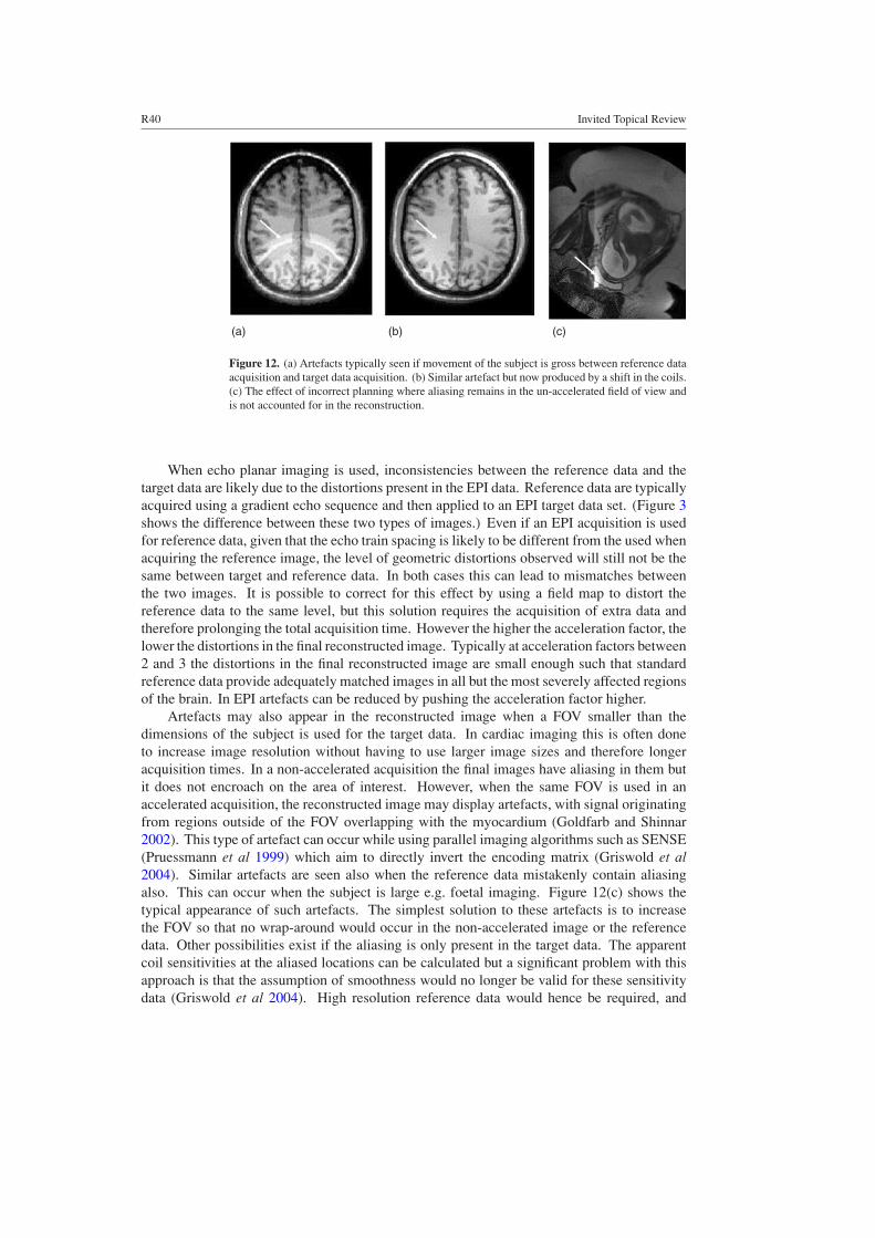
R40 Invited Topical Review
(a) (b) (c)
Figure 12. (a) Artefacts typically seen if movement of the subject is gross between reference dataacquisition and target data acquisition. (b) Similar artefact but now produced by a shift in the coils.(c) The effect of incorrect planning where aliasing remains in the un-accelerated field of view andis not accounted for in the reconstruction.
When echo planar imaging is used, inconsistencies between the reference data and thetarget data are likely due to the distortions present in the EPI data. Reference data are typicallyacquired using a gradient echo sequence and then applied to an EPI target data set. (Figure 3shows the difference between these two types of images.) Even if an EPI acquisition is usedfor reference data, given that the echo train spacing is likely to be different from the used whenacquiring the reference image, the level of geometric distortions observed will still not be thesame between target and reference data. In both cases this can lead to mismatches betweenthe two images. It is possible to correct for this effect by using a field map to distort thereference data to the same level, but this solution requires the acquisition of extra data andtherefore prolonging the total acquisition time. However the higher the acceleration factor, thelower the distortions in the final reconstructed image. Typically at acceleration factors between2 and 3 the distortions in the final reconstructed image are small enough such that standardreference data provide adequately matched images in all but the most severely affected regionsof the brain. In EPI artefacts can be reduced by pushing the acceleration factor higher.
Artefacts may also appear in the reconstructed image when a FOV smaller than thedimensions of the subject is used for the target data. In cardiac imaging this is often doneto increase image resolution without having to use larger image sizes and therefore longeracquisition times. In a non-accelerated acquisition the final images have aliasing in them butit does not encroach on the area of interest. However, when the same FOV is used in anaccelerated acquisition, the reconstructed image may display artefacts, with signal originatingfrom regions outside of the FOV overlapping with the myocardium (Goldfarb and Shinnar2002). This type of artefact can occur while using parallel imaging algorithms such as SENSE(Pruessmann et al 1999) which aim to directly invert the encoding matrix (Griswold et al2004). Similar artefacts are seen also when the reference data mistakenly contain aliasingalso. This can occur when the subject is large e.g. foetal imaging. Figure 12(c) shows thetypical appearance of such artefacts. The simplest solution to these artefacts is to increasethe FOV so that no wrap-around would occur in the non-accelerated image or the referencedata. Other possibilities exist if the aliasing is only present in the target data. The apparentcoil sensitivities at the aliased locations can be calculated but a significant problem with thisapproach is that the assumption of smoothness would no longer be valid for these sensitivitydata (Griswold et al 2004). High resolution reference data would hence be required, and
Invited Topical Review R41
are generally not available. A second possibility would be to alter the basic reconstructionequations to account for the extra-aliasing; this effectively increases the acceleration factorused in the reconstruction. While using full FOV reference data, the g-factor noise can stillbe kept under control using SENSE as suggested by Winkelmann et al (2005b). The imageis reconstructed once to estimate, through filtering, a body coverage map. This mask is thenapplied to the sensitivity data so as to exclude any background voxels from the reconstruction.As the number of overlapping aliases is reduced, so is noise amplification.
Any detrimental consequences to using reduced FOV reference data can be avoided byusing the approximate reconstruction algorithms, SMASH (Sodickson and Manning 1997) orGRAPPA (Griswold et al 2002), which try to recover the missing k-space information usingthe neighbouring k-space points instead. These methods are effective because the relationshipbetween the k-space data at each point is not inherently altered by choosing a smaller FOV(Griswold et al 2004).
3.4. The hardware
3.4.1. System requirements. As discussed in the introduction, the theoretical frameworkfor PI was proposed in the late 1980s but there was a delay in its widespread adoption duethe lack of multi-channel machines. After the widespread adoption of array coils to increaseSNR for large FOV imaging, the principles of which are outlined in Roemer’s paper (Roemeret al 1990), then the essential hardware for PI was in place. The receiver chain for thesemulti-channel machines remains to this day largely as described in Roemer’s paper. The mainimpact that PI has had on MR systems is the proliferation of channels and the design of coilsto use these channels.
Optimal SNR in most applications delivers diminishing returns as the number ofindependent receivers increases. Generally (a gross generalization!) a system with betweenfour and eight channels yields a good performance and hence commercial systems beforePI were usually sold with these many channels. PI quickly demonstrated that, even formodest accelerations of 2–4 at field strengths of 1.5–3.0 T, many more channels are requiredto overdetermine the system and produce numerically stable reconstructions with a smallg-factor. Having eight channels rapidly became a minimum requirement rather than an upperlimit.
Due to g-factor, accelerations are generally limited to 2–3 at currently used field strengths.Given this, a simple assessment might conclude that eight channels would be sufficient toprovide this level of acceleration with enough overdetermination of the reconstruction to keepit accurate. However, in general the coils do not have the ideal geometry with respect to thedesired field of view: they are not arranged as linear arrays with the principal direction ofvariation commensurate with the acceleration direction. For this to be the case, the phaseencode direction in all imaging exams would be dictated by the coil geometry rather than theanatomy of interest. If the imaging plane is rotated away from the optimal direction in a lineararray, the image quality will drop due to the unfavourable geometry. We can therefore see thatthe choice of imaging plane w.r.t. coils is critical. Taking the example of a cardiac application,this becomes clear where short and long axis views of the heart are inevitably double obliquedw.r.t. the magnet axes. To maintain the g-factor for all imaging planes in such an applicationis a major challenge. A key component is to increase the number of coils so that for any givenimaging plane there is a subset of coils which provide a well-conditioned reconstruction. Inthe torso this has been achieved with 2D arrays (Hardy et al 2004). In the brain a numberof designs have been proposed. Current coil designs are looking at using 32, 64 or even128 channels to try and achieve this flexibility.
R42 Invited Topical Review
Two principle system challenges arise from an increase in channel numbers: how tohandle the large increase in data throughput and how to manage the increase in cabling thatis commensurate with a large volume of coils. Data throughputs of 20 MB s−1 have beenreported for a 16-channel system which, for rapid imaging protocols can quickly lead tovery large sets of data (Bodurka et al 2004). A 40 min fMRI scan would easily result inraw data exceeding 40 GB per subject. With 32-channel systems this could double. Afterimage reconstruction the raw data will generally be reduced by a factor of the number ofcoils, but the reconstruction process will need to handle this volume and flow of data (Hardyet al 2004). Moore’s law has been of considerable help with increasing computational speedhelping maintain tolerable throughputs. The reconstruction processes themselves are highlyparallelizable at multiple graining levels, on a volume by volume basis, slice by slice basisand, for image domain reconstructions, on a pixel group by pixel group level. One researchgroup has dedicated a ten-node Linux-based ‘Beowulf’ processing cluster (Niendorf et al2006) to explore the use of parallel computing for parallel reconstruction. The widespreadavailability of 64 bit computing is making addressing of large amounts of memory possiblewhile also making an impact on the ability to reconstruct these large data sets. Even with allthis development, real-time reconstruction is still a challenge for systems with large numbersof array coils and both the research community and the manufacturers are working on thisproblem.
The mechanical architecture changes required to accommodate the large number ofelectrical connections from large numbers of coils are also proving challenging. Space insidethe bore of the magnet is at a premium and so embedding cabling (and sometimes coils) inthe patient handling mechanisms is one approach. Optical coupling has been suggested andtime domain multiplexing has been a longstanding approach used to maximize the use offewer receive chains (Bankson et al 2000). However, multiplexing is generally thought tocompromise SNR too much to be anything other than a transitional technology.
PI has not produced a conceptual paradigm shift in MR system hardware but has provokeda step up in the computation power systems now need to carry with them.
3.4.2. Coil design. Coil design is an area where PI has had a huge impact. It rapidly becameclear that the design criteria for an array coil used for optimal SNR imaging and one for PImight be different. At this point coil design could have diverged with some arrays beingspecifically designed for PI and some specifically designed for SNR. However it is generallyacknowledged that coils should perform well under both paradigms and so the more extremePI coil designs which improved g-factor at great expense of baseline SNR were not generallyadopted (Ohliger et al 2005). A full discussion of coil design is beyond the scope of thisreview and we would refer the interested reader to a review article by Ohliger and Sodickson(2006). We will discuss the features of array coils and some criteria for assessing successfulcoil design.
A coil consists of a conducting loop which is tuned to be resonant across the small range offrequencies it is expected to operate at (dictated by the Larmor frequency and hence the mainfield strength). The tuning is achieved by a combination of lumped components (capacitorsand inductors) and the contribution made by the body when it is in close proximity. The coilis then coupled to a pre-amplifier, usually built into the coil to add gain as close to the sourceas possible. This amplified signal is then streamed into an analogue-to-digital converter.
A consequence of the intimate interaction between coil and subject is that its performancevaries depending on the electromagnetic properties of the subject. This variation increases withincreasing field strength due to the reduction in wavelength producing small scale variationsin sensitivity along with global scaling seen at lower field strengths. If the performance of the

Invited Topical Review R43
coil varies on a subject by subject basis, then the calibration procedure required by PI mustalso be subject dependent even for a rigid, static coil.
When two or more surface coils are to be combined into an array then inductive couplingof the elements occurs. Coupling between elements is undesirable for two reasons. Firstly,if no explicit account is made of the coupling, the SNR is reduced in both optimal SNR andPI applications. The former because the assumption that signal is correlated across coils andnoise is not, is violated, and the latter because coil sensitivities are less independent reducingthe condition of the matrix inversion and therefore increasing g-factor noise unless explicitlyaccounted for. The second reason is that coil coupling introduces parasitic inductance andcapacitance into the coils circuit and so can detune the coil reducing its overall effectiveness.This can be offset in a fixed geometry as the coils can be tuned appropriately allowing for thecoupling, but if flexible placement of coils is required then an effective decoupling strategy isneeded which is not geometry dependent.
There are two widely used decoupling strategies. The first, which until recently was themost widely used, is geometrical decoupling where neighbouring loops are overlapped suchthat the mutual inductance between loops is exactly cancelled by the overlapping region. Thisis capable of providing exact decoupling for two or three loops (three loops arranged as a cloverleaf). Loops beyond this nearest-neighbour geometry are not decoupled. Often it is enoughto assume that the level of coupling from non-nearest-neighbour loops is insignificant due tothe distance between them. The second method to isolate coils is to increase the impedance ofthe pre-amplifiers such that the current in the coil is minimized (and therefore the coupling)without reducing the voltage (and therefore the signal). Pre-amplifier decoupling is now widelyused and enables more flexible coil geometries enabling the free placement of coil elements.However, decoupling is never perfect and to minimize its impact correlations between coilsshould be measured on a study by study basis and included in the reconstruction process asdescribed in the algorithm section of this review. The aim for freely positionable coils (orfreely positionable groups of coils) is to provide sufficient decoupling via the pre-amplifiersthat the impact on efficiency of the coils is small.
A major change in hardware, attributable almost entirely to PI, has been the acceptanceof array coils for imaging the head. Up until PI it was widely accepted that the birdcage coilwas close to optimal for imaging the brain as it provides almost optimal SNR over the wholebrain. It also has a uniform receive field resulting in images with uniform signal-to-noise ratioacross them rendering them easy to interpret. Unfortunately, the birdcage coil is not usefulfor PI as the receive fields of its two quadrature elements do not vary in space. So array coilshave largely superseded the birdcage.
Given that we know array coils are required for PI, and that the main feature we require isa spatially varying sensitivity, how might the optimal design problem be approached? Whenconsidering coil design what we are really looking at is how well does the array perform inunfolding an aliased image. Assessment of this is made by considering the impact of thereconstruction algorithm on the final image. For coil design we generally assume that thecoil sensitivity map can be exactly measured (this excludes the range of artefacts associatedwith inconsistency between reference and target data). We are then left with SNR as an imagequality metric. An assumption is also made that the effects of the body loading of the coilcan be approximated by assuming a standard load. The variations induced by the populationvariation, whilst significant enough to critically affect calibration, are assumed to have minimalimpact on the macroscopic coil design. This assumption is necessary unless coils are tailormade for each subject, an impractical approach.
Unlike imaging with uniform receive field coils (birdcages), arrays produce images withnon-uniform signal to noise. Disregarding PI it is clear that figure 5 has a varying signal level
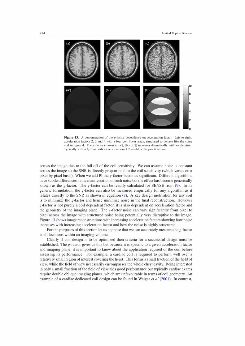
R44 Invited Topical Review
(a) (b) (c)
(a,) (b
,) (c
,)
Figure 13. A demonstration of the g-factor dependence on acceleration factor. Left to right,acceleration factors 2, 3 and 4 with a four-coil linear array, simulated to behave like the spinecoil in figure 4. The g-factor (shown in (a′), (b′), (c′)) increases dramatically with acceleration.Typically with only four coils an acceleration of 2 would be the practical limit.
across the image due to the fall off of the coil sensitivity. We can assume noise is constantacross the image so the SNR is directly proportional to the coil sensitivity (which varies on apixel by pixel basis). When we add PI the g-factor becomes significant. Different algorithmshave subtle differences in the manifestation of such noise but the effect has become genericallyknown as the g-factor. The g-factor can be readily calculated for SENSE from (9). In itsgeneric formulation, the g-factor can also be measured empirically for any algorithm as itrelates directly to the SNR as shown in equation (8). A key design motivation for any coilis to minimize the g-factor and hence minimize noise in the final reconstruction. Howeverg-factor is not purely a coil dependent factor, it is also dependent on acceleration factor andthe geometry of the imaging plane. The g-factor noise can vary significantly from pixel topixel across the image with structured noise being potentially very disruptive to the image.Figure 13 shows image reconstructions with increasing acceleration factors showing how noiseincreases with increasing acceleration factor and how the noise is highly structured.
For the purposes of this section let us suppose that we can accurately measure the g-factorat all locations within an imaging volume.
Clearly if coil design is to be optimized then criteria for a successful design must beestablished. The g-factor gives us this but because it is specific to a given acceleration factorand imaging plane, it is important to know about the application required of the coil beforeassessing its performance. For example, a cardiac coil is required to perform well over arelatively small region of interest covering the heart. This forms a small fraction of the field ofview, while the field of view necessarily encompasses the whole chest cavity. Being interestedin only a small fraction of the field of view aids good performance but typically cardiac examsrequire double oblique imaging planes, which are unfavourable in terms of coil geometry. Anexample of a cardiac dedicated coil design can be found in Weiger et al (2001). In contrast,
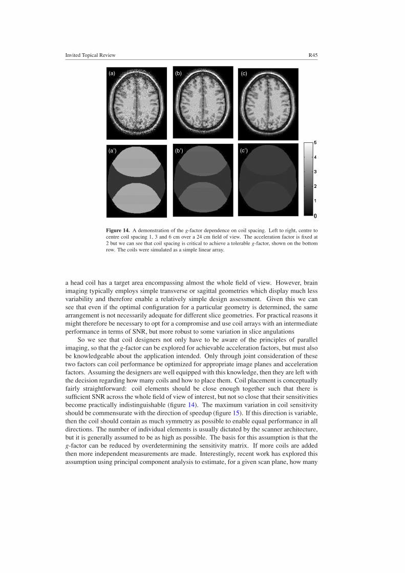
Invited Topical Review R45
(a) (b) (c)
(a,) (b
,) (c
,)
Figure 14. A demonstration of the g-factor dependence on coil spacing. Left to right, centre tocentre coil spacing 1, 3 and 6 cm over a 24 cm field of view. The acceleration factor is fixed at2 but we can see that coil spacing is critical to achieve a tolerable g-factor, shown on the bottomrow. The coils were simulated as a simple linear array.
a head coil has a target area encompassing almost the whole field of view. However, brainimaging typically employs simple transverse or sagittal geometries which display much lessvariability and therefore enable a relatively simple design assessment. Given this we cansee that even if the optimal configuration for a particular geometry is determined, the samearrangement is not necessarily adequate for different slice geometries. For practical reasons itmight therefore be necessary to opt for a compromise and use coil arrays with an intermediateperformance in terms of SNR, but more robust to some variation in slice angulations
So we see that coil designers not only have to be aware of the principles of parallelimaging, so that the g-factor can be explored for achievable acceleration factors, but must alsobe knowledgeable about the application intended. Only through joint consideration of thesetwo factors can coil performance be optimized for appropriate image planes and accelerationfactors. Assuming the designers are well equipped with this knowledge, then they are left withthe decision regarding how many coils and how to place them. Coil placement is conceptuallyfairly straightforward: coil elements should be close enough together such that there issufficient SNR across the whole field of view of interest, but not so close that their sensitivitiesbecome practically indistinguishable (figure 14). The maximum variation in coil sensitivityshould be commensurate with the direction of speedup (figure 15). If this direction is variable,then the coil should contain as much symmetry as possible to enable equal performance in alldirections. The number of individual elements is usually dictated by the scanner architecture,but it is generally assumed to be as high as possible. The basis for this assumption is that theg-factor can be reduced by overdetermining the sensitivity matrix. If more coils are addedthen more independent measurements are made. Interestingly, recent work has explored thisassumption using principal component analysis to estimate, for a given scan plane, how many
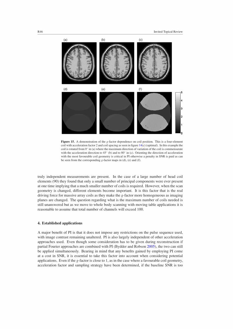
R46 Invited Topical Review
(a) (b) (c)
(d) (e) (f )
Figure 15. A demonstration of the g-factor dependence on coil position. This is a four-elementcoil with acceleration factor 2 and coil spacing as seen in figure 14(c) (optimal). In this example thecoil is rotated from 0◦ in (a) where the maximum direction of variation of the coil is commensuratewith the acceleration direction to 45◦ (b) and to 80◦ in (c). Orienting the direction of accelerationwith the most favourable coil geometry is critical in PI otherwise a penalty in SNR is paid as canbe seen from the corresponding g-factor maps in (d), (e) and (f).
truly independent measurements are present. In the case of a large number of head coilelements (90) they found that only a small number of principal components were ever presentat one time implying that a much smaller number of coils is required. However, when the scangeometry is changed, different elements become important. It is this factor that is the realdriving force for massive array coils as they make the g-factor more homogeneous as imagingplanes are changed. The question regarding what is the maximum number of coils needed isstill unanswered but as we move to whole body scanning with moving table applications it isreasonable to assume that total number of channels will exceed 100.
4. Established applications
A major benefit of PI is that it does not impose any restrictions on the pulse sequence used,with image contrast remaining unaltered. PI is also largely independent of other accelerationapproaches used. Even though some consideration has to be given during reconstruction ifpartial Fourier approaches are combined with PI (Bydder and Robson 2005), the two can stillbe applied simultaneously. Bearing in mind that any benefits gained by employing PI comeat a cost in SNR, it is essential to take this factor into account when considering potentialapplications. Even if the g-factor is close to 1, as in the case where a favourable coil geometry,acceleration factor and sampling strategy have been determined, if the baseline SNR is too
Invited Topical Review R47
low (SNRfull in (8)), the reconstructed image may not have any diagnostic value after the SNRreduction resulting from the application of PI.
Obvious clinical applications are therefore those for which a high signal is inherentlyavailable. (EPI is potentially an exception to this which we will discuss separately.) Alongsidethis consideration, are applications where currently the acquisition speed is limited by thegradient performance. Generally these are methods where high temporal resolution is neededbut the rapid acquisition methods currently employed are still not fast enough to capture allkey information. PI is now integrated into many routine MR exams. The following sectiondiscusses a few key applications and describes what makes them good targets for PI. The listis clearly not exhaustive but it is hoped that it will give the reader an insight into how goodapplications can be identified.
3D acquisitions are an excellent target for PI. In a 2D acquisition one slice is excitedat a time and phase encoding is performed along one of the in-plane directions. Instead ofrepeating this procedure for a set of slices, a 3D alternative is to excite a whole slab andperform phase encoding also along what would otherwise be the slice select direction. Toreconstruct the image a 3D Fourier transform is then required instead of a 2D Fourier transform.3D acquisitions are generally more time consuming than 2D acquisitions but bring with themmuch better 3D visualization with artefact free multi-planar reformatted images. Reformattingis useful for many applications, for example vessel wall imaging where the tortuous routes ofvessels make it essential for viewing. Whole brain survey scans are also generally 3D. Thelong scan times associated with 3D imaging make these scans an attractive proposition for PI.In addition in 3D imaging there are two orthogonal directions of phase encoding and so PI canbe applied in both directions (Weiger et al 2002). When (in this case regular) sub-sampling isapplied in 2D, the aliasing pattern results in the distance between aliased pixels being greaterthan if the same speedup factor is applied in only one dimension (figure 16). This changein sampling pattern improves the g-factor allowing greater acceleration factors provided thecoils used have varying sensitivity in both directions. This is almost always the case in headimaging but is less likely in the body.
Angiography is an area where PI is now widely used, particularly 3D contrast enhancedangiography (Weiger et al 2000b). Alongside the suitability of 3D acquisitions discussedabove, contrast enhanced studies are particularly suited for PI due to the high SNR madeavailable through the application of the contrast agent.
When applying PI to MR contrast enhanced angiography (MRCEA), the extra informationprovided by the coils can be used to increase the spatial resolution, improving the ability tovisualize, for example, small vessels. Alternatively, the spatial resolution can be maintained,and the temporal resolution improved instead. In this way a better estimate of when the contrastreaches individual vessels can be obtained. The use of parallel imaging may also contributeto reducing sensitivity to artefacts. An example is a reduction in venous contamination as aresult of shorter acquisition times. This is particularly a problem in regions where the venousreturn is very rapid such as the renal and carotid arteries. The same effect can be reduced whenimaging the lower parts of the body. In order to follow the path of the contrast agent, theseareas are normally imaged last. Reducing the acquisition time therefore reduces the likelihoodthat the contrast agent may already have reached the veins in this part of the body. In contrastenhanced acquisitions the intrinsic SNR is linked to the concentration of the contrast agentand so any loss in SNR may be partially compensated for by increasing the contrast bolus.
Non-contrast-based angiographic techniques also benefit from PI. Both time of flight,where inflow is used to preferentially select blood signal and phase contrast angiographywhere the flowing blood accumulates phase (PCA) are high contrast high SNR 3D methods.Figure 17 shows an example of a PCA acquisition accelerated with a factor of 2 and 3. The
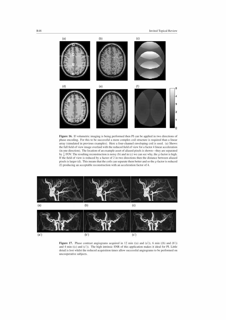
R48 Invited Topical Review
(a) (b) (c)
(d) (e) (f )
Figure 16. If volumetric imaging is being performed then PI can be applied in two directions ofphase encoding. For this to be successful a more complex coil structure is required than a lineararray (simulated in previous examples). Here a four-channel enveloping coil is used. (a) Showsthe full field of view image overlaid with the reduced field of view for a factor 4 linear acceleration(in one direction). The location of an example asset of aliased pixels is shown—they are separatedby 1
4 FOV. The resulting reconstruction is noisy (b) and in (c) we can see why, the g-factor is high.If the field of view is reduced by a factor of 2 in two directions then the distance between aliasedpixels is larger (d). This means that the coils can separate them better and so the g-factor is reduced(f) producing an acceptable reconstruction with an acceleration factor of 4.
(a) (b) (c)
(a,) (b
,) (c
,)
Figure 17. Phase contrast angiograms acquired in 12 min ((a) and (a′)), 6 min ((b) and (b′))and 4 min ((c) and (c′)). The high intrinsic SNR of this application makes it ideal for PI. Littledetail is lost whilst the reduced acquisition times allow successful angiograms to be performed onuncooperative subjects.

Invited Topical Review R49
impact on image quality is minimal while the reduction of scan time from 12 to 4 min iscritical in achieving motion free data, particularly from uncooperative patients and infants.The small impact in image quality due to acceleration in figure 17 is typical of phase contrastangiography, time of flight angiography and contrast enhanced angiography.
When imaging the chest or abdomen, motion artefact due to respiratory motion is a majorproblem. Typically the respiratory cycle lasts approximately 4 s and most scan times are far inexcess of this. Rapid imaging techniques which employ echo trains have limited resolution,and the large size of the body makes them particularly unsuitable in these areas. Typically acompromise is reached, with the patients being asked to hold their breath during an acquisitionthat lasts between 5 and 20 s depending on their ability. PI allows breath-holds to be madeshorter and therefore much more tolerable for patients. This significantly helps to reducemotion-related artefacts in the images. Imaging the heart is very challenging due to motionrelated to both the cardiac and respiratory cycles (Pruessmann et al 2001a, Jakob et al 1999).In order to improve image resolution, the acquisition needs to be lengthened. Unfortunately,if the tissue moves by a significant distance during this time, the actual resolution achievedis reduced due to blurring and artefacts. Using parallel imaging, a higher spatial resolutioncan be achieved without having to increase the acquisition time any further. Alternatively, thetemporal resolution can be improved instead, allowing us to better study the dynamics of heartfunction. The possibility to speedup the acquisition also has a significant impact regardingcardiac triggering. As the number of cycles required to complete an image is reduced, thelikelihood of obtaining useful data significantly improves for patients for which triggering isdifficult, e.g. in the presence of arrhythmias. In extreme cases it is possible to resort to real-time imaging, which does not require any sort of gating (Weiger et al 2000a). The dynamicsof individual cycles can be captured by significantly reducing the acquisition time per frame.Using parallel imaging this can be done without excessively compromising spatial resolution.
In many neuro applications such as functional MRI (fMRI) or diffusion-weighted imaging(DWI), single-shot EPI is the standard imaging technique. In fMRI this is because of thetemporal resolution required to capture rapid haemodynamic changes which are associatedwith the change in the magnetic properties of blood in the transition from deoxy- to oxy-haemoglobin during brain activation. In diffusion-weighted imaging, images are madesensitive to the diffusion of water molecules. In order to make the images sufficiently sensitiveto detect the very fine motion of these molecules, they necessarily become very sensitive tobulk patient motion as well. This may lead to data inconsistency if multi-shot techniques areused. Scanning times also need to be kept as short as possible so as to enable the acquisitionof multiple diffusion-weighted image volumes as required to estimate diffusion anisotropy.
Unfortunately, although EPI is critical to making such applications work it does presentsignificant limitations precisely because all of the data are acquired following a single RFexcitation. Figure 3 shows a typical EPI image compared to a GRE acquisition. Afterexcitation, the signal progressively decays due to relaxation, and for this reason the numberof echoes which can be acquired before the signal becomes indistinguishable from noise iseffectively limited. For a fixed FOV, this means that the extent of k-space sampled, and hencethe image resolution attained, is necessarily limited. Another consequence of signal decayis the introduction of blurring in the image, which reduces the effective resolution achieved.This is due to the reduced signal at the edges of k-space. An added problem of having longerecho trains is that there is more time for any phase errors to accumulate, resulting in artefactsin the image. EPI images are hence very sensitive to off-resonance effects (imperfections inthe main magnetic field, either intrinsic to the magnet or induced by the presence of a subjectwith finite magnetic susceptibility). Geometric distortions can therefore be seen in some areasof the brain, such as the frontal lobe, where the field is less homogeneous due to the sinus air
R50 Invited Topical Review
space. This is because the extra phase resulting from differences in resonance frequency isinterpreted as being due to a different spatial location within the brain. The displacement errorin pixel units depends on both the difference in frequency �ω and the time interval betweenconsecutive echoes—the inter-echo spacing (�TE):
�rPE = �ω · �T E. (30)
The displacement errors are significant only along the phase encode direction, as the timebetween the acquisition of two consecutive points in k-space is much longer along this direction.When PI is used, because missing k-space lines are reconstructed from surrounding lines, theeffective inter-echo spacing is reduced, reducing distortions.
Another type of artefact visible in EPI is the presence of a distribution of frequenciesalong the slice direction due once again to field inhomogeneities. In this case intra-voxeldephasing leads to a local decrease in image intensity. The total signal loss is proportional tothe time the spin system is exposed to the dephasing fields. This effect is reduced using PI asthe echo train length is reduced.
Because the signal in EPI decays as a function of echo position, it is possible that evenif the same resolution is maintained, reducing the echo train length may actually lead to anoverall improvement in SNR as a result of a shorter echo time. This improvement is dependenton the T2 of the tissue: the shorter the T2 the greater the benefit in SNR from PI, while longT2 compartments suffer loss in SNR (Jaermann et al 2004).
Because of these factors the application of parallel imaging to EPI applications iswidespread. The result is a significant reduction in the level of geometric distortions, signaldropout, and blurring artefacts and a potential increase in SNR. PI has been very successfulin both fMRI (Golay et al 2000) and DWI (Jaermann et al 2004, Bammer et al 2001). Areduction in geometric distortions which can be enabled using PI has also been shown to bebeneficial to DTI (Andersson et al 2004). All of these techniques have EPI as their basis.
5. Emerging applications
The principle behind all PI applications is that when imaging with localized coils we havegenerally a surplus of measurements. This surplus can be used to accelerate the acquisition orcould be used for other purposes. So far the use of coil information for purposes other thanaccelerating imaging has focused on two areas: the removal of coherent image domain artefactswhich were not caused by aliasing, and improving image quality by tackling inconsistenciesintroduced in MR data due to motion during the acquisition. A review of motion correctionmethods can be found in Larkman et al (2004). In either application the concept of dataconsistency is used to modify the image reconstruction so as to make the final image onewhich is consistent with the object.
Motion correction using PI exploits the excess of information in an overdetermined dataset. Conceptually the most accessible method that has been proposed is known as SMASHnavigation (Bydder et al 2003). In this method the SMASH formalism is used to generate anew prediction of a line in k-space which is compared to the actual measured line. This systemallows us to determine if motion has occurred between the acquisition of these two lines.If the prediction and the actual measured line are the same within error then no motion hasoccurred. If they are different then the difference is assigned to motion and the data can eitherbe corrected (using an iterative fit for known simple motion parameters) or it can be rejected(Bydder et al 2002b), and the generated line used in its place. This can then be propagatedacross k-space to produce a self-consistent image. This method is limited in that only simplecorrections can be applied such as simple rotations, rigid body motion, etc. As these clearly
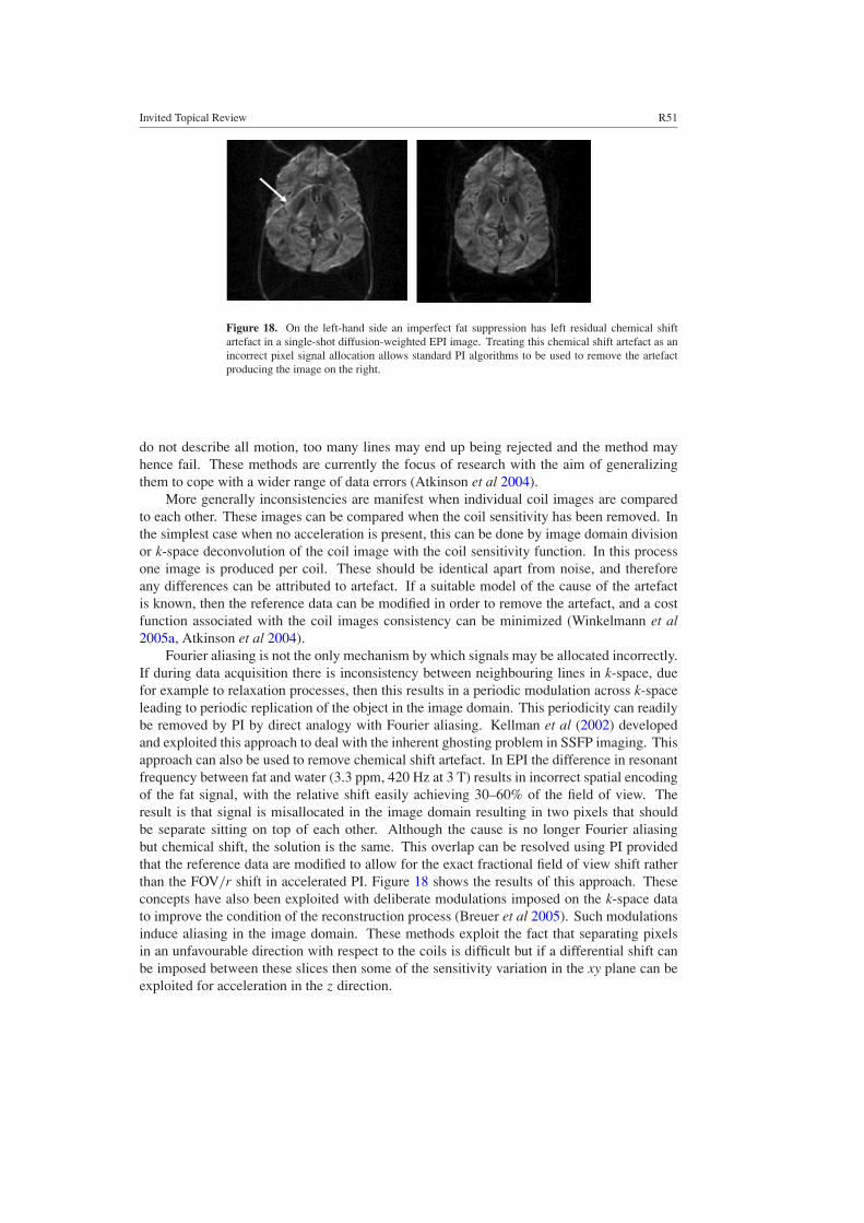
Invited Topical Review R51
Figure 18. On the left-hand side an imperfect fat suppression has left residual chemical shiftartefact in a single-shot diffusion-weighted EPI image. Treating this chemical shift artefact as anincorrect pixel signal allocation allows standard PI algorithms to be used to remove the artefactproducing the image on the right.
do not describe all motion, too many lines may end up being rejected and the method mayhence fail. These methods are currently the focus of research with the aim of generalizingthem to cope with a wider range of data errors (Atkinson et al 2004).
More generally inconsistencies are manifest when individual coil images are comparedto each other. These images can be compared when the coil sensitivity has been removed. Inthe simplest case when no acceleration is present, this can be done by image domain divisionor k-space deconvolution of the coil image with the coil sensitivity function. In this processone image is produced per coil. These should be identical apart from noise, and thereforeany differences can be attributed to artefact. If a suitable model of the cause of the artefactis known, then the reference data can be modified in order to remove the artefact, and a costfunction associated with the coil images consistency can be minimized (Winkelmann et al2005a, Atkinson et al 2004).
Fourier aliasing is not the only mechanism by which signals may be allocated incorrectly.If during data acquisition there is inconsistency between neighbouring lines in k-space, duefor example to relaxation processes, then this results in a periodic modulation across k-spaceleading to periodic replication of the object in the image domain. This periodicity can readilybe removed by PI by direct analogy with Fourier aliasing. Kellman et al (2002) developedand exploited this approach to deal with the inherent ghosting problem in SSFP imaging. Thisapproach can also be used to remove chemical shift artefact. In EPI the difference in resonantfrequency between fat and water (3.3 ppm, 420 Hz at 3 T) results in incorrect spatial encodingof the fat signal, with the relative shift easily achieving 30–60% of the field of view. Theresult is that signal is misallocated in the image domain resulting in two pixels that shouldbe separate sitting on top of each other. Although the cause is no longer Fourier aliasingbut chemical shift, the solution is the same. This overlap can be resolved using PI providedthat the reference data are modified to allow for the exact fractional field of view shift ratherthan the FOV/r shift in accelerated PI. Figure 18 shows the results of this approach. Theseconcepts have also been exploited with deliberate modulations imposed on the k-space datato improve the condition of the reconstruction process (Breuer et al 2005). Such modulationsinduce aliasing in the image domain. These methods exploit the fact that separating pixelsin an unfavourable direction with respect to the coils is difficult but if a differential shift canbe imposed between these slices then some of the sensitivity variation in the xy plane can beexploited for acceleration in the z direction.

R52 Invited Topical Review
6. Discussion
Parallel imaging has really been a developing story ever since the late 1980s. Whilst thereare many different reconstruction methods for PI there is much commonality. The simplereconstruction methods are generally the most robust and computationally efficient. Forregular undersampled k-space with low acceleration factors and well-designed coils all themethods largely produce the same result. If more ambitious k-space trajectories or non-uniformundersampling is required, then differences become apparent. It is when the algorithms arepushed e.g. high acceleration factors or inconsistent reference data are used that differentalgorithms have different SNR properties and/or artefacts. Ultimately all the schemes arecombining the signal from multiple coils in a linear way.
The choice between auto-calibration and separate calibration of coils should be applicationdriven. Separate calibration has been proven to be robust in all cases except where extrememotion is present. Generally the coil calibration is relatively straightforward and has now beenassimilated in the standard clinical protocol in the same way that other essential calibrations(RF power, shim, etc) are, as calibration data can typically be acquired for a full imagingvolume in 30–60 s. These data can then be used for all subsequent acquisitions provided thepatient and/or coils do not move.
As with all imaging techniques there are some methodology-specific artefacts thatradiologists need to be aware of so that on the rare occasions they do appear they are notmistaken for pathology. PI artefacts are usually easily recognizable due to their linking ofremote regions of the image.
It is interesting to note that all the main manufacturers Philips, Siemens and GE haveadopted PI in one form or another. It has been integrated into the core product very rapidly.Naturally they have adopted SENSE or SMASH (GRAPPA) like methods due to the speed ofreconstruction but we should expect to see other algorithms also adopted in the near futureto allow non-Cartesian accelerated acquisitions. PI has provided a bonanza for coil designersand as generally all but the basic head coils are optional extras on MR, this has given thedevelopment of PI a major commercial incentive.
Newer ideas surrounding artefact suppression using PI have yet to take hold commercially,their utility is still being tested in the research community but it is inevitable that they willemerge eventually.
Conceptually PI shares common ground with radar and telecommunications technologies.Antenna arrays are common in many areas of physics but the near field nature of the MRproblem has meant that it has been largely developed separately so far. As the MR applicationbecomes more mature we will no doubt see more cross fertilization between these areasparticularly with the development of transmit arrays combined with receiver arrays bringingan obvious link with multiple-input multiple-output (Mimo) technology now employed inshort and long range wireless communications.
References
Adriany G et al 2005 Transmit and receive transmission line arrays for 7 Tesla parallel imaging Magn. Reson.Med. 53 434–45
Andersson J, Richter M, Richter W, Skare S, Nunes R, Robson M and Behrens T 2004 Effects of susceptibilitydistortions on tractography 12th Annual Meeting of ISMRM (Kyoto, Japan)
Atkinson D, Larkman D J, Batchelor P G, Hill D L and Hajnal J V 2004 Coil-based artifact reduction Magn. Reson.Med. 52 825–30
Bammer R, Keeling S L, Augustin M, Pruessmann K P, Wolf R, Stollberger R, Hartung H P and Fazekas F2001 Improved diffusion-weighted single-shot echo-planar imaging (EPI) in stroke using sensitivity encoding(SENSE) Magn. Reson. Med. 46 548–54
Invited Topical Review R53
Bankson J A, Griswold M A, Wright S M and Sodickson D K 2000 SMASH imaging with an eight element multiplexedRF coil array Magma 10 93–104
Bodurka J, Ledden P J, van Gelderen P, Chu R, de Zwart J A, Morris D and Duyn J H 2004 Scalable multichannelMRI data acquisition system Magn. Reson. Med. 51 165–71
Breuer F A, Blaimer M, Heidemann R M, Mueller M F, Griswold M A and Jakob P M 2005 Controlled aliasingin parallel imaging results in higher acceleration (CAIPIRINHA) for multi-slice imaging Magn. Reson.Med. 53 684–91
Bydder M, Atkinson D, Larkman D J, Hill D L and Hajnal J V 2003 SMASH navigators Magn. Reson.Med. 49 493–500
Bydder M, Larkman D J and Hajnal J V 2002a Combination of signals from array coils using image-based estimationof coil sensitivity profiles Magn. Reson. Med. 47 539–48
Bydder M, Larkman D J and Hajnal J V 2002b Detection and elimination of motion artifacts by regeneration ofk-space Magn. Reson. Med. 47 677–86
Bydder M, Larkman D J and Hajnal J V 2002c Generalized SMASH imaging Magn. Reson. Med. 47 160–70Bydder M and Robson M D 2005 Partial Fourier partially parallel imaging Magn. Reson. Med. 53 1393–401Carlson J W 1987 An algorithm for NMR imaging reconstruction based on multiple Rf receiver coils J. Magn. Reson.
74 376–80Carlson J W and Minemura T 1993 Imaging time reduction through multiple receiver coil data acquisition and
image-reconstruction Magn. Reson. Med. 29 681–8de Zwart J A, Ledden P J, Kellman P, van Gelderen P and Duyn J H 2002 Design of a SENSE-optimized high-
sensitivity MRI receive coil for brain imaging Magn. Reson. Med. 47 1218–27Golay X, Pruessmann K P, Weiger M, Crelier G R, Folkers P J, Kollias S S and Boesiger P 2000 PRESTO-SENSE:
an ultrafast whole-brain fMRI technique Magn. Reson. Med. 43 779–86Goldfarb J W and Shinnar M 2002 Field-of-view restrictions for artifact-free SENSE imaging 10th Annual Meeting
of ISMRM (Honolulu, USA)Griswold M A, Jakob P M, Heidemann R M, Nittka M, Jellus V, Wang J, Kiefer B and Haase A 2002 Generalized
autocalibrating partially parallel acquisitions (GRAPPA) Magn. Reson. Med. 47 1202–10Griswold M A, Jakob P M, Nittka M, Goldfarb J W and Haase A 2000 Partially parallel imaging with localized
sensitivities (PILS) Magn. Reson. Med. 44 602–9Griswold M A, Kannengiesser S, Heidemann R M, Wang J and Jakob P M 2004 Field-of-view limitations in parallel
imaging Magn. Reson. Med. 52 1118–26Haacke E, Brown R, Thompson M and Venkatesan R 1999 Magnetic resonance imaging Physical Principles and
Sequence Design (New York: Wiley)Hansen P 1998 Rank-Deficient and Discrete Ill-Posed Problems: Numerical Aspects of Linear Inversion (Philadelphia,
PA: SIAM)Hardy C J, Darrow R D, Saranathan M, Giaquinto R O, Zhu Y, Dumoulin C L and Bottomley P A 2004 Large
field-of-view real-time MRI with a 32-channel system Magn. Reson. Med. 52 878–84Haselgrove J and Prammer M 1986 An algorithm for compensation of surface-coil images for sensitivity of the surface
coil Magn. Reson. Imaging 4 469–72Hasse A, Frahm D and Mattaei 1989 Flash imaging: rapid NMR imaging using low flip angle pulses J. Magn. Reson.
67 388–97Heidemann R M, Griswold M A, Haase A and Jakob P M 2001 VD-AUTO-SMASH imaging Magn. Reson.
Med. 45 1066–74Hestenes M A S E 1952 Methods of conjugate gradients for solving linear systems J. Res. National Bureau Standards
49 409–36Hutchinson M and Raff U 1988 Fast MRI data acquisition using multiple detectors Magn. Reson. Med. 6 87–91Jaermann T et al 2004 SENSE-DTI at 3 T Magn. Reson. Med. 51 230–6Jakob P M, Griswold M A, Edelman R R, Manning W J and Sodickson D K 1999 Accelerated cardiac imaging using
the SMASH technique J. Cardiovasc. Magn. Reson. 1 153–7Jakob P M, Griswold M A, Edelman R R and Sodickson D K 1998 AUTO-SMASH: a self-calibrating technique for
SMASH imaging. SiMultaneous acquisition of spatial harmonics Magma 7 42–54Katscher U, Bornert P, Leussler C and van den Brink J S 2003 Transmit SENSE Magn. Reson. Med. 49 144–50Kellman P, Guttman M A, Herzka D A and McVeigh E R 2002 Phased array ghost elimination (PAGE) for segmented
SSFP imaging with interrupted steady-state Magn. Reson. Med. 48 1076–80King K and Angelos L 2001 SENSE imaging quality improvement using matrix regularization 9th Annual Meeting
of ISMRM (Glasgow, Scotland)Kwiat D, Einav S and Navon G 1991 A decoupled coil detector array for fast image acquisition in magnetic resonance
imaging Med. Phys. 18 251–65

R54 Invited Topical Review
Kyriakos W E, Hoge W S and Mitsouras D 2006 Generalized encoding through the use of selective excitation inaccelerated parallel MRI NMR Biomed. 19 379–92
Kyriakos W E, Panych L P, Kacher D F, Westin C F, Bao S M, Mulkern R V and Jolesz F A 2000 Sensitivityprofiles from an array of coils for encoding and reconstruction in parallel (SPACE RIP) Magn. Reson. Med.44 301–8
Larkman D J, Atkinson D and Hajnal J V 2004 Artifact reduction using parallel imaging methods Top. Magn. Reson.Imaging 15 267–75
Larkman D J, Batchelor P G, Atkinson D, Rueckert D and Hajnal J V 2006 Beyond the g-factor limit in sensitivityencoding using joint histogram entropy Magn. Reson. Med. 55 153–60
Larkman D J, DeSouza N M, Bydder M and Hajnal J V 2001 An investigation into the use of sensitivity-encodedtechniques to increase temporal resolution in dynamic contrast-enhanced breast imaging J. Magn. Reson.Imaging 14 329–35
Lin F H, Kwong K K, Belliveau J W and Wald L L 2004 Parallel imaging reconstruction using automatic regularizationMagn. Reson. Med. 51 559–67
Malik S J, Schmitz S, O’Regan D, Larkman D J and Hajnal J V 2006 x-f choice: reconstruction of undersampleddynamic MRI by data-driven alias rejection applied to contrast-enhanced angiography Magn. Reson. Med.56 811–23
Margosian P, Schmitt F and Purdy D 1986 Faster MR imaging: Imaging with half the data Health Care Instrum. 1195–7
McDougall M P and Wright S M 2005 64-channel array coil for single echo acquisition magnetic resonance imagingMagn. Reson. Med. 54 386–92
Niendorf T et al 2006 Toward single breath-hold whole-heart coverage coronary MRA using highly acceleratedparallel imaging with a 32-channel MR system Magn. Reson. Med. 56 167–76
Ohliger M A, Grant A K and Sodickson D K 2003 Ultimate intrinsic signal-to-noise ratio for parallel MRI:electromagnetic field considerations Magn. Reson. Med. 50 1018–30
Ohliger M A, Greenman R L, Giaquinto R, Mckenzie C A, Wiggins G and Sodickson D K 2005 Concentric coilarrays for parallel MRI Magn. Reson. Med. 54 1248–60
Ohliger M A and Sodickson D K 2006 An introduction to coil array design for parallel MRI NMR Biomed. 19 300–15Panych L P and Jolesz F A 1994 A dynamically adaptive imaging algorithm for wavelet-encoded MRI Magn. Reson.
Med. 32 738–48Panych L P, Mulkern R V, Saiviroonporn P, Zientara G P and Jolesz F A 1997 Non-Fourier encoding with multiple
spin echoes Magn. Reson. Med. 38 964–73Pruessmann K P, Weiger M and Boesiger P 2001a Sensitivity encoded cardiac MRI J. Cardiovasc. Magn. Reson.
3 1–9Pruessmann K P, Weiger M, Bornert P and Boesiger P 2001b Advances in sensitivity encoding with arbitrary k-space
trajectories Magn. Reson. Med. 46 638–51Pruessmann K P, Weiger M, Scheidegger M B and Boesiger P 1999 SENSE: sensitivity encoding for fast MRI Magn.
Reson. Med. 42 952–62Roemer P B, Edelstein W A, Hayes C E, Souza S P and Mueller O M 1990 The NMR phased array Magn. Reson.
Med. 16 192–225Sodickson D K, Griswold M A, Jakob P M, Edelman R R and Manning W J 1999 Signal-to-noise ratio and signal-
to-noise efficiency in SMASH imaging Magn. Reson. Med. 41 1009–22Sodickson D K and Manning W J 1997 Simultaneous acquisition of spatial harmonics (SMASH): fast imaging with
radiofrequency coil arrays Magn. Reson. Med. 38 591–603Tikhonov A and Arsenin V 1977 Solutions of Ill-Posed Problems (New York: Wiley)Tsao J, Boesinger P and Pruessmann K P 2003 k-t BLAST and k-t SENSE: dynamic MRI with high frame rate
exploiting spatiotemporal correlations Magn. Reson. Med. 50 1031–43van Vaals J J, Brummer M E, Dixon W T, Tuithof H H, Engels H, Nelson R C, Gerety B M, Chezmar J L and
den Boer J A 1993 ‘Keyhole’ method for accelerating imaging of contrast agent uptake J. Magn. Reson.Imaging 3 671–5
Wang Z, Wang J and Detre J A 2005 Improved data reconstruction method for GRAPPA Magn. Reson. Med.54 738–42
Weiger M, Pruessmann K P and Boesiger P 2000a Cardiac real-time imaging using SENSE Magn. Reson.Med. 43 177–84
Weiger M, Pruessmann K P and Boesiger P 2002 2D SENSE for faster 3D MRI Magn. Reson. Mater. Phys. Biol.Med. 14 10–9
Weiger M, Pruessmann K P, Kassner A, Roditi G, Lawton T, Reid A and Boesiger P 2000b Contrast-enhanced 3DMRA using SENSE J. Magn. Reson. Imaging 12 671–7
Invited Topical Review R55
Weiger M, Pruessmann K P, Leussler C, Roschmann P and Boesiger P 2001 Specific coil design for SENSE: asix-element cardiac array Magn. Reson. Med. 45 495–504
Wiesinger F, Boesiger P and Pruessmann K P 2004a Electrodynamics and ultimate SNR in parallel MR imagingMagn. Reson. Med. 52 376–90
Wiesinger F, van de Moortele P F, Adriany G, de Zanche N, Ugurbil K and Pruessmann K P 2004b Parallel imagingperformance as a function of field strength—an experimental investigation using electrodynamic scaling Magn.Reson. Med. 52 953–64
Wiesinger F, van de Moortele P F, Adriany G, de Zanche N, Ugurbil K and Pruessmann K P 2006 Potential andfeasibility of parallel MRI at high field NMR Biomed. 19 368–78
Winkelmann R, Bornert P and Dossel O 2005a Ghost artifact removal using a parallel imaging approach Magn. Reson.Med. 54 1002–9
Winkelmann R, Bornert P, Nehrke K and Dossel O 2005b Efficient foldover suppression using SENSEMagma 18 63–8
Zientara G P, Panych L P and Jolesz F A 1994 Dynamically adaptive MRI with encoding by singular valuedecomposition Magn. Reson. Med. 32 268–74