PARALLEL NAVIER STOKES SOLUTIONS OF LOW ASPECT RATIO RECTANGULAR FLAT WINGS

IN COMPRESSIBLE FLOW

A DISSERTATION SUBMITTED TO THE GRADUATE SCHOOL OF NATURAL AND APPLIED SCIENCES

OF MIDDLE EAST TECHNICAL UNIVERSITY

BY

GÖKHAN DURMUŞ

IN PARTIAL FULFILLMENT OF THE REQUIREMENTS FOR

THE DOCTOR OF PHILOSOPHY IN

AEROSPACE ENGINEERING

SEPTEMBER 2004

Approval of the Graduate School Natural and Applied Sciences

Prof. Dr. Canan Özgen

Director

I certify that this thesis satisfies all the requirements as a thesis for the degree of Doctor of Philosophy.

Prof. Dr. Nafiz Alemdaroğlu Head of department

This is to certify that we have read this thesis and that in our opinion it is fully adequate, in scope and quality, as a thesis for the degree of Doctor of Philosophy. Prof. Dr. Mehmet Ş. Kavsaoğlu Assoc.Prof. Dr. Sinan Eyi Co-Supervisor Supervisor Examining Committee Members (first name belongs to the chairperson of the jury and the second name belongs to supervisor) Prof. Dr. Sinan Akmandor (METU, AE)

Assoc.Prof. Dr. Sinan Eyi (METU, AE)

Prof. Dr. Mehmet Ş. Kavsaoğlu (ITU, AE)

Prof. Dr. Ünver Kaynak (ETU, ME)

Assoc. Prof. Dr.Yusuf Özyörük (METU, AE)

iii

I hereby declare that all information in this document has been

obtained and presented in accordance with academic rules and ethical

conduct. I also declare that, as required by these rules and conduct, I

have fully cited and referenced all material and results that are not

original to this work.

Name, Last name : Gökhan Durmus

Signature :

iv

ABSTRACT

PARALLEL NAVIER STOKES SOLUTIONS OF

LOW ASPECT RATIO RECTANGULAR FLAT WINGS

IN COMPRESSIBLE FLOW

Durmuş, Gökhan

Ph.D., Department of Aerospace Engineering

Supervisor : Assoc Prof. Dr. Sinan Eyi

Co-Supervisor: Prof. Dr. Mehmet Ş. Kavsaoğlu

September 2004, 132 pages

The objective of this thesis is to accomplish the three dimensional

parallel thin-layer Navier-Stokes solutions for low aspect ratio rectangular

flat wings in compressible flow. Two block parallel Navier Stokes solutions of

an aspect ratio 1.0 flat plate with sharp edges are obtained at different Mach

numbers and angles of attack. Reynolds numbers are of the order of 1.0E5-

3.0E5. Two different grid configurations, the coarse and the fine grids, are

applied in order to speed up convergence. In coarse grid configuration, 92820

total grid points are used in two blocks, whereas it is 700,000 in fine grid. The

flow field is dominated by the vortices and the separated flows. Baldwin

Lomax turbulence model is used over the flat plate surface. For the regions

dominated by the strong side edge vortices, turbulence model is modified

using a polar coordinate system whose origin is at the minimum pressure

v

point of the vortex. In addition, an algebraic wake-type turbulence model is

used for the wake region behind the wing. The initial flow variables at the

fine grid points are obtained by the interpolation based on the coarse grid

results previously obtained for 40000 iterations. Iterations are continued with

the fine grid about 20000-40000 more steps. Pressures of the top surface are

predicted well with the exception of leading edge region, which may be due to

unsuitable turbulence model and/or grid quality. The predictions of the side

edge vortices and the size of the leading edge bubble are in good agreement

with the experiment.

Keywords: Computational Fluid Dynamics, Navier-Stokes, Multi-

Block, Vortical Flows, Flow Separation

vi

ÖZ

KISA AÇIKLIK ORANLI, DÜZ, DİKDÖRTGEN KANATLARIN

SIKIŞTIRILABİLİR AKIM ALANLARININ

PARALEL NAVIER STOKES ÇÖZÜMLERİ

Durmuş, Gökhan

Doktora, Havacılık ve Uzay Mühendisliği Bölümü

Tez Yöneticisi : Doç. Dr. Sinan Eyi

Ortak Tez Yöneticisi: Prof. Dr. Mehmet Ş. Kavsaoğlu

Eylül 2004, 132 sayfa

Bu tezde kısa açıklık oranlı, düz, dikdörtgen kanatların sıkıştırılabilir

akımlarda üç boyutlu paralel ince-tabaka Navier Stokes çözümleri

gerçekleştirildi. Keskin kenarlı açıklık oranı 1.0 olan düz levha için iki

bloklu paralel Navier Stokes çözümleri, değişik Mach sayılarında ve

hücum açılarında elde edildi. Reynolds sayıları 1.0E5 ila 3.0E5

mertebesindedir. Çözümü hızlandırmak için önce seyrek daha sonra da sık

olmak üzere iki farklı ağ kullanılmıştır. Seyrek ağda her iki blokta toplam

92820 adet nokta kullanılmakta olup bu sayı sık ağda 700,000’e

çıkarılmıştır. Akım alanında, girdap ve ayrılmış akımlar etkin bir şekilde

yer almaktadır. Levha yüzeyi üzerinde Baldwin-Lomax türbülans modeli

kullanılmıştır. Ancak, güçlü kanat ucu girdaplarının baskın olduğu

bölgelerde, Baldwin-Lomax türbülans modelinin, merkezi girdabın en

vii

düşük basınç noktası olarak belirlenen bir polar koordinat sistemi

kullanılarak yeniden düzenlenmiş hali kullanılmıştır. Ayrıca, kanat arkası

iz bölgelerinde cebirsel iz tipi türbülans modeli kullanılmıştır. Sık ağ

çözümü için gerekli olan akım verileri seyrek ağ çözümün interpolasyonu

ile edilmiştir. Sonuçların, özellikle üst yüzey basınç değerlerinin ve güçlü

kanat ucu girdaplarının genelde deneyle uyum içinde olduğu görülmüştür.

En belirgin uyumsuzluklar üst yüzeyde hücum kenarı civarındadır. Bunun

nedeni ağ kalitesi ve/veya türbülans modelinin yetersizliği olabilir.

Anahtar Kelimeler: Sayısal Akışkanlar Dinamiği, Navier-Stokes,

Çok Bloklu Çözüm. Girdap Akımları, Akım ayrılması

viii

ACKNOWLEDGMENTS

The author wishes to express his deepest gratitude to his

supervisor Prof. Dr. Mehmet Şerif Kavsaoğlu for their guidance, advice,

criticism, encouragements and insight throughout the research. After he

moved to İstanbul Technical University, he was attendant as co-

supervisor and left his supervisory job to Assoc. Prof .Dr. Sinan Eyi for

the last six-month period.

The author thanks Assoc. Prof. Dr. Sinan Eyi and Prof. Dr. Ünver

.Kaynak for their valuable comments and assistance over the past three

years. This thesis took its shape with their enormous expertise and kind

support.

The author also thanks his gratefulness to his parents and friends

for their encouragement and support during this thesis study.

ix

TABLE OF CONTENTS

PLAGIARISM.............................................................................................. iii

ABSTRACT.................................................................................................. iv

ÖZ................................................................................................................. vi

ACKNOWLEDGMENTS........................................................................... viii

TABLE OF CONTENTS ............................................................................. ix

LIST OF TABLES ...................................................................................... xii

LIST OF FIGURES ................................................................................... xiii

LIST OF SYMBOLS AND ABBREVIATIONS ........................................ xix

CHAPTER

1.INTRODUCTION............................................................................. 1

1.1. Motivation ................................................................................ 1

1.2. General Features of the Separated Flows............................... 3

1.3. General Description of the Flowfield around the Low

Aspect Ratio Wings ............................................................... 11

1.4. Literature Review on Low Aspect Ratio Wings .................... 16

1.5. Outline of Dissertation .......................................................... 19

2.NAVIER STOKES EQUATIONS ................................................... 20

3.SOLUTION ALGORITHM.............................................................. 28

4.HYPERBOLIC GRID GENERATION WITH UPWIND

DIFFERENCING .......................................................................... 32

4.1. Governing Equations ............................................................. 32

4.2. Cell volume specification ....................................................... 38

4.3. Boundary Conditions ............................................................. 39

4.4. An Example ............................................................................ 39

x

5.ADAPTED TURBULENCE MODELS ........................................... 41

5.1. Baldwin-Lomax Turbulence Model ....................................... 41

5.2. Degani-Schiff Modification ................................................... 43

5.3. Vorticity Adaptation .............................................................. 43

5.4. Algebraic Model for Vortical Flows ....................................... 44

5.5. Algebraic Wake Model ........................................................... 45

6.TEST CASES AND RESULTS ....................................................... 47

6.1. Two Dimensional Test Cases................................................. 47

6.1.1. Laminar Flat Plate ........................................................ 47

6.1.1.1. Computational Grid and Initial Conditions ......... 48

6.1.1.2. Boundary Conditions............................................. 51

6.1.1.3. Computational Studies.......................................... 52

6.1.1.4. Convergence History ............................................. 52

6.1.1.5. Comparisons of the results.................................... 54

6.1.2. Turbulent Flat Plate...................................................... 64

6.1.2.1. Computational Grid and Initial Conditions ......... 64

6.1.2.2. Boundary Conditions............................................. 67

6.1.2.3. Computational History.......................................... 67

6.1.2.4. Convergence History ............................................. 68

6.1.2.5. Computed Results ................................................. 68

6.2. Three Dimensional Flat Plate ............................................... 74

6.2.1. Problem Description ...................................................... 74

6.2.2. Experimental Data For Comparison............................. 77

6.2.3. Computational Grid....................................................... 78

6.2.4. Boundary Conditions ..................................................... 81

6.2.5. Solution Procedure......................................................... 83

6.2.6. Computational Details................................................... 84

6.2.7. Results and Comparison................................................ 85

6.2.7.1. Convergence Histories........................................... 85

xi

6.2.7.2. Comparison with the Experiment ........................ 94

6.2.7.3. Computational Flow Field Visualizations.......... 113

7.CONCLUSION .............................................................................. 119

REFERENCES ......................................................................................... 121

VITA.......................................................................................................... 131

xii

LIST OF TABLES

Table 6.1 The grids used in the Computations................................... 49

Table 6.2 Computational details ......................................................... 51

Table 6.3 Blasius solution .................................................................. 53

Table 6.4. Boundary conditions........................................................... 67

Table 6.5 Computational details ......................................................... 67

Table 6.6 Computational test matrix.................................................. 74

Table 6.7 The grids used in the computations.................................... 79

Table 6.8. Boundary conditions........................................................... 82

Table 6.9 Iteration summary............................................................... 84

Table 6.10 Computational details ....................................................... 85

Table 6.11 Solution summary ............................................................. 90

xiii

LIST OF FIGURES

Figure 1.1 Angle of attack flow regimes . ................................................ 2

Figure 1.2 Separation types..................................................................... 4

Figure 1.3 Separation bubble formation ................................................. 5

Figure 1.4 Schematic of feedback loops of locked vortex shedding for

blunt leading-edge plates with either blunt or streamlined

trailing edges ................................................................................ 7

Figure 1.5 Limiting streamline pattern and surfaces of separation

for three types of 3-D separation................................................... 9

Figure 1.6. Singular points ...................................................................... 9

Figure 1.7. Line of separation................................................................ 11

Figure 1.8 The lifting characteristics of wings with low aspect ratios

...................................................................................................... 12

Figure 1.9 Oil-flow pattern on slender, rectangular wing, aspect

ratio 0.25 at 20α = ° ..................................................................... 13

Figure 1.10 Interpretation of skin-friction lines and pressures on

slender, rectangular wing, aspect ratio 0.25 at 20α = ° . ............ 13

Figure 1.11 Illustrative 3-d flowfield around the low-aspect ratio

flat wings...................................................................................... 14

Figure 1.12 Illustrative flowfield at the symmetry plane..................... 15

Figure 1.13 Illustrative flowfield at the spanwise plane. ..................... 15

Figure 4.1 Illustrative example of grid around Lann Wing ................ 40

Figure 4.2 Zoomed view ......................................................................... 40

Figure 5.1 Illustrative example of side wind vortex with pressure

contours........................................................................................ 44

xiv

Figure 6.1 The applied grid geometries................................................. 48

Figure 6.2 The grid configuration A ...................................................... 49

Figure 6.3. Grid configuration B............................................................ 50

Figure 6.4. Grid configuration C............................................................ 51

Figure 6.5 Convergence history, L2 Norm of Residue........................... 53

Figure 6.6 The boundary layer for grid A.............................................. 55

Figure 6.7 Boundary layer for grid B .................................................... 55

Figure 6.8 Boundary layer for grid C .................................................... 56

Figure 6.9 Iterative convergence of the grid-A solution ....................... 57

Figure 6.10 Iterative convergence of the grid-B solution ..................... 57

Figure 6.11 Iterative convergence of the grid-C solution ..................... 58

Figure 6.12 Pressure coefficient comparison......................................... 58

Figure 6.13 Skin friction coefficient comparison................................... 59

Figure 6.14 Boundary layer thickness comparison............................... 61

Figure 6.15 Displacement thickness comparison.................................. 61

Figure 6.16 Momentum thickness comparison ..................................... 62

Figure 6.17 Shape parameter comparison ............................................ 62

Figure 6.18. Grid geometry .................................................................... 66

Figure 6.19. Grid geometry in actual dimensions................................. 66

Figure 6.20. Zoomed view of the grid about x/c=0.0.............................. 66

Figure 6.21. Convergence history .......................................................... 68

Figure 6.22. Velocity profile at x/c = 0.1 ................................................ 69

Figure 6.23. Velocity profile at x/c = 1.0 ................................................ 69

Figure 6.24. Velocity profile at x/c = 2.0 ................................................ 70

Figure 6.25. Boundary layer thickness.................................................. 71

Figure 6.27. Momentum thickness ........................................................ 71

Figure 6.26. Displacement thickness..................................................... 72

Figure 6.28. Shape factor ....................................................................... 72

Figure 6.29. Skin friction coefficient...................................................... 73

Figure 6.30 Computational flow domain............................................... 75

xv

Figure 6.31 Computational flat plate geometry.................................... 76

Figure 6.32 Model used for compressible oil flow tests [10]. ................ 76

Figure 6.33 Overall view of the grid blocks, Block-1 and Block-2........ 78

Figure 6.34 Symmetry plane (y/c=0) view of the grid around the

flat plate. ...................................................................................... 80

Figure 6.35 Zoomed view of Symmetry plane (y/c=0) of the fine grid

around the flat plate. ................................................................... 80

Figure 6.36 Top view of the grid at z/c=0.0 plane. ................................ 81

Figure 6.37 Boundary conditions........................................................... 82

Figure 6.38 Convergence histories for the coarse and fine grid for

each Case...................................................................................... 86

Figure 6.39 Convergence histories for only the fine grid for each

Case .............................................................................................. 87

Figure 6.40 Convergence histories in terms of Normal Force .............. 88

Figure 6.41 Convergence histories in terms of Pitching Moment ........ 89

Figure 6.42 Dimensional frequency variation with the angle of

attack............................................................................................ 92

Figure 6.43 Non-dimensional frequency variation with the angle of

attack............................................................................................ 92

Figure 6.44 Variation of the force-moment coefficients over one

periodic cycle ................................................................................ 93

Figure 6.45 The computed time-mean averaged and experimentally

obtained surface pressures in comparison. Mach=0.54, α=7.5° . 95

Figure 6.46 The computed time-mean averaged and experimentally

obtained surface pressures in comparison. Mach=0.55,

α=13.5°.......................................................................................... 95

Figure 6.47 The computed time-mean averaged and experimentally

obtained surface pressures in comparison. Mach=0.87, α=7.5° . 96

xvi

Figure 6.48 The computed time-mean averaged and experimentally

obtained surface pressures in comparison. Mach=0.85,

α=13.5°.......................................................................................... 96

Figure 6.49 Comparison of computational and experimental [36]

surface pressures along y strips. Case: P1 Mach=0.54, α=7.5°.. 97

Figure 6.50 Comparison of computational and experimental [36]

surface pressures along x strips. Case: P1 Mach=0.54, α=7.5°.. 98

Figure 6.51 Comparison of computational and experimental

[36]surface pressures along y strips. Case: P2 Mach=0.55,

α=13.5°.......................................................................................... 99

Figure 6.52 Comparison of computational and experimental [36]

surface pressures along x strips. Case: P2 Mach=0.55,

α=13.5°........................................................................................ 100

Figure 6.53 Comparison of computational and experimental [36]

surface pressures along y strips. Case: P3 Mach=0.87, α=7.5° 101

Figure 6.54 Comparison of computational and experimental [36]

surface pressures along x strips. Case: P3 Mach=0.87, α=7.5° 102

Figure 6.55 Comparison of computational and experimental [36]

surface pressures along y strips. Case: P4 Mach=0.85,

α=13.5°........................................................................................ 103

Figure 6.56 Comparison of computational and experimental [36]

surface pressures along x strips. Case: P4 Mach=0.85,

α=13.5°........................................................................................ 104

Figure 6.57 Experimentally obtained top surface streamlines α=5°,

Mach≅0.1, Re=2.0*105 [39]. The flow is from bottom to top..... 106

Figure 6.58 Experimentally obtained top surface streamlines α=15°,

Mach≅0.1, Re=2.0*105 [39]. The flow is from bottom to top.... 106

Figure 6.59 Computationally obtained top surface streamlines

(time-mean averaged). Case: S1 α=5°, Mach = 0.42................. 107

xvii

Figure 6.60 Computationally obtained top surface streamlines

(time-mean averaged). Case: S2 α=15°, Mach = 0.42............... 107

Figure 6.61 Comparison of computational (time-mean averaged)

and experimental [39] top surface streamlines. Case S1 α=5°,

Mach = 0.42................................................................................ 108

Figure 6.62 Comparison of computational (time-mean averaged)

and experimental [39] top surface streamlines. Case S2

α=15°, Mach = 0.42. ................................................................... 108

Figure 6.63 Definition of topology of the surface streamlines pattern

(time-mean averaged), Case S1 α=5°, Mach = 0.42.................. 109

Figure 6.64 Definitions of topology of the surface streamlines

pattern (time-mean averaged), Case S2 α=15°, Mach = 0.42. . 109

Figure 6.65 Comparison of computational and experimental [39]

pitching-moment coefficients, Mach = 0.42, Re = 2.0*105.

Computational data from Case’s: S1 and S2. ........................... 110

Figure 6.66 Comparison of computational and experimental [39]

pitching-moment coefficients, Mach = 0.54-0.55, Re = 2.0*105.

Computational data from Case’s: P1 and P2. ........................... 111

Figure 6.67 Comparison of computational and experimental [39]

pitching-moment coefficients, Mach = 0.85-0.87, Re =

2.0*105. Computational data from Case’s: P3 and P4. ............ 111

Figure 6.68 Comparison of computational and experimental [39]

normal force coefficients, Mach = 0.42, Re = 2.0*105.

Computational data from Case’s: S1 and S2. ........................... 112

Figure 6.69 Comparison of computational and experimental [39]

normal force coefficients, Mach = 0.54-0.55, Re = 2.0*105.

Computational data from Case’s: P1 and P2. ........................... 112

Figure 6.70 Comparison of computational and experimental [39]

normal force coefficients, Mach = 0.85-0.87, Re = 2.0*105.

Computational data from Case’s: P3 and P4............................ 113

xviii

Figure 6.71 Flow timeline of Case S2 α=15°, Mach = 0.42................. 116

Figure 6.72 Three-dimensional flow structure of Case S2; α=15°,

Mach = 0.42................................................................................ 117

Figure 6.73 Primary and secondary vortices at the span wise plane,

x/c=0.5. ....................................................................................... 118

Figure 6.74 Primary and secondary bubbles at the symmetry plane,

y/c=0.0 ........................................................................................ 118

xix

LIST OF SYMBOLS AND ABBREVIATIONS

Roman Symbols

A,B,C coefficient matrices

a time averaged variable a

ĉ transformed flux c

cf the skin friction coefficient

CN normal force coefficient

CM pitching moment coefficient

d solution vector

dt code time step for one iteration

dt dimensional time step for one iteration (s)

Det( ) determinant of a matrix

e total energy per unit volume

e,f,g right hand side vector

E, F, G inviscid fluxes

Ev , Fv , Gv viscous fluxes

f non-dimensional frequency

f dimensional frequency (1/s)

H shape factor

J Jacobian

JMAX maximum grid indices in ξ direction

I identity matrix

i,j,k grid indices related to ξ, η and ζ directions respectively

KMAX maximum grid indices in η direction

kT turbulent conductivity

xx

LMAX maximum grid indices in ζ direction

M∞ freestream Mach number

p pressure

Pr Prandtl number

q dependent variables vector

qx , qy , qz heat conduction terms

r position vector

R Universal Gas Constant

Re Reynolds number

Rex Reynolds number based on distance

s1 initial grid spacing

T non-dimensional period

T dimensional period (s)

u , v , w fluid velocities in the x, y and z coordinate directions

U, V , W contravariant velocity components

umax the value at the first maximum in the u profile

v vector v

V cell volume or inverse Jacobian

w denotes the ‘’wall‘’ quantities

x,y,z cartesian coordinates of physical plane

x/c, y/c, z/c coordinates non-dimensionalized by the chord length

ym the distance from the plate to the first maximum in u

Greek Symbols

α angle of attack

SVα the angle of attack where symmetric vortices are formed

AVα the angle of attack where asymmetric vortices are formed

UVα the angle of attack where an unsteady vortex wake is

formed

xxi

γ ratio of specific heats

δ boundary layer thickness

δ* displacement thickness

jx∆ the normal distance to the location of 'tµ

maxx∆ the length of the block in streamwise direction

z∆ distance increment in z direction

∆,δ,∇ forward, central and backward operators respectively

∆∇ laplacian operator

∆c chord length

∆s marching distance

∆A grid point surface area

ε ratio of successive spacing

,i iξ ηε ε implicit smoothing parameters

∈i , ∈e implicit and explicit smoothing factors

θ momentum thickness,

λ, β eigenvalues

tµ the eddy viscosity

vtµ the maximum eddy-viscosity

t jµ the eddy-viscosity at the same j-station as 'tµ

'tµ eddy-viscosity in that wake region

ξ , η , ζ computational domain coordinates

ρ fluid density

τxx , ... the shear stresses

ω vorticity vector

Rω reduced vorticity vector

vω the local vorticity

xxii

Abbreviations

ADI Alternating Direction Implicit

CFD Computational Fluid Dynamics

CFL Courant-Friedrich-Lewy Number

CPU Central Processing Unit

LU Lower-Upper Diagonal

MPI Message Passing Interface

MB Megabytes

N-S Navier-Stokes

N, S abbreviations for node and saddle points respectively

RAM Random Access Memory

1

CHAPTER 1

INTRODUCTION

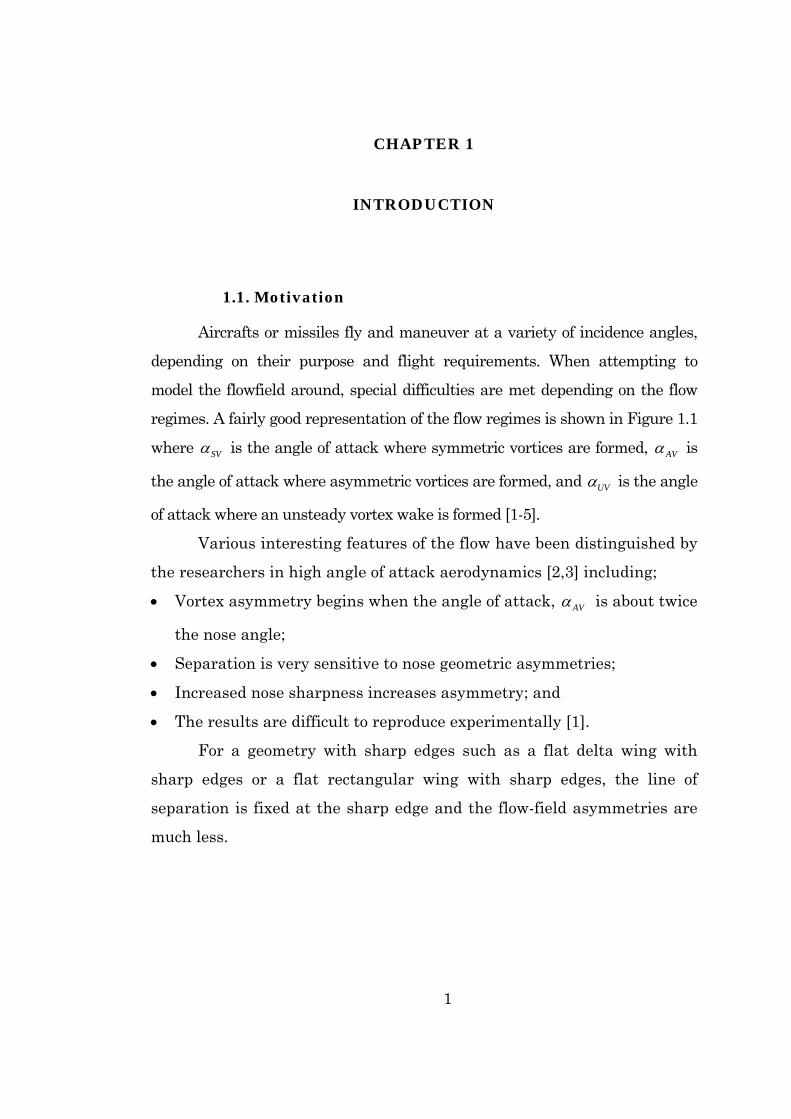
1.1. Motivation

Aircrafts or missiles fly and maneuver at a variety of incidence angles,

depending on their purpose and flight requirements. When attempting to

model the flowfield around, special difficulties are met depending on the flow

regimes. A fairly good representation of the flow regimes is shown in Figure 1.1

where SVα is the angle of attack where symmetric vortices are formed, AVα is

the angle of attack where asymmetric vortices are formed, and UVα is the angle

of attack where an unsteady vortex wake is formed [1-5].

Various interesting features of the flow have been distinguished by

the researchers in high angle of attack aerodynamics [2,3] including;

• Vortex asymmetry begins when the angle of attack, AVα is about twice

the nose angle;

• Separation is very sensitive to nose geometric asymmetries;

• Increased nose sharpness increases asymmetry; and

• The results are difficult to reproduce experimentally [1].

For a geometry with sharp edges such as a flat delta wing with

sharp edges or a flat rectangular wing with sharp edges, the line of

separation is fixed at the sharp edge and the flow-field asymmetries are

much less.

2

Figure 1.1 Angle of attack flow regimes [1-5].

Separated and complex turbulent flows have extensively been

studied by experiments and numerical simulations to yield distributions

of statistical flow properties such as time-mean velocities, pressure,

Reynolds stresses, correlations, and spatio-temporal structure of large-

scale vortices. Kiya, M. [6] states the following remarks; “These are

experimental results, which are useful in the design of flow apparatus,

but to have experimental results is not equivalent to understand the flow.

The advance of numerical simulations and experiments aided by high

technology such as lasers and computers is just to make it rapid and

economical to obtain the experimental results. A flow is understood when

a physical or mathematical model that can predict essential properties of

the flow is constructed. In this sense, we have not yet understood

separated flows. This is because unsteadiness due to the motion of large-

3

scale vortices and their three-dimensionality are characteristic of

separated flows”.

The main goal on this work is to test the validity of the Navier-

Stokes code on the prediction of separated flows, in particular, the ones

around the low aspect ratio wings.

1.2. General Features of the Separated Flows

Separated flows can be classified into two categories; the flow

without reattachment and the flow with reattachment [6]. The flow

without reattachment occurs around cylindrical bluff bodies such as

circular cylinders and normal plates and it is characterized by the

interaction between vortices, which is shed from the separation points.

However, the flow over a backward-facing step, blunt plates or blunt

circular cylinders are the typical examples of the flow with reattachment,

which is characterized by the interaction between vortices and the solid

surface and a separation bubble formation [6].

Separation can be described as the entire process in which a flow

detaches from a solid surface, resulting in a breakdown of the boundary

layer while undergoing a sudden thickening and causing an increased

interaction between the viscous-inviscid layers [7].

Alving & Fernholz [8] make a distinction between separation

caused by sharp gradients in the surface geometry, denoted geometry-

induced separation, and separation from smooth surfaces caused by

adverse pressure gradients -“adverse-pressure-gradient-induced

separation” – and discuss in general terms differences between these two

cases as seen on Figure 1.2.

4

Figure 1.2 Separation types

In terms of the leading edge bluntness, the sharp leading edge

produces less complex flow with respect to the blunt leading edge [9]. At

high Reynolds number, flow past a blunt body typically leads to the

formation of a turbulent separation bubble near the sharp corner as well

as the emergence of a reattaching flow further downstream [10,13]. The

separation bubble is characterized by rolled-up vortices in the shear layer

and their interaction with the surface [10-12,14]. The presence of a

separated flow, together with a reattaching flow, gives rise to

unsteadiness, pressure fluctuations and vibrations of the structure

through which the fluid is flowing [15].

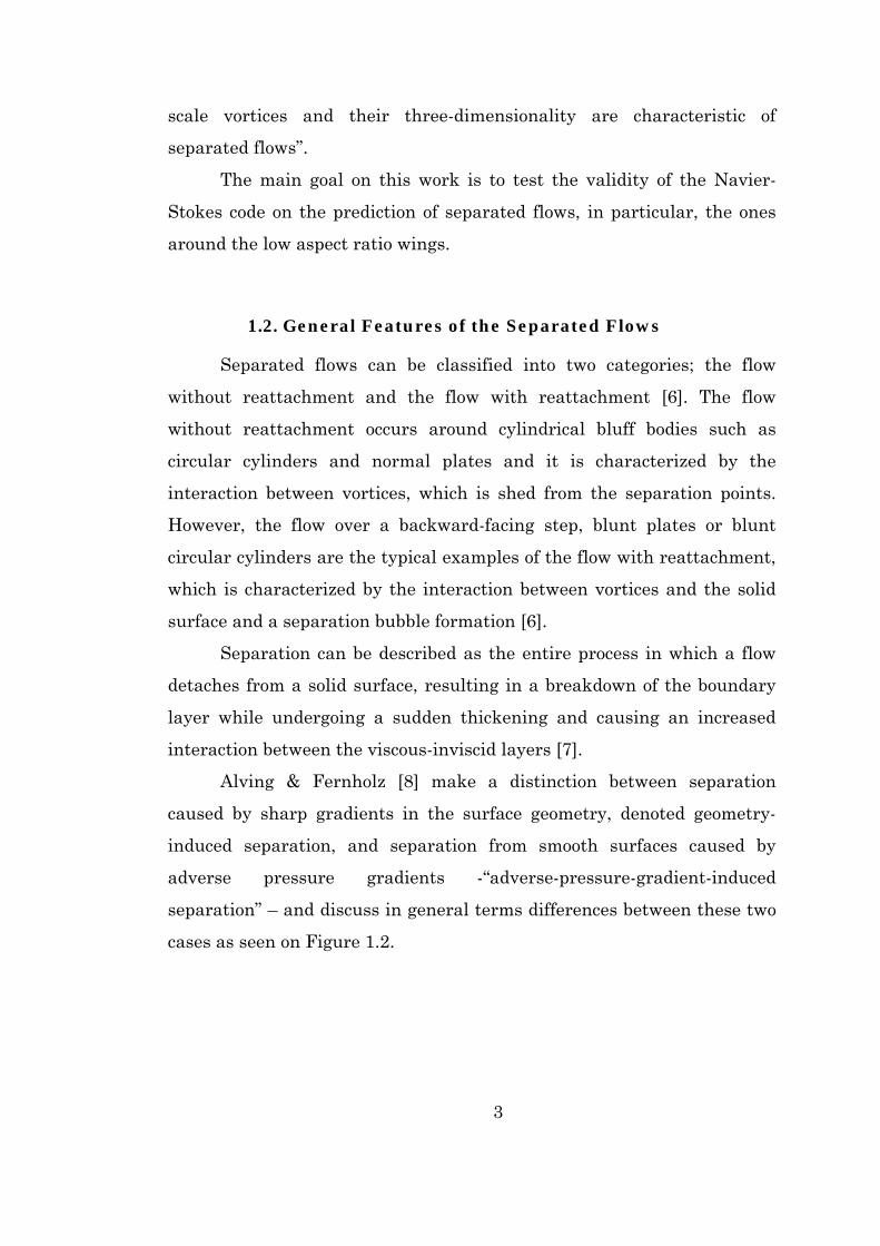
The pressure plateaus seen in Figure 1.3 indicate that the speed of

the fluid particles in separated flow regions is very slow. This observation

led to the common term “dead-air region” or “dead-water region”.

Although the static pressure remains almost constant further

downstream, the pressure recovers quickly as the aft portion of the time-

averaged separation bubble is approached. This corresponds to an intense

convection effect inside the bubble.

Separation bubble flow can also be classified as being laminar,

transitional or turbulent according to the separation and reattachment

status of the boundary layer [16]. In a laminar separation bubble, the

boundary layer is laminar at both separation and reattachment points,

while in the transitional bubble the boundary layer is still laminar at

separation but turbulent at reattachment. If the boundary layer is

5

turbulent at both separation and reattachment locations, the separation

bubble is called turbulent.

Figure 1.3 Separation bubble formation

Due to the unstable structure of the bubble, turbulent boundary

layer may be developed at lower Reynolds numbers, resulting in higher

drag. Separation bubbles have gained much attention due to its

computational character.

The forward&backward facing step geometries have been

extensively studied in much experimental and numerical work on

separated flows serve as cornerstone test cases. One reason for this is the

fact that the point of separation is fixed in space and time and that

separation occurs for all Reynolds numbers [16].

In the case of sharp leading edge bodies, the boundary layer

separates from the edge, being shed downstream as a separated shear

layer and as we increase the angle of attack, a fully separated flow

develops and the wing behaves as a bluff body [6]. Kiya, M. [6,17] states

that “spanwise vortices are formed by rolling up the shear layer through

the Kelvin-Helmholtz instability to form rectilinear vortex tubes whose

6

axis is aligned with the edge. The Spanwise vortices merge to become

larger and larger with increasing longitudinal distance from the edge. At

the same time the spanwise vortices deform in the spanwise direction,

being rapidly three-dimensionalized developing turbulence. Large-scale

vortices impinge on the surface of the body at a certain longitudinal

distance from the edge, being shed downstream. This position of

impingement is near the time-mean reattachment position of the shear

layer, which is defined as the longitudinal position at which the time-

mean streamline starting from the edge reattaches on the surface. The

pressure fluctuation generated by the impingement of the vortices

propagates upstream to be accepted at the sharp leading edge to generate

vorticity fluctuation, which enhances the rolling-up of the shear layer.

The resulting large-scale vortices subsequently impinge on the surface. In

this sense, the leading edge separation bubble is a self-excited flow

maintained by the feedback loop. The feedback mechanism is a working

hypothesis, having not been confirmed by experiments or numerical

simulations”. A description of the different feedback processes for blunt

bodies [18] is shown in Figure 1.4.

The number of merging of spanwise vortices up to the impingement

position, the length scale of the impinging vortices, and the frequency of

their shedding Fv are related to the height of the separated shear layer

from the surface [19]. In other words, it is related with the surface

pressure just downstream of the edge; the lower the surface pressure, the

higher is the curvature or height [6].

The Kelvin-Helmholtz instability and the Shedding-type or

Impinging-type of instability [6,19,20] are the two types of instability

within the separation bubble.

7

Figure 1.4 Schematic of feedback loops of locked vortex shedding for blunt leading-edge plates with either blunt or streamlined trailing edges [18].

The fundamental frequency of the Kelvin-Helmholtz instability

scales to the momentum thickness of the shear layer at the separation

edge and the velocity, thus being a function of Reynolds number. On the

other hand, the fundamental frequency of the shedding-type instability

also called vortex-shedding frequency is practically constant at sufficiently

high Reynolds numbers. Sigurdson [19] argues that the shedding-type

instability is the primary mode of instability in the separation bubble.

Low-frequency modulation is also observed in nominally two-

dimensional and axisymmetric separated-and-reattaching flows:

backward-facing step flows; leading-edge separation bubbles of blunt

plates and blunt circular cylinders. The modulation in these flows is

sometimes referred to as flapping because it is accompanied by a

transverse oscillation of the separated shear layer. The flapping motion is

an intrinsic property of the separation bubbles, not being due to

extraneous effects from end effects [6]. The experimental studies (e.g.,

Cherry et al. [10]; Kiya and Sasaki [11]; Djilali and Gartshore [21];

Saathoff and Melbourne [22]) around a bluff rectangular plates at high

8

Reynolds numbers report a characteristic low frequency flapping of the

separated shear layer as well as pseudo periodic vortex shedding from the

separation bubble [23].

Three-dimensional separations can also be classified in three

groups with respect to their topology and kinematics shown in Figure 1.5.

In Yates and Chapman [24], Horseshoe and Werle type separations are

defined as global separations (or closed separations). It is stated clearly in

reference [23] that “the predominant structures over the separation

bubble are clearly identified as hairpin (horseshoe) vortices in the

reattachment region. The legs of the horseshoe vortices are inclined with

respect to the streamwise direction. A typical vortex grows in every

direction as it is advected downstream of the reattachment region. Due to

the interaction between the vortical motion of the large-scale structure

and the wall, it also tends to lift away from the wall. This in turn, brings

the top end of the horseshoe vortex into contact with the outer (higher

velocity) region, resulting in further stretching and inclination of the

vortex along the flow direction. Eventually, the central portion breaks

down, and only the two inclined legs remain. This phenomenon takes

place in the recovery region. The unsteady motion from the shedding of

these large-scale vortices causes oscillations and meandering of the

instantaneous reattachment (zero-shear stress) line”.

A typical oscillation consists of two distinct phases: (i) gradual

growth of large-scale structures in the separated shear layer,

accompanied by a progressive growth of the separation bubble, (ii)

shedding of a large-scale structure followed by a collapse of the bubble

and abrupt shortening of the reattachment length [23].

9

Figure 1.5 Limiting streamline pattern and surfaces of separation for three types of 3-D separation. Taken from Yates and Chapman [24].

Figure 1.6. Singular points

Horseshoe type seperation

Werle type seperation

Cross flow separation

10

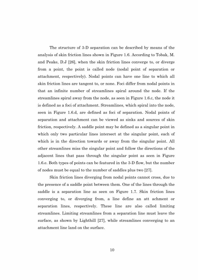
The structure of 3-D separation can be described by means of the

analysis of skin friction lines shown in Figure 1.6. According to Tobak, M.

and Peake, D.J [26], when the skin friction lines converge to, or diverge

from a point, the point is called node (nodal point of separation or

attachment, respectively). Nodal points can have one line to which all

skin friction lines are tangent to, or none. Foci differ from nodal points in

that an infinite number of streamlines spiral around the node. If the

streamlines spiral away from the node, as seen in Figure 1.6.c, the node it

is defined as a foci of attachment. Streamlines, which spiral into the node,

seen in Figure 1.6.d, are defined as foci of separation. Nodal points of

separation and attachment can be viewed as sinks and sources of skin

friction, respectively. A saddle point may be defined as a singular point in

which only two particular lines intersect at the singular point, each of

which is in the direction towards or away from the singular point. All

other streamlines miss the singular point and follow the directions of the

adjacent lines that pass through the singular point as seen in Figure

1.6.e. Both types of points can be featured in the 3-D flow, but the number

of nodes must be equal to the number of saddles plus two [27].

Skin friction lines diverging from nodal points cannot cross, due to

the presence of a saddle point between them. One of the lines through the

saddle is a separation line as seen on Figure 1.7. Skin friction lines

converging to, or diverging from, a line define an att achment or

separation lines, respectively. These line are also called limiting

streamlines. Limiting streamlines from a separation line must leave the

surface, as shown by Lighthill [27], while streamlines converging to an

attachment line land on the surface.

11

Figure 1.7. Line of separation

Nodal points of separation and attachment are other interesting

features: they become edges of vortex cores. In some cases, there is also a

distinction between primary and secondary lines of separation. Most

researchers agree that the convergence of streamlines on either side of a

particular line is a necessary condition for separation however; it should

not be used solely to define it as this may occur in other situations as

well.

1.3. General Description of the Flowfield around the Low Aspect Ratio Wings

The flowfield around the low aspect ratio wings are mainly

characterized by the separations at the leading edge and at the side edges

of the wing. The separation at the leading edge leads to separation bubble

whereas the separation at the side edges results in tip vortices. There is a

strong interference between separation bubble and side vortices at high

incidences. This makes the flowfield around these wings quite

complicated [28].

At even lower aspect ratios, the wing is subject to strong vortex

flows and CL increases at a faster rate than that predicted with a linear

theory [29]. This is due to the presence of the strong tip vortices that

separate closer to the leading edge, according to a mechanism similar to

12

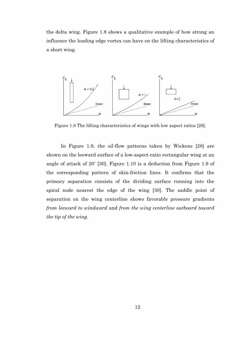
the delta wing. Figure 1.8 shows a qualitative example of how strong an

influence the leading edge vortex can have on the lifting characteristics of

a short wing.

Figure 1.8 The lifting characteristics of wings with low aspect ratios [29].

In Figure 1.9, the oil-flow patterns taken by Wickens [28] are

shown on the leeward surface of a low-aspect-ratio rectangular wing at an

angle of attack of 20° [30]. Figure 1.10 is a deduction from Figure 1.9 of

the corresponding pattern of skin-friction lines. It confirms that the

primary separation consists of the dividing surface running into the

spiral node nearest the edge of the wing [30]. The saddle point of

separation on the wing centerline shows favorable pressure gradients

from leeward to windward and from the wing centerline outboard toward

the tip of the wing.

13

Figure 1.9 Oil-flow pattern on slender, rectangular wing, aspect ratio 0.25 at 20α = ° [28]

Figure 1.10 Interpretation of skin-friction lines and pressures on slender, rectangular wing, aspect ratio 0.25 at 20α = ° [28].

14

The low aspect ratio rectangular flat wings especially with sharp

leading and side edge generally have the flowfield shown in Figure 1.11.

Flow separates at the sharp leading edge and forms the leading edge

bubble. There are two side, or tip vortices called as spanwise vortices. In

the side edges, there exist also secondary vortices and reversed flows also

shown in Figure 1.12. Moreover, a secondary bubble underneath the

primary bubble is formed as illustrated in Figure 1.13. The rolling up

vortices or hairshoe vortices within the separation bubble and the

spanwise vortices interact with each other causing a more complex

flowfield, which has unsteady, oscillating structure.

Figure 1.11 Illustrative 3-d flowfield around the low-aspect ratio flat wings.

U∞ α

15

Figure 1.12 Illustrative flowfield at the symmetry plane.

Figure 1.13 Illustrative flowfield at the spanwise plane.

16

1.4. Literature Review on Low Aspect Ratio Wings

In the past twenty years, great advances in technology have led to

significant advances in fluid mechanics. Various publications by AGARD

[28,32-35] provide a large selection of research results in this field. Low

aspect ratio rectangular flat wings, however were studied much less when

compared to the Delta wings of the similar nature. Stahl [36] summarized

some of the early research works. Winter [37] obtained pressure

distributions on the suction side and force and moment measurements of

various low aspect ratio rectangular flat wings at incompressible speeds.

At von Karman Institute, similar experiments [38,39] were performed in

a transonic wind tunnel for higher speeds.

Simpson [25,41,42] has periodically reviewed the topic of separated

flow over the years providing a history of the understanding of turbulent

flow separation [40]. A detailed investigation into the literature of the

separated and reattaching flow is found by Cherry at al. [10]. A

comprehensive review of the global instability was associated with these

sorts of flows by Rockwell [43].

Extraction of large-scale vortical structure from turbulent

separated and reattaching flows have been studied by numerous studies

using conditional averaging techniques [10,12,44]. A strong negative

correlation was captured caused by the low-frequency flapping motion of

the vortex shedding used a surface pressure sensor to educe the structure

of large-scale vortices [12]. Kiya and Sasaki [12] was identified a saw-

tooth like movement of the separation bubble and hairpin vortices in

their conditional average. The existence of a large-scale vortex was also

indicated by revealing that the location of maximum vorticity coincides

with that of maximum turbulence intensity [12,46]. The characteristic

frequencies and intermittent nature of the pseudo periodic vortex

17

shedding from the separated shear layer and the reattachment region, as

well as the shear layer flapping were captured in the large-eddy

simulation of separated flow over a bluff rectangular plate [23].

Analyses of the leading-edge separation have been performed by

many experiments and computations [47,48]. Recent experiment at NASA

Langley Research Center investigated effects of leading-edge bluntness

and Reynolds-number difference [49,50]. Numerical simulation around

delta wing with sharp and blunt leading edges has been performed to

investigate the leading edge bluntness and Reynolds-number effects

suggested by the experiment [9].

The flow around rectangular plates in the absence of any external

forcing has been studied previously both experimentally and numerically

[20]. A series of simulations of flows around blunt rectangular plates have

been under taken to test the hypothesis that the trailing edge shedding

plays an important role in the mechanism leading to self sustained

oscillations [6]. The same mechanism may in fact be the feedback loop

generated by the impinging leading edge vortices in the absence of

trailing edge vortex shedding [43].

The mean flow characteristics and large-scale unsteadiness aspects

of turbulent flow around a bluff rectangular plate have been the subject of

a number of experimental studies at high Reynolds numbers [10,11,21].

All studies report a characteristic low frequency flapping of the separated

shear layer as well as pseudo periodic vortex shedding from the

separation bubble [23].

An adequate representation of the mean flow characteristics within

the separation bubble have been provided by Reynolds-averaged Navier-

Stokes (RANS) Solution of the high Reynolds number turbulent flow [20].

Impinging shear layer instability was initially classified by

Nakamura & Nakashima [20]and Nakamura et al. [52]. Later studies

[53-57] preferred the description impinging leading edge vortex

18

instability because it better describes the process wherein leading-edge

vortices are shed, convected downstream and then interact with the

trailing edges.

The instability waves in the diverging shear flow over square and

circular plates were studied in a water tank using flow visualization

techniques at angles of attack between 6o and 18o and it was found that

small-large scale instability waves were generated in the shear layer over

a flat plate at incidence [58].

Alving & Fernholz [59] distinguish between “strong” and “mild”

separation bubbles based on the height of the shear layer upstream of

separation relative to the height of the separation bubble. A separation

bubble is referred to as a “strong” bubble when the height of the shear

layer preceding separation is of the same size or smaller than the height

of the bubble, whereas, conversely, in a “mild” separation bubble the

height of the bubble is considerable smaller than the pre-separated shear

layer.

A variety of influences on high angle of attack flow predictions

have been discussed, including: governing equation complexity,

turbulence modeling, transition modeling, algorithm symmetry, grid

generation and density, and numerical dissipation [1]. Non-linear inviscid

methods which account for the leading edge vortices and their

interactions with the wing surfaces have been developed and modeled the

behavior of high Reynolds number , turbulence flow over sharp- edged

wings extremely well [60].

Computational procedures allowing aerodynamicists to investigate

flows using complex three-dimensional computational fluid dynamics

(CFD) to extract the flow topology are now widely available [61]. Delery

[62] states that Legendre [63] pioneered flow topology research by

proposing that wall streamlines be considered as trajectories having

properties consistent with those of a continuous vector field, the principal

19

being that through any nonsingular point there must pass one and only

one trajectory. Different combinations of nodal/saddle points and how

they work together have received much attention by Tobak and Peake

[26] and Chapman [64]. Since then, much research has been done on fluid

flow topology, ranging from Chapman [64] and Wang [65] who classified

flow topology for separation on three-dimensional bodies to Cipolla and

Rockwell [66] who investigated the instantaneous crossflow topology

using particle image velocimetry. Hunt et al. [67] have shown that the

notions of singular points and the rules that they obey can be extended to

apply to the flow above the surface on planes of symmetry and on

crossflow planes. The classification of three-dimensional singular points

for flow topology has enabled aerodynamicists to successfully investigate,

predict, and fix the separation phenomena alleviating adverse

aerodynamic characteristics associated with separation.

1.5. Outline of Dissertation

After introducing the scope of our dissertation, Navier-Stokes

equations are presented in detail in Chapter 1. The following chapter

focuses on the solution algorithm used. In Chapter 4, the development of

hyperbolic grid generation code with upwind differencing is discussed.

The turbulence models adapted in the solution are examined in Chapter

5. The Test Cases and Results, which is the section where the most of the

work are performed, are presented in Chapter 6. In this chapter, test

cases are examined in two main sections. First, two-dimensional test

cases are studied within two sub sections; “Laminar Flat Plate” and

“Turbulent Flat Plate”. Then, three-dimensional test case; “Three

Dimensional Flat Plate”, which is the main goal of the thesis, is

presented. Results of each test case are discussed in the corresponding

section. In the last chapter, the conclusion and the future work are

presented.

20

CHAPTER 2

NAVIER STOKES EQUATIONS

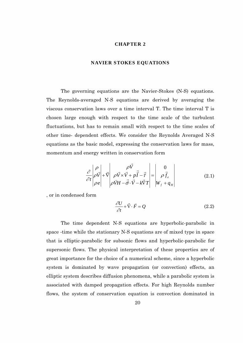
The governing equations are the Navier-Stokes (N-S) equations.

The Reynolds-averaged N-S equations are derived by averaging the

viscous conservation laws over a time interval T. The time interval T is

chosen large enough with respect to the time scale of the turbulent

fluctuations, but has to remain small with respect to the time scales of

other time- dependent effects. We consider the Reynolds Averaged N-S

equations as the basic model, expressing the conservation laws for mass,

momentum and energy written in conservation form

Hf

e

qWf

TkVHVIpVV

V

eV

t+

=∇−⋅−−+×∇+ ρ

σρτρ

ρ

ρρρ

∂∂

0 (2.1)

, or in condensed form

∂∂Ut

F Q+∇⋅ = (2.2)

The time dependent N-S equations are hyperbolic-parabolic in

space -time while the stationary N-S equations are of mixed type in space

that is elliptic-parabolic for subsonic flows and hyperbolic-parabolic for

supersonic flows. The physical interpretation of these properties are of

great importance for the choice of a numerical scheme, since a hyperbolic

system is dominated by wave propagation (or convection) effects, an

elliptic system describes diffusion phenomena, while a parabolic system is

associated with damped propagation effects. For high Reynolds number

flows, the system of conservation equation is convection dominated in

21

most of the flow region. The N-S equations are often written in vector

form as in Equation (2.2). For convenience, the equations are cast in

Cartesian coordinate form.

⎟⎟⎠

⎞⎜⎜⎝

⎛++=++++

zG

yF

xEH

zG

yF

xE

tq vvv

∂∂

∂∂

∂∂

∂∂

∂∂

∂∂

∂∂

Re1

(2.3)

These five equations are statements of the conservation of mass and

energy and conservation of momentum in the x, y and z directions. This

form of the equations assumes that the fluid may be compressible and

that heat generation and body forces (except for those, which might be

included in the source term, H ) can be ignored. This vector equation

states that the time rate of change in the dependent variables q is equal

to the spatial change in the inviscid fluxes, E, F and G, and viscous

fluxes, Ev , Fv and Gv . A source term, H, is included to account for the

centrifugal and Coriolis force terms, which appear if the coordinate frame

is rotating. In the present study, the source term was not taken into

account. The presence of the Reynolds number, Re u L= ρ µ , implies that

the governing equations have been non-dimensionalized; with ρ and u

often chosen as the freestream density and velocity, L chosen as the

reference length of the body and µ evaluated at the freestream static

temperature. The vector of dependent variables, the inviscid and viscous

flux terms are shown below.

( ) ( )

2

2

u vu p u vu

u v v pq E Fvu w v ww

e p u e p ve

ρ ρρρ ρρρ ρρρ ρρ

⎡ ⎤ ⎡ ⎤⎡ ⎤⎢ ⎥ ⎢ ⎥⎢ ⎥ +⎢ ⎥ ⎢ ⎥⎢ ⎥⎢ ⎥ ⎢ ⎥+⎢ ⎥= = =⎢ ⎥ ⎢ ⎥⎢ ⎥⎢ ⎥ ⎢ ⎥⎢ ⎥⎢ ⎥ ⎢ ⎥⎢ ⎥ + +⎣ ⎦ ⎣ ⎦ ⎣ ⎦

22

( )

2

0

xx

xyv

xz

xx xy xz x

wu wv wG E

w pu v w qe p w

ρτρτρτρ

τ τ τ

⎡ ⎤⎡ ⎤⎢ ⎥⎢ ⎥⎢ ⎥⎢ ⎥⎢ ⎥⎢ ⎥= =⎢ ⎥⎢ ⎥+ ⎢ ⎥⎢ ⎥⎢ ⎥⎢ ⎥ + + −+⎣ ⎦ ⎣ ⎦

0 0

yx zx

yy zyv v

yz zz

yx yy yz y zx zy zz z

F G

u v w q u v w q

τ ττ ττ τ

τ τ τ τ τ τ

⎡ ⎤ ⎡ ⎤⎢ ⎥ ⎢ ⎥⎢ ⎥ ⎢ ⎥⎢ ⎥ ⎢ ⎥= =⎢ ⎥ ⎢ ⎥⎢ ⎥ ⎢ ⎥⎢ ⎥ ⎢ ⎥+ + − + + −⎣ ⎦ ⎣ ⎦

Here ρ is the fluid density; u , v and w are the fluid velocities in

the x, y and z coordinate directions, and e is the total energy per unit

volume. The viscous flux terms are functions of the local fluid velocities,

the shear stresses, τxx , and heat conduction terms qx , qy and qz .

The pressure, p , which appears in the inviscid flux terms, is

related to the dependent variables through an appropriate equation of

state. The local pressure is expressed in terms of the dependent variables

by applying the ideal gas law.

( ) ( )[ ]222211 wvuep ++−−= ργ (2.4)

The stresses are related to the velocity gradient of the fluid,

assuming a Newtonian fluid for which the viscous stress is proportional

to the rate of shearing strain (i.e. angular deformation rate). For

turbulent flow, a Reynolds-averaged form of the equations is used where

the dependent variables represent the mean flow contribution. The

Boussinesq assumption is applied, permitting the apparent turbulent

stresses to be related to the product of the mean flow strain rate and an

apparent turbulent viscosity. Therefore, the shear and normal stress

tensors have the following form;

23

( )

( )

23

23

ji kij ij T ij

j i k

ji kij T ij

j i k

uu upx x x

uu ux x x

∂∂ ∂σ δ µ µ δ∂ ∂ ∂

∂∂ ∂τ µ µ δ∂ ∂ ∂

⎡ ⎤⎛ ⎞= − + + + −⎢ ⎥⎜ ⎟⎜ ⎟⎢ ⎥⎝ ⎠⎣ ⎦

⎡ ⎤⎛ ⎞= + + −⎢ ⎥⎜ ⎟⎜ ⎟⎢ ⎥⎝ ⎠⎣ ⎦

(2.5)

The heat conduction terms, when Reynolds-averaging and the

Boussinesq assumption are applied, are proportional to the local mean

flow temperature gradient;

( ) ( )2

11i T

i

Tq k kPrM x

∂γ ∂∞

−= +

− (2.6)

Here, γ represents the ratio of specific heats, Pr is the Prandtl

number and M∞ is the freestream Mach number.

To determine the effective turbulent conductivity, Tk , Reynolds

analogy is applied and the turbulent conductivity is related to the

turbulent viscosity as follows;

T TT

PrkPr

µ= (2.7)

Here, and in the equation above, the conductivity and viscosity are

non-dimensionalized by their representative (laminar) values evaluated

at the freestream static temperature.

In many CFD applications, it is desirable to solve the governing

equations in a domain, which has surfaces that conform to the body

rather than in a Cartesian coordinate domain. A transformation is

applied to the original set of equations to obtain a "generalized geometry"

form of the governing equations. This allows the irregular shaped

physical domain to be transformed into a rectangular shaped

computational domain that allows the numeric to be simplified

somewhat. This transformation also simplifies the applications of the

boundary conditions and may include various options on grid point

24

clustering and orthogonality, both being extremely important for the

solution of the Navier-Stokes equations. Obviously, grid point clustering

near the surface for viscous flows is required in order to resolve the flow

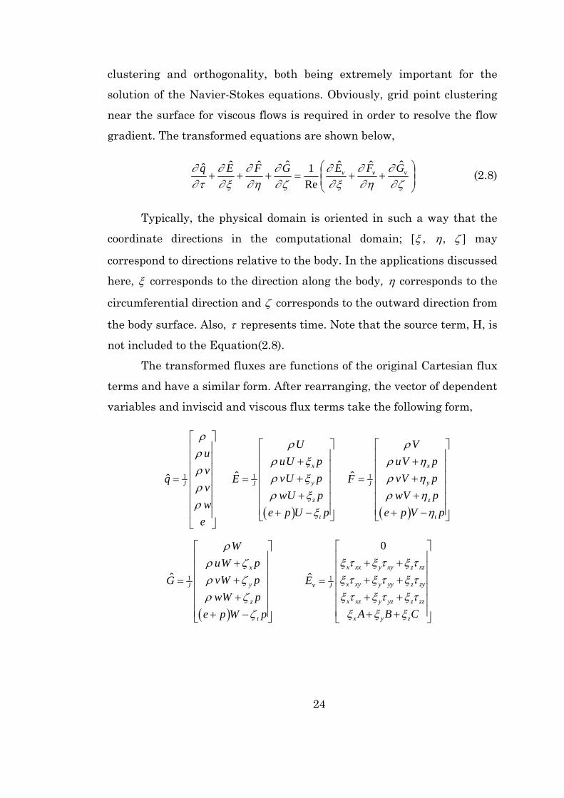
gradient. The transformed equations are shown below,

⎟⎟⎠

⎞⎜⎜⎝

⎛++=+++

ζ∂∂

η∂∂

ξ∂∂

ζ∂∂

η∂∂

ξ∂∂

τ∂∂ vvv GFEGFEq ˆˆˆ

Re1ˆˆˆˆ (2.8)

Typically, the physical domain is oriented in such a way that the

coordinate directions in the computational domain; [ξ , η, ζ ] may

correspond to directions relative to the body. In the applications discussed

here, ξ corresponds to the direction along the body, η corresponds to the

circumferential direction and ζ corresponds to the outward direction from

the body surface. Also, τ represents time. Note that the source term, H, is

not included to the Equation(2.8).

The transformed fluxes are functions of the original Cartesian flux

terms and have a similar form. After rearranging, the vector of dependent

variables and inviscid and viscous flux terms take the following form,

( ) ( )

1 1 1ˆ ˆˆ x x

y yJ J J

z z

t t

U Vu

uU p uV pv

vU p vV pq E Fv

wU p wV pw

e p U p e p V pe

ρρ ρ

ρρ ξ ρ η

ρρ ξ ρ η

ρρ ξ ρ η

ρξ η

⎡ ⎤⎡ ⎤ ⎡ ⎤⎢ ⎥⎢ ⎥ ⎢ ⎥⎢ ⎥ + +⎢ ⎥ ⎢ ⎥⎢ ⎥⎢ ⎥ ⎢ ⎥+ += = =⎢ ⎥⎢ ⎥ ⎢ ⎥⎢ ⎥ + +⎢ ⎥ ⎢ ⎥⎢ ⎥⎢ ⎥ ⎢ ⎥+ − + −⎢ ⎥ ⎣ ⎦ ⎣ ⎦

⎣ ⎦

( )

1 1

0

ˆ ˆ x xx y xy z xzx

x xy y yy z zyy vJ J

x xz y yz z zzz

x y zt

WuW pvW pG EwW p

A B Ce p W p

ρξ τ ξ τ ξ τρ ζξ τ ξ τ ξ τρ ζξ τ ξ τ ξ τρ ζξ ξ ξζ

⎡ ⎤⎡ ⎤⎢ ⎥⎢ ⎥ + ++ ⎢ ⎥⎢ ⎥⎢ ⎥⎢ ⎥ + ++= =⎢ ⎥⎢ ⎥ + ++ ⎢ ⎥⎢ ⎥⎢ ⎥⎢ ⎥ + ++ −⎣ ⎦ ⎣ ⎦

25

1 1

0 0

ˆˆ x xx y xy z xz x xx y xy z xz

x xy y yy z zy x xy y yy z zyv vJ J

x xz y yz z zz x xz y yz z zz

x y z x y z

F G

A B C A B C

η τ η τ η τ ζ τ ζ τ ζ τη τ η τ η τ ζ τ ζ τ ζ τη τ η τ η τ ζ τ ζ τ ζ τη η η ζ ζ ζ

⎡ ⎤ ⎡ ⎤⎢ ⎥ ⎢ ⎥+ + + +⎢ ⎥ ⎢ ⎥⎢ ⎥ ⎢ ⎥+ + + += =⎢ ⎥ ⎢ ⎥+ + + +⎢ ⎥ ⎢ ⎥⎢ ⎥ ⎢ ⎥+ + + +⎣ ⎦ ⎣ ⎦

(2.9)

where

zzzzyzx

yyzyyyx

xxzxyxx

qwvuCqwvuB

qwvuA

−++=

−++=

−++=

τττ

τττ

τττ

The velocities in the , ξ η and ζ coordinates represent the

contravariant velocity components.

t x y z

t x y z

t x y z

U u v w

V u v w

W u v w

ξ ξ ξ ξ

η η η η

ζ ζ ζ ζ

= + + +

= + + +

= + + +

(2.10)

The Cartesian velocity components (U, V, W) are retained as the

dependent variables and are non-dimensionalized with respect to a∞ (the

freestream speed of sound). In addition to the original Cartesian

variables, additional terms ( ),...,,, zyxJ ζηξ appear in the equations. These

terms referred to as the metric terms, result from the transformation and

contain the purely geometric information that relates the physical space

to the computational space. The metric terms are defined as

( ) ( ) ( )( ) ( ) ( )( ) ( ) ( )

x x x

y y y

z z z

J y z y z J z y y z J y z z y

J z x x z J x z x z J z x x z

J x y y x J y x x y J x y y x

η ζ ζ η ξ ζ ξ ζ ξ η ξ η

η ζ η ζ ξ ζ ζ ξ ξ η ξ η

η ζ η ζ ξ ζ ξ ζ ξ η ξ η

ξ η ζ

ξ η ζ

ξ η ζ

= − = − = −

= − = − = −

= − = − = −

(2.11)

and

26

( )( )

1 , ,, ,

x y zJ x y z x y z x y z x y z x y z x y zξ η ζ ζ ξ η η ζ ξ ξ ζ η η ξ ζ ζ η ξ

∂∂ ξ η ζ

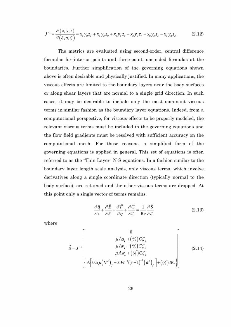
− = = + + − − − (2.12)

The metrics are evaluated using second-order, central difference

formulas for interior points and three-point, one-sided formulas at the

boundaries. Further simplification of the governing equations shown

above is often desirable and physically justified. In many applications, the

viscous effects are limited to the boundary layers near the body surfaces

or along shear layers that are normal to a single grid direction. In such

cases, it may be desirable to include only the most dominant viscous

terms in similar fashion as the boundary layer equations. Indeed, from a

computational perspective, for viscous effects to be properly modeled, the

relevant viscous terms must be included in the governing equations and

the flow field gradients must be resolved with sufficient accuracy on the

computational mesh. For these reasons, a simplified form of the

governing equations is applied in general. This set of equations is often

referred to as the "Thin Layer" N-S equations. In a fashion similar to the

boundary layer length scale analysis, only viscous terms, which involve

derivatives along a single coordinate direction (typically normal to the

body surface), are retained and the other viscous terms are dropped. At

this point only a single vector of terms remains.

ζ∂

∂ζ∂

∂η∂

∂ξ∂

∂τ∂

∂ SGFEq ˆ

Re1ˆˆˆˆ

=+++ (2.13)

where

( )( )( )

( ) ( ) ( ) ( )

3

1 3

3

12 1 23

0

ˆ

0.5 V 1

x

y

z

Au CAv CS JAw C

A Pr a BC

µζ

µζ

µζ

µζ ζ

µ ζµ ζµ ζ

µ κ γ

−

−−

⎡ ⎤⎢ ⎥+⎢ ⎥⎢ ⎥+= ⎢ ⎥+⎢ ⎥⎢ ⎥⎡ ⎤+ − +⎢ ⎥⎣ ⎦⎣ ⎦

(2.14)

27

with

2 2 2 2 2 2 2

2

V

1

x y z

x y z

x y z

A u v w

B u v wRM

C u v wζ ζ ζ

ζ ζ ζ

ζ ζ ζ κγ

ζ ζ ζ∞

= + + = + +

= + + =

= + +

With this form of equations, the cross-derivatives in the viscous

terms have been eliminated. The equations are now in a form, which is

amenable to solution by direct implicit numerical techniques such as the

Beam and Warming algorithm.

28

CHAPTER 3

SOLUTION ALGORITHM

The numerical scheme used for the solution of the Thin Layer N-S

equations is generally based on a fully implicit, approximately factored,

finite difference algorithm in delta form [82]. Implicit methods with the

delta form are widely used for solving steady state problems since the

steady state solutions are indifferent to the left-hand side operators.

The solution of the three-dimensional equations is implemented by

an approximate factorization that allows the system of equations to be

solved in three coupled one-dimensional steps. The most commonly used

method is the Beam and Warming one [83]. The LU-ADI factorization

[84]is one of those schemes that simplify inversion works for the left-hand

side operators of the Beam and Warming's. Each ADI operator is

decomposed to the product of the lower and upper bi-diagonal matrices by

using the flux vector splitting technique [84].

To maintain the stability, the diagonally dominant LU

factorization is adopted. The explicit part is left to be the same as the

Beam and Warming's where central differencing is used. .

As indicated in Equation (2.13) , this solution technique involves

solving the time-dependent N-S equations. The procedure is started by

assuming a uniform, free-stream solution for all grid points in the

computational domain. The calculation then marches in time until a

steady state solution is obtained subject to the imposed boundary

conditions.

Beam and Warming method applied to Equation (2.13) leads to the

following approximate factorization form,

29

( ) ( )( ) ( )

( )

1 1

1 1 1

1 1 2 2 2

ˆ ˆ

ˆ ˆ ˆˆRe

ˆ ˆˆ ˆ Re ( ) ( ) ( )

n ni i

n n n ni

n n n n ne

I h A J J I h B J J

I h C h M J J Q Q

h E F G S J JQ

ξ ξ ξ η η η

ζ ζ ζ ζ

ξ η ζ ζ ξ ξ η η ζ ζ

δ δ

δ δ

δ δ δ δ

− −

− − +

− −

+ −∈ ∇ ∆ × + −∈ ∇ ∆ ×

+ − −∈ ∇ ∆ × −

⎡ ⎤= − + + − −∈ ∇ ∆ + ∇ ∆ + ∇ ∆⎣ ⎦

(3.1)

where h t= ∆ , δ is the central finite difference operator, and ∆and

∇ are forward and backward difference operators, respectively.

For the convective terms in the right hand side, fourth order

differencing is used. Maintenance of the freestream is achieved by

subtracting the freestream fluxes from the governing equations.

For the ξ direction, the Beam and Warming's ADI operator can be

written in the diagonal form as follows,

1 2 1 2 1ˆ ˆi A iI h A J J T I h D J J Tξ ξ ξ ξ ξ ξδ δ δ δ− − −⎡ ⎤+ + ∈ = + + ∈⎣ ⎦ (3.2)

where 1ˆ ˆ

AA T D Tξ ξ−= .

The flux vector splitting technique is used to decompose the central

differencing to two one sided differencing.

1ˆA AA T I D D Tξ ξ ξ ξ+ − −⎡ ⎤= +∇ + ∆⎣ ⎦ (3.3)

with

( ) JJDDD iAAh

A ∈±±= −± 12

ˆˆ (3.4)

where J −1 is taken to be the Jacobian at the central point

corresponding to Equation (3.2). Equation (3.3) can be rewritten as,

[ ] 1ˆA A AA T L M N Tξ ξ

−= + + (3.5)

where for three point upwinding,

30

L D DA A Aj j= − ++ +

− −86

161 2

,

( )jj AAA DDIM −+ −+= 67 ,

N D DA A Aj j= −− −

+ +86

161 2

,

The diagonally dominant factorization used here can be described

as,

( ) ( ) ( )1 20A A A A A A A AL M N L M M M N h−+ + = + + + (3.6)

since ( )0 1AM = and LA, N hA = 0( ).

Thus, the LU factorization for an ADI operator can be obtained as

JJAhI i21ˆξξ δδ ∈++ − ( ) ( ) 11 −− ++= ξξ TNMMMLT AAAAA (3.7)

By this, the block tri-diagonal system is decomposed to the product

of the lower and upper scalar bi-diagonal ones, L MA A+ and

( )AAA NMM +−1 .

In order to maintain the stability of the thin layer viscous terms,

the splitted Jacobian matrices C± are modified as follows,

( ) 1ˆˆ −±± ±= ζζ ν TIDTC Cv (3.8)

where

ν µ ρ ζζ= 2 2r Re ∆ (3.9)

At the end, the Beam and Warming Scheme can be described as follows

by using the similar procedure for the other operators,

( ) ( ) ( ) ( ) ( )

( ) ( ) ( )

1 1 1

1 1 1 ˆA A A A A B B B B B

nC C C C C

T L M M M N T T L M M M N

T T L M M M N T U RHS

ξ ξ η

η ζ ζ

− − −

− − −

× + × × + × × + × × + ×

× + × × + × ×∆ =

of (3.1).

31

As far as accuracy is concerned, the basic algorithm is first order

accurate in time and second order accurate in space. Convergence,

stability and smoothness of the solution depend on the implicit and

explicit smoothing factors, ∈i and ∈e and Courant-Friedrich-Lewy (CFL)

number. Physically, the CFL number indicates the relation between one

spatial step-size ∆x movement in one time step ∆t . Numerically, CFL

number is defined as:

( )ζηξσ

∆∆∆⋅∆

=,,min

maxtCFL (3.10)

Here σmax is the maximum eigenvalue. Starting from the definition

of speed of sound, σmax is defined as follows

( )CBA σσσσ ,,maxmax = (3.11)

where

( )2 2 22 1 2

p e u v wc γ γ γρ ρ⎛ ⎞+ += = − −⎜ ⎟⎝ ⎠

and

222

222

222

zyxC

zyxB

zyxA

cW

cV

cU

ζζζσ

ηηησ

ξξξσ

+++=

+++=

+++=

U, V and W were defined in Equation (2.10).

In order to simulate turbulence effects, the viscous coefficient is

computed as the sum of laminar viscosity and turbulence viscosity. The

turbulent eddy viscosity is then calculated by using the two-layer

algebraic turbulence model proposed by Baldwin and Lomax.

32

CHAPTER 4

HYPERBOLIC GRID GENERATION WITH UPWIND

DIFFERENCING

Hyperbolic grid generation provides efficiency, orthogonality and

superior control of the grid spacing. A conventional hyperbolic grid

generation method employs a central difference scheme and second- and

fourth-order dissipation terms are explicitly added for preventing

oscillation. These dissipation terms include user-specified constants.

Therefore, the decision of the constants strongly depends on the user's

experience. When the added dissipation is large, the grid-orthogonality

will be spoiled. On the contrary, when the dissipation is small the grid

smoothness will not be achieved and in the worst case, grid-line crossing

will occur.

An upwind difference scheme can be applied to the hyperbolic grid

generation since the system of the hyperbolic partial differential

equations has real distinct eigenvalues. Tai et al. [70] has applied the

Roe's flux-difference scheme to the hyperbolic grid generation, and

demonstrates excellent results employing first-order accurate upwind

scheme. The upwind scheme does not require the user-specified

parameters in general.

4.1. Governing Equations

The goal is to create a volume or surface grid by propagating grid

points from a given surface grid along a specified trajectory. The grid

point propagation is constrained by the equations defining the direction of

propagation (orthogonality) and the grid point spacing in the marching

33

direction. These constraint equations are found to be hyperbolic, making

a marching solution possible

A three dimensional grid point is defined as [ ]Tzyxr ,,≡ . The

computational coordinate system is defined using the three coordinates ξ,

η and ζ. The computational indices corresponding to the computational

coordinates are i, j and k respectively.

Generalized coordinates ξ(x,y,z), η(x,y,z), ζ(x,y,z) are sought where

the body surface is chosen to coincide with ζ(x,y,z)=0 and surface

distributions of ξ=constant and η=constant are user specified [68].

The governing equations are derived from orthogonality relations

between ξ and ζ, between η and ζ, and a cell volume constraint. Actually,

the constraint equations specify that the grid lines are to propagate from

the initial grid along a given trajectory and that the grid cell size is to

grow accordingly to a given function.

Hence, the mathematical development is based on three

constraints to allow a marching solution in the ζ direction for the three

unknowns x, y and z. The first two constraint imposes orthogonality of

grid lines at the surface as well as the interior domain. The third

constraint specifies the finite Jacobian, J [69].

The grid line trajectory in the marching direction is defined by two

angle (orthogonality) constraints:

. 0 r rξ ζ = (4.1)

and

. 0 r rη ζ = (4.2)

The third constraint is actually a specification of cell volume

according to

1( )r r r J Vξ η ζ−⋅ × = = (4.3)

34

Alternatively, in an expanded form, we can get the following

system of equations

. 0

. 0

( ) ( )

r r x x y y z zr r x x y y z z

r r r x y z x y z x y z x y z x y z x y z V

ξ ζ ξ ζ ξ ζ ξ ζ

η ζ η ζ η ζ η ζ

ξ η ζ ξ η ζ η ζ ξ ζ ξ η ξ ζ η η ξ ζ ζ η ξ

= + + =

= + + =

⋅ × = + + − + + =

(4.4)

Since the constraint equations form a system of nonlinear partial

differential equations, the system must be linearized about a known state

0r .in order to facilitate their numerical solution [69].

We define

0

0

0

x x xy y yz z z

= + ∆= + ∆= + ∆

(4.5)

, or

rrr ∆+= 0 (4.6)

After some manipulations, we get the linearized system in

conventional form,

0 0 0A r B r C r fξ η ζ+ + = (4.7)

and the coefficient matrices in the above equation.

35

⎪⎭

⎪⎬

⎫

⎪⎩

⎪⎨

⎧

+=

⎥⎥⎥

⎦

⎤

⎢⎢⎢

⎣

⎡

−−−=

⎥⎥⎥

⎦

⎤

⎢⎢⎢

⎣

⎡

−−−=

⎥⎥⎥

⎦

⎤

⎢⎢⎢

⎣

⎡

−−−=

0

0

0

0

0

0

0

200

)()()(

)()()(

000

)()()(000

VVf

yxyxzxzxzyzyzyxzyx

C

yxyxzxzxzyzyzyxB

yxyxzxzxzyzy

zyxA

ξηηξηξξηξηηξ

ηηη

ξξξ

ζξξζξζζξζξξζ

ζζζ

ηζζηζηηζηζζη

ζζζ

(4.8)

Roe’s upwind scheme will be used to solve the conventional form of

the hyperbolic equations. By isolating the rζ term, we can write the

Equation (4.7) (Notice that C0-1 exists unless Det(C0) → 0) as

1

0

1 10 0 0 0

where

Dr Er r C f

D C A and E C Bξ η ζ

−

− −

+ + =

= = (4.9)

The above equation is in non-conservative form. After writing this

equation in conservative form and obtaining the fluxes using Roe’s

upwind scheme, it is discretized [69] as,

( ) ( ) ( )( ) ( ) ( )

1 1 1 12 2 2 2

1 1 1 12 2 2 2

1 1 11 12 2 2

11 1 11 1 02 2 2

i i ii i i i

j j jj j j j

D I r r D I r

E I r r E I r r C fζ

λ λ λ λ

β β β β

+ −+ + − −

−+ −+ + − −

− + + − + +

− + + − + + = (4.10)

where

( )11 22 12 21 11 33 13 31 22 33 23 32d d d d d d d d d d d dλ = − − + − + −

( )11 22 12 21 11 33 13 31 22 33 23 32e e e e e e e e e e e eβ = − − + − + −

λ and β are the eigenvalues of the matrixes D and E respectively

[70]. Further manipulations results in

36

( ) ( )

( ) ( )

11 102 2

11 102 2

,orr D r E r r r C g

I D E r C g

ζ ξ ζ η ζ η ζ ξ ζη ξ

ξ η η ξ ζη ξ

δ δ ε ε

δ δ ε ε

−

−

∇ + ∇ + ∇ − ∆∇ ∇ − ∆∇ ∇ =

⎡ ⎤+ + − ∆∇ − ∆∇ ∇ =⎣ ⎦ (4.11)

This multi dimensional finite difference equation can be further

simplified by the Approximate Factorization in order to get a numerical

solution obtained by a series of finite difference equations, which can be

represented as block tridiagonal formulations [2].

( ) ( ) 11 102 2I D I E r C gξ ξ η η ζξ η

δ ε δ ε −⎡ ⎤ ⎡ ⎤+ − ∆∇ + − ∆∇ ∇ =⎣ ⎦ ⎣ ⎦ (4.12)

Then the above equation can be formulated by three steps resulting

in an intermediate solution, 1+kT and the position vector, 1+kr and can be

solved by any block tridiagonal solver [68]. Reference state (0) used in

computation of the next marching step (k+1) is obtained from the

previous marching location (k). Replacing rζ∇ with the vector 1+kd , we

can get the following relations.

First step;

11 1 sweepk k kE I T C gηδ η−+ +⎡ ⎤+ =⎣ ⎦ (4.13)

Second step;

1 1 sweepk kD I d Tξδ ξ+ +⎡ ⎤+ =⎣ ⎦ (4.14)

Third step;

11 ++ += kkk drr (4.15)

In order to see the internal structure of the system we can write

the above equations in an expanded form for each step.

For the η sweep algorithm at any (i,j,k) location we can write the

Equation (4.13) as

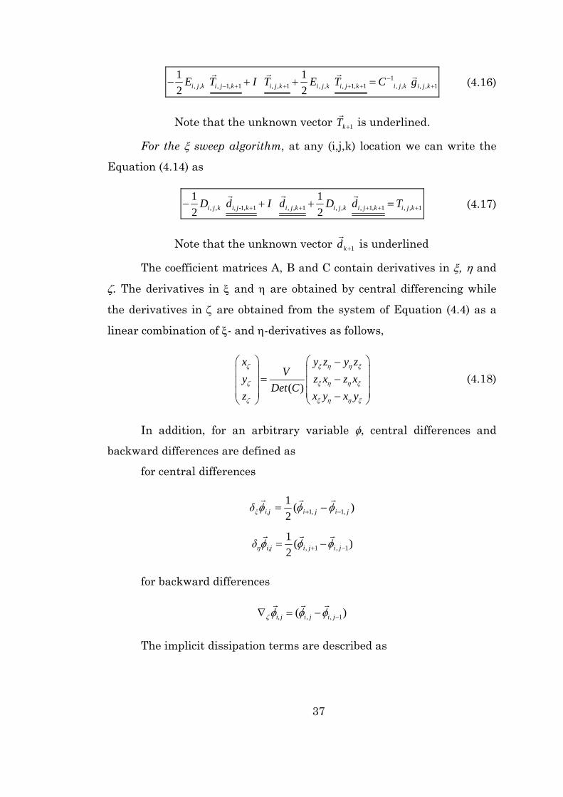
37

1, , , 1, 1 , , 1 , , , 1, 1 , , , , 1

1 1 2 2i j k i j k i j k i j k i j k i j k i j kE T I T E T C g−

− + + + + +− + + = (4.16)

Note that the unknown vector 1+kT is underlined.

For the ξ sweep algorithm, at any (i,j,k) location we can write the

Equation (4.14) as

, , 1, 1 , , 1 , , , 1, 1 , , 11 1 2 2i j k i, j- k i j k i j k i j k i j kD d I d D d T+ + + + +− + + = (4.17)

Note that the unknown vector 1+kd is underlined

The coefficient matrices A, B and C contain derivatives in ξ, η and

ζ. The derivatives in ξ and η are obtained by central differencing while

the derivatives in ζ are obtained from the system of Equation (4.4) as a

linear combination of ξ- and η-derivatives as follows,

( )

x y z y zVy z x z x

Det Cz x y x y

ζ ξ η η ξ

ζ ξ η η ξ

ζ ξ η η ξ

⎛ ⎞ ⎛ ⎞−⎜ ⎟ ⎜ ⎟

= −⎜ ⎟ ⎜ ⎟⎜ ⎟ ⎜ ⎟−⎝ ⎠ ⎝ ⎠

(4.18)

In addition, for an arbitrary variable φ, central differences and

backward differences are defined as

for central differences

)(

21

,1,1 jijii,jξδ −+ −= φφφ

)(

21

1,1, −+ −= jijii,jδ φφφη

for backward differences

, , 1( )i, j i j i jζφ φ φ −∇ = −

The implicit dissipation terms are described as

38

( ) ( )( ) ( )

1 1 1 12 2 2 2

1 1 1 12 2 2 2

11 12

11 12

i, j i, j i, j i, jj j j j

i, j i , j i, j i , ji i i i

η η

ξ ξ

ε φ β φ β β φ β φ

ε φ λ φ λ λ φ λ φ

+ −+ + − −

+ −+ + − −

∆∇ = − + +

∆∇ = − + + (4.19)

where

1

2

12

1

1

j jj

i ii

β β β

λ λ λ

±±

±±

=

=

4.2. Cell volume specification

In this method, the cell volumes from one grid point to the next

grid point for each level is prescribed simultaneously. One simple and

popular way to specify the cell volumes suggested in reference [69] is

,,,,,, kjikjikji sAV ∆∆=∆ (4.20)

where

: the grid point surface area, ,

: the marching spacing, ,

Ai j k

si j k

∆

∆

The marching distance, ∆si,j,k can be expressed as a function, which

matches the required criteria for the generated grid. For different

purposes, different functions can be used to specify the ∆s. In general, it is

obtained from the exponential function.

11,, )1( −+=∆ k

kji ss ε (4.21)

The values of s1 (initial grid spacing in the marching direction and

ε (the ratio of successive spacing in the marching direction) are the

required parameters.

39

4.3. Boundary Conditions

In general five types of implicit boundary conditions can be

incorporated in the three-dimensional code at the ξ and η boundaries [2].

As explained, the grids on the initial surface are defined in i=1 to imax

and j=1 to jmax, where imax and jmax are the maximum indices for i and

j.

Floating Edge Type of Boundary Condition that is used in the code

does not allow for the specification of any boundary information such as

edge shape or grid point distribution. Much as in the case of a constant

Cartesian plane, an entire ξ and η boundaries can be floated using the

simple hyperbolic equation 0=ξζr or 0=ηζr to update a boundary plane.

This is essentially a zeroth order extrapolation of ∆r from the adjacent

interior value.

4.4. An Example

As an illustrative example, the grid around Lann Wing [71] is

shown in Figure 4.1. Notice that Since floating type of boundary condition

is used, the boundaries splay outward.

40

XY

Z

Figure 4.1 Illustrative example of grid around Lann Wing [71]

XY

Z

Figure 4.2 Zoomed view

41

CHAPTER 5

ADAPTED TURBULENCE MODELS

5.1. Baldwin-Lomax Turbulence Model

The Baldwin and Lomax turbulence model [72] is an algebraic eddy

viscosity, zero equation model. The model is based on the mixing length

hypothesis. The model has been widely used and tested, and remains a

very popular turbulence model. Several advantages of the model are its

simplicity in coding and the fact that it does not require the boundary

layer edge thickness or edge velocity as an input parameter. The Baldwin

and Lomax model works best in wall-bounded flows with favorable

pressure gradients.

The calculation of eddy viscosity is not always straightforward and

can lead to errors in the turbulence model if not computed correctly. As

the flow physics become more complicated, as well as the geometry of the

model being tested, the performance of this turbulence model greatly

decreases.

The formulation is straightforward. It uses a two-layer algebraic

equation to calculate the eddy viscosity term, µt given by

( )( )

crossoverinner

crossoverouter

t

tt

µ y yµ

µ y y

≤⎧⎪= ⎨>⎪⎩

(5.1)

where y is the normal distance from the wall and ycrossover is the

location along the constant index line where ( )innertµ exceeds ( )outertµ ,

marching away from the wall.

For the inner region, µt is calculated as follows

42

2 2 2,inner Dk F tµ yρ= Ω (5.2)

where

VΩ = ∇×

( )( ) 1 exp / 26DF y y+⎡ ⎤= − −⎢ ⎥⎣ ⎦

w w

w

yρ τµ

+ =

where subscript ‘’w’’ denotes the ‘’wall‘’ quantities.

For the outer region, µt is calculated as follows.

,t outer cp wake klebKC F Fµ ρ= (5.3)

where

2max max max maxmin ; /wake wk diffF y F C y u F⎡ ⎤= ⎣ ⎦

16

max

1 5.5 klebkleb

C yFy

−⎡ ⎤⎛ ⎞⎢ ⎥= + ⎜ ⎟⎢ ⎥⎝ ⎠⎣ ⎦

( )1/ 22 2 2max min where diffu V V V u v w= − = + +

wk

kleb

K = 0.0168C = 0.25C = 0.3

Exponential term and Vmin is set to zero except in wakes. The value

Fmax is the maximum of the function F(y) defined as

( ) DF y y F= Ω (5.4)

and ymax is the value where F(ymax) =Fmax

43

5.2. Degani-Schiff Modification

For the flows around bodies, which experience cross flow

separations, maximum value of F(y) may be over predicted. This

modification attempts to select the first occurrence of Fmax in a search

from the wall outwards [73] , since the function F(y) exhibits more than

one peak in such a flows. For example in the case of separated flows, the

code must be forced to select the Fmax in the boundary layer otherwise it

may choose a length scale corresponding to the distance up to the rolling-

up vortices, which can be larger. The symptoms of this type of occurrence

may be stated as follows,

• Increase in the outer value of µt is too much,

• Details of the flow are distorted or washed out,

• Primary vortices are smaller,

• Primary separation is located closer to leeward symmetry plane,

• Secondary separation and vortices do not appear.

The code simply search and assigned the value of Fmax until the

following relation is satisfied

max0.9F F< (5.5)

5.3. Vorticity Adaptation

Often the vorticity from secondary sources is intermixed with the

wall bounded flow, which causes the turbulence model to predict the

value of "F" maximum incorrectly. This situation occurs with corner

flows, flows with near wall vortices and with globally swirling flows. The

Baldwin and Lomax model has been modified to calculate the "F" function

based on directionally correct vorticity vectors that are vorticity vectors

that are parallel to the local wall and perpendicular to the local velocity

vector. This use of a reduced vorticity vector has been shown to produce

dramatically improved prediction accuracy in some applications and has

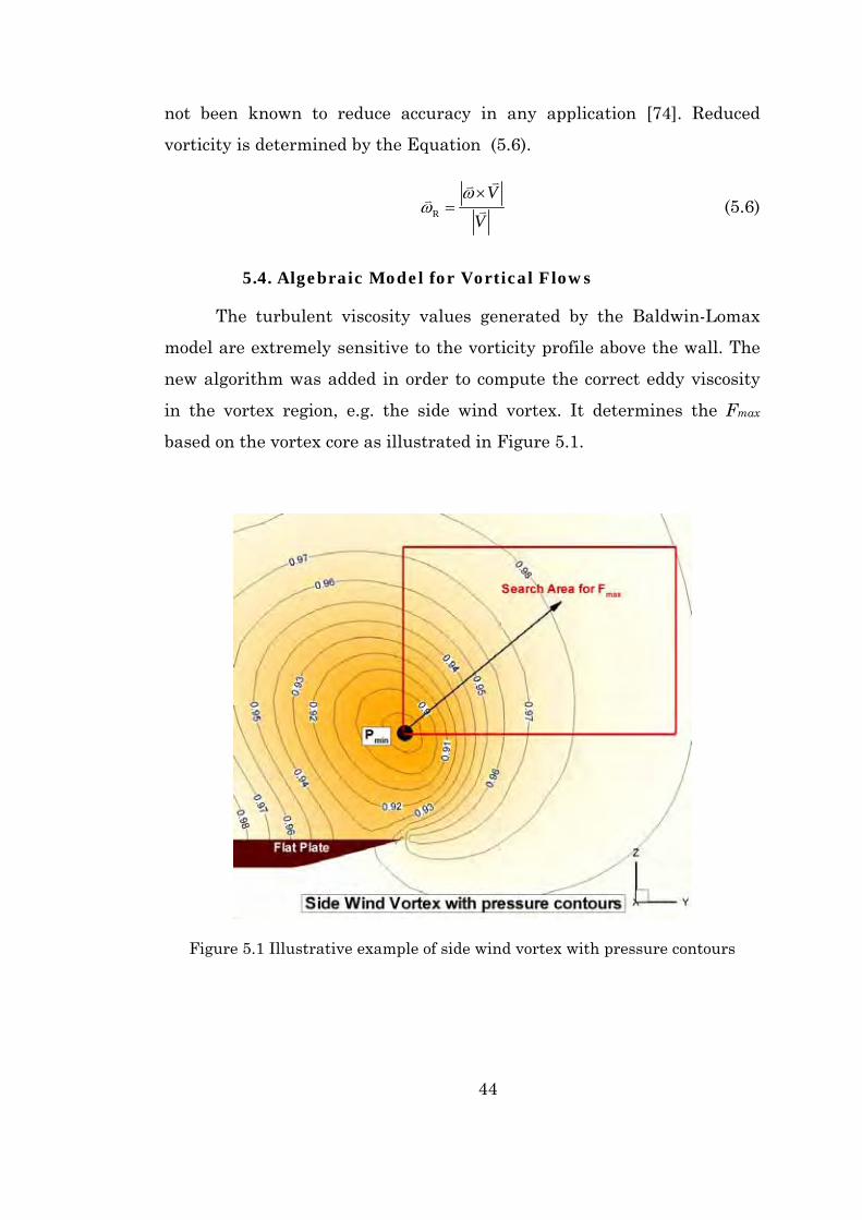
44

not been known to reduce accuracy in any application [74]. Reduced

vorticity is determined by the Equation (5.6).

R

V

V

ωω

×= (5.6)

5.4. Algebraic Model for Vortical Flows

The turbulent viscosity values generated by the Baldwin-Lomax

model are extremely sensitive to the vorticity profile above the wall. The

new algorithm was added in order to compute the correct eddy viscosity

in the vortex region, e.g. the side wind vortex. It determines the Fmax

based on the vortex core as illustrated in Figure 5.1.

Figure 5.1 Illustrative example of side wind vortex with pressure contours

45

The code first seeks the minimum pressure point, which is actually

the core of the vortex. Then it assigns this point as the starting point and

search for Fmax through the search area index by index.

5.5. Algebraic Wake Model

In order to use the simple algebraic models on block-structured

grids, the problem arises how to calculate the turbulent stresses in those

blocks that do not have a boundary layer- type flow, so that the model

was corrected to catch up the wake region. A typical example is the wake

of blunt bodies, because the algebraic models cannot calculate the

characteristic length and the velocity scale normal to the wall. Therefore,

empirical distribution laws were introduced to describe the turbulence

transport into these blocks [75]. Because the production of turbulent

energy in local equilibrium flows correlates with vorticity, this was taken

as a weighted function to distribute eddy-viscosity in that area, according

to

'vt t

v

αω

µ µω

⎛ ⎞= ⎜ ⎟⎜ ⎟

⎝ ⎠ (5.7)

with vt

µ the maximum eddy-viscosity along the upstream block face

and vω the local vorticity at that point. The exponent α is determined

by numerical experiments, as 0.2α = [75].

In addition, the eddy-viscosity is also smoothed by an exponential

damping factor in order to ensure steadiness on the block faces.

( )' '

max

exp jt t t t j

xx

µ µ µ µ∆⎛ ⎞

= − − −⎜ ⎟∆⎝ ⎠ (5.8)

where

46

t jµ ; the eddy-viscosity on the upstream block face at the same j-station as 'tµ

jx∆ ; the normal distance to the location of 'tµ

maxx∆ ; the length of the block in streamwise direction

47

CHAPTER 6

TEST CASES AND RESULTS

In this chapter, test cases will be covered in two main sections,

namely two dimensional test cases and three dimensional test cases

respectively. Results of each test case are presented in the corresponding

section.

6.1. Two Dimensional Test Cases

Two dimensional test cases are chosen to validate the Navier-

Stokes solver and to investigate the essential grid parameters for the

solution of three dimensional test cases.

6.1.1. Laminar Flat Plate

A grid convergence study of the PML3D code, for the solution of

laminar flow over a flat plate at zero incidence angle, is performed.

Comparisons are made between the computational results and the

analytical solution, which is the well known “The classical Blasius

similarity solution”, that provides data for comparison. Various textbooks

discuss this solution [77],[81]. The Reynolds number based on the free

stream velocity at distance from the plate leading edge, ranged from zero

to 2x106. The Reynolds number, ReL is equal to 1x106 at x/L=1.0. Three

different grids are produced and the effects of the grid on the accuracy of

the solution are observed. Number of iterations needed for a steady

converged solution is also investigated. For the numerical solution, The

Mach number of the flow is selected as Mach 0.4. On the other hand is

48

known that the Blasius solution is based on incompressible flow

assumption. When comparing the numerical and analytical results, is

assumed that compressibility effects are negligible for a boundary layer

flow at Mach=0.4. A laminar boundary layer develops on the plate and

thickens along the plate. The leading edge of flat plate is located at

coordinates (x/c=0, y/c=0).

x/c-1 -0.5 0 0.5 1 1.5 2

y/c

0

0.5Grid A

x/c-1 -0.5 0 0.5 1 1.5 2

y/c

0

0.5Grid B

x/c-1 -0.5 0 0.5 1 1.5 2

y/c

0

0.5Grid C

Figure 6.1 The applied grid geometries

6.1.1.1. Computational Grid and Initial Conditions

Single-block, two-dimensional, structured grids are generated for

the flow domain. There different grid configurations are used. The grid

geometries with actual dimensions (x/y aspect ratio = 1.0) are shown in

Figure 6.1 The grid parameters are shown in Table 6.1

49

Table 6.1 The grids used in the Computations

Grid Initial Grid Spacing

Density Maximum Marching Distance

A 6.25 E-5 60 x 80 0.545B 1.0 E-5 160 x 60 0.008C 1.0 E-5 160 x 130 0.03

In the grid configuration A, total of 4800 points were used as

shown in Figure 6.2. In the streamwise direction, 39 grid points were

used along the flat plate with the leading edge stretching. In the normal

direction, two different distribution were used; first 40 points were

distributed uniformly between plate surface and y/c = 0.0025 and then

stretched by tangent hyperbolic method. Initial grid spacing was set to

∆y/c = 6.25*E-5.

x/c-1 -0.5 0 0.5 1 1.5 2

y/c

0

0.1

0.2

0.3

0.4

0.5 Total 4800 points

39 points on the surface

60 points in streamwise 80 p

oint

s in

norm

al

∆y/c = 6.25*10-5

Figure 6.2 The grid configuration A

In the grid configuration B, total of 9600 points were used as

shown in Figure 6.3. In the streamwise direction, 139 grid points were

used along the flat plate with leading edge stretching. In the normal

50

direction, two different distribution were used again; first 40 points were

distributed by tangent hyperbolic stretching between plate surface and

y/c = 0.0025 and then stretched uniformly. Initial grid spacing was

preselected as ∆y/c = 1.0*E-5.

x/c-1 -0.5 0 0.5 1 1.5 2

y/c

0

0.002

0.004

0.006

0.008 Total 9600 points

139 points on the surface

160 points in streamwise 60 p

oint

s in

norm

al

∆y/c = 1.0*10-5

Figure 6.3. Grid configuration B

In the grid configuration C, total of 20800 points were used as

shown in Figure 6.4. In the streamwise direction, 139 grid points were

used again along the flat plate with leading edge stretching. In the

normal direction, first 65 points were distributed by tangent hyperbolic

stretching between plate surface and y/c = 0.0025 and then stretched in

the same manner. Initial grid spacing was preselected as ∆y/c = 1.0*E-5.

51

x/c-1 -0.5 0 0.5 1 1.5 2

y/c

0

0.005

0.01

0.015

0.02

0.025

0.03 Total 20800 points

139 points on the surface

160 points in streamwise 130

poin

ts in

nor

mal

∆y/c = 1.0*10-5

Figure 6.4. Grid configuration C

6.1.1.2. Boundary Conditions

At the flat plate surface, the no-slip condition applies. The inflow

boundary of the computational domain is a subsonic inflow boundary and

is placed upstream of the leading edge at x/c = - 1 so as to capture the

leading edge flow. The outflow boundary is placed at the end of the plate

at x/c = 2.0. The farfield flow beyond the boundary layer should remain

fairly uniform at freestream conditions. The farfield boundary is placed

according to the applied grid configuration.

Table 6.2 Computational details

Grid CPU time (minute)

Memory Requirement

(Mb)

Number of Points

Number of Iterations

A 91 7388 4800 40000B 190 9416 9600 40000C 1380 16000 20800 100000

52

6.1.1.3. Computational Studies

The computation starts from the freestream solution and marches

in time using local time-stepping until the L2 residual has leveled off. A

constant CFL number of 30 is used. The steady-state flow was computed

for each grid.

For the grid configurations A and B, 40000 iteration steps were

required for a steady-state solution. However, the case belonging to the

grid configuration C converged fully at 100000 iterations. Computations

are performed on P4 1500 MHz single processor workstation. The

computational details are given in Table 6.2.

6.1.1.4. Convergence History

In Figure 6.5, the convergence history for all cases is shown in

terms of L2 Residual. For the first two cases, although the solution was

converged after the 40000 iteration steps, L2 norm continues to drop. .

From that figure, it can be seen that, after 70000 iterations, the solution

with Grid A has converged 18 orders of magnitude, the solution with Grid

B has converged 6.5 orders of magnitude, and the solution with the Grid

C after 100000 iterations has converged 4.5 orders of magnitude. In

normal conditions, three orders of magnitude convergence is accepted to

be sufficient for a converged solution.

53

Iterations

L 2

0 20000 40000 60000 80000 100000

10-25

10-20

10-15

10-10

GRID-AGRID-BGRID-C

Figure 6.5 Convergence history, L2 Norm of Residue

Table 6.3 Blasius solution [77].

Skin Friction Coefficient 1/ 2

0.664f

x

cRe

=

Boundary Layer Thickness 1/ 2

5

xx Reδ=

Displacement Thickness *

1/ 2

1.721

xx Reδ

=

Momentum Thickness 1/ 2

0.664

xx Reθ=

Shape Parameter 59.2*

==θδH

54

6.1.1.5. Comparisons of the results

The computed flow properties such as pressure coefficient, skin

friction coefficient, boundary layer thickness, momentum thickness,

shape factor etc. are compared to the analytic results of Blasius [77]

shown in Table 6.3 to establish the validity of the computed results.

The difference in the flow domain especially the boundary layer

explicitly shows the validity and the accuracy of the applied grids. These

are shown in Figure 6.6, Figure 6.7 and Figure 6.8 for each case with an

exaggerated view such that the dependency between the axes is

temporarily removed. Notice that the number of points that were placed

on the flat plate surface in the normal direction at various locations lying

on the boundary layer. For the Grid A and B, picture seems to be the

same but the results shows that the number of points in the streamwise

direction has an important role about the accuracy of the problem.

Moreover, they have too small number of points for the first quarter of

the flat plate. Hence, the Grid C seems to be capable of capturing the flow

properties through the boundary layer.

55

Figure 6.6 The boundary layer for grid A

Figure 6.7 Boundary layer for grid B

56

Figure 6.8 Boundary layer for grid C

The following figures show the comparison of the computational

and analytic results of the selected variables. The computational results

are taken from the fully converged solutions of each case.

Figure 6.9, Figure 6.10 and Figure 6.11 shows the iterative

convergence of the parameter Cf for each grid respectively. The results in

these figures have belonging to the conditions at 70000 iterations for A

and B type Grids and 100000 iterations for C type Grids.

57

Rex

CfR

e x0.5

5.0E+05 1.0E+06 1.5E+06 2.0E+060.5000

0.6000

0.7000

0.8000

0.9000

1.0000

1.1000

10000

40000-70000

20000

30000Blasius

Iterative Convergencefor the Grid-A Solution

Figure 6.9 Iterative convergence of the grid-A solution

Rex

CfR

e x0.5

5.0E+05 1.0E+06 1.5E+06 2.0E+060.5000

0.6000

0.7000

0.8000

0.9000

1.0000

1.1000

10000

50000-70000

20000

30000

Blasius

Iterative Convergencefor the Grid-B Solution

40000

Figure 6.10 Iterative convergence of the grid-B solution

58

Rex

CfR

e x0.5

5.0E+05 1.0E+06 1.5E+06 2.0E+06

0.6000

0.7000

0.8000

0.9000

1.0000

1.1000

1.2000

1.3000

1.4000

1000

040000

20000

70000

50000

100000

30000

60000

Blasius

Iterative Convergencefor the Grid-C Solution

Figure 6.11 Iterative convergence of the grid-C solution

Rex

Cp

0.0E+00 5.0E+05 1.0E+06 1.5E+06 2.0E+06-0.0100

-0.0050

0.0000

0.0050

0.0100

Grid-AGrid-BGrid-CBlasius

Figure 6.12 Pressure coefficient comparison

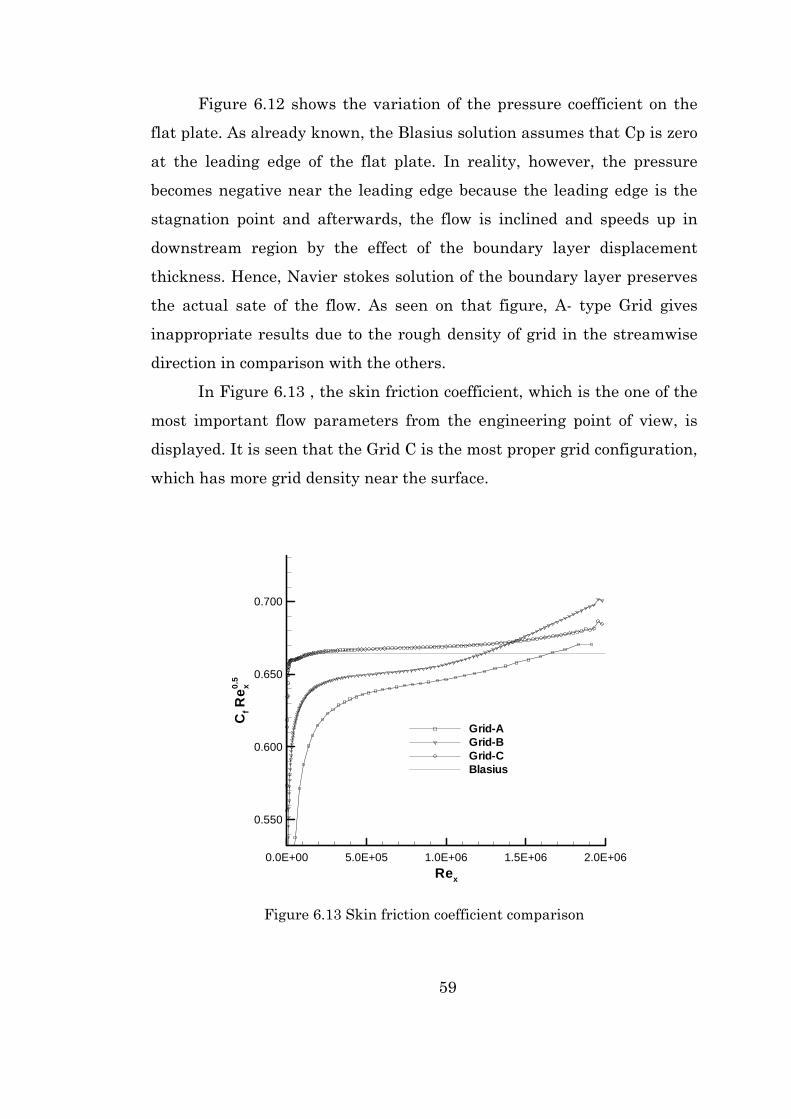
59

Figure 6.12 shows the variation of the pressure coefficient on the

flat plate. As already known, the Blasius solution assumes that Cp is zero

at the leading edge of the flat plate. In reality, however, the pressure

becomes negative near the leading edge because the leading edge is the

stagnation point and afterwards, the flow is inclined and speeds up in

downstream region by the effect of the boundary layer displacement

thickness. Hence, Navier stokes solution of the boundary layer preserves

the actual sate of the flow. As seen on that figure, A- type Grid gives

inappropriate results due to the rough density of grid in the streamwise

direction in comparison with the others.

In Figure 6.13 , the skin friction coefficient, which is the one of the

most important flow parameters from the engineering point of view, is

displayed. It is seen that the Grid C is the most proper grid configuration,

which has more grid density near the surface.

Rex

CfR

e x0.5

0.0E+00 5.0E+05 1.0E+06 1.5E+06 2.0E+06

0.550

0.600

0.650

0.700

Grid-AGrid-BGrid-CBlasius

Figure 6.13 Skin friction coefficient comparison

60

Results of the boundary layer thickness parameters are shown in

Figure 6.14, Figure 6.15, and Figure 6.16. The computed boundary layer

thickness δ is defined as the distance from the plate where max0.99u u= × ,

where umax is the value at the first maximum in the u profile. The

momentum and displacement thicknesses were computed from the

standard 2-D planar definitions.

*

0

1my u dy

uδ

∞

⎛ ⎞= −⎜ ⎟

⎝ ⎠∫ (6.1)

0

1my u u dy

u uρθρ∞ ∞ ∞

⎛ ⎞= −⎜ ⎟

⎝ ⎠∫ (6.2)

where ym is the distance from the plate to the first maximum in u.

Simpson's rule was used for the numerical integration. The shape factor

is simply defined as H = δ*/ θ.

In order to detect the thickness parameters correctly, the grid

density must be sufficient in either directions, streamwise and normal,

especially in the boundary layer region. Coarse grids around the

boundary layer edge may lead to weak prediction of boundary layer

thickness. The grid C, which has more grid points in both direction,

correctly detects the parameters involved. The boundary layer shape

parameter, H, is presented in Figure 6.17.

61

Rex

(δ/x

)Re x0.

5

5.0E+05 1.0E+06 1.5E+06 2.0E+06

4.5

5.0

5.5

6.0

6.5

7.0

7.5

Grid-AGrid-BGrid-CBlasius

Figure 6.14 Boundary layer thickness comparison

Rex

(δ* /x

)Re x0.

5

0.0E+00 5.0E+05 1.0E+06 1.5E+06 2.0E+061.5

1.6

1.7

1.8

1.9

2.0

Grid-AGrid-BGrid-CBlasius

Figure 6.15 Displacement thickness comparison

62

Rex

(θ/x

)Re x0.

5

0.0E+00 5.0E+05 1.0E+06 1.5E+06 2.0E+06

0.4

0.6

0.8

1.0

Grid-AGrid-BGrid-CBlasius

Figure 6.16 Momentum thickness comparison

Rex

H

5.0E+05 1.0E+06 1.5E+06 2.0E+062.0

2.5

3.0

3.5

4.0

Grid-AGrid-BGrid-CBlasius

Figure 6.17 Shape parameter comparison

63

In this study, the grid effects were investigated on the Navier-

Stokes solution of the boundary layer. It was seen that the solution was

effected by the following parameters; the grid density of the boundary

layer in the normal direction to the flow, the minimum grid spacing and

the grid density in the streamwise direction. By using less dense grid in

the solution, it is seen that L2 residual is decreasing steeply but

converging to the less accurate results. On the other hand, in the case of

using more dense grid in appropriate regions, L2 residual is decreasing

slowly but converging to the more accurate results. In addition, it is

understood that the flow solver, which is specifically coded for

compressible flows, converges slowly for low speed viscous flows but can

give accurate results when a proper grid is used.

64

6.1.2. Turbulent Flat Plate

Turbulent flow over a flat plate at zero incidence was investigated.

Compressibility effects are neglected during study so that the results are

compared with the incompressible experimental data. The Reynolds

number, ReL is equal to 1x107. The Reynolds number based on the free

stream velocity at distance from the plate leading edge, ranged from zero

to 2x107 .

6.1.2.1. Computational Grid and Initial Conditions

The computational mesh was generated by using hyperbolic grid

generation code [76]. Grid points in the streamwise direction were packed

near the leading edge with a total number of points 160 and 140 of them

are distributed along the flat plate.

At the normal direction, 96 points were used with 71 points in the

boundary layer. The boundary layer thickness was estimated as follows

[77].

1/5

0.38Rex

xδ = (6.3)

Marching distance was arranged as to follow the boundary layer

thickness along the flat plate using a Roberts’s transformation [78]. With

this transformation, for a line of length D, points are packed near the

beginning of the line.

The distance between solid wall and the first grid point was

prescribed as follows. At least one grid point was placed where y+ was

equal to 1.0. Pre-studies showed that for a mesh that follows the

boundary layer, the right place of y+ analysis was the trailing edge of the

plate, or the exit plane. If at least one grid point was placed where y+ was

equal to 1.0 at that region, then it was guaranteed that there is more grid

point at the leading edge region where y+ was equal to 1.0.

65

y+ analysis is conducted by using the following equation,

2

fL

cyy Rec

+ ⎛ ⎞= ⎜ ⎟⎝ ⎠

(6.4)

where cf is the skin friction coefficient and ReL is the Reynolds

number.

The value of cf was estimated through the Schoenherr formula [77]

as follows:

1 4.15log( ) 1.7x ff

Re cc

= + (6.5)

For our case, Rex was 2x107 at exit section of the plate. Then

according to the above formula, cf was found to be 0.002264. By Equation

(6.5), the minimum value of y/c was then found to be 2.972x10-6. For the

outer region expect from boundary layer, the points were stretched

geometrically until the upper computational boundary was at

approximately, y96 = 7δ. As a result, the value of y+ at the first grid point

was estimated as ranging from about 0.2 near the leading edge of the

plate, to about 1.0 at the exit plane.

The resulting grid, scaled to fit is shown in Figure 6.18. The edge of

the boundary layer, as predicted by equation 2, is shown as a thick/black

line. Figure 6.19 shows the grid with no scaling. In addition, zoomed view

at the beginning of the boundary layer slope is shown in Figure 6.20.

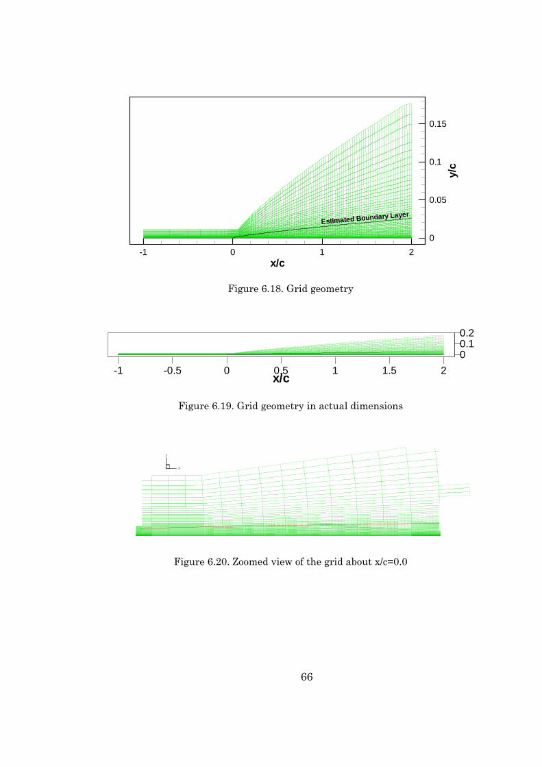
66

x/c-1 0 1 2

y/c

0

0.05

0.1

0.15

Estimated Boundary Layer

160x96

Figure 6.18. Grid geometry

x/c-1 -0.5 0 0.5 1 1.5 200.10.2

Figure 6.19. Grid geometry in actual dimensions

Y X

Z

Figure 6.20. Zoomed view of the grid about x/c=0.0

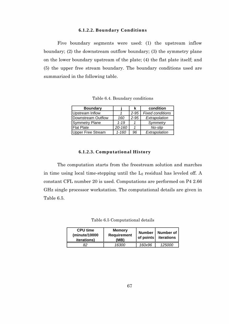
67

6.1.2.2. Boundary Conditions

Five boundary segments were used: (1) the upstream inflow

boundary; (2) the downstream outflow boundary; (3) the symmetry plane

on the lower boundary upstream of the plate; (4) the flat plate itself; and

(5) the upper free stream boundary. The boundary conditions used are

summarized in the following table.

Table 6.4. Boundary conditions

Boundary j k conditionUpstream Inflow 1 2-95 Fixed conditionsDownstream Outflow 160 2-95 ExtrapolationSymmetry Plane 1-19 1 SymmetryFlat Plate 20-160 1 No-slipUpper Free Stream 1-160 96 Extrapolation

6.1.2.3. Computational History

The computation starts from the freestream solution and marches

in time using local time-stepping until the L2 residual has leveled off. A

constant CFL number 20 is used. Computations are performed on P4 2.66

GHz single processor workstation. The computational details are given in

Table 6.5.

Table 6.5 Computational details

CPU time (minute/10000

iterations)

Memory Requirement

(MB)

Number of points

Number of iterations

82 16300 160x96 125000

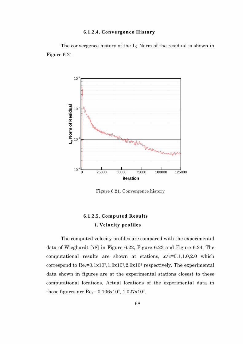
68

6.1.2.4. Convergence History

The convergence history of the L2 Norm of the residual is shown in

Figure 6.21.

iteration

L 2N

orm

ofR

esid

ual

0 25000 50000 75000 100000 12500010-9

10-8

10-7

10-6

Figure 6.21. Convergence history

6.1.2.5. Computed Results

i. Velocity profiles

The computed velocity profiles are compared with the experimental

data of Wieghardt [78] in Figure 6.22, Figure 6.23 and Figure 6.24. The

computational results are shown at stations, x/c=0.1,1.0,2.0 which

correspond to Rex=0.1x107,1.0x107,2.0x107 respectively. The experimental

data shown in figures are at the experimental stations closest to these

computational locations. Actual locations of the experimental data in

those figures are Rex= 0.106x107, 1.027x107.

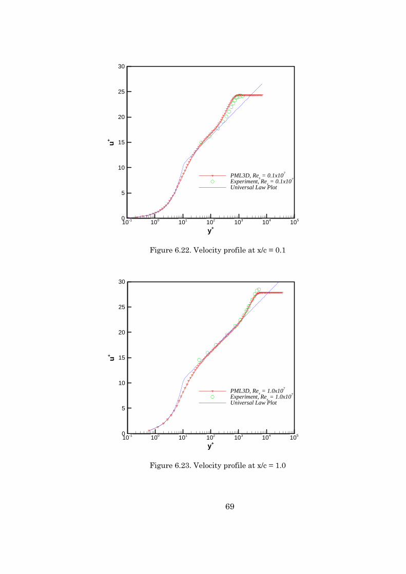
69

y+

u+

10-1 100 101 102 103 104 1050

5

10

15

20

25

30

PML3D, Rex = 0.1x107

Experiment, Rex = 0.1x107

Universal Law Plot

Figure 6.22. Velocity profile at x/c = 0.1

y+

u+

10-1 100 101 102 103 104 1050

5

10

15

20

25

30

PML3D, Rex = 1.0x107

Experiment, Rex = 1.0x107

Universal Law Plot

Figure 6.23. Velocity profile at x/c = 1.0

70

y+

u+

10-1 100 101 102 103 104 1050

5

10

15

20

25

30

PML3D, Rex = 2.0x107

Universal Law Plot

Figure 6.24. Velocity profile at x/c = 2.0

ii. Thickness Parameters

In Figure 6.25 through Figure 6.28, computed values of boundary

layer thickness δ, momentum thickness θ, displacement thickness δ* ,

and shape factor H, respectively are compared with the correlation values

based on simple power-law analyses [77], [81].

71

Distance, Rex

Bou

ndar

yLa

yerT

hick

ness

,δ/x

0.0x10+00 4.0x10+06 8.0x10+06 1.2x10+07 1.6x10+07 2.0x10+070.00

0.02

0.04

0.06

0.08

0.10

PML3D ComputationCorrelation, δ/x=0.37Rex

-1/5

Figure 6.25. Boundary layer thickness

Distance, Rex

Mom

entu

mTh

ickn

ess,θ/

x

0.0x10+00 4.0x10+06 8.0x10+06 1.2x10+07 1.6x10+07 2.0x10+070.000

0.002

0.004

0.006

0.008

0.010

PML3D ComputationCorrelation, θ/x = 0.036Rex

-1/5

Figure 6.26. Momentum thickness

72

Distance, Rex

Dis

plac

emen

tThi

ckne

ss,δ

∗ /x

0.0x10+00 4.0x10+06 8.0x10+06 1.2x10+07 1.6x10+07 2.0x10+070.000

0.002

0.004

0.006

0.008

0.010

PML3D ComputationCorrelation, δ∗/x = 0.046Rex

-1/5

Figure 6.27. Displacement thickness

Distance, Rex

Sha

peFa

ctor

,H

0.0x10+00 4.0x10+06 8.0x10+06 1.2x10+07 1.6x10+07 2.0x10+071.00

1.20

1.40

1.60

1.80

2.00

PML3D ComputationCorrelation, H = 1.278

Figure 6.28. Shape factor

73

iii. Skin Friction

The computed skin friction coefficient is compared with values from

two different correlation formulas [77], [81] in Figure 6.29.

Distance, Rex

Ski

nFr

ictio

nC

oeffi

cien

t,c f

0.0x10+00 4.0x10+06 8.0x10+06 1.2x10+07 1.6x10+07 2.0x10+070.000

0.002

0.004

0.006

0.008

0.010

PML3D ComputationCorrelation, cf = 0.0592*Rex

-0.2

Correlation, cf = 0.455 / ln20.06Rex

Figure 6.29. Skin friction coefficient

74

6.2. Three Dimensional Flat Plate

6.2.1. Problem Description

For the present computational study, an aspect ratio 1.0 flat plate

with small thickness and sharp edges is considered as the test model. The

computational test matrix given in Table 6.6 is constructed according to

the experiment data [39]. The cases P1-P4 are intended for pressure

comparisons and the cases S1, S2 are intended for surface streamline

comparisons with experiments.

Table 6.6 Computational test matrix

CASE M∞ Re∞ α (deg)

P1 0.54 3.0*105 7.5

P2 0.55 3.0*105 13.5

P3 0.87 3.0*105 7.5

P4 0.85 3.0*105 13.5

S1 0.42 1.65*105 5.0

S2 0.42 1.65*105 15.0

The flow domain is composed of two zones namely Block-1 and

Block-2 as seen on Figure 6.31. According to the researchers in high angle

of attack aerodynamics [2], [3] , vortex asymmetry begins when the angle

of attack is about twice the nose angle. As a rough estimate, it is may be

75

guaranteed that vortex asymmetry does not exist until the angle of attack

is about 23 degree. In our test cases, the nose angle is 15 degree and the

angle of attack varies from 5o to 15o. Moreover, the experiments [39]

about our test cases report that the flow is symmetric. Hence, we can

consider that the flow field is symmetric with respect to the xz plane, and

then apply the computation over only the half of the flat plate.

Figure 6.30 Computational flow domain

The first zone is above the flat plate and extends in the range of

-3.0 / 4.0x c≤ ≤ , 0.0 / 3.5y c≤ ≤ and 0.0 / 3.0z c≤ ≤ . The second zone is

below the flat plate and extends in the range of -3.0 / 4.0x c≤ ≤ ,

0.0 / 3.5y c≤ ≤ and 3.0 / 0.0z c− ≤ ≤ . The flat plate lies in the 0.0z = plane

76

and it extends in the range of 0.0 / 1.0x c≤ ≤ and 0.0 / 0.5y c≤ ≤ . The flat

plate has a three dimensional geometry, which has four sharp edges as

shown in Figure 6.31.

Figure 6.31 Computational flat plate geometry

8 0

8

1 8

80

40

1 5 3 . 2 3

Figure 6.32 Model used for compressible oil flow tests [10].

77

6.2.2. Experimental Data For Comparison

The test cases are selected from the experimental data acquired at the

von Karman Institute (VKI) [38], [39]. Test models are low aspect ratio,

rectangular flat plates with small thickness and sharp edges. Model aspect

ratios (AR) are 0.5, 0.67, 1.0 and 1.5. For AR=1.0, the low speed model

dimensions are 100mm*100mm*5mm. This model was used for low speed oil

flow visualization tests. The high-speed force model dimensions are

80mm*80mm*2mm. The high-speed pressure model dimensions are

100m*100mm. Front and side edges of the models are sharp. The top surfaces

of the models are not deflected at the edges and connected to the lower

surfaces with 15° angle. In Figure 6.32, the top and side view drawings of the

model used for high-speed oil flow measurements are shown.

The experiments include surface oil flow measurements, force and

moment measurements and surface pressure distribution measurements.

Low speed tests were carried out in the VKI low speed, open circuit wind

tunnel of the suction type, designated L-2A. This tunnel has a 0.3 m

diameter circular test section. Maximum tunnel velocity is 40 m/sec and

the Reynolds number based on the model chord length is about 2*105. At

low speeds, oil flow visualizations were performed at different angles of

attack varying from 0° to 40°. High-speed subsonic tests were carried out

in the VKI S-1 wind tunnel. This is a closed circuit transonic / supersonic

wind tunnel with 0.4 m * 0.4 m test section. Subsonic tests are performed

in the transonic test section with slotted horizontal walls. High-speed

tests include surface pressure distribution measurements, force and

moment measurements and a few oil flow measurements. Mach number

range was 0.4-0.9. Reynolds numbers varied between 1.63x105 and

2.62x105.

78

6.2.3. Computational Grid

η

ξ

ζξ

ζη

XY

Z

Block-2100x50x70

Block-1100x50x70

Figure 6.33 Overall view of the grid blocks, Block-1 and Block-2

Two-block, three-dimensional, structured grids shown in Figure

6.33 were generated for the computational flow domain mentioned above.

In order to speed up the convergence of the solutions, two different grid

configurations are adapted namely, the coarse and the fine grids. The

coarse grid is obtained by halving the number of grid points of the fine

grid in each coordinate direction. A three dimensional hyperbolic grid

generation code [76] is employed to generate the grids. The grid

parameters are shown in Table 6.7.

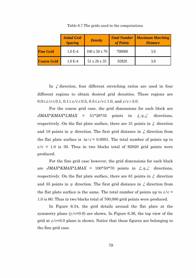
79

Table 6.7 The grids used in the computations

Initial Grid Spacing Density Total Number

of PointsMaximum Marching

Distance

Fine Grid 1.0 E-4 100 x 50 x 70 700000 3.0

Coarse Grid 1.0 E-4 51 x 26 x 35 92820 3.0

In ζ direction, four different stretching ratios are used in four

different regions to obtain desired grid densities. These regions are

0.0≤ z/c≤0.1, 0.1≤ z/c≤0.5, 0.5≤ z/c≤1.0, and z/c>3.0.

For the coarse grid case, the grid dimensions for each block are

JMAX*KMAX*LMAX = 51*26*35 points in , ,ξ η ζ directions,

respectively. On the flat plate surface, there are 31 points in ξ direction

and 18 points in η direction. The first grid distance in ζ direction from

the flat plate surface is /z c∆ = 0.0001. The total number of points up to

z/c = 1.0 is 30. Thus in two blocks total of 92820 grid points were

produced.

For the fine grid case however, the grid dimensions for each block

are JMAX*KMAX*LMAX = 100*50*70 points in , ,ξ η ζ directions,

respectively. On the flat plate surface, there are 61 points in ξ direction

and 35 points in η direction. The first grid distance in ζ direction from

the flat plate surface is the same. The total number of points up to z/c =

1.0 is 60. Thus in two blocks total of 700,000 grid points were produced.

In Figure 6.34, the grid details around the flat plate at the

symmetry plane (y/c=0.0) are shown. In Figure 6.36, the top view of the

grid at z/c=0.0 plane is shown. Notice that those figures are belonging to

the fine grid case.

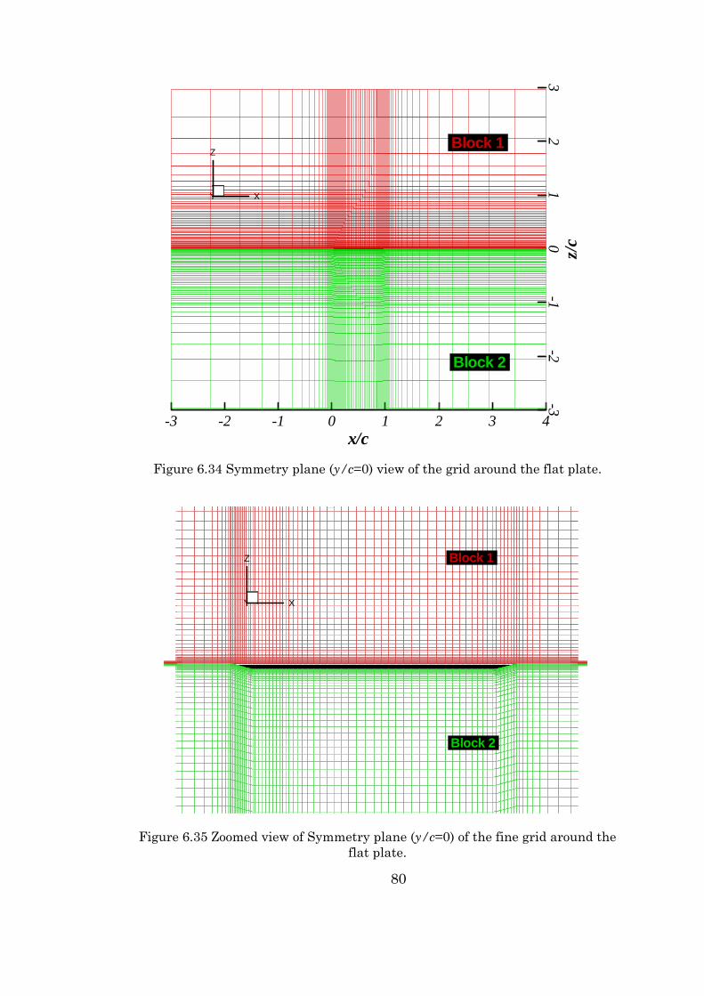
80

x/c-3 -2 -1 0 1 2 3 4

z/c

-3-2

-10

12

3

Y X

Z

Block 2

Block 1

Figure 6.34 Symmetry plane (y/c=0) view of the grid around the flat plate.

Y X

Z

Block 2

Block 1

Figure 6.35 Zoomed view of Symmetry plane (y/c=0) of the fine grid around the flat plate.

81

x/c-3 -2 -1 0 1 2 3 4

y/c

01

23

X

Y

Z

Top view

Figure 6.36 Top view of the grid at z/c=0.0 plane.

6.2.4. Boundary Conditions

Five different types of boundary conditions are used in each block as

shown in Figure 6.37: (1) the upstream inflow boundaries; (2) the downstream

outflow boundaries; (3) the symmetry boundary at the symmetry plane

(y/c=0); (4) the flat plate itself and (5) the matched surface boundary.

The upstream inflow boundary condition or inflow bc is fixed by the

freestream values. The downstream outflow boundary conditions, or

extrapolation bc are just extrapolated from the interior values. The no-

slip condition, or surface bc is applied on the flat plate surface. In the

matched surface boundary, the values are interchanged instantly

between two blocks by means of parallel processing. The boundary

conditions used in Fine Grid solution of each block are summarized in the

following table.

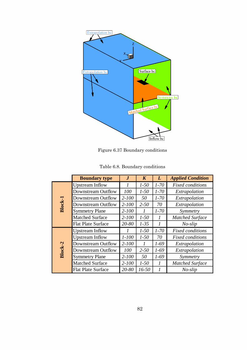
82

Figure 6.37 Boundary conditions

Table 6.8. Boundary conditions

Boundary type J K L Applied ConditionUpstream Inflow 1 1-50 1-70 Fixed conditionsDownstream Outflow 100 1-50 1-70 ExtrapolationDownstream Outflow 2-100 50 1-70 ExtrapolationDownstream Outflow 2-100 2-50 70 ExtrapolationSymmetry Plane 2-100 1 1-70 SymmetryMatched Surface 2-100 1-50 1 Matched SurfaceFlat Plate Surface 20-80 1-35 1 No-slipUpstream Inflow 1 1-50 1-70 Fixed conditionsUpstream Inflow 1-100 1-50 70 Fixed conditionsDownstream Outflow 2-100 1 1-69 ExtrapolationDownstream Outflow 100 2-50 1-69 ExtrapolationSymmetry Plane 2-100 50 1-69 SymmetryMatched Surface 2-100 1-50 1 Matched SurfaceFlat Plate Surface 20-80 16-50 1 No-slip

Blo

ck-1

Blo

ck-2

83

6.2.5. Solution Procedure

As mentioned above, two different, the coarse and the fine grid

configurations are utilized in order to get fast convergence of the solution.

All cases (P1, P2, P3, P4, S1 and S2) were solved over the coarse

grid by using a local time step (i.e., varying in space) with a CFL number

of 20. For each Case, coarse grid solution procedures decided by the

convergence criteria of the flow variables are as follows;

P1 Case was obtained for 40000 iterations using the Baldwin-

Lomax turbulence model applied over the region: x/c>0.30 of the flat

plate.

P2 Case was obtained for 41000 iterations using the Baldwin-

Lomax turbulence model applied over the complete flat plate surface.

P3 Case was obtained by applying the Baldwin-Lomax turbulence

model;

→ for the first 35000 iterations over the region; x/c>0.30

→ for the next 5000 iterations over the complete flat plate surface.

P4 Case was obtained for 66000 iterations using the Baldwin-

Lomax turbulence model applied over the complete flat plate surface.

S1 Case was obtained for 45000 iterations using the Baldwin-

Lomax turbulence model applied over the region: x/c>0.30 of the flat

plate.

S2 Case was obtained for 40000 iterations using the Baldwin-

Lomax turbulence model applied over the complete flat plate surface.

The fine grid solutions were initialized by the interpolation of those

coarse grid results. P1 and S1 Cases were obtained by applying the

Baldwin-Lomax turbulence model over the region; x/c>0.3 of the flat

plate surface and the rest were all over of the complete flat plate surface.

The iteration summary is given in Table 6.9

84

Table 6.9 Iteration summary

P1 P2 P3 P4 S1 S2 Course Grid iterations 40000 41000 40000 66000 44750 40000

Fine Grid iterations 29300 21500 20750 74000 21800 82500total 69300 62500 60750 140000 66550 122500

In the fine grid solutions, however, the time step was shifted to the

global time step (i.e., constant in space) since the results showed that

unsteady phenomena’s were taking place such as oscillating of Normal

Force and Pitching Moment, etc. The flow code computes the

corresponding time step at every point in the grid, finds the minimum of

those time steps, and resets the time step at every point to that minimum

value. This allows the time step to be set for an unsteady flow problem by

specifying a CFL number. Hence, approximately 20000-30000 more

iterations for all cases were required for the convergence of the flow

variables. This was achieved by tracing back the behavior of the flow

variables until reaching a periodic oscillation for each case study. 20

samples of each solution over one cycle were saved in order to determine

the time-mean average of each flow variable and visualize the flow

oscillations and instabilities.

6.2.6. Computational Details

Computations are performed on Pentium IV 1500 MHz single

processor workstation, which has 512 MB of memory. For coarse grid, a

two-block parallel solution with 2*46410 grid points requires 2*16 MB of

RAM. Approximately 240 minutes of CPU-time is needed per 10000

iterations. On the other hand, for fine grid, a two-block parallel solution

with 2*350000 grid points requires 2*82 MB of RAM and approximately

1600 minutes of CPU-time is needed per 10000 iterations. The

computational details are given in Table 6.10.

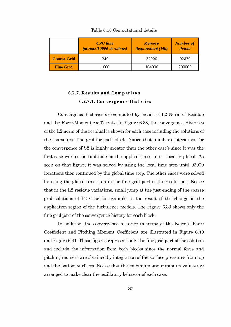
85

Table 6.10 Computational details

CPU time (minute/10000 iterations)

Memory Requirement (Mb)

Number of Points

Course Grid 240 32000 92820

Fine Grid 1600 164000 700000

6.2.7. Results and Comparison

6.2.7.1. Convergence Histories

Convergence histories are computed by means of L2 Norm of Residue

and the Force-Moment coefficients. In Figure 6.38, the convergence Histories

of the L2 norm of the residual is shown for each case including the solutions of

the coarse and fine grid for each block. Notice that number of iterations for

the convergence of S2 is highly greater than the other case’s since it was the

first case worked on to decide on the applied time step ; local or global. As

seen on that figure, it was solved by using the local time step until 93000

iterations then continued by the global time step. The other cases were solved

by using the global time step in the fine grid part of their solutions. Notice

that in the L2 residue variations, small jump at the just ending of the coarse

grid solutions of P2 Case for example, is the result of the change in the

application region of the turbulence models. The Figure 6.39 shows only the

fine grid part of the convergence history for each block.

In addition, the convergence histories in terms of the Normal Force

Coefficient and Pitching Moment Coefficient are illustrated in Figure 6.40

and Figure 6.41. Those figures represent only the fine grid part of the solution

and include the information from both blocks since the normal force and

pitching moment are obtained by integration of the surface pressures from top

and the bottom surfaces. Notice that the maximum and minimum values are

arranged to make clear the oscillatory behavior of each case.

86

iterations

Res

idue

0 10000 20000 30000 40000 50000 6000010-10

10-9

10-8

10-7

10-6

10-5

L2 Block 1L2 Block 2

Case P3M=0.87 α=7.5o

iterations

Res

idue

0 10000 20000 30000 40000 50000 6000010-10

10-9

10-8

10-7

10-6

10-5L2 Block 1L2 Block 2

Case P2M=0.55 α=13.5o

iterations

Res

idue

0 25000 50000 75000 100000 12500010-8

10-7

10-6

10-5

L2 Block 1L2 Block 2

Case P4M=0.85 α=13.5o

iterations

Res

idue

0 10000 20000 30000 40000 50000 6000010-10

10-9

10-8

10-7

10-6

10-5

L2 Block 1L2 Block 2

Case S1M=0.42 α=5.0o

iterations

Res

idue

0 25000 50000 75000 100000 12500010-20

10-18

10-16

10-14

10-12

10-10

10-8

L2 Block 1L2 Block 2

Case S2M=0.42 α=15o

iterations

Res

idue

0 10000 20000 30000 40000 50000 6000010-10

10-9

10-8

10-7

10-6

10-5 L2 Block 1L2 Block 2

Case P1M=0.54 α=7.5o

Figure 6.38 Convergence histories for the coarse and fine grid for each Case

87

iterations

Res

idue

40000 45000 50000 55000 60000

1E-06

2E-06

3E-06

4E-065E-06

L2 Block 1L2 Block 2

Case P3M=0.87 α=7.5o

iterations

Res

idue

40000 45000 50000 55000 60000 65000

5E-07

1E-06

1.5E-062E-06

2.5E-06

L2 Block 1L2 Block 2

Case P1M=0.54 α=7.5o

iterations

Res

idue

40000 45000 50000 55000 60000 65000

1E-06

2E-06

3E-06

4E-06

5E-06

L2 Block 1L2 Block 2

Case P2M=0.55 α=13.5o

iterations

Res

idue

100000 110000 120000 130000

1E-07

2E-07

3E-07

4E-075E-076E-077E-07

L2 Block 1L2 Block 2

Case S2M=0.42 α=15o

iterations

Res

idue

45000 50000 55000 60000 65000

2E-07

4E-07

6E-07

8E-07

L2 Block 1L2 Block 2

Case S1M=0.42 α=5.0o

iterations

Res

idue

80000 100000 120000 140000

2E-06

4E-06

6E-06

8E-06

1E-051.2E-05

L2 Block 1L2 Block 2

Case P4M=0.85 α=13.5o

Figure 6.39 Convergence histories for only the fine grid for each Case

88

iterations

CN

45000 50000 55000 60000 650000.18

0.185

0.19

0.195

0.2

0.205

Case P1M=0.54 α=7.5o

iterations

CN

45000 50000 55000 60000 65000

0.4

0.45

0.5

0.55

0.6 Case P2M=0.55 α=13.5o

iterations

CN

40000 45000 50000 55000 60000

0.24

0.242

0.244

0.246

Case P3M=0.87 α=7.5o

iterations

CN

45000 50000 55000 60000 650000.082

0.083

0.084

0.085

0.086

0.087

0.088 Case S1M=0.42 α=5.0o

iterations

CN

100000 110000 120000 130000

0.45

0.5

0.55

0.6

0.65 Case S2M=0.42 α=15o

iterations

CN

80000 100000 120000 140000

0.45

0.5

0.55

0.6

Case P4M=0.85 α=13.5o

Figure 6.40 Convergence histories in terms of Normal Force

89

iterations

Cm

o

40000 45000 50000 55000 60000 65000

-0.02

-0.015

-0.01

-0.005

0

Case P1M=0.54 α=7.5o

iterations

Cm

o

45000 50000 55000 60000 65000

-0.2

-0.15

-0.1

-0.05

Case P2M=0.55 α=13.5o

iterations

Cm

o

80000 100000 120000 140000

-0.25

-0.2

-0.15

-0.1

Case P4M=0.85 α=13.5o

iterations

Cm

o

45000 50000 55000 60000 65000

0.024

0.025

0.026

0.027

0.028

Case S1M=0.42 α=5.0o

iterations

Cm

o

100000 110000 120000 130000

-0.25

-0.2

-0.15

-0.1

Case S2M=0.42 α=15o

iterations

Cm

o

45000 50000 55000 60000

-0.042

-0.04

-0.038

-0.036

-0.034

Case P3M=0.87 α=7.5o

Figure 6.41 Convergence histories in terms of Pitching Moment

90

Table 6.11 Solution summary

P1 P2 P3 P4 S1 S2

Mach number, M ∞ 0.54 0.55 0.87 0.85 0.42 0.42

angle of attack, α 7.5 13.5 7.5 13.5 5 15

iteration number in one cycle 1800 5000 1000 7000 1800 5000

iteration step for data output 90 250 50 350 90 250

code time step for one itereation, dt 0.0018 0.0018 0.0018 0.0010 0.0018 0.0018

dimensional time step, dt (s) 7.92E-07 7.77E-07 4.91E-07 2.79E-07 1.02E-06 1.02E-06

non-dimensional period, T 3.2 9.0 1.8 7.0 3.2 9.0

dimensional period, T (s) 0.00142 0.00389 0.00049 0.00196 0.00183 0.00509

non-dimensional frequency, f 0.309 0.111 0.556 0.143 0.309 0.111

dimensional frequency, f (1/s) 702 257 2035 511 546 196

Free Stream temperature,T ∞ (K) 282.4 282.4 282.4 282.4 282.4 282.4

Free stream velocity, U ∞ (m/s) 181.90 185.27 293.06 286.32 141.48 141.48

Chord length of the flat plate, c (m) 0.08 0.08 0.08 0.08 0.08 0.08

Com

puta

tion

Con

ditio

nsfo

rD

imen

sion

al

Dat

a

Table 6.11 summarizes the frequencies and the periods for each

case. In order to get a feeling of the situation, dimensional data is also

obtained based on the conditions described at this table. One complete

cycle for each case occurs approximately over the iteration range from

1800 to 7000 and represents actually the oscillation generated by the

separation bubble since there are other sources with minor oscillations.

The freestream velocity “U∞ ” is calculated by using the following

relation,

U M RTγ∞ ∞ ∞= (6.6)

The code time, “ t ” refers to the non-dimensional time used in the

computer code, determined by

code time, t Utc∞⎛ ⎞= ⎜ ⎟

⎝ ⎠ (6.7)

91

where “c” is the chord length of the plate and “t” is the dimensional

time.

Figure 6.42 and Figure 6.43 show the dimensional and non-

dimensional frequency variation with the angle of attack, respectively.

They inform that the frequency increases with decreasing angle of attack

and, its variation is more rapid for higher Mach numbers.

One periodic cycle of the Normal Force Coefficient and Pitching

Moment Coefficient variation with “the code time” and “the real time” can

be seen in Figure 6.44. where the real time refers to the dimensional

time.

92

0

500

1000

1500

2000

2500

0 2,5 5 7,5 10 12,5 15 17,5

angle of attack (o)

dim

ensi

onal

freq

uen

cy (1

/s)

M=0.83-0.87M=0.54-0.55M=0.42

Figure 6.42 Dimensional frequency variation with the angle of attack

0.00

0.10

0.20

0.30

0.40

0.50

0.60

0 2.5 5 7.5 10 12.5 15 17.5

angle of attack (o)

non

-dim

ensi

onal

freq

uen

cy

M=0.83-0.87M=0.54-0.55M=0.42

Figure 6.43 Non-dimensional frequency variation with the angle of attack

93

Real Time, t (seconds)

Code Time, t Uinf /c

CN

CM

o

0.0005 0.001

5 10 15 20 25 30

0.192

0.194

0.196

0.198

-0.014

-0.012

-0.01

-0.008

CNCMo

Case P1M=0.54 α=7.5o

Real Time, t (seconds)

Code Time, t Uinf /c

CN

CM

o

0.1 0.2 0.3 0.4

0.5 1 1.5

0.2415

0.242

0.2425

0.243

0.2435

0.244

-0.0395

-0.039

-0.0385

-0.038

-0.0375

-0.037

-0.0365

CNCMo

Case P3M=0.87 α=7.5o

Real Time, t (seconds)

Code Time, t Uinf /c

CN

CM

o

1 2 3

2 4 6 8

0.45

0.46

0.47

0.48

0.49

0.5

0.51

0.52

-0.16

-0.15

-0.14

-0.13

-0.12

-0.11

-0.1

CNCMo

Case P2M=0.55 α=13.5o

Real Time, t (seconds)

Code Time, t Uinf /c

CN

CM

o

1 2 3 4 5

2 4 6 8

0.52

0.54

0.56

0.58

-0.2

-0.19

-0.18

-0.17

-0.16

-0.15

-0.14

CNCMo

Case S2M=0.42 α=15o

Real Time, t (seconds)

Code Time, t Uinf /c

CN

CM

o

0.2 0.4 0.6 0.8 1 1.2 1.4

0.5 1 1.5 2 2.5

0.084

0.0845

0.085

0.0855

0.086

0.025

0.0255

0.026

0.0265

CNCMo

Case S1M=0.42 α=5.0o

Real Time, t (seconds)

Code Time, t Uinf /c

CN

CM

o

0.5 1 1.5 2

1 2 3 4 5 6 7

0.5

0.52

0.54

0.56

-0.2

-0.18

-0.16

-0.14

CNCMo

Case P4M=0.85 α=13.5o

Figure 6.44 Variation of the force-moment coefficients over one periodic cycle

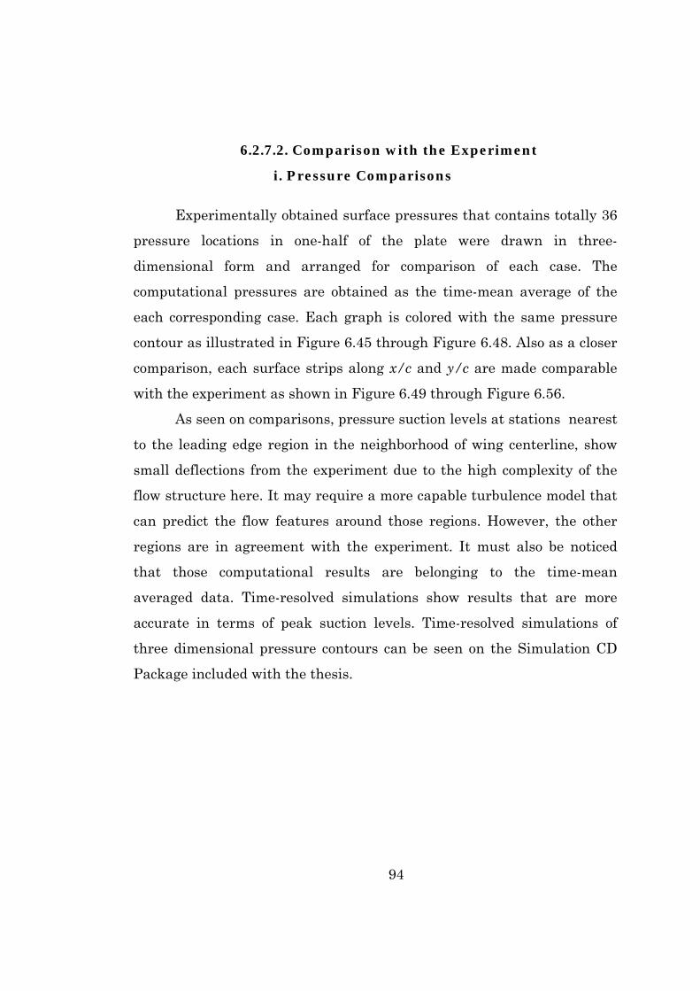
94

6.2.7.2. Comparison with the Experiment

i. Pressure Comparisons

Experimentally obtained surface pressures that contains totally 36

pressure locations in one-half of the plate were drawn in three-

dimensional form and arranged for comparison of each case. The

computational pressures are obtained as the time-mean average of the

each corresponding case. Each graph is colored with the same pressure

contour as illustrated in Figure 6.45 through Figure 6.48. Also as a closer

comparison, each surface strips along x/c and y/c are made comparable

with the experiment as shown in Figure 6.49 through Figure 6.56.

As seen on comparisons, pressure suction levels at stations nearest

to the leading edge region in the neighborhood of wing centerline, show

small deflections from the experiment due to the high complexity of the

flow structure here. It may require a more capable turbulence model that

can predict the flow features around those regions. However, the other

regions are in agreement with the experiment. It must also be noticed

that those computational results are belonging to the time-mean

averaged data. Time-resolved simulations show results that are more

accurate in terms of peak suction levels. Time-resolved simulations of

three dimensional pressure contours can be seen on the Simulation CD

Package included with the thesis.

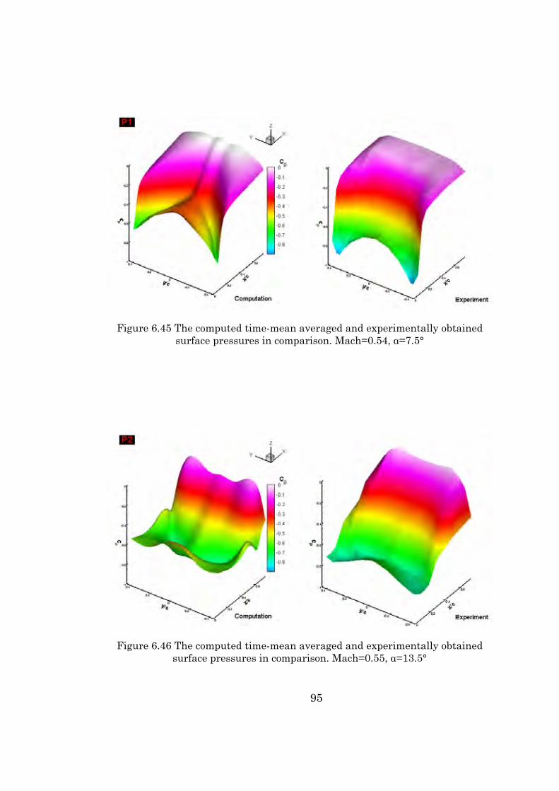
95

Figure 6.45 The computed time-mean averaged and experimentally obtained surface pressures in comparison. Mach=0.54, α=7.5°

Figure 6.46 The computed time-mean averaged and experimentally obtained surface pressures in comparison. Mach=0.55, α=13.5°

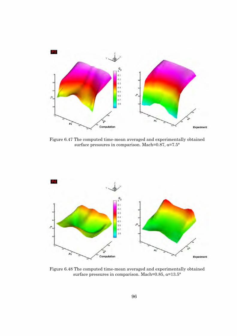
96

Figure 6.47 The computed time-mean averaged and experimentally obtained surface pressures in comparison. Mach=0.87, α=7.5°

Figure 6.48 The computed time-mean averaged and experimentally obtained surface pressures in comparison. Mach=0.85, α=13.5°

97

y/c

Cp

-0.4 -0.2 0 0.2 0.4

-1

-0.8

-0.6

-0.4

-0.2

0

ExperimentExperimentExperimentExperimentExperimentExperimentComputationComputationComputationComputationComputationComputation

y/c

Cp

-0.4 -0.2 0 0.2 0.4

-1

-0.8

-0.6

-0.4

-0.2

0

ExperimentComputation

Case P1 x/c=0.06

y/c

Cp

-0.4 -0.2 0 0.2 0.4

-1

-0.8

-0.6

-0.4

-0.2

0

ExperimentComputation

Case P1 x/c=0.12

y/c

Cp

-0.4 -0.2 0 0.2 0.4

-1

-0.8

-0.6

-0.4

-0.2

0

ExperimentComputation

Case P1 x/c=0.18

y/c

Cp

-0.4 -0.2 0 0.2 0.4

-1

-0.8

-0.6

-0.4

-0.2

0

ExperimentComputation

Case P1 x/c=0.29

y/c

Cp

-0.4 -0.2 0 0.2 0.4

-1

-0.8

-0.6

-0.4

-0.2

0

ExperimentComputation

Case P1 x/c=0.50

y/c

Cp

-0.4 -0.2 0 0.2 0.4

-1

-0.8

-0.6

-0.4

-0.2

0

ExperimentComputation

Case P1 x/c=0.75

Figure 6.49 Comparison of computational and experimental [36] surface pressures along y strips. Case: P1 Mach=0.54, α=7.5°

98

y/c

Cp

-0.4 -0.2 0 0.2 0.4

-1

-0.8

-0.6

-0.4

-0.2

0

ExperimentExperimentExperimentExperimentExperimentExperimentComputationComputationComputationComputationComputationComputation

x/c

Cp

0 0.2 0.4 0.6 0.8 1

-1

-0.8

-0.6

-0.4

-0.2

0

ExperimentComputation

Case P1 y/c=0.00

x/c

Cp

0 0.2 0.4 0.6 0.8 1

-1

-0.8

-0.6

-0.4

-0.2

0

ExperimentComputation

Case P1 y/c=0.13

x/c

Cp

0 0.2 0.4 0.6 0.8 1

-1

-0.8

-0.6

-0.4

-0.2

0

ExperimentComputation

Case P1 y/c=0.32

x/c

Cp

0 0.2 0.4 0.6 0.8 1

-1

-0.8

-0.6

-0.4

-0.2

0

ExperimentComputation

Case P1 y/c=0.24

x/c

Cp

0 0.2 0.4 0.6 0.8 1

-1

-0.8

-0.6

-0.4

-0.2

0

ExperimentComputation

Case P1 y/c=0.38

x/c

Cp

0 0.2 0.4 0.6 0.8 1

-1

-0.8

-0.6

-0.4

-0.2

0

ExperimentComputation

Case P1 y/c=0.44

Figure 6.50 Comparison of computational and experimental [36] surface pressures along x strips. Case: P1 Mach=0.54, α=7.5°

99

y/c

Cp

-0.4 -0.2 0 0.2 0.4

-1

-0.8

-0.6

-0.4

-0.2

0

ExperimentExperimentExperimentExperimentExperimentExperimentComputationComputationComputationComputationComputationComputation

y/c

Cp

-0.4 -0.2 0 0.2 0.4

-1

-0.8

-0.6

-0.4

-0.2

0

ExperimentComputation

Case P2 x/c=0.06

y/c

Cp

-0.4 -0.2 0 0.2 0.4

-1

-0.8

-0.6

-0.4

-0.2

0

ExperimentComputation

Case P2 x/c=0.12

y/c

Cp

-0.4 -0.2 0 0.2 0.4

-1

-0.8

-0.6

-0.4

-0.2

0

ExperimentComputation

Case P2 x/c=0.29

y/c

Cp

-0.4 -0.2 0 0.2 0.4

-0.4

-0.2

ExperimentComputation

Case P2 x/c=0.75

y/c

Cp

-0.4 -0.2 0 0.2 0.4

-1

-0.8

-0.6

-0.4

-0.2

0

ExperimentComputation

Case P2 x/c=0.50

y/c

Cp

-0.4 -0.2 0 0.2 0.4

-1

-0.8

-0.6

-0.4

-0.2

0

ExperimentComputation

Case P2 x/c=0.18

Figure 6.51 Comparison of computational and experimental [36]surface pressures along y strips. Case: P2 Mach=0.55, α=13.5°

100

y/c

Cp

-0.4 -0.2 0 0.2 0.4

-1

-0.8

-0.6

-0.4

-0.2

0

ExperimentExperimentExperimentExperimentExperimentExperimentComputationComputationComputationComputationComputationComputation

x/c

Cp

0 0.2 0.4 0.6 0.8 1

-1

-0.8

-0.6

-0.4

-0.2

0

ExperimentComputation

Case P2 y/c=0.00

x/c

Cp

0 0.2 0.4 0.6 0.8 1

-1

-0.8

-0.6

-0.4

-0.2

0

ExperimentComputation

Case P2 y/c=0.13

x/c

Cp

0 0.2 0.4 0.6 0.8 1

-1

-0.8

-0.6

-0.4

-0.2

0

ExperimentComputation

Case P2 y/c=0.32

x/c

Cp

0 0.2 0.4 0.6 0.8 1

-1

-0.8

-0.6

-0.4

-0.2

0

ExperimentComputation

Case P2 y/c=0.24

x/c

Cp

0 0.2 0.4 0.6 0.8 1

-1

-0.8

-0.6

-0.4

-0.2

0

ExperimentComputation

Case P2 y/c=0.44

x/c

Cp

0 0.2 0.4 0.6 0.8 1

-1

-0.8

-0.6

-0.4

-0.2

0

ExperimentComputation

Case P2 y/c=0.38

Figure 6.52 Comparison of computational and experimental [36] surface pressures along x strips. Case: P2 Mach=0.55, α=13.5°

101

y/c

Cp

-0.4 -0.2 0 0.2 0.4

-1

-0.8

-0.6

-0.4

-0.2

0

ExperimentExperimentExperimentExperimentExperimentExperimentComputationComputationComputationComputationComputationComputation

y/c

Cp

-0.4 -0.2 0 0.2 0.4

-1

-0.8

-0.6

-0.4

-0.2

0

ExperimentComputation

Case P3 x/c=0.06

y/c

Cp

-0.4 -0.2 0 0.2 0.4

-1

-0.8

-0.6

-0.4

-0.2

0

ExperimentComputation

Case P3 x/c=0.12

y/c

Cp

-0.4 -0.2 0 0.2 0.4

-1

-0.8

-0.6

-0.4

-0.2

0

ExperimentComputation

Case P3 x/c=0.18

y/c

Cp

-0.4 -0.2 0 0.2 0.4

-1

-0.8

-0.6

-0.4

-0.2

0

ExperimentComputation

Case P3 x/c=0.29

y/c

Cp

-0.4 -0.2 0 0.2 0.4

-1

-0.8

-0.6

-0.4

-0.2

0

ExperimentComputation

Case P3 x/c=0.75

y/c

Cp

-0.4 -0.2 0 0.2 0.4

-1

-0.8

-0.6

-0.4

-0.2

0

ExperimentComputation

Case P3 x/c=0.50

Figure 6.53 Comparison of computational and experimental [36] surface pressures along y strips. Case: P3 Mach=0.87, α=7.5°

102

y/c

Cp

-0.4 -0.2 0 0.2 0.4

-1

-0.8

-0.6

-0.4

-0.2

0

ExperimentExperimentExperimentExperimentExperimentExperimentComputationComputationComputationComputationComputationComputation

x/c

Cp

0 0.2 0.4 0.6 0.8 1

-1

-0.8

-0.6

-0.4

-0.2

0

ExperimentComputation

Case P3 y/c=0.00

x/c

Cp

0 0.2 0.4 0.6 0.8 1

-1

-0.8

-0.6

-0.4

-0.2

0

ExperimentComputation

Case P3 y/c=0.13

x/c

Cp

0 0.2 0.4 0.6 0.8 1

-1

-0.8

-0.6

-0.4

-0.2

0

ExperimentComputation

Case P3 y/c=0.24

x/c

Cp

0 0.2 0.4 0.6 0.8 1

-1

-0.8

-0.6

-0.4

-0.2

0

ExperimentComputation

Case P3 y/c=0.32

x/c

Cp

0 0.2 0.4 0.6 0.8 1

-1

-0.8

-0.6

-0.4

-0.2

0

ExperimentComputation

Case P3 y/c=0.44

x/c

Cp

0 0.2 0.4 0.6 0.8 1

-1

-0.8

-0.6

-0.4

-0.2

0

ExperimentComputation

Case P3 y/c=0.38

Figure 6.54 Comparison of computational and experimental [36] surface pressures along x strips. Case: P3 Mach=0.87, α=7.5°

103

y/c

Cp

-0.4 -0.2 0 0.2 0.4

-1

-0.8

-0.6

-0.4

-0.2

0

ExperimentExperimentExperimentExperimentExperimentExperimentComputationComputationComputationComputationComputationComputation

y/c

Cp

-0.5 -0.4 -0.3 -0.2 -0.1 0 0.1 0.2 0.3 0.4 0.5

-1

-0.8

-0.6

-0.4

-0.2

0

ExperimentComputation

Case P4 x/c=0.06

y/c

Cp

-0.5 -0.4 -0.3 -0.2 -0.1 0 0.1 0.2 0.3 0.4 0.5

-1

-0.8

-0.6

-0.4

-0.2

0

ExperimentComputation

Case P4 x/c=0.12

y/c

Cp

-0.5 -0.4 -0.3 -0.2 -0.1 0 0.1 0.2 0.3 0.4 0.5

-1

-0.8

-0.6

-0.4

-0.2

0

ExperimentComputation

Case P4 x/c=0.29

y/c

Cp

-0.5 -0.4 -0.3 -0.2 -0.1 0 0.1 0.2 0.3 0.4 0.5

-1

-0.8

-0.6

-0.4

-0.2

0

ExperimentComputation

Case P4 x/c=0.18

y/c

Cp

-0.5 -0.4 -0.3 -0.2 -0.1 0 0.1 0.2 0.3 0.4 0.5

-1

-0.8

-0.6

-0.4

-0.2

0

ExperimentComputation

Case P4 x/c=0.75

y/c

Cp

-0.5 -0.4 -0.3 -0.2 -0.1 0 0.1 0.2 0.3 0.4 0.5

-1

-0.8

-0.6

-0.4

-0.2

0

ExperimentComputation

Case P4 x/c=0.50

Figure 6.55 Comparison of computational and experimental [36] surface pressures along y strips. Case: P4 Mach=0.85, α=13.5°

104

y/c

Cp

-0.4 -0.2 0 0.2 0.4

-1

-0.8

-0.6

-0.4

-0.2

0

ExperimentExperimentExperimentExperimentExperimentExperimentComputationComputationComputationComputationComputationComputation

x/c

Cp

0 0.2 0.4 0.6 0.8 1

-1

-0.8

-0.6

-0.4

-0.2

0

ExperimentComputation

Case P4 y/c=0.00

x/c

Cp

0 0.2 0.4 0.6 0.8 1

-1

-0.8

-0.6

-0.4

-0.2

0

ExperimentComputation

Case P4 y/c=0.13

x/c

Cp

0 0.2 0.4 0.6 0.8 1

-1

-0.8

-0.6

-0.4

-0.2

0

ExperimentComputation

Case P4 y/c=0.32

x/c

Cp

0 0.2 0.4 0.6 0.8 1

-1

-0.8

-0.6

-0.4

-0.2

0

ExperimentComputation

Case P4 y/c=0.24

x/c

Cp

0 0.2 0.4 0.6 0.8 1

-1

-0.8

-0.6

-0.4

-0.2

0

ExperimentComputation

Case P4 y/c=0.44

x/c

Cp

0 0.2 0.4 0.6 0.8 1

-1

-0.8

-0.6

-0.4

-0.2

0

ExperimentComputation

Case P4 y/c=0.38

Figure 6.56 Comparison of computational and experimental [36] surface pressures along x strips. Case: P4 Mach=0.85, α=13.5°

105

ii. Surface Skin-friction Comparisons

The experimentally obtained surface streamlines on the leeward

surface as shown in Figure 6.57 and Figure 6.58 were obtained by using

the oil-flow method in the low speed tunnel at angle of attack of 5° and

angle of attack of 15° ,respectively [39]. In Figure 6.59 and Figure 6.60,

the computationally obtained streamlines are shown for Mach=0.42 at

angle of attack of 5° and angle of attack of 15°, respectively. They are

drawn from the time-mean averaged data obtained by means of averaging

the solution data, stored at the equal time intervals by the computer, over

the one corresponding cycle of computation.

The comparison between computationally and experimentally

obtained streamlines was given in Figure 6.61 and Figure 6.62. The

formation and the size of the leading edge vortices are predicted well. In

addition, the leading edge bubble formation is in good agreement with the

experiment.

Figure 6.63 and Figure 6.64 are deductions from Figure 6.59 and

Figure 6.60 of the corresponding pattern of skin-friction lines,

respectively. The surface streamlines actually represents the traces of the

skin friction lines that describes the structure of the flow separation

around the body. The streamline pattern depicts the various

interconnections between the node, saddle points and the paths of the

separated flow around the leading edge. The streamlines emanating from

the saddle points, called as separatrices, represents the regions of the

flow that separate from one another [26]. It is seen in Figure 6.63 four

spiral nodes, one nodal point of attachment and four saddle points on the

leeward surface. Each of the four saddle points separates the flow from

adjacent pairs of nodes. In Figure 6.64 there are two major and four

minor spiral nodes, four nodal point of attachment and ten saddle points

on the leeward surface. For both patterns, two saddle points situated on

the wing centerline shows the primary and secondary bubbles.

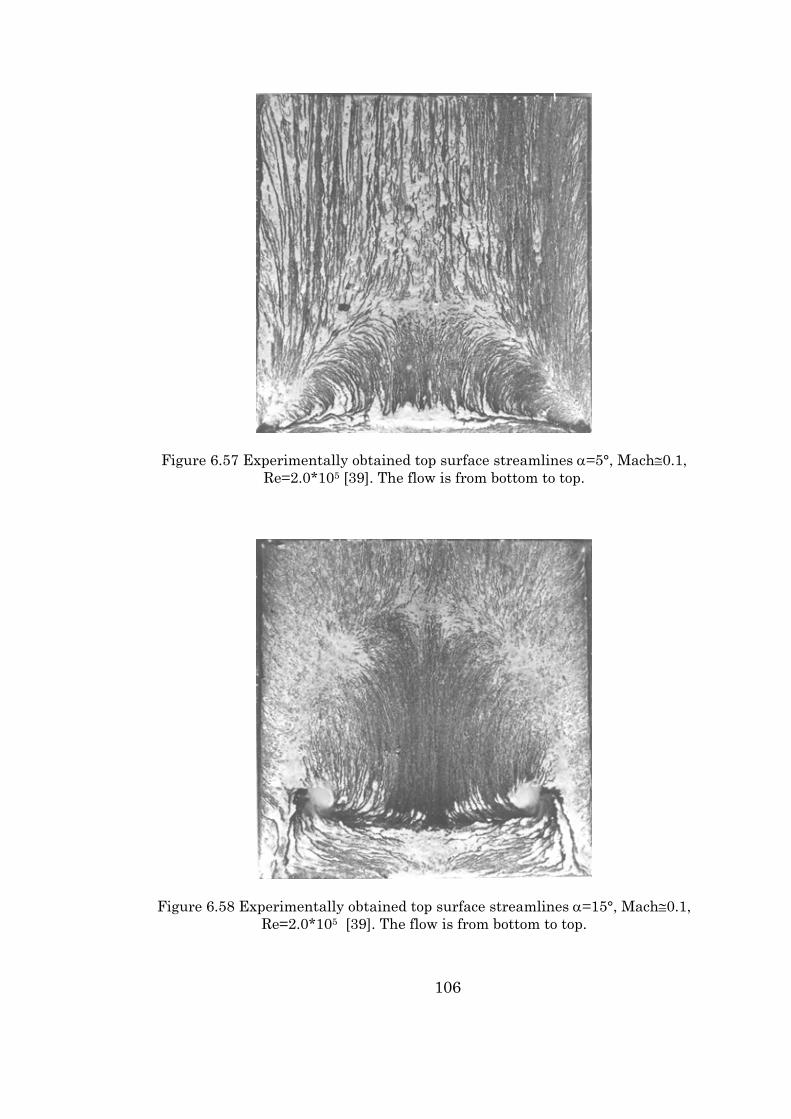
106

Figure 6.57 Experimentally obtained top surface streamlines α=5°, Mach≅0.1, Re=2.0*105 [39]. The flow is from bottom to top.

Figure 6.58 Experimentally obtained top surface streamlines α=15°, Mach≅0.1, Re=2.0*105 [39]. The flow is from bottom to top.

107

Figure 6.59 Computationally obtained top surface streamlines (time-mean averaged). Case: S1 α=5°, Mach = 0.42.

Figure 6.60 Computationally obtained top surface streamlines (time-mean averaged). Case: S2 α=15°, Mach = 0.42.

flow

dir

ectio

n flo

w d

irec

tion

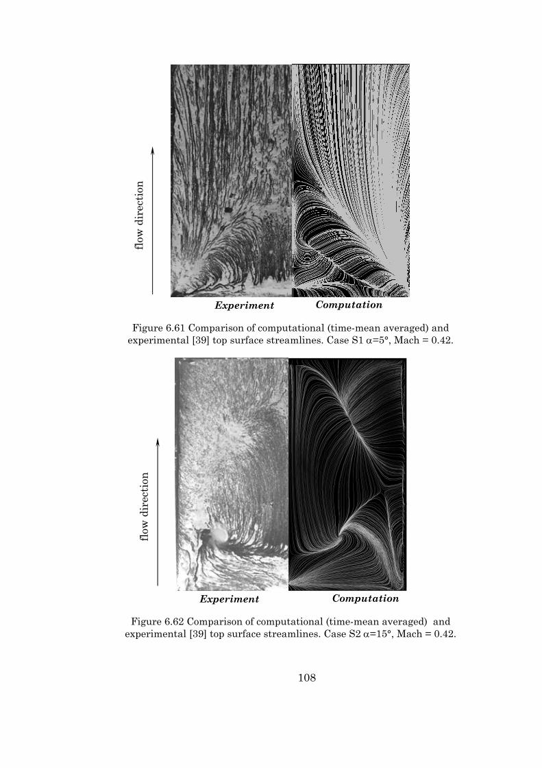
108

Figure 6.61 Comparison of computational (time-mean averaged) and experimental [39] top surface streamlines. Case S1 α=5°, Mach = 0.42.

Figure 6.62 Comparison of computational (time-mean averaged) and experimental [39] top surface streamlines. Case S2 α=15°, Mach = 0.42.

Experiment Computation

Experiment Computation

flow

dir

ectio

n flo

w d

irec

tion

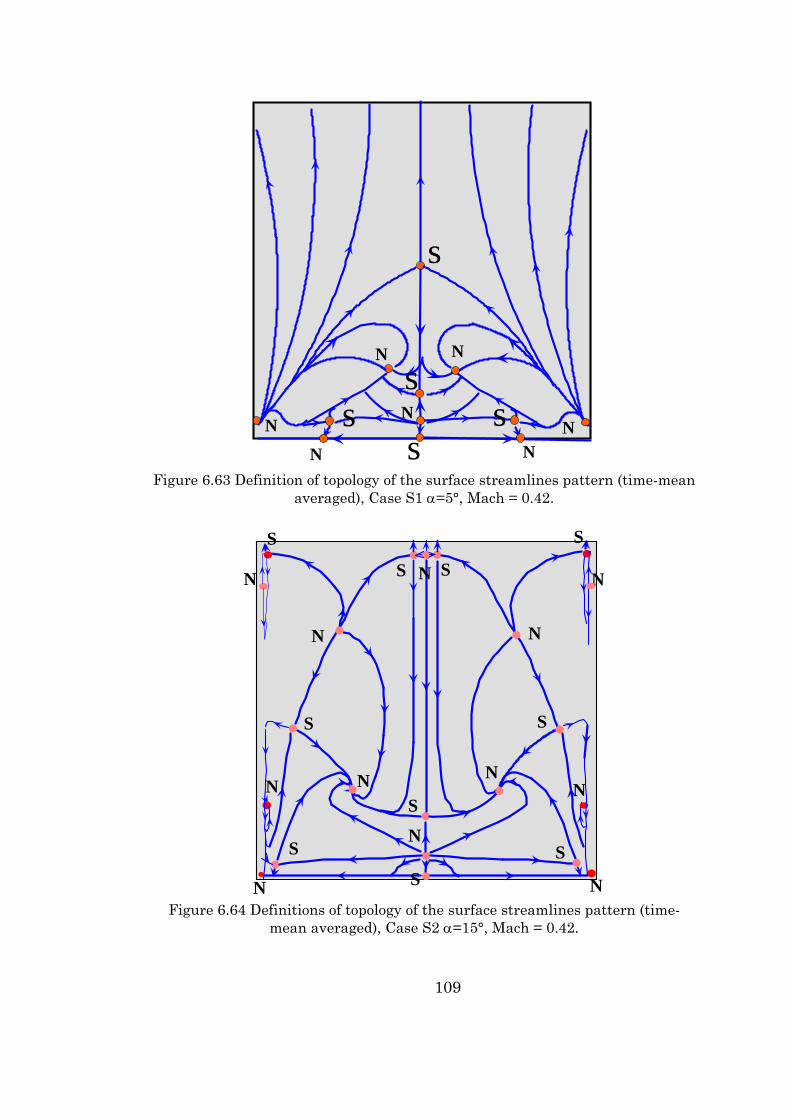
109

s

N

sN

N

ss0

N NN

N

s

Figure 6.63 Definition of topology of the surface streamlines pattern (time-mean

averaged), Case S1 α=5°, Mach = 0.42.

SN N

NS

S

S

N

S

S

N

N

S N

N N

N

S

S

S

N

N

Figure 6.64 Definitions of topology of the surface streamlines pattern (time-

mean averaged), Case S2 α=15°, Mach = 0.42.

110

iii. Force-Moment Comparisons

In Figure 6.65 through Figure 6.70, Normal Force and Pitching

Moment comparisons with the experiment [39] are illustrated. Normal

Force and Pitching Moment values are obtained by the integration of the

surface pressures from the top and the bottom surfaces for each case.

Since the results have the oscillatory behavior, the variables were again

averaged over the corresponding cycle to each case. Hence, each figure

shows the averaged, the maximum and the minimum values of the

Normal Force and the Pitching Moment components over a period of cycle

at the particular angle of attack. It is seen that the differences between

computational and experimental values are the result of differences

between pressure peak suction levels.

S1 - S2

-0,3

-0,2

-0,1

0,0

0,10 2,5 5 7,5 10 12,5 15 17,5 20

angle of attack

CM

o

ExperimentComputation(min&max)Computation(avarage)

Figure 6.65 Comparison of computational and experimental [39] pitching-moment coefficients, Mach = 0.42, Re = 2.0*105. Computational data from

Case’s: S1 and S2.

111

P1 - P2

-0,3

-0,2

-0,1

0,0

0,10 2,5 5 7,5 10 12,5 15 17,5 20

angle of attack

CM

o

ExperimentComputation(min&max)Computation(avarage)

Figure 6.66 Comparison of computational and experimental [39] pitching-moment coefficients, Mach = 0.54-0.55, Re = 2.0*105. Computational data from

Case’s: P1 and P2.

P3 - P4

-0,3

-0,2

-0,1

0,0

0,10 2,5 5 7,5 10 12,5 15 17,5 20

angle of attack

CM

o

ExperimentComputation(min&max)Computation(avarage)

Figure 6.67 Comparison of computational and experimental [39] pitching-moment coefficients, Mach = 0.85-0.87, Re = 2.0*105. Computational data from

Case’s: P3 and P4.

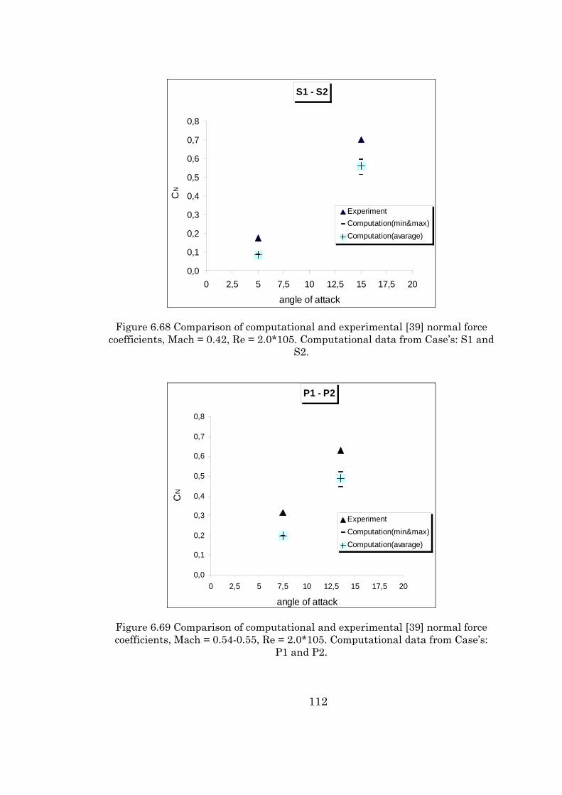
112

S1 - S2

0,0

0,1

0,2

0,3

0,4

0,5

0,6

0,7

0,8

0 2,5 5 7,5 10 12,5 15 17,5 20

angle of attack

CN

ExperimentComputation(min&max)Computation(avarage)

Figure 6.68 Comparison of computational and experimental [39] normal force coefficients, Mach = 0.42, Re = 2.0*105. Computational data from Case’s: S1 and

S2. P1 - P2

0,0

0,1

0,2

0,3

0,4

0,5

0,6

0,7

0,8

0 2,5 5 7,5 10 12,5 15 17,5 20

angle of attack

CN

ExperimentComputation(min&max)Computation(avarage)

Figure 6.69 Comparison of computational and experimental [39] normal force coefficients, Mach = 0.54-0.55, Re = 2.0*105. Computational data from Case’s:

P1 and P2.

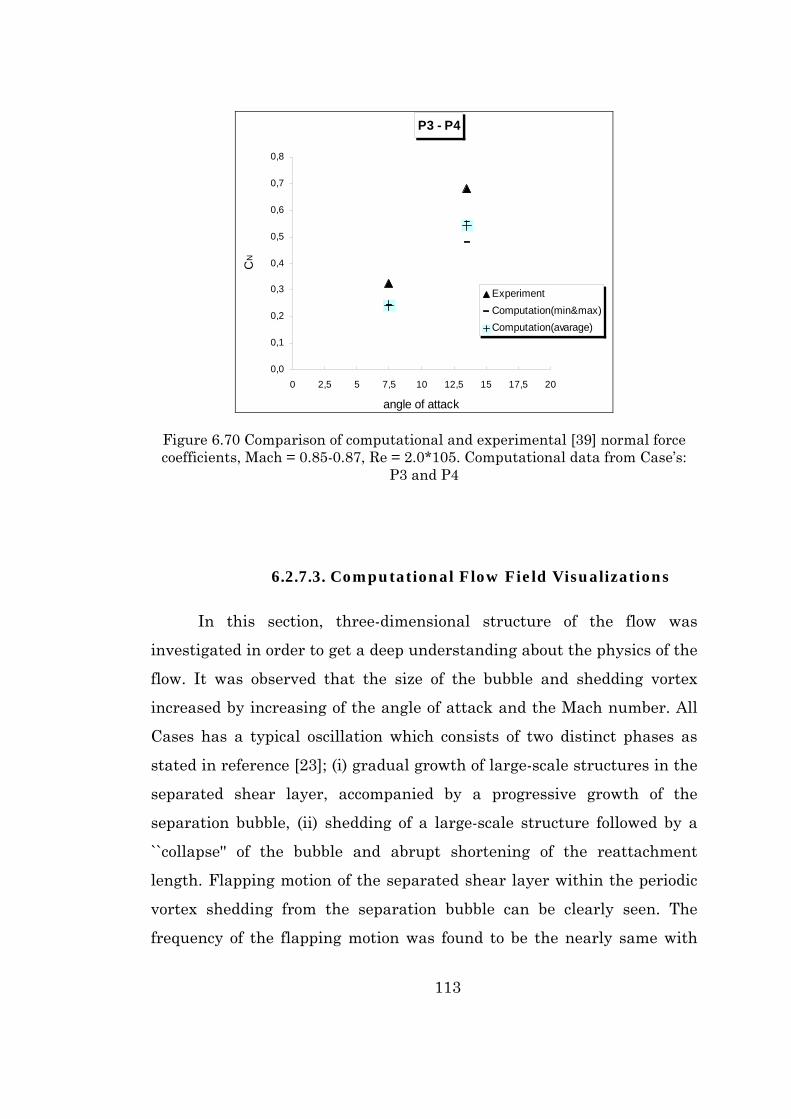
113

P3 - P4

0,0

0,1

0,2

0,3

0,4

0,5

0,6

0,7

0,8

0 2,5 5 7,5 10 12,5 15 17,5 20

angle of attack

CN

ExperimentComputation(min&max)Computation(avarage)

Figure 6.70 Comparison of computational and experimental [39] normal force coefficients, Mach = 0.85-0.87, Re = 2.0*105. Computational data from Case’s:

P3 and P4

6.2.7.3. Computational Flow Field Visualizations

In this section, three-dimensional structure of the flow was

investigated in order to get a deep understanding about the physics of the

flow. It was observed that the size of the bubble and shedding vortex

increased by increasing of the angle of attack and the Mach number. All

Cases has a typical oscillation which consists of two distinct phases as

stated in reference [23]; (i) gradual growth of large-scale structures in the

separated shear layer, accompanied by a progressive growth of the

separation bubble, (ii) shedding of a large-scale structure followed by a

``collapse'' of the bubble and abrupt shortening of the reattachment

length. Flapping motion of the separated shear layer within the periodic

vortex shedding from the separation bubble can be clearly seen. The

frequency of the flapping motion was found to be the nearly same with

114

the vortex shedding frequency as mentioned in Kiya M. et al [6]. In

Figure 6.71, the transient feature of the flow through timeline of S2 Case

is presented in terms of velocity field at the symmetry plane. Time-

resolved simulations obtained by velocity field at the symmetry plane for

each case can be viewed in the Simulation CD Package.

The vortical structure of the flow field around the plate was

illustrated in the Figure 6.72. This figure was extracted from just end of

the timeline of Case S2 in order to show the flow structure clearly. The

predominant structures over the separation bubble are clearly identified

as hairpin (horseshoe) vortices in the reattachment region [23]. The legs

of the horseshoe vortices are inclined with respect to the streamwise

direction. A typical vortex grows in every direction as it is advected

downstream of the reattachment region. Due to the interaction between

the vortical motion of the large-scale structure and the wall, it also tends

to lift away from the wall. This in turn, brings the top end of the

horseshoe vortex into contact with the outer (higher velocity) region,

resulting in further stretching and inclination of the vortex along the flow

direction. Eventually, the central portion breaks down, and only the two

inclined legs remain. In the case of separation bubble formation, there

exist both primary and secondary separation bubbles in that picture. It

verifies the skin-friction topology on the previous chapter that depicts the

secondary separation bubble formation characterized by the saddle point

near the leading edge. Reversed flow sourced by separation vortex occurs

at mid-part and aft part of the side edge of the flat plate.

In that figure, primary vortex actually represents the spanwise

vortices, which are produced by rolling up of the shear layer to form

rectilinear vortex tubes whose axis is aligned with the side edge of the

flat plate. Secondary vortices are also formed under the primary vortex as

seen also on Figure 6.73 which is colored by the total pressure contours. It

shows the transitional streamline plot of the Case S2; α=15°, Mach = 0.42

115

at the spanwise section of the plate, x/c=0.5. For the same Case, a similar

picture that shows the primary and secondary bubble formation at the

symmetry plane, y/c=0.0 is also demonstrated in Figure 6.74. Notice that,

secondary bubble is shown in zoomed view in that figure. Time-resolved

simulations that shows three dimensional flow structures for S1 and S2

Cases were also put in the Simulation CD Package.

116

Figure 6.71 Flow timeline of Case S2 α=15°, Mach = 0.42

t = 0.0 t = 0.90

t = 1.8 t = 2.7

t = 3.6 t = 4.5

t = 5.4 t = 6.3

t = 7.2 t = 8.1

Mach = 0.42 α = 15° f =196 Hz

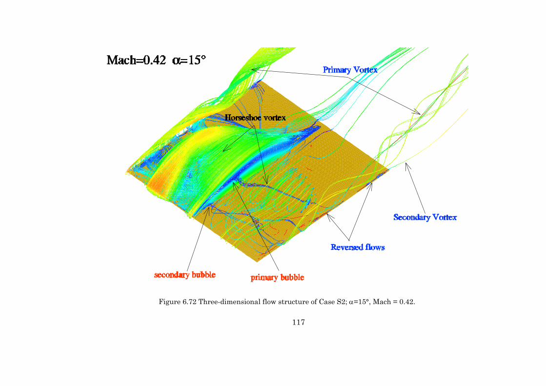
117

Figure 6.72 Three-dimensional flow structure of Case S2; α=15°, Mach = 0.42.

118

Figure 6.73 Primary and secondary vortices at the span wise plane, x/c=0.5.

Figure 6.74 Primary and secondary bubbles at the symmetry plane, y/c=0.0

119

CHAPTER 7

CONCLUSION

Parallel Navier Stokes solutions of an aspect ratio 1.0

rectangular flat plate have been performed at different Mach numbers

and angles of attack to test the validity of the Navier-Stokes code on

the prediction of separated flows, in particular, the ones around the

low aspect ratio wings. The flow separates at the leading edge and

forms the separation bubble. It is dominated by the spanwise vortices

and the rolling-up vortices within the separation bubble. Reynolds

number was of the order of 2.0*105-3.0*105. Two different grid

configurations were adapted namely, the coarse and the fine grids in

order to speed up the convergence of the solutions. For the fine grid

part of the solution, two grid blocks with total of 700,000 points were

used. The initial grid spacing from the surface in the normal direction

was /z c∆ = 0.0001.

There was a strong interference between the separation bubble

and the side edge vortices making the flowfield quite complicated.

Moreover, it was detected that the flow was unsteady and it has

oscillating structure. However, the Baldwin-Lomax turbulence model

modified around the vortical and the wake regions showed acceptable

results. The prediction of the surface streamlines was found to be

accurate to capture the flowfield structure in terms of size and

formation of the primary and the secondary separation bubbles. The

spanwise vortices at the side edges of the flat plate were in good

120

agreement with the experiment, showing both the primary and the

secondary vortices.

It was found that the frequency of the flow, sourced by the

separation bubble, increased with decreasing angle of attack and, its

variation was more rapid for higher Mach numbers. It was also

verified that with the increasing angle of attack, the size and the

intensity of the separation bubble increased and the flow complexity

increased showing more singular points; saddles and nodes on the

surface. In addition, the periodic vortex shedding and the

intermittent nature of the flow field were captured in three-

dimensional time-resolved simulations.

The averaged top surface pressure predictions were in good

agreement except the leading edge region of the wing. This may be

improved by using a more sensitive turbulence model such as Spalart-

Allmaras turbulence model, and by increasing the grid quality in

future.

121

REFERENCES

[1] Russell M. Cummings, James R. Forsytheb, Scott A. Mortonb, Kyle

D. Squiresc, “Computational Challenges in High Angle of Attack

Flow Prediction”, Progress in Aerospace Sciences, 39;369-384, 2003.

[2] Keener ER, Chapman GT., “Similarity in Vortex Asymmetries over

Slender Bodies and Wings”, AIAA, 15;370–2, 1977.

[3] Rom J., “High Angle of Attack Aerodynamics”, New York, Springer,

1992.

[4] Ericsson LE, Reding JP., “Asymmetric Vortex Shedding from

Bodies of Revolution”, Tactical Missile Aerodynamics”, New York,

American Institute of Aeronautics and Astronautics, 1986.

[5] Bertin JJ., “Aerodynamics for Engineers”, Upper Saddle River, NJ:

Prentice-Hall, 2002.

[6] Kiya M., Mochizuki O. and Ishikawa H., “Challenging Issues in

Separated and Complex Turbulent Flows”, Proceedings of the 10th

International Conference on Laser Techniques, 1-13, 2000.

[7] Reece E. Neel, “Advances in Computational Fluid Dynamics:

Turbulent Separated Flows and Transonic Potential Flows”, PhD

Thesis, Virginia Polytechnic Institute and State University.

[8] Alving, A. E., Fernholz, H. H., “Turbulence Measurements around a

Mild Separation Bubble and Downstream of Reattachment”, J.

Fluid Mech. 322, 297– 328, 1996.

122

[9] Kazuhisa Chiba, Shigeru Obayashi, “CFD Visualization of Second

Primary Vortex Structure on a 65-Degree Delta Wing”, 42nd AIAA

Aerospace Sciences Meeting and Exhibit January 5–8, Reno, NV,

AIAA 2004–1231, 2004.

[10] Cherry NJ, Hillier R, “Unsteady Measurements in a Separated and

Reattaching Flow”, J Fluid Mech 144:13–46, 1984.

[11] Kiya M., Sasaki K., “Structure of a Turbulent Separation Bubble”,

J. Fluid Mech 137:83–113, 1983.

[12] Kiya M., Sasaki K., “Structure of Large-Scale Vortices and

Unsteady Reverse Flow in the Reattaching Zone of a Turbulent

Separation Bubble”, J. Fluid Mech 154:463–491, 1985.

[13] Chun S., Sung H.J., “Influence of Unsteady Wake on a Turbulent

Separation Bubble”, Exp. Fluids 32:269–279, 2002.

[14] Hwang K.S., Sung H.J., Hyun J.M., “An Experimental Study of

Largescale Vortices over a Blunt-faced Flat Plate in Pulsating

Flow”, Exp. Fluids 30: 202–213, 2001.

[15] S. Chun, H.J. Sung, “Large-Scale Vortical Structure of Turbulent

Separation Bubble Affected by Unsteady Wake”, Experiments in

Fluids 34, 572–584, 2003.

[16] Carl H¨aggmark, “Investigations of Disturbances Developing in a

Laminar Separation Bubble Flow”, Technical Reports from Royal

Institute of Technology Department of Mechanics S-100 44

Stockholm, Sweden, March 2000.

[17] Kiya M., Ishikawa H., “Coherent Structures and Large Low-

Frequency Irregularity in Free Turbulent Shear Flows Educed by

Wavelet Transform and Proper Orthogonal Decomposition”,

123

Proceedings of 2nd China-Japan Workshop on Turbulent Flows

(Ed. Qing-Ding Wei), 8-22, State Key Laboratory for Turbulence

Research, Peking University, Peking, 1997.

[18] Hourigan K., Thompson M. C. and Tan B. T., “Self-Sustained

Oscillations in Flows around Long Blunt Plates”, Journal of Fluids

and Structures, 15;387-398, 2001.

[19] Sigurdson L.W., “The Structure and Control of Turbulent

Reattaching Flow”, Journal of Fluid Mechanics, 248;267-296, 1995.

[20] Nakamura Y., Nakashima M., “Vortex Excitation of Prisms with

Elongated Rectangular H and Cross Sections”, Journal of Fluid

Mechanics, 163;149-169, 1986.

[21] Djilali N., Gartshore I.S., “Turbulent Flow around a Bluff

Rectangular Plate”, Part I: Experimental investigation, ASME J.

Fluids Eng., 113;51-59. 1991

[22] Saathoff P.J., Melbourne W.H., “Effects of Free Stream Turbulence

on Surface Pressure Fluctuations in a Separation Bubble”, J. Fluid

Mech., 337;1-24, 1997.

[23] Suksangpanomrung N., Djilali and Moinat P., “Large-Eddy

Simulation of Separated Flow over a Bluff Rectangular Plate”,

France International Journal of Heat and Fluid Flow, 21;655-63,

2000.

[24] Yates L. A., Chapman G. T., “Streamlines, Vorticity Lines and

Vortices around Three Dimensional Bodies”, AIAA Journal,

30(7);1819-1826, July 1992.

[25] Simpson R. L., “Aspects of Turbulent Boundary-Layer Separation”,

Progress in Aerospace Sciences, 32;457-521, 1996.

124

[26] Tobak M., Peake D.J, “Topology of Three-Dimensional Separated

Flows “, Annual Review of Fluid Mechanics, Vol. 14, pp. 61-85, 1982

[27] Lighthill, M.J., “Attachment and Separation in Three-Dimensional

Flow,” Laminar Boundary Layers, Vol. 26, pp. 72-82, 1963.

[28] Wickens R.H., “The Vortex Wake and Aerodynamic Load

Distribution of Slender Rectangular Plates( The Effects of a 20°

Bend at Mid-Chord)”, National Research Council of Canada Aero

Report LR-458, July 1966.

[29] Fink M.P., Lastinger J.L., “Aerodynamic Characteristics of Low-

Aspect Ratio Wings in Close Proximity to the Ground”, NACA TN

D-926, 1961.

[30] Peake D.J., Tobak M., “Three Dimensional Flows about Simple

Components at Angle of Attack”, AGARD LS-121, 1982.

[31] AGARD LS-98, Missile Aerodynamics, 1979.

[32] AGARD LS-121, High Angle of Attack Aerodynamics, 1982.

[33] AGARD CP-494, Vortex Flow Aerodynamics, 1991.

[34] AGARD CP-497, Maneuvering Aerodynamics, 1991.

[35] AGARD R-776, Special Coarse on Aircraft Dynamics at High

Angles of Attack: Experiments and Modelling, 1992.

[36] Stahl W. H., “Aerodynamics of Low Aspect Ratio Wings”, AGARD

LS-98, Missile Aerodynamics, 1979.

[37] Winter H., “Strömungsvorgange an Platten und profilierten

Körpern bei kleinen Spannweiten”, Forsch. Ing. -Wes., Vol. 6, , pp.

40-50, 1937.

125

[38] Van Westerhoven P., Wedemeyer E., Wendt J. F., “Low Aspect

Ratio Rectangular Wings at High Incidences”, Paper presented at

the AGARD Symposium on Missile Aerodynamics, Trondheim,

Norway, September 20-22, 1982.

[39] Kavsaoğlu M. Ş, “Flow Around Low Aspect Ratio Rectangular Flat

Plates Including Compressibility”, von Karman Institute For Fluid

Dynamics, VKI-PR 1982-15, June 1982.

[40] Reece E. Neel, “Advances in Computational Fluid Dynamics:

Turbulent Separated Flows and Transonic Potential Flows”, PhD

Thesis, Virginia Polytechnic Institute And State University.

[41] Simpson R. L., “Two-Dimensional Turbulent Separated Flow”,

AGARDograph 287, vol. 1, 1985.

[42] Simpson R. L., “Turbulent Boundary-Layer Separation”, Annual

Review of Fluid Mechanics, vol. 21, pp. 205-234, 1989.

[43] Rockwell, D, “Active Control of Globally-Unstable Separated

Flows”, In proceedings of the ASME Symposium on Unsteady

Flows, 3-9 June, Toronto, Canada 1990.

[44] Hijikata K., Suzuki Y. and Iwana K., “Flow Visualization by

Velocity–Pressure Cross Correlation”, J. Fluid Eng., 118;486–493,

1996.

[45] Johansson A.V., Her J.Y. and Haritonidis J.H., “On the Generation

of High-Amplitude Wall-Pressure Peaks in Turbulent Separation

Bubble”, J. Fluid Mech., 175:119–142, 1987.

[46] Chun S., Sung H.J., “Influence of Unsteady Wake on a Turbulent

Separation Bubble”, Exp. Fluids 32:269–279, 2002.

126

[47] Ekaterinaris J. A., Schiff L. B., “Numerical Prediction of Vortical

Flow over Slender Delta Wings”, Journal of Aircraft, Vol. 30, No. 6,

, pp. 935–942, 1993.

[48] Murayama M., Nakahashi K., Obayashi S., and Kato T.,

“Numerical Simulation of Vortical Flows Using Vorticity

Confinement Coupled with Unstructured Adaptive Grid

Refinement”, Computational Fluid Dynamics Journal, Vol. 10, No.

1, pp. 28–36, 2001.

[49] Luckring J.M., “Reynolds Number and Leading-Edge Bluntness

Effects on a 65° Delta Wing”, AIAA Paper 2002-0419, 2002.

[50] Chu J., Luckring J.M., “Experimental Surface Pressure Data

Obtained on 65° Delta Wing across Reynolds Number and Mach

Number Ranges”, NASA TM-4645, Feb 1996.

[51] Djilali N., Gartshore I.S., “Turbulent Flow around a Bluff

Rectangular Plate”, Part II: Numerical Predictions, ASME J. Fluids

Eng., 113;60-67, 1991.

[52] Nakamura Y., Ohya Y. and Tsuruta H., “Experiments on Vortex

Shedding at Plates with Square Leading and Trailing Edges”,

Journal of Fluid Mechanics, 222;437-447, 1991.

[53] Naudascher E., Wang Y., “Flow-Induced Vibration of Prismatic

Bodies and Grids of Prisms”, Journal of Fluids and Structures, 7

;341-373, 1993.

[54] Hourigan K., Mills R., Thompson M.C., Sheridan J., Dilin P. and

Welsh M.C., “Base Pressure Coefficients for Flows around

Rectangular Plates”, Journal of Wind Engineering and Industrial

Aerodynamics, 49;311-318, 1993.

127

[55] Mills R., Sheridan J., Hourigan K. and Welsh M.C., “The

Mechanism Controlling Vortex Shedding from Rectangular Bluff

Bodies”, In Proceedings of the 12th Australasian Fluid Mechanics

Conference (Ed. R. W. Bilger), 227-230, 10-15 December, Sydney,

Australia 1995.

[56] Mills R.H., “Vortex Interaction in Flows over Blunt Bodies”, Ph.D.

Dissertation, Department of Mechanical Engineering, Monash

University, Melbourne, Australia 1998.

[57] Tan B.T., Thompson M.C. and Hourigan K., “Flow around Long

Rectangular Plates under Cross-Flow Perturbations”, International

Journal Of Fluid, Article 1, 1998.

[58] Sadatoshi Taneda, “Instability Waves in the Shear Layer over a

Separation Bubble”, Fluid Dynamics Research, 27;335-351, 2000.

[59] Alving A.E., Fernholz H.H., “Turbulence Measurements around a

Mild Separation Bubble and Downstream of Reattachment”, J.

Fluid Mech, 322;297-328, 1996.

[60] Thomas James L., Krist Sherrie T. and Anderson W.Kyle, “Navier-

Stokes Computations of Vortical Flows over Low_Aspect-Ratio

Wings”, AIAA Journal, VOL.28, No.2, February 1990.

[61] Kevin Waclawicz, “The Relationship between Crossflow Velocity

and Off-the-Surface Streamtrace Topology for a Moderately Swept

Wing at Transonic Mach Numbers”, MSc Thesis, Virginia

Polytechnic Institute and State University.

[62] Delery Jean M., “Robert Legendre and Henri Werle, “Toward the

Elucidation of Three- Dimensional Separation”, Annual Review of

Fluid Mechanics, Vol. 33;129-154, 2001.

128

[63] Legendre R., “Separation de L’ecoulement Laminaire

Tridimentsionnel”, La Recherche Aeronautique, 54;,3-8, 1956.

[64] Chapman Gary T., “Topological Classification of Flow Separation”,

AIAA Paper 86-0485, 1986.

[65] Wang K.C., “Separation of Three-Dimensional Flow”, Reviews in

Viscous Flow, 341-414, 22 June 1976

[66] Cipolla K.M., Rockwell D., “Instantaneous Crossflow Topology on a

Delta Wing in Presence of Vortex Breakdown”, Journal of Aircraft,

Vol.35, 218-222, March 1998.

[67] Hunt J.C., Abell C.J, Peterka J.A. and Woo H., “Kinematical

Studies of the Flows Around Free or Surface-Mounted Obstacles;

Applying Topology to Flow Visualization”, Journal of Fluid

Mechanics, 179-200, 1986

[68] Chan W.M., Steger J.L., “Enhancements of a Three Dimensional

Hyperbolic Grid Generation Scheme”, Applied Mathematics and

Computation, Vol. 51, No.1, , 181-205, 431-438, 1992.

[69] Steger J.L., Rizk Y.M., “Generation of Three-Dimensional Body-

Fitted Coordinates using Hyperbolic Partial Differential

Equations”, NASA TM 86753, NASA-Ames Research Center,

Motted Field, California, 1985.

[70] Tai C.H.,. Chiang D.C and Su Y. P., “Three Dimensional Hyperbolic

Grid Generation with Inherent Dissipation and Laplacian

Smoothing”, AIAA Journal, Vol. 34, No. 9, Sept. 1996.

[71] Zwan R.J., “Lann Wing, Pitching Oscillation”, AGARD Report No:

702, Compendium of Unsteady Aerodynamics , Addendum No:1,

1985.

129

[72] Baldwin B.S., Lomax H., “Thin Layer Approximation and Algebraic

Model for Separated Turbulent Flows”, AIAA 16th Aerospace

Meeting, Huntsville, Alabama, January, 1978.

[73] Degani D., Schiff L., “Computation of Turbulent Supersonic Flows

Bodies having Crossflow Separation”, Journal of Computational

Physics, Vol 66, 173-196, 1986.

[74] User’s Guide, NPARC Flow Simulator Version 3.0.

[75] Karlsruhe Parallel Program for Aerodynamics (KAPPA)

Dokumentation Magagnato, The Institute for Fluid Mechanics,

University of Karlsruhe, 1996.

[76] Durmuş G., “Three Dimensional Hyperbolic Grid Generation”, MS

Thesis, Middle East Technical University, Department of

Aeronautical Engineering, September 1998.

[77] Schetz J. A., “Boundary Layer Analysis”, Prentice Hall, 1993.

[78] Roberts G.O., “Computational Meshes for Boundary Layer

Problems”, Proceedings of the Second International Conference on

Numerical Methods in Fluid Dynamics, Lecture Notes in Physics,

Vol. 8, Springer-Verlag, New York, 171-177, 1971.

[79] Coles D.E., Hirst E.A. eds., “Computation of Turbulent Boundary

Layers -1968”, Proceedings of the AFOSR-IFP-Stanford Conference,

Vol. II, Stanford University, 1968.

[80] Daily J.W., Harleman D.R.F., “Fluid Dynamics”, Addison-Wesley,

Reading, Massachusetts 1966.

[81] White F.M., “Viscous Fluid Flow”, McGraw-Hill Book Company,

New York 1974.

130

[82] Şen T. S., “Development of a Three Dimensional Multiblock Parallel

Navier Stokes Solver”, PhD Thesis, Middle East Technical University,

Department of Aeronautical Engineering, November 2001.

[83] Beam R.W., Warming R.F., “An Implicit Finite Difference Algorithm for

Hypersonic Systems in Conservation Form”, Journal of Computational

Physics, Vol. 23, 87-110, 1976

[84] Fujii K., “Practical Applications of New LU-ADI Scheme for the Three

Dimensional Navier-Stokes Computation of Transonic Viscous Flows”,

AIAA 24th Aerospace Sciences Meeting, Reno, Nevada, January 1986.

131

CURRICULUM VITAE

PERSONAL INFORMATION Surname, Name : Durmuş, Gökhan Nationality : Turkish (TC) Date of Birth : 13 October 1972 Place of Birth : Ankara Marital Status : Single Phone : +90 312 344 48 83 Email : gdurmus@anadolu.edu.tr EDUCATION

Degree PhD

Institution METU Aerospace Engineering

Year of Graduation 2004

MS METU Aerospace Engineering 1998 BS METU Aerospace Engineering 1995

WORK EXPERIENCE

Year Place Enrollment

1996- Present Anadolu University Civil Aviation School, Eskişehir Research Assistant

FOREIGN LANGUAGES Advanced English, Beginner German PUBLICATIONS 1. Durmuş G., Kavsaoğlu M. Ş., “Control of Hyperbolic Grids”, Aia `98 –

Proceedings of the 2nd Ankara International Aerospace Conference, 9-11 September 1998, Middle East Technical University, Ankara, Turkey, pp. 120-124.

2. Durmuş G., Kavsaoğlu M. Ş., “Marching Distance Functions for Smooth

Control of Hyperbolic Grids”, Aiaa Journal, Vol 38, No: 10, October 2000.

132

3. Durmuş G., Kavsaoğlu M. Ş., “Multi Block Navier Stokes Solutions of Low

Aspect Ratio Rectangular Flat Wings in Compressible Flow”, In Proceedings of The 23rd International Congress of Aeronautical Sciences, Toronto, Canada, 8-13 September, 2002.

4. Durmuş G., Kavsaoğlu M. Ş., “Düz Levha Üzerindeki Laminer Sınır Tabaka

Akımının Navier Stokes Analizinde Çözüm Ağı Etkileri” Kayseri 5. Havacılık Sempozyumu, Erciyes University, Civil Aviation School, 13-14 May 2004, Kayseri, Turkey.

5. Durmuş G., Kavsaoğlu M. Ş, Kaynak Ü., “Parallel Solution of Low Aspect

Ratio Rectangular Flat Wings in Compressible Flow”, 43rd AIAA Aerospace Sciences Meeting and Exhibit, 10 - 13 Jan 2005, Reno, Nevada.( to be published)