Parallel Peeling Algorithms

Jiayang Jiang ∗ Michael Mitzenmacher† Justin Thaler ‡

Abstract

The analysis of several algorithms and data structures can be framed as a peeling process on a ran-dom hypergraph: vertices with degree less than k are removed until there are no vertices of degree lessthan k left. The remaining hypergraph is known as the k-core. In this paper, we analyze parallel peelingprocesses, where in each round, all vertices of degree less than k are removed. It is known that, below aspecific edge density threshold, the k-core is empty with high probability. We show that, with high prob-ability, below this threshold, only 1

log((k−1)(r−1)) log logn+O(1) rounds of peeling are needed to obtainthe empty k-core for r-uniform hypergraphs; this bound is tight up to an additive constant. Interestingly,we show that above this threshold, Ω(logn) rounds of peeling are required to find the non-empty k-core.Since most algorithms and data structures aim to peel to an empty k-core, this asymmetry appears for-tunate. We verify the theoretical results both with simulation and with a parallel implementation usinggraphics processing units (GPUs). Our implementation provides insights into how to structure parallelpeeling algorithms for efficiency in practice.

1 Introduction

Consider the following peeling process: starting with a random hypergraph, vertices with degree less than kare repeatedly removed, together with their incident edges. (We use edges instead of hyperedges throughoutthe paper, as the context is clear.) This yields what is called the k-core of the hypergraph, which is themaximal subgraph where each vertex has degree at least k. It is known that the k-core is uniquely definedand does not depend on the order vertices are removed. The greedy peeling process produces sequentialalgorithms with very fast running times, generally linear in the size of the graph. Because of its simplicityand efficiency, peeling-based approaches appear especially useful for problems involving large data sets.Indeed, this process, and variations on it, have found applications in low-density parity-check codes [14, 17],hash-based sketches [4, 9], satisfiability of random boolean formulae [3, 19], and cuckoo hashing [20].Frequently, the question in these settings is whether or not the k-core is empty. As we discuss further below,it is known that below a specific edge density threshold c∗k,r, the k-core is empty with high probability. Thisasymptotic result in fact accurately predicts practical performance quite well.

In this paper, we focus on expanding the applicability of peeling processes by examining the use ofparallelism in conjunction with peeling. Peeling seems particularly amenable to parallel processing via thefollowing simple round-based algorithm: in each round, all vertices of degree less than k and their adjacent

∗Harvard University, School of Engineering and Applied Sciences. Supported by NSF grants CCF-0915922 and IIS-0964473.†Harvard University, School of Engineering and Applied Sciences. Supported in part by NSF grants CCF-0915922, IIS-

0964473, and CNS-1011840.‡Simons Institute for the Theory of Computing at UC Berkeley. The majority of this work was performed while the author was

a graduate student at Harvard University, School of Engineering and Applied Sciences. Supported by an NSF Graduate ResearchFellowship, NSF grant CCF-0915922, and a Simons Research Fellowship.

1

edges are removed in parallel from the graph. The major question we study is: how many rounds arenecessary before peeling is complete?

We show that, with high probability, when the edge density is a constant strictly below the threshold c∗k,r,only 1

log((k−1)(r−1)) log logn+O(1) rounds of peeling are needed for r-uniform hypergraphs. (The hiddenconstant in the O(1) term depends on the size of the “gap” between the edge density and the thresholddensity. We more precisely characterize this dependence later.) Specifically, we show that the fraction ofvertices that remain in each round decreases doubly exponentially, in a manner similar in spirit to existinganalyses of “balanced allocations” load-balancing problems [2, 15]. Interestingly, we show in contrast thatat edge densities above the threshold, with high probability Ω(logn) rounds of peeling are required to findthe non-empty k-core. Since most algorithms and data structures that use peeling aim for an empty k-core,the fact that empty k-cores are faster to find in parallel than non-empty ones appears particularly fortuitous.

We then consider some of the details in implementation, focusing on the algorithmic example of In-vertible Bloom Lookup Tables (IBLTs) [9]. An IBLT stores a set of keys, with each key being hashed intor cells in a table, and all keys in a cell XORed together. The IBLT defines a random hypergraph, wherekeys correspond to edges, and cells to vertices. As we describe later, recovering the set of keys from theIBLT corresponds to peeling on the associated hypergraph. Applications of IBLTs are further discussed in[9]; they can be used, for example, for sparse recovery [9], simple low-density parity-check codes [17], andefficient set reconciliation across communication links [7]. Our implementation demonstrates that our par-allel peeling algorithm yields concrete speedups, and provides insights into how to structure parallel peelingalgorithms for efficiency in practice.

Our results are closely related to work of Achlioptas and Molloy [1]. With different motivations than ourown, they show that at most O(logn) rounds of peeling are needed to find the (possibly non-empty) k-coreboth above and below the threshold edge density c∗k,r. Our O(log logn) upper bound below the threshold isan exponential improvement on their O(logn) bound, while our Ω(logn) lower bound above the thresholddemonstrates the tightness of their upper bound in this regime. Perhaps surprisingly, we cannot find otheranalyses of parallel peeling in the literature, although early work by Karp, Luby, and Meyer auf der Heide onPRAM simulation uses an algorithm similar to peeling to obtain O(log logn) bounds for load balancing [11],and we use other load balancing arguments [2, 21] for inspiration. We also rely heavily on the frameworkestablished by Molloy [19] for analyzing the k-core of random hypergraphs.

Subsequent to our work, Gao [8] has provided an alternative proof of an O(log logn) upper bound onthe number of rounds required to peel to an empty core when the edge density is below the threshold c∗k,r.Her proof, short and elegant, obtains a leading constant of 1

log(k(r−1)/r) , larger than the constant 1log((k−1)(r−1))

obtained through our more detailed analysis.

Paper Outline. Section 3 characterizes the round complexity of the peeling process when the edge density isa constant strictly below the threshold c∗k,r, showing that the number of rounds required is 1

log((k−1)(r−1)) log logn+O(1). Section 4 shows that when the edge density is a constant strictly above the threshold c∗k,r, the num-ber of rounds required is Ω(logn). Section 5 presents simulation results demonstrating that our theoreticalanalysis closely matches the empirical evolution of the peeling process. Section 6 describes our GPU-basedIBLT implementation. Our IBLT implementation must deal with a fundamental issue that is inherent toany implementation of a parallel peeling algorithm, regardless of the application domain: the need to avoidpeeling the same item multiple times. Consequently, the peeling process used in our IBLT implementationdiffers slightly from the one analyzed in Sections 3 and 4. In Appendix B we formally analyze this variantof the parallel peeling process, demonstrating that it terminates significantly faster than might be expected.

As discussed above, the hidden constant in the additive O(1) term in the upper bound of Section 3depends on the distance between the edge density and the threshold density c∗k,r; we refer to this distance as

2

ν . Section 7 extends the analysis of Section 3 to precisely characterize this dependence, demonstrating thatthere is an additive Θ(1/

√ν) term in the number of rounds required. Section 8 concludes.

2 Preliminaries

For constants r ≥ 2 and c, let Grn,cn denote a random hypergraph1 with n vertices and cn edges, where each

edge consists of r distinct vertices. Such hypergraphs are called r-uniform, and we refer to c as the edgedensity of Gr

n,cn. Previous analyses of random hypergraphs have determined the threshold values c∗k,r suchthat when c < c∗k,r, the k-core is empty with probability 1− o(1), and when c > c∗k,r, the k-core is non-empty with probability 1−o(1). Here and throughout this paper, k,r ≥ 2, but the special (and already wellunderstood) case of k = r = 2 is excluded from consideration. From [19], the formula for c∗k,r is given by

c∗k,r = minx>0

x

r(1− e−x ∑k−2j=0

x j

j! )r−1

. (2.1)

For example, we find that c∗2,3 ≈ 0.818, c∗2,4 ≈ 0.772 and c∗3,3 ≈ 1.553.

3 Below the Threshold

In this section, we characterize the number of rounds required by the peeling process when the edge densityc is a constant strictly below the threshold density c∗k,r. Recall that this peeling process repeatedly removesvertices with degree less than k, together with their incident edges. We prove the following theorem.

Theorem 1. Let k,r ≥ 2 with k + r ≥ 5, and let c be a constant. With probability 1− o(1), the parallelpeeling process for the k-core in a random hypergraph Gr

n,cn with edge density c and r-ary edges terminatesafter 1

log((k−1)(r−1)) log logn+O(1) rounds when c < c∗k,r.

Theorem 1 is tight up to an additive constant.

Theorem 2. Let k,r ≥ 2 with k + r ≥ 5, and let c be a constant. With probability 1− o(1), the parallelpeeling process for the k-core in a random hypergraph Gr

n,cn with edge density c and r-ary edges requires1

log((k−1)(r−1)) log logn−O(1) rounds to terminate when c < c∗k,r.

In proving Theorems 1 and 2, we begin in Section 3.1 with a high-level overview of our argument, beforepresenting full details of the proof in Section 3.2.

3.1 The High-Level Argument

The neighborhood of a node v in a random r-uniform hypergraph can be accurately modeled as a branchingprocess, with a random number of edges adjacent to this vertex, and similarly a random number of edgesadjacent to each of those vertices, and so on. For intuition, we assume this branching process yields a tree,and further that the number of adjacent edges is distributed according to a discrete Poisson distribution withmean rc. These assumptions are sufficiently accurate for our analysis, as we later prove. (This approach isstandard; see e.g. [6, 19] for similar arguments.)

The intuition for the main result comes from considering the (tree) neighborhood of v, and applying thefollowing algorithm: for 1≤ i≤ t−1, in round i, look at all the vertices at distance t− i and delete a vertex

1When r = 2 we have a graph, but we may use hypergraph when speaking generally.

3

if it has fewer than k− 1 child edges. Finally, in round t, v is deleted if it has degree less than k. Vertex vsurvives after t rounds of peeling if and only if it survives after t rounds of this algorithm.

In what follows, we denote the probability that v survives after t rounds in this model by λt , and theprobability a vertex u at distance t− i from v survives i rounds by ρi.

Here ρ0 = 1. In this idealized setting, the following relationships hold:ρi = Pr(Poisson(ρr−1

i−1 rc)≥ k−1),

and similarly

λi = Pr(Poisson(ρr−1i−1 rc)≥ k). (3.1)

The recursion for ρi arises as follows: each node u has a Poisson distributed number of descendant edgeswith mean rc, and each edge has r−1 additional vertices that each survive i−1 rounds with probability ρi−1.By the splitting property of Poisson distributions [16, Chapter 5], the number of surviving descendant edgesof u is Poisson distributed with mean ρ

r−1i−1 rc, and this must be at least k− 1 for u to itself survive the ith

round.We use βi to represent the expected number of surviving descendant edges after i−1 rounds:

βi = ρr−1i−1 rc.

Then,

ρi = 1− e−βik−2

∑j=0

βij

j!, (3.2)

λi = 1− e−βik−1

∑j=0

βij

j!, (3.3)

βi+1 =

[1− e−βi

k−2

∑j=0

βij

j!

]r−1

rc. (3.4)

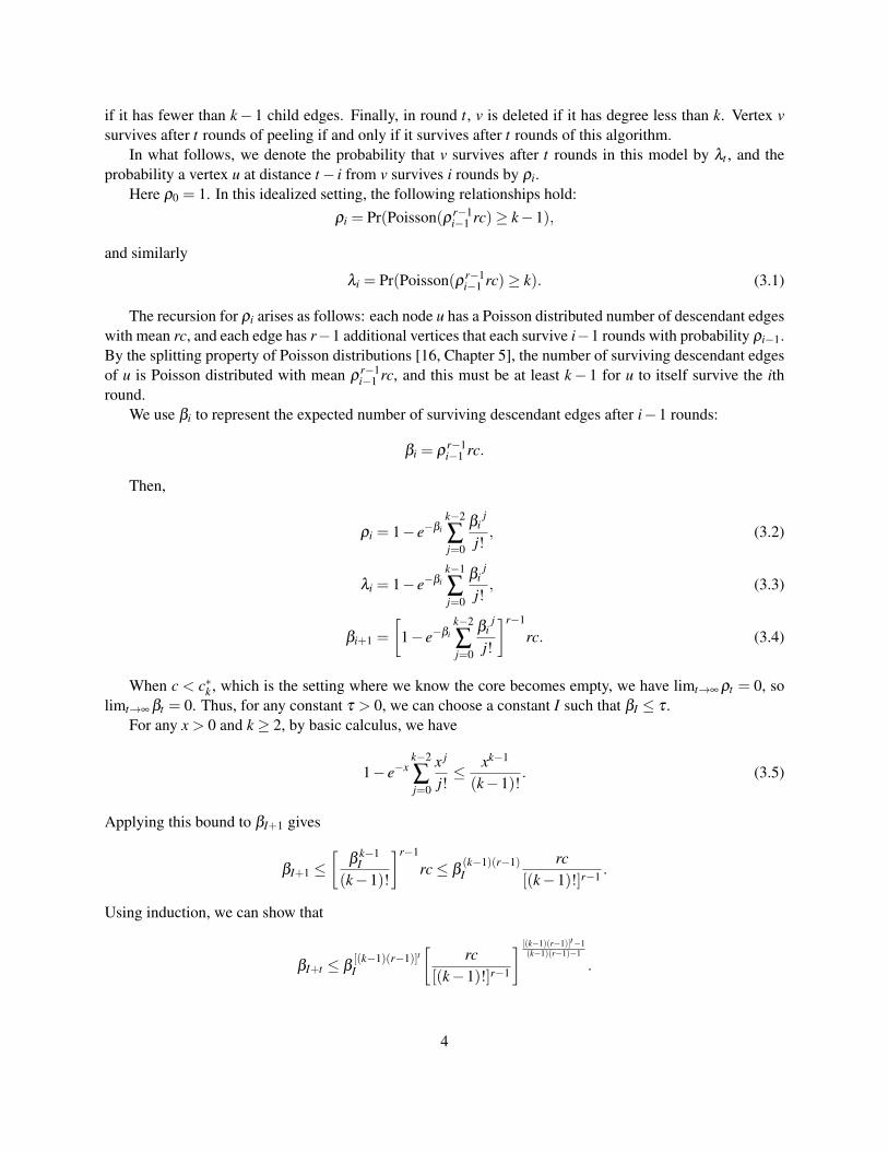
When c < c∗k , which is the setting where we know the core becomes empty, we have limt→∞ ρt = 0, solimt→∞ βt = 0. Thus, for any constant τ > 0, we can choose a constant I such that βI ≤ τ .

For any x > 0 and k ≥ 2, by basic calculus, we have

1− e−xk−2

∑j=0

x j

j!≤ xk−1

(k−1)!. (3.5)

Applying this bound to βI+1 gives

βI+1 ≤[

βk−1I

(k−1)!

]r−1

rc≤ β(k−1)(r−1)I

rc[(k−1)!]r−1 .

Using induction, we can show that

βI+t ≤ β[(k−1)(r−1)]tI

[rc

[(k−1)!]r−1

] [(k−1)(r−1)]t−1(k−1)(r−1)−1

.

4

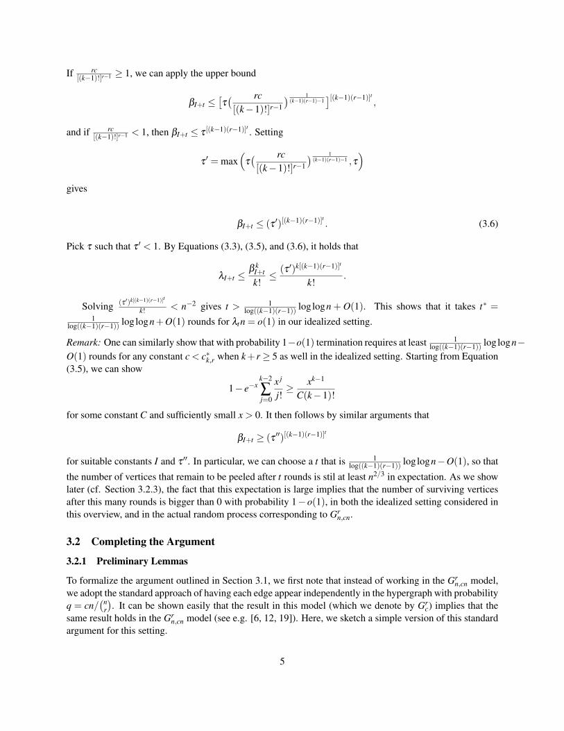
If rc[(k−1)!]r−1 ≥ 1, we can apply the upper bound

βI+t ≤[τ( rc[(k−1)!]r−1

) 1(k−1)(r−1)−1

][(k−1)(r−1)]t,

and if rc[(k−1)!]r−1 < 1, then βI+t ≤ τ [(k−1)(r−1)]t . Setting

τ′ = max

(τ( rc[(k−1)!]r−1

) 1(k−1)(r−1)−1 ,τ

)gives

βI+t ≤ (τ ′)[(k−1)(r−1)]t . (3.6)

Pick τ such that τ ′ < 1. By Equations (3.3), (3.5), and (3.6), it holds that

λI+t ≤β k

I+t

k!≤ (τ ′)k[(k−1)(r−1)]t

k!.

Solving (τ ′)k[(k−1)(r−1)]t

k! < n−2 gives t > 1log((k−1)(r−1)) log logn + O(1). This shows that it takes t∗ =

1log((k−1)(r−1)) log logn+O(1) rounds for λtn = o(1) in our idealized setting.

Remark: One can similarly show that with probability 1−o(1) termination requires at least 1log((k−1)(r−1)) log logn−

O(1) rounds for any constant c < c∗k,r when k+ r≥ 5 as well in the idealized setting. Starting from Equation(3.5), we can show

1− e−xk−2

∑j=0

x j

j!≥ xk−1

C(k−1)!

for some constant C and sufficiently small x > 0. It then follows by similar arguments that

βI+t ≥ (τ ′′)[(k−1)(r−1)]t

for suitable constants I and τ ′′. In particular, we can choose a t that is 1log((k−1)(r−1)) log logn−O(1), so that

the number of vertices that remain to be peeled after t rounds is stil at least n2/3 in expectation. As we showlater (cf. Section 3.2.3), the fact that this expectation is large implies that the number of surviving verticesafter this many rounds is bigger than 0 with probability 1−o(1), in both the idealized setting considered inthis overview, and in the actual random process corresponding to Gr

n,cn.

3.2 Completing the Argument

3.2.1 Preliminary Lemmas

To formalize the argument outlined in Section 3.1, we first note that instead of working in the Grn,cn model,

we adopt the standard approach of having each edge appear independently in the hypergraph with probabilityq = cn/

(nr

). It can be shown easily that the result in this model (which we denote by Gr

c) implies that thesame result holds in the Gr

n,cn model (see e.g. [6, 12, 19]). Here, we sketch a simple version of this standardargument for this setting.

5

Lemma 1. Let Grc be an r-uniform hypergraph on n vertices in which each edge appears independently with

probability q= cn/(n

r

). Suppose that for all c< c∗k,r, peeling succeeds on Gr

c in 1log((k−1)(r−1)) log logn+O(1)

rounds with probability 1−o(1). Then peeling similarly succeeds on Grn,cn in 1

log((k−1)(r−1)) log logn+O(1)rounds with probability 1−o(1) for all c < c∗k,r.

Proof. (Sketch) Let c′ be a constant value (independent of n) with c < c′ < c∗k,r. With probability 1−o(1), parallel peeling will succeed for the hypergraph Gr

c′ in the appropriate number of rounds. Moreover,by standard Chernoff bounds, Gr

c′ will have greater than cn edges with probability 1− o(1). Since theprobability that the parallel peeling algorithm succeeds after any number of rounds monotonically decreaseswith the addition of random edges, it holds that the success probability is also 1− o(1) when the graph ischosen from Gr

n,cn. (Formally, one would first condition on the number of edges chosen on the graph Grc′ ;

given the number of edges, the actual edges selected are random. Hence we can couple the choice of thefirst cn edges between the two graphs.)

We will also need the following lemma, which is essentially due to Voll [22]. We provide the proof forcompleteness. (We have not aimed to optimize the constants.)

Lemma 2. For any constants c,r,c1 > 0, there is a constant c2 > 0 such that with probability 1−1/n, forall vertices v in Gr

c, the neighborhood of distance c1 log logn around v contains at most logc2 n vertices.

Proof. We follow the approach used in the dissertation of Voll [22, Lemma 3.3.1]. Denote by Nd the numberof vertices at distance d in the neighborhood of a root vertex u. We prove inductively on d that

Pr(Nd > (6cr2)d log(1/ε))≤ dε

for d up to c1 log logn and ε = 1/n2. The claim then follows by a union bound over all n vertices u.For convenience we assume 6cr ≥ 1; the argument is easily modified if this is not the case, instead

proving Pr(Nd > rd log(1/ε))≤ dε . Recall that the number of edges adjacent to u is dominated by a binomialrandom variable B

((n−1r−1

),q)

, which has mean cr. The number of vertices adjacent to u via these edges isdominated by r−1 times the number of edges. When d = 1, we find that the number of neighboring edgesof the root, which we denote by N′0, is at most 6cr log(1/ε) with probability bounded above by( (n−1

r−1

)6cr log(1/ε)

)q6cr log1/ε ≤

(ecr

6cr log(1/ε)

)6cr log(1/ε)

≤ ε.

This gives an upper bound of 6cr2 log(1/ε) on N1.For the induction, we use Chernoff bounds, noting that Nd+1 can be bounded as follows. Conditioned on

the event that Nd ≤ log(1/ε)(6cr2)d , we note the number of edges adjacent to nodes of distance d is boundedabove by the sum of Nd independent binomial random variables as above, and each such edge generates atmost r−1 nodes for Nd+1. Let N′d be the number of such edges. Then we have

Pr(

Nd+1 > (6cr2)d+1 log(1/ε))≤

Pr(

Nd+1 > (6cr2)d+1 log(1/ε) | Nd > (6cr2)d log(1/ε))+

Pr(

Nd+1 > (6cr2)d+1 log(1/ε) | Nd ≤ (6cr2)d log(1/ε))≤

dε +Pr(

N′d >((6cr2)d · (6cr)

)log(1/ε) | Nd ≤ log(1/ε)(6cr2)d

).

6

We bound the last term via a Chernoff bound, noting that the sum of the Nd independent binomial randomvariables B(

(n−1r−1

),q) has the same distribution as the sum of Nd

(n−1r−1

)independent Bernoulli random vari-

ables that take value 1 with probability q. We use the Chernoff bound from [16, Theorem 4.4, part 3], whichsays that if X is the sum of independent 0-1 trials and E[X ] = µ , then for R≥ 6µ ,

Pr(X ≥ R)≤ 2−R.

Hence,

Pr(

N′d > log(1/ε)(6cr2)d · (6cr) | Nd ≤ log(1/ε)

(6cr2)d

)≤ 2− log(1/ε)(6cr2)

d ·(6cr) ≤ ε,

completing the induction and giving the lemma.

Let E be the event that the parallel peeling process on Grc terminates after 1

log((k−1)(r−1)) log logn+O(1)rounds. Our goal is to show that Pr[E] = 1−o(1). Let c1 any c2 be the constants appearing in Lemma 2. LetE1 denote the event that, for all vertices v in Gr

c, the neighborhood of distance c1 log logn around v containsat most logc2 n vertices, and let E1 denote the event that E1 does not occur.

Lemma 3. It holds that Pr[E]≥ Pr[E|E1]−1/n.

Proof. Note thatPr[E] = Pr[E|E1]Pr[E1]+Pr[E|E1]Pr[E1]. (3.7)

By Lemma 2, Pr[E]≥ 1−1/n. Hence, by Equation (3.7), Pr[E]≥ Pr[E|E1](1−1/n)≥ Pr[E|E1]−1/n.

Lemma 3 implies that, if we show that Pr[E|E1] = 1− o(1), then Pr[E] = 1− o(1) as well. This is thetask to which we now turn.

3.2.2 Completing the Proof of Theorem 1

It will help us to introduce some terminology. We will recursively refer to a vertex other than the rootas peeled in round i if it has fewer than k− 1 unpeeled children edges (that is, edges to children) at thebeginning of the round; similarly, we say that an edge e is peeled at round i if some vertex incident to e ispeeled. We refer to an edge or vertex that is not peeled as unpeeled. At round 0, all edges and vertices beginas unpeeled. For the root, we require there to be fewer than k unpeeled children edges before it is peeled.

Proof of Theorem 1. We analyze how the actual branching process deviates from the idealized branchingprocess analyzed in Section 3.1, showing the deviation leads to only lower order effects. We view thebranching process as generating a breadth first search (BFS) tree of depth at most O(log logn) rooted at theinitial vertex v. To clarify, breadth first search trees are defined such that once a vertex u is expanded in thebreadth first search, u cannot be the child of any vertex u′ in the tree that is expanded after u.

Lemma 4. When expanding a node u in the BFS tree rooted at vertex v in Grc, let Zu denote the number of

already expanded vertices in the BFS tree, and let N(u) denote the number of child edges of u in the BFStree. If Zu = polylog(n), then N(u) is a random variable with total variation distance at most polylog(n)/nfrom Poisson(rc).

7

Proof. The number of children edges incident to u in Grc is a binomial random variable B(M/q,q), where

the mean M equals(n−Zu−1

r−1

)q. Since Zu is polylogarithmic in n,

M =

(n−Zu−1

r−1

)q =

(n−1r−1

)q(1−polylog(n)/n)

= rc(1−polylog(n)/n).

We invoke Le Cam’s Theorem [13] (see Appendix A for the statement), which bounds the total variationdistance between binomial and Poisson distributions, to conclude that the total variation distance betweenB(M/q,q) and Poisson(M) is at most Mq≤ rc(cn/

(nr

))=O(1/nr−1). Meanwhile, the total variation distance

between Poisson(M) and Poisson(rc) is polylog(n)/n, and so by the triangle inequality, the total variationdistance between Poission(rc) and B(M/q,q) is also polylog(n)/n.

Lemma 5. Let X1(v) denote the random variable describing the tree of depth i = O(log logn) rooted at v inthe idealized branching process. Let X2(v) denote the random variable describing the BFS tree of depth irooted at v in Gr

c, conditioned on event E1 occurring. The total variation distance between X1(v) and X2(v)is at most polylog(n)/n.

Proof. We describe a standard coupling of the actual branching process and the idealized branching pro-cess. That is, we imagine running two different experiments (Y1(v),Y2(v)), with Y1(v) corresponding to theidealized branching process, and Y2(v) corresponding to the actual branching process conditioned on eventE1 occurring. The two branching processes will not be independent, yet Y1(v) and Y2(v) will have the samedistribution as the idealized and actual branching processes X1(v) and X2(v) respectively. We will show thatfor any i = O(log logn), with probability at least 1−polylog(n)/n the two experiments never deviate fromeach other. It follows that any event that occurs in X1(v) with probability p occurs in X2(v) with probabilityp± polylog(n)/n, and hence the total variation distance between X1(v) and X2(v) is at most polylog(n)/nas desired.

The experiments Y1(v) and Y2(v) proceed as follows. Both Y1(v) and Y2(v) begin by expanding a node v.Recall that the number of child edges of v in the idealized branching process has distribution µideal, whereµideal denotes a discrete Poisson random variable with mean rc. Let µv denote the distribution of N(v) in thereal branching process conditioned on event E1 occurring. Define αv(x) = minµideal(x),µv(x).

Let γv denote the total variation distance between µideal and µv; by Lemma 4, γv ≤ polylog(n)/n. Notethat ∑x αv(x) = 1− γv, and hence α ′v = αv/(1− γv) is a probability distribution.

At the start of experiments X1(v) and X2(v), we toss a coin with a probability of heads equal to 1− γv.If it comes up heads, we choose N from the probability distribution α ′v, and set the number of child edgesof v in both Y1(v) and Y2(v) to be N, and choose identical identifiers for their children uniformly at randomfrom [n]\v without replacement. If it comes up tails, we choose the number of child edges of v in Y1(v)according to the probability distribution σideal,v(x) defined via:

µideal(x)−µv(x)γv

if µideal(x)> µv(x)

0 otherwise,

choose the number of child edges of v in Y2(v) according to the distribution σreal,v(x) defined via:µv(x)−µideal(x)

γvif µv(x)> µideal(x)

0 otherwise,

8

and independently choose identifiers for their children at random from [n]\v, without replacement.Under these definitions, the number of child edges of v in Y1(v) is distributed according to µideal, while

the number of child edges of v in Y2(v) is distributed according to µv. That is, these quantities have thecorrect marginals, even though Y1(v) and Y2(v) are not independent.

If the coin came up tails, we then run Y1(v) and Y2(v) independently of each other for the remainder ofthe experiment. If the coin came up heads, we repeatedly expand nodes in both X1(v) and X2(v) as follows.When expanding a node u, we let µu denote the distribution of N(u) in the real branching process, and wedefine αu, γu, α ′u, σideal,u, and σreal,u analogously. We toss a new coin with a probability of heads equalto 1− γu. If the new coin comes up heads, we choose N from the probability distribution α ′u and set thenumber of child edges of u in both Y1(v) and Y2(v) to be N, and choose identical identifiers for their childrenuniformly at random from [n] \T , where T is the set of nodes already appearing in the (identical) trees. Ifthe new coin comes up tails, we choose the number of child edges of u in Y1(v) according to σideal,u, choosethe number of child edges of u in Y2(v) according to σreal,u, and independently choose the identifiers of thechildren at random from the set of nodes not already appearing in the respective tree, without replacement.

It is straightforward to check that the marginal distributions of Y1(v) and Y2(v) are the same as X1(v)and X2(v). Moreover, each time a node u is expanded in Y2(v), the processes deviate from each otherwith probability at most γu. Since X2(v) describes the actual branching process conditioned on event E1occurring, Lemma 4 guarantees that γu ≤ polylog(n)/n for all nodes u that are ever expanded. Moreover, atmost polylog(n) nodes u are ever expanded in Y2(v). By the union bound over all polylog(n) nodes u everexpanded in Y2(v), it holds that Y1(v) and Y2(v) never deviate with probability at least 1−polylog(n)/n.

Recall that λi is the probability that the root node v survives after i rounds of the idealized branchingprocess. Let λ

(a)i denote the corresponding value in the actual branching process conditioned on event E1

occurring. That is,λ(a)i = Pr[v survives i rounds of peeling in Gr

c|E1]. (3.8)

By symmetry, the probability on the right hand side of Equation (3.8) is independent of the node v.Lemma 5 implies that λi and λ

(a)i differ by at most polylog(n)/n for all i = O(log logn), and thus

λ(a)t∗ ≤ λt∗+polylog(n)/n≤ polylog(n)/n.

It remains to improve the upper bound on λ(a)i to o(1/n), as this will allow us to apply a union bound over

all the vertices v to conclude that with probability 1−o(1), no vertex survives after i rounds of peeling. Forexpository purposes, we first show how to do this assuming the neighborhood is a tree. We then show howto handle the general case, in which vertices may be duplicated as we expand the neighborhood of the rootnode v. When duplicates appear, parts of our neighborhood tree expansion are no longer independent, as inour idealized analysis, but we are able to modify the analysis to cope with these dependencies.

Bounding λi for Trees: Assume for now that the neighborhood of the root node v is a tree. Note that for theroot to be unpeeled after i rounds, there must be at least k ≥ 2 adjacent unpeeled edges, corresponding to atleast 2 (distinct, from our tree assumption) unpeeled children vertices after i−1 rounds. We have shown that,conditioned on event E1 occurring, each vertex remains unpeeled for at most t∗ = 1

log((k−1)(r−1)) log logn+O(1) rounds with probability O(polylog(n)/n). The 2 unpeeled children vertices can be chosen from theat most polylogarithmic number of children of v (the polylogarithmic bound follows from the occurrenceof event E1). This gives only

(polylog(n)2

)= polylog(n) possible sets of choices. Hence, via a union bound,

the probability that v survives at least t∗+ 1 rounds is bounded above by polylog(n) · (polylog(n)/n)2 =O(polylog(n)/n2) = o(1/n). We can take a union bound over all vertices for our final 1−o(1) bound.

9

Dealing with duplicate vertices: Finally, we now explain that, with probability 1−o(1), we need to worryonly about a single duplicate vertex in the neighborhood for all vertices, and further that this only addsan additive constant to the number of rounds required. Conditioned on event E1 occurring, for any fixednode v it holds that as we expand the neighborhood of v of distance O(log logn) using breadth first search,the probability of a duplicate vertex occurring during any expansion step is only polylog(n)/n. As theneighborhood contains only a polylogarithmic number of vertices, the probability of having at least twoduplicate vertices within the neighborhood of v is o(1/n). By a union bound over all n nodes v, withprobability 1− o(1), no node v in the graph will have two duplicated vertices in the BFS tree rooted at v.We refer to this event as E2, and we condition on this event occurring for the remainder of the proof. Thisconditioning does not affect our estimate of Pr[E|E1] by more than an additive o(1) factor, for the samereason conditioning on E1 did not affect our estimate of Pr[E] by more than an additive o(1) factor (cf.Lemma 3). Indeed,

Pr[E|E1] = Pr[E|E1∩E2]Pr[E2]+Pr[E|E1∩ E2]Pr[E2]

≥ Pr[E|E1∩E2](1−o(1)).

It is therefore sufficient to show that, conditioned on event E1 occurring, having one duplicate vertex inthe neighborhood only adds a constant number of rounds to the parallel peeling process.

We first consider the case when r ≥ 3, so that if the root remains unpeeled it has at least four (notnecessarily distinct) unpeeled vertices at distance 1 from it, corresponding to the at least two edges (eachwith at least two other vertices, as r≥ 3) that prevent the root from being peeled. If we encounter a duplicatevertex, we pessimistically assume that it prevents two vertices adjacent to the root – namely, its ancestors –from being peeled. Even with this pessimistic assumption, simply adding one additional layer of expansionin the neighborhood allows the root to be peeled by round t∗+ 2 with probability 1− o(1/n), as we nowshow.

Consider what happens in t∗+ 2 rounds when there is 1 duplicate vertex. As stated in the previousparagraph, for the root to remain unpeeled, it must have at least four neighbors, and at most two of thesefour vertices is a duplicate or has a descendant that is a duplicate. Thus, in order for the root to remainunpeeled after t∗+2 rounds, at least two neighbors, u1 and u2, of the root must remain unpeeled after t∗+1rounds, when the neighborhoods of u1 and u2 for t∗+1 rounds are trees. By our previous calculations, theprobability that u1 and u2 both remain unpeeled after t∗+ 1 rounds when their neighborhoods are trees isO(polylog(n)/n2). Thus, we take a union bound over the at most polylog(n) pairs of descendants of the root,and conclude that the probability that the root survives t∗+2 rounds of the peeling process is 1−o(1/n).

Finally, union bounding over all nodes v in Grc, we conclude that all nodes in Gr

c are peeled after t∗+2rounds with probability 1−o(1). That is, we have shown that Pr[E|E1] = 1−o(1).

The case where r = 2 and k ≥ 3 requires a bit more care. Let us consider what happens after t∗+ 3rounds in this case. For the root note v to remain unpeeled, v must have at least k ≥ 3 incident edges thatremain unpeeled after t∗+ 2 rounds of peeling. This corresponds to at least 3 (not necessarily distinct)unpeeled children of v. Thus, even if there is one duplicate vertex in the neighborhood of v, v must have atleast one unpeeled child u whose neighborhood of distance t∗+ 2 is a tree. This vertex must have at leasttwo children (grandchildren of the root) that must remain unpeeled for t∗+1 rounds. Thus, by our previouscalculations, the probability that u remains unpeeled after t∗+2 rounds is at most polylog(n)/n2. Again wecan union bound over the at most polylog(n) children u of the root node v to obtain a 1−o(1/n) probabilitythat v remains unpeeled after t∗+3 rounds in this case.

10

We have shown that Pr[E|E1] = 1−o(1), and by Equation (3.7), it follows that Pr[E] = 1−o(1) as well.

Remark: One can obtain better than 1−o(1) bounds on the probability of terminating after 1log((k−1)(r−1)) log logn+

O(1) rounds when c < c∗k,r. For example, 1−o(1/n) bounds are possible when r > 3; the argument requiresconsidering cases for the possibility that 2 vertices are duplicated in the neighborhood around a vertex.However, one cannot hope for probability bounds of 1−o(1/na) for an arbitrary constant a when duplicateedges may appear, as is typical for hashing applications. The probability the k-core is not empty because kedges share the same r vertices is Ω(n−kr+k+r) for constant k, r, and graphs with a linear number of edges,which is already Ω(1/n) for k = 2 and r = 3 or for k = 3 and r = 2.

3.2.3 Completing the Proof of Theorem 2

Recall that Theorem 2 claims that with probability 1− o(1), at least 1log((k−1)(r−1)) log logn−O(1) rounds

of peeling are required before arriving at an empty k-core. The analysis of Section 3.1 established that,in the idealized setting, each node v remains unpeeled after t = 1

log((k−1)(r−1)) log logn−C1 rounds with

probability at least n−1/3, where where C1 is an appropriately large constant that depends on k and r. Hence,in the idealized setting, the expected number of nodes that remain unpeeled after t rounds is greater than orequal to n2/3. We use this fact to establish that the claimed round lower bound holds in Gr

c with probability1−o(1).

The argument to bound the effects of deviations from the idealized process is substantially simpler inthe context of Theorem 2 than in the analogous argument from Section 3.2.2. Indeed, to prove Theorem 1,we needed to establish that with probability 1−o(1), all nodes in Gr

c are peeled after a suitable number ofrounds. The argument of Section 3.2.2 accomplished this by establishing that, for any node v, v is peeledafter t rounds with probability 1− o(1/n), for an appropriate choice of t = 1

log((k−1)(r−1)) log logn+O(1).We then applied a union bound to conclude that this holds for all nodes with probability 1− o(1). It wasrelatively easy to establish that v is peeled after t rounds with probability 1−polylog(n)/n, and most of theeffort in the proof was devoted to increasing this probability to 1−o(1/n), large enough to perform a unionbound over all n nodes.

In contrast, to establish a lower bound on the number of rounds required, one merely needs to show theexistence of a single node that remains unpeeled after t = 1

log((k−1)(r−1)) log logn−C1 rounds. Let Lt,ideal bea random variable denoting the number of nodes that remain unpeeled after t rounds in the idealized settingof Section 3.1, and let Lt be a random variable denoting the analogous number of nodes in Gr

c. As previouslymentioned, our analysis in the idealized framework (Section 3.1) shows that the expected value of Lt,idealis at least n2/3 for a suitably chosen constant C1 in the expression for t. Lemma 5 then implies that theexpected value of Lt is at least n2/3/polylog(n). We now sketch an argument that Lt is concentrated aroundits expectation, i.e., that with probability 1−o(1), Lt = E[Lt ]±n1/2polylog(n)≥ n2/3/polylog(n). We notethat an entirely analogous argument is used later to prove Theorem 3 in Section 4, where the argument isgiven in full detail.

Let E1 denote the event that there are m = cn±O(√

n logn) edges in Grc. Let E2 denote the event that

all nodes in Grc have neighbors of size at most logc2(n) for an appropriate constant c2. By Lemma 2, events

E1 and E2 both occur with probability 1−2/n. We will condition on both events occurring for the durationof the argument, absorbing an additive 2/n into the o(1) failure probability in the statement of Theorem 2(note that the conditioning causes at most an O(1) change in E[Lt ]).

We consider the process of exposing the m edges of Grc one at a time; denote the random edges by

A1,A2, . . . ,Am. For our martingale, we consider random variables Lit = E[Lt | A1, . . . ,Ai], so L0

t = E[Lt ] and

11

Lmt = Lt . Conditioned on events E1 and E2 occurring, each exposed edge changes the conditional expectation

of Lt by only logc2(n), so Azuma’s martingale inequality2 [16, Theorem 12.4] yields for sufficiently large n:

Pr(|Lt −E[Lt ]| ≥ n1/2 logc2+1(n)) ≤ 2e−n log2c2+2(n)/(2m log2c2 (n))

≤ e− log3/2(n) ≤ 1/n.

In particular, this means that with probability 1−o(1) there remain unpeeled vertices in Grc after t rounds of

peeling.

4 Above the Threshold

We now consider the case when c > c∗k,r. We show that parallel peeling requires Ω(logn) rounds in this case.Molloy [19] showed that in this case there exists a ρ > 0 such that limt→∞ ρt = ρ . Similarly, limt→∞ βt =

β > 0 and limt→∞ λt = λ > 0. It follows that the core will have size λn+o(n). We examine how βt and λt

approach their limiting values to show that the parallel peeling algorithm takes Ω(logn) rounds.

Theorem 3. Let r ≥ 3 and k ≥ 2. With probability 1− o(1), the peeling process for the k-core in Grn,cn

terminates after Ω(logn) rounds when c > c∗k,r,

Proof. First, note that β corresponds to the fixed point

β =

[1− e−β

k−2

∑j=0

β j

j!

]r−1

rc. (4.1)

Let βi = β + δi, where δi > 0. We begin by working in the idealized branching process model given inSection 3.1 to determine the behavior of βi. Starting with Equation (3.4) and considering βi+1 as a functionof δi, we obtain:

βi+1 =

[1− e−β−δi

k−2

∑j=0

(β +δi)j

j!

]r−1

rc. (4.2)

We now view the right hand side of Equation (4.2) as a function of δi. Denoting this function as f (δi),we take a Taylor series expansion around 0 and conclude that:

f (δi) = f (0)+ f ′(0)δi +Θ( f ′′(0)δ 2i ).

Equation (4.1) immediately implies that f (0) = β . Moreover, it can be calculated that

f ′(0) =(r−1)βe−β

1− e−β ∑k−2j=0

β j

j!

β k−2

(k−2)!(4.3)

In particular, it holds that0 < f ′(0)< 1. (4.4)

Note that while f ′(0) < 1 can be checked explicitly, this condition also follows immediately from theconvergence of the βi values to β .

2Formally, to cope with conditioning on events E1 and E2 in the application of Azuma’s inequality, we must actually consider aslightly modified martingale. This technique is standard, and the details can be found in Section 4.

12

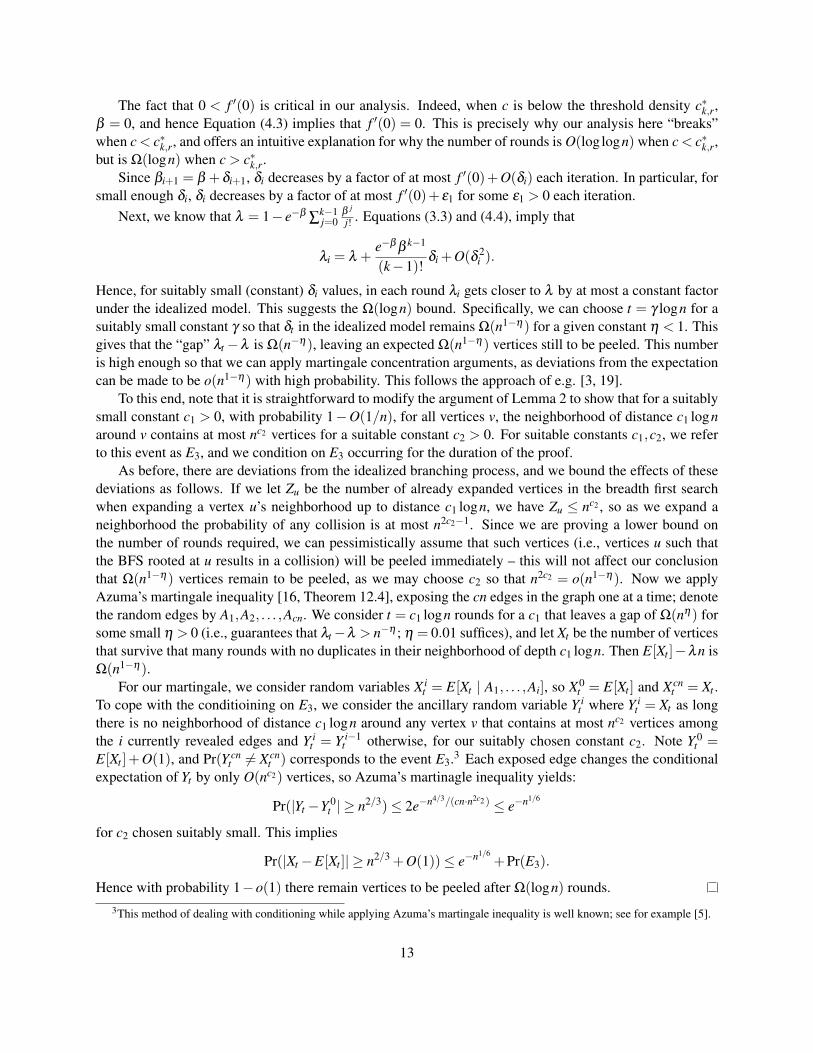
The fact that 0 < f ′(0) is critical in our analysis. Indeed, when c is below the threshold density c∗k,r,β = 0, and hence Equation (4.3) implies that f ′(0) = 0. This is precisely why our analysis here “breaks”when c < c∗k,r, and offers an intuitive explanation for why the number of rounds is O(log logn) when c < c∗k,r,but is Ω(logn) when c > c∗k,r.

Since βi+1 = β +δi+1, δi decreases by a factor of at most f ′(0)+O(δi) each iteration. In particular, forsmall enough δi, δi decreases by a factor of at most f ′(0)+ ε1 for some ε1 > 0 each iteration.

Next, we know that λ = 1− e−β∑

k−1j=0

β j

j! . Equations (3.3) and (4.4), imply that

λi = λ +e−β β k−1

(k−1)!δi +O(δ 2

i ).

Hence, for suitably small (constant) δi values, in each round λi gets closer to λ by at most a constant factorunder the idealized model. This suggests the Ω(logn) bound. Specifically, we can choose t = γ logn for asuitably small constant γ so that δt in the idealized model remains Ω(n1−η) for a given constant η < 1. Thisgives that the “gap” λt−λ is Ω(n−η), leaving an expected Ω(n1−η) vertices still to be peeled. This numberis high enough so that we can apply martingale concentration arguments, as deviations from the expectationcan be made to be o(n1−η) with high probability. This follows the approach of e.g. [3, 19].

To this end, note that it is straightforward to modify the argument of Lemma 2 to show that for a suitablysmall constant c1 > 0, with probability 1−O(1/n), for all vertices v, the neighborhood of distance c1 lognaround v contains at most nc2 vertices for a suitable constant c2 > 0. For suitable constants c1,c2, we referto this event as E3, and we condition on E3 occurring for the duration of the proof.

As before, there are deviations from the idealized branching process, and we bound the effects of thesedeviations as follows. If we let Zu be the number of already expanded vertices in the breadth first searchwhen expanding a vertex u’s neighborhood up to distance c1 logn, we have Zu ≤ nc2 , so as we expand aneighborhood the probability of any collision is at most n2c2−1. Since we are proving a lower bound onthe number of rounds required, we can pessimistically assume that such vertices (i.e., vertices u such thatthe BFS rooted at u results in a collision) will be peeled immediately – this will not affect our conclusionthat Ω(n1−η) vertices remain to be peeled, as we may choose c2 so that n2c2 = o(n1−η). Now we applyAzuma’s martingale inequality [16, Theorem 12.4], exposing the cn edges in the graph one at a time; denotethe random edges by A1,A2, . . . ,Acn. We consider t = c1 logn rounds for a c1 that leaves a gap of Ω(nη) forsome small η > 0 (i.e., guarantees that λt−λ > n−η ; η = 0.01 suffices), and let Xt be the number of verticesthat survive that many rounds with no duplicates in their neighborhood of depth c1 logn. Then E[Xt ]−λn isΩ(n1−η).

For our martingale, we consider random variables X it = E[Xt | A1, . . . ,Ai], so X0

t = E[Xt ] and Xcnt = Xt .

To cope with the conditioining on E3, we consider the ancillary random variable Y it where Y i

t = Xt as longthere is no neighborhood of distance c1 logn around any vertex v that contains at most nc2 vertices amongthe i currently revealed edges and Y i

t = Y i−1t otherwise, for our suitably chosen constant c2. Note Y 0

t =E[Xt ]+O(1), and Pr(Y cn

t 6= Xcnt ) corresponds to the event E3.3 Each exposed edge changes the conditional

expectation of Yt by only O(nc2) vertices, so Azuma’s martinagle inequality yields:

Pr(|Yt −Y 0t | ≥ n2/3)≤ 2e−n4/3/(cn·n2c2 ) ≤ e−n1/6

for c2 chosen suitably small. This implies

Pr(|Xt −E[Xt ]| ≥ n2/3 +O(1))≤ e−n1/6+Pr(E3).

Hence with probability 1−o(1) there remain vertices to be peeled after Ω(logn) rounds.3This method of dealing with conditioning while applying Azuma’s martingale inequality is well known; see for example [5].

13

c = 0.7 c = 0.75 c = 0.8 c = 0.85n Failed Rounds Failed Rounds Failed Rounds Failed Rounds10000 0 12.504 0 23.352 1000 17.037 1000 10.77320000 0 12.594 0 23.433 1000 19.028 1000 11.92840000 0 12.791 0 23.343 1000 20.961 1000 12.99280000 0 12.939 0 23.372 1000 22.959 1000 14.104160000 0 12.983 0 23.421 1000 25.066 1000 15.005320000 0 13.000 0 23.491 1000 27.089 1000 16.305640000 0 13.000 0 23.564 1000 29.281 1000 17.3341280000 0 13.000 0 23.716 1000 31.037 1000 18.4992560000 0 13.000 0 23.840 1000 33.172 1000 19.570

Table 1: Results from simulations of the parallel peeling process using r = 4 and k = 2, averaged over 1000trials.

Remark: As discussed in the introduction, the lower bound of Theorem 3 matches an O(logn) upper boundof Achiloptas and Molloy [1].

5 Simulation Results

We implemented a simulation of the parallel peeling algorithm using the Grn,cn model, in order to deter-

mine how well our theoretical analysis matches the empirical evolution of the peeling process. Our resultsdemonstrate that the theoretical analysis matches the empirical evolution remarkably well.

To check the growth of the number of rounds as a function of n, we ran the program 1000 times forr = 4,k = 2 and various values of n and c, and computed the average number of rounds for the peelingprocess to complete. For reference, c∗2,4 ≈ 0.772. Table 1 shows the results.

For all the experiments, when c < c∗2,4, all 1000 trials succeeded (empty k-core) and when c > c∗2,4, all1000 trials failed (non-empty k-core). For c < c∗2,4, the average number of rounds increases very slowlywith n, while for c > c∗2,4, the average increases approximately linearly in logn. This is in accord with ourO(log logn) result below the threshold and Ω(logn) result above the threshold. The results for other valuesof r and k were similar.

We also tested how well the idealized values from the recurrence for λt (Equation (3.1)) approximatethe fraction of vertices left after t rounds. Table 2 shows that the recurrence indeed describes the behaviorof the peeling process remarkably well, both below and above the threshold. In these simulations, we usedr = 4,k = 2 and n = 1 million. For each value of c, we averaged over 1000 trials.

6 GPU Implementation

Motivation. Using a graphics processing unit (GPU), we developed a parallel implementation for InvertibleBloom Lookup Tables (IBLTs), a data structure recently proposed by Goodrich and Mitzenmacher [9]. Twomotivating applications are sparse recovery [9] and efficiently encodable and decodable error correctingcodes [17]. For brevity we describe here only the sparse recovery application.

In the sparse recovery problem, N items are inserted into a set S, and subsequently all but n of the itemsare deleted. The goal is to recover the exact set S, using space proportional to the final number of items n,which can be much smaller than the total number of items N that were ever inserted. IBLTs achieve thisroughly as follows. The IBLT maintains O(n) cells, where each cell contains a key field and a checksum

14

c = 0.7t Prediction Experiment1 768922 7689252 673647 6736643 608076 6080974 553064 5530915 500466 5005036 444828 4448727 380873 3809308 302531 3026079 204442 20455010 93245 9339811 14159 1426912 74 7813 0.00001 014 0 015 0 016 0 017 0 018 0 019 0 020 0 0

c = 0.85t Prediction Experiment1 853158 8531722 811184 8112003 793026 7930424 784269 7842815 779841 7798516 777550 7775597 776350 7763598 775719 7757289 775385 77539410 775209 77521811 775115 77512412 775066 77507413 775039 77504814 775025 77503415 775018 77502616 775014 77502217 775012 77502018 775011 77501919 775010 77501820 775010 775018

Table 2: Simulation results evaluating how well Equation (3.1) approximates the number of vertices leftafter t rounds. The experiments are run using r = 4,k = 2,n = 1 million, averaged over 1000 trials.

field. We use r hash functions h1, . . . ,hr. When an item x is inserted or deleted from S, we consider the rcells h1(x) . . .hr(x), and we XOR the key field of each of these cells with x, and we XOR the checksum fieldof each of these cells with checkSum(x), where checkSum is some simple pseudorandom function. Noticethat the insertion and deletion procedures are identical.

In order to recover the set S, we iteratively look for “pure” cells – these are cells that only contain oneitem x in the final set S. Every time we find a pure cell whose key field is x, we recover x and delete x fromS, which hopefully creates new pure cells. We continue until there are no more pure cells, or we have fullyrecovered the set S.

The IBLT defines a random r-uniform hypergraph G, in which vertices correspond to cells in the IBLT,and edges correspond to items in the set S. Pure cells in the IBLT correspond to vertices of degree lessthan k = 2. The IBLT recovery procedure precisely corresponds to a peeling process on G, and the recoveryprocedure is successful if and only if the 2-core of G is empty.

We note that this example application is similar to other applications of peeling algorithms. For ex-ample, in the setting of erasure-correcting codes [14], encoded symbols correspond to an XOR of somenumber of original message symbols. This naturally defines a hypergraph in which vertices correspond toencoded symbols, edges correspond to unrecovered original message symbols, and a vertex can recover amessage symbol when its degree is 1. Decoding of this erasure-correcting code corresponds to peeling onthe associated hypergraph (after deleting all vertices corresponding to erased codeword symbols), and fullrecovery of the message occurs when the 2-core is empty. Our analysis directly applies to the setting whereeach message symbol randomly chooses to contribute to a fixed number r of encoded symbols.

Implementation Details. Our parallel IBLT implementation consists of two stages: the insertion/deletion

15

stage, during which items are inserted and deleted from the IBLT, and the recovery phase. Both phases canbe parallelized.

One method of parallelizing the insertion/deletion phase is as follows: we devote a separate thread toeach item to be inserted or deleted. A caveat is that multiple threads may try to modify a single cell at anypoint in time, and so we have to use atomic XOR operations, to ensure that threads trying to write to thesame cell do not interfere with each other. In general, atomic operations can be a bottleneck in any parallelimplementation; if t threads try to write to the same memory location, the algorithm will take at least t(serial) time steps. Nonetheless, our experiments showed this parallelization technique to be effective.

We parallelize the recovery phase as follows. We proceed in rounds, and in each round we devote a singlethread to each cell in the IBLT. Each thread checks if its cell is pure, and if so it identifies the item containedin the cell, removes all r occurrences of the item from the IBLT, and marks the cell as recovered. Theimplementation proceeds until it reaches an iteration where no items are recovered – this can be checkedby summing up (in parallel) the number of cells marked recovered after each round, and stopping whenthis number does not change. This procedure also requires atomic XOR operations, as two threads maysimultaneously try to write to the same cell if there are two or more items x 6= y recovered in the same roundsuch that hi(x) = hi(y) for some 1≤ i≤ r.

In addition, we must take care to avoid deleting an item multiple times from the IBLT. Indeed, sinceany item x inserted into the IBLT is placed into r cells, x might be contained in multiple pure cells at anyinstant, and the thread devoted to each such pure cell may try to delete x. This issue is not specific to theIBLT application: any implementation of the parallel peeling algorithm on a hypergraph, regardless of theapplication domain, must avoid peeling the same edge from the hypergraph multiple times.

To prevent this, we split the IBLT up into r subtables, and hash each item into one cell in each subtableupon insertion and deletion. When we execute the recovery algorithm, we iterate through the subtablesserially (which requires r serial steps per round), processing each subtable in parallel. This ensures that anitem x only gets removed from the table once, since the first time a pure cell is found containing x, x getsremoved from all the other subtables.

This recovery procedure corresponds to an interesting and fundamental variant of the peeling processwe analyze formally in Appendix B. In particular, one might initially expect that the number of (parallel)time steps required by our recovery procedure may be r times larger than the peeling process analyzed inSection 3, since our IBLT implementation requires r serial steps to iterate through all r subtables. However,we prove that the total number of parallel steps required by our IBLT implementation is roughly a factorof log2(r−1) larger than the 1

log((k−1)(r−1)) log logn+O(1) bound proved for the peeling process of Section3. This ensures that, in practice, the need to iterate serially through subtables does not create a significantserial bottleneck. Our analysis is connected in spirit to Vocking’s work on asymmetric load balancing [21],and we provide detailed discussion on the comparison between Theorems 1 and 4 in Appendix B.

Theorem 4. (Informal) Let r ≥, and φr−1 = limk→∞ F1/kr−1(k) be the growth rate for the Fibonacci sequence

of order r−1. For c < c∗k,r, peeling with sub-tables on Grn,cn terminates after

rr logφr−1+log(k−1) +O(1) sub-rounds.

We remark that while Theorem 1 holds for r = 2, k ≥ 3, Theorem 4 holds only for r ≥ 3.

Experimental Results. All of our serial code was written in C++ and all experiments were compiled withg++ using the -O3 compiler optimization flag and run on a workstation with a 64-bit Intel Xeon architectureand 48 GBs of RAM. We implemented all of our GPU code in CUDA with all compiler optimizations turnedon, and ran our GPU implementation on an NVIDIA Tesla C2070 GPU with 6 GBs of device memory.

16

Table No. Table % GPU Serial GPU SerialLoad Cells Recovered Recovery Time Recovery Time Insert Time Insert Time0.75 16.8 million 100% 0.33 s 6.37 s 0.31 s 3.91 s0.83 16.8 million 50.1% 0.42 s 3.64 s 0.35 s 4.34 s

Table 3: Results of our parallel and serial IBLT implementations with r = 3 hash functions. The table loadrefers to the ratio of the number of items in the IBLT to the number of cells in the IBLT.

Table No. Table % GPU Serial GPU SerialLoad Cells Recovered Recovery Time Recovery Time Insert Time Insert Time0.75 16.8 million 100% 0.47 s 8.37 s 0.42 s 4.55 s0.83 16.8 million 24.6% 0.25 s 2.28 s 0.46 s 5.0 s

Table 4: Results of our parallel and serial IBLT implementations with r = 4 hash functions. The table loadrefers to the ratio of the number of items in the IBLT to the number of cells in the IBLT.

Summary of results. Relative to our serial implementation, our GPU implementation achieves 10x-12xspeedups for theinsertion/deletion phase, and 20x speedups for the recovery stage when the edge density of the hypergraphis below the threshold for successful recovery (i.e. empty 2-core). When the edge density is slightly abovethe threshold for successful recovery, our parallel recovery implementation was only about 7x faster thanour serial implementation. The reasons for this are two-fold. Firstly, above the threshold, many more roundsof the parallel peeling process were necessary before the 2-core was found. Secondly, above the threshold,less work was required of the serial implementation because fewer items were recovered; in contrast, theparallel implementation examines every cell in every round.

Our detailed experimental results are given in Tables 3 (for the case of r = 3 hash functions) and 4(for the case of r = 4 hash functions). The timing results are averages over 10 trials each. For the GPUimplementation, the reported times do count for the time to transfer data (i.e. the items to be inserted) fromthe CPU to the GPU.

The reported results are for a fixed IBLT size, consisting of 224 cells. These results are representativefor all sufficiently large input sizes: once the number of IBLT cells is larger than about 219, the runtime ofour parallel implementation grows roughly linearly with the number of table cells (for any fixed table load).Here, table load refers to the ratio of the number of items in the IBLT to the number of cells in the IBLT. Thiscorresponds to the edge density c in the corresponding hypergraph. The linear increase in runtime above acertain input size is typical, and is due to the fact that there is a finite number of threads that the GPU canlaunch at any one time.

7 Rounds as a Function of the Distance from the Threshold

Recall that the hidden constant in the O(1) term of Theorem 1 depends on the size of the “gap” ν = c∗k,r− cbetween the edge density and the threshold density. This term can be significant in practice when ν is small,and in this section, we make the dependence on ν explicit. Specifically, we extend the analysis of Section3 to characterize how the growth of the number of rounds depends on c∗k,r− c, when c is a constant withc < c∗k,r. The proof of Theorem 5 below is in Appendix C.

Theorem 5. Let ν = |c∗k,r−c| for constant c with c< ck,r. With probability 1−o(1), peeling in Grn,cn requires

Θ(√

1/ν)+ 1log((k−1)(r−1)) log logn rounds when c is below the threshold density c∗k,r.

17

8 Conclusion

In this paper, we analyzed parallel versions of the peeling process on random hypergraphs. We showedthat when the number of edges is below the threshold edge density for the k-core to be empty, with highprobability the parallel algorithm takes O(log logn) rounds to peel the k-core to empty. In contrast, when thenumber of edges is above the threshold, with high probability it takes Ω(logn) rounds for the algorithm toterminate with a non-empty k-core. We also considered some of the details of implementation and proposeda variant of the parallel algorithm that avoids a fundamental implementation issue; specifically, by usingsubtables, we avoid peeling the same element multiple times. We show this variant converges significantlyfaster than might be expected, thereby avoiding a sequential bottleneck. Our experiments confirm our the-oretical results and show that in practice, peeling in parallel provides a considerable increase in efficiencyover the serialized version.

References

[1] D. Achlioptas and M. Molloy. The solution space geometry of random linear equations. RandomStructures and Algorithms (to appear), 2013.

[2] Y. Azar, A. Broder, A. Karlin, and E. Upfal. Balanced allocations. SIAM Journal of Computing29(1):180–200, 1999.

[3] A. Broder, A. Frieze, and E. Upfal. On the satisfiability and maximum satisfiability of random 3-CNFformulas. In Proc. of the Fourth Annual ACM-SIAM Symposium on Discrete Algorithms, pp. 322–330,1993.

[4] B. Chazelle, J. Kilian, R. Rubinfeld, and A. Tal. The Bloomier filter: an efficient data structure for staticsupport lookup tables. In Proc. of the Fifteenth Annual ACM-SIAM Symposium on Discrete Algorithms,pp. 30–39, 2004.

[5] F. Chung and L. Lu. Concentration inequalities and martingale inequalities: a survey. Internet Mathe-matics, 3(1):79-127, 2006.

[6] M. Dietzfelbinger, A. Goerdt, M. Mitzenmacher, A. Montanari, R. Pagh, and M. Rink. Tight thresholdsfor cuckoo hashing via XORSAT. In Proc. of ICALP, pp. 213–225, 2010.

[7] D. Eppstein, M. Goodrich, F Uyeda, and G. Varghese. What’s the Difference? Efficient Set Reconcili-ation without Prior Context. ACM SIGCOMM Computer Communications Review (SIGCOMM 2011),41(4):218–229, 2011.

[8] P. Gao. Analysis of the parallel peeling algorithm: a short proof. arXiv:1402.7326, 2014.

[9] M. Goodrich and M. Mitzenmacher. Invertible Bloom Lookup Tables. In Proc. of the 49th AllertonConference, pp. 792–799, 2011.

[10] J. Jiang, M. Mitzenmacher, J. Thaler. Parallel Peeling Algorithms. CoRR abs/1302.7014, 2013.

[11] R. Karp, M. Luby, and F. Meyer auf der Heide. Efficient PRAM simulation on a distributed memorymachine. Algorithmica, 16(4):517–542, 1996.

18

[12] A. Kirsch, M. Mitzenmacher, and U. Wieder. More robust hashing: Cuckoo hashing with a stash. SIAMJournal on Computing, 39(4):1543-1561, 2009.

[13] L. Le Cam. An approximation theorem for the Poisson binomial distribution. Pacific Journal of Math-ematics 10(4):1181-1197, 1960.

[14] M. Luby, M. Mitzenmacher, A. Shokrollahi, and D. Spielman. Efficient erasure correcting codes. IEEETransactions on Information Theory, 47(2):569–584, 2001.

[15] M. Mitzenmacher. The power of two choices in randomized load balancing. IEEE Transactions onParallel and Distributed Systems, 12(10):1094–1104, 2001.

[16] M. Mitzenmacher and E. Upfal. Probability and computing: Randomized algorithms and proba-bilistic analysis, 2005, Cambridge University Press.

[17] M. Mitzenmacher and G. Varghese. Biff (Bloom filter) codes: Fast error correction for large data sets.In Proc. of the IEEE International Symposium on Information Theory, pp. 483–487, 2012.

[18] M. Mitzenmacher and B. Vocking. The asymptotics of selecting the shortest of two, improved. Proc. ofthe 37th Annual Allerton Conference on Communication Control and Computing, pp. 326–327, 1999.

[19] M. Molloy. The pure literal rule threshold and cores in random hypergraphs. In Proc. of the 15th AnnualACM-SIAM Symposium on Discrete Algorithms, pp. 672–681, 2004.

[20] A. Pagh and F. Rodler. Cuckoo hashing. Journal of Algorithms, 51(2):122–144, 2004.

[21] B. Vocking. How asymmetry helps load balancing, Journal of the ACM, 50(4):568–589, 2003.

[22] U. Voll. Threshold Phenomena in Branching Trees and Sparse Random Graphs. Dissertation. Techis-chen Universitat Munchen. 2001.

A Le Cam’s Theorem

Le Cam’s Theorem can be stated as follows.

Theorem 6. Let X1,X2, . . . ,Xn be independent 0-1 random variables with Pr(Xi = 1) = pi. Let λ = ∑ni=1 pi

and S = ∑ni=1 Xi. Then

∞

∑k=0|Pr(S = k)− e−λ

λk/k!|< 2

n

∑i=1

p2i .

In particular, when pi = λ/n for all i, we obtain that the binomial distribution converges to the Poissondistribution, with total variation distance bounded by λ 2/n.

B Parallel Peeling with Subtables

The parallel peeling process used in our GPU implementation of IBLTs in Section 6 does not preciselycorrespond to the one analyzed in Sections 3.2 and 4. The differences are two-fold. First, the underlyinghypergraph G in our IBLT implementation is not chosen uniformly from all r-uniform hypergraphs; instead,vertices in G (i.e., IBLT cells) are partitioned into r equal-sized sets (or subtables) of size n/r, and edges

19

are chosen at random subject to the constraint that each edge contains exactly one vertex from each set.Second, the peeling process in our GPU implementation does not attempt to peel all vertices in each round.Instead, our GPU implementation proceeds in subrounds, where each round consists of r subrounds. In theith subround of a given round, we remove all the vertices of degree less than k in the ith subtable. Note thatrunning one round of this algorithm is not equivalent to running one round of the original parallel peelingalgorithm. This is because peeling the first subtable may free up new peelable vertices in the second subtable,and so on. Hence, running one round of the algorithm used in our GPU implementation may remove morevertices than running one round of the original algorithm.

In this section, we analyze the peeling process used in our GPU implementation. We can use a similarapproach as above to obtain the recursion for the survival probabilities for this algorithm. Let ρi, j be theprobability that a vertex in the tree survives i rounds when it’s in the jth subtable, with each ρ0, j = 1. Then,

ρi, j = Pr(

Poisson(

rc∏h< j

ρi,h ∏h> j

ρi−1,h

)≥ k−1

).

By the same reasoning,

λi, j = Pr(

Poisson(

rc∏h< j

ρi,h ∏h> j

ρi−1,h

)≥ k)

(B.1)

where λ0, j = 1 for all j. Also, we can consider

βi, j = rc(

∏h< j

ρi,h

)(∏h> j

ρi−1,h

).

These equations differ from our original equation in a way similar to how the equations for standard multiple-choice load-balancing differ from Vocking’s asymmetric variation of multiple-choice load-balancing, wherea hash table is similarly split into r subtables, each item is given one choice by hashing in each subtable,and the item is placed in the least loaded subtable, breaking ties according to some fixed ordering of thesubtables [18, 21].

Motivated by this, we can show that in this variation, below the threshold, these values eventually de-crease “Fibonacci exponentially”, that is, with the exponent falling according to a generalized Fibonaccisequence. We follow the same approach as outlined in Section 3.1. Let β ′m = βi, j where m = (i− 1)r+ j,and similarly for λ ′m and ρ ′m, so we may work in a single dimension. Let Fr−1(i) represent the ith numberin a Fibonacci sequence of order r− 1. Here, a Fibonacci sequence of order r is defined such that the firstr− 1 elements in the sequence equal one, and for i > r− 1, the ith element is defined to be the sum of thepreceding r−1 terms.

We choose a constant I so that β ′I+a ≤ φ Fr−1(a) for an appropriate constant φ < 1 and 0≤ a≤ r−1. Weinductively show that

β′I+t ≤ φ

(k−1)bt/rcFr−1(t)

when rc[(k−1)!]r−1 < 1; as in Section 3, the proof can be modified easily if rc

[(k−1)!]r−1 > 1 by simply choosing a

20

different (constant) starting point I for the induction. In this case, for t ≥ r

β′I+t ≤

[∏

I+t−r< j<I+t

(β ′j)k−1

(k−1)!

]rc

≤ rc[(k−1)!]r−1 ∏

I+t−r< j<I+t(β ′j)

k−1

≤ rc[(k−1)!]r−1 ∏

I+t−r< j<I+t

(φ

Fr−1( j)(k−1)b(t−r)/rc)(k−1)

≤ φ(k−1)bt/rcFr−1(t). (B.2)

Thus, our induction yields that the exponent of φ in the β ′m values falls according to a generalizedFibonacci sequence of order r− 1, leading to an asymptotic constant factor reduction in the number ofoverall rounds, even as we have to work over a larger number of subrounds. Inequality (B.2) applies tothe idealized branching process, but we can handle deviations between the idealized process and the actualprocess essentially as in Theorem 1. This yields the following variation of Theorem 1 for the setting ofpeeling with sub-tables.

Theorem 7. Let r≥ 3 and k≥ 2. Let φr−1 = limk→∞ F1/kr−1(k) be the asymptotic growth rate for the Fibonacci

sequence of order r− 1. Let G be a hypergraph over n nodes with cn edges generated according to thefollowing random process. The vertices of G are partitioned into r subsets of equal size, and the edges aregenerated at random subject to the constraint that each edge contains exactly one vertex from each set.

With probability 1− o(1), the peeling process for the k-core in G that uses r subrounds in each roundterminates after

1r logφr−1+log(k−1) log logn+O(1) rounds when c < c∗k,r.

It is worth performing a careful comparison of Theorems 1 and 7. For simplicity, we will restrict thediscussion to k = 2. This corresponds to the case where we are interested in the 2-core of the hyper-graph, as in our IBLT implementation. Theorem 1 guarantees that the peeling process of Section 3 requires

1log(r−1) log logn+O(1). Meanwhile, Theorem 7 guarantees that the total number of sub-rounds required by

our IBLT implementation is r · 1r logφr−1

log logn+O(1) = 1logφr−1

log logn+O(1). Thus, parallel peeling withsubtables takes a factor log(r−1)/ log(φr−1) more (sub)-rounds than parallel peeling without subtables.

For r = 3, φr−1 ≈ 1.61 is the golden ratio, and in this case log(r− 1)/ log(φr−1) ≈ 1.456. Thus, forr = 3 and k = 2, parallel peeling with sub-tables takes a factor of less than 1.5 times more (sub)-rounds thanparallel peeling. In contrast, one might a priori have expected that the number of sub-rounds for peelingwith sub-tables would be a factor r = 3 larger than in the standard peeling process, since r serial steps arerequired to iterate through all r subtables.

As r grows, φr−1 rapidly approaches 2 from below. For example, for r = 4 this quantity is approximately1.83 and for r = 5 it is approximately 1.92 [21]. It follows that for large r the ratio log(r−1)/ log(φr−1) isvery close to log2(r−1).

Simulations with Subtables

We ran simulations for the parallel peeling algorithm with subtables in a similar way as the simulations inSection 5. Table 5 shows the results for the average number of subrounds. The number of subrounds is atmost r times the number of rounds in the original parallel peeling algorithm, but our analysis of Section B

21

c = 0.7 c = 0.75n Failed Subrounds Failed Subrounds10000 0 26.018 0 47.73220000 0 26.142 0 47.65940000 0 26.273 0 47.66680000 0 26.452 0 47.783160000 0 26.585 0 47.769320000 0 26.790 0 47.925640000 0 26.957 0 48.0701280000 0 27.006 0 48.1412560000 0 27.012 0 48.175

Table 5: Results of simulations of peeling with subtables using r = 4 and k = 2, over 1000 trials.

suggests the number of subrounds should be significantly smaller. In this case, comparing Table 5 withTable 1, this factor is about 2.

We also performed simulations to determine how closely the recursion given in Equation (B.1) predictsthe number of vertices left after peeling the jth subtable in the ith round. Denote by λ ′i, j the expected fractionof vertices left in the (i, j)’th subround. Then λ ′i, j is given by the following formula:

λ′i, j =

1r

(∑h≤ j

λi,h + ∑h> j

λi−1,h

),

where the λi, j values are given by Equation (B.1). The results are presented in Table 6, where the predictioncolumn reports the values of λ ′i, jn. As can be seen, the prediction closely matches the number of verticesleft in the simulation.

C Proof of Theorem 7.1

We recall the statement of Theorem 5, before offering a proof.

Theorem 5. Let ν = |c∗k,r − c| for constant c with c < ck,r. With probability 1− o(1), peeling in Grn,cn

requires Θ(√

1/ν)+ 1log((k−1)(r−1)) log logn rounds when c is below the threshold density c∗k,r.

Since k and r are constants, for notational convenience, we use c∗ in place of c∗k,r where the meaning isclear. Recall that we are working in the setting where ν = c∗−c > 0. Recall Equation (2.1) for c∗ and let x∗

be the value of x that satisfies c∗ = xr(1−e−x ∑

k−2j=0

x jj! )

r−1. Intuitively, one may think of x∗ as the expected number

of surviving descendant edges of each node in the graph when the edge density c is precisely equal to thethreshold density c∗.

The heart of our analysis lies in proving the following lemma.

Lemma 6. Let τ < x∗ be any constant. It takes Θ(√

1/ν) rounds before βi < τ .

22

c = 0.7i j Prediction Experiment1 1 942230 9422301 2 876807 8768031 3 801855 8018551 4 714875 7148782 1 678767 6787712 2 643070 6430802 3 609686 6096972 4 581912 5819193 1 554402 5544143 2 527335 5273413 3 500469 5004763 4 472470 4724754 1 442874 4428714 2 410958 4109564 3 375770 3757644 4 336458 3364475 1 292159 2921445 2 242396 2423745 3 187891 1878665 4 131789 1317766 1 80372 803766 2 40582 406006 3 15481 155036 4 3649 36667 1 348 3547 2 6 67 3 0.003 0.0087 4 0 0

Table 6: Results of simulations of peeling with subtables showing how well the recursion for λ ′i, j approximates thenumber of vertices left after t rounds. The experiments are run using r = 4,k = 2,n = 1 million, averaged over 1000trials.

23

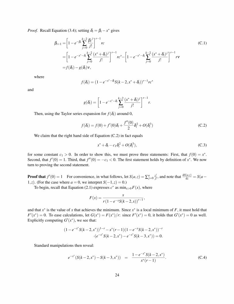
Proof. Recall Equation (3.4); setting δi = βi− x∗ gives

βi+1 =

[1− e−βi

k−2

∑j=0

βij

j!

]r−1

rc (C.1)

=

[1− e−x∗−δi

k−2

∑j=0

(x∗+δi)j

j!

]r−1

rc∗−[

1− e−x∗−δik−2

∑j=0

(x∗+δi)j

j!

]r−1

rν

= f (δi)−g(δi)ν ,

wheref (δi) = (1− e−x∗−δiS(k−2,x∗+δi))

r−1rc∗

and

g(δi) =

[1− e−x∗−δi

k−2

∑j=0

(x∗+δi)j

j!

]r−1

r.

Then, using the Taylor series expansion for f (δi) around 0,

f (δi) = f (0)+ f ′(0)δi +f ′′(0)

2δ

2i +O(δ 3

i ) (C.2)

We claim that the right hand side of Equation (C.2) in fact equals

x∗+δi− c1δ2i +O(δ 3

i ), (C.3)

for some constant c1 > 0. In order to show this, we must prove three statements: First, that f (0) = x∗.Second, that f ′(0) = 1. Third, that f ′′(0) =−c1 < 0. The first statement holds by definition of x∗. We nowturn to proving the second statement.

Proof that f ′(0) = 1 For convenience, in what follows, let S(a,z) = ∑aj=0

z j

j! , and note that dS(a,z)dz = S(a−

1,z). (For the case where a = 0, we interpret S(−1,z) = 0.)To begin, recall that Equation (2.1) expresses c∗ as minx>0 F(x), where

F(x) =x

r (1− e−xS(k−2,x))r−1 ,

and that x∗ is the value of x that achieves the minimum. Since x∗ is a local minimum of F , it must hold thatF ′(x∗) = 0. To ease calculations, let G(x∗) = F(x∗)/r: since F ′(x∗) = 0, it holds that G′(x∗) = 0 as well.Explicitly computing G′(x∗), we see that:

(1− e−x∗S(k−2,x∗))1−r− x∗(r−1)(1− e−xS(k−2,x∗))−r

·(e−x∗S(k−2,x∗)− e−x∗S(k−3,x∗)) = 0.

Standard manipulations then reveal:

e−x∗(S(k−2,x∗)−S(k−3,x∗)) =1− e−x∗S(k−2,x∗)

x∗(r−1). (C.4)

24

Now recall thatf (δi) = (1− e−x∗−δiS(k−2,x∗+δi))

r−1rc∗.

It follows that

f ′(0)

= (r−1)rc∗(1− e−x∗S(k−2,x∗))r−2e−x∗(S(k−2,x∗)−S(k−3,x∗))

=rc∗

x∗(1− e−x∗S(k−2,x∗))r−1 (C.5)

=1. (C.6)

Here Equation (C.5) follows from Equation (C.4), and Equation (C.6) follows from the definition of c∗ andx∗ according to Equation (2.1).

Proof that f ′′(0)< 0 After some tedious but straightforward calculations, we find that

f ′′(0) =r−2

(r−1)x∗−1+

k−2x∗

. (C.7)

We therefore have that f ′′(0)< 0 as long as

x∗ > k−1− 1r−1

. (C.8)

Our argument will proceed as follows. Equation (2.1) implies that x∗ is a local minimum of the functionZ(x) = x

(1−e−xS(k−2,x))r−1 . We will compute Z′(x), and show that for Z′(x) < 0 for all x ∈ (0,k− 1) for anyr ≥ 3. It will follow that x∗ ≥ k−1, and hence Inequality (C.8) holds. Details follow.

It suffices to consider the function rZ(x) = x(1− e−xS(k− 2,x))1−r, as the derivative of rZ(x) alwayshas the sign as Z(x). The derivative of rZ(x) is (

1− e−xS(k−2,x))1−r

+

x(1− r)(1− e−xS(k−2,x)

)−r · e−x (S(k−2,x)−S(k−3,x)) =(1− e−xS(k−2,x)

)−r

·[(

1− e−xS(k−2,x))+ xk−1e−x(1− r)/((k−2)!)

]. (C.9)

We will show this the above expression is negative for all x ∈ (0,k− 1). Note that 1− e−xS(k− 2,x) =e−x

∑∞j=k−1 x j/ j! > 0. Hence, multiplying Expression (C.9) through by (1− e−xS(k−2,x))rex, we find the

derivative is negative when(r−1)xk−1

(k−2)!>

∞

∑j=k−1

x j/ j!.

Notice that the left hand side is (r− 1)(k− 1) ≥ 2(k− 1) times the first term of the right hand side, andfor x < k− 1, the terms in the summation on the right hand side are decreasing. In fact, after k− 1 terms,the sum on the right hand side is dominated by a geometric series in which each term decreases by a factorof 1/2. It follows that right hand sum is less than 2(k− 1) times the first term, and hence the derivative isnegative for all x ∈ (0,k−1). This completes the proof that f ′′(0)< 0, and we conclude that Equation (C.3)holds.

25

Equation (C.3) combined with Taylor’s Theorem implies that there exists some h(δi) such that f (δi) =x∗+ δi− c1δ 2

i + h(δi)δ2i , where limδi→0 h(δi) = 0. This means there exist constants c′1,c

′′1 > 0 such that

x∗+δi− c′1δ 2i < f (δi)< x∗+δi− c′′1δ 2

i for |δi| less than a suitably chosen small constant.In the same way, we can find constants c′2,c

′′2 > 0 such that c′2 < g(δi) < c′′2 for |δi| less than a suitably

small constant. Since βi+1 = x∗+δi+1, we can examine the following recurrence for δi+1:

δi+1 = δi− c1δ2i − c2ν

δ0 = r(c∗−ν)− x∗,

where c1,c2 > 0.Again, we can upper bound δ0 by a suitably small constant by taking ν small enough. Next, we show it

takes Θ(√

1/ν) rounds for δi < τ− x∗, proving the lemma. (Note τ− x∗ < 0.) We break the problem intothree substeps: the number of rounds it takes to get from δ0 to Θ(

√ν), from Θ(

√ν) to −Θ(

√ν), and from

−Θ(√

ν) to τ− x∗.

From Θ(√

ν) to −Θ(√

ν): Since |δi| = Θ(√

ν), from the recursion, Θ(ν) is subtracted from δi in eachround. Since this interval has length Θ(

√ν), it takes Θ(

√ν)

Θ(ν) = Θ(√

1/ν) rounds for this substep.

From δ0 to Θ(√

ν): Since δi = Ω(√

ν), each round Ω(ν) is subtracted from δi. Intuitively, this means wemay ignore the −c2ν term, and the recursion becomes

δ′i+1 = δ

′i − c1(δ

′i )

2

for a suitable constant c1 > 0, with δ ′0 = δ0. More formally, since c2,ν > 0, the sequence of δ ′i values requiremore rounds to reach Θ(

√ν) than the sequence of δi values, so analyzing this recursion provides an upper

bound on the number of rounds for λi to fall from δ0 to Θ(√

ν).Let δ ′′i = c1δ ′i . Then the recursion can be rewritten as

δ′′i+1 = δ

′′i (1−δ

′′i ).

Let γi = 1/δ ′′i . Then γi+1 = γi + 1+ 1γi−1 , which implies γi > γ0 + i. For any ν ′ > 0, take N such that

1/(N− 1) < ν ′. Then since γi > i, for all i > N, γi+1 < γi + 1+ν ′ and γi < (1+ν ′)i for sufficiently largei. Therefore, γi = (1+o(1))i and δ ′′i = 1+o(1)

i . Thus, it takes i = O(√

1/ν) rounds for δ ′′i (and hence δi) toreach Θ(

√ν).

From −Θ(√

ν) to τ− x∗: By the same reasoning as the previous case, consider the recursion

δ′′i+1 = δ

′′i (1−δ

′′i ).

Consider the sequence backwards; the number of rounds from −Θ(√

ν) to τ− x∗ is equivalent to the num-ber of rounds for the “backwards” recursion, starting from τ − x∗ and going to −Θ(

√ν). The backwards

recursion can be obtained by solving the quadratic equation for δ ′′i :

δ′′i =

1−√

1−4δ ′′i+1

2.

We can reverse the negative signs and look at the following recursion

γi+1 =

√1+4γi−1

2;

γ0 = x∗− τ.

26

Figure 1: Behavior of the βi according to the idealized recurrence of Equation (C.1) at values of c close tothe threshold density c∗2,4 ≈ .77228.

The Taylor series expansion for√

1+4x−12 reveals that

√1+4x−1

2 = x− x2 +O(x3), and it can be shown that√1+4x−1

2 < x− 12 x2 for 0 < x < 2−

√2. It takes a constant number of steps to get from γ0 = x∗−τ to 2−

√2,

and then we can upper bound the number of steps needed by this recursion to reach Θ(√

ν) by the recursionγ ′i+1 = γ ′i − 1

2(γ′i )

2. As with the previous case, it takes O(√

1/ν) rounds for γi to reach Θ(√

ν).

We note that, again, the above analysis focuses on the idealized process, but we can handle deviationsbetween the idealized process and the actual process essentially as in Theorem 1.

Theorem 5 follows readily. Choose τ satisfying

τ <( rc∗

[(k−1)!]r−1

)− 1(k−1)(r−1)−1

and τ < 1. By Lemma 6, it takes Θ(√

1/ν) rounds before βi < τ . The argument in Section 3.1 shows thatin the idealized branching process, βi drops off doubly exponentially in the number of rounds after that,giving the 1

log((k−1)(r−1)) log logn additive term. Finally, the argument in the proof of Theorem 1 shows thatdeviations from the idealized process result in O(1) additional rounds with high probability.

Our three-phase analysis appears to accurately capture the empirical evolution of the idealized recursion.For example, Figure 1 shows the behavior of βi according to the idealized recurrence of Equation (C.1)for selected values of c close to the threshold when k = 2 and r = 4. In this case the threshold c∗2,4 isapproximately 0.77228, and we show the evolution of βi at c = 0.77 and c = .772. The long “stretch” in themiddle of the plots corresponds to the Θ(

√1/ν) rounds required during “middle phase” in our argument,

in which βi falls from (Θ(√

1/ν) to −Θ(√

1/ν).

27