parallel preconditioners for finite element computations
TRANSCRIPT

College of Saint Benedict and Saint John's University College of Saint Benedict and Saint John's University
DigitalCommons@CSB/SJU DigitalCommons@CSB/SJU
Honors Theses, 1963-2015 Honors Program
4-2015
Parallel Preconditioners for Finite Element Computations Parallel Preconditioners for Finite Element Computations
Emily Furst College of Saint Benedict/Saint John's University
Follow this and additional works at: https://digitalcommons.csbsju.edu/honors_theses
Part of the Computer Sciences Commons, and the Mathematics Commons
Recommended Citation Recommended Citation Furst, Emily, "Parallel Preconditioners for Finite Element Computations" (2015). Honors Theses, 1963-2015. 66. https://digitalcommons.csbsju.edu/honors_theses/66
This Thesis is brought to you for free and open access by DigitalCommons@CSB/SJU. It has been accepted for inclusion in Honors Theses, 1963-2015 by an authorized administrator of DigitalCommons@CSB/SJU. For more information, please contact [email protected].

Parallel Preconditioners for Finite
Element ComputationsAN HONORS THESIS
College of Saint Benedict/Saint John’s University
In Partial Fulfillment
of the Requirements for Distinction
In the Departments of Computer Science and Mathematics
by Emily Furst
April 2015

PROJECT TITLE: Parallel Preconditioners for Finite Element Computations
Approved by:
Michael Heroux
Scientist in Residence of Computer Science
Imad Rahal
Associate Professor of Computer Science
Robert Hesse
Associate Professor of Mathematics
Imad Rahal
Chair, Department of Computer Science
Robert Hesse
Chair, Department of Mathematics
Emily Esch
Director, Honors Thesis Program
1

Abstract
This thesis sought to explore numerical methods for solving partial differential equations
and to determine the best method of updating the deal.II software to utilize new Trilinos
software packages. The one dimensional heat equation with Dirichlet boundary conditions
and nonzero initial conditions was solved analytically, using the Forward in Time, Central
in Space scheme of the finite difference method, and the Crank-Nicolson scheme of the finite
element method. The solutions from using the finite difference method and the finite element
method were then compared to the analytic solution to determine accuracy. An example
using the same Trilinos packages that are utilized in deal.II currently was updated to use the
newer Trilinos packages to determine how to update deal.II and to analyze any performance
increases resulting from these changes to the software.
2

Contents
1 Introduction 5
1.1 Introduction to Partial Differential Equations and the One Dimensional Heat Equa-
tion . . . . . . . . . . . . . . . . . . . . . . . . . . . . . . . . . . . . . . . . . . . . 5
1.2 Introduction to Parallel and Distributed Computing . . . . . . . . . . . . . . . . . 6
2 Contributions to this Topic 7
3 Problem Statement 7
4 Background 8
4.1 Analytical Solutions and Separation of Variables . . . . . . . . . . . . . . . . . . . 8
4.2 The Finite Difference Method . . . . . . . . . . . . . . . . . . . . . . . . . . . . . . 9
4.3 The Finite Element Method . . . . . . . . . . . . . . . . . . . . . . . . . . . . . . . 10
4.4 Trilinos Software . . . . . . . . . . . . . . . . . . . . . . . . . . . . . . . . . . . . . 11
4.4.1 Epetra, Tpetra, and Xpetra . . . . . . . . . . . . . . . . . . . . . . . . . . . 11
4.4.2 ML and MueLu . . . . . . . . . . . . . . . . . . . . . . . . . . . . . . . . . . 12
4.4.3 AztecOO and Belos . . . . . . . . . . . . . . . . . . . . . . . . . . . . . . . 12
4.4.4 Summary of Trilinos Packages . . . . . . . . . . . . . . . . . . . . . . . . . . 13
4.5 deal.II Software . . . . . . . . . . . . . . . . . . . . . . . . . . . . . . . . . . . . . . 13
5 Methods 14
5.1 Source Code and Computing Architecture . . . . . . . . . . . . . . . . . . . . . . . 14
5.2 Solving the One Dimensional Heat Equation Analytically . . . . . . . . . . . . . . 14
5.3 Solving Using FTCS Finite Differences . . . . . . . . . . . . . . . . . . . . . . . . . 17
5.4 Solving Using Crank-Nicolson FEM . . . . . . . . . . . . . . . . . . . . . . . . . . 18
5.5 Developing a Method for Updating the deal.II Software . . . . . . . . . . . . . . . 19
6 Results 20
6.1 One-Dimensional Heat Equation Results . . . . . . . . . . . . . . . . . . . . . . . . 20
6.1.1 Analytical Solution . . . . . . . . . . . . . . . . . . . . . . . . . . . . . . . . 20
6.1.2 Finite Difference Results . . . . . . . . . . . . . . . . . . . . . . . . . . . . . 22
6.1.3 Finite Element Method Results . . . . . . . . . . . . . . . . . . . . . . . . . 28
6.2 Small Scale Example Results . . . . . . . . . . . . . . . . . . . . . . . . . . . . . . 30
3
7 Conclusion 37
7.1 Future Work . . . . . . . . . . . . . . . . . . . . . . . . . . . . . . . . . . . . . . . 38
8 Appendix 40
8.1 Computing Architecture . . . . . . . . . . . . . . . . . . . . . . . . . . . . . . . . . 40
8.2 MLAztecOO.cpp Source Code . . . . . . . . . . . . . . . . . . . . . . . . . . . . . . 40
8.3 MLBelos.cpp Source Code . . . . . . . . . . . . . . . . . . . . . . . . . . . . . . . . 44
8.4 MueLuBelos.cpp Source Code . . . . . . . . . . . . . . . . . . . . . . . . . . . . . . 48
8.5 Makefile for MLAztecOO.cpp . . . . . . . . . . . . . . . . . . . . . . . . . . . . . . 54
8.6 Trilinos cmake Script . . . . . . . . . . . . . . . . . . . . . . . . . . . . . . . . . . . 56
8.7 deal.II Install Notes . . . . . . . . . . . . . . . . . . . . . . . . . . . . . . . . . . . 56
4

1 Introduction
Many of the problems that are of interest to scientists regarding the physical world can best be
described by a partial differential equation. Heat dynamics, fluid dynamics, and quantum me-
chanics can all be described in terms of partial differential equations. However, partial differential
equations can be quit difficult and time-consuming to solve analytically. Here, solving analytically
refers to using algebraic or numeric methods to find a solution to a partial differential equation
where the solution is in the form of an equation. As a result, many softwares have been developed
in order to make the solving of such problems easier. However, as computers cannot process the
infinite number of points comprising a problem space, finite numerical algorithms were developed
to replace traditional analytical methods. These computational methods vary in terms of efficiency
and accuracy.
One particular application of computational methods is in the solving of very large problems.
This desire to solve exceptionally large problem sizes has led to the development of high perfor-
mance and parallel methods of solving. Many numerical methods involve quite a bit of repetition
in computation which enables the programmer to exploit quite a bit of parallelism. Well thought
out and smart storage patterns of data in memory can also be utilized to improve performance.
When parallel and high performance methods are implemented well, increased time performance
is often noted in the computation time associated with solving such large problems.
1.1 Introduction to Partial Differential Equations and the One Dimen-
sional Heat Equation
Partial differential equations (PDEs) are highly important tools for the understanding of the
physical world, and in fact were formulated by scientists in the eighteenth and nineteenth centuries
in order to describe different aspects of the physical world [11]. It is important to note that as a
result of the motivation for their development and as a result of their nature, it is difficult to think
of partial differential equations in an abstract mathematical sense. That is, due to ambiguities and
contradictions in solutions, it is often necessary to return the problem to the physical situation
it is taken from in order to arrive upon the intended solution and remove ambiguities [11]. An
elementary, homogeneous, linear partial differential equation is the one dimensional heat equation
first derived by Joseph Fourier in 1807 [11].
When solved, the one dimensional heat equation models the heat distribution across a rod of
certain length over time. It was originally stated by Fourier in Theorie Analytique de la Chaleur
5

as
q = −k5 u
where q is the rate of flow of heat energy per unit time, with the conductivity, k a positive constant,
and 5u is the gradient of u, the temperature [3]. Heat equations can model the behaviour of a
variety of dimensional spaces, materials, and conditions including sources and sinks. For the one
dimensional heat equation, it is assumed that the surface of the rod is insulated so that heat
can only flow in the x-direction. In connection with their application to physical situations, heat
equations can be described by either initial conditions, boundary conditions, or both in order to
better describe the situation. Initial conditions describe the initial state of the problem space in
terms of some equation or constants. Boundary conditions describe the state of the boundary
or edges of the problem space. Depending on how these conditions are specified, they can be
classified as being of several different forms. Dirichlet conditions are one such form. Specifically,
Dirichlet boundary conditions impose a fixed value for the solution at the ends of the rods. For
example, the Dirichlet boundary condition
u(0, t) = 0 = u(L, t)
would imply that at the ends of the rod, 0 and L, the temperature is fixed at 0 degrees in the
solution, u [3]. Once adequately defined, the one dimensional heat equation can then be solved in
a variety of methods not only limited to analytical methods.
1.2 Introduction to Parallel and Distributed Computing
As opposed to traditional sequential computing, parallel computing takes advantage of computer
architectures in which there are multiple processors. One of the goals of parallel computing is to
increase performance by decreasing computation time. This is achieved by separating independent
tasks to be computed on different processors at the same time. By computing tasks at the same
time the total computation time will typically be less than the total computation time resulting
from computing the tasks in serial. Independent tasks are ones that do not rely upon the output
of any other task for its own computation.
When multiple machines are being used together and communicating with one another in order
to complete a set of computations or run a program, it is referred to as distributed computing.
Distributed computing allows for very large problems to be solved using computational methods.
By using a distributed system, there is much more memory and computation power available to
6

the user. Scientists trying to solve large partial differential equations often utilize distributed
systems in order to be able to solve such large equations and to decrease the length of time that
is required to solve the PDE.
2 Contributions to this Topic
This thesis provides several contributions to the field. First, it provides a comprehensive tutorial on
solving partial differential equations both analytically and finitely. It takes a single one dimensional
heat equation as an example and proceeds to walk through the steps to solve the equation three
different ways. An analytical solution is initially found. Next, a simple finite method, finite
difference, is chosen to introduce finite solutions. Finally, a more robust finite method, finite
element, is chosen to show the advantages of approximate solutions. By solving the same equation
for each method, it is easy to see the advantages and disadvantages of each method. In addition,
a method for updating the deal.II software is designed and tested in this thesis. There is a desire
to update deal.II, and no method had previously been proposed. The method proposed here can
serve as a basis for others to continue the work on deal.II. While slight modifications can be made
to improve the proposed method, the information gathered will help others to easily pick up and
continue the work.
3 Problem Statement
There are many software packages available to aid in a variety of different tasks. However, as
hardware advances, oftentimes software becomes outdated and loses its value. Because of this,
software is referred to as being ”brittle”. Thus, maintenance of code is becoming an important
area of research within computing. Maintenance of code involves updating software to utilize
the resources made available by new and advanced computer architectures and programming
languages. By practicing code maintenance, the amount of work on programmers and developers
is decreased as updating software to use new resources is typically less complex and time consuming
than scrapping outdated software and starting from scratch.
In this thesis, we seek to determine an approach to maintain the deal.II software for finite
element computations by updating the Trilinos packages that it utilizes. Currently, through
wrapper classes, deal.II supports Epetra [1] and Tpetra [1] for matrix and vector representation,
ML [1] for matrix preconditioners, and AztecOO [1] for solvers. Our aim is to determine how best
to modify the deal.II wrapper classes so that they use the MueLu [1] package for preconditioners
7
and the Belos [1] package for solvers. However, as MueLu only supports Xpetra [1] objects, it is
necessary to develop a method to wrap the Epetra and Tpetra objects as Xpetra objects before
setting up a MueLu preconditioner and Belos solver. Small-scale example solvers will be produced
in order to determine the best method for implementing this change. More specifically, a problem
will be set up and solved in a manner similar to how the deal.II wrapper classes function. This
problem will store objects using Epetra, precondition with ML, and solve with AztecOO. This
sample problem will then be updated to use the newer software packages, and time performance
will be measured to determine the viability of the proposed method of updating deal.II.
Further, as the deal.II software relies upon numerical methods for solving partial differential
equations, we want to explore the efficiency and accuracy of such methods. A one dimensional
heat equation with Dirichlet boundary conditions and nonzero initial conditions will be solved
analytically and using finite numerical methods to show the accuracy of finite numerical methods.
This will include using the finite difference method and the finite element method. deal.II imple-
ments the finite element method, so the results obtained from using the finite element method
will be analyzed in order to generally estimate the accuracy of deal.II.
4 Background
4.1 Analytical Solutions and Separation of Variables
Analytical solutions are obtained by using the traditional analytical methods that were developed
by scientists to solve partial differential equations. Many different approaches exist for solving a
PDE analytically that are chosen based on the specific problem being solved. In this thesis, based
on the one dimensional heat equation chosen, the separation of variables method will be used to
solve the heat equation. As the heat equation chosen is one dimensional and contains no sources,
separation of variables can be used to easily solve our equation. Separation of variables is a method
that can used to solve certain ordinary differential equations as well as linear, homogeneous PDEs.
For a problem such as the one being solved in this thesis, the solution u(x, t) is assumed to be of
the form u(x, t) = X(x)T (t). That is, it is assumed that the solution can be separated into two
functions, each of one variable. This simplifies the problem as each equation X(x) and T (t) can
be solved for separately.
8

4.2 The Finite Difference Method
The finite difference method of solving PDEs is a fairly simple numerical method. Without loss
of generality, the method will be described assuming a one dimensional problem is being solved.
First, the problem space is split into finitely many, evenly spaced points determined by a change
in space variable, ∆x. This discretization of the problem space is referred to as a mesh. The
variable ∆x is determined based on the desired number of points, M , and the total length of the
problem space, l,
∆x =l
M.
Next, based on the desired number of time steps, N , a variable ∆t is calculated by
∆t =T
N
where T is the last time at which a solution is desired [9]. The next steps in determining a solution
are based on the scheme chosen to solve the problem.
There are several schemes in which the finite difference method can be used to solve a PDE.
In this thesis, the forward in time central in space (FTCS) scheme was used [9]. Given a one-
dimensional heat equation,
ut − αuxx = 0,
the FTCS scheme can be used to find a solution at time n+ 1 of the form
ui,n+1 = (1− 2λ)ui,n + λ(ui+1,n + ui−1,n)
where
λ =α∆t
(∆x)2.
In this case, ui,n refers to u(i, n) where i is a point on the mesh, and n is a time step. In order to
represent the entire problem space, the FTCS method can be expressed in the following matrix
form
u0,n+1
u1,n+1
...
uM−1,n+1
=
a b 0 · · · 0
b a b · · · 0
0. . .
. . .. . . 0
......
0 0 · · · b a
u0,n
u1,n...
uM−1,n
9

where a = 1 − 2λ, b = λ, and n is a time step between 0 and N − 1 [9]. An approximate
solution to the heat equation can then be found by refining the mesh until the values of ui,n
are sufficiently close to a known analytical solution to the equation. One can refine the mesh by
choosing increasingly smaller values for ∆x. However, when this is done, it is important to note
that consideration needs to be taken when subsequently choosing ∆t in order to ensure that the
solution remains stable [9]. Specifically, in order to maintain stability, λ has to be chosen so that
λ ≤ 12 , or more directly ∆t must be chosen so that
∆t ≤ ∆x2
2α
[9]. With this condition, the ∆t variable shrinks much more quickly than the ∆x variable. Thus,
with each refinement of the mesh, many more iterations are required to reach a solution at the
same time step as in the previous refinement. This results in very large computation costs for
implementations of the FTCS scheme that require a high level of accuracy. As a result, the FTCS
method is not always a suitable method for solving partial differential equations.
4.3 The Finite Element Method
The finite element method (FEM) is another finite numerical method for solving partial differen-
tial equations. While the finite difference method is much easier to implement, the finite element
method can handle more complex geometries and often times results in a more accurate approxi-
mation to the solution of a PDE. FEM takes a problem space and divides it into a finite number
of nodes. This process is referred to as creating a mesh on the problem space. The nodes on
the mesh are then used for creating an approximation to the solution of the partial differential
equation.
Like the finite difference method, there are many different schemes or implementations of the
finite element method. The implementation used in this thesis is the Crank-Nicolson scheme [7].
Unlike the FTCS scheme of the finite difference method, Crank-Nicolson requires that the solution
u be solved for all nodes at any specific time as it is an implicit scheme. This can be seen in how
the equation for solving the next time step is set up. Whereas the FTCS scheme can solve for
any particular ui at time t, the unknown or left-side of the equation used in the Crank-Nicolson
scheme involves a linear combination of ui−1, ui, and ui+1. As a result, the Crank-Nicolson scheme
tends to be quite a bit more accurate than the FTCS scheme of finite difference. Further, unlike
the FTCS scheme, the Crank-Nicolson scheme is unconditionally stable. That is, unlike FTCS
in which the ∆t has to be carefully chosen in order for the scheme to work properly, there is no
10

concern over appropriate choice of ∆t in Crank-Nicolson [7].
4.4 Trilinos Software
The Trilinos Project is a large collection of packages designed to solve large scale, complex, physics,
engineering, and science problems. This involves having the capability to solve linear and non-
linear systems of equations, eigensystems, and other similar problems. The packages that make up
Trilinos are self-contained, independent pieces of software with their own requirements. However,
Trilinos allows for and provides various ways for packages to interact with one another. Further,
Trilinos allows for integration of Trilinos with other established libraries of solvers. The Trilinos
Project rose out of a desire and perceived need to provide a common algorithmic base for solving
large-scale scientific problems. As a whole, Trilinos acts as a very valuable starting point for
developing new algorithms and enabling technologies. A core goal of the Trilinos Project is to
develop parallel solvers to enable larger problems to be solved using numerical methods. As a
result, Trilinos is designed to allow for use on distributed parallel architectures. While Trilinos
contains many packages, the ones used in this thesis are Epetra, Tpetra, Xpetra, ML, MueLu,
AztecOO, and Belos [1].
4.4.1 Epetra, Tpetra, and Xpetra
Epetra, Tpetra, and Xpetra are all packages that allow for the storage and creation of objects
such as vectors, matrices, and graphs. Petra is Greek for foundation, and as such, these packages
provide the basis for all solvers in Trilinos. The ”e” in Epetra stands for essential and is the C++
production implementation of the Petra model. Epetra supports real, double-precision, floating
point data. Epetra also offers an Epetra-64 extension which allows for the use of 64-bit indices.
Further, it provides for serial, parallel, and distributed memory capabilities. Epetra avoids using
more advanced C++ capabilities such as templates in order to maintain high levels of portability
and stability. Epetra is highly useful for developing new solvers and using existing solvers as it
handles the intricacies of parallel execution.
Tpetra on the other hand is an implementation of the Petra model that allows for templated
C++. It implements scalar and ordinal fields as template types. As a result, Tpetra supports
many more data types than Epetra; in principal, a scalar can be implemented as any abstract
data type so long as the data type supports basic mathematical operations. Further, the ordinal
type can be any abstract data type that supports some form of indexing. Like Epetra, Tpetra is
designed for a general parallel distributed memory machine and as a result supports parallelism
11

in execution.
Xpetra is in general, a lightweight wrapper to both Tpetra and Epetra. In this way, a pro-
grammer can write one object and be able to specify later whether to use Epetra or Tpetra. The
syntax of Xpetra models that of Tpetra as it also allows for templates. Xpetra is the package used
by MueLu [1].
4.4.2 ML and MueLu
Both ML and MueLu are multigrid preconditioner packages within Trilinos. Preconditioners are
methods which approximate the inverse of a matrix in a linear system. This then helps iterative
solvers to solve the linear system using fewer iterations. ML is designed to handle large sparse linear
systems typically derived from elliptic partial differential equation discretizations. In addition to
providing the option of building and designing multigrid preconditioners and solvers, ML also
contains several black-box classes to allow for scalable smoothed aggregation preconditioners. ML
is currently the main multigrid preconditioner package of Trilinos.
MueLu is also a package designed to precondition large, sparse linear systems of equations. It
is designed to be a flexible, high performance, multigrid solver library. MueLu is also meant to be
easy to use and provide support for many different platforms ranging from personal computers to
large, parallel clusters [1].
4.4.3 AztecOO and Belos
In Trilinos, AztecOO and Belos are both solver packages. AztecOO is an object-oriented interface
of the Aztec solver. It supports flexible construction of matrix and vector arguments through the
use of Epetra objects. AztecOO produces iterative solutions of large sparse linear systems.
Belos is described as providing ”next-generation” iterative linear solvers. It also serves as a
powerful linear solver developer framework. Belos treats matrices, vectors, and preconditioners as
black-box objects allowing for any combination of matrix, preconditioner, and vector types that
reasonably make sense together. Belos is designed to work efficiently and provide flexibility [1].
12

4.4.4 Summary of Trilinos Packages
Package Name Package Description Use in Thesis
Epetra Essential petra software package. Sup-
ports double-precision, floating point
data. Storage and creation of objects
such as matrices and vectors
Currently used in deal.II wrap-
per classes to store objects.
Tpetra Templated petra software. Supports
scalar and ordinal data types. Creates
and stores objects such as matrices and
vectors.
Not explicitly used in this the-
sis. Often is available as an op-
tion when Xpetra is used.
Xpetra Acts as a wrapper on top of Epetra and
Tpetra.
Used with MueLu in proposed
method of updating deal.II.
Worked as wrapper on top of
Epetra objects.
ML Multigrid preconditioner package.
Main multigrid preconditioner package
in Trilinos
Currently used as the precondi-
tioner in deal.II wrapper classes.
MueLu Newer multigrid preconditioner soft-
ware. Flexible, high-performance li-
brary.
Used as a preconditioner in
proposed method of updating
deal.II.
AztecOO Iterative solver. Object oriented ver-
sion of Aztec software. Supports flexi-
ble construction of arguments
Currently used as solver in
deal.II wrapper classes.
Belos Next generation iterative solver. Pow-
erful linear solver developer framework
Used as a solver in proposed
method of updating deal.II. [1]
4.5 deal.II Software
deal.II, the successor to the Differential Equations Analysis library, is a C++ program library
for the solving of partial differential equations using finite elements. deal.II allows for rapid
development of finite element codes by offering interfaces for adaptive meshes and other objects
and tools typically used in finite element programs. It is used in both academic and commercial
products. deal.II utilizes templates so that the programmer can essentially write code independent
of the dimensions of the problem being solved; that is, the code can be written independent of
13

whether the user is solving a 1D, 2D, or 3D problem. Currently, the deal.II software is supported
on Linux and Mac OS X. Due to the fact that deal.II solvers do not currently implement any form
of parallelism, a user with the Trilinos software can link Trilinos to deal.II when installing. deal.II
provides wrapper classes that provide an almost identical interface to deal.II’s own linear solvers.
By utilizing Trilinos when creating a deal.II program, the user is able to take advantage of the
parallel capabilities of Trilinos specifically parallelism based on MPI.
5 Methods
5.1 Source Code and Computing Architecture
For analyzing the summations and plotting the results of the analytical solution, Mathematica, a
technical software was used. Mathematica was also used to process the matrix-vector multipli-
cation and plotting of results for the finite difference method. Matlab, a language for technical
computing, was used to program the Crank-Nicolson scheme of the finite element method and
to plot the results. The Trilinos software packages including MueLu, ML, Belos, AztecOO, Xpe-
tra, and Epetra were used for the small scale examples implementing the proposed changes to
deal.II. The version of the Trilinos software that was used was downloaded from the Trilinos pub-
lic repository in November, 2014. These examples were programmed in the C++ programming
language.
A personal laptop and basic CSBSJU windows client machine were used in conjunction with
Matlab and Mathematica software to solve the one dimensional heat equation. An eight node
cluster, named Melchior, was used for running the time trials on the small scale examples. Every
node of Melchior (numbered 0 through 7) was used for these time trials. Each node of Melchior
is equipped with an Intel Xeon processor.
5.2 Solving the One Dimensional Heat Equation Analytically
For this thesis, a one dimensional heat equation with zero Dirichlet boundary conditions and
nonzero initial conditions was selected. The problem can be described as follows:
ut(x, t) =1
10uxx(x, t)
0 < x < 6
t > 0
14

u(x, 0) = 6x− x2
u(0, t) = 0 = u(6, t)
In order to solve the problem analytically, the separation of variables method was used. As
previously mentioned, this means assuming that our function u(x, t) can be written in terms of
two, single variable functions. That is, u(x, t) = X(x)T (t). Substituting this into our problem,
we obtain the following new problem:
X(x)T ′(t) =1
10X ′′(x)T (t).
Isolating each variable to one side of the equality, the problem becomes
10T ′(t)
T (t)=X ′′(x)
X(x).
Because the left side of the equality is a function of t and the right a function of x, it can be said
that both sides are constant. That is we can say each side is equal to some constant λ. Using this
fact, two ordinary differential equations (ODEs) can be obtained. They are
X ′′ − λX = 0
and
T ′ − 1
10λT = 0.
As X ranges from 0 to 6 in our problem and homogeneous Dirichlet boundary conditions u(0, t) =
0 = u(6, t) were chosen, it becomes clear that for the ODE X ′′ − λX = 0, λ < 0. If λ ≥ 0, the
only solutions to X ′′ − λX = 0 would be identically zero. Letting λ = α2, the general solution of
the ODE X ′′ − α2X = 0 becomes
X(x) = c1 cosαx+ c2 sinαx.
To satisfy the boundary conditions, we assume X(0) = X(6) = 0. By looking at
X(0) = c1 cosα0 + c2 sinα0 = c1
it can be seen that c1 = 0. As we do not want X(x) = 0, this means that c2 cannot be 0. Thus,
because X(6) = 0 and c2 6= 0, sinα6 = 0. That is, 6α = nπ for some n. The solution for X
15

becomes
X(x) = c2 sinnπx
6, n = 1, 2, 3, . . . .
At this point, we consider the ODE
T ′ − 1
10α2T = 0.
As we have solved for α, this can be substituted into the equation to obtain
T ′ − n2π2
10 ∗ 36T = 0, n = 1, 2, 3, . . . .
The general solution to this ODE is
T = ce−n2π2t10∗36 , n = 1, 2, 3, . . . .
Combining the two general solutions, we obtain the following form of a solution to our PDE
u(x, t) = bne−n2π2t10∗36 sin
nπx
6, n = 1, 2, 3, . . . .
However, as the initial conditions of our problem are not trigonometric, the form of the solutions
becomes
u(x, t) =
∞∑n=1
bne−n2π2t
360 sinnπx
6
where the initial conditions become
6x− x2 =
∞∑n=1
bn sinnπx
6.
In order to solve for the coefficients bn, both sides of the equation are multiplied by sin nπx6 and
are integrated from 0 to 6. The problem then becomes
∫ 6
0
(6x− x2) sinnπx
6dx =
∞∑n=1
bn
∫ 6
0
sin2 nπx
6dx
By utilizing the Mathematica software to aid in integration, we solved for
bn =72(2− 2(−1)n)
n3π3.
16

Noting that for any even n the coefficient bn = 0, this became
bn =288
(2n+ 1)3π3.
Having solved for the constants bn, the solution obtained for our one dimensional heat equation is
u(x, t) =
∞∑n=1
288
(2n+ 1)3π3e
−n2π2t360 sin
nπx
6.
At this point, the function was graphed in Mathematica at various times and over the time interval
[0, 25] [4].
5.3 Solving Using FTCS Finite Differences
As described earlier, the FTCS scheme for finite difference was chosen as one numerical method for
solving the one dimensional heat equation. Initially the variables were chosen as follows: ∆x = 1,
∆t = 1. Each subsequent iteration of the method involved halving the change in x variable,
∆x. The change in t variable, ∆t was then chosen so that the solution would remain stable by
considering the requirement that λ ≤ 12 . As mentioned, Mathematica was used for computing the
matrix-vector products and displaying results.
Example: Solving the 1D Heat Equation using FTCS with ∆x = 1, ∆t = 1
With ∆x = 1, M = 6. For each xi = i∆x, i = 0, 1, . . . ,M . With ∆t = 1, N = 10, and for each
ti = i∆t, i = 0, 1, . . . , N . This choice of M results in a 6 x 6 matrix and vectors composed of 6
elements. To ensure the system will be stable, it can be seen that the condition on λ is met as
λ =1
10∗ 1
1= 0.1 ≤ 1
2.
At this point, the values of the initial vector can be determined. To do this, each element is
computed as
u0,i = 6xi − x2i .
The resulting initial vector is then
(0, 5, 8, 9, 8, 5, 0
)T.
To assemble the tridiagonal matrix used in the FTCS scheme a and b must be computed. Note
for this problem, α = 110 . We can then compute
λ =α∆t
∆x2=
1101
12=
1
10= .1.
17

Next, a and b can be computed as follows:
a = 1− 2λ = 1− 2(.1) = .8
b = λ = .1
The tridiagonal matrix used for this example is then
.8 .1 0 0 0 0
.1 .8 .1 0 0 0
0 .1 .8 .1 0 0
0 0 .1 .8 .1 0
0 0 0 .1 .8 .1
0 0 0 0 .1 .8
As N = 10, to
solve for u(x, 10), the following matrix vector multiplication is conducted:
u0,10
u1,10
u2,10
u3,10
u4,10
u5,10
u6,10
=
.8 .1 0 0 0 0
.1 .8 .1 0 0 0
0 .1 .8 .1 0 0
0 0 .1 .8 .1 0
0 0 0 .1 .8 .1
0 0 0 0 .1 .8
10
0
5
8
9
8
5
0
When computed this results in the solution vector
u(x, t) =
(1.99502, 4.32822, 6.33233, 7.11653, 6.33233, 4.32822, 1.99502
)T.
5.4 Solving Using Crank-Nicolson FEM
In order to solve the one dimensional heat equation using the Crank-Nicolson scheme of finite
element computations, a Matlab document was modified to fit our specific problem [6]. The
file used two other Matlab files that were obtained from the same source. One file completed
LU-factorization of a tridiagonal matrices and the other solved linear systems with LU-factored
matrices of coefficients. The exact approximation used by the Crank-Nicolson scheme is
− α
2∆x2uk+1i−1 + (
1
∆t+
α
2∆x2)uk+1i − α
2∆x2uk+1i+1 =
α
2∆x2uki−1 + (
1
∆t− α
2∆x2)uki +
α
2∆x2uki+1
18

where for our heat equation, α = 110 , all values on the left side of the equation are unknown, and
values on the right side are known. This equation is converted into the following linear system
a b 0 · · · 0
c a b · · · 0
0. . .
. . .. . . 0
......
0 0 · · · c a
uk+11
uk+12
...
uk+1N
=
d1
d2...
dN
where
a =1
∆t+
α
∆x2
b = c = − α
2∆x2
di = −cuki−1 + (1
∆t+ b+ c)uki − buki+1
[7]. The Matlab program then solves this system of equations using LU-factorization. The system
is iterated multiple times until the desired time step is reached. This program was run similarly to
the finite difference in that the same values for ∆x and ∆t were used. Further, the point u(3, 10)
was recorded for each discretization.
5.5 Developing a Method for Updating the deal.II Software
After developing an understanding of finite methods for solving partial differential equations, a
method for updating the deal.II software was developed. To begin, an example using Epetra
objects, and ML preconditioner, and an AztecOO solver was taken from the Trilinos examples
directory. The example generated a three dimensional Laplacian matrix and solved a test linear
problem obtained from the gallery object. The problem size could be changed to any value specified
(line 61 of MLAztecOO.cpp in Appendix) so long as the value was a perfect cube (as the problem
was dealing with a three dimensional matrix). The next step was to modify the program so that a
Belos solver was used instead of an AztecOO solver. This was a relatively simple replacement using
the Trilinos documentation for Belos available online as a guide. The next step was to determine
how to translate Epetra objects into Xpetra objects. Xpetra had a method to accomplish this
for vector objects. The vectors simply had to be wrapped as reference-counted pointers (RCPs)
before being passed into the method (lines 115-122 of MueLuBelos.cpp in Appendix). However,
the translation of the matrix was a bit more involved. First, the graph of the matrix (containing
the information describing locations of nonzero values) had to be copied into an empty Xpetra
19

object. Then, the values had to be copied one row at a time into the Xpetra object (lines 100-
111 of MueLuBelos.cpp in Appendix). Once this was accomplished, a MueLu preconditioner and
Belos solver could be set up to solve the linear problem. After the three examples were working
correctly, a timer was added to output the total runtime and solving time for each example. The
examples were named MLAztecOO.cpp, MLBelos.cpp, and MueLuBelos.cpp.
In order to test these examples, the following time sizes were selected: 503, 1203, 1903, 2603,
3303, and 4003. These were selected based off of initial time trials to determine a range of problem
sizes that would obtain a wide range of total time results. The examples were compiled using a
basic Makefile obtained with the MLAztecOO.cpp file from the Trilinos examples directory. On
each problem size, each example was run 10 times on a node of Melchior. Two scatter plots, total
time and solve time plots, were then created on each problem size from these results.
6 Results
6.1 One-Dimensional Heat Equation Results
6.1.1 Analytical Solution
Figure 1: An overlay of the graph of the computed analytical solution at time, t = 0 and thegraph of the specified initial conditions, u(x, 0) = 6x− x2.
20

Figure 2: The graph of the computed analytical solution at time, t = 10.
Figure 3: The graph of the computed analytical solution over the period of time t = 0 to t = 25.
21

By analyzing Figure 1, it can be seen that the analytical solution to the one dimensional heat
equation obtained using separation of variables,
u(x, t) =
∞∑n=0
288
(2n+ 1)3π3e
−(2n+1)2π2t360 sin(
(2n+ 1)πx
6)
is correct at time, t = 0. Further, by looking at both Figure 2 and Figure 3, it can be seen that
the function is behaving as expected. That is, as there is not heat source or sink, it is expected
that the heat along the rod would dissipate over time.
6.1.2 Finite Difference Results
Figure 4: The graph of the solution computed using the FTCS scheme with ∆x = 1 and ∆t = 1at time t = 10.
22

Figure 5: The graph of the solution computed using the FTCS scheme with ∆x = 12 and ∆t = 1
at time t = 10.
Figure 6: The graph of the solution computed using the FTCS scheme with ∆x = 14 and ∆t = 1
4at time t = 10.
23
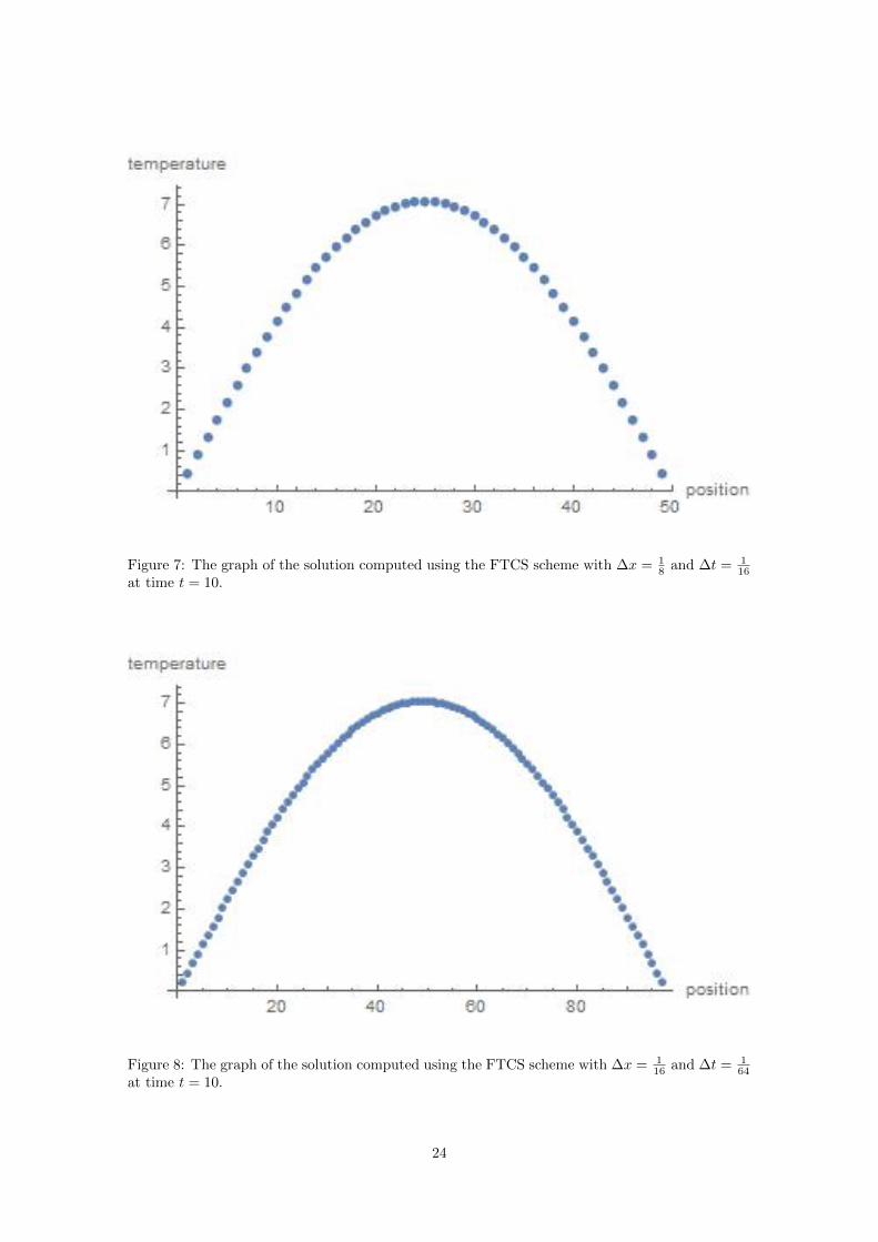
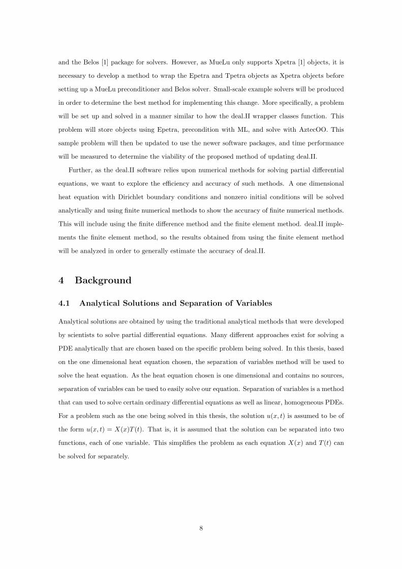
Figure 7: The graph of the solution computed using the FTCS scheme with ∆x = 18 and ∆t = 1
16at time t = 10.
Figure 8: The graph of the solution computed using the FTCS scheme with ∆x = 116 and ∆t = 1
64at time t = 10.
24

Figure 9: The graph of the solution computed using the FTCS scheme with ∆x = 132 and ∆t = 1
256at time t = 10.
Figure 10: The graph of the solution computed using the FTCS scheme with ∆x = 164 and
∆t = 11024 at time t = 10.
25

Figure 11: The graph compares the values of the analytical solution and the values of the solutionobtained using the finite difference method at x = 3 and t = 10, i.e. u(3, 10). The constant lineis the value obtained from the analytical solution and the line decreasing in value corresponds tothe values obtained from the finite difference method for decreasing ∆x.
26

Table 1: Results of Finite Difference∆x ∆t u(3, 10)
1 1 7.1165312 1 7.0833114
14 7.08334
18
116 7.06539
116
164 7.05089
132
1256 7.04207
164
11024 7.03723
Analytical - 7.03211
Having verified the analytical solution to the one dimensional heat equation, the accuracy
of the FTCS scheme of the finite difference method can be analyzed. Figures 4-10 show that
as both the number of time steps and the number of points on the problem space increase, the
approximation of the method converges to the analytical solution. It should be noted that this
method does not maintain zero temperature at the endpoints. However, as the problem is further
discretized, the end point values do tend back towards zero. Figure 11 shows this convergence by
plotting the values for u(3, 10) obtained from FTCS scheme against the value obtained from the
analytical solution. While the approximation achieved at ∆x = 164 and ∆t = 1
1024 is very close to
the analytical solution (roughly .05 off), it was not possible to further refine the problem and get a
better approximation without causing the Mathematica software to crash. Thus, while the FTCS
scheme of the finite difference method is simple and easy to implement, it is not a realistic method
when either a large problem is being solved or when a very close approximation is required.
27

6.1.3 Finite Element Method Results
Figure 12: The graph compares the values of the analytical solution and the values of the solutionobtained using the Crank Nicolson finite element method at x = 3 and t = 10, i.e. u(3, 10). Thesolutions are obtained from the Matlab implementation of this method. The constant line is thevalue obtained from the analytical solution and the line decreasing in value corresponds to thevalues obtained from the finite element method for decreasing ∆x.
28

Table 2: Results of Finite Element Method∆x ∆t u(3, 10)
1 1 7.0591112 1 7.039614
14 7.0340
18
116 7.0326
116
164 7.0322
132
1256 7.0321
164
11024 7.0321
Analytical - 7.03211
Figure 13: The graph compares the value of the analytical solution, the values of the solutionobtained using the Crank Nicolson finite element method, and the values of the solution obtainedusing the FTCS finite difference scheme at x = 3 and t = 10, i.e. u(3, 10). The solutions fromthe finite element method are obtained from the Matlab implementation of this method. Theconstant line is the value obtained from the analytical solution and the line decreasing in valuecorresponds to the values obtained from the finite element method for decreasing ∆x.
29

When looking at the results of the Crank-Nicolson scheme of the finite element method, specif-
ically Figure 13, it becomes clear that this method provides a much better approximation than
the finite difference approach. It converged to the solution much more quickly than the finite
difference method did. A coarser discretization of the problem was able to produce much better
results for u(3, 10) than the same discretization using FTCS. As a result, the Crank-Nicolson
scheme of the finite element method appears to be an adequate choice for problems where close
approximations are required.
6.2 Small Scale Example Results
Figure 14: A scatterplot of 10 time trials for MLAztecOO.cpp, MLBelos.cpp, and MueLuBelos.cppwith a problem size of 503. The measured time is total time to run including problem setup andsolving. This plot shows the range in time performance for each file and the comparative time tocomplete between each file.
30

Figure 15: A scatterplot of 10 time trials for MLAztecOO.cpp, MLBelos.cpp, and MueLuBelos.cppwith a problem size of 503. The measured time is the amount of time taken to solve the problem.Time to setup is not included. This plot shows the range in solving time performance for each fileand the comparative time to solve between each file.
Figure 16: A scatterplot of 10 time trials for MLAztecOO.cpp, MLBelos.cpp, and MueLuBelos.cppwith a problem size of 1203. The measured time is total time to run including problem setup andsolving. This plot shows the range in time performance for each file and the comparative time tocomplete between each file.
31
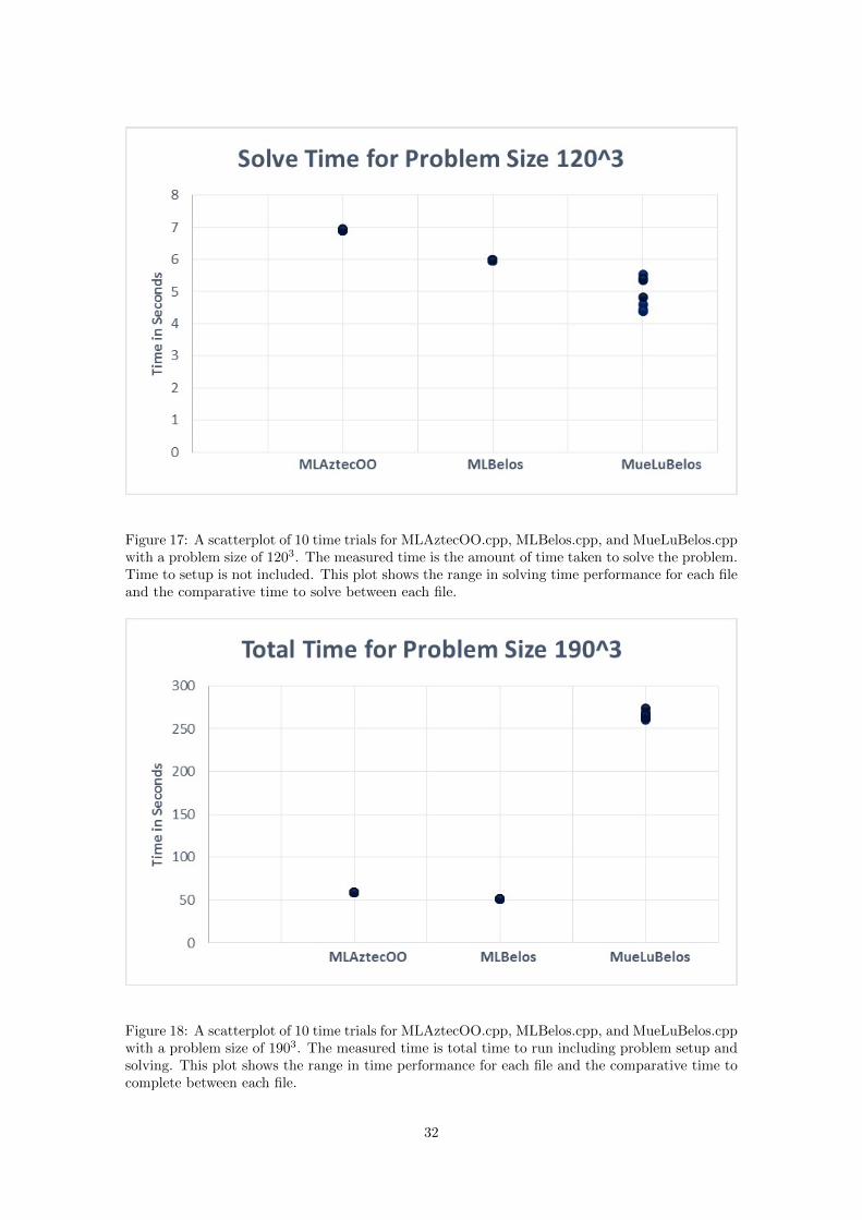
Figure 17: A scatterplot of 10 time trials for MLAztecOO.cpp, MLBelos.cpp, and MueLuBelos.cppwith a problem size of 1203. The measured time is the amount of time taken to solve the problem.Time to setup is not included. This plot shows the range in solving time performance for each fileand the comparative time to solve between each file.
Figure 18: A scatterplot of 10 time trials for MLAztecOO.cpp, MLBelos.cpp, and MueLuBelos.cppwith a problem size of 1903. The measured time is total time to run including problem setup andsolving. This plot shows the range in time performance for each file and the comparative time tocomplete between each file.
32

Figure 19: A scatterplot of 10 time trials for MLAztecOO.cpp, MLBelos.cpp, and MueLuBelos.cppwith a problem size of 1903. The measured time is the amount of time taken to solve the problem.Time to setup is not included. This plot shows the range in solving time performance for each fileand the comparative time to solve between each file.
Figure 20: A scatterplot of 10 time trials for MLAztecOO.cpp, MLBelos.cpp, and MueLuBelos.cppwith a problem size of 2603. The measured time is total time to run including problem setup andsolving. This plot shows the range in time performance for each file and the comparative time tocomplete between each file.
33

Figure 21: A scatterplot of 10 time trials for MLAztecOO.cpp, MLBelos.cpp, and MueLuBelos.cppwith a problem size of 2603. The measured time is the amount of time taken to solve the problem.Time to setup is not included. This plot shows the range in solving time performance for each fileand the comparative time to solve between each file.
Figure 22: A scatterplot of 10 time trials for MLAztecOO.cpp, MLBelos.cpp, and MueLuBelos.cppwith a problem size of 3303. The measured time is total time to run including problem setup andsolving. This plot shows the range in time performance for each file and the comparative time tocomplete between each file.
34

Figure 23: A scatterplot of 10 time trials for MLAztecOO.cpp, MLBelos.cpp, and MueLuBelos.cppwith a problem size of 3303. The measured time is the amount of time taken to solve the problem.Time to setup is not included. This plot shows the range in solving time performance for each fileand the comparative time to solve between each file.
Figure 24: A scatterplot of 10 time trials for MLAztecOO.cpp, MLBelos.cpp, and MueLuBelos.cppwith a problem size of 4003. The measured time is total time to run including problem setup andsolving. This plot shows the range in time performance for each file and the comparative time tocomplete between each file.
35

Figure 25: A scatterplot of 10 time trials for MLAztecOO.cpp, MLBelos.cpp, and MueLuBelos.cppwith a problem size of 4003. The measured time is the amount of time taken to solve the problem.Time to setup is not included. This plot shows the range in solving time performance for each fileand the comparative time to solve between each file.
36

Next, we analyze the results of the proposed method of updating the deal.II software. Overall,
there is a trend of Belos performing slightly better as a solver than AztecOO. Further, MueLu
paired with Belos on every problem size performed better than the other two implementations in
terms of solving time. This trend can especially be seen in Figures 15, 17, 19, and 25. ML with
AztecOO and ML with Belos performed very similarly concerning both solve time and total time.
In general there was a trend of ML with Belos performing slightly better than ML with AztecOO
in terms of both solving and total time. However, Figures 21, 23 ,24, and 25 show some instances
in which ML with AztecOO performed better than ML with Belos on certain runs. These results
are in line with what was expected. However, concerning total time, MueLu paired with Belos took
almost five times as long to complete as either of the other two implementations. When looking at
the source code it became clear what was causing the significant increase in time. The translation
of the Epetra matrix to an Xpetra object (lines 104-110 of MueLuBelos.cpp in Appendix) is being
executed one row at a time in a for loop. As the problem sizes increase, this very quickly becomes
an issue. Some form of parallelism or a better method needs to be implemented to resolve this
issue before deal.II can realistically implement the proposed method of integrating MueLu into its
software.
7 Conclusion
1. Performance of Finite Methods
This work confirmed that finite numerical methods find adequate approximations to tradi-
tional analytical solutions to differential equations. Further, it can be noted that the finite
difference, forward in time scheme is not the most efficient method as the number of time
steps required rapidly increases as the discretization of the problem space becomes more re-
fined. This results in The finite element method using the Crank-Nicolson System converged
to the analytical solution much more quickly than the finite difference method and was able
to give a better approximation with a coarser discretization of the problem space than was
achieved using the finite difference method.
2. Proposed Method of Updating the deal.II Software
While, the small scale examples showed decrease in performance for total time when uti-
lizing MueLu over ML, I predict that with added parallelism in the set up phase and with
larger, more complex examples, time performance will increase. There is currently too much
overhead created by translating the objects into Xpetra objects. Specifically, I believe that
37

the current method of transferring the values of the matrix one row at a time is contributing
the most to the total run time. Looking at just the time used for solving the problem shows
that MueLu combined with Belos does perform better than ML and AztecOO together or
ML and Belos together.
This thesis explored methods of solving partial differential equations that can be implemented
with a computer. As computers cannot handle infinite amounts of points on a solution, it is
necessary to discretize the solution space and solve using a finite numerical method. This work
was able to show the accuracy of several such methods on the one-dimensional heat equation with
Dirichlet boundary conditions. Further, a method of updating the deal.II software was proposed
and its potential benefits were explored by analyzing time performance on small scale examples.
7.1 Future Work
In the future, a method should be developed for decreasing the overhead time created from trans-
lating the Epetra matrix to an Xpetra matrix. As the computation inside the current for loop
accomplishing this transition is independent, I believe that this could easily be parallelized in
order to increase performance. Further, if a parallel or distributed method were implemented in
the Xpetra class to translate Epetra or Tpetra matrices, I believe that even better performance
could be seen.
The next step along this course of work would be to implement the suggested changes in
the deal.II software. As shown in the small scale examples, the code needs to be written so as
to encapsulate or wrap the existing objects as Xpetra objects so that they are compatible with
MueLu preconditioners. As hardware improves in accordance with Moore’s Law, it is important to
focus on maintaining and improving software as new technologies emerge and hardware improves.
38

References
[1] The trilinos project. trilinos.org. both documentation of and source code for the Trilinos
Project.
[2] W. Bangerth, T. Heister, L. Heltai, G. Kanschat, M. Kronbichler, M. Maier, B. Turcksin,
and T. D. Young. The deal.ii library, version 8.1. arXiv preprint, http: // arxiv. org/ abs/
1312. 2266v4 , 2013.
[3] John R. Cannon. The One-Dimensional Heat Equation. Addison-Wesley Publishing Com-
pany, Inc., 1984.
[4] D. DeTurck. Math 241: Solving the heat equation. 2012. Course notes for Math 241 at
University of Pennsylvania.
[5] Gene H. Golub and Charles F. Van Loan. Matrix Computations. John Hopkins University
Press, 2012.
[6] G. Recktenwald. Heatcn.m. Matlab code implementing the Crank-Nicolson scheme for solving
the 1D heat equation.
[7] G. Recktenwald. Finite-difference approximations to the heat equation. 2011.
[8] Yousef Saad. Iterative Methods for Sparse Linear Systems. Society for Industrial and Applied
Mathematics, 2003.
[9] P. Seshaiyar. Finite-difference method for the 1d heat equation. 2012. Course notes for
Math679 at George Mason University.
[10] Griffiths D.V. Margetts L. Smith, I.M. Programming the Finite Element Method. John Wiley
& Sons, 2013.
[11] R. Vichnevetsky. Computer Methods for Partial Differential Equations, Volume 1. Prentice-
Hall, Inc., 1981.
[12] Taylor R. L. Zhu J. Z. Zienkiewicz, O. C. Finite Element Method : Its Basis and Fundamen-
tals. Butterworth-Heinemann, 2005.
39

8 Appendix
8.1 Computing Architecture
Each node of Melchior consists of 12 cores each with 2 threads. Each thread state can be defined
as follows:
1 Mel Nodes 0 , 1 , 2 , 4 , 5 , 6 , 7
2
3 p ro c e s s o r : 23
4 vendor id : GenuineInte l
5 cpu fami ly : 6
6 model : 45
7 model name : I n t e l (R) Xeon(R) CPU E5−2420 0 @ 1.90GHz
8 stepp ing : 7
9 microcode : 1808
10 cpu MHz : 1200.000
11 cache s i z e : 15360 KB
12 phy s i c a l id : 1
13 s i b l i n g s : 12
14 core id : 5
15 cpu co r e s : 6
16 ap i c i d : 43
17 i n i t i a l ap i c i d : 43
18 fpu : yes
19 fpu excep t i on : yes
20 cpuid l e v e l : 13
21 wp : yes
22 f l a g s : fpu vme de pse t s c msr pae mce cx8 ap ic sep mtrr pge mca cmov pat
pse36 c l f l u s h dts acp i mmx f x s r s s e s s e2 s s ht tm pbe s y s c a l l nx pdpe1gb
rdtscp lm con s t an t t s c arch perfmon pebs bts rep good xtopology nons top t s c
aper fmper f pni pclmulqdq dtes64 monitor d s cp l vmx smx e s t tm2 s s s e 3 cx16 xtpr
pdcm pcid dca s s e 4 1 s s e 4 2 x2apic popcnt t s c d e ad l i n e t ime r aes xsave avx
l ah f lm ida arat epb xsaveopt pln pts dts tpr shadow vnmi f l e x p r i o r i t y ept vpid
23 bogomips : 3793.04
24 c l f l u s h s i z e : 64
25 cache a l ignment : 64
26 address s i z e s : 46 b i t s phys i ca l , 48 b i t s v i r t u a l
27 power management :
8.2 MLAztecOO.cpp Source Code
40

1 /∗
2 ∗ MLAztecOO. cpp
3 ∗ Taken from Tr i l i n o s t u t o r i a l at https : // code . goog l e . com/p/ t r i l i n o s /wik i /MLAztecOO
4 ∗
5 ∗/
6
7 //
8 // Use ML to bu i ld a smoothed aggregat i on mu l t i g r id operator .
9 // Use the operator as a black−box p r e cond i t i on e r in AztecOO ’ s CG.
10 //
11 #inc lude ”Epetra Conf igDefs . h”
12 #i f d e f HAVE MPI
13 # inc lude ”mpi . h”
14 # inc lude ”Epetra MpiComm . h”
15 #e l s e
16 # inc lude ”Epetra SerialComm . h”
17 #end i f
18 #inc lude ”Epetra Map . h”
19 #inc lude ”Epetra Vector . h”
20 #inc lude ”Epetra RowMatrix . h”
21 #inc lude ”Epetra CrsMatrix . h”
22 #inc lude ”Epetra LinearProblem . h”
23 #inc lude ”Epetra Time . h”
24 #inc lude ”AztecOO . h”
25
26 // The ML inc lude f i l e r equ i r ed when working with Epetra ob j e c t s .
27 #inc lude ”m l epe t r a p r e c ond i t i on e r . h”
28
29 #inc lude ” Tr i l i n o s Ut i l C r sMat r i xGa l l e r y . h”
30
31 us ing namespace Teuchos ;
32 us ing namespace T r i l i n o s U t i l ;
33 us ing namespace std ;
34
35 #inc lude <iostream>
36 #inc lude <sys / time . h>
37 #inc lude <time . h>
38
39 i n t
40 main ( i n t argc , char ∗argv [ ] )
41 {
42
41

43 s t r u c t t imeva l tim ;
44 gett imeofday(&tim , NULL) ;
45 double t1=tim . t v s e c+(tim . tv us e c /1000000 .0) ;
46
47
48 #i f d e f EPETRA MPI
49 MPI Init (&argc ,&argv ) ;
50 Epetra MpiComm Comm (MPICOMMWORLD) ;
51 #e l s e
52 Epetra SerialComm Comm;
53 #end i f
54
55 Epetra Time Time(Comm) ;
56
57 // I n i t i a l i z e a Gal l e ry object , f o r gene ra t ing a 3−D Laplac ian
58 // matrix d i s t r i b u t e d over the g iven communicator Comm.
59 CrsMatr ixGal lery Gal l e ry ( ” l ap l a c e 3d ” , Comm) ;
60
61 Gal l e ry . Set ( ” prob l em s i z e ” , 1728000) ;
62
63 // Get po i n t e r s to the generated matrix and a t e s t l i n e a r problem .
64 Epetra RowMatrix∗ A = Gal l e ry . GetMatrix ( ) ;
65
66 Epetra LinearProblem ∗ Problem = Gal l e ry . GetLinearProblem ( ) ;
67
68 // Construct an AztecOO so l v e r ob j e c t f o r t h i s problem .
69 AztecOO so l v e r (∗Problem ) ;
70
71 // Create the p r e c ond i t i on e r ob j e c t and compute the mu l t i l e v e l h i e ra r chy .
72 ML Epetra : : Mu l t iLeve lPrecond i t i one r ∗ MLPrec =
73 new ML Epetra : : Mu l t iLeve lPrecond i t i one r (∗A, true ) ;
74
75 // Te l l AztecOO to use t h i s p r e c ond i t i on e r .
76 s o l v e r . SetPrecOperator (MLPrec) ;
77
78 // Te l l AztecOO to use CG to so l v e the problem .
79 s o l v e r . SetAztecOption ( AZ solver , AZ cg ) ;
80
81 // Te l l AztecOO to output s t a tu s in fo rmat ion every i t e r a t i o n
82 // ( hence the 1 , which i s the output f requency in terms o f
83 // number o f i t e r a t i o n s ) .
84 s o l v e r . SetAztecOption (AZ output , 1) ;
42

85
86 // Maximum number o f i t e r a t i o n s to t ry .
87 i n t N i t e r s = 150 ;
88 // Convergence t o l e r an c e .
89 double t o l = 1e−10;
90
91 // g e t t i n g time a f t e r s e t t i n g up problem
92 gett imeofday(&tim , NULL) ;
93 double t2=tim . t v s e c+(tim . tv us e c /1000000 .0) ;
94
95 // Solve the l i n e a r problem .
96 s o l v e r . I t e r a t e ( Niters , t o l ) ;
97
98 // g e t t i n g time a f t e r s o l v e r completes
99 gett imeofday(&tim , NULL) ;
100 double t3=tim . t v s e c+(tim . tv us e c /1000000 .0) ;
101
102 // Pr int out some in fo rmat ion about the p r e c ond i t i on e r
103 i f (Comm.MyPID( ) == 0)
104 cout << MLPrec−>GetOutputList ( ) ;
105
106 // We’ re done with the p r e cond i t i on e r now , so we can d e a l l o c a t e i t .
107 d e l e t e MLPrec ;
108
109 // Ver i f y the s o l u t i o n by computing the r e s i d u a l e x p l i c i t l y .
110 double r e s i d u a l = 0 . 0 ;
111 double d i f f = 0 . 0 ;
112 Gal l e ry . ComputeResidual (& r e s i d u a l ) ;
113 Gal l e ry . ComputeDiffBetweenStartingAndExactSolutions (& d i f f ) ;
114
115 // The Epetra Time ob j e c t has been keeping t rack o f e l apsed time
116 // l o c a l l y ( on t h i s MPI proce s s ) . Take the min and max g l o b a l l y
117 // to f i nd the min and max e lapsed time over a l l MPI p ro c e s s e s .
118 double myElapsedTime = Time . ElapsedTime ( ) ;
119 double minElapsedTime = 0 . 0 ;
120 double maxElapsedTime = 0 . 0 ;
121 ( void ) Comm. MinAll (&myElapsedTime , &minElapsedTime , 1) ;
122 ( void ) Comm.MaxAll (&myElapsedTime , &maxElapsedTime , 1) ;
123
124 i f (Comm.MyPID( )==0) {
125 const i n t numProcs = Comm.NumProc ( ) ;
126 cout << ” | | b−Ax | | 2 = ” << r e s i d u a l << endl
43

127 << ” | | x exact − x | | 2 = ” << d i f f << endl
128 << ”Min t o t a l time ( s ) over ” << numProcs << ” p r o c e s s e s : ”
129 << minElapsedTime << endl
130 << ”Max t o t a l time ( s ) over ” << numProcs << ” p r o c e s s e s : ”
131 << maxElapsedTime << endl ;
132 }
133
134 // p r i n t i n g out time data
135 cout << t3−t1 << ” seconds e lapsed ” << endl ;
136 cout << t3−t2 << ” seconds e lapsed s o l v i n g ” << endl ;
137
138 #i f d e f EPETRA MPI
139 MPI Final ize ( ) ;
140 #end i f
141 re turn (EXIT SUCCESS) ;
142 }
8.3 MLBelos.cpp Source Code
1 /∗
2 ∗ MLBelos . cpp
3 ∗ by Emily Furst
4 ∗ Modif ied from o r i g i n a l T r i l i n o s t u t o r i a l at https : // code . goog l e . com/p/ t r i l i n o s /
wik i /MLAztecOO
5 ∗
6 ∗/
7
8 //
9 // Use ML to bu i ld a smoothed aggregat i on mu l t i g r id operator .
10 // Use Belos as a s o l v e r
11 //
12 #inc lude ”Epetra Conf igDefs . h”
13 #i f d e f HAVE MPI
14 # inc lude ”mpi . h”
15 # inc lude ”Epetra MpiComm . h”
16 #e l s e
17 # inc lude ”Epetra SerialComm . h”
18 #end i f
19 #inc lude ”Epetra Map . h”
20 #inc lude ”Epetra Vector . h”
21 #inc lude ”Epetra RowMatrix . h”
22 #inc lude ”Epetra CrsMatrix . h”
44

23 #inc lude ”Epetra LinearProblem . h”
24 #inc lude ”Epetra Time . h”
25 #inc lude ”AztecOO . h”
26 #inc lude ”Teuchos ParameterList . hpp”
27 #inc lude ”Teuchos RCP . hpp”
28 #inc lude ”BelosLinearProblem . hpp”
29 #inc lude ”BelosBlockCGSolMgr . hpp”
30 #inc lude ”BelosEpetraAdapter . hpp”
31 #inc lude ”MueLu . hpp”
32
33
34 // The ML inc lude f i l e r equ i r ed when working with Epetra ob j e c t s .
35 #inc lude ”m l epe t r a p r e c ond i t i on e r . h”
36
37 #inc lude ” Tr i l i n o s Ut i l C r sMat r i xGa l l e r y . h”
38
39 us ing namespace Teuchos ;
40 us ing namespace T r i l i n o s U t i l ;
41 us ing namespace std ;
42
43 #inc lude <iostream>
44 #inc lude <sys / time . h>
45 #inc lude <time . h>
46
47 i n t
48 main ( i n t argc , char ∗argv [ ] )
49 {
50
51 s t r u c t t imeva l tim ;
52 gett imeofday(&tim , NULL) ;
53 double t1=tim . t v s e c+(tim . tv us e c /1000000 .0) ;
54
55
56 #i f d e f EPETRA MPI
57 MPI Init (&argc ,&argv ) ;
58 Epetra MpiComm Comm (MPICOMMWORLD) ;
59 #e l s e
60 Epetra SerialComm Comm;
61 #end i f
62
63 Epetra Time Time(Comm) ;
64
45

65 // I n i t i a l i z e a Gal l e ry object , f o r gene ra t ing a 3−D Laplac ian
66 // matrix d i s t r i b u t e d over the g iven communicator Comm.
67 CrsMatr ixGal lery Gal l e ry ( ” l ap l a c e 3d ” , Comm) ;
68
69 //problem s i z e must be a p e r f e c t cube
70 Gal l e ry . Set ( ” prob l em s i z e ” , 1728000) ;
71
72 // Get po i n t e r s to the generated matrix and a t e s t l i n e a r problem .
73
74 RCP<Epetra RowMatrix> A = rcp ( Gal l e ry . GetMatrix ( ) , f a l s e ) ;
75
76 RCP<Epetra Mult iVector> LHS = rcp ( Gal l e ry . GetLinearProblem ( )−>GetLHS( ) , f a l s e ) ;
77 RCP<Epetra Mult iVector> RHS = rcp ( Gal l e ry . GetLinearProblem ( )−>GetRHS( ) , f a l s e ) ;
78
79
80
81
82 typede f Epetra Mult iVector MV;
83 typede f Epetra Operator OP;
84
85 RCP<Belos : : LinearProblem<double ,MV,OP> > problem = rcp (new Belos : : LinearProblem<
double ,MV,OP>(A, LHS, RHS) ) ;
86
87 bool s e t = problem−>setProblem ( ) ;
88 TEUCHOS TEST FOR EXCEPTION( ! set ,
89 std : : runt ime er ror ,
90 ”∗∗∗ Belos : : LinearProblem f a i l e d to s e t up c o r r e c t l y ! ∗∗∗” ) ;
91
92
93 // Create the p r e c ond i t i on e r ob j e c t and compute the mu l t i l e v e l h i e ra r chy .
94 ML Epetra : : Mu l t iLeve lPrecond i t i one r ∗ MLPrec =
95 new ML Epetra : : Mu l t iLeve lPrecond i t i one r (∗A, true ) ;
96
97 //Begin to s e t up Belos s o l v e r
98
99 RCP<Belos : : EpetraPrecOp> prec = rcp (new Belos : : EpetraPrecOp ( rcp (MLPrec , f a l s e ) ) ) ;
100 problem−>setRightPrec ( prec ) ;
101
102
103 RCP<ParameterList> b e l o sL i s t = rcp (new ParameterList ( ) ) ;
104 be l o sL i s t−>s e t ( ”Block S i z e ” , 1) ; // B lo ck s i z e to be used by
i t e r a t i v e s o l v e r
46

105 be l o sL i s t−>s e t ( ”Maximum I t e r a t i o n s ” , 150) ; // Maximum number o f i t e r a t i o n s
a l lowed
106 be l o sL i s t−>s e t ( ”Convergence Tolerance ” , 1e−10) ; // Re la t i v e convergence t o l e r an c e
reques ted
107 be l o sL i s t−>s e t ( ”Verbos i ty ” , Belos : : Errors+Belos : : Warnings+Belos : : TimingDetai l s+
Belos : : FinalSummary+Belos : : S ta tu sTes tDeta i l s+Belos : : I t e r a t i o nD e t a i l s ) ;
108
109
110
111 Belos : : BlockCGSolMgr<double ,MV,OP> be l o sSo l v e r ( problem , b e l o sL i s t ) ;
112
113
114 // r e t r i e v e time be f o r e s o l v e r computes and a f t e r setup
115 gett imeofday(&tim , NULL) ;
116 double t2=tim . t v s e c+(tim . tv us e c /1000000 .0) ;
117
118
119 //Belos s o l v e r s o l v e s problem
120 Belos : : ReturnType r e t = be l o sSo l v e r . s o l v e ( ) ;
121
122
123 // r e t r i e v e time a f t e r s o l v i n g completed
124 gett imeofday(&tim , NULL) ;
125 double t3=tim . t v s e c+(tim . tv us e c /1000000 .0) ;
126
127
128 // We’ re done with the p r e cond i t i on e r now , so we can d e a l l o c a t e i t .
129 d e l e t e MLPrec ;
130
131 // Ver i f y the s o l u t i o n by computing the r e s i d u a l e x p l i c i t l y .
132 double r e s i d u a l = 0 . 0 ;
133 double d i f f = 0 . 0 ;
134 Gal l e ry . ComputeResidual (& r e s i d u a l ) ;
135 Gal l e ry . ComputeDiffBetweenStartingAndExactSolutions (& d i f f ) ;
136
137 // The Epetra Time ob j e c t has been keeping t rack o f e l apsed time
138 // l o c a l l y ( on t h i s MPI proce s s ) . Take the min and max g l o b a l l y
139 // to f i nd the min and max e lapsed time over a l l MPI p ro c e s s e s .
140 double myElapsedTime = Time . ElapsedTime ( ) ;
141 double minElapsedTime = 0 . 0 ;
142 double maxElapsedTime = 0 . 0 ;
143 ( void ) Comm. MinAll (&myElapsedTime , &minElapsedTime , 1) ;
47

144 ( void ) Comm.MaxAll (&myElapsedTime , &maxElapsedTime , 1) ;
145
146 cout<<endl ;
147
148 cout << ”Parameter L i s t : ” << ∗ b e l o sL i s t <<endl ;
149
150 i f (Comm.MyPID( )==0) {
151 const i n t numProcs = Comm.NumProc ( ) ;
152 cout << ” | | b−Ax | | 2 = ” << r e s i d u a l << endl
153 << ” | | x exact − x | | 2 = ” << d i f f << endl
154 << ”Min t o t a l time ( s ) over ” << numProcs << ” p r o c e s s e s : ”
155 << minElapsedTime << endl
156 << ”Max t o t a l time ( s ) over ” << numProcs << ” p r o c e s s e s : ”
157 << maxElapsedTime << endl ;
158 i f ( r e t == Belos : : Converged ) {
159 std : : cout << ”Belos converged . ” << std : : endl ;
160 } e l s e {
161 std : : cout << ”Belos did not converge . ” << std : : endl ;
162 }
163 }
164
165
166 cout << t3−t1 << ” seconds e lapsed ” << endl ;
167 cout << t3−t2 << ” seconds e lapsed s o l v i n g ” << endl ;
168
169 #i f d e f EPETRA MPI
170
171 MPI Final ize ( ) ;
172 #end i f
173
174 re turn (EXIT SUCCESS) ;
175 }
8.4 MueLuBelos.cpp Source Code
1 /∗
2 ∗ MueLuBelos . cpp
3 ∗ by Emily Furst
4 ∗ Modif ied from MLBelos . cpp and o r i g i n a l T r i l i n o s t u t o r i a l at https : // code . goog l e .
com/p/ t r i l i n o s /wik i /MLAztecOO
5 ∗
6 ∗/
48

7
8 //
9 //Use MueLu pr e cond i t i on e r with Belos s o l v e r to s o l v e problem se t up
10 //
11 #inc lude ”Epetra Conf igDefs . h”
12 #i f d e f HAVE MPI
13 # inc lude ”mpi . h”
14 # inc lude ”Epetra MpiComm . h”
15 #e l s e
16 # inc lude ”Epetra SerialComm . h”
17 #end i f
18 #inc lude ”Epetra Map . h”
19 #inc lude ”Epetra Vector . h”
20 #inc lude ”Epetra RowMatrix . h”
21 #inc lude ”Epetra CrsMatrix . h”
22 #inc lude ”Epetra LinearProblem . h”
23 #inc lude ”Epetra Time . h”
24 #inc lude ”Teuchos ParameterList . hpp”
25 #inc lude ”Teuchos RCP . hpp”
26 #inc lude ”BelosLinearProblem . hpp”
27 #inc lude ”BelosBlockCGSolMgr . hpp”
28 #inc lude ”BelosEpetraAdapter . hpp”
29 #inc lude ”MueLu . hpp”
30 #inc lude ”Xpetra Vector . hpp”
31 #inc lude ”Xpetra RowMatrix . hpp”
32 #inc lude ”Xpetra CrsMatrix . hpp”
33 #inc lude ”Xpetra EpetraCrsMatrix . hpp”
34
35 #inc lude <iostream>
36
37 #inc lude <Xpetra Mult iVectorFactory . hpp>
38
39
40 #inc lude <MueLu Tril inosSmoother . hpp> //TODO: remove
41
42 // Header f i l e s d e f i n i n g d e f au l t types f o r template parameters .
43 // These headers must be inc luded a f t e r other MueLu/Xpetra headers .
44 #inc lude <MueLu UseDefaultTypes . hpp> // => Sca la r=double , Loca lOrdina l=int ,
GlobalOrdinal=in t
45
46 #inc lude <BelosConf igDefs . hpp>
47 #inc lude <BelosLinearProblem . hpp>
49
48 #inc lude <BelosBlockCGSolMgr . hpp>
49 #inc lude <BelosXpetraAdapter . hpp> // => This header d e f i n e s Belos : : XpetraOp
50 #inc lude <BelosMueLuAdapter . hpp> // => This header d e f i n e s Belos : : MueLuOp
51
52
53 // The ML inc lude f i l e r equ i r ed when working with Epetra ob j e c t s .
54 #inc lude ”m l epe t r a p r e c ond i t i on e r . h”
55
56 #inc lude ” Tr i l i n o s Ut i l C r sMat r i xGa l l e r y . h”
57
58 us ing namespace Teuchos ;
59 us ing namespace T r i l i n o s U t i l ;
60 us ing namespace std ;
61 us ing namespace Xpetra ;
62 us ing namespace MueLu ;
63
64 #inc lude <iostream>
65 #inc lude <sys / time . h>
66 #inc lude <time . h>
67
68 i n t
69 main ( i n t argc , char ∗argv [ ] )
70 {
71
72 s t r u c t t imeva l tim ;
73 gett imeofday(&tim , NULL) ;
74 double t1=tim . t v s e c+(tim . tv us e c /1000000 .0) ;
75
76 #inc lude <MueLu UseShortNames . hpp>
77
78 #i f d e f EPETRA MPI
79 MPI Init (&argc ,&argv ) ;
80 Epetra MpiComm Comm (MPICOMMWORLD) ;
81 #e l s e
82 Epetra SerialComm Comm;
83 #end i f
84
85 Epetra Time Time(Comm) ;
86
87 // I n i t i a l i z e a Gal l e ry object , f o r gene ra t ing a 3−D Laplac ian
88 // matrix d i s t r i b u t e d over the g iven communicator Comm.
89 CrsMatr ixGal lery Gal l e ry ( ” l ap l a c e 3d ” , Comm) ;
50

90
91 //problem s i z e must be a p e r f e c t cube as working with 3−D Laplac ian
92 Gal l e ry . Set ( ” prob l em s i z e ” , 125000) ;
93
94 // Get po i n t e r s to the generated matrix and a t e s t l i n e a r problem .
95 Epetra CrsMatrix A = ∗( Ga l l e ry . GetMatrix ( ) ) ;
96 Epetra CrsGraph graphA = A. Graph ( ) ;
97
98 // convert Epetra Matrix to Xpetra Matrix ob j e c t
99
100 RCP<const CrsGraph > rgraphA = toXpetra<int >(graphA ) ;
101 RCP<Matrix > rA = rcp (new CrsMatrixWrap ( rgraphA ) ) ;
102 rA−>s e tA l lToSca la r (0 ) ;
103 rA−>r e sumeFi l l ( ) ;
104 f o r ( i n t i = 0 ; i < A. NumGlobalRows ( ) ; i++){
105 i n t num = 0 , ∗ i n d i c e s = new in t [A. NumGlobalEntries ( i ) ] ;
106 double ∗ va lue s = new double [A. NumGlobalEntries ( i ) ] ;
107 A. ExtractGlobalRowCopy ( i , A. NumGlobalCols ( ) ,num, values , i n d i c e s ) ;
108
109 rA−>r ep laceGloba lVa lues ( i , arrayView<const int >( i nd i c e s , num) , arrayView<const
double>(values , num) ) ;
110 }
111 rA−>f i l lComp l e t e ( ) ;
112
113 // r e t r i e v e LHS and RHS vec to r s
114
115 Epetra LinearProblem ∗ Problem = Gal l e ry . GetLinearProblem ( ) ;
116 RCP<Epetra Mult iVector> LHS = rcp (Problem−>GetLHS( ) , f a l s e ) ;
117 RCP<Epetra Mult iVector> RHS = rcp (Problem−>GetRHS( ) , f a l s e ) ;
118
119 // convert LHS and RHS Epetra ve c to r s to Xpetra ob j e c t s
120
121 RCP<MultiVector > rLHS = toXpetra<int >(LHS) ;
122 RCP<MultiVector > rRHS = toXpetra<int >(RHS) ;
123
124
125 // s e t t i n g up MueLu pr e cond i t i on e r and Belos s o l v e r s
126 FactoryManager M;
127
128 RCP<Hierarchy> H = rcp (new Hierarchy ( rA) ) ;
129
130 H−>setVerbLeve l ( Teuchos : : VERB HIGH) ;
51

131
132 RCP<Factory> AcFact = rcp (new RAPFactory ( ) ) ;
133 M. SetFactory ( ”A” , AcFact ) ;
134
135
136 H−>Setup (M) ;
137
138 typede f Mult iVector MV;
139 typede f Belos : : OperatorT<MV> OP;
140
141 RCP<OP> belosOp = rcp (new Belos : : XpetraOp<SC, LO, GO, NO>(rA) ) ;
142 RCP<OP> be lo sPrec = rcp (new Belos : : MueLuOp<SC, LO, GO, NO>(H) ) ;
143
144 RCP< Belos : : LinearProblem<SC, MV, OP> > belosProblem = rcp (new Belos : :
LinearProblem<SC, MV, OP>(belosOp , rLHS , rRHS) ) ;
145 belosProblem−>s e tLe f tPr e c ( be lo sPrec ) ;
146
147 bool s e t = belosProblem−>setProblem ( ) ;
148 TEUCHOS TEST FOR EXCEPTION( ! set ,
149 std : : runt ime er ror ,
150 ”∗∗∗ Belos : : LinearProblem f a i l e d to s e t up c o r r e c t l y ! ∗∗∗” ) ;
151 i n t maxIts = 150 ;
152 double t o l = 1e−10;
153 Teuchos : : ParameterList b e l o sL i s t ;
154 b e l o sL i s t . s e t ( ”Maximum I t e r a t i o n s ” , maxIts ) ; // Maximum number o f i t e r a t i o n s
a l lowed
155 b e l o sL i s t . s e t ( ”Convergence Tolerance ” , t o l ) ; // Re la t i v e convergence t o l e r an c e
reques ted
156 b e l o sL i s t . s e t ( ”Verbos i ty ” , Belos : : Errors + Belos : : Warnings + Belos : : TimingDetai l s
+ Belos : : S ta tu sTes tDeta i l s ) ;
157
158 // Create an i t e r a t i v e s o l v e r manager
159 RCP< Belos : : SolverManager<SC, MV, OP> > s o l v e r = rcp (new Belos : : BlockCGSolMgr<SC,
MV, OP>(belosProblem , rcp(&be l o sL i s t , f a l s e ) ) ) ;
160
161
162 // r e t r i e v e time a f t e r setup and be f o r e s o l v e
163 gett imeofday(&tim , NULL) ;
164 double t2=tim . t v s e c+(tim . tv us e c /1000000 .0) ;
165
166 // Perform so l v e
167
52

168 Belos : : ReturnType r e t = so lve r−>s o l v e ( ) ;
169
170 // r e t r i e v e time a f t e r s o l v e
171 gett imeofday(&tim , NULL) ;
172 double t3=tim . t v s e c+(tim . tv us e c /1000000 .0) ;
173
174 // Get the number o f i t e r a t i o n s f o r t h i s s o l v e .
175 std : : cout << ”Number o f i t e r a t i o n s performed f o r t h i s s o l v e : ” << so l ve r−>
getNumIters ( ) << std : : endl ;
176
177
178
179 // Ver i f y the s o l u t i o n by computing the r e s i d u a l e x p l i c i t l y .
180 double r e s i d u a l = 0 . 0 ;
181 double d i f f = 0 . 0 ;
182 Gal l e ry . ComputeResidual (& r e s i d u a l ) ;
183 Gal l e ry . ComputeDiffBetweenStartingAndExactSolutions (& d i f f ) ;
184
185 // The Epetra Time ob j e c t has been keeping t rack o f e l apsed time
186 // l o c a l l y ( on t h i s MPI proce s s ) . Take the min and max g l o b a l l y
187 // to f i nd the min and max e lapsed time over a l l MPI p ro c e s s e s .
188 double myElapsedTime = Time . ElapsedTime ( ) ;
189 double minElapsedTime = 0 . 0 ;
190 double maxElapsedTime = 0 . 0 ;
191 ( void ) Comm. MinAll (&myElapsedTime , &minElapsedTime , 1) ;
192 ( void ) Comm.MaxAll (&myElapsedTime , &maxElapsedTime , 1) ;
193
194 cout<<endl ;
195
196
197 i f (Comm.MyPID( )==0) {
198 const i n t numProcs = Comm.NumProc ( ) ;
199 cout << ” | | b−Ax | | 2 = ” << r e s i d u a l << endl
200 << ” | | x exact − x | | 2 = ” << d i f f << endl
201 << ”Min t o t a l time ( s ) over ” << numProcs << ” p r o c e s s e s : ”
202 << minElapsedTime << endl
203 << ”Max t o t a l time ( s ) over ” << numProcs << ” p r o c e s s e s : ”
204 << maxElapsedTime << endl ;
205 i f ( r e t == Belos : : Converged ) {
206 std : : cout << ”Belos converged . ” << std : : endl ;
207 } e l s e {
208 std : : cout << ”Belos did not converge . ” << std : : endl ;
53

209 }
210 }
211
212 // p r in t out time r e s u l t s
213 cout << t3−t1 << ” seconds e lapsed ” << endl ;
214 cout << t3−t2 << ” seconds e lapsed s o l v i n g ” << endl ;
215
216 #i f d e f EPETRA MPI
217
218 MPI Final ize ( ) ;
219 #end i f
220 re turn (EXIT SUCCESS) ;
221 }
8.5 Makefile for MLAztecOO.cpp
Note Makefiles for MLAztecOO.cpp, MLBelos.cpp, and MueLuBelos.cpp are essentially the same
with only the filename and executable name changed wherever they appear in the Makefile (lines
55,56,59,60).
1 # CMAKE F i l e f o r ”MyApp” app l i c a t i o n bu i l d i ng aga in s t an i n s t a l l e d T r i l i n o s
2
3 #This f i l e i s an adaptat ion o f the CMakeLists . txt f i l e that was converted from
4 #the bu i l dAga i n s tTr i l i n o s example . This Make f i l e was des igned to be used in a
5 #f l a t d i r e c t o r y s t r u c tu r e . I f you would l i k e to run t h i s example you w i l l need
6 #put t h i s f i l e and s r c f i l e . cpp , s r c f i l e . hpp , ma i n f i l e . cpp from
7 #bu i l dAga i n s tT r i l i n o s in to a new d i r e c t o r y . You w i l l then need to s e t the
8 #environment va r i ab l e MYAPP TRILINOS DIR to po int to your base i n s t a l l a t i o n o f
9 #Tr i l i n o s . Note that t h i s example assumes that the i n s t a l l a t i o n o f T r i l i n o s that
10 #you point to has Epetra enabled .
11
12 # Get T r i l i n o s as one en t i t y
13 inc lude $ (MYAPP TRILINOS DIR) inc lude /Make f i l e . export . T r i l i n o s
14
15 # Make sure to use same compi l e r s and f l a g s as T r i l i n o s
16 CXX=$ (Trilinos CXX COMPILER)
17 CC=$ (Trilinos C COMPILER)
18 FORT=$ (Trilinos Fortran COMPILER )
19
20 CXX FLAGS=$ (Trilinos CXX COMPILER FLAGS) $ (USER CXX FLAGS)
21 C FLAGS=$ (Trilinos C COMPILER FLAGS) $ (USERC FLAGS)
22 FORT FLAGS=$ (Trilinos Fortran COMPILER FLAGS ) $ (USER FORT FLAGS)
54

23
24 INCLUDE DIRS=$ (Trilinos INCLUDE DIRS ) $ (Trilinos TPL INCLUDE DIRS )
25 LIBRARY DIRS=$ (Trilinos LIBRARY DIRS ) $ (Trilinos TPL LIBRARY DIRS )
26 LIBRARIES=$ ( Trilinos LIBRARIES ) $ (Trilinos TPL LIBRARIES )
27
28 LINK FLAGS=$ (Trilinos EXTRA LD FLAGS)
29
30 #ju s t assuming that epet ra i s turned on .
31 DEFINES=−DMYAPPXPETRA
32 DEFINES=−DMYAPPEPETRA
33 DEFINES=−DMYAPPTPETRA
34 DEFINES=−DMYAPPGALERI
35 DEFINES=−DMYAPP STRATIMIKOS
36
37 de f au l t : p r i n t i n f o MLEx. exe
38
39 # Echo t r i l i n o s bu i ld i n f o j u s t f o r fun
40 p r i n t i n f o :
41 @echo ”\n Found T r i l i n o s ! Here are the d e t a i l s : ”
42 @echo ” Trilinos VERSION = $ (Trilinos VERSION )”
43 @echo ” Trilinos PACKAGE LIST = $ (Trilinos PACKAGE LIST ) ”
44 @echo ” Trilinos LIBRARIES = $ ( Trilinos LIBRARIES ) ”
45 @echo ” Trilinos INCLUDE DIRS = $ (Trilinos INCLUDE DIRS ) ”
46 @echo ” Trilinos LIBRARY DIRS = $ (Trilinos LIBRARY DIRS ) ”
47 @echo ” Tril inos TPL LIST = $ ( Tril inos TPL LIST ) ”
48 @echo ” Trilinos TPL INCLUDE DIRS = $ (Trilinos TPL INCLUDE DIRS ) ”
49 @echo ” Trilinos TPL LIBRARIES = $ (Trilinos TPL LIBRARIES ) ”
50 @echo ” Trilinos TPL LIBRARY DIRS = $ (Trilinos TPL LIBRARY DIRS ) ”
51 @echo ” Trilinos BUILD SHARED LIBS = $ (Trilinos BUILD SHARED LIBS ) ”
52 @echo ”End o f T r i l i n o s d e t a i l s \n”
53
54 # run the g iven t e s t
55 t e s t : MLEx. exe input . xml
56 . /MLEx. exe
57
58 # bu i ld the
59 MLEx. exe : MLAztecOO. cpp
60 $ (CXX) $ (CXX FLAGS) MLAztecOO. cpp −o MLEx. exe $ (LINK FLAGS) $ (INCLUDE DIRS)
$ (DEFINES) $ (LIBRARY DIRS) $ (LIBRARIES)
61
62 libmyappLib . a : s r c f i l e . o
63 $ ( Tri l inos AR ) cr libmyappLib . a s r c f i l e . o
55

64
65 s r c f i l e . o :
66 $ (CXX) −c $ (CXX FLAGS) $ (INCLUDE DIRS) $ (DEFINES) MLAztecOO. cpp
67
68 .PHONY: c l ean
69 c l ean :
70 rm −f ∗ . o ∗ . a ∗ . exe
8.6 Trilinos cmake Script
The following is the cmake script used to install Trilinos based off of a version of the software
downloaded from the public repository.
1 T r i l i n o s Cmake Sc r i p t
2
3 /opt/cmake−2 .8 .12 .2/ bin /cmake −D CMAKE BUILD TYPE:STRING=DEBUG −D
Trilinos ENABLE TESTS :BOOL=OFF −D Trilinos ASSERT MISSING PACKAGES=OFF −D
Trilinos ENABLE ALL PACKAGES=ON −D TPL ENABLE MPI :BOOL=ON −D
Trilinos ENABLE MueLu=ON −D BUILD SHARED LIBS :BOOL=ON −D CMAKECXX FLAGS=”−g −
O3” −D CMAKE C FLAGS=”−g −O3” −D CMAKEFORTRANFLAGS=”−g −O5” −D
Trilinos EXTRA LINK FLAGS=”− l g f o r t r a n ” −D CMAKE INSTALL PREFIX:PATH=/usr / people
/ r e s ea r ch / e a f u r s t / t r i l i n o s −date / usr / people / r e s ea r ch / e a f u r s t / t r i l i n o s −11.8.1−
Source / pub l i cT r i l i n o s
8.7 deal.II Install Notes
The following are the commands used to install a version of deal.II downloaded from the deal.II
website.
1 mkdir bu i ld
2 cd bu i ld
3
4 cmake −DCMAKE INSTALL PREFIX=/path/ to / i n s t a l l / d i r . . / dea l . I I −DDEAL II WITH MPI=ON
−DTRILINOS DIR=/path/ to / t r i l i n o s
5
6
7 make i n s t a l l
8 make t e s t
56