parallel vlsi synthesis by markus g. wloka vordiplom...
TRANSCRIPT
Parallel VLSI Synthesis
by
Markus G. Wloka
Vordiplom, CHRISTIAN-ALBRECHTS-UNIVERSITAT, Kiel, 1984
Sc. M., Brown University, 1988
Thesis
Submitted in partial fulfillment of the requirements for the
Degree of Doctor of Philosophy in the Department of Computer Science
at Brown University
May 1991

c© Copyright 1991
by
Markus G. Wloka

Vita iii
Vita
I was born on April 7, 1962 in Heidelberg, FR Germany. My parents are Brigitte and
Prof. Josef Wloka, and I have two younger siblings, Eva and Matthias. I attended
the German public school system, which provided me with an excellent background in
mathematics and physics and other things which I cannot recall right now. I learned
English from books during stays in the US and Canada, where my father taught summer
school and always took his whole family along so he would not be lonely.
I received my baccalaureate in 1981 from the Ricarda-Huch-Gymnasium in Kiel,
FRG. After that, I spent 15 months (456 days) as a radio operator in the German Navy.
There, I learned to drink beer. In 1982 I entered the Christian-Albrechts-Universitat
in Kiel, where I studied mathematics and informatics and received my Vordiplom in
1984. In 1985 I came to the US and entered the Ph.D. program in computer science at
Brown. I received my M.S. in computer science at Brown University in 1988.
Markus G. Wloka
Providence, 1991

Abstract v
Abstract
We investigate the parallel complexity of VLSI (very large scale integration) CAD
(computer aided design) synthesis problems. Parallel algorithms are very appropriate
in VLSI CAD because computationally intensive optimization methods are needed to
derive “good” chip layouts.
We find that for many problems with polynomial-time serial complexity, it is pos-
sible to find an efficient parallel algorithm that runs in polylogarithmic time. We
illustrate this by parallelizing the “left-edge” channel routing algorithm and the one-
dimensional constraint-graph compaction algorithm.
Curiously enough, we find P-hard, or inherently-difficult-to-parallelize algorithms
when certain key heuristics are used to get approximate solutions to NP-complete prob-
lems. In particular, we show that many local search heuristics for problems related to
VLSI placement are P-hard or P-complete. These include the Kernighan-Lin heuristic
and the simulated annealing heuristic for graph partitioning. We show that local search
heuristics for grid embeddings and hypercube embeddings based on vertex swaps are
P-hard, as are any local search heuristics that minimize the number of column conflicts
in a channel routing by accepting cost-improving swaps of tracks or subtracks. We
believe that the P-hardness reductions we provide in this thesis can be extended to
include many other important applications of local search heuristics.
Local search heuristics have been established as the method of choice for many
optimization problems whenever very good solutions are desired. Local search heuristics
are also among the most time-consuming bottlenecks in VLSI CAD systems, and would
benefit greatly from parallel speedup. Our P-hardness results make it unlikely, however,
that the exact parallel equivalent of a local search heuristic will be found that can find
even a local minimum-cost solution in polylogarithmic time. The P-hardness results
also put into perspective experimental results reported in the literature: attempts to
construct the exact parallel equivalent of serial simulated-annealing-based heuristics
for graph embedding have yielded disappointing parallel speedups.
We introduce the massively parallel Mob heuristic and report on experiments on
the CM-2 Connection Machine. The design of the Mob heuristic was influenced by the
P-hardness results. Mob can execute many moves of a local search heuristic in parallel.
We applied our heuristic to the graph-partitioning, grid and hypercube-embedding
problems, and report on an extensive series of experiments on the 32K-processor CM-2
vi Abstract
Connection Machine that shows impressive reductions in edge costs. To obtain solutions
that are within 5% of the best ever found, the Mob graph-partitioning heuristic needed
less than nine minutes of computation time on random graphs of two million edges,
and the Mob grid and hypercube embedding heuristics needed less than 30 minutes on
random graphs of one million edges. Due to excessive run times, heuristics reported
previously in the literature have been able to construct graph partitions and grid and
hypergraph embeddings only for graphs that were 100 to 1000 times smaller than
those used in our experiments. On small graphs, where simulated annealing and other
heuristics have been extensively tested, our heuristic was able to find solutions of quality
at least as good as these heuristics.

Acknowledgments vii
Acknowledgments
Many thanks to John E. Savage, my thesis advisor, for his patience and advice. I would
like to thank my thesis readers Roberto Tamassia and Lennart Johnsson, and also Dan
Lopresti, Philip Klein, Ernst Mayr, Otfried Schwarzkopf, David Durfee, and Matthias
Wloka for their helpful suggestions. Katrina Avery debugged style and spelling of my
research papers and this thesis.
The Mob heuristic was run on the Internet CM-2 facility supported by DARPA.
Many thanks to the staff of Thinking Machines Corporation and especially to Denny
Dahl, David Ray and Jim Reardon for their fast and knowledgeable help. I would like
to thank David Johnson, Woei-Kae Chen and Matthias Stallmann for supplying graphs
against which the performance of the heuristic was compared.
For supplying me with an education in the sciences and for instructive and enter-
taining lectures, I would like to acknowledge my high-school mathematics teachers at
the Ricarda-Huch-Gymnasium in Kiel, Mr. Hoppe, Mr. Brust, and Dr. Johannsen, and
my informatics and mathematics professors at the Christian-Albrechts-Universitat in
Kiel, Prof. Dr. Hackbusch, Prof. Dr. Konig, Prof. Dr. Hahl, the late Prof. Dr. Schlender,
Dr. Schmeck, and Dr. Schroder.
Many people made life at Brown an enjoyable experience and provided assistance
and moral support: Dina and Stuart Karon, Dan Winkler, Ariel, Yael, and Ohad Aloni,
Kaddi Schrodter, Sallie Murphy, Arnd Kilian, my landlords-extraordinaire Sue, Bill,
(and Morgan!) Smith, Jennet Kirschenbaum, Susan Grutzmacher, Dirk Weber, Greg
Lupinski, and Anke Brenner. Extra credit belongs to my roommate Paul Anderson.
And finally, most of the credit for this thesis goes to my parents Brigitte and Josef
Wloka, who gave me unfailing encouragement and came to visit their kids at Brown
once a year to clean out the refrigerator.

Contents ix
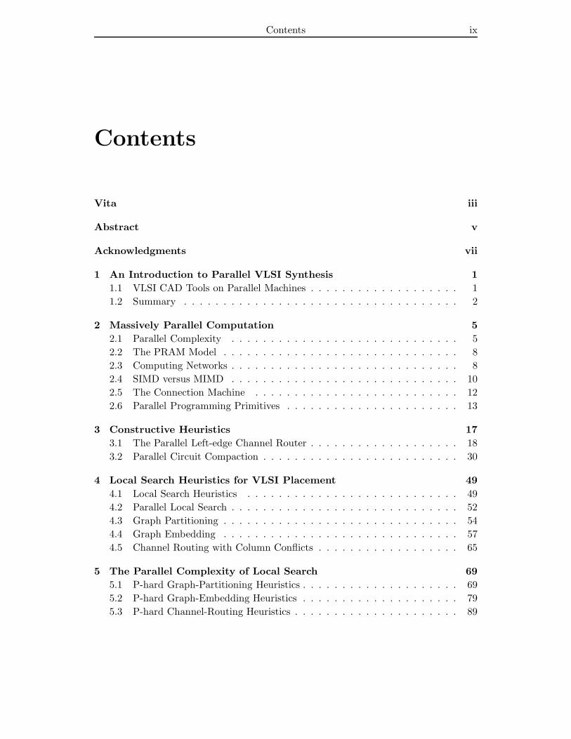
Contents
Vita iii
Abstract v
Acknowledgments vii
1 An Introduction to Parallel VLSI Synthesis 1
1.1 VLSI CAD Tools on Parallel Machines . . . . . . . . . . . . . . . . . . . 1
1.2 Summary . . . . . . . . . . . . . . . . . . . . . . . . . . . . . . . . . . . 2
2 Massively Parallel Computation 5
2.1 Parallel Complexity . . . . . . . . . . . . . . . . . . . . . . . . . . . . . 5
2.2 The PRAM Model . . . . . . . . . . . . . . . . . . . . . . . . . . . . . . 8
2.3 Computing Networks . . . . . . . . . . . . . . . . . . . . . . . . . . . . . 8
2.4 SIMD versus MIMD . . . . . . . . . . . . . . . . . . . . . . . . . . . . . 10
2.5 The Connection Machine . . . . . . . . . . . . . . . . . . . . . . . . . . 12
2.6 Parallel Programming Primitives . . . . . . . . . . . . . . . . . . . . . . 13
3 Constructive Heuristics 17
3.1 The Parallel Left-edge Channel Router . . . . . . . . . . . . . . . . . . . 18
3.2 Parallel Circuit Compaction . . . . . . . . . . . . . . . . . . . . . . . . . 30
4 Local Search Heuristics for VLSI Placement 49
4.1 Local Search Heuristics . . . . . . . . . . . . . . . . . . . . . . . . . . . 49
4.2 Parallel Local Search . . . . . . . . . . . . . . . . . . . . . . . . . . . . . 52
4.3 Graph Partitioning . . . . . . . . . . . . . . . . . . . . . . . . . . . . . . 54
4.4 Graph Embedding . . . . . . . . . . . . . . . . . . . . . . . . . . . . . . 57
4.5 Channel Routing with Column Conflicts . . . . . . . . . . . . . . . . . . 65
5 The Parallel Complexity of Local Search 69
5.1 P-hard Graph-Partitioning Heuristics . . . . . . . . . . . . . . . . . . . . 69
5.2 P-hard Graph-Embedding Heuristics . . . . . . . . . . . . . . . . . . . . 79
5.3 P-hard Channel-Routing Heuristics . . . . . . . . . . . . . . . . . . . . . 89
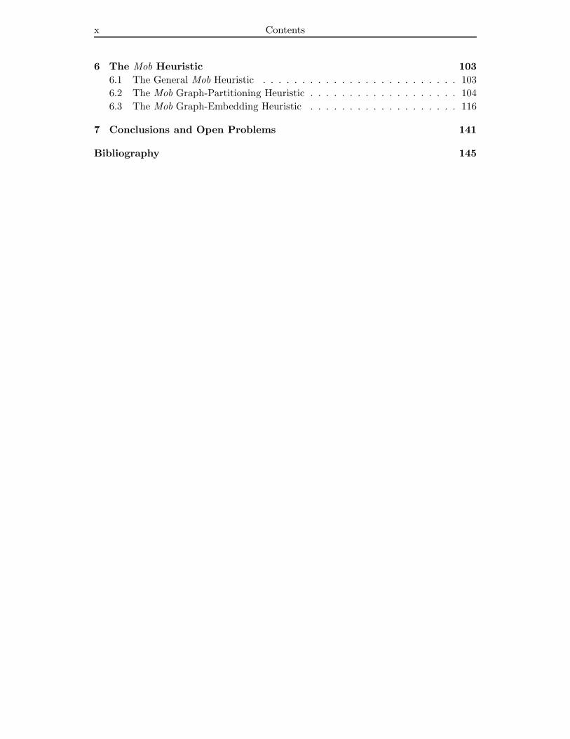
x Contents
6 The Mob Heuristic 103
6.1 The General Mob Heuristic . . . . . . . . . . . . . . . . . . . . . . . . . 103
6.2 The Mob Graph-Partitioning Heuristic . . . . . . . . . . . . . . . . . . . 104
6.3 The Mob Graph-Embedding Heuristic . . . . . . . . . . . . . . . . . . . 116
7 Conclusions and Open Problems 141
Bibliography 145
List of Tables xi
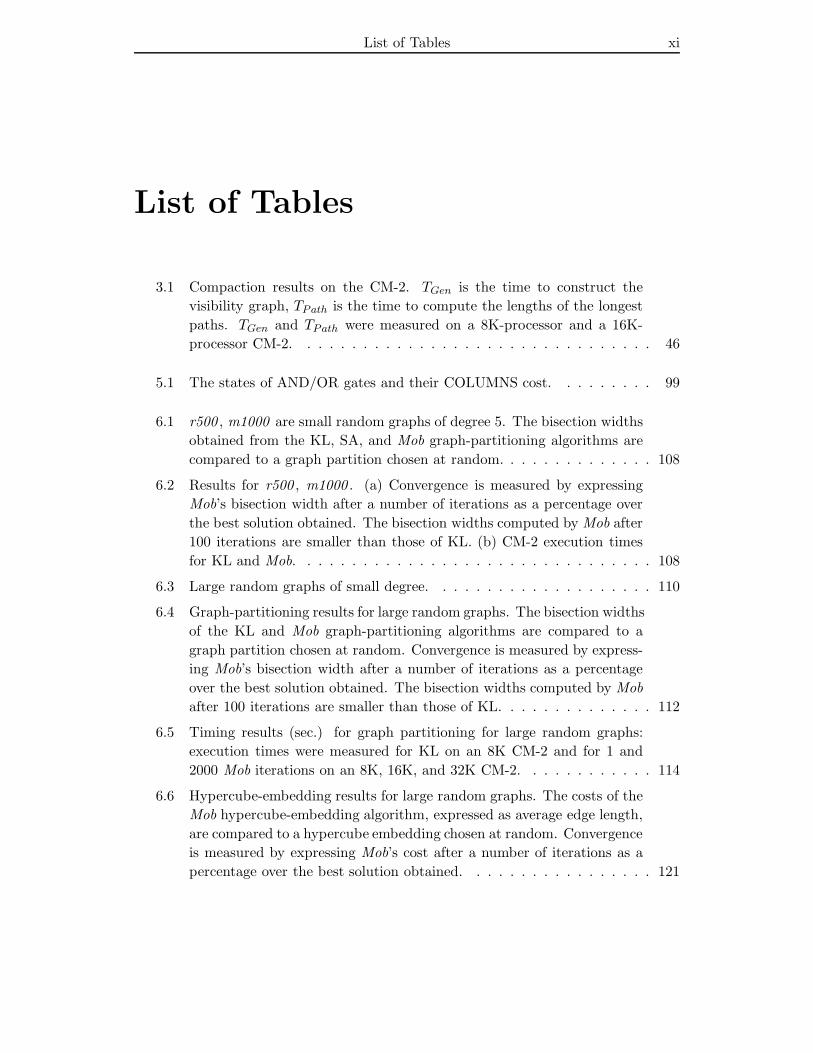
List of Tables
3.1 Compaction results on the CM-2. TGen is the time to construct the
visibility graph, TPath is the time to compute the lengths of the longest
paths. TGen and TPath were measured on a 8K-processor and a 16K-
processor CM-2. . . . . . . . . . . . . . . . . . . . . . . . . . . . . . . . 46
5.1 The states of AND/OR gates and their COLUMNS cost. . . . . . . . . 99
6.1 r500 , m1000 are small random graphs of degree 5. The bisection widths
obtained from the KL, SA, and Mob graph-partitioning algorithms are
compared to a graph partition chosen at random. . . . . . . . . . . . . . 108
6.2 Results for r500 , m1000 . (a) Convergence is measured by expressing
Mob’s bisection width after a number of iterations as a percentage over
the best solution obtained. The bisection widths computed by Mob after
100 iterations are smaller than those of KL. (b) CM-2 execution times
for KL and Mob. . . . . . . . . . . . . . . . . . . . . . . . . . . . . . . . 108
6.3 Large random graphs of small degree. . . . . . . . . . . . . . . . . . . . 110
6.4 Graph-partitioning results for large random graphs. The bisection widths
of the KL and Mob graph-partitioning algorithms are compared to a
graph partition chosen at random. Convergence is measured by express-
ing Mob’s bisection width after a number of iterations as a percentage
over the best solution obtained. The bisection widths computed by Mob
after 100 iterations are smaller than those of KL. . . . . . . . . . . . . . 112
6.5 Timing results (sec.) for graph partitioning for large random graphs:
execution times were measured for KL on an 8K CM-2 and for 1 and
2000 Mob iterations on an 8K, 16K, and 32K CM-2. . . . . . . . . . . . 114
6.6 Hypercube-embedding results for large random graphs. The costs of the
Mob hypercube-embedding algorithm, expressed as average edge length,
are compared to a hypercube embedding chosen at random. Convergence
is measured by expressing Mob’s cost after a number of iterations as a
percentage over the best solution obtained. . . . . . . . . . . . . . . . . 121
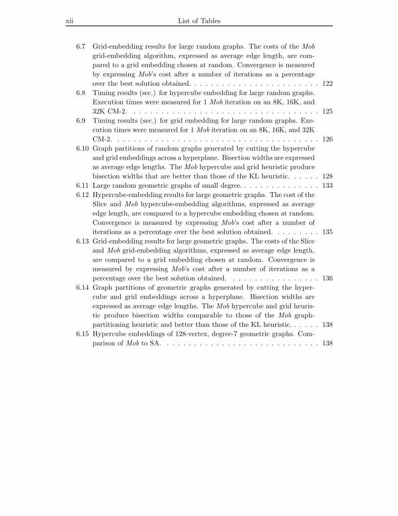
xii List of Tables
6.7 Grid-embedding results for large random graphs. The costs of the Mob
grid-embedding algorithm, expressed as average edge length, are com-
pared to a grid embedding chosen at random. Convergence is measured
by expressing Mob’s cost after a number of iterations as a percentage
over the best solution obtained. . . . . . . . . . . . . . . . . . . . . . . . 122
6.8 Timing results (sec.) for hypercube embedding for large random graphs.
Execution times were measured for 1 Mob iteration on an 8K, 16K, and
32K CM-2. . . . . . . . . . . . . . . . . . . . . . . . . . . . . . . . . . . 125
6.9 Timing results (sec.) for grid embedding for large random graphs. Exe-
cution times were measured for 1 Mob iteration on an 8K, 16K, and 32K
CM-2. . . . . . . . . . . . . . . . . . . . . . . . . . . . . . . . . . . . . . 126
6.10 Graph partitions of random graphs generated by cutting the hypercube
and grid embeddings across a hyperplane. Bisection widths are expressed
as average edge lengths. The Mob hypercube and grid heuristic produce
bisection widths that are better than those of the KL heuristic. . . . . . 128
6.11 Large random geometric graphs of small degree. . . . . . . . . . . . . . . 133
6.12 Hypercube-embedding results for large geometric graphs. The cost of the
Slice and Mob hypercube-embedding algorithms, expressed as average
edge length, are compared to a hypercube embedding chosen at random.
Convergence is measured by expressing Mob’s cost after a number of
iterations as a percentage over the best solution obtained. . . . . . . . . 135
6.13 Grid-embedding results for large geometric graphs. The costs of the Slice
and Mob grid-embedding algorithms, expressed as average edge length,
are compared to a grid embedding chosen at random. Convergence is
measured by expressing Mob’s cost after a number of iterations as a
percentage over the best solution obtained. . . . . . . . . . . . . . . . . 136
6.14 Graph partitions of geometric graphs generated by cutting the hyper-
cube and grid embeddings across a hyperplane. Bisection widths are
expressed as average edge lengths. The Mob hypercube and grid heuris-
tic produce bisection widths comparable to those of the Mob graph-
partitioning heuristic and better than those of the KL heuristic. . . . . . 138
6.15 Hypercube embeddings of 128-vertex, degree-7 geometric graphs. Com-
parison of Mob to SA. . . . . . . . . . . . . . . . . . . . . . . . . . . . . 138
List of Figures xiii
List of Figures
3.1 The connection graph G represents terminals to be connected by wires. 19
3.2 A channel routing of the connection graph G with minimum channel
width. . . . . . . . . . . . . . . . . . . . . . . . . . . . . . . . . . . . . . 20
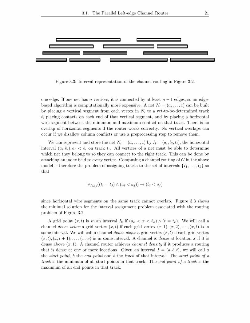
3.3 Interval representation of the channel routing in Figure 3.2. . . . . . . . 21
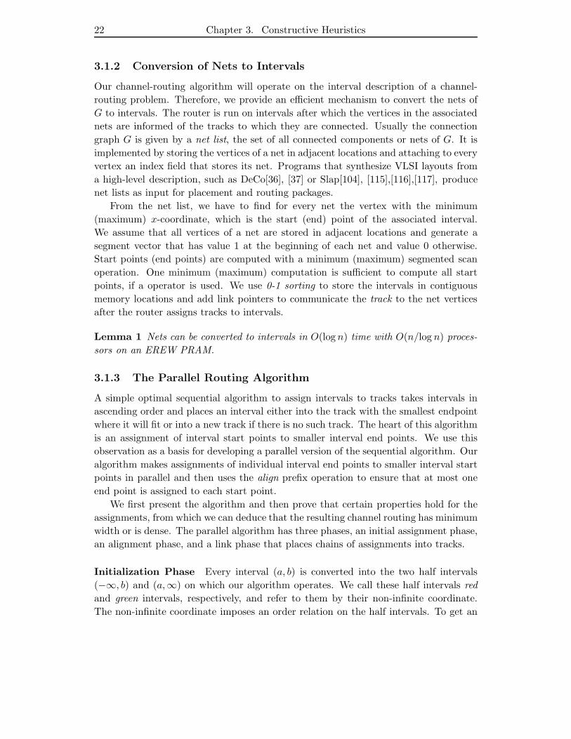
3.4 Assignments to Xi after initialization. . . . . . . . . . . . . . . . . . . . 23
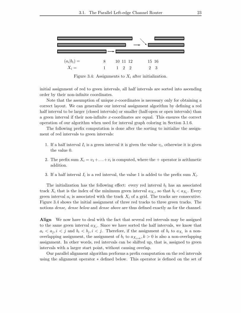
3.5 Assignments to Si after align prefix operation. . . . . . . . . . . . . . . . 24
3.6 A mismatch in an assignment of half intervals: b3 should have been
assigned to a2. . . . . . . . . . . . . . . . . . . . . . . . . . . . . . . . . 25
3.7 (a) Incorrect inefficient routing. (b) The nets are shortened. (c) The
column conflicts are removed. . . . . . . . . . . . . . . . . . . . . . . . . 29
3.8 (a) Uncompacted layout; minimum-distance constraints prevent rectan-
gle overlap. (b) Compacted layout. . . . . . . . . . . . . . . . . . . . . . 30
3.9 (a) Tiling of the layout: every constraint is replaced by a tile. (b) Tran-
sitive reduction of the constraint graph. . . . . . . . . . . . . . . . . . . 32
3.10 Building the visibility graph. Edges are placed along the trench whenever
a new rectangle appears in either the red shadow to the left of the trench
or the green shadow to the right of the trench. . . . . . . . . . . . . . . 35
3.11 (a) Two red shadows. (b) The red shadow data structures are updated
by inserting new event points. . . . . . . . . . . . . . . . . . . . . . . . . 36
3.12 The combined red shadow. . . . . . . . . . . . . . . . . . . . . . . . . . . 37
3.13 Reducing edges in the visibility graph by pattern matching. Only the
edge with the pattern (DOWN, UP) remains in the reduction; all others
are removed. . . . . . . . . . . . . . . . . . . . . . . . . . . . . . . . . . 39
3.14 Mergesort in reverse: (a) Four rectangles 00, 01, 10, 11, indexed by their
x-coordinate. (b) The rectangles are sorted by their y-coordinate, equiv-
alent to the final iteration of a mergesort on the y-coordinate. (c) The
rectangles after 0-1 sorting by the 2nd index bit. A left and a right
set are obtained, equivalent to the first iteration of a mergesort on the
y-coordinate. (d) The rectangles after 0-1 sorting the previous sets by
the 2nd index bit. The sets are again divided into left and right sets,
equivalent to the initial state before mergesort on the y-coordinate. . . 42
xiv List of Figures
3.15 Three uncompacted layouts with O(√
n) critical paths: (a) diamond
lattice, (b) irregular diamond lattice, (c) irregular mesh. . . . . . . . . . 45
3.16 Irregular diamond lattice. (a) Before compaction. (b) After compaction. 45
4.1 The simulated annealing (SA) heuristic. . . . . . . . . . . . . . . . . . . 50
4.2 Graph partitioning of a random graph. The two vertex sets of the par-
tition were placed on the upper and lower half-circle. (a) A randomly
generated solution. (b) A solution generated by the Mob heuristic. . . . 54
4.3 The Kernighan-Lin (KL) heuristic. . . . . . . . . . . . . . . . . . . . . . 56
4.4 16-to-1 grid embedding of a random graph: (a) A randomly generated
solution. (b) A solution generated by the Mob heuristic. . . . . . . . . . 58
4.5 1-to-1 grid embedding of a random graph: (a) A randomly generated
solution. (b) A solution generated by the Mob heuristic. . . . . . . . . 58
4.6 Transforming a channel-routing solution A into a solution B by subtrack
swaps. The set PB contains intervals in which the current track assign-
ment T (i) is equal to the desired track assignment TB(i) in solution B.
Track 2 contains the interval with the smallest end point RI2 and Ij is
the interval immediately to the right of RI2. Ik is the leftmost interval
in track TB(j). Since Ij is not in its target track (T (j) 6= TB(j)), the
subtracks containing Ij and Ik are swapped. No horizontal overlaps can
occur. . . . . . . . . . . . . . . . . . . . . . . . . . . . . . . . . . . . . . 67
5.1 Subgraphs equivalent to AND and OR gates. . . . . . . . . . . . . . . . 70
5.2 A monotone circuit and its equivalent subgraph. . . . . . . . . . . . . . 71
5.3 Schematic representation of G. . . . . . . . . . . . . . . . . . . . . . . . 72
5.4 Tree-like balancing subgraphs. . . . . . . . . . . . . . . . . . . . . . . . . 72
5.5 Operation of AND and OR gate subgraphs. . . . . . . . . . . . . . . . . 75
5.6 Reduction from graph partitioning to grid embedding: the graph G from
the proof of Theorem 9 in Section 5.1.2 is placed on the grid so that
positive-gain swaps on the grid correspond to positive-gain swaps in the
graph-partitioning problem. . . . . . . . . . . . . . . . . . . . . . . . . . 81
5.7 (a) Vertex vi in its initial position, before swap. (b) Regular positive-gain
swap of vi with a solitary vertex. . . . . . . . . . . . . . . . . . . . . . . 83
5.8 (a) Irregular swap, ∆y 6= 0. (b) Irregular swap, ∆y = 0,∆x > 1. . . . . 84
5.9 The overall construction of a channel-routing problem from circuit OM(C).
Circuit inputs, AND/OR gates, and connecting wires each have a pair
of center subtracks (horizontal segments). The anchor nets placed to the
left and right of the circuit subtracks prohibit swaps except between cen-
ter subtracks. The vertical segments of the circuit elements that cause
column conflicts are not shown. . . . . . . . . . . . . . . . . . . . . . . . 91
5.10 Circuit input Ia. (a) Ia = 0. (b) Ia = 1. . . . . . . . . . . . . . . . . . . 92
5.11 (a) OR gate Gr. (b) AND gate Gr. . . . . . . . . . . . . . . . . . . . . . 93
List of Figures xv
5.12 Connecting wire Wk. . . . . . . . . . . . . . . . . . . . . . . . . . . . . . 94
5.13 The state-transition graph of the circuit input Ia. (a) Ia = 0. (b) Ia = 1. 96
5.14 The state-transition graph of the wire Wk. . . . . . . . . . . . . . . . . . 98
5.15 The state-transition graph of the OR gate. . . . . . . . . . . . . . . . . . 100
6.1 The Mob heuristic . . . . . . . . . . . . . . . . . . . . . . . . . . . . . . 104
6.2 Ratios of best Mob bisection width to random bisection width for random
graphs plotted as a function of graph degree. . . . . . . . . . . . . . . . 113
6.3 Mob convergence behavior, measured by expressing Mob’s bisection width
after a number of iterations as a percentage over the best solution obtained.113
6.4 Ratios of best Mob embedding cost to random embedding cost for ran-
dom graphs plotted as a function of graph degree. . . . . . . . . . . . . 120
6.5 Mob convergence behavior, measured by expressing Mob’s bisection width
after a number of iterations as a percentage over the best solution obtained.124
6.6 (a) A random geometric graph on the unit plane. (b) Grid embedding
of the geometric graph. . . . . . . . . . . . . . . . . . . . . . . . . . . . 130
1
Chapter 1
An Introduction to Parallel VLSI
Synthesis
1.1 VLSI CAD Tools on Parallel Machines
We investigate the parallel complexity of VLSI (very large scale integration) CAD
(computer aided design) synthesis problems. Parallel algorithms are very appropriate
in VLSI CAD because computationally intensive optimization methods are needed to
derive “good” chip layouts. This thesis concentrates on problems related to parallel
layout synthesis. We believe that eventually the entire suite of CAD tools used to design
VLSI chips, from high-level specification to the generation of masks for fabrication, will
run on a massively parallel machine.
We find that for certain problems with polynomial-time serial complexity, it is
possible to find an efficient parallel algorithm that runs in polylogarithmic time. We
illustrate this by parallelizing the “left-edge” channel routing algorithm and the one-
dimensional constraint-graph compaction algorithm.
Curiously enough, we find P-hard, or inherently-difficult-to-parallelize algorithms
when certain key heuristics are used to get approximate solutions to NP-complete prob-
lems. In particular, we show that many local search heuristics for problems related to
VLSI placement are P-hard or P-complete. These include the Kernighan-Lin heuristic
and the simulated annealing heuristic for graph partitioning. We show that local search
heuristics for grid embeddings and hypercube embeddings based on vertex swaps are
P-hard, as are any local search heuristics that minimize the number of column conflicts
in a channel routing by accepting cost-improving swaps of tracks or subtracks. We
believe that the P-hardness reductions we provide in this thesis can be extended to
include many other important applications of local search heuristics.
We introduce the massively parallel Mob heuristic and report on experiments on the
CM-2 Connection Machine. The design of the Mob heuristic was influenced by the P-
hardness results. Mob can execute many moves of a local search heuristic in parallel. We

2 Chapter 1. An Introduction to Parallel VLSI Synthesis
applied our heuristic to the graph-partitioning, grid and hypercube-embedding prob-
lems, and report on an extensive series of experiments with our heuristic on the 32K-
processor CM-2 Connection Machine that show impressive reductions in edge costs.
We expect that parallel algorithms will supersede serial ones in all areas of VLSI
CAD, and believe that the Mob heuristic and P-hardness reductions given here can be
extended to include many other important applications of local search heuristics.
1.2 Summary
In Chapter 2 we give an introduction to parallel complexity classes, logspace reductions,
and to the boolean circuit-value problem, which is the canonical P-complete problem.
We introduce the PRAM model and discuss real-world implementation issues for paral-
lel machines. We discuss real-world implementation issues for parallel machines, where
the communication costs and area of interconnection networks must be taken into ac-
count. We also give a brief but impassioned discussion of the advantages of the SIMD
model over the MIMD model. We describe one successful massively parallel machine,
the CM-2 Connection Machine. The SIMD model constitutes a powerful and elegant
parallel programming methodology. Our parallel algorithms are designed to use local
operations plus simple parallel primitives such as sort, merge and parallel prefix.
In Chapter 3 we give constructive parallel heuristics for channel routing and com-
paction. In Section 3.1 we give an algorithm for two-layer channel routing of VLSI de-
signs. We have developed an optimal NC1(n) EREW PRAM algorithm that achieves
channel density[123]. This is a parallel version of the widely used “left-edge” algorithm
of Hashimoto and Stevens[58]. Our algorithm is also an optimal solution for the maxi-
mum clique and the minimum coloring problems for interval graphs and the maximum
independent set problem for co-interval graphs. Since the basic left-edge algorithm
does not deal with column conflicts, many variations and extensions of the left-edge
algorithm have been proposed, and our parallel algorithm can serve as a kernel to par-
allelize these extensions. Most of the more general two-layer channel routing problems
in which column conflicts and other quantities are to be minimized, are NP-complete,
so the more general two-layer channel routers are heuristics that produce routings of
very good quality but are not guaranteed to achieve minimum channel width or channel
density. Interestingly enough, we shall see in Section 5.3 that at least one such routing
heuristic is P-hard and thus unlikely to be parallelizable.
In Section 3.2 we give our results[124] for circuit compaction: a parallel algorithm
for computing the transitive reduction of an interval DAG. This is equivalent to a
parallel algorithm for computing a minimum-distance constraint DAG from a VLSI
layout. It is substantially simpler than a previously published serial algorithm. An
intermediate result during the execution of the above algorithm is a parallel algorithm
to construct a tiling or corner stitching, a geometrical data structure used in the Magic
VLSI layout system. All these computations take time O(log2 n) using O(n/log n)
1.2. Summary 3
processors on an EREW PRAM, so their processor-time product is optimal.
In Chapter 4 we introduce local search heuristics, of which KernighanLin, simulated
annealing, and steepest descent, are well-known examples. Such local search heuristics
have been established as the heuristics of choice for general graph-embedding problems.
The recent availability of general-purpose parallel processing hardware and the need to
solve very large problem instances have led to increasing interest in parallelizing local
search heuristics.
In Chapter 5 we show that certain local search heuristics in the area of parallel
placement algorithms and channel routing are P-complete or P-hard, or inherently
difficult to parallelize. Thus it is unlikely that a parallel algorithm exists that can
find even a local minimum solution in polylogarithmic time in the worst case. This
result puts into perspective experimental results reported in the literature: attempts
to construct the exact parallel equivalent of serial simulated-annealing-based heuristics
for graph embedding have yielded disappointing parallel speedups.
Section 5.1 deals with graph partitioning, the problem of partitioning the vertices
of a graph into two equal-sized sets so that the number of edges joining the sets is
minimum. We show that the Kernighan-Lin heuristic for graph partitioning is P-
complete and that the simulated annealing heuristic for graph partitioning is P-hard.
Section 5.2 deals with graph embedding on the grid and hypercube. Graph embed-
ding is the NP-complete problem of mapping one graph into another while minimizing
a cost function on the embedded edges of the graph. It finds application in VLSI
placement and also in minimizing of data movement in parallel computers. We show
that local search heuristics for grid embeddings and hypercube embeddings are P-hard
when the neighbors in the solution space are generated by swapping the embeddings
of two vertices.
In Section 5.3 we address the parallel complexity of a parallel channel routing
algorithm using simulated annealing as proposed by Brouwer and Banerjee[19]. We
show that any local search heuristic that minimizes the number of column conflicts in
a channel routing by accepting cost-improving swaps of tracks or subtracks is P-hard.
In Chapter 6 we introduce the massively parallel Mob heuristic and report on ex-
periments on the CM-2 Connection Machine. The design of the Mob heuristic was
influenced by the P-hardness results. Mob can execute many moves of a local search
heuristic in parallel. Due to excessive run times, heuristics previously reported in the
literature have been able to construct graph partitions and grid and hypercube em-
beddings only for graphs that were 100 to 1000 times smaller than those used in our
experiments. On small graphs, where simulated annealing and other heuristics have
been extensively tested, our heuristic was able to find solutions of quality at least as
good as simulated annealing.
In Section 6.2 we describe the Mob heuristic for graph partitioning, which swaps
large sets (mobs) of vertices across planes of a grid or hypercube. We report on an ex-
tensive series of experiments with our heuristic on the 32K-processor CM-2 Connection
Machine that show impressive reductions in the number of edges crossing the graph

4 Chapter 1. An Introduction to Parallel VLSI Synthesis
partition and run in less than nine minutes on random graphs of two million edges.
In Section 6.3 we describe the Mob heuristic for grid and hypercube embedding,
which swaps large sets (mobs) of vertices across planes of a grid or hypercube. Ex-
periments with our heuristic on the 32K-processor CM-2 Connection Machine show
impressive reductions in edge costs and run in less than 30 minutes on random graphs
of one million edges.
In Chapter 7 we present our conclusions and give an overview of open problems
and future work.
5
Chapter 2
Massively Parallel Computation
Many problems in VLSI design admit parallel solution. However, discovering such
solutions is often a considerable intellectual challenge, one that cannot be met today
through the use of a parallelizing compiler or speedup measurements. It is often con-
venient to develop parallel algorithms for the PRAM model described below. The
advantages of working with the PRAM model are that algorithms for it often are sim-
pler and faster than serial algorithms and can also give fundamental insight into the
nature of parallelism that can be applied to map these algorithms onto more realistic
parallel architectures.
We give an introduction to parallel complexity classes, logspace reductions, and
the boolean circuit-value problem, which is the canonical P-complete problem. We
introduce the PRAM model and discuss real-world implementation issues for parallel
machines. Interconnection networks and their communication costs must be taken into
account. We also give a brief but impassioned discussion of the advantages of the
SIMD model over the MIMD model. The SIMD model constitutes a powerful and
elegant parallel programming methodology. Our parallel algorithms are be designed
to use local operations plus simple parallel primitives such as sort, merge and parallel
prefix.
2.1 Parallel Complexity
We begin by defining P-complete and P-hard problems, the randomized decision class
BPP, and the boolean circuit-value problem CVP, which is the canonical P-complete
problem.
2.1.1 Classes and Completeness
Definition 1 A decision problem is a subset of 0, 1∗. A decision problem A is in
P , the class of polynomial-time problems, if there is a a deterministic polynomial-time
Turing machine T such that, if x ∈ A, then T accepts x and if x 6∈ A then T rejects x.
6 Chapter 2. Massively Parallel Computation
Definition 2 A decision problem A is logspace-reducible to a problem B if there is a
function g : 0, 1∗ → 0, 1∗ computable in logarithmic space (logspace) by a deter-
ministic Turing machine such that x ∈ A if and only if g(x) ∈ B.
Definition 3 A decision problem is P-complete if it is in P and every problem in
P is logspace-reducible to it. A decision problem is P-hard if every problem in P is
logspace-reducible to it.
Definition 4 A decision problem is in NC if it is solvable by a uniform class of circuits
with polynomial size and polylogarithmic depth. A class of circuits is uniform if there
is a Turing machine that for each integer n generates the nth circuit in polynomial
time.
The class NC was introduced by Pippenger[97]. If a P-complete problem is in NC,
then P is contained in NC[75], a highly unlikely result. Problems in NC can be solved
on a parallel machine with polynomially many processors in polylogarithmic time.
Since logspace-reducibility is transitive, if a problem A is P-complete and we can find
a logspace reduction of it to another problem B in P, then B is also P-complete. The
definition of P-hardness does not require that the decision problem be in P. A P-hard
problem is at least as hard to solve as a P-complete problem.
A “randomized Turing machine” RT[51] is a machine with an input tape and a
read-once, one-way binary “guess tape.” If a transition for a given state and input-
tape symbol is probabilistic, RT reads a string of k binary symbols from the guess tape,
treats it as an approximation to a real number in the interval (0,1) and uses it to select
a transition. The probability that a string x of length n is accepted (rejected) by a
randomized Turing machine making f(n) transitions is the number of strings of length
f(n) on the guess tape that causes x to be accepted (rejected), divided by the total
number of strings of length f(n). PP and BPP are classes of languages defined below
recognized by polynomial-time RTs.
Definition 5 A decision problem A ∈ PP if there is a a randomized polynomial-time
Turing machine RT such that if x ∈ A then Pr(RT accepts x) > 1/2 and if x 6∈ A
then Pr(RT rejects x) > 1/2.
The class PP is not very useful for our purposes. It can be shown that NP ⊆ PP [51].
We are interested in a higher degree of confidence in the outcome of the RT, that
characterized by the class BPP of polynomial-time RTs with bounded error probability,
as defined below.
Definition 6 A decision problem A ∈ BPP if there is a a randomized polynomial-time
Turing machine RT and an ǫ > 0 such that if x ∈ A then Pr(RT accepts x) > (1/2+ǫ)
and if x 6∈ A then Pr(RT rejects x) > (1/2 + ǫ).
2.1. Parallel Complexity 7
It is known that P ⊆ BPP
NP⊆ PP [51]. Every language in BPP can be recognized by
a polynomial-time randomized Turing machine RT with probability arbitrarily close to
1 by repeating the computation and taking the majority of the outcomes as the result.
It can be seen that with this construction the error probability decreases exponentially
with the number of repetitions. It is unknown whether there are problems logspace-
complete for BPP.
2.1.2 Circuits
A Boolean circuit is described by a straight-line program over a set of Boolean opera-
tions[113]. One output generated by the circuit is identified as significant and is called
the “value” of the circuit. The free variables are called “inputs” and are assigned val-
ues. A circuit corresponds to a directed acyclic graph (DAG) with Boolean function
labels on internal vertices.
Definition 7 The circuit-value problem (CVP) is the problem of computing the value
of a Boolean circuit from a description of the circuit and values for its inputs.
Theorem 1 CVP is P-complete.
The proof of Theorem 1 is due to Ladner[75], and is similar to the proof of Cook’s
seminal theorem that SAT is NP-complete[32]. The method of proof is to take the
description of a TM that on an input of length n runs in polynomial time p(n), and
transform this description into a boolean circuit.
We say a circuit element k depends on a circuit element i when it is connected to
an output of circuit element i, or when it is connected to an output of circuit element
j that depends on circuit element i.
Definition 8 The ordered circuit-value problem (OMCVP) is the problem of comput-
ing the value of a Boolean circuit OM(C) from a description of the circuit and values
for its inputs. The circuit elements in OM(C) are indexed so that when circuit element
k depends on gate i, then k > i.
We note that the circuit generated in the proof of Theorem 1 is ordered. This gives us
the following corollary:
Corollary 1 The ordered circuit-value problem OMCVP is P-complete.
Restricted versions of CVP are also P-complete. A monotone circuit uses only
the operations AND and OR, and the monotone circuit-value problem (MCVP) is P-
complete[52]. The planar circuit-value problem is also P-complete [52], but the planar
monotone circuit-value problem is in NC[53]. The fan-in/fan-out 2 circuit-value prob-
lem is P-complete, since any circuit can be translated in logspace into a circuit in which
both fan-in and fan-out of internal vertices are at most 2.
8 Chapter 2. Massively Parallel Computation
The dual-rail circuit DR(C) of a monotone circuit C consists of two subcircuits, C
and C, containing only ANDs and ORs. The subcircuit C is obtained by replacing each
AND in C with an OR and vice versa, and complementing the inputs. A very convenient
feature of the dual-rail circuit DR(C) is that exactly half of the inputs and half of the
circuit elements in DR(C) have value 1. It follows from the above construction that
the dual-rail monotone circuit-value problem (DRMCVP) is P-complete.
Local search heuristics, such as simulated annealing (SA)[69] and Kernighan-Lin
(KL)[68], evaluate functions that map solutions to neighboring solutions. To convert
these functions to decision problems, it is sufficient to mark one node in the graph and
to accept partitions in which the marked node changes sets under the heuristic mapping.
When we speak of the P-completeness or P-hardness of a local search heuristic, we refer
to the decision-based versions of these problems.
2.2 The PRAM Model
The PRAM (parallel random-access machine) is a very general model of computation
based upon an idealized multiprocessor machine with shared memory. Processors alter-
nate between reading from shared or local memory, doing an internal computation and
writing to shared or local memory. The cost of accessing a memory location by each
processor is constant, and communication costs are therefore ignored in this model.
The PRAM model is further refined by dealing with concurrent reads and writes. An
EREW PRAM admits exclusive read and write operations to the shared memory. A
CREW PRAM admits concurrent reads but exclusive write operations. The ERCW
and CRCW PRAMs are defined analogously. Unless otherwise specified, parallel time
complexities refer to the EREW model. Classes of problems that can be solved quickly
in parallel on the PRAM with a small number of processors have been identified. The
most important such class is NC, which was defined in Section 2.1. For conciseness,
we sometimes use the notation NCk(p) for an algorithm that runs in time O(logk n)
with O(p) processors on a problem of size n.
For a more detailed introduction to the PRAM model and a survey of existing work
see Cook[33], Karp and Ramachandran[67], the MIT class notes by Leighton et al.[81,
82], Leighton[78] Reif[103], Shmoys and Tardos[129], and Suaya and Birtwistle[132].
2.3 Computing Networks
In this section we give a brief overview of results in the areas of PRAM simulations on
computing networks, message routing and VLSI space-time tradeoffs, and how these
results apply to massively parallel computation. For detailed surveys of results in these
areas, and for further references, see Leighton[78], Leighton et al.[81,82], Leiserson[83],
Savage[114,118] and Suaya and Birtwistle[132].
The PRAM model introduced in Section 2.2 has been established as a very useful
2.3. Computing Networks 9
abstract tool for the development and analysis of parallel algorithms. However, the
designer of a practical parallel machine faces certain limitations that are ignored in
the PRAM model. A realistic machine will have non-trivial communication costs, and
must be packed onto a two-dimensional chip, or at least into three-dimensional volume.
Universal Networks The PRAM model assumes implicitly that the shared memory
can be accessed in O(1) time, an assumption that ignores communication costs. A more
realistic model is that of the computing network, which consists of a set of processors
with local memory connected to k other processors by wires along which messages are
passed. A universal network is a network that can efficiently simulate any network.
The hypercube is a universal computing network. Valiant and Brebner[17] have
shown that an n-processor hypercube can simulate an n-processor CRCW PRAM with
only O(log n) overhead, by giving a randomized routing algorithm that runs in O(log n)
time and uses queues of average length O(log n). Ranade[101] has shown that the
butterfly network is also universal, by giving a randomized routing algorithm that runs
in O(log n) time and uses queues of average length O(1). Other universal networks
include the cube-connected-cycles graph, the shuffle-exchange graph, and the DeBruijn
graph.
Lower Bounds In current technology, parallel computers and most other electronic
hardware are built out of two-dimensional chips. Switches and wires are formed out of
a few conductive or semiconductive layers on top of a semiconductor substrate, which
is typically silicon. We can place bounds on the minimum area required to implement
a given network. The following theorem is due to Thompson [135]:
Theorem 2 The area A required for the layout of a graph with bisection width w is at
least Ω(w2).
Using a three-dimensional medium to build the network does not help much. Thomp-
son’s result was extended to the layout of graphs in three-dimensions by Rosenberg[106].
Corollary 2 The volume V for the layout of a graph with bisection width w is Ω(w3/2).
By applying these lower bounds, Vuillemin[138] has shown that the layout area
of transitive functions with n inputs is Ω(n2). Transitive functions include binary
multiplication, cyclic shift, and convolution, for which efficient NC algorithms exist
on the PRAM. Therefore, any universal network requires a minimum layout area of
Ω(n2). A parallel computer that uses a hypercube or any other universal network
will consist mainly of wires. For instance, the n-processor hypercube has a bisection
width w = n/2. The degree of each processor is k = log n, the layout area A = Θ(n2)
and the volume V = Θ(n3/2). The n log n-processor cube-connected-cycles network
has bisection width w = n/2; the degree of each processor is k = 3 and layout area
10 Chapter 2. Massively Parallel Computation
A = Ω(n2); the n log n-processor butterfly has a bisection width w = n. The degree of
each processor is k = 4 and the layout area A = Ω(n2).
It would seem from the previous discussion that it is impossible to implement a
universal network in the real world. We note, however, that the above bounds are
asymptotic. Since the general-purpose parallel computing power of a universal network
is highly desirable, there is a strong incentive to “cheat” the asymptotic bounds by
allocating to the communication links more and more resources, such as money, area
and faster technology. The nervous system is an example of a successful architecture
in which this tradeoff between asymptotic behavior and functionality is evident: as
Mahowald and Mead[88] point out, the ratio of synapses (processors) to axons (wire)
in neural systems is about 1 to 100.
Area-Universal Networks An area-universal network is a network that can effi-
ciently simulate any network of comparable area. Area-universal networks include the
n-processor fat-tree[84] and the mesh-of-trees graph[82]. Both graphs have layouts with
area A = Ω(n log2 n).
The Speed of Light We note the implicit assumption for universal and area-universal
networks that the time to send a message between two processors is O(1) and inde-
pendent of wire length. We can alter the communication model by making the time
to send a message proportional to the length of the path along which it is sent. Let
f be a function computed by a circuit in which every output depends on n inputs. f
can be computed in time t = Ω( 3√
n). For example, in this model computing a sum
across all processors to find out whether all processors are switched on is impossible
in polylogarithmic time. The communication-time restrictions favor applications with
strong locality, such as physical simulations on a grid. We predict that this will change
the methods used in designing and analyzing algorithms.
2.4 SIMD versus MIMD
Architectures of parallel machines are often categorized in the literature by distin-
guishing SIMD and MIMD architectures. The processors of a SIMD (single instruction
multiple data) parallel machine share the same instruction stream, which is usually
distributed via broadcast by a control unit. The broadcast mechanism is separate from
and much simpler than the communications network. By necessity instructions are ex-
ecuted in lockstep. All current SIMD architectures associate processors with their own
local memories, but a shared-memory SIMD machine, in which each processor has its
own index pointer into the shared memory, is conceivable although not very practical.
A SIMD processor has the capability to switch itself off in response to the outcome of
a logical instruction; in this way IF..THEN..ELSE program constructs can be imple-
mented. Note that this results in idle processors. The processors of a MIMD (multiple

2.4. SIMD versus MIMD 11
instruction multiple data) parallel machine are fully independent: each processor has
its own program memory and as a rule executes asynchronously.
Both shared-memory and network MIMD machines have been built. The shared-
memory machines, among which are the Encore Multimax, the Sequent, and the Cray
machines, tend to have few processors. MIMD machines with communication networks
include the BBN Butterfly, the Intel iPSC, and various implementations using the
Inmos Transputer processor.
At first sight the MIMD approach seems to be vastly more powerful. The two ar-
guments most often put forth in its favor are: (a) the ability to program each processor
independently gives the designer access to a richer and more clever set of algorithms.
(b) MIMD is more efficient; when a processor has finished its task, it can request a new
task to work on instead of sitting idle. However, both arguments in favor of MIMD are
illusory. The asynchronous nature of the MIMD machine makes it difficult to debug
and to measure execution times. We shall illustrate that in theory SIMD machines are
as powerful as MIMD machines.
It is straightforward to prove the following theorem:
Theorem 3 A MIMD program of time complexity T (n) can be simulated by a SIMD
program in time < cT (n), where c is a small constant.
Proof We use Mehlhorn‘s argument given in[89] to show that RAMs (random-access
machines) with separate read-only program storage are equivalent to RAMs in which
the program is stored in memory as data. We simulate the MIMD program on a
SIMD machine by storing the individual programs of each MIMD processor in the data
memory of each SIMD processor. The control unit issues the following instruction
stream:
Load instruction
Load operands
Execute instruction
Save operands
The program counter of each MIMD processors is now simply replaced by an index
register on the SIMD processor. Loading and saving data are simply implemented by
using index registers on the SIMD machine. If the SIMD processors are so simple that
no index registers are available, we can use the global communication mechanism of
the SIMD machine though this may add a polylogarithmic overhead to the simulation.
The instruction set of the MIMD processor is assumed to be constant and given
the current preference for RISC (reduced-instruction-set computer) architecture, quite
small: the SIMD machine simply loops through the whole instruction set; all processors
whose loaded instruction matches the broadcast instruction execute that instruction,
all other processors are turned off.
12 Chapter 2. Massively Parallel Computation
Note that all SIMD processors are still running the same program, but the program
simulates simple processors. 2
In practice, MIMD machines have so far failed to deliver performance equal to SIMD
machines such as the CM-2 or the MasPar machine. Furthermore, the discrepancy will
probably become larger in the future: it is very likely that in a few years general
purpose SIMD machines will be able to execute 1012 OPS (operations per second). As
mentioned in Section 2.3, the cost of communication will be dominant past the 1012
OPS threshold, and will bring a reevaluation of architecture model and algorithms.
2.5 The Connection Machine
The Connection Machine 2 (CM-2) is a massively parallel computer consisting of up
to 64K moderately slow one-bit processors[1,61]. It is organized as a 12-dimensional
hypercube with sixteen nodes at each corner of the hypercube. The CM-2 supports
virtual processors, which are simulated very efficiently in microcode. A user allocates
virtual processors that are then bound to physical processors for execution. The CM-2
usually obtains its peak performance when the ratio of virtual to real processors is
more than one. Additionally, 2K pipelined floating-point processors are available for
numerical computations.
Each one-bit processor has an associated memory of up to 1M bits, which is shared
by passing messages among processors. The CM-2 supports message combining on the
hardware level to avoid network congestion. In contrast to shared-memory machines,
concurrent writes are much faster than concurrent reads. The CM-2 also permits
communication along hypercube and multidimensional grid axes, which is substantially
faster than the general router.
The CM-2 is a SIMD machine: each processor executes the same instruction at the
same time unless it has been disabled. In practice, the SIMD approach simplifies de-
bugging, permits an elegant programming style, and does not limit the expressiveness
of algorithms. The processors have unique IDs and can switch themselves on or off
depending on the outcome of boolean tests. The CM-2 is programmed using parallel
variables (pvars) with the same name in each processor. System software supports em-
beddings of multidimensional pvars onto the hypercube. The CM-2 has local arithmetic
and boolean operations to act on pvars as well as operations to send and receive mes-
sages to grid neighbors or arbitrary locations. Some of these operations set condition
bits which determine whether or not a processor is involved in subsequent operations.
Higher-level primitives are provided on the Connection Machine, including sorting,
reduction operations that combine values from each active processor, such as a global
OR operation, and the powerful scan operations. Scans are prefix operations introduced
by Iverson as part of the APL programming language[64]. Blelloch[12,13] shows how
the scan operation can be used as a powerful atomic programming primitive. (See
Section 2.6.)

2.6. Parallel Programming Primitives 13
The CM-2 supports numerous scan and also segmented scan operations in which a
series of scans is performed on contiguous regions of a linear array. The scan operation
runs in time logarithmic in the number of virtual processors on the CM-2.
Our Mob heuristic was implemented in the C language with calls to Paris (Release
5.1), the high-level assembly language of the CM-2.
2.6 Parallel Programming Primitives
Most parallel algorithms can be specified in a procedural form by using as parallel
programming primitives a number of simple operations, such as vector arithmetic,
parallel prefix and sorting. These operations greatly facilitate the mapping of parallel
algorithms development for the PRAM model onto realistic machines, such as the
Encore, a bus-based shared-memory machine, the Alliant, a pipelined multiprocessor,
and the CM-2 Connection Machine, a SIMD machine with a hypercube network.
2.6.1 Parallel Prefix
A prefix or scan operation applies an associative operator ∗ to a linear array and
produces a second linear array. If the first array has xi as its ith element and the
second has Si as its ith element, then a scan of the array x produces the array S of
partial products with Si = x1 ∗ . . . ∗ xi. With addition as the associative operator, it
computes a running sum, whereas with the copy operation it spreads a value into an
array of locations.
Prefix operations can be computed in time O(log n) with O(n/log n) processors
on an EREW PRAM and the constants hidden in the asymptotic notation are very
small. Minimum, addition, multiplication and boolean operations such as AND, OR,
EXOR, and bitwise addition are all associative operations. Fast and efficient parallel
algorithms can be developed through the use of more complex associative operators.
Ladner and Fischer[76] gave a circuit of depth ⌈log n⌉ and size 4n to compute the
parallel prefix, and showed how prefix computations could be applied to derive elegant
solutions to problems like binary addition. Fich[46] and Snir[130] have given precise
upper and lower bounds for prefix circuits.
Segmented Scan Occasionally it is necessary to compute the prefix sums of several
groups of elements. If these groups are stored in adjacent memory locations, one prefix
computation suffices if the operator ∗ is replaced by the following modified operator +:
(a + b).x := if (a.group == b.group) then a.x * b.x
else b.x
(a + b).group := b.group
where each element a is replaced by a value field a.x and a group field a.group. Each
group must have a unique index. It is easy to show that if ∗ is associative then +

14 Chapter 2. Massively Parallel Computation
is associative. This modification is called segmented prefix or segmented scan in the
literature. In the CM-2 implementation of the segmented scan, a segment vector is
used instead of a group field to save memory space[12,13]; the segment vector is 1 for
the first element of a group, and 0 otherwise. The group field can be reconstructed by
simply computing the addition prefix of the segment vector.
Copy The COPY prefix, which spreads a value to adjacent elements, is used to
distribute information in an array. It is usually used in conjunction with segment
fields.
a COPY b := a
0-1 Sorting Given an n-element array, let m < n of the elements be marked. We
want to reorder the array so that the marked elements are at the head of the array. This
can be achieved by assigning a 1 to marked elements and a 0 to unmarked elements and
then computing prefix sums of the addition operator to find new consecutive locations
for the marked elements. A similar computation can be done to move the unmarked
elements to the end of the array. The bounds of 0-1 sorting are those of parallel prefix.
2.6.2 List Ranking
List ranking is a generalization of the prefix sum problem on linked lists. The same
asymptotic bounds hold, but the algorithm is more complicated than parallel prefix.
See Karp and Ramachandran[67] for a detailed description and further references.
2.6.3 Merging and Sorting
Valiant[137] has shown that two ordered sets of size m and n, m ≤ n, can be merged in
time O(log log n) on a m + n processor CREW PRAM. Borodin and Hopcroft[16] have
shown that the time bound is tight. Also, Shiloach and Vishkin[128] have shown that
two sets can be merged in time O(log n) on a O(n/log n) processor CREW PRAM, a
processor-time bound that is optimal. Bilardi and Nicolau[11] give a merge algorithm
with the same bounds on the EREW PRAM.
For sorting, the AKS-network by Ajtai, Komlos, and Szemeredi[3] achieved optimal
O(log n) asymptotic time complexity, and can be implemented on the PRAM with
O(n) processors, as shown by Leighton [80]. It should be noted that these theoretically
optimal sorting algorithms have unrealistically large coefficients.
Cole[31] gives an algorithm based on mergesort that works in optimal O(log n)
time on an O(n)-processor CREW PRAM, and can be modified to work on the EREW
model. Bilardi and Nicolau[11] have given an optimal EREW PRAM algorithm based
on bitonic mergesort that runs in O(log n) time and O(n) processors with smaller
constants than[31]. In practical applications, however, Batcher’s bitonic sorting algo-
rithm[7] running in O(log2 n) time on an n-processor EREW PRAM is still preferable.
2.6. Parallel Programming Primitives 15
2.6.4 Connected Components
Hirschberg et al.[62] have shown that the connected components of a n-vertex, m-edge
graph can be found in O(log2 n) time on an O(n + m) processor EREW PRAM. The
set of vertices forming a connected component is represented by a canonical element,
the vertex with the smallest index.

17
Chapter 3
Constructive Heuristics
One goal of VLSI synthesis is to derive “good” chip layouts. We assume here that it is
possible to formulate what constitutes a good chip layout. We can specify that a design
should optimize area, power consumption, clock speed, or any other parameter. Given a
precise definition of an optimization problem, finding optimal solutions to this problem
is in most cases NP-hard, and we must use heuristics to get approximate solutions.
The process of defining “perfection” by selecting which parameter or parameters to
optimize may involve trial and error and is in itself a heuristic.
We can distinguish between constructive and iterative heuristics, a classification
introduced by Preas and Karger[98] for placement problems but used here for any
type of heuristic. A constructive heuristic computes one solution to a problem without
trying to improve on that solution. Iterative heuristics which we also call local search
heuristics, take a solution to a problem obtained by a constructive heuristic and make
changes to this solution in the hope of improving upon it. A constructive heuristic
exploits structure and regularity present in a problem instance to construct approximate
solutions. Constructive heuristics work well in restricted cases and lend themselves to
the derivation of bounds on the running time and the quality of the approximate
solution.
In this chapter we demonstrate how some constructive heuristics can be efficiently
parallelized to run in NC. We give constructive parallel heuristics for channel routing
and compaction. In Section 3.1 we give an algorithm for two-layer channel routing
of VLSI designs. In Section 3.2 we present a parallel algorithm for computing the
transitive reduction of an interval DAG, which is used for circuit compaction. We give
a survey of constructive heuristics for graph embedding in Section 4.4.8.
Chapters 4, 5, and 6 deal with parallel iterative heuristics. We define local search
heuristics, introduce some placement-related problems to which local search has been
applied, and give an overview of the vast volume of previous work in the field. We
show that certain local search heuristics are hard to parallelize and give experimental
results for our parallel Mob heuristic.
18 Chapter 3. Constructive Heuristics
3.1 The Parallel Left-edge Channel Router
The channel-routing problem P in VLSI design consists of terminals located above and
below a rectangular integer grid called a channel. Sets of terminals, called nets, are to
be connected electrically by wire segments that are placed on the integer grid.
In two-layer channel routing, a net is implemented by one horizontal segment in
one layer and vertical segments linking the horizontal segment to the terminals in the
other layer. Vias connect segments on different layers. A conflict occurs when vias or
segments belonging to different nets overlap in the same layer. A column conflict occurs
if two terminals on opposite sides of a channel have overlapping vertical segments. The
channel width is the number of tracks needed to route all nets. The maximum number
of nets intersecting any column is called channel density, with channel density ≤channel width. The goal of channel routing is to produce a routing without conflicts
while minimizing the number of tracks.
In this section we present an optimal O(log n) time, O(n) processor EREW PRAM
algorithm that achieves channel density[123]. The algorithm is a parallel version of the
“left-edge” algorithm developed by Hashimoto and Stevens[58] for PCB routing. The
parallel channel-routing algorithm was implemented on the CM-2 Connection Machine,
where it runs in time O(log2 n) with O(n) processors.
The basic left-edge algorithm does not deal with column conflicts, and thus many
variations and extensions have been proposed: Deutsch’s dogleg channel router[39],
Dolev et al.’s channel router[43], Fiduccia and Rivest’s greedy channel router[105],
Yoshimura and Kuh’s channel router[73], and YACR2 by Reed et al.[102]. The above
algorithms are all serial.
These heuristics for two-layer channel routing with column conflicts produce rout-
ings of very good quality but are not guaranteed to achieve minimum channel width
or channel density. Most of the more general two-layer channel routing problems are
NP-complete, as shown by LaPaugh[74], Szymanski[133], and Sarrafzadeh[110].
Brouwer and Banerjee[19] have applied parallel simulated annealing to the channel-
routing problem and have demonstrated that this approach yields routings of high
quality. We describe their approach in Section 4.5. In Section 5.3 we address the
question of how much speedup can be expected from a such a heuristic in the worst
case. We show that any local search heuristic that minimizes the number of column
conflicts in a channel routing by accepting cost-improving swaps of tracks or subtracks
is P-hard. Thus it is unlikely that a parallel algorithm exists that can find even a local
minimum solution in polylogarithmic time in the worst case, since that would imply
that every polynomial-time problem would have a similar solution.
In Section 3.1.1 we define two-layer routing in a rectilinear channel and we show how
to represent wires by horizontal intervals, which will be the input format of our parallel
algorithm. Section 3.1.2 deals with the conversion of the input connection graph into
an interval representation. All preprocessing is also in NC. In Section 3.1.3 we give the
routing algorithm, in Section 3.1.4 the proof of correctness and in Section 3.1.5 upper
3.1. The Parallel Left-edge Channel Router 19
w w w w w w w w w w w w w w w
w w w w w w w w w w w
\\
\\
\\
\\
\
bbbbbbbbbbbbbbb
ll
ll
ll
ll
ll
,,
,,
,,
,,
,,
bb
bbb
bb
bb
bbb
bb
,,
,,
,,
,,
,,
ZZ
ZZ
ZZ
ZZ
ZZ
ZZ
bbbbbbbbbbbbbbb
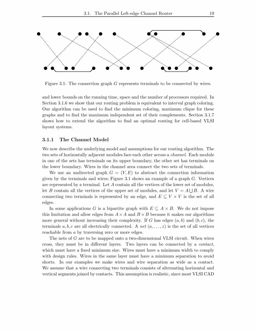
Figure 3.1: The connection graph G represents terminals to be connected by wires.
and lower bounds on the running time, space and the number of processors required. In
Section 3.1.6 we show that our routing problem is equivalent to interval graph coloring.
Our algorithm can be used to find the minimum coloring, maximum clique for these
graphs and to find the maximum independent set of their complements. Section 3.1.7
shows how to extend the algorithm to find an optimal routing for cell-based VLSI
layout systems.
3.1.1 The Channel Model
We now describe the underlying model and assumptions for our routing algorithm. The
two sets of horizontally adjacent modules face each other across a channel. Each module
in one of the sets has terminals on its upper boundary, the other set has terminals on
the lower boundary. Wires in the channel area connect the two sets of terminals.
We use an undirected graph G = (V,E) to abstract the connection information
given by the terminals and wires; Figure 3.1 shows an example of a graph G. Vertices
are represented by a terminal. Let A contain all the vertices of the lower set of modules,
let B contain all the vertices of the upper set of modules, and let V = A⋃
B. A wire
connecting two terminals is represented by an edge, and E ⊆ V × V is the set of all
edges.
In some applications G is a bipartite graph with E ⊆ A × B. We do not impose
this limitation and allow edges from A×A and B×B because it makes our algorithms
more general without increasing their complexity. If G has edges (a, b) and (b, c), the
terminals a, b, c are all electrically connected. A net (a, . . . , z) is the set of all vertices
reachable from a by traversing zero or more edges.
The nets of G are to be mapped onto a two-dimensional VLSI circuit. When wires
cross, they must be in different layers. Two layers can be connected by a contact,
which must have a fixed minimum size. Wires must have a minimum width to comply
with design rules. Wires in the same layer must have a minimum separation to avoid
shorts. In our examples we make wires and wire separation as wide as a contact.
We assume that a wire connecting two terminals consists of alternating horizontal and
vertical segments joined by contacts. This assumption is realistic, since most VLSI CAD

20 Chapter 3. Constructive Heuristics
Figure 3.2: A channel routing of the connection graph G with minimum channel width.
tools, data interchange formats and mask-making facilities do not allow rectangles with
arbitrary orientations.
When wires run on top of each other for a long stretch, there is the possibility of
electrical interference, called crosstalk. To avoid crosstalk and to simplify the routing
problem further, horizontal segments are placed on one layer and vertical segments are
placed on another layer.
Channel routing is a mapping of G onto an integer grid. The mapping of the vertex
sets A and B onto the grid is determined in part by the fixed x-coordinates of the
terminals. The channel is the portion of the grid between the two sets of vertices. A
track is a horizontal grid line. We assume a rectangular channel, meaning that the
vertices in each set are collinear, both sets are parallel and the channel contains no
obstacles. Each vertex v can be represented by its x-coordinate on the grid and its
set membership. The y-coordinate of all v ∈ A is 0. The y-coordinate of all v ∈ B is
w+1, where the channel width w is defined as the number of tracks needed to route G.
The channel length can either be infinite, as required by Fiduccia and Rivest’s greedy
channel router [105], or can be bounded by the minimum and maximum x-coordinates
of the vertices. The goal of our routing algorithm is to minimize channel width. The
layout of G in Figure 3.2 has minimum channel width.
Once the x-coordinates of the vertices are fixed we can compute the channel density,
which is a lower bound on the channel width. Count the number of nets crossing each
vertical grid line. Independently of how these nets are mapped on the grid, they must
cross that column at least once and will take up at least one grid point on that vertical
column. We will prove that our parallel algorithm always achieves this lower bound
when we impose the restriction that all terminals must have unique x-coordinates.
(This is done to avoid column conflicts.)
Interval Representation A net Ni = (a, . . . , z) is a set of vertices that are in the
same connected component of G. Our routing algorithm operates on nets of G, not
edges. The reason is that the operation of routing a net on a grid is as simple as routing
3.1. The Parallel Left-edge Channel Router 21
Figure 3.3: Interval representation of the channel routing in Figure 3.2.
one edge. If one net has n vertices, it is connected by at least n − 1 edges, so an edge-
based algorithm is computationally more expensive. A net Ni = (a, . . . , z) can be built
by placing a vertical segment from each vertex in Ni to a yet-to-be-determined track
t, placing contacts on each end of that vertical segment, and by placing a horizontal
wire segment between the minimum and maximum contact on that track. There is no
overlap of horizontal segments if the router works correctly. No vertical overlaps can
occur if we disallow column conflicts or use a preprocessing step to remove them.
We can represent and store the net Ni = (a, . . . , z) by Ii = (ai, bi, ti), the horizontal
interval (ai, bi), ai < bi on track ti. All vertices of a net must be able to determine
which net they belong to so they can connect to the right track. This can be done by
attaching an index field to every vertex. Computing a channel routing of G in the above
model is therefore the problem of assigning tracks to the set of intervals I1, . . . , Ik so
that
∀Ii,Ij((ti = tj) ∧ (ai < aj)) → (bi < aj)
since horizontal wire segments on the same track cannot overlap. Figure 3.3 shows
the minimal solution for the interval assignment problem associated with the routing
problem of Figure 3.2.
A grid point (x, t) is in an interval Ik if (ak < x < bk) ∧ (t = tk). We will call a
channel dense below a grid vertex (x, t) if each grid vertex (x, 1), (x, 2), . . . , (x, t) is in
some interval. We will call a channel dense above a grid vertex (x, t) if each grid vertex
(x, t), (x, t + 1), . . . , (x,w) is in some interval. A channel is dense at location x if it is
dense above (x, 1). A channel router achieves channel density if it produces a routing
that is dense at one or more locations. Given an interval I = (a, b, t), we will call a
the start point, b the end point and t the track of that interval. The start point of a
track is the minimum of all start points in that track. The end point of a track is the
maximum of all end points in that track.
22 Chapter 3. Constructive Heuristics
3.1.2 Conversion of Nets to Intervals
Our channel-routing algorithm will operate on the interval description of a channel-
routing problem. Therefore, we provide an efficient mechanism to convert the nets of
G to intervals. The router is run on intervals after which the vertices in the associated
nets are informed of the tracks to which they are connected. Usually the connection
graph G is given by a net list, the set of all connected components or nets of G. It is
implemented by storing the vertices of a net in adjacent locations and attaching to every
vertex an index field that stores its net. Programs that synthesize VLSI layouts from
a high-level description, such as DeCo[36], [37] or Slap[104], [115],[116],[117], produce
net lists as input for placement and routing packages.
From the net list, we have to find for every net the vertex with the minimum
(maximum) x-coordinate, which is the start (end) point of the associated interval.
We assume that all vertices of a net are stored in adjacent locations and generate a
segment vector that has value 1 at the beginning of each net and value 0 otherwise.
Start points (end points) are computed with a minimum (maximum) segmented scan
operation. One minimum (maximum) computation is sufficient to compute all start
points, if a operator is used. We use 0-1 sorting to store the intervals in contiguous
memory locations and add link pointers to communicate the track to the net vertices
after the router assigns tracks to intervals.
Lemma 1 Nets can be converted to intervals in O(log n) time with O(n/log n) proces-
sors on an EREW PRAM.
3.1.3 The Parallel Routing Algorithm
A simple optimal sequential algorithm to assign intervals to tracks takes intervals in
ascending order and places an interval either into the track with the smallest endpoint
where it will fit or into a new track if there is no such track. The heart of this algorithm
is an assignment of interval start points to smaller interval end points. We use this
observation as a basis for developing a parallel version of the sequential algorithm. Our
algorithm makes assignments of individual interval end points to smaller interval start
points in parallel and then uses the align prefix operation to ensure that at most one
end point is assigned to each start point.
We first present the algorithm and then prove that certain properties hold for the
assignments, from which we can deduce that the resulting channel routing has minimum
width or is dense. The parallel algorithm has three phases, an initial assignment phase,
an alignment phase, and a link phase that places chains of assignments into tracks.
Initialization Phase Every interval (a, b) is converted into the two half intervals
(−∞, b) and (a,∞) on which our algorithm operates. We call these half intervals red
and green intervals, respectively, and refer to them by their non-infinite coordinate.
The non-infinite coordinate imposes an order relation on the half intervals. To get an
3.1. The Parallel Left-edge Channel Router 23
-
-@@R
(ai|bi) = 8 10 11 12 15 16
Xi = 1 1 2 2 2 3
Figure 3.4: Assignments to Xi after initialization.
initial assignment of red to green intervals, all half intervals are sorted into ascending
order by their non-infinite coordinates.
Note that the assumption of unique x-coordinates is necessary only for obtaining a
correct layout. We can generalize our interval assignment algorithm by defining a red
half interval to be larger (closed intervals) or smaller (half-open or open intervals) than
a green interval if their non-infinite x-coordinates are equal. This ensures the correct
operation of our algorithm when used for interval graph coloring in Section 3.1.6.
The following prefix computation is done after the sorting to initialize the assign-
ment of red intervals to green intervals:
1. If a half interval Ii is a green interval it is given the value vi, otherwise it is given
the value 0.
2. The prefix sum Xi = v1+ . . .+vi is computed, where the + operator is arithmetic
addition.
3. If a half interval Ii is a red interval, the value 1 is added to the prefix sum Xi.
The initialization has the following effect: every red interval bi has an associated
track Xi that is the index of the minimum green interval aXi, so that bi < aXi
. Every
green interval ai is associated with the track Xi of a grid. The tracks are consecutive.
Figure 3.4 shows the initial assignment of three red tracks to three green tracks. The
notions dense, dense below and dense above are thus defined exactly as for the channel.
Align We now have to deal with the fact that several red intervals may be assigned
to the same green interval aXi. Since we have sorted the half intervals, we know that
ai < aj , i < j and bi < bj, i < j. Therefore, if the assignment of bi to aXiis a non-
overlapping assignment, the assignment of bi to aXi+k, k > 0 is also a non-overlapping
assignment. In other words, red intervals can be shifted up, that is, assigned to green
intervals with a larger start point, without causing overlap.
Our parallel alignment algorithm performs a prefix computation on the red intervals
using the alignment operator ∗ defined below. This operator is defined on the set of
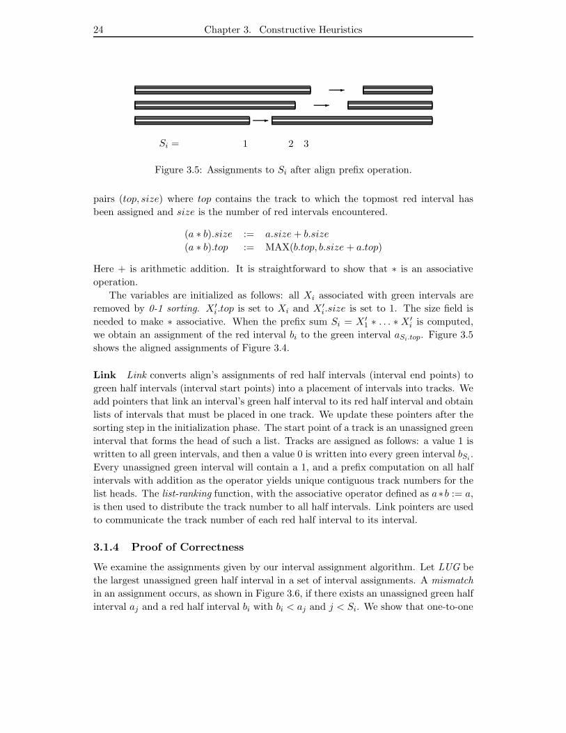
24 Chapter 3. Constructive Heuristics
-
-
-
Si = 1 2 3
Figure 3.5: Assignments to Si after align prefix operation.
pairs (top, size) where top contains the track to which the topmost red interval has
been assigned and size is the number of red intervals encountered.
(a ∗ b).size := a.size + b.size
(a ∗ b).top := MAX(b.top, b.size + a.top)
Here + is arithmetic addition. It is straightforward to show that ∗ is an associative
operation.
The variables are initialized as follows: all Xi associated with green intervals are
removed by 0-1 sorting. X ′i.top is set to Xi and X ′
i.size is set to 1. The size field is
needed to make ∗ associative. When the prefix sum Si = X ′1 ∗ . . . ∗ X ′
i is computed,
we obtain an assignment of the red interval bi to the green interval aSi.top. Figure 3.5
shows the aligned assignments of Figure 3.4.
Link Link converts align’s assignments of red half intervals (interval end points) to
green half intervals (interval start points) into a placement of intervals into tracks. We
add pointers that link an interval’s green half interval to its red half interval and obtain
lists of intervals that must be placed in one track. We update these pointers after the
sorting step in the initialization phase. The start point of a track is an unassigned green
interval that forms the head of such a list. Tracks are assigned as follows: a value 1 is
written to all green intervals, and then a value 0 is written into every green interval bSi.
Every unassigned green interval will contain a 1, and a prefix computation on all half
intervals with addition as the operator yields unique contiguous track numbers for the
list heads. The list-ranking function, with the associative operator defined as a∗b := a,
is then used to distribute the track number to all half intervals. Link pointers are used
to communicate the track number of each red half interval to its interval.
3.1.4 Proof of Correctness
We examine the assignments given by our interval assignment algorithm. Let LUG be
the largest unassigned green half interval in a set of interval assignments. A mismatch
in an assignment occurs, as shown in Figure 3.6, if there exists an unassigned green half
interval aj and a red half interval bi with bi < aj and j < Si. We show that one-to-one
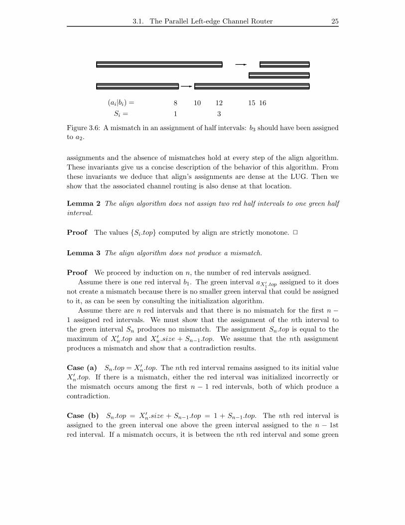
3.1. The Parallel Left-edge Channel Router 25
-
-
(ai|bi) = 8 10 12 15 16
Si = 1 3
Figure 3.6: A mismatch in an assignment of half intervals: b3 should have been assignedto a2.
assignments and the absence of mismatches hold at every step of the align algorithm.
These invariants give us a concise description of the behavior of this algorithm. From
these invariants we deduce that align’s assignments are dense at the LUG. Then we
show that the associated channel routing is also dense at that location.
Lemma 2 The align algorithm does not assign two red half intervals to one green half
interval.
Proof The values Si.top computed by align are strictly monotone. 2
Lemma 3 The align algorithm does not produce a mismatch.
Proof We proceed by induction on n, the number of red intervals assigned.
Assume there is one red interval b1. The green interval aX′
1.top assigned to it does
not create a mismatch because there is no smaller green interval that could be assigned
to it, as can be seen by consulting the initialization algorithm.
Assume there are n red intervals and that there is no mismatch for the first n −1 assigned red intervals. We must show that the assignment of the nth interval to
the green interval Sn produces no mismatch. The assignment Sn.top is equal to the
maximum of X ′n.top and X ′
n.size + Sn−1.top. We assume that the nth assignment
produces a mismatch and show that a contradiction results.
Case (a) Sn.top = X ′n.top. The nth red interval remains assigned to its initial value
X ′n.top. If there is a mismatch, either the red interval was initialized incorrectly or
the mismatch occurs among the first n − 1 red intervals, both of which produce a
contradiction.
Case (b) Sn.top = X ′n.size + Sn−1.top = 1 + Sn−1.top. The nth red interval is
assigned to the green interval one above the green interval assigned to the n − 1st
red interval. If a mismatch occurs, it is between the nth red interval and some green
26 Chapter 3. Constructive Heuristics
interval below the one assigned to the n − 1st interval. But then there is a mismatch
between the n − 1st red interval and this green interval. 2
Lemma 4 The align algorithm leaves a LUG after all red half intervals are assigned.
Proof Consider the green half interval (a1,∞). As a1 < ai, i ∈ 2, . . . , n and therefore
a1 < bi, i ∈ 1 . . . n, this green interval intersects with all red intervals. Thus there is at
least one unassigned green half interval. 2
Lemma 5 The assignments done by the align algorithm are dense at LUG.
Proof Assume the assignments are not dense at LUG. The green intervals are sorted
into ascending order. Therefore, the assignment is dense below the LUG. Thus, there
must be a hole above the LUG or a track with no interval that intersects the x-
coordinate of the LUG. A hole can be formed by the align algorithm in two ways:
Case (a) A hole is formed by an unassigned green interval. But that green inter-
val has a larger x-coordinate than the LUG, the largest unassigned green interval, a
contradiction.
Case (b) A hole is formed by a red interval with a smaller x-coordinate and (possibly)
a green interval with a x-coordinate larger than the LUG. But this implies that the
align algorithm has produced a mismatch, a contradiction. 2
Lemma 6 When the assignments are translated into a channel routing by the link
algorithm, the channel is dense at the LUG.
Proof Assume the channel is not dense at LUG. A hole in the channel routing can
occur in two ways:
Case (a) A hole occurs in a track that contains at least one interval to the right of
the hole and none to the left. The first such interval must have been an unassigned
green half interval produced by the align algorithm. But that green interval has a larger
x-coordinate than the LUG, a contradiction.
Case (b) A hole occurs in a track that contains at least one interval to left of the
hole. Before the link algorithm is applied there is a red half interval to the left of the
hole. This creates a hole above the LUG produced the align algorithm, which is a
contradiction. 2
3.1. The Parallel Left-edge Channel Router 27
3.1.5 Analysis of the Routing Algorithm
Let there be n intervals.
1. The cost of making the initial assignment to half intervals is the cost of sorting
2n integers plus a parallel prefix with addition as the associative operator. Time:
O(log n), Processors: O(n) on an EREW PRAM.
2. Align is a parallel prefix operation. Time: O(log n), Processors: O(n/log n) on
an EREW PRAM.
3. Link uses list ranking. Time: O(log n), Processors: O(n/log n) on an EREW
PRAM.
Our interval assignment algorithm is dominated by sorting during the initialization
phase.
Theorem 4 Channel routing of n nets can be done in time O(log n) with O(n) pro-
cessors on an EREW PRAM.
To achieve the bounds of this theorem we have assumed that the sorting algorithm
of[31] has been used. More practical algorithms add a factor of log n to the time.
Lower Bounds With our channel routing algorithm we can solve the interval overlap
problem, which is to determine whether n intervals on the line are disjoint. One track is
sufficient to route all nets if and only if there are no overlapping intervals. It has been
shown that every comparison-based algorithm for the interval overlap problem requires
Ω(n log n) comparisons (See Dobkin and Lipton[41], Ben-Or [8], and Preparata and
Shamos[100].) The processor-time product of our channel-routing algorithm is optimal.
3.1.6 Interval Graph Coloring
We now show how our routing algorithm can find the minimum coloring of an interval
graph. An undirected graph G is an interval graph if there exists a one-to-one mapping
from each vertex to an interval on the real line, and two intervals intersect if and only
if there is an edge between their two vertices. Interval graphs are a subset of perfect
graphs, which have the property that χ(G), the minimum coloring number of G, is equal
to ω(G), the size of the maximum clique of G. The complement graphs G = (V, E),
with (v,w) ∈ E ⇔ (v,w) 6∈ E, of interval graphs form a subset of comparability
graphs, which are also a subset of perfect graphs. A maximum clique in any graph
is a maximum independent set in the complement graph. Perfect graphs, interval
graphs, comparability graphs and their subsets have been studied extensively [54].
They are interesting because some of their properties can be computed efficiently while
the corresponding properties of general graphs are NP -hard. Mayr and Helmbold[60]
have found NC algorithms for maximum clique, minimum coloring in comparability
28 Chapter 3. Constructive Heuristics
graphs and maximum independent set and maximum matchings in interval and co-
comparability graphs.
A minimum coloring of an interval graph is an assignment of vertices to a minimum
number of colors such that two vertices of the same color have no edge between them.
This corresponds to an assignment of intervals to a minimum number of tracks such
that two intervals in the same track do not intersect. Our channel-routing algorithm is
therefore a minimum-coloring algorithm. Note that an actual coloring is constructed
here instead of just computing the coloring number χ(G).
Corollary 3 The minimum coloring and maximum clique of an n-node interval graph
and the maximum independent set of a co-interval graph can be computed from the
interval representation in time O(log n) with O(n) processors on an EREW.
The interval representation of an interval graph can be constructed in time O(log3 n)
with O(n4) processors on a CREW, as shown by Mayr and Helmbold[60]. Klein[70]
has given efficient parallel algorithms for recognizing and finding a maximum clique,
maximum independent set and optimal coloring of chordal graphs, of which interval
graphs are a subset. His algorithm for finding an optimal coloring takes O(log2 n) time
using a O(n + m) processor CRCW , where m is the number of edges.
3.1.7 Routing Library Modules
We presented a channel-routing algorithm that is in NC but works only in restricted
cases. We now give an NC extension that circumvents these restrictions in cell-based
silicon compilers such as DeCo or Slap. This allows our channel router to produce
significantly better layouts while using less computational resources than a general
channel-routing algorithm. When a circuit is built from standard library cells, there
is usually some freedom in choosing the exact position of the terminals. Designers
in the industrial world trade off slightly larger cell sizes to minimize area wasted in
routing. For example, the terminals in the 3-micron CMOS cell library[59] are far
apart. A system that uses such cells can avoid column conflicts by moving terminals to
unique locations. We now describe a procedure that places terminals so that no column
conflicts occur. The procedure also minimizes the horizontal length of each net, which
results in shorter intervals and therefore decreases channel density.
Lemma 7 Resolving column conflicts and minimizing channel density by allowing ter-
minals to occupy one of several adjacent locations can be done in O(log n) time on a
O(n)-processor EREW PRAM.
Proof Let us assume that a module can have any number of terminals, that the
position of each module is fixed and that modules cannot overlap. Each terminal
can be placed in at least two adjacent positions (x, x + 1). We assume that a net
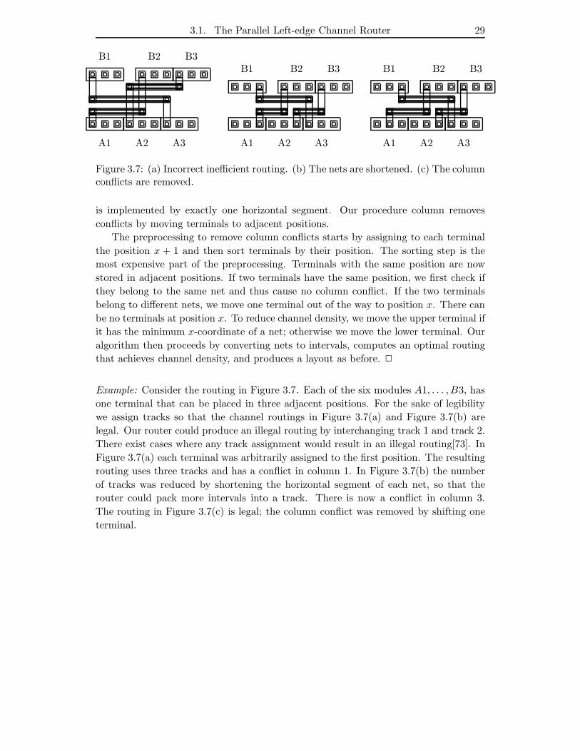
3.1. The Parallel Left-edge Channel Router 29
A1 A2 A3
B1 B2 B3
A1 A2 A3
B1 B2 B3
A1 A2 A3
B1 B2 B3
Figure 3.7: (a) Incorrect inefficient routing. (b) The nets are shortened. (c) The columnconflicts are removed.
is implemented by exactly one horizontal segment. Our procedure column removes
conflicts by moving terminals to adjacent positions.
The preprocessing to remove column conflicts starts by assigning to each terminal
the position x + 1 and then sort terminals by their position. The sorting step is the
most expensive part of the preprocessing. Terminals with the same position are now
stored in adjacent positions. If two terminals have the same position, we first check if
they belong to the same net and thus cause no column conflict. If the two terminals
belong to different nets, we move one terminal out of the way to position x. There can
be no terminals at position x. To reduce channel density, we move the upper terminal if
it has the minimum x-coordinate of a net; otherwise we move the lower terminal. Our
algorithm then proceeds by converting nets to intervals, computes an optimal routing
that achieves channel density, and produces a layout as before. 2
Example: Consider the routing in Figure 3.7. Each of the six modules A1, . . . , B3, has
one terminal that can be placed in three adjacent positions. For the sake of legibility
we assign tracks so that the channel routings in Figure 3.7(a) and Figure 3.7(b) are
legal. Our router could produce an illegal routing by interchanging track 1 and track 2.
There exist cases where any track assignment would result in an illegal routing[73]. In
Figure 3.7(a) each terminal was arbitrarily assigned to the first position. The resulting
routing uses three tracks and has a conflict in column 1. In Figure 3.7(b) the number
of tracks was reduced by shortening the horizontal segment of each net, so that the
router could pack more intervals into a track. There is now a conflict in column 3.
The routing in Figure 3.7(c) is legal; the column conflict was removed by shifting one
terminal.
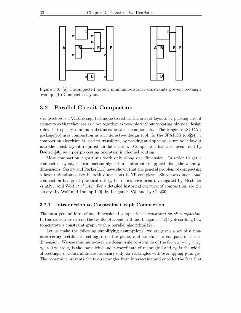
30 Chapter 3. Constructive Heuristics
A B
C
D
E F A B
C
D
E F
Figure 3.8: (a) Uncompacted layout; minimum-distance constraints prevent rectangleoverlap. (b) Compacted layout.
3.2 Parallel Circuit Compaction
Compaction is a VLSI design technique to reduce the area of layouts by packing circuit
elements so that they are as close together as possible without violating physical design
rules that specify minimum distances between components. The Magic VLSI CAD
package[96] uses compaction as an interactive design tool. In the SPARCS tool[24], a
compaction algorithm is used to transform, by packing and spacing, a symbolic layout
into the mask layout required for fabrication. Compaction has also been used by
Deutsch[40] as a postprocessing operation in channel routing.
Most compaction algorithms work only along one dimension. In order to get a
compacted layout, the compaction algorithm is alternately applied along the x and y-
dimensions. Sastry and Parker[111] have shown that the general problem of compacting
a layout simultaneously in both dimensions is NP-complete. Since two-dimensional
compaction has great practical utility, heuristics have been investigated by Mosteller
et al.[93] and Wolf et al.[141]. For a detailed historical overview of compaction, see the
surveys by Wolf and Dunlop[140], by Lengauer [85], and by Cho[30].
3.2.1 Introduction to Constraint Graph Compaction
The most general form of one-dimensional compaction is constraint-graph compaction.
In this section we extend the results of Doenhardt and Lengauer [42] by describing how
to generate a constraint graph with a parallel algorithm[124].
Let us make the following simplifying assumptions: we are given a set of n non-
intersecting rectilinear rectangles on the plane, and we want to compact in the x-
dimension. We use minimum-distance design-rule constraints of the form xi +aij ≤ xj ,
aij > 0 where xi is the lower left-hand x-coordinate of rectangle i and aij is the width
of rectangle i. Constraints are necessary only for rectangles with overlapping y-ranges.
The constraint prevents the two rectangles from intersecting and encodes the fact that
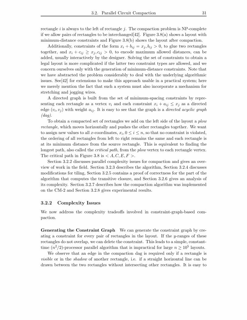
3.2. Parallel Circuit Compaction 31
rectangle i is always to the left of rectangle j. The compaction problem is NP-complete
if we allow pairs of rectangles to be interchanged[42]. Figure 3.8(a) shows a layout with
minimum-distance constraints and Figure 3.8(b) shows the layout after compaction.
Additionally, constraints of the form xi + bij = xj, bij > 0, to glue two rectangles
together, and xi + cij ≥ xj , cij > 0, to encode maximum allowed distances, can be
added, usually interactively by the designer. Solving the set of constraints to obtain a
legal layout is more complicated if the latter two constraint types are allowed, and we
concern ourselves only with the generation of minimum-distance constraints. Note that
we have abstracted the problem considerably to deal with the underlying algorithmic
issues. See[42] for extensions to make this approach usable in a practical system; here
we merely mention the fact that such a system must also incorporate a mechanism for
stretching and jogging wires.
A directed graph is built from the set of minimum-spacing constraints by repre-
senting each rectangle as a vertex vi and each constraint xi + aij ≤ xj as a directed
edge (vi, vj) with weight aij . It is easy to see that the graph is a directed acyclic graph
(dag).
To obtain a compacted set of rectangles we add on the left side of the layout a plow
rectangle, which moves horizontally and pushes the other rectangles together. We want
to assign new values to all x-coordinates, xi, 0 ≤ i ≤ n, so that no constraint is violated,
the ordering of all rectangles from left to right remains the same and each rectangle is
at its minimum distance from the source rectangle. This is equivalent to finding the
longest path, also called the critical path, from the plow vertex to each rectangle vertex.
The critical path in Figure 3.8 is < A,C,E, F >.
Section 3.2.2 discusses parallel complexity issues for compaction and gives an over-
view of work in the field. Section 3.2.3 describes the algorithm, Section 3.2.4 discusses
modifications for tiling, Section 3.2.5 contains a proof of correctness for the part of the
algorithm that computes the transitive closure, and Section 3.2.6 gives an analysis of
its complexity. Section 3.2.7 describes how the compaction algorithm was implemented
on the CM-2 and Section 3.2.8 gives experimental results.
3.2.2 Complexity Issues
We now address the complexity tradeoffs involved in constraint-graph-based com-
paction.
Generating the Constraint Graph We can generate the constraint graph by cre-
ating a constraint for every pair of rectangles in the layout. If the y-ranges of these
rectangles do not overlap, we can delete the constraint. This leads to a simple, constant-
time (n2/2)-processor parallel algorithm that is impractical for large n ≥ 105 layouts.
We observe that an edge in the compaction dag is required only if a rectangle is
visible or in the shadow of another rectangle, i.e. if a straight horizontal line can be
drawn between the two rectangles without intersecting other rectangles. It is easy to
32 Chapter 3. Constructive Heuristics
A B
C
D
E F A B
C
D
E F
Figure 3.9: (a) Tiling of the layout: every constraint is replaced by a tile. (b) Transitivereduction of the constraint graph.
see that the other constraints would never belong to any critical path. As we can now
“draw” the constraints onto the layout so that no two constraints cross, the associated
visibility graph is planar. The constraint graph in Figure 3.8(a) is planar.
It is possible to generate multiple copies of the same constraint. Note that a con-
straint can be replaced by a space tile that intersects no rectangle and no other space
tile. Figure 3.9(a) shows a tiling of the layout in Figure 3.8(a). A complete tiling of the
plane with n solid tiles can be completed with at most 3n+1 space tiles[96]. Therefore
the number of edges generated in a visibility graph is at most 3n − 3. (There are at
least four space tiles outside the layout.)
Doenhardt and Lengauer[42] observed that the number of edges in the graph can
be further reduced by computing the transitive reduction of the above graph: if two
vertices are connected by an edge and by a path of two or more edges, the edge can be
removed because any critical path includes the path and not the edge. A triangle-free
planar graph with at most 2n−4 edges is obtained in this way[56]. Figure 3.9(b) shows
the reduced constraint graph for the graph in Figure 3.8(a).
The algorithm computes what is also called the transitive reduction of an interval
dag. An undirected graph G is an interval graph if there exists a one-to-one mapping
from each vertex to an interval on the real line, and two intervals intersect if and only
if there is an edge between their two vertices. An interval dag is an interval graph in
which the edges are oriented so that no cycles are formed.
Relation to Other Work Doenhard and Lengauer[42] use a vertical plane-sweep
technique in conjunction with a leaf-linked tree data structure to obtain an O(n log n)-
time serial algorithm. Schlag et al.[127] investigate the serial complexity to compute
the visibility graph for rectilinear line segments. VLSI-specific assumptions such as
previously sorted coordinates and coordinates with a small range are addressed. It is
an open question whether the lower bound of O(n log n) time (or P ∗T ) still holds when

3.2. Parallel Circuit Compaction 33
the input is already sorted by both x- and y-coordinates. Lodi and Pagli[86] have given
a parallel algorithm for the mesh-of-trees network that computes all visibility pairs. The
algorithm runs in time O(log n) but always uses n2 processors, and thus is not efficient.
Atallah et al.[5] give a more general O(log n)-time, O(n)-processor CREW PRAM
algorithm to compute the trapezoidal decomposition of the plane, which is equivalent to
a tiling. A plane-sweep tree requiring O(n log n) space is shared between all processors.
It is unclear whether their techniques can be modified to work on a hypercube or mesh-
of-tree machine with small run-time constants. Edelsbrunner and Overmars[45] give a
serial algorithm to compute polygons visible to an outside observer, and introduce the
notion of “flatland graphics”, which are equivalent to our “skylines”.
We give a parallel algorithm to compute the reduction of an interval dag by first
generating the planar visibility graph and then removing unnecessary edges. It runs in
O(log2 n) time and has the same processor-time product as the serial algorithm with
one processor. Our parallel algorithm requires only linear arrays as data structures, so
we expect the constants hidden in the O() notation to be small for current hardware.
Solving the Constraint Graph The critical paths in the compaction constraint
graph can be computed with a single-source longest-path algorithm.
Serial Longest-Path As our graph is a dag and has O(n) edges, we can use a serial
O(n)-time algorithm based on a topological sorting of the edges[134]. In undirected
or cyclic graphs the longest-path problem can be reduced to the hamiltonian-cycles
problem and is thus NP-complete [49]. Code length and run-time constants of the serial
algorithm are extremely small. No DFS (depth-first-search) of the dag is required, and
the topological sorting can be obtained from the initial placement of the rectangles by
sorting the edges by their tail vertices.
Parallel Longest-Path A parallel algorithm is called efficient if its processor-time
product is within a polylog factor of optimal. Unfortunately, it is unknown whether
there exists an efficient parallel algorithm running in polylog time for the longest-
path problem for general, planar or even VLSI-specific graphs such as the transitive
reduction of an interval dag.
Savage[112] gives a simple all-sources shortest-path algorithm that is based on re-
peated boolean matrix multiplication. Unfortunately, it runs in O(log2 n) time on an
O(n3/log n) processor EREW PRAM. Apostolico et al.[4] have recently given an effi-
cient parallel shortest-path algorithm for a lattice dag. Both of these algorithms can
be modified for longest-path problems in dags. So far the fastest practical method is a
modification of the above serial algorithm, the implementation of which is described in
detail in Section 3.2.7. Both code and constants are very small, but the running time
is proportional to the maximum number of edges on any path in the dag, O(n) in the
worst case and O(√
n) for most VLSI layouts.
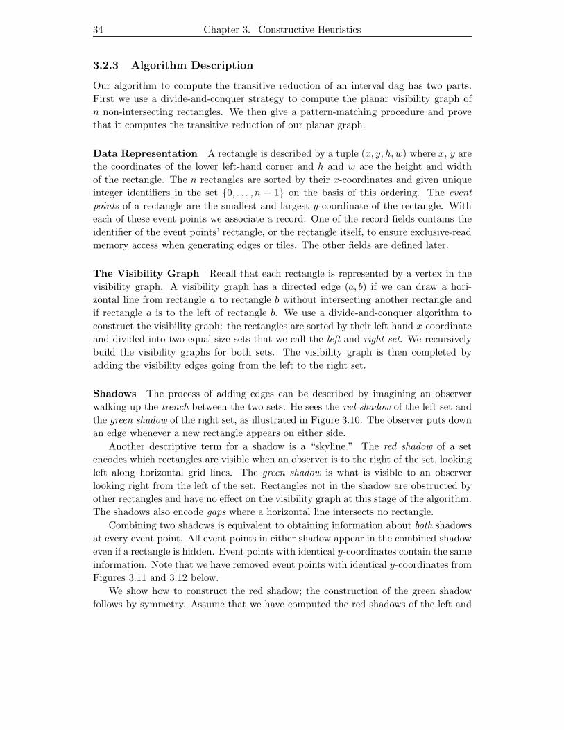
34 Chapter 3. Constructive Heuristics
3.2.3 Algorithm Description
Our algorithm to compute the transitive reduction of an interval dag has two parts.
First we use a divide-and-conquer strategy to compute the planar visibility graph of
n non-intersecting rectangles. We then give a pattern-matching procedure and prove
that it computes the transitive reduction of our planar graph.
Data Representation A rectangle is described by a tuple (x, y, h,w) where x, y are
the coordinates of the lower left-hand corner and h and w are the height and width
of the rectangle. The n rectangles are sorted by their x-coordinates and given unique
integer identifiers in the set 0, . . . , n − 1 on the basis of this ordering. The event
points of a rectangle are the smallest and largest y-coordinate of the rectangle. With
each of these event points we associate a record. One of the record fields contains the
identifier of the event points’ rectangle, or the rectangle itself, to ensure exclusive-read
memory access when generating edges or tiles. The other fields are defined later.
The Visibility Graph Recall that each rectangle is represented by a vertex in the
visibility graph. A visibility graph has a directed edge (a, b) if we can draw a hori-
zontal line from rectangle a to rectangle b without intersecting another rectangle and
if rectangle a is to the left of rectangle b. We use a divide-and-conquer algorithm to
construct the visibility graph: the rectangles are sorted by their left-hand x-coordinate
and divided into two equal-size sets that we call the left and right set. We recursively
build the visibility graphs for both sets. The visibility graph is then completed by
adding the visibility edges going from the left to the right set.
Shadows The process of adding edges can be described by imagining an observer
walking up the trench between the two sets. He sees the red shadow of the left set and
the green shadow of the right set, as illustrated in Figure 3.10. The observer puts down
an edge whenever a new rectangle appears on either side.
Another descriptive term for a shadow is a “skyline.” The red shadow of a set
encodes which rectangles are visible when an observer is to the right of the set, looking
left along horizontal grid lines. The green shadow is what is visible to an observer
looking right from the left of the set. Rectangles not in the shadow are obstructed by
other rectangles and have no effect on the visibility graph at this stage of the algorithm.
The shadows also encode gaps where a horizontal line intersects no rectangle.
Combining two shadows is equivalent to obtaining information about both shadows
at every event point. All event points in either shadow appear in the combined shadow
even if a rectangle is hidden. Event points with identical y-coordinates contain the same
information. Note that we have removed event points with identical y-coordinates from
Figures 3.11 and 3.12 below.
We show how to construct the red shadow; the construction of the green shadow
follows by symmetry. Assume that we have computed the red shadows of the left and
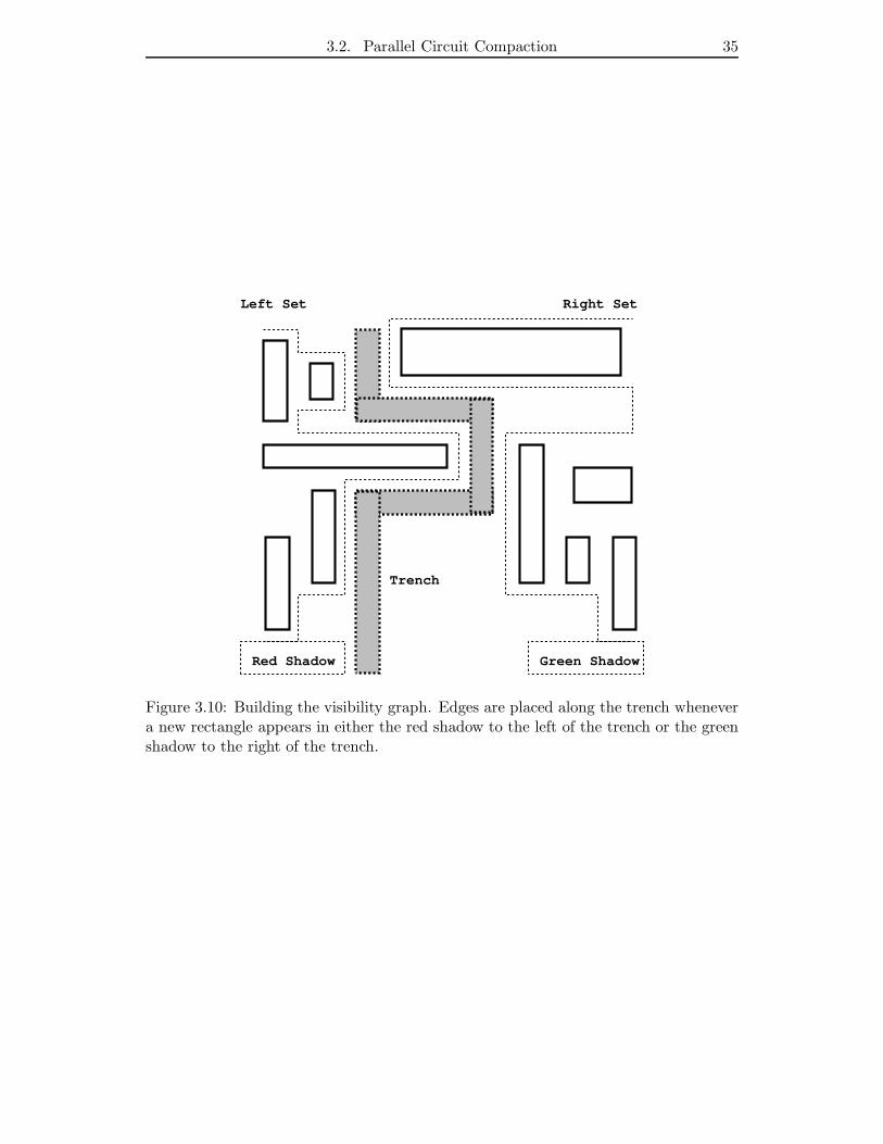
3.2. Parallel Circuit Compaction 35
Trench
Right SetLeft Set
Green ShadowRed Shadow
Figure 3.10: Building the visibility graph. Edges are placed along the trench whenevera new rectangle appears in either the red shadow to the left of the trench or the greenshadow to the right of the trench.
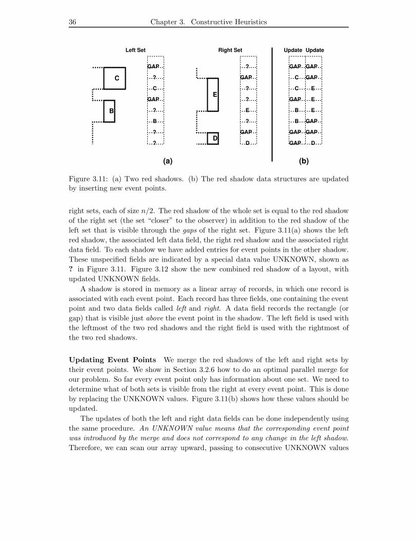
36 Chapter 3. Constructive Heuristics
B
C
E
D?
?
B
?
GAP
C
?
GAP
D
GAP
?
E
?
?
GAP
?
D
GAP
E
GAP
B
GAP
C
GAP
GAP
GAP
B
C
GAP
E
E
GAP
Left Set Right Set Update Update
(a) (b)
Figure 3.11: (a) Two red shadows. (b) The red shadow data structures are updatedby inserting new event points.
right sets, each of size n/2. The red shadow of the whole set is equal to the red shadow
of the right set (the set “closer” to the observer) in addition to the red shadow of the
left set that is visible through the gaps of the right set. Figure 3.11(a) shows the left
red shadow, the associated left data field, the right red shadow and the associated right
data field. To each shadow we have added entries for event points in the other shadow.
These unspecified fields are indicated by a special data value UNKNOWN, shown as
? in Figure 3.11. Figure 3.12 show the new combined red shadow of a layout, with
updated UNKNOWN fields.
A shadow is stored in memory as a linear array of records, in which one record is
associated with each event point. Each record has three fields, one containing the event
point and two data fields called left and right. A data field records the rectangle (or
gap) that is visible just above the event point in the shadow. The left field is used with
the leftmost of the two red shadows and the right field is used with the rightmost of
the two red shadows.
Updating Event Points We merge the red shadows of the left and right sets by
their event points. We show in Section 3.2.6 how to do an optimal parallel merge for
our problem. So far every event point only has information about one set. We need to
determine what of both sets is visible from the right at every event point. This is done
by replacing the UNKNOWN values. Figure 3.11(b) shows how these values should be
updated.
The updates of both the left and right data fields can be done independently using
the same procedure. An UNKNOWN value means that the corresponding event point
was introduced by the merge and does not correspond to any change in the left shadow.
Therefore, we can scan our array upward, passing to consecutive UNKNOWN values
3.2. Parallel Circuit Compaction 37
B
C
E
DD
GAP
E
B
GAP
GAP
C
E
E
GAP
Combined Shadow
C
E
E
E
B
D
Combined Set
Figure 3.12: The combined red shadow.
the last known value. The update can be done in parallel with the prefix computation
Si = x1 ∗ . . . ∗xi, where x1 is the bottom-most element in a shadow and ∗ is defined as:
c := a * b if (a == data and b == UNKNOWN) then c = a
else c = b
xi is the data value for the ith event point and Si is the updated data value that
replaces it. It is easy to see that ∗ is an associative operator. Sets of event points
that have identical y-coordinates are handled by a similar prefix operation that scans
downwards, instead of upwards, and works only on groups of event points with identical
y-coordinates. The first data fields may still contain the UNKNOWN value after the
update operation. For example, consider the lowest two event points in the left set in
Figure 3.11(a): these fields are changed to contain the gap value, because they always
represent a gap.
Computing Shadows Now that we know what is visible of both the left and right
red shadows at every event point, we can apply the local rule VISIBLE:
VISIBLE(gap, gap) := gap
VISIBLE(left_rectangle, gap) := left_rectangle
VISIBLE(gap, right_rectangle) := right_rectangle
VISIBLE(left_rectangle, right_rectangle) := right_rectangle
which says that in the combined red shadow a rectangle from the left set is visible
only if the right set contains a gap. Figure 3.12 shows the combined red shadow.
Computing Edges We have shown how to compute the shadows of a set of size n
from shadows of the same color of two sets of size n/2. To compute all edges in a set
of size n, we need the red shadow of the left set of size n/2 and the green shadow of
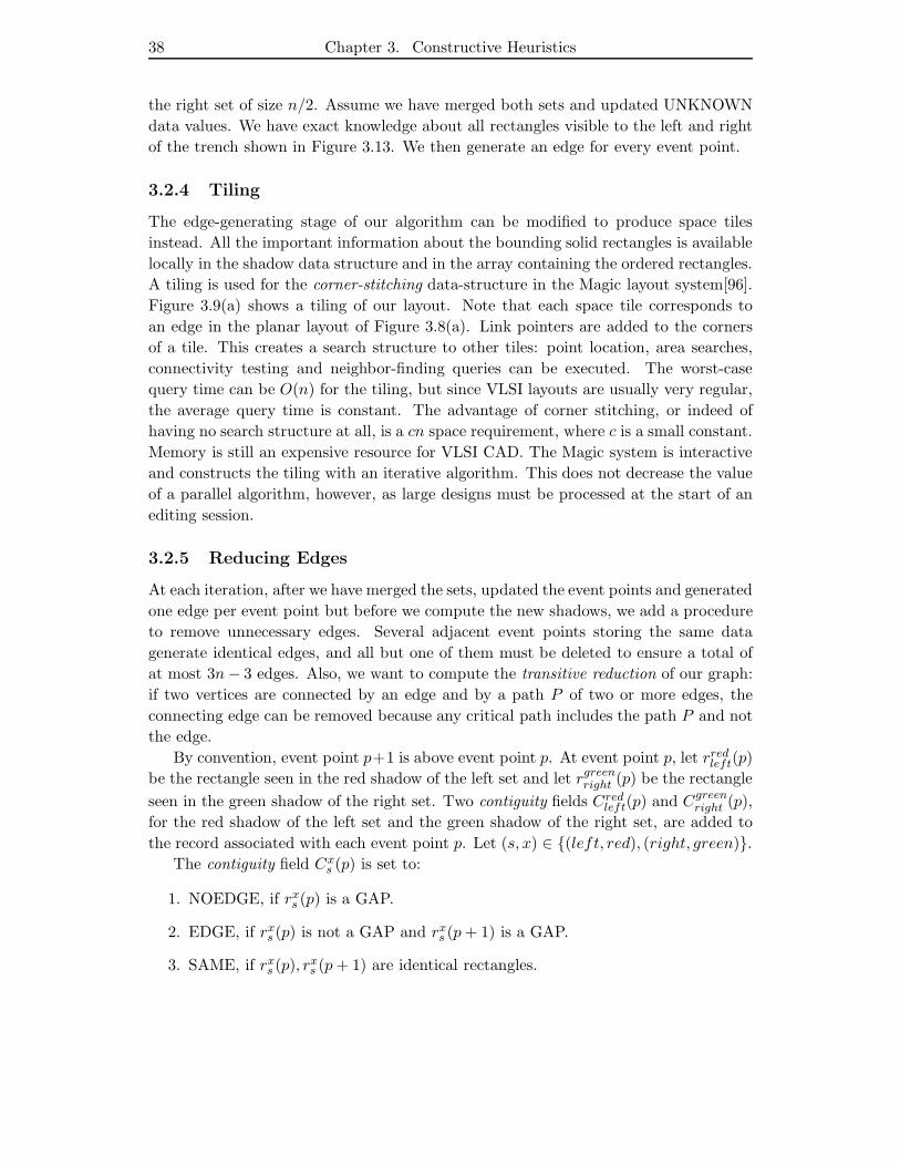
38 Chapter 3. Constructive Heuristics
the right set of size n/2. Assume we have merged both sets and updated UNKNOWN
data values. We have exact knowledge about all rectangles visible to the left and right
of the trench shown in Figure 3.13. We then generate an edge for every event point.
3.2.4 Tiling
The edge-generating stage of our algorithm can be modified to produce space tiles
instead. All the important information about the bounding solid rectangles is available
locally in the shadow data structure and in the array containing the ordered rectangles.
A tiling is used for the corner-stitching data-structure in the Magic layout system[96].
Figure 3.9(a) shows a tiling of our layout. Note that each space tile corresponds to
an edge in the planar layout of Figure 3.8(a). Link pointers are added to the corners
of a tile. This creates a search structure to other tiles: point location, area searches,
connectivity testing and neighbor-finding queries can be executed. The worst-case
query time can be O(n) for the tiling, but since VLSI layouts are usually very regular,
the average query time is constant. The advantage of corner stitching, or indeed of
having no search structure at all, is a cn space requirement, where c is a small constant.
Memory is still an expensive resource for VLSI CAD. The Magic system is interactive
and constructs the tiling with an iterative algorithm. This does not decrease the value
of a parallel algorithm, however, as large designs must be processed at the start of an
editing session.
3.2.5 Reducing Edges
At each iteration, after we have merged the sets, updated the event points and generated
one edge per event point but before we compute the new shadows, we add a procedure
to remove unnecessary edges. Several adjacent event points storing the same data
generate identical edges, and all but one of them must be deleted to ensure a total of
at most 3n − 3 edges. Also, we want to compute the transitive reduction of our graph:
if two vertices are connected by an edge and by a path P of two or more edges, the
connecting edge can be removed because any critical path includes the path P and not
the edge.
By convention, event point p+1 is above event point p. At event point p, let rredleft(p)
be the rectangle seen in the red shadow of the left set and let rgreenright (p) be the rectangle
seen in the green shadow of the right set. Two contiguity fields Credleft(p) and Cgreen
right (p),
for the red shadow of the left set and the green shadow of the right set, are added to
the record associated with each event point p. Let (s, x) ∈ (left, red), (right, green).The contiguity field Cx
s (p) is set to:
1. NOEDGE, if rxs (p) is a GAP.
2. EDGE, if rxs (p) is not a GAP and rx
s (p + 1) is a GAP.
3. SAME, if rxs (p), rx
s (p + 1) are identical rectangles.
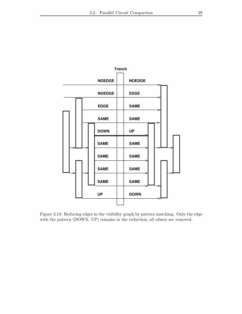
3.2. Parallel Circuit Compaction 39
Trench
UP DOWN
SAME SAME
SAME SAME
SAME SAME
SAME SAME
DOWN UP
SAME
EDGE
NOEDGE
SAME SAME
EDGE
NOEDGE
NOEDGE
Figure 3.13: Reducing edges in the visibility graph by pattern matching. Only the edgewith the pattern (DOWN, UP) remains in the reduction; all others are removed.
40 Chapter 3. Constructive Heuristics
4. UP, if rxs (p), rx
s (p + 1) are different rectangles and there is a path from rxs (p) to
rxs (p + 1).
5. DOWN, if rxs (p), rx
s (p+1) are different rectangles and there is a path from rxs (p+1)
to rxs (p).
Note that it can be determined in constant time whether there is a directed path from
rxs (p) to rx
s (p + 1): the y-ranges of the two rectangles overlap, and the x-coordinate of
rxs (p) is less than the x-coordinate of rx
s (p+1). If the rectangles do not overlap, another
rectangle or GAP is visible in the shadow. A similar argument applies for finding paths
from rxs (p + 1) to rx
s (p).
We compute the contiguity value pairs (Credleft(p), Cgreen
right (p)) at every event point p
and apply to the resulting patterns a procedure to remove edges not in the transitive
reduction.
To illustrate the pattern-matching procedure, consider the examples in Figure 3.13.
Only the edge with the pattern (DOWN, UP) remains in the reduction; all others are
removed.
Ex. 1 The pattern (UP, DOWN) implies that there is a path from rectangle rredleft(p) to
rredleft(p+1), an edge crosses the “trench” at the edge at p+1, and there is a path
from rgreenright (p + 1) to rgreen
right (p). Therefore the pattern (UP, DOWN) indicates
that the edge at p can be removed.
Ex. 2 All edges with the pattern (SAME, SAME) can be removed.
Ex. 3 The two edges with a pattern that contains NOEDGE can be removed.
Ex. 4 The pattern (DOWN, UP) implies that there is a path from rectangle rredleft(p+1)
to rredleft(p), an edge crosses the “trench” at the edge at p, and there is a path
from rgreenright (p) to rgreen
right (p + 1). Therefore the set of two edges with the pattern
(SAME, SAME) followed by (EDGE, SAME) can be removed.
From each of the 25 resulting patterns we can deduce locally whether to delete the
edge at p or the edge p + 1:
(a) Patterns on which no action is taken are: (UP, UP), (DOWN, DOWN), and any
pattern containing EDGE but not NOEDGE.
(b) Patterns removing the edge at p are: (SAME, SAME), (SAME, DOWN), (UP,
SAME), (UP, DOWN), and any pattern containing NOEDGE.
(c) Patterns removing the edge at p + 1 are: (DOWN, SAME), (SAME, UP) and
(DOWN, UP).
3.2. Parallel Circuit Compaction 41
The patterns that remove the edge at p + 1 need special attention. A sequence of
(SAME, SAME) patterns at pi and higher event points followed by any other pattern
at pj generates a set of equivalent edges at pi through pj, as can be seen in Figure 3.13.
If the pattern at pi−1 deletes the edge at pi, the whole set including the edge at pj must
be deleted. This is done by another prefix computation that copies a “delete-edge” flag
from the lowest event point pi in the sequence of (SAME, SAME) patterns to all other
event points pi, . . . , pj in the sequence.
Lemma 8 The above pattern-matching procedure computes the transitive reduction of
an interval dag.
Proof We show that when an edge is in the transitive reduction, the pattern-matching
procedure does not remove it, and that when an edge is not in the transitive reduction,
the pattern-matching procedure removes it.
Case (a) Only edges not in the transitive reduction are removed. As explained
above, this is shown by checking all 25 patterns. The patterns remove an edge between
rectangles rredleft(p), rgreen
right (p) only when there is also a path from rectangle rredleft(p) to
rgreenright (p).
Case (b) Only edges in the transitive reduction remain. Assume that after the
application of the above pattern-matching procedure there is an edge at p between
rectangles rredleft(p), rgreen
right (p) that is not in the transitive reduction. Therefore there is
a path P from rredleft(p) to rgreen
right (p). Without loss of generality, assume the path P runs
in the planar graph above the edge at p. Consider the iteration when the edge at p was
created. Because there is a path P from rredleft(p) to rgreen
right (p) crossing the trench above
p, the possible patterns at event point p are: (UP, DOWN), (SAME, DOWN), (UP,
SAME), (SAME, SAME), but all these patterns remove edge p, a contradiction. 2
The above pattern-matching procedure completes our algorithm for computing the
transitive reduction of an interval dag.
3.2.6 Complexity Analysis
The preprocessing consists of sorting the rectangles by their x-coordinates, which can
be done in time O(log2 n) time on a O(n/log n) EREW PRAM[10]. As our algorithm
is recursive, it takes log n iterations, so each iteration must work in time O(log n)
with O(n/log n) processors. The local and parallel prefix algorithms run within these
bounds, and the recursion imposes no scheduling overhead.
Theorem 5 A compaction constraint graph that corresponds to the transitive reduction
of an interval dag can be computed from the rectangle representation in O(log2 n) time
on a O(n/log n) EREW PRAM.
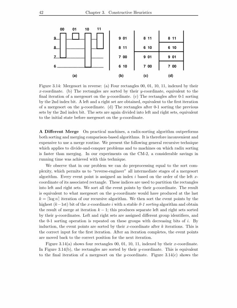
42 Chapter 3. Constructive Heuristics
6
7
8
9 9 01
8 11
7 00
6 10
00 01 10 11
9 01
8 11
7 00
6 10
9 01
8 11
7 00
6 10
(a) (b) (c) (d)
Figure 3.14: Mergesort in reverse: (a) Four rectangles 00, 01, 10, 11, indexed by theirx-coordinate. (b) The rectangles are sorted by their y-coordinate, equivalent to thefinal iteration of a mergesort on the y-coordinate. (c) The rectangles after 0-1 sortingby the 2nd index bit. A left and a right set are obtained, equivalent to the first iterationof a mergesort on the y-coordinate. (d) The rectangles after 0-1 sorting the previoussets by the 2nd index bit. The sets are again divided into left and right sets, equivalentto the initial state before mergesort on the y-coordinate.
A Different Merge On practical machines, a radix-sorting algorithm outperforms
both sorting and merging comparison-based algorithms. It is therefore inconvenient and
expensive to use a merge routine. We present the following general recursive technique
which applies to divide-and-conquer problems and to machines on which radix sorting
is faster than merging. In our experiments on the CM-2, a considerable savings in
running time was achieved with this technique.
We observe that in our problem we can do preprocessing equal to the sort com-
plexity, which permits us to “reverse-engineer” all intermediate stages of a mergesort
algorithm. Every event point is assigned an index i based on the order of the left x-
coordinate of its associated rectangle. These indices are used to partition the rectangles
into left and right sets. We sort all the event points by their y-coordinate. The result
is equivalent to what mergesort on the y-coordinate would have produced at the last
k = ⌈log n⌉ iteration of our recursive algorithm. We then sort the event points by the
highest (k−1st) bit of the x-coordinate i with a stable 0-1 sorting algorithm and obtain
the result of merge at iteration k − 1; this produces separate left and right sets sorted
by their y-coordinates. Left and right sets are assigned different group identifiers, and
the 0-1 sorting operation is repeated on these groups with decreasing bits of i. By
induction, the event points are sorted by their x-coordinate after k iterations. This is
the correct input for the first iteration. After an iteration completes, the event points
are moved back to the correct position for the next iteration.
Figure 3.14(a) shows four rectangles 00, 01, 10, 11, indexed by their x-coordinate.
In Figure 3.14(b), the rectangles are sorted by their y-coordinate. This is equivalent
to the final iteration of a mergesort on the y-coordinate. Figure 3.14(c) shows the
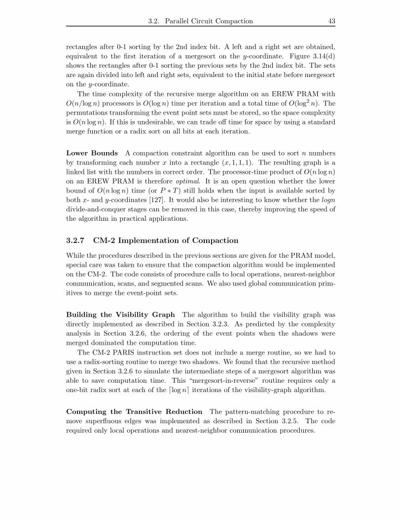
3.2. Parallel Circuit Compaction 43
rectangles after 0-1 sorting by the 2nd index bit. A left and a right set are obtained,
equivalent to the first iteration of a mergesort on the y-coordinate. Figure 3.14(d)
shows the rectangles after 0-1 sorting the previous sets by the 2nd index bit. The sets
are again divided into left and right sets, equivalent to the initial state before mergesort
on the y-coordinate.
The time complexity of the recursive merge algorithm on an EREW PRAM with
O(n/log n) processors is O(log n) time per iteration and a total time of O(log2 n). The
permutations transforming the event point sets must be stored, so the space complexity
is O(n log n). If this is undesirable, we can trade off time for space by using a standard
merge function or a radix sort on all bits at each iteration.
Lower Bounds A compaction constraint algorithm can be used to sort n numbers
by transforming each number x into a rectangle (x, 1, 1, 1). The resulting graph is a
linked list with the numbers in correct order. The processor-time product of O(n log n)
on an EREW PRAM is therefore optimal. It is an open question whether the lower
bound of O(n log n) time (or P ∗ T ) still holds when the input is available sorted by
both x- and y-coordinates [127]. It would also be interesting to know whether the logn
divide-and-conquer stages can be removed in this case, thereby improving the speed of
the algorithm in practical applications.
3.2.7 CM-2 Implementation of Compaction
While the procedures described in the previous sections are given for the PRAM model,
special care was taken to ensure that the compaction algorithm would be implemented
on the CM-2. The code consists of procedure calls to local operations, nearest-neighbor
communication, scans, and segmented scans. We also used global communication prim-
itives to merge the event-point sets.
Building the Visibility Graph The algorithm to build the visibility graph was
directly implemented as described in Section 3.2.3. As predicted by the complexity
analysis in Section 3.2.6, the ordering of the event points when the shadows were
merged dominated the computation time.
The CM-2 PARIS instruction set does not include a merge routine, so we had to
use a radix-sorting routine to merge two shadows. We found that the recursive method
given in Section 3.2.6 to simulate the intermediate steps of a mergesort algorithm was
able to save computation time. This “mergesort-in-reverse” routine requires only a
one-bit radix sort at each of the ⌈log n⌉ iterations of the visibility-graph algorithm.
Computing the Transitive Reduction The pattern-matching procedure to re-
move superfluous edges was implemented as described in Section 3.2.5. The code
required only local operations and nearest-neighbor communication procedures.
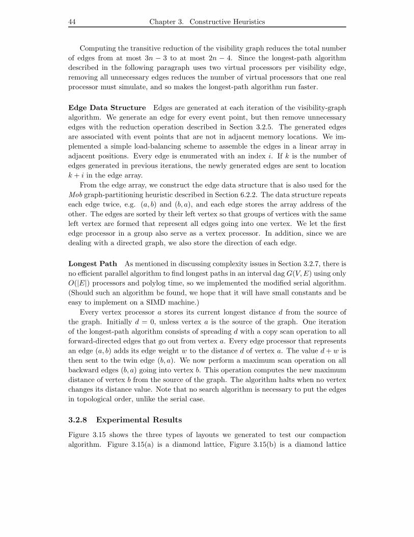
44 Chapter 3. Constructive Heuristics
Computing the transitive reduction of the visibility graph reduces the total number
of edges from at most 3n − 3 to at most 2n − 4. Since the longest-path algorithm
described in the following paragraph uses two virtual processors per visibility edge,
removing all unnecessary edges reduces the number of virtual processors that one real
processor must simulate, and so makes the longest-path algorithm run faster.
Edge Data Structure Edges are generated at each iteration of the visibility-graph
algorithm. We generate an edge for every event point, but then remove unnecessary
edges with the reduction operation described in Section 3.2.5. The generated edges
are associated with event points that are not in adjacent memory locations. We im-
plemented a simple load-balancing scheme to assemble the edges in a linear array in
adjacent positions. Every edge is enumerated with an index i. If k is the number of
edges generated in previous iterations, the newly generated edges are sent to location
k + i in the edge array.
From the edge array, we construct the edge data structure that is also used for the
Mob graph-partitioning heuristic described in Section 6.2.2. The data structure repeats
each edge twice, e.g. (a, b) and (b, a), and each edge stores the array address of the
other. The edges are sorted by their left vertex so that groups of vertices with the same
left vertex are formed that represent all edges going into one vertex. We let the first
edge processor in a group also serve as a vertex processor. In addition, since we are
dealing with a directed graph, we also store the direction of each edge.
Longest Path As mentioned in discussing complexity issues in Section 3.2.7, there is
no efficient parallel algorithm to find longest paths in an interval dag G(V,E) using only
O(|E|) processors and polylog time, so we implemented the modified serial algorithm.
(Should such an algorithm be found, we hope that it will have small constants and be
easy to implement on a SIMD machine.)
Every vertex processor a stores its current longest distance d from the source of
the graph. Initially d = 0, unless vertex a is the source of the graph. One iteration
of the longest-path algorithm consists of spreading d with a copy scan operation to all
forward-directed edges that go out from vertex a. Every edge processor that represents
an edge (a, b) adds its edge weight w to the distance d of vertex a. The value d + w is
then sent to the twin edge (b, a). We now perform a maximum scan operation on all
backward edges (b, a) going into vertex b. This operation computes the new maximum
distance of vertex b from the source of the graph. The algorithm halts when no vertex
changes its distance value. Note that no search algorithm is necessary to put the edges
in topological order, unlike the serial case.
3.2.8 Experimental Results
Figure 3.15 shows the three types of layouts we generated to test our compaction
algorithm. Figure 3.15(a) is a diamond lattice, Figure 3.15(b) is a diamond lattice
3.2. Parallel Circuit Compaction 45
Figure 3.15: Three uncompacted layouts with O(√
n) critical paths: (a) diamond lat-tice, (b) irregular diamond lattice, (c) irregular mesh.
Figure 3.16: Irregular diamond lattice. (a) Before compaction. (b) After compaction.
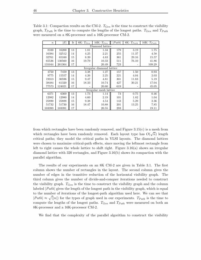
46 Chapter 3. Constructive Heuristics
Table 3.1: Compaction results on the CM-2. TGen is the time to construct the visibilitygraph, TPath is the time to compute the lengths of the longest paths. TGen and TPath
were measured on a 8K-processor and a 16K-processor CM-2.
n |E| It 8K: TGen 16K: TGen |Path| 8K: TPath 16K: TPath
Diamond lattice
8100 16200 13 1.81 1.34 179 3.19 1.7516384 32512 14 4.25 2.21 255 11.37 4.5832761 65160 15 8.39 4.83 361 29.16 15.5765536 130560 16 19.79 10.33 511 76.10 41.86
131044 261364 17 - 20.49 723 - 109.29
Irregular diamond lattice
4750 7459 13 3.38 1.27 157 1.50 0.939775 15557 14 4.26 2.25 221 4.04 2.03
19313 30596 15 9.47 4.81 301 11.83 5.1938484 61320 16 18.33 10.74 427 30.21 17.0477573 124021 17 - 20.60 619 - 45.05
Irregular mesh lattice
6371 6369 13 1.73 1.14 73 0.75 0.4612982 12980 14 4.60 2.19 101 1.82 1.0425890 25888 15 9.38 4.54 143 5.29 2.3651732 51730 16 18.47 10.88 201 13.25 7.85
103393 103391 17 - 20.55 293 - 19.11
from which rectangles have been randomly removed, and Figure 3.15(c) is a mesh from
which rectangles have been randomly removed. Each layout type has O(√
n) length
critical paths; they model the critical paths in VLSI layouts. The diamond lattices
were chosen to maximize critical-path effects, since moving the leftmost rectangle from
left to right causes the whole lattice to shift right. Figure 3.16(a) shows an irregular
diamond lattice with 320 rectangles, and Figure 3.16(b) shows its compaction with the
parallel algorithm.
The results of our experiments on an 8K CM-2 are given in Table 3.1. The first
column shows the number of rectangles in the layout. The second column gives the
number of edges in the transitive reduction of the horizontal visibility graph. The
third column gives the number of divide-and-conquer iterations needed to construct
the visibility graph. TGen is the time to construct the visibility graph and the column
labeled |Path| gives the length of the longest path in the visibility graph, which is equal
to the number of iterations of the longest-path algorithm used here. We can see that
|Path| ≈√
(|n|) for the types of graph used in our experiments. TPath is the time to
compute the lengths of the longest paths. TGen and TPath were measured on both an
8K-processor and a 16K-processor CM-2.
We find that the complexity of the parallel algorithm to construct the visibility
3.2. Parallel Circuit Compaction 47
graph of n rectangles is O(log2 n) with O(n log n) processors, as predicted in Sec-
tion 3.2.6. Every time we double the number of rectangles in the layout, the compu-
tation time increases by slightly more than twice, since the number of iterations in
the divide-and-conquer algorithm increases by one. Doubling the number of processors
reduces the computation time by half. Depending on layout size, this holds for ratios
of virtual to real processors ranging from 1 to 32, so we can deduce that the algorithm
exhibits speedup linear in the number of processors.
We also found that the measured running times of the O(√
n) longest-path al-
gorithm were within an order of magnitude of the running times for the O(log2 n)
visibility-graph algorithm. Only for the examples in which n < 105 does the fact that
its asymptotic behavior is not polylogarithmic finally catch up with the longest-path
algorithm.

49
Chapter 4
Local Search Heuristics for VLSI
Placement
4.1 Local Search Heuristics
Local search heuristics have been established as the method of choice in many opti-
mization problems whenever very good solutions are desired. In local search heuristics,
an initial solution S1 is constructed, usually by some random procedure, and a cost
function f is computed. Changes are made to the current solution and a new solution
S2, which we say is in the neighborhood of the current solution, replaces the current
solution. The improvement in the cost function f obtained from changing from solution
S1 to solution S2 is given by the gain function ∆f := f(S1) − f(S2). A positive gain
change is one that decreases cost. The termination rules differ for each heuristic.
The procedure that generates changes to the current solution defines a neighborhood
whose structure depends on the problem being solved. We define neighborhoods for
graph partitioning, graph embedding, and column-conflict minimization for channel
routing in Sections 4.3,4.4, and 4.5.
Classical local search heuristics for graph embedding are steepest descent, the Kernig-
han-Lin heuristic (KL)[68], Fiduccia-Mattheyses (FM)[47] heuristic, and simulated an-
nealing (SA)[69]. The Kernighan-Lin heuristic and the Fiduccia-Mattheyses heuristic
are mainly graph-partitioning heuristics and are introduced in Section 4.3.
4.1.1 Steepest Descent
The steepest-descent heuristic selects a neighboring solution that gives the largest de-
crease in cost if accepted. If this decrease is positive, the new solution is accepted;
otherwise the heuristic halts. This heuristic tends to become trapped in bad local
minima, and is not widely used since better local search heuristics are available.
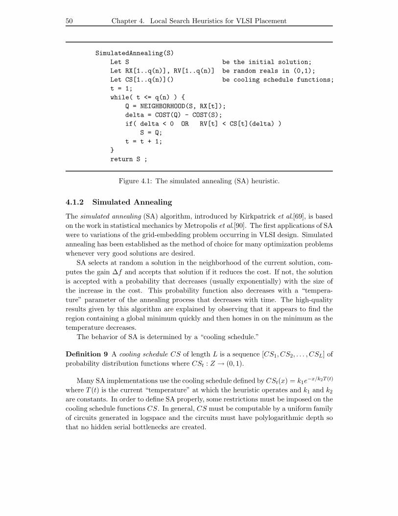
50 Chapter 4. Local Search Heuristics for VLSI Placement
SimulatedAnnealing(S)
Let S be the initial solution;
Let RX[1..q(n)], RV[1..q(n)] be random reals in (0,1);
Let CS[1..q(n)]() be cooling schedule functions;
t = 1;
while( t <= q(n) )
Q = NEIGHBORHOOD(S, RX[t]);
delta = COST(Q) - COST(S);
if( delta < 0 OR RV[t] < CS[t](delta) )
S = Q;
t = t + 1;
return S ;
Figure 4.1: The simulated annealing (SA) heuristic.
4.1.2 Simulated Annealing
The simulated annealing (SA) algorithm, introduced by Kirkpatrick et al.[69], is based
on the work in statistical mechanics by Metropolis et al.[90]. The first applications of SA
were to variations of the grid-embedding problem occurring in VLSI design. Simulated
annealing has been established as the method of choice for many optimization problems
whenever very good solutions are desired.
SA selects at random a solution in the neighborhood of the current solution, com-
putes the gain ∆f and accepts that solution if it reduces the cost. If not, the solution
is accepted with a probability that decreases (usually exponentially) with the size of
the increase in the cost. This probability function also decreases with a “tempera-
ture” parameter of the annealing process that decreases with time. The high-quality
results given by this algorithm are explained by observing that it appears to find the
region containing a global minimum quickly and then homes in on the minimum as the
temperature decreases.
The behavior of SA is determined by a “cooling schedule.”
Definition 9 A cooling schedule CS of length L is a sequence [CS1, CS2, . . . , CSL] of
probability distribution functions where CSt : Z → (0, 1).
Many SA implementations use the cooling schedule defined by CSt(x) = k1e−x/k2T (t)
where T (t) is the current “temperature” at which the heuristic operates and k1 and k2
are constants. In order to define SA properly, some restrictions must be imposed on the
cooling schedule functions CS. In general, CS must be computable by a uniform family
of circuits generated in logspace and the circuits must have polylogarithmic depth so
that no hidden serial bottlenecks are created.

4.1. Local Search Heuristics 51
We can now explicitly define the SA heuristic, outlined in pseudocode in Figure 4.1.
We assume that q(n), the number of steps it executes, is polynomial in the number n
of vertices. The probabilistic nature of SA is reflected in sets RX, RV of q(n) random
variables that are real numbers selected uniformly and independently from the interval
(0, 1). A random variable uniformly distributed over the interval (0, 1) is less than or
equal to p with probability p, assuming 0 ≤ p ≤ 1.
The functions NEIGHBORHOOD() and COST() are defined by the problem to be solved.
SA randomly selects a solution Q with the function NEIGHBORHOOD(S, RX[t]). The
change ∆ in the cost is computed and Q replaces the current working solution S if
the cost decreases or if the current probability distribution RVt < CSt(∆). The SA
heuristic keeps exploring the neighborhood of its working solution P until the time
limit q(n) is exceeded.
We show in Section 5.1.2 that a version of SA called the “zero-temperature” version,
ZT-SA, is P-hard for the graph-partitioning problem. We now define ZT-SA.
Definition 10 The zero-temperature version of SA (ZT-SA) uses a cooling schedule
CS for which RVt < CSt(∆) is always false.
In this version of SA, only improving solutions are accepted. When the standard
cooling schedule CSt(x) = k1e−x/k2T (t) is used, this is equivalent to operating at zero
temperature. While there is no uniform distribution on infinite sets, namely the set
of integers Z, note that CSt has a finite domain because the difference in bisection
widths between any two partitions is bounded. ZT-SA is a form of probabilistic
steepest-descent algorithm. In practice, SA always enters a low-temperature phase,
which implies that if it enters this phase with a partition that is not locally optimal,
the problem is likely to be very hard to parallelize.
4.1.3 Convergence of Simulated Annealing
Geman and Geman[50], Lundy and Mees[87], and Mitra et al.[91] have shown by
Markov chain analysis that SA with a logarithmic cooling schedule converges to the
optimal solution in time O(an), a > 1. Worst-case examples can be constructed that
put a lower bound of Ω(an) on SA’s running time. SA can actually run more slowly
than the naive algorithm that simply searches the whole solution space.
The result by Geman and Geman was initially derived for an application of SA
to image processing, whereas the other two papers address the general case. For the
analysis of Lundy and Mees and Mitra et al. to hold, certain weak conditions must be
met:
(a) The initial solution can be generated in polynomial time.
(b) The transformation of one solution into a neighboring solution can be done in
polynomial time.

52 Chapter 4. Local Search Heuristics for VLSI Placement
(c) A polynomial number of transformations suffices to transform one solution into
any other solution.
(d) The cost function f and the gain function ∆f must be computable in polynomial
time.
There is overwhelming empirical evidence that SA provides excellent solutions for
most problem instances in polynomial time, but no theoretical work exists to back
up these results. Often the results cited above showing convergence in O(an) time
are invoked to justify convergence in polynomial time, although no proofs of this are
known. More research needs to be done to explain SA’s convergence behavior with fast
cooling schedules. An encouraging result is Sorkin’s showing that SA with a fast cooling
schedule converges on a fractal landscape[131]. He conjectures that the neighborhood
structure of VLSI placement problems may have fractal properties.
4.2 Parallel Local Search
Greening[55] gives a survey of parallel simulated-annealing techniques and classifies
parallel local search algorithms into two categories: perfect convergence algorithms
that emulate the execution of a serial algorithm, and altered convergence algorithms
that allow for errors when accepting moves.
The simplicity of the SA algorithm seems to make an implementation on a massively
parallel computer almost trivial. It is therefore surprising that the goal of parallelizing
SA by straightforward or elaborate means has eluded researchers, and is in fact (as
shown in Chapter 5) impossible for some problems in the worst case.
A parallel local search heuristic computes cost and gain functions once per iteration,
independently of how many elements are selected for moves or swaps. It is therefore
desirable for computational efficiency to move a set of elements on each iteration.
Every element can decide whether to move or not on the basis of the gain function ∆f .
However, for most problems in which local search is used, the sum of the gain functions
only approximates the quality of a resulting solution. The gains may not take fully
into account that other elements are moving at the same time. This is the reason that
local search is difficult to parallelize: parallel moves introduce errors in the cost and
gain functions, and thus can produce results not produced by the serial local search
heuristic.
4.2.1 Perfect Convergence Algorithms
Perfect convergence algorithms attempt to emulate the execution of a serial algorithm,
usually by trying to make exact the parallel computations of gain functions. A parallel
local search heuristic that behaves differently from its serial equivalent cannot rely on
experimental work showing good convergence in polynomial time with one processor.
The proofs of SA’s convergence (with the SWAP neighborhood) to an optimal solution
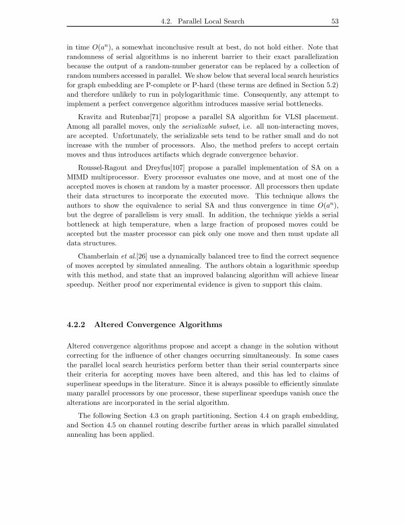
4.2. Parallel Local Search 53
in time O(an), a somewhat inconclusive result at best, do not hold either. Note that
randomness of serial algorithms is no inherent barrier to their exact parallelization
because the output of a random-number generator can be replaced by a collection of
random numbers accessed in parallel. We show below that several local search heuristics
for graph embedding are P-complete or P-hard (these terms are defined in Section 5.2)
and therefore unlikely to run in polylogarithmic time. Consequently, any attempt to
implement a perfect convergence algorithm introduces massive serial bottlenecks.
Kravitz and Rutenbar[71] propose a parallel SA algorithm for VLSI placement.
Among all parallel moves, only the serializable subset, i.e. all non-interacting moves,
are accepted. Unfortunately, the serializable sets tend to be rather small and do not
increase with the number of processors. Also, the method prefers to accept certain
moves and thus introduces artifacts which degrade convergence behavior.
Roussel-Ragout and Dreyfus[107] propose a parallel implementation of SA on a
MIMD multiprocessor. Every processor evaluates one move, and at most one of the
accepted moves is chosen at random by a master processor. All processors then update
their data structures to incorporate the executed move. This technique allows the
authors to show the equivalence to serial SA and thus convergence in time O(an),
but the degree of parallelism is very small. In addition, the technique yields a serial
bottleneck at high temperature, when a large fraction of proposed moves could be
accepted but the master processor can pick only one move and then must update all
data structures.
Chamberlain et al.[26] use a dynamically balanced tree to find the correct sequence
of moves accepted by simulated annealing. The authors obtain a logarithmic speedup
with this method, and state that an improved balancing algorithm will achieve linear
speedup. Neither proof nor experimental evidence is given to support this claim.
4.2.2 Altered Convergence Algorithms
Altered convergence algorithms propose and accept a change in the solution without
correcting for the influence of other changes occurring simultaneously. In some cases
the parallel local search heuristics perform better than their serial counterparts since
their criteria for accepting moves have been altered, and this has led to claims of
superlinear speedups in the literature. Since it is always possible to efficiently simulate
many parallel processors by one processor, these superlinear speedups vanish once the
alterations are incorporated in the serial algorithm.
The following Section 4.3 on graph partitioning, Section 4.4 on graph embedding,
and Section 4.5 on channel routing describe further areas in which parallel simulated
annealing has been applied.
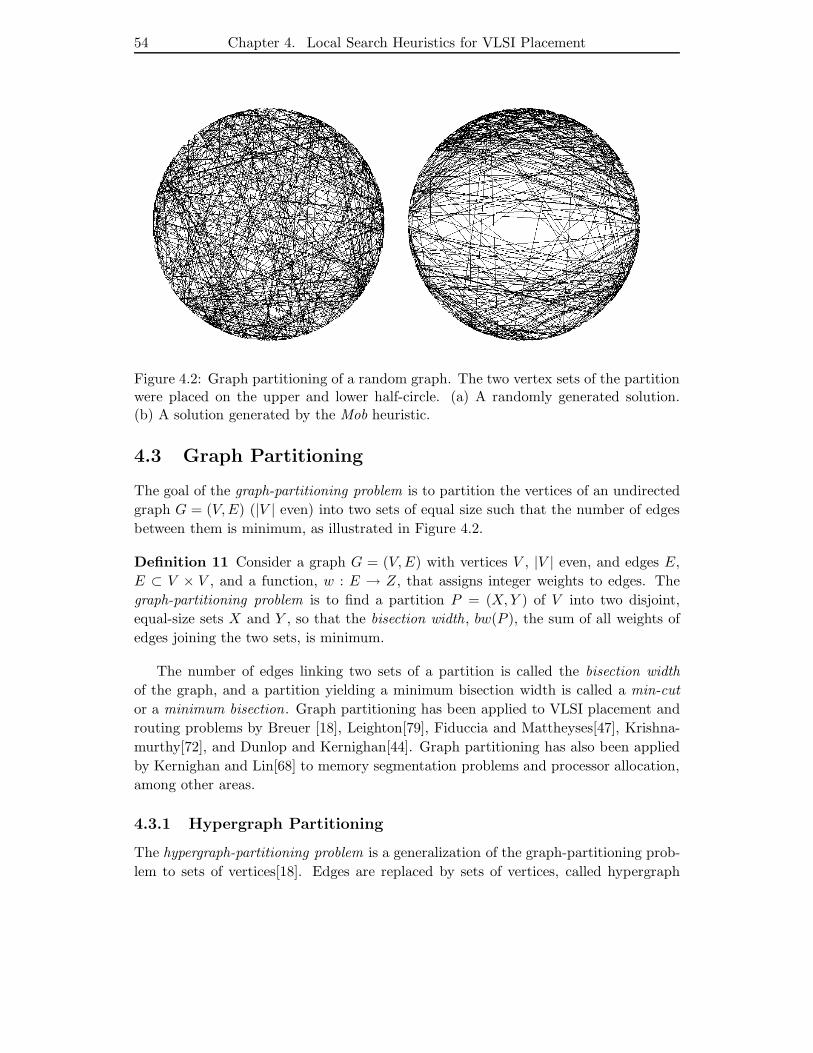
54 Chapter 4. Local Search Heuristics for VLSI Placement
Figure 4.2: Graph partitioning of a random graph. The two vertex sets of the partitionwere placed on the upper and lower half-circle. (a) A randomly generated solution.(b) A solution generated by the Mob heuristic.
4.3 Graph Partitioning
The goal of the graph-partitioning problem is to partition the vertices of an undirected
graph G = (V,E) (|V | even) into two sets of equal size such that the number of edges
between them is minimum, as illustrated in Figure 4.2.
Definition 11 Consider a graph G = (V,E) with vertices V , |V | even, and edges E,
E ⊂ V × V , and a function, w : E → Z, that assigns integer weights to edges. The
graph-partitioning problem is to find a partition P = (X,Y ) of V into two disjoint,
equal-size sets X and Y , so that the bisection width, bw(P ), the sum of all weights of
edges joining the two sets, is minimum.
The number of edges linking two sets of a partition is called the bisection width
of the graph, and a partition yielding a minimum bisection width is called a min-cut
or a minimum bisection. Graph partitioning has been applied to VLSI placement and
routing problems by Breuer [18], Leighton[79], Fiduccia and Mattheyses[47], Krishna-
murthy[72], and Dunlop and Kernighan[44]. Graph partitioning has also been applied
by Kernighan and Lin[68] to memory segmentation problems and processor allocation,
among other areas.
4.3.1 Hypergraph Partitioning
The hypergraph-partitioning problem is a generalization of the graph-partitioning prob-
lem to sets of vertices[18]. Edges are replaced by sets of vertices, called hypergraph
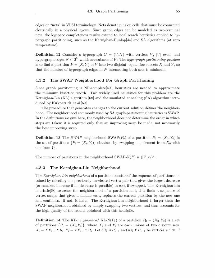
4.3. Graph Partitioning 55
edges or “nets” in VLSI terminology. Nets denote pins on cells that must be connected
electrically in a physical layout. Since graph edges can be modeled as two-terminal
nets, the logspace completeness results extend to local search heuristics applied to hy-
pergraph partitioning, such as the Kernighan-Dunlop[44] and SA algorithms (at zero
temperature).
Definition 12 Consider a hypergraph G = (V,N) with vertices V , |V | even, and
hypergraph edges N ⊂ 2V which are subsets of V . The hypergraph-partitioning problem
is to find a partition P = (X,Y ) of V into two disjoint, equal-size subsets X and Y , so
that the number of hypergraph edges in N intersecting both sets is minimum.
4.3.2 The SWAP Neighborhood For Graph Partitioning
Since graph partitioning is NP-complete[49], heuristics are needed to approximate
the minimum bisection width. Two widely used heuristics for this problem are the
Kernighan-Lin (KL) algorithm [68] and the simulated annealing (SA) algorithm intro-
duced by Kirkpatrick et al.[69].
The procedure that generates changes to the current solution defines the neighbor-
hood. The neighborhood commonly used by SA graph-partitioning heuristics is SWAP.
In the definitions we give here, the neighborhood does not determine the order in which
steps are taken; it is required only that an improving swap be made, not necessarily
the best improving swap.
Definition 13 The SWAP neighborhood SWAP(P0) of a partition P0 = (X0, Y0) is
the set of partitions Pi = (Xi, Yi) obtained by swapping one element from X0 with
one from Y0.
The number of partitions in the neighborhood SWAP-N(P ) is (|V |/2)2 .
4.3.3 The Kernighan-Lin Neighborhood
The Kernighan-Lin neighborhood of a partition consists of the sequence of partitions ob-
tained by selecting one previously unselected vertex pair that gives the largest decrease
(or smallest increase if no decrease is possible) in cost if swapped. The Kernighan-Lin
heuristic[68] searches the neighborhood of a partition and, if it finds a sequence of
vertex swaps that gives a smaller cost, replaces the current partition by the new one
and continues. If not, it halts. The Kernighan-Lin neighborhood is larger than the
SWAP neighborhood obtained by simply swapping two vertices, and thus accounts for
the high quality of the results obtained with this heuristic.
Definition 14 The KL-neighborhood KL-N(P0) of a partition P0 = (X0, Y0) is a set
of partitions Pi = (Xi, Yi), where Xi and Yi are each unions of two disjoint sets:
Xi = XFi ∪XRi, Yi = Y Fi ∪Y Ri. Let a ∈ XRi−1 and b ∈ Y Ri−1 be vertices which, if
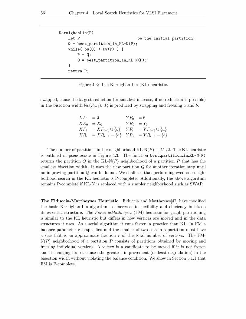
56 Chapter 4. Local Search Heuristics for VLSI Placement
KernighanLin(P)
Let P be the initial partition;
Q = best_partition_in_KL-N(P);
while( bw(Q) < bw(P) )
P = Q;
Q = best_partition_in_KL-N(P);
return P;
Figure 4.3: The Kernighan-Lin (KL) heuristic.
swapped, cause the largest reduction (or smallest increase, if no reduction is possible)
in the bisection width bw(Pi−1). Pi is produced by swapping and freezing a and b:
XF0 = ∅ Y F0 = ∅XR0 = X0 Y R0 = Y0
XFi = XFi−1 ∪ b Y Fi = Y Fi−1 ∪ aXRi = XRi−1 − a Y Ri = Y Ri−1 − b
The number of partitions in the neighborhood KL-N(P ) is |V |/2. The KL heuristic
is outlined in pseudocode in Figure 4.3. The function best partition in KL-N(P)
returns the partition Q in the KL-N(P ) neighborhood of a partition P that has the
smallest bisection width. It uses the new partition Q for another iteration step until
no improving partition Q can be found. We shall see that performing even one neigh-
borhood search in the KL heuristic is P-complete. Additionally, the above algorithm
remains P-complete if KL-N is replaced with a simpler neighborhood such as SWAP.
The Fiduccia-Mattheyses Heuristic Fiduccia and Mattheyses[47] have modified
the basic Kernighan-Lin algorithm to increase its flexibility and efficiency but keep
its essential structure. The FiducciaMattheyses (FM) heuristic for graph partitioning
is similar to the KL heuristic but differs in how vertices are moved and in the data
structures it uses. As a serial algorithm it runs faster in practice than KL. In FM a
balance parameter r is specified and the smaller of two sets in a partition must have
a size that is an approximate fraction r of the total number of vertices. The FM-
N(P ) neighborhood of a partition P consists of partitions obtained by moving and
freezing individual vertices. A vertex is a candidate to be moved if it is not frozen
and if changing its set causes the greatest improvement (or least degradation) in the
bisection width without violating the balance condition. We show in Section 5.1.1 that
FM is P-complete.
4.4. Graph Embedding 57
4.3.4 The Complexity of Graph-Partitioning Algorithms
For the graph-partitioning problem, both Kernighan-Lin and simulated annealing give
excellent results on serial machines for random graphs of small degree and moderate
size[65,77]. The time for one run of KL from an initial partition is much smaller than
that for SA. However, KL generally gives bisection widths that are about 10% larger
than those provided by SA. When the running times of both are equalized by making
many more runs of KL with randomly chosen initial partitions and choosing the best
results of all runs, Johnson et al.[65] show that KL gives a best bisection width typically
within a few percent of SA’s best bisection width, although SA continues to provide
better results.
An important reason for introducing a new heuristic is that both KL and SA are
believed to be hard to parallelize. We have shown that KL is P-complete under logspace
reductions on graphs with unit-weight edges[120,121]. A randomized local search al-
gorithm, the zero-temperature version of SA, is shown in Section 5.1 to be P-hard
under logspace reductions. We also show in Section 5.1 that Mob is P-hard under some
restrictions, which occur only infrequently in practice.
In their study of local search, Johnson, Papadimitriou and Yannakakis [66] have
shown that a search of a single KL neighborhood is P-complete when graphs have
edge weights exponential in the size of a graph and the bisection size is defined to be
the sum of the weights of edges in a bisection. Our P-completeness result is obtained
for unit-weight edges. Schaffer and Yannakakis have independently shown that local
search on the SWAP neighborhood on unit-weight edge graphs is P-complete [126].
From this they deduce that an entire local search with KL of unit-weight edge graphs
is P-complete. Our result of completeness of KL for search of just one neighborhood
implies completeness of the entire search done by KL. Our proof of P-hardness of zero-
temperature SA implies P-completeness for deterministic local search heuristics using
the SWAP neighborhood.
Other heuristics for graph partitioning have been developed. Bui, Chaudhuri,
Leighton and Sipser[20,21] give a min-cut, max-flow-based algorithm to partition a
graph with unit edge weights. This algorithm works well with graphs of a particular
structure having small expected bisection widths, and it would be interesting to know
if it can be parallelized. Bui, Heigham, Jones and Leighton[22] use a maximum random
matching algorithm to coalesce nodes into pairs, thus forming a smaller graph of higher
average degree, and then run either KL or SA on this graph to obtain a partition. Ver-
tex pairs are then separated to create a partition for the original graph that is used as
an initial partition for either KL or SA.
4.4 Graph Embedding
In this section we give an overview of graph-embedding heuristics. Here the problem
is to embed a graph G = (V,E) into other graphs and structures. A cost function

58 Chapter 4. Local Search Heuristics for VLSI Placement
Figure 4.4: 16-to-1 grid embedding of a random graph: (a) A randomly generatedsolution. (b) A solution generated by the Mob heuristic.
Figure 4.5: 1-to-1 grid embedding of a random graph: (a) A randomly generatedsolution. (b) A solution generated by the Mob heuristic.
4.4. Graph Embedding 59
assigns a value to each embedding; the objective is to minimize that cost function, as
illustrated in Figures 4.4 and 4.5. We will call the target structure a network, and the
vertices of the target structure nodes.
Definition 15 Consider two graphs G1 = (V1, E1) and G2 = (V2, E2). An embedding
of G1 into G2 is a pair of mappings S = ν, ǫ where ν : V1 7→ V2 is a mapping of the
vertices V1 to the network nodes V2 and ǫ maps edges in G1 to paths in G2. Let Sbe the set of all graph embeddings S of G1 in G2. Let the cost function f : S 7→ Rassign a cost to each embedding in S. The graph-embedding problem is to find a graph
embedding S with minimum cost f(S).
We show in Section 5.1 that for graph partitioning, local search under the SWAP
neighborhood is P-hard. Using this result, we show in Section 5.2 that local search
heuristics for grid and hypercube embeddings are P-hard (evidence of non-parallelizability)
when the neighbors in the solution space are generated by swapping the embeddings
of two vertices[119,122]. We give two logspace constructions that map the graph used
in the graph-partitioning completeness proof into initial embeddings in the grid and
hypercube.
4.4.1 VLSI Placement and Minimization of Data Movement
Graph embedding finds application in VLSI placement and the minimization of data
movement in parallel computers. The VLSI-placement problem can be modeled by a
grid embedding that is restricted to allow only one logic element location per grid node.
Hypercube embeddings and grid embeddings are used to embed a data-structure graph
on the topology of a parallel machine. An automatic graph-embedding tool optimizes
communication resources, enhances fault tolerance, and allows parallel programs to be
divorced to some extent from the structure of the underlying communication network.
SIMD-style parallel machines, such as the Connection Machine and the MasPar Ma-
chines, are characterized by small processors (one to four bits per processing element)
that operate in lockstep when activated and a communication network with a high
latency unless nearest neighbors are accessed. Good code that makes efficient use of
the processors can be written with traditional editors, compilers and debuggers. How-
ever, the cost of communication is so high on these machines that it must be severely
controlled in order to obtain peak performance. One way to do this is to place tasks
on nodes in such a way as to minimize the cost of communication between nodes. In-
stead of always using message-passing primitives for data access, data can be referenced
across an edge by direct addressing if the connected vertex resides on the same proces-
sor. The graph-embedding algorithms considered in this paper have the potential of
dramatically cutting down on communication costs.
60 Chapter 4. Local Search Heuristics for VLSI Placement
4.4.2 Bulk Parallelism
An important paradigm for programming parallel machines is the bulk parallelism model
introduced by Valiant[136]. In this model, n virtual processors are simulated on a
computing network with (roughly) n/ log n real processors. The Connection Machine
software provides support for virtual processors. The advantages of the bulk parallelism
model arise both from theoretical and practical observations.
There exist a number of important parallel algorithms used as atomic programming
primitives which for problems of size n run in optimal asymptotic time on n/logn
processors. Increasing the number of processors past the n/logn processor threshold
yields diminishing returns, since increasing the number of processors to n decreases
the running time of the algorithm by a factor of at most two. For example, this holds
true for the parallel prefix of n numbers, which can be computed in time 4 log n with
n/ log n processors and in time 2 log n with n processors. Other algorithms in which
more than n/ log n processors are not advantageous include merging, sorting, memory
access by hashing, and the simulation of FFT, hypercube, and Omega networks.
For software development, the bulk parallelism model permits the program to be
written independently of the actual number of available processors. The mechanism
of simulating virtual processors and balancing computing loads need not be visible to
the application program, and can be well matched to the underlying hardware; should
the hardware change, the mechanism of simulating virtual processors can be altered
without having to change the applications program.
Current state-of-the-art hardware technology also favors the bulk parallel model.
Floating-point processors make use of pipelining, a form of parallelism in which an
operation such as floating-point multiplication or instruction decode is subdivided into
several hardware stages. Pipeline lengths can range from 2 to 64 stages. Once a data
item has passed through a stage, the hardware is free to work on the next data item.
Pipeline processors make efficient use of silicon real estate and have been very successful
in conventional supercomputers. Since a processor in the bulk parallel model has to
simulate log v virtual processors, it can keep its pipeline filled and work at close to peak
speed.
4.4.3 Graph Embedding and Local Search
Using local search to produce an embedding of a problem into a parallel-computer
architecture is an attractive technique. It simplifies porting a program to a new machine
with a possibly esoteric network because one need only change the cost functions and
apply the same or a similar local search heuristic to produce a good embedding. Also,
concern for the quality of a heuristic is mitigated somewhat if it has an excellent track
record on other problems.
The recent availability of general-purpose parallel-processing hardware and the need
to solve very large problem instances have led to increasing interest in parallelizing local
search heuristics. Graph-embedding heuristics are known to require large amounts of

4.4. Graph Embedding 61
processor time. We can expect the communication graph of a parallel supercomputer to
be so large that it will not fit into the memory of a workstation. It is thus natural and
elegant to consider graph-embedding heuristics that run on the same parallel machine
whose communication patterns they are ultimately supposed to optimize.
4.4.4 Cost Functions for Grid Embeddings
We now define several cost functions on graph embeddings that are commonly used
to estimate VLSI placement costs and interprocessor communication costs in parallel
computers. These cost functions measure a quantity equivalent to the length of em-
bedded edges of G1 in G2, and can be computed very efficiently on a parallel machine.
We note, however, that none of the cost functions investigated in this paper measure
routing congestion.
We begin by extending the concept of graph partitioning from a pair of sets to
multiple sets. The CROSS cost function counts the number of edges (v,w) whose
vertices are in different sets of a partition.
Definition 16 Let S : V 7→ 0..k − 1 be a partition of V into k sets. The cost of the
partition under the CROSS cost function is defined as∑
(v,w)∈E CROSS(S(v), S(w)),
where
CROSS(a, b) :=
0 a = b
1 a 6= b
The PERIMETER cost function is used to estimate the wire costs in a VLSI layout
and communication costs in a grid of parallel processors.
Definition 17 Let S : V 7→ 0..k − 1 × 0..l − 1 be an embedding of G into a
k× l-node grid. The cost of the embedded edges under the PERIMETER cost function
is defined to be∑
(v,w)∈E PERIMETER(S(v), S(w)), where PERIMETER(a, b) :=
|ax − bx| + |ay − by| is the half-perimeter of a box enclosing two grid nodes a and b
whose x and y coordinates are ax, ay and bx, by, respectively.
4.4.5 Cost Functions for Hypercube Embeddings
The HCUBE cost function is used to estimate communication costs in a hypercube
network.
Definition 18 Let S : V 7→ 0..2k − 1 be an embedding of G into a 2k-node hyper-
cube. The cost of the embedded edges under the HCUBE cost function is defined as∑
(v,w)∈E HCUBE(S(v), S(w)), where HCUBE(a, b) is the Hamming distance of two
nodes in the hypercube, when the integers a and b are represented as binary k-tuples.
62 Chapter 4. Local Search Heuristics for VLSI Placement
4.4.6 Hypergraph Embeddings
The hypergraph-embedding problem is a generalization of the graph-embedding prob-
lem[18,44]. Edges are replaced by sets of vertices, called hypergraph edges or nets in
VLSI terminology. Nets denote pins on cells that must be connected electrically in a
physical layout.
The CROSS and PERIMETER cost functions have natural extensions to hyper-
graph edges. For the problem of partitioning a graph into k sets, we define the func-
tion CROSS((a, b, . . . , z)) for an embedded net (a, b, . . . , z) as the number of different
sets intersected by the net (a, b, . . . , z). The PERIMETER cost of an embedded net
(a, b, . . . , z) is the perimeter of the bounding rectangle of the net:
perimeter((a, b, . . . , z)) := |max((ax, bx, . . . , zx)) − min((ax, bx, . . . , zx))| +|max((ay, by, . . . , zy)) − min((ay, by, . . . , zy))|
Since graph edges can be modeled as two-terminal nets, the completeness results pre-
sented in Section 5.2 extend to local search heuristics applied to hypergraph embed-
dings.
4.4.7 The Complexity of Graph-Embedding Algorithms
The graph-embedding problem is so difficult to solve even in restricted cases as to jus-
tify the study of heuristics or approximation algorithms. It can be shown by simple
reductions that the problem of finding a minimum-cost graph embedding is at least
as hard as the graph-isomorphism , subgraph-isomorphism, hamiltonian circuit, and
clique problems. Graph-isomorphism is in NP but is not known to be NP-complete[34,
49]. The subgraph-isomorphism, hamiltonian circuit, and clique problems are NP-
complete[49]. Restricted cases of the graph-embedding problem remain hard to solve:
Wagner and Corneil[139] have shown that determining whether an arbitrary tree is a
subgraph of a hypercube is NP-complete, and Afrati et al.[2] have shown that determin-
ing whether a graph is a subgraph of a hypercube is NP-complete. Graph partitioning
is NP-complete[49].
4.4.8 Constructive Heuristics
A constructive heuristic for graph embedding exploits structure and regularity present
in a graph G1 and a network G2 to construct a good embedding of G1 into G2. Con-
structive heuristics work well in restricted cases and lend themselves to the derivation
of bounds on the running time and the quality of the approximate solution.
Algorithms for constructing a tree embedding into a hypercube have been studied
by Afrati et al.[2], Monien and Sudborough [92], and Wu[143]. Chan[27], Bettayeb et
al.[9], and Ho and Johnsson[63] show that grids can be embedded into a hypercube
with maximum edge length 2. Sadayappan and Ercal[108] and Sadayappan et al.[109]
4.4. Graph Embedding 63
embed grid subgraphs obtained from finite-element modeling (FEM) into a processor
grid by strip partitioning, a method that cuts G1 into narrow strips and preserves
locality. Sadayappan and Ercal[109] use the same technique to embed the FEM graphs
into hypercubes, since a hypercube contains a grid as a subgraph; they also give a
clustering algorithm for embedding arbitrary graphs into hypercubes. Fukunaga et
al.[48] use a force-directed-relaxation approach for the FEM problem.
4.4.9 Local Search Heuristics For Graph Embedding
The procedure that generates changes to the current solution defines the neighborhood.
Two neighborhoods commonly used in graph-embedding heuristics are SWAP and 1-
MOVE. In the definitions here, neither neighborhoods determines the order in which
steps are taken; they only require that an improving swap be made, not necessarily the
best improving swap.
Definition 19 The SWAP neighborhood SWAP(S0) of an embedding S0 is the set of
embeddings Si obtained by swapping the embedding of two vertices.
Definition 20 The 1-MOVE neighborhood 1-MOVE(S0) of an embedding S0 is the
set of embeddings Si obtained by changing the embedding of exactly one vertex.
A local search heuristic based on the 1-MOVE neighborhood operates similarly
to algorithms based on the SWAP neighborhood, except that a balance condition is
added so that the sets created become neither too large nor too small. In practice,
vertex moves in the 1-MOVE neighborhood can be simulated by vertex swaps in the
SWAP neighborhood. This is done by adding “solitary vertices”, vertices with no
edges attached to them, to the embedded graph. Moving a vertex v is then equivalent
to swapping v and a solitary vertex w. These solitary vertices can serve to balance
the graph embedding so that every node contains the same number of embedded ver-
tices. Classical local search heuristics for graph embedding are steepest descent, the
Kernighan-Lin heuristic, and simulated annealing.
Application of Local Search to Graph Embedding Bokari[14] gave a local
search heuristic to embed grid subgraphs obtained from finite-element modeling into a
processor grid augmented by communication links to diagonal processors that tries to
minimize the number of graph edges not mapped to network edges. The algorithm is
based on steepest descent with random perturbations; it exchanges the best of n × n
vertex pairs at every iteration and thus has a total running time of O(n3). The algo-
rithm, when tested on 20 graphs with 9 to 49 vertices mapped onto processor meshes
of size 4 × 4 to 7 × 7, produced solutions of good quality.
Bollinger and Midkiff[15] used simulated annealing to map trees into hypercubes
and hypercubes onto themselves. The size of the hypercubes ranges from 8 to 512

64 Chapter 4. Local Search Heuristics for VLSI Placement
nodes, and the authors report that SA performs very well and was able to find optimal
mappings for hypercubes of size 128 or less.
Chen and Stallmann[29] and Chen, Stallmann, and Gehringer[28] give a survey of
hypercube-embedding algorithms. Reports are given on experiments to embed into a
128-node hypercube various types of graphs, such as random graphs, geometrical ran-
dom graphs, trees, hypercubes and hypercubes with randomly selected missing edges.
Algorithms for which running times and performance are reported are SA, SA re-
stricted to moves along hypercube axis, Kernighan-Lin, steepest descent, and construc-
tive heuristics. The authors report that the restricted version of SA consistently found
the best solutions for all types of graphs, and was thus the most versatile heuristic. SA
and the more restricted version of SA were also the most time-consuming heuristics.
The time-versus-quality trade-off still favored restricted SA on random graphs, where
the heuristic performed at its best. On more regular graphs, a simple constructive
heuristic might be a better choice, at least as a preprocessing step to generate a good
initial solution that can then be further improved by a local search heuristic.
Parallel Local Search Since graph embedding requires considerable computational
resources, recent work has addressed parallel methods. Most of this work has focused
on parallel simulated annealing.
Parallel simulated annealing heuristics for VLSI placement have been proposed by
Casotto and Sangiovanni-Vincentelli[25] and Wong and Fiebrich[142] for the Connec-
tion Machine, by Darema et al.[38] for an IBM 3081 multiprocessor simulating virtual
processors, and by Banerjee et al.[6] for an Intel Hypercube. Experiments done by
these researchers indicate that that no large benefits in solution quality are derived
from perfect convergence algorithms, and that the gain-correcting procedures consume
vast amounts of time.
Parallel simulated annealing has been applied by Dahl[35] to reduce communication
costs on the hypercube. Costs are computed in the HCUBE metric and vertex swaps are
restricted to hypercube edges. For each vertex, the move-generation scheme chooses a
neighboring hypercube node at random. The change in the cost function is computed,
and the move is either accepted or rejected by the simulated annealing algorithm.
Since single-vertex moves cause unbalanced embeddings, a vertex move is executed
only when two neighboring nodes want to swap positions. This approach works well for
mappings of G1 = (V1, E1) into G2 = (V2, E2), where |V1| = |V2| log |V1|. The balancing
requirement serializes the algorithm for 1-to-1 mappings (|V1| = |V2|), and for many-
to-1 mappings (|V1| ≫ |V2|), for instance graph partitioning (|V2| = 2). A package
incorporating the parallel simulated-annealing algorithm for hypercube embedding has
been implemented on the Connection Machine 2.
4.5. Channel Routing with Column Conflicts 65
4.5 Channel Routing with Column Conflicts
In this section we discuss how local search can be used for the channel-routing problem.
As shown in Section 3.1, the left-edge channel-routing algorithm can be parallelized to
run in NC1(n), but it does not deal with column conflicts. It is therefore tempting
to design a parallel heuristic based on local search that minimizes column conflicts or
tries to remove them altogether. The approach studied here is due to Brouwer and
Banerjee[19], who have applied parallel simulated annealing to the channel-routing
problem and report that this approach yields routings of high quality.
In Section 5.3 we address the question of how much speedup can be expected in
the worst case from a parallel local search heuristic for channel routing. We show that
any local search heuristic that minimizes the number of column conflicts in a channel
routing by accepting cost-improving swaps of tracks or subtracks is P-hard. Thus it is
unlikely that a parallel algorithm exists that can find even a local minimum solution in
polylogarithmic time, because that would imply that every polynomial-time problem
would have a similar solution.
To cast the problem of minimizing the column conflicts of a channel routing as a
local search problem, we need to give a cost function and a method for making changes
to one channel-routing solution; this will generate the neighborhood structure.
Definition 21 Let the channel routing R be a mapping of nets to tracks. The cost
function COLUMNS(R) is defined as the number of overlapping vertical segments.
Ideally, we want a solution with COLUMNS cost of zero. However, such a solution
may be hard to find for a local search heuristic or may not exist at all. Let G be the
vertical constraint graph of a channel-routing problem. G has a vertex for every net
in the channel-routing problem. For two nets a and b, G has a directed edge (a, b) iff
net a has a terminal at a location on the upper side of the channel and net b has a
terminal at the same location x on the lower side of the channel. A path (a, . . . , c) in
G represents the fact that net a must be placed in a track above net c to avoid column
conflicts. Clearly, if G has a cycle, then no routing without column conflicts exists. If
G does not have a cycle but contains a path that is longer than d, then no routing of
density d without column conflicts exists.
A solution with low COLUMNS cost is still desirable, even though it is not routable
in two layers with one horizontal wire segment. The YACR2 channel router[102] and
the router by Brouwer and Banerjee [19] use a post-processing pass with dog-legging
and the insertion of extra tracks to remove remaining conflicts from a channel routing
with low COLUMNS cost.
4.5.1 The SUBTRACK-SWAP Neighborhood
Routing solutions are generated by swapping tracks: all nets mapped to a track i
change their mapping to track j, and the nets in track j change their mapping to track
66 Chapter 4. Local Search Heuristics for VLSI Placement
i. Additionally, it may also be possible to swap subtracks, which are a sequence of
adjacent nets in a track. A subtrack swap exchanges the track assignments of a subset
of the nets in a track pair. We require that a subtrack swap produce no overlap of
horizontal segments. A subtrack swap can involve all nets mapped to a track pair,
so the swap of two tracks is also a subtrack swap. A transition is the change of one
channel-routing solution into another by a subtrack swap.
Definition 22 The SUBTRACK-SWAP(R) neighborhood of a channel-routing solu-
tion R is the set of channel routings obtained by swapping one subtrack pair.
For a channel routing of n nets of density d, there are at least d! and at most n!
possible solutions. We show in the following Lemma 9 that the solution space induced
by the SUBTRACK-SWAP neighborhood is connected. This is important to satisfy
the necessary conditions given in Section 4.1.2 for the convergence of SA to an optimal
solution in time O(an), a > 1.
Lemma 9 A channel-routing solution A with n intervals can be transformed into any
other solution B by O(n) subtrack swaps.
Proof We present a constructive proof. We are given solution A with n intervals
(horizontal segments). We store with every interval Ii its track assignment TB(i) in
solution B, in addition to its current track assignment T (i). T (i) is initially equal
to TA(i), but will change during the course of transformation. Let PB be a set that
is a partial solution B; it will contain intervals where the current track assignment
T (i) = TB(i). Initially, let PB be empty. When PB contains all intervals, it is equal
to solution B.
We now scan the current channel-routing solution from left to right and iterate the
following operations:
1. For each track t, find the rightmost interval RIt in PB. If a track t in PB is
empty, let RIt be the interval −∞,−∞ + 1. If a track t in PB is equal to the
track t in B, let RIt be the interval ∞− 1,∞.
2. Let s be the track of the rightmost interval RIs with the smallest end point. Let
Ij be the interval immediately to the right of RIs.
3. If T (j) = TB(j), Ij is already in the track required by solution B. Ij is added to
PB.
4. If T (j) 6= TB(j), let Ik be the leftmost interval in track TB(j), and not in PB.
Swap Ij and all intervals in track T (j) to the right of Ij with Ik and all intervals
in track T (k) = TB(j) to the right of Ik. After the swap, we have T (j) = TB(j),
so Ij is added to PB. Update all T (i).

4.5. Channel Routing with Column Conflicts 67
Track 2
Track 1
Track 0
Interval Ij . T(j) = 2. TB(j) = 0
Interval Ik . T(k) = 0
PB
Subtrack Swap
Interval RI2
Figure 4.6: Transforming a channel-routing solution A into a solution B by subtrackswaps. The set PB contains intervals in which the current track assignment T (i)is equal to the desired track assignment TB(i) in solution B. Track 2 contains theinterval with the smallest end point RI2 and Ij is the interval immediately to theright of RI2. Ik is the leftmost interval in track TB(j). Since Ij is not in its targettrack (T (j) 6= TB(j)), the subtracks containing Ij and Ik are swapped. No horizontaloverlaps can occur.
In the example in Figure 4.6, track 2 contains the interval with the smallest end
point RI2 and Ij is the interval immediately to the right of RI2. Ik is the leftmost
interval in track TB(j) and not in PB. Since Ij is not in its target track (T (j) 6=TB(j)), Ij and all intervals in track 2 to the right of Ij are swapped with Ik and all
intervals in track 0 to the right of Ik. After the swap, Ij is added to PB.
Note that the subtrack swap in Step 3, which is shown in Figure 4.6, produces no
horizontal overlaps. Ij will not overlap with any interval in track TB(j), since B is a
solution without overlaps. Ik will not overlap with any interval in track T (j) = s in
PB, since by construction the rightmost interval in PB in track s has a smaller end
point than the rightmost interval in PB in any other track, and in particular in track
TB(j).
Intervals that are in PB are not swapped again. Since each iteration places one
more interval in PB, PB contains all n intervals after O(n) swaps and is equal to
solution B. 2
Application of Local Search to Channel Routing In the parallel simulated-
annealing heuristic for channel routing by Brouwer and Banerjee[19], an initial dense
solution is constructed. The heuristic uses the SUBTRACK-SWAP Neighborhood and
the COLUMNS cost function defined above and executes the swaps in parallel. We will
see that the reason that any local search heuristic using the COLUMNS cost function
and the SUBTRACK-SWAP neighborhood is hard to parallelize is that the gain of two
or more swaps cannot be computed independently of each other.
68 Chapter 4. Local Search Heuristics for VLSI Placement
The heuristic by Brouwer and Banerjee is designed for the Intel iPSC/2, a MIMD
machine with up to 16 processors arranged as a hypercube. The machine is programmed
by an asynchronous message-passing model. The implementation of the heuristic is
restricted by the architecture of the machine. The startup time and latency of the
message-passing mechanism are considerable, the number of processors (at most 16) is
small, and there is no support for the simulation of virtual parallel processors. These
restrictions favor applications with coarse-grained parallelism.
The initial solution is constructed by a serial left-edge algorithm, since any parallel
implementation of the left-edge algorithm probably requires so much nearest-neighbor
communication as to swamp the Intel iPSC/2. The neighborhood defined by Brouwer
and Banerjee explicitly distinguishes between track swaps, subtrack swaps and moves
to empty subtracks. This distinction is unnecessary, however, both in theory and in
practical implementations, since the definition of subtrack swap does not specify how
many nets have to be swapped, as long as no horizontal overlap is produced.
Swaps were restricted to randomly chosen hypercube axes. This restricted neigh-
borhood yields an excellent trade-off between computational resources allocated to
exploring a neighborhood and SA’s convergence behavior; it has also been used in a
serial SA algorithm for graph embedding on the hypercube by Chen and Stallmann[29]
and Chen, Stallmann, and Gehringer[28], and for graph embedding on the grid and
hypercube with our parallel Mob heuristic[119,125].
The Brouwer and Banerjee heuristic does not exploit other available parallelism
in the problem, since the architecture is not well suited for small-grained parallelism.
Channel density, horizontal net overlaps and vertical column overlaps can all be com-
puted very quickly in time O(log n) when each terminal is assigned a processor on a
parallel machine with reasonable interprocessor communication.

69
Chapter 5
The Parallel Complexity of Local
Search
In this chapter we investigate how much speedup can be expected from various parallel
local search heuristics in the worst case. We demonstrate in Section 5.1 that a number
of local search heuristics are P-complete or P-hard. We show that Kernighan-Lin (KL)
is P-complete under logspace reductions on graphs with unit-weight edges. A random-
ized local search algorithm, the zero-temperature version of simulated annealing (SA),
is shown to be P-hard under logspace reductions. The proofs consist of reductions to
the circuit-value problem (CVP). The result that local search under the SWAP neigh-
borhood for graph partitioning is P-complete was shown independently by Yannakakis
and Schaffer[126]. We demonstrate in Section 5.2 that graph-embedding heuristics for
embedding graphs into the two-dimensional grid and the hypercube are P-hard; this
is done by a reduction to graph partitioning. In Section 5.3 we show that any local
search heuristic that minimizes the number of column conflicts in a channel routing by
accepting cost-improving swaps of tracks or subtracks is P-hard. The proof consists of
a reduction to the circuit-value problem.
5.1 P-hard Graph-Partitioning Heuristics
5.1.1 P-Completeness of the KL Heuristic
In this section we demonstrate that KL is P-complete for graphs with unit-weight edges,
the case of interest in many practical applications. Our proof consists of a logspace
procedure to translate a given fan-in/fan-out 2, dual-rail monotone circuit DR(C) into
a graph G. When we apply the KL heuristic to G, it returns the best partition P1 in
the neighborhood KL-N(P0) of the given initial partition P0 that uniquely determines
the value of DR(C). The actual value of the circuit DR(C) can then be determined
from P1 in logarithmic space. Thus the KL language is P-complete. If the partition P1
can be computed by a deterministic circuit of polynomial width and polylogarithmic
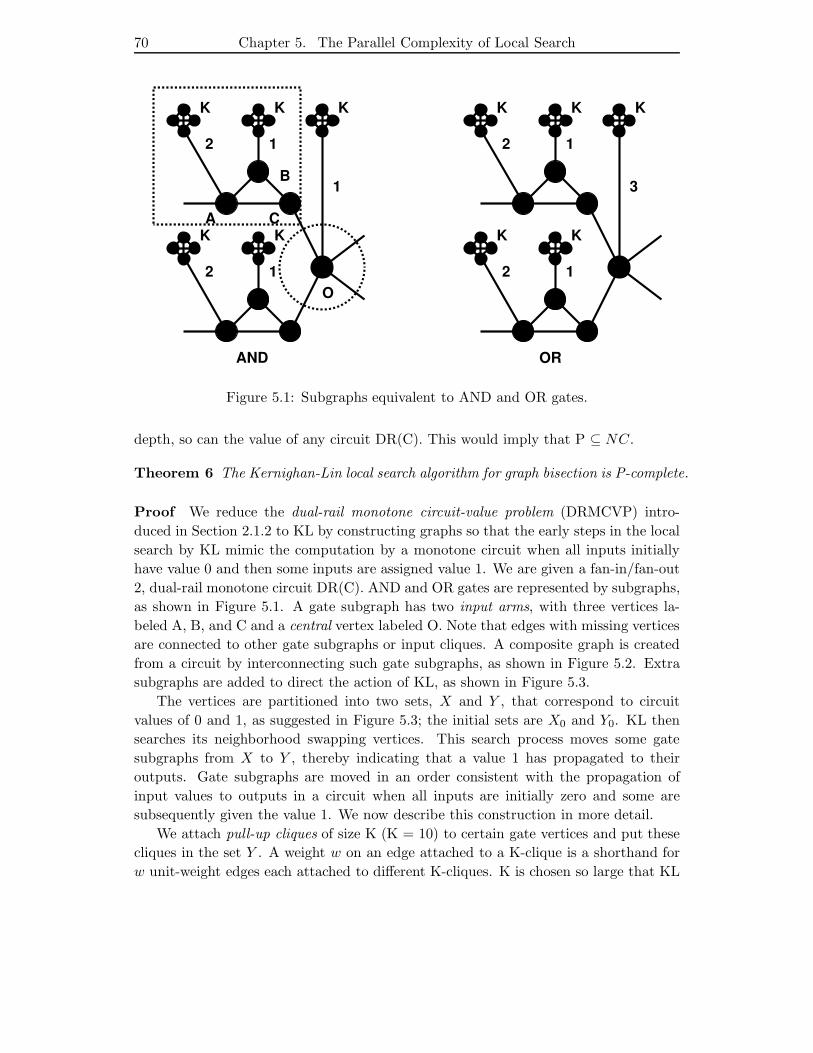
70 Chapter 5. The Parallel Complexity of Local Search
AND OR
1
K
2
K
1
K
2
K
1
K
2
K
1
K
2
KK
1
K
3
A
B
C
O
Figure 5.1: Subgraphs equivalent to AND and OR gates.
depth, so can the value of any circuit DR(C). This would imply that P ⊆ NC.
Theorem 6 The Kernighan-Lin local search algorithm for graph bisection is P-complete.
Proof We reduce the dual-rail monotone circuit-value problem (DRMCVP) intro-
duced in Section 2.1.2 to KL by constructing graphs so that the early steps in the local
search by KL mimic the computation by a monotone circuit when all inputs initially
have value 0 and then some inputs are assigned value 1. We are given a fan-in/fan-out
2, dual-rail monotone circuit DR(C). AND and OR gates are represented by subgraphs,
as shown in Figure 5.1. A gate subgraph has two input arms, with three vertices la-
beled A, B, and C and a central vertex labeled O. Note that edges with missing vertices
are connected to other gate subgraphs or input cliques. A composite graph is created
from a circuit by interconnecting such gate subgraphs, as shown in Figure 5.2. Extra
subgraphs are added to direct the action of KL, as shown in Figure 5.3.
The vertices are partitioned into two sets, X and Y , that correspond to circuit
values of 0 and 1, as suggested in Figure 5.3; the initial sets are X0 and Y0. KL then
searches its neighborhood swapping vertices. This search process moves some gate
subgraphs from X to Y , thereby indicating that a value 1 has propagated to their
outputs. Gate subgraphs are moved in an order consistent with the propagation of
input values to outputs in a circuit when all inputs are initially zero and some are
subsequently given the value 1. We now describe this construction in more detail.
We attach pull-up cliques of size K (K = 10) to certain gate vertices and put these
cliques in the set Y . A weight w on an edge attached to a K-clique is a shorthand for
w unit-weight edges each attached to different K-cliques. K is chosen so large that KL
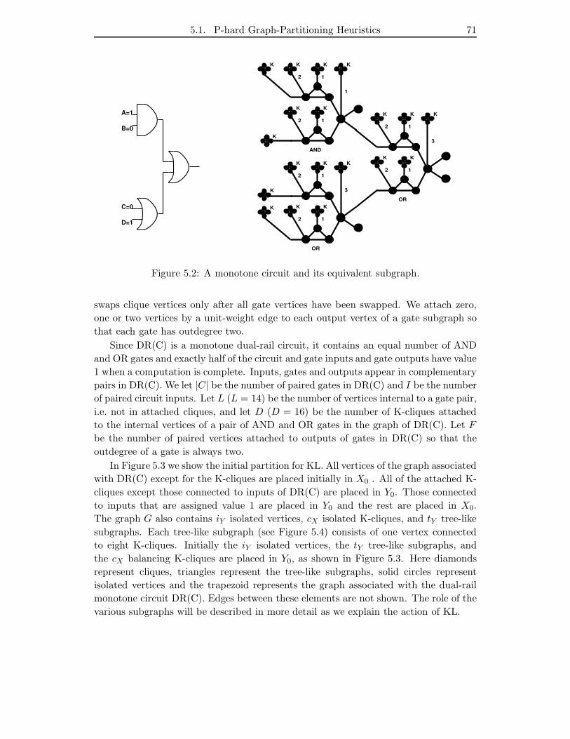
5.1. P-hard Graph-Partitioning Heuristics 71
A=1
C=0
D=1
B=0
AND
1
K
2
K
1
K
2
K K
1
OR
1
K
2
K
1
K
2
K K
3
OR
1
K
2
K
1
K
2
K K
3
K
K
K
K
Figure 5.2: A monotone circuit and its equivalent subgraph.
swaps clique vertices only after all gate vertices have been swapped. We attach zero,
one or two vertices by a unit-weight edge to each output vertex of a gate subgraph so
that each gate has outdegree two.
Since DR(C) is a monotone dual-rail circuit, it contains an equal number of AND
and OR gates and exactly half of the circuit and gate inputs and gate outputs have value
1 when a computation is complete. Inputs, gates and outputs appear in complementary
pairs in DR(C). We let |C| be the number of paired gates in DR(C) and I be the number
of paired circuit inputs. Let L (L = 14) be the number of vertices internal to a gate pair,
i.e. not in attached cliques, and let D (D = 16) be the number of K-cliques attached
to the internal vertices of a pair of AND and OR gates in the graph of DR(C). Let F
be the number of paired vertices attached to outputs of gates in DR(C) so that the
outdegree of a gate is always two.
In Figure 5.3 we show the initial partition for KL. All vertices of the graph associated
with DR(C) except for the K-cliques are placed initially in X0 . All of the attached K-
cliques except those connected to inputs of DR(C) are placed in Y0. Those connected
to inputs that are assigned value 1 are placed in Y0 and the rest are placed in X0.
The graph G also contains iY isolated vertices, cX isolated K-cliques, and tY tree-like
subgraphs. Each tree-like subgraph (see Figure 5.4) consists of one vertex connected
to eight K-cliques. Initially the iY isolated vertices, the tY tree-like subgraphs, and
the cX balancing K-cliques are placed in Y0, as shown in Figure 5.3. Here diamonds
represent cliques, triangles represent the tree-like subgraphs, solid circles represent
isolated vertices and the trapezoid represents the graph associated with the dual-rail
monotone circuit DR(C). Edges between these elements are not shown. The role of the
various subgraphs will be described in more detail as we explain the action of KL.
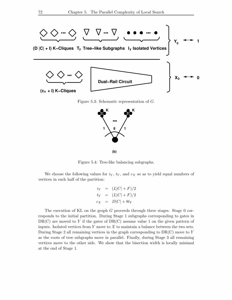
72 Chapter 5. The Parallel Complexity of Local Search
X0 0
0Y 1
Dual−Rail Circuit
(D |C| + I) K−Cliques
(c + I) K−Cliques
I Isolated VerticesT Tree−like Subgraphs
x
yy
Figure 5.3: Schematic representation of G.
K K
1 1
(b)
8
Figure 5.4: Tree-like balancing subgraphs.
We choose the following values for iY , tY , and cX so as to yield equal numbers of
vertices in each half of the partition:
iY = (L|C| + F )/2
tY = (L|C| + F )/2
cX = D|C| + 8tY
The execution of KL on the graph G proceeds through three stages. Stage 0 cor-
responds to the initial partition. During Stage 1 subgraphs corresponding to gates in
DR(C) are moved to Y if the gates of DR(C) assume value 1 on the given pattern of
inputs. Isolated vertices from Y move to X to maintain a balance between the two sets.
During Stage 2 all remaining vertices in the graph corresponding to DR(C) move to Y
as the roots of tree subgraphs move in parallel. Finally, during Stage 3 all remaining
vertices move to the other side. We show that the bisection width is locally minimal
at the end of Stage 1.

5.1. P-hard Graph-Partitioning Heuristics 73
Stage 0 We compute bw0(G), the initial bisection width of G, by using the fact that
DR(C) is a dual-rail circuit. Ignoring K-cliques attached to inputs, each gate and its
dual are connected to D K-cliques by unit-weight edges. Each of these edges contributes
one to the initial bisection width bw0(G). I edges connected to K-cliques representing
inputs of value 1 in DR(C) also contribute to bw0(G) and no other edges cross the
partition. Consequently,
bw0(G) = D|C| + I
Stage 1 As described in Section 4.3.3, KL swaps and freezes the pair of vertices on
opposite sides of the partition that causes the largest reduction (or smallest increase) in
the width of the bisection. The only vertices in X whose swapping can initially reduce
the width of the bisection are those connected to inputs whose value is 1. Moving one of
these by exchanging it with one of the iY isolated vertices in Y decreases the bisection
width by one. This may change the conditions at an adjacent vertex so that swapping
this vertex causes yet another reduction in the bisection width. Vertex swapping with
isolated vertices continues until all gates that should eventually have value 1 do have
value 1. Since DR(C) is a dual-rail circuit, at this time exactly half of the non-clique
vertices in DR(C) have been swapped with iY isolated vertices from Y . At this point
no more isolated vertices are available; any further swapping of a vertex in DR(C)∩X
causes the bisection width to increase.
At the end of Stage 1 the value of the circuit can be computed from the partition
P by determining on which side of the partition the output vertex falls. We show
later that the OR and AND gate subgraphs have been designed correctly, i.e. that gate
subgraphs mimic the operation of gates and compute the correct circuit value of every
gate.
Let us look now at the the bisection width bw1(G) of the graph at the end of Stage 1.
Consider an OR gate in DR(C) and its dual AND gate. When both inputs to the OR
gate are 0, the contribution of the gate to the bisection width is 9 while nothing is
contributed by its dual AND gate. When the inputs to both gates are 0 and 1, their
combined contribution to the bisection width is 9. When the two inputs to the OR
gate are 1, all vertices in the equivalent subgraph have moved to Y and there is no
contribution to the bisection width. The dual AND gate has both inputs 0 and the
contribution to the bisection width is 7. It follows that
bw1(G) = 9|C| − 2nOR1,1
where nOR1,1 is the number of OR gates in DR(C) that have both inputs 1.
Stage 2 The next gates in X to be moved are also from DR(C). To see this, observe
that no vertex in DR(C) has degree more than 7; one vertex cannot cause an increase
of more than 7 in the bisection width. All other vertices in X are in the K-cliques,
with K = 10, and would cause an increase of at least 9 in the bisection width. Each

74 Chapter 5. The Parallel Complexity of Local Search
vertex in DR(C) is swapped with a vertex of degree 8 in a tree-like subgraph because
this pair causes the smallest increase in the bisection width. Consequently, each swap
of a remaining vertex with one from Y causes an increase in the bisection width of at
least 1. The bisection width bw2, after all vertices have been moved, satisfies
bw2(G) = 8tY + I
since tY tree vertices of degree 8 have changed sides, I input edges in DR(C) are
connected to K-cliques in X and no other edges cross the cut.
Stage 3 The only vertices available for moving at Stage 3 are the K-cliques. A clique
is attached to at most one vertex in the rest of the graph. As a clique moves, the
bisection width first increases and then decreases, but the clique contributes positively
to the bisection width until it has changed sides completely. Thus, we can guarantee
that the bisection width during these moves never falls below bw0.
To summarize, the steps taken by KL cause the bisection width to decrease uni-
formly from bw0 to bw1, then to increase uniformly to bw2, with bw2 > bw0, and then
to decrease back to bw0. We conclude that the best partition in the KL-neighborhood
corresponds exactly to the point at which the value of DR(C) has been computed.
The gate values of DR(C) can be computed in logspace from this partition by looping
through all vertices of G, checking whether they are output vertices, and using the side
of the partition as gate value.
Operation of Gate Subgraphs We now verify the correct operation of the gate
subgraphs during Stage 1 of the KL algorithm, and demonstrate that gate subgraphs
mimic gate operations.
In the KL heuristic, vertices are frozen once they have moved. Therefore, once
the input arm vertices A, B, and C and the central vertex O have moved to X, they
are unavailable for further swaps. As we have seen, the locally minimal bisection is
assumed at the end of Stage 1. During Stage 1, we need consider only swaps of gate
vertices in X with isolated vertices in Y , and only swaps that improve the partition
are accepted. The various attached pull-up cliques do not move during Stage 1.
The gate state of a gate subgraph is the current assignment of its vertices to either
X or Y . Once the local search algorithm starts operating on the initial partition, it
changes vertex assignments by moving vertices between sets X and Y , thus causing
transitions from one gate state to another. Special gate states are the initial states,
where vertices are on the X side of the partition (with the exception of the pull-up
cliques) and the minimal states reached at the end of Stage 1, in which no more positive
gain (bisection-width improving) moves can be executed by the local search algorithm.
We show that a sequence of transitions starting from the initial state of a gate
subgraph eventually leads to a minimal state. To do this we examine all possible states
and all possible state transitions during the course of the local search algorithm.
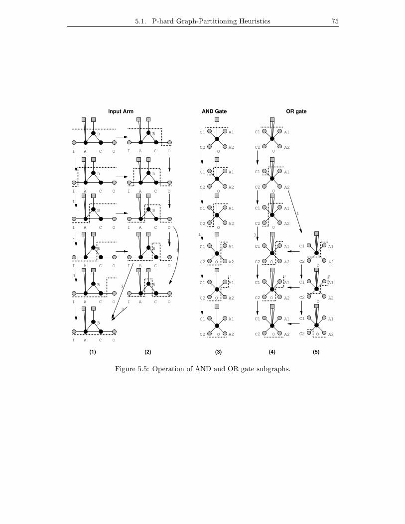
5.1. P-hard Graph-Partitioning Heuristics 75
A
B
CI O
A
B
CI O
A
B
CI O
A
B
CI O
A
B
CI O
A
B
CI O
A
B
CI O
A
B
CI O
A
B
CI O
A
B
CI O
A CI O
B
O
C1
C2
O
C1
C2
O
C1
C2
O
C1
C2
O
C1
C2
O
C1
C2
A1
A2
A1
A2
A1
A2
A1
A2
A1
A2
A1
A2
1
1
1
1
1
1
3
3
1
(1) (2) (3)
Input Arm AND Gate
O
C1
C2
O
C1
C2
O
C1
C2
O
C1
C2
O
C1
C2
O
C1
C2
A1
A2
A1
A2
A1
A2
A1
A2
A1
A2
A1
A2
O
C1
C2
O
C1
C2
O
C1
C2
A1
A2
A1
A2
A1
A2
1
3
(4) (5)
OR gate
Figure 5.5: Operation of AND and OR gate subgraphs.
76 Chapter 5. The Parallel Complexity of Local Search
For simplicity, the AND and OR gate subgraphs are decomposed. As mentioned
above, every gate has two input arms, with three vertices A, B, and C (Columns 1
and 2 in Figure 5.5.) The gate also has a central vertex labeled O (Columns 3, 4, and
5 in Figure 5.5.) Vertex C1 (C2) is the vertex C of the attached first (second) input
arm, and vertex A1 (A2) is the vertex A of the attached first (second) output arm, or
a single vertex, if the gate has less than two outputs. Depending on whether this gate
is an AND or an OR gate, either one or three edges attach the central vertex to its
pull-up cliques.
Column 1 of Figure 5.5 shows the operation of the input arm when the central
vertex is still in X, and an input I moves to Y : first vertex A, then B, and then C
move to Y , all with a gain of 1. Column 2 of Figure 5.5 handles the special case where
the input arm is connected to the central vertex O of an OR gate, whose other input
and central vertex have already moved to Y . The vertex C of the input arm stays in X
unless vertex A moves from X to Y , because all possible moves have negative gain. As
a consequence, gate subgraphs mimic the operation of gates in that a change in output
does not cause the change of an input. In Column 2 of Figure 5.5, Vertex C in the 4th
state and vertex B in the 5th state move with gain 3 to the 6th state in Column 1; all
other vertices move with gain 1. Column 3 of Figure 5.5 shows the states of the central
vertex of an AND gate. Note that only one pull-up clique is attached to it. Vertex O
moves to Y with gain 1 only when both vertices C1 and C2 have moved to Y . Note
that the isolating effect of vertex C in the input arm now assures that the vertices A1
and A2 never move before the central vertex 0 moves. Columns 4 and 5 of Figure 5.5
show the states of the central vertex of an OR gate. Vertex O moves to Y with gain 1
when either C1 or C2 have moved to Y , and moves to Y with gain 3 when both vertices
C1 and C2 have previously moved to Y .
All states but the minimal ones allow moves with positive gain. Consequently
improving swaps are executed until a minimal state is reached, and thus our gate
subgraphs operate correctly during Stage 1 of the KL local search algorithm. 2
In the Fiduccia-Mattheyses (FM) local search algorithm for graph bisection de-
scribed in Section 4.3.3, the move set is altered to let single vertices be moved to the
other side of the partition and then frozen. Note that the above reduction, and in
particular the operation of the gate subgraphs shown in Figure 5.5, remains correct in
the FM-N neighborhood. The FM balance condition, that the smaller of two sets in
a partition must have a size that is an approximate fraction r of the total number of
vertices, does not influence the operation of the gate subgraphs. Let |V | be the number
of vertices in G. We add |V |2 K-cliques on each side of the partition. It can be shown
that this construction satisfies any balance condition r.
Theorem 7 The Fiduccia-Mattheyses local search algorithm for graph bisection is P-
complete.

5.1. P-hard Graph-Partitioning Heuristics 77
5.1.2 P-Hardness of the SA Heuristic
ZT-SA, the “zero-temperature” version of graph partitioning by SA, defined in Sec-
tion 4.1.2, is a type of probabilistic steepest-descent algorithm. We first show that
ZT-SA is in the class BPP (see Section 2.1.1), so the error probability in finding a local
minimum can be made arbitrarily small. We then show that any heuristic that accepts
only swaps with positive gain is P-hard; it can solve the circuit-value problem and is
unlikely to be in NC. Instances of such heuristics are ZT-SA, deterministic swap, and
also the Mob heuristic (with mob size 1) which we introduce in Section 6.1.
Theorem 8 The ZT-SA heuristic is in BPP.
Proof In the proof of Theorem 6 in Section 5.1.1 a boolean circuit C with n gates
was transformed into a graph G with |V | = O(n) vertices and |E| = O(n) edges. The
initial bisection width of G is therefore at most |E|. Let PE be the probability that
ZT-SA does not reach a local minimum after execution of a polynomial number q(n)
of steps. We have to show that PE ≤ 1/2− ǫ, i.e. that the error probability is bounded
away from 1/2 by a constant.
ZT-SA must execute |E| moves that improve the bisection width. Divide the q(n)
time steps of the procedure into |E| intervals of m(n) = q(n)/|E| of time steps each.
If the procedure fails to find the local minimum in time q(n), then by the pigeon hole
principle at least one of these intervals does not contain a swap that improves the
bisection width. Thus, the probability PE of an unsuccessful execution is bounded
above by the probability that a pair of vertices is not swapped in one or more of these
|E| intervals.
Since at each step until the local minimum is reached there is at least one vertex
in each half of the partition which can be selected and swapped, it follows that the
conditional probability of failing to make a successful swap on any given time step,
conditioned on all prior actions, is at most 1− 4/|V |2, since there are [|V |/2]2 possible
pairs to swap. The probability of failing to find a successful swap in a set of m(n)
contiguous time steps is thus at most (1 − 4/|V |2)m(n). The probability of this event
happening in one or more of the E intervals is an upper bound to PE and satisfies the
inequality
PE ≤ |E|(1 − 4/|V |2)m(n) ≤ |E|e−4m(n)/|V |2
Thus, if we choose q(n) for some constant ǫ so that
q(n) ≥ |E|4
|V |2[(− ln(1/2 − ǫ)) + ln |E|]
then we have PE ≤ 1/2 − ǫ. Since both |V | and |E| in our constructed graph G are
proportional to n, it follows that q(n) need grow only slightly faster than n3. ZT-SA
computes with bounded error probability the correct circuit value for C. 2
78 Chapter 5. The Parallel Complexity of Local Search
Theorem 9 Let H be a graph-partitioning algorithm operating on the SWAP neigh-
borhood. If H accepts only vertex swaps that improve the bisection width whenever such
a swap is available, then H is P-hard.
Proof The SWAP neighborhood for graph partitioning was defined in Section 4.3.2.
We reduce DRMCVP to H by constructing graphs so that the steps in the local search
mimic the computation by a monotone circuit when all inputs initially have value 0
and then some inputs are assigned value 1. We are given a fan-in/fan-out 2, dual-rail
monotone circuit DR(C). The construction of the graph G and its initial partition is
exactly the same as in the KL reduction, and is in logspace and deterministic.
As in the KL reduction, we must show that a sequence of transitions starting from
the initial state of a gate subgraph eventually leads to a minimal state. Correct values
for all gates in DR(C) correspond to a local minimum that H reaches and cannot leave.
The main difference from the KL reduction is that vertices are not frozen; they can
move back and forth across the partition boundary. A vertex swap consists of a vertex
move from X to Y and a vertex move from Y to X.
We know that H accepts only positive-gain (bisection-width-improving) swaps, but
the exact rule for selecting vertices to swap is left unspecified. We show by induc-
tion that the gate subgraphs continue to operate correctly as they move. By correct
operation we mean:
(a) At all instants of time the gate states are identical to those of the KL algorithm
shown in Figure 5.5 in Section 5.1.1.
(b) Vertex moves from X to Y have gain 0, 1 or 3.
(c) Vertex moves from Y to X have gain 0 or −1.
(d) Only positive gain-swaps are accepted by H.
Initially assumptions (a) to (d) hold. We again examine in Figure 5.5 all possible
states and all possible state transitions that can occur during the execution of the local
search algorithm. Vertices belonging to the cliques and tree-like subgraphs cannot move
because they cause large negative gains, and there are no vertices to be moved with
even larger positive gains so as to cause a vertex swap to be accepted. Vertex moves
with gain 0 are due to solitary vertices and do not influence the gate subgraphs. The
gate states and transitions of a move of a vertex in DR(C) from X to Y with gain 1
or 3 are those assumed by the KL algorithm and shown in Figure 5.5. Once in one of
these states, the only vertex moves from Y to X have gain −1 and are the inverse of
moves with gain 1.
We find that no gate states and transitions than those shown in Figure 5.5 are
possible. Therefore our assumptions that gate states are identical to the gate states of
the KL algorithm, that vertex moves from X to Y have gain 0, 1 or 3, and that vertex
5.2. P-hard Graph-Embedding Heuristics 79
moves from Y to X have gain 0 or −1 continue to hold. All states but the minimal
states allow moves with positive gain, and consequently improving swaps are executed
until a minimal state is reached. Thus our gate subgraphs operate correctly until the
H algorithm reaches a local minimum. 2
Note that we have implicitly assumed in the above proof that the gain of a vertex
swap is the sum of of the vertex move gains. If the vertex moving from X to Y and
the vertex moving from Y to X are connected by an edge, the gain of the swap is the
sum of the gains minus 2. This cannot cause the acceptance of a swap that violates the
assumption of correct gate-subgraph operation. Thus the difference in how the gain of
a swap is computed has no effect on the correct operation of the subgraphs.
Let us now apply Theorem 9 to a number of heuristics operating on the SWAP
neighborhood. These heuristics can be distinguished by the rule that selects swaps. As
long as the heuristic accepts only swaps with positive gain, it is P-hard. In ZT-SA the
vertices to be selected are chosen at random. Theorem 9 also applies to heuristics in P,
where a deterministic rule, like lexicographic-first, guides the selection of swaps, and
to the Mob heuristic given in Section 6.1, when the mob size is fixed at 1 throughout
an execution of Mob.
Theorem 10 ZT-SA is P-hard. Deterministic swap is P-complete. Mob with mob
size fixed at 1 is P-hard.
The results that local search heuristics under the SWAP and FM neighborhoods
are P-complete were obtained independently by Schaffer and Yannakakis [126].
5.2 P-hard Graph-Embedding Heuristics
We now demonstrate that traditional graph-embedding heuristics for embedding graphs
into the two-dimensional grid and the hypercube are P-hard. This is done by reducing
them to P-hard problems for graph partitioning under the SWAP neighborhood and
the CROSS cost function.
The proof of Theorem 9 in Section 5.1.2 holds for any heuristic H that accepts
only vertex swaps with positive gain. H can be a deterministic heuristic such as steep-
est descent, which selects the vertex pair with the highest positive gain for swapping,
and stops if no more positive-gain swaps are possible. To make steepest descent com-
pletely deterministic, a rule is needed to arbitrate among swaps with the same gain.
Theorem 9 in Section 5.1.2 also holds for randomized heuristics H such as random-
ized steepest descent and zero-temperature simulated annealing (ZT-SA). Randomized
steepest descent has a randomized rule to select the vertex swap of highest positive
gain among swaps of equal gain. Thus the heuristic has to run on a randomized Turing
machine RT, but the probability that RT accepts or rejects its input string in poly-
nomial time is always 1. In SA the mechanism that generates swaps is randomized.
ZT-SA, the zero-temperature version of SA, accepts only swaps of positive gain. We
80 Chapter 5. The Parallel Complexity of Local Search
have shown in Section 5.1.2 that ZT-SA is in BPP so, while it is not a polynomial-time
heuristic, the probability that the RT running ZT-SA accepts or rejects its input string
in polynomial time can be made arbitrarily small.
The following lemma is very useful in the proofs below since it connects the results
showing that graph partitioning under the SWAP neighborhood is P-hard and the local
search algorithms discussed in this section.
Lemma 10 REDUCTION LEMMA. Let H be a local search algorithm for graph em-
bedding that uses the SWAP neighborhood. H is P-hard if every swap accepted by H cor-
responds to a positive-gain swap in the local search algorithm for the graph-partitioning
problem based on the SWAP neighborhood.
The proof of this lemma follows immediately from Theorem 9 in Section 5.1.2.
There are certain graph-embedding problems whose solution can be computed in NC.
For example, an n-vertex graph can be partitioned into n/2 sets under the CROSS
cost function in NC, since this corresponds to computing a maximum matching, which
has been shown to be no harder than matrix inversion by Mulmuley et al.[94]. Un-
fortunately, known randomized and deterministic algorithms for maximum matching
use matrix inversion as a subroutine, which makes these algorithms impractical for
large graphs. The local search heuristics are interesting possible alternatives for these
problems.
5.2.1 Grid Embeddings
We now consider a family of local search algorithms for the two-dimensional grid in
which the PERIMETER cost function is used. The PERIMETER cost function is an
approximation to wiring cost and is widely used in practice. It should be noted that
this cost function does not measure wire congestion in the spaces between objects but
that reduction of wire lengths reduces congestion as a secondary effect.
Theorem 11 Let H be a local search algorithm for grid embedding using the PERIME-
TER cost function and the SWAP neighborhood. Let the grid embedding be constrained
to allow only one graph vertex per network node: S : V 7→ 0..k − 1 × 0..l − 1 with
S(i) 6= S(j) when i 6= j. If H accepts only vertex swaps that improve the cost, then H
is P-hard.
Proof We give a construction to convert the graph G = (V1, E1) used in the proof
of Theorem 9 in Section 5.1.2 into the graph G′ used here. Let (X0, Y0) be the initial
partition of G. Every vertex in G has degree at most K = 9. The construction can be
done in logspace and gives an initial embedding of G′ in the grid, as shown in Figure 5.6,
in which every positive-gain swap accepted by H corresponds to a positive-gain swap in
the associated graph-partitioning problem. Thus, by the reduction lemma, H is P-hard.
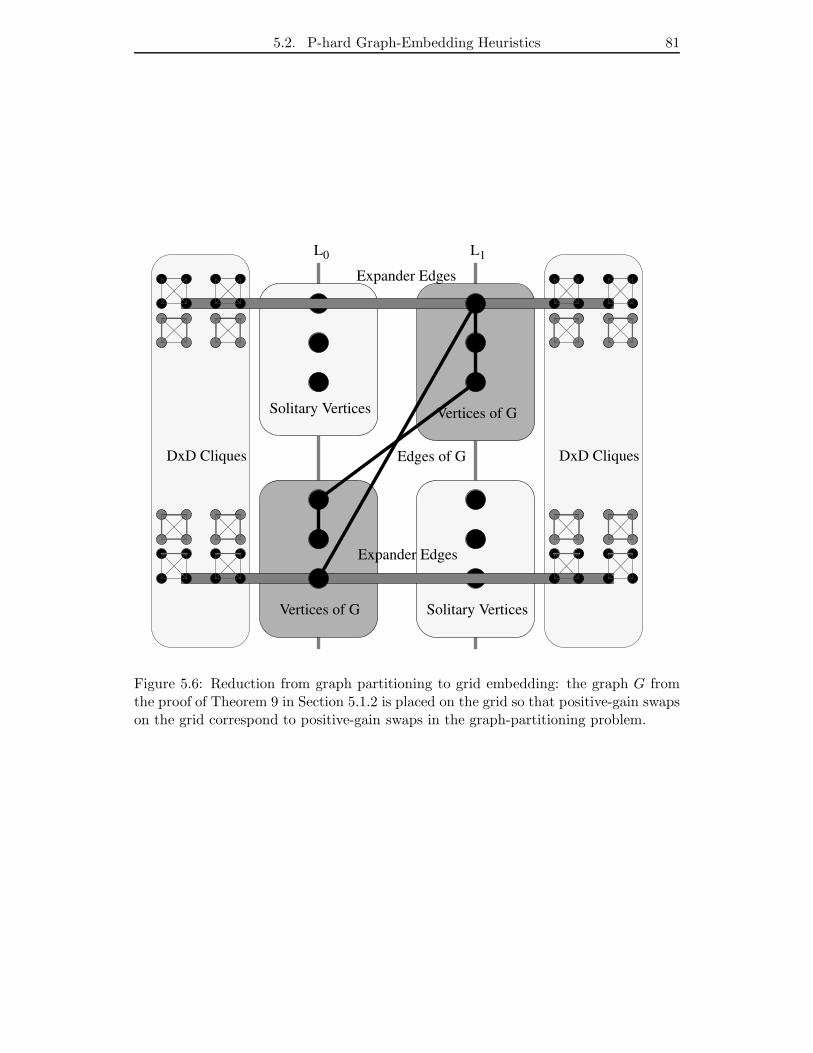
5.2. P-hard Graph-Embedding Heuristics 81
DxD Cliques
Vertices of G Solitary Vertices
Vertices of GSolitary Vertices
DxD CliquesEdges of G
Expander Edges
Expander Edges
L0 L1
Figure 5.6: Reduction from graph partitioning to grid embedding: the graph G fromthe proof of Theorem 9 in Section 5.1.2 is placed on the grid so that positive-gain swapson the grid correspond to positive-gain swaps in the graph-partitioning problem.
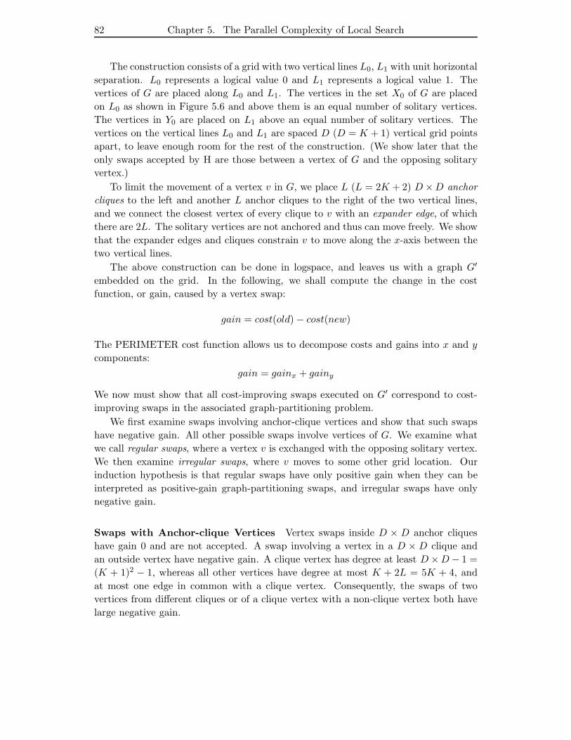
82 Chapter 5. The Parallel Complexity of Local Search
The construction consists of a grid with two vertical lines L0, L1 with unit horizontal
separation. L0 represents a logical value 0 and L1 represents a logical value 1. The
vertices of G are placed along L0 and L1. The vertices in the set X0 of G are placed
on L0 as shown in Figure 5.6 and above them is an equal number of solitary vertices.
The vertices in Y0 are placed on L1 above an equal number of solitary vertices. The
vertices on the vertical lines L0 and L1 are spaced D (D = K + 1) vertical grid points
apart, to leave enough room for the rest of the construction. (We show later that the
only swaps accepted by H are those between a vertex of G and the opposing solitary
vertex.)
To limit the movement of a vertex v in G, we place L (L = 2K + 2) D ×D anchor
cliques to the left and another L anchor cliques to the right of the two vertical lines,
and we connect the closest vertex of every clique to v with an expander edge, of which
there are 2L. The solitary vertices are not anchored and thus can move freely. We show
that the expander edges and cliques constrain v to move along the x-axis between the
two vertical lines.
The above construction can be done in logspace, and leaves us with a graph G′
embedded on the grid. In the following, we shall compute the change in the cost
function, or gain, caused by a vertex swap:
gain = cost(old) − cost(new)
The PERIMETER cost function allows us to decompose costs and gains into x and y
components:
gain = gainx + gainy
We now must show that all cost-improving swaps executed on G′ correspond to cost-
improving swaps in the associated graph-partitioning problem.
We first examine swaps involving anchor-clique vertices and show that such swaps
have negative gain. All other possible swaps involve vertices of G. We examine what
we call regular swaps, where a vertex v is exchanged with the opposing solitary vertex.
We then examine irregular swaps, where v moves to some other grid location. Our
induction hypothesis is that regular swaps have only positive gain when they can be
interpreted as positive-gain graph-partitioning swaps, and irregular swaps have only
negative gain.
Swaps with Anchor-clique Vertices Vertex swaps inside D × D anchor cliques
have gain 0 and are not accepted. A swap involving a vertex in a D × D clique and
an outside vertex have negative gain. A clique vertex has degree at least D ×D − 1 =
(K + 1)2 − 1, whereas all other vertices have degree at most K + 2L = 5K + 4, and
at most one edge in common with a clique vertex. Consequently, the swaps of two
vertices from different cliques or of a clique vertex with a non-clique vertex both have
large negative gain.
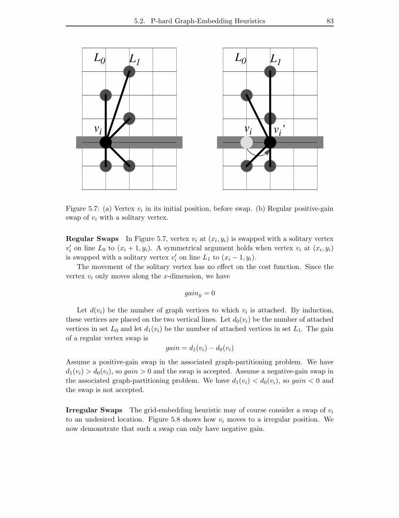
5.2. P-hard Graph-Embedding Heuristics 83
vi vi vi’
L1L0L1
L0
Figure 5.7: (a) Vertex vi in its initial position, before swap. (b) Regular positive-gainswap of vi with a solitary vertex.
Regular Swaps In Figure 5.7, vertex vi at (xi, yi) is swapped with a solitary vertex
v′i on line L0 to (xi + 1, yi). A symmetrical argument holds when vertex vi at (xi, yi)
is swapped with a solitary vertex v′i on line L1 to (xi − 1, yi).
The movement of the solitary vertex has no effect on the cost function. Since the
vertex vi only moves along the x-dimension, we have
gainy = 0
Let d(vi) be the number of graph vertices to which vi is attached. By induction,
these vertices are placed on the two vertical lines. Let d0(vi) be the number of attached
vertices in set L0 and let d1(vi) be the number of attached vertices in set L1. The gain
of a regular vertex swap is
gain = d1(vi) − d0(vi)
Assume a positive-gain swap in the associated graph-partitioning problem. We have
d1(vi) > d0(vi), so gain > 0 and the swap is accepted. Assume a negative-gain swap in
the associated graph-partitioning problem. We have d1(vi) < d0(vi), so gain < 0 and
the swap is not accepted.
Irregular Swaps The grid-embedding heuristic may of course consider a swap of vi
to an undesired location. Figure 5.8 shows how vi moves to a irregular position. We
now demonstrate that such a swap can only have negative gain.
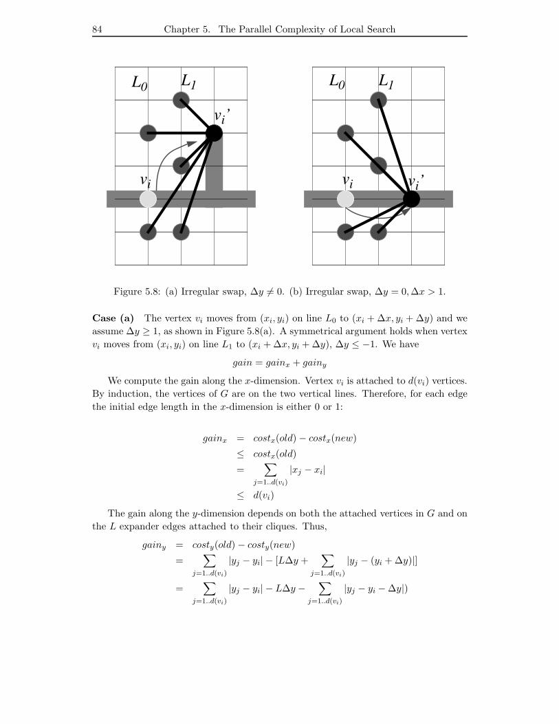
84 Chapter 5. The Parallel Complexity of Local Search
vi vi vi’
vi’
L1L0L1L0
Figure 5.8: (a) Irregular swap, ∆y 6= 0. (b) Irregular swap, ∆y = 0,∆x > 1.
Case (a) The vertex vi moves from (xi, yi) on line L0 to (xi + ∆x, yi + ∆y) and we
assume ∆y ≥ 1, as shown in Figure 5.8(a). A symmetrical argument holds when vertex
vi moves from (xi, yi) on line L1 to (xi + ∆x, yi + ∆y), ∆y ≤ −1. We have
gain = gainx + gainy
We compute the gain along the x-dimension. Vertex vi is attached to d(vi) vertices.
By induction, the vertices of G are on the two vertical lines. Therefore, for each edge
the initial edge length in the x-dimension is either 0 or 1:
gainx = costx(old) − costx(new)
≤ costx(old)
=∑
j=1..d(vi)
|xj − xi|
≤ d(vi)
The gain along the y-dimension depends on both the attached vertices in G and on
the L expander edges attached to their cliques. Thus,
gainy = costy(old) − costy(new)
=∑
j=1..d(vi)
|yj − yi| − [L∆y +∑
j=1..d(vi)
|yj − (yi + ∆y)|]
=∑
j=1..d(vi)
|yj − yi| − L∆y −∑
j=1..d(vi)
|yj − yi − ∆y|)

5.2. P-hard Graph-Embedding Heuristics 85
Since we have |a| − |b| ≤ |a − b|,
gainy ≤∑
j=1..d(vi)
|yj − yi| − L|∆y| −∑
j=1..d(vi)
|yj − yi| −∑
j=1..d(vi)
−|∆y|
= −L|∆y| + d(vi)|∆y|= (d(vi) − L)|∆y|
We assumed above that |∆y| ≥ 1. In the following, let K = maxvi∈G d(vi) be the
maximum degree of G. We shall set the parameter L so that L = 2K + 2 ≥ 2d(vi) + 2:
gain ≤ d(vi) + (d(vi) − L)|∆y|≤ (d(vi) + d(vi) − L)|∆y|< 0
Case (b) Vertex vi moves from (xi, yi) on line L0 to (xi + ∆x, yi), ∆x > 1, as shown
in Figure 5.8(b). A symmetrical argument holds for vertex moves from (xi, yi) on line
L1 to (xi − ∆x, yi), ∆x > 1.
As the vertex vi moves only along the x-dimension, we have gainy = 0. By induc-
tion, all vertices in G attached to vi are placed on the two vertical lines. Thus, before
vi moves, the length of all edges attached to vi in the x-dimension is either 0 or 1.
After vi moves to (xi + ∆x, yi), ∆x > 1, every edge that attaches vi to other vertices
in G has length of at least 1. Since every edge length remains the same or is stretched
along the x-dimension, this vertex move can only increase the cost. This move is not
accepted by H, as it does not have positive gain.
Case (c) Vertex vi moves from (xi, yi) on line L0 to (xi − ∆x, yi), ∆x > 0. A
symmetrical argument holds for vertex moves from (xi, yi) on line L1 to (xi + ∆x, yi),
∆x > 0.
As the vertex vi moves only along the x-dimension, we have gainy = 0. This vertex
move can only increase the cost, since every edge is stretched along the x-dimension.
This move is not accepted by H, as it has negative gain.
To summarize, the conditions of the reduction lemma hold for a regular swap. Other
swaps cannot be accepted by H since they have negative gain. No swaps are accepted
that violate our inductive assumption that the vertices of G are placed on the two
vertical lines. 2
5.2.2 Hypercube Embeddings
Theorem 12 Let H be a local search algorithm for hypercube embedding using the
HCUBE cost function and the SWAP neighborhood. Let the hypercube embedding be
constrained to allow only one graph vertex per network node: S : V 7→ 0..2k − 1 with

86 Chapter 5. The Parallel Complexity of Local Search
S(i) 6= S(j), i 6= j. If H accepts only vertex swaps that improve the cost, then H is
P-hard.
Proof We give a construction to convert the graph G = (V1, E1) used in the proof
of Theorem 9 in Section 5.1.2 into the graph G′ used here. Let (X0, Y0) be the initial
partition of G. Every vertex in G has degree at most K = 9. The construction can be
done in logspace and gives an initial embedding of G′ in the hypercube in which every
positive-gain swap accepted by H corresponds to a positive-gain swap in the associated
graph-partitioning problem. Thus, by the reduction lemma, H is P-hard.
To construct G′, let the tuple (a1, a2, a3, a4) represent the k-bit address of a hyper-
cube node, where the fields a1, a2, a3, a4 are binary numbers with constant k1, k2, k3, k4
number of bits, k = k1+k2+k3+k4. We can associate the individual fields a1, a2, a3, a4
with collections of hyperplanes. As a shorthand, 0 represents a binary number of arbi-
trary length in which all bits are 0.
Field a1 has length k1 = 1. Graph vertices of G and their associated solitary
vertices are placed on either side of the hyperplane a1. All addresses (0, a2, a3, a4)
denote a logical value of 0, while addresses (1, a2, a3, a4) denote a logical value of 1.
Field a2 has length k2 = ⌈log |V1|⌉, where |V1| is the number of vertices in G. If
vertex vi is in the set X0 of G, vi is placed at (0, i, 0, 0) and a solitary vertex is placed
at (1, i, 0, 0). If vertex vi is in the set X1 of G, vi is placed at (1, i, 0, 0) and a solitary
vertex is placed at (0, i, 0, 0). The solitary vertices are not anchored and thus can move
freely.
To limit the movement of a vertex vi in G, we place L (L = K + 5) anchor vertices
for every vertex vi. Field a3 with length k3 = L is used for the placement of the anchor
vertices. Let el be a binary number of length k3 in which the lth bit is 1 and all
other bits are 0. Anchor vertices are placed at addresses (0, i, e1, 0), . . ., (0, i, eL, 0) for
every vertex vi. Another set of anchor vertices is placed at addresses (1, i, e1, 0), . . .,
(1, i, eL, 0) for every vertex vi. Let E0 be the set of anchor vertices at (0, i, e1, 0), . . .,
(0, i, eL, 0) and let E1 be the set of anchor vertices at (1, i, e1, 0), . . .,(1, i, eL, 0). Since
we do not want the anchor vertex to move itself, every anchor vertex (0, i, ej , 0) is part
of a D × D clique, with (D = K + 1). We use field a4 with length k4 = ⌈log D × D⌉for the cliques and place the kth vertex of the D × D clique at (0, i, ej , k).
We connect each anchor vertex to vi with an expander edge. The purpose of ex-
pander edges is to constrain vi to move only between the planes (0, i, 0, 0) and (1, i, 0, 0).
Whether a vertex vi is at (0, i, 0, 0) or (1, i, 0, 0), it is connected by expander edges to
the set of anchor vertices at (0, i, e1, 0), . . ., (0, i, eL, 0) and to the set of anchor vertices
at (1, i, e1, 0), . . ., (1, i, eL, 0). One set of expander edges has cost L and the other set
has cost 2L. As we shall see later, the expander edges drastically add to the cost when
vi moves to some other location in the hypercube. The only swaps accepted by H are
those between a vertex of G and the opposing solitary vertex.
The above construction can be done in logspace, and leaves us with a graph G′
embedded on the hypercube. We now have to show that all cost-improving swaps
5.2. P-hard Graph-Embedding Heuristics 87
executed on G′ correspond to cost-improving swaps in the associated graph-partitioning
problem. We first examine swaps involving anchor-clique vertices and show that such
swaps have negative gain. All other possible swaps involve vertices of G. We examine
what we call regular swaps, in which a vertex v is exchanged with the opposing solitary
vertex. We then examine irregular swaps, in which v moves to some other hypercube
location. Our induction hypothesis is that regular swaps have positive gain only when
they can be interpreted as positive-gain graph-partitioning swaps, and irregular swaps
have only negative gain.
Swaps with Anchor-clique Vertices Vertex swaps inside D × D anchor cliques
have gain 0 and are not accepted. A swap involving a vertex in a D × D clique and
an outside vertex has negative gain. A clique vertex has degree at least D × D − 1 =
(K + 1)2 − 1, whereas all other vertices have degree at most K + 2L = 5K + 4, and
at most one edge in common with a clique vertex. Consequently, the swaps of two
vertices from different cliques or a clique vertex with a non-clique vertex both have
large negative gain.
Regular Swaps Assume vi moves from (0, i, 0, 0) to (1, i, 0, 0). A symmetrical argu-
ment holds when vi moves from (1, i, 0, 0) to (0, i, 0, 0).
Let d(vi) be the number of graph vertices to which vi is attached. By induction,
these vertices are placed at addresses (0, j, 0, 0) or (1, j, 0, 0), j 6= i. Let d0(vi) be the
number of attached vertices in L0, and let d1(vi) be the number of attached vertices in
L1. In a regular move, the expander edges do not contribute to the gain, since L edges
belonging to the anchor vertices at (0, i, e1, 0), . . ., (0, i, eL, 0) are stretched by 1 and L
edges belonging to the anchor vertices at (1, i, e1, 0), . . ., (1, i, eL, 0) are shortened by
1. The change in edge length is either 0 or 1:
gain = d1(vi) − d0(vi)
Assume a positive-gain swap in the associated graph-partitioning problem. We have
d1(vi) > d0(vi), so gain > 0 and the swap is accepted. Assume a negative-gain swap in
the associated graph-partitioning problem. We have d1(vi) < d0(vi), so gain < 0 and
the swap is not accepted.
Irregular Swaps The hypercube-embedding heuristic may of course consider a swap
of vi to an undesired location. We now show that such a swap can only have negative
gain, and is thus not accepted by H. Let us assume that vi moves from (0, i, 0, 0)
to v′i = (a1, a2, a3, a4): a symmetrical argument holds when vi moves from (1, i, 0, 0)
to (a1, a2, a3, a4). Let h = HCUBE(vi, v′i) be the distance that vi moves, and let
cost(expander(vi)) be the cost of the expander edges attached to vi. The gain of the
vertex swap is dependent on the attached edges of the graph G and the expander edges:
gain =∑
j=1..d(vi)
HCUBE(vi, vj) + cost(expander(vi))
88 Chapter 5. The Parallel Complexity of Local Search
−[∑
j=1..d(vi)
HCUBE(v′i, vj) + cost(expander(v′i))]
HCUBE() is a metric, so we can use the triangular inequality to get an upper bound
on the summation:
HCUBE(vi, vj) − HCUBE(v′i, vj) ≤ HCUBE(vi, v′i) = h
gain ≤ d(vi)h + cost(expander(vi)) − cost(expander(v′i))
It remains to consider the effect of the move from vi to v′i on the expander edges.
By induction, vi is at (0, i, 0, 0). Recall that the anchor vertex set E0 is located at
(0, i, e1, 0), . . . , (0, i, eL, 0) and the anchor vertex set E1 is at (1, i, e1, 0), . . . , (1, i, eL, 0).
The address (0, i, 0, 0) and anchor vertices in E0 have a Hamming distance of 1, and
(0, i, 0, 0) and anchor vertices in E1 have a Hamming distance of 2, so the cost of the
expander edges before the move is:
cost(expander(vi)) = L + 2L
Let us compute cost(expander(v′i)), the cost of the 2L expander edges that connect
v′i at (a1, a2, a3, a4) to E0 and E1. Let b1, b2, b3, b4 be the number of bits that change
in a1, a2, a3, a4, respectively. We have h = b1 + b2 + b3 + b4. We now examine how edge
costs are affected by a change of bits in the address fields.
(a1) The contribution of a1 to the cost of the 2L expander edges is L, both when
a1 = 0 and when a1 = 1.
(a2) A change of b2 bits in a2 causes a cost increase of b2 for every edge.
(a3) Consider the change of b3 bits in the third field. For every bit j that changes
in a3, exactly one pair of expander edges, namely that attached to (0, i, ej , 0)
and (1, i, ej , 0), contributes a cost of 0, whereas the 2L − 2 other expander edges
contribute a cost of 1. L − b3 bits do not change in a3. For every bit j that
does not change in a3, exactly one pair of expander edges, namely that attached
to (0, i, ej , 0) and (1, i, ej , 0), contributes a cost of 1, whereas all other expander
edges contribute a cost of 0. Therefore the contribution of a3 to the cost of the
2L expander edges is b3(2L − 2) + (L − b3)2.
(a4) A change of b4 bits in a4 causes a cost increase of b4 for every edge.
The total cost of the expander edges that join v′i to E0 and E1 is:
cost(expander(v′i)) = L + b22L + b3(2L − 2) + (L − b3)2 + b42L
= (L + 2L) + 2L(b2 + b3 + b4) − 4b3
In the following, let K = maxvi∈G d(vi) be the maximum degree of G. We set the
parameter L so that L = K + 5 > d(vi) + 3. Given the above equation, we consider
first the special case where h = 1.
5.3. P-hard Channel-Routing Heuristics 89
Case h = 1 When h = 1, we have b1 = 0, otherwise v′i would be at (1, i, 0, 0), a
regular position. We have b2 + b3 + b4 = 1 and b3 ≤ 1.
cost(expander(v′i)) ≥ (L + 2L) + 2L − 4
and so
gain ≤ d(vi) − 2L + 4
Since L > d(vi) + 5, we have gain < 0
Case h > 1 When h > 1, we have b2 + b3 + b4 ≥ h − 1 and b3 ≤ h.
cost(expander(v′i)) ≥ (L + 2L) + 2L(h − 1) − 4h
and so
gain ≤ d(vi)h − 2L(h − 1) + 4h
≤ d(vi)h − Lh + 4h
≤ (d(vi) + 4)h − Lh
Since L > d(vi) + 5, we have gain < 0.
To summarize, the conditions of the reduction lemma hold for a regular swap. Other
swaps cannot be accepted by H since they have negative gain. 2
5.3 P-hard Channel-Routing Heuristics
We have shown in Section 3.1 that the left-edge channel-routing algorithm can be par-
allelized to run in NC1(n), but it does not deal with column conflicts. It is therefore
tempting to design a parallel heuristic based on local search that minimizes column
conflicts or tries to remove them altogether. Brouwer and Banerjee[19] applied paral-
lel simulated annealing to the channel-routing problem and report that this approach
yields routings of high quality. The local search channel-routing problem to reduce col-
umn conflicts was defined in Section 4.5. To cast the problem of minimizing the column
conflicts of a channel routing as a local search problem, we introduced in Section 4.5 the
COLUMNS cost function and a method for making changes to one channel-routing so-
lution; this generates the SUBTRACK-SWAP neighborhood structure. In this section
we demonstrate that finding a locally minimum channel routing using the COLUMNS
cost function and the SUBTRACK-SWAP neighborhood is P-hard.
5.3.1 P-hardness of the Column-Swap Heuristic
Theorem 13 Let H be a local search algorithm for channel routing using the COLUMNS
cost function and the SUBTRACK-SWAP neighborhood. If H accepts only swaps that
improve the cost, then H is P-hard.
90 Chapter 5. The Parallel Complexity of Local Search
Proof Our proof consists of a logspace procedure to translate a given fan-in/fan-out
2 ordered monotone circuit OM(C) (see Section 2.1.2) with n gates into an initial solu-
tion R0 of a channel-routing problem. When we apply heuristic H to R0, it executes a
polynomial number q(n) of swaps and returns a solution Rq(n) that has a locally mini-
mum number of column conflicts. Rq(n) uniquely determines the value of OM(C), and
the actual value of the circuit OM(C) can then be determined from Rq(n) in logarithmic
space. Thus H is P-hard. If H is a deterministic algorithm with running time bounded
by a polynomial q(n), then H is P-complete. If the partition Rq(n) could be computed
by a deterministic circuit of polynomial size and polylogarithmic depth, so could the
value of any circuit OM(C). This would imply that P ⊆ NC.
Construction of Circuit OM(C) We show how to build the circuit elements of
OM(C) out of nets, and show how the components are placed in the channel. The
construction yields a dense channel-routing solution R0. We demonstrate that the
gates compute the correct logical values for their inputs, and that the whole circuit
construction computes the correct logical value of OM(C).
From the construction of OM(C) we can assume that the boolean value of the circuit
inputs is given as part of the problem description and that every circuit input is used
exactly once. Let the number of circuit elements in OM(C) be n. We can assume that
OM(C) is non-cyclic, and that OM(C) is ordered: all circuit elements (AND/OR gates
and input variables) are indexed so that when circuit element k depends on circuit
element i, then k > i. For every gate Gr in the circuit OM(C) we use two connecting
output wires Wk and Wl. The wires serve to propagate output values to other gates
and to buffer the gates, as will become clear later.
In the following, the weight w of a column, indicated by the number above the
columns and also illustrated by the width of the columns, is a shorthand for the w
wires attached to pins at the channel sides. Two columns of weight w overlapping
vertically cause w column conflicts.
Figure 5.9 shows the overall construction of R0 from OM(C). AND/OR gates,
circuit inputs, and connecting wires each have a pair of center subtracks, the horizontal
segments of a net that can be swapped. When the subtrack pairs remain in their initial
positions, the associated logical value of the component is 0; when the subtrack pair is
swapped, the associated logical value of the component is 1. Shown in Figure 5.9 are
the center subtracks of an input Ia, a gate Gr and two connecting output wire Wk and
Wl. The positions of two other gates Gs, Gt are sketched. To simplify Figure 5.9, the
vertical segments of the circuit elements that cause column conflicts are not shown.
We now describe how to construct the components of the circuit OM(C), which are
circuit inputs, AND/OR gates, and connecting wires, and then show how the circuit is
assembled.
Construction of Circuit Inputs Figure 5.10 shows how circuit inputs are built
out of nets. Circuit input Ia consists of one subtrack pair, the center subtrack pair
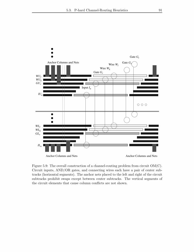
5.3. P-hard Channel-Routing Heuristics 91
GLr
WLk
WLl
Anchor Columns and Nets
Anchor Columns and Nets Anchor Columns and Nets
Gate Gr
Wire Wk
Wire Wl
Gate Gs
Gate Gt
ILa
GUr
WUk
WUl
IUa
Input Ia
Figure 5.9: The overall construction of a channel-routing problem from circuit OM(C).Circuit inputs, AND/OR gates, and connecting wires each have a pair of center sub-tracks (horizontal segments). The anchor nets placed to the left and right of the circuitsubtracks prohibit swaps except between center subtracks. The vertical segments ofthe circuit elements that cause column conflicts are not shown.

92 Chapter 5. The Parallel Complexity of Local Search
L 2
C Out
IUa
GUs
ILa
GLs
L 2
C Out
IUa
GUs
ILa
GLs
Figure 5.10: Circuit input Ia. (a) Ia = 0. (b) Ia = 1.
ILa, IUa. To demonstrate how circuit inputs are attached to gates, Figure 5.10 also
shows the subtrack pairs GLs, GUs of the gate Gs.
The problem description of the circuit OM(C) gives the boolean values of the circuit
inputs and specifies that every circuit input is used exactly once. When input Ia = 0,
one column of weight 2 is attached from the top of the channel to ILa. When Ia = 1,
one column of weight 2 is attached from the top of the channel to IUa. (The black-
bordered column of weight 2 is part of gate Gs, and is included in Figure 5.10 to show
how the circuit is assembled.)
The columns attached to the center subtrack pair ILa, IUa have weight L = x; this
weight is made so large that swapping of subtrack pair ILa, IUa causes a negative gain
that is greater than the sum of the weights on all AND/OR gates and connecting wires
in the routing of OM(C).
Construction of AND/OR Gates Figure 5.11 shows how AND and OR gates
are built out of nets. Both AND and OR gates Gr contain the center subtrack pair
GLr, GUr. Figure 5.11 also shows the two subtrack pairs WLi,WUi, WLj,WUj of the
wires Wi and Wj, which serve as inputs to gate Gr, and the subtrack pairs WLk,WUk,
WLl,WUl of the wires Wk and Wl, which are the two copies of the output of gate Gr.
The connecting wires shown in Figure 5.11 serve as buffers between gates.
The difference between AND and OR gates is that the two vertical columns attached
to the center subtrack pair GLr, GUr have weight 1 for the OR gate and weight 3 for
the AND gate. As shown, both gates have two columns of weight 2, attached from the

5.3. P-hard Channel-Routing Heuristics 93
In1 C Out1 Out2In2
81 82 2
In1 C Out1 Out2In2
83 82 2
GUr
WUj
WUk
WUl
WUi
GLr
WLj
WLk
WLl
WLi
GUr
WUj
WUk
WUl
WUi
GLr
WLj
WLk
WLl
WLi
Figure 5.11: (a) OR gate Gr. (b) AND gate Gr.
bottom of the channel to GUr, one for each input. Two columns of weight 8 attached
from the top of the channel to GLr, one for each output. The black-bordered columns
of weight 2 attach to the center subtracks WLi,WLj of wires Wi and Wj. The black-
bordered columns of weight 8 attach to the center subtracks WLk,WLl of wires Wk
and Wl.
Construction of Wires The wires propagate output values to other gates. Fig-
ure 5.12 shows how the wire is built out of nets. The wire Wk consists of one subtrack
pair, the center subtrack pair WLk,WUk. Figure 5.12 also shows the subtrack pair
GLr, GUr of the gate Gr and the subtrack pair GLs, GUs of the gate Gs.
The columns attached to the center subtrack pair WLk,WUk have weight 4. The
wire has one input column of weight 8 attached to WUk and one output column of
weight 2 attached to WLk. The black-bordered columns belong to attached gates.
Note that gate Gs must be located on center tracks that lie above the tracks assigned
to Gr and Wk. Here we need the property that OM(C) is ordered: when circuit element
k depends on circuit element i, then k > i.
Anchor Nets In Figure 5.9 the subtrack pairs ILa and IUa, GLr and GUr, WLk
and WUk and WLl and WUl can be swapped. It is highly undesirable in the operation
of our reduction to allow any other swaps of subtracks or whole tracks, and thus anchor
nets are placed to the left and right of each circuit net. As can be seen in Figure 5.9,
swapping net ILa with net GUr would result in an horizontal overlap of nets.
To prohibit the swapping of anchor nets, we attach columns of weight L to each pair
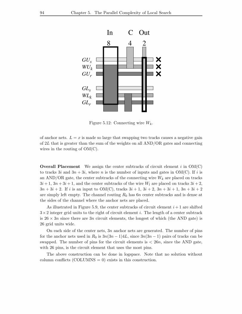
94 Chapter 5. The Parallel Complexity of Local Search
8 4 2
In C Out
GUr
WUk
GUs
GLr
WLk
GLs
Figure 5.12: Connecting wire Wk.
of anchor nets. L = x is made so large that swapping two tracks causes a negative gain
of 2L that is greater than the sum of the weights on all AND/OR gates and connecting
wires in the routing of OM(C).
Overall Placement We assign the center subtracks of circuit element i in OM(C)
to tracks 3i and 3n + 3i, where n is the number of inputs and gates in OM(C). If i is
an AND/OR gate, the center subtracks of the connecting wire Wk are placed on tracks
3i + 1, 3n + 3i + 1, and the center subtracks of the wire Wl are placed on tracks 3i + 2,
3n + 3i + 2. If i is an input to OM(C), tracks 3i + 1, 3i + 2, 3n + 3i + 1, 3n + 3i + 2
are simply left empty. The channel routing R0 has 6n center subtracks and is dense at
the sides of the channel where the anchor nets are placed.
As illustrated in Figure 5.9, the center subtracks of circuit element i+ 1 are shifted
3×2 integer grid units to the right of circuit element i. The length of a center subtrack
is 26 × 3n since there are 3n circuit elements, the longest of which (the AND gate) is
26 grid units wide.
On each side of the center nets, 3n anchor nets are generated. The number of pins
for the anchor nets used in R0 is 3n(3n− 1)4L, since 3n(3n− 1) pairs of tracks can be
swapped. The number of pins for the circuit elements is < 26n, since the AND gate,
with 26 pins, is the circuit element that uses the most pins.
The above construction can be done in logspace. Note that no solution without
column conflicts (COLUMNS = 0) exists in this construction.
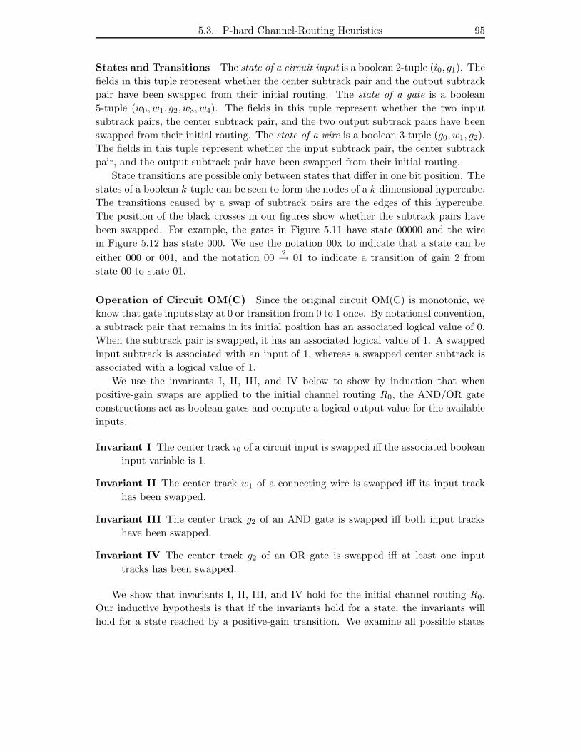
5.3. P-hard Channel-Routing Heuristics 95
States and Transitions The state of a circuit input is a boolean 2-tuple (i0, g1). The
fields in this tuple represent whether the center subtrack pair and the output subtrack
pair have been swapped from their initial routing. The state of a gate is a boolean
5-tuple (w0, w1, g2, w3, w4). The fields in this tuple represent whether the two input
subtrack pairs, the center subtrack pair, and the two output subtrack pairs have been
swapped from their initial routing. The state of a wire is a boolean 3-tuple (g0, w1, g2).
The fields in this tuple represent whether the input subtrack pair, the center subtrack
pair, and the output subtrack pair have been swapped from their initial routing.
State transitions are possible only between states that differ in one bit position. The
states of a boolean k-tuple can be seen to form the nodes of a k-dimensional hypercube.
The transitions caused by a swap of subtrack pairs are the edges of this hypercube.
The position of the black crosses in our figures show whether the subtrack pairs have
been swapped. For example, the gates in Figure 5.11 have state 00000 and the wire
in Figure 5.12 has state 000. We use the notation 00x to indicate that a state can be
either 000 or 001, and the notation 002→ 01 to indicate a transition of gain 2 from
state 00 to state 01.
Operation of Circuit OM(C) Since the original circuit OM(C) is monotonic, we
know that gate inputs stay at 0 or transition from 0 to 1 once. By notational convention,
a subtrack pair that remains in its initial position has an associated logical value of 0.
When the subtrack pair is swapped, it has an associated logical value of 1. A swapped
input subtrack is associated with an input of 1, whereas a swapped center subtrack is
associated with a logical value of 1.
We use the invariants I, II, III, and IV below to show by induction that when
positive-gain swaps are applied to the initial channel routing R0, the AND/OR gate
constructions act as boolean gates and compute a logical output value for the available
inputs.
Invariant I The center track i0 of a circuit input is swapped iff the associated boolean
input variable is 1.
Invariant II The center track w1 of a connecting wire is swapped iff its input track
has been swapped.
Invariant III The center track g2 of an AND gate is swapped iff both input tracks
have been swapped.
Invariant IV The center track g2 of an OR gate is swapped iff at least one input
tracks has been swapped.
We show that invariants I, II, III, and IV hold for the initial channel routing R0.
Our inductive hypothesis is that if the invariants hold for a state, the invariants will
hold for a state reached by a positive-gain transition. We examine all possible states
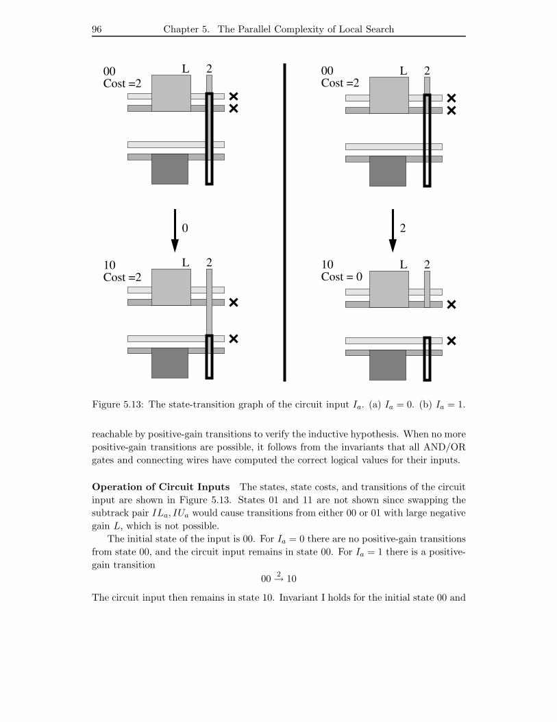
96 Chapter 5. The Parallel Complexity of Local Search
L 2 L 200Cost =2
00Cost =2
L 210Cost =2
L 210Cost = 0
0 2
Figure 5.13: The state-transition graph of the circuit input Ia. (a) Ia = 0. (b) Ia = 1.
reachable by positive-gain transitions to verify the inductive hypothesis. When no more
positive-gain transitions are possible, it follows from the invariants that all AND/OR
gates and connecting wires have computed the correct logical values for their inputs.
Operation of Circuit Inputs The states, state costs, and transitions of the circuit
input are shown in Figure 5.13. States 01 and 11 are not shown since swapping the
subtrack pair ILa, IUa would cause transitions from either 00 or 01 with large negative
gain L, which is not possible.
The initial state of the input is 00. For Ia = 0 there are no positive-gain transitions
from state 00, and the circuit input remains in state 00. For Ia = 1 there is a positive-
gain transition
002→ 10
The circuit input then remains in state 10. Invariant I holds for the initial state 00 and
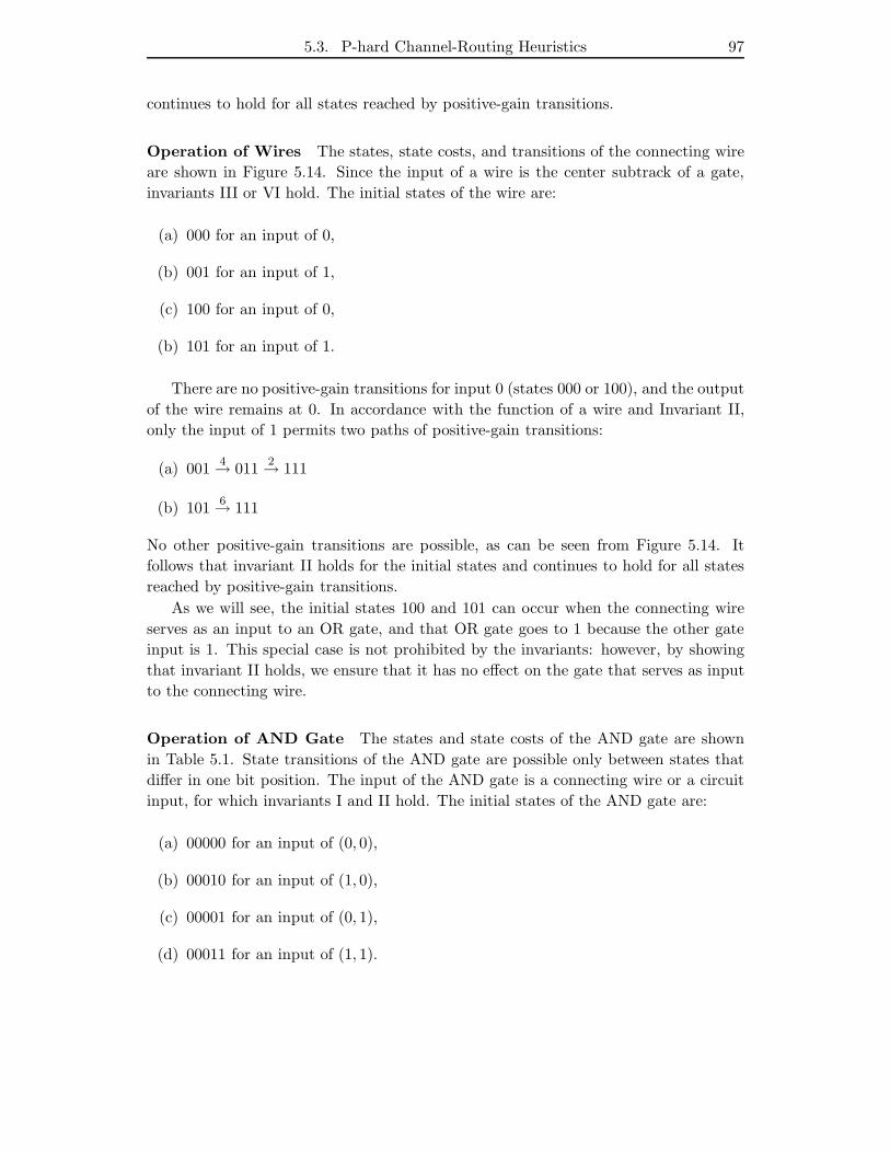
5.3. P-hard Channel-Routing Heuristics 97
continues to hold for all states reached by positive-gain transitions.
Operation of Wires The states, state costs, and transitions of the connecting wire
are shown in Figure 5.14. Since the input of a wire is the center subtrack of a gate,
invariants III or VI hold. The initial states of the wire are:
(a) 000 for an input of 0,
(b) 001 for an input of 1,
(c) 100 for an input of 0,
(b) 101 for an input of 1.
There are no positive-gain transitions for input 0 (states 000 or 100), and the output
of the wire remains at 0. In accordance with the function of a wire and Invariant II,
only the input of 1 permits two paths of positive-gain transitions:
(a) 0014→ 011
2→ 111
(b) 1016→ 111
No other positive-gain transitions are possible, as can be seen from Figure 5.14. It
follows that invariant II holds for the initial states and continues to hold for all states
reached by positive-gain transitions.
As we will see, the initial states 100 and 101 can occur when the connecting wire
serves as an input to an OR gate, and that OR gate goes to 1 because the other gate
input is 1. This special case is not prohibited by the invariants: however, by showing
that invariant II holds, we ensure that it has no effect on the gate that serves as input
to the connecting wire.
Operation of AND Gate The states and state costs of the AND gate are shown
in Table 5.1. State transitions of the AND gate are possible only between states that
differ in one bit position. The input of the AND gate is a connecting wire or a circuit
input, for which invariants I and II hold. The initial states of the AND gate are:
(a) 00000 for an input of (0, 0),
(b) 00010 for an input of (1, 0),
(c) 00001 for an input of (0, 1),
(d) 00011 for an input of (1, 1).
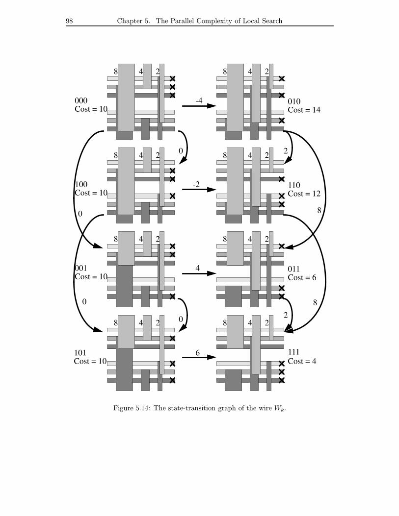
98 Chapter 5. The Parallel Complexity of Local Search
8 4 28 4 2
8 4 2 8 4 2
8 4 2
8 4 28 4 2
8 4 2
000 010
100
001
101
110
011
111
Cost = 14Cost = 10
Cost = 10
Cost = 10
Cost = 10
Cost = 12
Cost = 6
Cost = 4
-4
-2
6
4
0
0
2
2
0
0
8
8
Figure 5.14: The state-transition graph of the wire Wk.
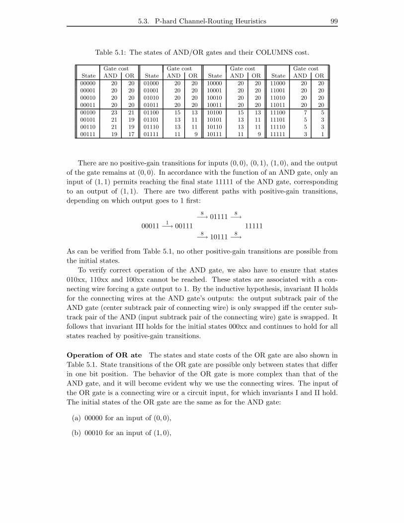
5.3. P-hard Channel-Routing Heuristics 99
Table 5.1: The states of AND/OR gates and their COLUMNS cost.
Gate cost Gate cost Gate cost Gate costState AND OR State AND OR State AND OR State AND OR
00000 20 20 01000 20 20 10000 20 20 11000 20 2000001 20 20 01001 20 20 10001 20 20 11001 20 2000010 20 20 01010 20 20 10010 20 20 11010 20 2000011 20 20 01011 20 20 10011 20 20 11011 20 20
00100 23 21 01100 15 13 10100 15 13 11100 7 500101 21 19 01101 13 11 10101 13 11 11101 5 300110 21 19 01110 13 11 10110 13 11 11110 5 300111 19 17 01111 11 9 10111 11 9 11111 3 1
There are no positive-gain transitions for inputs (0, 0), (0, 1), (1, 0), and the output
of the gate remains at (0, 0). In accordance with the function of an AND gate, only an
input of (1, 1) permits reaching the final state 11111 of the AND gate, corresponding
to an output of (1, 1). There are two different paths with positive-gain transitions,
depending on which output goes to 1 first:
000111−→ 00111
8−→ 011118−→
8−→ 101118−→
11111
As can be verified from Table 5.1, no other positive-gain transitions are possible from
the initial states.
To verify correct operation of the AND gate, we also have to ensure that states
010xx, 110xx and 100xx cannot be reached. These states are associated with a con-
necting wire forcing a gate output to 1. By the inductive hypothesis, invariant II holds
for the connecting wires at the AND gate’s outputs: the output subtrack pair of the
AND gate (center subtrack pair of connecting wire) is only swapped iff the center sub-
track pair of the AND (input subtrack pair of the connecting wire) gate is swapped. It
follows that invariant III holds for the initial states 000xx and continues to hold for all
states reached by positive-gain transitions.
Operation of OR ate The states and state costs of the OR gate are also shown in
Table 5.1. State transitions of the OR gate are possible only between states that differ
in one bit position. The behavior of the OR gate is more complex than that of the
AND gate, and it will become evident why we use the connecting wires. The input of
the OR gate is a connecting wire or a circuit input, for which invariants I and II hold.
The initial states of the OR gate are the same as for the AND gate:
(a) 00000 for an input of (0, 0),
(b) 00010 for an input of (1, 0),
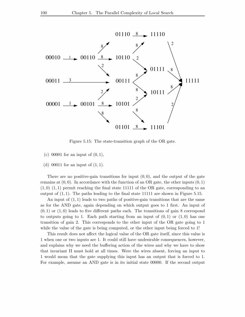
100 Chapter 5. The Parallel Complexity of Local Search
00001
00011
00101
00111
11101
10101
01101
3
1 8
8
8
2
2
8 2
8
8
00010 00110 10110
01110
1
11111
2
8
11110
01111
10111
8
8
8
8
8
2
2
Figure 5.15: The state-transition graph of the OR gate.
(c) 00001 for an input of (0, 1),
(d) 00011 for an input of (1, 1).
There are no positive-gain transitions for input (0, 0), and the output of the gate
remains at (0, 0). In accordance with the function of an OR gate, the other inputs (0, 1)
(1, 0) (1, 1) permit reaching the final state 11111 of the OR gate, corresponding to an
output of (1, 1). The paths leading to the final state 11111 are shown in Figure 5.15.
An input of (1, 1) leads to two paths of positive-gain transitions that are the same
as for the AND gate, again depending on which output goes to 1 first. An input of
(0, 1) or (1, 0) leads to five different paths each. The transitions of gain 8 correspond
to outputs going to 1. Each path starting from an input of (0, 1) or (1, 0) has one
transition of gain 2. This corresponds to the other input of the OR gate going to 1
while the value of the gate is being computed, or the other input being forced to 1!
This result does not affect the logical value of the OR gate itself, since this value is
1 when one or two inputs are 1. It could still have undesirable consequences, however,
and explains why we need the buffering action of the wires and why we have to show
that invariant II must hold at all times. Were the wires absent, forcing an input to
1 would mean that the gate supplying this input has an output that is forced to 1.
For example, assume an AND gate is in its initial state 00000. If the second output
5.3. P-hard Channel-Routing Heuristics 101
were to go to logical value 1, the AND gate would go to state 10000, a state that the
AND gate is never supposed to reach. From state 10000 there is a path of positive-gain
transitions to state 11111. Thus the output value of the AND gate would be 1, even
though both its inputs are 0.
As can be verified from Table 5.1, no positive-gain transitions other than those
shown in Figure 5.15 are possible from the initial states. To verify correct operation
of the OR gate, we also have to ensure that states 010xx, 110xx and 100xx cannot
be reached. These states are associated with a connecting wire forcing a gate output
to 1. By the inductive hypothesis, invariant II holds for the connecting wires at the
OR gate’s outputs: the output subtrack pair of the OR gate (center subtrack pair of
connecting wire) is only swapped iff the center subtrack pair of the OR (input subtrack
pair of the connecting wire) gate is swapped. It follows that invariant III holds for
the initial states 000xx and continues to hold for all states reached by positive-gain
transitions.
In summary, we have shown that all circuit elements function as required by in-
variants I, II, III, and IV. Therefore the AND/OR gate constructions obtained by the
logspace reduction from OM(C) behave as boolean gates and compute a logical output
value for the available inputs, thus computing the circuit value for OM(C). 2
5.3.2 P-hardness of the Restricted Column-Swap Heuristic
As discussed in Section 4.5.1, in the actual implementation of the local search heuristic
it is desirable to restrict the SUBTRACK-SWAP neighborhood. In the unrestricted
SUBTRACK-SWAP neighborhood, O(n2) neighbors of a channel-routing solution R
can be reached by swaps. Computing the gain ∆f for all of these swaps would waste
computational resources. In the restricted SUBTRACK-SWAP neighborhood, the as-
signed tracks are interpreted as a linear array and subtrack swaps are allowed only for
track pairs with a separation of d = ±1, 2, 4, 8, 16, . . . tracks. (See definition 27 in Sec-
tion 6.3 for a definition of separation d.) The size of the neighborhood of a solution R
is now O(n), which is a good compromise between efficiency and convergence behavior
for a local search algorithm. The proof in Section 5.3 can be extended to show that
the P-hardness result holds for the restricted SUBTRACK-SWAP neighborhood.
Corollary 4 Let H be a local search algorithm for channel routing using the COLUMNS
cost function and the SUBTRACK-SWAP neighborhood restricted to linear array swaps
with a separation d of ±1, 2, 4, 8, 16, . . . tracks. If H accepts only swaps that improve
the cost, then H is P-hard.
Proof The construction of Theorem 13 generates 3n track pairs. We simply add m
anchor nets in their own tracks above the 3n track pairs, with m = 2k − 3n, 2k−1 <
3n < 2k. The center subtracks of the circuit components in OM(C) are then d = 2k−1
apart, and are still available for swapping. 2

103
Chapter 6
The Mob Heuristic
6.1 The General Mob Heuristic
We have developed a new massively parallel heuristic, the Mob heuristic, that is closely
related to both Kernighan-Lin and simulated annealing. Our algorithm uses a mob-
selection rule to swap large sets, called mobs, of elements. The mob-selection rule
searches for an approximation to the subset that causes the largest improvement in the
embedding cost, and is designed to be computed very quickly in parallel.
We now explicitly define the Mob local search algorithm. The algorithm searches
a mob neighborhood of a solution with a given mob size. If the new solution found
has a smaller cost, the search is repeated on the neighborhood of the new solution
with the same mob size. If the cost increases, the neighborhood of the new solution
is searched with the next scheduled mob size, which is usually smaller. We assume
that Mob executes a number of steps that does not exceed q(n), a polynomial in the
number n of vertices. The probabilistic nature of Mob is reflected by sets R1, R2 of q(n)
random index variables chosen uniformly and independently from the interval (0, 1). A
schedule determines the value of the variable mob.
Our heuristic is outlined in pseudocode in Figure 6.1. Here, the neighborhood
structure MOB-NR(S,m) depends on the problem that is to be solved. We define
neighborhoods for graph partitioning and graph embedding in Section 6.2 and 6.3. A
schedule MS of mob sizes is used to control the searches.
Definition 23 A mob schedule MS of length L is a sequence [MS1,MS2, . . . ,MSL]
of integers from the interval [1, . . . , n/2].
In the following, we describe the Mob graph-partitioning algorithm and the Mob
hypercube- and grid-embedding algorithms, and report how these algorithms performed
on the CM-2. We complete the definition of the Mob heuristic by explicitly giving
the neighborhood structure MOB-NR(S,m) and the schedule MS for the particular
problem. We also describe how Mob was implemented on the CM-2. The details of the
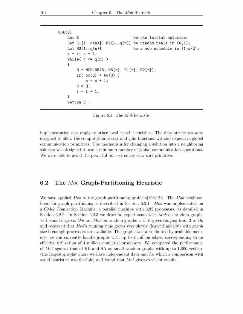
104 Chapter 6. The Mob Heuristic
Mob(S)
Let S be the initial solution;
Let R1[1..q(n)], R2[1..q(n)] be random reals in (0,1);
Let MS[1..q(n)] be a mob schedule in [1,n/2];
t = 1; s = 1;
while( t <= q(n) )
Q = MOB-NR(S, MS[s], R1[t], R2[t]);
if( bw(Q) > bw(S) )
s = s + 1;
S = Q;
t = t + 1;
return S ;
Figure 6.1: The Mob heuristic
implementation also apply to other local search heuristics. The data structures were
designed to allow the computation of cost and gain functions without expensive global
communication primitives. The mechanism for changing a solution into a neighboring
solution was designed to use a minimum number of global communication operations.
We were able to avoid the powerful but extremely slow sort primitive.
6.2 The Mob Graph-Partitioning Heuristic
We have applied Mob to the graph-partitioning problem[120,121]. The Mob neighbor-
hood for graph partitioning is described in Section 6.2.1. Mob was implemented on
a CM-2 Connection Machine, a parallel machine with 32K processors, as detailed in
Section 6.2.2. In Section 6.2.3 we describe experiments with Mob on random graphs
with small degrees. We ran Mob on random graphs with degrees ranging from 3 to 16,
and observed that Mob’s running time grows very slowly (logarithmically) with graph
size if enough processors are available. The graph sizes were limited by available mem-
ory; we can currently handle graphs with up to 2 million edges, corresponding to an
effective utilization of 4 million simulated processors. We compared the performance
of Mob against that of KL and SA on small random graphs with up to 1,000 vertices
(the largest graphs where we have independent data and for which a comparison with
serial heuristics was feasible) and found that Mob gives excellent results.
6.2. The Mob Graph-Partitioning Heuristic 105
6.2.1 The Mob Neighborhood for Graph Partitioning
Definition 24 The mob neighborhood Mob-N(P0,m) of a partition P0 = (X0, Y0) is
the set of partitions obtained from P0 by swapping a mob of m vertices from X0 with
an equal number of vertices from Y0.
The number of partitions in the neighborhood Mob-N(P,m) is
(
|V |/2m
)2
. A mob is
selected from the vertices in each set whose exchange would cause the largest individual
change in the bisection width. The rule MOB-R(P,m, r1, r2) is used to select a partition
from Mob-N(P,m):
Definition 25 The rule MOB-R(P,m, r1, r2) selects a mob of size m from Mob-N(P,m)
as follows: let r1, r2 be random real numbers drawn uniformly from the interval (0, 1).
For each vertex v, let gain(v) be the change in the bisection width if v alone changes
sides, and let gain(v) be positive if the bisection width decreases. Let SX(g) = v ∈X | gain(v) ≥ g. Choose gX such that |SX(gX + 1)| < m ≤ |SX(gX)|. Let
mp = |SX(gX)| be the size of the pre-mob SX(gX ). Each element in SX(gX ) is
indexed from 0 to mp − 1. A mob of size m is selected from SX(gX ) by adding ⌊r1mp⌋to each index modulo mp and selecting those with index less than m. A mob is selected
from Y using the same rule and the random variable r2.
The procedure is applied to both sides of the partition. The mob-selection rule,
designed to be computed very quickly in parallel, looks for a rough approximation to
the subset that causes the largest improvement in the bisection width. We implemented
routines to choose exactly m vertices whose individual gains are largest, but neither
sorting or randomized methods provided adequate performance. Instead, we choose
vertices at random among all vertices in SX(gX). While in so doing we may miss some
vertices with large gain, our heuristic is very effective.
Our heuristic starts with an initial random partition of the vertices of a graph. As
explained above, it then forms a pre-mob of vertices from each set of the partition on
the basis of the effect of individual vertices on the bisection width (as measured by
the gain of a vertex). From each pre-mob a mob is selected, of a size determined by a
mob schedule. The vertices in mobs then swap sets. If the cost of the new bisection
decreases, another mob of the same size is selected in the same manner and swapped. If
the bisection width increases, the mob size is decreased. When the mob size reaches its
minimum value, it is increased to the maximum value again and the process repeated.
We have shown in Section 5.1.2 that when the mob size is fixed at 1 by the mob
schedule, the execution of a sequence of moves in the neighborhood Mob-N(P, 1) up to
a locally minimal partition is P-hard. The Mob heuristic based on exchange of subsets
of the partition is in the class of heuristics described in general terms by Kernighan
and Lin[68]. Bui[23] describes a “block” heuristic in which the gains of all vertices are
computed in advance. Then vertices in each set of a partition with the largest gains are
106 Chapter 6. The Mob Heuristic
repeatedly selected and frozen without updating gains. This defines a neighborhood
and the partition within this neighborhood with the smallest bisection width is selected.
One pass is taken. Bui reports good results on graphs with large degree, graphs for
which most heuristics give fairly good results.
6.2.2 Implementation of Mob
We now discuss how the Mob heuristic was implemented to make full use of the CM-2’s
parallel hardware and instruction set. We describe a collection of primitive operations
used to build the graph-partitioning Mob heuristic, and the hypercube and grid Mob
heuristics introduced in Section 6.3.2. These operations are common to any parallel
graph-partitioning or graph-embedding heuristic that uses local search, and can be
used to design variations of the Mob or SA heuristic. We show how to construct an
edge structure that can exchange vertices and compute cost and gain functions with
minimal communication overhead. We describe how the mob selection rule MOB-R is
implemented without calling an expensive sorting routine. The advantages of parallel
move generation hold also for serial algorithms. The Mob heuristic gets maximum use
out of cost and gain computations. No queues or bucket data structures would be
necessary in a serial implementation.
Edge Data Structure We experimented with several ways of implementing our
heuristic on the Connection Machine. Initially we used one virtual processor per ver-
tex and one per edge. However, we found that the network became badly congested
when edge processors had to send messages simultaneously to the corresponding vertex
processors so that the latter could compute gains. A bottleneck was created when ver-
tex processors sent messages to adjacent edges telling them which side of the partition
their end points were now on. To avoid this congestion, we eliminated vertex processors
and simulated them with edge processors.
Our algorithm is based on a data structure in which each edge is repeated twice,
e.g. (a, b) and (b, a). These edges are stored in a linear array and each stores the
array address of the other. One virtual processor is used for each edge, and the edges
are sorted by their left vertex so that groups of vertices with the same left vertex are
formed that represent all edges going into one vertex. We let the first edge processor in
a group also serve as a vertex processor. This data structure supports the computation
of the bisection width of a partition as well as the gain of individual vertices, and also
permits us to select and swap mobs easily. Blelloch reports that this data structure
also works very well for other graph algorithms[13].
Computing Addresses of Twins A presorting phase is used to compute the ad-
dresses of edge duplicates, so that we need not make this computation on every exchange
operation.
6.2. The Mob Graph-Partitioning Heuristic 107
Cost Every edge computes whether or not it crosses the cut. A reduction operation
counts the number of crossing edges. Since every edge has a twin, this number is
divided by two to obtain the bisection width.
Gain The gain measures the effect of a vertex move on the bisection width. It
is computed for each vertex by summing the contributions of each edge adjacent to
the vertex. Every edge computes whether or not it crosses the cut. A crossing edge
contributes a gain of 1 to each vertex to which it is connected, a non-crossing edge
contributes a gain of −1. We use a segmented additive scan in reverse order in the
array to sum up the (adjacent) edge gains into a vertex gain. The segments are the
groups of edge processors with the same left component.
Selecting a Mob Vertices that join the pre-mob are those with the largest gains.
Since there are generally many vertices with the smallest gain in a pre-mob, we need
a method to select between them. All edge processors except the first in each group
(which also serves as a vertex processor) are then idled and a forward additive-scan
operation on these vertices is used to rank vertices. Adaptive binary search then is
used to form the smallest pre-mob of at least mob vertices with the highest gains,
where mob is provided by a mob schedule. This avoids the cost of a sorting step. An
integer randomly chosen from the interval (0,mob − 1) is then broadcast to all active
processors (the simulated vertex processors), which then add this value to their rank
modulo mob to compute a new rank. Finally, all active processors with new rank less
than mob are selected for the mob and a change of side.
Exchange After every vertex has decided whether or not to swap sides, all edge
processors become active and the first edge processor in a group (the simulated vertex
processors) communicates its side of the partition to all processors in its group by a
segmented copy-scan. Edge processors then use send operations to their twin edges to
notify the right vertex of each edge of their correct side.
6.2.3 Experimental Results
Much effort has gone into developing good serial heuristics for the graph-partitioning
problem, and thus new heuristics should be calibrated against them. We have done
this by running the Mob heuristic on two small graphs used by Johnson et al.[65] in
their study of KL and SA. Any new heuristic should also provide internally consistent
results over a variety of graphs of varying degrees and sizes. Our data confirm the
internal consistency of the results provided by Mob.
No experimental results on large graphs have been published in the literature. We
conjecture that the queue data structures that give the KL and FM algorithms asymp-
totically optimal serial running times should cause massive paging on a supercomputer
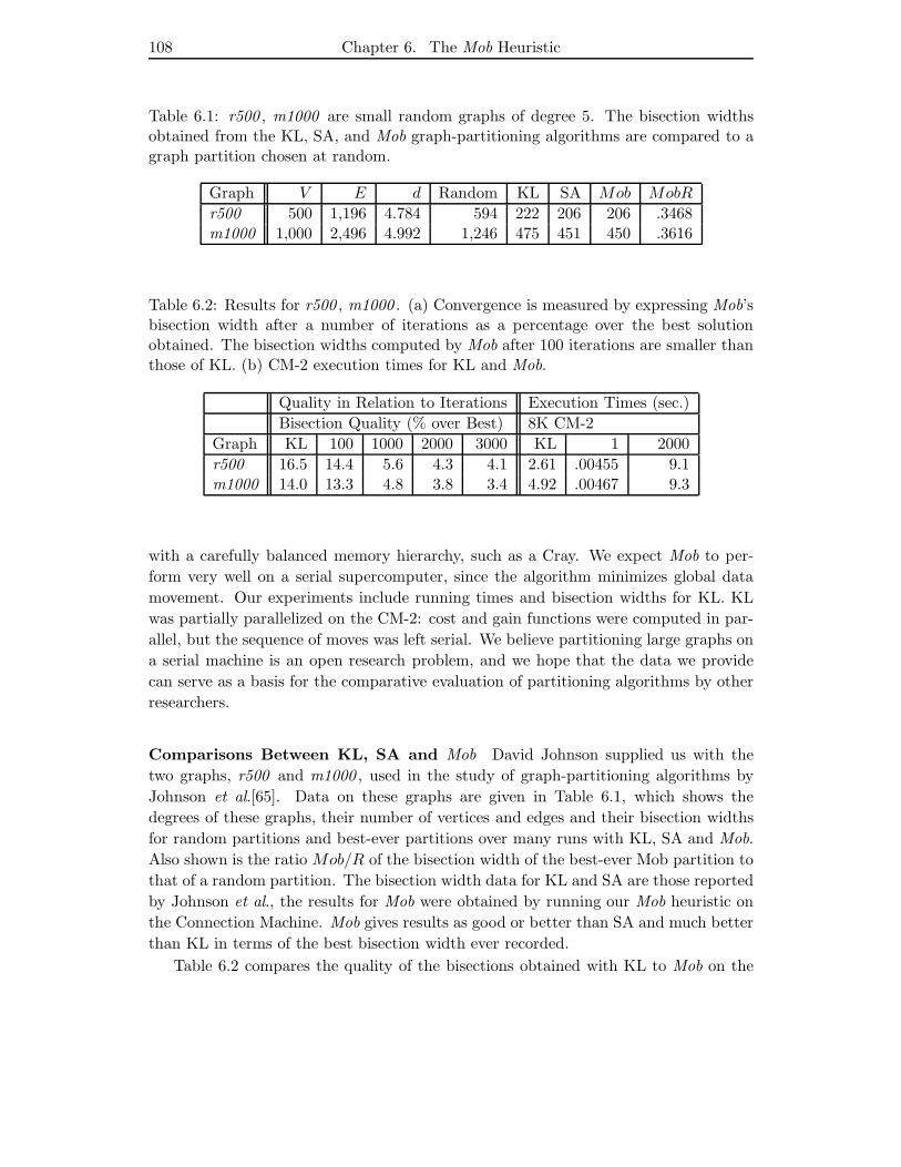
108 Chapter 6. The Mob Heuristic
Table 6.1: r500 , m1000 are small random graphs of degree 5. The bisection widthsobtained from the KL, SA, and Mob graph-partitioning algorithms are compared to agraph partition chosen at random.
Graph V E d Random KL SA Mob MobR
r500 500 1,196 4.784 594 222 206 206 .3468m1000 1,000 2,496 4.992 1,246 475 451 450 .3616
Table 6.2: Results for r500 , m1000 . (a) Convergence is measured by expressing Mob’sbisection width after a number of iterations as a percentage over the best solutionobtained. The bisection widths computed by Mob after 100 iterations are smaller thanthose of KL. (b) CM-2 execution times for KL and Mob.
Quality in Relation to Iterations Execution Times (sec.)
Bisection Quality (% over Best) 8K CM-2
Graph KL 100 1000 2000 3000 KL 1 2000
r500 16.5 14.4 5.6 4.3 4.1 2.61 .00455 9.1m1000 14.0 13.3 4.8 3.8 3.4 4.92 .00467 9.3
with a carefully balanced memory hierarchy, such as a Cray. We expect Mob to per-
form very well on a serial supercomputer, since the algorithm minimizes global data
movement. Our experiments include running times and bisection widths for KL. KL
was partially parallelized on the CM-2: cost and gain functions were computed in par-
allel, but the sequence of moves was left serial. We believe partitioning large graphs on
a serial machine is an open research problem, and we hope that the data we provide
can serve as a basis for the comparative evaluation of partitioning algorithms by other
researchers.
Comparisons Between KL, SA and Mob David Johnson supplied us with the
two graphs, r500 and m1000 , used in the study of graph-partitioning algorithms by
Johnson et al.[65]. Data on these graphs are given in Table 6.1, which shows the
degrees of these graphs, their number of vertices and edges and their bisection widths
for random partitions and best-ever partitions over many runs with KL, SA and Mob.
Also shown is the ratio Mob/R of the bisection width of the best-ever Mob partition to
that of a random partition. The bisection width data for KL and SA are those reported
by Johnson et al., the results for Mob were obtained by running our Mob heuristic on
the Connection Machine. Mob gives results as good or better than SA and much better
than KL in terms of the best bisection width ever recorded.
Table 6.2 compares the quality of the bisections obtained with KL to Mob on the
6.2. The Mob Graph-Partitioning Heuristic 109
basis of their execution times. We implemented KL on the Connection Machine by
modifying our implementation for Mob, and gave KL an advantage by computing the
bisection widths and vertex pair selected for a swap in parallel.
The first column labeled KL in Table 6.2 reports the percentage by which the
average width of a bisection found by our implementation of KL exceeds the best-ever
bisection size (with any heuristic) on r500 in 100 runs with randomly chosen initial
partitions and on m1000 in 400 runs. The columns labeled 100, 1000, 2000 and 3000
report the same data for Mob when the number of iterations (one iteration is the
swapping of two mobs) is that in the column header. It is a characteristic of Mob
that the bisection width it discovers improves as the number of swaps increases, while
the bisection width discovered by KL improves only by choosing increasing numbers
of random initial partitions, thereby increasing the odds that a good partition will be
found.
Table 6.2 also reports the average execution time for one iteration of KL and for
one and 2,000 iterations of Mob on an 8K-node CM-2 machine. The run times reflect
the fact that the graphs are too small to use the Connection Machine fully.
Large Random Graphs To calibrate Mob further, we conducted experiments on
randomly generated graphs with up to 1M vertices and 2M edges. Our random graphs
were generated by selecting pairs of vertices at random and removing multiple edges
and self-loops to yield a total of V d/2 edges. (We did not use the standard approach of
generating edges by flipping a coin with the appropriate probability for all V (V − 1)/2
potential edges in a graph because the number of trials would have been far too large.)
The graphs are of small average degree d, ranging from d = 3 . . . 16, since this is the kind
found in VLSI CAD and processor-mapping problems. SA and KL have prohibitive
running times for such large graphs. Consequently, we measure the quality of our
results primarily by comparing them among themselves, although we do report results
given by KL on 16K-vertex graphs and one 32K-vertex graph.
The number of edges and vertices and average degree of the random graphs in our
experiments are given in Table 6.3. We used seven graphs of degree 4 and seven graphs
of degree 8 to study the effect of increasing graph size on solution quality and running
time. We performed experiments on nine graphs with 16K vertices and degrees ranging
from 3 to 16 to examine the effect of graph degree on the behavior of the Mob algorithm.
This data was averaged over at least 10 runs.
Mob Schedule for Graph Partitioning The mob schedule specifies how many
vertices can swap at one iteration and thus influences how the Mob heuristic converges.
The mob schedule used for random graphs is constructed as follows: the maximum
mob size of the schedule is set to 10% of the number of vertices in the graph. The mob
size is then decremented to 0 in 40 uniform steps. The process is then repeated. Mob
was always stopped after 4000 iterations. We found that this schedule worked well with
graphs of varying size and degree.
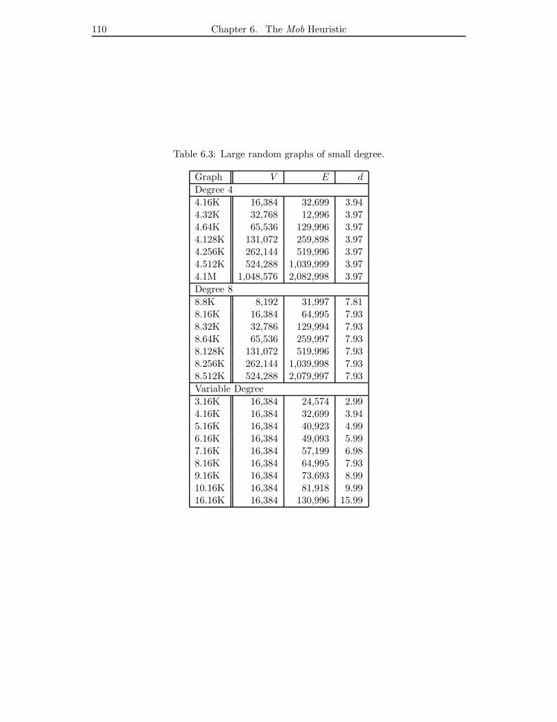
110 Chapter 6. The Mob Heuristic
Table 6.3: Large random graphs of small degree.
Graph V E d
Degree 4
4.16K 16,384 32,699 3.944.32K 32,768 12,996 3.974.64K 65,536 129,996 3.974.128K 131,072 259,898 3.974.256K 262,144 519,996 3.974.512K 524,288 1,039,999 3.974.1M 1,048,576 2,082,998 3.97
Degree 8
8.8K 8,192 31,997 7.818.16K 16,384 64,995 7.938.32K 32,786 129,994 7.938.64K 65,536 259,997 7.938.128K 131,072 519,996 7.938.256K 262,144 1,039,998 7.938.512K 524,288 2,079,997 7.93
Variable Degree
3.16K 16,384 24,574 2.994.16K 16,384 32,699 3.945.16K 16,384 40,923 4.996.16K 16,384 49,093 5.997.16K 16,384 57,199 6.988.16K 16,384 64,995 7.939.16K 16,384 73,693 8.9910.16K 16,384 81,918 9.9916.16K 16,384 130,996 15.99
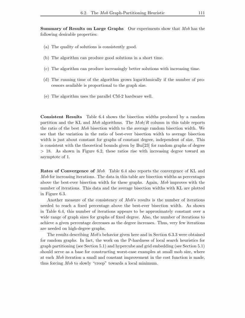
6.2. The Mob Graph-Partitioning Heuristic 111
Summary of Results on Large Graphs Our experiments show that Mob has the
following desirable properties:
(a) The quality of solutions is consistently good.
(b) The algorithm can produce good solutions in a short time.
(c) The algorithm can produce increasingly better solutions with increasing time.
(d) The running time of the algorithm grows logarithmically if the number of pro-
cessors available is proportional to the graph size.
(e) The algorithm uses the parallel CM-2 hardware well.
Consistent Results Table 6.4 shows the bisection widths produced by a random
partition and the KL and Mob algorithms. The Mob/R column in this table reports
the ratio of the best Mob bisection width to the average random bisection width. We
see that the variation in the ratio of best-ever bisection width to average bisection
width is just about constant for graphs of constant degree, independent of size. This
is consistent with the theoretical bounds given by Bui[23] for random graphs of degree
> 18. As shown in Figure 6.2, these ratios rise with increasing degree toward an
asymptote of 1.
Rates of Convergence of Mob Table 6.4 also reports the convergence of KL and
Mob for increasing iterations. The data in this table are bisection widths as percentages
above the best-ever bisection width for these graphs. Again, Mob improves with the
number of iterations. This data and the average bisection widths with KL are plotted
in Figure 6.3.
Another measure of the consistency of Mob’s results is the number of iterations
needed to reach a fixed percentage above the best-ever bisection width. As shown
in Table 6.4, this number of iterations appears to be approximately constant over a
wide range of graph sizes for graphs of fixed degree. Also, the number of iterations to
achieve a given percentage decreases as the degree increases. Thus, very few iterations
are needed on high-degree graphs.
The results describing Mob’s behavior given here and in Section 6.3.3 were obtained
for random graphs. In fact, the work on the P-hardness of local search heuristics for
graph partitioning (see Section 5.1) and hypercube and grid embedding (see Section 5.1)
should serve as a base for constructing worst-case examples at small mob size, where
at each Mob iteration a small and constant improvement in the cost function is made,
thus forcing Mob to slowly “creep” towards a local minimum.

112 Chapter 6. The Mob Heuristic
Table 6.4: Graph-partitioning results for large random graphs. The bisection widthsof the KL and Mob graph-partitioning algorithms are compared to a graph partitionchosen at random. Convergence is measured by expressing Mob’s bisection width aftera number of iterations as a percentage over the best solution obtained. The bisectionwidths computed by Mob after 100 iterations are smaller than those of KL.
Graph Bisections Bisection Quality (% over Best)
Graph Random KL Mob Mob/R KL 100 1000 2000 3000
Degree 4
4.16K 16,130 5,685 4,838 .2999 17.5 14.3 3.0 1.4 1.14.32K 32,224 11,477 9,824 .3049 16.8 13.2 3.2 2.8 1.04.64K 65,547 - 19,504 .2976 - 14.5 3.7 1.8 1.24.128K 131,173 - 39,010 .2974 - 14.7 4.2 1.8 0.94.256K 259,843 - 80,725 .3107 - 14.0 4.2 2.0 1.04.512K 520,538 - 156,294 .3003 - 14.4 4.8 2.1 1.34.1M 1,041,426 - 314,463 .3020 - 13.8 4.7 1.9 1.0
Degree 8
8.8K 16,013 8,100 7,716 .4819 5.0 5.8 1.5 1.0 0.98.16K 32,479 16,778 15,873 .4887 5.7 5.2 1.1 0.4 0.38.32K 64,991 33,924 31,670 .4873 7.1 5.4 1.3 0.7 0.58.64K 129,876 - 63,539 .4892 - 5.0 1.1 0.4 0.28.128K 260,034 - 127,003 .4884 - 5.1 1.2 0.5 0.28.256K 520,041 - 253,804 .4880 - 5.2 1.4 0.6 0.38.512K 1,039,073 - 507,824 .4887 - 5.1 1.4 0.6 0.2
Variable Degree
3.16K 12,290 3,402 2,653 .2159 28.2 22.8 5.3 3.0 2.14.16K 16,130 5,685 4,838 .2999 17.5 14.3 3.0 1.4 1.15.16K 20,443 8,482 7,520 .3679 12.9 10.3 2.1 1.1 0.96.16K 24,554 11,246 10,234 .4170 9.9 7.3 1.4 0.6 0.47.16K 28,608 14,212 13,030 .4555 9.1 6.4 1.6 0.8 0.78.16K 32,479 16,778 15,873 .4887 5.7 5.2 1.1 0.4 0.39.16K 36,865 20,123 19,046 .5166 5.7 4.4 1.0 0.5 0.310.16K 40,971 23,319 22,068 .5386 5.7 4.3 1.3 0.8 0.716.16K 65,517 42,722 41,324 .6307 3.4 2.7 0.7 0.4 0.3
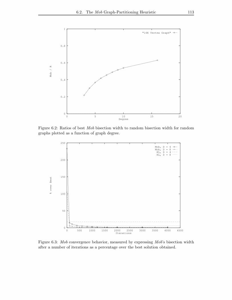
6.2. The Mob Graph-Partitioning Heuristic 113
0
0.2
0.4
0.6
0.8
1
0 5 10 15 20
Mob / R
Degree
"16K Vertex Graph"
Figure 6.2: Ratios of best Mob bisection width to random bisection width for randomgraphs plotted as a function of graph degree.
0
50
100
150
200
250
0 500 1000 1500 2000 2500 3000 3500 4000 4500
% over Best
Iterations
Mob, D = 4Mob, D = 8KL, D = 4KL, D = 8
Figure 6.3: Mob convergence behavior, measured by expressing Mob’s bisection widthafter a number of iterations as a percentage over the best solution obtained.

114 Chapter 6. The Mob Heuristic
Table 6.5: Timing results (sec.) for graph partitioning for large random graphs: exe-cution times were measured for KL on an 8K CM-2 and for 1 and 2000 Mob iterationson an 8K, 16K, and 32K CM-2.
8K CM-2 16K CM-2 32K CM-2
Degree 4
Graph 1 KL 1 2000 1 2000 1 2000
4.16K - .0175 35.0 .0106 21.2 - -4.32K - .0331 70.2 .0188 37.6 .0100 20.04.64K - .0650 130.0 .0347 69.4 .0220 44.04.128K - .1262 252.4 .0660 132.0 .0361 72.24.256K - .2469 493.8 .1277 255.4 .0669 133.84.512K - - - .2674 534.8 .1316 267.24.1M - - - - - .2597 519.4
Degree 8
8.8K 433 .0185 37.0 .0105 21.0 .0065 138.16K 1445 .0320 64.0 .0186 37.2 .0103 20.68.32K 4000 .0601 120.2 .0348 69.6 .0199 39.88.64K - .1230 246.0 .0730 146.0 .0360 72.08.128K - .2448 489.6 .1295 259.0 .0674 134.88.256K - - - .2610 522.0 .1298 259.68.512K - - - - - .2581 516.2
Variable Degree
3.16K - .0173 34.6 .0103 20.6 - -4.16K - .0175 35.0 .0106 21.2 - -5.16K 983 .0330 66.0 .0190 38.0 .0120 24.06.16K 961 .0362 72.4 .0179 35.8 .0101 20.27.16K 1266 .0340 68.0 .0183 36.6 .0102 20.48.16K 1444 .0320 64.0 .0186 37.2 .0103 20.69.16K 940 .0610 122.0 .0331 66.2 .0191 38.210.16K 1741 .0660 132.0 .0329 65.8 .0192 38.416.16K 1998 .0637 127.4 .0351 70.2 .0203 40.6
6.2. The Mob Graph-Partitioning Heuristic 115
Computation Time We also experimented with graphs of different sizes on ma-
chines with varying numbers of real processors. The results of these experiments are
reported in Table 6.5. We find that the time per iteration normalized by the num-
ber of virtual processors is nearly constant on the Connection Machine. That is, our
heuristic runs in nearly constant time per edge. For the largest graphs with 2M edges,
we used 4M virtual processors. Since the graph size that can be handled on the CM-2
is bounded by the memory required for each virtual processor, as more real proces-
sors and memory are added, execution times should keep decreasing and bisections of
increasingly larger graphs can be computed.
The absolute speed at which a bisection is produced by Mob is remarkable: On a
32K CM-2, a bisection of a 1M-vertex, 2M-edge random graph that is within 2 percent
of optimal is found in 520 seconds (less than 9 minutes).
116 Chapter 6. The Mob Heuristic
6.3 The Mob Graph-Embedding Heuristic
We modified the Mob heuristic for graph partitioning described in Section 6.2 and
applied it to grid and hypercube embedding. The performance of the Mob heuristics
was evaluated by an extensive series of experiments on the Connection Machine CM-
2[119,125]. The Mob neighborhood for grid and hypercube embedding is described
in Section 6.3.1, and the details of the implementation are given in Section 6.3.2. In
Section 6.3.3 and 6.3.4 we describe experiments with Mob. 1-to-1 mappings of graph
vertices to network nodes were used to model VLSI placement problems and standard
embedding problems and 16-to-1 mappings were chosen to model bulk parallelism. We
conducted experiments on randomly generated graphs of small (d = 3 . . . 16) degrees
with up to 500K vertices and 1M edges. On random graphs, the parallel complexity
of the Mob heuristic on the CM-2 was found to be time O(log |E|) with 2|E| proces-
sors. The absolute speed at which an embedding is produced shows that Mob can be
implemented very efficiently on a SIMD-style machine. Due to excessive run times,
heuristics previously reported in the literature can construct graph embeddings only
for graphs 100 to 1000 times smaller than those used in our experiments.
6.3.1 The Mob Neighborhood for Graph Embedding
The Mob heuristic for graph partitioning introduced in Section 6.2.1 is the basis for
our graph-embedding heuristics. We report on two new Mob heuristics for embedding
graphs into two-dimensional grid and hypercube networks. We now define the mob-
neighborhood MOB-N(S,m) structure for graph embedding.
Definition 26 The mob neighborhood MOB-N(S,m) of an embedding S is the set of
embeddings obtained from S by swapping m pairs of vertices.
The size of MOB-N(S,m) is n!(n−2m)!m! . Clearly, it is not feasible to compute the
gains of all embeddings in the neighborhood MOB-N(S,m) of a solution S. If we were to
pick an embedding S at random from MOB-N(S,m), we should expect only a very small
change in the cost function on average. Therefore, for grid and hypercube embeddings
we use the neighborhood MOB-NR(S,m, d), a restriction of the mob-neighborhood
MOB-N(S,m) that uses the mob-selection rule MOB-R given below to look for a rough
approximation to the subset that causes the largest improvement in the embedding
cost.
We can approximate the gain of swapping m pairs of vertices by adding the gains
of the vertex swaps. For every embedding,(|V1|
2
)
individual vertex swaps are possi-
ble. The processor-time cost of proposing all possible vertex swaps, computing their
gains, and then using the mob procedure to pick the swaps with the best gain, while
ensuring that swaps do not share vertices, would be O(|V1|2); this would be a waste of
computational resources and inappropriate for the graphs in our experiments, where
|V1| > 106. We want to generate an O(|V1|)-size subset of all possible vertex swaps.
6.3. The Mob Graph-Embedding Heuristic 117
A subset of size O(|V1|) swaps picked at random from the set of all possible swaps
will probably not contain a very large number of possible high-gain swaps. Therefore,
on the hypercube, a hypercube axis d is chosen at random and vertices are swapped
between hypercube neighbors across the chosen hypercube axis. On the grid, a dis-
tance d of ±1, 2, 4, 8, 16, . . . on either the X or Y axis is chosen at random and vertices
are swapped between grid nodes that have separation d. We make the meaning of
separation d unambiguous to rule out that a grid node swaps vertices with two other
nodes:
Definition 27 Let i(v) be the coordinate of a node in a linear array, grid axis or
hypercube. Let (v,w) be a pair of nodes with i(v) < i(w). On the linear array or grid
axis, the node pair (v,w) has separation d if |i(v)− i(w)| = |d|, and if ⌈i(v)/|d|⌉ is even
when d is positive, or if ⌈i(v)/|d|⌉ is odd when d is negative. On the hypercube, the
node pair (v,w) has separation d if the coordinates i(v) and i(w) differ in the dth bit.
This move set is geared to the communication bottlenecks of the underlying com-
puting network; its effect is that, while a vertex may not be able to move to its optimal
position in one step, it can approach this position in a very small number of steps.
Definition 28 The mob neighborhood MOB-NR(S,m, d) of an embedding S is the set
of embeddings obtained from S by selecting m pairs of vertices with separation d in
the network with the MOB-R rule and swapping these vertices.
Definition 29 The rule MOB-R(S,m, r1, r2, d) selects a mob of size m as follows: let
r1, r2 be random real numbers drawn uniformly from the interval (0, 1). For each
vertex pair (v,w) that have separation d in the network, let gain(v,w) be the change
in the embedding cost if v and w are swapped, and let gain(v,w) be positive if the
embedding cost decreases. Let SX(g) = v ∈ X | gain(v,w) ≥ g. Choose gX such
that |SX(gX + 1)| < m ≤ |SX(gX )|. Let mp = |SX(gX)| be the size of the pre-mob
SX(gX ). Each element in SX(gX ) is indexed from 0 to mp − 1. A mob of size m is
selected from SX(gX) by adding ⌊r1mp⌋ to each index modulo mp and selecting those
with index less than m.
The rule MOB-R(S,m, r1, r2, d) selects a group of high-gain vertices of size mob to
move a distance d. To avoid sorting by gain, we use an adaptive binary search algorithm
to identify a pre-mob of vertices with gain g or larger in each set of the embedding,
where g is the smallest gain for which at least mob vertices have a gain greater than or
equal to g. We select mob vertices at random from this pre-mob.
We also implemented routines to choose exactly m vertices whose individual gains
are largest, but neither sorting or randomized methods provided adequate performance.
Instead we choose vertices at random among all vertices in SX(gX). While in so doing
we may miss some vertices with large gain, our heuristic is very effective.
118 Chapter 6. The Mob Heuristic
6.3.2 Implementation of Mob
We now discuss how the Mob grid-and hypercube-embedding heuristic was implemented
to make full use of the CM-2’s parallel hardware and instruction set. Since the heuris-
tics are closely related to the Mob graph-partitioning heuristic, we do not repeat the
description in Section 6.2.2 of operations common to both types of the Mob heuristic.
We used the same edge data structure as for the Mob graph-partitioning heuristic. The
operations of computing cost, gain, selecting a mob from a pre-mob, and exchanging
vertices are identical to the operations used for graph-partitioning, and are described
in Section 6.2.2. The move-generation routine limits the size of the neighborhood of an
embedding in order to use a reasonable number of processors and still allow the Mob
heuristic to converge quickly to a good solution. We show how to construct a vertex
data structures that can exchange vertices with minimal communication overhead.
Move Generation When more than one vertex is embedded on a network node,
ordering the vertices on a network node by their gain generates swaps with higher added
gains. We have found that this significantly speeds up the convergence behavior of the
Mob heuristic. We experimented with several move-generating procedures and found
that the cost of sorting vertex gains, segmented by the network nodes, is prohibitive on
the CM-2. We therefore implemented a compromise in which every network node finds
the vertex with highest gain and swaps it into the first location of the node segment
in the vertex array. We believe that this max-gain shuffle offers an excellent trade-off
between computation time and convergence behavior.
Vertex Data Structure The number of vertices at a network node must remain
constant to ensure correct operation of our heuristic. Therefore, after every vertex has
computed its gain, a separate vertex data structure is used to form pairs of vertices to
be swapped. (This data structure was not needed for the graph-partitioning heuristic
in Section 6.2.2, since it was not necessary to form vertex pairs to be swapped.) The
vertices are stored in a linear array, and the edge data structure maintains link pointers
to the vertex processors. The vertex data structure is designed to facilitate rapid vertex
exchanges. Vertices embedded on the same network node are adjacent in the vertex
array. Filler vertices are added at the initialization stage of the Mob heuristic to ensure
that every network node has the same number of embedded vertices. Let V1 be the
number of vertices to be embedded, |V2| the number of network nodes, and k = |V1|/|V2|the number of embedded vertices per node. Every network node can communicate and
swap vertices with a network node a distance d away by simply adding kd modulo
|V2| to its own address in the vertex array. Such monotonic communication patterns
are asymptotically easier to route on most architectures than general patterns. For
instance, the pattern can be implemented by a chain of nearest-neighbor communication
operations on the hypercube network of the Connection Machine.
6.3. The Mob Graph-Embedding Heuristic 119
We experimented with an alternative method of generating vertex swaps, that re-
quires only the edge data structure. Each vertex processor, represented by the first
edge processor in the edge data structure, computes the address of the network node
to which it will move. Computing the address of this target node is a simple arithmetic
operation. To form a pair of vertices to be swapped, the vertex at the target node
has to be located in the edge data structure; this is an operation not easily supported
by the edge data structure. One easy solution is to sort the vertices by their target
addresses. We concluded that the cost of transferring information to and from the
vertex data structure was an order of magnitude smaller than the cost of sorting node
addresses, and gave us a more flexible data structure.
6.3.3 Experimental Results for Random Graphs
We evaluated the performance of the Mob hypercube and grid-embedding algorithms
by conducting experiments on the CM-2. 1-to-1 mappings of graph vertices to network
nodes were used to model VLSI placement problems and standard embedding problems.
We also wanted to model bulk parallelism, where n virtual processors are embedded
into a computing network of size n/ log n, and chose 16-to-1 mappings as a rough
approximation of log n-to-1 mappings. The random graphs studied here are more than
1000 times larger than graphs previously studied in the literature. Serial algorithms
such as SA or KL would have prohibitive running times for such large graphs. We
measured the solution quality, convergence as a function of time, and running times
with a varying number of processors, and compared Mob to other algorithms. The
Mob embedding heuristics produce excellent solutions, converge quickly, run in time
O(log |E|) with 2|E| processors, and are well matched to the parallel CM-2 hardware.
We conducted experiments on randomly generated graphs with up to 512K vertices
and 1M edges. (See Section 6.2.3 on how these graphs were generated.) The number of
edges, vertices and average degree of the random graphs used in our experiments are
the same as used for graph partitioning, and are given in Table 6.3 in Section 6.2.3.
We used six graphs of average degree 4 and six graphs of average degree 8 to study
the effect of increasing graph size on solution quality and running time. We performed
experiments on nine graphs with 16K vertices and average degrees ranging from 3 to
16 to examine the effect of graph degree on the behavior of the Mob algorithms. The
data was averaged over at least five runs.
Mob Schedule for Graph Embedding The mob schedule specifies how many ele-
ment pairs can swap at one iteration, and thus influences how the grid and hypercube
Mob heuristic converges. The mob schedule used for random graphs is constructed as
follows: the maximum mob size of the schedule is set to the number of vertex pairs
divided by 8. The mob size is then decremented in 16 uniform steps. The process is
repeated, doubling the number of steps required to decrement the mob size from the
maximum value every time. Mob was always stopped after 8000 iterations.
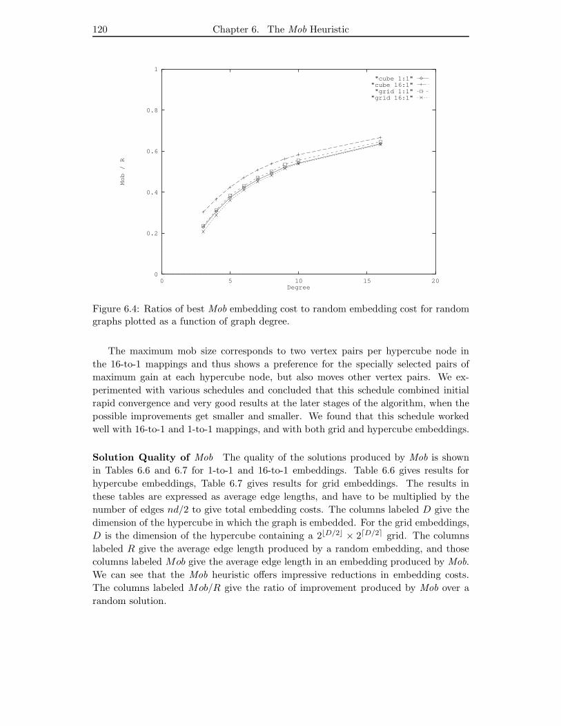
120 Chapter 6. The Mob Heuristic
0
0.2
0.4
0.6
0.8
1
0 5 10 15 20
Mob / R
Degree
"cube 1:1""cube 16:1""grid 1:1""grid 16:1"
Figure 6.4: Ratios of best Mob embedding cost to random embedding cost for randomgraphs plotted as a function of graph degree.
The maximum mob size corresponds to two vertex pairs per hypercube node in
the 16-to-1 mappings and thus shows a preference for the specially selected pairs of
maximum gain at each hypercube node, but also moves other vertex pairs. We ex-
perimented with various schedules and concluded that this schedule combined initial
rapid convergence and very good results at the later stages of the algorithm, when the
possible improvements get smaller and smaller. We found that this schedule worked
well with 16-to-1 and 1-to-1 mappings, and with both grid and hypercube embeddings.
Solution Quality of Mob The quality of the solutions produced by Mob is shown
in Tables 6.6 and 6.7 for 1-to-1 and 16-to-1 embeddings. Table 6.6 gives results for
hypercube embeddings, Table 6.7 gives results for grid embeddings. The results in
these tables are expressed as average edge lengths, and have to be multiplied by the
number of edges nd/2 to give total embedding costs. The columns labeled D give the
dimension of the hypercube in which the graph is embedded. For the grid embeddings,
D is the dimension of the hypercube containing a 2⌊D/2⌋ × 2⌈D/2⌉ grid. The columns
labeled R give the average edge length produced by a random embedding, and those
columns labeled Mob give the average edge length in an embedding produced by Mob.
We can see that the Mob heuristic offers impressive reductions in embedding costs.
The columns labeled Mob/R give the ratio of improvement produced by Mob over a
random solution.
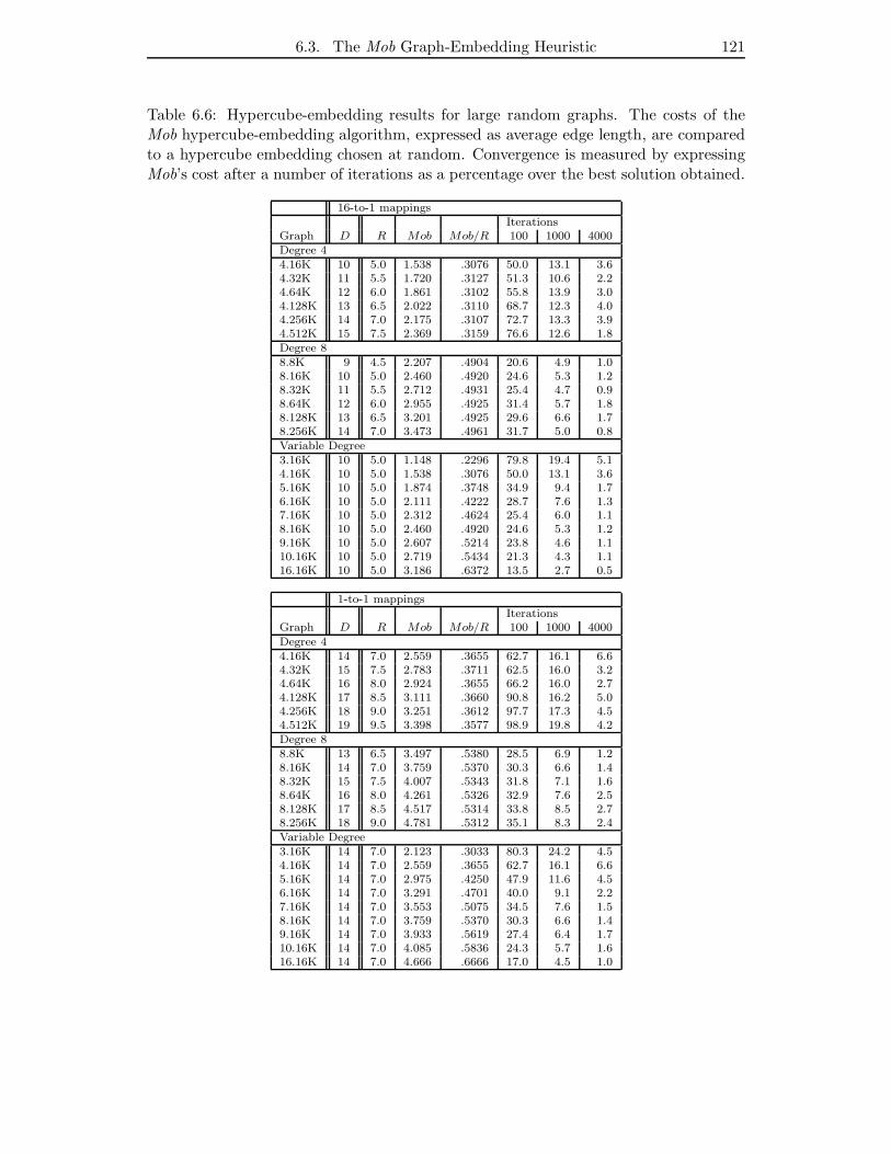
6.3. The Mob Graph-Embedding Heuristic 121
Table 6.6: Hypercube-embedding results for large random graphs. The costs of theMob hypercube-embedding algorithm, expressed as average edge length, are comparedto a hypercube embedding chosen at random. Convergence is measured by expressingMob’s cost after a number of iterations as a percentage over the best solution obtained.
16-to-1 mappingsIterations
Graph D R Mob Mob/R 100 1000 4000Degree 44.16K 10 5.0 1.538 .3076 50.0 13.1 3.64.32K 11 5.5 1.720 .3127 51.3 10.6 2.24.64K 12 6.0 1.861 .3102 55.8 13.9 3.04.128K 13 6.5 2.022 .3110 68.7 12.3 4.04.256K 14 7.0 2.175 .3107 72.7 13.3 3.94.512K 15 7.5 2.369 .3159 76.6 12.6 1.8Degree 88.8K 9 4.5 2.207 .4904 20.6 4.9 1.08.16K 10 5.0 2.460 .4920 24.6 5.3 1.28.32K 11 5.5 2.712 .4931 25.4 4.7 0.98.64K 12 6.0 2.955 .4925 31.4 5.7 1.88.128K 13 6.5 3.201 .4925 29.6 6.6 1.78.256K 14 7.0 3.473 .4961 31.7 5.0 0.8Variable Degree3.16K 10 5.0 1.148 .2296 79.8 19.4 5.14.16K 10 5.0 1.538 .3076 50.0 13.1 3.65.16K 10 5.0 1.874 .3748 34.9 9.4 1.76.16K 10 5.0 2.111 .4222 28.7 7.6 1.37.16K 10 5.0 2.312 .4624 25.4 6.0 1.18.16K 10 5.0 2.460 .4920 24.6 5.3 1.29.16K 10 5.0 2.607 .5214 23.8 4.6 1.110.16K 10 5.0 2.719 .5434 21.3 4.3 1.116.16K 10 5.0 3.186 .6372 13.5 2.7 0.5
1-to-1 mappingsIterations
Graph D R Mob Mob/R 100 1000 4000Degree 44.16K 14 7.0 2.559 .3655 62.7 16.1 6.64.32K 15 7.5 2.783 .3711 62.5 16.0 3.24.64K 16 8.0 2.924 .3655 66.2 16.0 2.74.128K 17 8.5 3.111 .3660 90.8 16.2 5.04.256K 18 9.0 3.251 .3612 97.7 17.3 4.54.512K 19 9.5 3.398 .3577 98.9 19.8 4.2Degree 88.8K 13 6.5 3.497 .5380 28.5 6.9 1.28.16K 14 7.0 3.759 .5370 30.3 6.6 1.48.32K 15 7.5 4.007 .5343 31.8 7.1 1.68.64K 16 8.0 4.261 .5326 32.9 7.6 2.58.128K 17 8.5 4.517 .5314 33.8 8.5 2.78.256K 18 9.0 4.781 .5312 35.1 8.3 2.4Variable Degree3.16K 14 7.0 2.123 .3033 80.3 24.2 4.54.16K 14 7.0 2.559 .3655 62.7 16.1 6.65.16K 14 7.0 2.975 .4250 47.9 11.6 4.56.16K 14 7.0 3.291 .4701 40.0 9.1 2.27.16K 14 7.0 3.553 .5075 34.5 7.6 1.58.16K 14 7.0 3.759 .5370 30.3 6.6 1.49.16K 14 7.0 3.933 .5619 27.4 6.4 1.710.16K 14 7.0 4.085 .5836 24.3 5.7 1.616.16K 14 7.0 4.666 .6666 17.0 4.5 1.0
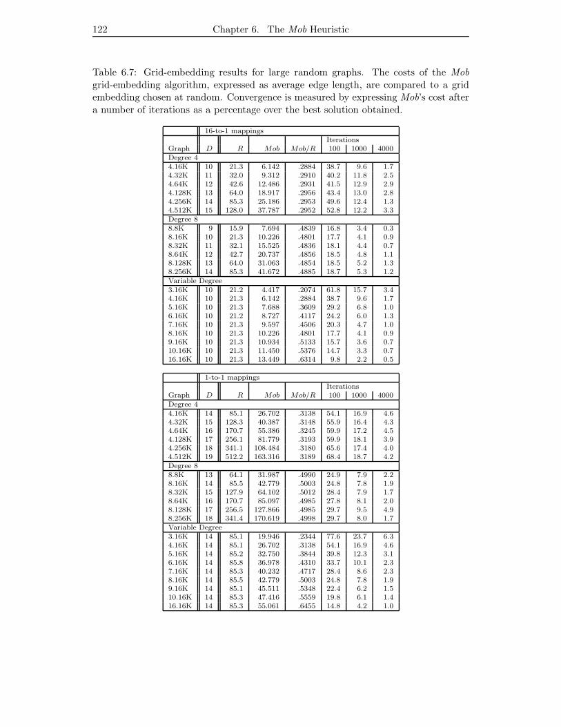
122 Chapter 6. The Mob Heuristic
Table 6.7: Grid-embedding results for large random graphs. The costs of the Mobgrid-embedding algorithm, expressed as average edge length, are compared to a gridembedding chosen at random. Convergence is measured by expressing Mob’s cost aftera number of iterations as a percentage over the best solution obtained.
16-to-1 mappingsIterations
Graph D R Mob Mob/R 100 1000 4000Degree 44.16K 10 21.3 6.142 .2884 38.7 9.6 1.74.32K 11 32.0 9.312 .2910 40.2 11.8 2.54.64K 12 42.6 12.486 .2931 41.5 12.9 2.94.128K 13 64.0 18.917 .2956 43.4 13.0 2.84.256K 14 85.3 25.186 .2953 49.6 12.4 1.34.512K 15 128.0 37.787 .2952 52.8 12.2 3.3Degree 88.8K 9 15.9 7.694 .4839 16.8 3.4 0.38.16K 10 21.3 10.226 .4801 17.7 4.1 0.98.32K 11 32.1 15.525 .4836 18.1 4.4 0.78.64K 12 42.7 20.737 .4856 18.5 4.8 1.18.128K 13 64.0 31.063 .4854 18.5 5.2 1.38.256K 14 85.3 41.672 .4885 18.7 5.3 1.2Variable Degree3.16K 10 21.2 4.417 .2074 61.8 15.7 3.44.16K 10 21.3 6.142 .2884 38.7 9.6 1.75.16K 10 21.3 7.688 .3609 29.2 6.8 1.06.16K 10 21.2 8.727 .4117 24.2 6.0 1.37.16K 10 21.3 9.597 .4506 20.3 4.7 1.08.16K 10 21.3 10.226 .4801 17.7 4.1 0.99.16K 10 21.3 10.934 .5133 15.7 3.6 0.710.16K 10 21.3 11.450 .5376 14.7 3.3 0.716.16K 10 21.3 13.449 .6314 9.8 2.2 0.5
1-to-1 mappingsIterations
Graph D R Mob Mob/R 100 1000 4000Degree 44.16K 14 85.1 26.702 .3138 54.1 16.9 4.64.32K 15 128.3 40.387 .3148 55.9 16.4 4.34.64K 16 170.7 55.386 .3245 59.9 17.2 4.54.128K 17 256.1 81.779 .3193 59.9 18.1 3.94.256K 18 341.1 108.484 .3180 65.6 17.4 4.04.512K 19 512.2 163.316 3189 68.4 18.7 4.2Degree 88.8K 13 64.1 31.987 .4990 24.9 7.9 2.28.16K 14 85.5 42.779 .5003 24.8 7.8 1.98.32K 15 127.9 64.102 .5012 28.4 7.9 1.78.64K 16 170.7 85.097 .4985 27.8 8.1 2.08.128K 17 256.5 127.866 .4985 29.7 9.5 4.98.256K 18 341.4 170.619 .4998 29.7 8.0 1.7Variable Degree3.16K 14 85.1 19.946 .2344 77.6 23.7 6.34.16K 14 85.1 26.702 .3138 54.1 16.9 4.65.16K 14 85.2 32.750 .3844 39.8 12.3 3.16.16K 14 85.8 36.978 .4310 33.7 10.1 2.37.16K 14 85.3 40.232 .4717 28.4 8.6 2.38.16K 14 85.5 42.779 .5003 24.8 7.8 1.99.16K 14 85.1 45.511 .5348 22.4 6.2 1.510.16K 14 85.3 47.416 .5559 19.8 6.1 1.416.16K 14 85.3 55.061 .6455 14.8 4.2 1.0
6.3. The Mob Graph-Embedding Heuristic 123
Our experiments show:
(a) For fixed degree d, Mob/R is largely independent of graph size.
(b) 16-to-1 mappings give slightly better Mob/R ratios than 1-to-1 mappings. When
communication costs are modeled by edge lengths, this shows the advantage of
the bulk-parallel model in reducing overall network-communication bandwidth.
(c) The grid-embedding Mob heuristic achieves lower Mob/R ratios than the hyper-
cube Mob heuristic.
(d) The ratio Mob/R rises with increasing average graph degree toward an asymptote
of 1, as shown in Figure 6.4. The differences between grid and hypercube embed-
dings and between 1-to-1 and 16-to-1 embeddings become smaller with increasing
graph degree.
Rates of Convergence of Mob Tables 6.6 and 6.7 also report the convergence of
Mob for an increasing number of iterations. The columns labeled Iterations show the
average embedding cost as percentages above the best-ever embedding cost, produced
after 100, 1000 and 4000 iterations of Mob, respectively. Our experiments indicate
that the number of iterations needed to reach a fixed percentage above the best-ever
embedding cost appears to be approximately constant, and therefore independent of
graph size or network size. This important observation holds for hypercube and grid
embeddings and for 1-to-1 and 16-to-1 mappings. The behavior is surprising, since
vertices must travel larger distances, especially in grid networks, to reduce average edge
costs by a fixed ratio; it points out the importance and appropriateness of Mob’s set of
moves along hypercube axes. The fact that Mob’s rate of convergence is independent
of graph size was also observed for graph partitioning (see Section 6.2.3).
The Iterations columns in Tables 6.6 and 6.7 show that the reductions in embedding
costs decrease rapidly as the total number of iterations increases. The rate of conver-
gence is shown in Figure 6.5 for 16-to-1 mappings of the Mob grid and hypercube-
embedding algorithms. Thus, a good solution is produced rapidly; further improve-
ments can be obtained if enough computation time is available. Also, the number of
iterations to achieve a given percentage decreases as the degree increases, as seen in
Figure 6.5. Thus, fewer iterations are needed on high-degree graphs.
Computation Time The edge and vertex data structures are never used at the same
time in the Mob heuristic. The edge data structure, the larger of the two, requires 2|E|processors. The scan operations are the most complex operations in an iteration of
Mob. Thus, one iteration of Mob should run in time O(log |E|). This was tested by
experiments on the CM-2 with graphs of different sizes, in which the number of real
processors varied between 8K and 32K and the number of virtual (simulated) processors
ranged between 16K and 2M.
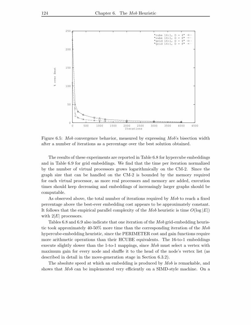
124 Chapter 6. The Mob Heuristic
0
50
100
150
200
250
0 500 1000 1500 2000 2500 3000 3500 4000 4500
% over Best
Iterations
"cube 16:1, D = 4""cube 16:1, D = 8""grid 16:1, D = 4""grid 16:1, D = 8"
Figure 6.5: Mob convergence behavior, measured by expressing Mob’s bisection widthafter a number of iterations as a percentage over the best solution obtained.
The results of these experiments are reported in Table 6.8 for hypercube embeddings
and in Table 6.9 for grid embeddings. We find that the time per iteration normalized
by the number of virtual processors grows logarithmically on the CM-2. Since the
graph size that can be handled on the CM-2 is bounded by the memory required
for each virtual processor, as more real processors and memory are added, execution
times should keep decreasing and embeddings of increasingly larger graphs should be
computable.
As observed above, the total number of iterations required by Mob to reach a fixed
percentage above the best-ever embedding cost appears to be approximately constant.
It follows that the empirical parallel complexity of the Mob heuristic is time O(log |E|)with 2|E| processors.
Tables 6.8 and 6.9 also indicate that one iteration of the Mob grid-embedding heuris-
tic took approximately 40-50% more time than the corresponding iteration of the Mob
hypercube-embedding heuristic, since the PERIMETER cost and gain functions require
more arithmetic operations than their HCUBE equivalents. The 16-to-1 embeddings
execute slightly slower than the 1-to-1 mappings, since Mob must select a vertex with
maximum gain for every node and shuffle it to the head of the node’s vertex list (as
described in detail in the move-generation stage in Section 6.3.2).
The absolute speed at which an embedding is produced by Mob is remarkable, and
shows that Mob can be implemented very efficiently on a SIMD-style machine. On a
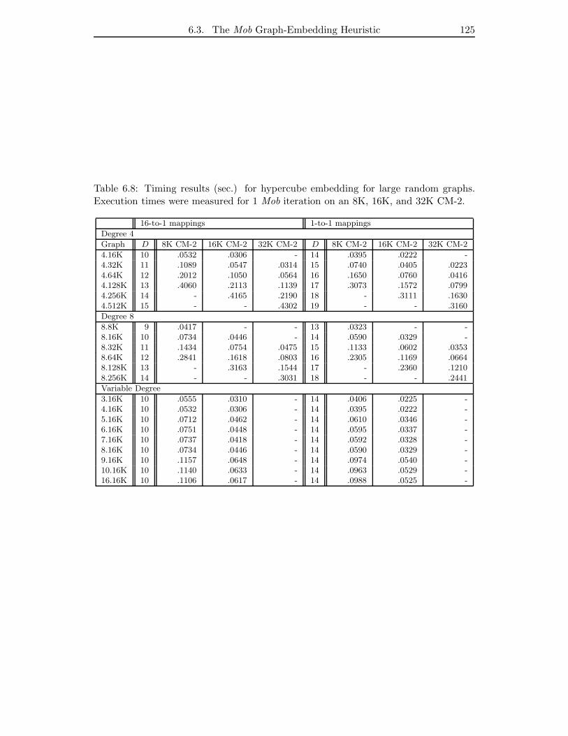
6.3. The Mob Graph-Embedding Heuristic 125
Table 6.8: Timing results (sec.) for hypercube embedding for large random graphs.Execution times were measured for 1 Mob iteration on an 8K, 16K, and 32K CM-2.
16-to-1 mappings 1-to-1 mappings
Degree 4
Graph D 8K CM-2 16K CM-2 32K CM-2 D 8K CM-2 16K CM-2 32K CM-2
4.16K 10 .0532 .0306 - 14 .0395 .0222 -4.32K 11 .1089 .0547 .0314 15 .0740 .0405 .02234.64K 12 .2012 .1050 .0564 16 .1650 .0760 .04164.128K 13 .4060 .2113 .1139 17 .3073 .1572 .07994.256K 14 - .4165 .2190 18 - .3111 .16304.512K 15 - - .4302 19 - - .3160
Degree 8
8.8K 9 .0417 - - 13 .0323 - -8.16K 10 .0734 .0446 - 14 .0590 .0329 -8.32K 11 .1434 .0754 .0475 15 .1133 .0602 .03538.64K 12 .2841 .1618 .0803 16 .2305 .1169 .06648.128K 13 - .3163 .1544 17 - .2360 .12108.256K 14 - - .3031 18 - - .2441
Variable Degree
3.16K 10 .0555 .0310 - 14 .0406 .0225 -4.16K 10 .0532 .0306 - 14 .0395 .0222 -5.16K 10 .0712 .0462 - 14 .0610 .0346 -6.16K 10 .0751 .0448 - 14 .0595 .0337 -7.16K 10 .0737 .0418 - 14 .0592 .0328 -8.16K 10 .0734 .0446 - 14 .0590 .0329 -9.16K 10 .1157 .0648 - 14 .0974 .0540 -10.16K 10 .1140 .0633 - 14 .0963 .0529 -16.16K 10 .1106 .0617 - 14 .0988 .0525 -
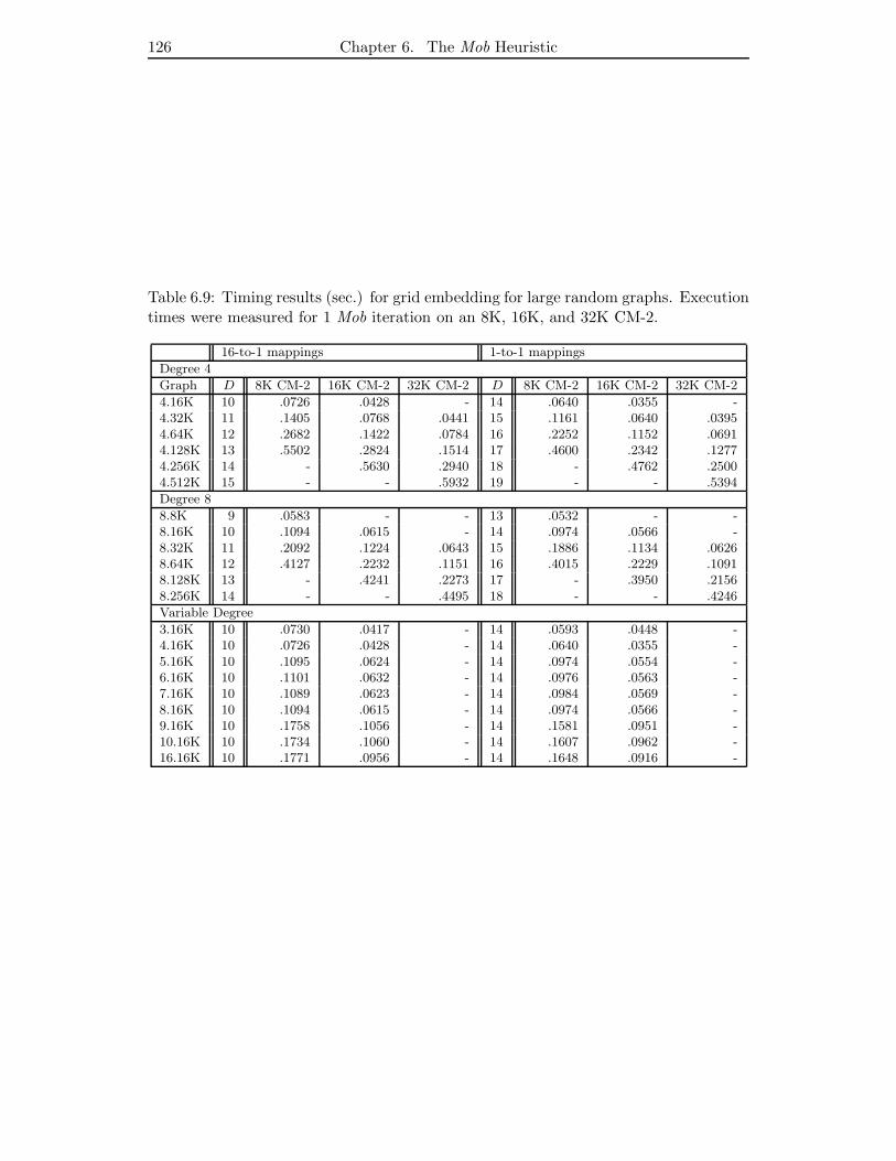
126 Chapter 6. The Mob Heuristic
Table 6.9: Timing results (sec.) for grid embedding for large random graphs. Executiontimes were measured for 1 Mob iteration on an 8K, 16K, and 32K CM-2.
16-to-1 mappings 1-to-1 mappings
Degree 4
Graph D 8K CM-2 16K CM-2 32K CM-2 D 8K CM-2 16K CM-2 32K CM-2
4.16K 10 .0726 .0428 - 14 .0640 .0355 -4.32K 11 .1405 .0768 .0441 15 .1161 .0640 .03954.64K 12 .2682 .1422 .0784 16 .2252 .1152 .06914.128K 13 .5502 .2824 .1514 17 .4600 .2342 .12774.256K 14 - .5630 .2940 18 - .4762 .25004.512K 15 - - .5932 19 - - .5394
Degree 8
8.8K 9 .0583 - - 13 .0532 - -8.16K 10 .1094 .0615 - 14 .0974 .0566 -8.32K 11 .2092 .1224 .0643 15 .1886 .1134 .06268.64K 12 .4127 .2232 .1151 16 .4015 .2229 .10918.128K 13 - .4241 .2273 17 - .3950 .21568.256K 14 - - .4495 18 - - .4246
Variable Degree
3.16K 10 .0730 .0417 - 14 .0593 .0448 -4.16K 10 .0726 .0428 - 14 .0640 .0355 -5.16K 10 .1095 .0624 - 14 .0974 .0554 -6.16K 10 .1101 .0632 - 14 .0976 .0563 -7.16K 10 .1089 .0623 - 14 .0984 .0569 -8.16K 10 .1094 .0615 - 14 .0974 .0566 -9.16K 10 .1758 .1056 - 14 .1581 .0951 -10.16K 10 .1734 .1060 - 14 .1607 .0962 -16.16K 10 .1771 .0956 - 14 .1648 .0916 -
6.3. The Mob Graph-Embedding Heuristic 127
32K CM-2 it takes approximately 1720 seconds (≈ 29 minutes) to find an embedding
of a 500K-vertex, 1M-edge graph into a 15-dimensional hypercube, and approximately
1264 seconds (≈ 21 minutes) to embed that graph into a 19-dimensional hypercube.
It takes approximately 2370 seconds (≈ 40 minutes) to find an embedding of a 500K-
vertex, 1M-edge graph into a 256 × 64 grid, and approximately 2157 seconds (≈ 36
minutes) to embed that graph into a 1024× 512 grid. All these embeddings are within
5 percent of best-ever.
Comparison to Graph-partitioning Algorithms To calibrate our results, we
measured the graph partitions produced by the hypercube and grid embeddings. A
graph embedding S is a mapping of graph vertices to network nodes. S is completely
described by storing for every vertex v the network node on which v is embedded. In the
implementation of Mob, this node field contains the hypercube address of the network
node, this is used directly for hypercube embeddings, and from it x, y-coordinates are
computed for grid embeddings. A graph partition P = (X,Y ) can be generated from
an embedding S by cutting the embedding in half along a hyperplane. A bit position
is selected in the node field, and all vertices with a 0 in that bit position are placed
in set X of the partition P , and all vertices with a 1 in that bit position are placed
in set Y . A d-dimensional hypercube network has d hyperplanes and thus d projected
partitions from which we can choose the partition with minimum cost. For hypercube
embeddings, we found that the cost of the projected partitions, measured by the number
of edges between the two sets, is about the same for all cutting hyperplanes. For grid
embeddings, the two hyperplanes corresponding to vertical and horizontal lines cutting
the grid in half gave the best partitions.
Table 6.10 shows how the Mob hypercube and grid embedding algorithms perform
as graph-partitioning algorithms. The data for random graphs on the performance
of the Mob graph-partitioning algorithm and the KL graph-partitioning algorithm is
taken from our study of local search graph-partitioning heuristics in Section 6.2.3. The
cost of the graph embeddings P = (X,Y ) is given in Table 6.10 by the percentage of all
edges that cross the cut between X and Y . We found that both 16-to-1 Mob embedding
algorithms produced graph partitions comparable to the Mob graph-partitioning algo-
rithm. The KL graph-partitioning algorithm, which we ran on graphs with only 32K
(or fewer) vertices due to running time considerations, was significantly outperformed
by both 16-to-1 Mob embedding algorithms. KL was slightly worse than the 1-to-1
Mob grid-embedding algorithm and slightly better than the 1-to-1 Mob hypercube-
embedding algorithm.
The performance of the Mob embedding algorithms used as graph-partitioning al-
gorithms is remarkable, considering that Mob is optimizing the “wrong” cost function.
While the data in Table 6.10 cannot show conclusively how good the Mob embedding
algorithms are, the existence of a better graph-embedding algorithm would also imply
the existence of a better graph-partitioning algorithm.
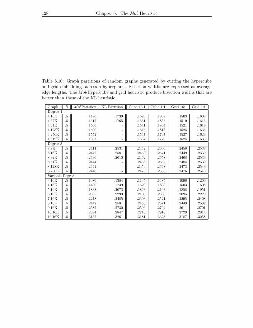
128 Chapter 6. The Mob Heuristic
Table 6.10: Graph partitions of random graphs generated by cutting the hypercubeand grid embeddings across a hyperplane. Bisection widths are expressed as averageedge lengths. The Mob hypercube and grid heuristic produce bisection widths that arebetter than those of the KL heuristic.
Graph R MobPartition KL Partition Cube 16:1 Cube 1:1 Grid 16:1 Grid 1:1
Degree 4
4.16K .5 .1480 .1739 .1520 .1808 .1503 .16084.32K .5 .1512 .1765 .1551 .1835 .1510 .16164.64K .5 .1500 - .1541 .1804 .1521 .16194.128K .5 .1500 - .1545 .1813 .1525 .16364.256K .5 .1552 - .1547 .1797 .1527 .16294.512K .5 .1503 - .1567 .1770 .1524 .1633
Degree 8
8.8K .5 .2411 .2531 .2442 .2660 .2456 .25398.16K .5 .2442 .2581 .2453 .2671 .2449 .25398.32K .5 .2436 .2610 .2462 .2658 .2468 .25398.64K .5 .2444 - .2458 .2652 .2484 .25398.128K .5 .2442 - .2459 .2648 .2473 .25438.256K .5 .2440 - .2478 .2650 .2476 .2543
Variable Degree
3.16K .5 .1080 .1384 .1135 .1485 .1096 .12004.16K .5 .1480 .1739 .1520 .1808 .1503 .16085.16K .5 .1838 .2073 .1863 .2103 .1858 .19516.16K .5 .2085 .2290 .2100 .2330 .2095 .22207.16K .5 .2278 .2485 .2303 .2521 .2295 .24088.16K .5 .2442 .2581 .2453 .2671 .2449 .25399.16K .5 .2585 .2730 .2596 .2794 .2611 .270110.16K .5 .2694 .2847 .2710 .2910 .2729 .281416.16K .5 .3155 .3261 .3181 .3323 .3187 .3258

6.3. The Mob Graph-Embedding Heuristic 129
Comparison to Simulated Annealing Chen et al.[28,29] evaluated the perfor-
mance of 1-to-1 hypercube-embedding heuristics. The graphs to be embedded were
random graphs, random geometric graphs, random trees, hypercubes, and hypercubes
with randomly added and deleted edges. All graphs had 128 vertices and were embed-
ded in a 7-dimensional hypercube. Among the algorithms tested, simulated annealing
with a move set limited to swapping vertex pairs along hypercube edges produced the
best solutions.
We obtained the ten random graphs used by Chen et al. and also generated ten
random graphs with our own generator. For each graph five runs were performed, and
results were averaged over these runs. Each run of Mob was limited by 8000 iterations,
and a schedule as described above was used. Chen et al. report that on ten random
graphs of average degree 7, a reduction of 58.1% over the cost of a random embedding
was achieved. We found that the average solution produced by Mob is 58.28% for Chen
et al.’s graphs and 58.17% for our own graphs. Thus Mob’s performance was about
equal to the performance of a tuned version of SA.
Our experiments on much larger graphs, shown in Table 6.6, indicate that the
Mob achieves a 51.7% reduction for degree-7 graphs, with very little variation between
individual runs. Thus, the difference between 58.1% and 51.7% may well be an artifact
of using very small graphs. It would be interesting to see how SA performs on larger
examples, unless excessive running time prohibits experiments.
6.3.4 Experimental Results for Geometric Graphs
We performed experiments on random geometric graphs, which have more structure
than random graphs. The cost ratio of minimum embedding to random embedding
tends to be much smaller than for random graphs. This makes it more desirable to
find a good embedding, but also suggests that a good embedding is harder for a local
search heuristic to find. A random geometric graph Gn,d with n vertices and average
degree d is generated by randomly selecting n points in the unit square [0, 1) × [0, 1).
These points are the vertices of Gn,d. The geometric graph Gn,d contains an edge if the
vertex pairs are a distance r or less apart, as measured by a distance metric. To obtain
graphs of degree d, the distance parameter r is set to the value rd. Figure 6.6(a) shows
a random geometric graph, and Figure 6.6(b) shows a grid embedding of this graph.
The following three metrics have been used in the literature:
(a) Manhattan metric r = |x1 − x2| + |y1 − y2|rd =
√
d/2n
(b) Euclidean metric r =√
|x1 − x2|2 + |y1 − y2|2rd =
√
d/πn
(c) Infinity metric r = max(|x1 − x2|, |y1 − y2|)rd =
√
d/4n
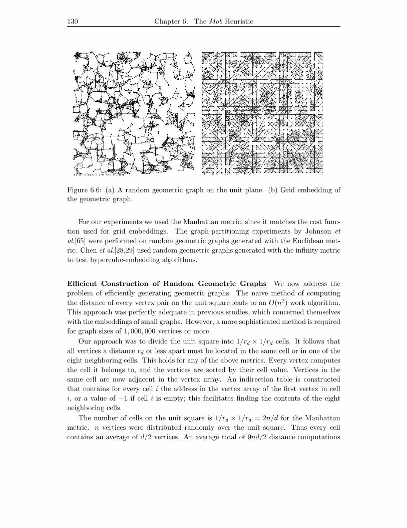
130 Chapter 6. The Mob Heuristic
Figure 6.6: (a) A random geometric graph on the unit plane. (b) Grid embedding ofthe geometric graph.
For our experiments we used the Manhattan metric, since it matches the cost func-
tion used for grid embeddings. The graph-partitioning experiments by Johnson et
al.[65] were performed on random geometric graphs generated with the Euclidean met-
ric. Chen et al.[28,29] used random geometric graphs generated with the infinity metric
to test hypercube-embedding algorithms.
Efficient Construction of Random Geometric Graphs We now address the
problem of efficiently generating geometric graphs. The naive method of computing
the distance of every vertex pair on the unit square leads to an O(n2) work algorithm.
This approach was perfectly adequate in previous studies, which concerned themselves
with the embeddings of small graphs. However, a more sophisticated method is required
for graph sizes of 1, 000, 000 vertices or more.
Our approach was to divide the unit square into 1/rd × 1/rd cells. It follows that
all vertices a distance rd or less apart must be located in the same cell or in one of the
eight neighboring cells. This holds for any of the above metrics. Every vertex computes
the cell it belongs to, and the vertices are sorted by their cell value. Vertices in the
same cell are now adjacent in the vertex array. An indirection table is constructed
that contains for every cell i the address in the vertex array of the first vertex in cell
i, or a value of −1 if cell i is empty; this facilitates finding the contents of the eight
neighboring cells.
The number of cells on the unit square is 1/rd × 1/rd = 2n/d for the Manhattan
metric. n vertices were distributed randomly over the unit square. Thus every cell
contains an average of d/2 vertices. An average total of 9nd/2 distance computations
6.3. The Mob Graph-Embedding Heuristic 131
is done to generate nd/2 edges, and the total computational work is O(n log n + nd).
Under the realistic assumption that sorting n vertices by their cell value takes time
O(log2n) with O(n) processors, the above algorithm is easily parallelized to run in
time O(log2 n+ d) with O(n) processors. Our experiments show that the constants are
very small.
Note that the above search structure works only for points distributed randomly
in the plane. More sophisticated algorithms, such as quad-trees, Voronoi diagrams,
and trapezoidal decompositions, have been developed in the field of computational
geometry to deal with nearest-neighbor problems. The considerable implementation
complexity and (usually) O(n log n) storage-space requirements make these algorithms
inappropriate for the special case of generating geometric graphs, since the much sim-
pler algorithm above exists.
We can derive a simple upper bound for the bisection width b of a geometric graph
Gn,d. Assume a vertical line divides the unit square into two sets containing n/2 vertices
each. We can place 1/rd cells along both sides of the line that contain an average of
d/2 vertices when the Manhattan metric is used. The edges Gn,d are of length rd or
less, so any edge that crosses the vertical line must have its two vertices in the cells
along the vertical line. A vertex in one cell can be connected by an edge to all vertices
in the three neighboring cells across the vertical line. Thus bmin, the average number
of edges crossing the vertical line, is
bmin ≤ 31
rd
(
d
2
)2
= 3√
n
(
d
2
)3/2
= O(√
n)
In a random graph partitioning of Gn,d half the edges cross the cut, so the average cost
br of a random graph partitioning is
br =nd
4
We estimate gmin, the minimum cost grid embedding, by superimposing a√
n × √n
grid on the unit square and assuming that the vertices of Gn,d are mapped to grid
vertices close to their locations on the unit square. Thus the total edge cost gmin under
the Manhattan metric is approximately
gmin ≈ nd
2rd
√n = n
(
d
2
)3/2
whereas gr, the average cost of a random embedding of Gn,d, can be estimated by
gr =nd
2
√n
Since we can fold the√
n × √n grid into a hypercube of dimension log n, the same
estimate as given above holds for hmin, the minimum cost hypercube embedding:
hmin ≈ nd
2rd
√n = n
(
d
2
)3/2
132 Chapter 6. The Mob Heuristic
whereas hr, the average cost of a random hypercube embedding of Gn,d can be estimated
by
hr =nd
4log n
The above estimates indicate that, for geometric graphs with increasing size, the ratio
of minimum-cost embeddings to random embeddings decreases asymptotically to 0.
The columns labeled Slice in Tables 6.12 and 6.13 show results for the Slice heuris-
tic, introduced below, that are close to the above estimates. (The results presented in
the tables are expressed as average edge lengths, and must be multiplied by the number
of edges nd/2 to give total embedding costs.)
The Slice Heuristic Intuitively, if every randomly generated vertex of Gn,d on the
unit square were shifted by a small distance so that the point occupied a unique grid
location, the resulting grid embedding should be quite good, and certainly better than
a randomly generated mapping of vertices to the grid. Such a heuristic can serve both
as a starting solution for the Mob heuristic and as a reference point to observe Mob’s
convergence from a random solution.
The Slice heuristic presented here is a divide-and-conquer algorithm to find unique
vertex to grid mappings by slightly displacing the vertices on the unit square. The
Slice heuristic is closely related to the slicing structure tree introduced by Otten[95] for
VLSI floorplan design. The vertices are sorted along the x- or the y-dimension. The
sorted vertices are divided into two sets, which are mapped to different halves of the
grid. Each set is now sorted along the other dimension. The procedure of sorting along
alternating dimensions and halving the vertex set and the grid node set is repeated until
the sets are of size one. At this point every vertex has a unique grid node assigned to
it.
Johnson et al.[65] used a similar approach in designing their LINE heuristic for par-
titioning geometric graphs: the unit square is cut into half to obtain a graph partition.
They report that local search algorithms do not converge quickly on geometric graphs,
local search algorithms need considerable running time to equal the performance of
LINE, and LINE followed by local search produced the best results.
Since x, y-coordinates are usually not part of the input to a graph-embedding prob-
lem, Slice is definitely not a practical graph-embedding heuristic. We present its results
here since we suspect it produces solutions very close to the optimal embedding; thus
allowing us to evaluate the performance of the Mob heuristic.
By itself, the knowledge that a graph G is a random geometric graph seems not to
be very helpful. A heuristic is required to construct approximate x- and y-coordinates
of G’s vertices in the unit square. Unfortunately, the best candidate for doing so is a
grid-embedding heuristic.
Experiments on Large Geometric Graphs We evaluated the performance of the
Mob hypercube and grid-embedding algorithms for geometric graphs with up to 256K
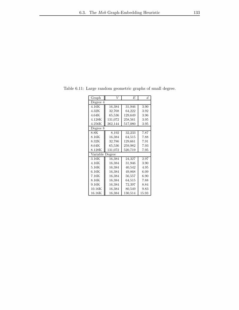
6.3. The Mob Graph-Embedding Heuristic 133
Table 6.11: Large random geometric graphs of small degree.
Graph V E d
Degree 4
4.16K 16,384 31,946 3.904.32K 32,768 64,222 3.924.64K 65,536 129,649 3.964.128K 131,072 258,561 3.954.256K 262,144 517,080 3.95
Degree 8
8.8K 8,192 32,233 7.878.16K 16,384 64,515 7.888.32K 32,786 129,661 7.918.64K 65,536 259,982 7.938.128K 131,072 520,719 7.95
Variable Degree
3.16K 16,384 24,327 2.974.16K 16,384 31,946 3.905.16K 16,384 40,542 4.956.16K 16,384 49,868 6.097.16K 16,384 56,557 6.908.16K 16,384 64,515 7.889.16K 16,384 72,397 8.8410.16K 16,384 80,549 9.8316.16K 16,384 130,514 15.93
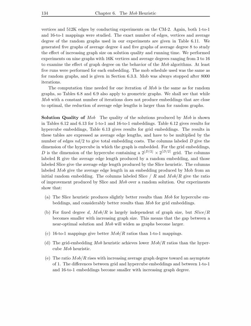
134 Chapter 6. The Mob Heuristic
vertices and 512K edges by conducting experiments on the CM-2. Again, both 1-to-1
and 16-to-1 mappings were studied. The exact number of edges, vertices and average
degree of the random graphs used in our experiments are given in Table 6.11. We
generated five graphs of average degree 4 and five graphs of average degree 8 to study
the effect of increasing graph size on solution quality and running time. We performed
experiments on nine graphs with 16K vertices and average degrees ranging from 3 to 16
to examine the effect of graph degree on the behavior of the Mob algorithms. At least
five runs were performed for each embedding. The mob schedule used was the same as
for random graphs, and is given in Section 6.3.3. Mob was always stopped after 8000
iterations.
The computation time needed for one iteration of Mob is the same as for random
graphs, so Tables 6.8 and 6.9 also apply to geometric graphs. We shall see that while
Mob with a constant number of iterations does not produce embeddings that are close
to optimal, the reduction of average edge lengths is larger than for random graphs.
Solution Quality of Mob The quality of the solutions produced by Mob is shown
in Tables 6.12 and 6.13 for 1-to-1 and 16-to-1 embeddings. Table 6.12 gives results for
hypercube embeddings, Table 6.13 gives results for grid embeddings. The results in
these tables are expressed as average edge lengths, and have to be multiplied by the
number of edges nd/2 to give total embedding costs. The columns labeled D give the
dimension of the hypercube in which the graph is embedded. For the grid embeddings,
D is the dimension of the hypercube containing a 2⌊D/2⌋ × 2⌈D/2⌉ grid. The columns
labeled R give the average edge length produced by a random embedding, and those
labeled Slice give the average edge length produced by the Slice heuristic. The columns
labeled Mob give the average edge length in an embedding produced by Mob from an
initial random embedding. The columns labeled Slice / R and Mob/R give the ratio
of improvement produced by Slice and Mob over a random solution. Our experiments
show that:
(a) The Slice heuristic produces slightly better results than Mob for hypercube em-
beddings, and considerably better results than Mob for grid embeddings.
(b) For fixed degree d, Mob/R is largely independent of graph size, but Slice/R
becomes smaller with increasing graph size. This means that the gap between a
near-optimal solution and Mob will widen as graphs become larger.
(c) 16-to-1 mappings give better Mob/R ratios than 1-to-1 mappings.
(d) The grid-embedding Mob heuristic achieves lower Mob/R ratios than the hyper-
cube Mob heuristic.
(e) The ratio Mob/R rises with increasing average graph degree toward an asymptote
of 1. The differences between grid and hypercube embeddings and between 1-to-1
and 16-to-1 embeddings become smaller with increasing graph degree.
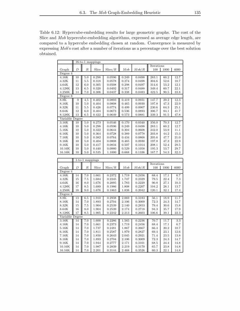
6.3. The Mob Graph-Embedding Heuristic 135
Table 6.12: Hypercube-embedding results for large geometric graphs. The cost of theSlice and Mob hypercube-embedding algorithms, expressed as average edge length, arecompared to a hypercube embedding chosen at random. Convergence is measured byexpressing Mob’s cost after a number of iterations as a percentage over the best solutionobtained.
16-to-1 mappingsIterations
Graph D R Slice Slice/R Mob Mob/R 100 1000 4000Degree 44.16K 10 5.0 0.298 0.0596 0.249 0.0498 283.1 60.2 12.74.32K 11 5.5 0.318 0.0578 0.274 0.0498 304.6 52.6 10.74.64K 12 6.0 0.305 0.0508 0.298 0.0497 314.6 53.2 12.14.128K 13 6.5 0.320 0.0492 0.317 0.0488 349.4 60.7 22.14.256K 14 7.0 0.306 0.0437 0.338 0.0483 422.5 90.5 33.8Degree 88.8K 9 4.5 0.402 0.0893 0.419 0.0931 147.7 29.2 12.38.16K 10 5.0 0.404 0.0808 0.465 0.0930 197.8 47.3 22.98.32K 11 5.5 0.426 0.0774 0.499 0.0907 230.6 64.3 25.18.64K 12 6.0 0.404 0.0673 0.536 0.0893 306.7 84.1 41.78.128K 13 6.5 0.422 0.0649 0.573 0.0881 339.3 91.5 47.8Variable Degree3.16K 10 5.0 0.273 0.0546 0.170 0.0340 356.0 70.3 12.74.16K 10 5.0 0.298 0.0596 0.249 0.0498 283.1 60.2 12.75.16K 10 5.0 0.322 0.0644 0.304 0.0608 242.0 53.9 11.16.16K 10 5.0 0.364 0.0728 0.389 0.0778 203.8 44.2 15.37.16K 10 5.0 0.382 0.0764 0.434 0.0868 205.6 47.7 21.08.16K 10 5.0 0.404 0.0808 0.465 0.0930 197.8 47.3 22.99.16K 10 5.0 0.417 0.0834 0.507 0.1014 208.1 52.4 29.510.16K 10 5.0 0.440 0.0880 0.529 0.1058 195.3 53.7 29.716.16K 10 5.0 0.535 1.1000 0.668 0.1336 167.7 54.3 32.3
1-to-1 mappingsIterations
Graph D R Slice Slice/R Mob Mob/R 100 1000 4000Degree 44.16K 14 7.0 1.661 0.2372 1.719 0.2456 68.4 17.1 6.74.32K 15 7.5 1.684 0.2245 1.747 0.2329 79.5 22.4 7.34.64K 16 8.0 1.676 0.2095 1.783 0.2229 90.8 27.1 10.34.128K 17 8.5 1.689 0.1986 1.808 0.2207 104.2 28.1 13.74.256K 18 9.0 1.676 0.1863 1.838 0.2042 120.1 32.1 17.4Degree 88.8K 13 6.5 1.910 0.2938 2.069 0.3183 56.1 18.9 11.78.16K 14 7.0 1.893 0.2704 2.106 0.3009 72.3 24.3 14.78.32K 15 7.5 1.904 0.2539 2.140 0.2853 79.4 30.6 15.88.64K 16 8.0 1.904 0.2539 2.174 0.2718 94.3 35.7 17.98.128K 17 8.5 1.905 0.2242 2.213 0.2603 106.6 39.1 22.3Variable Degree3.16K 14 7.0 1.600 0.2286 1.565 0.2236 70.7 11.7 3.34.16K 14 7.0 1.661 0.2373 1.719 0.2456 68.4 17.1 6.75.16K 14 7.0 1.737 0.2481 1.867 0.2667 66.4 20.2 10.76.16K 14 7.0 1.811 0.2587 1.979 0.2827 69.4 23.1 12.67.16K 14 7.0 1.850 0.2643 2.045 0.2921 71.4 23.5 13.88.16K 14 7.0 1.893 0.2704 2.106 0.3009 72.3 24.3 14.79.16K 14 7.0 1.944 0.2777 2.171 0.3101 68.5 24.4 14.810.16K 14 7.0 1.987 0.2839 2.219 0.3170 65.7 23.8 14.816.16K 14 7.0 2.201 0.3144 2.468 0.3526 60.3 22.1 14.8
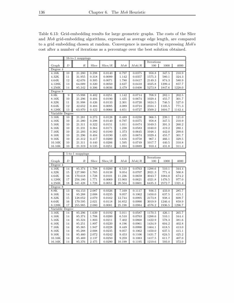
136 Chapter 6. The Mob Heuristic
Table 6.13: Grid-embedding results for large geometric graphs. The costs of the Sliceand Mob grid-embedding algorithms, expressed as average edge length, are comparedto a grid embedding chosen at random. Convergence is measured by expressing Mob’scost after a number of iterations as a percentage over the best solution obtained.
16-to-1 mappingsIterations
Graph D R Slice Slice/R Mob Mob/R 100 1000 4000Degree 44.16K 10 21.280 0.298 0.0140 0.797 0.0375 958.8 347.5 210.94.32K 11 31.955 0.318 0.0099 1.142 0.0357 1575.3 580.1 324.34.64K 12 42.676 0.305 0.0071 1.780 0.0417 2149.3 874.3 580.94.128K 13 64.009 0.320 0.0050 2.627 0.0410 3325.8 1299.4 857.74.256K 14 85.342 0.306 0.0036 3.479 0.0408 5273.8 1847.6 1228.0Degree 88.8K 9 15.998 0.402 0.0251 1.142 0.0714 708.9 282.1 202.58.16K 10 21.296 0.404 0.0190 1.435 0.0674 1029.4 455.7 301.78.32K 11 31.998 0.426 0.0133 2.301 0.0720 1624.5 746.5 527.08.64K 12 42.652 0.404 0.0095 3.089 0.0724 2334.1 1105.5 771.38.128K 13 63.970 0.422 0.0066 4.651 0.0727 3509.2 1604.7 1142.4Variable Degree3.16K 10 21.281 0.273 0.0128 0.489 0.0230 966.5 239.1 121.04.16K 10 21.280 0.298 0.0140 0.797 0.0375 958.8 347.5 210.95.16K 10 21.311 0.322 0.0151 1.011 0.0474 1049.5 391.3 260.26.16K 10 21.231 0.364 0.0171 1.238 0.0583 1040.0 419.2 280.17.16K 10 21.293 0.382 0.0180 1.373 0.0645 1048.1 442.0 299.68.16K 10 21.296 0.404 0.0190 1.435 0.0674 1029.4 455.7 301.79.16K 10 21.312 0.417 0.0200 1.616 0.0758 967.1 466.1 329.510.16K 10 21.311 0.440 0.0206 1.595 0.0749 1017.7 440.5 310.816.16K 10 21.319 0.535 0.0251 1.894 0.0889 910.4 431.8 311.4
1-to-1 mappingsIterations
Graph D R Slice Slice/R Mob Mob/R 100 1000 4000Degree 44.16K 14 85.374 1.708 0.0200 6.510 0.0763 1288.6 510.1 344.44.32K 15 127.980 1.765 0.0138 9.054 0.0707 2021.3 771.4 500.84.64K 16 170.618 1.728 0.0101 11.236 0.0659 3043.7 1084.0 674.24.128K 17 256.180 1.771 0.0069 15.903 0.0621 4321.8 1476.5 977.04.256K 18 341.428 1.728 0.0051 20.504 0.0601 6435.3 2572.7 1321.4Degree 88.8K 13 64.153 2.087 0.0326 7.169 0.1117 936.5 433.0 285.78.16K 14 85.288 2.008 0.0235 9.057 0.1062 1450.0 637.5 415.18.32K 15 128.052 2.079 0.0162 12.744 0.0995 2173.8 938.4 609.78.64K 16 170.595 2.021 0.0118 16.852 0.0990 3019.9 1246.4 859.98.128K 17 255.985 2.080 0.0081 25.198 0.0984 4576.2 1936.5 1296.7Variable Degree3.16K 14 85.296 1.639 0.0192 5.011 0.0587 1170.5 426.1 265.74.16K 14 85.374 1.708 0.0200 6.510 0.0763 1288.6 510.1 344.45.16K 14 85.324 1.803 0.0211 7.402 0.0868 1422.9 578.3 381.66.16K 14 85.251 1.897 0.0220 8.196 0.0961 1434.9 604.2 402.87.16K 14 85.365 1.947 0.0228 8.449 0.0990 1464.1 618.5 413.08.16K 14 85.288 2.008 0.0235 9.057 0.1062 1450.0 637.5 415.19.16K 14 85.460 2.072 0.0242 9.453 0.1106 1431.7 624.5 425.210.16K 14 85.469 2.137 0.0250 9.259 0.1083 1417.5 611.7 407.016.16K 14 85.376 2.475 0.0290 10.199 0.1195 1219.6 593.0 372.0
6.3. The Mob Graph-Embedding Heuristic 137
(f) The ratio Mob/R is smaller for geometric graphs than for random graphs. (Com-
pare Tables 6.6, 6.7 to Tables 6.12, 6.13). For 16-to-1 and 1-to-1 grid embeddings
and for 1-to-1 hypercube embeddings, Mob/R is almost ten times smaller for
degree-4 graphs, and almost five times smaller for degree-8 graphs. For 1-to-1
hypercube embeddings, the ratio Mob/R for geometric graphs is about half of
the ratio Mob/R for random graphs. So while Mob with a constant number of
iterations does not produce embeddings that are close to optimal, the reduction
of average edge lengths is larger than for random graphs.
Rates of Convergence of Mob Tables 6.12 and6.13 also report the convergence
of Mob for increasing iterations. The columns labeled Iterations show the average
embedding cost as percentages above the best-ever embedding cost, produced after 100,
1000 and 4000 iterations of Mob, respectively. Our experiments for geometric graphs
indicate that Mob still converges rapidly towards a solution that is good compared to
the best-ever solution produced by Mob. However, as can be inferred from the Iterations
columns, the cost ratio of a Mob solution divided by the best solution (produced by
Slice) increases with increasing graph size.
Comparison to Graph-partitioning Algorithms To calibrate our results, we
again measured the graph partitions produced by the hypercube and grid embeddings,
as described in Section 6.3.3. Table 6.14 shows how the Mob hypercube and grid
embedding algorithms behaved as graph-partitioning algorithms, compared to the Mob
graph-partitioning algorithm and the KL graph-partitioning algorithm.
The cost of the graph embeddings P = (X,Y ) is given in Table 6.14 as the per-
centage of all edges that cross the cut between X and Y . The Mob graph-partitioning
heuristic produced better results that the hypercube- and grid-embedding algorithms,
but does not approach the partitions produced by Slice. At least with a constant num-
ber of iterations, the Mob heuristics produce embeddings in which the average edge
length as a function of graph size is constant or decreases slowly, whereas the aver-
age edge lengths produced by Slice as a function of graph size decrease quickly, about
O(1/√
n).
We found that both 16-to-1 embedding algorithms and the grid 1-to-1 embedding
algorithm produced good graph partitions that were larger by a factor of roughly 1.5
to 4 than the Mob graph-partitioning algorithm. The KL graph-partitioning algo-
rithm, which we ran only on graphs with 32K (or fewer) vertices due to running-time
considerations, was slightly worse than these three graph-embedding heuristics. The
hypercube 1-to-1 algorithm produced graph partitions that were roughly larger by an
order of magnitude.
As for random graphs, we find the performance of the Mob embedding algorithms
used as graph-partitioning algorithms remarkable, considering that Mob is optimizing
the “wrong” cost function. None of the local search algorithms we implemented was
able to get close to the results produced by Slice.

138 Chapter 6. The Mob Heuristic
Table 6.14: Graph partitions of geometric graphs generated by cutting the hypercubeand grid embeddings across a hyperplane. Bisection widths are expressed as averageedge lengths. The Mob hypercube and grid heuristic produce bisection widths compa-rable to those of the Mob graph-partitioning heuristic and better than those of the KLheuristic.
Graph R Slice Mob Partition KL Partition Cube 16:1 Cube 1:1 Grid 16:1 Grid 1:1
Degree 4
4.16K .5 0.0031 0.0093 0.0376 0.0230 0.1174 0.0166 0.02914.32K .5 0.0027 0.0130 0.0421 0.0238 0.1081 0.0156 0.02844.64K .5 0.0014 0.0143 0.0409 0.0235 0.1053 0.0186 0.02664.128K .5 0.0015 0.0146 - 0.0238 0.1004 0.0185 0.02574.256K .5 0.0009 0.0116 - 0.0236 0.0974 0.0188 0.0243
Degree 8
8.8K .5 0.0066 0.0204 0.0438 0.0422 0.1472 0.0300 0.04208.16K .5 0.0047 0.0177 0.0476 0.0433 0.1423 0.0284 0.04228.32K .5 0.0037 0.0171 0.0463 0.0431 0.1382 0.0300 0.03908.64K .5 0.0026 0.0228 - 0.0431 0.1296 0.0297 0.04018.128K .5 0.0016 0.0196 - 0.0428 0.1250 0.0322 0.0413
Variable Degree
3.16K .5 0.0022 0.0077 0.0293 0.0146 0.1028 0.0091 0.02254.16K .5 0.0031 0.0093 0.0376 0.0230 0.1174 0.0166 0.02915.16K .5 0.0033 0.0162 0.0464 0.0288 0.1253 0.0203 0.03396.16K .5 0.0050 0.0139 0.0496 0.0365 0.1304 0.0257 0.03867.16K .5 0.0049 0.0154 0.0565 0.0414 0.1360 0.0248 0.04238.16K .5 0.0047 0.0177 0.0476 0.0433 0.1423 0.0275 0.04079.16K .5 0.0042 0.0103 0.0517 0.0459 0.1441 0.0284 0.042210.16K .5 0.0059 0.0213 0.0477 0.0483 0.1502 0.0320 0.044516.16K .5 0.0072 0.0175 0.0542 0.0579 0.1597 0.0335 0.0480
Table 6.15: Hypercube embeddings of 128-vertex, degree-7 geometric graphs. Compar-ison of Mob to SA.
Heuristic Min Avg. Cost Avg. Edge Length % of Random
Mob + Slice 620 676.0 1.694 47.7Mob 649 702.7 1.758 49.5Slice 664 737.6 1.849 52.1Random 1320 1410.1 3.552 100.0
SAC (pushed) 694 742.8 1.691 48.0

6.3. The Mob Graph-Embedding Heuristic 139
Comparison to Simulated Annealing Analogously to the experiments with ran-
dom graphs, we compared the performance of the Mob cube-embedding heuristic on
geometric graphs to the results reported for simulated annealing by Chen et al.[28,29].
To duplicate their experiments, we generated 10 random geometric graphs with our
own generator. Each graph had 128 vertices. The distance parameter for the infinity
metric was set to rd =√
d/4n = 0.117386 to obtain graphs of degree 7.
For each graph five runs were performed and results were averaged over these runs.
Each run of Mob was limited by 8000 iterations, and a schedule as described above
was used. The results, expressed as percent reduction in edge lengths of a random
embedding, are given in Table 6.15. Chen et al. report that on ten random geometric
graphs of average degree 7, a reduction of 48.0% was achieved by SAC, a version of SA
with the move set limited to hypercube edges. We found that the average reduction
produced by Mob is 49.5% for our own graphs. The Slice heuristic produced solutions
with 52.1% reductions. The best solutions were obtained when the solutions produced
by Slice were further improved by Mob.


141
Chapter 7
Conclusions and Open Problems
We believe that eventually the entire suite of CAD tools used to design VLSI chips,
from high-level specification to the generation of masks for fabrication, will run on a
massively parallel machine. There are various reasons for eliminating all serial elements
from the system: a CAD system designed for a homogeneous underlying machine ar-
chitecture is more elegant and reduces code complexity, serial tools would limit the
overall speed of the CAD system, and the process of transferring intermediate design
representations back and forth between serial and parallel machines would introduce
serial bottlenecks.
We have concentrated here on problems related to parallel layout synthesis. There
are other areas in VLSI CAD in which parallelism can reduce design time by several
orders of magnitude and can allow the creation of new tools to handle larger problem in-
stances and return higher-quality solutions. The most active research area is currently
parallel simulation at all levels, including high-level behavioral simulation, switch-level
simulation, logic simulation, and semiconductor device modeling. The problems of
test-vector generation, database access and management, and parsing languages for
intermediate design representations are all promising candidates for research in par-
allelism. (See the excellent surveys by Preas and Lorenzetti[99] and Lengauer[85] for
detailed problem descriptions and further references.)
Channel Routing
We have demonstrated in Chapter 3 that massive parallelism is inherent in channel
routing. Our parallel channel-routing algorithm for channels without column conflicts
is in NC1(n/ log n). The constants hidden in the O() notation are very small. The
algorithm and its extensions are composed of simple primitives that can be tuned to run
very fast on an actual multiple-processor machine. This algorithm is directly related to
the coloring of an interval graph and is based on the left-edge heuristic of Hashimoto
and Stevens[58]. It can be applied as a subroutine in other channel routers based on
the left-edge heuristic.
142 Chapter 7. Conclusions and Open Problems
The extensions to the basic channel-routing algorithm that developed to deal with
column conflicts need to be examined for parallelism. We have shown in Chapter 5 that
any local search heuristic that minimizes the number of column conflicts in a channel
routing by accepting cost-improving swaps of tracks or subtracks is P-hard. It would
be interesting to know whether Fiduccia and Rivest’s greedy channel router [105] and
YACR2 by Reed et al.[102] are hard to parallelize.
Compaction
We have given a parallel algorithm for computing the transitive reduction of an interval
dag. This is equivalent to a parallel algorithm for computing a minimum-distance
constraint dag from a VLSI layout, and is substantially simpler than a previously
published serial algorithm. An intermediate result during the execution of the above
algorithm is a parallel algorithm to construct a tiling or corner stitching, a geometrical
data structure used in the Magic VLSI layout system. All these computations take
time O(log2 n) using O(n/log n) processors on an EREW PRAM, so their processor-
time product is optimal. We designed our algorithm to use local operations plus the
parallel primitives sort, merge and parallel prefix. We implemented a prototype of the
compaction algorithm on the CM-2 Connection Machine, and found that the time to
construct the horizontal visibility graph of a 128K-rectangle layout is ≈ 20 seconds
using 16K processors.
Further research is needed to obtain efficient parallel shortest-path algorithms for
general, planar or VLSI-specific graphs. The constraint-graph model must be aug-
mented to deal with issues that arise in practice, such as the addition of equality
constraints (two units must touch) and upper-bound constraints (two units should not
be too far apart). Also, in practice VLSI layouts are modeled by multiple layers of
rectangles and these layers must be coordinated. Such a system must also incorporate
a mechanism for stretching and jogging wires. All of these issues must be examined
from the point of view of parallelism.
The Parallel Complexity of Local Search
We have shown in Chapter 5 that the Kernighan-Lin graph-partitioning heuristic is P-
complete. We have also shown that the zero-temperature version of simulated annealing
is P-hard. Thus, it is unlikely that either heuristic can be parallelized. We have seen
that certain local search heuristics based on the SWAP neighborhood, such as simulated
annealing for cube-embedding and grid-embedding problems, are P-hard. This suggests
that there is (probably) no parallel SA algorithm that does exactly what the serial
algorithm does.
We believe that many other P-complete or P-hard local search heuristics for NP-
complete problems can be found. In the area of VLSI placement, grid-embedding
heuristics are used with cost functions that measure wiring congestion and maximum
143
wire lengths. The equivalent cost functions for hypercube embedding measure rout-
ing congestion and maximum routing-path length. Local search heuristics for these
important graph-embedding problems need to be examined for P-hardness.
The MobHeuristic
In Chapter 6 we presented a new massively parallel heuristic, the Mob heuristic, that
is closely related to both Kernighan-Lin and simulated annealing. We applied our
heuristic to the graph-partitioning, grid and hypercube-embedding problems, which
are closely related to VLSI placement. We ran Mob on the CM-2 to show that it
is massively parallel, is fast and can handle very large graphs. The speed of the Mob
heuristic should be adequate for the optimized placement of large (100,000 to 1,000,000
gates) circuits.
Mob can be applied to other optimization problems in which local search heuristics
have been successful. It would be interesting to see the Mob heuristic used in an indus-
trial production system for VLSI gate-array placement or full custom logic placement.
Mob’s speed and its ability to handle unusually large problem sizes could reduce design
time by several orders of magnitude and would allow the creation of new tools to handle
larger problem instances and return higher-quality solutions. We plan to apply Mob to
the traveling salesman problem, the best known and most widely researched benchmark
problem for optimization heuristics, for further comparisons with simulated annealing
and other standard algorithms.

Bibliography 145
Bibliography
[1] “Connection Machine Model CM-2 Technical Summary,” Thinking Machines Cor-
poration TMC Technical Report HA 87-4, 1987.
[2] F. Afrati, C. H. Papadimitriouand G. Papadimitriou, “The Complexity of Cubical
Graphs,” in Information and Control, pp. 53–60, 1985.
[3] M. Ajtai, J. Komlosand E. Szemeredi, “An O(n log n) Sorting Network,” in 15th
Annual ACM Symposium on Theory of Computing, pp. 1–9, 1983.
[4] A. Apostolico, M. J. Atallah, L. L. Larmoreand H. S. McFaddin, “Efficient Parallel
Algorithms for String Editing and Related Problems,” preprint, Feb. 1988.
[5] M. J. Atallah, R. Coleand M. T. Goodrich, “Cascading Divide-and-Conquer: A Tech-
nique for Designing Parallel Algorithms,” in 28th Annual Symposium on Foundations
of Computer Science, pp. 151–160, 1987.
[6] P. Banerjee, M. H. Jonesand J. S. Sargent, “Parallel Simulated Annealing Algorithms
for Cell Placement on Hypercube Multiprocessors,” IEEE Transactions on Parallel
and Distributed Systems, vol. PDS-1, no. 1, pp. 91–106, January 1990.
[7] K. E. Batcherand H. S. Stone, “Sorting Networks and Their Applications,” AFIPS
Proc., Spring Joint Comput. Conf., vol. 32, pp. 307–314, 1968.
[8] M. Ben-Or, “Lower Bounds for Algebraic Computation Trees,” in 15th Annual ACM
Symposium on Theory of Computing, pp. 80–86, May 1983.
[9] S. Bettayeb, Z. Millerand I. H. Sudborough, “Embedding Grids into Hypercubes,” in
VLSI Algorithms and Architectures: 3rd Aegean Workshop on Computing, pp. 201–
211, 1988.
[10] G. Bilardiand A. Nicolau, “Bitonic Sorting with O(N log N) comparisons,” in 20th
Annual Conf. on Inform. Sci. and Systems, Princeton University, Princeton, NJ,
1986.
[11] G. Bilardiand A. Nicolau, “Adaptive Bitonic Sorting: An Optimal Parallel Algorithm
for Shared-Memory Machines,” SIAM Journal on Computing, vol. 18, no. 2, pp. 216–
228, Apr. 1989.
[12] G. Blelloch, “Scans as Primitive Parallel Operations,” in Proc. 1987 International
Conference on Parallel Processing, pp. 355–362, 1987.
146 Bibliography
[13] G. E. Blelloch, “Scans as Primitive Parallel Operations,” IEEE Transactions on
Computers, vol. 38, no. 11, pp. 1526–1538, 1989.
[14] S. H. Bokhari, “On the Mapping Problem,” IEEE Transactions on Computers, vol.
C-30, no. 3, pp. 207–214, Mar. 1981.
[15] S. W. Bollingerand S. F. Midkiff, “Processor and Link Assignment in Multicomput-
ers Using Simulated Annealing,” Proceedings International Conference on Parallel
Processing, vol. 1, pp. 1–6, 1988.
[16] A. Borodinand J. E. Hopcroft, “Routing, Merging, and Sorting on Parallel Models
of Computation,” J. Comp. Sys. Sci, vol. 30, pp. 130–145, 1985.
[17] G. J. Brebnerand L. G. Valiant, “Universal Schemes for Parallel Computation,” in
13th Annual ACM Symposium on Theory of Computing, pp. 263–277, 1981.
[18] M. A. Breuer, “Min-Cut Placement,” Design Automation and Fault-Tolerant Com-
puting, vol. 1, no. 4, pp. 343–362, Aug. 1977.
[19] R. J. Brouwerand P. Banerjee, “A Parallel Simulated Annealing Algorithm for Chan-
nel Routing on a Hypercube Multiprocessor,” in Proceedings of the International
Conference on Computer Design, pp. 4–7, 1988.
[20] T. Bui, S. Chaudhuri, F. T. Leightonand M. Sipser, “Graph Bisection Algorithms
with Good Average Case Behavior,” in 25th Annual Symposium on Foundations of
Computer Science, pp. 181–192, 1984.
[21] T. Bui, S. Chaudhuri, F. T. Leightonand M. Sipser, “Graph Bisection Algorithms
with Good Average Case Behavior,” Combinatorica, vol. 7, no. 3, pp. 171–191, 1987.
[22] T. Bui, C. Heigham, C. Jonesand T. Leighton, “Improving the Performance of the
Kernighan-Lin and Simulated Annealing Graph Bisection Algorithms,” in 26th IEEE
Design Automation Conference, pp. 775–778, 1989.
[23] T. N. Bui, “On Bisecting Random Graphs,” Dept. of Electrical Engineering and
Computer Science, M.I.T., MS Thesis MIT/LCS/TR-287, Feb. 1983.
[24] J. L. Burnsand A. R. Newton, “SPARCS: A New Constraint-Based IC Symbolic
Layout Spacer,” in Trans. IEEE Custom Integrated Circuits Conf., pp. 534–539,
May 1986.
[25] A. Casottoand A. Sangiovanni-Vincentelli, “Placement of Standard Cells Using Sim-
ulated Annealing on the Connection Machine,” in ICCAD, pp. 350–453, Nov. 1987.
[26] R. D. Chamberlain, M. N. Edelman, M. A. Franklinand E. E. Witte, “Simulated
Annealing on a Multiprocessor,” in Proceedings of the International Conference on
Computer Design, pp. 540–544, 1988.
[27] M. -Y. Chan, “Dilation-2 Embeddings of Grids into Hypercubes,” Proceedings In-
ternational Conference on Parallel Processing, vol. 3, pp. 295–298, 1988.
Bibliography 147
[28] W. -K. Chen, E. F. Gehringerand M. F. M. Stallmann, “Hypercube Embedding
Heuristics: An Evaluation,” International Journal of Parallel Programming, vol. 18,
no. 6, pp. 505–549, 1989.
[29] W. -K. Chenand M. F. M. Stallmann, “Local Search Variants for Hypercube Embed-
ding,” in Proceedings 5th Distributed Memory Computer Conference, pp. 1375–1383,
1990.
[30] Y. E. Cho, “A Subjective Review of Compaction,” in Proc. 22nd IEEE Design Au-
tomation Conference, pp. 396–404, 1985.
[31] R. Cole, “Parallel Merge Sort,” in 27th Annual Symposium on Foundations of Com-
puter Science, pp. 511–616, 1986.
[32] S. A. Cook, “The Complexity of Theorem-proving Procedures,” in 3rd Annual ACM
Symposium on Theory of Computing, pp. 151–158, 1971.
[33] S. A. Cook, “A Taxonomy of Problems with Fast Parallel Algorithms,” in Informa-
tion and Control, pp. 2–22, 1985.
[34] C. Corneiland R. C. Read, “The Graph Isomorphism Disease,” Journal of Graph
Theory , vol. 1, no. 4, pp. 339–363, 1977.
[35] E. D. Dahl, “Mapping and Compiled Communication on the Connection Machine,”
in Proceedings 5th Distributed Memory Computer Conference, pp. 756–766, 1990.
[36] B. A. Dalio, “DeCo–A Hierarchical Device Compilation System,” Dept. of Computer
Science, Brown University, PhD Thesis CS-87-08, May 1987and B. A. Dalio.
[37] B. A. Dalioand J. E. Savage, “DeCo–A Device Compilation System,” in International
Workshop on Logic and Architecture Synthesis for Silicon Compilers, May 1988.
[38] F. Darema, S. Kirkpatrickand V. A. Norton, “Parallel Algorithms for Chip Place-
ment by Simulated Annealing,” IBM Journal of Research and Development, vol. 31,
no. 3, pp. 391–401, May 1987.
[39] D. N. Deutsch, “A Dogleg Channel Router,” in Proc. 13th IEEE Design Automation
Conference, pp. 425–433, 1976.
[40] D. N. Deutsch, “Compacted Channel Routing,” in Proc. of the IEEE Intl. Conf. on
Computer-Aided Design, ICCAD-85, pp. 223–225, 1985.
[41] D. Dobkinand R. Lipton, “On the Complexity of Computations Under Varying Sets
of Primitives,” Journal of Computer and Systems Sciences, vol. 18, pp. 86–91, 1979.
[42] J. Doenhardtand T. Lengauer, “Algorithmic Aspects of One-Dimensional Layout
Compaction,” IEEE Transactions on Computer-Aided Design, vol. CAD-6, no. 5,
pp. 863–878, Sept. 1987.
[43] D. Dolev, K. Karplus, A. Siegel, A. Strongand J. D. Ullman, “Optimal Wiring be-
tween Rectangles,” in 13th Annual ACM Symposium on Theory of Computing,
pp. 312–317, 1981.
148 Bibliography
[44] A. E. Dunlopand B. W. Kernighan, “A Procedure for Placement of Standard-Cell
VLSI Circuits,” IEEE Transactions on Computer-Aided Design, vol. CAD-4, no. 1,
pp. 92–98, Jan. 1985.
[45] H. Edelsbrunner, M. H. Overmarsand D. Wood, “Graphics in Flatland,” Advances
in Computing Research, vol. 1, pp. 35–59, 1983.
[46] F. E. Fich, “New Bounds for Parallel Prefix Circuits,” in 15th Annual ACM Sym-
posium on Theory of Computing, pp. 27–36, 1983.
[47] C. M. Fiducciaand R. M. Mattheyses, “A Linear-Time Heuristic for Improving Net-
work Partitions,” in 19th IEEE Design Automation Conference, pp. 175–181, 1982.
[48] K. Fukunaga, S. Yamadaand T. Kasai, “Assignment of Job Modules onto Array
Processors,” IEEE Transactions on Computers, vol. c-36, no. 7, pp. 888–891, July
1987 .
[49] M. R. Gareyand D. S. Johnson, Computers and Intractability: A Guide to the Theory
of NP-Completeness. Freeman, New York, 1979.
[50] S. Gemanand D. Geman, “Stochastic Relaxation, Gibbs Distributions, and the Bayesian
Restoration of Images,” in Neurocomputing: Foundations of Research, J. A. Ander-
sonand E. Rosenfeld, Eds. MIT Press, 1988.
[51] J. Gill, “Computational Complexity of Probabilistic Turing Machines,” SIAM Jour-
nal on Computing, vol. 6, no. 4, pp. 675–695, 1977.
[52] L. M. Goldschlager, “The Monotone and Planar Circuit Value Problems,” ACM
Sigact News, vol. 9, no. 2, pp. 25–29, 1977.
[53] L. M. Goldschlager, “A Space Efficient Algorithm for the Monotone Planar Circuit
Value Problem,” Information Processing Letters, vol. 10, no. 1, pp. 25–27, 1980.
[54] M. Golumbic, Algorithmic Graph Theory and Perfect Graphs. Academic Press,
New York, 1980.
[55] D. R. Greening, “A Taxonomy of Parallel Simulated Annealing Techniques,” IBM,
Technical Report No. RC 14884, 1989.
[56] F. Harary, Graph Theory. Addison-Wesley, Reading, MA, 1969.
[57] B. Harperand J. H. Haynes, Jaguar E Type Owners Workshop Manual. Haynes
Publishing Group, 1974.
[58] A. Hashimotoand J. Stevens, “Wire Routing by Optimizing Channel Assignments
Within Large Apertures,” in Proc. 6th IEEE Design Automation Conference, pp. 155–
163, 1971.
[59] D. V. Heinbuch, CMOS3 Cell Library. Addison-Wesley, Reading, MA, 1988.
[60] D. Helmboldand E. Mayr, “Two-Processor Scheduling is in NC,” in VLSI Algorithms
and Architectures: 2nd Aegean Workshop on Computing , pp. 12–25, 1986.
[61] W. D. Hillis, The Connection Machine. MIT Press, 1985.
Bibliography 149
[62] D. S. Hirschberg, A. K. Chandraand D. V. Sarvate, “Computing Connected Com-
ponents on a Parallel Computer,” CACM , vol. 22, pp. 461–464, 1979.
[63] C. -T. Hoand S. L. Johnsson, “On the Embedding of Arbitrary Meshes in Boolean
Cubes with Expansion Two Dilation Two,” in Proceedings International Conference
on Parallel Processing, pp. 188–191, 1987.
[64] K. E. Iverson, A Programming Language. Wiley, New York, 1962.
[65] D. S. Johnson, C. A. Aragon, L. A. McGeochand C. Schevon, “Optimization by
Simulated Annealing: An Experimental Evaluation (Part 1),” Operations Research,
vol. 37, no. 6, pp. 865–892, Nov.-Dec. 1989.
[66] D. S. Johnson, C. H. Papadimitriouand M. Yannakakis, “How Easy is Local Search?,”
in Journal of Computer and Systems Sciences, pp. 79–100, 1988.
[67] R. M. Karpand V. Ramachandran, “A Survey of Parallel Algorithms for Shared-
Memory Machines,” in Handbook of Theoretical Computer Science. North-Holland,
1988.
[68] B. W. Kernighanand S. Lin, “An Efficient Heuristic Procedure for Partitioning
Graphs,” AT&T Bell Labs. Tech. J., vol. 49, pp. 291–307, Feb. 1970.
[69] S. Kirkpatrick, C. D. Gelattand M. P. Vecchi, “Optimization by Simulated Anneal-
ing,” Science, vol. 220, no. 4598, pp. 671–680, May 1983.
[70] P. N. Klein, “Efficient Parallel Algorithms for Chordal Graphs,” in 29th Annual
Symposium on Foundations of Computer Science, pp. 150–161, 1988.
[71] S. Kravitzand R. Rutenbar, “Multiprocessor-based Placement by Simulated Anneal-
ing,” in 23rd IEEE Design Automation Conference, pp. 567–573, 1986.
[72] B. Krishnamurthy, “An Improved Min-Cut Algorithm for Partitioning VLSI Net-
works,” IEEE Trans. Computers, vol. 33, no. 5, pp. 438–446, May 1984.
[73] E. S. Kuhand T. Yoshimura, “Efficient Algorithms for Channel Routing,” IEEE
Transactions on Computer-Aided Design, vol. CAD-1, no. 1, pp. 25–35, Jan. 1982.
[74] A. S. LaPaugh, “Algorithms for Integrated Circuit Layout: an Analytic Approach,”
Dept. of Electrical Engineering and Computer Science, M.I.T., PhD Thesis, 1980.
[75] R. E. Ladner, “The Circuit Value Problem is Log Space Complete for P,” ACM
SIGACT News, vol. 7, no. 1, pp. 18–20, 1975.
[76] R. E. Ladnerand M. J. Fischer, “Parallel Prefix Computation,” Journal of the ACM ,
vol. 27, pp. 831–838, 1980.
[77] J. Lamand J. -M. Delosme, “Simulated Annealing: a Fast Heuristic for Some Generic
Layout Problems,” in ICCAD, pp. 510–513, 1988.
[78] F. T. Leighton, Introduduction to Parallel Algorithms & and Architectures. Mor-
gan Kaufmann Publishers, San Mateo, 1991.
[79] F. T. Leighton, “A Layout Strategy for VLSI Which is Provably Good,” in 14th
Annual ACM Symposium on Theory of Computing, pp. 85–98, May 1982.
150 Bibliography
[80] T. Leighton, “Tight Bounds on the Complexity of Parallel Sorting,” IEEE Transac-
tions on Computers, vol. C-34, pp. 344–354, 1985.
[81] T. Leighton, C. E. Leiserson, B. Maggs, S. Plotkinand J. Wein, “Advanced Parallel
and VLSI Computation,” Dept. of Electrical Engineering and Computer Science,
M.I.T., MIT/LCS/RSS 2, Mar. 1988.
[82] T. Leighton, C. E. Leiserson, B. Maggs, S. Plotkinand J. Wein, “Theory of Parallel
and VLSI Computation,” Dept. of Electrical Engineering and Computer Science,
M.I.T., MIT/LCS/RSS 1, Mar. 1988.
[83] C. E. Leiserson, “VLSI Theory and Parallel Supercomputing,” in Advanced Research
in VLSI: Proceedings of the 1989 Decennial Caltech Conference , Cambridge, MA,
pp. 5–16, Mar. 1989.
[84] C. E. Leiserson, “Area-Efficient Graph Layouts (for VLSI),” in 21th Annual Sym-
posium on Foundations of Computer Science, pp. 270–281, Oct. 1980.
[85] T. Lengauer, Combinatorial Algorithms for Integrated Circuit Layout. John Wiley
& Sons, 1990.
[86] E. Lodiand L. Pagli, “A VLSI Algorithm for a Visibility Problem,” in International
Workshop on Parallel Computing and VLSI, pp. 125–134, 1984.
[87] M. Lundyand A. Mees, “Convergence of an Annealing Algorithm,” Mathematical
Programming, vol. 34, no. 1, pp. 111–124, 1986.
[88] M. A. Mahhowaldand C. Mead, “The Silicon Retina,” in Scientific American, pp. 76–
82, May 1991.
[89] K. Mehlhorn, Data Structures and Algorithms 1: Sorting and Searching. Springer-
Verlag, 1984.
[90] N. Metropolis, A. W. Rosenbluth, M. N. Rosenbluth, A. H. Tellerand E. Teller,
“Equations of State Calculations by Fast Computing Machines,” Journal of Chemical
Physics, vol. 6, no. 21, pp. 1087–1091, June 1953.
[91] D. Mitra, F. Romeoand A. Sangiovanni-Vincentelli, “Convergence and Finite-Time
Behaviour of Simulated Annealing,” Advances in Applied Probability , vol. 18, no.
3, pp. 747–771, Sept. 1986.
[92] B. Monienand I. H. Sudborough, “Simulating Binary Trees on Hypercubes,” in VLSI
Algorithms and Architectures: 3rd Aegean Workshop on Computing , pp. 170–180,
1988.
[93] R. C. Mosteller, A. H. Freyand R. Suaya, “2-D Compaction: A Monte Carlo Method,”
in Proc. Conference on Advanced Research in VLSI, pp. 173–197, 1987.
[94] K. Mulmuley, U. V. Vaziraniand V. V. Vazirani, “Matching is as Easy as Matrix
Inversion,” in 19th Annual ACM Symposium on Theory of Computing, pp. 345–354,
1987.
Bibliography 151
[95] R. H. J. M. Otten, “Automatic Floorplan Design,” in Proc. 19th IEEE Design Au-
tomation Conference, pp. 261–267, 1982.
[96] J. K. Ousterhout, “Corner Stitching: A Data-Structuring Technique for VLSI Layout
Tools,” IEEE Transactions on Computer-Aided Design, vol. CAD-3, no. 1, pp. 87–
100, Jan. 1984.
[97] N. Pippenger, “On Simultaneous Resource Bounds,” in 20th Annual Symposium on
Foundations of Computer Science, pp. 307–311, Oct. 1979.
[98] B. T. Preasand P. G. Karger, “Placement, Assignment and Floorplanning,” in Phys-
ical Design Automation of VLSI Systems, B. Preasand M. Lorenzetti, Eds. The
Benjamin/Cummings Publishing Company, Menlo Park, pp. 87–155, 1988.
[99] B. T. Preasand M. Lorenzetti, Eds., Physical Design Automation of VLSI Systems:
The Benjamin/Cummings Publishing Company, Menlo Park, 1988.
[100] F. P. Preparataand M. I. Shamos, Computational Geometry. Springer-Verlag, New
York, 1985.
[101] A. G. Ranade, “How to Emulate Shared Memory,” in 28th Annual Symposium on
Foundations of Computer Science, pp. 185–194, 1987.
[102] J. Reed, A. Sangiovanni-Vincentelliand M. Santomauro, “A New Symbolic Channel
Router: YACR2,” IEEE Transactions on Computer-Aided Design, vol. CAD-4, no.
3, pp. 208–219, July 1985.
[103] J. H. Reif, Ed., Synthesis of Parallel Algorithms: Morgan Kaufmann Publishers, San
Mateo, 1991.
[104] S. P. Reissand J. E. Savage, “SLAP–A Methodology for Silicon Layout,” in Procs.
Intl. Conf. on Circuits and Computers, pp. 281–285, 1982.
[105] R. L. Rivestand C. M. Fiduccia, “A Greedy Channel Router,” in Proc. 19th IEEE
Design Automation Conference, pp. 418–424, 1982.
[106] A. L. Rosenberg, Three-dimensional Integrated Circuitry. Computer Science Press,
1981.
[107] P. Roussel-Ragotand G. Dreyfus, “A Problem Independent Parallel Implementation
of Simulated Annealing: Models and Experiments,” IEEE Transactions on Computer-
Aided Design, vol. 9, no. 8, pp. 827–835, Aug. 1990.
[108] P. Sadayappanand F. Ercal, “Nearest-Neighbor Mapping of Finite Element Graphs
onto Processor Meshes,” IEEE Transactions on Computers, vol. C-36, no. 12, pp. 1408–
1424, Dec. 1987.
[109] P. Sadayappanand F. Ercal, “Cluster-Partitioning Approaches to Mapping Paral-
lel Programs onto a Hypercube,” in Supercomputing: 1st International Conference,
pp. 475–497, June 1987.
152 Bibliography
[110] M. Sarrafzadeh, “Channel-Routing Problem in the Knock-Knee Mode is NP-Complete,”
IEEE Transactions on Computer-Aided Design, vol. CAD-6, no. 4, pp. 503–506, July
1987.
[111] S. Sastryand A. Parker, “The Complexity of Two-Dimensional Compaction of VLSI
Layouts,” in Proc. Intl. Conf. on Circuits and Computers, pp. 402–406, Sept. 1982.
[112] C. Savage, “Parallel Algorithms for Graph Theoretic Problems,” Department of
Mathematics, Univ. of Illinois, PhD Thesis, 1977.
[113] J. E. Savage, The Complexity of Computing. John Wiley and Sons, 1976.
[114] J. E. Savage, “Planar Circuit Complexity and the Performance of VLSI Algorithms,”
in VLSI Systems and Computations, H. T. Kung, B. Sproulland G. Steele, Eds.
Computer Science Press, pp. 61–68, 1981.
[115] J. E. Savage, “Heuristics in the SLAP Layout System,” in IEEE Intl. Conf. On
Computer Design, Rye, New York, pp. 637–640, 1983.
[116] J. E. Savage, “Three VLSI Compilation Techniques: PLA’s, Weinberger Arrays, and
SLAP, A New Silicon Layout Program,” in Algorithmically-specialized Computers.
Academic Press, 1983.
[117] J. E. Savage, “Heuristics for Level Graph Embeddings,” in 9th International Work-
shop on Graph-Theoretic Concepts in Computer Science, pp. 307–318, June 1983.
[118] J. E. Savage, “The Performance of Multilective VLSI Algorithms,” Journal of Com-
puter and Systems Sciences, vol. 29, no. 2, pp. 243–273, Oct. 1984.
[119] J. E. Savageand M. G. Wloka, “Parallel Graph-Embedding and the Mob Heuristic,”
to be submitted, 1991.
[120] J. E. Savageand M. G. Wloka, “Parallelism in Graph Partitioning,” in Journal of
Parallel and Distributed Computing, to appear, 1991.
[121] J. E. Savageand M. G. Wloka, “On Parallelizing Graph-Partitioning Heuristics,” in
Proceedings of the ICALP’90, pp. 476–489, July 1990.
[122] J. E. Savageand M. G. Wloka, “Parallelizing SA For Graph Embedding Is Hard,”
in Proceedings of the IMACS World Congress on Computation and Applied Math-
ematics, Special Session on Simulated Annealing, Dublin, to appear, July 1991.
[123] J. E. Savageand M. G. Wloka, “A Parallel Algorithm for Channel Routing,” in
Graph-Theoretic Concepts in Computer Science, no. 344. Amsterdam: Lecture
Notes in Computer Science, Springer-Verlag, pp. 288–301, June 1988.
[124] J. E. Savageand M. G. Wloka, “Parallel Constraint Graph Generation,” in Advanced
Research in VLSI: Proceedings of the 1989 Decennial Caltech Conference, Cam-
bridge, MA, pp. 241–259, Mar. 1989.
[125] J. E. Savageand M. G. Wloka, “Parallel Graph-Embedding Heuristics,” in 5th SIAM
Conference on Parallel Processing for Scientific Computing, Houston, to appear, Mar.
1991.
Bibliography 153
[126] A. A. Schafferand M. Yannakakis, “Simple Local Search Problems That Are Hard
to Solve,” SIAM Journal on Computing, vol. 20, no. 1, pp. 56–87, Feb. 1991.
[127] M. Schlag, F. Luccio, P. Maestrini, D. T. Leeand C. K. Wong, “A Visibility Problem
in VLSI Layout Compaction,” Advances in Computing Research, vol. 2, pp. 259–282,
1985.
[128] Y. Shiloachand U. Vishkin, “Finding the Maximum, Merging, and Sorting in a Par-
allel Computation Model,” J. Algorithms, vol. 2, pp. 88–102, 1981.
[129] D. B. Shmoysand E. Tardos, “Computational Complexity,” preprint, 1988.
[130] M. Snir, “Depth-Size Trade-offs for Parallel Prefix Computation,” in J. Algorithms,
pp. 185–201, 1986.
[131] G. B. Sorkin, “Simulated Annealing on Fractals: Theoretical Analysis and Relevance
for Combinatorial Optimization,” in Advanced Research in VLSI, Proceedings of the
Sixth MIT Conference, pp. 331–351, 1990.
[132] R. Suayaand G. Birtwistle, Eds., VLSI and Parallel Computation: Morgan Kaufmann
Publishers, San Mateo, 1991.
[133] T. G. Szymanski, “Dogleg Channel Routing is NP-Complete,” IEEE Transactions
on Computer-Aided Design, vol. CAD-4, no. 1, pp. 31–40, Jan. 1985.
[134] R. E. Tarjan, Data Structures and Network Algorithms. Society for Industrial and
Applied Mathematics, Philadelphia, PA, 1983.
[135] C. D. Thompson, “Area-time Complexity For VLSI,” in 11th Annual ACM Sympo-
sium on Theory of Computing, pp. 81–88, May 1979.
[136] L. G. Valiant, “A Bridging Model for Parallel Computation,” Communications of
the ACM , vol. 33, no. 8, pp. 103–111, Aug. 1990.
[137] L. G. Valiant, “Parallelism in Comparison Problems,” SIAM J. Comput., vol. 4, no.
3, pp. 348–355, Sept. 1975.
[138] J. Vuillemin, “A Combinatorical Limit to the Computing Power of VLSI Circuits,”
in 21st Annual ACM Symposium on Theory of Computing, pp. 294–300, Oct. 1980.
[139] A. Wagnerand D. G. Corneil, “Embedding Trees in a Hypercube is NP-Complete,”
SIAM Journal on Computing, vol. 19, no. 4, pp. 570–590, June 1990.
[140] W. H. Wolfand A. E. Dunlop, “Symbolic Layout and Compaction,” in Physical
Design Automation of VLSI Systems, B. T. Preasand M. Lorenzetti, Eds. The
Benjamin/Cummings Publishing Company, Menlo Park, pp. 211–281, 1988.
[141] W. H. Wolf, R. G. Mathews, J. A. Newkirckand R. W. Dutton, “Algorithms for
Optimizing Two-Dimensional Symbolic Layout Compaction,” IEEE Transactions on
Computer-Aided Design, vol. CAD-7, no. 4, pp. 863–878, Apr. 1987.
[142] C. Wongand R. Fiebrich, “Simulated Annealing-Based Circuit Placement on the
Connection Machine,” in Proceedings of the International Conference on Computer
Design, pp. 78–82, Oct. 1987.
154 Bibliography
[143] A. Y. Wu, “Embedding of Tree Networks into Hypercubes,” in Journal of Parallel
and Distributed Computing, pp. 238–249, 1985.