parallelizing simulated annealing placement for gpgpu · parallelizing simulated annealing...
TRANSCRIPT
Parallelizing Simulated Annealing Placement for GPGPU
by
Alexander Choong
A thesis submitted in conformity with the requirements
for the degree of Master of Applied Science
Graduate Department of Electrical and Computer Engineering
University of Toronto
Copyright c© 2010 by Alexander Choong
Abstract
Parallelizing Simulated Annealing Placement for GPGPU
Alexander Choong
Master of Applied Science
Graduate Department of Electrical and Computer Engineering
University of Toronto
2010
Field Programmable Gate Array (FPGA) devices are increasing in capacity at an exponen-
tial rate, and thus there is an increasingly strong demand to accelerate simulated annealing
placement. Graphics Processing Units (GPUs) offer a unique opportunity to accelerate this
simulated annealing placement on a manycore architecture using only commodity hardware.
GPUs are optimized for applications which can tolerate single-thread latency and so GPUs
can provide high throughput across many threads. However simulated annealing is not em-
barrassingly parallel and so single thread latency should be minimized to improve run time.
Thus it is questionable whether GPUs can achieve any speedup over a sequential implementa-
tion. In this thesis, a novel subset-based simulated annealing placement framework is proposed,
which specifically targets the GPU architecture. A highly optimized framework is implemented
which, on average, achieves an order of magnitude speedup with less than 1% degradation for
wirelength and no loss in quality for timing on realistic architectures.
ii
Acknowledgements
Professor Jianwen Zhu has been insightful and patient advisor over the
course of this thesis. The experience with him have certainly been en-
lightening and unforgettable.
I would like to show my appreciation for the time, kindness and assisi-
tance I received from Andrew, Edward, Eugene, Hannah, Kelvin, Linda,
Rami and Shikuan. Espeically Andrew, Hannah and Rami for showing
me the ropes.
This research was generously funded by NSERC.
Thanks and awknowledge must be given to Professor Jonathan Rose
and Professor Jason Anderson for their insightful advice, their valuable
time and their kind words. Also, I would like to thank them as well as
Professor Teng Joon Lim for being on my committee.
To my dear friends: Chuck, David, Dharmendra, Diego, Kaveh, Nick,
Wendy, Xun and Zefu. I am indebted to the support, and advice you
have given me, as well as their swift and heartfelt aid whenever I needed
help. My years in graduate school were made so much more pleasant
because of them. A special thanks to Diego, Wendy and Zefu for helping
me to revise this thesis.
Most of all, I must and very eagerly acknowledge the love, patience, and
support of my family. Without them, I would have been able to complete
this thesis. At the moment, words fail to describe the vast and immense
appreciation I have for everything they have given me.
iii

For shallow draughts intoxicate the brain
And drinking largely sobers us again.
Fired at first sight with what the Muse imparts,
In fearless youth we tempt the heights of arts,
While from the bounded level of our mind,
Short views we take, nor see the lengths behind;
But more advanced, behold with strange surprise
New distant scenes of endless science rise!
- Alexander Pope’s An Essay on Criticism (1709),
Contents
List of Tables viii
List of Figures x
List of Algorithms xi
1 Introduction 1
1.1 Motivation . . . . . . . . . . . . . . . . . . . . . . . . . . . . . . . . . . . . . . . 1
1.2 Problem Statement . . . . . . . . . . . . . . . . . . . . . . . . . . . . . . . . . . . 3
1.3 Contributions . . . . . . . . . . . . . . . . . . . . . . . . . . . . . . . . . . . . . . 4
1.4 Thesis Overview . . . . . . . . . . . . . . . . . . . . . . . . . . . . . . . . . . . . 4
2 Background 5
2.1 FPGA Placement Problem . . . . . . . . . . . . . . . . . . . . . . . . . . . . . . 5
2.2 Simulated Annealing Placement . . . . . . . . . . . . . . . . . . . . . . . . . . . . 8
2.3 Previous Work . . . . . . . . . . . . . . . . . . . . . . . . . . . . . . . . . . . . . 10
2.4 GPU Parallel Architecture . . . . . . . . . . . . . . . . . . . . . . . . . . . . . . . 15
2.4.1 Execution Model . . . . . . . . . . . . . . . . . . . . . . . . . . . . . . . . 16
2.4.2 Hiding Memory Latency . . . . . . . . . . . . . . . . . . . . . . . . . . . . 17
2.4.3 Branch Divergence . . . . . . . . . . . . . . . . . . . . . . . . . . . . . . . 18
2.5 Summary . . . . . . . . . . . . . . . . . . . . . . . . . . . . . . . . . . . . . . . . 20
3 Subset-based Simulated Annealing Placement Framework 21
3.1 Challenges for Simulated Annealing Placement using GPGPU . . . . . . . . . . . 21
v
3.1.1 Memory Latency . . . . . . . . . . . . . . . . . . . . . . . . . . . . . . . . 22
3.1.2 Branch Divergence . . . . . . . . . . . . . . . . . . . . . . . . . . . . . . . 22
3.1.3 Consistency, Convergence and Scalability . . . . . . . . . . . . . . . . . . 23
3.2 Resolving Challenges . . . . . . . . . . . . . . . . . . . . . . . . . . . . . . . . . . 23
3.3 Subset-based Simulated Annealing Framework . . . . . . . . . . . . . . . . . . . . 24
3.3.1 Move Biasing . . . . . . . . . . . . . . . . . . . . . . . . . . . . . . . . . . 25
3.4 Subset Generation . . . . . . . . . . . . . . . . . . . . . . . . . . . . . . . . . . . 26
3.5 Parallel Moves on GPGPU . . . . . . . . . . . . . . . . . . . . . . . . . . . . . . 28
3.6 Improving Run Time . . . . . . . . . . . . . . . . . . . . . . . . . . . . . . . . . . 31
3.6.1 Subset Generation on CPU . . . . . . . . . . . . . . . . . . . . . . . . . . 31
3.6.2 Subset Generation Optimizations . . . . . . . . . . . . . . . . . . . . . . . 31
3.6.3 Parallel Annealing Optimizations . . . . . . . . . . . . . . . . . . . . . . . 37
3.7 Summary . . . . . . . . . . . . . . . . . . . . . . . . . . . . . . . . . . . . . . . . 37
4 Wirelength-Driven and Timing-Driven Metrics 38
4.1 HPWL Metric and Pre-Bounding Box . . . . . . . . . . . . . . . . . . . . . . . . 38
4.1.1 Pre-Bounding Box Optimization . . . . . . . . . . . . . . . . . . . . . . . 42
4.2 Challenges with Timing-Driven Placement using GPGPU . . . . . . . . . . . . . 43
4.2.1 Challenge with VPR’s Metric . . . . . . . . . . . . . . . . . . . . . . . . . 43
4.2.2 Challenge with Net-Weighting Metric . . . . . . . . . . . . . . . . . . . . 46
4.2.3 Resolving Challenges . . . . . . . . . . . . . . . . . . . . . . . . . . . . . . 47
4.2.4 Investigating Sum Operator . . . . . . . . . . . . . . . . . . . . . . . . . . 47
4.2.5 Investigating and Resolving Cases with High Fanout . . . . . . . . . . . . 49
4.3 Summary . . . . . . . . . . . . . . . . . . . . . . . . . . . . . . . . . . . . . . . . 53
5 Evaluation and Analysis 54
5.1 Evaluation Methodology . . . . . . . . . . . . . . . . . . . . . . . . . . . . . . . . 54
5.1.1 Benchmarks . . . . . . . . . . . . . . . . . . . . . . . . . . . . . . . . . . . 54
5.1.2 Sequential Simulated Annealing Placer . . . . . . . . . . . . . . . . . . . . 55
5.1.3 Hardware Setup . . . . . . . . . . . . . . . . . . . . . . . . . . . . . . . . 55
vi
5.2 Parameters for GPGPU Framework . . . . . . . . . . . . . . . . . . . . . . . . . 57
5.2.1 Summary of Parameter Selection . . . . . . . . . . . . . . . . . . . . . . . 68
5.3 Results . . . . . . . . . . . . . . . . . . . . . . . . . . . . . . . . . . . . . . . . . . 68
5.3.1 Wirelength-Driven Placement . . . . . . . . . . . . . . . . . . . . . . . . . 70
5.3.2 Timing-Driven Placement . . . . . . . . . . . . . . . . . . . . . . . . . . . 77
5.4 Analysis of Properties . . . . . . . . . . . . . . . . . . . . . . . . . . . . . . . . . 82
5.4.1 Determinism . . . . . . . . . . . . . . . . . . . . . . . . . . . . . . . . . . 82
5.4.2 Error Tolerance . . . . . . . . . . . . . . . . . . . . . . . . . . . . . . . . . 83
5.4.3 Scalability . . . . . . . . . . . . . . . . . . . . . . . . . . . . . . . . . . . . 85
5.5 Summary . . . . . . . . . . . . . . . . . . . . . . . . . . . . . . . . . . . . . . . . 90
6 Conclusion and Future Work 95
Bibliography 96
vii
List of Tables
2.1 Mapping between threads, CUDA blocks and grids to hardware resources . . . . 16
4.1 Parameters and Shared Memory Usage . . . . . . . . . . . . . . . . . . . . . . . . 44
4.2 Shared Memory Usage for Each Cluster Size . . . . . . . . . . . . . . . . . . . . . 46
4.3 Quality of Results for Sum Operator . . . . . . . . . . . . . . . . . . . . . . . . . 48
4.4 Quality of Results for Max Operator . . . . . . . . . . . . . . . . . . . . . . . . . 50
5.1 Stitched ITC99 Benchmarks Sizes . . . . . . . . . . . . . . . . . . . . . . . . . . . 56
5.2 Impact of Pre-Bounding Box Optimization . . . . . . . . . . . . . . . . . . . . . 69
5.3 Parameters used . . . . . . . . . . . . . . . . . . . . . . . . . . . . . . . . . . . . 70
5.4 Wirelength-Driven Results . . . . . . . . . . . . . . . . . . . . . . . . . . . . . . . 71
5.5 Wirelength-Driven Results for Sequential Version . . . . . . . . . . . . . . . . . . 72
5.6 Average Time Per Move for CPU and Netlist Size . . . . . . . . . . . . . . . . . 75
5.7 Average Time Per Kernel for GPU and Netlist Size . . . . . . . . . . . . . . . . . 76
5.8 Timing-Driven Results . . . . . . . . . . . . . . . . . . . . . . . . . . . . . . . . . 78
5.9 Post-Routing Results . . . . . . . . . . . . . . . . . . . . . . . . . . . . . . . . . . 79
5.10 Timing-Driven Results for Sequential Version . . . . . . . . . . . . . . . . . . . . 80
5.11 Post-Routing Results for Sequential Version . . . . . . . . . . . . . . . . . . . . . 81
5.12 Wirelength-Driven Results With No Concurrent GPU and CPU Execution . . . 84
5.13 Comparing Specification of the GTX280 to GTX480 . . . . . . . . . . . . . . . . 87
5.14 Parameters used for GTX480 . . . . . . . . . . . . . . . . . . . . . . . . . . . . . 87
5.15 Wirelength-Driven Results for GTX480 . . . . . . . . . . . . . . . . . . . . . . . 89
viii
5.16 Placement-Estimated Results with 1.5x More Moves . . . . . . . . . . . . . . . . 91
5.17 Post-Routing Results with 1.5x More Moves . . . . . . . . . . . . . . . . . . . . . 92
5.18 Placement-Estimated Results . . . . . . . . . . . . . . . . . . . . . . . . . . . . . 93
5.19 Post-Routing Results . . . . . . . . . . . . . . . . . . . . . . . . . . . . . . . . . . 94
ix
List of Figures
1.1 FPGA Size vs. CPU and GPU Performance . . . . . . . . . . . . . . . . . . . . . 2
2.1 HPWL for a Net . . . . . . . . . . . . . . . . . . . . . . . . . . . . . . . . . . . . 6
2.2 Non-Interleaved and Interleaved Memory Requests . . . . . . . . . . . . . . . . . 18
2.3 Example of Branch Divergence . . . . . . . . . . . . . . . . . . . . . . . . . . . . 19
3.1 Distribution of Threads for Each Stage of Parallel Annealing . . . . . . . . . . . 32
3.2 Non-streaming and Streamed Memory Access Patterns . . . . . . . . . . . . . . . 34
3.3 Overview of Reuse . . . . . . . . . . . . . . . . . . . . . . . . . . . . . . . . . . . 36
4.1 Pre-bounding box for a net of 4 blocks with two blocks in the subset. . . . . . . . 42
4.2 Problematic High Fanout Case . . . . . . . . . . . . . . . . . . . . . . . . . . . . 49
5.1 Impact of Number of Subsets . . . . . . . . . . . . . . . . . . . . . . . . . . . . . 59
5.2 Impact of Subset Size . . . . . . . . . . . . . . . . . . . . . . . . . . . . . . . . . 60
5.3 Impact of Number of Moves . . . . . . . . . . . . . . . . . . . . . . . . . . . . . . 61
5.4 Impact of High Temperature Reuse . . . . . . . . . . . . . . . . . . . . . . . . . . 63
5.5 Impact of Low Temperature Reuse . . . . . . . . . . . . . . . . . . . . . . . . . . 64
5.6 Impact of Number of Subset Groups Stored . . . . . . . . . . . . . . . . . . . . . 66
5.7 Impact of Queue Size . . . . . . . . . . . . . . . . . . . . . . . . . . . . . . . . . . 67
5.8 Trend in Speedup and Number of Blocks for Wirelength-Driven GPGPU Placer . 74
5.9 Trend in Speedup and Number of Blocks for Timing-Driven GPGPU Placer . . . 82
x
List of Algorithms
2.1 Sequential Simulated Annealing Move . . . . . . . . . . . . . . . . . . . . . . . . 9
2.2 A Single Simulated Annealing Move . . . . . . . . . . . . . . . . . . . . . . . . . 10
3.1 Subset Simulated Annealing Framework . . . . . . . . . . . . . . . . . . . . . . . 25
3.2 Subset Generation . . . . . . . . . . . . . . . . . . . . . . . . . . . . . . . . . . . 27
3.3 Parallel Simulated Annealing . . . . . . . . . . . . . . . . . . . . . . . . . . . . . 29
3.4 Annealing a Single Subset . . . . . . . . . . . . . . . . . . . . . . . . . . . . . . . 29
4.1 Computation of HPWL Bounding Box for a Single Net . . . . . . . . . . . . . . . 39
4.2 Computation of Pre-bounding Box for a Single Net . . . . . . . . . . . . . . . . . 40
4.3 Computation of Bounding Box from Pre-Bounding Box for a Single Net . . . . . 40
4.4 Implementing setupMetricDataStructures for HPWL Metric . . . . . . . . . . . . 42
4.5 Implementing computeMetricPerNet procedure for HPWL Metric . . . . . . . . . 42
4.6 New Pre-Bounding Box Computation . . . . . . . . . . . . . . . . . . . . . . . . 52
4.7 Implementing setupMetricDataStructures for Timing-Driven Metric . . . . . . . 52
4.8 Implementing computeMetricPerNet procedure for Timing-Driven Metric . . . . 53
xi
Chapter 1
Introduction
1.1 Motivation
Over the past four decades, the capacity of Field Programmable Gate Arrays (FPGAs) has
followed Moore’s Law [26], and FPGAs have evolved from simple logic devices to systems-on-
chip. As the number of transistors on an FPGA grows at an exponential rate, device capacity
continues to outpace Computer-Aided Design (CAD) tools. In recent years, the growth in the
processing power of single-core processors has stagnated. Consequently, the compilation time
for large designs is increasing rapidly and today large designs require an entire work day. It
is known that for certain academic CAD placement tools, the run time increases faster than
linear with the size of the circuit [13]. Unless innovation in CAD tools improve run time, the
end user will be forced to wait longer and longer for design to compile.
This, unfortunately, poses a threat to FPGA industry’s entrance to emerging markets, such
as high performance computing and signal processing. Despite evidence which demonstrates
the performance advantages of FPGAs over competing devices [4], the long compile time pro-
hibits FPGA from being rapidly accepted by the user community. Recent efforts in scaling
CAD algorithms, either from the framework and algorithm front [7, 25], or from parallelization
front [3, 23], represent a important research trend to address the usability problem of FPGAs.
One of the most computationally intensive stages of the FPGA compilation flow is placement
which generally uses simulated annealing since it is known to have superior quality of results
1
Chapter 1. Introduction 2
Logic cell count supported by Quartus II FPGA software
Speedup of fastest Q4 SPEC CINT2000 using CPU
Peak GFLOP/s for GPU
Figure 1.1: FPGA Size vs. CPU and GPU Performance
Chapter 1. Introduction 3
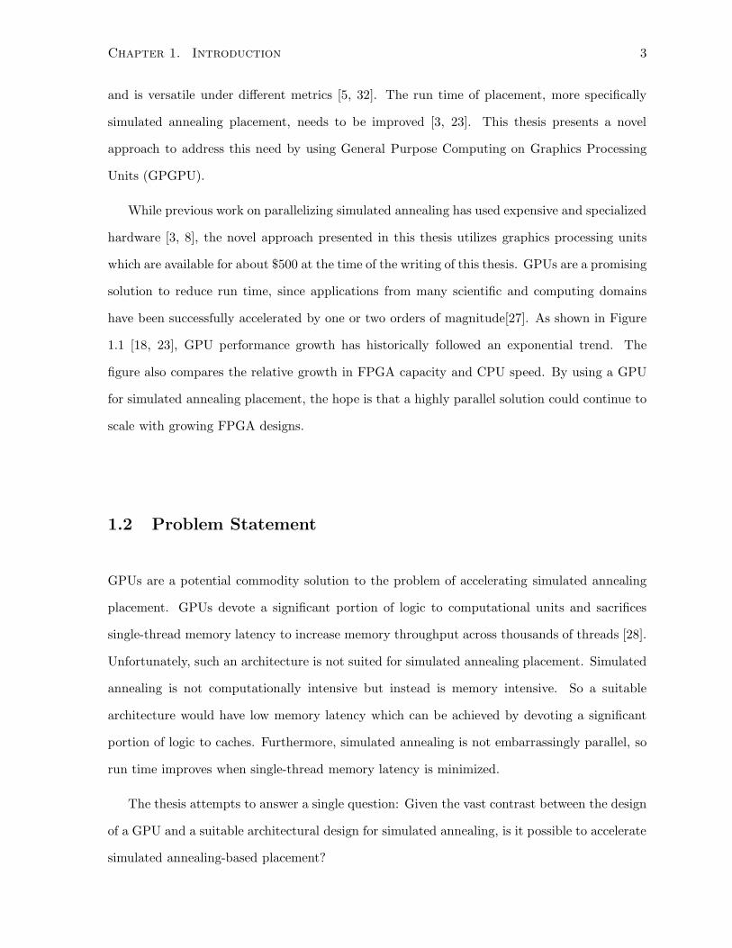
and is versatile under different metrics [5, 32]. The run time of placement, more specifically
simulated annealing placement, needs to be improved [3, 23]. This thesis presents a novel
approach to address this need by using General Purpose Computing on Graphics Processing
Units (GPGPU).
While previous work on parallelizing simulated annealing has used expensive and specialized
hardware [3, 8], the novel approach presented in this thesis utilizes graphics processing units
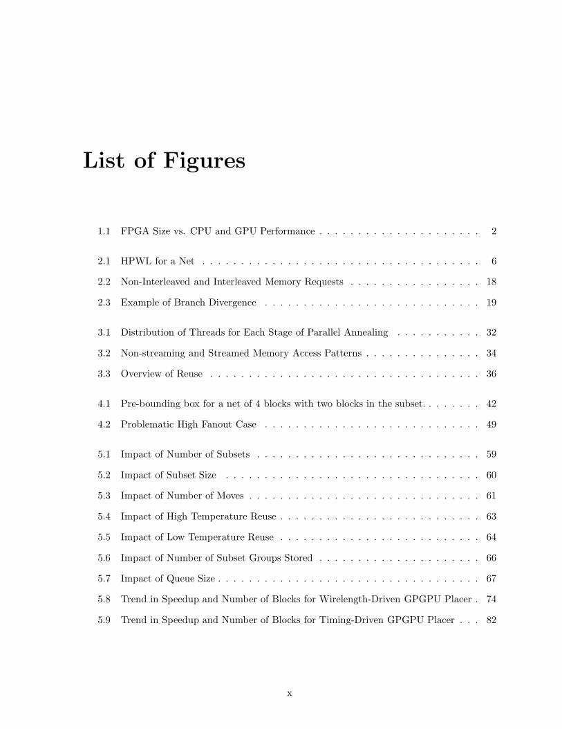
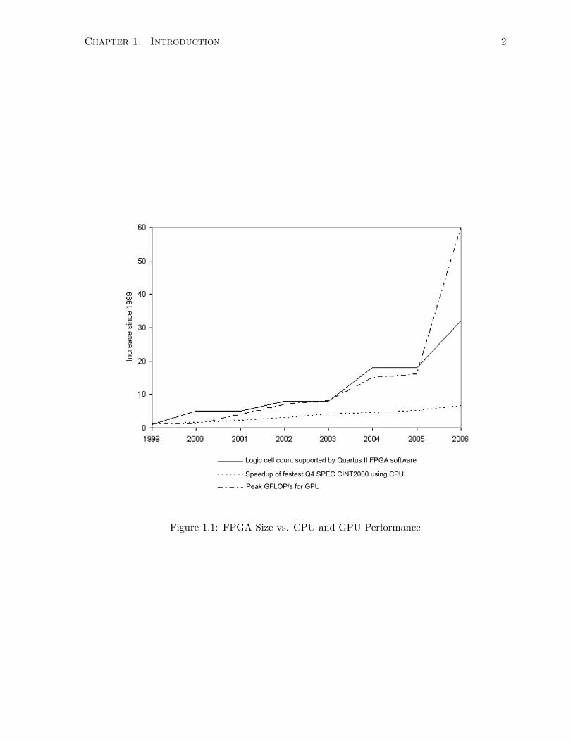
which are available for about $500 at the time of the writing of this thesis. GPUs are a promising
solution to reduce run time, since applications from many scientific and computing domains
have been successfully accelerated by one or two orders of magnitude[27]. As shown in Figure
1.1 [18, 23], GPU performance growth has historically followed an exponential trend. The
figure also compares the relative growth in FPGA capacity and CPU speed. By using a GPU
for simulated annealing placement, the hope is that a highly parallel solution could continue to
scale with growing FPGA designs.
1.2 Problem Statement
GPUs are a potential commodity solution to the problem of accelerating simulated annealing
placement. GPUs devote a significant portion of logic to computational units and sacrifices
single-thread memory latency to increase memory throughput across thousands of threads [28].
Unfortunately, such an architecture is not suited for simulated annealing placement. Simulated
annealing is not computationally intensive but instead is memory intensive. So a suitable
architecture would have low memory latency which can be achieved by devoting a significant
portion of logic to caches. Furthermore, simulated annealing is not embarrassingly parallel, so
run time improves when single-thread memory latency is minimized.
The thesis attempts to answer a single question: Given the vast contrast between the design
of a GPU and a suitable architectural design for simulated annealing, is it possible to accelerate
simulated annealing-based placement?
Chapter 1. Introduction 4
1.3 Contributions
The following contributions are made:
• A novel parallel annealing framework, called the subset-based framework, is proposed
that is designed for the GPU architecture.
• A novel timing metric is proposed that approximates the conventional one used in previous
works yet requires significantly less memory.
• For the first time, it is shown that FPGA placement can be accelerated by one order of
magnitude on commodity hardware, while maintaining competitive quality of results in
both wirelength and timing.
1.4 Thesis Overview
Chapter 2 reviews relevant material in the area of parallel simulated annealing placement. It
continues with a description of features of GPU architecture which are relevant to this thesis.
Chapter 3 describes the subset-based framework as well as optimizations for this framework and
its properties. Chapter 4 discusses how the wirelength and timing metrics can be implemented
within the subset-based framework. Chapter 5 evaluates both the wirelength-driven GPGPU
annealer and timing-driven GPGPU annealer and analyzes its properties. Lastly, Chapter 6
summarizes the results and suggests some future work.
Chapter 2
Background
In this chapter, the sequential version of simulated annealing algorithm placement is reviewed to
prepare the reader for a survey of previous attempts to parallelize simulated annealing. Finally,
features relevant to this thesis of NVIDIA’s Graphics Processing Units (GPUs) are reviewed.
2.1 FPGA Placement Problem
A netlist is a collection of logic blocks and nets which connect those logic blocks. The goal of
placement is to assign all the logic blocks within a netlist to valid location on the placement
area such that a cost metric is optimized. In other words, the goal is to find a mapping P
which assigns all blocks, {bi}, to a set of locations, {(xi, yi)}, where 1 ≤ x ≤ W and 1 ≤ y ≤ H.
The values W and H are the width and height for a rectangular placement area. The set of
locations are unique, and no two blocks can be mapped to the same location. The location of
block bi is denoted by P (bi) = (xi, yi).
The cost metric assigns a value to a given placement which indicates its quality. The symbol
C(P ) is the value of the cost metric for a given placement, P . The goal of placement is to find
P such that C(P ) is minimized.
One set of metrics is called wirelength-driven and these metrics attempt to minimize the
distance between blocks on the same net so that the amount of wiring is minimal. The metric
used in this thesis to model wirelength is the half-perimeter wirelength (HPWL) metric. The
5
Chapter 2. Background 6
Bounding Box
ymax
ymin
xmin xmax
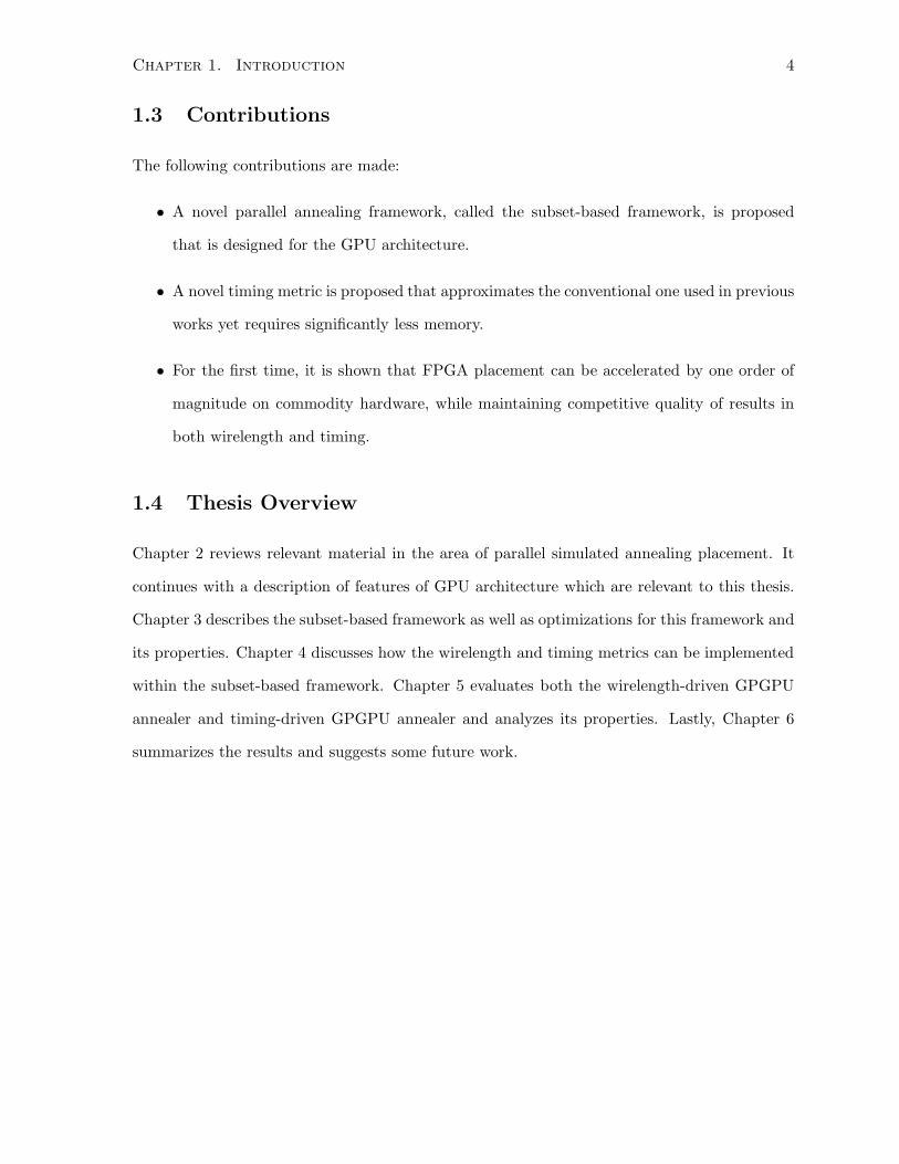
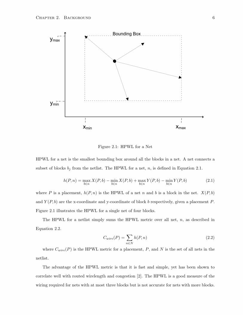
Figure 2.1: HPWL for a Net
HPWL for a net is the smallest bounding box around all the blocks in a net. A net connects a
subset of blocks bj from the netlist. The HPWL for a net, n, is defined in Equation 2.1.
h(P, n) = maxb∈n
X(P, b) − minb∈n
X(P, b) + maxb∈n
Y (P, b) − minb∈n
Y (P, b) (2.1)
where P is a placement, h(P, n) is the HPWL of a net n and b is a block in the net. X(P, b)
and Y (P, b) are the x-coordinate and y-coordinate of block b respectively, given a placement P .
Figure 2.1 illustrates the HPWL for a single net of four blocks.
The HPWL for a netlist simply sums the HPWL metric over all net, n, as described in
Equation 2.2.
Cwire(P ) =∑
n∈N
h(P, n) (2.2)
where Cwire(P ) is the HPWL metric for a placement, P , and N is the set of all nets in the
netlist.
The advantage of the HPWL metric is that it is fast and simple, yet has been shown to
correlate well with routed wirelength and congestion [2]. The HPWL is a good measure of the
wiring required for nets with at most three blocks but is not accurate for nets with more blocks.
Chapter 2. Background 7
More accurate means of estimating wiring at the placement phase are explored in previous
works [2, 5, 33, 39].
Another set of metrics minimize the critical path delay to produce fast circuits. This is
known as timing-driven placement. Previous works in timing-driven placement can roughly be
classified into either path-based or net-based approaches. Path-based approaches minimize the
critical path [14, 15, 35]. The advantage of path-based approaches are that they maintain an
accurate view of the critical path but are unfortunately more computationally expensive. On
the other hand, net-based approaches attempt to reduce the critical path by minimizing nets
which are on the critical path [16, 20, 29, 36].
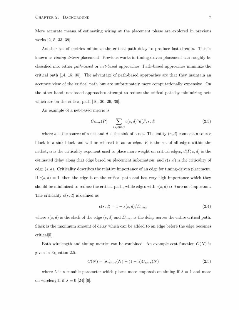
An example of a net-based metric is
Ctime(P ) =∑
(s,d)∈E
c(s, d)αd(P, s, d) (2.3)
where s is the source of a net and d is the sink of a net. The entity (s, d) connects a source
block to a sink block and will be referred to as an edge. E is the set of all edges within the
netlist, α is the criticality exponent used to place more weight on critical edges, d(P, s, d) is the
estimated delay along that edge based on placement information, and c(s, d) is the criticality of
edge (s, d). Criticality describes the relative importance of an edge for timing-driven placement.
If c(s, d) = 1, then the edge is on the critical path and has very high importance which they
should be minimized to reduce the critical path, while edges with c(s, d) ≈ 0 are not important.
The criticality c(s, d) is defined as
c(s, d) = 1 − s(s, d)/Dmax (2.4)
where s(s, d) is the slack of the edge (s, d) and Dmax is the delay across the entire critical path.
Slack is the maximum amount of delay which can be added to an edge before the edge becomes
critical[5].
Both wirelength and timing metrics can be combined. An example cost function C(N) is
given in Equation 2.5.
C(N) = λCtime(N) + (1 − λ)Cwire(N) (2.5)
where λ is a tunable parameter which places more emphasis on timing if λ = 1 and more
on wirelength if λ = 0 [24] [6].
Chapter 2. Background 8
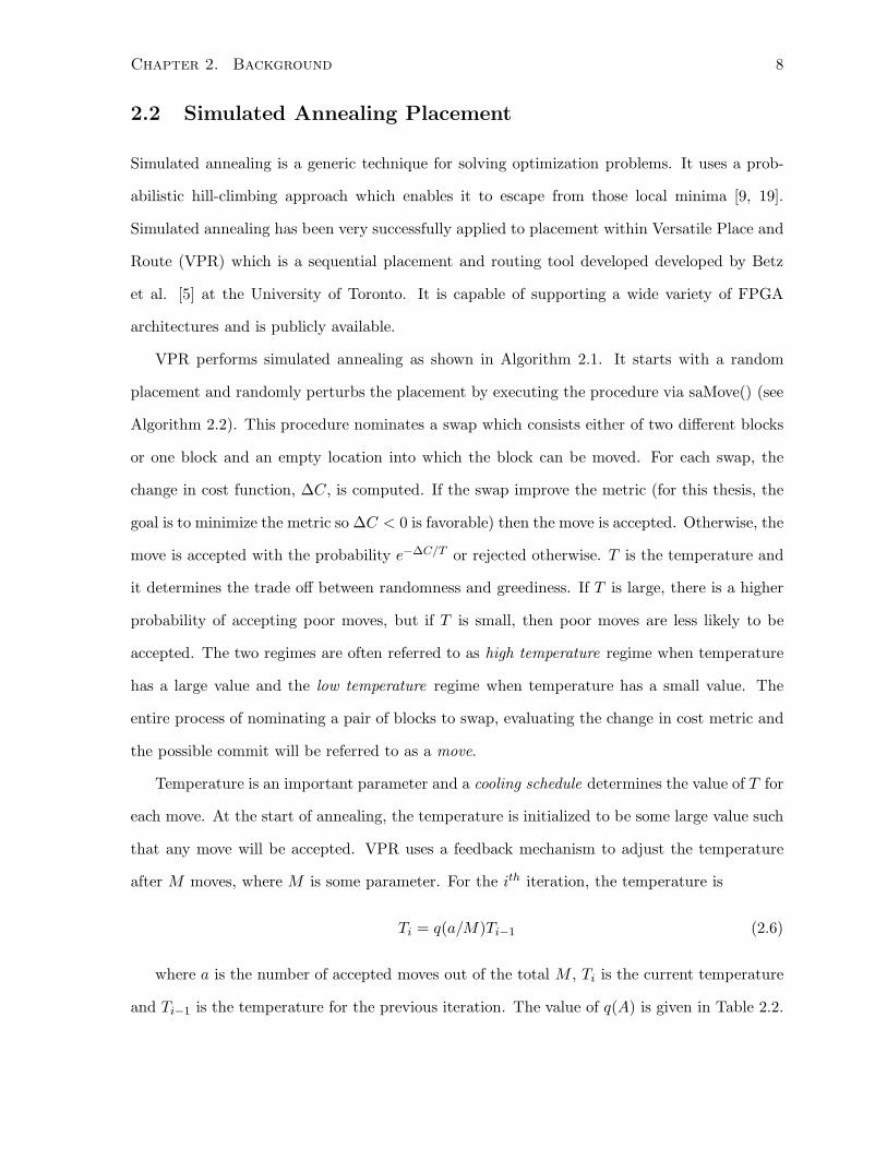
2.2 Simulated Annealing Placement
Simulated annealing is a generic technique for solving optimization problems. It uses a prob-
abilistic hill-climbing approach which enables it to escape from those local minima [9, 19].
Simulated annealing has been very successfully applied to placement within Versatile Place and
Route (VPR) which is a sequential placement and routing tool developed developed by Betz
et al. [5] at the University of Toronto. It is capable of supporting a wide variety of FPGA
architectures and is publicly available.
VPR performs simulated annealing as shown in Algorithm 2.1. It starts with a random
placement and randomly perturbs the placement by executing the procedure via saMove() (see
Algorithm 2.2). This procedure nominates a swap which consists either of two different blocks
or one block and an empty location into which the block can be moved. For each swap, the
change in cost function, ∆C, is computed. If the swap improve the metric (for this thesis, the
goal is to minimize the metric so ∆C < 0 is favorable) then the move is accepted. Otherwise, the
move is accepted with the probability e−∆C/T or rejected otherwise. T is the temperature and
it determines the trade off between randomness and greediness. If T is large, there is a higher
probability of accepting poor moves, but if T is small, then poor moves are less likely to be
accepted. The two regimes are often referred to as high temperature regime when temperature
has a large value and the low temperature regime when temperature has a small value. The
entire process of nominating a pair of blocks to swap, evaluating the change in cost metric and
the possible commit will be referred to as a move.
Temperature is an important parameter and a cooling schedule determines the value of T for
each move. At the start of annealing, the temperature is initialized to be some large value such
that any move will be accepted. VPR uses a feedback mechanism to adjust the temperature
after M moves, where M is some parameter. For the ith iteration, the temperature is
Ti = q(a/M)Ti−1 (2.6)
where a is the number of accepted moves out of the total M , Ti is the current temperature
and Ti−1 is the temperature for the previous iteration. The value of q(A) is given in Table 2.2.
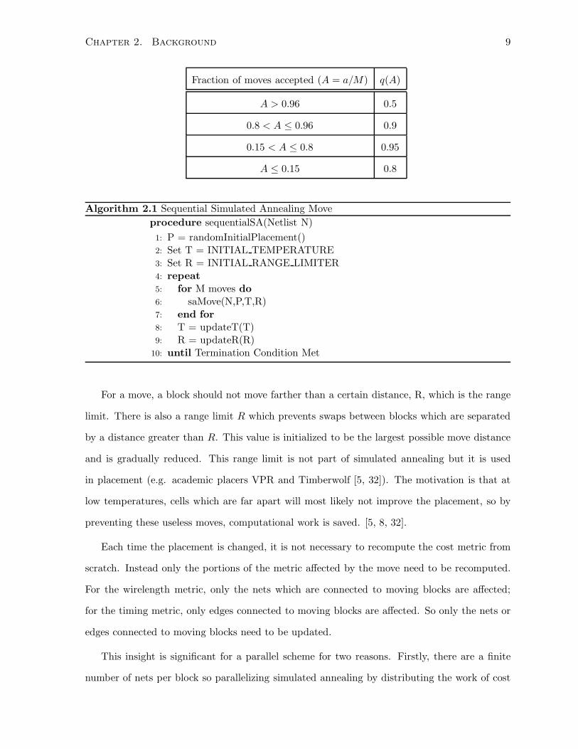
Chapter 2. Background 9
Fraction of moves accepted (A = a/M) q(A)
A > 0.96 0.5
0.8 < A ≤ 0.96 0.9
0.15 < A ≤ 0.8 0.95
A ≤ 0.15 0.8
Algorithm 2.1 Sequential Simulated Annealing Move
procedure sequentialSA(Netlist N)
1: P = randomInitialPlacement()2: Set T = INITIAL TEMPERATURE3: Set R = INITIAL RANGE LIMITER4: repeat5: for M moves do6: saMove(N,P,T,R)7: end for8: T = updateT(T)9: R = updateR(R)
10: until Termination Condition Met
For a move, a block should not move farther than a certain distance, R, which is the range
limit. There is also a range limit R which prevents swaps between blocks which are separated
by a distance greater than R. This value is initialized to be the largest possible move distance
and is gradually reduced. This range limit is not part of simulated annealing but it is used
in placement (e.g. academic placers VPR and Timberwolf [5, 32]). The motivation is that at
low temperatures, cells which are far apart will most likely not improve the placement, so by
preventing these useless moves, computational work is saved. [5, 8, 32].
Each time the placement is changed, it is not necessary to recompute the cost metric from
scratch. Instead only the portions of the metric affected by the move need to be recomputed.
For the wirelength metric, only the nets which are connected to moving blocks are affected;
for the timing metric, only edges connected to moving blocks are affected. So only the nets or
edges connected to moving blocks need to be updated.
This insight is significant for a parallel scheme for two reasons. Firstly, there are a finite
number of nets per block so parallelizing simulated annealing by distributing the work of cost
Chapter 2. Background 10
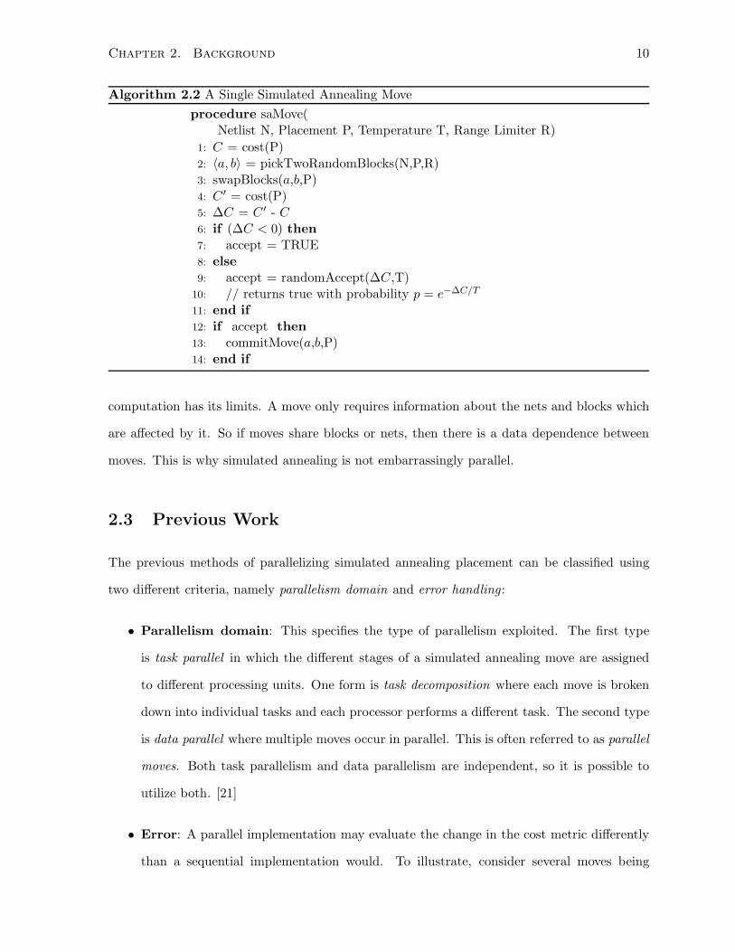
Algorithm 2.2 A Single Simulated Annealing Move
procedure saMove(Netlist N, Placement P, Temperature T, Range Limiter R)
1: C = cost(P)2: 〈a, b〉 = pickTwoRandomBlocks(N,P,R)3: swapBlocks(a,b,P)4: C ′ = cost(P)5: ∆C = C ′ - C6: if (∆C < 0) then7: accept = TRUE8: else9: accept = randomAccept(∆C,T)
10: // returns true with probability p = e−∆C/T
11: end if12: if accept then13: commitMove(a,b,P)14: end if
computation has its limits. A move only requires information about the nets and blocks which
are affected by it. So if moves share blocks or nets, then there is a data dependence between
moves. This is why simulated annealing is not embarrassingly parallel.
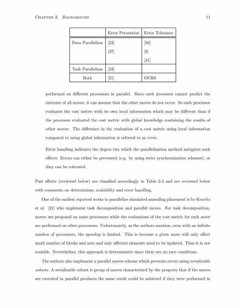
2.3 Previous Work
The previous methods of parallelizing simulated annealing placement can be classified using
two different criteria, namely parallelism domain and error handling :
• Parallelism domain: This specifies the type of parallelism exploited. The first type
is task parallel in which the different stages of a simulated annealing move are assigned
to different processing units. One form is task decomposition where each move is broken
down into individual tasks and each processor performs a different task. The second type
is data parallel where multiple moves occur in parallel. This is often referred to as parallel
moves. Both task parallelism and data parallelism are independent, so it is possible to
utilize both. [21]
• Error: A parallel implementation may evaluate the change in the cost metric differently
than a sequential implementation would. To illustrate, consider several moves being
Chapter 2. Background 11
Error Prevention Error Tolerance
Data Parallelism [23] [34]
[37] [8]
[31]
Task Parallelism [23]
Both [21] OURS
performed on different processors in parallel. Since each processor cannot predict the
outcome of all moves, it can assume that the other moves do not occur. So each processor
evaluates the cost metric with its own local information which may be different than if
the processor evaluated the cost metric with global knowledge containing the results of
other moves. The difference in the evaluation of a cost metric using local information
compared to using global information is referred to as error.
Error handling indicates the degree two which the parallelization method mitigates such
effects. Errors can either be prevented (e.g. by using strict synchronization schemes), or
they can be tolerated.
Past efforts (reviewed below) are classified accordingly in Table 2.3 and are reviewed below
with comments on determinism, scalability and error handling.
One of the earliest reported works to parallelize simulated annealing placement is by Kravitz
et al. [21] who implement task decomposition and parallel moves. For task decomposition,
moves are proposed on some processors while the evaluations of the cost metric for each move
are performed on other processors. Unfortunately, as the authors mention, even with an infinite
number of processors, the speedup is limited. This is because a given move will only affect
small number of blocks and nets and only affected elements need to be updated. Thus it is not
scalable. Nevertheless, this approach is deterministic since there are no race conditions.
The authors also implement a parallel moves scheme which prevents errors using serializable
subsets. A serializable subset is group of moves characterized by the property that if the moves
are executed in parallel produces the same result could be achieved if they were performed in
Chapter 2. Background 12
some serial order. This property implies that a serializable subset is a group of moves which
do not interact or share blocks or nets otherwise there would be data dependencies. Evaluated
moves are either accepted or rejected. For accepted moves within the set, a serializable subset
is found and committed. It is not trivial to compute the largest possible serializable subset
given a set of accepted moves, so the authors resort to committing the first accepted move and
aborts all other moves. Thus the fastest move will commit, and this leads to race conditions. So
this approach is not deterministic. The advantage of this approach is that it should converge
to the optimal value in the same way as a sequential implementation because there are no
errors. The drawback is run time performance. only one move is committed out of a set of
evaluated moves. Thus at high temperatures, where many moves are accepted and should be
committed, the aborted moves lead to wasted computation. So this approach is not scalable at
high temperatures. On the other hand, this approach is more suitable for the low temperature
regime where the acceptance probability for random moves is low.
The authors combine both methods. Task decomposition is used at high temperature when
it is more appropriate when the temperature is high, while parallel moves is more appropriate
when the temperature is low. This work was tested on a single benchmark of 100 blocks so the
robustness of this approach is questionable. A speedup of 2x is achieved using three processors
and for four processors a speed of less than 2.3x is achieved.
The parallel moves approach proposed by Kravitz et al. at high temperature suffers from
poor scalability. Rose et al. address this problem [30, 31]. In the high temperature regime, the
authors observe that performing simulated annealing in this regime is similar to generating a
coarse placements which assigns blocks to a general area. The author replace annealing in the
high temperature regime with Heuristic Spanning which generates different coarse placement
using different processors to each generate a placement, and once all coarse placements have
been generate, it selects the best one. Since a unique coarse placement is generated by each
processor the approach is scalable.
The chosen placement undergoes simulated annealing in the low temperature regime using
parallel moves. This is done by dispatching moves to different processors, and after each
processor has performed N moves, the processors broadcast the information updates to each
Chapter 2. Background 13
other. If N > 10, the authors found that the placement quality was not stable and the cost
metric monotonically increases instead of decreases.
The authors use a set of benchmarks from Bell Northern Research Ltd. and another bench-
mark from the University of Toronto Microelectronics Development Centre which range in size
from 446 to 1795 cells. As discussed, the Heuristic Spanning is scalable. However, for parallel
moves, as the number of processors increases so does the amount of communication between
processors. This communication overhead grows quadratically with the number of processors,
so this approach will not scale linearly with the number of processors. In terms of determinism,
Heuristic Spanning is deterministic, since the generation of each individual coarse placement
is done sequentially, and then the best coarse placement is selected. For the parallel moves, it
seems that the approach could be deterministic if appropriate steps were taken to synchronize
communication. The authors mention that these broadcasts occur after a each processor com-
pletes N moves and this controlled and periodic broadcast could act as synchronization. The
parallelization scheme uses parallel moves while permitted errors. A speedup of 4.3x is achieved
with 5 processors for the overall scheme.
Sun et al.[34] implement an approach which uses message passing to communicate between
machines on a network cluster. The goal of this approach is to minimize communication over-
head and synchronization so that a near linear speedup could be achieved. Each machine is
assigned a unique region of the placement area and performs annealing moves within that re-
gion. There are two types of region assignments: one dividing the placement area into vertical
strips and another dividing the placement area into horizontal strips. By alternating between
these two assignments, blocks could migrate along vertical then horizontal strips so a block is
not restricted to a region.
This approach will not scale linearly. Several times during the course of placement, each
machine broadcasts an update of any blocks which it has moved. Consequently, the overhead
of communication grows quadratically with the number of processors. As communication over-
head increases, processor utilization decreases: with two, four and six processors the processor
utilization per machine is 98%, 93% and 87% respectively. It is doubtful that such an approach
would scale to hundreds of cores. Because block positions are broadcasted periodically, compu-
Chapter 2. Background 14
tations use stale data and so this approach is error tolerant. Also this approach appears to be
deterministic since moves are performed sequentially on each processor and communication is
controlled with synchronization barriers. This approach is evaluated on the MCNC benchmark
suite. Speedups of 1.96x, 3.78x and 5.30x are reported for two, four and six cores.
Sangio et al. implement a parallel moves approach on a multiprocessor [8]. Blocks are
assigned to different processors and each processor performs annealing moves within the assigned
blocks. Blocks may be reassigned to different processors and these reassignments occur when a
block is closer to the centroid of the another processor than its own. The centroid of a processor
is the average position of all the blocks assigned to it. The approach permits errors and the
authors empirically study this error. They find that at low temperatures error approaches
zero on average. Five benchmarks (ranging in size from 4 to 122 blocks) were used to test
the approach. This approach uses locks to synchronize access to a shared list and the authors
admit that management of the list is difficult to do in parallel, so this list is a serial bottleneck.
Consequently, this approach will probably not be scalable for manycore architectures. Speedups
of 1.72x, 3.31x and 6.40x are achieved using two, four and eight cores, with less than one percent
difference in quality between the sequential and parallel versions on average. The results should
be read cautiously as these were obtained from only one benchmark.
A speculative implementation of simulated annealing is reported by Witte et al. [37]. This
speculative implementation anneals N consecutive moves in parallel such that the result is
equivalent to a sequential implementation. Except for the first move, all moves require infor-
mation about the previous moves. Consequently, processors are assigned moves and they will
speculate about the outcome of the previous moves. The first move is performed normally. The
second move is evaluated by two processors where one speculates that the first was rejected
while the second speculates that it was accepted. The third move is evaluated by two pairs
(i.e. four) processors, where each pair speculates on either the rejected or accepted second pair.
Hence, this approach requires 2N+1 − 1 processors, since 2n processors are used to evaluate the
nth move. Once all the speculative computations are completed, the correct outcomes are known
and the processors which made the correct assumptions commit their moves. This approach
should give a theoretical speedup of log2 P , where P is the number of processors. However,
Chapter 2. Background 15
the authors observe that because the acceptance probability varies at different temperatures,
it is possible to assign more (or fewer) processors to speculate along scenarios with higher (or
lower) acceptance rates. With this optimization the average theoretical speedup is reported to
be P/ log2 P , which unfortunately does not scale linearly with the number of processors. In
fact, speedups of 2.4x, 3.25x and 3.3x are achieved on on 4, 8 and 16 processors. Since this
approach produces the exact same results as a sequential implementation, there are no errors.
Ludwin et al. [23] use commodity multicore processors to accelerate simulated annealing
placement for Quartus II which is a commercial tool from Altera R© used for FPGA design.
This work sets itself apart from previous work because it is a commercial application involving
millions of lines of code. They implement two different approaches: one with task decomposition
and the other with parallel moves. For task decomposition, moves are divided into two tasks
where the first accounts for about 40% of the run time and the second accounts for about 60%.
The implementation of task decomposition had limited scalability, and achieved a speedup of
1.3x on two cores. The authors’ implementation of parallel moves uses several cores to evaluate
moves and a single core to check for dependencies and commit moves. In this approach, error is
prevented by only committing moves that do not have share data. While this approach seems
scalable, the authors report that memory is a bottleneck. A speedup of 2.2x was achieved using
parallel moves. Both approaches were implemented such that they would be equivalent to a
serial implementation and so they are deterministic and prevents errors.
2.4 GPU Parallel Architecture
This section provides and overview of Graphics Processing Units (GPU) and highlights the
architectural features which have impacted the design and implementation of the parallel simu-
lated annealing using General Purpose computing on GPU (GPGPU). This section focuses on
the execution model for Compute Unified Device Architecture (CUDA) and the architecture of
GPUs released by NVIDIA.
Chapter 2. Background 16
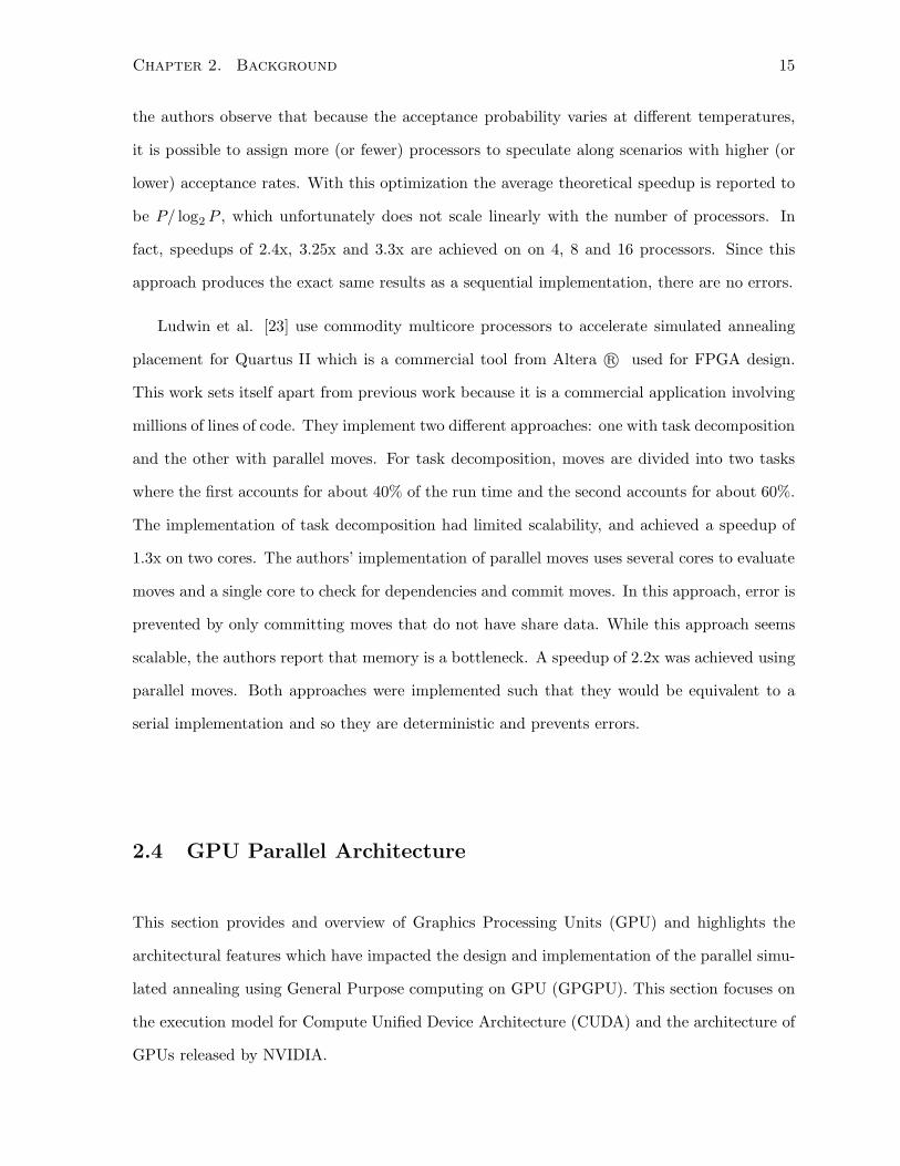
Hardware Resource Item Executed on Hardware Resource
Streaming Processor (SP) Thread
Streaming Multiprocessor (SMP) CUDA Block, Warp
GPU Grid
Table 2.1: Mapping between threads, CUDA blocks and grids to hardware resources
2.4.1 Execution Model
CUDA extends the C language by introducing kernels which are sub-programs that execute on
the GPU. Each kernel is executed on many CUDA threads in parallel. Threads are organized
into a hierarchy. At the first level, thread are grouped into warps. All threads in a warp execute
in a Single Instruction Multiple Data (SIMD) fashion. Warps are group into CUDA blocks. The
size of a CUDA block is determined by the programmer and all blocks have the same number
of threads. At the top of the hierarchy, the entire collection of all CUDA blocks is known as
a grid, and again the programmer decides the number of CUDA blocks per grid. While the
literature uses the term blocks to refer to CUDA blocks, to avoid confusion with netlist blocks,
the term CUDA blocks is adopted for this thesis.
The thread hierarchy parallels the GPU processor hierarchy. At the lowest level are stream-
ing processors (SPs) which execute individual threads. These SPs are grouped into arrays of
streaming multiprocessors (SMPs) which execute CUDA blocks. Finally, the SMPs together
constitute the GPU which executes a grid. Warps are significant because all threads within a
warp execute the same instruction. For the GTX280, N = 32. The parallel between a warp
and the GPU architecture is that all SP within the same SMP must execute the same instruc-
tion each cycles, which is why threads within a warp execute in a SIMD manner. Table 2.1
summarizes the mapping. Table 2.1 summarizes the mapping.
While the programmer can specify the number of CUDA blocks per grid and threads per
CUDA block, the hardware only has a fixed number of SMPs per GPU and SPs per SMP. If
there are more CUDA blocks than SMPs, then the extra CUDA blocks are scheduled serially.
The number of threads, however, are limited by available hardware resources. The maximum
number of threads is 512 per block for the GTX280. In addition, threads within a CUDA block
Chapter 2. Background 17
share the register file. Threads within a CUDA block also collectively use shared memory which
is 16kB in size and all threads can access any of the shared memory which is allocated to the
CUDA block. All the CUDA blocks within the same kernel use the same amount of shared
memory.
A CUDA block is executed on an SMP, and if there are enough hardware resources another
CUDA block can be executed concurrently. Increasing the amount of concurrent CUDA blocks
actually improves run time as will be seen in Subsection 2.4.2. It should be clarified that
when CUDA blocks are executed concurrently on an SMP they time-share the computational
resource.
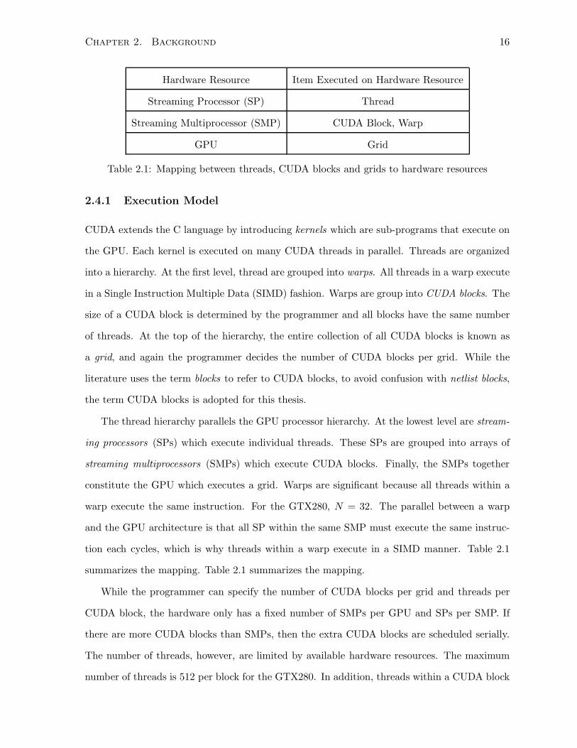
2.4.2 Hiding Memory Latency
Accesses to global memory take hundreds of cycles. In order to increase the throughput of
memory accesses, the GPU architecture allows for interleaving memory requests. While one
warp is stalled on a memory request, another warp can also issue another memory request.
As an illustration, consider a simple program which reads data and performs a computation
three times. In Figure 2.2(a), the non-interleaving version issues the memory request then
immediately performs the computation which is followed by another two iterations. On the
other hand, a more efficient implementation would be to load the data into shared memory
make three concurrent requests, then performing the computation as in Figure 2.2(b). Except
for the first computation, the memory latency for the second and third computation seems to
have decreased. If enough results are issued in parallel, the latency can appear to be zero, so
this is called latency hiding, it also refers to cases where there are not enough requests.
The effect of latency hiding increases as the number of warps increases, since the presence
of more warps permit more concurrency. The best results are achieved if there are at least 192
threads executing on an SMP [28]. These threads do no need to belong to the same block, but
can belong to other blocks executed on the same SMP. Consequently, increasing the number
of blocks which can concurrently be executed on an SMP has the effect of increasing latency
hiding and thus reducing the overhead of memory accesses. Therefore, it is very important to
maximize the number of threads executing on an SMP, which is accomplished by having many
Chapter 2. Background 18
Memory Fetch
Computation
a) Not Interleaving Memory Requests
b) Interleaving Memory Requests
Figure 2.2: Non-Interleaved and Interleaved Memory Requests
threads per CUDA block or having many CUDA blocks execute concurrently on an SMP.
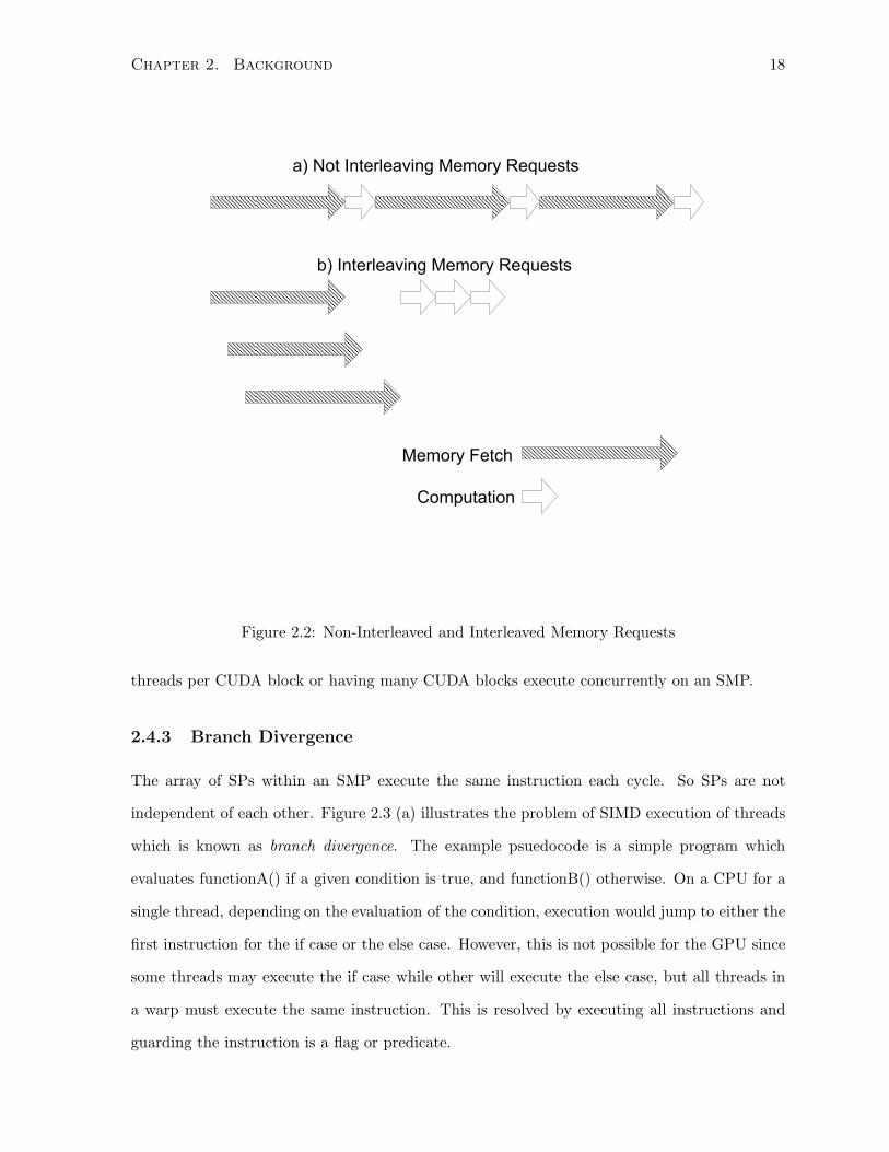
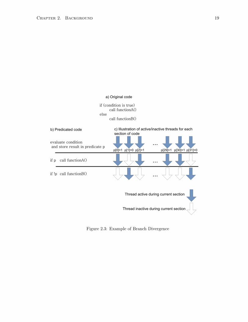
2.4.3 Branch Divergence
The array of SPs within an SMP execute the same instruction each cycle. So SPs are not
independent of each other. Figure 2.3 (a) illustrates the problem of SIMD execution of threads
which is known as branch divergence. The example psuedocode is a simple program which
evaluates functionA() if a given condition is true, and functionB() otherwise. On a CPU for a
single thread, depending on the evaluation of the condition, execution would jump to either the
first instruction for the if case or the else case. However, this is not possible for the GPU since
some threads may execute the if case while other will execute the else case, but all threads in
a warp must execute the same instruction. This is resolved by executing all instructions and
guarding the instruction is a flag or predicate.
Chapter 2. Background 19
if (condition is true)
call functionA()
else
call functionB()
evaluate condition
and store result in predicate p
if p call functionA()
if !p call functionB()
...
Thread active during current section
...
...
p[0]=1
Thread inactive during current section
a) Original code
b) Predicated code c) Illustration of active/inactive threads for each
section of code
p[1]=0 p[2]=1 p[29]=1 p[30]=1 p[31]=0
Figure 2.3: Example of Branch Divergence
Chapter 2. Background 20
Figure 2.3 (b) gives the predicated form of the code and now the calls to functionA() and
functionB() are guarded with a predicate p[i] where i is the thread identifier. In the example,
there are 32 threads and some will evaluate the condition to be true (which is indicated by
showing p[i] = 1) or false otherwise (p[i] = 0). In part (c) of the illustration, active and inactive
threads are shown. For the computation of the condition, all threads are active and attempt
to evaluate the condition and set p[i]. In the next section, only threads with p[i] = 1 will be
active, and will make the call to functionA(), while the other threads are idle and vice versa for
functionB(). So instead of executing functionA() and functionB() in parallel, they are executed
serially which defeats the purpose of having parallel processors.
Therefore, it is important that the GPGPU application be designed to avoid branch di-
vergence whenever possible. The ideal case is to have all threads active. When this is not
possible, the amount of time in which threads are idle and the number of idle threads should
be minimized.
2.5 Summary
This chapter reviews the related material on parallelizing placement. First the placement
problem is introduced which is followed by a description of VPR’s implementation of simulated
annealing placement. Next, previous works on parallelizing simulated annealing placement are
reviewed. Lastly, in order to provide background on the GPU, relevant aspects and features
are discussed.
Chapter 3
Subset-based Simulated Annealing
Placement Framework
In this chapter, the parallel annealing framework using GPGPU is presented. To rationalize
design decisions, the chapter begins with a description of challenges of performing parallel
annealing on GPUs.
3.1 Challenges for Simulated Annealing Placement using GPGPU
It is illustrative to discuss a simple and natural approach to implement simulated annealing
using GPGPU, which will be referred to as the naıve approach. In this approach, moves are
assigned to each streaming processor (SP). If the naıve approach is implemented on a GTX280
which has 240 processors which operate at half the clock frequency of a typical CPU, then the
ideal speedup is 120x over a sequential implementation on a CPU. Unfortunately, this approach
suffers from several problems. The first set of problems relate to run time which stems from
memory latency and branch divergence. In addition to these problems, this naıve approach
raises several concerns about consistency, convergence and scalability.
21
Chapter 3. Subset-based Simulated Annealing Placement Framework 22
3.1.1 Memory Latency
The problem with global memory is that it is slow. On the other hand, shared memory is fast,
but since it is a million times smaller, it is not large enough to store a realistic benchmark.
Illustration of Shared Memory Requirements The purpose of this illustration
is to give an optimistic limit on the size of a netlist which can be stored in
shared memory. The parallel simulated annealing approach for wirelength metric
required 12 bytes per block and 22 bytes per net with an additional 384 bytes for
bookkeeping. Typically there are more nets than blocks for the benchmarks used,
but it will optimistically be assumed that both quantities are equal. Hence, each
block requires 34 bytes. For the GTX280 with 16kB, the largest netlist which
can entirely fit in shared memory is 470 blocks.
Attempting to store the entire netlist in shared memory places a severe limit on the netlist
size. Furthermore, the purpose of this research is to accelerate placement for large netlists since
they require a lot of time. Consequently, there is little value in exploring a placement approach
which cannot handle large benchmarks.
Since storing data in shared memory is not a viable option, the netlist information must be
stored in global memory. However, accesses to global memory are high latency. A single read
access takes about four hundred cycles on the GTX280 [38]. Since simulated annealing is very
memory intensive, the frequent accesses to global memory will consume a large portion of run
time.
3.1.2 Branch Divergence
Another problem is branch divergence, which is discussed in more detail in Subsection 2.4.3.
Branch divergence is a problem for simulated annealing of netlists, because netlists are typically
not very regular. In other words, some nets in the netlist are connected many blocks, while
others are only connected to a few.
Illustration with naıve approach
Chapter 3. Subset-based Simulated Annealing Placement Framework 23
The naıve approach of performing one move on each SP will yield low run time
performance because of two reasons. One reason is that some moves will commit
while others will reject moves which leads to branch divergence. The second more
significant reason is that netlists are not regular. Thus some move evaluations
will be fast while other will be slow, but since the architecture is SIMD, fast
moves will still have to wait for the slow moves to complete.
3.1.3 Consistency, Convergence and Scalability
Aside from the GPU architectural concerns, there are also other concerns: consistency, conver-
gence, and scalability. For the naıve approach, consistency problems may arise if two moves
attempt to move a block in two different directions of if two moves try to move two different
blocks into the same position. The convergence concern questions whether a parallel form of
simulated annealing can produce the same quality of results as a sequential version. One prob-
lem with parallelization schemes are that they may introduce error. Schemes which introduce
error [8, 21, 34] may not have the same quality of results as a sequential version. The problems
of consistency and convergence can be addressed using serializable subsets [21], but as discussed
in Section 2.3 the drawback with this approach is limited scalability. The scalability concern is
that doubling the number of processors may not double the speedup.
3.2 Resolving Challenges
The objective of the subset-based simulated annealing framework is to address the problems and
concerns raised in the previous section. This framework will be referred to as the subset-based
framework for brevity.
One of the problems is that global memory is high latency but shared memory is too small
to store an entire netlist. The solution is to store only portions of a netlist in shared memory.
This portion gives rise to the notion of a subset which is a collection of blocks, all incident nets
and all connectivity information from a netlist.
The other problem is branch divergence. Instead of using the parallel resources in an SMP
Chapter 3. Subset-based Simulated Annealing Placement Framework 24
to perform parallel moves which causes branch divergence, moves are performed serially within
an SMP. The parallel resources are instead used for tasks such as parallel evaluation of cost
metrics and parallel fetch and should lead to significant less branch divergence.
The concern for consistency arises since parallel moves may incorrectly swap a single block
into two different locations or move two blocks into a single location. To resolve this, each
subset is assigned a set of blocks and the locations belonging to those blocks. Further no two
subsets may share a block or locations. Since no two subsets share a block, different subsets
cannot move the same block into two different locations. Furthermore, subsets do not share
locations. Thus two block cannot be moved into the same location. Therefore the consistency
problem is resolved. 1
This scheme does not directly address convergence concerns. During the course of this
thesis, previous work attempted to prevent error, but the quality of results was worse than
the sequential. One attempt prevented error by not allowing subsets to share nets. Blocks
connected to many nets or connected to nets with many blocks did not have a chance to join
any subset and so were not moved. The quality of results was worse than sequential version
because some blocks were not moved or moves rarely.
It was found that permitting error gave better results. While error may prevent convergence,
it will be seen that it does not seem to affect the quality of results because errors are temporary.
Errors may arise when moves are made in parallel across different processors. It will be seen
that this approach can still converge to good quality solutions (Subsection 5.4.2).
Intuitively, this approach is scalable over the number of processors. Since as the netlist
increases in size, there are more opportunities to have more subsets. In addition, as the GPU
architecture increases the number of SMPs, more subsets could be annealed in parallel.
3.3 Subset-based Simulated Annealing Framework
Simulated annealing placement can be modified to become Algorithm 3.1. Subset simulated
annealing is almost exactly like traditional simulated annealing. The call to saMove() (see Algo-
1To handle empty locations, fake blocks are created and placed on empty locations. So blocks can swaps withthese fake blocks to move into empty locations.
Chapter 3. Subset-based Simulated Annealing Placement Framework 25
Algorithm 3.1 Subset Simulated Annealing Framework
procedure subsetSA(Netlist N,Number of subsets Ns,Subset size Ss)
1: P = randomInitialPlacement()2: Set T = INITIAL TEMPERATURE3: Set R = INITIAL RANGE LIMIT4: repeat5: for M times do6: {s} = generateSubsets(N,R,Ns,Ss)7: annealSubsets({s},N,P,T,R)8: end for9: T = updateT(T)
10: R = updateR(R)11: until Termination Condition Met
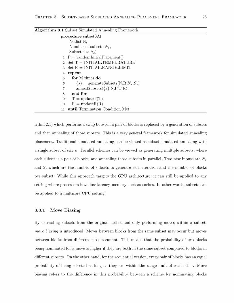
rithm 2.1) which performs a swap between a pair of blocks is replaced by a generation of subsets
and then annealing of those subsets. This is a very general framework for simulated annealing
placement. Traditional simulated annealing can be viewed as subset simulated annealing with
a single subset of size n. Parallel schemes can be viewed as generating multiple subsets, where
each subset is a pair of blocks, and annealing those subsets in parallel. Two new inputs are Ns
and Ss which are the number of subsets to generate each iteration and the number of blocks
per subset. While this approach targets the GPU architecture, it can still be applied to any
setting where processors have low-latency memory such as caches. In other words, subsets can
be applied to a multicore CPU setting.
3.3.1 Move Biasing
By extracting subsets from the original netlist and only performing moves within a subset,
move biasing is introduced. Moves between blocks from the same subset may occur but moves
between blocks from different subsets cannot. This means that the probability of two blocks
being nominated for a move is higher if they are both in the same subset compared to blocks in
different subsets. On the other hand, for the sequential version, every pair of blocks has an equal
probability of being selected as long as they are within the range limit of each other. Move
biasing refers to the difference in this probability between a scheme for nominating blocks
Chapter 3. Subset-based Simulated Annealing Placement Framework 26
for swaps (such as the subset framework) and a sequential version. A move is biased if its
probability for occurring is higher than the sequential version.
Move biasing raises some concerns. When some moves are biased, other moves will occur
with lower probability and this may lower the likelihood that simulated annealing will explore
placements which are potentially better. On the other hand, move biasing comes with some
benefits. If moves are biased, then the probability of reuse of data is higher. This can lead to
better run time. Fundamentally, move biasing can trade off between performance and quality
of results. The hope is that quality is weakly related to bias so there is an opportunity for
significant speedup.
3.4 Subset Generation
The process of subset generation will be described in more detail. In order to generate subsets,
the subsets generation process should possess the following properties. Firstly, selection should
be random and secondly subsets should contains blocks which are within the range limit of each
other. Randomness helps to reduce the likelihood that certain moves are prevented.
For instance, Sun and Sechen [34] propose a scheme where the placement area is
divided into vertical strips and then horizontal strips. When the placement is
divided into vertical strips, blocks cannot move very far horizontally and vice
versa for horizontal strips. This decreases the mobility of blocks and the concerns
is that this could degrade quality of results.
Another concern with this approach is scalability. As the number of processors
increases, so do the number of vertical or horizontal regions. If the placement
area is fixed, this means that the regions will becoming increasingly narrower
as the number of processors increases. When the regions are smaller than the
range limit, this impact the mobility of a block and raises concerns about whether
quality can be maintained [34]. If instead subsets are selected at random from
the placement area, the benefit is that these mobility is not a concern. Since
different subsets are used time, a block has a chance of moving to any location
Chapter 3. Subset-based Simulated Annealing Placement Framework 27
Algorithm 3.2 Subset Generation
procedure generateSubsets(Netlist N,Range limit R,Number of subsets Ns,Size of subset Ss)
1: Define {qi} // queues for each subset2: Define {si} // a group of subsets3: for i = 1 TO Ns do4: qi = ⊘5: n = randomNode(N) // randomly remove a node from N6: enqueue(n,qi)7: end for8: for j = 1 TO Ss do9: for i = 1 TO Ns do
10: n = dequeue(qi)11: push(n,si)12: for k = 1 TO K do13: m = randomWithinRange(R,n)14: // randomly extracted node from N15: // within the window of n16: enqueue(m,qi)17: end for18: end for19: end for20: return {si}
on the placement area.
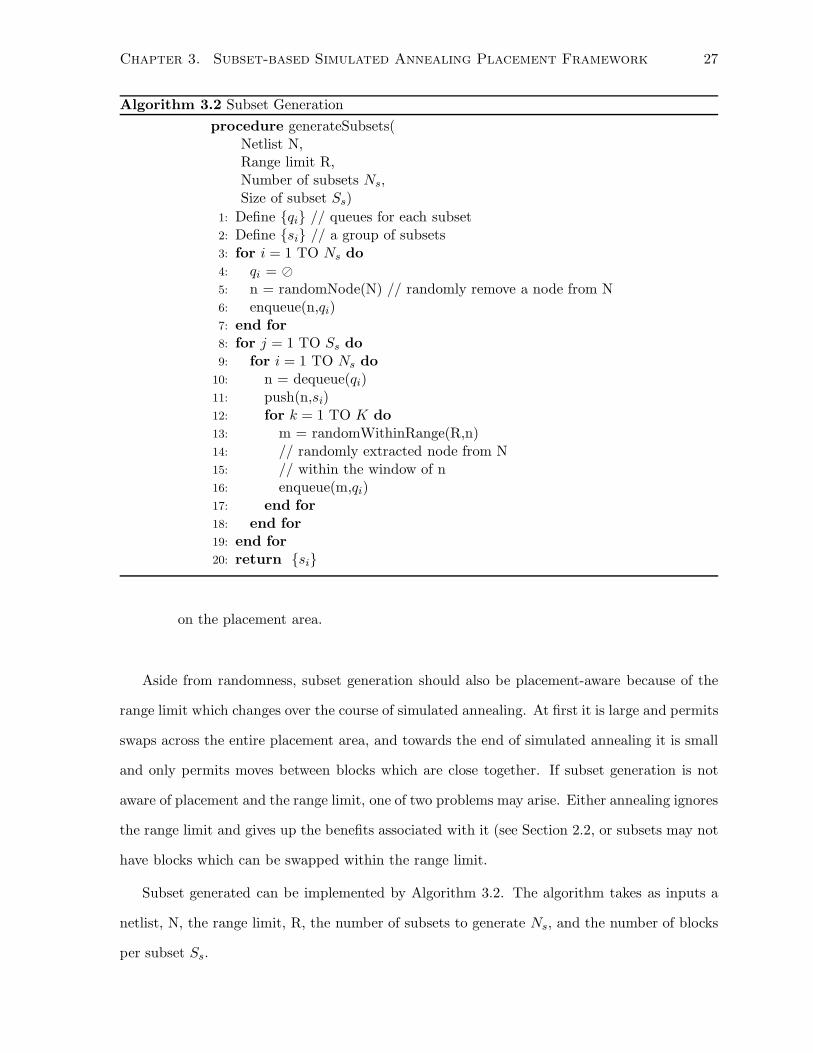
Aside from randomness, subset generation should also be placement-aware because of the
range limit which changes over the course of simulated annealing. At first it is large and permits
swaps across the entire placement area, and towards the end of simulated annealing it is small
and only permits moves between blocks which are close together. If subset generation is not
aware of placement and the range limit, one of two problems may arise. Either annealing ignores
the range limit and gives up the benefits associated with it (see Section 2.2, or subsets may not
have blocks which can be swapped within the range limit.
Subset generated can be implemented by Algorithm 3.2. The algorithm takes as inputs a
netlist, N, the range limit, R, the number of subsets to generate Ns, and the number of blocks
per subset Ss.

Chapter 3. Subset-based Simulated Annealing Placement Framework 28
Subset generation is random and placement aware. This is accomplished in the following
manner. All subsets are randomly assigned a unique starting block. Each subset takes turns
in selecting blocks which are within the range limit, R, of blocks which already belong to the
subset. So blocks in a subset are related by location but not necessarily connectivity. During
the selection process, subsets must ensure that they do no select the same block twice. Each
subset will make Ss attempts to select new blocks, where Ss is the maximum subset size. So
subset generation only provides best effort to ensure that subsets are of size Ss since generating
subsets can be the bottleneck for the overall framework and guaranteeing that each subset is
exactly size Ss incurs additional run time overhead.
The implementation uses a queue to record potential blocks which may be selected next.
These queues are initialized with a random starting block from the netlist. Next each subset
removes the head of its queue, then checks if that block has already been already selected by
another subset. If that blocks has not been selected, then it is added to the current subset and
K other random blocks are selected and placed in the queue. For the implementation K = 4.
The K blocks are selected such that they are within the range limit of the newest addition to
the subset.
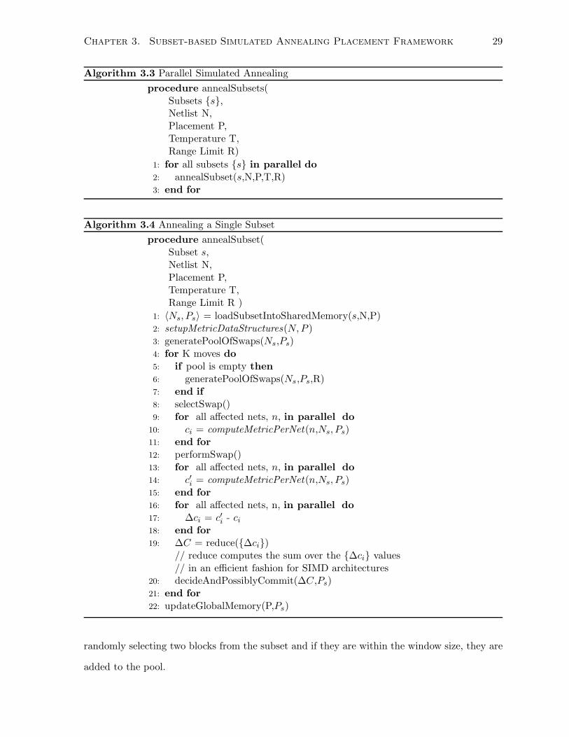
3.5 Parallel Moves on GPGPU
Parallel annealing performs the annealing work. The parallel aspect lies in dispatching subsets
to different processors (see Algorithm 3.5 which dispatches many parallel calls to annealSub-
set()). The procedure annealSubset() anneals a subset. Its inputs are the subset s, the netlist,
placement information P , the temperature and the range limit.
The initialization phase consists of several steps. Given the high memory access latency to
the off-chip global memory, the approach starts with loading the data for one subset into the
low latency on-chip shared memory, which is a common practice in the GPU community. Ns
is the local copy of the netlist and Ps is the local copy of placemen information, where both
are stored in shared memory. Afterwards, a call to setupMetricDataStructures() initializes any
data structures required by the cost metric. Next, a pool of moves is computed. Each thread
Chapter 3. Subset-based Simulated Annealing Placement Framework 29
Algorithm 3.3 Parallel Simulated Annealing
procedure annealSubsets(Subsets {s},Netlist N,Placement P,Temperature T,Range Limit R)
1: for all subsets {s} in parallel do2: annealSubset(s,N,P,T,R)3: end for
Algorithm 3.4 Annealing a Single Subset
procedure annealSubset(Subset s,Netlist N,Placement P,Temperature T,Range Limit R )
1: 〈Ns, Ps〉 = loadSubsetIntoSharedMemory(s,N,P)2: setupMetricDataStructures(N,P )3: generatePoolOfSwaps(Ns,Ps)4: for K moves do5: if pool is empty then6: generatePoolOfSwaps(Ns,Ps,R)7: end if8: selectSwap()9: for all affected nets, n, in parallel do
10: ci = computeMetricPerNet(n,Ns, Ps)11: end for12: performSwap()13: for all affected nets, n, in parallel do14: c′i = computeMetricPerNet(n,Ns, Ps)15: end for16: for all affected nets, n, in parallel do17: ∆ci = c′i - ci
18: end for19: ∆C = reduce({∆ci})
// reduce computes the sum over the {∆ci} values// in an efficient fashion for SIMD architectures
20: decideAndPossiblyCommit(∆C,Ps)21: end for22: updateGlobalMemory(P,Ps)
randomly selecting two blocks from the subset and if they are within the window size, they are
added to the pool.
Chapter 3. Subset-based Simulated Annealing Placement Framework 30
Finally, several moves are performed in sequence and each move is accelerated by exploiting
parallelism within the move. The cost metrics are net-based so when a block moves, it affects
the cost metric for all nets to which it is connected, but not any other nets. The parallelism is
in evaluating the net information on different SP.
For the annealing of a subset, several steps are taken. First, the cost metric for each affected
net is computed and each value is placed in array {c}, where ci is the ith element of the array.
If the pool is empty, then a new set of moves is generated. Swaps are removed from the pool
until a swap is found that has two blocks within the range limit of each other. The two blocks
are then swapped. Now the new cost metric is evaluated for each affected net and placed in
array {c′}. The differences between elements in array {c′} and {c} are computed in parallel
and placed in array {∆c}.
A reduction operator is applied to array {∆c} which sums all the elements in the array. The
result, ∆C, is the net change in the metric. Conceptually, reduction is done as follows. First
it pairs up elements in the set and sums each pair. The results are then paired up again and
summed. The processes is repeated until there is one number which is the final sum. Reduction
is suitable for the GPU since it executes the same instruction on all threads (minimizing branch
divergence) and the advantage is that it requires O(log N) time to sum N elements.
Based on ∆C, a decision is made on whether to commit or reject the move. Lastly, once all
the moves are completed, the updated placement information is committed back to global mem-
ory. This parallel annealing of subsets is general for any cost function. In order to implement
a specific metric, the two functions, setupMetricDataStructures() and computeMetricPerNet()
have to be implemented.
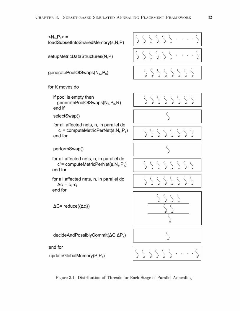
Figure 3.1 illustrates how the threads are utilized throughout the course of parallel annealing.
The area between boxes corresponds to synchronization points while the area within a box
corresponds to a set of instructions which are executed in parallel. In addition, the reduction
has synchronization which is shown as horizontal lines. The number of threads is approximately
indicated by the number of curved arrows.
For initialization stages which access global memory such as loadSubsetIntoSharedMem-
ory() and setupMetricDataStructures(), many threads are used to increase latency hiding (see
Chapter 3. Subset-based Simulated Annealing Placement Framework 31
Subsection 2.4.2). Then whenever moves are generated, many threads are used to fully utilize
available resources. For each move, some tasks are executed using only one thread to avoid
race conditions such as selecting a move. On the other hand, the computation of the cost
metric can be performed by dividing the work across many threads: each thread is responsible
for computing the cost function for a different net. In order to sum the results, a reduction
operator used which utilizes many threads in a SIMD fashion. Once moves are completed, data
is written back to global memory using many threads to again increase latency hiding.
3.6 Improving Run Time
Up to this point, the GPGPU framework addresses several concerns such as high latency mem-
ory, consistency and scalability. Now attention is turned optimizations.
3.6.1 Subset Generation on CPU
While it is possible to implement a subset generation using GPGPU, it suffers greatly due to
performance. One factor is that subset generation is random in nature, and the GPU memory
controller is not optimized for access random accesses to global memory. Furthermore subset
generation requires that a block cannot appear more than one is a subset. Therefore, this
requires synchronization between threads which further degrades performance. On the other
hand, the CPU is more suited for random accesses and a sequential version would not suffer
from the need to synchronize across threads.
3.6.2 Subset Generation Optimizations
Even though the CPU implementation of subset generation was more efficient than a GPU one,
it was still the bottleneck of the solution. The following techniques were devised to address
these problems:
• Pipelining and Streams: The GPGPU scheme for simulated annealing consists of four
steps: i) computation of subsets on the GPU, ii) memory transfer from CPU to GPU, iii)
parallel annealing on the GPU, and iv) memory transfer from GPU to CPU. A natural way
Chapter 3. Subset-based Simulated Annealing Placement Framework 32
<Ns,Ps> =
loadSubsetIntoSharedMemory(s,N,P)
setupMetricDataStructures(N,P)
generatePoolOfSwaps(Ns,,Ps)
if pool is empty then
generatePoolOfSwaps(Ns,Ps,R)
end if
C= reduce({ ci})
selectSwap()
performSwap()
for all affected nets, n, in parallel do
ci = computeMetricPerNet(s,Ns,Ps)
end for
for K moves do
for all affected nets, n, in parallel do
ci = computeMetricPerNet(s,Ns,Ps)
end for
for all affected nets, n, in parallel do
ci = ci -ci
end for
decideAndPossiblyCommit( C, Ps)
end for
updateGlobalMemory(P,Ps)
Figure 3.1: Distribution of Threads for Each Stage of Parallel Annealing
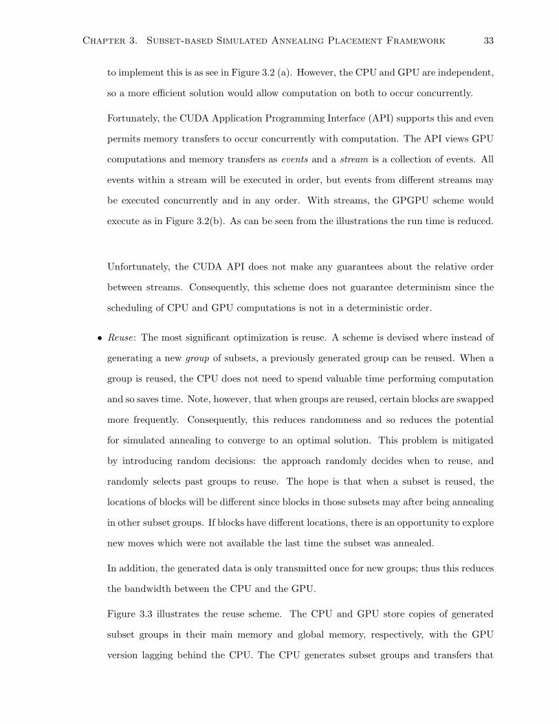
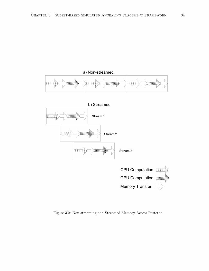
Chapter 3. Subset-based Simulated Annealing Placement Framework 33
to implement this is as see in Figure 3.2 (a). However, the CPU and GPU are independent,
so a more efficient solution would allow computation on both to occur concurrently.
Fortunately, the CUDA Application Programming Interface (API) supports this and even
permits memory transfers to occur concurrently with computation. The API views GPU
computations and memory transfers as events and a stream is a collection of events. All
events within a stream will be executed in order, but events from different streams may
be executed concurrently and in any order. With streams, the GPGPU scheme would
execute as in Figure 3.2(b). As can be seen from the illustrations the run time is reduced.
Unfortunately, the CUDA API does not make any guarantees about the relative order
between streams. Consequently, this scheme does not guarantee determinism since the
scheduling of CPU and GPU computations is not in a deterministic order.
• Reuse: The most significant optimization is reuse. A scheme is devised where instead of
generating a new group of subsets, a previously generated group can be reused. When a
group is reused, the CPU does not need to spend valuable time performing computation
and so saves time. Note, however, that when groups are reused, certain blocks are swapped
more frequently. Consequently, this reduces randomness and so reduces the potential
for simulated annealing to converge to an optimal solution. This problem is mitigated
by introducing random decisions: the approach randomly decides when to reuse, and
randomly selects past groups to reuse. The hope is that when a subset is reused, the
locations of blocks will be different since blocks in those subsets may after being annealing
in other subset groups. If blocks have different locations, there is an opportunity to explore
new moves which were not available the last time the subset was annealed.
In addition, the generated data is only transmitted once for new groups; thus this reduces
the bandwidth between the CPU and the GPU.
Figure 3.3 illustrates the reuse scheme. The CPU and GPU store copies of generated
subset groups in their main memory and global memory, respectively, with the GPU
version lagging behind the CPU. The CPU generates subset groups and transfers that
Chapter 3. Subset-based Simulated Annealing Placement Framework 34
CPU Computation
GPU Computation
Memory Transfer
a) Non-streamed
b) Streamed
Stream 1
Stream 2
Stream 3
Figure 3.2: Non-streaming and Streamed Memory Access Patterns
Chapter 3. Subset-based Simulated Annealing Placement Framework 35
information to the GPU (e.g. groups 5 and 3 are new). Alternatively, the CPU may select
a group and chose to reuse it, as is the case with subset group 8.
One insight is that when past groups are reused, the range limit used to generate the
subset may be larger than the current range limit so there may not be any pair of blocks
which are within the range limit of each other. This is problematic since there would be
no available moves and so no actual work is done.
In practice this is not a strong concern. When blocks are selected for a subset they are
selected to be within the range limit of other blocks. This means that blocks are, on
average, separated by a distance that is less than the range limit. Also, the range limit
gradually decreases so that by the time the subset is reused, there are still blocks which
are within the new range limit of each other.
A more sophisticated scheme could annotate each subset with the range limit used to
generate the subset, and if the subset has a range limit larger than the current one the
subset could be regenerated. The problem is that generating subsets is quite expensive,
so each time the range limit changes, none of the subsets can be reused and the CPU
becomes the bottleneck as it generate new subsets.
An alternative scheme is possible. Given that blocks within a subset are separated by
at most the range limit, it is conceivable that the average distance between blocks for a
subset could be computed and each subset is annotated with the average distance. The
problem is that this involves computing the average distance between each pair of blocks
in the subsets which is O(n2) for n blocks in a subset. On the other hand subset generation
is O(n) and there is already a strong concern about run time. Consequently, this is not
a viable solution.
In summary, a simple approach was used for generating and reusing subsets since it offers
the best run time performance.
• Large Range Limit When the range limit is so large that swaps may occur between any
two blocks (which occurs when temperature is high), it is pointless for subset generation
to check for range limit violations. Consequently, when this is true, the subset genera-
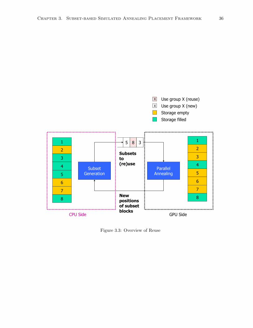
Chapter 3. Subset-based Simulated Annealing Placement Framework 36
SubsetGeneration
ParallelAnnealing
5 8 31
2
3
4
5
6
7
8
1
2
3
4
5
6
7
8
X
X
Use group X (reuse)
Use group X (new)
Storage empty
Storage filled
CPU Side GPU Side
Subsets to (re)use
New positions of subset blocks
Figure 3.3: Overview of Reuse
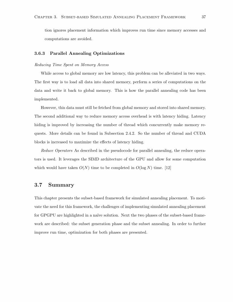
Chapter 3. Subset-based Simulated Annealing Placement Framework 37
tion ignores placement information which improves run time since memory accesses and
computations are avoided.
3.6.3 Parallel Annealing Optimizations
Reducing Time Spent on Memory Access
While access to global memory are low latency, this problem can be alleviated in two ways.
The first way is to load all data into shared memory, perform a series of computations on the
data and write it back to global memory. This is how the parallel annealing code has been
implemented.
However, this data must still be fetched from global memory and stored into shared memory.
The second additional way to reduce memory access overhead is with latency hiding. Latency
hiding is improved by increasing the number of thread which concurrently make memory re-
quests. More details can be found in Subsection 2.4.2. So the number of thread and CUDA
blocks is increased to maximize the effects of latency hiding.
Reduce Operators As described in the pseudocode for parallel annealing, the reduce opera-
tors is used. It leverages the SIMD architecture of the GPU and allow for some computation
which would have taken O(N) time to be completed in O(log N) time. [12]
3.7 Summary
This chapter presents the subset-based framework for simulated annealing placement. To moti-
vate the need for this framework, the challenges of implementing simulated annealing placement
for GPGPU are highlighted in a naıve solution. Next the two phases of the subset-based frame-
work are described: the subset generation phase and the subset annealing. In order to further
improve run time, optimization for both phases are presented.
Chapter 4
Wirelength-Driven and
Timing-Driven Metrics
The subset-based simulated annealing framework presented in the previous chapter is generic
in terms of cost function. This chapter discusses how the framework can be implemented for
wirelength and timing metrics.
4.1 HPWL Metric and Pre-Bounding Box
Given the subset-based framework developed in the previous chapter, implementing a specific
cost metric can be accomplished by defining the functions computeMetricPerNet() and setup-
MetricDataStructures().
The HPWL metric is described in Section 2.1. This metric can be computed by finding
the maximum and minimum x- and y-coordinate for all blocks in the net, then returning
xmax − xmin + ymax − ymin (cf. Equation 2.1). Only the nets affected by the move need to
have the metric computed and to take advantage of the parallel resource, each affected net is
assigned to a different thread. Each thread executes the code described in Algorithm 4.1. As
described in the Section 2.1, the function X takes as input a placement and a block, and returns
the block’s x-coordinate, and similarly for Y .
Unfortunately, this computation requires information about all the blocks on a net but
38
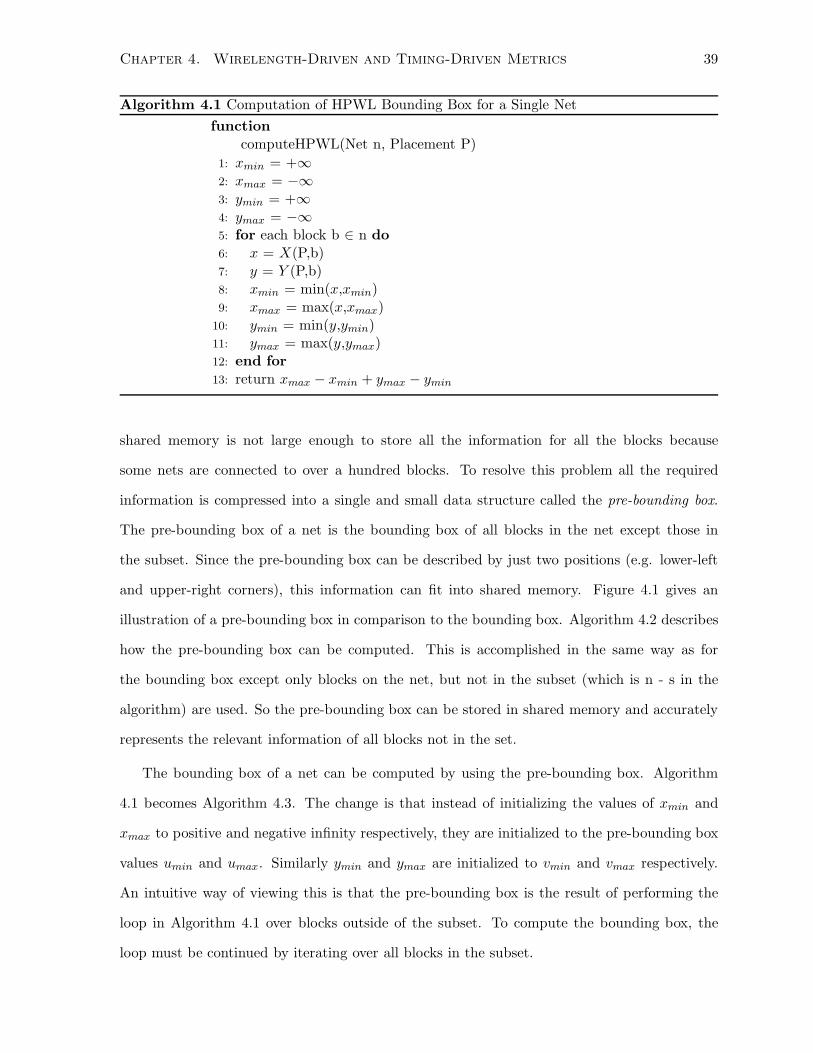
Chapter 4. Wirelength-Driven and Timing-Driven Metrics 39
Algorithm 4.1 Computation of HPWL Bounding Box for a Single Net
functioncomputeHPWL(Net n, Placement P)
1: xmin = +∞2: xmax = −∞3: ymin = +∞4: ymax = −∞5: for each block b ∈ n do6: x = X(P,b)7: y = Y (P,b)8: xmin = min(x,xmin)9: xmax = max(x,xmax)
10: ymin = min(y,ymin)11: ymax = max(y,ymax)12: end for13: return xmax − xmin + ymax − ymin
shared memory is not large enough to store all the information for all the blocks because
some nets are connected to over a hundred blocks. To resolve this problem all the required
information is compressed into a single and small data structure called the pre-bounding box.
The pre-bounding box of a net is the bounding box of all blocks in the net except those in
the subset. Since the pre-bounding box can be described by just two positions (e.g. lower-left
and upper-right corners), this information can fit into shared memory. Figure 4.1 gives an
illustration of a pre-bounding box in comparison to the bounding box. Algorithm 4.2 describes
how the pre-bounding box can be computed. This is accomplished in the same way as for
the bounding box except only blocks on the net, but not in the subset (which is n - s in the
algorithm) are used. So the pre-bounding box can be stored in shared memory and accurately
represents the relevant information of all blocks not in the set.
The bounding box of a net can be computed by using the pre-bounding box. Algorithm
4.1 becomes Algorithm 4.3. The change is that instead of initializing the values of xmin and
xmax to positive and negative infinity respectively, they are initialized to the pre-bounding box
values umin and umax. Similarly ymin and ymax are initialized to vmin and vmax respectively.
An intuitive way of viewing this is that the pre-bounding box is the result of performing the
loop in Algorithm 4.1 over blocks outside of the subset. To compute the bounding box, the
loop must be continued by iterating over all blocks in the subset.
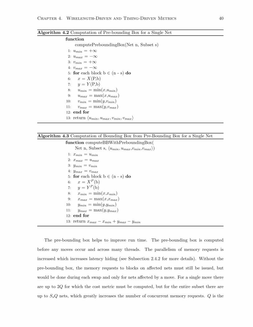
Chapter 4. Wirelength-Driven and Timing-Driven Metrics 40
Algorithm 4.2 Computation of Pre-bounding Box for a Single Net
functioncomputePreboundingBox(Net n, Subset s)
1: umin = +∞2: umax = −∞3: vmin = +∞4: vmax = −∞5: for each block b ∈ (n - s) do6: x = X(P,b)7: y = Y (P,b)8: umin = min(x,umin)9: umax = max(x,umax)
10: vmin = min(y,vmin)11: vmax = max(y,vmax)12: end for13: return 〈umin, umax, vmin, vmax〉
Algorithm 4.3 Computation of Bounding Box from Pre-Bounding Box for a Single Net
function computeBBWithPreboundingBox(Net n, Subset s, 〈umin, umax,vmin,vmax〉)
1: xmin = umin
2: xmax = umax
3: ymin = vmin
4: ymax = vmax
5: for each block b ∈ (n - s) do6: x = XP (b)7: y = Y P (b)8: xmin = min(x,xmin)9: xmax = max(x,xmax)
10: ymin = min(y,ymin)11: ymax = max(y,ymax)12: end for13: return xmax − xmin + ymax − ymin
The pre-bounding box helps to improve run time. The pre-bounding box is computed
before any moves occur and across many threads. The parallelism of memory requests is
increased which increases latency hiding (see Subsection 2.4.2 for more details). Without the
pre-bounding box, the memory requests to blocks on affected nets must still be issued, but
would be done during each swap and only for nets affected by a move. For a single move there
are up to 2Q for which the cost metric must be computed, but for the entire subset there are
up to SsQ nets, which greatly increases the number of concurrent memory requests. Q is the
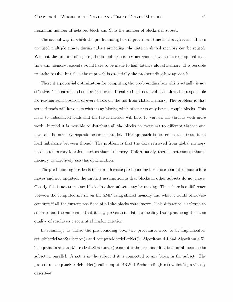
Chapter 4. Wirelength-Driven and Timing-Driven Metrics 41
maximum number of nets per block and Ss is the number of blocks per subset.
The second way in which the pre-bounding box improves run time is through reuse. If nets
are used multiple times, during subset annealing, the data in shared memory can be reused.
Without the pre-bounding box, the bounding box per net would have to be recomputed each
time and memory requests would have to be made to high latency global memory. It is possible
to cache results, but then the approach is essentially the pre-bounding box approach.
There is a potential optimization for computing the pre-bounding box which actually is not
effective. The current scheme assigns each thread a single net, and each thread is responsible
for reading each position of every block on the net from global memory. The problem is that
some threads will have nets with many blocks, while other nets only have a couple blocks. This
leads to unbalanced loads and the faster threads will have to wait on the threads with more
work. Instead it is possible to distribute all the blocks on every net to different threads and
have all the memory requests occur in parallel. This approach is better because there is no
load imbalance between thread. The problem is that the data retrieved from global memory
needs a temporary location, such as shared memory. Unfortunately, there is not enough shared
memory to effectively use this optimization.
The pre-bounding box leads to error. Because pre-bounding boxes are computed once before
moves and not updated, the implicit assumption is that blocks in other subsets do not move.
Clearly this is not true since blocks in other subsets may be moving. Thus there is a difference
between the computed metric on the SMP using shared memory and what it would otherwise
compute if all the current positions of all the blocks were known. This difference is referred to
as error and the concern is that it may prevent simulated annealing from producing the same
quality of results as a sequential implementation.
In summary, to utilize the pre-bounding box, two procedures need to be implemented:
setupMetricDataStructures() and computeMetricPerNet() (Algorithm 4.4 and Algorithm 4.5).
The procedure setupMetricDataStructures() computes the pre-bounding box for all nets in the
subset in parallel. A net is in the subset if it is connected to any block in the subset. The
procedure comptueMetricPerNet() call computeBBWithPreboundingBox() which is previously
described.
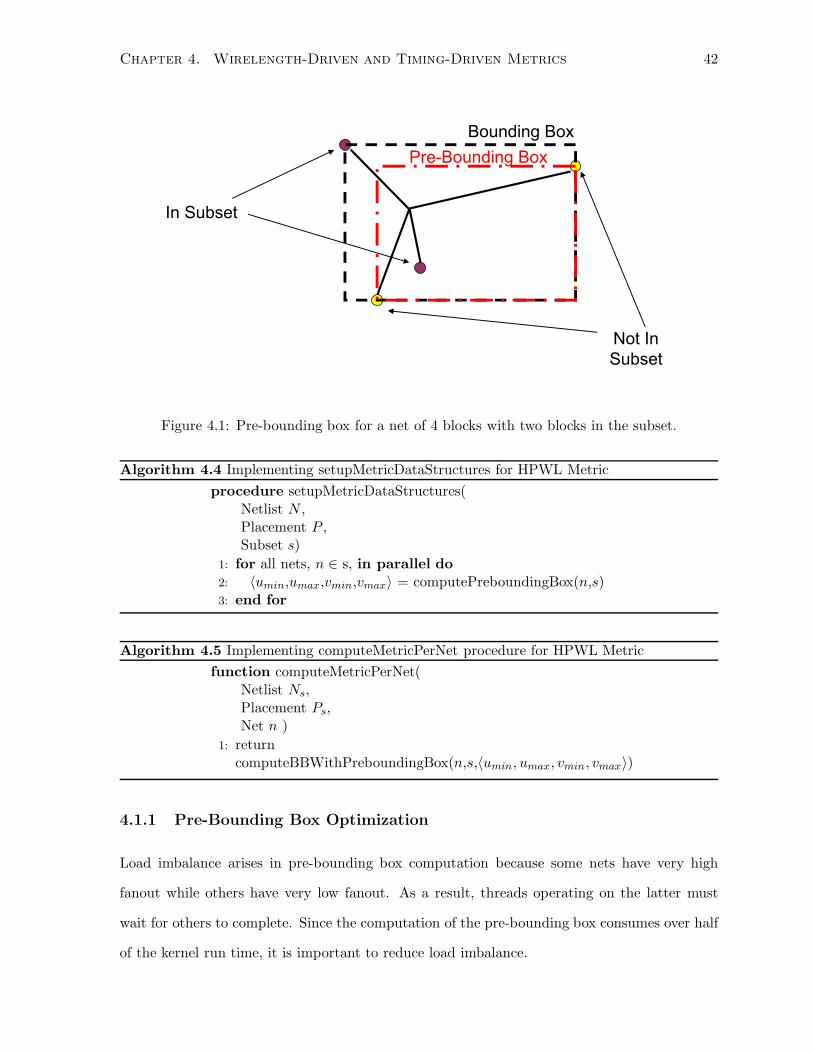
Chapter 4. Wirelength-Driven and Timing-Driven Metrics 42
In Subset
Not In
Subset
Bounding Box
Pre-Bounding Box
Figure 4.1: Pre-bounding box for a net of 4 blocks with two blocks in the subset.
Algorithm 4.4 Implementing setupMetricDataStructures for HPWL Metric
procedure setupMetricDataStructures(Netlist N ,Placement P ,Subset s)
1: for all nets, n ∈ s, in parallel do2: 〈umin,umax,vmin,vmax〉 = computePreboundingBox(n,s)3: end for
Algorithm 4.5 Implementing computeMetricPerNet procedure for HPWL Metric
function computeMetricPerNet(Netlist Ns,Placement Ps,Net n )
1: returncomputeBBWithPreboundingBox(n,s,〈umin, umax, vmin, vmax〉)
4.1.1 Pre-Bounding Box Optimization
Load imbalance arises in pre-bounding box computation because some nets have very high
fanout while others have very low fanout. As a result, threads operating on the latter must
wait for others to complete. Since the computation of the pre-bounding box consumes over half
of the kernel run time, it is important to reduce load imbalance.
Chapter 4. Wirelength-Driven and Timing-Driven Metrics 43
To alleviate this problem, if the fanout of a net is too high, a random subset of P blocks
on the subject net is used to compute the pre-bounding box. For the current implementation,
P = 8. While this may introduce inaccuracies, it significantly helps in runtime. In particular,
benchmarks with many high-fanout nets will suffer from this approximation. We found that
using only eight blocks was sufficient to maintain quality for most of the benchmarks, despite the
presence of nets with fanout greater than one hundred. Thus the maximum number of blocks
used in a pre-bounding box computation becomes a tunable parameter to trade-off between
quality and performance. It should be mentioned that while P = 8 is sufficient for the purposes
of the given benchmarks, this may not be true for other benchmarks.
4.2 Challenges with Timing-Driven Placement using GPGPU
The next objective is to extend the wirelength-driven placement framework so that it is also
timing-driven.
4.2.1 Challenge with VPR’s Metric
An obvious choice for a timing metric is VPR’s metric which is net-based [5]. Unfortunately, this
metric consumes precious shared memory resources. The metric focuses on edges in the netlist,
which are point-to-point connections which connect a source block to a sink block. Greater
emphasis is placed on minimizing edges which are critical. The metric is given in Section 2.1
as Equation 2.3.
This metric is different from the wirelength-driven metric since the wirelength metric focuses
on nets and the timing metric focuses on edges. A net has a single source and one or more sinks,
while an edge has exactly one source and one sink. Thus for each net, there can be multiple
edges.
Shared Memory Requirement An concrete is example is given of the required memory
for the HPWL metric. For each block, 12 bytes of memory are used, and for
each net 22 bytes are used by the implementation of the wirelength metric. In
addition there are 384 bytes used for bookkeeping. The shared memory usage,
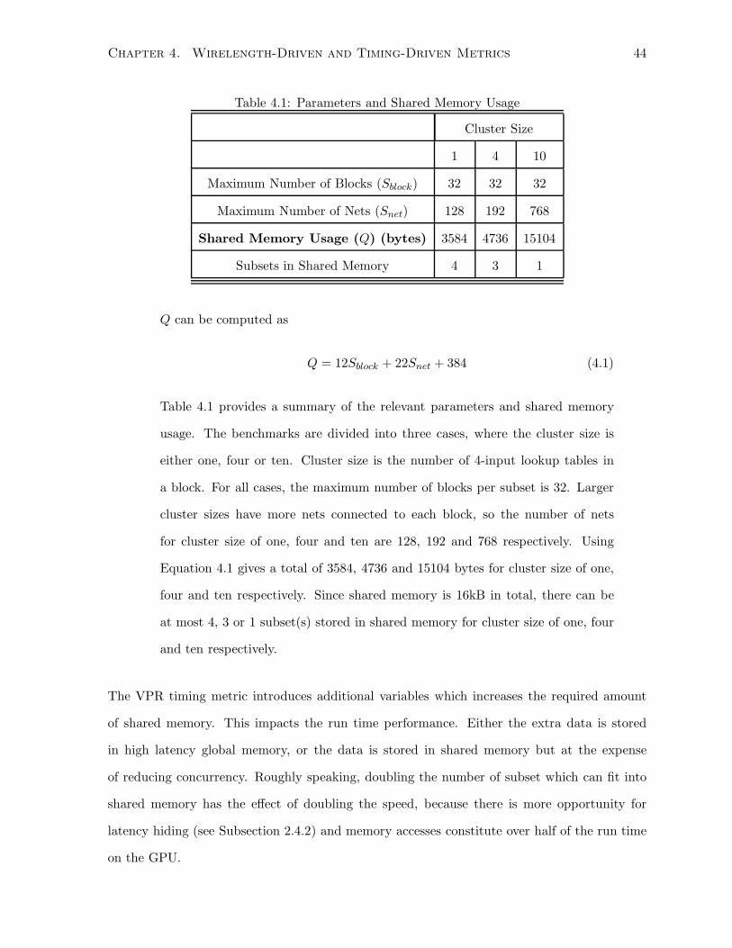
Chapter 4. Wirelength-Driven and Timing-Driven Metrics 44
Table 4.1: Parameters and Shared Memory Usage
Cluster Size
1 4 10
Maximum Number of Blocks (Sblock) 32 32 32
Maximum Number of Nets (Snet) 128 192 768
Shared Memory Usage (Q) (bytes) 3584 4736 15104
Subsets in Shared Memory 4 3 1
Q can be computed as
Q = 12Sblock + 22Snet + 384 (4.1)
Table 4.1 provides a summary of the relevant parameters and shared memory
usage. The benchmarks are divided into three cases, where the cluster size is
either one, four or ten. Cluster size is the number of 4-input lookup tables in
a block. For all cases, the maximum number of blocks per subset is 32. Larger
cluster sizes have more nets connected to each block, so the number of nets
for cluster size of one, four and ten are 128, 192 and 768 respectively. Using
Equation 4.1 gives a total of 3584, 4736 and 15104 bytes for cluster size of one,
four and ten respectively. Since shared memory is 16kB in total, there can be
at most 4, 3 or 1 subset(s) stored in shared memory for cluster size of one, four
and ten respectively.
The VPR timing metric introduces additional variables which increases the required amount
of shared memory. This impacts the run time performance. Either the extra data is stored
in high latency global memory, or the data is stored in shared memory but at the expense
of reducing concurrency. Roughly speaking, doubling the number of subset which can fit into
shared memory has the effect of doubling the speed, because there is more opportunity for
latency hiding (see Subsection 2.4.2) and memory accesses constitute over half of the run time
on the GPU.
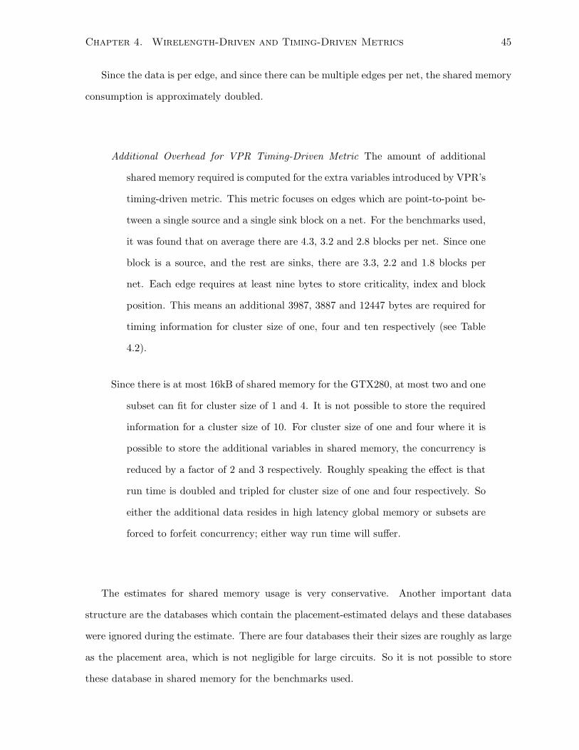
Chapter 4. Wirelength-Driven and Timing-Driven Metrics 45
Since the data is per edge, and since there can be multiple edges per net, the shared memory
consumption is approximately doubled.
Additional Overhead for VPR Timing-Driven Metric The amount of additional
shared memory required is computed for the extra variables introduced by VPR’s
timing-driven metric. This metric focuses on edges which are point-to-point be-
tween a single source and a single sink block on a net. For the benchmarks used,
it was found that on average there are 4.3, 3.2 and 2.8 blocks per net. Since one
block is a source, and the rest are sinks, there are 3.3, 2.2 and 1.8 blocks per
net. Each edge requires at least nine bytes to store criticality, index and block
position. This means an additional 3987, 3887 and 12447 bytes are required for
timing information for cluster size of one, four and ten respectively (see Table
4.2).
Since there is at most 16kB of shared memory for the GTX280, at most two and one
subset can fit for cluster size of 1 and 4. It is not possible to store the required
information for a cluster size of 10. For cluster size of one and four where it is
possible to store the additional variables in shared memory, the concurrency is
reduced by a factor of 2 and 3 respectively. Roughly speaking the effect is that
run time is doubled and tripled for cluster size of one and four respectively. So
either the additional data resides in high latency global memory or subsets are
forced to forfeit concurrency; either way run time will suffer.
The estimates for shared memory usage is very conservative. Another important data
structure are the databases which contain the placement-estimated delays and these databases
were ignored during the estimate. There are four databases their their sizes are roughly as large
as the placement area, which is not negligible for large circuits. So it is not possible to store
these database in shared memory for the benchmarks used.
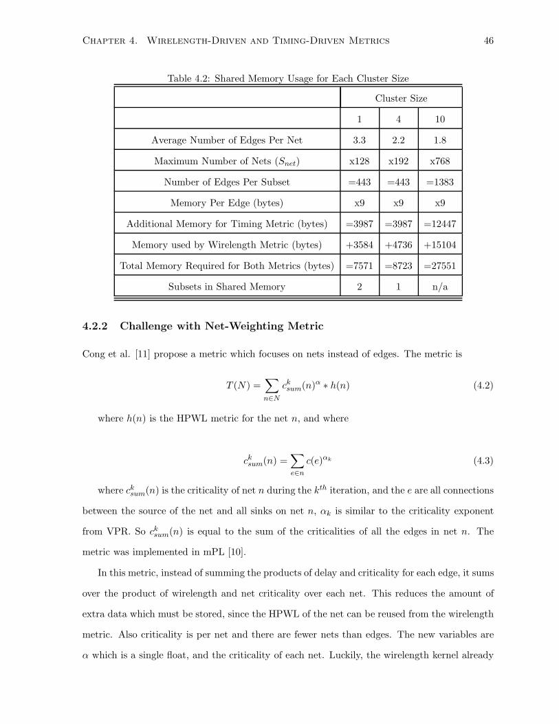
Chapter 4. Wirelength-Driven and Timing-Driven Metrics 46
Table 4.2: Shared Memory Usage for Each Cluster Size
Cluster Size
1 4 10
Average Number of Edges Per Net 3.3 2.2 1.8
Maximum Number of Nets (Snet) x128 x192 x768
Number of Edges Per Subset =443 =443 =1383
Memory Per Edge (bytes) x9 x9 x9
Additional Memory for Timing Metric (bytes) =3987 =3987 =12447
Memory used by Wirelength Metric (bytes) +3584 +4736 +15104
Total Memory Required for Both Metrics (bytes) =7571 =8723 =27551
Subsets in Shared Memory 2 1 n/a
4.2.2 Challenge with Net-Weighting Metric
Cong et al. [11] propose a metric which focuses on nets instead of edges. The metric is
T (N) =∑
n∈N
cksum(n)α ∗ h(n) (4.2)
where h(n) is the HPWL metric for the net n, and where
cksum(n) =
∑
e∈n
c(e)αk (4.3)
where cksum(n) is the criticality of net n during the kth iteration, and the e are all connections
between the source of the net and all sinks on net n, αk is similar to the criticality exponent
from VPR. So cksum(n) is equal to the sum of the criticalities of all the edges in net n. The
metric was implemented in mPL [10].
In this metric, instead of summing the products of delay and criticality for each edge, it sums
over the product of wirelength and net criticality over each net. This reduces the amount of
extra data which must be stored, since the HPWL of the net can be reused from the wirelength
metric. Also criticality is per net and there are fewer nets than edges. The new variables are
α which is a single float, and the criticality of each net. Luckily, the wirelength kernel already
Chapter 4. Wirelength-Driven and Timing-Driven Metrics 47
allocates a region of shared memory which can accommodate the net criticality, and which is
not used during the annealing processes.1 Therefore no additional shared memory is used for
this metric except for the extra float for α.
Unfortunately, the metric does not always produce results which are of the same quality as
VPR (Table 4.3). The table gives the ratio of the average critical path delay from the proposed
metric to standard VPR, so values greater than one indicate that the new metric is worse. The
average is taken over five different seeds. On average results are within 3% of the VPR metric.
However, there are some cases which are better, such as b19 1 and b19 (cluster size of one),
and some worse, such as b18 (cluster size of one). On average, Cong’s metric is 3.6%, 3.7% and
1.7% worse for cluster size of one, four and ten, which are all within their respective standard
deviations.
4.2.3 Resolving Challenges
The ideal solution would have low shared memory usage while producing high quality placement
results.
4.2.4 Investigating Sum Operator
Intuitively, it seems that the summation operator overestimates the criticality for a net. For
instance if a net contains many low critical critical edges, then its criticality value can be be
greater than a net with a single high critical value. This incorrectly places more emphasis on
high fanout nets which may not need to be optimized.
To investigate this problem, the addition operator is replaced with a maximum operator.
So the criticality is computed as follows
ckmax(e) = max
e∈n(c(e)αk ) (4.4)
This the metric should reduce the amount of overestimation. Results are given for the
maximum operator in Table 4.4). For these results, the ratio is between the average critical
1This region is only used during the setup portion of the kernel. Unfortunately, the CUDA API does notallow for shared memory to be dynamically allocated and freed, so that region would otherwise be unused.
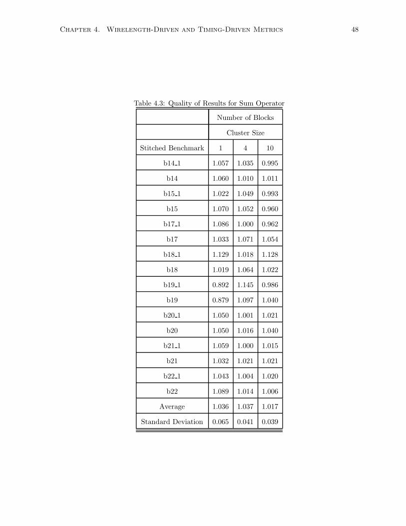
Chapter 4. Wirelength-Driven and Timing-Driven Metrics 48
Table 4.3: Quality of Results for Sum Operator
Number of Blocks
Cluster Size
Stitched Benchmark 1 4 10
b14 1 1.057 1.035 0.995
b14 1.060 1.010 1.011
b15 1 1.022 1.049 0.993
b15 1.070 1.052 0.960
b17 1 1.086 1.000 0.962
b17 1.033 1.071 1.054
b18 1 1.129 1.018 1.128
b18 1.019 1.064 1.022
b19 1 0.892 1.145 0.986
b19 0.879 1.097 1.040
b20 1 1.050 1.001 1.021
b20 1.050 1.016 1.040
b21 1 1.059 1.000 1.015
b21 1.032 1.021 1.021
b22 1 1.043 1.004 1.020
b22 1.089 1.014 1.006
Average 1.036 1.037 1.017
Standard Deviation 0.065 0.041 0.039
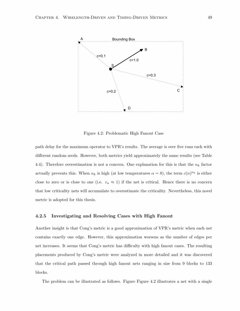
Chapter 4. Wirelength-Driven and Timing-Driven Metrics 49
Bounding Box
c=1.0
c=0.3
c=0.2
c=0.1
C
S
A
B
D
Figure 4.2: Problematic High Fanout Case
path delay for the maximum operator to VPR’s results. The average is over five runs each with
different random seeds. However, both metrics yield approximately the same results (see Table
4.4). Therefore overestimation is not a concern. One explanation for this is that the αk factor
actually prevents this. When αk is high (at low temperatures α = 8), the term c(n)αk is either
close to zero or is close to one (i.e. cn ≈ 1) if the net is critical. Hence there is no concern
that low criticality nets will accumulate to overestimate the criticality. Nevertheless, this novel
metric is adopted for this thesis.
4.2.5 Investigating and Resolving Cases with High Fanout
Another insight is that Cong’s metric is a good approximation of VPR’s metric when each net
contains exactly one edge. However, this approximation worsens as the number of edges per
net increases. It seems that Cong’s metric has difficulty with high fanout cases. The resulting
placements produced by Cong’s metric were analyzed in more detailed and it was discovered
that the critical path passed through high fanout nets ranging in size from 9 blocks to 133
blocks.
The problem can be illustrated as follows. Figure Figure 4.2 illustrates a net with a single
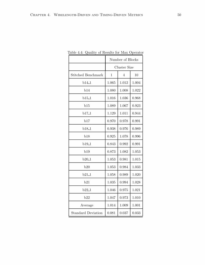
Chapter 4. Wirelength-Driven and Timing-Driven Metrics 50
Table 4.4: Quality of Results for Max Operator
Number of Blocks
Cluster Size
Stitched Benchmark 1 4 10
b14 1 1.065 1.012 1.004
b14 1.080 1.008 1.022
b15 1 1.016 1.036 0.968
b15 1.089 1.067 0.923
b17 1 1.129 1.011 0.944
b17 0.970 0.978 0.991
b18 1 0.938 0.976 0.989
b18 0.925 1.078 0.996
b19 1 0.843 0.992 0.991
b19 0.873 1.082 1.053
b20 1 1.053 0.981 1.015
b20 1.053 0.984 1.033
b21 1 1.058 0.989 1.020
b21 1.035 0.994 1.028
b22 1 1.046 0.975 1.021
b22 1.047 0.973 1.010
Average 1.014 1.009 1.001
Standard Deviation 0.081 0.037 0.033
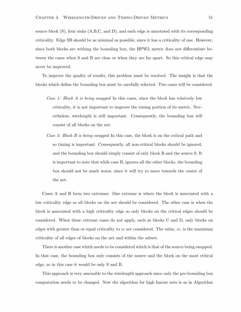
Chapter 4. Wirelength-Driven and Timing-Driven Metrics 51
source block (S), four sinks (A,B,C, and D), and each edge is annotated with its corresponding
criticality. Edge SB should be as minimal as possible, since it has a criticality of one. However,
since both blocks are withing the bounding box, the HPWL metric does not differentiate be-
tween the cases when S and B are close or when they are far apart. So this critical edge may
never be improved.
To improve the quality of results, this problem must be resolved. The insight is that the
blocks which define the bounding box must be carefully selected. Two cases will be considered.
Case 1: Block A is being swapped In this cases, since the block has relatively low
criticality, it is not important to improve the timing portion of its metric. Nev-
ertheless, wirelength is still important. Consequently, the bounding box will
consist of all blocks on the net.
Case 2: Block B is being swapped In this case, the block is on the critical path and
so timing is important. Consequently, all non-critical blocks should be ignored,
and the bounding box should simply consist of only block B and the source S. It
is important to note that while case B, ignores all the other blocks, the bounding
box should not be much worse, since it will try to move towards the center of
the net.
Cases A and B form two extremes. One extreme is where the block is associated with a
low criticality edge so all blocks on the net should be considered. The other case is when the
block is associated with a high criticality edge so only blocks on the critical edges should be
considered. When these extreme cases do not apply, such as blocks C and D, only blocks on
edges with greater than or equal criticality to cc are considered. The value, cc, is the maximum
criticality of all edges of blocks on the net and within the subset.
There is another case which needs to be considered which is that of the source being swapped.
In that case, the bounding box only consists of the source and the block on the most critical
edge, so in this case it would be only S and B.
This approach is very amenable to the wirelength approach since only the pre-bounding box
computation needs to be changed. Now the algorithm for high fanout nets is as in Algorithm
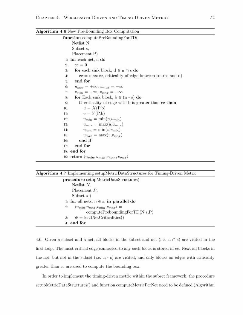
Chapter 4. Wirelength-Driven and Timing-Driven Metrics 52
Algorithm 4.6 New Pre-Bounding Box Computation
function computePreBoundingForTD(Netlist N,Subset s,Placement P)
1: for each net, n do2: cc = 03: for each sink block, d ∈ n ∩ s do4: cc = max(cc, criticality of edge between source and d)5: end for6: umin = +∞, umax = −∞7: vmin = +∞, vmax = −∞8: for Each sink block, b ∈ (n - s) do9: if criticality of edge with b is greater than cc then
10: u = X(P,b)11: v = Y (P,b)12: umin = min(u,umin)13: umax = max(u,umax)14: vmin = min(v,vmin)15: vmax = max(v,vmax)16: end if17: end for18: end for19: return 〈umin, umax, vmin, vmax〉
Algorithm 4.7 Implementing setupMetricDataStructures for Timing-Driven Metric
procedure setupMetricDataStructures(Netlist N ,Placement P ,Subset s )
1: for all nets, n ∈ s, in parallel do2: 〈umin,umax,vmin,vmax〉 =
computePreboundingForTD(N,s,P)3: w = loadNetCriticalities()4: end for
4.6. Given a subset and a net, all blocks in the subset and net (i.e. n ∩ s) are visited in the
first loop. The most critical edge connected to any such block is stored in cc. Next all blocks in
the net, but not in the subset (i.e. n - s) are visited, and only blocks on edges with criticality
greater than cc are used to compute the bounding box.
In order to implement the timing-driven metric within the subset framework, the procedure
setupMetricDataStructures() and function computeMetricPerNet need to be defined (Algorithm
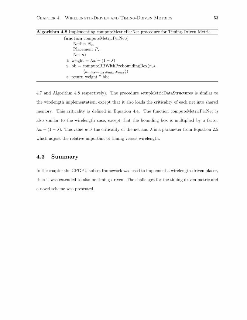
Chapter 4. Wirelength-Driven and Timing-Driven Metrics 53
Algorithm 4.8 Implementing computeMetricPerNet procedure for Timing-Driven Metric
function computeMetricPerNet(Netlist Ns,Placement Ps,Net n)
1: weight = λw + (1 − λ)2: bb = computeBBWithPreboundingBox(n,s,
〈umin,umax,vmin,vmax〉)3: return weight * bb;
4.7 and Algorithm 4.8 respectively). The procedure setupMetricDataStructures is similar to
the wirelength implementation, except that it also loads the criticality of each net into shared
memory. This criticality is defined in Equation 4.4. The function computeMetricPerNet is
also similar to the wirelength case, except that the bounding box is multiplied by a factor
λw + (1 − λ). The value w is the criticality of the net and λ is a parameter from Equation 2.5
which adjust the relative important of timing versus wirelength.
4.3 Summary
In the chapter the GPGPU subset framework was used to implement a wirelength-driven placer,
then it was extended to also be timing-driven. The challenges for the timing-driven metric and
a novel scheme was presented.
Chapter 5
Evaluation and Analysis
This chapter compares the subset-based framework to a sequential implementation in terms of
quality of results and run time, then it analyzes the overall behavior of the framework.
5.1 Evaluation Methodology
This section aims to describe the methodology in sufficient detail such that it can be reproduced
and critiqued.
5.1.1 Benchmarks
A challenge in evaluating placement scalability and quality of results is the lack of large academic
circuits for FPGAs. To obtain a set of large benchmarks, the benchmarks from the ITC99 suite
were increased in size using a technique devised at Altera [1]. Each benchmark core is replicated
10 times and then primary input and output pins are connected together via long shift registers
as described in Altera’s literature and a previous work[1, 7]. In addition, the number of primary
inputs and outputs is increased such that it adheres to Rent’s rule with a Rent exponent of
0.5 and constant of 1.0 (e.g. a circuit with 100K LUTs would have (105)0.5 = 316 inputs and
outputs [22]). This is accomplished by taking input or output pins for the replicated cores
which are internally connect to long shift registers and instead making them primary inputs or
outputs.
54
Chapter 5. Evaluation and Analysis 55
The sizes of each benchmark are given in Table 5.1. They were clustered using T-VPACK
[5] using cluster sizes of one, four and ten. The cluster size is the number of 4-input lookup
tables per block.
5.1.2 Sequential Simulated Annealing Placer
The GPGPU implementation is compared against VPR 4.3 in fast mode which performs ten
times fewer annealing moves than the default. All other settings are left as default. The default
for VPR is to place equal weighting on the timing and wirelength metrics, so λ = 0.5 for Equa-
tion 2.5. The architectural file used was the one provided in VPR 4.3 (4x4lut sanitized.arch)
which uses four 4-input lookup tables per block. Additional architectural files were generated
from this file to support cluster sizes of 1 and 10.
VPR uses a more sophisticated metric for wirelength, which is
Hvpr =∑
n∈N
q(n)(hx(n)/cx(n) + hy(n)/cy(n)) (5.1)
where (hx(n) and hy(n) are the length of the bounding box in the x and y directions, cx(n)
and cy(n) are the congestion in the x and y direction, and q(n) is a correction factor for high
fanout nets and N is the set of all nets[5]. For this work, this metric is not used, but instead
the simple HPWL metric (see Equation 2.2). For the sake of experimentation, VPR has been
modified to use this metric.
5.1.3 Hardware Setup
The proposed framework is implemented using the C++ language and CUDA, which is NVIDIA’s
framework for writing C code for their GPUs. Both the sequential and parallel version were
executed on a Intel (R) Core (TM) 2 Quad (at 2.66 GHz) as the CPU with 2GB of RAM and
NVIDIA’s GTX280 (at 1.35 GHz) as the GPU, with 1GB of RAM. Later on results are given
for the GTX480 with a clock frequency of 1.40 GHz and 1.5GB of RAM. Only one of the four
cores was used for all experiments. All binaries are compiled with the highest optimization
level.
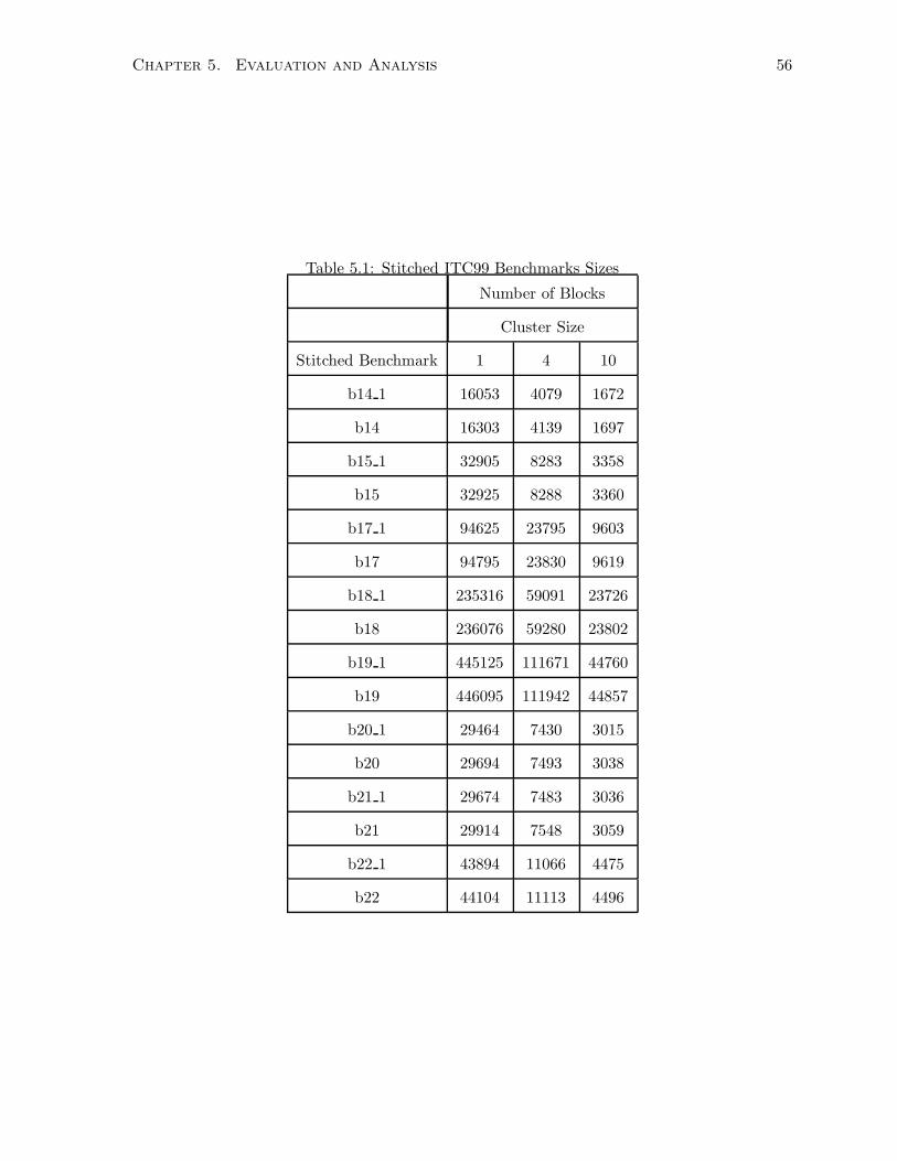
Chapter 5. Evaluation and Analysis 56
Table 5.1: Stitched ITC99 Benchmarks Sizes
Number of Blocks
Cluster Size
Stitched Benchmark 1 4 10
b14 1 16053 4079 1672
b14 16303 4139 1697
b15 1 32905 8283 3358
b15 32925 8288 3360
b17 1 94625 23795 9603
b17 94795 23830 9619
b18 1 235316 59091 23726
b18 236076 59280 23802
b19 1 445125 111671 44760
b19 446095 111942 44857
b20 1 29464 7430 3015
b20 29694 7493 3038
b21 1 29674 7483 3036
b21 29914 7548 3059
b22 1 43894 11066 4475
b22 44104 11113 4496
Chapter 5. Evaluation and Analysis 57
5.2 Parameters for GPGPU Framework
In order to implement the subset-based framework, several parameters have to be selected which
impact run time and quality of results. Each of the parameters are discussed below. The values
for parameters are given in Table 5.3 unless it was being varied. Quality of results is the ratio
of the GPU results to sequential, so less than one is better. Speedup is the ratio of the run time
of the sequential to the GPU one. As a side note, runs of the sequential version with different
random seeds have an standard devivation of 2%, 0.6% and 0.8% for cluster size of one, four
and ten respectively. Any results within the standard deviation are assumed to be sufficiently
close to the sequential results. The results are averaged across b14, b15, b20, b21 and b22 and
the wirelength metric is used.
Most of the parameters are independent, except for the number of subsets and subset
size, because these two parameters directly impact the amount of shared memory, and shared
memory is limited. So either many small subsets can be annealed or several large subsets can
be annealed.
Number of Subsets (Ns): The number of subsets is how many subsets are annealed
concurrently, Increasing the number of subsets running concurrently should improve run time
up to the point where the GPU resources are fully utilized. At the same time, increasing the
number of subsets should not impact quality as long as the netlist is large enough. Since the
GTX280 has 30 SMPs, a multiple of 30 SMPs should be used to avoid idle SMPs.
From Figure 5.1 (a), the speedup has a very interesting behavior depending on the cluster
size. For cluster size of 10, the speedup decreases with the number of subsets, this is because
the GPU is saturated at thirty subsets. As the number of subsets increases, the time spent
annealing the subset on the GPU is fixed. However, the time spent on generating the additional
subsets increases, and causes stall because the GPU must wait longer for the CPU to generate
the subsets. This effect could be mitigated by increasing reuse.
For cluster size of 4, the speedup increases with more subsets because the GPU can con-
currently anneal the extra subsets. Once the number of subsets increases beyond the GPUs
capacity (which is 90 concurrent subsets), the speedup worses for the same reason as cluster
Chapter 5. Evaluation and Analysis 58
size of ten. For cluster size of 1, a similar trend is seen.
Figure 5.1 (b) gives the impact on quality of results. In terms of quality, for cluster size of
1 and 4 the degradation is within the standard deviation. For cluster size of 10 (and also for
4), the quality worses as the number of subsets approaches 300. At this point, there are not
enough blocks within the netlist to create that many subsets. Thus parallelism is limited by
the size of the netlist. This is not a concern, since netlists are expected to increase in size with
each new generate of FPGA devices.
Subset Size (Ss): The subset size is the number of blocks in the subset. Adjusting the
size of the subset should not significantly impact run time since the time required to generate
and anneal a subset is proportional to its size. Quality should not be affected directly by subset
size. Instead it should be affected by the number of moves per blocks within a subset and this
parameter will be shortly discussed.
For this experiment, the number of moves per subset equaled half the subset size (so 14
moves would be performed on a subset of 28 blocks). As expected the speedup is not affected
significantly by changing the subset size (Figure 5.2(a)). When the subset size is small (between
12-16 blocks) the hardware resources are not fully utilized, so speedup is less in these cases.
Speedup increases as the subset increases in size and the hardware resources are better utilized.
The quality of results vary by less than 2%, which is attributed to random fluctuations, so there
is virtual no impact on quality of results (Figure 5.2(b)).
Number of moves per subset (M): This parameter is a trade off between run time
and quality of results. Increasing the number of moves per subset amortizes the time spent on
loading data from global memory to shared memory, but this causes move bias which degrades
quality of results (see Subsection 3.3.1). Looking at the results from Figure 5.3, increasing the
number of moves tends to improve speedup at the cost of degrading quality as expected.
Reuse: Reuse describes the average number of times a subset group will be used, where a
subset group is a collection of subsets which can be annealed on the GPU. When a subset group
is reused, the computation otherwise required for generating a subset is saved and this prevents
the CPU from otherwise being the bottleneck. The drawback is that each time a subset is
reused it biases the moves within the subset which could worsen quality.
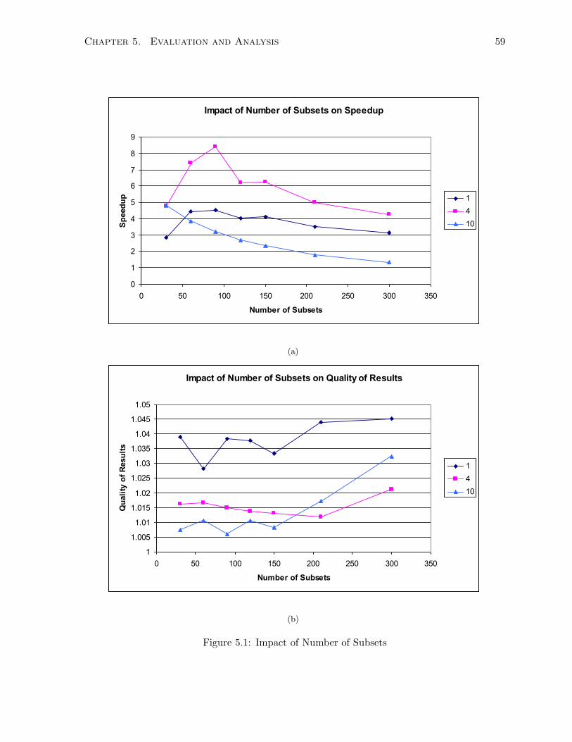
Chapter 5. Evaluation and Analysis 59
Impact of Number of Subsets on Speedup
0
1
2
3
4
5
6
7
8
9
0 50 100 150 200 250 300 350
Number of Subsets
Sp
eed
up 1
4
10
(a)
Impact of Number of Subsets on Quality of Results
1
1.005
1.01
1.015
1.02
1.025
1.03
1.035
1.04
1.045
1.05
0 50 100 150 200 250 300 350
Number of Subsets
Qu
ali
ty o
f R
esu
lts
1
4
10
(b)
Figure 5.1: Impact of Number of Subsets
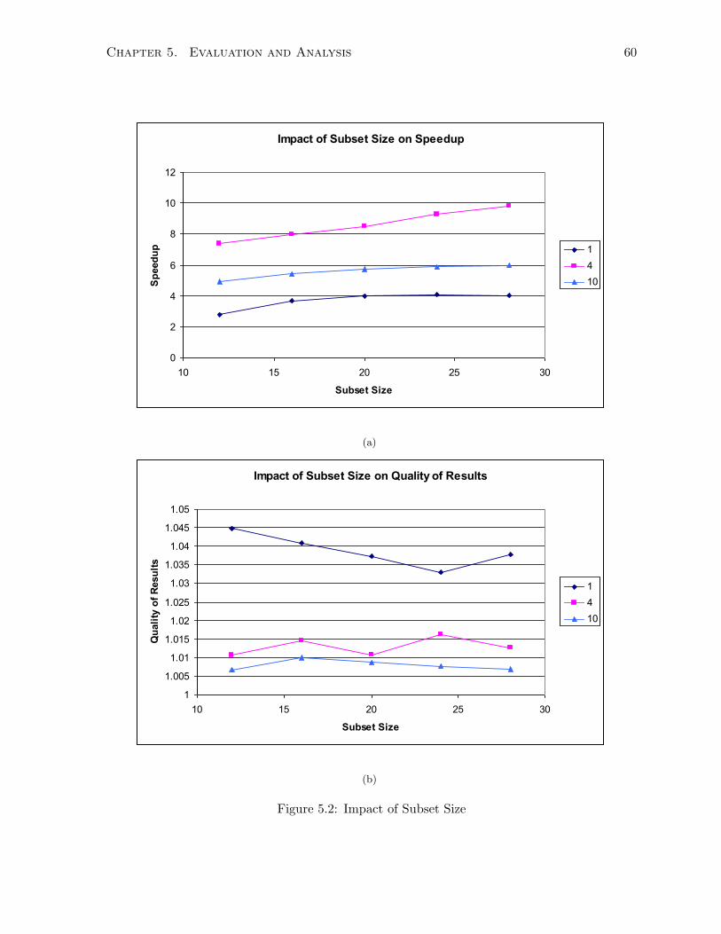
Chapter 5. Evaluation and Analysis 60
Impact of Subset Size on Speedup
0
2
4
6
8
10
12
10 15 20 25 30
Subset Size
Sp
eed
up 1
4
10
(a)
Impact of Subset Size on Quality of Results
1
1.005
1.01
1.015
1.02
1.025
1.03
1.035
1.04
1.045
1.05
10 15 20 25 30
Subset Size
Qu
ali
ty o
f R
esu
lts
1
4
10
(b)
Figure 5.2: Impact of Subset Size
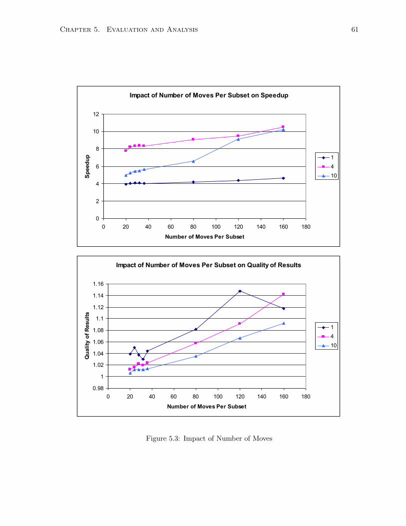
Chapter 5. Evaluation and Analysis 61
Impact of Number of Moves Per Subset on Speedup
0
2
4
6
8
10
12
0 20 40 60 80 100 120 140 160 180
Number of Moves Per Subset
Sp
eed
up 1
4
10
Impact of Number of Moves Per Subset on Quality of Results
0.98
1
1.02
1.04
1.06
1.08
1.1
1.12
1.14
1.16
0 20 40 60 80 100 120 140 160 180
Number of Moves Per Subset
Qu
ali
ty o
f R
esu
lts
1
4
10
Figure 5.3: Impact of Number of Moves
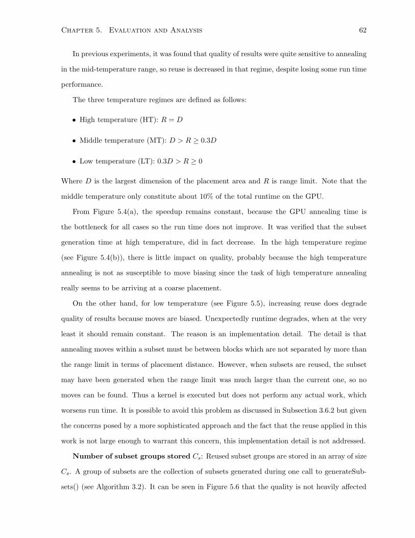
Chapter 5. Evaluation and Analysis 62
In previous experiments, it was found that quality of results were quite sensitive to annealing
in the mid-temperature range, so reuse is decreased in that regime, despite losing some run time
performance.
The three temperature regimes are defined as follows:
• High temperature (HT): R = D
• Middle temperature (MT): D > R ≥ 0.3D
• Low temperature (LT): 0.3D > R ≥ 0
Where D is the largest dimension of the placement area and R is range limit. Note that the
middle temperature only constitute about 10% of the total runtime on the GPU.
From Figure 5.4(a), the speedup remains constant, because the GPU annealing time is
the bottleneck for all cases so the run time does not improve. It was verified that the subset
generation time at high temperature, did in fact decrease. In the high temperature regime
(see Figure 5.4(b)), there is little impact on quality, probably because the high temperature
annealing is not as susceptible to move biasing since the task of high temperature annealing
really seems to be arriving at a coarse placement.
On the other hand, for low temperature (see Figure 5.5), increasing reuse does degrade
quality of results because moves are biased. Unexpectedly runtime degrades, when at the very
least it should remain constant. The reason is an implementation detail. The detail is that
annealing moves within a subset must be between blocks which are not separated by more than
the range limit in terms of placement distance. However, when subsets are reused, the subset
may have been generated when the range limit was much larger than the current one, so no
moves can be found. Thus a kernel is executed but does not perform any actual work, which
worsens run time. It is possible to avoid this problem as discussed in Subsection 3.6.2 but given
the concerns posed by a more sophisticated approach and the fact that the reuse applied in this
work is not large enough to warrant this concern, this implementation detail is not addressed.
Number of subset groups stored Cs: Reused subset groups are stored in an array of size
Cs. A group of subsets are the collection of subsets generated during one call to generateSub-
sets() (see Algorithm 3.2). It can be seen in Figure 5.6 that the quality is not heavily affected
Chapter 5. Evaluation and Analysis 63
Impact of High Temperature Reuse on Speedup
0
1
2
3
4
5
6
7
8
0 5 10 15 20 25 30 35
High Temperature Reuse
Sp
eed
up 1
4
10
(a)
Impact of High Temperature Reuse on Quality of Results
1
1.005
1.01
1.015
1.02
1.025
1.03
1.035
1.04
1.045
1.05
0 5 10 15 20 25 30 35
High Temperature Reuse
Qu
ali
ty o
f R
esu
lts
1
4
10
(b)
Figure 5.4: Impact of High Temperature Reuse
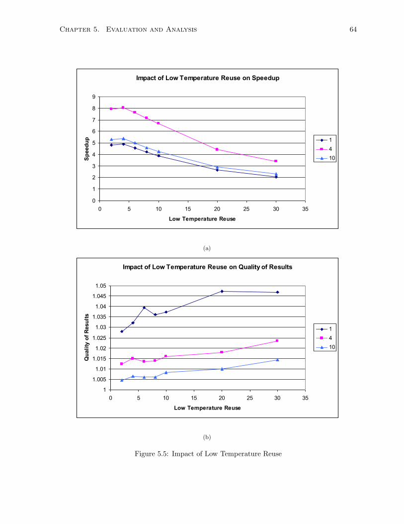
Chapter 5. Evaluation and Analysis 64
Impact of Low Temperature Reuse on Speedup
0
1
2
3
4
5
6
7
8
9
0 5 10 15 20 25 30 35
Low Temperature Reuse
Sp
eed
up 1
4
10
(a)
Impact of Low Temperature Reuse on Quality of Results
1
1.005
1.01
1.015
1.02
1.025
1.03
1.035
1.04
1.045
1.05
0 5 10 15 20 25 30 35
Low Temperature Reuse
Qu
ali
ty o
f R
esu
lts
1
4
10
(b)
Figure 5.5: Impact of Low Temperature Reuse
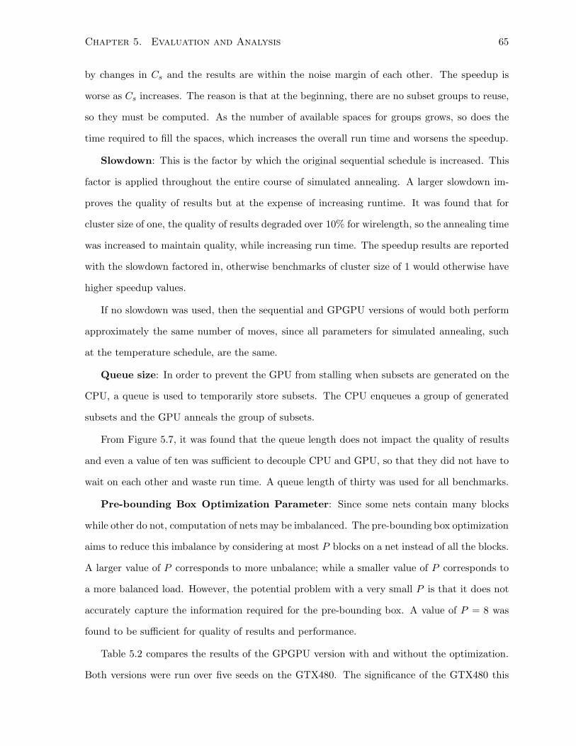
Chapter 5. Evaluation and Analysis 65
by changes in Cs and the results are within the noise margin of each other. The speedup is
worse as Cs increases. The reason is that at the beginning, there are no subset groups to reuse,
so they must be computed. As the number of available spaces for groups grows, so does the
time required to fill the spaces, which increases the overall run time and worsens the speedup.
Slowdown: This is the factor by which the original sequential schedule is increased. This
factor is applied throughout the entire course of simulated annealing. A larger slowdown im-
proves the quality of results but at the expense of increasing runtime. It was found that for
cluster size of one, the quality of results degraded over 10% for wirelength, so the annealing time
was increased to maintain quality, while increasing run time. The speedup results are reported
with the slowdown factored in, otherwise benchmarks of cluster size of 1 would otherwise have
higher speedup values.
If no slowdown was used, then the sequential and GPGPU versions of would both perform
approximately the same number of moves, since all parameters for simulated annealing, such
at the temperature schedule, are the same.
Queue size: In order to prevent the GPU from stalling when subsets are generated on the
CPU, a queue is used to temporarily store subsets. The CPU enqueues a group of generated
subsets and the GPU anneals the group of subsets.
From Figure 5.7, it was found that the queue length does not impact the quality of results
and even a value of ten was sufficient to decouple CPU and GPU, so that they did not have to
wait on each other and waste run time. A queue length of thirty was used for all benchmarks.
Pre-bounding Box Optimization Parameter: Since some nets contain many blocks
while other do not, computation of nets may be imbalanced. The pre-bounding box optimization
aims to reduce this imbalance by considering at most P blocks on a net instead of all the blocks.
A larger value of P corresponds to more unbalance; while a smaller value of P corresponds to
a more balanced load. However, the potential problem with a very small P is that it does not
accurately capture the information required for the pre-bounding box. A value of P = 8 was
found to be sufficient for quality of results and performance.
Table 5.2 compares the results of the GPGPU version with and without the optimization.
Both versions were run over five seeds on the GTX480. The significance of the GTX480 this
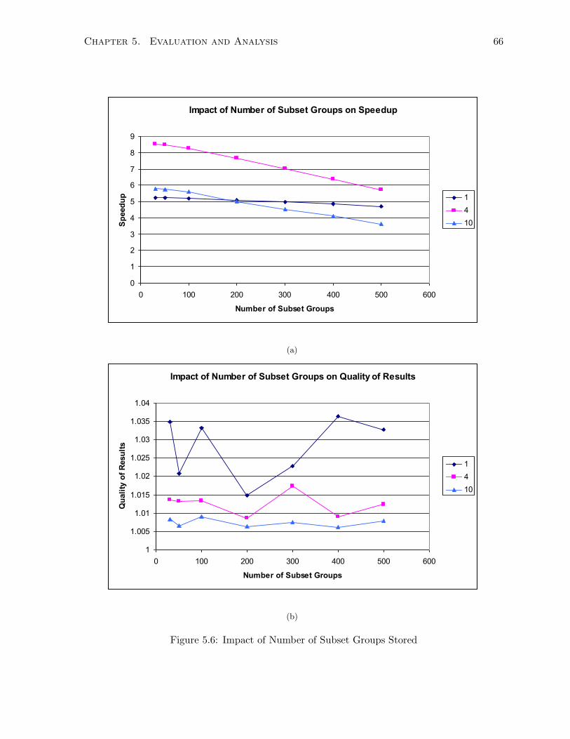
Chapter 5. Evaluation and Analysis 66
Impact of Number of Subset Groups on Speedup
0
1
2
3
4
5
6
7
8
9
0 100 200 300 400 500 600
Number of Subset Groups
Sp
eed
up 1
4
10
(a)
Impact of Number of Subset Groups on Quality of Results
1
1.005
1.01
1.015
1.02
1.025
1.03
1.035
1.04
0 100 200 300 400 500 600
Number of Subset Groups
Qu
ali
ty o
f R
esu
lts
1
4
10
(b)
Figure 5.6: Impact of Number of Subset Groups Stored
Chapter 5. Evaluation and Analysis 67
Impact of Queue Size on Speedup
0
1
2
3
4
5
6
7
8
0 10 20 30 40 50 60 70 80 90
Queue Size
Sp
eed
up 1
4
10
(a)
Impact of Queue Size on Quality of Results
1
1.005
1.01
1.015
1.02
1.025
1.03
1.035
1.04
1.045
1.05
0 10 20 30 40 50 60 70 80 90
Queue Size
Qu
ali
ty o
f R
esu
lts
1
4
10
(b)
Figure 5.7: Impact of Queue Size
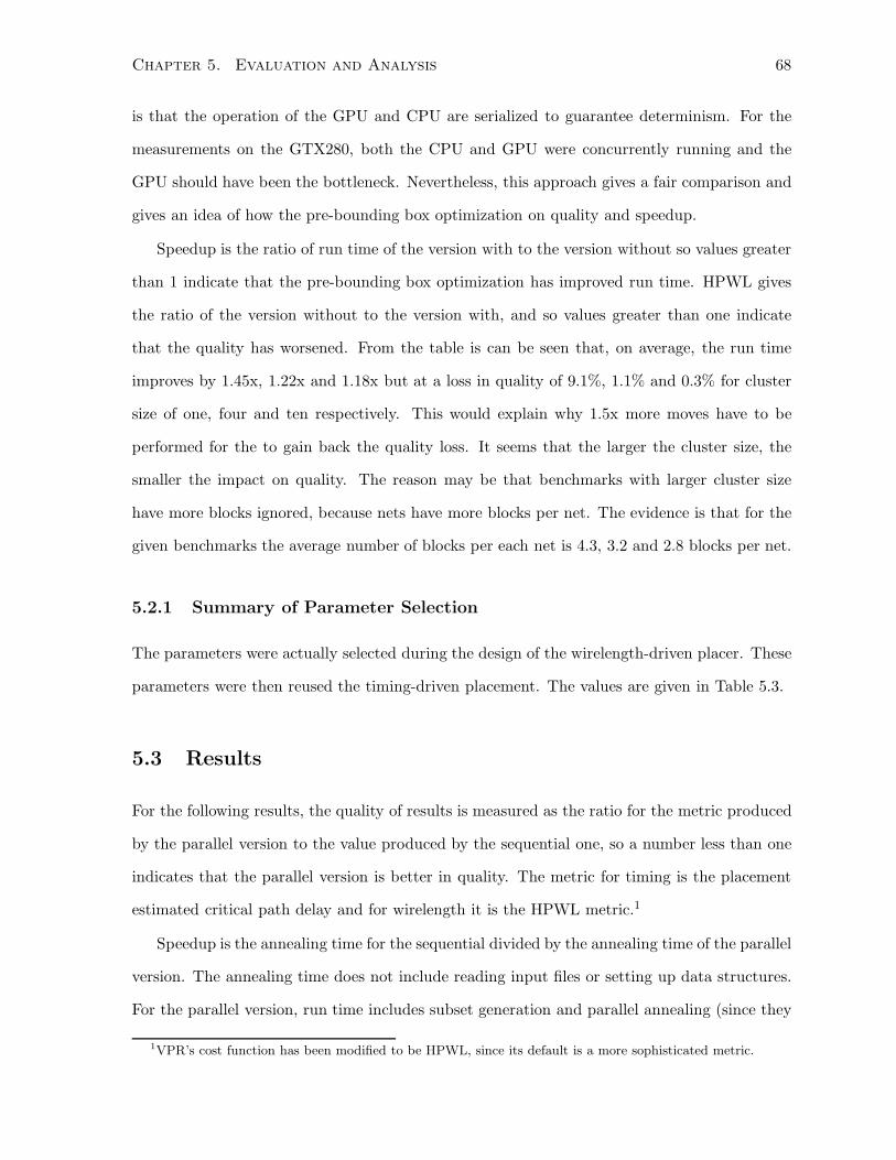
Chapter 5. Evaluation and Analysis 68
is that the operation of the GPU and CPU are serialized to guarantee determinism. For the
measurements on the GTX280, both the CPU and GPU were concurrently running and the
GPU should have been the bottleneck. Nevertheless, this approach gives a fair comparison and
gives an idea of how the pre-bounding box optimization on quality and speedup.
Speedup is the ratio of run time of the version with to the version without so values greater
than 1 indicate that the pre-bounding box optimization has improved run time. HPWL gives
the ratio of the version without to the version with, and so values greater than one indicate
that the quality has worsened. From the table is can be seen that, on average, the run time
improves by 1.45x, 1.22x and 1.18x but at a loss in quality of 9.1%, 1.1% and 0.3% for cluster
size of one, four and ten respectively. This would explain why 1.5x more moves have to be
performed for the to gain back the quality loss. It seems that the larger the cluster size, the
smaller the impact on quality. The reason may be that benchmarks with larger cluster size
have more blocks ignored, because nets have more blocks per net. The evidence is that for the
given benchmarks the average number of blocks per each net is 4.3, 3.2 and 2.8 blocks per net.
5.2.1 Summary of Parameter Selection
The parameters were actually selected during the design of the wirelength-driven placer. These
parameters were then reused the timing-driven placement. The values are given in Table 5.3.
5.3 Results
For the following results, the quality of results is measured as the ratio for the metric produced
by the parallel version to the value produced by the sequential one, so a number less than one
indicates that the parallel version is better in quality. The metric for timing is the placement
estimated critical path delay and for wirelength it is the HPWL metric.1
Speedup is the annealing time for the sequential divided by the annealing time of the parallel
version. The annealing time does not include reading input files or setting up data structures.
For the parallel version, run time includes subset generation and parallel annealing (since they
1VPR’s cost function has been modified to be HPWL, since its default is a more sophisticated metric.
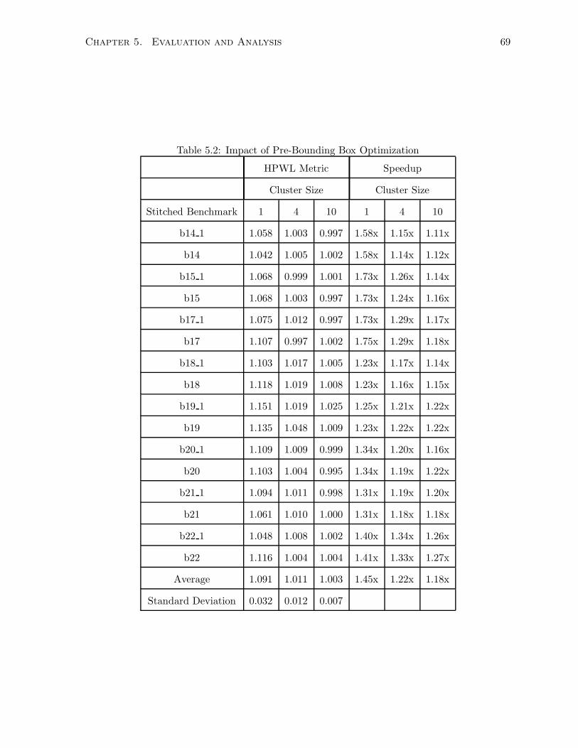
Chapter 5. Evaluation and Analysis 69
Table 5.2: Impact of Pre-Bounding Box Optimization
HPWL Metric Speedup
Cluster Size Cluster Size
Stitched Benchmark 1 4 10 1 4 10
b14 1 1.058 1.003 0.997 1.58x 1.15x 1.11x
b14 1.042 1.005 1.002 1.58x 1.14x 1.12x
b15 1 1.068 0.999 1.001 1.73x 1.26x 1.14x
b15 1.068 1.003 0.997 1.73x 1.24x 1.16x
b17 1 1.075 1.012 0.997 1.73x 1.29x 1.17x
b17 1.107 0.997 1.002 1.75x 1.29x 1.18x
b18 1 1.103 1.017 1.005 1.23x 1.17x 1.14x
b18 1.118 1.019 1.008 1.23x 1.16x 1.15x
b19 1 1.151 1.019 1.025 1.25x 1.21x 1.22x
b19 1.135 1.048 1.009 1.23x 1.22x 1.22x
b20 1 1.109 1.009 0.999 1.34x 1.20x 1.16x
b20 1.103 1.004 0.995 1.34x 1.19x 1.22x
b21 1 1.094 1.011 0.998 1.31x 1.19x 1.20x
b21 1.061 1.010 1.000 1.31x 1.18x 1.18x
b22 1 1.048 1.008 1.002 1.40x 1.34x 1.26x
b22 1.116 1.004 1.004 1.41x 1.33x 1.27x
Average 1.091 1.011 1.003 1.45x 1.22x 1.18x
Standard Deviation 0.032 0.012 0.007
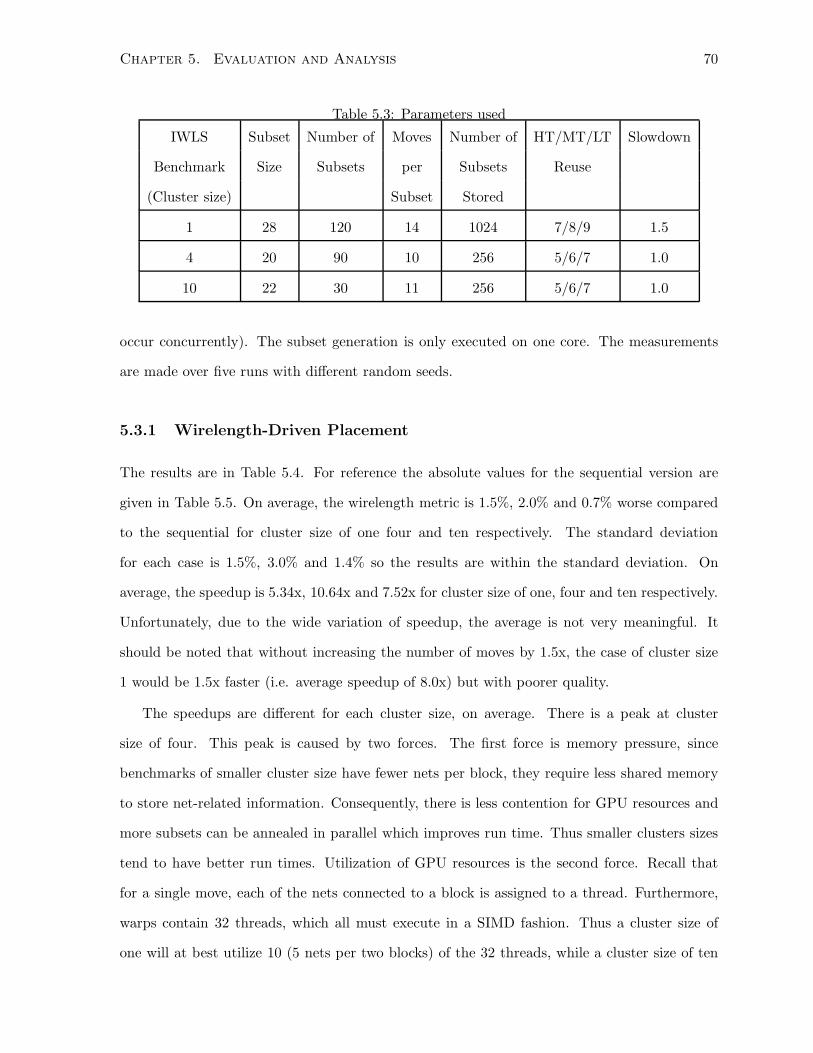
Chapter 5. Evaluation and Analysis 70
Table 5.3: Parameters used
IWLS Subset Number of Moves Number of HT/MT/LT Slowdown
Benchmark Size Subsets per Subsets Reuse
(Cluster size) Subset Stored
1 28 120 14 1024 7/8/9 1.5
4 20 90 10 256 5/6/7 1.0
10 22 30 11 256 5/6/7 1.0
occur concurrently). The subset generation is only executed on one core. The measurements
are made over five runs with different random seeds.
5.3.1 Wirelength-Driven Placement
The results are in Table 5.4. For reference the absolute values for the sequential version are
given in Table 5.5. On average, the wirelength metric is 1.5%, 2.0% and 0.7% worse compared
to the sequential for cluster size of one four and ten respectively. The standard deviation
for each case is 1.5%, 3.0% and 1.4% so the results are within the standard deviation. On
average, the speedup is 5.34x, 10.64x and 7.52x for cluster size of one, four and ten respectively.
Unfortunately, due to the wide variation of speedup, the average is not very meaningful. It
should be noted that without increasing the number of moves by 1.5x, the case of cluster size
1 would be 1.5x faster (i.e. average speedup of 8.0x) but with poorer quality.
The speedups are different for each cluster size, on average. There is a peak at cluster
size of four. This peak is caused by two forces. The first force is memory pressure, since
benchmarks of smaller cluster size have fewer nets per block, they require less shared memory
to store net-related information. Consequently, there is less contention for GPU resources and
more subsets can be annealed in parallel which improves run time. Thus smaller clusters sizes
tend to have better run times. Utilization of GPU resources is the second force. Recall that
for a single move, each of the nets connected to a block is assigned to a thread. Furthermore,
warps contain 32 threads, which all must execute in a SIMD fashion. Thus a cluster size of
one will at best utilize 10 (5 nets per two blocks) of the 32 threads, while a cluster size of ten
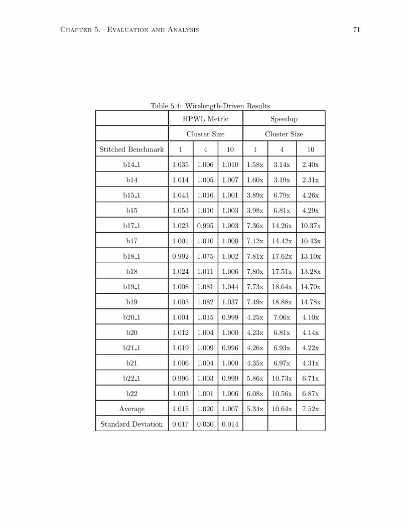
Chapter 5. Evaluation and Analysis 71
Table 5.4: Wirelength-Driven Results
HPWL Metric Speedup
Cluster Size Cluster Size
Stitched Benchmark 1 4 10 1 4 10
b14 1 1.035 1.006 1.010 1.58x 3.14x 2.40x
b14 1.014 1.005 1.007 1.60x 3.19x 2.31x
b15 1 1.043 1.016 1.001 3.89x 6.79x 4.26x
b15 1.053 1.010 1.003 3.98x 6.81x 4.29x
b17 1 1.023 0.995 1.003 7.36x 14.26x 10.37x
b17 1.001 1.010 1.000 7.12x 14.42x 10.43x
b18 1 0.992 1.075 1.002 7.81x 17.62x 13.10x
b18 1.024 1.011 1.006 7.80x 17.51x 13.28x
b19 1 1.008 1.081 1.044 7.73x 18.64x 14.70x
b19 1.005 1.082 1.037 7.49x 18.88x 14.78x
b20 1 1.004 1.015 0.999 4.25x 7.06x 4.10x
b20 1.012 1.004 1.000 4.23x 6.81x 4.14x
b21 1 1.019 1.009 0.996 4.26x 6.93x 4.22x
b21 1.006 1.004 1.000 4.35x 6.97x 4.31x
b22 1 0.996 1.003 0.999 5.86x 10.73x 6.71x
b22 1.003 1.001 1.006 6.08x 10.56x 6.87x
Average 1.015 1.020 1.007 5.34x 10.64x 7.52x
Standard Deviation 0.017 0.030 0.014
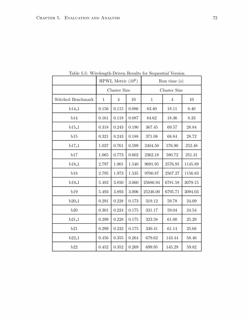
Chapter 5. Evaluation and Analysis 72
Table 5.5: Wirelength-Driven Results for Sequential Version
HPWL Metric (106) Run time (s)
Cluster Size Cluster Size
Stitched Benchmark 1 4 10 1 4 10
b14 1 0.156 0.115 0.086 83.40 18.11 8.40
b14 0.161 0.118 0.087 84.62 18.36 8.33
b15 1 0.318 0.243 0.190 367.45 69.57 28.84
b15 0.321 0.243 0.188 371.08 68.84 28.72
b17 1 1.037 0.761 0.599 2404.50 576.90 252.48
b17 1.065 0.773 0.602 2362.18 580.72 251.31
b18 1 2.797 1.901 1.540 9691.95 2576.95 1145.89
b18 2.795 1.973 1.535 9700.87 2567.27 1156.83
b19 1 5.482 3.850 3.060 25686.94 6781.58 3079.15
b19 5.493 3.893 3.006 25246.00 6795.71 3094.03
b20 1 0.291 0.228 0.173 319.12 59.78 24.09
b20 0.301 0.224 0.175 321.17 59.04 24.54
b21 1 0.299 0.228 0.175 323.58 61.00 25.29
b21 0.299 0.232 0.175 330.41 61.14 25.68
b22 1 0.456 0.355 0.264 679.62 143.44 58.46
b22 0.452 0.352 0.269 699.95 145.29 59.82
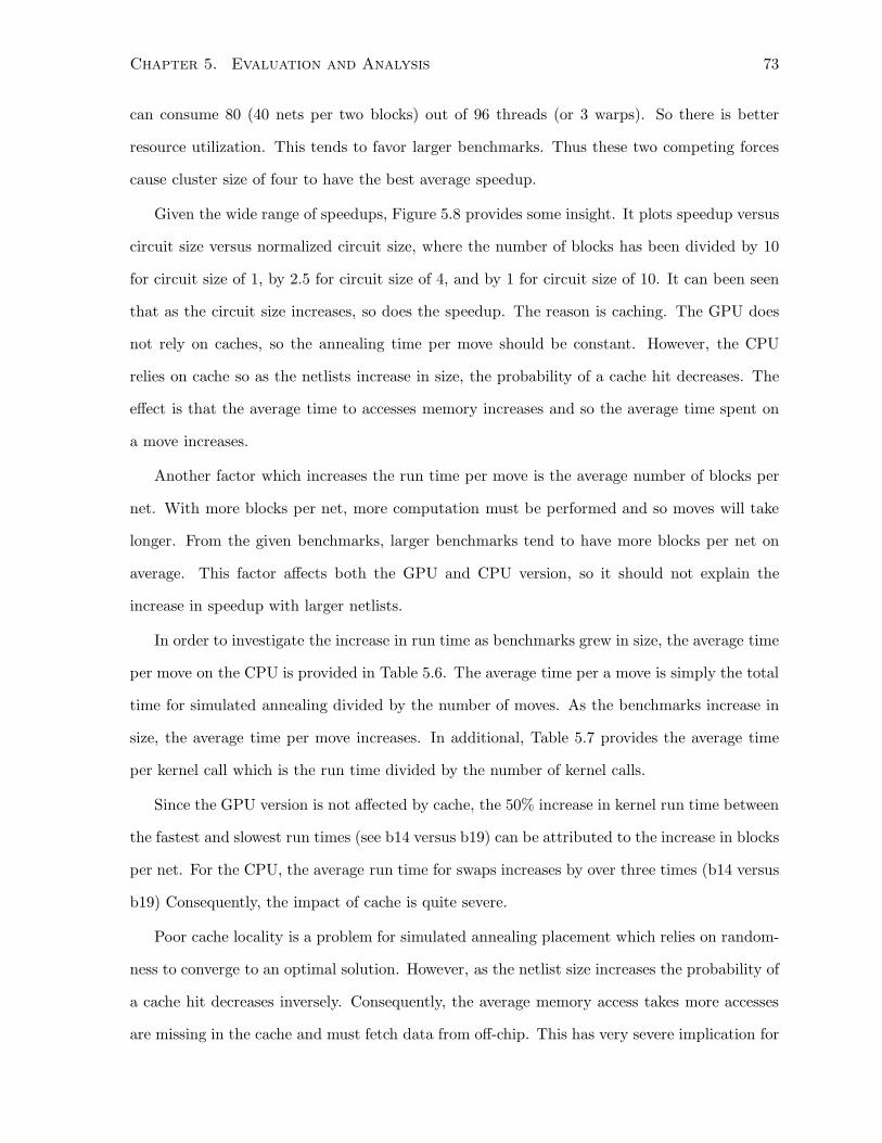
Chapter 5. Evaluation and Analysis 73
can consume 80 (40 nets per two blocks) out of 96 threads (or 3 warps). So there is better
resource utilization. This tends to favor larger benchmarks. Thus these two competing forces
cause cluster size of four to have the best average speedup.
Given the wide range of speedups, Figure 5.8 provides some insight. It plots speedup versus
circuit size versus normalized circuit size, where the number of blocks has been divided by 10
for circuit size of 1, by 2.5 for circuit size of 4, and by 1 for circuit size of 10. It can been seen
that as the circuit size increases, so does the speedup. The reason is caching. The GPU does
not rely on caches, so the annealing time per move should be constant. However, the CPU
relies on cache so as the netlists increase in size, the probability of a cache hit decreases. The
effect is that the average time to accesses memory increases and so the average time spent on
a move increases.
Another factor which increases the run time per move is the average number of blocks per
net. With more blocks per net, more computation must be performed and so moves will take
longer. From the given benchmarks, larger benchmarks tend to have more blocks per net on
average. This factor affects both the GPU and CPU version, so it should not explain the
increase in speedup with larger netlists.
In order to investigate the increase in run time as benchmarks grew in size, the average time
per move on the CPU is provided in Table 5.6. The average time per a move is simply the total
time for simulated annealing divided by the number of moves. As the benchmarks increase in
size, the average time per move increases. In additional, Table 5.7 provides the average time
per kernel call which is the run time divided by the number of kernel calls.
Since the GPU version is not affected by cache, the 50% increase in kernel run time between
the fastest and slowest run times (see b14 versus b19) can be attributed to the increase in blocks
per net. For the CPU, the average run time for swaps increases by over three times (b14 versus
b19) Consequently, the impact of cache is quite severe.
Poor cache locality is a problem for simulated annealing placement which relies on random-
ness to converge to an optimal solution. However, as the netlist size increases the probability of
a cache hit decreases inversely. Consequently, the average memory access takes more accesses
are missing in the cache and must fetch data from off-chip. This has very severe implication for
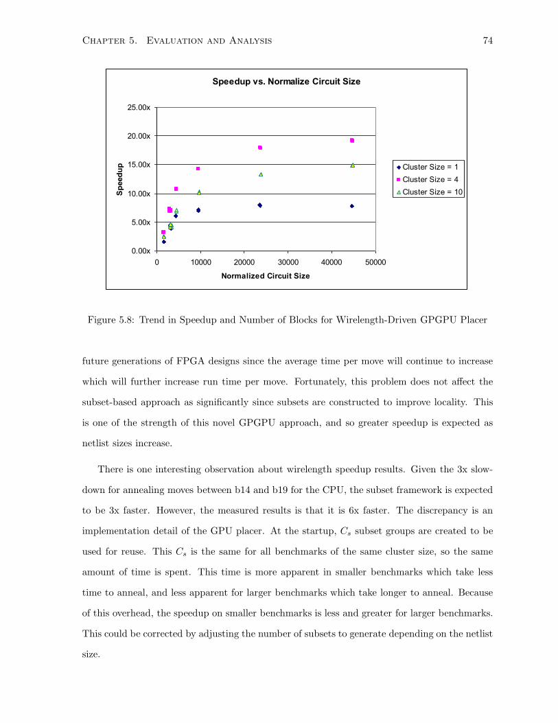
Chapter 5. Evaluation and Analysis 74
Speedup vs. Normalize Circuit Size
0.00x
5.00x
10.00x
15.00x
20.00x
25.00x
0 10000 20000 30000 40000 50000
Normalized Circuit Size
Sp
eed
up Cluster Size = 1
Cluster Size = 4
Cluster Size = 10
Figure 5.8: Trend in Speedup and Number of Blocks for Wirelength-Driven GPGPU Placer
future generations of FPGA designs since the average time per move will continue to increase
which will further increase run time per move. Fortunately, this problem does not affect the
subset-based approach as significantly since subsets are constructed to improve locality. This
is one of the strength of this novel GPGPU approach, and so greater speedup is expected as
netlist sizes increase.
There is one interesting observation about wirelength speedup results. Given the 3x slow-
down for annealing moves between b14 and b19 for the CPU, the subset framework is expected
to be 3x faster. However, the measured results is that it is 6x faster. The discrepancy is an
implementation detail of the GPU placer. At the startup, Cs subset groups are created to be
used for reuse. This Cs is the same for all benchmarks of the same cluster size, so the same
amount of time is spent. This time is more apparent in smaller benchmarks which take less
time to anneal, and less apparent for larger benchmarks which take longer to anneal. Because
of this overhead, the speedup on smaller benchmarks is less and greater for larger benchmarks.
This could be corrected by adjusting the number of subsets to generate depending on the netlist
size.
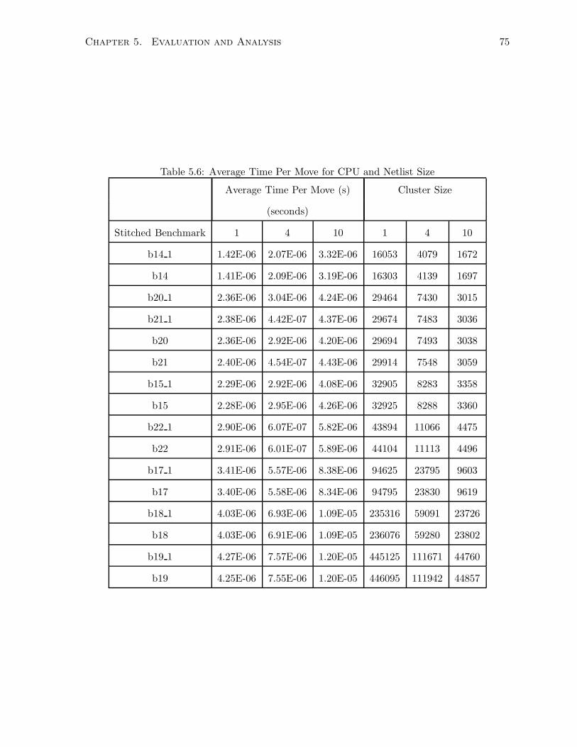
Chapter 5. Evaluation and Analysis 75
Table 5.6: Average Time Per Move for CPU and Netlist Size
Average Time Per Move (s) Cluster Size
(seconds)
Stitched Benchmark 1 4 10 1 4 10
b14 1 1.42E-06 2.07E-06 3.32E-06 16053 4079 1672
b14 1.41E-06 2.09E-06 3.19E-06 16303 4139 1697
b20 1 2.36E-06 3.04E-06 4.24E-06 29464 7430 3015
b21 1 2.38E-06 4.42E-07 4.37E-06 29674 7483 3036
b20 2.36E-06 2.92E-06 4.20E-06 29694 7493 3038
b21 2.40E-06 4.54E-07 4.43E-06 29914 7548 3059
b15 1 2.29E-06 2.92E-06 4.08E-06 32905 8283 3358
b15 2.28E-06 2.95E-06 4.26E-06 32925 8288 3360
b22 1 2.90E-06 6.07E-07 5.82E-06 43894 11066 4475
b22 2.91E-06 6.01E-07 5.89E-06 44104 11113 4496
b17 1 3.41E-06 5.57E-06 8.38E-06 94625 23795 9603
b17 3.40E-06 5.58E-06 8.34E-06 94795 23830 9619
b18 1 4.03E-06 6.93E-06 1.09E-05 235316 59091 23726
b18 4.03E-06 6.91E-06 1.09E-05 236076 59280 23802
b19 1 4.27E-06 7.57E-06 1.20E-05 445125 111671 44760
b19 4.25E-06 7.55E-06 1.20E-05 446095 111942 44857
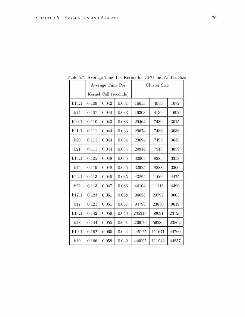
Chapter 5. Evaluation and Analysis 76
Table 5.7: Average Time Per Kernel for GPU and Netlist Size
Average Time Per Cluster Size
Kernel Call (seconds)
b14 1 0.109 0.042 0.031 16053 4079 1672
b14 0.107 0.044 0.033 16303 4139 1697
b20 1 0.110 0.043 0.033 29464 7430 3015
b21 1 0.111 0.044 0.033 29674 7483 3036
b20 0.111 0.044 0.034 29694 7493 3038
b21 0.111 0.044 0.034 29914 7548 3059
b15 1 0.125 0.048 0.035 32905 8283 3358
b15 0.119 0.048 0.035 32925 8288 3360
b22 1 0.113 0.045 0.035 43894 11066 4475
b22 0.113 0.047 0.036 44104 11113 4496
b17 1 0.123 0.051 0.038 94625 23795 9603
b17 0.121 0.051 0.037 94795 23830 9619
b18 1 0.142 0.059 0.043 235316 59091 23726
b18 0.144 0.055 0.041 236076 59280 23802
b19 1 0.162 0.060 0.044 445125 111671 44760
b19 0.166 0.059 0.042 446095 111942 44857
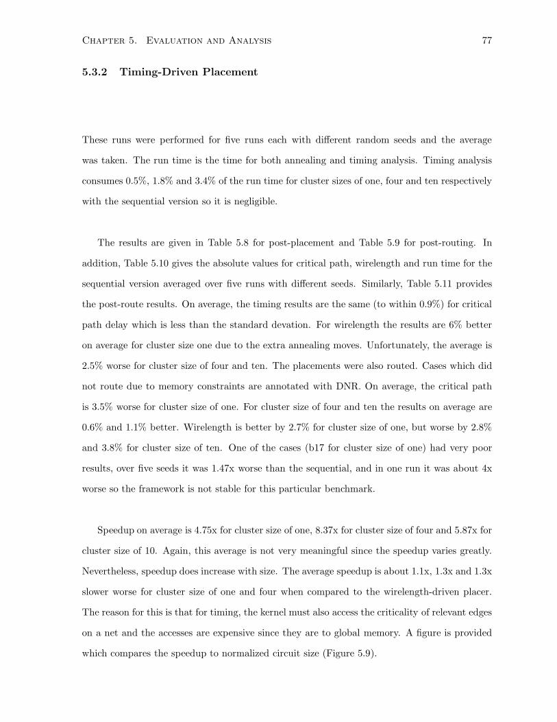
Chapter 5. Evaluation and Analysis 77
5.3.2 Timing-Driven Placement
These runs were performed for five runs each with different random seeds and the average
was taken. The run time is the time for both annealing and timing analysis. Timing analysis
consumes 0.5%, 1.8% and 3.4% of the run time for cluster sizes of one, four and ten respectively
with the sequential version so it is negligible.
The results are given in Table 5.8 for post-placement and Table 5.9 for post-routing. In
addition, Table 5.10 gives the absolute values for critical path, wirelength and run time for the
sequential version averaged over five runs with different seeds. Similarly, Table 5.11 provides
the post-route results. On average, the timing results are the same (to within 0.9%) for critical
path delay which is less than the standard devation. For wirelength the results are 6% better
on average for cluster size one due to the extra annealing moves. Unfortunately, the average is
2.5% worse for cluster size of four and ten. The placements were also routed. Cases which did
not route due to memory constraints are annotated with DNR. On average, the critical path
is 3.5% worse for cluster size of one. For cluster size of four and ten the results on average are
0.6% and 1.1% better. Wirelength is better by 2.7% for cluster size of one, but worse by 2.8%
and 3.8% for cluster size of ten. One of the cases (b17 for cluster size of one) had very poor
results, over five seeds it was 1.47x worse than the sequential, and in one run it was about 4x
worse so the framework is not stable for this particular benchmark.
Speedup on average is 4.75x for cluster size of one, 8.37x for cluster size of four and 5.87x for
cluster size of 10. Again, this average is not very meaningful since the speedup varies greatly.
Nevertheless, speedup does increase with size. The average speedup is about 1.1x, 1.3x and 1.3x
slower worse for cluster size of one and four when compared to the wirelength-driven placer.
The reason for this is that for timing, the kernel must also access the criticality of relevant edges
on a net and the accesses are expensive since they are to global memory. A figure is provided
which compares the speedup to normalized circuit size (Figure 5.9).
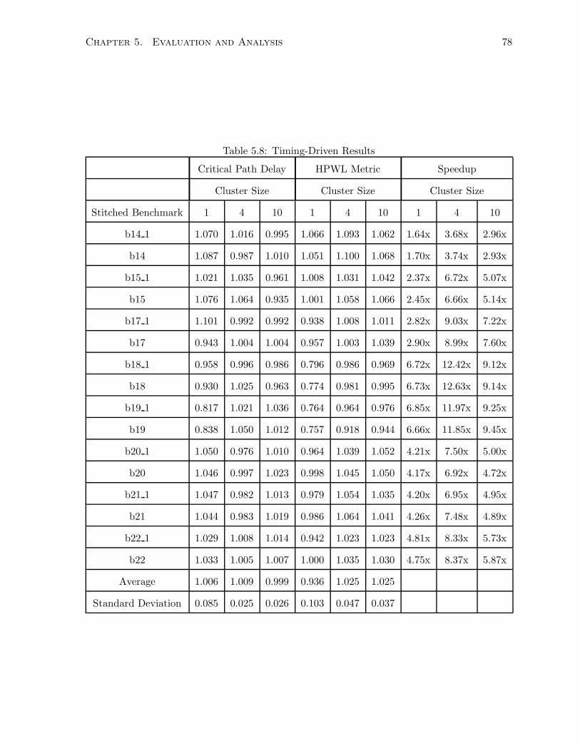
Chapter 5. Evaluation and Analysis 78
Table 5.8: Timing-Driven Results
Critical Path Delay HPWL Metric Speedup
Cluster Size Cluster Size Cluster Size
Stitched Benchmark 1 4 10 1 4 10 1 4 10
b14 1 1.070 1.016 0.995 1.066 1.093 1.062 1.64x 3.68x 2.96x
b14 1.087 0.987 1.010 1.051 1.100 1.068 1.70x 3.74x 2.93x
b15 1 1.021 1.035 0.961 1.008 1.031 1.042 2.37x 6.72x 5.07x
b15 1.076 1.064 0.935 1.001 1.058 1.066 2.45x 6.66x 5.14x
b17 1 1.101 0.992 0.992 0.938 1.008 1.011 2.82x 9.03x 7.22x
b17 0.943 1.004 1.004 0.957 1.003 1.039 2.90x 8.99x 7.60x
b18 1 0.958 0.996 0.986 0.796 0.986 0.969 6.72x 12.42x 9.12x
b18 0.930 1.025 0.963 0.774 0.981 0.995 6.73x 12.63x 9.14x
b19 1 0.817 1.021 1.036 0.764 0.964 0.976 6.85x 11.97x 9.25x
b19 0.838 1.050 1.012 0.757 0.918 0.944 6.66x 11.85x 9.45x
b20 1 1.050 0.976 1.010 0.964 1.039 1.052 4.21x 7.50x 5.00x
b20 1.046 0.997 1.023 0.998 1.045 1.050 4.17x 6.92x 4.72x
b21 1 1.047 0.982 1.013 0.979 1.054 1.035 4.20x 6.95x 4.95x
b21 1.044 0.983 1.019 0.986 1.064 1.041 4.26x 7.48x 4.89x
b22 1 1.029 1.008 1.014 0.942 1.023 1.023 4.81x 8.33x 5.73x
b22 1.033 1.005 1.007 1.000 1.035 1.030 4.75x 8.37x 5.87x
Average 1.006 1.009 0.999 0.936 1.025 1.025
Standard Deviation 0.085 0.025 0.026 0.103 0.047 0.037
Chapter 5. Evaluation and Analysis 79
Table 5.9: Post-Routing Results
Critical Path Delay Wirelength
1 4 10 1 4 10
b14 1 1.002 0.993 0.989 1.007 1.086 1.057
b14 1.018 0.983 0.998 0.983 1.083 1.072
b15 1 0.923 1.020 0.951 0.951 1.029 1.045
b15 0.941 1.032 0.928 0.958 1.053 1.067
b17 1 1.064 0.959 0.985 0.914 1.009 1.016
b17 1.476 0.981 0.981 0.928 1.009 1.047
b18 1 DNR 0.986 0.982 DNR 0.992 0.983
b18 DNR 1.017 0.963 DNR 0.987 1.010
b19 1 DNR 1.002 1.021 DNR 0.975 0.983
b19 DNR 1.054 DNR DNR 0.933 DNR
b20 1 1.001 0.964 1.003 0.967 1.048 1.061
b20 1.005 0.980 1.011 0.977 1.047 1.055
b21 1 0.988 0.974 1.001 0.975 1.055 1.044
b21 1.006 0.977 1.012 0.970 1.063 1.046
b22 1 1.007 0.992 1.015 0.949 1.033 1.035
b22 0.985 0.989 0.997 0.981 1.039 1.042
Average 1.035 0.994 0.989 0.963 1.028 1.038
Standard Deviation 0.143 0.025 0.026 0.025 0.041 0.028
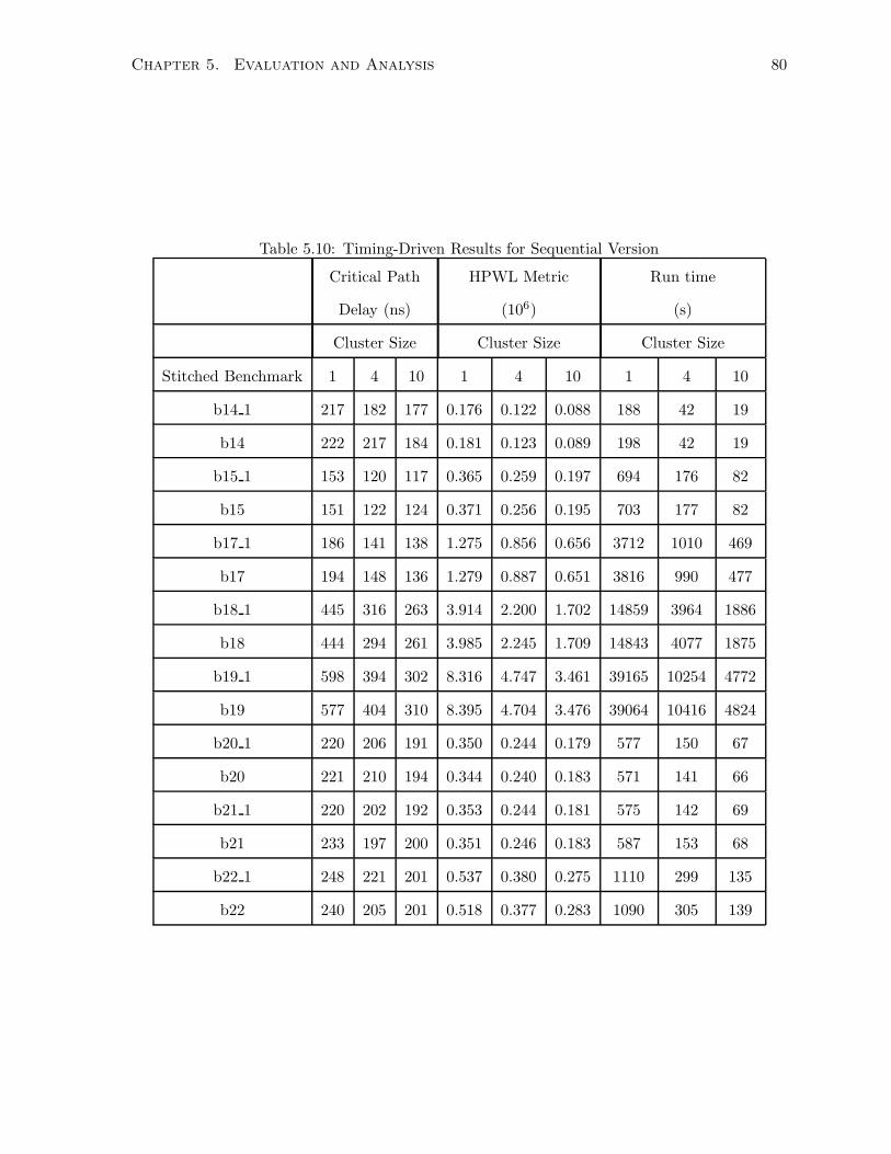
Chapter 5. Evaluation and Analysis 80
Table 5.10: Timing-Driven Results for Sequential Version
Critical Path HPWL Metric Run time
Delay (ns) (106) (s)
Cluster Size Cluster Size Cluster Size
Stitched Benchmark 1 4 10 1 4 10 1 4 10
b14 1 217 182 177 0.176 0.122 0.088 188 42 19
b14 222 217 184 0.181 0.123 0.089 198 42 19
b15 1 153 120 117 0.365 0.259 0.197 694 176 82
b15 151 122 124 0.371 0.256 0.195 703 177 82
b17 1 186 141 138 1.275 0.856 0.656 3712 1010 469
b17 194 148 136 1.279 0.887 0.651 3816 990 477
b18 1 445 316 263 3.914 2.200 1.702 14859 3964 1886
b18 444 294 261 3.985 2.245 1.709 14843 4077 1875
b19 1 598 394 302 8.316 4.747 3.461 39165 10254 4772
b19 577 404 310 8.395 4.704 3.476 39064 10416 4824
b20 1 220 206 191 0.350 0.244 0.179 577 150 67
b20 221 210 194 0.344 0.240 0.183 571 141 66
b21 1 220 202 192 0.353 0.244 0.181 575 142 69
b21 233 197 200 0.351 0.246 0.183 587 153 68
b22 1 248 221 201 0.537 0.380 0.275 1110 299 135
b22 240 205 201 0.518 0.377 0.283 1090 305 139
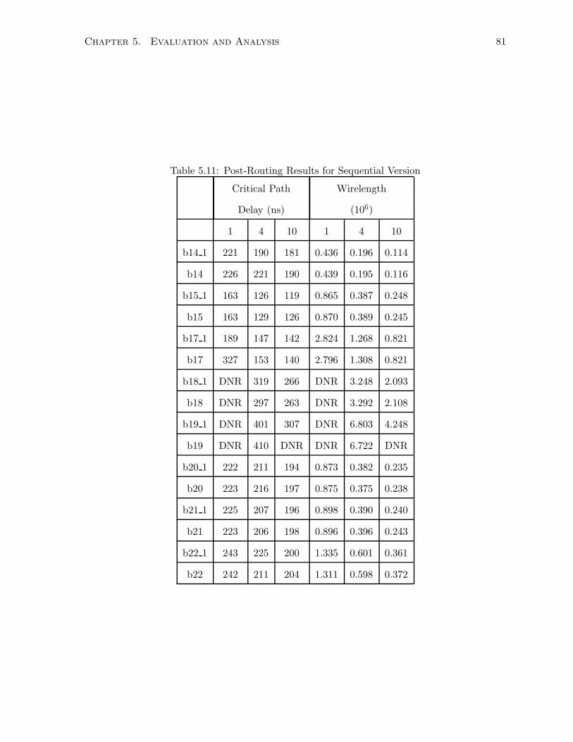
Chapter 5. Evaluation and Analysis 81
Table 5.11: Post-Routing Results for Sequential Version
Critical Path Wirelength
Delay (ns) (106)
1 4 10 1 4 10
b14 1 221 190 181 0.436 0.196 0.114
b14 226 221 190 0.439 0.195 0.116
b15 1 163 126 119 0.865 0.387 0.248
b15 163 129 126 0.870 0.389 0.245
b17 1 189 147 142 2.824 1.268 0.821
b17 327 153 140 2.796 1.308 0.821
b18 1 DNR 319 266 DNR 3.248 2.093
b18 DNR 297 263 DNR 3.292 2.108
b19 1 DNR 401 307 DNR 6.803 4.248
b19 DNR 410 DNR DNR 6.722 DNR
b20 1 222 211 194 0.873 0.382 0.235
b20 223 216 197 0.875 0.375 0.238
b21 1 225 207 196 0.898 0.390 0.240
b21 223 206 198 0.896 0.396 0.243
b22 1 243 225 200 1.335 0.601 0.361
b22 242 211 204 1.311 0.598 0.372
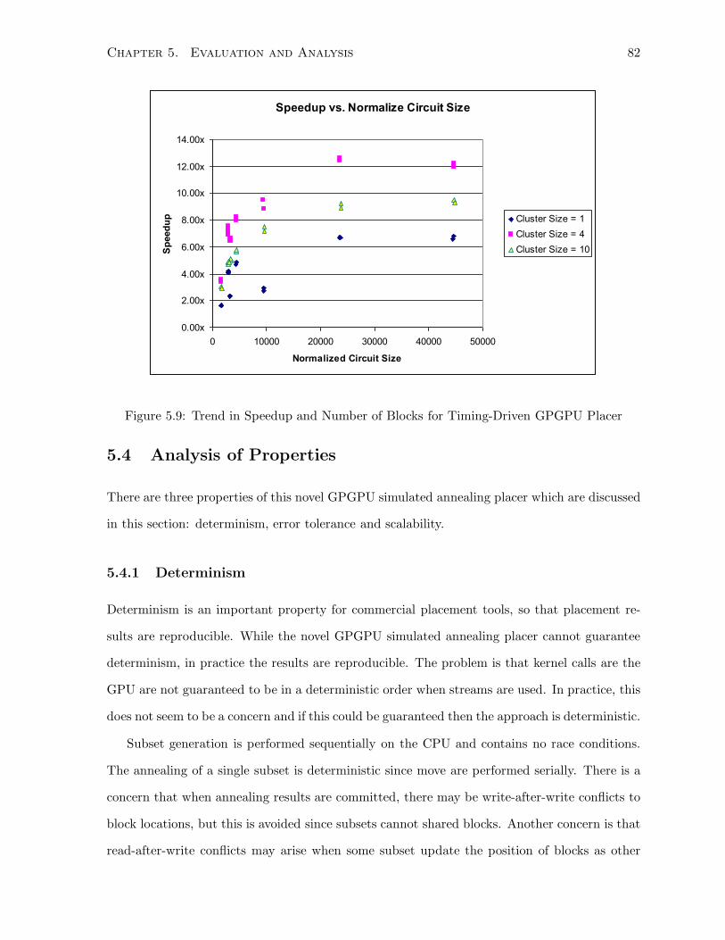
Chapter 5. Evaluation and Analysis 82
Speedup vs. Normalize Circuit Size
0.00x
2.00x
4.00x
6.00x
8.00x
10.00x
12.00x
14.00x
0 10000 20000 30000 40000 50000
Normalized Circuit Size
Sp
eed
up Cluster Size = 1
Cluster Size = 4
Cluster Size = 10
Figure 5.9: Trend in Speedup and Number of Blocks for Timing-Driven GPGPU Placer
5.4 Analysis of Properties
There are three properties of this novel GPGPU simulated annealing placer which are discussed
in this section: determinism, error tolerance and scalability.
5.4.1 Determinism
Determinism is an important property for commercial placement tools, so that placement re-
sults are reproducible. While the novel GPGPU simulated annealing placer cannot guarantee
determinism, in practice the results are reproducible. The problem is that kernel calls are the
GPU are not guaranteed to be in a deterministic order when streams are used. In practice, this
does not seem to be a concern and if this could be guaranteed then the approach is deterministic.
Subset generation is performed sequentially on the CPU and contains no race conditions.
The annealing of a single subset is deterministic since move are performed serially. There is a
concern that when annealing results are committed, there may be write-after-write conflicts to
block locations, but this is avoided since subsets cannot shared blocks. Another concern is that
read-after-write conflicts may arise when some subset update the position of blocks as other
Chapter 5. Evaluation and Analysis 83
subsets are reading the same position to compute the pre-bounding box. This is prevented by
using two kernel calls. The first reads all the placement data, performs a set of moves, and
writes the new results to a temporary buffer (which is only writeable by a single subset). The
second uses the temporary buffer to write the block positions. For the previous generation of
GPU (GTX280), we used the asynchronous API to improve concurrency via streams, and this
may give rise to non-deterministic ordering for kernel calls. Table 5.12 gives the speedup and
quality of results, if streams are not used.2 For these results, only one seed was used, because
the goal is to assess the impact on run time. The variance for run time is less than 2%, but the
comparison is between run times which are about two times larger, so the noise is negligible.
From the table is can be seen that the allowing for concurrent execution is on average 3.55x,
4.96x and 3.88x faster for cluster size of one, four and ten (compared to 5.34x, 10.64x and 7.72x
with concurrent execution).
Empirically, the approach is reproducible. The algorithm was run three times for all bench-
marks and all three trials they produced exactly the same placement results. May be due to
one of two reasons. Firstly, the driver may be deterministic, but the NVIDIA simply does
not guarantee determinism. The motivation for streams is to improve runtime by aggressively
executing memory transfers and kernel calls as soon as they are available. It may be that the
current driver is not as sophisticated and simply executes in a first in first out order. Therefore,
the results are reproducible, but it is not possible to guarantee determinism in the strictest.
5.4.2 Error Tolerance
Another property of this novel placer is its tolerance for errors, since this parallelization frame-
work introduces errors which are not present in the sequential version. By error, it is meant
that the computation of the cost metric may be different on the parallel version when compared
the sequential version. In this framework, the difference arises because each SMP assumes that
all other SMPs are inactive when it evaluates the cost metric. However, the other SMPs are
active, so there is a difference between the metric as computed on the SMP versus if the SMP
2To be precise, the implementation used exactly one stream, which is equivalent to not using streams sinceCPU, GPU and memory operations are serialized.
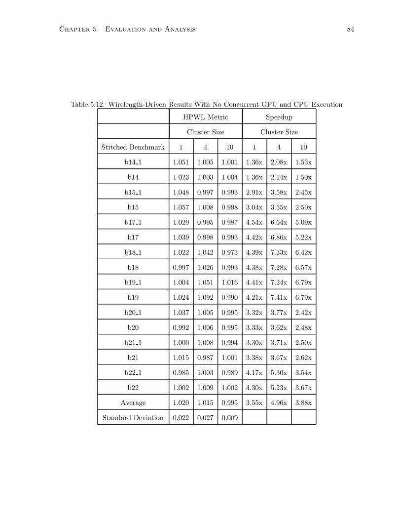
Chapter 5. Evaluation and Analysis 84
Table 5.12: Wirelength-Driven Results With No Concurrent GPU and CPU Execution
HPWL Metric Speedup
Cluster Size Cluster Size
Stitched Benchmark 1 4 10 1 4 10
b14 1 1.051 1.005 1.001 1.36x 2.08x 1.53x
b14 1.023 1.003 1.004 1.36x 2.14x 1.50x
b15 1 1.048 0.997 0.993 2.91x 3.58x 2.45x
b15 1.057 1.008 0.998 3.04x 3.55x 2.50x
b17 1 1.029 0.995 0.987 4.54x 6.64x 5.09x
b17 1.039 0.998 0.993 4.42x 6.86x 5.22x
b18 1 1.022 1.042 0.973 4.39x 7.33x 6.42x
b18 0.997 1.026 0.993 4.38x 7.28x 6.57x
b19 1 1.004 1.051 1.016 4.41x 7.24x 6.79x
b19 1.024 1.092 0.990 4.21x 7.41x 6.79x
b20 1 1.037 1.005 0.995 3.32x 3.77x 2.42x
b20 0.992 1.006 0.995 3.33x 3.62x 2.48x
b21 1 1.000 1.008 0.994 3.30x 3.71x 2.50x
b21 1.015 0.987 1.001 3.38x 3.67x 2.62x
b22 1 0.985 1.003 0.989 4.17x 5.30x 3.54x
b22 1.002 1.009 1.002 4.30x 5.23x 3.67x
Average 1.020 1.015 0.995 3.55x 4.96x 3.88x
Standard Deviation 0.022 0.027 0.009
Chapter 5. Evaluation and Analysis 85
assumed the other processors were active.
These errors do no accumulate because of the behavior of the kernel. When the kernel is
executed on an SMP it reads the position of all blocks in the subset and all blocks connected to
it3. Consequently, the first move will use data that should not be very stale, but the error will
accumulate, until the kernel finishes. At this point all the new block positions are committed
so that the next kernel call will start with fresh data. Consequently, the error is temporary
because the end of each kernel acts as a synchronization point.
Despite these errors, the GPGPU simulated annealer still converges to the good solutions
solution in comparison with the sequential version. These findings are in agreement with pre-
vious work. Durand reports that previous works which have temporary error are capable of
converging to “good” solutions [17]. Rose et al. also found that if not more than ten moves are
performed between updating local copies of placement information, then there is no problem
with convergence [31]. Our approach uses between 11-14 moves per subset. Similarly, work by
Sun and Sechen implemented a system with temporary error and were able to obtain results
with almost no loss in quality compared to a sequential version on average [34]. Thus the
findings in this thesis are in agreement with previous work.
5.4.3 Scalability
The concern with scalability is that if the number of processors doubles the speedup will not
double. To investigate the scalability of the subset-based framework, the same scheme is ex-
ecuted on one of the next generation GPU’s from NVIDIA, the GTX480. This GPU has 480
SPs, which are organized into 16 SMPs with each having 32 SPs. The shared memory per
SMP is also increased to 48kB. Table 5.13 compares the specifications of each processor. An
interesting design decision is that the number of SPs has quadrupled per SMP. The increase
in SPs is used to increase performance. With the GTX280, 8 SPs are used to execute a single
warp of 32 threads, by repeating the same instruction over four cycles. For the GTX480, 16
SPs are used to execute the 32 threads over two cycles. So there is an effective speedup of 2x
3Because of the pre-bounding box information, the SMP will actually not read all the information at most P
blocks, where P is the pre-bounding optimization parameter. See Subsection 5.2.
Chapter 5. Evaluation and Analysis 86
for execution of instructions. There are 32 SPs within an SMP, so two warps can concurrently
execute.
There are other relevant changes are with the increase in shared memory and changes to
kernel execution on the GPU. In addition to the increase in SPs, shared memory per SMP has
tripled. Thus when implementing the subset-based framework on the GTX480, three times the
number of subsets are used. Table 5.14 lists all the parameters used, and they are the same as
the GTX280 except that the number of subsets have tripled. Also, the slowdown is set to either
1 or 1.5 to explore the impact of increasing the number of moves on quality and run time.
For kernel execution, the GTX480 allows kernel calls from different streams to be executed
concurrently on the GPU. In the GTX280, only one kernel could be executed at a time. While
the hope is that this would increase performance, this unfortunately makes the framework non-
deterministic and the results are not reproducible. To resolve this problem, only one stream is
used, so the queue length is one. This is equivalent to not using streams at all and prevents
the CPU and GPU from executing concurrently. The effect is that now kernel calls occur in a
deterministic order so the approach is deterministic. To better appreciate the run time impact
of preventing concurrent execution, Table 5.12 provides results which compare the run time and
quality of results for wirelength on the GTX280. When the GPU and CPU are not concurrent,
the speedups are 3.55x, 4.96x and 3.88x for cluster size of one, four and ten respectively, and
these are 1.5x, 2.1x and 1.9x slower than if concurrency is allowed.
Because concurrent kernel execution must be prevented on the GTX480, the implementation
is expected to be about 2x slower. So despite having twice as many SPs, the expected overall
speedup is expected to be one. Fortunately, for another architectural change, it will be seen that
the actually speedup for the timing metric will not be so poor. The change is that accesses to
global memory are now cached. This means that memory latency should be reduced, and this
helps the timing-driven implementation which makes accesses to global memory in a localized
manner.
Another change to the parallelization scheme is that the value of Cs is selected to be propor-
tional to the netlist size. This Cs is the number of subset groups stored, and roughly speaking,
that is the number of subsets which have to be generated when annealing starts. As observed
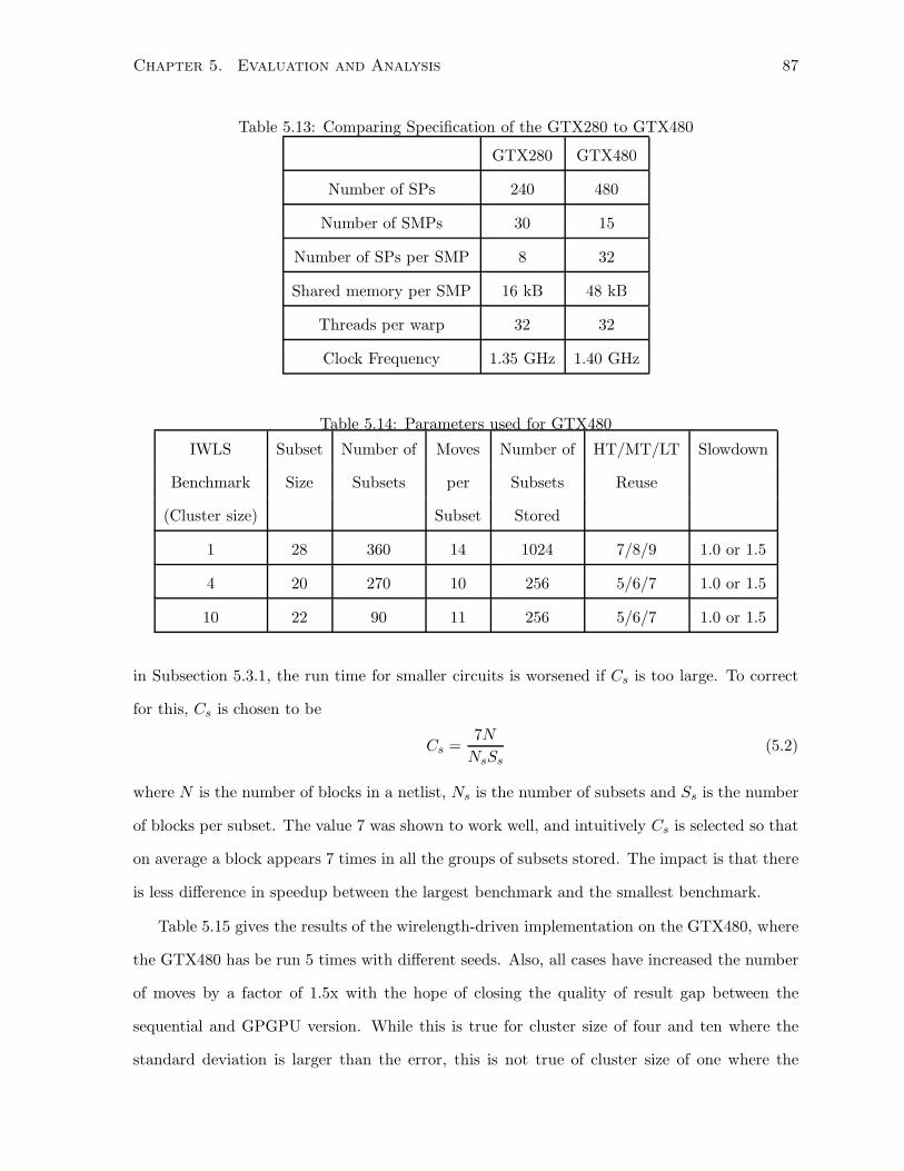
Chapter 5. Evaluation and Analysis 87
Table 5.13: Comparing Specification of the GTX280 to GTX480
GTX280 GTX480
Number of SPs 240 480
Number of SMPs 30 15
Number of SPs per SMP 8 32
Shared memory per SMP 16 kB 48 kB
Threads per warp 32 32
Clock Frequency 1.35 GHz 1.40 GHz
Table 5.14: Parameters used for GTX480
IWLS Subset Number of Moves Number of HT/MT/LT Slowdown
Benchmark Size Subsets per Subsets Reuse
(Cluster size) Subset Stored
1 28 360 14 1024 7/8/9 1.0 or 1.5
4 20 270 10 256 5/6/7 1.0 or 1.5
10 22 90 11 256 5/6/7 1.0 or 1.5
in Subsection 5.3.1, the run time for smaller circuits is worsened if Cs is too large. To correct
for this, Cs is chosen to be
Cs =7N
NsSs(5.2)
where N is the number of blocks in a netlist, Ns is the number of subsets and Ss is the number
of blocks per subset. The value 7 was shown to work well, and intuitively Cs is selected so that
on average a block appears 7 times in all the groups of subsets stored. The impact is that there
is less difference in speedup between the largest benchmark and the smallest benchmark.
Table 5.15 gives the results of the wirelength-driven implementation on the GTX480, where
the GTX480 has be run 5 times with different seeds. Also, all cases have increased the number
of moves by a factor of 1.5x with the hope of closing the quality of result gap between the
sequential and GPGPU version. While this is true for cluster size of four and ten where the
standard deviation is larger than the error, this is not true of cluster size of one where the
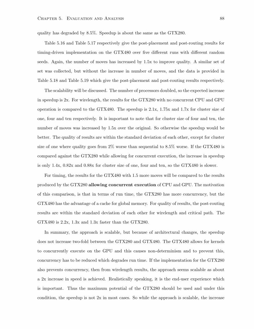
Chapter 5. Evaluation and Analysis 88
quality has degraded by 8.5%. Speedup is about the same as the GTX280.
Table 5.16 and Table 5.17 respectively give the post-placement and post-routing results for
timing-driven implementation on the GTX480 over five different runs with different random
seeds. Again, the number of moves has increased by 1.5x to improve quality. A similar set of
set was collected, but without the increase in number of moves, and the data is provided in
Table 5.18 and Table 5.19 which give the post-placement and post-routing results respectively.
The scalability will be discussed. The number of processors doubled, so the expected increase
in speedup is 2x. For wirelength, the results for the GTX280 with no concurrent CPU and GPU
operation is compared to the GTX480. The speedup is 2.1x, 1.75x and 1.7x for cluster size of
one, four and ten respectively. It is important to note that for cluster size of four and ten, the
number of moves was increased by 1.5x over the original. So otherwise the speedup would be
better. The quality of results are within the standard deviation of each other, except for cluster
size of one where quality goes from 2% worse than sequential to 8.5% worse. If the GTX480 is
compared against the GTX280 while allowing for concurrent execution, the increase in speedup
is only 1.4x, 0.82x and 0.88x for cluster size of one, four and ten, so the GTX480 is slower.
For timing, the results for the GTX480 with 1.5 more moves will be compared to the results
produced by the GTX280 allowing concurrent execution of CPU and GPU. The motivation
of this comparison, is that in terms of run time, the GTX280 has more concurrency, but the
GTX480 has the advantage of a cache for global memory. For quality of results, the post-routing
results are within the standard deviation of each other for wirelength and critical path. The
GTX480 is 2.2x, 1.3x and 1.3x faster than the GTX280.
In summary, the approach is scalable, but because of architectural changes, the speedup
does not increase two-fold between the GTX280 and GTX480. The GTX480 allows for kernels
to concurrently execute on the GPU and this causes non-determinism and to prevent this,
concurrency has to be reduced which degrades run time. If the implementation for the GTX280
also prevents concurrency, then from wirelength results, the approach seems scalable as about
a 2x increase in speed is achieved. Realistically speaking, it is the end-user experience which
is important. Thus the maximum potential of the GTX280 should be used and under this
condition, the speedup is not 2x in most cases. So while the approach is scalable, the increase
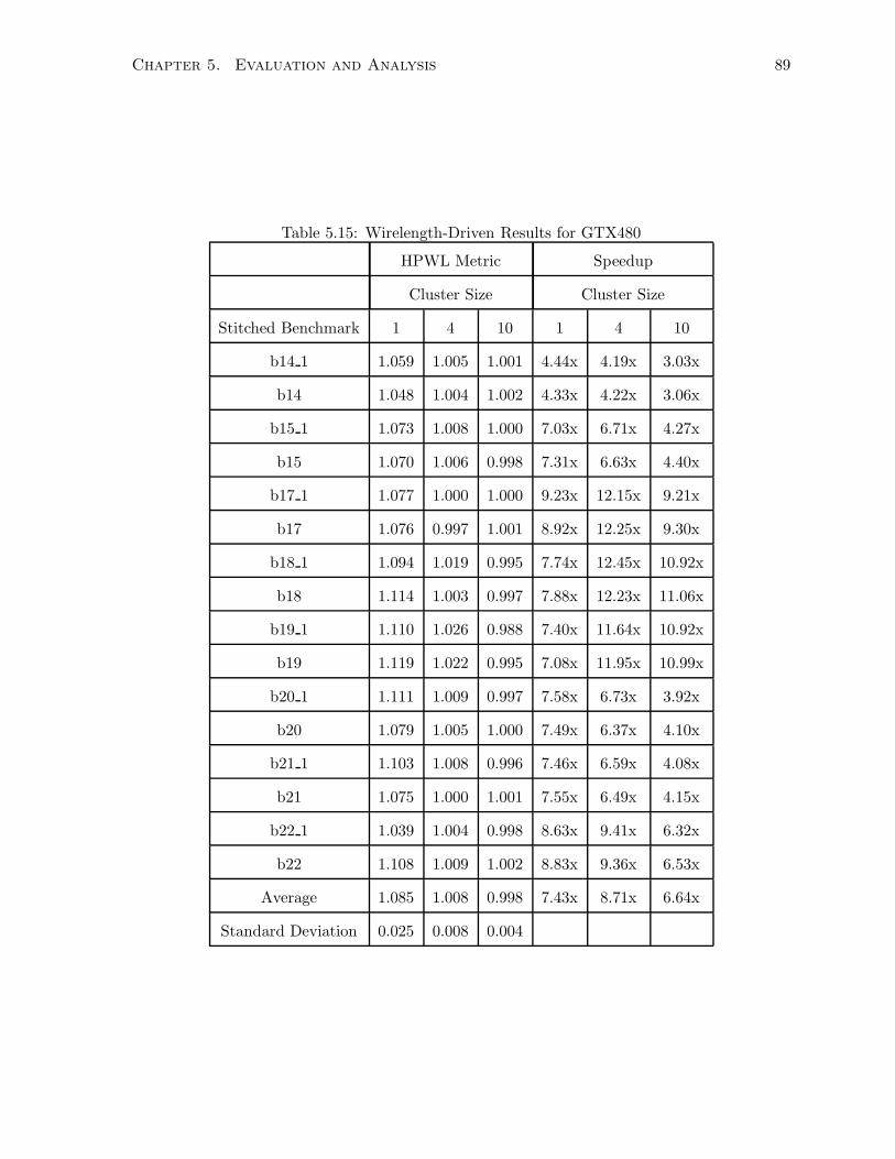
Chapter 5. Evaluation and Analysis 89
Table 5.15: Wirelength-Driven Results for GTX480
HPWL Metric Speedup
Cluster Size Cluster Size
Stitched Benchmark 1 4 10 1 4 10
b14 1 1.059 1.005 1.001 4.44x 4.19x 3.03x
b14 1.048 1.004 1.002 4.33x 4.22x 3.06x
b15 1 1.073 1.008 1.000 7.03x 6.71x 4.27x
b15 1.070 1.006 0.998 7.31x 6.63x 4.40x
b17 1 1.077 1.000 1.000 9.23x 12.15x 9.21x
b17 1.076 0.997 1.001 8.92x 12.25x 9.30x
b18 1 1.094 1.019 0.995 7.74x 12.45x 10.92x
b18 1.114 1.003 0.997 7.88x 12.23x 11.06x
b19 1 1.110 1.026 0.988 7.40x 11.64x 10.92x
b19 1.119 1.022 0.995 7.08x 11.95x 10.99x
b20 1 1.111 1.009 0.997 7.58x 6.73x 3.92x
b20 1.079 1.005 1.000 7.49x 6.37x 4.10x
b21 1 1.103 1.008 0.996 7.46x 6.59x 4.08x
b21 1.075 1.000 1.001 7.55x 6.49x 4.15x
b22 1 1.039 1.004 0.998 8.63x 9.41x 6.32x
b22 1.108 1.009 1.002 8.83x 9.36x 6.53x
Average 1.085 1.008 0.998 7.43x 8.71x 6.64x
Standard Deviation 0.025 0.008 0.004
Chapter 5. Evaluation and Analysis 90
in speedup across the two generations of GPUs is not 2x.
5.5 Summary
In this chapter, the evaluation methodology was described. Using this methodology, a sensitivity
analysis was performed on the parameters of the subset framework to gain an understanding of
how they impact quality of results and run time. A summary of the quality of results and run
time are provided for the wirelength-driven and timing-driven metric. Finally the determinism,
error tolerance and scalability of the framework are analyzed.
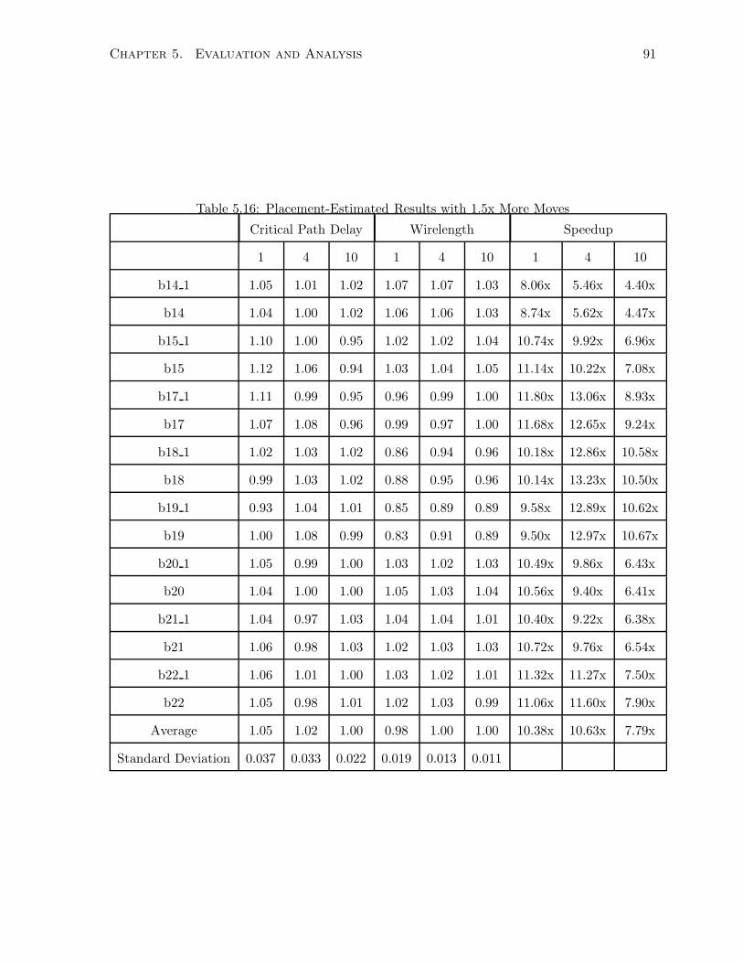
Chapter 5. Evaluation and Analysis 91
Table 5.16: Placement-Estimated Results with 1.5x More Moves
Critical Path Delay Wirelength Speedup
1 4 10 1 4 10 1 4 10
b14 1 1.05 1.01 1.02 1.07 1.07 1.03 8.06x 5.46x 4.40x
b14 1.04 1.00 1.02 1.06 1.06 1.03 8.74x 5.62x 4.47x
b15 1 1.10 1.00 0.95 1.02 1.02 1.04 10.74x 9.92x 6.96x
b15 1.12 1.06 0.94 1.03 1.04 1.05 11.14x 10.22x 7.08x
b17 1 1.11 0.99 0.95 0.96 0.99 1.00 11.80x 13.06x 8.93x
b17 1.07 1.08 0.96 0.99 0.97 1.00 11.68x 12.65x 9.24x
b18 1 1.02 1.03 1.02 0.86 0.94 0.96 10.18x 12.86x 10.58x
b18 0.99 1.03 1.02 0.88 0.95 0.96 10.14x 13.23x 10.50x
b19 1 0.93 1.04 1.01 0.85 0.89 0.89 9.58x 12.89x 10.62x
b19 1.00 1.08 0.99 0.83 0.91 0.89 9.50x 12.97x 10.67x
b20 1 1.05 0.99 1.00 1.03 1.02 1.03 10.49x 9.86x 6.43x
b20 1.04 1.00 1.00 1.05 1.03 1.04 10.56x 9.40x 6.41x
b21 1 1.04 0.97 1.03 1.04 1.04 1.01 10.40x 9.22x 6.38x
b21 1.06 0.98 1.03 1.02 1.03 1.03 10.72x 9.76x 6.54x
b22 1 1.06 1.01 1.00 1.03 1.02 1.01 11.32x 11.27x 7.50x
b22 1.05 0.98 1.01 1.02 1.03 0.99 11.06x 11.60x 7.90x
Average 1.05 1.02 1.00 0.98 1.00 1.00 10.38x 10.63x 7.79x
Standard Deviation 0.037 0.033 0.022 0.019 0.013 0.011
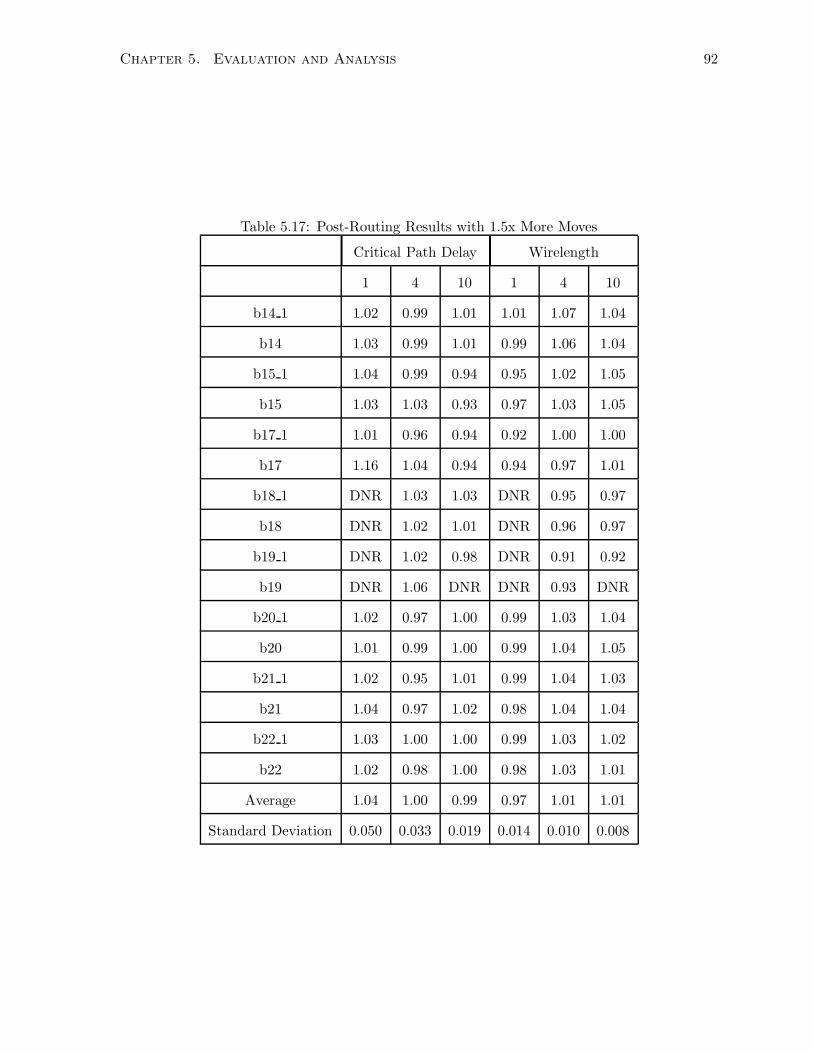
Chapter 5. Evaluation and Analysis 92
Table 5.17: Post-Routing Results with 1.5x More Moves
Critical Path Delay Wirelength
1 4 10 1 4 10
b14 1 1.02 0.99 1.01 1.01 1.07 1.04
b14 1.03 0.99 1.01 0.99 1.06 1.04
b15 1 1.04 0.99 0.94 0.95 1.02 1.05
b15 1.03 1.03 0.93 0.97 1.03 1.05
b17 1 1.01 0.96 0.94 0.92 1.00 1.00
b17 1.16 1.04 0.94 0.94 0.97 1.01
b18 1 DNR 1.03 1.03 DNR 0.95 0.97
b18 DNR 1.02 1.01 DNR 0.96 0.97
b19 1 DNR 1.02 0.98 DNR 0.91 0.92
b19 DNR 1.06 DNR DNR 0.93 DNR
b20 1 1.02 0.97 1.00 0.99 1.03 1.04
b20 1.01 0.99 1.00 0.99 1.04 1.05
b21 1 1.02 0.95 1.01 0.99 1.04 1.03
b21 1.04 0.97 1.02 0.98 1.04 1.04
b22 1 1.03 1.00 1.00 0.99 1.03 1.02
b22 1.02 0.98 1.00 0.98 1.03 1.01
Average 1.04 1.00 0.99 0.97 1.01 1.01
Standard Deviation 0.050 0.033 0.019 0.014 0.010 0.008
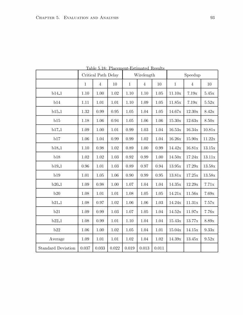
Chapter 5. Evaluation and Analysis 93
Table 5.18: Placement-Estimated Results
Critical Path Delay Wirelength Speedup
1 4 10 1 4 10 1 4 10
b14 1 1.10 1.00 1.02 1.10 1.10 1.05 11.10x 7.19x 5.45x
b14 1.11 1.01 1.01 1.10 1.09 1.05 11.85x 7.19x 5.52x
b15 1 1.32 0.99 0.95 1.05 1.04 1.05 14.67x 12.30x 8.42x
b15 1.18 1.06 0.94 1.05 1.06 1.06 15.30x 12.63x 8.50x
b17 1 1.09 1.00 1.01 0.99 1.03 1.04 16.53x 16.34x 10.81x
b17 1.06 1.04 0.99 0.99 1.02 1.04 16.26x 15.90x 11.22x
b18 1 1.10 0.98 1.02 0.89 1.00 0.99 14.42x 16.81x 13.15x
b18 1.02 1.02 1.03 0.92 0.99 1.00 14.50x 17.24x 13.11x
b19 1 0.96 1.01 1.03 0.89 0.97 0.94 13.95x 17.29x 13.58x
b19 1.01 1.05 1.06 0.90 0.99 0.95 13.81x 17.25x 13.58x
b20 1 1.09 0.98 1.00 1.07 1.04 1.04 14.35x 12.29x 7.71x
b20 1.08 1.01 1.01 1.08 1.05 1.05 14.21x 11.56x 7.69x
b21 1 1.08 0.97 1.02 1.06 1.06 1.03 14.24x 11.31x 7.57x
b21 1.09 0.99 1.03 1.07 1.05 1.04 14.52x 11.97x 7.76x
b22 1 1.08 0.99 1.01 1.10 1.04 1.04 15.43x 13.77x 8.89x
b22 1.06 1.00 1.02 1.05 1.04 1.01 15.04x 14.15x 9.33x
Average 1.09 1.01 1.01 1.02 1.04 1.02 14.39x 13.45x 9.52x
Standard Deviation 0.037 0.033 0.022 0.019 0.013 0.011
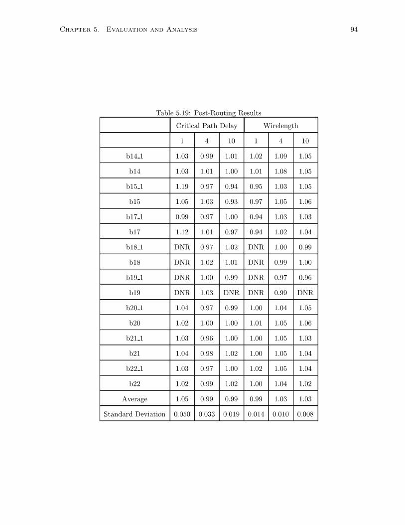
Chapter 5. Evaluation and Analysis 94
Table 5.19: Post-Routing Results
Critical Path Delay Wirelength
1 4 10 1 4 10
b14 1 1.03 0.99 1.01 1.02 1.09 1.05
b14 1.03 1.01 1.00 1.01 1.08 1.05
b15 1 1.19 0.97 0.94 0.95 1.03 1.05
b15 1.05 1.03 0.93 0.97 1.05 1.06
b17 1 0.99 0.97 1.00 0.94 1.03 1.03
b17 1.12 1.01 0.97 0.94 1.02 1.04
b18 1 DNR 0.97 1.02 DNR 1.00 0.99
b18 DNR 1.02 1.01 DNR 0.99 1.00
b19 1 DNR 1.00 0.99 DNR 0.97 0.96
b19 DNR 1.03 DNR DNR 0.99 DNR
b20 1 1.04 0.97 0.99 1.00 1.04 1.05
b20 1.02 1.00 1.00 1.01 1.05 1.06
b21 1 1.03 0.96 1.00 1.00 1.05 1.03
b21 1.04 0.98 1.02 1.00 1.05 1.04
b22 1 1.03 0.97 1.00 1.02 1.05 1.04
b22 1.02 0.99 1.02 1.00 1.04 1.02
Average 1.05 0.99 0.99 0.99 1.03 1.03
Standard Deviation 0.050 0.033 0.019 0.014 0.010 0.008
Chapter 6
Conclusion and Future Work
This thesis has demonstrated that the GPU, despite being optimized for streaming applications,
is capable of accelerating simulated annealing placement which is characterized by random
accesses to large memory. In fact, about an order of magnitude speedup is achieved with less
than 1% loss in quality of results on average for post-routed wirelength and less than no loss in
timing, except for cluster size of one which worsened by 4%. A cluster size of one is not used
in any FPGA architectures at the time of the writing of this thesis.
In accomplishing this, other findings are made
• Error can be tolerated. This work demonstrates that errors that arise when the decisions
are based on stale date do not significantly impact quality of results if controlled.
• The timing-driven metric of VPR can be transformed so that it utilizes less memory on
the GPU, and yet still maintains the quality of results for the critical path delay.
• While simulated annealing relies heavily on the random nature of move selection, it was
shown that move biasing weakly impacts quality of results. The advantage of biasing
moves is that it creates more opportunities to improve run time performance.
This work empirically investigated the impact of move biasing on quality of results and
performance. Future work could further explore the trade-offs associated with move biasing in
terms of quality of results and run time. This will allow designers of simulated annealing-based
tools to make more informed decisions when attempting to trade-off between speed and quality.
95
Bibliography
[1] Altera, “OpenCore stamping and benchmarking methodology,” Altera, Tech. Rep. TB-
098-1.1, 2008.
[2] S. Balachandran and D. Bhatia, “A-priori wirelength and interconnect estimation based
on circuit characteristics,” in SLIP ’03: Proceedings of the 2003 international workshop on
System-level interconnect prediction. New York, NY, USA: ACM, 2003, pp. 77–84.
[3] P. Banerjee, M. H. Jones, and J. S. Sargent, “Parallel simulated annealing algorithms for
cell placement on hypercube multiprocessors,” IEEE Trans. Parallel Distrib. Syst., vol. 1,
no. 1, pp. 91–106, 1990.
[4] BDTI, “BDTI focus report: FPGAs for DSP, second edition,” 2006,
http://www.bdti.com/products/reports fpga2006.html.
[5] V. Betz and J. Rose, “VPR: A new packing, placement and routing tool for FPGA re-
search,” in FPL ’97: Proceedings of the 7th International Workshop on Field-Programmable
Logic and Applications. London, UK: Springer-Verlag, 1997, pp. 213–222.
[6] V. Betz, J. Rose, and A. Marquardt, Eds., Architecture and CAD for Deep-Submicron
FPGAs. Norwell, MA, USA: Kluwer Academic Publishers, 1999.
[7] H. Bian, A. C. Ling, A. Choong, and J. Zhu, “Towards scalable placement for FPGAs,”
in FPGA ’10: Proceedings of the 18th annual ACM/SIGDA international symposium on
Field programmable gate arrays. New York, NY, USA: ACM, 2010, pp. 147–156.
[8] A. Casotto, F. Romeo, and A. Sangiovanni-Vincentelli, “A parallel simulated annealing
96
BIBLIOGRAPHY 97
algorithm for the placement of macro-cells,” Computer-Aided Design of Integrated Circuits
and Systems, IEEE Transactions on, vol. 6, no. 5, pp. 838–847, September 1987.
[9] V. Cerny, “A thermodynamical approach to the travelling salesman problem: An efficient
simulation algorithm,” Optimization Theory and Applications, vol. 45, no. 1, pp. 41–51,
January 1985.
[10] T. F. Chan, J. Cong, T. Kong, J. R. Shinnerl, and K. Sze, “An enhanced multilevel algo-
rithm for circuit placement,” in ICCAD ’03: Proceedings of the 2003 IEEE/ACM inter-
national conference on Computer-aided design. Washington, DC, USA: IEEE Computer
Society, 2003, p. 299.
[11] T. F. Chan, J. Cong, and E. Radke, “A rigorous framework for convergent net weighting
schemes in timing-driven placement,” in ICCAD ’09: Proceedings of the 2009 International
Conference on Computer-Aided Design. New York, NY, USA: ACM, 2009, pp. 288–294.
[12] S. Chatterjee, G. E. Blelloch, and M. Zagha, “Scan primitives for vector computers,” in
Supercomputing ’90: Proceedings of the 1990 ACM/IEEE conference on Supercomputing.
Los Alamitos, CA, USA: IEEE Computer Society Press, 1990, pp. 666–675.
[13] S. Chin and S. Wilton, “An analytical model relating fpga architecture and place and route
runtime,” aug. 2009, pp. 146 –153.
[14] A. Chowdhary, K. Rajagopal, S. Venkatesan, T. Cao, V. Tiourin, Y. Parasuram, and
B. Halpin, “How accurately can we model timing in a placement engine?” in DAC ’05:
Proceedings of the 42nd annual Design Automation Conference. New York, NY, USA:
ACM, 2005, pp. 801–806.
[15] W. E. Donath, R. J. Norman, B. K. Agrawal, S. E. Bello, S. Y. Han, J. M. Kurtzberg,
P. Lowy, and R. I. McMillan, “Timing driven placement using complete path delays,” in
DAC ’90: Proceedings of the 27th ACM/IEEE Design Automation Conference. New York,
NY, USA: ACM, 1990, pp. 84–89.
BIBLIOGRAPHY 98
[16] A. E. Dunlop, V. D. Agrawal, D. N. Deutsch, M. F. Jukl, P. Kozak, and M. Wiesel, “Chip
layout optimization using critical path weighting,” in DAC ’84: Proceedings of the 21st
Design Automation Conference. Piscataway, NJ, USA: IEEE Press, 1984, pp. 133–136.
[17] M. Durand, “Parallel simulated annealing: accuracy vs. speed in placement,” Design Test
of Computers, IEEE, vol. 6, no. 3, pp. 8 –34, jun. 1989.
[18] A. Kaufman, Z. Fan, and K. Petkov, “Implementing the lattice boltzmann
model on commodity graphics hardware,” Journal of Statistical Mechanics: The-
ory and Experiment, vol. 2009, no. 06, p. P06016, 2009. [Online]. Available:
http://stacks.iop.org/1742-5468/2009/i=06/a=P06016
[19] S. Kirkpatrick, C. D. Gelatt, and M. P. Vecchi, “Optimization by simulated annealing,”
Science, vol. 220, pp. 671–680, 1983.
[20] T. T. Kong, “A novel net weighting algorithm for timing-driven placement,” Computer-
Aided Design, International Conference on, vol. 0, pp. 172–176, 2002.
[21] S. A. Kravitz and R. A. Rutenbar, “Multiprocessor-based placement by simulated anneal-
ing,” in DAC ’86: Proceedings of the 23rd ACM/IEEE Design Automation Conference.
Piscataway, NJ, USA: IEEE Press, 1986, pp. 567–573.
[22] B. S. Landman and R. L. Russo, “On a pin versus block relationship for partitions of logic
graphs,” IEEE Trans. Comput., vol. 20, no. 12, pp. 1469–1479, 1971.
[23] A. Ludwin, V. Betz, and K. Padalia, “High-quality, deterministic parallel placement for
fpgas on commodity hardware,” in FPGA ’08: Proceedings of the 16th international
ACM/SIGDA symposium on Field programmable gate arrays. New York, NY, USA:
ACM, 2008, pp. 14–23.
[24] A. Marquardt, V. Betz, and J. Rose, “Timing-driven placement for FPGAs,” in FPGA
’00: Proceedings of the 2000 ACM/SIGDA eighth international symposium on Field pro-
grammable gate arrays. New York, NY, USA: ACM, 2000, pp. 203–213.
BIBLIOGRAPHY 99
[25] A. Mishchenko, S. Chatterjee, and R. Brayton, “Dag-aware aig rewriting a fresh look
at combinational logic synthesis,” in DAC ’06: Proceedings of the 43rd annual Design
Automation Conference. New York, NY, USA: ACM, 2006, pp. 532–535.
[26] G. E. Moore, “Cramming more components onto integrated circuits,” Electronics Maga-
zine, vol. 38, no. 8, pp. 114–117, April 1965.
[27] NVIDIA, “NVIDIA CUDA,” [online] http://www.nvidia.com/cuda.
[28] NVIDIA, “Nvidia cuda compute unified device arhcitecture programming guide: Version
2.0,” September 2009.
[29] H. Ren, “Sensitivity guided net weighting for placement driven synthesis,” in in Proc. Int.
Symp. on Physical Design, 2004, pp. 10–17.
[30] J. Rose, D. R. Blythe, W. M. Snelgrove, and Z. G. Vranesic, “Fast, high quality VLSI
placement on a MIMD multiprocessor,” Proc. Int. Conf. Computer-Aided Design, pp. 42–
45, 1986.
[31] ——, “Parallel standard cell placement algorithms with quality equivalent to simulated
annealing,” IEEE Trans. Computer-Aided Design, vol. 7, no. 3, pp. 387–396, 1988.
[32] C. Sechen and A. Sangiovanni-Vincentelli, “The TimberWolf placement and routing pack-
age,” Solid-State Circuits, IEEE Journal of, vol. 20, no. 2, pp. 510–522, Apr 1985.
[33] A. M. Smith, S. J. Wilton, and J. Das, “Wirelength modeling for homogeneous and hetero-
geneous FPGA architectural development,” in FPGA ’09: Proceeding of the ACM/SIGDA
international symposium on Field programmable gate arrays. New York, NY, USA: ACM,
2009, pp. 181–190.
[34] W.-J. Sun and C. Sechen, “A loosely coupled parallel algorithm for standard cell place-
ment,” in ICCAD ’94: Proceedings of the 1994 IEEE/ACM international conference on
Computer-aided design. Los Alamitos, CA, USA: IEEE Computer Society Press, 1994,
pp. 137–144.
BIBLIOGRAPHY 100
[35] W. Swartz and C. Sechen, “Timing driven placement for large standard cell circuits,” in
DAC ’95: Proceedings of the 32nd annual ACM/IEEE Design Automation Conference.
New York, NY, USA: ACM, 1995, pp. 211–215.
[36] R.-S. Tsay and J. Koehl, “An analytic net weighting approach for performance optimization
in circuit placement,” in DAC ’91: Proceedings of the 28th ACM/IEEE Design Automation
Conference. New York, NY, USA: ACM, 1991, pp. 620–625.
[37] E. E. Witte, R. D. Chamberlain, and M. A. Franklin, “Parallel simulated annealing using
speculative computation,” IEEE Trans. Parallel Distrib. Syst., vol. 2, no. 4, pp. 483–494,
1991.
[38] H. Wong, M.-M. Papadopoulou, M. Sadooghi-Alvandi, and A. Moshovos, “Demystifying
GPU microarchitecture through microbenchmarking,” in Performance Analysis of Systems
Software (ISPASS), 2010 IEEE International Symposium on, Mar. 2010, pp. 235 –246.
[39] M. Xu, G. Grewal, S. Areibi, C. Obimbo, and D. Banerji, “Near-linear wirelength estima-
tion for FPGA placement,” Electrical and Computer Engineering, Canadian Journal of,
vol. 34, no. 3, pp. 125 –132, 2009.