Mon. Not. R. Astron. Soc. 337, 1068–1080 (2002)

Parameter constraints for flat cosmologies from cosmic microwavebackground and 2dFGRS power spectra

Will J. Percival,1� Will Sutherland,1 John A. Peacock,1 Carlton M. Baugh,2

Joss Bland-Hawthorn,3 Terry Bridges,3 Russell Cannon,3 Shaun Cole,2 MatthewColless,4 Chris Collins,5 Warrick Couch,6 Gavin Dalton,7,8 Roberto De Propris,6

Simon P. Driver,9 George Efstathiou,10 Richard S. Ellis,11 Carlos S. Frenk,2 KarlGlazebrook,12 Carole Jackson,4 Ofer Lahav,10 Ian Lewis,3 Stuart Lumsden,13 SteveMaddox,14 Stephen Moody,9 Peder Norberg,2 Bruce A. Peterson4 and Keith Taylor3

(The 2dFGRS Team)1Institute for Astronomy, University of Edinburgh, Royal Observatory, Blackford Hill, Edinburgh EH9 3HJ2Department of Physics, University of Durham, South Road, Durham DH1 3LE3Anglo-Australian Observatory, PO Box 296, Epping, NSW 2121, Australia4Research School of Astronomy & Astrophysics, The Australian National University, Weston Creek, ACT 2611, Australia5Astrophysics Research Institute, Liverpool John Moores University, 12 Quays House, Birkenhead L14 1LD6Department of Astrophysics, University of New South Wales, Sydney, NSW 2052, Australia7Department of Physics, University of Oxford, Keble Road, Oxford OX1 3RH8Space Science and Technology Division, Rutherford Appleton Laboratory, Chilton, Didcot OX11 0QX9School of Physics and Astronomy, University of St Andrews, North Haugh, St Andrews, Fife KY6 9SS10Institute of Astronomy, University of Cambridge, Madingley Road, Cambridge CB3 0HA11Department of Astronomy, Caltech, Pasadena, CA 91125, USA12Department of Physics & Astronomy, Johns Hopkins University, Baltimore, MD 21218-2686, USA13Department of Physics, University of Leeds, Woodhouse Lane, Leeds LS2 9JT14School of Physics & Astronomy, University of Nottingham, Nottingham NG7 2RD

Accepted 2002 August 16. Received 2002 August 14; in original form 2002 July 1

ABSTRACTWe constrain flat cosmological models with a joint likelihood analysis of a new compilationof data from the cosmic microwave background (CMB) and from the 2dF Galaxy RedshiftSurvey (2dFGRS). Fitting the CMB alone yields a known degeneracy between the Hubbleconstant h and the matter density �m, which arises mainly from preserving the location ofthe peaks in the angular power spectrum. This ‘horizon-angle degeneracy’ is considered insome detail and is shown to follow the simple relation �m h3.4 = constant. Adding the 2dF-GRS power spectrum constrains �m h and breaks the degeneracy. If tensor anisotropies areassumed to be negligible, we obtain values for the Hubble constant of h = 0.665 ± 0.047,the matter density �m = 0.313 ± 0.055, and the physical cold dark matter and baryon densi-ties �c h2 = 0.115 ± 0.009, �b h2 = 0.022 ± 0.002 (standard rms errors). Including a possibletensor component causes very little change to these figures; we set an upper limit to the tensor-to-scalar ratio of r < 0.7 at a 95 per cent confidence level. We then show how these data canbe used to constrain the equation of state of the vacuum, and find w < −0.52 at 95 per centconfidence. The preferred cosmological model is thus very well specified, and we discuss theprecision with which future CMB data can be predicted, given the model assumptions. The2dFGRS power-spectrum data and covariance matrix, and the CMB data compilation usedhere, are available from http://www.roe.ac.uk/∼wjp/.

Key words: cosmic microwave background – cosmological parameters – large-scale structureof Universe.

�E-mail: wjp@roe.ac.uk

C© 2002 RAS

Parameter constraints for flat cosmologies 1069

1 I N T RO D U C T I O N

The 2dF Galaxy Redshift Survey (2dFGRS; see, e.g., Colless et al.2001) has mapped the local Universe in detail. If the galaxy dis-tribution has Gaussian statistics and the bias factor is independentof scale, then the galaxy power spectrum should contain all of theavailable information concerning the seed perturbations of cosmo-logical structure: it is statistically complete in the linear regime.The power spectrum of the data as of early 2001 was presentedin Percival et al. (2001), and was shown to be consistent with re-cent cosmic microwave background (CMB) and nucleosynthesisresults.

In Efstathiou et al. (2002) we combined the 2dFGRS power spec-trum with recent CMB data sets in order to constrain the cosmo-logical model (see also subsequent work by Lewis & Bridle 2002).Considering a wide range of possible assumptions, we were ableto show that the Universe must be nearly flat, requiring a non-zerocosmological constant �. The flatness constraint was quite pre-cise (|1 − �tot| < 0.05 at 95 per cent confidence); since inflationmodels usually predict near-exact flatness (|1 − �tot| < 0.001; e.g.Section 8.3 of Kolb & Turner 1990), there is strong empirical andtheoretical motivation for considering only the class of exactly flatcosmological models. The question of which flat universes matchthe data is thus an important one to be able to answer. Removingspatial curvature as a degree of freedom also has the practical ad-vantage that the space of cosmological models can be explored inmuch greater detail. Therefore, throughout this work we assume auniverse with baryons, cold dark matter (CDM) and vacuum energysumming to �tot = 1 (cf. Peebles 1984; Efstathiou, Sutherland &Maddox 1990).

In this work we also assume that the initial fluctuations wereadiabatic, Gaussian and well described by power-law spectra. Weconsider models with and without a tensor component, which is al-lowed to have slope and amplitude independent of the scalar compo-nent. Recent Sudbury Neutrino Observatory (SNO) measurements(Ahmad et al. 2002) are most naturally interpreted in terms of threeneutrinos of cosmologically negligible mass (�0.05 eV, as opposedto current cosmological limits of the order of 2 eV – see Elgaroyet al. 2002). We therefore assume zero neutrino mass in this analysis.In most cases, we assume the vacuum energy to be a ‘pure’ cosmo-logical constant with equation of state w ≡ p/ρc2 = −1, except inSection 5 where we explore w > −1.

In Section 2 we use a compilation of recent CMB observations(including data from VSA, Scott et al. 2002, and CBI, Pearson et al.2002, experiments) to determine the maximum-likelihood ampli-tude of the CMB angular power spectrum on a convenient grid,taking into account calibration and beam uncertainties where appro-priate. This compression of the data is designed to speed the analy-sis presented here, but it should be of interest to the community ingeneral.

In Section 3 we fit to both the CMB data alone, and CMB +2dFGRS. Fits to CMB data alone reveal two well-known primarydegeneracies. For models including a possible tensor component,there is tensor degeneracy (Efstathiou 2002) between increasingtensors, blue tilt, increased baryon density and lower CDM density.For both scalar-only and with-tensor models, there is a degener-acy related to the geometrical degeneracy present when non-flatmodels are considered, arising from models with similar observedCMB peak locations (cf. Efstathiou & Bond 1999). In Section 4 wediscuss this degeneracy further and explain how it may be easily un-derstood via the horizon angle, and described by the simple relation�m h3.4 = constant.

Section 5 considers a possible extension of our standard cosmo-logical model, allowing the equation of state parameter w of thevacuum energy component to vary. By combining the CMB data,the 2dFGRS data and an external constraint on the Hubble constanth, we are able to constrain w. Finally, in Section 6, we discuss therange of CMB angular power spectral values allowed by the presentCMB and 2dFGRS data within the standard class of flat models.

2 T H E C M B DATA

Recent key additions to the field of CMB observations come fromthe VSA (Scott et al. 2002), which boasts a smaller calibration er-ror than previous experiments, and the CBI (Pearson et al. 2002;Mason et al. 2002), which has extended observations to smaller an-gles (larger �). These data sets add to results from BOOMERaNG(Netterfield et al. 2002), Maxima (Lee et al. 2001) and DASI(Halverson et al. 2002), amongst others. Rather than compare mod-els with each of these data sets individually, it is expedient to com-bine the data prior to analysis. This combination often has the ad-vantage of allowing a consistency check between the individual datasets (e.g. Wang, Tegmark & Zaldarriaga 2002). However, care mustbe taken to ensure that additional biases are not introduced into thecompressed data set, and that no important information is lost.

In the following we consider COBE, BOOMERaNG, Max-ima, DASI, VSA and CBI data sets. The BOOMERaNG data ofNetterfield et al. (2002) and the Maxima data of Lee et al. (2001)were used assuming the data points to be independent, and havewindow functions well described by top-hats. The � < 2000 CBImosaic field data were used assuming that the only significant cor-relations arise between neighbouring points that are anticorrelatedat the 16 per cent level as discussed in Pearson et al. (2002). Win-dow functions for these data were assumed to be Gaussian withsmall negative side lobes extending into neighbouring bins approxi-mately matched to fig. 11 of Pearson et al. (2002). We also considerthe VSA data of Scott et al. (2002), the DASI data of Halversonet al. (2002), and the COBE data compilation of Tegmark (1996),for which the window functions and covariance matrices are known,where appropriate. The calibration uncertainties used are presentedin Table 1, and the data sets are shown in Fig. 1. In total, there aresix data sets, containing 68 power measurements.

In order to combine these data sets, we have fitted a model forthe true underlying CMB power spectrum, consisting of power val-ues at a number of � values (or nodes). Between these nodes weinterpolate the model power spectrum using a smooth Spline3 algo-rithm (Press et al. 1992). The assumption of smoothness is justifiedbecause we aim to compare CMB data with CDM models calcu-lated using CMBFAST (Seljak & Zaldarriaga 1996). Internally, this

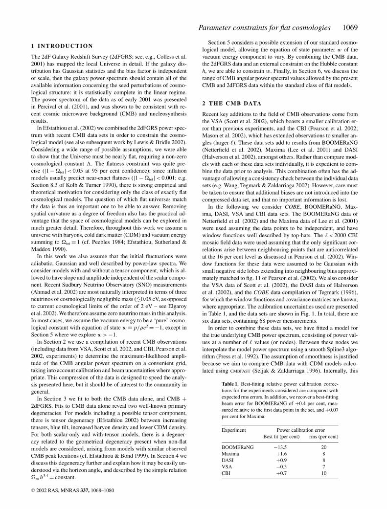
Table 1. Best-fitting relative power calibration correc-tions for the experiments considered are compared withexpected rms errors. In addition, we recover a best-fittingbeam error for BOOMERaNG of +0.4 per cent, mea-sured relative to the first data point in the set, and +0.07per cent for Maxima.

Experiment Power calibration errorBest fit (per cent) rms (per cent)

BOOMERaNG −13.5 20Maxima +1.6 8DASI +0.9 8VSA −0.3 7CBI +0.7 10

C© 2002 RAS, MNRAS 337, 1068–1080

1070 W. J. Percival et al.

Figure 1. Top panel: the compilation of recent CMB data used in our analysis (see the text for details). The solid line shows the result of a maximum-likelihoodfit to these data, allowing for calibration and beam uncertainty errors in addition to intrinsic errors. Each observed data set has been shifted by the appropriatebest-fitting calibration and beam correction. Bottom panel: the solid line again shows our maximum-likelihood fit to the CMB power spectrum now showingthe nodes (the points at which the amplitude of the power spectrum was estimated) with approximate errors calculated from the diagonal elements of thecovariance matrix (solid squares). These data are compared with the compilation of Wang et al. (2002) (stars) and the result of convolving our best-fitting powerwith the window function of Wang et al. (crosses). In order to show the important features in the CMB angular power spectrum plots we present in this paperwe have chosen to scale the x-axis by (log �)5/2.

code evaluates the CMB power spectrum only at a particular set of� values, which are subsequently Spline3 interpolated to cover allmultipoles. It is therefore convenient to use as our parameters theCMB power values at the same nodes used by CMBFAST in the keyregime 150 � � � 1000. Using the same smoothing algorithm andnodes for our estimate of the true power spectrum, we ensure that noadditional assumptions are made in the data compilation comparedwith the models to be tested. For � < 150 and � > 1000 the datapoints are rather sparsely distributed, and we only selected a few� values at which to estimate the power. The best-fitting amplitudeof the power spectrum at an extra node at � = 2000 was determinedin our fit to the observed CMB data, in order for the shape of the in-terpolated curve around � = 1500 to have the correct form. This wassubsequently removed from the analysis, and models and data wereonly compared for � � 1500. In addition to requiring no interpola-tion in CMBFAST, this method of compression has a key advantage forour analysis. Normally, CMB data are expressed as bandpowers, inwhich one specifies the result of convolving the CMB power spec-trum with some kernel. This remains true of some previous CMB

data compilations (e.g. Wang et al. 2002). In contrast, we estimatethe true power spectrum at a given � directly, so that no convolutionstep is required. This means that parameter space can be exploredmore quickly and efficiently.

Given a set of nodal values, we form an interpolated model powerspectrum, convolve with the window function of each observed datapoint and maximized the likelihood with respect to the nodal val-ues (assuming Gaussianity – see Bond, Jaffe & Knox 2000 for adiscussion of the possible effect of this approximation). Calibrationerrors and beam uncertainties were treated as additional independentGaussian parameters, and were combined into the final likelihood,as well as being used to correct the data. The resulting best-fittingcalibration and beam errors are compared with the expected rmsvalues in Table 1.

In agreement with Wang et al. (2002), we find a negative best-fitting BOOMERaNG calibration correction (13 per cent in power),caused by matching data sets in the regime 300 < � < 500. Applyingthis correction (included in the data points in Fig. 1) slightly de-creases the amplitude of the first peak. Nevertheless, our combined

C© 2002 RAS, MNRAS 337, 1068–1080

Parameter constraints for flat cosmologies 1071

Table 2. Recovered best-fitting power spec-trum values with rms values given the six datasets analysed.

� δT 2 (µK2) rms error (µK2)

2 314 4434 803 2268 770 156

15 852 17450 1186 141490 2796 673

150 3784 546200 5150 627250 5306 590300 3407 364350 2339 265400 1627 205450 1873 202500 2214 240550 2479 249600 2061 245650 1849 244700 2023 274750 1614 295800 2089 373850 2654 475900 2305 515950 1178 480

1000 1048 3201200 1008 2141500 530 178

power values are systematically higher than in the compilation ofWang et al. (see the lower panel of Fig. 1). This derives partly fromthe inclusion of extra data, but also results from a bias in the analysismethod of Wang et al. They use the observed power values to esti-mate the error in the data, rather than the true power at that multipole(which we estimate from our model). A low observational point isthus given a spuriously low error, and this is capable of biasing theaveraged data to low values.

The final best-fitting power spectrum amplitudes given the sixdata sets analysed are presented in Table 2, with the correspond-ing �-values of the nodes and rms errors. Formally, this fit gaveχ 2

min = 31.9, given 34 degrees of freedom (there are 68 data points,and we estimate 27 power spectrum values, five calibration andtwo beam corrections). This result demonstrates that the differentdata sets are broadly consistent after allowing for calibration andbeam uncertainty. The Hessian matrix of the likelihood provides anestimate of the inverse covariance matrix for the power spectrum es-timates. This was calculated numerically and is available, togetherwith the averaged data, from http://www.roe.ac.uk/∼wjp/. As em-phasized previously, these are estimates of the true power at the� values given and therefore do not require window functions. Inthe following section we use these CMB results to constrain flatcosmological models.

3 C O S M O L O G I C A L M O D E L S

3.1 Parameter space

In the following we parametrize flat cosmological models with sevenparameters (plus two amplitudes): these are the physical baryon den-

Table 3. The distribution of parameters (defined in the text)in the ∼ 2 × 108 flat cosmological models considered in thispaper. The grid used was linear in each parameter between thelimits given in order to simplify the marginalization assuminga uniform prior on each.

Parameter Min Max Grid size

�bh2 0.01 0.04 25�ch2 0.05 0.22 25h 0.40 1.00 25τ 0.00 0.10 2ns 0.80 1.30 25nt −0.20 0.30 10r 0.00 1.00 25

sity1 �b h2, the physical CDM density �c h2, the Hubble constant h,the optical depth to the last scattering surface τ , the scalar spectralindex ns, the tensor spectral index nt and the tensor-to-scalar ratio r.The tensor-to-scalar ratio r is defined as in Efstathiou et al. (2002):the scalar and tensor C� are normalized so that

1

4π

1000∑�=2

(2� + 1)CS� = (4 × 10−5)2, (1)

1

4π

50∑�=2

(2� + 1)CT� = (2 × 10−5)2. (2)

C� is then given by C� = Q2(CS� + rCT

� ), where Q2 is the nor-malization constant. We marginalize over both this and the ampli-tude of the 2dFGRS power spectra in order to avoid complicationscaused by galaxy biasing and redshift space distortions (Lahav et al.2002).

CMB angular power spectra have been calculated using CMBFAST

(Seljak & Zaldarriaga 1996) for a grid of ∼ 2 × 108 models. Forease of use, a uniform grid was adopted with a varying resolution ineach of the parameters (details of this grid are presented in Table 3).Likelihoods were calculated by fitting these models to the reducedCMB data set presented in Section 2. Similarly, large-scale structure(LSS) power spectra were calculated for the relevant models usingthe fitting formula of Eisenstein & Hu (1998), and were convolvedwith the window function of the 2dFGRS sample, before beingcompared with the 2dFGRS data as in Percival et al. (2001).

In order to constrain parameters, we wish to determine the prob-ability of each model in our grid given the available CMB and 2dF-GRS data. However, we can only easily calculate the probability ofthe data given each model. In order to convert between these prob-abilities using Bayes’ theorem, we need to adopt a prior probabilityfor each model or parameter. In this work, we adopt a uniform priorfor the parameters discussed above between the limits in Table 3. i.e.we assume that the prior probability of each model in the grid is thesame. Assuming a uniform prior for physically motivated parame-ters is common in the field, although not often explicitly mentioned.Note that the constraints placed by the current data are tight com-pared with the prior, and that the biases induced by this choice aretherefore relatively small.

The likelihood distribution for a single parameter, or for twoparameters can be calculated by marginalizing the estimated

1 As usual, �b and �c are the densities of baryons and CDM in units of thecritical density, and h is the Hubble constant in units of 100 km s−1 Mpc−1.‘Derived’ parameters include the matter density �m = �c + �b and�� = 1 − �m.

C© 2002 RAS, MNRAS 337, 1068–1080

1072 W. J. Percival et al.

Figure 2. Two parameter likelihood surfaces for scalar-only models. Contours correspond to changes in the likelihood from the maximum of2� lnL= 2.3, 6.0, 9.2. Dashed contours are calculated by only fitting to the CMB data, solid contours by jointly fitting the CMB and 2dFGRS data. Dottedlines show the extent of the grid used to calculate the likelihoods.

probability of the model given the data over all other parameters. Be-cause of the grid adopted in this work, we can perform this marginal-ization by simply averaging the L values calculated at each point inthe grid.

In Fig. 2 we present two-parameter likelihood contour plots(marginalized over the remaining parameters) for the subset ofscalar-only models, i.e. r fixed at 0. For these scalar-only models,we choose to plot τ only against �b h2 as τ is poorly constrainedby the CMB data, and has no degeneracies with the other param-eters. In Fig. 3 we present two-parameter likelihood contour plots(marginalized over the remaining parameters) for models allowinga tensor component. The spectral index of the tensor contribution ispoorly constrained by the CMB data so, as for τ , we only show oneplot with this parameter.

Figs 2 and 3 reveal two key directions in parameter space that theCMB data have difficulty constraining. When a tensor componentis included, we have the tensor degeneracy – a trade-off betweenincreasing tensors, increasing ns, increasing �b h2 and decreasing�c h2 (for more detail see Efstathiou 2002). In addition, in both thescalar-only and with-tensor cases, there is a degeneracy between�c h2 and h, which results in the Hubble parameter h being poorlyconstrained by the CMB data alone. This degeneracy is discussedin detail in the next section.

We note that nearly all of the likelihood is contained well withinour prior regions, except for the case of tensor models with CMB-only data in Fig. 3: here there is a region allowed by CMB outsideour priors with high tensor fraction, h > 1, ns � 1.3, �c h2 � 0.06.These parameters are ruled out by many observations apart from2dFGRS, so the truncation is not a concern.

3.2 Results

The recovered mean and standard rms error calculated for each pa-rameter (except τ which is effectively unconstrained) are given in

Table 4. What is striking is how well specified many of the param-eters are.

The general features are as follows: changing from the compila-tion of Wang et al. to our compilation shrinks the error bars slightly(owing to VSA and CBI), but the central values are similar exceptfor a slight shift in ns. Allowing tensors widens the error bars andcauses modest shifts in central values (the best fit has a zero tensorfraction, but the fact that r must be non-negative explains the shifts).The CMB data alone constrains �b h2 and ns well and �c h2 quitewell, but �m and h less well. Adding the 2dFGRS data shrinks theerrors on �c h2, h and thus �m and �b/�m by more than a factorof 2.

The most restrictive case is the set of scalar-only models. Theseyield h = 0.665 with only a 7 per cent error, which is substantiallybetter than any other method. The matter density parameter comesout at �m = 0.313, with a rather larger error of 18 per cent; errorson h and �m are anticorrelated so the physical matter density is welldetermined,�m h2 = 0.136 ± 7 per cent. In Section 4 below we showthat this is because the CMB data measure the combination �m h3

very accurately, so that an accurate measurement of �m requiresh to be known almost exactly.

Moving from matter content to the fluctuation spectrum,the scalar-only results give a tantalizing hint of red tilt, withns = 0.963 ± 0.042. Current data are thus within a factor of 2 of theprecision necessary to detect plausible degrees of tilt (e.g. ns = 0.95for λφ4 inflation; see Section 8.3 of Liddle & Lyth 2000). Inflationof course cautions against ignoring tensors, but it would be a greatstep forward to rule out an ns = 1 scalar-only model.

Including the possibility of tensors changes these conclusionsonly moderately. The errors on h and �m hardly alter, whereas theerror on ns rises to 0.066. The preferred model has r = 0, althoughthis is rather poorly constrained. Marginalizing over the other pa-rameters, we obtain a 95 per cent confidence upper limit of r < 0.7.One way of ruling out the upper end of this range may be to note that

C© 2002 RAS, MNRAS 337, 1068–1080

Parameter constraints for flat cosmologies 1073

Figure 3. As in Fig. 2, but now considering a wider class of models that possibly include a tensor component.

such tensor-dominated models predict a rather low normalization forthe present-day mass fluctuations, as we now discuss.

3.3 Normalization

An advantage of the new CMB data included here is that the mostrecent experiments have a rather small calibration uncertainty. It istherefore possible to obtain precise values for the overall normal-ization of the power spectrum. As usual, we take this to be specifiedby σ8, the rms density contrast averaged over spheres of 8 h−1 Mpcradius. For the scalar-only grid of models shown in Fig. 2, thisyields

σ8 = (0.72 ± 0.03 ± 0.02) exp(τ ). (3)

The first error figure is the ‘theory error’: the uncertainty in σ8

that arises because the conversion between the observed C� and thepresent P(k) depends on the uncertain values of �m, etc. The seconderror figure represents the uncertainty in the normalization of the C�

data (see Fig. 7 in Section 6). The total error in σ8 is the sum inquadrature of these two figures.

This result confirms with greater precision our previous conclu-sions that the allowed scalar-only models prefer a relatively lownormalization (Efstathiou et al. 2002; Lahav et al. 2002). As dis-

cussed by Lahav et al. (2002), a figure of σ8 = 0.72 is consistentwith the relatively wide range of estimates from the abundance ofrich clusters, but is lower than the σ8 � 0.9 for �m � 0.3 preferredby weak lensing studies. The obvious way to reconcile these figuresis via the degenerate dependence of σ8 on τ . The lowest plausiblevalue for this is τ = 0.05, corresponding to reionization at zr = 8 forthe parameters given here. To achieve σ8 = 0.9 requires τ = 0.22, orreionization at zr = 22, which is somewhat higher than conventionalestimates (zr < 15; see, e.g., Loeb & Barkana 2001). Additional ev-idence in this direction comes from the possible first detection ofSunyaev–Zeldovich anisotropies at � > 200 by the CBI (Mason et al.2002). This signal is claimed to require σ8 � 1 (Bond et al. 2002),which would raise zr to almost 30. Further scrutiny of these indepen-dent estimates for σ8 will be required before one can claim evidencefor first object formation at extreme redshifts, but this is an excitingpossibility.

Finally, we note that these problems are sharpened if the CMBpower spectrum has a substantial tensor component. As shown byEfstathiou et al. (2002), the model with the maximal allowed tensorfraction (r = 0.6) has a normalization lower by a factor 1.18 than thebest scalar-only model. This pushes zr to almost 40 for σ8 = 1, whichstarts to become implausibly high, even given the large uncertaintiesassociated with the modelling of reionization.

C© 2002 RAS, MNRAS 337, 1068–1080

1074 W. J. Percival et al.

Table 4. The recovered mean and root mean square (rms) error for each parameter, calculated by marginalizing overthe remaining parameters. Results are presented for scalar-only and scalar + tensor models, and for CMB data only orCMB and 2dFGRS power spectrum data. To reduce round-off error, means and rms errors are quoted to an accuracysuch that the rms error has two significant figures. We also present constraints on some of the possible derived parametercombinations. (Note that because of the marginalization, the maximum-likelihood values of ‘derived’ parameters, e.g.�m are not simply ratios of the ML values for each ‘independent’ parameter.)

Parameter Results: scalar only Results: with tensor componentCMB CMB + 2dFGRS CMB CMB + 2dFGRS

�bh2 0.0205 ± 0.0022 0.0210 ± 0.0021 0.0229 ± 0.0031 0.0226 ± 0.0025�ch2 0.118 ± 0.022 0.1151 ± 0.0091 0.100 ± 0.023 0.1096 ± 0.0092

h 0.64 ± 0.10 0.665 ± 0.047 0.75 ± 0.13 0.700 ± 0.053Using the ns 0.950 ± 0.044 0.963 ± 0.042 1.040 ± 0.084 1.033 ± 0.066CMB data nt − − 0.09 ± 0.16 0.09 ± 0.16compilation r − − 0.32 ± 0.23 0.32 ± 0.22of Section 2 �m 0.38 ± 0.18 0.313 ± 0.055 0.25 ± 0.15 0.275 ± 0.050

�mh 0.226 ± 0.069 0.206 ± 0.023 0.174 ± 0.063 0.190 ± 0.022�mh2 0.139 ± 0.022 0.1361 ± 0.0096 0.123 ± 0.022 0.1322 ± 0.0093

�b/�m 0.152 ± 0.031 0.155 ± 0.016 0.193 ± 0.048 0.172 ± 0.021

�bh2 0.0209 ± 0.0022 0.0216 ± 0.0021 0.0233 ± 0.0032 0.0233 ± 0.0025�ch2 0.124 ± 0.024 0.1140 ± 0.0088 0.107 ± 0.025 0.1091 ± 0.0089

h 0.64 ± 0.11 0.682 ± 0.046 0.74 ± 0.14 0.719 ± 0.054Using the ns 0.987 ± 0.047 1.004 ± 0.047 1.073 ± 0.087 1.079 ± 0.073Wang et al. (2002) nt − − 0.03 ± 0.15 0.03 ± 0.15compilation r − − 0.25 ± 0.21 0.27 ± 0.20

�m 0.41 ± 0.20 0.296 ± 0.051 0.28 ± 0.17 0.261 ± 0.048�mh 0.240 ± 0.076 0.200 ± 0.021 0.189 ± 0.071 0.185 ± 0.021�mh2 0.145 ± 0.024 0.1356 ± 0.0092 0.131 ± 0.024 0.1324 ± 0.0088

�b/�m 0.149 ± 0.033 0.160 ± 0.016 0.186 ± 0.049 0.177 ± 0.021

4 T H E H O R I Z O N A N G L E D E G E N E R AC Y

In this section we explore the degeneracy observed in Figs 2 and 3between �c h2 and h. This is related (but not identical) to the geomet-rical degeneracy that exists when non-flat models are considered,and we now show that it is very closely related to the location ofthe acoustic peaks. Below, we first review the basics of the geo-metrical degeneracy; secondly, note why this is only weakly brokenby the flatness assumption, and thirdly give a simple heuristic ar-gument why this degeneracy approximately follows a contour ofnearly constant �m h3.

4.1 The geometrical degeneracy

The ‘geometrical degeneracy’ in the CMB is well known (Bond,Efstathiou & Tegmark 1997; Zaldarriaga, Spergel & Seljak 1997;Efstathiou & Bond 1999). If we take a family of models withfixed initial perturbation spectra, fixed physical densities ωm ≡�m h2, ωb ≡ �b h2, and vary both �� and the curvature �k to keep afixed value of the angular size distance to last scattering, then the re-sulting CMB power spectra are identical (except for the integratedSachs–Wolfe effect at low multipoles, which is hidden in cosmicvariance, and second-order effects at high �). This degeneracy oc-curs because the physical densities ωm, ωb control the structure ofthe perturbations in physical Mpc at last scattering, while curvatureand � (plus ωm) govern the proportionality between the length atlast scattering and the observed angle. Note that h is a ‘derived’parameter in the above set, via h = [ωm/(1 − �k − ��)]1/2, so thegeometrical degeneracy is broken by an external measurement of h.

4.2 The flat-universe case

Assuming a flat universe, �k = 0, thus also breaks the geometricaldegeneracy. However, as noted by, for example, Efstathiou & Bond

(1999), and investigated below, there is a closely related degeneracybased on varying two free parameters (chosen from �m, ωm, h, ��)so as to almost preserve the locations of the first few CMB acousticpeaks. This is illustrated in Fig. 4, where the likelihood contoursin the (�m, h) plane for CMB-only data form a long and narrow‘banana’ with its long axis at approximately constant �m h3. Thebanana is surprisingly narrow in the other direction; this means that�m h3 is determined to approximately 12 per cent (1σ ) by the CMBdata.

This ‘banana’ is similar in form to the line in fig. 4 of Efstathiou& Bond (1999), though it is different in detail because they usedsimulations with ωm = 0.25. It is also similar to that in fig. 1 ofKnox, Christensen & Skordis (2001) as expected. However, bothof those previous papers presented the degeneracy in the (��, h)plane; although this is just a mirror-image of the (�m, h) plane,it is less intuitive (e.g. changing �� alters observables that haveno explicit � dependence, via the constraint �m = 1 − ��), so thesimple �m h3 dependence has not been widely recognized.

4.3 Peak locations and the sound horizon

The locations �m of the first few CMB acoustic peaks may be con-veniently expressed (e.g. Hu et al. 2001; Knox et al. 2001) as

�m = �A(m − φm), m = 1, 2, 3 (4)

�A ≡ π/θS (5)

θS ≡ rS(z∗)

DA(z∗), (6)

where rS is the sound horizon size at last scattering (redshift z∗),DA is the angular diameter distance to last scattering, therefore θS

is the ‘sound horizon angle’ and �A is the ‘acoustic scale’. For any

C© 2002 RAS, MNRAS 337, 1068–1080

Parameter constraints for flat cosmologies 1075

Figure 4. Likelihood contours for �m against h for scalar-only models,plotted as in Fig. 2. Variables were changed from �bh2 and �ch2 to �m

and �b/�m, and a uniform prior was assumed for �b/�m covering thesame region as the original grid. The extent of the grid is shown by thedotted lines. The dot-dashed line follows the locus of models throughthe likelihood maximum with constant �mh3.4. The solid line is a fit tothe likelihood valley and shows the locus of models with constant �mh3.0

(see the text for details).

given model, the CMB peak locations �m(m = 1, 2, 3) are given bynumerical computation, and then equation (4) defines the empiri-cal ‘phase shift’ parameters φm. Hu et al. (2001) show that the φm

are weakly dependent on cosmological parameters and φ1 ∼ 0.27,φ2 ∼ 0.24, φ3 ∼ 0.35. Extensive calculations of the φm are given byDoran & Lilley (2002).

Therefore, although θS is not directly observable, it is very simpleto compute and very tightly related to the peak locations, henceits use below. Knox et al. (2001) note a ‘coincidence’ that θS istightly correlated with the age of the universe for flat models withparameters near the ‘concordance’ values, and use this to obtain anaccurate age estimate assuming flatness.

4.4 A heuristic explanation

Here we provide a simple heuristic explanation for why θS andhence the �ms are primarily dependent on the parameter combination�m h3.4.

Of the four ‘FRW’ parameters �m, ωm, h, ��, only two are inde-pendent for flat models, and we can clearly choose any pair exceptfor (�m, ��). The standard choice in CMB analyses is (ωm, ��),while for non-CMB work the usual choice is (�m, h). However, inthe following we take ωm and �m to be the independent parameters(thus h, �� are derived); this looks unnatural but separates moreclearly the low-redshift effect of �m from the pre-recombination ef-fect of ωm. We take ωb as fixed unless otherwise specified (its effecthere is small).

We first note that the present-day horizon size for flat models iswell approximated by (Vittorio & Silk 1985)

rH(z = 0) = 2c

H0�−0.4

m = 6000 Mpc�0.1

m√ωm

. (7)

(The distance to last scattering is ∼ 2 per cent smaller than theabove because of the finite redshift of last scattering.) Therefore,if we increase �m while keeping ωm fixed, the shape and relativeheights of the CMB peaks are preserved but the peaks move slowlyrightwards (increasing �) proportional to �0.1

m . (Equivalently, theEfstathiou–Bond R parameter for flat models is well approximatedby 1.94 �0.1

m .)This slow variation of �A ∝ �0.1

m at fixed ωm explains why thegeometrical degeneracy is only weakly broken by the restriction toflat models: a substantial change in �m at fixed ωm moves the peaksonly slightly, so a small change in ωm can alter the sound horizonlength rS(z∗) and bring the peaks back to their previous angularlocations with only a small change in relative heights. We now givea simplified argument for the dependence of rS on ωm.

The comoving sound horizon size at last scattering is defined by(e.g. Hu & Sugiyama 1995)

rS(z∗) ≡ 1

H0�1/2m

∫ a∗

0

cS

(a + aeq)1/2da, (8)

where the vacuum energy is neglected at these high redshifts; theexpansion factor a ≡ (1 + z)−1 and a∗, aeq are the values at recombi-nation and matter–radiation equality, respectively. Thus rS dependson ωm and ωb in several ways:

(i) the expansion rate in the denominator depends on ωm via aeq;(ii) the speed of sound cS depends on the baryon/photon ratio via

cS = c/√

3(1 + R), R = 30 496 ωb a;(iii) the recombination redshift z∗ depends on both the baryon

and matter densities ωb, ωm in a fairly complex way.

Since we are interested mainly in the derivatives of rS with ωm, ωb,it turns out that (i) above is the dominant effect. The dependence(iii) of z∗ on ωm, ωb is slow. Concerning (ii), for baryon densi-ties ωb � 0.02, cS declines smoothly from c/

√3 at high redshift to

0.80 c/√

3 at recombination. Therefore, to a reasonable approxi-mation we may take a fixed ‘average’ cS � 0.90 c/

√3 outside the

integral in equation (8), and take a fixed z∗, giving the approximation

rS(z∗) � 0.90√3

rH (z = 1100), (9)

where rH is the light horizon size; this approximation is very accuratefor all ωm considered here and ωb � 0.02. For other baryon densities,multiplying the right-hand side of equation (9) by (ωb/0.02)−0.07 isa refinement. [Around the concordance value ωb = 0.02, effects (ii)and (iii) partly cancel, because increasing ωb lowers the speed ofsound but also delays recombination i.e. increases a∗.]

From above, the (light) horizon size at recombination is

rH(z∗) = c

H0�1/2m

∫ a∗

0

1

(a + aeq)1/2da

= 6000 Mpc√ωm

√a∗

[√1 + (aeq/a∗) −

√aeq/a∗

]. (10)

Dividing by DA � 0.98 rH (z = 0) from equation (7) gives the anglesubtended today by the light horizon,

θH � 1.02�−0.1

m√1 + z∗

(√1 + aeq

a∗−

√aeq

a∗

). (11)

Inserting z∗ = 1100 and aeq = (23 900 ωm)−1, we have

θH = 1.02 �−0.1m√

1101

×[√

1 + 0.313

(0.147

ωm

)−

√0.313

(0.147

ωm

)], (12)

C© 2002 RAS, MNRAS 337, 1068–1080

1076 W. J. Percival et al.

and θS � θH × 0.9/√

3 from equation (9). This remarkably simpleresult captures most of the parameter dependence of CMB peaklocations within flat �CDM models. Note that the square bracketsin equation (12) tends (slowly) to 1 for aeq � a∗ i.e. ωm � 0.046;thus it is the fact that matter domination occurred not much earlierthan recombination that leads to the significant dependence of θH

on ωm and hence h.Differentiating equation (12) near a fiducial ωm = 0.147 gives

∂ ln θH

∂ ln �m

∣∣∣∣ωm

= −0.1,

∂ ln θH

∂ ln ωm

∣∣∣∣�m

= 1

2

(1 + a∗

aeq

)−1/2

= +0.24, (13)

and the same for derivatives of ln θS from the approximation above.In terms of (�m, h) this gives

∂ ln θH

∂ ln �m

∣∣∣∣h

= +0.14,∂ ln θH

∂ ln h

∣∣∣∣�m

= +0.48, (14)

in good agreement with the numerical derivatives of �A in equa-tion (A15) of Hu et al. (2001). Also note the sign difference betweenthe two ∂/∂ ln �m values above.

Thus for moderate variations from a ‘fiducial’ model, theCMB peak locations scale approximately as �m ∝ �−0.14

m h−0.48, i.e.the condition for constant CMB peak location is well approxi-mated as �m h3.4 = constant. This condition can also be written asωm�−0.41

m = constant, and we see that, along such a contour, ωm

varies as �0.41m , and hence the peak heights are slowly varying and

the overall CMB power spectrum is also slowly varying.There are four approximations used for θS above: one in equa-

tion (7), two (constant cs and z∗) in equation (9), and finally the�m h3.4 line is a first-order (in log) approximation to a contour ofconstant equation (12). Checking against numerical results, we findthat each of these causes up to 1 per cent error in θS, but theypartly cancel: the exact value of θS varies by <0.5 per cent alongthe contour h = 0.7(�m/0.3)−1/3.4 between 0.1 ��m � 1. The peakheights shift the numerical degeneracy by more than this (see below),so the error is unimportant.

A line of constant �m h3.4 is compared with the likelihood surfacerecovered from the CMB data in Fig. 4. In order to calculate the re-quired likelihoods, we have made a change of variables from ωb and�c h2 to �m and �b/�m, and have marginalized over the baryonfraction assuming a uniform prior in �b/�m covering the limits ofthe grid used. As expected, the degeneracy observed when fitting theCMB data alone is close to a contour of constant �A and hence con-stant θH. However, information concerning the peak heights does al-ter this degeneracy slightly; the relative peak heights are preserved atconstant ωm, hence the actual likelihood ridge is a ‘compromise’ be-tween constant peak location (constant�m h3.4) and constant relativeheights (constant �m h2); the peak locations have more weight in thiscompromise, leading to a likelihood ridge along �m h3.0 � constant.This is shown by the solid line in Fig. 4. To demonstrate where thisalteration is coming from, we have plotted three scalar-only mod-els in the top panel of Fig. 5. These models lie approximately alongthe line of constant �m h3.4, with �m = 0.93, 0.36, 0.10. Parametersother than �m and h have been adjusted to fit the CMB data. The dif-fering peak heights (especially the third peak) between the modelsare clear (though not large) and the data therefore offer an additionalconstraint that slightly alters the observed degeneracy. The bottompanel of Fig. 5 shows three models that lie along the observed de-generacy, again with �m = 0.93, 0.36, 0.11. The narrow angle of

intersection between contours of constant �m h3.4 and �m h2 [only10◦ in the (ln �m, ln h) plane] explains why the likelihood bananais long.

The exponent of h for constant θH varies slowly from 2.9 to 4.1as ωm varies from 0.06 to 0.26. Note that Hu et al. (2001) quote anexponent of 3.8 for constant �1; the difference from 3.4 is mainlycaused by the slight dependence of φ1 on ωm, which we ignoredabove. However, since that paper, improved CMB data has betterrevealed the second and third peaks, and the exponent of 3.4 ismore appropriate for preserving the mean location of the first threepeaks. Also, note that the near-integer exponent of 3.0 for the like-lihood ridge in Fig. 4 is a coincidence that depends on the observedvalue of ωm, details of the CMB error bars, etc. However, the argu-ments above are fairly generic, so we anticipate that any CMB dataset covering the first few peaks should (assuming flatness) give alikelihood ridge elongated along a contour of constant �m h p , withp fairly close to 3.

To summarize this section, the CMB peak locations are closely re-lated to the angle subtended by the sound horizon at recombination,which we showed is a near-constant fraction of the light horizonangle given in equation (12). We have thus called this the ‘horizonangle degeneracy’, which has more physical content than the alter-native ‘peak location degeneracy’. A contour of constant θS is verywell approximated by a line of constant �m h3.4, and informationon the peak heights slightly ‘rotates’ the measured likelihood ridgenear to a contour of constant �m h3.0.

5 C O N S T R A I N I N G QU I N T E S S E N C E

There has been recent interest in a possible extension of the stan-dard cosmological model that allows the equation of state of thevacuum energy w ≡ pvac/ρvacc2 to have w �= −1 (e.g. Zlatev, Wang& Steinhardt 1999), thereby not being a ‘cosmological constant’,but a dynamically evolving component. In this section we extendour analysis to constrain models with w �−1; we assume w doesnot vary with time since a model with time-varying w generallylooks very similar to a model with a suitably chosen constant w

(e.g. Kujat et al. 2002). The shapes of the CMB and matter powerspectra are invariant to changes of w (assuming the vacuum energywas negligible before recombination): the only significant effect isto alter the angular diameter distance to last scattering, and movethe angles at which the acoustic peaks are seen. For flat models, auseful approximation to the present-day horizon size is given by

rH(z = 0) = 2c

H0�−α

m , α = −2w

1 − 3.8w(15)

(compare with equation 7 for w = −1). As discussed previously, theprimary constraint from the CMB data is on the angle subtended to-day by the light horizon (given for w = −1 models by equation 12).If w is increased from −1 at fixed �m, h, the peaks in the CMBangular power spectrum move to larger angles. To continue to fitthe CMB data, we must decrease �m h3.4 to bring θH back to its‘best-fitting’ value. However, the 2dFGRS power spectrum con-straint limits �mh = 0.20 ± 0.03, so to continue to fit both CMB +2dFGRS we must reduce h.

The CMB and 2dFGRS data sets alone therefore constrain a com-bination of w and h, but not both separately. The dashed lines inFig. 6 show likelihood contours for w against h fitting to both theCMB and 2dFGRS power spectra showing this effect. Here, we havemarginalized over �m assuming a uniform prior 0.0 < �m < 1.3.An extra constraint on h can be converted into a limit on w: if we

C© 2002 RAS, MNRAS 337, 1068–1080

Parameter constraints for flat cosmologies 1077

Figure 5. The top panel shows three scalar-only model CMB angular power spectra with the same apparent horizon angle, compared with the data of Table 1.Although these models have approximately the same value of �m h3.4, they are distinguishable by peak heights. Such additional constraints alter the degeneracyobserved in Fig. 4 slightly from �m h3.4 to �m h3.0. Three scalar-only models that lie in the likelihood ridge with �m h3.0 are compared with the data in thebottom panel. For all of the models shown, parameters other than �m and h have been adjusted to their maximum-likelihood positions.

include the measurement h = 0.72 ± 0.08 from the Hubble SpaceTelescope (HST) key project (Freedman et al. 2001) we obtain thesolid likelihood contours in Fig. 6. The combination of these threedata sets then gives w < −0.52 (95 per cent confidence); the limit ofthe range considered, w = −1.0, provides the smallest uncertainty.The 95 per cent confidence limit is comparable to the w < −0.55 ob-tained from the supernova Hubble diagram plus flatness (Garnavichet al. 1998). See also Efstathiou (1999), who obtained w < −0.6from a semi-independent analysis combining CMB and supernovae(again assuming flatness).

6 P R E D I C T I N G T H E C M B P OW E R S P E C T RU M

An interesting aspect of this analysis is that the current CMB dataare rather inaccurate for 20 � � � 100, and yet the allowed CDMmodels are strongly constrained. We therefore consider how wellthis model-dependent determination of the CMB power spectrum isdefined, in order to see how easily future data could test the basicCDM + flatness paradigm.

Using our grid of ∼ 2 × 108 models, we have integrated the CMB+ 2dFGRS likelihood over the range of parameters presented inTable 3 in order to determine the mean and rms CMB power at

each �. These data are presented in Table 5 at selected � values, andthe range of spectra is shown by the grey-shaded region in the toppanel of Fig. 7. A possible tensor component was included in thisanalysis, although this has a relatively minor effect, increasing theerrors slightly (as expected when new parameters are introduced),but hardly affecting the mean values. The predictions are remarkablytight: this is partly because combining the peak-location constrainton �m h3.4 with the 2dFGRS constraint on �mh gives a better con-straint on �m h2 than the CMB data alone, and this helps to constrainthe predicted peak heights.

The bottom panel of Fig. 7 shows the errors on an expanded scale,compared with the cosmic variance limit and the predicted errorsfor the MAP experiment (Page 2002). This comparison shows that,while MAP will beat our present knowledge of the CMB angularpower spectrum for all � � 800, this will be particularly apparentaround the first peak. As an example of the issues at stake, the scalar-only models predict that the location of the first CMB peak shouldbe at � = 221.8 ± 2.4. Significant deviations observed by MAP fromsuch predictions will imply that some aspect of this model (or thedata used to constrain it) is wrong. Conversely, if the observations ofMAP are consistent with this band, then this will be strong evidencein favour of the model.

C© 2002 RAS, MNRAS 337, 1068–1080

1078 W. J. Percival et al.

Table 5. The predicted mean and rms CMBpower calculated by integrating the CMB +2dFGRS likelihood over the range of param-eters presented in Table 3, allowing for a pos-sible tensor component. These data form atestable prediction of the CDM + flatnessparadigm.

� δT 2 (µK2) rms error (µK2)

2 920 1344 817 1028 775 8815 828 9650 1327 10090 2051 87150 3657 172200 4785 186250 4735 150300 3608 113350 2255 82400 1567 52450 1728 79500 2198 86550 2348 74600 2052 76650 1693 51700 1663 79750 1987 131800 2305 122850 2257 93900 1816 107950 1282 931000 982 461200 1029 691500 686 60

Figure 6. Likelihood contours for the equation of state of the vacuum energyparameter w against the Hubble constant h. Dashed contours are for CMB+ 2dFGRS data, solid contours include also the HST key project constraint.Contours correspond to changes in the likelihood from the maximum of2� lnL= 2.3, 6.0, 9.2. Formally, this results in a 95 per cent confidencelimit of w < −0.52.

7 S U M M A RY A N D D I S C U S S I O N

Following recent releases of CMB angular power spectrum measure-ments from VSA and CBI, we have produced a new compilation ofdata that estimates the true power spectrum at a number of nodes,assuming that the power spectrum behaves smoothly between thenodes. The best-fitting values are not convolved with a window func-tion, although they are not independent. The data and Hessian matrixare available from http://www.roe.ac.uk/∼wjp/CMB/. We have usedthese data to constrain a uniform grid of ∼ 2 × 108 flat cosmologicalmodels in seven parameters jointly with 2dFGRS large-scale struc-ture data. By fully marginalizing over the remaining parameters wehave obtained constraints on each, for the cases of CMB data alone,and CMB + 2dFGRS data. The primary results of this paper are theresulting parameter constraints, particularly the tight constraints onh and the matter density �m: combining the 2dFGRS power spec-trum data of Percival et al. (2001) with the CMB data compilationof Section 2, we find h = 0.665 ± 0.047 and �m = 0.313 ± 0.055(standard rms errors), for scalar-only models, or h = 0.700 ± 0.053and �m = 0.275 ± 0.050, allowing a possible tensor component.

We have also discussed in detail how these parameter constraintsarise. Constraining �tot = 1 does not fully break the geometrical de-generacy present when considering models with varying �tot, andmodels with CMB power spectra that peak at the same angular posi-tion remain difficult to distinguish using CMB data alone. A simplederivation of this degeneracy was presented, and models with con-stant peak locations were shown to closely follow lines of constant�m h3.4. We can note a number of interesting phenomenologicalpoints from this analysis.

(i) The narrow CMB �m–h likelihood ridge in Fig. 4 derives pri-marily from the peak locations, therefore it is insensitive to many ofthe parameters affecting peak heights, e.g. tensors, ns, τ , calibrationuncertainties, etc. Of course it is strongly dependent on the flatnessassumption.

(ii) This simple picture is broken in detail as the current CMBdata obviously place additional constraints on the peak heights. Thischanges the degeneracy slightly, leading to a likelihood ridge nearconstant �m h3.

(iii) The high power of h3 means that adding an external h con-straint is not very powerful in constraining �m, but an external �m

constraint gives strong constraints on h. A 10 per cent measurementof �m (which may be achievable, for example, from evolution ofcluster abundances) would give a 4 per cent measurement of h.

(iv) When combined with the 2dF power spectrum shape(which mainly constrains �mh), the CMB + 2dFGRS datagives a constraint on �m h2 = 0.1322 ± 0.0093 (including ten-sors) or �m h2 = 0.1361 ± 0.0096 (scalars only), which is con-siderably tighter from the CMB alone. Subtracting the baryonsgives �c h2 = 0.1096 ± 0.0092 (including tensors) or �c h2 =0.1151 ± 0.0091 (scalars only), accurate results that may be valuablein constraining the parameter space of particle dark matter modelsand thus predicting rates for direct-detection experiments.

(v) We can understand the solid contours in Fig. 4 simplyas follows: the CMB constraint can be approximated as a one-dimensional stripe �m h3.0 = 0.0904 ± 0.0092 (including tensors)or �m h3.0 = 0.0876 ± 0.0085 (scalars only), and the 2dF con-straint as another stripe �mh = 0.20 ± 0.03. Multiplying two Gaus-sians with the above parameters gives a result that looks quitesimilar to the fully marginalized contours. In fact, modellingthe CMB constraint simply using the location of the peaksto give �m h3.4 = 0.081 ± 0.012 (including tensors) or �m h3.4 =

C© 2002 RAS, MNRAS 337, 1068–1080

Parameter constraints for flat cosmologies 1079

Figure 7. Upper panel: the grey-shaded region shows our prediction of the CMB angular power spectrum with 1σ errors (see the text); points show the data ofTable 1. The lower panel shows fractional errors: points are the current data, dashed line is the errors on our prediction, and the three solid lines are expectederrors for the MAP experiment (Page 2002) for �� = 50 and the 6-month, 2- and 4-yr data (top to bottom). The dotted line shows the expected cosmic variance,again for �� = 50, assuming full sky coverage (the MAP errors assume 80 per cent coverage). As can be seen, the present CMB and LSS data provide a strongprediction over the full �-range covered by MAP.

0.073 ± 0.010 (scalars only) also produces a similar result, demon-strating that the primary constraint of the CMB data in the (�m, h)plane is on the apparent horizon angle.

In principle, accurate non-CMB measurements of both �m andh can give a robust prediction of the peak locations assuming flat-ness. If the observed peak locations are significantly different, thiswould give evidence for either non-zero curvature, quintessencewith w �= −1 or some more exotic failure of the model. Using theCMB data to constrain the horizon angle, and 2dFGRS data to con-strain �mh, there remains a degeneracy between w and h. This can bebroken by an additional constraint on h; using h = 0.72 ± 0.08 fromthe HST key project (Freedman et al. 2001), we find w < −0.52 at95 per cent confidence. This result is comparable to that found byEfstathiou (1999) who combined the supernovae sample ofPerlmutter et al. (1999) with CMB data to find w < −0.6.

In Section 6 we considered the constraints that combining theCMB and 2dFGRS data place on the CMB angular power spectrum.This was compared with the predicted errors from the MAP satellitein order to determine where MAP will improve on the present dataand provide the strongest constraints on the cosmological model.

It will be fascinating to see whether MAP rejects these predictions,thus requiring a more complex cosmological model than the simplestflat CDM-dominated universe.

Finally, we announce the public release of the 2dFGRS powerspectrum data and associated covariance matrix determined byPercival et al. (2001). We also provide code for the numerical cal-culation of the convolved power spectrum and a window matrix forthe fast calculation of the convolved power spectrum at the data val-ues. The data are available from either http://www.roe.ac.uk/∼wjp/or from http://www.mso.anu.edu.au/2dFGRS; as we have demon-strated, they are a critical resource for constraining cosmologicalmodels.

AC K N OW L E D G M E N T S

The 2dF Galaxy Redshift Survey was made possible through thededicated efforts of the staff of the Anglo-Australian Observatory,both in creating the 2dF instrument and in supporting it on thetelescope.

C© 2002 RAS, MNRAS 337, 1068–1080

1080 W. J. Percival et al.

R E F E R E N C E S

Ahmad Q. et al., 2002, Phys. Rev. Lett., 89, 011301Bond J.R., Efstathiou G., Tegmark M., 1997, MNRAS, 291, L33Bond J.R., Jaffe A.H., Knox L., 2000, ApJ, 533, 19Bond J.R. et al., 2002, ApJ, submitted (astro-ph/0205386)Colless M. et al., 2001, MNRAS, 328, 1039Doran M., Lilley M., 2002, MNRAS, 330, 965Efstathiou G., 1999, MNRAS, 310, 842Efstathiou G., 2002, MNRAS, 332, 193Efstathiou G., Bond J.R., 1999, MNRAS, 304, 75Efstathiou G., Sutherland W., Maddox S., 1990, Nat, 348, 705Efstathiou G. et al., 2002, MNRAS, 330, 29Eisenstein D.J., Hu W., 1998, ApJ, 496, 605Elgaroy O. et al., 2002, Phys. Rev. Lett., 89, 061301Freedman W.L. et al., 2001, ApJ, 553, 47Garnavich P.M. et al., 1998, ApJ, 509, 74Halverson N.W. et al., 2002, ApJ, 568, 38Hu W., Sugiyama N., 1995, ApJ, 444, 489Hu W., Fukugita M., Zaldarriaga M., Tegmark M., 2001, ApJ, 549, 669Knox L., Christensen N., Skordis C., 2001, ApJ, 563, L95Kolb E.W., Turner M.S., 1990, The Early Universe. Addison-Wesley,

Reading, MAKujat J., Linn A.M., Scherrer R.J., Weinberg D.H., 2002, ApJ, 572, 1Lahav O. et al., 2002, MNRAS, 333, 961Lee A.T. et al., 2001, ApJ, 561, L1

Lewis A., Bridle S., 2002, Phys. Rev. D submitted (astro-ph/0205436)Liddle A.R., Lyth D.H., 2000, Cosmological Inflation and Large-Scale Struc-

ture. Cambridge Univ. Press, CambridgeLoeb A., Barkana R., 2001, ARAA, 39, 19Mason B.S. et al., 2002, ApJ, submitted (astro-ph/0205384)Netterfield C.B. et al., 2002, ApJ, 571, 604Page L., 2002, in Sato K., Shiromizu T., eds, New Trends in Theoretical

and Observational Cosmology. Universal Academy Press, Tokyo (astro-ph/0202145)

Peacock J.A. et al., 2001, Nat, 410, 169Pearson T.J. et al., 2002, ApJ, submitted (astro-ph/0205388)Peebles P.J.E., 1984, ApJ, 284, 444Percival W.J. et al., 2001, MNRAS, 327, 1297Perlmutter S. et al., 1999, ApJ, 517, 565Press W.H., Teukolsky S.A., Vetterling W.T., Flannery B.P., 1992, Numerical

Recipes in C, 2nd edn. Cambridge Univ. Press, CambridgeScott P.F. et al., 2002, MNRAS, submitted (astro-ph/0205380)Seljak U., Zaldarriaga M., 1996, ApJ, 469, 437Tegmark M., 1996, ApJ, 464, L35Vittorio N., Silk J., 1985, ApJ, 297, L1Wang X., Tegmark M., Zaldarriaga M., 2002, Phys. Rev. D, 65, 123001Zaldarriaga M., Spergel D.N., Seljak U., 1997, ApJ, 488, 1Zlatev I., Wang L., Steinhardt P.J., 1999, Phys. Rev. Lett., 82, 896

This paper has been typeset from a TEX/LATEX file prepared by the author.

C© 2002 RAS, MNRAS 337, 1068–1080