Parameter estimation and regionalization for continuous

rainfall-runoff models including uncertainty

Thorsten Wagenera,*, Howard S. Wheaterb

aDepartment of Civil and Environmental Engineering, 226B Sackett Bldg., Pennsylvania State University, University Park, PA 16801, USAbDepartment of Civil and Environmental Engineering, Imperial College London, SW7 2BU, London, UK

Abstract

The prediction of streamflow at ungauged sites is one of the fundamental challenges to hydrologists today. While major

progress has been made in the regionalization of statistical flow properties (e.g. extreme values), and methods for synthesis of

event response at ungauged sites are widely applied, the estimation of continuous streamflow time-series is still very uncertain.

The challenge of predicting the response at ungauged sites is often met through a process of parameter regionalization. Little

attention has so far been given to the impact of new insights into model identification at gauged sites, e.g. regarding the problem

of structural error, on this regionalization process. Questions that are addressed in this paper are the following: (1) What is the

relationship between local parameter identifiability and catchment characteristics? (2) How is the uniqueness of catchments

reflected in regionalization? (3) What is the result of local model structural uncertainty on the regionalization result? (4) How

can we propagate local parameter uncertainty into predictions in ungauged basins and what is the result? A case study of 10

catchments located in the southeast of England is utilized to deal with these questions. The main conclusions from this study are

that the uncertainty in the locally estimated model parameters is a function of their importance in representing the response of a

given catchment, model structural error hinders identification of a parameter to represent a certain process and therefore hinders

the regionalization, and the uncertainty in the calibrated parameters can be propagated to ungauged sites using a weighted

regression approach.

q 2005 Elsevier Ltd. All rights reserved.

Keywords: Rainfall-runoff modelling; Ungauged catchments; Regionalization; Parameter estimation; Uncertainty; Model structural error

1. Introduction

Rainfall-runoff (RR) models are commonly used

tools to extrapolate streamflow time-series in time and

space for operational and scientific investigations. RR

models allow, for example, to extend available

streamflow records in time to predict the behavior of

0022-1694/$ - see front matter q 2005 Elsevier Ltd. All rights reserved.

doi:10.1016/j.jhydrol.2005.07.015

* Corresponding author. Tel.: C1 814 865 5673; fax: C1 814 863

7304.

catchments for different climate scenarios. Through

extrapolation in space, they enable us to simulate the

response of catchments for which little or no time-

series of streamflow measurements are available. The

latter has been achieved with some success in terms of

predicting the response of a catchment to an

individual rainfall event, using (parametrically)

simple models (e.g. Natural Environment Research

Council NERC, 1975; McCuen, 1982). However,

water resource and flood management hydrological

Journal of Hydrology 320 (2006) 132–154

www.elsevier.com/locate/jhydrol

T. Wagener, H.S. Wheater / Journal of Hydrology 320 (2006) 132–154 133

problems are increasingly approached using continu-

ous time RR modelling (e.g. Lamb, 2000; Cameron et

al., 2001; Blazkova and Beven, 2002; Lamb and Kay,

2004), rather than traditional statistical or event-based

models (e.g. NERC, 1975; Pilgrim, 1983; Houghton-

Carr, 1999). The reliable estimation of continuous

streamflow time-series in ungauged catchments has

remained a largely unsolved problem so far (Wagener

et al., 2004), although significant insights have been

gained in recent years as discussed below. The

establishment of the Prediction in Ungauged Basins

(PUB) initiative by the International Association of

Hydrological Sciences (IAHS) shows that much has

still to be done in this area (Sivapalan et al., 2003;

Wagener et al., 2004).

Many, if not most, RR model structures currently

used for continuous modelling can be classified as

conceptual (CRR), if the classification is based on two

criteria (Wheater et al., 1993): (1) the structure of

these models is specified prior to any modelling being

undertaken, and (2) (at least some of) the model

parameters do not have a direct physical interpret-

ation, in the sense of being independently measurable,

and have to be estimated through calibration against

observed data. Calibration is a process of parameter

adjustment (automatic or manual), until catchment

and model behavior show a sufficiently (to be

specified by the hydrologist) high degree of similarity.

The similarity is usually judged by one or more

objective functions (OFs) accompanied by visual

inspection of observed and calculated hydrographs

(Gupta et al., 2004). It is usually assumed that the

model parameters represent some inherent and time-

invariant properties of the catchment under study.

Early attempts to model ungauged catchments

simply used the parameter values derived for

neighboring catchments where streamflow data were

available, i.e. a geographical proximity approach (e.g.

Mosley, 1981; Vandewiele and Elias, 1995). How-

ever, this seems to be insufficient since even nearby

catchments can be very different with respect to their

hydrological behavior (Post et al., 1998; Beven,

2000). Others propose the use of parameter estimates

directly derived from, amongst others, soil properties

such as porosity, field capacity and wilting point (to

derive model storage capacity parameters); percen-

tage forest cover (evapotranspiration parameters); or

hydraulic conductivities and channel densities (time

constants) (e.g. Koren et al., 2000; Duan et al., 2001;

Atkinson et al., 2002). The main problem here is that

the scale at which the measurements are made (often

from small soil samples) is different from the scale at

which the model equations are derived (often

laboratory scale) and at which the model is usually

applied (catchment scale). The conceptual model

parameters represent the effective characteristics of

the integrated (heterogeneous) catchment system

(including for example preferential flow), which are

unlikely to be easily captured using small-scale

measurements since there is generally no theory that

allows the estimation of the effective values within

different parts of a heterogeneous flow domain from a

limited number of small scale or laboratory measure-

ments (Beven et al., 2000). It seems unlikely that

conceptual model parameters, which describe an

integrated catchment response, usually aggregating

significant heterogeneity (including the effect of

preferential flow paths, different soil and vegetation

types, etc.), can be derived from catchment properties

that do not consider all influences on water flow

through the catchment. Further fine-tuning of these

estimates using locally observed flow data is needed

because the physical information available to estimate

a priori parameters is not adequate to define local

physical properties of individual basins for accurate

hydrologic forecasts (Duan et al., 2001). However,

useful initial values might be derived in this way

(Koren et al., 2000). The advantages of this approach

are that the assumed physical basis of the parameters

is preserved and that (physical) parameter dependence

can be accounted for, as shown by Koren et al. (2000).

Probably the most common approach to ungauged

modelling is to relate model parameters and catch-

ment characteristics in a statistical manner (e.g.

Jakeman et al., 1992; Sefton et al., 1995; Post et al.,

1998; Sefton and Howarth, 1998; Abdullah and

Lettenmaier, 1997; Wagener et al., 2004; Merz and

Bloschl, 2004; Lamb and Kay, 2004; Seibert, 1999;

Lamb et al., 2000; Post and Jakeman, 1996;

Fernandez et al., 2000), assuming that the uniqueness

of each catchment can be captured in a unique

combination of catchment characteristics. The basic

methodology is to calibrate a specific model structure,

here called the local model structure, to as large a

number of (gauged) catchments as possible and derive

statistical (regression) relationships between (local)

T. Wagener, H.S. Wheater / Journal of Hydrology 320 (2006) 132–154134

model parameters and catchment characteristics.

These statistical relationships, here called regional

models, and the measurable properties of the

ungauged catchment can then be used to derive

estimates of the (local) model parameters. This

procedure is usually referred to as regionalization or

spatial generalization (e.g. Lamb and Calver, 2002).

This paper addresses both theoretical and applied

issues related to the regionalization of continuous

lumped and parsimonious (parameter efficient) CRR

models. The principle of parameter regionalization is

discussed, and current problems and possible direc-

tions of improvement are identified and evaluated

using 10 catchments located in the southeast of

England. The objective is not to derive reliable

regional model equations, which is unlikely to be

robust with the small number of catchments used, but

to investigate the effect of parameter and model

structure identification issues on the regionalization of

lumped CRR models. The Model Parameter Esti-

mation Experiment (MOPEX) includes a variety of

researchers who apply a statistical regionalization

approach. Here we test underlying assumptions

commonly made in this method and their impact on

the results.

2. Model regionalization—procedure

and uncertainties

Any RR model can be written in the following

simplified form (Wagener et al., 2004),

Q Z MLðqLjIÞC3L (1)

where Q is the simulated streamflow, I is a matrix of

input variables (e.g. rainfall and temperature), ML is a

given (local) model structure, qL is a vector of

parameters within this structure and 3L is an error

term. The model parameters will usually be estimated

through calibration if measured time-series of runoff

over a sufficiently long period are available. The

required length of the time-series depends, amongst

other things, on the complexity of the model structure

used and the information content of the available data.

It might range from 3 years (Sefton and Howarth,

1998; Jakeman and Hornberger, 1993) for a simple

model structure, to up to about a decade for a more

complex one (Yapo et al., 1996). However, in

principle, the data set should always be sufficiently

long to avoid the problem of the parameters only

being representative of a particular climate period

(Gan and Burges, 1990).

If no runoff data are available for a specific

catchment, i.e. if it is ungauged, an attempt can be

made to calibrate the model structure to a large

number of gauged catchments and to find a functional

relationship between the (usually individual) concep-

tual model parameters (dependent variables) and the

catchment characteristics (independent variables), i.e.

a regional model structure of the following type:

qL Z HRðqRjFÞCyR (2)

where qL is the estimated model parameter at the

ungauged site, HR($) is a functional relation for qL

using a set of physiographic and meteorological

catchment characteristics F, while qR is a set of

regional model parameters and nR is an error term.

One model, i.e. (regional) model structure and

(regional) parameter combination is conventionally

derived for each (local) parameter, i.e. the model

parameters are assumed to be independent. The

regional model structure commonly takes the form

of a linear or a non-linear regression equation.

No generally accepted procedure for regionaliza-

tion of conceptual, continuous model parameters

currently exists. However, the following steps are

typically found and are therefore given here as the

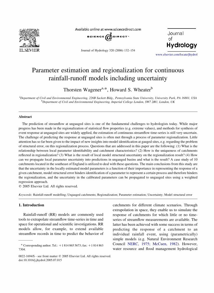
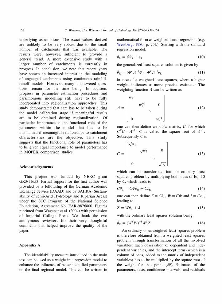
basic outline of a regionalization procedure (Fig. 1):

Decide which (sub-)set of catchments can be

described by a single local model structure ML

and a single regional model, i.e. one structure HR

with a specific set of parameters qR. Catchments

that are very different with respect to their

dominant hydrological processes might require

different (local) model structures to represent them

in a physically (or probably rather conceptually)

realistic manner. This segmentation of catchments

must be related to the catchment characteristics Fin order to classify any ungauged catchment.

Appropriate characteristics could be size, drainage

density, soils/geology, land use, etc.

Apply the local model structure ML to each of the

gauged catchments and estimate the optimum

LOCALMODEL

STRUCTURE

GAUGEDCATCHMENT 1

GAUGEDCATCHMENT 2

GAUGEDCATCHMENT N

REGIONALMODEL

STRUCTURE

UNGAUGEDCATCHMENT*

Q*

I*

θ*

Φ*

I 1

θ1

I2

θ2

IN

θN

θ1,Φ

1

θ2,Φ2

θ N,ΦN

Fig. 1. Schematic representation of a regionalization procedure.

T. Wagener, H.S. Wheater / Journal of Hydrology 320 (2006) 132–154 135

parameter set (or population) qL for each catch-

ment.

Relate the derived (individual) parameter values

qLi and the catchment characteristics F using the

regional model structure HRi. Apply the regional

model HRiðqRijFÞ to estimate each parameter qLi

for the ungauged catchment.

Predict flow in the ungauged catchment using

parameter set qL.

Each of the steps outlined above introduces

uncertainties that are unavoidably propagated into

the regionalization result (the streamflow prediction at

an ungauged site). They can be categorized into two

groups, first, uncertainties related to local modelling

(i.e. those related to the selection and calibration of

the local model structure to each catchment), and

second, uncertainties related to the procedure for

spatial extrapolation using a regional model. The

main uncertainties are:

Selection of catchment properties, i.e. what are

suitable characteristics to describe and cluster

(pool) catchments with respect to their hydro-

logical response? This is important for both the

local and the regional modelling steps.

Selection of the local model structure, i.e. what is a

suitable RR model to minimize structural inade-

quacies and lack of identifiability?

Identification of the local parameters, i.e. the

problem of parameter identification.

Identification of the regional model structure and

its parameters, i.e. what is the nature of the

relationship between catchment characteristics and

model parameters? This is also dependent on:

Selection of the regionalization procedure. Here

the question must be addressed of whether the

calibration objective is purely the optimization of

the performance of the local model in each

catchment, or whether the performance of the

regional model should be considered at this stage.

3. Case study

3.1. Data

Ten catchments located in the southeast of England

are used in this study. Their general characteristics are

summarized in Table 1. These catchments are

particularly suited for the study at hand because

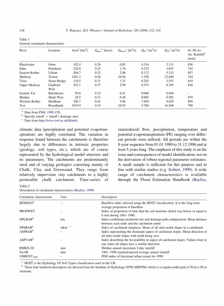
Table 1

General catchment characteristics

River Location Areaa [km2] Qspecb [m/yr] Qmean

c [m3/s] Q95c [m3/s] Q10

c [m3/s] 61–90 Av.

An. Rainfall2

[mm]

Blackwater Ower 102.4 0.26 0.85 0.154 2.131 836

Eden Penshurst 224.8 0.25 1.76 0.232 3.853 742

Eastern Rother Udiam 204.7 0.32 2.08 0.172 5.312 857

Medway Teston 1261.3 0.26 10.56 1.526 23.840 744

Teise Stone Bridge 134.5 0.31 1.31 0.202 2.553 810

Upper Medway Chafford

Weir

252.1 0.37 2.99 0.533 6.395 830

Eastern Yar Burnthouse 59.6 0.22 0.41 0.040 0.846 -

Medina Shide Weir 28.5 0.31 0.28 0.082 0.502 839

Western Rother Hardham 360.7 0.43 4.96 1.694 9.829 899

Test Broadlands 1035.9 0.33 10.93 5.780 16.560 790

a Data from FEH, 1999, CD.b Specific runoff Z runoff / drainage area.c Data from http://www.nwl.ac.uk/ih/nrfa.

T. Wagener, H.S. Wheater / Journal of Hydrology 320 (2006) 132–154136

climatic data (precipitation and potential evapotran-

spiration) are highly correlated. The variation in

response found between the catchments is therefore

largely due to differences in intrinsic properties

(geology, soil types, etc.), which are of course

represented by the hydrological model structure and

its parameters. The catchments are predominantly

rural and of varying geologies consisting mainly of

Chalk, Clay and Greensand. They range from

relatively impervious clay catchments to a highly

permeable chalk catchment. Time-series of

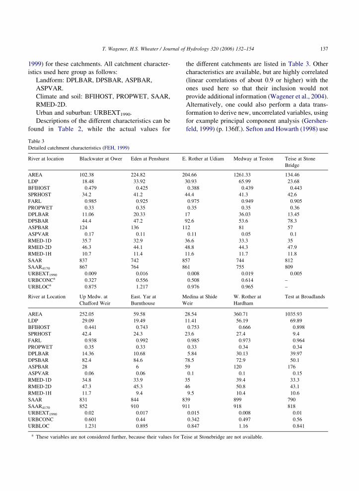
Table 2

Description of catchment characteristics (Bayliss, 1999)

Catchment characteristic Unit Description

BFIHOSTa – Baseflow in

average pro

PROPWET – Index of pro

6 mm durin

DPLBARb km Index comb

between eac

DPSBARb mkmK1 Index of cat

ASPBARb – Index repres

all inter-nod

ASPVARb – Index descri

one when al

RMED-2D mm Median ann

SAAR mm 1961–1990

URBEXT1990 – FEH index o

a HOST is the Hydrology Of Soil Types classification used in the UK.b These four landform descriptors are derived from the Institute of Hydr

elements.

(naturalized) flow, precipitation, temperature and

potential evapotranspiration (PE) ranging over differ-

ent periods were utilized. All periods are within the

8-year sequence from 01.01.1989 to 31.12.1996 and at

least 5 years long. The emphasis of this study is on the

issue and consequences of model identification, not on

the derivation of robust regional parameter estimates.

A small sample is sufficient for this purpose and in

line with similar studies (e.g. Seibert, 1999). A wide

range of catchment characteristics is available

through the Flood Estimation Handbook (Bayliss,

dex derived using the HOST classification. It is the long-term

portion of baseflow

portion of time that the soil moisture deficit was below or equal to

g 1961–1990

ining catchment size and drainage path configuration. Mean distance

h node and the catchment outlet

chment steepness. Mean of all inter-nodal slopes in a catchment

enting the dominant aspect of catchment slopes. Mean direction of

al slopes with north being zero

bing the invariability in aspect of catchment slopes. Values close to

l slopes face a similar direction

ual maximum 2-day rainfall

standard-period average annual rainfall

f fractional urban extent for 1990

ology DTM (IHDTM) which is a regular nodal grid of 50 m!50 m

T. Wagener, H.S. Wheater / Journal of Hydrology 320 (2006) 132–154 137

1999) for these catchments. All catchment character-

istics used here group as follows:

Landform: DPLBAR, DPSBAR, ASPBAR,

ASPVAR.

Climate and soil: BFIHOST, PROPWET, SAAR,

RMED-2D.

Urban and suburban: URBEXT1990.

Descriptions of the different characteristics can be

found in Table 2, while the actual values for

Table 3

Detailed catchment characteristics (FEH, 1999)

River at location Blackwater at Ower Eden at Penshurst E

AREA 102.38 224.82 2

LDP 18.48 33.92

BFIHOST 0.479 0.425

SPRHOST 34.2 41.2

FARL 0.985 0.925

PROPWET 0.33 0.35

DPLBAR 11.06 20.33

DPSBAR 44.4 47.2

ASPBAR 124 136 1

ASPVAR 0.17 0.11

RMED-1D 35.7 32.9

RMED-2D 46.3 44.1

RMED-1H 10.7 11.4

SAAR 837 742 8

SAAR4170 867 764 8

URBEXT1990 0.009 0.016

URBCONCa 0.327 0.556

URBLOCa 0.875 1.217

River at Location Up Medw. at

Chafford Weir

East. Yar at

Burnthouse

M

W

AREA 252.05 59.58

LDP 29.09 19.49

BFIHOST 0.441 0.743

SPRHOST 42.4 24.3

FARL 0.938 0.992

PROPWET 0.35 0.33

DPLBAR 14.36 10.68

DPSBAR 82.4 84.6

ASPBAR 28 6

ASPVAR 0.06 0.06

RMED-1D 34.8 33.9

RMED-2D 47.3 45.3

RMED-1H 11.7 9.4

SAAR 831 844 8

SAAR4170 852 910 9

URBEXT1990 0.02 0.017

URBCONC 0.601 0.44

URBLOC 1.231 0.895

a These variables are not considered further, because their values for Te

the different catchments are listed in Table 3. Other

characteristics are available, but are highly correlated

(linear correlations of about 0.9 or higher) with the

ones used here so that their inclusion would not

provide additional information (Wagener et al., 2004).

Alternatively, one could also perform a data trans-

formation to derive new, uncorrelated variables, using

for example principal component analysis (Gershen-

feld, 1999) (p. 136ff.). Sefton and Howarth (1998) use

. Rother at Udiam Medway at Teston Teise at Stone

Bridge

04.66 1261.33 134.46

30.93 65.99 23.68

0.388 0.439 0.443

44.4 41.3 42.6

0.975 0.949 0.905

0.35 0.35 0.36

17 36.03 13.45

92.6 53.6 78.3

12 81 57

0.11 0.05 0.1

36.6 33.3 35

48.8 44.3 47.9

11.6 11.7 11.8

57 744 812

61 755 809

0.008 0.019 0.005

0.508 0.614 –

0.976 0.965 –

edina at Shide

eir

W. Rother at

Hardham

Test at Broadlands

28.54 360.71 1035.93

11.41 56.19 69.89

0.753 0.666 0.898

23.6 27.4 9.4

0.985 0.973 0.964

0.33 0.34 0.34

5.84 30.13 39.97

78.5 72.9 50.1

59 120 176

0.1 0.1 0.15

35 39.4 33.3

46 50.8 43.1

9.5 10.4 10.6

39 899 790

11 918 818

0.015 0.008 0.01

0.342 0.497 0.56

0.847 1.16 0.841

ise at Stonebridge are not available.

T. Wagener, H.S. Wheater / Journal of Hydrology 320 (2006) 132–154138

principal components to derive variables that they call

topography and soils/geology for regional analysis

from an initial set of catchment characteristics.

However, the newly derived variables reduce the

ease with which regional relationships can be

interpreted. This approach is therefore not considered

here.

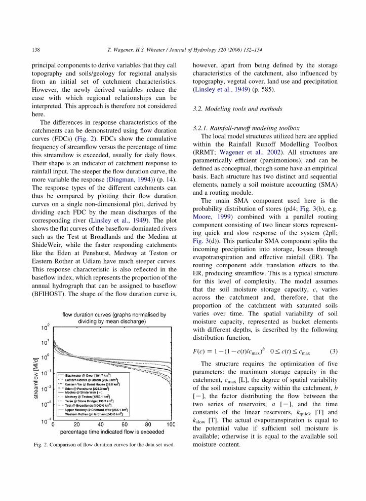
The differences in response characteristics of the

catchments can be demonstrated using flow duration

curves (FDCs) (Fig. 2). FDCs show the cumulative

frequency of streamflow versus the percentage of time

this streamflow is exceeded, usually for daily flows.

Their shape is an indicator of catchment response to

rainfall input. The steeper the flow duration curve, the

more variable the response (Dingman, 1994)) (p. 14).

The response types of the different catchments can

thus be compared by plotting their flow duration

curves on a single non-dimensional plot, derived by

dividing each FDC by the mean discharges of the

corresponding river (Linsley et al., 1949). The plot

shows the flat curves of the baseflow-dominated rivers

such as the Test at Broadlands and the Medina at

ShideWeir, while the faster responding catchments

like the Eden at Penshurst, Medway at Teston or

Eastern Rother at Udiam have much steeper curves.

This response characteristic is also reflected in the

baseflow index, which represents the proportion of the

annual hydrograph that can be assigned to baseflow

(BFIHOST). The shape of the flow duration curve is,

Fig. 2. Comparison of flow duration curves for the data set used.

however, apart from being defined by the storage

characteristics of the catchment, also influenced by

topography, vegetal cover, land use and precipitation

(Linsley et al., 1949) (p. 585).

3.2. Modeling tools and methods

3.2.1. Rainfall-runoff modeling toolbox

The local model structures utilized here are applied

within the Rainfall Runoff Modelling Toolbox

(RRMT; Wagener et al., 2002). All structures are

parametrically efficient (parsimonious), and can be

defined as conceptual, though some have an empirical

basis. Each structure has two distinct and sequential

elements, namely a soil moisture accounting (SMA)

and a routing module.

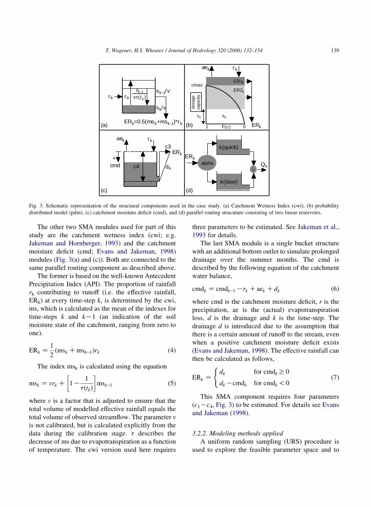
The main SMA component used here is the

probability distribution of stores (pd4; Fig. 3(b), e.g.

Moore, 1999) combined with a parallel routing

component consisting of two linear stores represent-

ing quick and slow response of the system (2pll;

Fig. 3(d)). This particular SMA component splits the

incoming precipitation into storage, losses through

evapotranspiration and effective rainfall (ER). The

routing component adds translation effects to the

ER, producing streamflow. This is a typical structure

for this level of complexity. The model assumes

that the soil moisture storage capacity, c, varies

across the catchment and, therefore, that the

proportion of the catchment with saturated soils

varies over time. The spatial variability of soil

moisture capacity, represented as bucket elements

with different depths, is described by the following

distribution function,

FðcÞ Z 1Kð1KcðtÞ=cmaxÞb 0%cðtÞ%cmax (3)

The structure requires the optimization of five

parameters: the maximum storage capacity in the

catchment, cmax [L], the degree of spatial variability

of the soil moisture capacity within the catchment, b

[K], the factor distributing the flow between the

two series of reservoirs, a [K], and the time

constants of the linear reservoirs, kquick [T] and

kslow [T]. The actual evapotranspiration is equal to

the potential value if sufficient soil moisture is

available; otherwise it is equal to the available soil

moisture content.

k(quick)

k(slow)

(a) (b)

(c) (d)

cmd+

c3

c4

rk rk

ERk=0.5(msk+msk-1)*rk

dk

rkaek

)( k

k

tvst

1- sk-1/v

sk/v

ER1k

stor

age

capa

city

F(c)

sk

cmaxER2k

1 0

ck

rkaek

ERk

alphaERk

+

ERk

Qk

Fig. 3. Schematic representation of the structural components used in the case study. (a) Catchment Wetness Index (cwi), (b) probability

distributed model (pdm), (c) catchment moisture deficit (cmd), and (d) parallel routing strucuture consisting of two linear reservoirs.

T. Wagener, H.S. Wheater / Journal of Hydrology 320 (2006) 132–154 139

The other two SMA modules used for part of this

study are the catchment wetness index (cwi; e.g.

Jakeman and Hornberger, 1993) and the catchment

moisture deficit (cmd; Evans and Jakeman, 1998)

modules (Fig. 3(a) and (c)). Both are connected to the

same parallel routing component as described above.

The former is based on the well-known Antecedent

Precipitation Index (API). The proportion of rainfall

rk contributing to runoff (i.e. the effective rainfall,

ERk) at every time-step k, is determined by the cwi,

ms, which is calculated as the mean of the indexes for

time-steps k and kK1 (an indication of the soil

moisture state of the catchment, ranging from zero to

one).

ERk Z1

2ðmsk CmskK1Þrk (4)

The index msk is calculated using the equation

msk Z vrk C 1K1

tðtkÞ

� �mskK1 (5)

where v is a factor that is adjusted to ensure that the

total volume of modelled effective rainfall equals the

total volume of observed streamflow. The parameter v

is not calibrated, but is calculated explicitly from the

data during the calibration stage. t describes the

decrease of ms due to evapotranspiration as a function

of temperature. The cwi version used here requires

three parameters to be estimated. See Jakeman et al.,

1993 for details.

The last SMA module is a single bucket structure

with an additional bottom outlet to simulate prolonged

drainage over the summer months. The cmd is

described by the following equation of the catchment

water balance,

cmdk Z cmdkK1Krk Caek Cdk (6)

where cmd is the catchment moisture deficit, r is the

precipitation, ae is the (actual) evapotranspiration

loss, d is the drainage and k is the time-step. The

drainage d is introduced due to the assumption that

there is a certain amount of runoff to the stream, even

when a positive catchment moisture deficit exists

(Evans and Jakeman, 1998). The effective rainfall can

then be calculated as follows,

ERk Zdk for cmdk R0

dk Kcmdk for cmdk !0

((7)

This SMA component requires four parameters

(c1Kc4, Fig. 3) to be estimated. For details see Evans

and Jakeman (1998).

3.2.2. Modeling methods applied

A uniform random sampling (URS) procedure is

used to explore the feasible parameter space and to

T. Wagener, H.S. Wheater / Journal of Hydrology 320 (2006) 132–154140

allow for an estimate of the uncertainty in the para-

meter estimates. In this case, the parameters are

assumed independent from each other and the only

prior information used is reasonable lower and upper

boundary values. 10,000 parameter sets are randomly

sampled for each case. Initial conditions (model mois-

ture states) are calibrated instead of using a warm-up

period to ensure that the results are independent of the

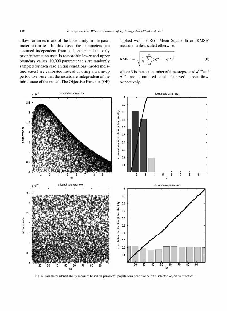
initial state of the model. The Objective Function (OF)

Fig. 4. Parameter identifiability measure based on parameter p

applied was the Root Mean Square Error (RMSE)

measure, unless stated otherwise.

RMSE Z

ffiffiffiffiffiffiffiffiffiffiffiffiffiffiffiffiffiffiffiffiffiffiffiffiffiffiffiffiffiffiffiffiffiffiffiffiffiffiffi1

N

XN

tZ1

ðqsimt Kqobs

t Þ2

vuut (8)

where N is the total number of time steps t, and qsim and

qobs are simulated and observed streamflow,

respectively.

opulations conditioned on a selected objective function.

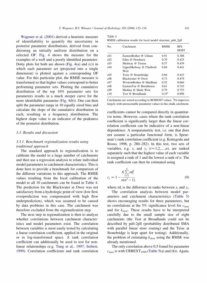
Table 4

RMSE calibration results for local model structure, pd4_2pll

No. Catchment RMSE BFI-

HOST

c01 EasternRother @ Udiam 0.91 0.388

c02 Eden @ Penshurst 0.70 0.425

c03 Medway @ Teston 0.57 0.439

c04 UpperMedway @ Chafford-

Weir

0.84 0.441

c05 Teise @ Stonebridge 0.66 0.443

c06 Blackwater @ Ower 0.73 0.479

c07 WesternRother @ Hardham 0.52 0.666

c08 EasternYar @ Burnthouse 0.61 0.743

c09 Medina @ Shide Weir 0.79 0.753

c10 Test @ Broadlands 0.191 0.898

Catchments are sorted according to BFIHOST values. 1Fit improves

largely with unreasonable parameter values in this chalk catchment.

T. Wagener, H.S. Wheater / Journal of Hydrology 320 (2006) 132–154 141

Wagener et al. (2001) derived a heuristic measure

of identifiability to quantify the uncertainty in

posterior parameter distributions, derived from con-

ditioning an initially uniform distribution on a

selected OF. Fig. 4 shows the measure for the

examples of a well and a poorly identified parameter.

Dotty plots for both are shown (Fig. 4(a) and (c)) in

which each parameter set (projected into a single

dimension) is plotted against a corresponding OF

value. For this particular plot, the RMSE measure is

transformed so that higher values correspond to better

performing parameter sets. Plotting the cumulative

distribution of the top 10% parameter sets for

parameters results in a much steeper curve for the

more identifiable parameter (Fig. 4(b)). One can then

split the parameter range in 10 equally sized bins and

calculate the slope of the cumulative distribution in

each, resulting in a frequency distribution. The

highest slope value is an indicator of the peakiness

of the posterior distribution.

3.3. Results and discussion

3.3.1. Benchmark regionalization results using

traditional approach

The standard approach to regionalization is to

calibrate the model to a large number of catchments

and then use a regression analysis to relate individual

model parameters to catchment characteristics. This is

done here to provide a benchmark for comparison of

the different variations to this approach. The RMSE

values resulting from the local calibration of the

model to all 10 catchments can be found in Table 4.

The prediction for the Blackwater at Ower was not

satisfactory from a hydrologic point of view (low flow

overprediction was compensated with high flow

underprediction), which was assumed to be caused

by data problems in this case. The catchment was

therefore excluded from the regionalization step.

The next step in regionalization is then to analyze

whether correlations between catchment character-

istics and model parameters exist. The correlation

between variables is most easily tested by calculating

a linear correlation coefficient, applied in the original

or in log-transformed space. A rank correlation

coefficient can additionally be used to test for non-

linear relationships (e.g. Tung et al., 1997; Seibert,

1999). Correlation coefficients and rank correlation

coefficients cannot be compared directly in quantitat-

ive terms. However, cases where the rank correlation

coefficient is significantly larger than the linear cor-

relation coefficient can be indicative of a non-linear

dependence. A nonparametric test, i.e. one that does

not assume a particular functional form, is Spear-

man’s rank correlation coefficient (e.g. Kottegoda and

Rosso, 1998, p. 280–282). In this test, two sets of

variables, e.g. xi and yi (iZ1,2,.,n), are ranked

separately such that the highest value of each variable

is assigned a rank of 1 and the lowest a rank of n. The

rank coefficient can then be estimated using

rs Z 1K

6Pn

iZ1

rd2i

nðn2 K1Þ(9)

where rdi is the difference in ranks between xi and yi.

The correlation analysis between model par-

ameters and catchment characteristics (Table 5)

shows encouraging results for three parameters, but

no correlations at the 5% significance level for cmax

and for kslow. These results have to be interpreted

carefully due to the small sample size of eight

catchments (the Test at Broadlands could not be

described by pd4-2pll (probability distributed SMA

with parallel linear store routing) and the Teise at

Stonebridge is kept apart for testing). Additionally,

the problem of estimating kslow using the RMSE was

already mentioned.

The only correlation above 0.5 found for parameter

cmax is with URBEXT1990 (Table 5(a) and (b)). Again,

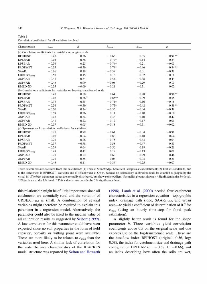
Table 5

Correlation coefficients for all variables involved

Characteristic cmax B kquick kslow a

(a) Correlation coefficients for variables on original scale

BFIHOST 0.43 0.56 K0.66 0.35 K0.91**

DPLBAR K0.04 K0.58 0.72* K0.14 0.34

DPSBAR K0.36 0.23 K0.74* 0.21 K0.03

PROPWET K0.35 K0.59 0.74* K0.46 0.84**

SAAR K0.16 0.18 K0.59 0.01 K0.31

URBEXT1990 0.57 0.15 0.13 0.02 K0.18

ASPBAR K0.41 K0.34 0.54 K0.38 0.44

ASPVAR K0.43 0.09 K0.05 K0.29 0.13

RMED-2D K0.35 K0.09 K0.21 K0.31 0.02

(b) Correlation coefficients for variables on log–log-transformed scale

BFIHOST 0.47 0.58 K0.64 0.28 K0.96**

DPLBAR K0.03 K0.66f 0.85** K0.09 0.55

DPSBAR K0.38 0.45 K0.71* 0.10 K0.18

PROPWET K0.34 K0.59 0.75* K0.42 0.89**

SAAR K0.20 0.34 K0.56 K0.04 K0.38

URBEXT1990 0.59 0.26 0.11 K0.10 K0.10

ASPBAR K0.43 K0.34 0.38 K0.40 0.42

ASPVAR K0.41 K0.22 K0.12 K0.17 0.01

RMED-2D K0.37 0.05 K0.18 K0.31 K0.02

(c) Spearman rank correlation coefficients for variables

BFIHOST 0.21 0.79 K0.61 K0.04 K0.96

DPLBAR K0.07 K0.64 0.86 K0.18 0.64

DPSBAR K0.21 0.28 K0.75 0.43 K0.04

PROPWET K0.37 K0.78 0.58 K0.47 0.83

SAAR K0.29 0.04 K0.50 0.18 K0.21

URBEXT1990 0.49 0.42 0.19 K0.13 0.01

ASPBAR K0.21 K0.82 0.68 K0.29 0.46

ASPVAR K0.21 K0.55 0.06 K0.03 0.21

RMED-2D K0.43 0.11 K0.36 K0.25 K0.07

Three catchments are excluded from this calculation: (1) Teise at Stonebridge, because it is kept as a test catchment; (2) Test at Broadlands, due

to the differences in BFIHOST (see text); and (3) Blackwater at Ower, because no satisfactory calibration could be established judged by the

visual fit. (The best parameter values are normally distributed, but show some outliers. Normality plot not shown.). *Significant at the 5% level.

**Significant at the 1% level. fThis value is just outside the 5% significance level.

T. Wagener, H.S. Wheater / Journal of Hydrology 320 (2006) 132–154142

this relationship might be of little importance since all

catchments are essentially rural and the variation of

URBEXT1990 is small. A combination of several

variables might therefore be required to explain this

parameter in a regression model. Alternatively, the

parameter could also be fixed to the median value of

all calibration results as suggested by Seibert (1999).

A low correlation for this parameter could have been

expected since no soil properties in the form of field

capacity, porosity or wilting point were available.

These are more likely to be related to cmax than the

variables used here. A similar lack of correlation for

the water balance characteristics of the IHACRES

model structure was reported by Sefton and Howarth

(1998). Lamb et al. (2000) needed four catchment

characteristics in a regression equation—topographic

index, drainage path slope, SAAR61–90, and urban

area—to yield a coefficient of determination of 0.7 for

cmax (using an hourly time-step for flood peak

estimation).

A slightly better result is found for the shape

parameter b. Three variables yield correlation

coefficients above 0.5 on the original scale and one

exceeds 0.6 on the log-transformed scale. These are

the baseflow index BFIHOST (original: 0.56, log:

0.58), the index for catchment size and drainage path

configuration DPLBAR (o.: K0.58, l.: K0.66), and

an index describing how often the soils are wet,

T. Wagener, H.S. Wheater / Journal of Hydrology 320 (2006) 132–154 143

PROPWET (o.: K0.60, l.: K0.59). However, only the

correlation to DPLBAR (on log-scale) is significant at

the 5% level. The variable PROPWET is unlikely to

be very useful in a regression since it only takes four

different values within the available data-set (0.33,

0.34, 0.35 and 0.36). A value of zero for b is equal to a

constant storage capacity over the catchment, while a

value of 1 yields a uniform distribution of storage

capacities. The results suggest higher b values for

catchments with a larger contribution of baseflow,

smaller catchment area and drier soils. The shape of

the storage distribution function b is the only

parameter for which the Spearman rank correlation

coefficient gives considerably higher values than the

linear correlation coefficients on normal or log-

transformed scale (Table 5(c)). The highest rank

correlation values are found with the variables

ASPBAR (K0.82), BFIHOST (0.79) and PROPWET

(K0.78). There is also a relatively high value with

DPLBAR (K0.64). The fact that the (non-parametric)

rank correlations are higher than those assuming a

linear relationship is indicative of a possible non-

linear relationship. The variable ASPBAR describes

the mean aspect of the catchment. It is calculated as an

average from the outflow direction (bearing) of each

nodal point on the IHDTM within a catchment. It is

therefore an indicator of the dominant aspect of

catchment slopes. Its values increase clockwise from

zero to 3608, starting from the north. A negative rank

correlation suggests that a south-easterly bearing is

related to a lower b value.

The parameter kquick is correlated with a number of

characteristics, BFIHOST (o.: K0.66, l.: K0.64),

DPLBAR (o.: 0.72, l.: 0.85), the mean drainage path

slope index DPSBAR (o.: K0.74, l.: K0.71),

PROPWET (o.: 0.74, l.: 0.75) and average annual

rainfall over a selected period SAAR (o.: K0.59, l.:

K0.56). The largest correlation is found with

DPLBAR (on log-scale). The variable DPLBAR is

the mean drainage path distance of all nodes of the

IHDTM to the catchment outlet. The result suggests

that larger and more elongated catchments drain more

slowly. On the contrary, steeper catchments produce

smaller time constants, and the mean drainage path

slope (DPSBAR) is higher. Again, the correlation

with PROPWET is probably of little explanatory

value. As noted above, the values of the catchments

used only vary between 0.33 and 0.36, while the UK

wide variation is between 0.20 and 0.85. Sefton and

Howarth (1998) related the quick response time

constant (within the IHACRES model structure) to

catchment size and stream-frequency, but found no

improvement when including channel slope. In the

study by Lamb et al. (2000), this parameter showed

the highest correlation of the four PDM parameters

tested (the fast/slow split was fixed). They derived it

from BFIHOST, stream network centroid, MORECS

residual soil moisture and suburban area.

The slow flow time constant kslow does not show

any significant (5% level) correlation with any of the

available catchment characteristics. This is not

unexpected since this is the least identifiable

parameter. The problem of identifying this parameter

(and other parameters related to the low flow periods

for that matter) using an OF based on the complete

hydrograph is one of the main reasons why

segmentation schemes were introduced (e.g. Dunne,

1999; Boyle et al., 2000; Wagener et al., 2001). It

seems quite unlikely that a parameter such as the slow

flow time constant can be regionalized based on a

calibration using an OF that emphasizes the fit to high

flow, such as the RMSE. Similar results have been

reported by other researchers. Lamb et al. (2000)

derive a regional equation to estimate this parameter

from BFIHOST, soil porosity and underlying geology.

However, the coefficient of determination produced

by their model is 0.6 and thus the lowest of their four

regionalized model parameters. Their result is similar

to the one by Sefton and Howarth (1998) who relate a

slow flow time constant to different soil variables. The

correlation coefficient between regionalized and

locally calibrated values was only 0.37, however.

The fraction of effective rainfall that contributes to

the quick response, a, is highly correlated to two

catchment characteristics, the baseflow index BFI-

HOST and PROPWET. The first correlation (on

original scale) is negative (o.: K0.91; l.: K0.96),

while the second one is positive (o.: 0.84; l.: 0.89).

Both are significant at the 1% level. The first

correlation is expected, while the second indicates

that a wet catchment, probably containing more

saturated and therefore contributing areas, produces

a high percentage of quick response. Sefton and

Howarth (1998) found that the contribution to slow

response (1Ka) was highly correlated to the

percentage of aquifer in a catchment (0.77), a variable

T. Wagener, H.S. Wheater / Journal of Hydrology 320 (2006) 132–154144

not available here. This split parameter is sometimes

assumed to be directly equal to the standard

percentage runoff (SPRHOST) or BFIHOST, e.g.

Lamb et al. (1999) and Young (2002). SPRHOST is

highly correlated to BFIHOST as shown earlier

(K0.98). The result found here therefore suggests

that fixing this parameter a priori using BFIHOST can

be justifiable.

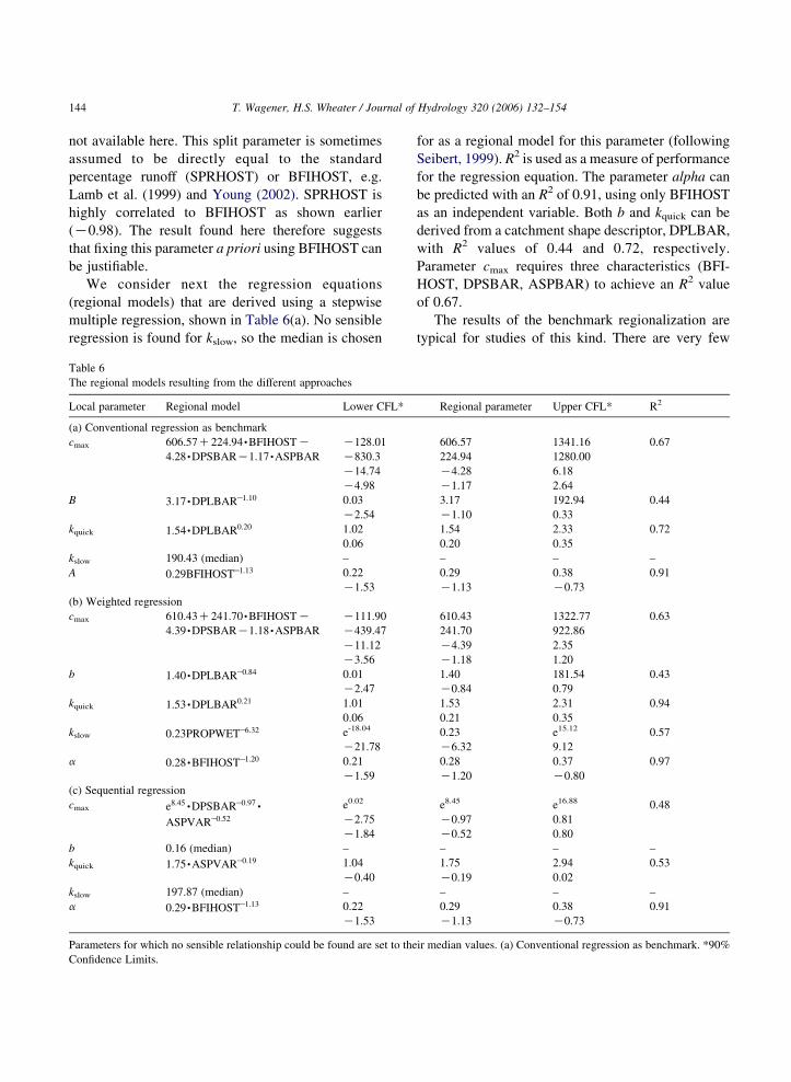
We consider next the regression equations

(regional models) that are derived using a stepwise

multiple regression, shown in Table 6(a). No sensible

regression is found for kslow, so the median is chosen

Table 6

The regional models resulting from the different approaches

Local parameter Regional model Lower CFL*

(a) Conventional regression as benchmark

cmax 606:57C224:94,BFIHOSTK

4:28,DPSBARK1:17,ASPBAR

K128.01

K830.3

K14.74

K4.98

B 3:17,DPLBARK1:10 0.03

K2.54

kquick 1:54,DPLBAR0:20 1.02

0.06

kslow 190.43 (median) –

A 0:29BFIHOSTK1:13 0.22

K1.53

(b) Weighted regression

cmax 610:43C241:70,BFIHOSTK4:39,DPSBARK1:18,ASPBAR

K111.90

K439.47

K11.12

K3.56

b 1:40,DPLBARK0:84 0.01

K2.47

kquick 1:53,DPLBAR0:21 1.01

0.06

kslow 0:23PROPWETK6:32 e-18.04

K21.78

a 0:28,BFIHOSTK1:20 0.21

K1.59

(c) Sequential regression

cmax e8:45,DPSBARK0:97,

ASPVARK0:52

e0.02

K2.75

K1.84

b 0.16 (median) –

kquick 1:75,ASPVARK0:19 1.04

K0.40

kslow 197.87 (median) –

a 0:29,BFIHOSTK1:13 0.22

K1.53

Parameters for which no sensible relationship could be found are set to the

Confidence Limits.

for as a regional model for this parameter (following

Seibert, 1999). R2 is used as a measure of performance

for the regression equation. The parameter alpha can

be predicted with an R2 of 0.91, using only BFIHOST

as an independent variable. Both b and kquick can be

derived from a catchment shape descriptor, DPLBAR,

with R2 values of 0.44 and 0.72, respectively.

Parameter cmax requires three characteristics (BFI-

HOST, DPSBAR, ASPBAR) to achieve an R2 value

of 0.67.

The results of the benchmark regionalization are

typical for studies of this kind. There are very few

Regional parameter Upper CFL* R2

606.57 1341.16 0.67

224.94 1280.00

K4.28 6.18

K1.17 2.64

3.17 192.94 0.44

K1.10 0.33

1.54 2.33 0.72

0.20 0.35

– – –

0.29 0.38 0.91

K1.13 K0.73

610.43 1322.77 0.63

241.70 922.86

K4.39 2.35

K1.18 1.20

1.40 181.54 0.43

K0.84 0.79

1.53 2.31 0.94

0.21 0.35

0.23 e15.12 0.57

K6.32 9.12

0.28 0.37 0.97

K1.20 K0.80

e8.45 e16.88 0.48

K0.97 0.81

K0.52 0.80

– – –

1.75 2.94 0.53

K0.19 0.02

– – –

0.29 0.38 0.91

K1.13 K0.73

ir median values. (a) Conventional regression as benchmark. *90%

T. Wagener, H.S. Wheater / Journal of Hydrology 320 (2006) 132–154 145

parameters for which some robust correlation of

significance can be found. The remaining ones show

little or no correlation. An in-depth analysis to

investigate the possible reasons for this problem is

provided in the following sections, including the

testing of variations on the traditional approach.

3.3.2. Does a model component, implemented

in different model structures, yield the same

optimal parameters?

A large variety of model structures is applied in

hydrological research and practice. However, the

number of model components (e.g. linear reservoir,

overflow bucket, etc.) from which these structures are

composed is relatively small (Wagener et al., 2002).

Different model structures therefore usually have

some components in common. One would expect that

Fig. 5. Comparison of kquick [d], kslow [d] and a [K] values for the pd4-2pll

with respect to the RMSE criterion. Catchments are sorted from left to rig

the same optimal model parameters would be found

for these components if they have the same functional

purpose within the different model structures, i.e. if

they represent identical processes. Additional model

structures, to the above analyzed pd4, all a priori

equally suitable to represent the hydrological system

under study, are applied to all catchments to test this

assumption. Research results by others (Beven and

Franks, 1999; Kokkonen and Jakeman, 2001) suggest

that identical components (and therefore parameters)

used within different model structures can have

different optimum parameters due to interaction

between the different model components. This is

tested here by applying two further model structures.

The SMA component is represented by an empirical

(cwi) and an additional conceptual model structure

(cmd) respectively, using routing components

, cwi-2pll and cmd_2pll model structures. Values shown are optimal

ht with increasing Baseflow index (BFIHOST).

Fig. 6. Plot of identifiability measure values (based on the RMSE)

versus catchments (c1–c10) for different parameters. Catchments

are sorted from left to right with increasing Baseflow index

(BFIHOST).

T. Wagener, H.S. Wheater / Journal of Hydrology 320 (2006) 132–154146

identical to the linear parallel structure used in the

model structure described above. The resulting

routing parameters are compared to see whether we

could corroborate or refute the above mentioned

results. The metric and the second parametric model

structures are applied to all catchments using the same

URS approach (10,000 samples) as before and the best

kquick, kslow and a parameters for all structures are

selected based on the RMSE criterion. The variation

in optimum values is shown in Fig. 5. It can be seen

that with respect to kquick, all model structures show a

relatively high degree of similarity in optimum

values. Generally this parameter seems to show little

dependency on the soil moisture accounting (SMA)

module, and experience has shown that kquick is

usually well identified (e.g. Wagener et al., 2001)

However, there is a slight tendency for cwi to produce

higher values. The result for kslow shows that it is

difficult to identify this parameter using the overall

RMSE as OF. The optimum values vary widely and

there appears to be little structure. This result is not

sufficiently reliable to draw any conclusions. The a

values for the cwi module are consistently the lowest

for all catchments, i.e. a smaller contribution to

quickflow and therefore a larger baseflow component.

They also show an even more pronounced trend of a

decrease with increasing BFIHOST values than the

estimates for the other two SMA modules. This

supports the result of Kokkonen and Jakeman (2001)

with respect to this parameter. They also found that

using a metric SMA module resulted in a smaller

contribution to quickflow.

This result suggests that a parameter estimation

procedure is required that considers the functional

purpose of the model component within the overall

structure. If the parameters representing the com-

ponent cannot be separated out during calibration,

then it is likely that the interaction with the other

model components will distort the parameter estimate

and limit the chances for success in finding

correlations with catchment characteristics.

3.3.3. What is the relationship between local

parameter identifiability and catchment

characteristics?

A model structure that is a sensible representation

of the hydrologic system under study should exhibit

identifiable parameters if a suitable strategy is applied

for parameter estimation (mainly a suitable OF is

defined) and if sufficiently informative data is

available. The identifiability of the parameters is

therefore an indicator of the suitability of the model

structure, within the limits of the information content

of the data. It was already mentioned that BFIHOST

(the baseflow index, representing underlying geology)

is the main characteristic that defines the response

behavior of the 10 catchments used in this study. A

way to quantify the identifiability (and therefore the

uncertainty) of model parameters has been introduced

above in the form of an identifiability measure (Fig. 4).

Fig. 6 shows the 10 catchments sorted by increasing

baseflow index (BFIHOST) from left to right versus the

identifiability of the model parameters of the pdm

SMA component connected to the parallel linear

routing component.

The maximum storage capacity cmax and the slow

flow time constant kslow do not show any significant

T. Wagener, H.S. Wheater / Journal of Hydrology 320 (2006) 132–154 147

relationship between baseflow index and identifia-

bility. In case of kslow this is likely to be due to the fact

that the RMSE, which emphases peak flows, was

selected. The remaining three parameters on the other

hand show a certain trend. The parameter describing

the shape of the Pareto distribution of storage

elements, b, is clearly more identifiable for the

catchments with a medium baseflow index and

mixed geology. This parameter defines the variability

of runoff production within the catchment and seems

more identifiable when the catchments are more

heterogeneous. The quick flow time constant kquick is

more identifiable for the clay dominated, quick

responding, catchments. Here, the difference between

quick and slow drainage slopes is very pronounced.

The parameter that splits the effective rainfall into

quick and slow response is most identifiable in the

catchments that are either clearly clay (small baseflow

index) or clearly chalk dominated (high baseflow

index). Here, the model tends to require that either

most of the effective rainfall is feeding the quick or

the slow response.

The fact that the parameters of a model, which is

commonly assumed to equally represent all catch-

ments included in this study, vary in identifiability is

important for the use of this result in a subsequent

regionalization step. Each optimal parameter will be

one data point when the correlation between par-

ameters and catchment characteristics is calculated. It

does not seem to be sensible to give the same weight to

identifiable parameters than to parameters that are

unidentifiable and therefore highly uncertain. Wagener

et al. (2004) show that this uncertainty can be

considered during regionalization if a weighted

regression procedure is applied (Appendix A). The

identifiability measures can be used as weights in this

methodology. The results of the weighted regression

are summarized in Table 6(b). In general, the

catchment characteristics identified as significant in

the regional models remain identical to those of the

benchmark regression. The main difference is that it is

now possible to derive a regional model for kslow,

though with low predictive power (R2Z0.57) and with

very wide uncertainty bounds on the regression para-

meters. Additionally, the uncertainty for the regression

parameters for cmax reduces. The expected values for

the regression parameters, and therefore the regiona-

lized parameters, remain almost identical though.

A straightforward way to propagate this uncer-

tainty into the predictions in the ungauged catchment

is to calculate the standard uncertainty on the

regression parameters (assuming Gaussian errors).

This will yield a reasonable estimate if the regression

residuals are close to normal (Kottegoda and Rosso,

1997). This will be the case if the variables used in the

regression follow normal distributions.

One can then randomly sample from ‘uncertain’

regional regression (for example based on a uniform

distribution) and thus produce an ensemble of

predictions for the ungauged catchment (Wagener

et al., 2004).

3.3.4. How is the uniqueness of catchments reflected

in regionalization?

Beven (2000) suggests that the uniqueness of the

response behavior of individual catchments might be

the main reason for the failure of earlier regionaliza-

tion attempts. A behavior that is unique and (at least

currently) unexplainable is a problem often encoun-

tered in regionalization studies. It usually shows in the

form of outliers when correlations between catchment

characteristics and model parameters are calculated.

A variety of regionalization studies in the literature

shows scatter plots in which one, or very few,

catchments behave very differently from the general

trend (e.g. Seibert, 1999). The same was found in this

study. Fig. 7 shows scatter plots between catchment

characteristics and some of the model parameters. The

bottom right plot of Fig. 7 shows the quickflow time

constant, kquick, plotted against DPSBAR, the index of

catchment steepness. However, one of the catchments

clearly exhibits a unique behavior that is not captured

by this catchment characteristic and leads to an

unreasonable relationship. A sensible treatment, in

absence of any further information, would be the

exclusion of the outlier and instead acceptance that

the regression relationship will yield sensible results

in most cases, but might fail in some. The outlier has

to be investigated in more detail separately.

3.3.5. What is the effect of local model structural

uncertainty on the regionalization result?

Various researchers have shown that current model

structures are generally incapable of matching high-

and low-flow behavior of a catchment simultaneously

with a single parameter set (Gupta et al., 1998; Boyle

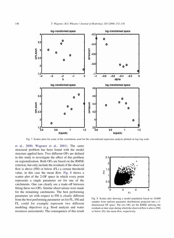
Fig. 7. Scatter plots for some of the correlations used for the conventional regression analysis plotted on log–log scale.

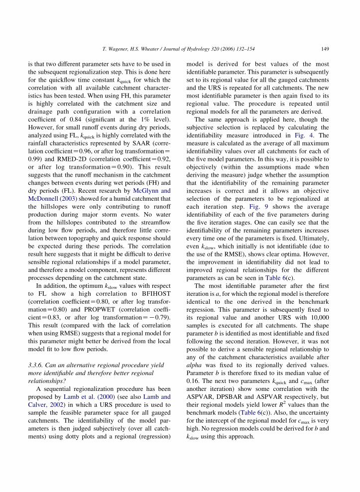
Fig. 8. Scatter plot showing a model population based on 10,000

samples from uniform parameter distributions projected into a 2-

dimensional OF space. The two OFs are the RMSE utilizing the

residuals at time steps during which the observed flow is above (FH)

or below (FL) the mean flow, respectively.

T. Wagener, H.S. Wheater / Journal of Hydrology 320 (2006) 132–154148

et al., 2000; Wagener et al., 2001). The same

structural problem has been found with the model

structure applied here. Two different OFs are defined

in this study to investigate the effect of this problem

on regionalization. Both OFs are based on the RMSE

criterion, but only include the residuals if the observed

flow is above (FH) or below (FL) a certain threshold

value, in this case the mean flow. Fig. 8 shows a

scatter plot of the 2-OF space in which every point

represents a single parameter set for one of the

catchments. One can clearly see a trade-off between

fitting these two OFs. Similar observations were made

for the remaining catchments. The best performing

parameter set with respect to FH is clearly different

from the best performing parameter set for FL. FH and

FL could for example represent two different

modeling objectives (e.g. flood analysis and water

resources assessment). The consequence of this result

T. Wagener, H.S. Wheater / Journal of Hydrology 320 (2006) 132–154 149

is that two different parameter sets have to be used in

the subsequent regionalization step. This is done here

for the quickflow time constant kquick for which the

correlation with all available catchment character-

istics has been tested. When using FH, this parameter

is highly correlated with the catchment size and

drainage path configuration with a correlation

coefficient of 0.84 (significant at the 1% level).

However, for small runoff events during dry periods,

analyzed using FL, kquick is highly correlated with the

rainfall characteristics represented by SAAR (corre-

lation coefficientZ0.96, or after log transformationZ0.99) and RMED-2D (correlation coefficientZ0.92,

or after log transformationZ0.90). This result

suggests that the runoff mechanism in the catchment

changes between events during wet periods (FH) and

dry periods (FL). Recent research by McGlynn and

McDonnell (2003) showed for a humid catchment that

the hillslopes were only contributing to runoff

production during major storm events. No water

from the hillslopes contributed to the streamflow

during low flow periods, and therefore little corre-

lation between topography and quick response should

be expected during these periods. The correlation

result here suggests that it might be difficult to derive

sensible regional relationships if a model parameter,

and therefore a model component, represents different

processes depending on the catchment state.

In addition, the optimum kslow values with respect

to FL show a high correlation to BFIHOST

(correlation coefficientZ0.80, or after log transfor-

mationZ0.80) and PROPWET (correlation coeffi-

cientZ0.83, or after log transformationZK0.79).

This result (compared with the lack of correlation

when using RMSE) suggests that a regional model for

this parameter might better be derived from the local

model fit to low flow periods.

3.3.6. Can an alternative regional procedure yield

more identifiable and therefore better regional

relationships?

A sequential regionalization procedure has been

proposed by Lamb et al. (2000) (see also Lamb and

Calver, 2002) in which a URS procedure is used to

sample the feasible parameter space for all gauged

catchments. The identifiability of the model par-

ameters is then judged subjectively (over all catch-

ments) using dotty plots and a regional (regression)

model is derived for best values of the most

identifiable parameter. This parameter is subsequently

set to its regional value for all the gauged catchments

and the URS is repeated for all catchments. The new

most identifiable parameter is then again fixed to its

regional value. The procedure is repeated until

regional models for all the parameters are derived.

The same approach is applied here, though the

subjective selection is replaced by calculating the

identifiability measure introduced in Fig. 4. The

measure is calculated as the average of all maximum

identifiability values over all catchments for each of

the five model parameters. In this way, it is possible to

objectively (within the assumptions made when

deriving the measure) judge whether the assumption

that the identifiability of the remaining parameter

increases is correct and it allows an objective

selection of the parameters to be regionalized at

each iteration step. Fig. 9 shows the average

identifiability of each of the five parameters during

the five iteration stages. One can easily see that the

identifiability of the remaining parameters increases

every time one of the parameters is fixed. Ultimately,

even kslow, which initially is not identifiable (due to

the use of the RMSE), shows clear optima. However,

the improvement in identifiability did not lead to

improved regional relationships for the different

parameters as can be seen in Table 6(c).

The most identifiable parameter after the first

iteration is a, for which the regional model is therefore

identical to the one derived in the benchmark

regression. This parameter is subsequently fixed to

its regional value and another URS with 10,000

samples is executed for all catchments. The shape

parameter b is identified as most identifiable and fixed

following the second iteration. However, it was not

possible to derive a sensible regional relationship to

any of the catchment characteristics available after

alpha was fixed to its regionally derived values.

Parameter b is therefore fixed to its median value of

0.16. The next two parameters kquick and cmax (after

another iteration) show some correlation with the

ASPVAR, DPSBAR and ASPVAR respectively, but

their regional models yield lower R2 values than the

benchmark models (Table 6(c)). Also, the uncertainty

for the intercept of the regional model for cmax is very

high. No regression models could be derived for b and

kslow using this approach.

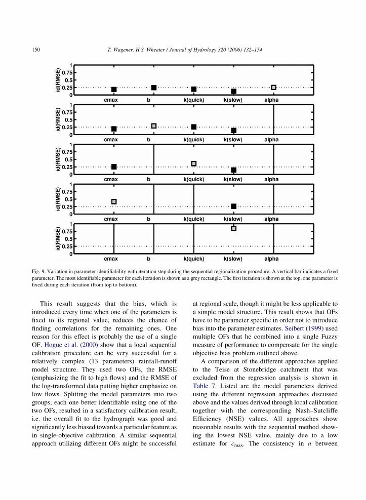
Fig. 9. Variation in parameter identifiability with iteration step during the sequential regionalization procedure. A vertical bar indicates a fixed

parameter. The most identifiable parameter for each iteration is shown as a grey rectangle. The first iteration is shown at the top, one parameter is

fixed during each iteration (from top to bottom).

T. Wagener, H.S. Wheater / Journal of Hydrology 320 (2006) 132–154150

This result suggests that the bias, which is

introduced every time when one of the parameters is

fixed to its regional value, reduces the chance of

finding correlations for the remaining ones. One

reason for this effect is probably the use of a single

OF. Hogue et al. (2000) show that a local sequential

calibration procedure can be very successful for a

relatively complex (13 parameters) rainfall-runoff

model structure. They used two OFs, the RMSE

(emphasizing the fit to high flows) and the RMSE of

the log-transformed data putting higher emphasize on

low flows. Splitting the model parameters into two

groups, each one better identifiable using one of the

two OFs, resulted in a satisfactory calibration result,

i.e. the overall fit to the hydrograph was good and

significantly less biased towards a particular feature as

in single-objective calibration. A similar sequential

approach utilizing different OFs might be successful

at regional scale, though it might be less applicable to

a simple model structure. This result shows that OFs

have to be parameter specific in order not to introduce

bias into the parameter estimates. Seibert (1999) used

multiple OFs that he combined into a single Fuzzy

measure of performance to compensate for the single

objective bias problem outlined above.

A comparison of the different approaches applied

to the Teise at Stonebridge catchment that was

excluded from the regression analysis is shown in

Table 7. Listed are the model parameters derived

using the different regression approaches discussed

above and the values derived through local calibration

together with the corresponding Nash–Sutcliffe

Efficiency (NSE) values. All approaches show

reasonable results with the sequential method show-

ing the lowest NSE value, mainly due to a low

estimate for cmax. The consistency in a between

Table 7

Comparison of regionalized and locally calibrated parameter values for the Teise at Stoenbridge

Approach cmax b kquick kslow a NSE*

Local calibration 316.5 0.125 1.66 92.1 0.72 0.79

Conventional

regression

304.4 0.181 2.61 190.4 0.72 0.78

Weighted

regression

306.5 0.158 2.60 148.8 0.74 0.78

Sequential

regression

227.2 0.162 2.70 197.9 0.72 0.76

*Nash–sutcliffe efficiency.

T. Wagener, H.S. Wheater / Journal of Hydrology 320 (2006) 132–154 151

the approaches underlines the high identifiability and

strong correlation with catchment characteristics of

this parameter. Future studies with a larger number of

catchments will provide a better measure of compari-

son between the approaches.

4. Conclusions

The prediction of the hydrologic response of

ungauged catchments is a fundamental problem in

hydrology. One of the approaches to solve it is to

apply a model to a large number of gauged catchments

and to derive statistical relationships between model

parameters and catchment characteristics, so called

regionalization. This has so far been done with only

limited success, particularly for continuous simulation

models. Some aspects that limit the success of this

type of approach are discussed and evaluated in this

paper, and potential ways forward are suggested. The

main conclusions of this paper are as follows:

The dominating catchment descriptor separating

the different response types of the study catch-

ments is the baseflow index.

The benchmark regionalization shows a typical

result with only a few parameters showing any

sizeable amount of correlation with catchment

characteristics.

Embedding a particular model component within

two different model structures resulted in different

optimal parameter values for this component. This

result suggests that parameter interaction during

calibration can hinder the identification of a

parameter in a way that considers its intended

(functional) role in the model. The latter being a

necessary condition for successful regionalization.

The results of this study suggest that the

identifiability of a parameter is related to its

importance in representing the catchment’s

response. A weighted regression procedure has

been proposed to avoid giving well and poorly

identified parameters the same weight during

regionalization.

Many regionalization studies contain outliers, i.e.

one parameter shows a clear correlation with a

particular catchment characteristic, but one of the

catchments is behaving differently. This catchment

should be taken out of the analysis and investigated

separately. One therefore derives a better regiona-

lization relationship, which will however fail for

certain cases.

Model structural error introduces ambiguity into

the identification of optimum parameter values.

This ambiguity is propagated into the regionaliza-

tion and different regional relationship will some-

times be found for the same parameter when

optimizing the model to different parts of the

hydrograph. This was found to be true here for the

quick flow time constant, which was either related

to the topography (during high flows) or to rainfall

characteristics (during low flows).

Sequential regionalization procedures are useful in

increasing the identifiability of parameters. How-

ever, there is a danger of introducing bias into the

calibration and therefore into the regional relation-

ships. Additional research is required to develop

appropriate procedures of this type for relatively

simple model structures.

The conclusions listed above focus on the

procedures applied in this study and their

T. Wagener, H.S. Wheater / Journal of Hydrology 320 (2006) 132–154152

underlying assumptions. The exact values derived

are unlikely to be very robust due to the small

number of catchments that was available. The

results were, however, sufficient to provide a

general trend. A more extensive study with a

larger number of catchments is currently in

progress. In conclusion, we note that recent years

have shown an increased interest in the modeling

of ungauged catchments using continuous rainfall-

runoff models. However, many unanswered ques-

tions remain for the time being. In addition,

progress in parameter estimation procedures and

parsimonious modelling still have to be fully

incorporated into regionalization approaches. This

study demonstrated that care has to be taken during

the model calibration stage if meaningful results

are to be obtained during regionalization. Of

particular importance is the functional role of the

parameter within the model that has to be

maintained if meaningful relationships to catchment

characteristics are the objective. This study

suggests that the functional role of parameters has

to be given equal importance to model performance

in MOPEX comparison studies.

Acknowledgements

This project was funded by NERC grant

GR3/11653. Partial support for the first author was

provided by a fellowship of the German Academic

Exchange Service (DAAD) and by SAHRA (Sustain-

ability of semi-Arid Hydrology and Riparian Areas)

under the STC Program of the National Science

Foundation, Agreement No. EAR-9876800. Figures

reprinted from Wagener et al. (2004) with permission

of Imperial College Press. We thank the two

anonymous reviewers for their very thoughtful

comments that helped improve the quality of the

paper.

Appendix A

The identifiability measure introduced in the main

text can be used as a weight in a regression model to

enhance the influence of better-identified parameters

on the final regional model. This can be written in

mathematical form as weighted linear regression (e.g.

Weisberg, 1980, p. 75f.). Starting with the standard

regression model,

qL Z FqR C3R (10)

the generalized least squares solution is given by

qR Z ðFT LK1FÞK1FTLK1qL (11)

in case of a weighted least squares, where a higher

weight indicates a more precise estimate. The

weighting function L can be written as

L Z

wK11

wK12 0

1

0 wK1n

2666664

3777775 (12)

one can then define an n!n matrix, C, for which

CTCZLK1. C is called the square root of LK1.

Subsequently C is

C Z

ffiffiffiffiffiffiw1

p

ffiffiffiffiffiffiw2

p0

1

0ffiffiffiffiffiffiwn

p

266664

377775 (13)

which can be transformed into an ordinary least

squares problem by multiplying both sides of Eq. 10

by C, which leads to

CqL Z CFqR CC3R (14)

one can then define ZZCqL, W ZCF and dZC3R,

leading to

Z Z WqR Cd (15)

with the ordinary least squares solution being

qR Z ðWT WÞK1WT Z (16)

An ordinary or unweighted least squares problem

is therefore obtained from a weighted least squares

problem through transformation of all the involved

variables. Each observation of dependent and inde-

pendent variables, and the intercept term (which is a

column of ones, added to the matrix of independent

variables) has to be multiplied by the square root of

the weight for that pointffiffiffiffiffiwi

p. Estimates of the

parameters, tests, confidence intervals, and residuals

T. Wagener, H.S. Wheater / Journal of Hydrology 320 (2006) 132–154 153

can then be derived using ordinary least squares as

described earlier (e.g. Weisberg, 1980, p. 76).

References

Abdulla, F.A., Lettenmaier, D.P., 1997. Development of regional

parameter estimation equations for a macroscale hydrologic

model. J. Hydrol. 197, 230–257.

Atkinson, S.E., Woods, R.A., Sivapalan, M., 2002. Climate and

landscape controls on water balance model complexity over

changing timescales. Water Resour. Res. 38 (12).

101029/2002WR001487.

Bayliss, A., 1999. Flood Estimation Handbook-5: Catchment

Descriptors. Institute of Hydrology, Wallingford.

Beven, K.J., 2000. Uniqueness of place and process representations

in hydrological modelling. Hydrol. Earth Sys. Sci. 4 (2), 203–

213.

Beven, K.J., Franks, S.W., 1999. Functional similarity in landscape

scale SVAT modeling. Hydrol. Earth Sys. Sci. 3 (1), 85–94.

Beven, K.J., Freer, J., Hankin, B., Schulz, K., 2000. The use of

generalized likelihood measures for uncertainty estimation in

higher-order models of environmental systems. In: Fitzgerald,

Smith, R.C., Walden, A.T., Young, P.C. (Eds.), Nonlinear and

Nonstationary Signal Processing. Cambridge University Press,

UK.

Blazkova, S., Beven, K.J., 2002. Flood frequency estimation by

continuous simulation for a catchment treated as ungauged

(with uncertainty). Water Resour. Res. 38 (8), 10.

Boyle, D.P., Gupta, H.V., Sorooshian, S., 2000. Toward improved

calibration of hydrological models: combining the strengths of

manual and automatic methods. Water Resour. Res. 36 (12),

3663–3674.

Cameron, D., Beven, K.J., Tawn, J., 2001. Modelling extreme

rainfalls using a modified random pulse Bartlett-Lewis

stochastic rainfall model (with uncertainty). Adv. Water Resour.

24, 203–211.

Dingman, S.L., 1994. Physical Hydrology. Prentice Hall, Engle-

wood Cliffs, NJ.

Duan, Q., Schaake, J., Koren, V., 2001. A priori estimation of land

surface model parameters. In Lakshmi, V., Albertson, J.,

Schaake, J. (eds). Land surface hydrology, meteorology, and

climate: Observations and modelling. American Geophysical

Union, Water Science and Application, vol. 3, 77-94.

Dunne, S.M., 1999. Imposing constraints on parameter values of a

conceptual hydrological model using baseflow response.

Hydrol. Earth Sys. Sci. 3, 271–284.

Evans, J.P., Jakeman, A.J., 1998. Development of a simple,

catchment-scale, rainfall-evapotranspiration-runoff model.

Env. Mod. Software 13, 385–393.

FEH (Flood Estimation Handbook) 1999. Catchment character-

istics.CD Publication.

Fernandez, W., Vogel, R.M., Sankarasubramanian, S., 2000.

Regional calibration of a watershed model. Hydrol. Sci. J. 45

(5), 689–707.

Gan, T.Y., Burges, S.J., 1990. An assessment of a conceptual

rainfall-runoff models ability to represent the dynamics of small

hypothetical catchments 2. Hydrologic responses for normal and

extreme rainfall. Water Resour. Res. 26 (7), 1605–1619.

Gershenfeld, N., 1999. The Nature of Mathematical Modelling.

Cambridge University Press, Cambridge.

Gupta, H.V., Sorooshian, S., Yapo, P.O., 1998. Toward improved

calibration of hydrologic models: multiple and noncommensur-

able measures of information. Water Resour. Res. 34 (4), 751–

763.

Gupta, H.V., Beven, K.J., Wagener, T. 2004. Model calibration and

uncertainty estimation. In Andersen, M. (ed.) Encyclopedia of

Hydrological Sciences. In Press.

Hogue, T.S., Sorooshian, S., Gupta, H.V., Holz, A., Braatz, D.,

2000. A multistep automatic calibration scheme for river

forecasting models. J. Hydromet. 1, 524–542.

Houghton-Carr, H., 1999. Flood Estimation Handbook-4: Restate-

ment and Application of the Flood Studies Report Rainfall-

runoff Method. Institute of Hydrology, Wallingford.

Jakeman, A.J., Hornberger, G.M., Littlewood, I.G., Whitehead,

P.G., Harvey, J.W., Bencala, K.E., 1992. A systematic approach

to modelling the dynamic linkage of climate, physical

catchment descriptors and hydrological response components.

Math. Comp. Sim. 33, 359–366.

Jakeman, A.J., Hornberger, G.M., 1993. How much complexity is

warranted in a rainfall-runoff model? Water Resour. Res. 29 (8),

2637–2649.

Jakeman, A.J., Chen, T.H., Post, D.A., Hornberger, G.M., Little-

wood, I.G., Whitehead, P.G., 1993. Assessing uncertainties in

hydrological response to climate at large scale. Macroscale

modelling of the hydrosphere.. Proceedings of the Yokohama

Symposium, IAHS Publication No. 214, 37–47.

Kokkonen, T.S., Jakeman, A.J., 2001. A comparison of metric and

conceptual approaches in rainfall-runoff modelling and its

implications. Water Resour. Res. 37 (9), 2345–2352.

Koren, V.I., Smith, M., Wang, D., Zhang, Z., 2000. Use of soil

property data in the derivation of conceptual rainfall-runoff

model parameters, 15th Conference on Hydrology, Long Beach.

American Meteorological Society, USA (Paper 2.16).

Kottegoda, N.T., Rosso, R., 1997. Statistics, probability, and

reliability for civil and environmental engineers. McGraw-

Hill, New York, USA.

Lamb, R., Beven, K.J., Myrabo, S., 1998. Use of spatially

distributed water table observations to constrain uncertainity

in a rainfall-runoff model. Advances in Water Resources 22(4),

305–317.

Lamb, R., Calver, A., 2002. Continuous simulation as a basis for

national flood frequency estimation. In Littlewood I. (ed).

Continuous river flow simulation: methods, applications and

uncertainties,.BHS—Occasional Papers, No. 13, Wallingford;

67–75.

Lamb, R., Crewett, J., Calver, A, 2000. Relating hydrological model

parameters and catchment properties to estimate flood

frequencies from simulated river flows, BHS 7th National

Hydrology Symposium, Newcastle-upon-Tyne, 7, 357–364

T. Wagener, H.S. Wheater / Journal of Hydrology 320 (2006) 132–154154

Lamb, R., 2000. An approach to the calibration of a conceptual

rainfall-runoff model for flood frequency estimation by

continuous simulation. Water Resour. Res. 35, 3103–3114.

Lamb, R., Kay, A.L., 2004. Confidence intervals for a spatially

generalized, continuous simulation flood frequency model for

Great Britain. Water Resour. Res. 40, W07501 doi:

10.1029/2003WR002428.

Linsley Jr.., R.K., Kohler, M.A., Paulhus, J.L.H., 1949. Applied

Hydrology. McGraw-Hill, New York.

Merz, B., Bloschl, G., 2004. Regionalisation of catchment model

parameters. J. Hydrol. 287 (1–4), 95–123.

McCuen, R.H., 1982. A Guide to Hydrologic Analysis Using SCS

Methods. Prentice-Hall, Englewood Cliffs, NJ, USA.

McGlynn, B.L., McDonnell, J.J., 2003. Quantifying the relative

contributions of riparian and hillslope zones to catchment runoff

and composition. Water Resour. Res. 39 (11), 1310.

10.1029/2003WR002091.

Moore, R.J., 1999. Real-time flood forecasting systems: perspec-

tives and prospects. In: Casale, R., Margottini, C. (Eds.), Floods

and Landslides: Integrated Risk Assessment. Springer-Verlag,

Berlin.

Mosley, M.P., 1981. Delimitation of New Zealand hydrologic

regions. J. Hydrol. 49, 173–192.

NERC, 1975.Anon., 1975. Flood Studies Report. Natural Environ-

ment Research Council, UK.

Pilgrim, D.H., 1983. Some problems in transferring hydrological

relationships between small and large drainage basins and

between regions. J. Hydrol. 65, 49–72.

Post, D.A., Jakeman, A.J., 1996. Relationships between physical

attributes and hydrologic response characteristics in small

Australian mountain ash catchments. Hydrol. Proc. 10, 877–

892.

Post, D.A., Jones, J.A., Grant, G.E., 1998. An improved

methodology for predicting the daily hydrologic response of

ungauged catchments. Env. Mod. Software 13, 395–403.

Sefton, C.E.M., Howarth, S.M., 1998. Relationships between

dynamic response characteristics and physical descriptors of

catchments in England and Wales. J. Hydrol. 211, 1–16.

Sefton, C.E.M., Whitehead, P.G., Eatherall, A., Littlewood, I.G.,

Jakeman, A.J., 1995. Dynamic response characteristics of

the Plynlimon catchments and preliminary analysis of

relationships to physical catchment descriptors. Environmetrics

6, 465–472.

Seibert, J., 1999. Regionalisation of parameters for a conceptual

rainfall-runoff model. Agric. Forest Meteor. 98–99, 279–293.

Sivapalan, M., Takeuchi, K., Franks, S.W., Gupta, V.K., Karambiri,

H., Lakshim, V., Liang, X., McDonnell, J.J., Mendiondo, E.M.,

Connell, O., Oki, T., Pomeroy, J.W., Schertzer, D., Uhlenbrook,

S., Zehe, E., 2003. IAHS Decade on Predictions in Ungauged

Basins (PUB), 2003-2012: Shaping an exciting future for the

hydrological sciences. Hydrol. Sci. J. 48 (6), 857–880.

Tung, Y.-K., Yeh, K.-C., Yang, J.-C., 1997. Regionalization of unit

hydrograph parameters: 1. Comparison of regression analysis

techniques. Stoch. Hydrol. Hydraulics 11, 145–171.

Vandewiele, G.L., Elias, A., 1995. Monthly water balance of

ungauged catchments obtained by geographical regionalization.

J. Hydrol. 170, 277–291.

Wagener, T., Boyle, D.P., Lees, M.J., Wheater, H.S., Gupta, H.V.,

Sorooshian, S., 2001. A framework for development and

application of hydrological models. Hydrol. Earth Syst. Sci. 5

(1), 13–26.

Wagener, T., Lees, M.J., Wheater, H.S., 2002. A toolkit for the

development and application of parsimonious hydrological

models. In: Singh, V.P., Frevert, D. (Eds.), Mathematical

Models of Large Watershed Hydrology, vol. 1. Water Resources

Publishers, USA, pp. 87–136.

Wagener, T., Wheater, H.S., Gupta, H.V., 2004. Rainfall-Runoff

Modelling in Gauged and Ungauged Catchments. Imperial

College Press, London p. 300.

Weisberg, S., 1980. Applied linear regression. John Wiley & Sons,

Chichester, UK

Wheater, H.S., Jakeman, A.J., Beven, K.J., 1993. Progress and

directions in rainfall-runoff modelling. In: Jakeman, A.J., Beck,

M.B., McAleer, M.J. (Eds.), Modelling Change in Environ-

mental Systems. Wiley, Chichester, pp. 101–132.

Yapo, P.O., Gupta, H.V., Sorooshian, S., 1996. Automatic

calibration of conceptual rainfall-runoff models: sensitivity to

calibration data. J. Hydrol. 181, 23–48.

Young, A., 2002. River flow simulation within ungauged

catchments using a daily rainfall-runoff model, In Littlewood

I. (ed). Continuous river flow simulation: Methods, applications

and uncertainties, BHS-Occasional Papers, No.13 (2002) 31–38