parameter estimation for dark energy models
TRANSCRIPT

PARAMETER ESTIMATION for DARK ENERGY MODELS
using SN1a and other data sets
Report for the presentation delivered on the same topic as a part of the course PHYS601
August 2012
BY : ARSHDEEP SINGH BHATIA
Department of Physics and Astrophysics
University of Delhi

LIKELIHOOD ANALYSIS
• Likelihood Analysis is a statistical technique which allows us to estimate the values of free parameters in an assumed model (Hypotheses), given a set of observed data to test our model upon.
• A likelihood function (L.F.) for the parameters is obtained which acts as pdf for the parameters.
• The analysis is based on Likelihood principle which states that the L.F. exhausts all the information contained in the observations related to the parameters.
Bayesian Approach
• Given a set of parameters ‘θ’ , a Hypotheses ‘H’ and a set of Data ‘D’ , one is interested in finding p({θ}|D,H)
• Baye’s Theorem allows us to relate p({θ}|D,H) to calculable probability p(D|{θ},H) as :
Here p(D|{θ},H) is called the likelihood (of the data, given a set of parameters) p({θ}|D,H) is posterior probability (the state of knowledge , given a data)

p({θ}|H) is called the prior (what is known about parameters before the experiment p(D|H) is called the evidence, and is usually ignored as it is independent of parameters For a flat prior(constant), Bayes’s Theorem can be written as
Where L(D|{θ}) is the likelihood
• What is essentially done is minimization of chi statistic wrt model parameters, where
DARK ENERGY MODEL UNDER CONSIDERATION
We consider a Multiple K-essence model and also a sub – class of this, as proposed in two of our earlier works:
• S. Sur and S. Das, JCAP 0901 007 (2009) • S. Sur , arXiv 0902.1186 (2009)
and some more work in progress. Normalized Hubble’s Parameter for the model

In the model :
• ‘a’ is the cosmological scale factor • Parameter is assigned value 1 or 2 • H0 is the Hubble’s constant
Marginalization is to be done over the three model parameters :
1. A 2. B 3. Ω0m : present value of matter density parameter
Data Being Used (Supernova 1a, CMB, BAO)
• We use SN 1a Union Data : M. Kowalski et al, Astrophys J. 686 749 (2008), and subsequent works.
• It consists of 307 most reliable data points that range up to red shift ~ 1.7, and include large samples of SN 1a from older data sets, high-z Hubble Space Telescope (HST) observations and SN Legacy Survey (SNLS)
• The SN 1a data provides the observed distance modulus, μobs(zi), with respective 1σ uncertainties, σi, for SN 1a located at various red-shifts.
• CMB + BAO results were obtained from Wilkinson Microwave Anisotropy Probe (WMAP) and Sloan Digital Sky Survey (SDSS).

FINDING THE BEST FIT VALUES FOR THE MODEL PARAMETERS We find χ2 statistic for physical quantities whose theoretical value depend explicitly or implicitly on the model parameters.
Yi = observed value Yexp = estimated value from the model σi = 1σ error in the observed value n = no. of data points
• Minimization of χ2 statistic yields the best fit values for the model parameters We find the independent χ2 statistic for our model using the following observations
1. Distance Modulus from Supernovae 1a data 2. CMB shift parameter 3. BAO peak distance parameter

1. Supernovae Analysis
• Supernovae of type 1a (SN1a) are STANDARD CANDLES , a fact which can be used to calculate the distance of the SN using their observed brightness.
• χ2 statistic for these set of values is given by:
where, n= number of data points
Where ‘h’ is hubble constant in Km/h Mpc

2. CMB Data
• The observable here is the CMB shift parameter ‘R’, whose predicted value from theory is:
With χ2 statistic given by:
• The numerical values of Z* and Robs are provided by WMAP five year data.
3. BAO peak distance Data
• The third observable was BAO peak distance parameter, ‘A’ from SDSS luminous red galaxies , whose observed value is again given by WMAP five year data.
• The theoretical value of the parameter is given by the expression :

with zb = 0.35 and
TOTAL χ2 The total χ2 statistic is given by:
• We do a minimization of the above expression for total χ2 wrt all the 3 model parameters, using a code written in Mathematica.
• Best fit values of parameter are found to be:
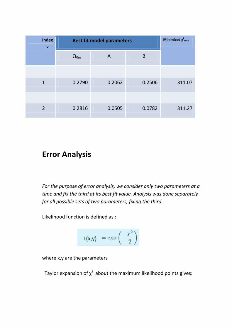
Index ν
Best fit model parameters Minimized χ2total
Ω0m A B
1 0.2790 0.2062 0.2506 311.07
2 0.2816 0.0505 0.0782 311.27
Error Analysis
For the purpose of error analysis, we consider only two parameters at a time and fix the third at its best fit value. Analysis was done separately for all possible sets of two parameters, fixing the third. Likelihood function is defined as :
where x,y are the parameters Taylor expansion of χ2 about the maximum likelihood points gives:

Where explicit use of FISHER MATRIX [F] has been made:
[C] is the covariance matrix , which gives sigma errors in x,y and the correlation between the parameters.
• Comparing the final form of ‘L’ with :
which is a normal distribution function in two parameters shows us that the likelihood is normally distributed with best fit parameter points as the mean.
• Hence results of normal distribution can be carried over to Likelihood function

• As in generally done in case of normal distributions, we find the 1- σ, 2- σ errors . These correspond to contours of a fixed probability/likelihood in the parameter space.
• As can be seen from the definition of likelihood ‘L’, contours of constant likelihood in parameter space correspond to contours of a fixed χ2 in the parameter space.
Which represents an ellipse in x,y space.
• These ellipses are concentric, as can be seen from the above equation, with points of maximum likelihood as their centre.
• These ellipses have axis which are rotated wrt coordinate axis at fixed angle which is dependent on the correlation between the parameters. Parameters with null correlation yield ellipses whose axis are parallel to coordinate axis.

1σ , 2σ and 3σ contours in parameter space (for best fit value of Ω0m ), for υ =1 & 2 respectively.
• The innermost ellipse is the bound for 1σ error region and the next ellipse binds the 2σ region and so on.
• The dot in the middle of the 1σ plot represents the best fit value of the parameters obtained.

1σ , 2σ and 3σ contours in parameter space (for best fit value of B & A), for υ =1 & 2 respectively.

• The innermost ellipse is the bound for 1σ error region and the next ellipse binds the 2σ region and so on.
• The dot in the middle of the 1σ plot represents the best fit value of the parameters obtained.
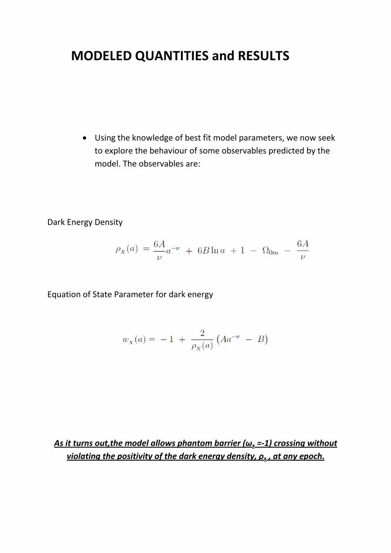
MODELED QUANTITIES and RESULTS
• Using the knowledge of best fit model parameters, we now seek to explore the behaviour of some observables predicted by the model. The observables are:
Dark Energy Density
Equation of State Parameter for dark energy
As it turns out,the model allows phantom barrier (ωx =-1) crossing without violating the positivity of the dark energy density, ρx , at any epoch.

Evolution of ωx(z) and ρx (z) with ν =1
Evolution of ωx(z) and ρx (z) , taking the best fit values of free parameters obtained for υ=1. zc denotes the red-shift at which ωx = -1 line is crossed. ω0x
and ρ0x are values of ωx and ρx at present epoch (z=0). The shaded region shows the 1σ error region

Evolution of ωx(z) and ρx (z) with ν =2
Evolution of ωx(z) and ρx (z) , taking the best fit values of free parameters obtained for υ=2. zc denotes the red-shift at which ωx = -1 line is crossed. ω0x
and ρ0x are values of ωx and ρx at present epoch (z=0). The shaded region shows the 1σ error region.
SUMMARY
Given a theoretical model, likelihood analysis can be used to estimate the values of model parameters.
A dark energy model was considered which had 3 model parameters.
SN1a, CMB and BAO data was used as observed data.
χ2 statistic was calculated using observed data and theoretical values predicted by the model under consideration ,and was marginalized over the 3 model parameters to obtain best fit values of those parameters.
σ errors and likelihood plots for the model parameters were computed.
Observables predicted by the model were computed, along with corresponding errors, using the knowledge of model parameter values.