parameter identi–cation in an estimated new keynesian ... · prior research on identi–cation...

Parameter Identi�cation in an Estimated NewKeynesian Open Economy Model

Malin Adolfson, Sveriges RiksbankJesper Lindé, Federal Reserve Board

Macroeconomic Modeling Workshop

Jerusalem

October 28, 2009

Introduction

Vast interest in estimating and using DSGE models for policyanalysis in recent years

Fed, ECB, IMF, Riksbank etc.

Econometric methodology

Bayesian estimation widespread:

combine prior information and information from the likelihoodfunctionprovides curvature to the likelihood

Maximum likelihood unpopular:

hard to get plausible results

But recently DSGE models questioned in terms of identi�cation

Prior research on identi�cation

Canova and Sala (2009)

Limited information methods (match impulse response functions)Observational equivalence and weak identi�cation problems

Iskrev (2008, 2009)

Likelihood based methodsTest identi�cation based on the Information (Hessian) matrixDi¤erentiate between information in the data and structure of themodel

Weak identi�cation

Large sample required to obtain reliable estimatesLikelihood function invariant w.r.t a particular parameter(observational equivalence)

What we do

Parameter identi�cation in an open economy DSGE

Adolfson et al. (JEDC, 2008)

estimated on Swedish data with Bayesian techniquesmodel similar to Smets and Wouters (2003)=) results relevant for many models

Use Monte Carlo methods:

ML estimation on arti�cal samples- generated from posterior estimates from actual dataDi¤erent sample sizes and sets of observed variables

Value added:

Assess properties of the ML estimatorQuantify the economic signi�cance of weak identi�cationStudy accuracy of inverse Hessian

ML estimation on actual data (case study)

Key �ndings

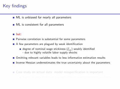
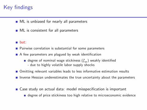
ML is unbiased for nearly all parameters

ML is consistent for all parameters

but:

Pairwise correlation is substantial for some parameters

A few parameters are plagued by weak identi�cation

degree of nominal wage stickiness (ξw ) weakly identi�ed- due to highly volatile labor supply shocks

Omitting relevant variables leads to less informative estimation results

Inverse Hessian underestimates the true uncertainty about the parameters

Case study on actual data: model misspeci�cation is important

degree of price stickiness too high relative to microeconomic evidence

Overview

1 The DGP - a New Keynesian open economy DSGE model

2 The Monte-Carlo simulation setup

3 Simulation results

4 ML estimation on actual data

5 Concluding remarks

Data Generating Process

The model is an open economy version of CEE (2005)

Consumption and investment baskets (domestic and imported goods)Incomplete exchange rate pass-through (LCP)Stochastic unit-root technology shock (Altig et al., 2003)SOE assumption: foreign economy exogenous

Parameterization

Bayesian estimation using Swedish data on 15 variables:

Yt=[πdt ∆ ln (W t/Pt ) ∆ lnCt ∆ ln It xt it Ht

∆ lnYt ∆ ln Xt ∆ ln Mt πcpit πdef ,it ∆ lnY �t π�t R�t ]0.

Steady-state parameters calibratedDynamic parameters estimatedPosterior median used as true parameter values

DSGE model (closed economy aspects)

Households- Utility from consumption, leisure and real cash balances- Habit persistence (b)- Capital accumulation (investment adjustment costs, S 00)- Nominal wage stickiness (ξw ): Calvo, partial indexation (κw )

Domestic intermediate goods �rms- Cobb-Douglas (capital and labor)- Working capital- Price stickiness (ξd ): Calvo, partial indexation (κ)- Markup (λd )

Exogenous �scal policy- preestimated VAR(2) for taxes and gov. expenditures

MALADO

Blyertspenna

DSGE model (open economy aspects)

Consumption and investment CES baskets- ηi sub. elast. invest. goods- ηc sub. elast. cons. goods (calibrated)

Importing (consumption, investment) and exporting �rms- ηf sub. elast. foreign goods- Brand naming technology, markup (λm,c , λm,i )- Local currency price setting- Price stickiness (ξm,c , ξm,i , ξx ): Calvo, partial indexation - κ) incomplete pass-through

Trade in foreign bonds with partly endogenous risk-premium- φ nfa response, φs exchange rate response

Foreign economy exogenous- preestimated VAR(4) for [π�t , y

�t , R

�t ]

DSGE model (monetary policy)

Taylor type instrument rule:

bit = ρRbit�1 + (1� ρR )

�bπct + rπ �πct�1 � bπct �+ ry yt�1 + rx xt�1�+r∆π∆πct + r∆y∆yt + εR ,t

yt trend output gap

Monetary policy shocks

εR ,t ,- i.i.d.πct - AR(1)Estimate σR and σπc (ρπc calib to 0.975)

DSGE model (estimated shocks)

Technology shocks (µz ,t , εt ), investment speci�c (Υt ), asymmetric(ez�t )- AR(1) processes: fρj ,σjg , j = fµz , ε, Υ, ez�gMarkup shocks (λdt ,λ

m,ct ,λm,it ,λxt )

- i.i.d. fσd , σm,c , σm,i , σx g

Preference shocks (ζct , ζht )

- AR(1) processes: {ρj , σjg , j = {ζc ,ζhg

Risk premium shock (eφt )- AR(1) process: {ρφ, σφg

The Monte-Carlo simulation setup

1 Solve DSGE model using posterior median and calibrated parameters

2 Generate an arti�cial sample of length T

By simulating the model 1000+ T periodsInnovations drawn from the normal distribution (seed = 1, ...,N)

3 Estimate parameters by maximizing the likelihood function

Same set of observable variables as on actual dataCalibrated parameters and the �scal and foreign VARs are �xed atthe �true�values

4 Store parameter estimates, likelihood function value, inverseHessian, seed number and convergence diagnostics

5 Repeat this N times

to obtain a distribution that is roughly stableN = 1500

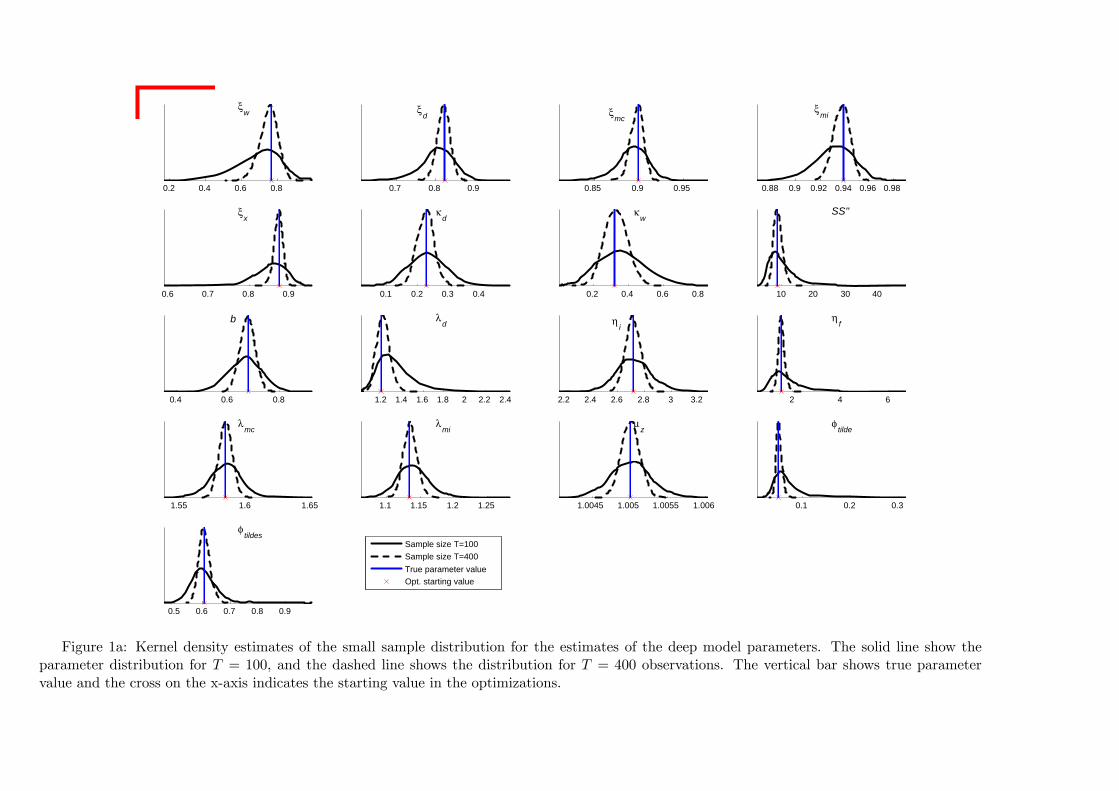
Simulation results

Study results for T = 100 observations and T = 400 observations inN samples

True values used to initiate each optimizationOut of 1, 500 simulations, the optimizations converged in 1, 452 cases

0.2 0.4 0.6 0.8

ξw

0.7 0.8 0.9

ξd

0.85 0.9 0.95

ξmc

0.88 0.9 0.92 0.94 0.96 0.98

ξmi

0.6 0.7 0.8 0.9

ξx

0.1 0.2 0.3 0.4

κd

0.2 0.4 0.6 0.8

κw

10 20 30 40

SS''

0.4 0.6 0.8

b

1.2 1.4 1.6 1.8 2 2.2 2.4

λd

2.2 2.4 2.6 2.8 3 3.2

ηi

2 4 6

ηf

1.55 1.6 1.65

λmc

1.1 1.15 1.2 1.25

λmi

1.0045 1.005 1.0055 1.006

μz

0.1 0.2 0.3

φtilde

0.5 0.6 0.7 0.8 0.9

φtildes

Sample size T=100Sample size T=400True parameter valueOpt. starting value

Figure 1a: Kernel density estimates of the small sample distribution for the estimates of the deep model parameters. The solid line show theparameter distribution for T = 100, and the dashed line shows the distribution for T = 400 observations. The vertical bar shows true parametervalue and the cross on the x-axis indicates the starting value in the optimizations.

MALADO

Rektangel

0.2 0.4 0.6 0.8

ρμ

z

0.4 0.6 0.8

ρε

0.2 0.4 0.6 0.8

ρυ

0.2 0.4 0.6 0.8

ρφ

0.2 0.4 0.6 0.8

ρz

c

0.2 0.4 0.6 0.8

ρz

h

0.2 0.4 0.6 0.8

ρz*

0.1 0.2 0.3

σz

0.5 0.6 0.7 0.8 0.9

σε

0.8 1 1.2 1.4 1.6

σλ

mc

0.8 1 1.2 1.4 1.6

σλ

mi

0.6 0.8 1

σλ

d

0.2 0.4 0.6 0.8

σϒ

0.5 1 1.5 2 2.5

σφ

0.2 0.4 0.6

σz

c

0.2 0.3 0.4 0.5 0.6

σz

h

0.1 0.2 0.3

σz*

1 2 3

σλ

x


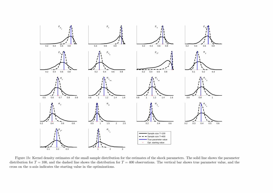
Figure 1b: Kernel density estimates of the small sample distribution for the estimates of the shock parameters. The solid line shows the parameterdistribution for T = 100, and the dashed line shows the distribution for T = 400 observations. The vertical bar shows true parameter value, and thecross on the x-axis indicates the starting value in the optimizations.

0.2 0.25 0.3

σR

0.2 0.4 0.6 0.8 1 1.2

σπ

bar

0.75 0.8 0.85 0.9 0.95

ρR

1 2 3 4 5

ln( rπ)

0 0.05 0.1 0.15 0.2 0.25

rΔπ

-1 -0.8 -0.6 -0.4 -0.2 0 0.2

rx

0 1 2 3 4

ry

0.1 0.2 0.3 0.4

rΔy


Figure 1c: Kernel density estimates of the small sample distribution for the estimates of the monetary policy parameters. The solid line showsthe parameter distribution for T = 100, and the dashed line show the distributions for T = 400 observations. The vertical bar shows true parametervalue, and the cross on the x-axis indicates the starting value in the optimizations.

MALADO

Rektangel

MALADO

Rektangel

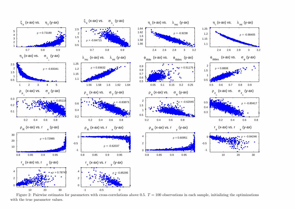
Pairwise correlation

Plotting pairwise parameter combinations with a correlationcoe¢ cient ρ > 0.5

Relatively strong degree of linear dependence within some regions ofthe parameter spaceNotice scale in the diagrams

0.7 0.8 0.912345

ξx (x-ax) vs. η

f (y-ax)

ρ = 0.73189

0.7 0.8 0.9

0.51

1.52

2.5

ξx (x-ax) vs. σ

λx

(y-ax)

ρ = -0.84715

2.4 2.6 2.8 3 3.2

1.561.58

1.61.621.64

ηi (x-ax) vs. λ

mc (y-ax)

ρ = -0.9238

2.4 2.6 2.8 3 3.2

1.1

1.15

1.2

1.25

ηi (x-ax) vs. λ

mi (y-ax)

ρ = -0.98405

1 2 3 4 5

0.51

1.52

2.5

ηf (x-ax) vs. σ

λx

(y-ax)

ρ = -0.83341

1.56 1.58 1.6 1.62 1.64

1.1

1.15

1.2

1.25

λmc

(x-ax) vs. λmi

(y-ax)

ρ = 0.93632

0.05 0.1 0.15 0.2 0.250.50.60.70.80.9

φtilde

(x-ax) vs. φtildes

(y-ax)

ρ = 0.51175

0.5 0.6 0.7 0.8 0.9

0.5

1

1.5

2

φtildes

(x-ax) vs. σφ (y-ax)

ρ = 0.8808

0.2 0.4 0.6 0.8

0.1

0.2

0.3

ρμ

z

(x-ax) vs. σz (y-ax)

ρ = -0.65118

0.2 0.4 0.6 0.80.2

0.4

0.6

ρυ (x-ax) vs. σ

ϒ (y-ax)

ρ = -0.83873

0.2 0.4 0.6 0.8

0.5

1

1.5

2

ρφ (x-ax) vs. σ

φ (y-ax)

ρ = -0.62045

0.2 0.4 0.6 0.8

0.3

0.4

0.5

ρz

h

(x-ax) vs. σz

h

(y-ax)

ρ = -0.80417

0.8 0.85 0.9 0.95

10

20

30

ρR

(x-ax) vs. rπ (y-ax)

ρ = 0.72985

0.8 0.85 0.9 0.95

-1

-0.5

0

ρR

(x-ax) vs. rx (y-ax)

ρ = -0.62037

0.8 0.85 0.9 0.95

0

2

4

ρR

(x-ax) vs. ry (y-ax)

ρ = 0.60951

10 20 30

-1

-0.5

0

rπ (x-ax) vs. r

x (y-ax)

ρ = -0.84246

10 20 30

0

2

4

rπ (x-ax) vs. r

y (y-ax)

ρ = 0.78742

-1 -0.5 0

0

2

4

rx (x-ax) vs. r

y (y-ax)

ρ = -0.85295

Figure 2: Pairwise estimates for parameters with cross-correlations above 0.5. T = 100 observations in each sample, initializing the optimizationswith the true parameter values.

MALADO

Rektangel

MALADO

Rektangel

0.7 0.8 0.912345

ξx (x-ax) vs. η

f (y-ax)

ρ = 0.73189

0.7 0.8 0.9

0.51

1.52

2.5

ξx (x-ax) vs. σ

λx

(y-ax)

ρ = -0.84715

2.4 2.6 2.8 3 3.2

1.561.58

1.61.621.64

ηi (x-ax) vs. λ

mc (y-ax)

ρ = -0.9238

2.4 2.6 2.8 3 3.2

1.1

1.15

1.2

1.25

ηi (x-ax) vs. λ

mi (y-ax)

ρ = -0.98405

1 2 3 4 5

0.51

1.52

2.5

ηf (x-ax) vs. σ

λx

(y-ax)

ρ = -0.83341

1.56 1.58 1.6 1.62 1.64

1.1

1.15

1.2

1.25

λmc

(x-ax) vs. λmi

(y-ax)

ρ = 0.93632

0.05 0.1 0.15 0.2 0.250.50.60.70.80.9

φtilde

(x-ax) vs. φtildes

(y-ax)

ρ = 0.51175

0.5 0.6 0.7 0.8 0.9

0.5

1

1.5

2

φtildes


ρ = 0.8808

0.2 0.4 0.6 0.8

0.1

0.2

0.3

ρμ

z


ρ = -0.65118

0.2 0.4 0.6 0.80.2

0.4

0.6

ρυ (x-ax) vs. σ

ϒ (y-ax)

ρ = -0.83873

0.2 0.4 0.6 0.8

0.5

1

1.5

2

ρφ (x-ax) vs. σ

φ (y-ax)

ρ = -0.62045

0.2 0.4 0.6 0.8

0.3

0.4

0.5

ρz

h

(x-ax) vs. σz

h

(y-ax)

ρ = -0.80417

0.8 0.85 0.9 0.95

10

20

30

ρR


ρ = 0.72985

0.8 0.85 0.9 0.95

-1

-0.5

0

ρR


ρ = -0.62037

0.8 0.85 0.9 0.95

0

2

4

ρR


ρ = 0.60951

10 20 30

-1

-0.5

0

rπ (x-ax) vs. r

x (y-ax)

ρ = -0.84246

10 20 30

0

2

4

rπ (x-ax) vs. r

y (y-ax)

ρ = 0.78742

-1 -0.5 0

0

2

4

rx (x-ax) vs. r

y (y-ax)

ρ = -0.85295


MALADO

Rektangel

0.7 0.8 0.912345

ξx (x-ax) vs. η

f (y-ax)

ρ = 0.73189

0.7 0.8 0.9

0.51

1.52

2.5

ξx (x-ax) vs. σ

λx

(y-ax)

ρ = -0.84715

2.4 2.6 2.8 3 3.2

1.561.58

1.61.621.64

ηi (x-ax) vs. λ

mc (y-ax)

ρ = -0.9238

2.4 2.6 2.8 3 3.2

1.1

1.15

1.2

1.25

ηi (x-ax) vs. λ

mi (y-ax)

ρ = -0.98405

1 2 3 4 5

0.51

1.52

2.5

ηf (x-ax) vs. σ

λx

(y-ax)

ρ = -0.83341

1.56 1.58 1.6 1.62 1.64

1.1

1.15

1.2

1.25

λmc

(x-ax) vs. λmi

(y-ax)

ρ = 0.93632

0.05 0.1 0.15 0.2 0.250.50.60.70.80.9

φtilde

(x-ax) vs. φtildes

(y-ax)

ρ = 0.51175

0.5 0.6 0.7 0.8 0.9

0.5

1

1.5

2

φtildes


ρ = 0.8808

0.2 0.4 0.6 0.8

0.1

0.2

0.3

ρμ

z


ρ = -0.65118

0.2 0.4 0.6 0.80.2

0.4

0.6

ρυ (x-ax) vs. σ

ϒ (y-ax)

ρ = -0.83873

0.2 0.4 0.6 0.8

0.5

1

1.5

2

ρφ (x-ax) vs. σ

φ (y-ax)

ρ = -0.62045

0.2 0.4 0.6 0.8

0.3

0.4

0.5

ρz

h

(x-ax) vs. σz

h

(y-ax)

ρ = -0.80417

0.8 0.85 0.9 0.95

10

20

30

ρR


ρ = 0.72985

0.8 0.85 0.9 0.95

-1

-0.5

0

ρR


ρ = -0.62037

0.8 0.85 0.9 0.95

0

2

4

ρR


ρ = 0.60951

10 20 30

-1

-0.5

0

rπ (x-ax) vs. r

x (y-ax)

ρ = -0.84246

10 20 30

0

2

4

rπ (x-ax) vs. r

y (y-ax)

ρ = 0.78742

-1 -0.5 0

0

2

4

rx (x-ax) vs. r

y (y-ax)

ρ = -0.85295


MALADO

Rektangel

MALADO

Rektangel

MALADO

Rektangel

Uncertainty underestimated

Standard deviations according to the inverse Hessian too small

underestimate the dispersion in the simulated distributions for someparameters

Table 3: Distribution results from different sample sizes.

100 observations 400 observations

Parameter True esti-

mates

Mean of distri-bution

Median of distri-bution

Std. of distri-bution

Median std. of inverse

Hessians

Mean of distri-bution

Median of distri-bution

Std. of distri-bution

Median std. of inverse

Hessians

Calvo wages wξ 0.77 0.74 0.75 0.13 0.07 0.76 0.76 0.05 0.03

Calvo domestic prices dξ 0.83 0.81 0.82 0.04 0.03 0.82 0.82 0.02 0.01

Calvo import cons. prices cm ,ξ 0.90 0.90 0.90 0.02 0.01 0.90 0.90 0.01 0.01

Calvo import inv. prices im ,ξ 0.94 0.94 0.94 0.02 0.01 0.94 0.94 0.01 0.01

Calvo export prices xξ 0.87 0.86 0.86 0.04 0.02 0.87 0.87 0.01 0.01

Indexation prices κ 0.23 0.22 0.22 0.06 0.05 0.22 0.22 0.03 0.02

Indexation wages wκ 0.32 0.32 0.32 0.15 0.07 0.32 0.32 0.07 0.04

Investment adj. cost ''~S 8.58 8.98 8.08 4.08 2.02 8.65 8.53 1.35 0.98

Habit formation b 0.68 0.67 0.67 0.07 0.05 0.68 0.68 0.03 0.02

Markup domestic dλ 1.20 1.21 1.20 0.14 0.09 1.20 1.19 0.06 0.04

Subst. elasticity invest. iη 2.72 2.72 2.71 0.13 0.11 2.71 2.71 0.06 0.05

Subst. elasticity foreign fη 1.53 1.59 1.45 0.59 0.23 1.54 1.53 0.14 0.09

Markup imported cons. cm ,λ 1.58 1.58 1.58 0.01 0.01 1.58 1.58 0.00 0.00

Markup.imported invest. im ,λ 1.13 1.14 1.13 0.02 0.02 1.13 1.13 0.01 0.01

Technology growth zμ 1.01 1.01 1.01 0.00 0.00 1.01 1.01 0.00 0.00

Risk premium φ~ 0.05 0.06 0.05 0.02 0.01 0.05 0.05 0.01 0.00

UIP modification sφ~ 0.61 0.61 0.60 0.05 0.03 0.61 0.61 0.02 0.01

Unit root tech. persistance zμρ 0.85 0.80 0.83 0.14 0.06 0.84 0.85 0.05 0.03

Stationary tech. persistance ερ 0.93 0.89 0.90 0.08 0.03 0.92 0.92 0.02 0.01

Invest. spec. tech. persist. Υρ 0.69 0.65 0.67 0.13 0.06 0.69 0.69 0.05 0.03

Risk premium persistence φρ ~ 0.68 0.65 0.65 0.11 0.06 0.68 0.68 0.04 0.03

Consumption pref. persist. cζρ 0.66 0.59 0.61 0.18 0.08 0.64 0.65 0.07 0.04

Labour supply persistance hζρ 0.27 0.26 0.26 0.13 0.07 0.27 0.27 0.06 0.04

Asymmetric tech. persist. *~zρ 0.96 0.73 0.84 0.28 0.09 0.93 0.95 0.11 0.02

Unit root tech. shock zμσ 0.13 0.14 0.14 0.05 0.03 0.13 0.13 0.02 0.01

Stationary tech. shock εσ 0.67 0.66 0.65 0.06 0.05 0.67 0.67 0.03 0.03

Imp. cons. markup shock cm ,λσ 1.13 1.13 1.12 0.11 0.10 1.13 1.13 0.05 0.05

Imp. invest. markup shock im ,λσ 1.13 1.14 1.13 0.11 0.10 1.14 1.14 0.05 0.05

Domestic markup shock dλσ 0.81 0.82 0.82 0.08 0.08 0.81 0.81 0.04 0.04

Invest. spec. tech. shock Υσ 0.40 0.42 0.41 0.09 0.06 0.40 0.40 0.03 0.02

Risk premium shock φσ ~ 0.79 0.82 0.80 0.21 0.12 0.80 0.80 0.08 0.06

Consumption pref. shock cζσ 0.26 0.27 0.27 0.05 0.04 0.27 0.26 0.02 0.02

Labour supply shock hζσ 0.39 0.39 0.39 0.06 0.04 0.38 0.38 0.03 0.02

Asymmetric tech. shock *~zσ 0.19 0.15 0.16 0.06 0.04 0.18 0.19 0.02 0.02

Export markup shock xλσ 1.03 1.13 1.09 0.41 0.21 1.04 1.03 0.11 0.08

Monetary policy shock Rσ 0.24 0.24 0.23 0.02 0.02 0.24 0.24 0.01 0.01

Inflation target shock cπσ 0.16 0.14 0.14 0.10 0.04 0.16 0.16 0.03 0.02

Interest rate smoothing Rρ 0.91 0.91 0.91 0.05 0.03 0.91 0.91 0.02 0.02

Inflation response πr 1.67 3.80 1.59 5.08 2.70 2.07 1.66 1.60 0.61

Diff. infl response πΔr 0.10 0.11 0.10 0.04 0.03 0.10 0.10 0.02 0.01

Real exch. rate response xr -0.02 -0.07 -0.02 0.15 0.02 -0.03 -0.02 0.04 0.01

Output response yr 0.13 0.35 0.13 0.63 0.07 0.17 0.13 0.17 0.04

Diff. output response yrΔ 0.18 0.19 0.18 0.05 0.03 0.18 0.18 0.02 0.02

Note: Out of the 1,500 estimations for the small sample (100 obs.), the results above is based on 1,452 convergent estimations with well behaved inverse Hessians. Out of the 1,500 estimations for the large sample (400 obs.), the results above is based on 1,497 convergent estimations with well behaved inverse Hessians. True parameter values were used as starting values in the estimations.

MALADO

Rektangel

MALADO

Rektangel

MALADO

Rektangel

MALADO

Rektangel

MALADO

Rektangel

MALADO

Rektangel

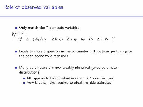
Role of observed variables

Only match the 7 domestic variables

Y subsett =[ πdt ∆ ln(Wt/Pt ) ∆ lnCt ∆ ln It Rt Ht ∆ lnYt ]0

Leads to more dispersion in the parameter distributions pertaining tothe open economy dimensions

Many parameters are now weakly identi�ed (wide parameterdistributions)

ML appears to be consistent even in the 7 variables caseVery large samples required to obtain reliable estimates

0.2 0.4 0.6 0.8

ξw

0.5 0.6 0.7 0.8 0.9

ξd

0.2 0.4 0.6 0.8

ξmc

0.2 0.4 0.6 0.8

ξmi

0.2 0.4 0.6 0.8

ξx

0.2 0.4 0.6 0.8

κd

0.2 0.4 0.6 0.8

κw

20 40 60 80

SS''

0.4 0.6 0.8

b

1.2 1.4 1.6 1.8 2 2.2 2.4

λd

2 4 6 8 10

ηi

5 10 15

ηf

1.5 2 2.5 3

λmc

1.5 2 2.5 3

λmi

1.002 1.004 1.006 1.008

μz

0.5 1 1.5 2

φtilde

0.2 0.4 0.6 0.8

φtildes

Benchmark set of observed variablesSmaller set of observed variablesTrue parameter value

Figure 3a: Kernel density estimates of the small sample distribution for the estimates of the deep model parameters. The solid line shows theparameter distributions when the estimations are based on the full set of observable variables, and the dashed line when the estimations are basedon fitting only a subset of variables (i.e., 7 “closed economy” variables). The true parameters are given by the vertical bars. T = 100 observations ineach of the N artificial samples, and we initialize the estimations by sampling parameters from the prior distributions in Table 2.

MALADO

Rektangel

MALADO

Rektangel

MALADO

Rektangel

MALADO

Rektangel

MALADO

Rektangel

MALADO

Rektangel

MALADO

Rektangel

MALADO

Rektangel

MALADO

Rektangel

MALADO

Rektangel

0.2 0.4 0.6 0.8

ρμ

z

0.2 0.4 0.6 0.8

ρε

0.2 0.4 0.6 0.8

ρυ

0.2 0.4 0.6 0.8

ρφ

0.2 0.4 0.6 0.8

ρz

c

0.2 0.4 0.6 0.8

ρz

h

0.2 0.4 0.6 0.8

ρz*

0.2 0.4 0.6 0.8 1

σz

0.5 1 1.5 2

σε

2 4 6 8 10

σλ

mc

2 4 6 8 10

σλ

mi

0.5 1 1.5 2

σλ

d

0.2 0.4 0.6 0.8

σϒ

1 2 3 4

σφ

0.2 0.4 0.6 0.8 1

σz

c

0.2 0.4 0.6 0.8 1 1.2 1.4

σz

h

0.5 1 1.5

σz*

1 2 3 4 5

σλ

x


Figure 3b: Kernel density estimates of the small sample distribution for the estimates of the shock parameters. The solid line shows the parameterdistribution when the estimations are based on the full set of observable variables, and the dashed line when the estimations are based on fitting onlya subset of variables (i.e., 7 “closed economy” variables). The true parameters are given by the vertical bars. T = 100 observations in each of the Nartificial samples, and we initialize the estimations by sampling parameters from the prior distributions in Table 2.

MALADO

Rektangel

MALADO

Rektangel

0.2 0.3 0.4 0.5

σR

0.2 0.4 0.6 0.8 1 1.2 1.4

σπ

bar

0.7 0.75 0.8 0.85 0.9 0.95

ρR

1 2 3 4 5

ln( rπ)

0 0.1 0.2 0.3 0.4

rΔπ

-2 -1 0 1 2

rx

0 1 2 3 4

ry

-0.2 0 0.2 0.4 0.6

rΔy


Figure 3c: Kernel density estimates of the small sample distribution for the estimates of the policy rule parameters. The solid line shows theparameter distribution when the estimations are based on the full set of observable variables, and the dashed line when the estimations are based onfitting only a subset of variables (i.e., 7 “closed economy” variables). The true parameters are given by the vertical bars. T = 100 observations ineach of the N artificial samples, and we initialize the estimations by sampling parameters from the prior distributions in Table 2.

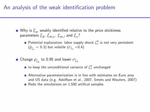
An analysis of the weak identi�cation problem

Why is ξw weakly identi�ed relative to the price stickinessparameters ξd , ξm,c , ξm,i and ξx ?

Potential explanation: labor supply shock ζht is not very persistent(ρζh

= 0.3) but volatile (σζh=0.4)

Change ρζhto 0.95 and lower σζh

to keep the unconditional variance of ζht unchanged

Alternative parameterization is in line with estimates on Euro areaand US data (e.g. Adolfson et al., 2007, Smets and Wouters, 2007)Redo the simulations on 1,500 arti�cal samples

Results from changing the labor supply shock process

Alternative parameterization facilitates identi�cation

The likelihood function is considerably more informative about ξw inthis case

but also more informative about the other deep parametersmatter less for the shock process parameters

Real wage series probably contaminated with measurement errors bythe way it is constructed

0.2 0.4 0.6 0.8

ξw

0.7 0.8 0.9

ξd

0.8 0.85 0.9 0.95

ξmc

0.8 0.85 0.9 0.95

ξmi

0.6 0.7 0.8 0.9

ξx

0.2 0.4 0.6 0.8

κd

0.2 0.4 0.6 0.8

κw

10 20 30 40 50

SS''

0.4 0.6 0.8

b

1.2 1.4 1.6 1.8 2 2.2 2.4

λd

2 2.5 3

ηi

2 4 6

ηf

1.3 1.4 1.5 1.6 1.7

λmc

1.1 1.2 1.3 1.4

λmi

1.004 1.005 1.006

μz

0.1 0.2 0.3

φtilde

0.2 0.4 0.6 0.8

φtildes

Benchmark specification of modelPersistent labor supply shocksTrue parameter value - benchmarkTrue par. val. - Persistent labor supply shocks

Figure 6a: Kernel density estimates of the small sample distribution for the estimates of the deep model parameters. The solid line showsthe benchmark parameter distribution, and the dashed line the distribution based on samples with more persistent labor supply shocks. The truebenchmark parameters are given by the solid vertical bars, and the true parameters used in the variant with more persistent labor supply shocks aregiven by the dashed vertical bars. T = 100 observations in each of the N artificial samples, and we initialize the estimations by sampling parametersfrom the prior distributions in Table 2.

MALADO

Rektangel

0.2 0.4 0.6 0.8

ρμ

z

0.4 0.6 0.8

ρε

0.2 0.4 0.6 0.8

ρυ

0.2 0.4 0.6 0.8

ρφ

0.2 0.4 0.6 0.8

ρz

c

0.2 0.4 0.6 0.8

ρz

h

0.2 0.4 0.6 0.8

ρz*

0.2 0.4 0.6 0.8 1

σz

0.5 1 1.5

σε

1 1.5 2 2.5

σλ

mc

1 1.5 2

σλ

mi

1 1.5 2

σλ

d

0.2 0.4 0.6 0.8 1

σϒ

1 2 3 4

σφ

0.2 0.4 0.6 0.8 1

σz

c

0.2 0.4 0.6 0.8 1

σz

h

0.2 0.4 0.6 0.8 1

σz*

1 2 3 4

σλ

x


Figure 6b: Kernel density estimates of the small sample distribution for the estimates of the shock parameters. The solid line shows thebenchmark parameter distribution, and the dashed line the distribution based on samples with more persistent labor supply shocks. The truebenchmark parameters are given by the solid vertical bars, and the true parameters used in the variant with more persistent labor supply shocks aregiven by the dashed vertical bars. T = 100 observations in each of the N artificial samples, and we initialize the estimations by sampling parametersfrom the prior distributions in Table 2.

MALADO

Rektangel

MALADO

Rektangel

0.15 0.2 0.25 0.3 0.35 0.4

σR

0.2 0.4 0.6 0.8 1 1.2

σπ

bar

0.75 0.8 0.85 0.9 0.95

ρR

1 2 3 4 5

ln( rπ)

-0.2 0 0.2 0.4

rΔπ

-1 -0.8 -0.6 -0.4 -0.2 0 0.2

rx

0 0.5 1 1.5 2 2.5 3

ry

-0.2 -0.1 0 0.1 0.2 0.3 0.4

rΔy


Figure 6c: Kernel density estimates of the small sample distribution for the estimates of the policy rule parameters. The solid line shows thebenchmark parameter distribution, and the dashed line the distribution based on samples with more persistent labor supply shocks. The truebenchmark parameters are given by the solid vertical bars, and the true parameters used in the variant with more persistent labor supply shocks aregiven by the dashed vertical bars. T = 100 observations in each of the N artificial samples, and we initialize the estimations by sampling parametersfrom the prior distributions in Table 2.

-8 -6 -4 -2 0 2 4 6

-10

-8

-6

-4

-2

0

2

4

6

8

(a) - Benchmark parameterization; ξw =0.765, ρzh

=0.27 and σzh

=0.386

Hours worked per capita

Rea

l wag

e

-8 -6 -4 -2 0 2 4 6

-10

-8

-6

-4

-2

0

2

4

6

8

(b) - Persistent labor supply shocks; ξw =0.765, ρzh

=0.95 and σzh

=0.125


Rea

l wag

e

-8 -6 -4 -2 0 2 4 6

-10

-8

-6

-4

-2

0

2

4

6

8

(c) - Flexible wages; ξw =0, ρzh

=0.27 and σ zh

=0.386


Rea

l wag

e

-8 -6 -4 -2 0 2 4 6

-10

-8

-6

-4

-2

0

2

4

6

8

Actual data, real wage stationarized with the HP-filter


Rea

l wag

e

20

40

60

80

100

120

140

160

180

200

Figure 5: Bivariate real wage and hours worked per capita scatter plots for benchmark (low persistence) and highly persistent labor supply shocksfor different degrees of nominal wage stickiness for a random sample of 200 observations. The ordering of the observations t = 1, 2, ..., 200 in thesample is indicated by the scale bar on the right hand side of the four panels.

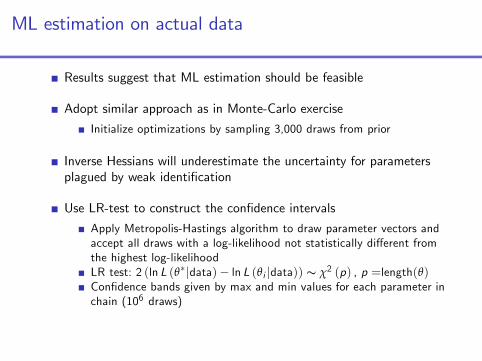
ML estimation on actual data

Results suggest that ML estimation should be feasible

Adopt similar approach as in Monte-Carlo exercise

Initialize optimizations by sampling 3,000 draws from prior

Inverse Hessians will underestimate the uncertainty for parametersplagued by weak identi�cation

Use LR-test to construct the con�dence intervals

Apply Metropolis-Hastings algorithm to draw parameter vectors andaccept all draws with a log-likelihood not statistically di¤erent fromthe highest log-likelihoodLR test: 2 (ln L (θ�jdata)� ln L (θi jdata)) s χ2 (p) , p =length(θ)Con�dence bands given by max and min values for each parameter inchain (106 draws)

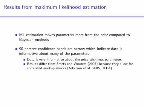
Results from maximum likelihood estimation

ML estimation moves parameters more from the prior compared toBayesian methods

90-percent con�dence bands are narrow which indicate data isinformative about many of the parameters

Data is very informative about the price stickiness parametersResults di¤er from Smets and Wouters (2007) because they allow forcorrelated markup shocks (Adolfson et al. 2005, JEEA)

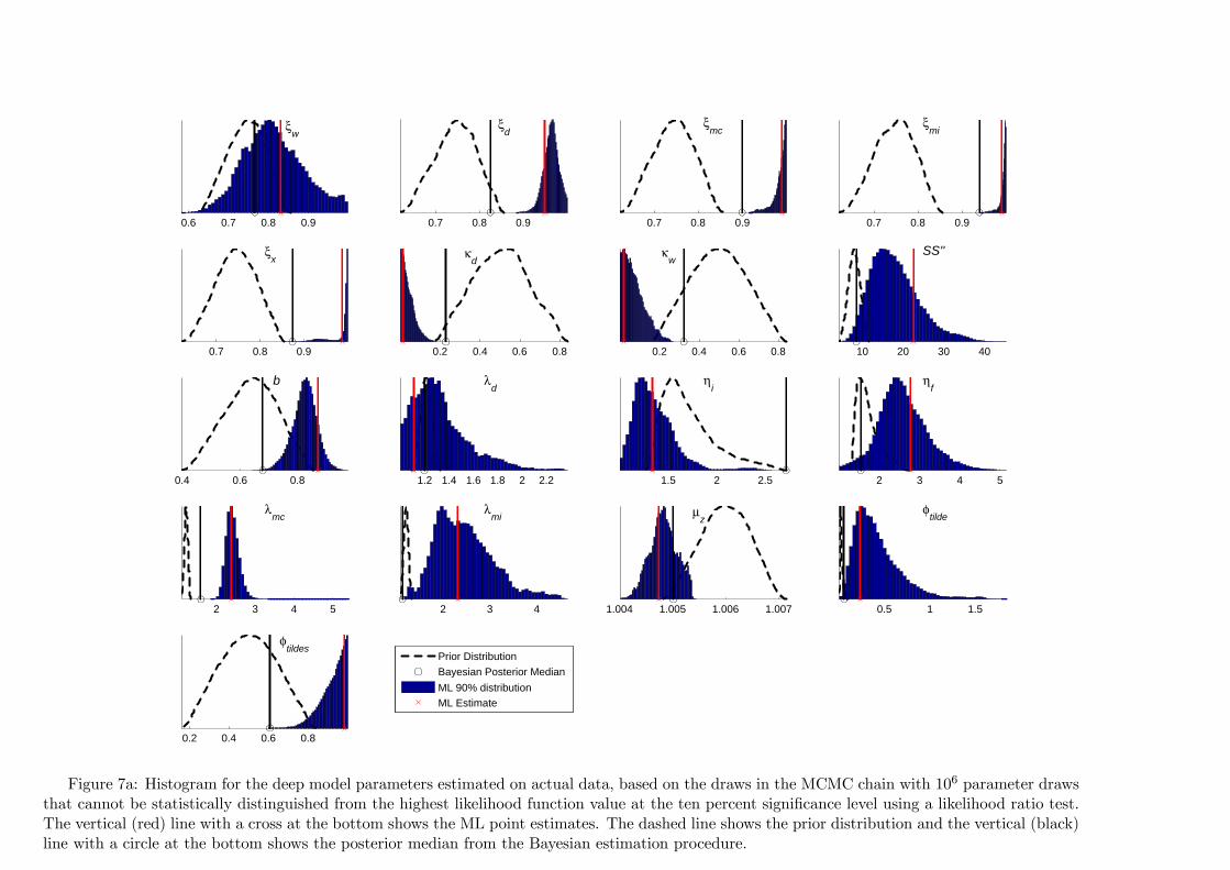
0.6 0.7 0.8 0.9

ξw

0.7 0.8 0.9

ξd

0.7 0.8 0.9

ξmc

0.7 0.8 0.9

ξmi

0.7 0.8 0.9

ξx

0.2 0.4 0.6 0.8

κd

0.2 0.4 0.6 0.8

κw

10 20 30 40

SS''

0.4 0.6 0.8

b

1.2 1.4 1.6 1.8 2 2.2

λd

1.5 2 2.5

ηi

2 3 4 5

ηf

2 3 4 5

λmc

2 3 4

λmi

1.004 1.005 1.006 1.007

μz

0.5 1 1.5

φtilde

0.2 0.4 0.6 0.8

φtildes

Prior DistributionBayesian Posterior MedianML 90% distributionML Estimate

Figure 7a: Histogram for the deep model parameters estimated on actual data, based on the draws in the MCMC chain with 106 parameter drawsthat cannot be statistically distinguished from the highest likelihood function value at the ten percent significance level using a likelihood ratio test.The vertical (red) line with a cross at the bottom shows the ML point estimates. The dashed line shows the prior distribution and the vertical (black)line with a circle at the bottom shows the posterior median from the Bayesian estimation procedure.

0.5 0.6 0.7 0.8 0.9

ρμ

z

0.6 0.7 0.8 0.9

ρε

0.2 0.4 0.6 0.8

ρυ

0.2 0.4 0.6 0.8

ρφ

0.2 0.4 0.6 0.8

ρz

c

0.2 0.4 0.6 0.8

ρz

h

0.2 0.4 0.6 0.8

ρz*

0.5 1 1.5

σz

2 4 6

σε

2 4 6 8

σλ

mc

2 4 6 8

σλ

mi

2 4 6 8

σλ

d

0.5 1 1.5

σϒ

0.5 1 1.5 2 2.5

σφ

0.5 1 1.5

σz

c

2 4 6 8

σz

h

0.5 1 1.5

σz*

2 4 6 8

σλ

x


Figure 7b: Histogram for the shock parameters estimated on actual data, based on the draws in the MCMC chain with 106 parameter draws thatcannot be statistically distinguished from the highest likelihood function value at the ten percent significance level using a likelihood ratio test. Thevertical (red) line with a cross at the bottom shows the ML point estimates. The dashed line shows the prior distribution and the vertical (black)line with a circle at the bottom shows the posterior median from the Bayesian estimation procedure.

0.2 0.4 0.6 0.8 1 1.2

σR

0.1 0.2 0.3 0.4

σπ

bar

0.7 0.75 0.8 0.85 0.9 0.95

ρR

0.1 0.2 0.3 0.4 0.5 0.6

rπ(1- ρ

R)

0 0.1 0.2 0.3 0.4 0.5

rΔπ

-0.03 -0.02 -0.01 0 0.01 0.02

rx(1- ρ

R)

0 0.02 0.04 0.06

ry(1- ρ

R)

-0.1 0 0.1 0.2 0.3 0.4

rΔy


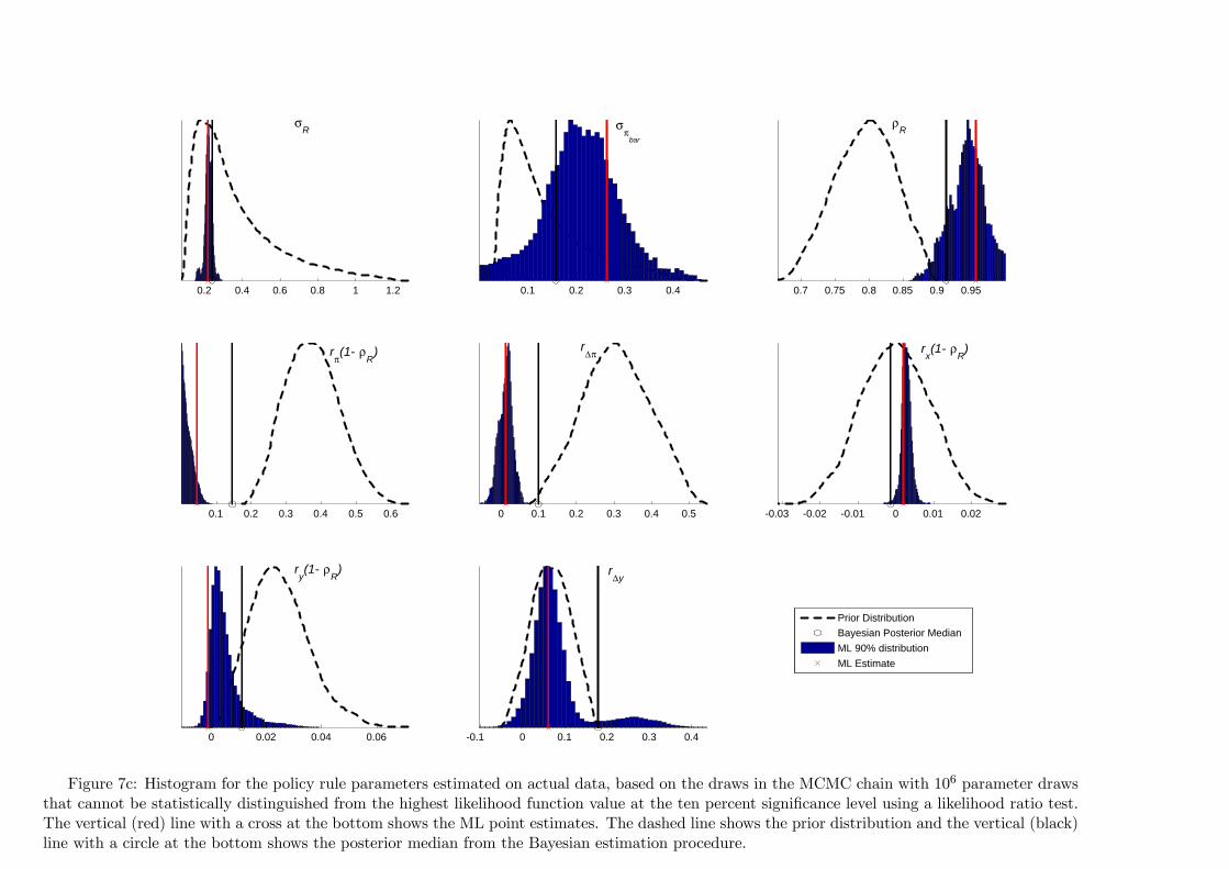
Figure 7c: Histogram for the policy rule parameters estimated on actual data, based on the draws in the MCMC chain with 106 parameter drawsthat cannot be statistically distinguished from the highest likelihood function value at the ten percent significance level using a likelihood ratio test.The vertical (red) line with a cross at the bottom shows the ML point estimates. The dashed line shows the prior distribution and the vertical (black)line with a circle at the bottom shows the posterior median from the Bayesian estimation procedure.

Model misspeci�cation seems important

Statistically signi�cant increase in log-likelihood compared toBayesian estimation

increase from �2128.6 to �2022.2support evidence that model su¤er from misspeci�cationAdolfson et al. (2008), λopt � 7 < ∞DSSW (2007, JBES), λ � 0.5

Degree of price stickiness too high relative to microeconomic evidence

Firm-speci�c capital cannot help this shortcomingCorrelated markup shocks brings down estimated price stickiness

Adolfson et al. (2005), Del Negro and Schorfheide (2008),Smets and Wouters (2007)Need too volatile markup shocks (Chari, Kehoe, McGrattan,2008)Counterfactual implications for �rm pro�ts

Concluding remarks

Parameter identi�cation is possible in DSGE models if likelihoodbased techniques are employed

Weak identi�cation in small samplesSet of observed variables matterPerformance of ML estimator depends on parameterization of theDGP

Results contrast Canova and Sala (2009) and Iskrev (2008, 2009)

Restrictive shock processes (e.g. price markup shocks)Calibrate some parameters (e.g. labor supply elasticity and wagemarkup)

Problems associated with model misspeci�cation

DSSW (2007) and Adolfson et al. (2008)

parameter identi–cation in an estimated new keynesian ... · prior research on identi–cation...

Documents