parameter-less co-clustering for star-structured

HAL Id: hal-00794744https://hal.archives-ouvertes.fr/hal-00794744

Submitted on 26 Feb 2013

HAL is a multi-disciplinary open accessarchive for the deposit and dissemination of sci-entific research documents, whether they are pub-lished or not. The documents may come fromteaching and research institutions in France orabroad, or from public or private research centers.

L’archive ouverte pluridisciplinaire HAL, estdestinée au dépôt et à la diffusion de documentsscientifiques de niveau recherche, publiés ou non,émanant des établissements d’enseignement et derecherche français ou étrangers, des laboratoirespublics ou privés.

Parameter-less co-clustering for star-structuredheterogeneous data

Dino Ienco, Céline Robardet, Ruggero Pensa, Rosa Meo

To cite this version:Dino Ienco, Céline Robardet, Ruggero Pensa, Rosa Meo. Parameter-less co-clustering for star-structured heterogeneous data. Data Mining and Knowledge Discovery, Springer, 2013, 26 (2), pp.217-254. 10.1007/s10618-012-0248-z. hal-00794744

https://hal.archives-ouvertes.fr/hal-00794744

https://hal.archives-ouvertes.fr

Noname manuscript No.(will be inserted by the editor)

Parameter-Less Co-Clustering for Star-Structured

Heterogeneous Data

Dino Ienco · Celine Robardet · RuggeroG. Pensa · Rosa Meo

Received: date / Accepted: date

Abstract The availability of data represented with multiple features comingfrom heterogeneous domains is getting more and more common in real worldapplications. Such data represent objects of a certain type, connected to othertypes of data, the features, so that the overall data schema forms a star struc-ture of inter-relationships. Co-clustering these data involves the specificationof many parameters, such as the number of clusters for the object dimensionand for all the features domains. In this paper we present a novel co-clusteringalgorithm for heterogeneous star-structured data that is parameter-less. Thismeans that it does not require either the number of row clusters or the numberof column clusters for the given feature spaces. Our approach optimizes theGoodman-Kruskal’s τ , a measure for cross-association in contingency tablesthat evaluates the strength of the relationship between two categorical vari-ables. We extend τ to evaluate co-clustering solutions and in particular weapply it in a higher dimensional setting. We propose the algorithm CoStar

which optimizes τ by a local search approach. We assess the performance ofCoStar on publicly available datasets from the textual and image domainsusing objective external criteria. The results show that our approach outper-forms state-of-the-art methods for the co-clustering of heterogeneous data,while it remains computationally efficient.

Dino Ienco1,3 · Celine Robardet2 · Ruggero G. Pensa1 · Rosa Meo1

1Dept. of Computer Science, University of TorinoI-10139 Torino, ItalyE-mail: ienco,[email protected]

2Universite de Lyon, CNRS, INSA-Lyon, LIRIS UMR5205,F-69621 Villeurbanne, FranceE-mail: [email protected]

3IRSTEA Montpellier, UMR TETISF-34093 Montpellier, FranceE-mail: [email protected]

Author-produced version of the article published in Data Mining and Knowledge Discovery, 2013, 26(2), 217-254. The original publication is available at http://www.springer.com DOI : 10.1007/s10618-012-0248-z

ienco,[email protected]

[email protected]

[email protected]

2

1 Introduction

Clustering is by far one of the most popular techniques among researchers andpractitioners interested in the analysis of data from different sources. It is oftenemployed to obtain a first schematic view of what the data looks like, since itdoes not require much background knowledge, usually incorporated into theclass labels, nor involves pre- or post-treatment of the data. Applications ofclustering techniques range over a wide variety of domains, from biology tophysics, from e-commerce to social network analysis. As such, there exists awide literature which investigates new algorithms, measures, and applicationdomains for data clustering.

Usually, data come in the form of a set of objects described by a set ofattributes that can be heterogeneous for type and underlying properties. Forinstance, the most common ones are numeric, categorical, boolean, textual,sequential, or networked. In the most classic settings, objects are representedby features obtained by a unique source of information or view. For instance,census data are produced by a national statistical institute, textual data areextracted from a document repository, tagged items come from a social mediawebsite, and so on.

However, in some cases, computing clusters over a single view is not suf-ficient to capture all the intrinsic similarities or differences between objects.Consider, for instance, an e-commerce website specialized in high-tech prod-ucts, where each product is described by a general description, a technicalnote, and reviews are posted by customers. It is quite common to look forcertain products and be unable to decide because of some incomplete tech-nical details, uninformative descriptions or misleading reviews. The typicalcustomer behavior is then to merge all the different sources of information,by considering them for what they are: technical notes give details on com-ponents and features (usually taken from the producer’s website); general de-scriptions provide synthetic views of the main characteristics and advantagesof the products; customers’ reviews possibly complete missing details and addfurther useful information.

As another example consider a scientific digital library where each paperis described by its textual content (e.g., title, abstract and/or keywords), bythe list of co-authors, and by a list of cited papers. If the goal is, for in-stance, to find the scientific communities interested in the same research field,one can try to apply a clustering algorithm over one of the feature spaces.However, intersections between communities are very common: for instance,people interested in knowledge discovery and data mining may work and pub-lish together with people coming from the information retrieval community.Abstracts or titles on their own are not sufficiently informative: they mightfocus on the applicative aspects of the work, or be too generic or specific. Ci-tations can be misleading as well: in some cases papers refer to other worksdealing with similar topics but in other fields of research; sometimes papersare cited for another purpose than reporting closely related works. Therefore,clustering papers using only one feature space could lead to imprecise results.


3

Instead, taking into account all the feature space may help in identifying moreinteresting and relevant clusters.

A straightforward solution consists in merging all the feature spaces into asingle one, and applying a clustering algorithm on the overall table. Howeverthis solution would not always work as expected, and this for several reasons:first the feature space may contain different types of attributes; second, eventhough the attribute type is homogeneous, each feature may fit a specificmodel, show properties or be affected by certain problems such as noise, whichmight affect in a different form the other feature space. Third, the form of datamay vary significantly from one space to another: document-keyword data aretypically sparse, while categorical data are usually dense. Networked data,such as social networks, contains highly dense portions of nodes, and sparseones. Fourth, even though the spaces do not fall into the above-mentionedcases, their cardinality may vary drastically having the consequence that largerfeature spaces have more influence on the clustering process than smaller ones.

To cope with the limitation of traditional clustering algorithms on mul-tiple views data, a new clustering formulation was introduced in 2004, theso-called multi-view clustering approach [4]. Instead of considering a standardclustering approach over each single-view, the authors proposed an algorithmbased on EM that clusters each view on the basis of the partitions of the otherviews. A strongly related approach is the so-called star-structured high-order

heterogeneous co-clustering [13]. Though it has never been explicitly linkedto multi-view clustering, this family of algorithms addresses the same issuesof a co-clustering approach that simultaneously clusters objects and featuresfrom the different spaces. Co-clustering methods have two main advantages:they are more effective in dealing with the well-known problem of the curseof dimensionality, and they provide an intensional description of the objectclusters by associating a cluster of features to each cluster of objects. Whenapplied on multi-view data, the several views, or feature spaces, as well asthe object set, are simultaneously partitioned. A common problem of existingco-clustering approaches (as well as of other dimensionality reduction tech-niques such as non-negative matrix factorization [21]), is that the number ofclusters/components is a parameter that has to be specified before the execu-tion of the algorithm. Choosing a correct number of clusters is not easy, andmistakes can have undesirable consequences. As mentioned in [19], incorrectparameter settings may cause an algorithm to fail in finding the true patternsand may lead the algorithm to report spurious patterns that do not reallyexist. Existing multi-view co-clustering methods have as many parameters asthere are views in the data, plus one for the partition of objects.

In this paper we propose a new co-clustering formulation for high-orderstar-structured data that automatically determines the number of clusters atrunning time. This is obtained thanks to the employment of a multiobjectivelocal search approach over a set of Goodman-Kruskal’s τ objective functions,that will be introduced in Section 3.1. The local search approach aims atmaximizing these functions, comparing two solutions on the basis of a Pareto-dominance relation over the objective functions. Due to the fact that those


4

functions have a defined upper limit that is independent of the numbers ofclusters, the τ functions can be used to compare co-clusterings of differentsizes. On the contrary, measures that are usually employed in co-clusteringapproaches, like the loss of mutual information [11] or more generally theBregman divergence [2], are optimized for a specific partition, usually the dis-crete one. Moreover, the stochastic local search algorithm we proposed enablesthe adaptation of the number of clusters during the optimization process. Lastbut not least, unlike most of the existing approaches, our algorithm is designedto fit any number of views: when a single feature space is considered, the al-gorithm is equivalent to the co-clustering approach presented in [30].

The remainder of this paper is organized as follows: Section 2 briefly ex-plores the state of the art in star-structured co-clustering and multi-view clus-tering. The theoretic fundamental details are presented in Section 3 whilethe technical issues of our approach are provided in Section 4. In Section 5we present the results of a comprehensive set of experiments on multi-viewhigh-dimensional text and image data, as well as a qualitative evaluation ona specific result and a scalability analysis. Finally, Section 6 concludes.

2 Related Work

Co-clustering has been studied in many different application contexts includ-ing text mining [11], gene expression analysis [8,27] and graph mining [5] wherethese methods have yielded an impressive improvement in performance overtraditional clustering techniques. The methods differ primarily by the criterionthey optimize, such as minimum loss in mutual information [11], sum-squareddistance [8], minimum description length (MDL) [5], Bregman divergence [2]and non-parametric association measures [29,17]. Among these approaches,only those ones based on MDL and association measure are claimed to beparameter-free [19]. However, methods based on MDL are strongly restrictedby the fact they can only handle binary matrices. Association measures, such asGoodman and Kruskal τ , are internal measures of the quality of a co-clusteringbased on statistical considerations. They have also another advantage: they candeal with both binary and counting/frequency data [17,29]. From an algorith-mic point of view, the co-clustering problem has been shown to be NP-hard [1]when the number of row and column clusters are fixed. Therefore, proposedmethods so far are based on heuristic approaches.

Several clustering and co-clustering methods for heterogeneous star-struc-tured data have been proposed recently. Long et al. [23] use spectral clusteringto iteratively embed each type of data objects into low dimensional spaces ina way that takes advantage of the interactions among the different featurespaces. A partitional clustering algorithm like k-means is then employed toobtain the final clustering computed on the transformed spaces. In [24], aparametric probabilistic approach to cluster relational data is proposed. AMonte Carlo simulation method is used to learn the parameters and to assignobjects to clusters. The problem of clustering images described by segments


5

and captions is considered in [3]. The proposed algorithm is based on Markovrandom fields in which some of the nodes are random variables in the combi-natorial problem.

The co-clustering problem on star-structured data was first considered in[13] where Gao et al. propose to adapt the Information Theory co-clusteringapproach [11] to star-structured data. It consists in optimizing a weightedcombination of mutual information evaluated over each feature space, whereweights are chosen based on the supposed reliability/relevance of their correla-tion. Beyond the parameters inherited from the original algorithm, the weightinvolved in the linear combination also has to be fixed by the end-user. Anotherdrawback of this approach is its complexity, that prevents its use on large-scaledatasets. Greco et al. [15] propose a similar approach based on the linear com-bination of mutual information evaluated on each feature space, where theparameter of the linear combination is automatically determined. Ramage etal. [28], propose a generative clustering algorithm based on latent Dirichletallocation to cluster documents using two different sources of information:document text and tags. Each source is modeled by a probability distributionand a weight value is used to weigh one vector space with respect to the other.During the learning step, the algorithm finds the distribution parameters, andmodels documents, words and tags. In addition to the weight parameter, themethod has another drawback: it constrains the number of hidden topics intext and tag sources to be the same, which is a strong assumption on data thatis not always true. Considering the multi-view clustering problem Cleuziou etal. [9] propose to find a consensus between the clusters from different views.Their approach merges information from each view by performing a fusion pro-cess that identifies the agreement between the views and solves the conflicts.To this purpose they formulate the problem using a fuzzy clustering approachand extend fuzzy k-means algorithm by introducing a penalty term. This termaims at reducing the disagreement between any pair of partitions coming fromthe different views. This approach is sensitive to the parameter setting be-cause, apart from the number of clusters, the algorithm requires two otherparameters that may influence the result. [6] can be considered as the firstattempt that performs multi-view co-clustering. The method is an extensionof the Non-Negative Matrix Factorization approach to deal with multi-viewdata. It computes new word-document and document-category matrices byincorporating user provided constraints through simultaneous distance metriclearning and modality selection. This method is shown to be effective, butits formulation is not flexible. In fact, in order to use more than two featurespaces, one needs to reformulate the whole process. Another problem of thisapproach is that the number of clusters for each feature space is given as aparameter. Furthermore, the number of parameters grows with the number offeature spaces.


6

3 Measuring the quality of a co-clustering on star-structured data

In this section, we introduce the association measure optimized within ourco-clustering approach. Originally designed for evaluating the dependence be-tween two categorical variables, the Goodman and Kruskal τ measure can beused to evaluate the quality of a single-view co-clustering. We generalize itsdefinition to a multi-view setting.

3.1 Evaluating the quality of a co-clustering

Association measures are statistical measures that evaluate the strength ofthe link between two or more categorical variables. Considering partitions ofa co-clustering as categorical variables, these measures have been shown to bewell adapted to determine co-clustering with high quality [29]. Goodman andKruskal τ measure [14] is one of them that estimates the association betweentwo categorical variables X and Y by the proportional reduction of the errorin predicting X knowing or not the variable Y :

τX|Y =eX − E[eX|Y ]

eX

Let say that variable X has m categories X1, · · · , Xm with probabilitiesp1, · · · , pm, variable Y has n categories Y1, · · · , Yn with probabilities q1, · · · , qnand their joint probabilities are denoted rij , for i = 1 · · ·m and j = 1 · · ·n. Theerror in predicting X can be evaluated by eX =

∑m

i=1 pi(1−pi) = 1−∑m

i=1 p2i .

This is the probability that two independent observations from the marginaldistribution of X fall in different categories. The error is minimum (equals to0) when every pi’s is 0 or 1. The error is maximum when pi = 1

mfor all i.

E[eX|Y ] is the expectation of the conditional error taken with respect to thedistribution of Y :

E[eX|Y ] =n∑

j

qj eX|Yj=

n∑

j

qj

m∑

i

rijqj

(1−rijqj

) = 1−m∑

i

n∑

j

r2ijqj

The Goodman-Kruskal’s τX|Y association measure is then equal to:

τX|Y =

∑

i

∑

j

r2ijqj

−∑

i p2i

1−∑

i p2i

(1)

Similarly, the proportional reduction of the error in predicting Y while Xis known is given by:

τY |X =eY − E[eY |X ]

eY=

∑

i

∑

j

r2ijpi

−∑

j q2j

1−∑

j q2j

(2)

Let’s now describe how this association measure can be employed to quan-tify the goodness of a co-clustering. Let O be a set of objects and F a set of


7

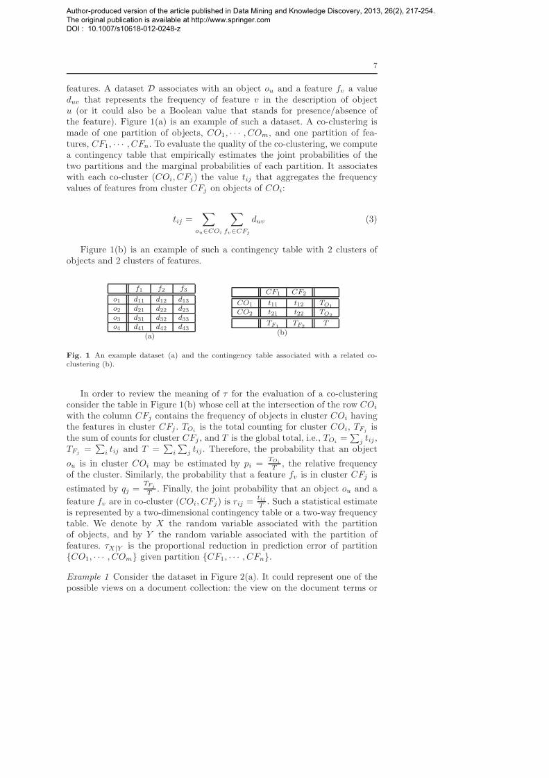
features. A dataset D associates with an object ou and a feature fv a valueduv that represents the frequency of feature v in the description of objectu (or it could also be a Boolean value that stands for presence/absence ofthe feature). Figure 1(a) is an example of such a dataset. A co-clustering ismade of one partition of objects, CO1, · · · , COm, and one partition of fea-tures, CF1, · · · , CFn. To evaluate the quality of the co-clustering, we computea contingency table that empirically estimates the joint probabilities of thetwo partitions and the marginal probabilities of each partition. It associateswith each co-cluster (COi, CFj) the value tij that aggregates the frequencyvalues of features from cluster CFj on objects of COi:

tij =∑

ou∈COi

∑

fv∈CFj

duv (3)

Figure 1(b) is an example of such a contingency table with 2 clusters ofobjects and 2 clusters of features.

f1 f2 f3

o1 d11 d12 d13o2 d21 d22 d23o3 d31 d32 d33o4 d41 d42 d43

(a)

CF1 CF2

CO1 t11 t12 TO1

CO2 t21 t22 TO2

TF1TF2

T

(b)

Fig. 1 An example dataset (a) and the contingency table associated with a related co-clustering (b).

In order to review the meaning of τ for the evaluation of a co-clusteringconsider the table in Figure 1(b) whose cell at the intersection of the row COi

with the column CFj contains the frequency of objects in cluster COi havingthe features in cluster CFj . TOi

is the total counting for cluster COi, TFjis

the sum of counts for cluster CFj , and T is the global total, i.e., TOi=∑

j tij ,TFj

=∑

i tij and T =∑

i

∑

j tij . Therefore, the probability that an object

ou is in cluster COi may be estimated by pi =TOi

T, the relative frequency

of the cluster. Similarly, the probability that a feature fv is in cluster CFj is

estimated by qj =TFj

T. Finally, the joint probability that an object ou and a

feature fv are in co-cluster (COi, CFj) is rij =tijT. Such a statistical estimate

is represented by a two-dimensional contingency table or a two-way frequencytable. We denote by X the random variable associated with the partitionof objects, and by Y the random variable associated with the partition offeatures. τX|Y is the proportional reduction in prediction error of partitionCO1, · · · , COm given partition CF1, · · · , CFn.

Example 1 Consider the dataset in Figure 2(a). It could represent one of thepossible views on a document collection: the view on the document terms or


8

the view on the document tags that users adopted to annotate documents in asocial network. Suppose the view is on the terms contained in the documents:each value in the matrix represents the number of occurrences of a specificword (indicated by the matrix column) in a specific document (indicated bythe matrix row). We take into account two possible co-clusterings for thisdataset:

C1 = o1, o2, o3, o4, o5, f1, f2, f3, f4

and C2 = o1, o2, o3, o4, o5, f1, f2, f3, f4

Tables in Figure 2(b) and 2(c) represent the contingency tables for the firstand second co-clustering respectively. The Goodman-Kruskal τX|Y and τY |X

for the first co-clustering are:

τX|Y = τY |X = 0.5937

and for the second one are:

τX|Y = 0.2158 and τY |X = 0.3375

We can observe that the first co-clustering better associates clusters of ob-jects with clusters of features than the second one. In the first co-clustering,objects of CO1 have mostly features of cluster CF1, whereas objects of CO2

are characterized by features of CF2. In the second example, given an objecthaving high frequency values on features of CF1, it is difficult to predict if itbelongs to CO1 or CO2. The τ measure corroborates these facts and in fact ithas higher values for the first co-clustering.

f1 f2 f3 f4

o1 3 4 1 1o2 5 3 0 2o3 6 4 1 0o4 0 1 7 7o5 1 0 6 8

(a)

CF1 CF2

CO1 25 5 30CO2 2 28 30

27 33 60

(b)

CF1 CF2

CO1 15 4 19CO2 12 29 41

27 33 60

(c)

Fig. 2 An example dataset (a) and the contingency tables that correspond to C1 (b) andC2 (c).

Analyzing the properties of τ , we can observe that it satisfies many desir-able properties of a co-clustering measure. First, it is invariant by rows and


9

columns permutation. Second, it takes values between [0, 1]: (1) τX|Y is 0 iffknowledge of Y classification is of no help in predicting the X classification,i.e. there is independence between the object and feature clusters; (2) τX|Y is 1iff knowledge of an individual’s Y cluster completely specifies his X class, i.e.each row of the contingency table contains at most one non zero cell. Third,it has an operational meaning: given an object, it is the relative reduction inthe prediction error of the object’s cluster given the partition of features, in away that preserves the category distribution [14]. Finally, unlike many otherassociation measures such as χ2, τ has a defined upper limit that is indepen-dent of the numbers of classes m and n. Therefore, τ can be used to compareco-clusterings of different sizes.

3.2 The star schema

In the context of high-order star-structured co-clustering, the same set of ob-jects is represented in different feature spaces. Such data represent objects of acertain type, connected to other types of data, the features, so that the overalldata schema forms a star structure of inter-relationships. The co-clusteringtask consists in clustering simultaneously the set of objects and the set ofvalues in the different feature spaces. In this way we obtain a partition ofthe objects influenced by each of the feature spaces and at the same time apartition of each feature space. Considering N feature spaces that have to beclustered, in this paper we study a way to extend the τ measure to performco-clustering of the data when the number of the involved dimensions is high.

In Figure 3 we show an example of a star-structured data schema. Theset of objects is shown at the center of the star. For example it could be aset of documents. The set of objects is then described with multiple views bymore features (Feature1, Feature2, Feature3). For instance, Feature1 could bethe set of the vocabulary words and the values d1ij represent the number of

occurrences of the word f1j in the document Oi; Feature2 could be the set oftags adopted by the users of a social community in their annotations and thevalues d2ij represent the number of users that used the tag f2j in the documentOi; Feature3 could be the set of authors who cited documents in the givenset and the feature values represent the number of citations. For the completedescription of each object we have to make reference to the different featurespaces. The values of each feature have their own distributions in the documentset and are described by the different contingency tables. At this point boththe document set and the feature spaces might be partitioned into co-clusterswhere all the dimensions contribute to determine the partitions.

3.3 Evaluating the quality of a star-structured co-clustering

Evaluating the quality of the partition of objects, given the partitions of fea-tures, is formalized as follows. The partition of objects is associated with the


10

Objects

O1

O2

...

OM

f11 f12 . . . f1n1

O1 d111 d1

12 . . . . . .

O2 d121

. .

. .

. .

OM d1M1 . . . . . . d1

Mn1

Feature 1

f31 f32 . . . f3n3

O1 d311 d3

12 . . . . . .

O2 d321

. .

. .

. .

OM d3M1 . . . . . . d3

Mn3

Feature 3

f21 f22 . . . f2n2

O1 d211 d2

12 . . . . . .

O2 d221

. .

. .

. .

OM d2M1 . . . . . . d2

Mn2

Feature 2

Fig. 3 The data star-schema.

dependent variable X , and the N partitions of the feature spaces are consid-ered as many independent variables Y = Y 1, . . . , Y N. Each variable Y k ∈ Yhas nk categories Y k

1 , · · · , Y knk

with probabilities qk1 , . . . , qknk

and X has m cate-

gories X1, · · · , Xm. However, for each variable Y k, the m categories of X havedifferent probabilities pk1 , · · · , p

km, k = 1 · · ·N . The joint probabilities between

X and any Y k ∈ Y are denoted by rkij , for i = 1 · · ·m and j = 1 · · ·nk. Theerror in predicting X is the sum of the errors over the independent variablesof Y: eX =

∑Nk=1

∑mi=1 p

ki (1 − pki ) = N −

∑Nk=1

∑mi=1(p

ki )

2. E[eX|Y ] is theexpectation of the conditional error taken with respect to the distributions ofall Y k ∈ Y:

E[eX|Y ] =N∑

k

nk∑

j

qkj eX|Y kj=

N∑

k

nk∑

j

qkj

m∑

i

rkijqkj

(1−rkijqkj

) = N−N∑

k

m∑

i

nk

∑

j

(rkij)2

qkj

The generalized Goodman-Kruskal’s τX|Y association measure is then equalto:

τX|Y =

∑

k

∑

i

∑

j

(rkij)2

qkj−∑

k

∑

i(pki )

2

N −∑

k

∑

i(pki )

2(4)

If we consider Y k as a dependent variable, and X as an independent variable,the corresponding τY k|X is computed as described in the previous section (see


11

equation (2)), i.e.:

τY k|X =eY k − E[eY k|X ]

eY k

=

∑

i

∑

j

(rkij)2

pki

−∑

j(qkj )

2

1−∑

j(qkj )

2(5)

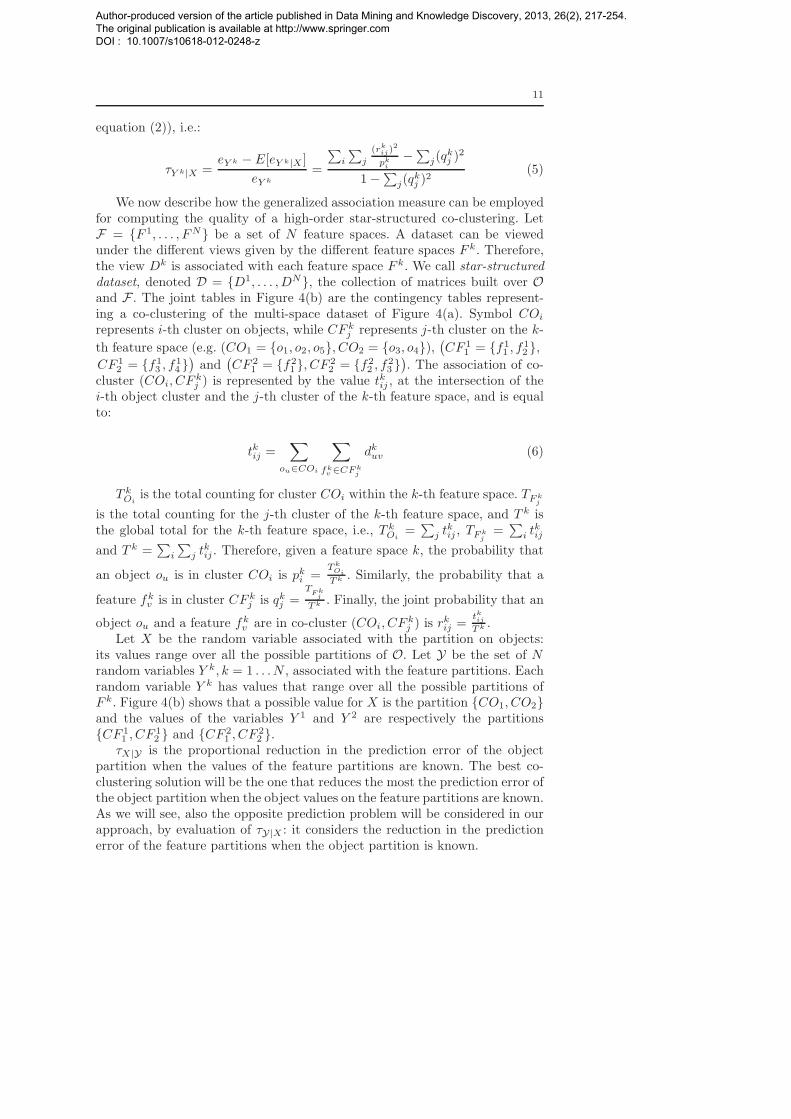
We now describe how the generalized association measure can be employedfor computing the quality of a high-order star-structured co-clustering. LetF = F 1, . . . , FN be a set of N feature spaces. A dataset can be viewedunder the different views given by the different feature spaces F k. Therefore,the view Dk is associated with each feature space F k. We call star-structureddataset, denoted D = D1, . . . , DN, the collection of matrices built over Oand F . The joint tables in Figure 4(b) are the contingency tables represent-ing a co-clustering of the multi-space dataset of Figure 4(a). Symbol COi

represents i-th cluster on objects, while CF kj represents j-th cluster on the k-

th feature space (e.g. (CO1 = o1, o2, o5, CO2 = o3, o4),(

CF 11 = f1

1 , f12 ,

CF 12 = f1

3 , f14 )

and(

CF 21 = f2

1, CF 22 = f2

2 , f23 )

. The association of co-cluster (COi, CF k

j ) is represented by the value tkij , at the intersection of thei-th object cluster and the j-th cluster of the k-th feature space, and is equalto:

tkij =∑

ou∈COi

∑

fkv ∈CFk

j

dkuv (6)

T kOi

is the total counting for cluster COi within the k-th feature space. TFkj

is the total counting for the j-th cluster of the k-th feature space, and T k isthe global total for the k-th feature space, i.e., T k

Oi=∑

j tkij , TFk

j=∑

i tkij

and T k =∑

i

∑

j tkij . Therefore, given a feature space k, the probability that

an object ou is in cluster COi is pki =TkOi

Tk . Similarly, the probability that a

feature fkv is in cluster CF k

j is qkj =TFkj

Tk . Finally, the joint probability that an

object ou and a feature fkv are in co-cluster (COi, CF k

j ) is rkij =

tkijTk .

Let X be the random variable associated with the partition on objects:its values range over all the possible partitions of O. Let Y be the set of Nrandom variables Y k, k = 1 . . .N , associated with the feature partitions. Eachrandom variable Y k has values that range over all the possible partitions ofF k. Figure 4(b) shows that a possible value for X is the partition CO1, CO2and the values of the variables Y 1 and Y 2 are respectively the partitionsCF 1

1 , CF 12 and CF 2

1 , CF 22 .

τX|Y is the proportional reduction in the prediction error of the objectpartition when the values of the feature partitions are known. The best co-clustering solution will be the one that reduces the most the prediction error ofthe object partition when the object values on the feature partitions are known.As we will see, also the opposite prediction problem will be considered in ourapproach, by evaluation of τY|X : it considers the reduction in the predictionerror of the feature partitions when the object partition is known.


12

f11

f12

f13

f14

f21

f22

f23

o1 d111

d112

d113

d114

d211

d212

d213

o2 d121

d122

d123

d124

d221

d222

d223

o3 d131

d132

d133

d134

d231

d232

d233

o4 d141

d142

d143

d144

d241

d242

d243

o5 d151 d152 d153 d154 d251 d252 d253(a)

CF 11 CF 1

2 CF 21 CF 2

2

CO1 t111

t112

T 1O1

t211

t212

T 2O1

CO2 t121

t122

T 1O2

t221

t222

T 2O2

TF11

TF12

T 1 TF21

TF22

T 2

(b)

Fig. 4 An example of a star-structured dataset (a) and the contingency table associatedwith a related star-structured co-clustering (b).

Example 2 Example in Figure 4(a) has been instantiated in the dataset ofFigure 5(a): it could represent a collection of documents. Suppose the firstfeature space is the space of the terms occurring in the documents, while thesecond feature space is the space of the tags associated by the users of a socialnetwork. Each counting in the first feature space (f1

1 · · · f14 ) represents, for

instance, the occurrences of a specific word in a specific document, while thecounting in the second feature space (f2

1 · · · f23 ) are the number of users who

associated a specific tag with a specific document. We take into account twopossible co-clusterings for this dataset:

C1 = CO1 = o1, o2, o3, CO2 = o4, o5 ×

CF 11 = f1

1 , f12 , CF 1

2 = f13 , f

14 ∪ CF 2

1 = f21 , CF 2

2 = f22 , f

23

C2 = CO3 = o1, o3, o5, CO4 = o2, o4 ×

CF 13 = f1

1 , f13 , CF 1

4 = f12 , f

14 ∪ CF 2

1 = f21 , CF 2

2 = f22 , f

23

Tables in Figure 5(b) and 5(c) represent the contingency tables for C1 and C2

respectively. For the first co-clustering, the Goodman-Kruskal τX|Y and τY k|X

measures are:

τX|Y = 0.6390, τY 1|X = 0.5937, τY 2|X = 0.6890

τ values have been computed respectively on the contingency tables:

CO1, CO2 × CF 11 , CF 1

2 , CF 21 , CF 2

2

CF 11 , CF 1

2 × CO1, CO2

CF 21 , CF 2

2 × CO1, CO2

For the second co-clustering, they are:

τX|Y = 0.0119, τY 1|X = 0.0234, τY 2|X = 0.0008

Since all the three τ values for the first co-clustering are greater than thesecond ones, we can conclude that the first co-clustering better captures theinteractions between objects and features of each space.


13

f11

f12

f13

f14

f21

f22

f23

o1 3 4 1 1 0 8 5o2 5 3 0 2 0 6 9o3 6 4 1 0 2 2 2o4 0 1 7 7 9 1 0o5 1 0 6 8 7 0 1

(a)

CF 11

CF 12

CF 21

CF 22

CO1 25 5 30 2 32 34CO2 2 28 30 16 2 18

27 33 60 18 34 52

(b)

CF 11

CF 12

CF 21

CF 22

CO1 18 17 35 9 18 27CO2 12 13 25 9 16 25

30 30 60 18 34 52

(c)

Fig. 5 An example dataset (a) and two contingency tables associated with the star-structured co-clusterings C1 (b) and C2 (c).

4 A stochastic local search approach for high-order star-structuredco-clustering

We formulate our co-clustering approach for star-structured data asa multi-objective combinatorial optimization problem [18] which aimsat optimizing N + 1 objective functions based on Goodman-Kruskal’sτ measure. Given a star-structured dataset D over O and F , the goalof the star-structured data co-clustering is to find a set of partitionsY = Y 1, . . . , Y k, . . . , Y N over the feature set F = F 1, . . . , F k, . . . , FN,and a partition X of the object set O such that

maxY∪X∈P

τ(Y ∪X) =(

τY 1|X , . . . , τY k|X , . . . , τY N |X , τX|Y

)

(7)

where P is the discrete set of candidate partitions and τ is a function fromP to Z, where Z = [0, 1]N+1 is the set of vectors in the objective space,i.e., zi = τY i|X (see equation (5)), ∀i = 1, . . . , N and zN+1 = τX|Y (seeequation (4)).

To compare different candidate partitions of P , one can either use ascalarization function, that maps Z into R (such as the weighted sum), orone can employ a dominance-based approach, that induces a partial orderover P . As for combinatorial problem there may exist many truly optimalpartitions that are not optimal for any weighted sum scalarization function[22], we consider in the following a Pareto-dominance approach. The goalis to identify optimal partitions Popt ⊂ P , where optimality consists in thefact that no solution in P \Popt is superior to any solution of Popt on every


14

objective function. This set of solutions is known as Pareto optimal set ornon-dominated set. These concepts are formally defined below.

Definition 1 (Pareto-dominance) An objective vector z ∈ Z is said todominate an objective vector z′ ∈ Z iff ∀i ∈ 1, . . . , N + 1, zi ≥ z′i and∃j ∈ 1, . . . , N + 1, such that zj > z′j . This relation is denoted z ≻ z′

hereafter.

Definition 2 (Non-dominated objective vector and Pareto opti-mal solution) An objective vector z ∈ Z is said to be non-dominated iffthere does not exist another objective vector z′ ∈ Z such that z′ ≻ z.

A solution p ∈ P is said to be Pareto optimal iff its mapping in theobjective space (τ(p)) results in a non-dominated vector.

Thus, the star-structured data co-clustering problem is to seek for aPareto optimal solution of equation (7). As this problem is more difficultthan the co-clustering problem with fixed numbers of object and featureclusters, which is known to be NP-hard [1], we propose, in subsection 4.1,a Stochastic Local Search algorithm CoStar to solve it. This algorithmsearches for a near optimal solution given a local knowledge provided bythe definition of a neighborhood [25]. We demonstrate, in subsection 4.2,that CoStar outputs a Pareto local optimum solution of the problem. Insubsection 4.3, we propose a way to evaluate a neighbor solution incremen-tally. Finally subsection 4.4 gives the overall complexity of CoStar and ofits competitors.

4.1 Multiple feature space co-clustering algorithm

We build our algorithm on the basis of τCoClust [30], whose goal is to finda partition X of objects and a partition Y of features such that Goodman-Kruskal’s τX|Y and τY |X are maximized. The algorithm locally optimizesthe two coefficients by updating step by step the partitions. The basic up-dating procedure consists in running through the neighborhood of eachpartition and choose the partition that increases the most the measures.This neighborhood is made of partitions where a peculiar element is movedfrom one cluster to another. Let us first consider the improvement of par-tition X . After randomly picking up a cluster and randomly picking upan object in that cluster, the procedure assigns this object to the cluster(possibly an empty one) that mostly increases τX|Y . In a following phase, itconsiders the improvement of the features partition Y : it randomly picks upa feature from a randomly obtained cluster and assigns this feature to thecluster that mostly increases τY |X . Starting from the discrete partitions, thealgorithm alternatively updates the partitions X and Y until a convergencecriterion is satisfied. Unlike other co-clustering approaches, that require thenumber of co-clusters as parameter, τCoClust is able to automatically de-termine the most appropriate numbers of clusters for X and Y . This is due


15

to two characteristics: (1) the τ coefficient has a defined upper limit that isindependent of the numbers of clusters (while other measures, such as theloss in mutual information [11] have not) and thus enables comparison ofco-clusterings of different sizes, and (2) the updating procedure can createor delete clusters at any time during the iterative process.

Let us now present algorithm CoStar as an extension of τCoClustalgorithm to multi-view co-clustering. CoStar is shown in Algorithm 1.It takes in input the dataset D and alternatively optimizes the partitionof the objects, working on the random variable X , and each partition overeach feature set F k, working on the random variables Y k, until a numberof iterations Niter is reached.

Algorithm 1 CoStar(D,Niter)

1: Initialize Y 1, · · · , Y N , X with discrete partitions2: i← 03: T ← ∅4: for k = 1 to N do

5: T k ← ContingencyTable(X,Y k,Dk)6: T ← T

⋃T k

7: end for

8: while (i ≤ Niter) do

9: [X,T ]← OptimizeMultiObjectCluster(X, Y , T )10: for k = 1 to N do

11: [Y k, T k]← OptimizeFeatureCluster(X, Y k, T k)12: end for

13: i← i+ 114: end while

15: return Y 1, · · · , Y N ,X

CoStar first initializes the partitions Y 1, · · · , Y N and X with discretepartitions (that is, partitions with a single element per cluster) and thencomputes the contingency tables T k between the partition X and alter-natively each partition Y k over the feature set F k. The function Con-

tingencyTable computes equation (6) (initialization step at lines 4-7).Then, from line 8 to 14, it performs a stochastic local search method by al-ternatively optimizing partition X (line 9) and each partition Y k (line 11).The candidate partitions considered by the local search algorithm belongto the neighborhood of Y ∪ X as defined in equation (8) page 19. Func-tion OptimizeMultiObjectCluster substitutes the object partition Xfor the partition in the neighborhood of X that mostly increases τX|Y (see

Algorithm 2). This measure takes into account all the partitions Y k ∈ Yand their associated contingency tables T =

⋃

k Tk. Function Optimize-

FeatureCluster substitutes the feature partition Y k for the partitionin the neighborhood of Y k that mostly increases τY k|X (see Algorithm 4).These operations are alternated and repeated until a stopping condition issatisfied. This condition can be based on a convergence criterion of τ , but,


16

for simplicity, we bound the number of iterations by Niter in the currentversion of the algorithm.

Algorithm 2 OptimizeMultiObjectCluster(X,Y, T )1: Randomly choose a cluster xb ∈ X

2: Randomly choose an object o ∈ xb

3: ND ← xb4: maxτX|Y

← τX|Y (T )

5: for all xe ∈ X ∪ ∅ s.t. xb 6= xe do

6: [X′, T ′]← Update(X, T, o, xb, xe)7: if (τX′|Y(T ′) > maxτX|Y

) then

8: maxτX|Y← τX′|Y(T ′)

9: ND ← xe10: else

11: if (τX′|Y (T ′) = maxτX|Y) then

12: ND ← ND ∪ xe13: end if

14: end if

15: end for

16: maxX ,maxT ← FindParetoLocalOptimumObject(ND,X, T, xb, o)17: return maxX ,maxT

Algorithm 3 FindParetoLocalOptimumObject(ND, X, T, xb, o)

1: while Card(ND) > 1 do

2: Take xi, xj ∈ ND s.t. xi 6= xj

3: nb+xi← 0

4: nb+xj← 0

5: [Xi, Ti]← Update(X, T, o, xb, xi)6: [Xj , Tj ]← Update(X, T, o, xb, xj)7: for k = 1 to N do

8: if (τY k|Xi(Ti) > τY k|Xj

(Tj)) then

9: nb+xi← nb+xi

+ 110: else

11: if (τY k|Xi(Ti) < τY k|Xj

(Tj)) then

12: nb+xj← nb+xj

+ 113: end if

14: end if

15: end for

16: if nb+xi≥ nb+xj

then

17: ND ← ND \ xj18: else

19: ND ← ND \ xi20: end if

21: end while

22: return [Xi, Ti]← Update(X,T, o, xb, xi), with xi ∈ ND


17

The stochastic local optimization of the partition X works as follows(see Algorithm 2). The algorithm starts by randomly picking up a clusterxb of X and an element o of xb (lines 1 and 2). Then, all the partitions ofthe neighborhood of X , constituted by the partitions where o is moved toanother cluster of X (possibly the empty one), are considered. To retrievethe partition maxX that increases at most τX|Y among the partitions inthe neighborhood of X and that is not dominated by any partition of thisneighborhood, the algorithm uses a queue, ND, that gathers the possi-bly non-dominated partitions of this neighborhood. Each partition of theneighborhood of X is identified by the cluster to which o belongs. Thus,the queue ND is initialized with xb that represents the partition X (line3). maxτX|Y

is initialized with the current τX|Y value. The loop from line5 to 15 considers all the neighboring partitions of X (xe being the clusterwhere o is moved to, xe ∈ X ∪∅). The function Update (line 6) is called tomodify the contingency tables T =

⋃

k Tk and the partition X with respect

to the new cluster of o. To perform this step, it first moves the elemento from the cluster xb to cluster xe and then performs one or more of thefollowing three actions:

1. if cluster xb is empty after removing o, it deletes cluster xb and updatesthe contingency tables T ′ consequently;

2. if cluster xe is the empty cluster, it adds a new cluster to the partitionand updates the contingency tables T ′ consequently;

3. if the two above mentioned cases do not apply, it simply updates thecontent of T ′ by modifying xb and xe rows.

Each modification of T ′ consists actually in modifying the N contingencytables T k, k = 1, . . . , N .

From line 7 to 14, potentially non-dominated partitions of the neigh-borhood of X are stored in ND. τX′|Y is evaluated using the contingencytables T ′. If it is strictly greater than maxτX|Y

then, given a partition ofND, either X ′ dominates it or neither of the partitions dominates the other(see proof of theorem 1 page 19). Therefore, ND and maxτX|Y

are reinitial-ized respectively with X ′ and τX′|Y . If τX′|Y is equal to maxτX|Y

then xe

is added to the queue ND. Considering X ′ and any partition X of ND, allthe Pareto dominance relation may exist between these two partitions: X ′

may dominate X , X ′ may be dominated by X or neither may dominate theother. Therefore, a partition that is not dominated by any partition of NDwill be identified by the function FindParetoLocalOptimumObject.

When all the neighborhood has been explored, the function FindPare-

toLocalOptimumObject (see Algorithm 3) is called. It processes thequeue ND in order to retrieve a partition non dominated by any other par-tition of ND. To that end, the function compares two partitions Xi and Xj

of ND by counting in nb+xithe number of times τY k|Xi

is strictly greaterthan τY k|Xj

, and in nb+xjthe number of times τY k|Xj

is strictly greater than

τY k|Xi, for k = 1, . . . , N . If nb+xi

≥ nb+xjthen Xj is either dominated by Xi

or neither Xi nor Xj dominate the other (see proof of theorem 1). Thus,


18

the function removes Xj from ND and continues until there is only onepartition in ND.

Algorithm 4 OptimizeFeatureCluster(X,Y k, T k)

1: Randomly choose a cluster yb ∈ Y k

2: Randomly choose a feature f ∈ yb3: ND ← yb4: maxτ

Y k|X← τY k|X(T k)

5: for all ye ∈ Y k ∪ ∅ s.t. yb 6= ye do

6: [Y k′, T k′]← Update(Y k, T k, f, yb, ye)7: if (τY k′|X(T k′) > maxτ

Y k|X) then

8: maxτY k|X

← τY k′|X(T k′)

9: ND ← ye10: else

11: if (τY k′|X(T k′) = maxτY k|X

) then

12: ND ← ND ∪ ye13: end if

14: end if

15: end for

16: maxY k ,maxTk ← FindParetoLocalOptimumFeature(ND, Y k, T k, yb, f)17: return maxY k ,maxTk

Algorithms 4 and 5 optimize partition Y k and work in a similar way thanAlgorithms 2 and 3. However, it is simpler because (1) modifying partitionY k only impacts the contingency table T k′, and (2), in Algorithm 5, thecomparison of two partitions of the queue ND is only done on the basis ofτX|Y value, the others measures (τY k|X , k = 1, . . .N) being equal.

4.2 Local convergence of CoStar

Considering iterated local search algorithms for multi-objective optimiza-tion requires to extend the usual definitions of local optimum to that con-text [26]. Let N : P → 2P be a neighborhood structure that associates toevery solution p ∈ P a set of neighboring solutions N (p) ⊆ P . We define aPareto local optimum with respect to N as follows.

Definition 3 (Pareto local optimum) A solution p ∈ P is a Paretolocal optimum with respect to the set of solutions N (p) that constitutes theneighborhood of p, if and only if there is no r ∈ N (p) such that τ(r) ≻ τ(p)(see equation (7)).

In algorithm CoStar, the neighborhood function is defined as follows.Let p = Y ∪X be an element of P . W i denotes either the partition Y i, ifi ∈ 1, . . . , N, or the partition X , if i = N + 1. Let wb be a cluster of W i

and let u be an element of wb. The neighborhood N of p is determined by


19

Algorithm 5 FindParetoLocalOptimumFeature(ND, Y k, T k, yb, f)

1: while Card(ND) > 1 do

2: Take yi, yj ∈ ND s.t. yi 6= yj

3: nb+yi ← 0

4: nb+yj ← 0

5: [Y ki , T k

i ]← Update(Y k, T k, f, yb, yi)

6: [Xkj , T

kj ]← Update(Y k, T k, f, yb, yj)

7: Yi ← Y \ Y k ∪ Y ki

8: Yj ← Y \ Y k ∪ Y kj

9: if (τX|Yi(T k

i ) > τX|Yj(T k

j )) then

10: nb+yi ← nb+yi + 111: else

12: if (τX|Yi(T k

i ) < τX|Yj(T k

j )) then

13: nb+yj ← nb+yj + 114: end if

15: end if

16: if nb+yi ≥ nb+yj then

17: ND ← ND \ yj18: else

19: ND ← ND \ yi20: end if

21: end while

22: return [Y ki , T k

i ]← Update(Y k, T k, f, yb, yi), with yi ∈ ND

the movement of the element u from the cluster wb to the cluster we in W i.It is given by the substitution in p of W i by W i′:

N(i,wb,u)(Y ∪X) = Y ∪X \W i ∪W i′ (8)

with W i′ = W i \ wb \ we ∪ wb \ u ∪ we ∪ u and we ∈ W i ∪ ∅.

Theorem 1 The iterated local search algorithm CoStar terminates in a

finite number of steps and outputs a Pareto local optimum with respect to

N(i,wb,u).

Proof We consider a partition W i ∈ Y ∪X. Algorithm CoStar (in func-tions OptimizeMultiObjectCluster and OptimizeFeatureClus-

ter) randomly picks-up a cluster wb from partition W i and an element u ∈wb. Then, it systematically explores the neighborhood N(i,wb,u)(Y∪X) andretrieves the set of the corresponding neighboring solutions (co-clustering)ND defined by:

ND = s ∈ N(i,wb,u)(Y ∪X) | ∀t ∈ N(i,wb,u)(Y ∪X), zi(s) ≥ zi(t)

Considering a solution s ∈ ND and a solution r ∈ N(i,wb,u)(Y ∪X), wehave zi(s) ≥ zi(r) and the following situations can occur:

1. If zi(s) > zi(r) and ∀k ∈ 1, . . . , N + 1, k 6= i, zk(s) ≥ zk(r), then sdominates r: s ≻ r.


20

2. If zi(s) > zi(r) and ∃k ∈ 1, · · · , N +1, k 6= i, such that zk(s) < zk(r),then, from Definition 1, s 6≻ r and r 6≻ s.

In both cases 1 and 2, r does not belong to ND since zi(s) >zi(r) (see functions OptimizeMultiObjectCluster or Optimize-

FeatureCluster from lines 7 to 9) and s is a Pareto local optimumwith respect to r.

3. If zi(s) = zi(r) and ∀k ∈ 1, · · · , N + 1, k 6= i, zk(s) ≥ zk(r), then,either s is equivalent to r (z(s) = z(r)) or s dominates r: s r.

Therefore, s is a Pareto local optimum with respect to r. From Algo-rithms OptimizeMultiObjectCluster or OptimizeFeatureClus-

ter, both r and s belong to ND. When partitions r and s are com-pared in Algorithms FindParetoLocalOptimumObject or Find-

ParetoLocalOptimumFeature, nb+s ≥ nb+r and the algorithmsdelete r from ND.

4. If zi(s) = zi(r) and ∃k ∈ 1, · · · , N + 1, k 6= i, such that zk(s) < zk(r)and ∃ℓ ∈ 1, · · · , N + 1, ℓ 6= i 6= k, such that zℓ(s) > zℓ(r), then s 6≻ rand r 6≻ s.

Both partitions r and s are non-dominated from each other andare Pareto local optima. They both belong to ND, and AlgorithmsFindParetoLocalOptimumObject or FindParetoLocalOpti-

mumFeature will remove the partition that is strictly greater thanthe other on the smallest number of objective functions zk.

5. If zi(s) = zi(r) and ∀k ∈ 1, · · · , N + 1, zk(s) ≤ zk(r), and ∃ℓ ∈1, · · · , N + 1, ℓ 6= i, such that zℓ(s) < zℓ(r), then r ≻ s.

Therefore, r is a Pareto local optimum with respect to s. Both s and rbelong to ND and Algorithms FindParetoLocalOptimumObject

or FindParetoLocalOptimumFeature will identify that s is domi-nated by r and will remove s from ND:(a) If i = N + 1, the set ND is processed by the function FindPare-

toLocalOptimumObject, and s is removed from ND since

N∑

k=1

δzk(r)>zk(s) >

N∑

k=1

δzk(s)>zk(r) with δC =

1 if C = True0 otherwise

(b) If i 6= N + 1, the set ND is processed by the function FindPare-

toLocalOptimumFeature, and s is removed from ND since

zN+1(r) > zN+1(s)

Indeed, in that case, zk(r) = zk(s), ∀k = 1, · · · , N , since the modi-fication of Y i does not change τY k|X , ∀k 6= i.


21

We can conclude that at the end of each call of OptimizeMultiObject-

Cluster and OptimizeFeatureCluster, the output co-clustering is aPareto local optimum with respect to the considered neighborhood. Finally,all the iterations are bounded and thus CoStar terminates in a finite num-ber of steps.

4.3 Optimized computation of τY k|X and τX|Y

Algorithms 2 and 4 modify, at each iteration, partitions X and Y k, byevaluating functions τX|Y and τY k|X respectively. Algorithms 3 and 5 find

a non-dominated partition X and Y k, among a set of candidates, basedon the computation of τY k|X and τX|Y respectively. The computationalcomplexity of these functions is in O(m · N ) and O(m · nk) where N =∑

k nk, |Y k| = nk and |X | = m. In the worst case, these complexities arein O(|O| ·

∑

k |Fk|) and O(|O| · |F k|) where |O| represents the cardinality

of the objects dimension. Moreover, during each iteration of algorithms 2and 4, these operations are performed for each cluster (including the emptycluster). Thus the overall complexities are in O(m ·m ·N ) and O(m ·nk ·nk).

When moving a single element from a cluster to another, a large part ofthe computation of these functions can be saved, since a large part in the τformula remains the same. To take advantage of this point, we only computethe variations of τY k|X and τX|Y from one step to another as explained inthe following sections 4.3.1 and 4.3.2. We evaluate the variation of eachmeasure when the partitionX is modified as well as it is Y k that is changed.

4.3.1 Computing the variation of τY k|X

When partition Y k is modified: Let’s first consider the variation of τY k|X

when one element f is moved from cluster yb to cluster ye of Y k. Thisvariation is the result of some changes on the co-occurrence table T k. Mov-ing f induces, for each cluster of objects xi, the transfer of a quantityλi from tkib to tkie of T k. The overall vector of transferred quantities iscalled λ = [λ1, . . . , λm]. In the following, we call tkij the elements of the

co-occurrence table T k before the update operation, and skij the same ele-

ments after the operation. We call T k and Sk the two co-occurrence tables,and τY k|X(T k), τY k|X(Sk) the values of τY k|X computed over T k and Sk.

The following equations hold for tkij and skij :

skij = tkij , if j 6= b, j 6= e

skib = tkib − λi

skie = tkie + λi


22

Therefore, the variation of τY k|X is:

∆τY k|X

(T k, f, yb, ye) = τY k|X(T k)− τY k|X(Sk)

=

∑

i

∑

j

(tkij)2

tki.tk..

−∑

j

(tk.j)2

(tk..)2

1−∑

j

(tk.j)2

(tk..)2

−

∑

i

∑

j

(skij)2

ski.sk..

−∑

j

(sk.j)2

(sk..)2

1−∑

j

(sk.j)2

(sk..)2

where tki. =∑

j tkij , t

k.j =

∑

i tkij and tk.. =

∑

i

∑

j tkij . Setting λ =

∑

i λi,

Ω = 1 −∑

j

(tk.j)2

(tk..)2 and Γ = 1 −

∑

i

∑

j

(tkij)2

tki.tk..

, we obtain the following

updating formula:

∆τY k|X

(T k, f, yb, ye) =Ω(

∑

i2λi

tki.tk..

[tkib − tkie − λi])

+ Γ(

2λ(tk..)

2 [tk.e − tk.b + λ]

)

Ω2 − 2(tk..)

2λΩ(tk.e − tk.b + λ)

Thanks to this approach, instead of computing τY k|X at lines 7and 11 of Algorithm 4 with a complexity in O(m · nk), we compute∆τ

Y k|X(T k, f, yb, ye) once at line 7 with a complexity in O(m) (that is

in O(|O|) in the worst case with the discrete partition X) and test if it isstrictly positive in the first if condition or null in the second one. Comput-ing Γ is in O(m ·nk) and Ω in O(m) and is done only once at the beginningof Algorithm 4.

When partition X is modified: Let’s now consider the variation of τY k|X

when one element o is moved from cluster xb to cluster xe of partitionX . This operation induces, for each cluster of features ykj , the transfer of a

quantity µkj from tkbj to t

kej of T

k. The overall vector of transferred quantities

is called µk = [µk1 , . . . , µ

knk]. We call tkij the elements of the kth contingency

table T k before the update operation, and skij the same elements after the

operation. τY k|X(T k) and τY k|X(Sk) are the values of τY k|X computed over

T k and Sk. The following equations hold for tkij and skij :

skij = tkij , if i 6= b, i 6= eskbj = tkbj − µk

j

skej = tkej + µkj

Therefore, the variation of τY k|X is equal to:

∆τY k|X

(T k, o, xb, xe) = τY k|X(T k)− τY k|X(Sk)

=

∑

i

∑

j

(tkij)2

tki.tk..

−∑

j

(tk.j)2

(tk..)2

1−∑

j

(tk.j)2

(tk..)2

−

∑

i

∑

j

(skij)2

ski.sk..

−∑

j

(sk.j)2

(sk..)2

1−∑

j

(sk.j)2

(sk..)2


23

where tki. =∑

j tkij , t

k.j =

∑

i tkij and tk.. =

∑

i

∑

j tkij . Setting µk

. =∑

j µkj ,

Ω = 1−∑

j

(tk.j)2

(tk..)2 , we obtain the following updating formula:

∆τY k|X

(T k, o, xb, xe) =1

Ω

∑

j

(

(tkej)2

tke.tk..

−(tkej + µk

j )2

(tke. + µk. )t

k..

+(tkbj)

2

tkb.tk..

−(tkbj − µk

j )2

(tkb. − µk. )t

k..

)

Thanks to this approach, instead of computing τY k|X at lines 8and 11 of Algorithm 3 with a complexity in O(m · nk), we compute∆τ

Y k|X(T k, o, xb, xe) once at line 8 with a complexity in O(nk) (that is

in O(|F k|) in the worst case with the discrete partition F k) and test if it isstrictly positive in the first if condition or strictly negative in the secondone. Computing Ω is in O(nk) and is done only once at the beginning ofAlgorithm 3.

4.3.2 Computing the variation of τX|Y

When partition X is modified: Let’s now consider the variation of τX|Y

when one object o is moved from the cluster xb to the cluster xe of partitionX . This operation induces, for each cluster of features ykj , the transfer of a

quantity µkj from tkbj to t

kej of T

k. The overall vector of transferred quantities

is called µ = [µ11, . . . , µ

1n1, . . . , µN

1 , . . . , µNnN

].We call tkij the elements of the kth contingency table T k before the

update operation, and skij the same elements after the operation. We call

T = T 1, . . . , TN and S = S1, . . . , SN the two sets of contingencytables, and τX|Y(T ) and τX|Y(S) the values of τX|Y computed over T and

S. The following equations hold for tkij and skij :

skij = tkij , if i 6= b, i 6= eskbj = tkbj − µk

j

skej = tkej + µkj

Therefore, the variation of τX|Y is:

∆τX|Y(T , o, xb, xe) = τX|Y(T )− τX|Y(S) =

∑

k

∑

i

∑

j

(tkij)2

tk..×tk.j−∑

k

∑

i

(tki.)2

(tk..)2

N −∑

k

∑

i

(tki.)2

(tk..)2

−

∑

k

∑

i

∑

j

(skij)2

sk..×sk.j−∑

k

∑

i

(ski.)2

(sk..)2

N −∑

k

∑

i

(ski.)2

(sk..)2

Setting µk. =

∑

j µkj , Ω = N−

∑

k

∑

i

(tki.)2

(tk..)2 , and Γ = N−

∑

k

∑

i

∑

j

(tkij)2

tk..×tk.j,

we obtain the following updating formula:

∆τX|Y(T , o, xb, xe) =

=Ω

(

∑

k

∑

j

2µkj

tk..×tk.j

[tkbj−tkej−µkj ]

)

+Γ

(

∑

k

2µk.

(tk..)2 [tke.−tkb.+µk

. ]

)

Ω2−Ω∑

k

2µk.

(tk..)2 (tke.−tk

b.+µk

. )


24

Thanks to this approach, instead of computing τX|Y at lines 7 and 11 ofAlgorithm 2 with a complexity in O(m ·N ), we compute ∆τX|Y

(T , o, xb, xe)

once at line 7 with a complexity in O(N ) (that is in O(∑

k |Fk|) in the worst

case with the discrete partitions Y k) and test if it is strictly positive in thefirst if condition or null in the second one. Computing Γ is in O(m · N )and Ω in O(m ·N) and is done only once at the beginning of Algorithm 2.

When partition Y k is modified: Let’s now consider the variation of τX|Y

when one feature f is moved from the cluster yb to the cluster ye of partitionY k. This variation is the result of some changes on the co-occurrence tableT k. Moving f induces, for each cluster of objects xi, the transfer of a quan-tity λi from tkib to tkie of T k, the other contingency tables been unchanged.The overall vector of transferred quantities is called λ = [λ1, . . . , λm]. Inthe following, we call tkij the elements of the co-occurrence table T k before

the update operation, and skij the same elements after the operation. We

call T = T 1, . . . , TN and S = S1, . . . , SN the two sets of contingencytables, and τX|Y(T ) and τX|Y(S) the values of τX|Y computed over T andS.

The following equations hold for tkij and skij :

sℓij = tℓij , if ℓ 6= k or ℓ = k, j 6= b, j 6= eskib = tkib − λi

skie = tkie + λi

Therefore, the variation of τX|Y is:

∆τX|Y(T , f, yb, ye) = τX|Y(T )− τX|Y(S) =

∑

k

∑

i

∑

j

(tkij)2

tk..×tk.j−∑

k

∑

i

(tki.)2

(tk..)2

N −∑

k

∑

i

(tki.)2

(tk..)2

−

∑

k

∑

i

∑

j

(skij)2

sk..×sk.j−∑

k

∑

i

(ski.)2

(sk..)2

N −∑

k

∑

i

(ski.)2

(sk..)2

Setting Ω = N −∑

k

∑

i

(tki.)2

(tk..)2 and λ =

∑

i λi, we obtain the following

updating formula:

∆τX|Y(T , f, yb, ye) =

1

Ω

∑

i

(

(tkie)2

tk.etk..

−(tkie + λi)

2

(tk.e + λ)tk..+

(tkib)2

tk.btk..

−(tkib − λi)

2

(tk.b − λ)tk..

)

Thanks to this approach, instead of computing τX|Y at lines 9 and 12 ofAlgorithm 5 with a complexity in O(m ·N ), we compute ∆τX|Y

(T , f, yb, ye)once at line 9 with a complexity in O(m) (that is in O(|O|) in the worstcase with the discrete partitions X) and test if it is strictly positive in thefirst if condition or strictly negative in the second one. Computing Ω is inO(m ·N) and is done only once at the beginning of Algorithm 5.


25

4.4 Overall complexity

In this subsection, we evaluate the overall complexity of CoStar andcompare it to the complexity of competitors used in Section 5 (SRC [23],NMF [6] and ComRaf [3]).

CoStar starts by computing N contingency tables T k. This operationtakes O(m · nk) time for each feature space F k, k = 1 · · ·N . Using thenotation introduced beforehand, computing all the contingency tables takesO(m·N ). The core of the algorithm is the iterative procedure which updatesthe object partition and the N feature partitions.

Algorithm 2 has a complexity in O(m·N ) for computing Γ and O(m·N)for computing Ω; the loop takes time O(m · N ) and Algorithm 3 takesO(m · nk) in the worst case (|ND| = m). Therefore the whole complexityof the function is in O(m · N ).

Concerning Algorithm 4, computing Γ and Ω takes time O(m ·nk) andO(m) respectively; the loop takes O(m · nk) and Algorithm 5 takes timeO(m · nk) in the worst case (|ND| = nk). The overall complexity of thefunction is in O(m · nk).

Let I denote the total number of iterations. The overall time complexityof CoStar is O(I · m · N ), i.e., it is linear in the number of objects andfeatures.

We now consider the theoretical complexity of the competitors, as re-ported by the study [7]. We use again I as the number of iterations, N asthe number of feature spaces, andm as the number of objects, while n is themaximum feature dimension for all feature spaces and k is the maximumbetween the number of object clusters and the number of feature clusters.Hence, SRC has a complexity in O(I ·N ·(max(m,n)3+kmn)) and ComRaf

has a complexity in O(I ·N ·max(m3, n3)). Notice that the complexity ofthese two algorithms is cubic in the biggest of the dimensions of objectsand all the feature spaces. Complexity of NMF, instead, is similar to ourmethod’s: this approach takes time O(I ·N ·k ·m ·n). However, this methodrequires to define the number of clusters as a parameter.

5 Experiments

In this section, we empirically show the effectiveness of our algorithm CoStar

in comparison with three state-of-the-art algorithms that deal with star-struc-tured data. All of them are non deterministic, have been presented in recentyears and have been summarized in Section 2. The first competitor is Comraf

and it is presented in [3]. The second competitor is SRC and is described in[23]. The third one is NMF and is introduced in [6]. In particular, for obtainingall the experiment results of the competitors, we took care to use the samepre- and post-processing methods that have been adopted and described inthe original papers. For instance, since the second approach uses the k-means

algorithm as a post-processing method, we did the same.


26

All these methods require as input, at least, the number of row clusters. Forany given dataset, we set this parameter equal to the number of preexistingclasses. To validate our proposal, we use three different groups of datasets(details are given further in the text):

1. a publicly available synthetic dataset (BBC and BBCSport) for standardanalysis,

2. three document-word-category datasets as illustrative cases of imbalancedproblems,

3. an image-word-blob dataset (COREL Benchmark) as illustrative cases ofa balanced problem.

As any of these methods (the three competitors and CoStar) is non determin-istic, for any given dataset, we run each algorithm 100 times and compute theaverage and standard deviation of the evaluation measures used (presented be-low). Since CoStar does not require to specify the number of clusters, we alsostudy the distribution of the number of row clusters over the 100 trials for thisalgorithm. The number of iterations for CoStar was set to 10×max(m,N )(m and N being the number of objects and features respectively). As furtherinformation, CoStar is written in C++, Comraf in C, SRC in R, and NMF

in MATLAB. Finally, all the experiments have been performed on a 2.6GHzOpteron processor PC, with 4GB RAM, running Linux.

5.1 External evaluation measures

We evaluate the performance of CoStar and the competitors using two ex-ternal validation indices. We denote by C = C1 . . . CJ the partition builtby the clustering algorithm on objects, and by P = P1 . . . PI the partitioninferred by the original classification. J and I are respectively the number ofclusters |C| and the number of classes |P|. We denote by n the total numberof objects.

The first index is the Normalized Mutual Information (NMI). NMI providesan information that is impartial with respect to the number of clusters [32].It measures how clustering results share the information with the true classassignment. NMI is computed as the average mutual information betweenevery pair of clusters and classes:

NMI =

∑Ii=1

∑Jj=1 xij log

nxij

xixj√

∑I

i=1 xi logxi

n

∑J

j=1 xj logxj

n

where xij is the cardinality of the set of objects that belong to cluster Cj andclass Pi; xj is the number of objects in cluster Cj ; xi is the number of objectsin class Pi. Its values range between 0 and 1.

The second measure is the Adjusted Rand index [16]. Let a be the numberof object pairs belonging to the same cluster in C and to the same class in P.This metric captures the deviation of a from its expected value corresponding


27

to the hypothetical value of a obtained when C and P are two random inde-pendent partitions. The expected value of a denoted by E[a] is computed asfollows:

E[a] =π(C) · π(P )

n(n− 1)/2

where π(C) and π(P ) denote respectively the number of object pairs thatbelong to the same cluster in C and to the same class in P. The maximumvalue for a is defined as:

max(a) =1

2(π(C) + π(P ))

The agreement between C and P can be estimated by the adjusted rand indexas follows:

ARI(C,P) =a− E[a]

max(a)− E[a]

Notice that this index can take negative values, and when ARI(C,P) = 1, wehave identical partitions.

5.2 Datasets

Here, we describe in detail the datasets we employed for our experimentalanalysis. The first two datasets are multi-view text data from news corpora,downloaded from http://mlg.ucd.ie/datasets/segment.html: BBC andBBCSport. The multiple views were created by splitting the text corpora intorelated segments. Each segment is constituted by consecutive textual para-graphs as described in the cited website. Furthermore, as explained by theweb site, the standard textual pre-processing steps have been performed onthe texts: stemming, stop-words removal and removal of words occurring veryfew times (lower than 3 times). The BBCSport dataset consists in 2 views(bbcsport2), while the BBC dataset is available both with 2 and 4 views (bbc2and bbc4). For each collection we selected only the documents that containat least one segment for each view. The characteristics of the datasets arereported in Table 6. Object classes are provided with the datasets and consistin annotated topic labels provided for the news articles (with values such asbusiness, entertainment, politics, sport and tech).

Also the second group of datasets comes from a textual domain and isdescribed in [12]. In particular, in our experiments we consider combinationsof the following datasets:

– oh15 : is a sample from OHSUMED dataset. OHSUMED is a clinically-oriented MEDLINE subset of abstracts or titles from 270 medical journalsover a five-year period (1987-1991).

– re0 : is a sample from Reuters-21578 dataset. This dataset is widely usedas test collection for text categorization research.

– wap: is a sample from the WebACE Project, consisting on web pages listedin the subject hierarchy of Yahoo!.


http://mlg.ucd.ie/datasets/segment.html

28

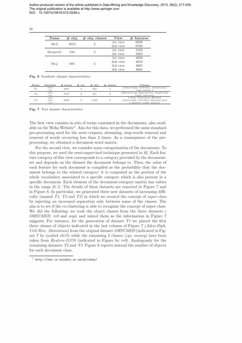
Name # obj. # obj. classes View # features

bbc2 2012 51st view 68382nd view 6790

bbcsport2 544 51st view 31832st view 3203

bbc4 685 5

1st view 46592nd view 46333rd view 46654th view 4684

Fig. 6 Synthetic dataset characteristics.

Name Datasets # terms # cat. # obj. # classes Classes

T1oh15

3987 2 833 5Aden-Diph, Cell-Mov, Aluminium

re0 cpi, money

T2oh15

3197 2 461 5Blood-Coag, Enzyme-Act, Staph-Inf

re0 jobs, reserves

T3wap

8282 3 2129 9 Film, Television, Health

oh15 Aden-Diph, Cell-Mov, Enzyme-Actre0 interest, trade, money

Fig. 7 Text dataset characteristics.

The first view consists in sets of terms contained in the documents, also avail-able on the Weka Website1. Also for this data, we performed the same standardpre-processing used for the news corpora: stemming, stop-words removal andremoval of words occurring less than 3 times. As a consequence of the pre-processing, we obtained a document-word matrix.

For the second view, we consider some categorization of the documents. Tothis purpose, we used the semi-supervised technique presented in [6]. Each fea-ture category of this view corresponds to a category provided by the document-set and depends on the dataset the document belongs to. Then, the value ofeach feature for each document is compiled as the probability that the doc-ument belongs to the related category: it is computed as the portion of thewhole vocabulary associated to a specific category which is also present in aspecific document. Each element of the document-category matrix has valuesin the range [0, 1]. The details of these datasets are reported in Figure 7 andin Figure 8. In particular, we generated three new datasets of increasing diffi-culty (named T1, T2 and T3) in which we created the concept of super-classby injecting an increased separation only between some of the classes. Theaim is to see if the co-clustering is able to recognize the concept of super-class.We did the following: we took the object classes from the three datasets (OHSUMED, re0 and wap) and mixed them as the information in Figure 7suggests. For instance, for the generation of dataset T1 we placed the firstthree classes of objects indicated in the last column of Figure 7 (Aden-Diph,

Cell-Mov, Aluminium) from the original dataset OHSUMED (indicated in Fig-ure 7 by symbol oh15) while the remaining 2 classes (cpi, money) have beentaken from Reuters-21578 (indicated in Figure by re0). Analogously for theremaining datasets T2 and T3. Figure 8 reports instead the number of objectsfor each document class.

1 http://www.cs.waikato.ac.nz/ml/weka/


http://www.cs.waikato.ac.nz/ml/weka/

29

Class Name # obj. Class Name # obj.

Aden-Diph 56 Cpi 60Cell-Mov 106 Money 608Aluminium 53 Interest 219Blood-Coag 69 Trade 319Enzyme-Act 154 Film 196Staph-Inf 157 Television 130

Jobs 39 Health 341Reserves 42

Fig. 8 Classes distributions for text datasets.

Name # words # obj. # classes Classes

I1 114 630 7sunsets, tigers, train,

swimmers, formula One car,skyscrapers, war airplanes

I2 116 541 6bears, deers, horses,cliffs, birds, bridges

I3 170 1171 13sunsets, tigers, train, swimmers,

formula One car, skyscrapers, war airplanes, bridges,bears, deers, horses, cliffs, birds,

Fig. 9 Image dataset characteristics.

The last group of datasets are extracted from the Corel Benchmark2. Thisbenchmark has already been used in [3], and we use a similar pre-processing.It consists of 5000 images from 50 Corel Stock Photo CDs. Each CD contains100 images on the same topic. The original dataset has 4500 training imagesand 500 test images. Here, we consider only the 4500 training images for ourexperiments. Every image has a caption and an annotation. The caption is abrief description of the scene and the annotation is a list of objects (entities, orsegments) that appear in the image. On overall, 371 words and 42379 entitiesare used to describe the collection. We built two different views: the first viewis based on the caption words, the second view is based on blobs. A blob is aportion of the image in which a user has recognized a particular entity. It issimilar to a concept. In order to obtain blobs, we clustered (with a k-means

algorithm) all the entities into 3000 groups (blobs). Each image is mappedonto the set of blobs or entities represented in the image itself. This modelleads to a representation analogous to the bag-of-words model (BOW) oftenused in text processing. For our experiments, we built three different datasets(details are reported in Figure 9). Each of the generated dataset has balancedclasses represented by an average of 90 objects.

5.3 Results and discussion

We now analyze in detail the different aspects of our experimental evaluation.First, we compare the behavior of our algorithm to the three competitors. Sec-ond, we assess the significance of the results statistically. Third, we study thevariability of the number of detected clusters. Then, we perform an in-depthqualitative analysis of the specific results. Finally, we provide a scalabilitystudy.

2 http://kobus.ca/research/data/eccv_2002


http://kobus.ca/research/data/eccv_2002

30

CoStar Comraf SRC NMF

bbc2 0.68 ± 0.02 0.58 ± 0.04 0.31 ± 0.11 0.5 ± 0.04bbcsport2 0.69 ± 0.06 0.09 ± 0.05 0.24 ± 0 0.57 ± 0.01bbc4 0.68 ± 0.03 0.41 ± 0.03 0.33 ± 0.04 0.45 ± 0.0

I1 0.88 ± 0.04 0.85 ± 0.05 0.80 ± 0.11 0.86 ± 0.06I2 0.75 ± 0.04 0.66 ± 0.05 0.61 ± 0.09 0.74 ± 0.04I3 0.76 ± 0.03 0.75 ± 0.04 0.61 ± 0.11 0.73 ± 0.06

T1 0.72 ± 0 0.50 ± 0.03 0.23 ± 0.05 0.49 ± 0.01T2 0.73 ± 0.1 0.35 ± 0.03 0.33 ± 0.08 0.58 ± 0.02T3 0.71 ± 0.02 0.66 ± 0 0.55 ± 0.06 0.63 ± 0.02

Fig. 10 Normalized Mutual Information results.

CoStar Comraf SRC NMF

bbc2 0.67 ± 0.03 0.42 ± 0.05 0.18 ± 0.08 0.48 ± 0.06bbcsport2 0.58 ± 0.14 0.23 ± 0.04 0.14 ± 0.09 0.56 ± 0.02bbc4 0.56 ± 0.2 0.34 ± 0.05 0.16 ± 0.06 0.41 ± 0.0

I1 0.83 ± 0.09 0.80 ± 0.08 0.69 ± 0.11 0.79 ± 0.1I2 0.72 ± 0.07 0.55 ± 0.06 0.51 ± 0.09 0.67 ± 0.07I3 0.50 ± 0.11 0.62 ± 0.06 0.43 ± 0.13 0.61 ± 0.09

T1 0.73 ± 0 0.23 ± 0.05 0.09 ± 0.09 0.23 ± 0.02T2 0.68 ± 0 0.19 ± 0.04 0.18± 0.09 0.48 ± 0.01T3 0.44 ± 0.02 0.42 ± 0.03 0.36 ± 0.08 0.44 ± 0.04

Fig. 11 Adjusted Rand Index results.

5.3.1 CoStar against competitors

In Figure 10 and 11, we report the average and standard deviation of theperformance indexes for each dataset and each clustering approach. We canobserve that CoStar outperforms all other approaches on NMI index andachieves the best results on all the datasets except I3 when considering theARI index. We recall that CoStar does not require any parameter. Despitethis, it finds always high-quality partitions, while the other approaches do nottake advantage of the additional information of the correct number of clusters.

Notice that CoStar always outperforms SRC. On the other hand, Comraf

achieves comparable results over the Images datasets. This is not surprising,since Comraf is suited for this specific application domain. But, when apply-ing Comraf on the text datasets, it returns very poor results regarding bothmeasures. NMF performs better than Comraf on text data, and has similarresults on Corel Benchmarks.

5.3.2 Statistical significance of the results

To assess the statistical quality of our approach we use the Friedman statisticand the Nemenyi test [10]. These techniques are usually employed to evaluatethe statistical relevance of results of different classifiers over multiple datasets.We briefly summarize the Friedman test:


31

1. the performance of each method (in terms of a given evaluation measuresuch as ARI or NMI) is determined on each dataset;

2. the methods are ranked for each dataset according to these results, thebest performing algorithm getting the rank of 1, the second best rank 2,and so on ;

3. for each method, its average rank Rj w.r.t. the datasets is computed;4. finally, the Friedman statistic is computed thanks to the following formula:

Q =12N

k(k + 1)

k∑

j=1

R2j −

k(k + 1)2

4

where N is the number of datasets and k is the number of methods thatare compared.

On the null hypothesis, where is no difference among the k sets of measures,

the average rank should approximate (k+1)2 . When N and k are large (i.e.

N > 15 and k > 4), the probability distribution of Q can be approximated bythat of a chi-square distribution with k − 1 degrees of freedom. In this casethe p-value is given by P (χ2

k−1 ≥ Q). If N or k is small, the approximation tochi-square becomes poor and the p-value should be obtained from tables of Qspecially prepared for the Friedman test.

We compare ARI and NMI results of CoStar and its competitors (SRC,ComRaf and NMF) on the 9 datasets and compute the associated Q values:we obtain 21.63 and 22.73 for ARI and NMI respectively. As the critical valueat significance level α = 0.01 is equal to 10.73 (see [33,31]) and is smaller thanthe Q values, we decide to reject the null hypothesis for both measures.

We can now proceed with the post-hoc Nemenyi test. According to this test,the performance of two algorithms is significantly different if the correspondingaverage ranks differ by at least the critical difference:

CD = qα

√

k(k + 1)

6N

where α is the significance level (α = 0.10 in our case) and qα is the criticalvalue for the two tailed Nemenyi test [10]. We compare the 4 methods at thecritical value q0.10 = 2.291. The ranking table is shown in Figure 12 (top). Thecritical difference between average ranks is CD = 1.394 (for ARI and NMI).Figure 12 (bottom) shows the difference between average ranks for both ARIand NMI. In the first case, CoStar is significantly different from ComRaf

and SRC. In the second case, it performs significantly better than all othercompetitors.

5.3.3 Number of detected clusters

Since CoStar may find different numbers of clusters at each execution, we ranthe algorithm 100 times and evaluate the variability of this result. In Figure 13,


32

Average ranking

Methods ARI NMI

CoStar 1.2 1NMF 2.2 2.4ComRaf 2.6 2.7SRC 4 3.9

ARI NMF ComRaf SRC

CoStar 1 1.4 2.8

NMF - 0.4 1.8

ComRaf - - 1.4

SRC - - 0

NMI NMF ComRaf SRC

CoStar 1.4 1.7 2.9

NMF - 0.3 1.5

ComRaf - - 1.2SRC - - 0

Fig. 12 Average Ranking results for the Nemenyi Test (top); Difference between averageranks for ARI and NMI evaluation measures (bottom).

0

20

40

60

80

100

3 3.5 4 4.5 5 5.5 6

num

ber

of tr

ials

number of clusters

(a)

0

20

40

60

80

100

3 3.5 4 4.5 5 5.5 6 6.5 7

num

ber

of tr

ials

number of clusters

(b)

0

20

40

60

80

100

2 3 4 5 6 7 8 9 10 11

num

ber

of tr

ials

number of clusters

(c)

Fig. 13 Distribution of CoStar number of clusters on (a) bbc2 (b) bbcsport2 (c) bbc4.

0

20

40

60

80

100

1 1.5 2 2.5 3

num

ber

of tr

ials

number of clusters

(a)

0

20

40

60

80

100

2 2.5 3 3.5 4 4.5 5

num

ber

of tr

ials

number of clusters

(b)

0

20

40

60

80

100

2 2.5 3 3.5 4 4.5 5

num

ber

of tr

ials

number of clusters

(c)

Fig. 14 Distribution of the number of clusters of CoStar on (a) T1 (b) T2 (c) T3.

14 and 15, we report the distributions of the number of row clusters for thethree groups of datasets.

On bbc2 and bbcsport2, CoStar produces most of the times partitionswith the correct number of clusters (see Figure 13). However, the resultingpartitions on bbc4 contain 5 or 6 clusters to the same extent.

Now consider the three textual datasets (see Figure 14). By analyzing theresults, we found that CoStar recognizes the “super-classes” correspondingto the originating dataset to which the document belongs to. For instance,for T1 there are two super-classes: one from oh15 and one from re0. This isreasonable because they represent two types of dictionary: a biology-centeredone and a news-centered one. The same phenomenon happens for the other


33

0

20

40

60

80

100

4 5 6 7 8 9

num

ber

of tr

ials

number of clusters

(a)

0

20

40

60

80

100

3 4 5 6 7 8

num

ber

of tr

ials

number of clusters

(b)

0

20

40

60

80

100

6 7 8 9 10 11 12 13

num

ber

of tr

ials

number of clusters

(c)

Fig. 15 Distribution of the number of clusters of CoStar on (a) I1 (b) I2 (c) I3.

two textual datasets. Furthermore, the found number of clusters remains quitestable, in particular for T1 and T2.

Figure 15 shows the distribution of the number of row clusters for theCorel benchmark. First, CoStar detects most of the time the correct numberof clusters (7) when applied to I1. When processing I2, the algorithm findsthree different values of cluster numbers for the row partition: 5, 6 and 7.Notice that in this case, the correct number is 6, which is very close to theaverage of the detected number of clusters. For I3, which is a hard contextfor a clustering algorithm, the distribution of the number of detected clustersmay be approximated with a normal distribution with a mean of 9, while thenumber of built-in classes is 13.

5.3.4 A qualitative evaluation

We now show an example to provide some insights about the kind of resultsour algorithm is able to provide. To this purpose, we choose a specific resultof the I2 image dataset. In particular, among the 100 runs of CoStar, wechoose the one providing the result with the highest value on the objectivefunction computed over the row space (τX|Y).

To provide a readable description of each cluster, we perform a similarprocess to the one used in CoStar when optimizing the objective functions.The goal is to select a subset of elements within each cluster that representsand summarizes the content of the whole cluster. For any given cluster, wetry to remove each of its elements and compute the ∆τ (see Section 4) thatcorresponds to this removal. In this case we use δτ as an evaluation functionof the single cluster elements. We assign to each object the ∆τ (maximumin absolute value) that as a consequence of the movement causes the highestreduction of the objective function value. Finally, we rank all the elements bythe obtained values of ∆τ , and select the top k objects as representatives. No-tice that we use ∆τX|Y

to rank images, and ∆τY k|X

to rank words (see Section

4). We report the cluster descriptions for the textual view of I2 in Figure 16.The reader can observe that the algorithm returns five well-separated clustersof words. The first cluster gathers words around polar animals; the second oneis about bridges, coasts and waterways; the topic of the third one is around


34

animal with horns, the fourth one talks of horses and the last one is aboutbirds and places where they live.

bear, polar, black, snow, antlers, grizzly, elk,ice, tundra, grassbridge, water, coast, arch, hills, sky, waves,beach, boats, steeldeer, white-tailed, mule, horns, slope, fawnhorses, foals, mare, field, fence, bushbirds, nest, branch, fly, tree, leaf, wood, wings,stick, baby

Fig. 16 Word clusters for image dataset 2.

Figure 17 resumes the descriptions of the clusters obtained over the images.Using the top 5 ranked images, we distinguish five clusters: Clusters1 is aboutanimals (reindeer and bears) that live in tundra or polar climate regions;Clusters2 contains pictures of birds; Cluster3 is about horses; Cluster4 isabout coasts and bridges; finally, Cluster5 contains pictures of deer. Noticealso that in this particular case it is possible to map each cluster of imagesonto a cluster of words and vice versa.

CLUSTER 1

CLUSTER 3

CLUSTER 2

CLUSTER 4

CLUSTER 5

Fig. 17 I2 dataset with 5 representative images for each cluster.

5.3.5 Scalability evaluation

We now analyze the time performances of CoStar. We did not perform com-parisons with the competitors since all algorithms are written in different pro-gramming languages, but the reader may refer to Section 4.4 for a theoreticalcomplexity comparison. Here, we focus our analysis on how the number of fea-


35

ture spaces and the number of objects influence the computational time (seeFigure 18).

For the first experiment, we generate several synthetic boolean datasetsvarying the number of feature spaces. Each feature space contains 1000 fea-tures. We let the number of feature spaces vary from 2 to 10. The numberof row objects varies from 500 to 2 000. Data are generated by considering auniform distribution and an average matrix density of 5%. The related timecurves are depicted in Figure 18(a). We observe that CoStar has reasonabletime performances on high-order and high dimensional data. As expected, thebehavior is linear w.r.t. the number of feature spaces.

The last experiment allows us to study the scalability of our algorithmswhen applied to large datasets. In this case, the number of spaces is fixed (2),while we let the number of objects vary from 1 000 to 10 000. Furthermore, werepeated this experiment varying the number of features per space from 500to 2 500. As shown in Figure 18(b), even though the complexity of CoStar

is quadratic in the number of objects/features, in practice, the computationaltime increases linearly with the number of objects.

5.4 Empirical Convergence over Synthetic Data

In this subsection we empirically evaluate the convergence of our method overa synthetic dataset where we know in advance the inner structure. In particularwe consider a Boolean dataset D over O (1 000 objects) and F = F 1, F 2(1000 features for each views). The synthetic dataset has a perfect block nestedstructure with perfect partitions CO1 × CF 1 and CO2 × CF 2 . We have builtCO1 ×CF 1 to have two blocks structure (two perfect clusters over the objectsand two perfect clusters over the features). In the same way CO2 × CF 2 hasa four blocks structure (four perfect clusters over the objects and four perfectclusters over the features).

Let us consider a parameter p that is the probability to flip a Booleanvalue uniformly at random in D and denote by Dp the resulting dataset. Inour experiment we vary p over 5%, 10%, 15% and 20%.

In order to evaluate the quality of the non-dominated solutions, we fol-low the protocol proposed in [20] and [22]. Given a dataset Dp we perform30 runs. Then we define Zall as the union of the obtained solutions. Notethat Zall could contain both dominated and non-dominated vectors, since asolution may dominate another. For this reason we define Z⋆ as the set ofnon-dominated vectors of Zall. Second, we define zmin = (zmin

1 , . . . , zminN+1)

and zmax = (zmax1 , . . . , zmax

N+1), where zmink (resp. zmax

k ) denotes the lower

(resp. upper) bound of the kth objective for all the points contained in Zall.In order to give a roughly equal range to the objective functions, the values

are normalized with respect to zmin and zmax (value−zmin

zmax−zmin ). Note that after

the normalization step zmin is equal to 0N+1 and zmax is equal to 1N+1.Given a solution S, in order to measure the quality of S in comparison

to Z⋆, we compute the difference between these two sets by using the unary


36

0

500

1000

1500

2000

2500

2 4 6 8 10

Run

ning

Tim

e [s

econ

d]

Number of spaces

500 objs1000 objs1500 objs2000 objs

(a)

0

2000

4000

6000

8000

10000

1000 2000 3000 4000 5000 6000 7000 8000 9000 10000

Run

ning

Tim

e [s

econ

d]

Number of objects

500 features1000 features1500 features2000 features2500 features

(b)

Fig. 18 Running time of CoStar varying the number of feature spaces and objects

hypervolume metric [20], where the vector zmin = 0N+1 is the reference point,as it corresponds to the lower bound of the N + 1 normalized objective func-tions. The hypervolume difference indicator (IH) computes the portion of theobjective space that is weakly-dominated by Z⋆ and not by S. The closer this


37

measure to 0, the better the approximation S. Figure 19 illustrates this mea-sure. The light gray area corresponds to the hypervolume difference indicator.

Reference point

Dominated subspace by Z*

Fig. 19 Illustration of the hypervolume difference indicator.

At each iteration we compute the average of hypervolume difference indi-cator IH of the objective functions vectors S of the 30 runs. The maximumnumber of iterations is set to 10000 using the general rules employed in theexperiments (10×max(m,N ) where m and N are the number of objects andfeatures respectively). Using this measure, we evaluate the volume of the domi-nated portion of the objective space and the convergence to a stable solution ofCoStar. This process is repeated for each value of p. The results are reportedin Figure 20.

In Figure 20, we observe that CoStar converges always to very similarsolutions in all the runs with different values of p. As we state in Section4.2, we can notice that at each iteration CoStar converges to a Pareto localoptimum with respect the neighborhood. It is interesting to notice that, inthis case, the algorithm converges to a stable solution very early w.r.t. themaximum number of iterations Niter foreseen in CoStar. We empiricallyobserve the same phenomenon on the real datasets, too. In particular we haveobserved that the maximum number of iterations is always an upper bound ofthe real number of steps needed by CoStar to obtain the final stable solution.

6 Conclusion

Heterogeneous star-structured data are very common in real world applica-tions. In this paper we presented CoStar, a novel algorithm that deals withthis kind of data. Unlike previous approaches, CoStar is totally parameter-less: this means that it does not require either the number of object clustersor the number of feature clusters for each of the feature spaces. Our approachemploys a Pareto-dominance approach to optimize a set of measures for cross-association in contingency tables which we extended to a high-dimensional


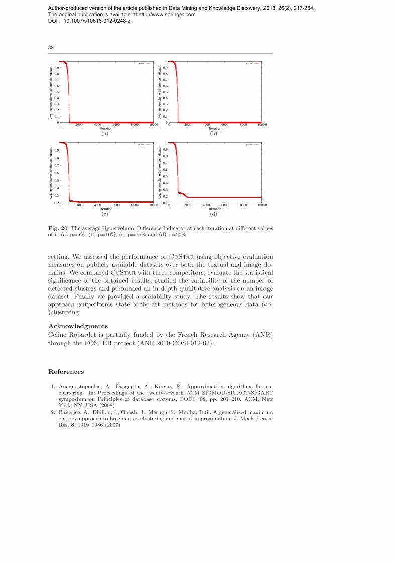
38

0

0.1

0.2

0.3

0.4

0.5

0.6

0.7

0.8

0.9

1

0 2000 4000 6000 8000 10000

Avg

. Hyp

ervo

lum

e D

iffer

ence

Indi

cato

r

Iteration

p=5%

(a)

0

0.1

0.2

0.3

0.4

0.5

0.6

0.7

0.8

0.9

1

0 2000 4000 6000 8000 10000

Avg

. Hyp

ervo

lum

e D

iffer

ence

Indi

cato

r

Iteration

p=10%

(b)

0.2

0.3

0.4

0.5

0.6

0.7

0.8

0.9

1

0 2000 4000 6000 8000 10000

Avg

. Hyp

ervo

lum

e D

iffer

ence

Indi

cato

r

Iteration

p=15%

(c)

0.1

0.2

0.3

0.4

0.5

0.6

0.7

0.8

0.9

1

0 2000 4000 6000 8000 10000

Avg

. Hyp

ervo

lum

e D

iffer

ence

Indi

cato

r

Iteration

p=20%

(d)

Fig. 20 The average Hypervolume Difference Indicator at each iteration at different valuesof p. (a) p=5%, (b) p=10%, (c) p=15% and (d) p=20%

setting. We assessed the performance of CoStar using objective evaluationmeasures on publicly available datasets over both the textual and image do-mains. We compared CoStar with three competitors, evaluate the statisticalsignificance of the obtained results, studied the variability of the number ofdetected clusters and performed an in-depth qualitative analysis on an imagedataset. Finally we provided a scalability study. The results show that ourapproach outperforms state-of-the-art methods for heterogeneous data (co-)clustering.

Acknowledgments

Celine Robardet is partially funded by the French Research Agency (ANR)through the FOSTER project (ANR-2010-COSI-012-02).

References

1. Anagnostopoulos, A., Dasgupta, A., Kumar, R.: Approximation algorithms for co-clustering. In: Proceedings of the twenty-seventh ACM SIGMOD-SIGACT-SIGARTsymposium on Principles of database systems, PODS ’08, pp. 201–210. ACM, NewYork, NY, USA (2008)

2. Banerjee, A., Dhillon, I., Ghosh, J., Merugu, S., Modha, D.S.: A generalized maximumentropy approach to bregman co-clustering and matrix approximation. J. Mach. Learn.Res. 8, 1919–1986 (2007)


39

3. Bekkerman, R., Jeon, J.: Multi-modal clustering for multimedia collections. In: Com-puter Vision and Pattern Recognition, IEEE Computer Society Conference on Visionand Pattern Recognition, pp. 1–8 (2007)

4. Bickel, S., Scheffer, T.: Multi-view clustering. In: ICDM, pp. 19–26 (2004)5. Chakrabarti, D., Papadimitriou, S., Modha, D.S., Faloutsos, C.: Fully automatic cross-

associations. In: KDD, pp. 79–88 (2004)6. Chen, Y., Wang, L., Dong, M.: Semi-supervised document clustering with simultaneous

text representation and categorization. In: ECML/PKDD (1), pp. 211–226 (2009)7. Chen, Y., Wang, L., Dong, M.: Non-negative matrix factorization for semisupervised

heterogeneous data coclustering. IEEE Trans. Knowl. Data Eng. 22(10), 1459–1474(2010)

8. Cho, H., Dhillon, I.S., Guan, Y., Sra, S.: Minimum sum-squared residue co-clusteringof gene expression data. In: Proceedings of SIAM SDM 2004 (2004)

9. Cleuziou, G., Exbrayat, M., Martin, L., Sublemontier, J.H.: Cofkm: A centralizedmethod for multiple-view clustering. In: ICDM, pp. 752–757 (2009)

10. Demsar, J.: Statistical comparisons of classifiers over multiple data sets. Journal ofMachine Learning Research 7, 1–30 (2006)

11. Dhillon, I.S., Mallela, S., Modha, D.S.: Information-theoretic co-clustering. In: Proc.ACM SIGKDD 2003, pp. 89–98. ACM Press, Washington, USA (2003)

12. Forman, G.: An extensive empirical study of feature selection metrics for text classifi-cation. J. Mach. Learn. Res. 3, 1289–1305 (2003)

13. Gao, B., Liu, T.Y., Ma, W.Y.: Star-structured high-order heterogeneous data co-clustering based on consistent information theory. In: ICDM ’06: Proceedings of theSixth International Conference on Data Mining, pp. 880–884 (2006)

14. Goodman, L.A., Kruskal, W.H.: Measures of association for cross classification. Journalof the American Statistical Association 49, 732–764 (1954)

15. Greco, G., Guzzo, A., Pontieri, L.: Co-clustering multiple heterogeneous domains: Linearcombinations and agreements. IEEE Transactions on Knowledge and Data Engineering99 (2009)

16. Hubert, L., Arabie, P.: Comparing partitions. Journal of Classification 2(1), 193–218(1985)

17. Ienco, D., Pensa, R.G., Meo, R.: Parameter-free hierarchical co-clustering by n-ary splits.In: Proceedings of ECML/PKDD 2009, Lecture Notes in Computer Science, vol. 5781,pp. 580–595. Springer (2009)

18. Jaszkiewicz, A.: Genetic local search for multi-objective combinatorial optimization.European Journal Of Operational Research 137(1), 50–71 (2002)

19. Keogh, E., Lonardi, S., Ratanamahatana, C.A.: Towards parameter-free data mining.In: Proceedings of the tenth ACM SIGKDD international conference on Knowledgediscovery and data mining, KDD ’04, pp. 206–215. ACM, New York, NY, USA (2004)

20. Knowles, J., Thiele, L., Zitzler, E.: A Tutorial on the Performance Assessment ofStochastic Multiobjective Optimizers. TIK Report 214, Computer Engineering andNetworks Laboratory (TIK), ETH Zurich (2006)

21. Lee, D.D., Seung, D.D.: Algorithms for non-negative matrix factorization. In: T.K. Leen,T.G. Dietterich, V. Tresp (eds.) Advances in Neural Information Processing Systems,13, pp. 556–562 (2001)

22. Liefooghe, A., Humeau, J., Mesmoudi, S., Jourdan, L., Talbi, E.G.: On dominance-based multiobjective local search: design, implementation and experimental analysis onscheduling and traveling salesman problems. Journal of Heuristics pp. 1–36 (2011)

23. Long, B., Zhang, Z.M., Wu, X., Yu, P.S.: Spectral clustering for multi-type relationaldata. In: ICML ’06: Proceedings of the 23rd international conference on Machine learn-ing, pp. 585–592 (2006)

24. Long, B., Zhang, Z.M., Yu, P.S.: A probabilistic framework for relational clustering. In:KDD ’07: Proceedings of the 13th ACM SIGKDD international conference on Knowl-edge discovery and data mining, pp. 470–479 (2007)

25. Paquete, L.: Stochastic Local Search Algorithms for Multiobjective Combinatorial Op-timization: Methods and Analysis, vol. 295. AKA Verlag/ IOS Press (2006)

26. Paquete, L., Stutzle, T.: A study of stochastic local search algorithms for the biobjectiveqap with correlated flow matrices. European Journal of Operational Research 169(3),943 – 959 (2006)


40

27. Pensa, R.G., Boulicaut, J.F.: Constrained co-clustering of gene expression data. In:Proceedings of SIAM SDM 2008, pp. 25–36 (2008)

28. Ramage, D., Heymann, P., Manning, C.D., Garcia-Molina, H.: Clustering the taggedweb. In: WSDM, pp. 54–63 (2009)

29. Robardet, C., Feschet, F.: Comparison of three objective functions for conceptual clus-tering. In: Proceedings PKDD’01, LNAI, vol. 2168, pp. 399–410. Springer (2001)

30. Robardet, C., Feschet, F.: Efficient local search in conceptual clustering. In: ProceedingsDS’01, LNCS, vol. 2226, pp. 323–335. Springer (2001)

31. Sheskin, D.J.: Handbook of Parametric and Nonparametric Statistical Procedures, 4edn. Chapman & Hall/CRC (2007)

32. Strehl, A., Ghosh, J.: Cluster ensembles — a knowledge reuse framework for combiningmultiple partitions. Journal of Machine Learning Research 3, 583–617 (2002)

33. Zar, J.H.: Biostatistical Analysis (4th Edition). Prentice Hall (1998)


parameter-less co-clustering for star-structured

Documents