parameter space exploration of full system...
TRANSCRIPT
PECOSPredictive Engineering and Computational Sciences
Parameter Space Exploration of Full SystemSimulations
Roy H. Stogner
The University of Texas at Austin
October 6, 2010
Roy H. Stogner Full System Simulation October 6, 2010 1 / 33

Introduction
Full System Simulation• All Relevant Physics
I FlowI TransportI Reacting ChemistryI Surface Reaction, AblationI Radiation, Reradiation
• Forward UncertaintyPropagation
I Calibrated Input ParameterPDFs
I → Output Quantity of InterestStatistics
Coupled Subsystems& Coupled Submodels
Fewer, more difficult experiments
Isolated Components & Sub Models
Many "Simple" Experiments
Increasing Complexity
& Cost
Full SystemRare
Experiments
Prediction of Quantity of Interest
Full System Validation
Coupled Calibration& Validation
Component Calibration& Validation
Roy H. Stogner Full System Simulation October 6, 2010 2 / 33

Challenges
Uncertainty Quantification• High individual forward solve cost
• High parameter count
Verification• Code complexity
• Lacking analytical solutions to complex physics
• Sole interest: Quantity of Interest functionals
Validation• Validation cycle
I Modeling informs research informs modelingI FSS results inform model development, data collection
Roy H. Stogner Full System Simulation October 6, 2010 3 / 33
Multiphysics Coupling
1e-06
1e-05
0.0001
0.001
0.01
0.1
1
0 0.05 0.1 0.15 0.2
Mass F
raction
Distance (m)
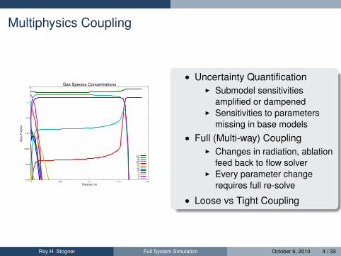
Gas Species Concentrations
C2HN2O2NOCOC2C3CNH2CNOH
• Uncertainty QuantificationI Submodel sensitivities
amplified or dampenedI Sensitivities to parameters
missing in base models• Full (Multi-way) Coupling
I Changes in radiation, ablationfeed back to flow solver
I Every parameter changerequires full re-solve
• Loose vs Tight Coupling
Roy H. Stogner Full System Simulation October 6, 2010 4 / 33

DPLR++
Acknowledgements
DPLR• Michael Wright
• Todd White
• Mike Barnhardt
DPLR++• Paul Bauman
• Rochan Upadhyay
• Andre Maurente
• Karl Schulz
Roy H. Stogner Full System Simulation October 6, 2010 5 / 33

DPLR++
Methodology
Forward UQ Propagation Setup• Off-baseline perturbations resume from hand-converged baseline
• Dakota ILHS study generation, modified preprocessor builds inputworkspaces
• Input samples run on HeraI 80 processors per sampleI 1024 total samplesI 5 hours runtime per sample
• Automatic detection/resumption of failed runs
Postprocessing• Quantities of interest from DPLR, coupling enhancements, postflow
• “make summarize” - extraction, collection, calculations
• Makefile-based job submission, lonestar/hera options
Roy H. Stogner Full System Simulation October 6, 2010 6 / 33

Forward UQ
Uncertain Parameters
Submodel Uncertainties• Hypersonic Flow
I Trajectory peak heating point• Velocity• Freestream conditions
I Chemical reaction ratesI Diffusive fluxesI Turbulent mixing
• RadiationI AbsorptivityI Model Error
• AblationI Virgin, char densitiesI Reaction rates, equilibria
∼ 300 independent parametersRoy H. Stogner Full System Simulation October 6, 2010 7 / 33

Forward UQ
Monte Carlo Integration
Errors
• qMC − q variance: σ2e[q] = σ2
Ns
•(σMCq
)2 − σ2q variance: σ2
e[σ2] = σ4(
2Ns−1 + κ
Ns
)• PMC
C − PC variance: σ2e[PC ] =
PC−P 2C
Ns
• Sampling-based scheme errors are PDFs
• Errors based on variance σ2 of sampled entity
• Error “bound” width: σe ∝ N−1/2
Roy H. Stogner Full System Simulation October 6, 2010 8 / 33

Forward UQ
Latin Hypercube Sampling
Algorithm• Form quantile bins in each
parameter• Permute samples to bins
I Reducing correlations
• Randomly place eachsample within its bin
Uses• Reduce variance from
additive responsecomponents
• O(N−3/2
)convergence for
separable functions
Roy H. Stogner Full System Simulation October 6, 2010 9 / 33

Forward UQ
Results: Outputs
1.4 1.6 1.8 2 2.2 2.4 2.6 2.8
x 10−5
0
50
100
150
200
250
300
Ablation Rate
Ou
tpu
t S
am
ple
s
4.2 4.4 4.6 4.8 5 5.2 5.4 5.6 5.8 6
x 105
0
50
100
150
200
250
300
Convective Heat Flux
Ou
tpu
t S
am
ple
s
Accuracy• ≈ 2 significant figures on mean
• ≈ 1 significant figure on standard deviation
• ≈ .5 million CPU-hours on Hera
• 50+ million CPU-hours: too much
Roy H. Stogner Full System Simulation October 6, 2010 10 / 33
Forward UQ
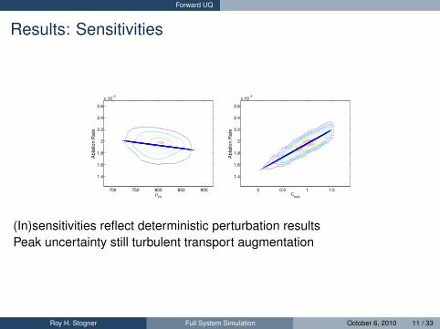
Results: Sensitivities
ρch
Ab
latio
n R
ate
700 750 800 850 900
1.4
1.6
1.8
2
2.2
2.4
2.6
x 10−5
Cturb
Ab
latio
n R
ate
0 0.5 1 1.5
1.4
1.6
1.8
2
2.2
2.4
2.6
x 10−5
(In)sensitivities reflect deterministic perturbation resultsPeak uncertainty still turbulent transport augmentation
Roy H. Stogner Full System Simulation October 6, 2010 11 / 33
Forward UQ
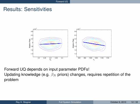
Results: Sensitivities
βN
Ab
latio
n R
ate
0.2 0.25 0.3 0.35 0.4
1.4
1.6
1.8
2
2.2
2.4
2.6
x 10−5
ρv
Ab
latio
n R
ate
900 950 1000 1050 1100 1150
1.4
1.6
1.8
2
2.2
2.4
2.6
x 10−5
Forward UQ depends on input parameter PDFs!Updating knowledge (e.g. βN priors) changes, requires repetition of theproblem
Roy H. Stogner Full System Simulation October 6, 2010 12 / 33

Adjoint-Enabled Forward UQ
Control VariateKnown Surrogate• Quantity of interest q has correlated surrogate statistic qs• “Known” mean qs ≡ E [qs]
cqqs ≡E [(q − q)(qs − qs)]
σqσqs
Variance-reduced statistic
E [q] = E [q − αqs] + E [αqs] = E [s]
s ≡ q − αqs + αqs
σ2s = σ2
q − 2αcqqsσqσqs + α2σ2qs
Integrating s via MC sampling, α ≡ 1, qs → q gives σe[q] → 0.
Roy H. Stogner Full System Simulation October 6, 2010 13 / 33

Adjoint-Enabled Forward UQ
Sensitivity CalculationAdjoint Problem
Ru(u, z; ξ)(u) = Qu(u; ξ)(u) ∀u ∈ U
• Nq adjoint linear solves
• Independent of Nξ
• Much cheaper than highly nonlinear forward problem!
Sensitivity Evaluation
q′ = Qξ(u; ξ)−Rξ(u, z; ξ)
• NqNξ dot products
• libMesh: Finite differenced estimation of Qξ and Rξ
Roy H. Stogner Full System Simulation October 6, 2010 14 / 33
Adjoint-Enabled Forward UQ
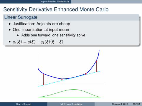
Sensitivity Derivative Enhanced Monte CarloLinear Surrogate• Justification: Adjoints are cheap• One linearization at input mean
I Adds one forward, one sensitivity solve
• qs(ξ) ≡ q(ξ) + qξ(ξ)(ξ − ξ)
Roy H. Stogner Full System Simulation October 6, 2010 15 / 33

Adjoint-Enabled Forward UQ Local Sensitivity Derivatives
Local Sensitivity Derivatives• Wait a minute: ”Adjoints are cheap”
I Forward solve: may be highly nonlinearI Adjoint solve: linear (around forward solution)
• What if we can afford a sensitivity derivative at every sample?
Roy H. Stogner Full System Simulation October 6, 2010 16 / 33

Adjoint-Enabled Forward UQ Local Sensitivity Derivatives
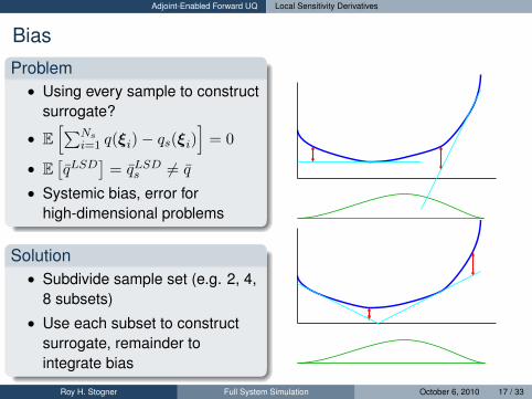
Bias
Problem• Using every sample to construct
surrogate?
• E[∑Ns
i=1 q(ξi)− qs(ξi)]
= 0
• E[qLSD
]= qLSDs 6= q
• Systemic bias, error forhigh-dimensional problems
Solution• Subdivide sample set (e.g. 2, 4,
8 subsets)
• Use each subset to constructsurrogate, remainder tointegrate bias
Roy H. Stogner Full System Simulation October 6, 2010 17 / 33
Adjoint-Enabled Forward UQ Local Sensitivity Derivatives
Bias
Problem• Using every sample to construct
surrogate?
• E[∑Ns
i=1 q(ξi)− qs(ξi)]
= 0
• E[qLSD
]= qLSDs 6= q
• Systemic bias, error forhigh-dimensional problems
Solution• Subdivide sample set (e.g. 2, 4,
8 subsets)
• Use each subset to constructsurrogate, remainder tointegrate bias
Roy H. Stogner Full System Simulation October 6, 2010 17 / 33

Adjoint-Enabled Forward UQ Local Sensitivity Derivatives
Multi Parameter Benchmark Problems
0.01
0.1
1
10 100 1000
Err
or
in A
ppro
xim
ate
d O
utp
ut
Number of Forward Evaluations
Forward UQ Convergence: Exp Benchmark, Mean
MC+SRSSDEMC+SRS
LSDEMC2+SRSLSDEMC4+SRSLSDEMC8+SRS
MC+LHSSDEMC+LHS
LSDEMC2+LHSLSDEMC4+LHSLSDEMC8+LHS
0.01
0.1
1
10 100 1000
Err
or
in A
ppro
xim
ate
d O
utp
ut
Number of Forward Evaluations
Forward UQ Convergence: Exp Benchmark, Mean
MC+SRSSDEMC+SRS
LSDEMC2+SRSLSDEMC4+SRSLSDEMC8+SRS
MC+LHSSDEMC+LHS
LSDEMC2+LHSLSDEMC4+LHSLSDEMC8+LHS
Initial Results• Improved convergence constant
• Higher asymptotic convergence!
Roy H. Stogner Full System Simulation October 6, 2010 18 / 33

Adjoint-Enabled Forward UQ Local Sensitivity Derivatives
Goal-Oriented Refinement
Adaptive Discretization• Estimate error on each cell
I Patch recovery on forward solution• Estimate each cell error contribution to
QoII Patch recovery on adjoint solution
• Refine highest contribution cells first
3 4 5 6 7−3.5
−3
−2.5
−2
−1.5
−1
Log10
(Dofs), Degrees of Freedom
Log 1
0(R
ela
tive E
rror)
Uniform
Flux Jump
Adjoint Residual
Roy H. Stogner Full System Simulation October 6, 2010 19 / 33

Adjoint-Enabled Forward UQ Local Sensitivity Derivatives
Goal-Oriented Error
Quantity of Interest Error
eQ ≡ q − qh ≡ Q(u; ξ)−Q(uh; ξ)
Frechet differentiability of Q gives the highest order error terms
Q(u; ξ)−Q(uh; ξ) = Qu(u; ξ)(u− uh) +RQ
Q(u; ξ)−Q(uh; ξ) = Ru(u, z; ξ)(u− uh)
Frechet differentiability of R gives a useful estimate:
eQ = R(u, z; ξ)−R(uh, z; ξ) +RQ −RR= −R(uh, z; ξ) +RQ −RR
Roy H. Stogner Full System Simulation October 6, 2010 20 / 33

Adjoint-Enabled Forward UQ Local Sensitivity Derivatives
Adjoint Refinement Error Estimator
Error Estimators• R(uh, zh; ξ) is zero, not a good approximation of R(uh, z; ξ)
• Higher order approximation of z is necessary:I Project uh to a refined space.I Jacobian calculation, adjoint solve on refined mesh.I Residual evaluation on refined mesh.
• AdjointRefinementErrorEstimator - not yet implementedI Straightforward extension of UniformRefinementErrorEstimator
RQ and RR at worst are higher order, at best are quadratic in∣∣∣∣u− uh∣∣∣∣.
Error in z will be of the same order as the QoI error, with smallermagnitude.
• Asymptotically bounded effectivity
• Improved QoI estimates
Roy H. Stogner Full System Simulation October 6, 2010 21 / 33

Adjoint-Enabled Forward UQ Local Sensitivity Derivatives
Adjoint Residual Error IndicatorError Indicators• Efficiently bounding eQ via per-element terms
• With our error estimator,
R(uh, z; ξ) =∑E
RE( uh∣∣∣E, z|E ; ξ)
• zh is cheaper than higher order approximation of z
Ignoring higher order terms:
q − qh = −Ru(u, z − zh; ξ)(u− uh)∣∣∣q − qh∣∣∣ ≤ ||Ru||B(U ,V ∗)
∣∣∣∣∣∣u− uh∣∣∣∣∣∣U
∣∣∣∣∣∣z − zh∣∣∣∣∣∣V∣∣∣q − qh∣∣∣ ≤∑
E
∣∣∣∣REu ∣∣∣∣B(UE ,V E∗)
∣∣∣∣∣∣ u|E − uh∣∣∣E
∣∣∣∣∣∣UE
∣∣∣∣∣∣ z|E − zh∣∣∣E
∣∣∣∣∣∣V E
Roy H. Stogner Full System Simulation October 6, 2010 22 / 33

Adjoint-Enabled Forward UQ Local Sensitivity Derivatives
Adjoint Residual Error Indicator
AdjointResidualErrorEstimator Procedure
• Calculate equal-order adjoint solution zh
• Use existing (patch recovery) estimators for∣∣∣∣u− uh∣∣∣∣ and∣∣∣∣z − zh∣∣∣∣ on each element
• Combine element-by-element
AdjointResidualErrorEstimator Limitations• Asymptotic overestimate• No estimation of
∣∣∣∣REu ∣∣∣∣I Would require local DenseMatrix inversion, multiplication, 2-norm
estimate
Roy H. Stogner Full System Simulation October 6, 2010 23 / 33

FIN-S
Acknowledgements
libMesh• Benjamin Kirk
• John Peterson
• Vikram Garg
• Varis Carey
FIN-S• Benjamin Kirk
• Todd Oliver
• Karl Schulz
• Rochan Upadhyay
• Nicholas Malaya
• Kemelli Estacio-Hiroms
Roy H. Stogner Full System Simulation October 6, 2010 24 / 33
FIN-S
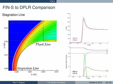
FIN-S to DPLR Comparison
Stagnation Line
x (m)
T(K
)
-0.025 -0.02 -0.015 -0.01 -0.005 00
2000
4000
6000
8000
10000
12000
14000
FIN-SDPLR
x (m)
Spe
cies
Mas
sF
ract
ion
-0.025 -0.02 -0.015 -0.01 -0.005 010-3
10-2
10-1
100
FIN-SDPLR
O2
NO
NO
N2
Roy H. Stogner Full System Simulation October 6, 2010 25 / 33

FIN-S
FIN-S to DPLR Comparison
Flank Line
T (K)
y(m
)
3000 3500 4000 4500 5000 5500 6000 65000.1
0.12
0.14
0.16
0.18
FIN-SDPLR
Species Mass Fraction
y(m
)
10-6 10-5 10-4 10-3 10-2 10-1 1000.1
0.12
0.14
0.16
0.18
FIN-SDPLR
O2
NO
NO
N2
Roy H. Stogner Full System Simulation October 6, 2010 26 / 33
FIN-S
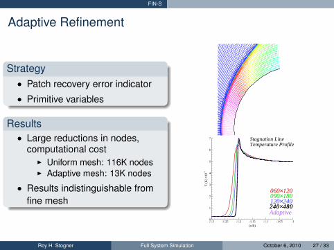
Adaptive Refinement
Strategy• Patch recovery error indicator
• Primitive variables
Results• Large reductions in nodes,
computational costI Uniform mesh: 116K nodesI Adaptive mesh: 13K nodes
• Results indistinguishable fromfine mesh
(x/R)
T(K
)×1
0-3
-1.3 -1.25 -1.2 -1.15 -1.1 -1.05 -10
1
2
3
4
5
6
7
240×480
060×120090×180
Adaptive
120×240
Stagnation LineTemperature Profile
Roy H. Stogner Full System Simulation October 6, 2010 27 / 33
FIN-S
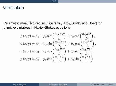
Verification
Parametric manufactured solution family (Roy, Smith, and Ober) forprimitive variables in Navier-Stokes equations:
ρ (x, y) = ρ0 + ρx sin(aρxπx
L
)+ ρy cos
(aρyπyL
),
u (x, y) = u0 + ux sin(auxπx
L
)+ uy cos
(auyπyL
),
v (x, y) = v0 + vx cos(avxπx
L
)+ vy sin
(avyπyL
),
p (x, y) = p0 + px cos(apxπx
L
)+ py sin
(apyπyL
)
Roy H. Stogner Full System Simulation October 6, 2010 28 / 33

FIN-S
VerificationMethod of Manufactured Solutions• Evaluate forcing terms analytically
• Add weighted MASA source functions to residual
• No changes to Jacobian, solver!
∂ρ
∂t+∂(ρu)
∂x+∂(ρv)
∂y= Qρ
∂(ρu)
∂t+∂(ρu2 + p− τxx)
∂x+∂(ρuv − τxy)
∂y= Qu
∂(ρv)
∂t+∂(ρvu− τyx)
∂x+∂(ρv2 + p− τyy)
∂y= Qv
∂(ρe)
∂t+∂(ρuet + pu− uτxx − vτxy + qx)
∂x+∂(ρvet + pv − uτyx − vτyy + qy)
∂y
= Qe
Roy H. Stogner Full System Simulation October 6, 2010 29 / 33

FIN-S
2D N-S MMS Energy TermQe =− apxπpx
L
γ
γ − 1sin(apxπx
L
) [ux sin
(auxπxL
)+ uy cos
(auyπyL
)+ u0
]+apyπpyL
γ
γ − 1cos(apyπy
L
) [vx cos
(avxπxL
)+ vy sin
(avyπyL
)+ v0
]+aρxπρx
2Lcos(aρxπx
L
) [ux sin
(auxπxL
)+ uy cos
(auyπyL
)+ u0
] [[ux sin
(auxπxL
)+ uy cos
(auyπyL
)+ u0
]2+[vx cos
(avxπxL
)+ vy sin
(avyπyL
)+ v0
]2]
− aρyπρy2L
sin(aρyπy
L
) [vx cos
(avxπxL
)+ vy sin
(avyπyL
)+ v0
] [[ux sin
(auxπxL
)+ uy cos
(auyπyL
)+ u0
]2+[vx cos
(avxπxL
)+ vy sin
(avyπyL
)+ v0
]2]
+auxπux
2Lcos(auxπx
L
){[px cos
(apxπxL
)+ py sin
(apyπyL
)+ p0
] 2γ
γ − 1+
+
[3[ux sin
(auxπxL
)+ uy cos
(auyπyL
)+ u0
]2+[vx cos
(avxπxL
)+ vy sin
(avyπyL
)+ v0
]2] [ρx sin
(aρxπxL
)+ ρy cos
(aρyπyL
)+ ρ0
]}− auyπuy
Lsin(auyπy
L
) [ρx sin
(aρxπxL
)+ ρy cos
(aρyπyL
)+ ρ0
] [ux sin
(auxπxL
)+ uy cos
(auyπyL
)+ u0
] [vx cos
(avxπxL
)+ vy sin
(avyπyL
)+ v0
]− avxπvx
Lsin(avxπx
L
) [ρx sin
(aρxπxL
)+ ρy cos
(aρyπyL
)+ ρ0
] [ux sin
(auxπxL
)+ uy cos
(auyπyL
)+ u0
] [vx cos
(avxπxL
)+ vy sin
(avyπyL
)+ v0
]+avyπvy
2Lcos(avyπy
L
){[px cos
(apxπxL
)+ py sin
(apyπyL
)+ p0
] 2γ
γ − 1
+
[[ux sin
(auxπxL
)+ uy cos
(auyπyL
)+ u0
]2+ 3
[vx cos
(avxπxL
)+ vy sin
(avyπyL
)+ v0
]2] [ρx sin
(aρxπxL
)+ ρy cos
(aρyπyL
)+ ρ0
]}
+a2pxπ
2k px cos(apxπx
L
)[ρx sin
(aρxπxL
)+ ρy cos
(aρyπyL
)+ ρ0
]L2R
+a2pyπ
2k py sin(apyπy
L
)[ρx sin
(aρxπxL
)+ ρy cos
(aρyπyL
)+ ρ0
]L2R
−2a2
ρxπ2k ρ2
x
L2Rcos2
(aρxπxL
) [px cos(apxπx
L
)+ py sin
(apyπyL
)+ p0
][ρx sin
(aρxπxL
)+ ρy cos
(aρyπyL
)+ ρ0
]3 −a2ρxπ
2kρx
L2Rsin(aρxπx
L
) [px cos(apxπx
L
)+ py sin
(apyπyL
)+ p0
][ρx sin
(aρxπxL
)+ ρy cos
(aρyπyL
)+ ρ0
]2
−2a2
ρyπ2k ρ2
y
L2Rsin2
(aρyπyL
) [px cos(apxπx
L
)+ py sin
(apyπyL
)+ p0
][ρx sin
(aρxπxL
)+ ρy cos
(aρyπyL
)+ ρ0
]3 −a2ρyπ
2kρy
L2Rcos(aρyπy
L
) [px cos(apxπx
L
)+ py sin
(apyπyL
)+ p0
][ρx sin
(aρxπxL
)+ ρy cos
(aρyπyL
)+ ρ0
]2
+4a2
uxπ2µux
3L2sin(auxπx
L
) [ux sin
(auxπxL
)+ uy cos
(auyπyL
)+ u0
]− 4a2
uxπ2µu2
x
3L2cos2
(auxπxL
)+a2uyπ
2µuy
L2cos(auyπy
L
) [ux sin
(auxπxL
)+ uy cos
(auyπyL
)+ u0
]−
a2uyπ
2µu2y
L2sin2
(auyπyL
)+a2vxπ
2µvxL2
cos(avxπx
L
) [vx cos
(avxπxL
)+ vy sin
(avyπyL
)+ v0
]− a2
vxπ2µv2
x
L2sin2
(avxπxL
)+
4a2vyπ
2µvy
3L2sin(avyπy
L
) [vx cos
(avxπxL
)+ vy sin
(avyπyL
)+ v0
]−
4a2vyπ
2µv2y
3L2cos2
(avyπyL
)− 2apxaρxπ
2k pxρxL2R
cos(aρxπx
L
)sin(apxπx
L
)[ρx sin
(aρxπxL
)+ ρy cos
(aρyπyL
)+ ρ0
]2 −2apyaρyπ
2k pyρyL2R
cos(apyπy
L
)sin(aρyπy
L
)[ρx sin
(aρxπxL
)+ ρy cos
(aρyπyL
)+ ρ0
]2
+4auxavyπ
2µuxvy3L2
cos(auxπx
L
)cos(avyπy
L
)− 2auyavxπ
2µuyvxL2
sin(auyπy
L
)sin(avxπx
L
)
Roy H. Stogner Full System Simulation October 6, 2010 30 / 33

FIN-S
FIN-S+MASA Status
MMS Tested• 2D/3D Euler, perfect gas
• 2D/3D Navier-Stokes, constant viscosity/Pr
Quadratic convergence on smooth problems!
MMS Developed• 2D/3D Navier-Stokes, T /Tv thermal nonequilibrium
MMS in Development• 2D/3D Navier-Stokes, dissociation reactions
• 2D/3D Navier-Stokes, Sutherland viscosity
Multiphysics MMS testing must be modular!
Roy H. Stogner Full System Simulation October 6, 2010 31 / 33

FIN-S
Multiphysics Coupling: Ablation
ChaleurLoosely coupled, Non-overlapping Schwarz iteration
libablationTightly coupled, nonlinear Robin boundary condition
Roy H. Stogner Full System Simulation October 6, 2010 32 / 33

FIN-S
Thank you!
Questions?
Roy H. Stogner Full System Simulation October 6, 2010 33 / 33