Atmos. Chem. Phys., 15, 6775–6788, 2015

www.atmos-chem-phys.net/15/6775/2015/

doi:10.5194/acp-15-6775-2015

© Author(s) 2015. CC Attribution 3.0 License.

Parameterization of convective transport in the boundary layer

and its impact on the representation of the diurnal cycle

of wind and dust emissions

F. Hourdin1, M. Gueye2, B. Diallo1, J.-L. Dufresne1, J. Escribano1, L. Menut1, B. Marticoréna3, G. Siour3, and

F. Guichard4

1Laboratoire de Météorologie Dynamique, CNRS/IPSL/UMPC, Paris, France2LPAOSF, UCAD, Dakar, Sénégal3LISA, UMR CNRS 7583, UPEC, UPD, IPSL, Créteil, France4CNRM-GAME, UMR CNRS 3589, Météo France, Toulouse, France

Correspondence to: F. Hourdin (hourdin@lmd.jussieu.fr)

Received: 16 August 2014 – Published in Atmos. Chem. Phys. Discuss.: 31 October 2014

Revised: 18 February 2015 – Accepted: 07 April 2015 – Published: 18 June 2015

Abstract. We investigate how the representation of the

boundary layer in a climate model impacts the representa-

tion of the near-surface wind and dust emission, with a focus

on the Sahel/Sahara region. We show that the combination of

vertical turbulent diffusion with a representation of the ther-

mal cells of the convective boundary layer by a mass flux

scheme leads to realistic representation of the diurnal cycle

of wind in spring, with a maximum near-surface wind in the

morning. This maximum occurs when the thermal plumes

reach the low-level jet that forms during the night at a few

hundred meters above surface. The horizontal momentum in

the jet is transported downward to the surface by compen-

sating subsidence around thermal plumes in typically less

than 1 h. This leads to a rapid increase of wind speed at

surface and therefore of dust emissions owing to the strong

nonlinearity of emission laws. The numerical experiments

are performed with a zoomed and nudged configuration of

the LMDZ general circulation model coupled to the emis-

sion module of the CHIMERE chemistry transport model, in

which winds are relaxed toward that of the ERA-Interim re-

analyses. The new set of parameterizations leads to a strong

improvement of the representation of the diurnal cycle of

wind when compared to a previous version of LMDZ as well

as to the reanalyses used for nudging themselves. It also gen-

erates dust emissions in better agreement with current esti-

mates, but the aerosol optical thickness is still significantly

underestimated.

1 Introduction

Desert dust is a secondary but significant contributor to atmo-

spheric radiative transfer, with regional signatures dominated

by desert areas like North Africa, which is estimated to con-

tribute 25–50 % of the global dust emissions (Engelstaedter

et al., 2006). This change in radiation may affect the large-

scale circulation by inducing regional contrasts of several

tens of Wm−2 (Yoshioka et al., 2007; Solmon et al., 2008;

Spyrou et al., 2013), as well as the convective processes in

the atmosphere through modulation of the atmospheric static

stability. Dust is more and more often taken into account in-

teractively in global climate simulations, such as those co-

ordinated at an international level in the Coupled Model In-

tercomparison Project (CMIP, Taylor et al., 2012) on which

future climate change estimates are based. Dust is a tracer

of atmospheric motions that sediments into the atmosphere

and can be deposited to the surface rapidly and washed out

by rainfall. One of the important and uncertain dust-related

processes is emission, which depends nonlinearly on the fric-

tion velocity U∗ (Gillette, 1977; Nickling and Gillies, 1989,

1993; Gomes et al., 2003; Rajot et al., 2003; Sow et al., 2009;

Shao et al., 2011).

The emission thus depends on the tail of the near-surface

wind distribution than on the wind mean value. During win-

ter and spring, dust emissions largely occurs in the morning

(see e.g., Schepanski et al., 2009), which coincides with the

daily maximum wind speed in the observations in the Sa-

Published by Copernicus Publications on behalf of the European Geosciences Union.

6776 F. Hourdin et al.: Convective transport in the boundary layer and dust emissions

hel (Parker et al., 2005; Lothon et al., 2008; Guichard et al.,

2009; Schepanski et al., 2009). This maximum is associated

with the low-level jet which forms at a few hundred me-

ters above the surface after sunset, when the near-surface

boundary layer turbulence collapses (see e.g., Bain et al.,

2010; Gounou et al., 2012; Fiedler et al., 2013). After sun-

rise, a convective boundary layer rapidly develops, which

brings momentum from this low-level jet down to the sur-

face and further mixes horizontal momentum over the depth

of the convective boundary layer, typically 2 to 6 km thick

over Sahara and Sahel (see e.g., Cuesta et al., 2009). Todd

et al. (2008) report problems in the representation of the diur-

nal cycle of near-surface wind in a series of simulations with

regional models over the Bodélé region during the Bodex

2005 experiment. They also conclude that the problem comes

more from missing physics in the model than from the grid

resolution. This diurnal cycle is neither well captured in the

ERA-Interim (ERAI) reanalyses (Fiedler et al., 2013) nor in

other state-of-the-art reanalysis data sets as recently shown

by Largeron et al. (2015). Fiedler et al. (2013) report typical

underestimation of 24–50 % for the jet maximum velocity

in the Bodélé region. Todd et al. (2008) and Knippertz and

Todd (2012) underline the importance of a good representa-

tion of the contrast between nocturnal turbulence in a stable

atmosphere and convective transport during the day for the

representation of this nocturnal jet and its impact on surface

wind.

Various approaches have been proposed in the past

decades to represent boundary layer convection. Deardorff

(1970) first noticed that parameterizations of boundary layer

turbulence that are based on eddy or K diffusion fail to rep-

resent the basics of boundary layer convection, which essen-

tially transports heat upward from the surface. This corre-

sponds to upgradient transport of potential temperature since

the atmosphere is generally neutral or even slightly stable

in the so-called “mixed layer” (typically several kilometers

thick in this region of the globe in the afternoon), above the

unstable surface layer (typically a few hundred meters thick).

The counter-gradient term he proposed to reconcile the diffu-

sive formulations with convection conditions was later given

a more explicit formulation based on the non-local aspect of

convective transport by Troen and Mahrt (1986) and by Holt-

slag and Boville (1993). Stull (1984) underlined the impor-

tance of non-local aspects and proposed the “transilience ma-

trices” framework. Chatfield and Brost (1987) first proposed

combining a diffusive approach with a “mass flux” scheme

dedicated to the representation of the boundary layer con-

vection. In this approach, the convection is represented by

splitting the atmospheric column in two compartments: one

associated with the concentrated buoyant updrafts (or ther-

mal plumes) that rise from the surface and the other one

with compensating subsidence around those plumes. This ap-

proach was developed independently by two teams and since

adopted in several groups (Hourdin et al., 2002; Soares et al.,

2004; Siebesma et al., 2007; Pergaud et al., 2009; Angevine

et al., 2010; Neggers et al., 2009; Neggers, 2009; Hourdin

et al., 2013b). It has been shown in particular to open the way

to quite accurate representation of cumulus clouds that form

at the top of convective thermal plumes (Rio and Hourdin,

2008; Jam et al., 2013). The first application of these ideas to

the simulation of the dry convective boundary layer (Hour-

din et al., 2002) demonstrated the capability of the so-called

“thermal plume model” to correctly represent the up-gradient

transport of heat in a slightly stable convective mixed layer.

This approach was shown to also capture well the typical di-

urnal cycle over land, contrasting a thin nocturnal boundary

layer dominated by wind shear-driven turbulent diffusion,

and daily conditions in which the role of the parameterized

turbulent diffusion is confined to the unstable surface layer

while the mass flux scheme accounts for most of the turbu-

lent transport in the mixed layer. This thermal plume model

was developed for the LMDZ atmospheric general circula-

tion model, in which it was activated in particular to perform

a subset of climate simulations for the last CMIP5 exercise

(Hourdin et al., 2013b).

The present study aims at exploring the impact of the

above described parameterizations on the representation of

dust emission and transport and at anticipating future ver-

sions of the climate simulations with interactive aerosols.

For this, the emission module from the chemistry transport

model CHIMERE (Menut et al., 2013) was coupled to the

climate model. We show here how the activation of the ther-

mal plume model leads to a better representation of the diur-

nal cycle of near-surface winds – even better than in current

meteorological reanalyses – and how this better representa-

tion reinforces surface emissions drastically. We focus here

on emissions during the dry season while a companion pa-

per will be devoted to the representation of dust emission by

gusts associated with convection-generated cold pools, for

which a specific parameterization has also been introduced

in LMDZ (Grandpeix and Lafore, 2010; Rio et al., 2009).

In Sect. 2 we present the numerical model and observa-

tions. We then illustrate the impact of the parameterization

of the boundary layer on the near-surface wind distribution

and dust emission using online dust simulations with two ver-

sions of the LMDZ physical package (Sect. 3) and compare

the results with site observations (Sect. 4), before analyzing

in more detail the representation of the mean diurnal cycle

of near-surface wind over the Sahel when the thermal plume

model is activated (Sect. 5) and drawing some conclusions.

2 Methods

2.1 LMDZ5 and IPSL-CM5

The LMDZ dynamical core is based on a mixed finite differ-

ence/finite volume discretization of the primitive equations

of meteorology (approximate form of the conservation laws

for air mass, momentum and potential temperature, under hy-

Atmos. Chem. Phys., 15, 6775–6788, 2015 www.atmos-chem-phys.net/15/6775/2015/

F. Hourdin et al.: Convective transport in the boundary layer and dust emissions 6777

drostatic and “thin layer” approximation) and conservation

equations for trace species. It is coupled to a set of physical

parameterizations. Two versions of the model, LMDZ5A and

LMDZ5B, are considered here that differ by the activation

of a different set of parameterizations for turbulence, con-

vection and clouds. In the “Standard Physics” package (SP)

used in version LMDZ5A (Hourdin et al., 2013a), bound-

ary layer turbulence is parameterized as a diffusion with an

eddy diffusivity that depends on the local Richardson num-

ber. A counter-gradient term on potential temperature (Dear-

dorff, 1972) as well as a dry convective adjustment are added

to handle dry convection cases which often prevail in the

boundary layer. In the “New Physics” package (NP) of ver-

sion LMDZ5B (Hourdin et al., 2013b), the vertical transport

in the boundary layer relies on the combination of a clas-

sical parameterization of turbulent diffusion with the ther-

mal plume model described below (Hourdin et al., 2002; Rio

and Hourdin, 2008). The SP and NP versions also differ by

the representation of deep convection closure and triggering.

However, we will concentrate the present study on the dry

season over West Africa when deep convection does not ac-

tivate. The two versions correspond to the IPSL-CM5A and

CM5B versions of the IPSL coupled model used for CMIP5

(Dufresne et al., 2013).

2.2 The “thermal plume model”

In the NP version, eddy diffusivity Kz is computed based

on a prognostic equation for the turbulent kinetic energy that

follows Yamada (1983). It is mainly active in practice in the

surface boundary layer, typically in the first few hundred me-

ters above surface. It is combined with a mass flux scheme

that represents an ensemble of coherent ascending thermal

plumes as a mean plume. A model column is separated in

two parts: the thermal plume and its environment. The ver-

tical mass flux in the plume fth = ραthwth – where ρ is the

air density, wth the vertical velocity in the plume and αth its

fractional coverage – varies vertically as a function of lat-

eral entrainment eth (from environment to the plume) and

detrainment dth (from the plume to the environment). For

a scalar quantity q (total water, potential temperatures, chem-

ical species, aerosols), the vertical transport by the thermal

plume reads

∂fthqth

∂z= ethq − dthqth, (1)

where qth is the concentration of q inside the plume. Note

that this formulation assumes stationarity of the plume prop-

erties when compared to the timescale of the change in the

explicit model state variables q, a classical approximation in

mass flux parameterizations of convective motions. Here air

is assumed to enter the plume with the mean grid cell concen-

tration q, which is equivalent to neglecting the plume frac-

tion αth in this part of the computation. This approximation

is generally considered as obvious for cumulus convection,

which often covers a very small fraction of the horizontal

surface (e.g., Tiedtke, 1989). It is more questionable for the

boundary layer convection where the fraction is often close

to 5–10 % but the approximation is generally maintained for

numerical reasons1. The approximation is, however, proba-

bly less an issue than the specification of e and d and does

not prevent accurate comparison with large eddy simulations

(Hourdin et al., 2002).

The particular case of q ≡ qth ≡ 1 gives the continuity

equation that relates eth, dth and fth. The vertical velocitywth

in the plume is driven by the plume buoyancy g(θth− θ)/θ ,

where θ is the mean potential temperature in the grid box and

θth the potential temperature within the thermal plume at the

same model level. The computation of wth, αth, eth and dth

is a critical part of the code. We use here the version of the

scheme described by Rio et al. (2010) and used in LMDZ5B

(Hourdin et al., 2013b). In this version, air is entrained into

(detrained from) the plume as a function of the buoyancy of

plume air parcels divided by the square of the vertical veloc-

ity when this buoyancy is positive (negative). Entrainment is

strong near the surface, where it feeds the plume. Then de-

trainment is strong at the top of the mixed layer, when the

plume decelerates. Entrainment can be active again above

cloud base for cloud-topped boundary layers when cumulus

clouds are buoyant. The plume air is then detrained close to

the top of the cloud. Entrainment and detrainment rates also

depend on αth. The vertical velocity is computed with the

plume equation (Eq. 1) with additional buoyancy and drag

terms on the right-hand side. The plume fraction is calculated

as the ratio of the f and ρwth.

Finally, for both the SP and NP versions the time evolution

of q reads

∂q

∂t=−

1

ρ

∂ρw′q ′

∂z, (2)

with

ρw′q ′ = fth(qth− q)− ρKz

(∂q

∂z−0

). (3)

In the SP version, fth ≡ 0, the computation of Kz is based

on a steady-state solution of the evolution equation of the

turbulent kinetic energy (TKE), which leads to a Richardson

dependent formulation, while the counter-gradient 0 is intro-

1Abandoning the hypothesis of stationarity of the plume would

imply adding a new state variable for each tracer (the tracer con-

centration inside the plume for instance). Abandoning the α� 1

approximation would consist of replacing the term ethq in Eq. (1)

with ethqenv, where the tracer concentration in the plume environ-

ment qenv is given by q = αthqth+ (1−αth)qenv. When, at the be-

ginning of a time step, there is a tracer in the first model layer

only (q = 0 above), the concentration in the plume will be nonzero

above this first layer, which would lead (because q = 0) to qenv =

αthqth/(αth− 1) < 0 and may at the end result in spurious negative

tracer concentrations.

www.atmos-chem-phys.net/15/6775/2015/ Atmos. Chem. Phys., 15, 6775–6788, 2015

6778 F. Hourdin et al.: Convective transport in the boundary layer and dust emissions

duced for transport of potential temperature. In the NP ver-

sion, 0 ≡ 0,Kz is computed from a TKE prognostic equation

and fth accounts for the thermal plumes.

The same equation is applied for the time evolution of the

horizontal component of the specific momentum u and v but

with an optional additional term in the plume equation that

accounts for the exchange of momentum by pressure torque

following Hourdin et al. (2002). This optional term has a very

minor impact on the results and is not activated in the present

simulations for the sake of simplicity.

2.3 The CHIMERE dust emission module

Mineral dust injection in the atmosphere is computed us-

ing CHIMERE emission modules (Menut et al., 2013). The

configuration is the one used in Menut et al. (2009) for the

AMMA (African Monsoon Multidisciplinary Analysis) ex-

periment. Dust emissions depend on the soil and surface

properties and on the near-surface meteorology with the fric-

tion velocity. Soil and surface properties are issued from

a 1◦× 1◦ database that covers North Africa, including Sa-

hara and Sahel, available at http://www.lisa.u-pec.fr/mod/

data/index.php. The saltation flux is estimated following the

Marticorena and Bergametti (1995a) scheme (see also Mar-

ticorena et al., 1997; Callot et al., 2000). Experiments indi-

cate that the vertical dust emissions flux can be considered as

a fraction of the “saltation” flux, i.e., the amount of soil mate-

rial in horizontal movement at the soil surface. The saltation

flux can be expressed as a function of a threshold U∗Th and

a cubic dependency of the wind friction velocity of the form

Fh =Kρa

gU∗3

(1−

U∗Th

U∗

)(1+

U∗Th

U∗

)2

(4)

according to the work of Marticorena and Bergametti

(1995b), where K is a constant of proportionality which is

set toK = 1 in this work, as is recommended by Gomes et al.

(2003). The vertical flux associated with sandblasting is com-

puted with the Alfaro and Gomes (2001) scheme, optimized

following Menut et al. (2005). The threshold for the friction

velocity is estimated using the Shao and Lu (2000) scheme.

In order to account for subgrid-scale variability of the mean

wind speed, a Weibull distribution is used (Cakmur et al.,

2004) with the following probability density function:

p(u)=k

A

( uA

)k−1

exp

[−

( uA

)k], (5)

where u is the sub-grid wind speed, the shape parameter k is

set to k = 3 and A is calculated in order to fit the first mo-

ment of the Weibull distribution with the mean wind, i.e.,

U = A0(1+1/k) with 0 the Gamma function. The sub-grid

wind distribution has been discretized in 12 wind bins.

The coupling of LMDZ with the CHIMERE emission

module is done similarly to the standard method used to force

CHIMERE by regional climate models. The 10 m height

wind,U10 m, computed by LMDZ is passed to the CHIMERE

emission module. Optionally, an effective wind Ueff can be

used instead. Following Beljaars and Viterbo (1994), this ef-

fective wind is computed by adding a convective vertical ve-

locity W ∗, U2eff = U

210 m+W

∗2, that aims to account for the

wind gustiness in a statistically unstable atmosphere. This

option was not activated in the simulations presented here.

Its activation only marginally enhances emissions during the

dry season. The same Weibull distribution as in Chimere is

used for both the SP and NP versions.

The diameter of emitted dust particles ranges typically

from a few nanometers to micrometers. In order to accurately

describe this size distribution both in number of particles and

in mass, it is common to use a discretization in size that fol-

lows a logarithmic law (Seinfeld and Pandis, 1998). For spe-

cific studies on emissions and transport of mineral dust, it

has been shown that 12 bins is a good compromise between

accuracy and computational cost for long-range transport

model simulations (Forêt et al., 2006; Menut et al., 2007).

The boundaries for the 12 dust bins used here are 0.09, 0.19,

0.67, 1.49, 2.27, 3.46, 4.81, 5.58, 6.79, 12.99, 26.64, 41.60

and 63.0 µm. Settling of dust particles and dry deposition are

computed as in CHIMERE (Menut et al., 2013). Scavenging

is also activated in the model but is not involved in the results

presented here, before the monsoon onset.

2.4 Model configuration and simulations

In order to assess the representation of emission and tur-

bulent processes, the model simulations are conducted with

the zooming capability in a nudged mode. The use of the

zoomed/nudged version for model evaluation was described

in detail by Coindreau et al. (2007).

The zoom consists of a refinement of the global grid dis-

cretization in both longitude and latitude, here over West

Africa and the tropical Atlantic ocean. In order to limit in-

terpolation issues for soil properties, the zoom was chosen

so as to obtain a quasi-uniform 1◦× 1◦ resolution over a

(70◦W–30◦ E, 10◦ S–40◦ N) longitude–latitude box, close to

the CHIMERE data set resolution. Nevertheless, the points of

the LMDZ grid do not exactly match those of the CHIMERE

dust model. First tests have shown that a linear interpola-

tion considerably degrades the results. A nearest-neighbor

method was implemented instead that provides much better

results.

The LMDZ model is most commonly used in climate

mode meaning it is integrated from an initial state with im-

position of some boundary conditions such as insolation, sea

surface temperature (in stand-alone atmospheric configura-

tions) and composition of dry air. For validation of subcom-

ponents of the model as is the case here, it can be desir-

able to force the model to follow the observed synoptic me-

teorological situation by nudging (relaxing) the model me-

teorology toward reanalysis. That way, errors coming from

the deficiencies of the subcomponent can be distinguished

Atmos. Chem. Phys., 15, 6775–6788, 2015 www.atmos-chem-phys.net/15/6775/2015/

F. Hourdin et al.: Convective transport in the boundary layer and dust emissions 6779

from those that arise from the erroneous representation of

the atmospheric circulation in the model. This also allows

a direct day-by-day comparison with observations as illus-

trated by Coindreau et al. (2007). In practice here, winds

are relaxed toward ERAI reanalyses of the European Centre

for Medium-Range Weather Forecasts (ECMWF) by adding

a nonphysical relaxation term to the model equations:

∂X

∂t= F(X)+

Xa −X

τ, (6)

where X stands for u and v wind components, Xa is their

values in the reanalyses, F is the operator describing the dy-

namical and physical processes that determine the evolution

of X and τ is the time constant.

Before applying relaxation, ERAI data are interpolated on

the horizontal stretched grid of the LMDZ model as well

as on the hybrid σ–p vertical coordinates. Also, at each

model time step the ERAI data are interpolated linearly in

time between two consecutive states, available each 6 h in

the data set used here. Different time constants can be used

inside and outside the zoomed region (with a smooth tran-

sition between the inner and outer regions that follows the

grid cell size). Here, the constant outside the zoom is 3 h. In-

side the zoom tests were made with values ranging from 1

to 120 h. The longer the time constant, the weaker the con-

straint by the analyzed wind fields. We focus here on simu-

lations with τ = 3 h, named SP3 and NP3 depending on the

physical package used, as well as on a sensitivity test NP48

run with the NP version and τ = 48 h. The initial state of the

simulations is taken from a multi-annual spin-up simulation

with interactive dust that corresponds to 1 November 2005.

The three simulations cover the years 2006 and 2007 but only

the months of the dry season, from November to April, are

analyzed here.

2.5 In situ observations

In the framework of the AMMA international project (Re-

delsperger et al., 2006), a set of three stations, the so-

called “Sahelian Dust Transect” (http://www.lisa.u-pec.fr/

SDT/), were deployed in 2006 to monitor the mineral dust

content over West Africa. As described in Marticorena

et al. (2010), the three stations, M’Bour (Senegal, 14.39◦ N,

16.96◦W), Cinzana (Mali, 13.28◦ N, 5.93◦W) and Ban-

izoumbou (Niger, 13.54◦ N, 2.66◦ E), are almost aligned

around 13–14◦ N on the main pathway of Saharan and Sa-

helian dust toward the Atlantic Ocean. They are located in

the semi-arid Sahel, and the annual mean precipitation is

496 mm in Banizoumbou, 715 mm in Cinzana and 511 mm

in M’Bour for the period 2006–2010. In Senegal, instru-

ments are located in the geophysical station of the Institut

de Recherche pour le Développement, south of the city of

M’Bour, about 85 km from Dakar. The instruments are in-

stalled at∼ 10 m height, on the roof of a building close to the

seaside. In Mali, the instruments are located in an agronom-

ical research station (Station de Recherche Agronomique

de Cinzana) of the Institut d’Economie Rurale, 40 km east-

southeast of the town of Ségou. In Niger, the station is lo-

cated in a fallow, 2.5 km from the village of Banizoumbou,

about 60 km east of the capital Niamey. The instrumentation

of the stations is described in detail in Marticorena et al.

(2010). In this study, two types of in situ data are used:

the dust surface concentration and local meteorological pa-

rameters. Atmospheric concentrations of particulate matter

smaller than 10 µm (PM10) are measured using a tapered ele-

ment oscillating microbalance (TEOM 1400A from Thermo

Scientific) equipped with a PM10 inlet. The inlet is located

at 6.5 m height in Mali and Niger and 10 m in Senegal. The

basic meteorological parameters (wind speed and direction,

air temperature, relative humidity) are measured with Camp-

bell Scientific instruments. Wind speed and wind direction

are measured at 1 Hz with a 2DWindSonic, temperature and

relative humidity using 50Y or HMP50 sensors and rainfall

with an ARG100 tipping bucket rain gauge. The data ac-

quisition is made using data logger CR200. Meteorological

measurements are made at ∼ 10 m height in Senegal, 6.5 m

height in Niger and 2.3 m height in Mali. The PM10 concen-

trations and the meteorological data are recorded as 5 min

averages. The three stations are equipped with sun photome-

ters from the AERONET/PHOTONS network. The aerosol

optical depth (AOD) measured by the sun photometer cor-

responds to the extinction due to aerosol integrated over the

whole atmospheric column. This measurement is thus an in-

dicator of the atmospheric content in optically active parti-

cles. Holben et al. (2001) indicate that the uncertainty on the

AOD retrieved from AERONET sun photometers in the field

was mainly due to calibration uncertainties and estimated the

uncertainty at 0.01–0.02, depending on the wavelength.

3 Dependency of dust lifting to the

representation of wind

We first present in Fig. 1 the average emission (colored shad-

ing) for March 2006 obtained in the SP3 (top) and NP3

(bottom) simulations. The zoomed grid is apparent on the

right-hand side of the lower panel from the distortion of the

color rectangles, each corresponding to a grid cell. The con-

tours corresponds to the AOD at 550 nm. The NP3 and SP3

emissions are essentially located in the same areas, but they

are much stronger for the NP3 simulation. The total Saha-

ran emissions for March 2006 are of 33 Mt for the SP3 and

113 Mt for the NP3 simulation. Even the latter value is in

the lower range of current estimates of the climatological to-

tal dust emissions by North Africa for March.2 As a conse-

2Marticorena et al. (1997) report values of 163 and 101 Mt for

1990 and 1991 while considering only half of the Sahara. Lau-

rent et al. (2008) compute mean emissions with ERA-40 winds for

March (period 1996–2001) of the order of 80 Mt with a maximum

value of 205 Mt, while Schmechtig et al. (2011) compute emis-

www.atmos-chem-phys.net/15/6775/2015/ Atmos. Chem. Phys., 15, 6775–6788, 2015

6780 F. Hourdin et al.: Convective transport in the boundary layer and dust emissions

SP3 Simulation

MBOUR

Fig 2 & 3 grid cell

BANIZOUMBOUCINZANA

SP3 Simulation

MBOUR

Fig 2 & 3 grid cell

BANIZOUMBOUCINZANA

Figure 1. Comparison of the total emission (µg m−2 s−1) for the

SP3 (top) and NP3 (bottom) simulations (NP and SP versions of the

physical package with τ = 3 h for nudging) for March 2006. Con-

tours correspond to the mean AOD at 550 nm, with a 0.02 interval

between contours.

quence of the stronger emissions, the AODs for the NP3 are

also larger by a factor of about 4 than for the SP3 simulation.

In order to interpret at a process level the origin of the dif-

ference in emission between the two simulations, we show

in Fig. 2 a scatter plot of the emission and wind intensity

for a grid cell in the main emission area in Mauritania (lo-

cated at 7.5◦W, 18.5◦ N; shown in red in Fig. 1). We choose

this particular point for illustration because it is located in

the south of the emission zone, not too far from the latitude

at which we show comparisons with in situ wind measure-

ments in the following section. As shown later, the behav-

ior observed at this particular grid point is representative of

the whole emission zone. The left panel of the figure cor-

responds to instantaneous values sampled hourly during the

month. The cubic relationship used for emission computation

is directly visible on this graph, and the same relationship

is clearly exhibited for both simulations although the wind

distributions markedly differ. Indeed, the maximum speeds

explored by the SP3 simulation never exceed 10 ms−1 while

the wind distribution for the NP3 simulation includes much

larger values.

Considering daily means instead of instantaneous values

(right panel of Fig. 2) would have led to the apparently con-

tradictory result that winds are smaller in NP3 than in SP3

but associated with larger dust emissions. It is thus the occur-

rence of much stronger instantaneous winds at sub-diurnal

timescales which explains the larger emissions in NP3.

This is confirmed when focusing on time series of emis-

sions and wind speed at the same grid point for 2 to 13 March

(Fig. 3), a period which includes the strongest observed dust

sions of the order of 300 Mt for March 2006 with ECMWF forecast

winds.

0 2 4 6 8 10 12 14 16U10m (m/s), hourly, March 2006

0

1

2

3

4

Em

issi

on

, g

/m2

/ho

ur

SP3NP3

0 2 4 6 8 10U10m (m/s), daily, March 2006

0

5

10

15

20

Em

issi

on

, g

/m2

/day

SP3NP3

Figure 2. Scatter plot of the emission vs. 10 m wind speed (ms−1)

for simulations SP3 (blue) and NP3 (red) for March 2006, at 7.5◦W,

18.5◦ N (location shown in red in Fig. 1). The left panel corresponds

to an hourly sampling of instantaneous values (with emission given

in gm−2 h−1) while the right panel shows daily averages (with

emissions given in gm−2 day−1).

2 4 6 8 10 12Days, March 2006

0

5

10

15

U10m

(m

/s)

SP3NP3

2 4 6 8 10 12Days, March 2006

0

1

2

3

4

Em

issi

on (

g/m

2/h

our)

SP3NP3

Figure 3. Comparison from 2 to 13 March 2006 of the 10 m wind

(upper panel, ms−1) and emissions (lower panel, gm−2 h−1) for

simulations SP3 (blue) and NP3 (red) in the grid cell, selected for

emission analysis at 7.5◦W, 18.5◦ N (shown in red in Fig. 1). The

horizontal line in the upper panel corresponds to a wind of 7 ms−1,

above which emissions start to be significant.

event of that particular month (Slingo et al., 2006). Thanks

to nudging, both simulations follow a similar evolution of the

wind at daily scale with a maximum between 6 and 8 March

which corresponds to this dust event. However, the NP3 sim-

ulation shows a marked peak each morning while the SP3

simulation does not. Because of the strong nonlinearity of the

emission process, this morning peak increases emissions dur-

ing the major dust event and also often produces emissions in

the morning when the SP3 simulations does not predict any.

Atmos. Chem. Phys., 15, 6775–6788, 2015 www.atmos-chem-phys.net/15/6775/2015/

F. Hourdin et al.: Convective transport in the boundary layer and dust emissions 6781

January February March January February March

Figure 4. Time evolution over winter 2006 of the daily mean (upper panels) and maximum (middle panels) 10 m wind speed (m s−1) as well

as the ratio (lower panels) of the maximum value to the daily mean for Cinzana (left) and Banizoumbou (right). Results of the SP3 (blue),

NP3 (thick red line) and NP48 (thin red line) simulations are compared to site observations (black).

4 Comparison with site observations

We compare the simulated wind with the available in situ ob-

servations described above. We here consider the dry season

of 2006, from January to March. The comparison is done

for the three simulations: SP3, NP3 and NP48. We show

in the top panels of Fig. 4, for Cinzana and Banizoumbou,

the evolution of the daily averaged wind. There is a reason-

able agreement between models and observations as for the

order of magnitude of this mean wind. All the simulations

tend, however, to slightly overestimate the wind at Cinzana

and underestimate it at Banizoumbou. Differences among the

three simulations are generally small. The day-to-day varia-

tions of the wind partly follow observations, which illustrates

that relevant information at synoptic scales present in ERAI

reanalysis are passed to the numerical experiments through

the nudging procedure.

The fact that the NP48 simulation does not depart that

much from NP3 suggests that nudging with a 48 h time con-

stant is in fact strong enough to constrain the model day-to-

day variations.

The middle panels in the same figure show the maximum

value for each day. Consistent with Fig. 3, the NP version of

the model (both NP3 and NP48 simulations) produces much

larger maximum winds than the SP version. Those winds are

in fact larger than observations at Cinzana (where the SP3

version is closer to observations) and close to observations

at Banizoumbou. However, when considering the ratio of the

maximum to mean winds, the NP version gives better results

for both stations. This ratio ranges from 2 to 2.5 for the NP3

and NP48 simulations and observations compared to 1 to 1.2

for the SP3 simulation. It is shown later that this good agree-

ment is linked more generally to a much better representation

of the mean diurnal cycle than in the SP version.

In order to evaluate the dust, we first show in Fig. 5 the

comparison of the observed and modeled PM10 surface con-

January February March

Figure 5. Time evolution over winter 2006 of the daily mean PM10

concentration (top, in µg kg−1) and AOD for the M’bour station

for simulations SP3 (blue), NP3 (thick red line) and NP48 (thin red

line) and for observations (black).

centration and AOD at 550 nm (computed following Moulin

et al., 2001) at M’Bour, close to Dakar/Senegal. This station

is considered first because it is downstream of the dust emis-

sions discussed in the previous section. The synoptic behav-

ior is captured reasonably well by the model, in particular

the occurrence of the main dust event of the winter in early

March. This once again reflects that some information on

the actual circulation is transmitted to the simulation thanks

to nudging by reanalyses. The concentrations and emissions

are, however, typically underestimated by 20–50 % in the

NP3 and NP48 simulations, the SP3 simulation being even

farther from observations. Note that there is also a signif-

icant and systematic increase of dust when weakening the

nudging, going from τ = 3 h to 48 h.

A more systematic comparison is shown in Fig. 6 for the

three stations in form of a scatter plot of observed vs. simu-

www.atmos-chem-phys.net/15/6775/2015/ Atmos. Chem. Phys., 15, 6775–6788, 2015

6782 F. Hourdin et al.: Convective transport in the boundary layer and dust emissions

M’Bour Cinzana Banizoumbou

Figure 6. Scatter plots of the model vs. observed AOD at M’bour, Cinzana and Banizoumbou for simulations SP3 (blue), NP3 (thick red line

and squares) and NP48 (thin red line and crosses) computed at daily frequency.

lated AOD. The underestimation of AODs is clearly present

at the three stations, and it is even somewhat worse at Cin-

zana and Banizoumbou. The behavior is, however, similar in

terms of comparison of the three simulations: AODs are al-

ways larger for the NP than for the SP physics and increase

when weakening the nudging (from NP3 to NP48). Note that

the improvement is significant both for the weak (associated

with small lifting events) and strong concentrations.

Several factors can explain the overall underestimations of

AODs and concentrations but this discussion is out of the

scope of the present paper and will deserve further investiga-

tions.

5 Mean diurnal cycle of boundary layer wind

Finally, we analyze the representation of the diurnal cycle of

wind. We show in Fig. 7 the mean diurnal cycle of the near-

surface wind at Cinzana and Banizoumbou for the full winter

period (January to March 2006). Note that this diurnal cycle

is very similar whatever the period selected within the win-

ter season for the years 2006 and 2007 considered here.3 As

was already suggested in Fig. 4, the mean value is somewhat

overestimated at Cinzana and underestimated at Banizoum-

bou for the three LMDZ simulations. The phase and ampli-

tude of the diurnal cycle is, however, much better represented

when using the NP rather than the SP version of the model

and also better represented than in the reanalyses used for

nudging. The rather poor representation of the diurnal cycle

of wind in ERAI as well as in other reanalysis data sets was

recently pointed out by Largeron et al. (2015).

The tendency of the NP3 and NP48 simulations to overpre-

dict winds at Cinzana and underpredict them at Banizoum-

bou, already visible in Fig. 4, may have several explanations:

effect of local subgrid-scale topography, bad prediction of

the local drag which is taken directly from the climate model

boundary conditions and not from the more accurate database

used to compute emissions or bias in the reanalysis winds

3The diurnal cycle at M’bour (not shown) displays a similar cy-

cle with maximum in the morning, but not as marked, probably be-

cause the land–sea contrasts maintain a significant amount of wind

even during the night.

Figure 7. Wind mean diurnal cycle for JFM 2006 (m s−1) for the

Cinzana (left) and Banizoumbou (right) stations. Model results (col-

ored curves) are compared to observations (black curve) and ERAI

reanalyses (squares) for the same time period. Note that the univer-

sal and local times do not depart by more than 1 h for the region

considered here.

used for nudging. Note also that the reanalysis ERAI almost

systematically overestimates wind speed for those stations.

The differences seen in Fig. 7 for the 10 m wind diurnal

cycle between simulations and reanalyses reflects strong dif-

ferences in the vertical, too. We show in Fig. 8 the vertical

profiles at 06:00 UTC (left) and noon (right) for Banizoum-

bou.4 At the end of the night, the jet is much stronger in the

NP3 and NP48 simulations than in the reanalyses, as is its

decoupling from the surface. Note that a similar underesti-

mation of the ERAI low-level jet intensity is shown in Fig. 4

of Fiedler et al. (2013) when compared to observations in

the Bodélé region. The wind is much better mixed within

the boundary layer at noon in the NP3 and NP48 simula-

tions, while the reanalyses keep the signature of the low-level

jet. Note the similarity of the SP version with the reanalysis,

which may be related to the fact that both the SP version of

LMDZ and the ECMWF model used to produce the reanaly-

sis base their boundary layer computation on eddy diffusion

approaches, without accounting for the non-local transport

by thermal plumes.

4The profiles are very similar for Cinzana and not that different

for M’Bour (not shown).

Atmos. Chem. Phys., 15, 6775–6788, 2015 www.atmos-chem-phys.net/15/6775/2015/

F. Hourdin et al.: Convective transport in the boundary layer and dust emissions 6783

Figure 8. Wind mean vertical profiles (ms−1) for JFM 2006 at

06:00 and 12:00 UTC at Banizoumbou. Model results (colored

curves) are compared to ERAI (black squares) for the same time

period.

The vertical mixing of horizontal momentum by thermal

cells is key for the representation of the nocturnal jet and

near-surface wind. We present in the upper panel of Fig. 9,

for the NP48 simulation and for 4 consecutive days, the ver-

tical profile of ‖V ‖ =√u2+ v2 in black contours together

with the tendency of this wind module due to the thermal

plume model (color shadings):

∂‖V ‖

∂t |th=

1

‖V ‖

(u∂u

∂t |th+ v

∂v

∂t |th

). (7)

The top of the turbulent boundary layer is also identified on

the graphs as a red curve. Following a classical approach

(see, e.g., Hourdin et al., 2002), the curve corresponds to

Rib = 0.25, where

Rib =gz

θ

θ − θs

‖V ‖2(8)

is a so-called bulk Richardson number (similar to a gradient

Richardson number but computed non-locally by replacing

gradient terms by finite differences between altitude z with

a potential temperature θ and surface with a temperature θs,

where the wind is assumed to vanish). During the day, the

momentum is well mixed within the full convective bound-

ary layer which grows as high as 5 km, with vertical winds in

the thermal plumes of the order of 2 ms−1. The collapse of

the boundary layer at sunset is very rapid. There is essentially

no turbulence left after 18:00. The wind, decoupled from the

surface, then starts to accelerate, driven by the imbalance

between the Coriolis force and horizontal pressure gradient

(which evolves itself in response to the diurnal cycle of the

thermal forcing of the monsoon flow; Parker et al., 2005).

Figure 9. The diurnal cycle of the boundary layer at Banizoumbou

over 4 consecutive days in early March 2006 is shown in the upper

panel: the vertical distribution of the module of the horizontal wind

(black contours, ms−1) and the wind module tendency due to ver-

tical transport by the thermal plume model, according to Eq. (7)

(colored shades with absolute iso values 0.5, 1, 2, 3, 5, 10 and

20 ms−1 h−1). The red contour delimits the depth of the bound-

ary layer and corresponds to the 0.25 value of the bulk Richardson

number (Eq. 8). The red arrows correspond to the thermal plume

velocity in ms−1 (under-sampled with respect to the space–time

discretization of the simulation). The vertical axis, in pressure (Pa),

and the altitude (in kilometers, blue contours) are also shown. In the

middle panel, we show for the first model layer (located at about

30 m above surface), the decomposition of the total wind module

tendency (TOTAL, red, ms−1 h−1) as the sum of the thermal plume

contribution (THERMAS, black) and turbulent diffusion (K-DIFF,

green). The lower panel shows the wind speed at 10 m (black) and

950 hPa (red), close to the altitude where the nocturnal jet reaches

its maximum.

The jet maximum intensity varies from about 8 to 25 ms−1

and the height of the jet core from 200 to 500 m depending

on the night considered. The strong wind shear created at the

surface gradually produces turbulence in the surface layer,

but it is only at sunrise that the boundary layer rapidly devel-

ops. The thermal convection starts at 08:30 LT and reaches

1 km before 10:00 LT. Because the shear in momentum is

very strong at the beginning, the impact of vertical trans-

port by the thermal plume model is also very large. The wind

speed at surface can accelerate by up to 25 ms−1 per hour

in the first model layer (middle panel) during a short period

(less than 1 h). With a typical updraft velocity wth ' 1 ms−1

at the height of the nocturnal jet and an horizontal fraction of

the surface covered by thermal plumes αth of typically 0.1 to

0.2, the compensating subsidence (10–20 cms−1 typically)

www.atmos-chem-phys.net/15/6775/2015/ Atmos. Chem. Phys., 15, 6775–6788, 2015

6784 F. Hourdin et al.: Convective transport in the boundary layer and dust emissions

mean (contours) and Emited between Dust emissionmax/mean daily wind 06 and 12 UTC (%) in Mt

March 2006 March 2006 Total

SP3

J F M

2006

A N D J F M

2007

A N D 0

20

40

60

80

100

12018:24UTC

12:18UTC

06:12UTC

00:06UTC

NP3

J F M

2006

A N D J F M

2007

A N D 0

20

40

60

80

100

120

NP48

J F M

2006

A N D J F M

2007

A N D 0

20

40

60

80

100

120

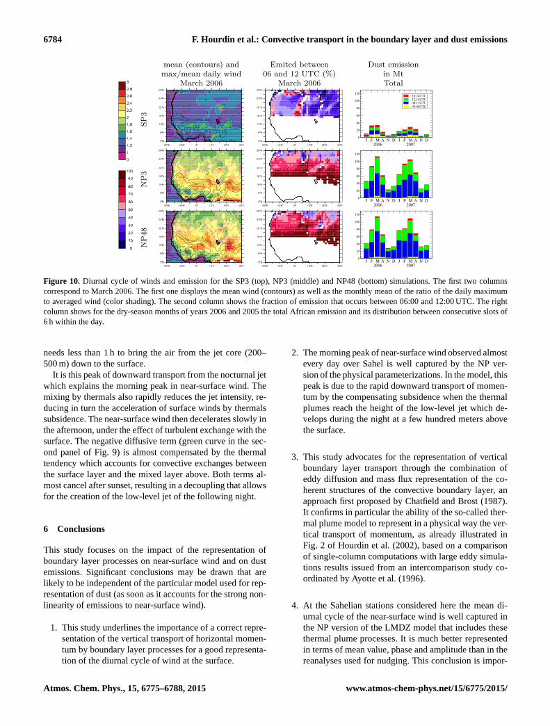
Figure 10. Diurnal cycle of winds and emission for the SP3 (top), NP3 (middle) and NP48 (bottom) simulations. The first two columns

correspond to March 2006. The first one displays the mean wind (contours) as well as the monthly mean of the ratio of the daily maximum

to averaged wind (color shading). The second column shows the fraction of emission that occurs between 06:00 and 12:00 UTC. The right

column shows for the dry-season months of years 2006 and 2005 the total African emission and its distribution between consecutive slots of

6 h within the day.

needs less than 1 h to bring the air from the jet core (200–

500 m) down to the surface.

It is this peak of downward transport from the nocturnal jet

which explains the morning peak in near-surface wind. The

mixing by thermals also rapidly reduces the jet intensity, re-

ducing in turn the acceleration of surface winds by thermals

subsidence. The near-surface wind then decelerates slowly in

the afternoon, under the effect of turbulent exchange with the

surface. The negative diffusive term (green curve in the sec-

ond panel of Fig. 9) is almost compensated by the thermal

tendency which accounts for convective exchanges between

the surface layer and the mixed layer above. Both terms al-

most cancel after sunset, resulting in a decoupling that allows

for the creation of the low-level jet of the following night.

6 Conclusions

This study focuses on the impact of the representation of

boundary layer processes on near-surface wind and on dust

emissions. Significant conclusions may be drawn that are

likely to be independent of the particular model used for rep-

resentation of dust (as soon as it accounts for the strong non-

linearity of emissions to near-surface wind).

1. This study underlines the importance of a correct repre-

sentation of the vertical transport of horizontal momen-

tum by boundary layer processes for a good representa-

tion of the diurnal cycle of wind at the surface.

2. The morning peak of near-surface wind observed almost

every day over Sahel is well captured by the NP ver-

sion of the physical parameterizations. In the model, this

peak is due to the rapid downward transport of momen-

tum by the compensating subsidence when the thermal

plumes reach the height of the low-level jet which de-

velops during the night at a few hundred meters above

the surface.

3. This study advocates for the representation of vertical

boundary layer transport through the combination of

eddy diffusion and mass flux representation of the co-

herent structures of the convective boundary layer, an

approach first proposed by Chatfield and Brost (1987).

It confirms in particular the ability of the so-called ther-

mal plume model to represent in a physical way the ver-

tical transport of momentum, as already illustrated in

Fig. 2 of Hourdin et al. (2002), based on a comparison

of single-column computations with large eddy simula-

tions results issued from an intercomparison study co-

ordinated by Ayotte et al. (1996).

4. At the Sahelian stations considered here the mean di-

urnal cycle of the near-surface wind is well captured in

the NP version of the LMDZ model that includes these

thermal plume processes. It is much better represented

in terms of mean value, phase and amplitude than in the

reanalyses used for nudging. This conclusion is impor-

Atmos. Chem. Phys., 15, 6775–6788, 2015 www.atmos-chem-phys.net/15/6775/2015/

F. Hourdin et al.: Convective transport in the boundary layer and dust emissions 6785

tant for many chemical transport models which rely on

reanalyses for the computation of near-surface winds.

5. An important practical consequence of this point is that

it could be better to use much larger time constants for

nudging than what was currently believed. The ratio-

nale for using time constants of a few hours was to let

the rapid processes represented in turbulent parameter-

izations to express themselves, without departing from

the observed synoptic situation. The problem is that the

time constants which prevail for the creation and con-

trol of the nocturnal jet are typically those of the diur-

nal cycle itself. So constants larger than 1 day should

be used for this particular problem. It seems that with

time constants as large as 48 h the synoptic situation

is still rather well constrained, which probably points

to a reasonable behavior of the physics of the LMDZ

model which does not tend to depart too fast from the

observed situation. Note that the mean diurnal cycle is

almost identical when simulations are conducted with-

out nudging, i.e., in free climate mode (not shown).

Although the detailed analysis of the diurnal cycle of wind

was conducted at the stations for which we have observa-

tions, located at the south of the emission zone, the same

difference among the SP3, NP3 and NP48 simulations is ob-

tained everywhere over the Sahel and Sahara and for all the

winter period, as illustrated in Fig. 10. The left panels show,

for March 2006, the monthly mean of the ratio of the daily

maximum to the daily average of the 10 m wind. This mean

ratio is maximum over Sahel for all simulations. At 12N, it

is typically of 1.6 in SP3 and 2.3 for NP3 and NP48. Over

the Sahara, in the main emission zones, it is of the order of

1.3 for SP3 and 1.8 to 2.2 for NP3 and NP48. The ratio is

systematically a little bit larger for NP48 than for NP3. The

mean wind itself is generally smaller in NP3 than in SP3 and

a little bit stronger in NP48 than in NP3.

As a consequence of the different representation of the

wind diurnal cycle, a much larger fraction of the dust emis-

sions occurs in the morning between 06:00 and 12:00 UTC

in NP3 than in SP3, as seen in the second column of Fig. 10.

This fraction is larger than 90 % in the northern part of Sa-

hara and is slightly larger as well in the NP48 than in the NP3

simulation.

This behavior is not specific to this particular month, as

can be seen on the third column that shows, for all the dry-

season months of years 2006 and 2007, the total emission

over Africa split into slots of 6 h. The dominance of morning

emissions concerns all the months. This figures can be com-

pared with Fig. 4 of Tegen et al. (2013) that shows that more

than 95 % of dust source activation computed from MSG

satellite observations occurs between 06:00 and 12:00 UTC.

By cumulating emissions over the 12 months displayed,

the total emission is 205 Mt for SP3, 757 for NP3 and 765 for

NP48, and the fraction of this emission that occurs between

06:00 and 12:00 UTC is 32, 55 and 61 %, respectively.

Despite a reasonable representation of the near-surface

winds (at least at the stations available, which unfortunately

are not in the main emission zones), and the use of a Weibull

distribution to account for the effect of spatial inhomo-

geneities of wind speed within a grid mesh, the model un-

derestimates the observed dust typically by 20–50 % for the

NP48 simulation that shows the strongest emissions. The

underestimation is similar when considering either AOD or

PM10 concentrations. AOD is sensitive to the atmospheric

column with a stronger contribution of small particles while

the PM10 concentration is a direct measurement of the mass

concentration close to the surface. The fact that both indicate

a similar underestimation suggests a general underestimation

of emissions rather than a size distribution effect.

Such discrepancies are, however, not that exceptional for

simulations of African desert dust (e.g., Todd et al., 2008).

This underestimation does not alter the main result of the

paper, which is that an accurate representation of the diur-

nal evolution of the boundary layer and transport of momen-

tum by boundary layer convective cells must be taken into

account for a good representation of winds. Such a repre-

sentation can be obtained through a combination of turbu-

lent diffusion and mass flux parameterization of the boundary

layer convection. This study also underlines the importance

of in situ long-term and high-frequency meteorological and

dust observations for evaluation and improvement of weather

forecast and climate models.

Acknowledgements. We thank Bernadette Chatenet, the technical

PI of the Sahelian stations from 2006 to 2012, Jean-Louis Rajot,

the scientific co-PI, and the African technicians who manage the

stations: M. Coulibaly and I. Koné from the Institut d’Economie

Rurale in Cinzana, Mali, and A. Maman and A. Zakou from the

Institut de Recherche pour le Développement, Niamey, Niger. The

work was partially supported by the Escape and Acasis project of

the French “Agence Nationale de la Recherche”.

Edited by: Y. Balkanski

References

Alfaro, S. C. and Gomes, L.: Modeling mineral aerosol production

by wind erosion: emission intensities and aerosol size distribu-

tion in source areas, J. Geophys. Res., 106, 18075–18084, 2001.

Angevine, W. M., Jiang, H., and Mauritsen, T.: Performance of an

eddy diffusivity-mass flux scheme for shallow cumulus boundary

layers, Mon. Weather Rev., 138, 2895–2912, 2010.

Ayotte, K. W., Sullivan, P. P., Andrén, A., Doney, S. C., Holt-

slag, A. A., Large, W. G., McWilliams, J. C., Moeng, C.-N.,

Otte, M. J., Tribbia, J. J., and Wyngaard, J. C.: An evaluation of

neutral and convective planetary boundary-layer parameteriza-

tions relative to large eddy simulations, Bound.-Lay. Meteorol.,

79, 131–175, 1996.

Bain, C. L., Parker, D. J., Taylor, C. M., Kergoat, L., and

Guichard, F.: Observations of the Nocturnal Boundary Layer As-

www.atmos-chem-phys.net/15/6775/2015/ Atmos. Chem. Phys., 15, 6775–6788, 2015

6786 F. Hourdin et al.: Convective transport in the boundary layer and dust emissions

sociated with the West African Monsoon, Mon. Weather Rev.,

138, 3142–3156, doi:10.1175/2010MWR3287.1, 2010.

Beljaars, A. C. M. and Viterbo, P.: The sensitivity of win-

ter evaporation to the formulation of aerodynamic resistance

in the ECMWF model, Bound.-Lay. Meteorol., 71, 135–149,

doi:10.1007/BF00709223, 1994.

Cakmur, R. V., Miller, R. L., and Torres, O.: Incorporating the

effect of small-scale circulations upon dust emission in an at-

mospheric general circulation model, J. Geophys. Res., 109,

D07201, doi:10.1029/2003JD004067, 2004.

Callot, Y., Marticorena, B., and Bergametti, G.: Geomorphologic

approach for modelling the surface features of arid environ-

ments in a model of dust emissions: application to the Sa-

hara desert, Geodin. Acta., 13, 245–270, doi:10.1016/S0985-

3111(00)01044-5, 2000.

Chatfield, R. B. and Brost, R. A.: A two-stream model of the

vertical transport of trace species in the convective boundary

layer, J. Geophys. Res., 92, 13263–13276, 1987.

Coindreau, O., Hourdin, F., Haeffelin, M., Mathieu, A., and Rio, C.:

A global climate model with strechable grid and nudging: a tool

for assesment of physical parametrizations, Mon. Weather Rev.,

135, 1474–1489, 2007.

Cuesta, J., Marsham, J. H., Parker, D. J., and Flamant, C.: Dynami-

cal mechanisms controlling the vertical redistribution of dust and

the thermodynamic structure of the West Saharan atmospheric

boundary layer during summer, Atmos. Sci. Lett., 10, 34–42,

doi:10.1002/asl.207, 2009.

Deardorff, J. W.: Preliminary results from numerical integrations of

the unstable planetary boundary layer, J. Atmos. Sci., 27, 1209–

1211, 1970.

Deardorff, J. W.: Theoretical expression for the countergradient ver-

tical heat flux, J. Geophys. Res., 77, 5900–5904, 1972.

Dufresne, J.-L., Foujols, M.-A., Denvil, S., Caubel, A., Marti, O.,

Aumont, O., Balkanski, Y., Bekki, S., Bellenger, H., Benshila, R.,

Bony, S., Bopp, L., Braconnot, P., Brockmann, P., Cadule, P.,

Cheruy, F., Codron, F., Cozic, A., Cugnet, D., de Noblet, N.,

Duvel, J.-P., Ethé, C., Fairhead, L., Fichefet, T., Flavoni, S.,

Friedlingstein, P., Grandpeix, J.-Y., Guez, L., Guilyardi, E.,

Hauglustaine, D., Hourdin, F., Idelkadi, A., Ghattas, J., Jous-

saume, S., Kageyama, M., Krinner, G., Labetoulle, S., Lahel-

lec, A., Lefebvre, M.-P., Lefevre, F., Levy, C., Li, Z. X., Lloyd, J.,

Lott, F., Madec, G., Mancip, M., Marchand, M., Masson, S.,

Meurdesoif, Y., Mignot, J., Musat, I., Parouty, S., Polcher, J.,

Rio, C., Schulz, M., Swingedouw, D., Szopa, S., Talandier, C.,

Terray, P., Viovy, N., and Vuichard, N.: Climate change projec-

tions using the IPSL-CM5 Earth System Model: from CMIP3

to CMIP5, Clim. Dynam., 40, 2123–2165, doi:10.1007/s00382-

012-1636-1, 2013.

Engelstaedter, S., Tegen, I., and Washington, R.: North African

dust emissions and transport, Earth-Sci. Rev., 79, 73–100,

doi:10.1016/j.earscirev.2006.06.004, 2006.

Fiedler, S., Schepanski, K., Heinold, B., Knippertz, P., and Tegen, I.:

Climatology of nocturnal low-level jets over North Africa

and implications for modeling mineral dust emission, J. Geo-

phys. Res., 118, 6100–6121, doi:10.1002/jgrd.50394, 2013.

Forêt, G., Bergametti, G., Dulac, F., and Menut, L.: An optimized

particle size bin scheme for modeling mineral dust aerosol, J.

Geophys. Res., 111, D17310, doi:10.1029/2005JD006797, 2006.

Gillette, D. A.: Fine Particulate emissions due to wind erosion,

Trans. Am. Soc. Agric. Engrs., 20, 890–987, 2003.

Gounou, A., Guichard, F., and Couvreux, F.: Observations of diur-

nal cycles over a West African meridional transect: pre-monsoon

and full-monsoon seasons, Bound.-Lay. Meteorol., 144, 329–

357, doi:10.1007/s10546-012-9723-8, 2012.

Gomes, L., Rajot, J. L., Alfaro, S. C., and Gaudichet, A.: Valida-

tion of a dust production model from measurements performed

in semi-arid agricultural areas of Spain and Niger, Catena, 52,

257–271, doi:10.1016/S0341-8162(03)00017-1, 2003.

Grandpeix, J. and Lafore, J.: A density current parameterization

coupled with Emanuel’s convection scheme, Part I: The models,

J. Atmos. Sci., 67, 881–897, doi:10.1175/2009JAS3044.1, 2010.

Guichard, F., Kergoat, L., Mougin, E., Timouk, F., Baup, F., Hi-

ernaux, P., and Lavenu, F.: Surface thermodynamics and radia-

tive budget in the Sahelian Gourma: Seasonal and diurnal cycles,

J. Hydrol., 375, 161–177, doi:10.1016/j.jhydrol.2008.09.007,

2009.

Holben, B. N., Tanre, D., Smirnov, A., Eck, T. F., Slutsker, I.,

Abuhassan, N., Newcomb, W. W., Schafer, J., Chatenet, B.,

Lavenu, F., Kaufman, Y., Van de Castle, J., Setzer, A.,

Markham, B., Clark, D., Frouin, R., Halthore, R., Karnieli, A.,

O’Neill, N. T., Pietras, C., Pinker, R. T., Voss, K., and Zi-

bordi, G.: An emerging ground-based aerosol climatology:

Aerosol Optical Depth from AERONET, J. Geophys. Res., 106,

12067–12098, 2001.

Holtslag, A. A. M. and Boville, B. A.: Local versus non-local

boundary-layer diffusion in a global climate model, J. Climate,

6, 1825–1842, 1993.

Hourdin, F., Couvreux, F., and Menut, L.: Parameterisation of the

dry convective boundary layer based on a mass flux representa-

tion of thermals, J. Atmos. Sci., 59, 1105–1123, 2002.

Hourdin, F., Foujols, M.-A., Codron, F., Guemas, V., Dufresne, J.-

L., Bony, S., Denvil, S., Guez, L., Lott, F., Ghattas, J., Bracon-

not, P., Marti, O., Meurdesoif, Y., and Bopp, L.: Impact of the

LMDZ atmospheric grid configuration on the climate and sen-

sitivity of the IPSL-CM5A coupled model, Clim. Dynam., 40,

2167–2192, doi:10.1007/s00382-012-1411-3, 2013a.

Hourdin, F., Grandpeix, J.-Y., Rio, C., Bony, S., Jam, A., Cheruy, F.,

Rochetin, N., Fairhead, L., Idelkadi, A., Musat, I., Dufresne, J.-

L., Lahellec, A., Lefebvre, M.-P., and Roehrig, R.: LMDZ5B: the

atmospheric component of the IPSL climate model with revisited

parameterizations for clouds and convection, Clim. Dynam., 40,

2193–2222, doi:10.1007/s00382-012-1343-y, 2013b.

Jam, A., Hourdin, F., Rio, C., and Couvreux, F.: Resolved ver-

sus parametrized boundary-layer plumes, Part III: Derivation of

a statistical scheme for cumulus clouds, Bound.-Lay. Meteorol.,

147, 421–441, doi:10.1007/s10546-012-9789-3, 2013.

Knippertz, P. and Todd, M. C.: Mineral dust aerosols over the

Sahara: meteorological controls on emission and transport

and implications for modeling, Rev. Geophys., 50, RG1007,

doi:10.1029/2011RG000362, 2012.

Laurent, B., Marticorena, B., Bergametti, G., Léon, J. F., and Ma-

howald, N. M.: Modeling mineral dust emissions from the Sahara

desert using new surface properties and soil database, J. Geo-

phys. Res., 113, D14218, doi:10.1029/2007JD009484, 2008.

Largeron, Y., Guichard, F., Bouniol, D., Couvreux, F., Ker-

goat, L., and Marticorena, B.: Can we use surface wind

fields from meteorological reanalyses for Sahelian dust emis-

Atmos. Chem. Phys., 15, 6775–6788, 2015 www.atmos-chem-phys.net/15/6775/2015/

F. Hourdin et al.: Convective transport in the boundary layer and dust emissions 6787

sion simulations?, Geophys. Res. Lett., 42, 2490–2499,

doi:10.1002/2014GL062938, 2015.

Lothon, M., Saïd, F., Lohou, F., and Campistron, B.: Observation

of the diurnal cycle in the low troposphere of West Africa, Mon.

Weather Rev., 136, 3477, doi:10.1175/2008MWR2427.1, 2008.

Marticorena, B. and Bergametti, G.: Modeling the atmospheric dust

cycle: 1 Design of a soil derived dust production scheme, J. Geo-

phys. Res., 100, 16415–16430, 1995a.

Marticorena, B. and Bergametti, G.: Modeling the atmospheric

dust cycle: design of a soil-derived emission scheme, J. Geo-

phys. Res., 102, 16415–16430, 1995b.

Marticorena, B., Bergametti, G., Aumont, B., Callot, Y.,

N’doumé, C., and Legrand, M.: Modeling the atmospheric dust

cycle: 2. Simulation of Saharan dust sources, J. Geophys. Res.,

102, 4387–4404, doi:10.1029/96JD02964, 1997.

Marticorena, B., Chatenet, B., Rajot, J. L., Traoré, S., Coulibaly,

M., Diallo, A., Koné, I., Maman, A., NDiaye, T., and Zakou, A.:

Temporal variability of mineral dust concentrations over West

Africa: analyses of a pluriannual monitoring from the AMMA

Sahelian Dust Transect, Atmos. Chem. Phys., 10, 8899–8915,

doi:10.5194/acp-10-8899-2010, 2010.

Menut, L., Schmechtig, C., and Marticorena, B.: Sensitivity of the

sandblasting fluxes calculations to the soil size distribution accu-

racy, J. Atmos. Ocean. Tech., 22, 1875–1884, 2005.

Menut, L., Foret, G., and Bergametti, G.: Sensitivity of mineral dust

concentrations to the model size distribution accuracy, J. Geo-

phys. Res.-Atmos., 112, D10210, doi:10.1029/2006JD007766,

2007.

Menut, L., Chiapello, I., and Moulin, C.: Previsibility of min-

eral dust concentrations: the CHIMERE-DUST forecast during

the first AMMA experiment dry season, J. Geophys. Res., 114,

D07202, doi:10.1029/2008JD010523, 2009.

Menut, L., Bessagnet, B., Khvorostyanov, D., Beekmann, M.,

Blond, N., Colette, A., Coll, I., Curci, G., Foret, G., Hodzic,

A., Mailler, S., Meleux, F., Monge, J.-L., Pison, I., Siour, G.,

Turquety, S., Valari, M., Vautard, R., and Vivanco, M. G.:

CHIMERE 2013: a model for regional atmospheric composition

modelling, Geosci. Model Dev., 6, 981–1028, doi:10.5194/gmd-

6-981-2013, 2013.

Moulin, C., Gordon, H. R., Banzon, V. F., and Evans, R. H.:

Assessment of Saharan dust absorption in the visible

from SeaWiFS imagery, J. Geophys. Res., 106, 18239,

doi:10.1029/2000JD900812, 2001.

Neggers, R. A. J.: A dual mass flux framework for boundary layer

convection, Part II: Clouds, J. Atmos. Sci., 66, 1489–1506, 2009.

Neggers, R. A. J., Köhler, M., and Beljaars, A. C. M.: A dual mass

flux framework for boundary layer convection. Part I: Trans-

port, J. Atmos. Sci., 66, 1465, doi:10.1175/2008JAS2635.1,

2009.

Nickling, W. G. and Gillies, J. A.: Emission of fine-grained par-

ticulates from desert soils, in Paleoclimatology and Paleometeo-

rology: Modern and Past Patterns of Global Atmospheric Trans-

port, edited by: Leinen, M. and Sarnthein, M., Kluwer Academic

Publ., Dordrecht, 133–165, 1989.

Nickling, W. G. and Gillies, J. A.: Dust emission and transport in

Mali, West Africa, Sedimentology, 40, 859–868, 1993.

Parker, D. J., Burton, R. R., Diongue-Niang, A., Ellis, R. J., Fel-

ton, M., Taylor, C. M., Thorncroft, C. D., Bessemoulin, P.,

and Tompkins, A. M.: The diurnal cycle of the West African

monsoon circulation, Q. J. Roy. Meteor. Soc., 131, 2839–2860,

doi:10.1256/qj.04.52, 2005.

Pergaud, J., Masson, V., Malardel, S., and Couvreux, F.: A param-

eterization of dry thermals and shallow cumuli for mesoscale

numerical weather prediction, Bound.-Lay. Meteorol., 132, 83–

106, doi:10.1007/s10546-009-9388-0, 2009.

Rajot, J. L., Alfaro, S. C., Gomes, L., and Gaudichet, A.: Soil crust-

ing on sandy soils and its influence on wind erosion, Catena, 53,

1–16, 2003.

Redelsperger, J.-L., Thorncroft, C. D., Diedhiou, A., Lebel, T.,

Parker, D. J., and Polcher, J.: African monsoon multidisciplinary

analysis: an international research project and field campaign, B.

Am. Meteorol. Soc., 87, 1739–1746, doi:10.1175/BAMS-87-12-

1739, 2006.

Rio, C. and Hourdin, F.: A thermal plume model for the convective

boundary layer: representation of cumulus clouds, J. Atmos. Sci.,

65, 407–425, 2008.

Rio, C., Hourdin, F., Grandpeix, J., and Lafore, J.: Shifting the di-

urnal cycle of parameterized deep convection over land, Geo-

phys. Res. Lett., 36, L07809, doi:10.1029/2008GL036779, 2009.

Rio, C., Hourdin, F., Couvreux, F., and Jam, A.: Resolved versus

parametrized boundary-layer plumes, Part II: Continuous formu-

lations of mixing rates for mass-flux schemes, Bound.-Lay. Me-

teorol., 135, 469–483, doi:10.1007/s10546-010-9478-z, 2010.

Schepanski, K., Tegen, I., Todd, M. C., Heinold, B., BöNisch, G.,

Laurent, B., and Macke, A.: Meteorological processes forcing

Saharan dust emission inferred from MSG-SEVIRI observations

of subdaily dust source activation and numerical models, J. Geo-

phys. Res.-Atmos., 114, D10201, doi:10.1029/2008JD010325,

2009.

Schmechtig, C., Marticorena, B., Chatenet, B., Bergametti, G., Ra-

jot, J. L., and Coman, A.: Simulation of the mineral dust content

over Western Africa from the event to the annual scale with the

CHIMERE-DUST model, Atmos. Chem. Phys., 11, 7185–7207,

doi:10.5194/acp-11-7185-2011, 2011.

Seinfeld, J. H. and Pandis, S. N. (Eds.): Atmospheric Chemistry and

Physics: From Air Pollution to Climate Change, in: Atmospheric

chemistry and physics: from air pollution to climate change, New

York, NY: Wiley, 1998 Physical description: xxvii, 1326 pp.,

Wiley-Interscience Publication, ISBN: 0471178152, 1998.

Shao, Y. and Lu, I.: A simple expression for wind erosion threshold

friction velocity, J. Geophys. Res., 105, 22437–22443, 2000.

Shao, Y., Ishizuka, M., Mikami, M., and Leys, J. F.: Pa-

rameterization of size-resolved dust emission and valida-

tion with measurements, J. Geophys. Res., 116, D08203,

doi:10.1029/2010JD014527, 2011.

Siebesma, A. P., Soares, P. M. M., and Teixeira, J.: A combined

eddy-diffusivity mass-flux approach for the convective boundary

layer, J. Atmos. Sci., 64, 1230, doi:10.1175/JAS3888.1, 2007.

Slingo, A., Ackerman, T. P., Allan, R. P., Kassianov, E. I., Mc-

Farlane, S. A., Robinson, G. J., Barnard, J. C., Miller, M. A.,

Harries, J. E., Russell, J. E., and Dewitte, S.: Observations

of the impact of a major Saharan dust storm on the atmo-

spheric radiation balance, Geophys. Res. Lett., 33, L24817,

doi:10.1029/2006GL027869, 2006.

Soares, P. M. M., Miranda, P. M. A., Siebesma, A. P., and Teix-

eira, J.: An eddy-diffusivity/mass-flux parametrization for dry

and shallow cumulus convection, Q. J. Roy. Meteor. Soc., 130,

3365–3383, 2004.

www.atmos-chem-phys.net/15/6775/2015/ Atmos. Chem. Phys., 15, 6775–6788, 2015

6788 F. Hourdin et al.: Convective transport in the boundary layer and dust emissions

Solmon, F., Mallet, M., Elguindi, N., Giorgi, F., Zakey, A.,

and Konaré, A.: Dust aerosol impact on regional pre-

cipitation over western Africa, mechanisms and sensitivity

to absorption properties, Geophys. Res. Lett., 35, L24705,

doi:10.1029/2008GL035900, 2008.

Sow, M., Alfaro, S. C., Rajot, J. L., and Marticorena, B.: Size re-

solved dust emission fluxes measured in Niger during 3 dust

storms of the AMMA experiment, Atmos. Chem. Phys., 9, 3881–

3891, doi:10.5194/acp-9-3881-2009, 2009.

Spyrou, C., Kallos, G., Mitsakou, C., Athanasiadis, P., Kalogeri, C.,

and Iacono, M. J.: Modeling the radiative effects of desert dust

on weather and regional climate, Atmos. Chem. Phys., 13, 5489–

5504, doi:10.5194/acp-13-5489-2013, 2013.

Stull, R. B.: Transilient turbulence theory, Part I: The concept of

eddy-mixing across finite distances, J. Atmos. Sci., 41, 3351–

3367, 1984.

Taylor, K. E., Stouffer, R. J., and Meehl, G. A.: An overview of

CMIP5 and the experiment design, B. Am. Meteorol. Soc., 93,

485–498, doi:10.1175/BAMS-D-11-00094.1, 2012.

Tegen, I., Schepanski, K., and Heinold, B.: Comparing two years

of Saharan dust source activation obtained by regional modelling

and satellite observations, Atmos. Chem. Phys., 13, 2381–2390,

doi:10.5194/acp-13-2381-2013, 2013.

Tiedtke, M.: A comprehensive mass flux scheme for cumulus pa-

rameterization in large-scale models, Mon. Weather Rev., 117,

1179–1800, 1989.

Todd, M. C., Bou Karam, D., Cavazos, C., Bouet, C., Heinold, B.,

Baldasano, J. M., Cautenet, G., Koren, I., Perez, C., Solmon, F.,

Tegen, I., Tulet, P., Washington, R., and Zakey, A.: Quanti-

fying uncertainty in estimates of mineral dust flux: an inter-

comparison of model performance over the Bodélé Depres-

sion, northern Chad, J. Geophys. Res.-Atmos., 113, D24107,

doi:10.1029/2008JD010476, 2008.

Troen, I. and Mahrt, L.: A simple model of the atmospheric bound-

ary layer: sensitivity to surface evaporation, Bound.-Lay. Meteo-

rol., 37, 129–148, 1986.

Yamada, T.: Simulations of nocturnal drainage flows by a q2l tur-

bulence closure model, J. Atmos. Sci., 40, 91–106, 1983.

Yoshioka, M., Mahowald, N. M., Conley, A. J., Collins, W. D., Fill-

more, D. W., Zender, C. S., and Coleman, D. B.: Impact of desert

dust radiative forcing on sahel precipitation: relative importance

of dust compared to sea surface temperature variations, vegeta-

tion changes, and greenhouse gas warming, J. Climate, 20, 1445,

doi:10.1175/JCLI4056.1, 2007.

Atmos. Chem. Phys., 15, 6775–6788, 2015 www.atmos-chem-phys.net/15/6775/2015/