parametric and optimal design of modular machine tools
TRANSCRIPT

PARAMETRIC AND OPTIMAL DESIGN OF MODULAR MACHINE TOOLS
A Dissertation
Presented to
The Faculty of the Graduate School
University of Missouri – Columbia
In Partial Fulfillment
Of the Requirements for the Degree
Doctor of Philosophy
By
Donald Harby
Dr. Yuyi Lin, Dissertation Supervisor
December 2007

The undersigned, appointed by the dean of the Graduate School, have examined the dissertation entitled
PARAMETRIC AND OPTIMAL DESIGN OF MODULAR MACHINE TOOLS
presented by Donald Harby,
a candidate for the degree of doctor of philosophy,
and hereby certify that, in their opinion, it is worthy of acceptance.
Professor Yuyi Lin
Professor Douglas Smith
Professor Robert Winholtz
Professor A. Sherif El-Gizawy
Professor Luis Occena

ii
ACKNOWLEDGMENTS
The author is deeply indebted to his advisor, Dr. Yuyi Lin, for his
invaluable direction and assistance. He further extends many thanks to the
members of his doctoral committee, Dr. Douglas Smith, Dr. Sherif El-Gizawy, Dr.
Robert Winholtz, and Dr. Luis Occena, for their time and effort in reading the
manuscript and their many helpful suggestions.
The author would also like to express his appreciation to Dr. Douglas
Smith, for the GAANN fellowship, without this support this project would not have
been possible. The author would also like to express his appreciation to Dr.
Robert Kallenbach for the use of the computer hardware and software and his
valuable input on the topic of Neural Networks.
Finally and most importantly, the author wishes to acknowledge the
support and encouragement of my parents, as well as my wife and children,
Denee, Weston, and Wyatt, for their loving support and personal sacrifices. The
author would like to dedicate this work to them.

iii
TABLE OF CONTENTS
LIST OF FIGURES ............................................................................................... v
LIST OF TABLES ............................................................................................... viii
CHAPTER 1 INTRODUCTION ............................................................................. 1
1.1 Background, Motivation and Purpose ........................................................ 1
1.2 Literature Review ........................................................................................ 4
1.2.1 Discrete Optimization ........................................................................... 4
1.2.2 Heuristic Discrete Optimization Methods in Mechanical Sturctures ...... 6
1.2.3 Particle Swarm Optimization ............................................................... 8
1.2.4 Surrogate Modeling ........................................................................... 10
1.2.5 Structural Optimization ...................................................................... 12
1.3 Objective .................................................................................................. 15
CHAPTER 2 THEORETICAL BACKGROUND ................................................... 17
2.1 Finite Element Analysis ............................................................................ 17
2.2 High-Speed FEA Approximation .............................................................. 26
2.3 Basic NN Structure .................................................................................. 27
2.4 NN Test .................................................................................................... 33
2.6 NN training ............................................................................................... 45

iv
2.7 General Comments and Results from NN test ......................................... 51
2.7 Optimization Algorithms ........................................................................... 52
2.8 Branch and Bound Discrete Optimization ................................................ 54
2.9 Hybrid Continuous Optimization ............................................................... 61
CHAPTER 3 DISCREET OPTIMIZATION OF MMT STRUCTURES ................. 66
3.1 Application of DSO, FEA, and NN ............................................................ 66
3.2 Traditional Topology Optimization ............................................................ 74
3.3 Large Scale MMT Base Optimization ....................................................... 83
CHAPTER 4 CONCLUSTION AND FUTURE WORK ........................................ 87
4.1 Conclusion ............................................................................................... 87
4.2 Future Research ...................................................................................... 88
REFERENCES ................................................................................................... 90
APPENDIX ......................................................................................................... 98
Appendix A: MATLAB FEA Functions ............................................................ 98
Appendix B: MATLAB Program Used to Test FEA Approximation .............. 102
Appendix C: MATLAB Program For DSO of Typical MMT Base Side.......... 116
Appendix D: MATLAB Program – Material Distribution Topology Optimization
...................................................................................................................... 131
Appendix E: MATLAB Program PSO of MMT Base 3D ............................... 136
Appendix F: MATLAB Program Used to Generate AutoLISP Program ........ 149
Appendix G: Sample AutoLISP Code Generated from MATLAB ................. 151
VITA ................................................................................................................. 157

v
LIST OF FIGURES
Figure 1 Typical MMT structure (ASME B5.43M) ................................................. 2
Figure 2. Typical grounded structure ................................................................. 14
Figure 3. Standard steel S and C profiles .......................................................... 15
Figure 4. General Beam .................................................................................... 18
Figure 5. ............................................................................................................. 20
(a) The free-body diagram .................................................................................. 20
(b) the first element ............................................................................................. 20
Figure 6. A typical neuron .................................................................................. 28
Figure 7. Transfer functions ............................................................................... 29
Figure 8. A typical 2 layer feed forward neural network ..................................... 30
Figure 9. Neural network training flowchart ....................................................... 31
Figure 10. Typical radial bias neuron ................................................................. 32
Figure 11. Test cantilever beam ........................................................................ 33
Figure 12. Simple beam nodal deflection. ........................................................ 35
Figure 13. Modified simple beam nodal deflection. ............................................ 36
Figure 14. NN training with no previous weights and biases. ............................ 37
Figure 15. Training using previous weights and biases. .................................... 38
Figure 16 Side of typical MMT base structure ................................................... 39
Figure 17. Training time with no previous weights and biases........................... 41
Figure 18. Modified structure topography .......................................................... 42
Figure 19. Time to retrain NN ............................................................................ 44
vi
Figure 20. Training history for traingda .............................................................. 47
Figure 21. Training history for trainrp ................................................................. 48
Figure 22. Training history for trainscg .............................................................. 49
Figure 23. Training history for trainlm ................................................................ 50
Figure 24. Structural Bracket Example .............................................................. 55
Figure 25. Branch and Bound Tree for the Structural Bracket Example ............ 57
Figure 26. Tree for typical MMT base side ........................................................ 60
Figure 27. Branch and bound flowchart for MMT base side .............................. 60
Figure 28. Typical topology and cross section ................................................... 61
Figure 29. Particle swarm optimizer flowchart ................................................... 65
Figure 30. Parallel NN training and branch and bound ...................................... 69
Figure 31. Optimal topology for first load condition ............................................ 70
Figure 32. Optimal design for second load location ........................................... 71
Figure 33. Optimal design for third load location ............................................... 72
Figure 34. Optimal design for fourth load location ............................................. 73
Figure 35. Optimal topology using material density method .............................. 74
Figure 36. Optimal topology using material distrubution method ....................... 79
Figure 37. Discrete optimization using NN with lateral load ............................... 81
Figure 38. Discrete optimization using the material density method and 25%
volume ................................................................................................................ 82
Figure 39. Discrete optimization using the material density method and 30%
volume ................................................................................................................ 82

vii
Figure 40. Discrete optimization using the material density method and 40%
volume ................................................................................................................ 82
Figure 41. Discrete optimization using the material density method and 50%
volume ................................................................................................................ 83
Figure 42. The optimal topology with applied loads ........................................... 85
Figure 43. Program generated 3D model .......................................................... 86

viii
LIST OF TABLES
Table 1. Standard steel cross sections ...................................................................... 14
Table 2. Simple cantilever beam example displacements and CPU times ......... 34
Table 3. Modified simple cantilever beam example displacements and CPU
times ................................................................................................................................. 36
Table 4. Nodal displacement and CPU time ............................................................. 40
Table 5. Standard steel shapes .................................................................................. 40
Table 6. Displacements and CPU times for structure with new topology ............ 43
Table 7. Standard steel shapes .................................................................................. 43
Table 8. Optimization results for first load condition ................................................ 70
Table 9. Optimization results for second load condition ......................................... 72
Table 10. Optimization results for third load condition ............................................ 72
Table 11. Optimization results for forth load condition ............................................ 73
Table 12. Element sections and CPU times for 3D MMT base ............................. 84

1
CHAPTER 1
INTRODUCTION
1.1 Background, Motivation and Purpose
Current manufacturing enterprises are faced with more competition than
ever. To survive and flourish in the global market manufacturers are constantly
looking for ways to increase production rate and lower cost. Machine tools are
used in many modern manufacturing processes. Design and selection of
machine tools has a great impact on the productivity and cost of many
manufacturing processes. During the past several decades a significant amount
of research has been conducted in the area of machine tool design, with the goal
to develop more efficient and lower cost tools for manufacturing.
Over the years machine tools designed for manufacturing have developed
into two classes. The first is general purpose machine tools designed for a large
range of operations. Examples of these are standard milling machines or lathes.
The design and operation of these standard machines is a very mature subject
and little research is left to be done. The other class of machine tools are those
designed for a very specific part of a process. These machine tools are
sometimes referred to as dedicated machine tools. These types of machine tools
are usually used in high speed or high volume production. The machining of
automotive engine blocks is an example. Many interesting areas of these
specific machine tools can be investigated and improved. This approach is

2
generally very effective; however, it is not without disadvantages. If the product
design is changed even slightly, the machine tool may have to be scrapped and
a new machine tool designed and built. Another problem is that the lead-time to
design and build such a machine can be very long. An approach to overcome
these problems is to produce a re-configurable or modular machine tool (MMT).
Using this approach custom machine tools could be designed and built quickly
from existing modular components (Figure 1).
Figure 1. Typical MMT structure (ASME B5.43M)
There already exist standards for MMT components (ASME B.43M)[1]. Typically,
these MMT components are made of large steel castings or fabrications. Stress,
strain, deflection, and rigidity are not an issue with these components so very
little design effort is put into MMT components. A better approach would be to

3
fabricate these components from stock pieces of standard steel shapes such as
standard steel C or L cross sections. Many standard MMT components could be
quickly assembled from a library of stock components. Due to the rapidly
increasing cost of steel in recent years it would cost much less than cast
components. Also, a significant reduction in cost could be realized by combining
modern optimization and analysis techniques. An automated method of selecting
elements and designing MMT could be developed. The idea of using an
inventory of standard steel cross-section components coupled with optimization
and analysis leads to a very interesting discrete structural optimization (DSO)
problem.
With the fast advances of computer technology, much progress has been
made in DSO research. However, the roots of DSO come from the early non-
linear integer programming research initiatives of the US military, specifically, the
work of the Rand Corporation in the 1950’s and 60’s[2]. The conclusion of most
of this early work on integer and discrete optimization was that the problems
required exponential-time solutions or 2n operations to solve [3]. This led to the
idea that only small scale problems could be solved. With the rapid increase in
computer speed many new approaches to DSO have been proposed. Some of
these areas of research include partial enumeration, genetic algorithms (GA) and
simulated annealing (SA) [4, 5, 6, 7, 8, 9, and 10]. Many of these areas of DSO
are still very immature and should be areas of current research [11]. Many of
these techniques have less than exponential-time solutions.

4
Even if the difficulties of discrete optimization are overcome, many other
areas of DSO, as applied to MMT, need further investigation. Most of the current
research effort has been directed to truss structures or structures with pinned
joints. The stress, strain or displacement constraints in these types of models
can easily be solved using analytical methods. This is fine for most civil
engineering problems, i.e., bridges or buildings; however, for MMT this needs to
be extended to frame and 3D solid components. When the model is extended to
frame or 3D solid components, it is the current accepted practice to use finite
element analysis or methods (FEA or FEM). The use of FEA with DSO has one
major disadvantage in that they are often computationally costly. Because of the
large number of FEA calls in DSO, one of the most important potential areas of
research is finding faster FEA algorithms or alternatives to FEA [11].
1.2 Literature Review
A review of the literature pertaining to discrete structural optimization as
related to this study can be divided into five sections; discrete optimization in
general, heuristic discrete optimization methods in mechanical structures, particle
swarm optimization, surrogate modeling, and structural optimization.
1.2.1 Discrete Optimization
Discrete optimization has been an important area of research over the last
few decades. A wide variety of algorithms have been developed and applied to

5
many areas of mathematics and engineering [12]. Even with extensive research
an efficient and general method of discrete optimization seems difficult to obtain.
In the 1950’s and early 1960’s many methods were tested on discrete
optimization problems. It was generally accepted that most methods except full
enumeration failed to produce a global optimum. But, full enumeration was
impractical to solve anything but trial problems [13]. Land and Doig used non-
linear programming relaxation to determine bounds of a discrete problem. This
first general method for integer programming problems was found to be too
difficult to efficiently implement on computers [14]. Dakin then modified this
method to be efficiently implemented on computers [15]. Algorithms of this type,
those that obtain bounds from relaxation methods and then use the bounds to
prune, are generally referred to as branch and bound algorithms. Little et al. was
the first to use the branch and bound term when appling this type of algorithm to
the traveling salesman problem [16]. Edmonds developed a general purpose
branch and bound algorithm for discrete optimization and he proved it would
solve discrete problems in polynomial time [17]. Most of this early research was
focused on linear well behaved convex problems. Linear programming was the
most accepted relaxation method. However, some later work showed that the
branch and bound method could be extended to non-linear systems by using
non-linear relaxation methods [18]. Over the years other methods of discrete
optimization have been developed. Many of these methods rely on random or
heuristic searches. Roth developed a method of combining random and partial

6
searches [19]. Initial random starting points are generated, then partial searches
were used to find the local optimum. The process is then repeated in an attempt
to find a global optimum. This method was tested successfully on large
problems with modest computational cost. A method that used common features
or details of many discrete optimization problems as a library of optimization
methods was developed by Goldstein and Lesk [20]. This method was adapted
to many problems, however, it was not as good as some heuristic methods. In a
general review of numerical optimization methods More et.al. found the bulk of
the research prior to 1979 had been based on relaxation methods of linear
programming [21]. They also concluded there was room for further research in
discrete optimization, especially using heuristic methods. Most of the previous
research on discrete optimization was based on branch and bound or random
search methods and had been oriented toward special problems and very few
general purpose methods existed [22]. In a recent survey of discrete
optimization Shcherbina concluded that there is doubt that general discrete
optimization problems could be solved efficiently and that the branch and bound
method may be the most practical [23].
1.2.2 Heuristic Discrete Optimization Methods in Mechanical Sturctures
Over the years many methods have been developed to solve discrete
optimization problems in mechanical structures. One of the most popular
approaches in recent years has been the use of heuristic methods. These

7
methods include not only genetic algorithms (GA) and simulated annealing (SA)
but a few lesser known approaches.
The comparison of GA and SA to full enumeration and branch and bound
has been studied by several researchers. Balling used a SA method to optimize
steel frames using a set of standard discrete shapes [24]. This research used
realistic three dimensional test problems and the results were compared to a
modified linear branch and bound method. The results using the SA method
were shown to be similar to the branch and bound method. Kocer and Arora
compared full enumeration, SA, and GA on standard discrete prefabricated steel
sections [25]. The cross-section shape and steel grades were considered as
discrete variables. In this research the GA method found the optimal solution in
all cases and was the most efficient in terms of CPU time. Huang and Arora
compared GA, SA, and full enumeration and concluded, by the use of examples,
that GA and SA could be used to find the global optima [25].
Although the GA and SA methods have received much of attention in
recent years with respect to discrete optimization they have a few areas with
unanswered questions. For instance, will they always produce global optima and
can they be implemented and tuned to solve discrete structural optimization
problems? Using a practical structural system and a GA based method Rajeev
and Krishnamoorthy efficiently solved a discrete variable problem with
constraints [26]. They showed that even though the GA is not well suited for
constrained problems a penalty-based transformation can be implemented. They

8
also showed the GA method is suitable for a parallel computing environment.
Near optimal solutions in reasonable computing times were obtained on large
design space layout and sizing problems of steel roof trusses using a GA by
Koumousis et al. [27]. They also reported that no clear rules exist for tuning of
the GA parameters and the estimate of the parameters is delicate. Using the
uniform building code as constraints Camp et al. developed a GA based method
for optimizing two-dimensional steel frame structures [28]. The method was
tested on 30 designs. The method always produced structures satisfying the
code standards while minimizing the weight but the solution was not guaranteed
to be global. Lu and Kota successfully applied a GA method to a mixed discrete
topology and continuous sizing problem [29]. A new heuristic method based
loosely on the harmonics of music is the harmony search (HS) method. This
method is simple and mathematically less complex than the GA. Its convergence
capability was shown to be better than GA on discrete sizing variable problems
[30]. A common conclusion in the literature with respect to GA and SA is that
they both require considerable user insight and adjustment to the parameters to
get reasonable results [10].
1.2.3 Particle Swarm Optimization
Particle swarm optimization (PSO) is a new huristic based method that
has generated much recent inerest. It is based on the self organizing behavior of
a group with no leaders such as a flock of birds or a school of fish [31 and 32].

9
These groups of individuals have no knowledge of the behavior of the entire
group (global behavior). They only have knowledge about their local
environment, but they can converge and move as a group based on local
individual information. They are capable of complex behavior such as flocking,
homing, exploration, and herding [33, 34, and 35]. Bird flocking [35] and fish
schooling [36] behavior are two of the most studied areas. When applying these
methods to real world optimization problems an effective particle initialization
scheme must be used. Several methods of initiation are presented in the
literature [37, 38, 39, 40, and 41]. These methods are used mainly to ensure that
the search space is uniformly covered. PSO and evolutionary algorithms (EA)
such as GA and SA have many similarities, however, some literature suggests
they should be treated separately [32]. Both methods use a stochastic search
process. PSO does not use the concept of survival of the fittest. Unfit individuals
in the PSO do not die. Also, unlike GA and SA, PSO is not easy to implement for
discrete optimization problems.
The concept of PSO was first introduced by Kennedy and Eberhart [42].
Using a PSO based on swarms or flocks, they optimized non-linear functions.
Kennedy and Eberhart also compared PSO to GA for non-linear function
optimization, neural network learning, and robot task learning [43]. They showed
that PSO is a very simple concept and it can be implemented with just a few lines
of code. Their implementation only used primitive math operations and was also
computationally inexpensive. Song and Gu studied the ability of PSO to find

10
global solutions [44]. Even though PSO is effective, they found there is no
mathematical theory to support that it is a global optimizer. Langdon and Poli
compared and contrasted PSO with a non-standard Newton-raphson based
gradient method [45]. They found that a theoretical analysis of PSO is very
difficult and that we do not have a good mathematical understanding of why PSO
performs better or worse on a problem of a given type. Several researchers
found PSO to perform better in early iterations but that it is not competitive with
other methods when the number of iterations is increased [44, 45, and 47].
In recent years the concept of PSO has been applied to various
engineering problems. Specifically, it has been applied to structural design
optimization problems. Ant colony optimization (ACO), a type of PSO, was
tested on steel frame optimization problems with discrete variables by Camp et al.
[48]. In this research they compared ACO to GA and they found it more effective
and less affected by poor initial solutions. Perez and Behdinan tested PSO on
several well-known structural test problems [49]. The PSO method found better
results on these test problems than any of the other optimization algorithms used
in previous research.
1.2.4 Surrogate Modeling Structural optimization, especially discrete structural optimization of
practical problems, requires low computational cost and accuracy for all of the
processes. By far the most computationally costly process is the FEA. The FEA

11
for large-scale three-dimensional problems and eigenfrequency problems
becomes difficult to optimize practically.
The current literature suggests approximation methods for such large
scale optimization models. Several different methods are reported in this
literature. These include Response Surface Modeling (RSM), Radial Bias,
Neural Network (NN), and Kriging [50-54, and 80].
The kriging model is one of the most popular methods. This method was
originally developed for the mining industry to help model the location of minerals
and gems. Sakata et al. reported good results using kriging methods on large-
scale eigenfrequency problems [51]. The results were comparable with those
from a NN method. One of the most attractive aspects of kriging is that it has the
ability to estimate outputs in areas of the design space that have not been tested
with the FEA [52]. In other words, it is effective at extrapolation as well as
interpolation. The one draw back to kriging is that fitting the data and developing
the model is complex and costly, because it requires an optimization routine. [50
and 52].
Low order polynomial approximations, also known as RSM, are often used
because they are easy to implement and software is readily available [50]. RMS
is often used when experimental data sets are available or when a combination
of experimental and numerical data sets is employed [53]. In [50] it was
concluded that radial bias and kriging methods performed better and were more
accurate on large problems compared to some of the other methods.

12
In this research radial bias and NN were considered to be similar. This is
because they are both modeled after biological systems and because they are in
the same Matlab toolbox and use the same Matlab functions. Most of the
literature found NN to have some of the best performance and most accurate
results [50]. The NN method was even used as a benchmark for other methods
[51]. The only drawbacks are the computational cost to train the network [50, 51,
54, and 55] and the necessity of a skilled operator to setup the network [55].
These drawbacks are easily overcome by using the latest Matlab NN toolbox.
The toolbox makes it easy to setup and train complex NN’s and the speed and
accuracy greatly outweigh the cost of training the network.
1.2.5 Structural Optimization
Over the years three broad approaches to structural topology optimization
have evolved based on grounded structures [11]. One is based on material
homogenization [56] and one on material density [57]. The homogenization and
material density approaches have been the subject of research in recent years
and have few areas left to investigate when applied to DSO [56, 58, and 59].
These two techniques rely on the design space containing a fine mesh of
elements. Voids are created or elements removed through the optimization
process. A discrete structure will emerge from the optimization process.
However, it may be difficult to create a structure of standard set of structural
members using this process. Also, the structure created may not be optimal [11].

13
These two methods are very well suited to cast, molded, or formed parts that
may take on any size or shape.
These methods generally use structural compliance as a constraint.
Cheng and Jiang showed compliance is generally continuous over the feasible
design domain in truss or frame topology problems and it should be considered
as a global constraint. They also showed that stress and buckling constraints are
discontinuous and are local (element) constraints for the same problems [82].
Using the idea of global and local constraints Cheng showed that stress or
buckling constraint truss or frame topology problems are discrete and the
solutions are generally different than compliance constraint problems [83].
The third approach to structural optimization is the grounded structure
method. In this method a structure is made that includes all possible structural
components (Figure 2). It should be noted that for some discrete optimization
problems Figure 2 would not be considered fully grounded. This is because all
possible nodes are not connected with members. In this example only
connecting members of two discrete lengths are considered. Using these two
lengths all possible combinations are shown in the figure. In this entire study a
library of standard length members were considered.
The literature on discrete structural optimization generally refers to this as
an incomplete grounded structure as opposed to a complete grounded structure
where every possible node is connected [82 and 83].

14
Figure 2. Typical grounded structure
Members are removed or added through the optimization process [9 and 11].
One problem is as the size of the structure increases the number of possible
combinations increases exponentially. Many discrete optimization approaches
have been proposed to solve these types of problems such as branch and bound,
penalty function, Lagrange relaxation, sequential linearization, integer
programming, SA, and GA [10] and [56]. Many of these techniques require the
objective function to be monotonic. The design variables need to be continuous.
When using standard steel cross sections that is rarely the case. For example,
Table 1 and Figure 3 show standard S and C steel shapes:
Table 1. Standard steel cross sections
Area (sq.
in.) Moment of Inertia Shape
1.67 2.52 S3x5.7
2.21 2.93 S3x7.5
1.47 1.85 C3x5
1.76 2.07 C3x6
1.59 3.85 C4x5.4

15
Figure 3. Standard steel S and C profiles
There is no consistent relationship between cross sectional area and moment of
inertia, as one increases the other may decrease or increase. Some of the
techniques applicable to discrete design variables, such as GA and SA, may
produce a feasible solution, but the search on the discrete subspace mixed with
continuous design variable (e.g., the length of each structural member) will make
the search for a global solution slow and tedious.
1.3 Objective
In this research DSO methodologies were applied to MMT systems.
Sizing and topology discrete numerical optimization is combined with FEA and
high-speed FEA approximations to extend the size and type of MMT design
problems that can be solved.
For this study optimal topology of a discrete structure, such as a truss or
frame, is the optimal connection of elements between a set of given fixed nodes,
including loading and support nodes. Also, in this study optimal structural sizing

16
is the optimization of the cross-sectional area and shape of the individual
connection members. The structure’s material, mode position, loads, and load
positions were assumed to be given.
The specific objectives of this research were:
1. Develop an effective method of high-speed FEA approximation
2. Develop a discrete algorithm that will simultaneously optimize size, shape,
and topology of MMT components
3. Compare the results, in terms of computing speed and accuracy, with current
design optimization methods

17
CHAPTER 2
THEORETICAL BACKGROUND
2.1 Finite Element Analysis
FEA is currently one of the most accepted methods for finding the
displacement, stress, strain, or natural frequency of complex structures. There
are many commercially available FEA software packages. However, there are
several advantages to developing a simple FEA routine. First, most commercial
packages are general purpose and have unnecessary overhead. This includes
graphical interfaces and many types of general elements. This overhead has an
effect on the computational speed, especially when applied to optimization
problems that require repeated FEA calls. The second advantage is the cost.
Many commercial FEA packages are expensive. Not only is the initial cost high
but the developed code cannot be distributed. For example, the code could be
included in a group of online tools for educational or industrial users [60, 61 and
62]. Finally, other properties that could be useful in the optimization process can
be calculated inside the FEA routine such as gradient, Jacobian, or Hessian [57,
63 and 81].
In this research all of the MMT components are assumed to have rigid
connections, such as welded or tightly bolted joints. Therefore, only beam type
elements are needed in the FEA. The generalized beam is shown in Figure 4.

18
Figure 4. General Beam
The following uses an energy approach to set up the beam FEA element. The
extended Hamilton’s principle is:
2
1
0)(t
tnc dtWVT )1(
where T is kinetic energy, V is strain energy and Wnc is the non-conservative
work. Then the following are the variation of the kinetic energy, elastic energy,
and non-conservative work for a beam element [64 and 81]:
The kinetic energy:
2
1
2
1
2
1 00
2
2
1 t
t
LLt
t
t
tdxdtwwAdtdxwATdt
2
1
2
10 0
t
t
L L t
tdxwwAwdxdtwA )2(
Where t is the time, L is the beam length, is the mass desity, w is the transvers
displacement, and A is the cross sectional area.
19
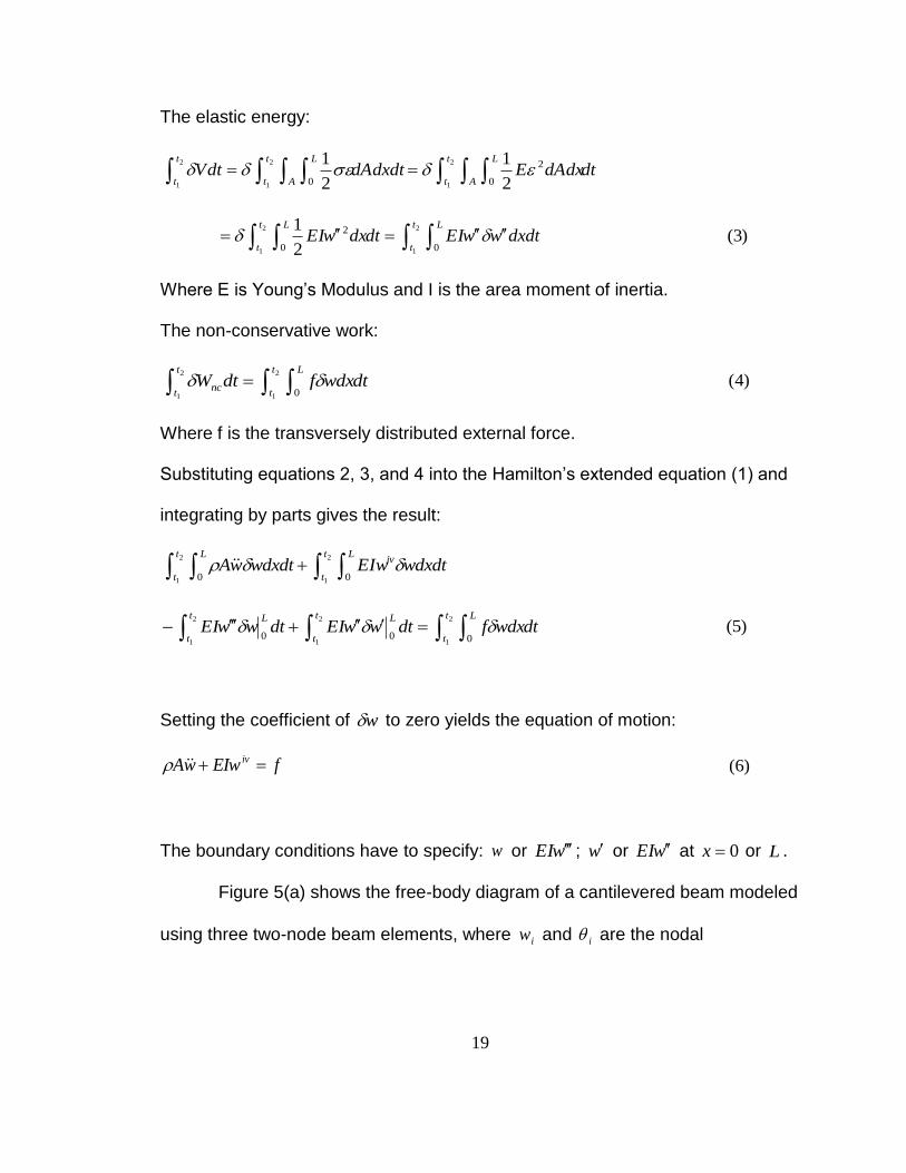
The elastic energy:
dtdAdxEdAdxdtdtVt
t A
Lt
t A
Lt
t 2
1
2
1
2
1 0
2
0 2
1
2
1
2
1
2
1 00
2
2
1 t
t
Lt
t
L
dxdtwwEIdtdxwEI )3(
Where E is Young’s Modulus and I is the area moment of inertia.
The non-conservative work:
2
1
2
1 0
t
t
Lt
tnc dtwdxfdtW )4(
Where f is the transversely distributed external force.
Substituting equations 2, 3, and 4 into the Hamilton’s extended equation (1) and
integrating by parts gives the result:
2
1
2
1 00
t
t
Liv
t
t
L
wdxdtEIwwdxdtwA
2
1
2
1
2
1 000
t
t
Lt
t
Lt
t
LdtwdxfdtwwEIdtwwEI )5(
Setting the coefficient of w to zero yields the equation of motion:
fEIwwA iv )6(
The boundary conditions have to specify: w or wEI ; w or wEI at 0x or L .
Figure 5(a) shows the free-body diagram of a cantilevered beam modeled
using three two-node beam elements, where iw and i are the nodal

20
displacements and slopes of each node, il is the elemental length of the ith
element, and )1(
1Q and )1(
2Q are the reaction force and moment acting on the first
node. As shown in Figure 5(b), each element has four unknown nodal
displacements. The displacement ),( txw within each element can be assumed
to be:
3
3
2
210),( xCxCxCCtx )7(
where x is a local coordinate with ilx 0 for the ith element.
Figure 5. (a) The free-body diagram; (b) the first element.
1w
1
)1(
1Q )1(
2Q
f
1l
2w
2 3w
3 4
4w
2l 3l
1w
1
2w 2
1l
(a)
(b)

21
For the first element:
01),0( Cwtw
11),0( Ctwx )8(
3
3
2
2102),( lClClCCwtlw
2
3212 32),( lClCCtlwx
Solving for iC in terms of iw and i , and then substituting the results into
equation (7) yields:
13
3
2
2
13
3
2
2
)2()231(),( l
x
l
x
l
xlw
l
x
l
xtxw
23
3
2
2
23
3
2
2
)()23( l
x
l
xlw
l
x
l
x )9(
Equation (9) can be rewritten as:
24231211 )()()()(),( xNwxNxNwxNtxw
}{}{}{}{ )1()1( wNNw TT , Twww 2211
)1( )10(
Where )4,3,2,1( iN i are known as the shape functions (Hermite cubic or spline
interpolation functions) given by:
3
3
2
2
1 231l
x
l
xN , )2(
3
3
2
2
2l
x
l
x
l
xlN
3
3
2
2
3 23l
x
l
xN , )(
3
3
2
2
4l
x
l
xlN )11(

22
It follows from equations (10) and (2) that:
dtdxwAwdxwAwdxwAwwdxdtwATdtt
t
l l lt
t
Lt
t
2
1
1 2 32
1
2
1 0 0 00
dtdxwNANwt
t
l TT
2
1
1
0
)1()1( )12(
2
1
2 3
0 0
)3()3()2()2(t
t
l l TTTTdtdxwNANwdxwNANw
dtwmwwmwwmwt
t
TTT
2
1
]][][][[ )3()3()3()2()2()2()1()1()1(
Where the elemental mass matrix is:
dxNANmTl
i i
0
)( ][ , 3,2,1i )13(
If and A are constants then:
22
22
)(
422313
221561354
313422
135422156
420
iiii
ii
iiii
ii
ii
llll
ll
llll
ll
Alm
)14(
The global (structural) mass matrix ][M can be obtained by assembling the
elemental mass matrices using the continuity of displacement and slope at each
node as:

23
)3(
44
)3(
43
)3(
42
)3(
41
)3(
34
)3(
33
)3(
32
)3(
31
)3(
24
)3(
23
)3(
22
)2(
44
)3(
21
)2(
43
)2(
42
)2(
41
)3(
14
)3(
13
)3(
12
)2(
34
)3(
11
)2(
33
)2(
32
)2(
31
)2(
24
)2(
23
)2(
22
)1(
44
)2(
21
)1(
43
)1(
42
)1(
41
)2(
14
)2(
13
)2(
12
)1(
34
)2(
11
)1(
33
)1(
32
)1(
31
)1(
24
)1(
23
)1(
22
)1(
21
)1(
14
)1(
13
)1(
12
)1(
11
0000
0000
00
00
00
00
0000
0000
][
mmmm
mmmm
mmmmmmmm
mmmmmmmm
mmmmmmmm
mmmmmmmm
mmmm
mmmm
M )15(
Similarly, it follows from equations (10) and (3) that:
2
1
2
1 0
t
t
Lt
tdxdtwwEIVdt )16(
dtdxwEIwdxwEIwdxwEIwt
t
l l l
2
1
1 2 3
0 0 0
dtdxwNEINwt
t
l T
xxxx
T
2
1
1
0
)1()1(
dtdxwNEINwdxwNEINwt
t
l T
xxxx
Tl T
xxxx
T
2
1
32
0
)3()3(
0
)2()2(
dtwkwwkwwkwt
t
TTT
2
1
]][][][[ )3()3()3()2()2()2()1()1()1(
Where the elemental stiffness matrix dxNEINkT
xx
l
xx
i i
0
)( ][ )3,2,1( i . If E
and I are constant, one can obtain:
22
22
3
)(
4626
612612
2646
612612
iiii
ii
iiii
ii
i
i
llll
ll
llll
ll
l
EIk )17(

24
The global stiffness matrix ][K is obtained by assembling the elemental stiffness
matrices as:
)3(
44
)3(
43
)3(
42
)3(
41
)3(
34
)3(
33
)3(
32
)3(
31
)3(
24
)3(
23
)3(
22
)2(
44
)3(
21
)2(
43
)2(
42
)2(
41
)3(
14
)3(
13
)3(
12
)2(
34
)3(
11
)2(
33
)2(
32
)2(
31
)2(
24
)2(
23
)2(
22
)1(
44
)2(
21
)1(
43
)1(
42
)1(
41
)2(
14
)2(
13
)2(
12
)1(
34
)2(
11
)1(
33
)1(
32
)1(
31
)1(
24
)1(
23
)1(
22
)1(
21
)1(
14
)1(
13
)1(
12
)1(
11
0000
0000
00
00
00
00
0000
0000
][
kkkk
kkkk
kkkkkkkk
kkkkkkkk
kkkkkkkk
kkkkkkkk
kkkk
kkkk
K )18(
The variation of non-conservative work, ncW , due to a distributed external force
f is given by:
dtwdxfwdxfwdxfdtwdxfdtWt
t
lllt
t
Lt
tnc
2
1
3212
1
2
1 0000
dtFwFwFwt
t
TTT
2
1
)3()3()2()2()1()1( )19(
where the elemental force vector due to the distributed load is ili dxNfF
0
)(. If
f is constant, )(iF for the ith element is given by:
T
iiiii flflflflF
122122
22
)( )20(
Then the global force vector due to the distributed load of this three-element
beam model is given by:
T
flflflflflflflflflflflflF
122121222121222122
2
33
2
3
2
232
2
2
2
121
2
11 )21(

25
The equation of motion for this finite element model is given
}{}{}]{[}]{[}]{[ QFwKwCwM )22(
where Q represents the global force vector due to concentrated loads on the
beam. For this three-element beam model:
TQQQ 000000)1(
2
)1(
1 )23(
and [C] is the damping matrix.
Assuming the system has no loads, external forces or damping the equation (22)
can be reduced to:
0}]{[}]{[ wKwM )24(
Assuming the displacement vector can be represented in the form:
tew }{}{ )25(
Then
tew }{}{ 2 )26(
where {} is the modal shape and is one of the natural frequencies.
Substituting (25) and (26) into equation (24) leads to:
}0{}]){[]([ 2 MK )27(
or in the generalized eigen-problem form:
}]{[}]{[ MK )28(
where the eigenvalues are the square of the resonate frequencies of the
structure and the eigenvetors {} are the modal displacements. Directly

26
following the references [57] and [65] the complete system of force displacement
equiations can be written, in matrix form, as:
0}{}{}]{[ QFwK )29(
This example was limited to 2 degrees of freedom per node to save space.
It is very easy to extend this example to more degrees of freedom. The FEA
developed for this research used 2 node beam elements with 6 degrees of
freedom per node. Also, the developed FEA code included the coordinate
transformations so that three dimensional structures could be analyzed. For a
complete treatment of the coordinate transformation see references [57, 65, 66,
and 67].
2.2 High-Speed FEA Approximation
Currently, the most common practice for finding the deflection, stress,
and/or natural frequency of a complex structure is to use FEA. When applied to
DSO problems some major problems arise. As a structure’s complexity
increases, the size of the global matrices in the FEA increases. As the numbers
of discrete members are added to the structure, the matrices become less sparse.
Also, since the design variable space is now discontinuous, derivative based
search algorithms have to search each and every discrete subspace. The large
non-sparse matrices increase the computation effort of the problem. One
solution is to approximate the FEA with some faster algorithm. The FEA has
multiple inputs such as node locations, material, and geometric properties of the

27
elements. The outputs are the nodal displacements and/or modal frequencies
(Eigenvalues). The relationship between the input and output is non-linear.
Currently, one of the most researched and effective methods of approximating a
non-linear system of multiple inputs and outputs, such as the structural analysis
problems with load as input and displacement or stress as output, is through the
use of an artificial neural network (ANN or NN) [68 and 69]. It is an obvious idea
to apply NN to FEA, however, very little research has been done [11 and 70].
The previous works suggested very different NN architectures. One suggested a
radial bias network [11], while the other had better results with a multi-layer feed
forward architecture [70]. This work [68 and 70] has shown a major decrease in
computational effort.
2.3 Basic NN Structure
The NN is simply a very large network of simple elements that are
modeled roughly after a living creature’s nervous system. One of the most
attractive aspects of a NN is the fact that the elements are arranged in a parallel
fashion. This leads to a parallel implementation in computer systems that in turn
lead to very fast computations. As in biological systems, the simplest elements
are called neurons.

28
Figure 6. A typical neuron
Figure 6 shows a typical neuron where the sum of the weighted input and bias
are transferred through the function f. The weight and bias become the design
variables that are adjusted so that the neuron can be trained.
Many transfer functions are available with the Matlab NN toolbox [69].
Three of the most commonly used functions are the sigmoid, hyperbolic tangent,
and linear functions. The following is a brief description of these functions.
Sigmoid function (LOGSIG):
nenf
1
1)( )30(

29
Hyperbolic tangent function (TANSIG):
11
2)(
2
nenf )31(
Linear function (PURELIN):
nnf )( )32(
Figure 7. Transfer functions

30
Figure 7 shows the transfer functions. The TANSIG and LOGSIG are the
so called “squashing” functions because they force the outputs to 0 to 1 or -1 to 1
respectively.
Figure 8. A typical 2 layer feed forward neural network
Figure 8 shows a typical network of neurons. Note how the structure is
inherently parallel in nature. Even though the neurons and structure are very
simple, if the numbers of neurons in the internal layers are large enough, the
network can be trained to represent complex non-linear systems. These large
NN’s are good at approximating practically any non-linear function [69]. The
number of inputs and outputs a NN can have is only limited by the computer

31
memory available. Therefore, a standard feed-forward NN of sufficient size
should be able to approximate most FEA models.
Normally the NN is trained to approximate a function so that a set of inputs
leads to a set of target outputs. In the case of approximating an FEA structural
model, the inputs would be the material and geometric properties (shape), node
locations, number and location of discreet components (topology), applied loads,
and boundary conditions. The outputs would be nodal displacements and/or
natural frequencies.
Figure 9. Neural network training flowchart

32
The training of a NN, as shown in Figure 9, is simply a large optimization problem
that uses the weight and bias as the design variables. Most practical NN
problems require many sets of inputs and targets to train. The literature
suggests an alternative to a feed-forward network [11 and 70]. A radial bias
network is the type that is very effective at non-linear approximations. They
generally require more neurons than a feed-forward network but train in much
less time [14].
Figure 10. Typical radial bias neuron
The typical radial bias neuron is shown in Figure 10. The distance between the
weight and input is multiplied by the bias and then sent to the radial bias function.
In practice the system will have multiple inputs so the distance between the
inputs and weights is their vector dot product. To train the radial bias network the
training routine will create as many neurons as there are inputs. The weights

33
and bias are then optimized. If the error goal is not met, more neurons are
added. Generally the number of neurons is much larger that the equivalent feed
forward network.
2.4 NN Test
The effectiveness of the use of NN’s as a FEA approximator was tested
using a simple cantilever beam. A prismatic beam 36” long with a height of 1”
and a width of 0.5” was selected. The beam was fixed on one end and a set of
forces were applied to the other (Figure 11).
Figure 11. Test cantilever beam
The set of forces were randomly selected in the range of 10lbs. to 250lbs. The
beam was discretized in to 10 equal elements with two nodes apiece for a total of
11 nodes. The displacements at each node were calculated using the elastic
equation:
PxEIy '' )33(

34
1"x0.5"x36" Simple Cantilever Beam with 90lbs load
Node Number 1 2 3 4 5 6 7 8 9 10 CPU Time
Exact -0.0041 -0.0157 -0.0340 -0.0582 -0.0875 -0.1209 -0.1577 -0.1971 -0.2381 -0.2799 0.0001
NN -0.0041 -0.0157 -0.0340 -0.0582 -0.0875 -0.1209 -0.1578 -0.1971 -0.2381 -0.2799 0.0042
FEA -0.0041 -0.0157 -0.0340 -0.0582 -0.0875 -0.1209 -0.1577 -0.1971 -0.2381 -0.2799 0.0470
Integrating equation (27) twice and appling the boundary conditions:
)23(6
323 LxLxEI
Py )34(
The displacements were also obtained using the FEA routine developed in the
previous section. The applied loads (inputs) and FEA results (outputs) were
used to train a standard feed-forward NN. The NN was then tested with an input
of 90lbs. Table 2 and Figure 11 show the results compared to the anaylitical and
FEA solutions. It also shows the average CPU times.
Table 2. Simple cantilever beam example displacements and CPU times

35
Figure 12. Simple beam nodal deflection.
The test was then repeated. This time the beam was changed to 1.75”
high by 0.25” wide. The previously “learned” weights and biases were used as a
starting point. The results are shown in Figure 13 and Table 3. Again, the FEA,
NN, and the analytical solutions are the same. However, there is a large
reduction in CPU time for the NN compared to the FEA. This reduction in CPU
time would justify the use of the NN but not on a simple FEA problem like this.
The NN training outweights any gains. However, retraining the already learned
network to a new but similar problem is very fast. Figure 14 shows the training
36
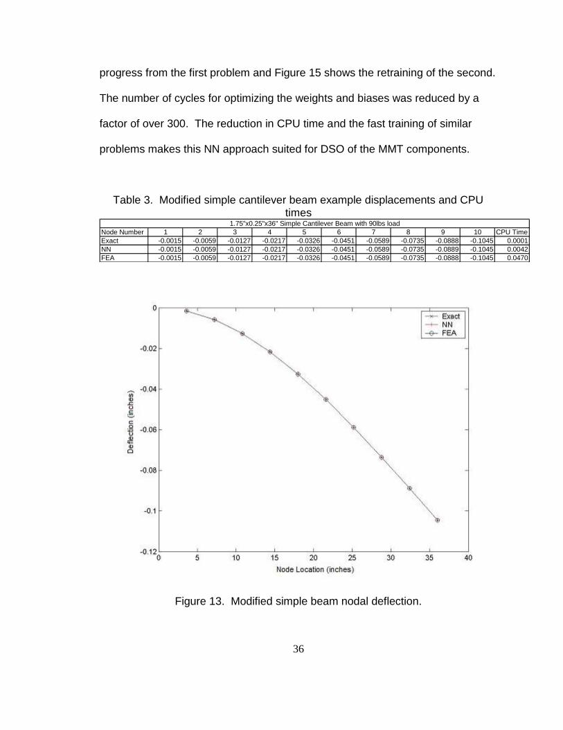
progress from the first problem and Figure 15 shows the retraining of the second.
The number of cycles for optimizing the weights and biases was reduced by a
factor of over 300. The reduction in CPU time and the fast training of similar
problems makes this NN approach suited for DSO of the MMT components.
Table 3. Modified simple cantilever beam example displacements and CPU times
1.75"x0.25"x36" Simple Cantilever Beam with 90lbs load
Node Number 1 2 3 4 5 6 7 8 9 10 CPU Time
Exact -0.0015 -0.0059 -0.0127 -0.0217 -0.0326 -0.0451 -0.0589 -0.0735 -0.0888 -0.1045 0.0001
NN -0.0015 -0.0059 -0.0127 -0.0217 -0.0326 -0.0451 -0.0589 -0.0735 -0.0889 -0.1045 0.0042
FEA -0.0015 -0.0059 -0.0127 -0.0217 -0.0326 -0.0451 -0.0589 -0.0735 -0.0888 -0.1045 0.0470
Figure 13. Modified simple beam nodal deflection.

37
Figure 14. NN training with no previous weights and biases.

38
Figure 15. Training using previous weights and biases.
To test the effectiveness of a feed forward NN an FEA model of the side of
a typical MMT base, shown in Figure 16, was created. The model was selected
as 12” high by 36” long and nonsymmetrical coupled loads of -100lbs and 700lbs
were applied. A training input set of 250 was created by randomly selecting the L
shaped cross sections (angle beam), in the range of 0.5 in2 to 2.0 in2, of the six
members. The target set of nodal deflections was then created by running FEA
on the 250 inputs. A feed forward NN was created and trained using the set of

39
random cross sections as inputs and the FEA nodal displacements as targets.
To validate the effectiveness of the NN, a set of four cross sections properties
were randomly selected from the available standard steel shapes. This set was
used to test the NN ability to approximate the FEA and to compare the CPU time
required for the calculations. These results are shown in Tables 4. Table 5
shows the standard steel element cross sections used for validating the NN.
Figure 16. Side view of a typical MMT base component

40
Table 4. Nodal displacement and CPU time
Table 5. Standard steel shapes
Test Number 1
node 1 2 3 4 5 6 7 CPU time
NN Displacements 0.0000 -0.0027 -0.0040 -0.0345 -0.0538 -0.0001 -0.0001 0.0075
FEA Displacements 0.0000 -0.0031 -0.0050 -0.0376 -0.0570 -0.0014 0.0000 0.0700
Difference 0.0000 0.0005 0.0010 0.0031 0.0032 0.0013 0.0001 0.0625
Test Number 2
node 1 2 3 4 5 6 7 CPU time
NN Displacements 0.0000 -0.0010 -0.0024 -0.0035 -0.0034 -0.0013 0.0000 0.0050
FEA Displacements 0.0000 -0.0014 -0.0028 -0.0040 -0.0039 -0.0016 0.0000 0.0603
Difference 0.0000 0.0003 0.0005 0.0005 0.0004 0.0003 0.0000 0.0553
Test Number 3
node 1 2 3 4 5 6 7 CPU time
NN Displacements 0.0000 -0.0012 -0.0031 -0.0059 -0.0065 -0.0015 0.0000 0.0050
FEA Displacements 0.0000 -0.0014 -0.0034 -0.0063 -0.0068 -0.0017 0.0001 0.0625
Difference 0.0000 0.0002 0.0003 0.0004 0.0004 0.0002 0.0000 0.0575
Test Number 4
node 1 2 3 4 5 6 7 CPU time
NN Displacements -0.0001 -0.0059 -0.0096 -0.0117 -0.0109 -0.0042 0.0000 0.0050
FEA Displacements -0.0002 -0.0059 -0.0095 -0.0118 -0.0110 -0.0040 0.0002 0.0600
Difference 0.0001 0.0000 0.0001 0.0001 0.0001 0.0002 0.0001 0.0550
Test Number Element 1 Element 2 Element 3 Element 4 Element 5 Element 6
1 L3/4x3/4x1/8 L2x2x1/2 L3/4x3/4x1/8 L1x1x1/4 L2x2x1/2 L2x2x1/2
2 L2x2x1/2 L2x2x1/2 L1x1x1/4 L1x1x1/4 L1x1x1/4 L1x1x1/4
3 L1x1x1/4 L2x2x1/2 L1x1x1/4 L1x1x1/4 L1x1x1/4 L1x1x1/4
4 L1x1x1/4 L1x1x1/4 L3/4x3/4x1/8 L3/4x3/4x1/8 L1x1x1/4 L1x1x1/4

41
Figure 17. Training time with no previous weights and biases
One interesting aspect of the NN is the ability to quickly learn new functions that
are close to the original. The topology in the previous model was slightly
modified as shone in Figure 18.

42
Figure 18. Modified structure topology
The same loads were applied and a new set of random training input data was
generated. New NN’s were created using the previous learned weights and
biases. These new NN’s were trained using the new topology and the maximum
deflections; the calculation times are shown in Table 6. The randomly selected
standard steel element cross sectional shapes are shown in Table 7.
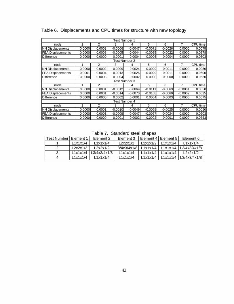
43
Table 6. Displacements and CPU times for structure with new topology
Table 7. Standard steel shapes Test Number Element 1 Element 2 Element 3 Element 4 Element 5 Element 6
1 L1x1x1/4 L1x1x1/4 L2x2x1/2 L2x2x1/2 L1x1x1/4 L1x1x1/4
2 L2x2x1/2 L2x2x1/2 L3/4x3/4x1/8 L1x1x1/4 L1x1x1/4 L3/4x3/4x1/8
3 L1x1x1/4 L3/4x3/4x1/8 L1x1x1/4 L1x1x1/4 L1x1x1/4 L2x2x1/2
4 L1x1x1/4 L1x1x1/4 L1x1x1/4 L1x1x1/4 L1x1x1/4 L3/4x3/4x1/8
Test Number 1
node 1 2 3 4 5 6 7 CPU time
NN Displacements 0.0000 0.0003 -0.0006 -0.0047 -0.0071 -0.0026 0.0000 0.0075
FEA Displacements 0.0000 0.0003 -0.0005 -0.0044 -0.0065 -0.0022 0.0000 0.0678
Difference 0.0000 0.0000 0.0001 0.0004 0.0006 0.0004 0.0000 0.0603
Test Number 2
node 1 2 3 4 5 6 7 CPU time
NN Displacements 0.0000 -0.0002 -0.0009 -0.0024 -0.0029 -0.0011 0.0000 0.0050
FEA Displacements 0.0001 -0.0004 -0.0013 -0.0026 -0.0029 -0.0011 0.0000 0.0600
Difference 0.0000 0.0003 0.0004 0.0002 0.0000 0.0000 0.0000 0.0550
Test Number 3
node 1 2 3 4 5 6 7 CPU time
NN Displacements 0.0000 0.0001 -0.0012 -0.0069 -0.0111 -0.0063 -0.0001 0.0050
FEA Displacements 0.0000 0.0001 -0.0014 -0.0070 -0.0108 -0.0060 -0.0002 0.0625
Difference 0.0000 0.0000 0.0002 0.0001 0.0004 0.0003 0.0000 0.0575
Test Number 4
node 1 2 3 4 5 6 7 CPU time
NN Displacements 0.0000 0.0001 -0.0010 -0.0049 -0.0069 -0.0025 0.0000 0.0050
FEA Displacements 0.0000 0.0001 -0.0009 -0.0047 -0.0067 -0.0024 0.0000 0.0603
Difference 0.0000 0.0000 0.0001 0.0002 0.0002 0.0001 0.0000 0.0553

44
Figure 19. Time to retrain NN
A couple of interesting observations can be made from these results. First,
the feed-forward NN was effective at approximating the FEA. The largest
displacement error in this test was 0.001 inches and most of the errors were less
than 0.0005 inches. This is much less than the displacement constraint used
when the optimization of the MMT components. Second, the NN had order of
magnitude reductions in computation times. The radial bias method failed to
converge with this problem. The feed forward NN had better results and faster
training times. Also, with the feed forward NN major reductions in training times
can be realized by using information from previous networks.

45
2.5 NN training
Many methods to train NN’s are included in the Matlab NN toolbox. Some
of these algorithms are not useful for practical problems and the best method for
fastest training is dependent on the problem [69]. The best training algorithm for
a given problem depends on many factors, such as the size of the training set,
the complexity of the problem, the size of the network, and the type of the
problem (pattern recognition of function approximation) [69]. The easiest and
fastest way to determine the best and fastest converging algorithm is by trial-and-
error. Four of the most common high-performance algorithms were tested.
The four algorithms tested were the Matlab functions traingda, trainrp,
trainscg, and trainlm. The first method was the steepest gradient descent with a
variable step size (TRAINGDA). The second was the resilient back-propagation
(TRAINRP) method. All of the networks in this research were used to
approximate non-linear systems. This requires the use of “squashing” functions.
Squashing functions take an infinite input and output with a range of -1 to 1. As
the input gets very large or very small, their derivative goes to zero. This has a
major impact on the steepest descent gradient based methods. The gradient
may be very small while the network is training. This in turn causes very small
changes in the weights and biases even though they are far from converging.
The trainrp uses only the sign of the gradient, not the magnitude. It uses a
separate variable for the step magnitude. This variable increases if the sign of

46
the gradient stays the same from step to step or decreases if the sign changes.
This leads to faster learning and tends to reduce oscillations around the solution.
The third algorithm tested performs a search along the conjugate gradient
instead of the steepest descent direction (TRAINSCG). This usually produces
faster convergence. The last algorithm tested used a modified Newton method
(TRAINLM) that has a variable step size and direction. The TRAINLM function
generally has the ability to train to a lower error level.
Figures 20, 21, 22, and 23 show the progress of training the networks
derived from the structure shown in Figure 16 using the different algorithms. For
the networks in this research the TRAINRP seemed to have the best
performance when the error was higher. The TRAINLM had the best
performance when training to a lower error. In all the proceeding tests and
programs the TRAINRP was used for initial training then TRAINLM was used to
reach a lower error.

47
Figure 20. Training history for traingda

48
Figure 21. Training history for trainrp

49
Figure 22. Training history for trainscg

50
Figure 23. Training history for trainlm

51
2.6 General comments and results from NN test
The NN is not a cure all for computationally inefficient problems. It is,
however, proven very useful in optimal MMT design. The following are some
brief comments on NN.
The steps to create and use a NN:
1. Develop the network structure. This must be large enough and have
enough hidden layers to represent the problem. There is no theoretical
method to determine the correct structure. It is generally done through
trial and error.
2. Train the network. This is a large scale optimization problem.
Accepted optimization techniques can be applied.
3. Simulate the network. New inputs are given to the network. What was
learned in the training is recalled and new outputs are produced.
NN structures are inherently parallel. This leads to easy implementation
to parallel computers and processors which leads to fast computations.
However, this research was developed on a single computer and
processor.
Training is just a large scale optimization process. The weights and
biases of the NN are adjusted (design variables) thereby minimizing the
error between a known target and the output of the NN.

52
The NN method can be a very effective universal approximation for FEA.
However, the structure and the transfer functions must be carefully chosen.
The number of nodes must be sufficiently large and the use of some non-
linear transfer functions is required.
For this research feed-forward NN gave better results than the radial bias
networks.
NN based FEA approximations are better at interpolation than
extrapolation.
NN calculations are much faster than FEA calculations. Generally, they
are at least an order of magnitude faster. As the size of the of the problem
increases, the NN calculations increase linearly while the FEA calculations
increase exponentially.
Even though the use of NN approximation of FEA leads to faster calculations,
FEA calculations should not simply be replaced with NN. The real advantage is
to use the inherent “memory” properties of the NN along with the computational
efficiencies to utilize previous designs. In other words, as new components are
developed the optimal designs are captured in the NN and will influence future
designs.
2.7 Optimization Algorithms
In this study the stated problem of optimizing MMT structures is
completely discrete in nature. According to the literature review, most of the

53
previous work focused on GA, SA, or branch and bound methods for completely
discrete problems. Also, guaranteeing that the GA or SA produced a global
optimum is difficult. No clear mathematical proof exists to prove a global
optimum is achieved. Branch and bound, on the other hand, is a global
optimization algorithm. It may not be the most efficient, but at least it operates in
polynomial time on general problems.
For this research a branch and bound method was used as the primary
optimization algorithm. The branch and bound method has some other added
properties that help meet the objectives of this project. It was shown previously
that for practical real-world problems the FEA models would get large and an
approximation is needed. The problem is when to use the FEA and when to
switch to the approximation method? The branch and bound method has a clear
point to make the switch. When the variables are relaxed the FEA is used and a
neural network training set is generated. When the branches are fathomed with
discrete variables the approximation is used. This has the advantage that most
of the design space will be covered when the FEA is used and the training set is
developed. A very robust NN approximator is developed using this method
because the NN is generally better at interpolation than at extrapolation.
Applying the branch and bound method to the MMT optimization problem
is not without challenges. Typically, the branch and bound method is used with a
linear programming or gradient descent for the relaxation method [13]. However,
these methods are not effective on non-convex or discontinuous problems [13].

54
The discrete MMT problem is both non-convex and discontinuous. For this study
a robust continuous optimization algorithm is required for the relaxation.
Generally, the literature suggests a GA or SA based algorithm to overcome these
problems [4 and 13]. However the literature also suggest these algorithms may
be difficult to tune and implement. In recent years many researchers have
successfully applied PSO to these types of discontinuous problems. The PSO
has the advantages of being simple and easy to implement. It has also been
shown to converge rapidly but it is difficult to specify the stopping criteria. For
this reason a hybrid approach was chosen by using a PSO to quickly converge
toward the best solution then switch to a fast gradient based method to converge
on the solution. This PSO method had the added benefit of finding solutions
distributed over the entire design space. This generally improved the training
performance of the neural network.
2.8 Branch and Bound Discrete Optimization
A review of the current literature revealed that exhaustive enumeration is
only possible for trivial problems [4 and 13]. Partial enumeration or heuristic
methods are required for practical problems. One problem with heuristic
methods is that it is very difficult to prove they will produce a global optimum on
practical problems. The partial enumeration methods, specifically the branch and
bound, method over-comes these problems [71]. It will produce a global
optimum and in most cases it will operate in polynomial time.

55
The branch and bound method is based on the fact that the relaxed
continuous solution is always better than the discrete solution. Using this fact,
bounds can be created and large groups of potential discrete solution can be
eliminated. The algorithm creates a tree structure with branches by
systematically fixing and relaxing discrete variables. This creates a structure with
nodes connected by links. Following the best path through the links and nodes is
called fathoming. The use of the branch and bound method is best described
with an example.
Consider the structural bracket shown in Figure 24. Assume the goal is to
minimize the total amount of material in the structure and elements 1 and 2 can
only be made of standard steel round bar stock. Also, assume the end of
element 2 can assume only the two locations shown in the figure. The questions
are: What is the optimal layout of element 2? What are the optimal cross
sections of both elements? The bracket must not deflect more than 0.010” when
it is supporting 30lbs.
Figure 24. Structural Bracket Example

56
The formal optimization problem can then be stated as:
Minimize: 232
1
22321 )
2)()(144()
2(24),,(
xx
xxxxf
]24,12[1 x
]25.1,0.1,5.0[2 x
]25.1,75.0,125.0[3 x
Subject to: 010.0
Where: is the maximum nodal deflection
X2 is the diameter of element 1 cross section
X3 is the diameter of element 2 cross section
The first variable x1 is fixed and partial solutions are found. In this case x1
only has two discrete possibilities. So, x1 is fixed to these two values and the
other variables are relaxed. In this example, a sequential quadratic programming
method was used to find the optimal solutions. As shown in Figure 25, this
produces two branches or partial solutions from node 0.
This method of fixing and relaxing variables is continued by following the
path of the best solution until the tree is completely fathomed. Then, the partial
solutions that are worse than the best fathomed solution are pruned or cut. This
will leave only active or pruned partial solutions. An active partial solution is one
that is not pruned but has not been fathomed. This is continued until all
branches have been fathomed or pruned.

57
Figure 25. Branch and Bound Tree for the Structural Bracket Example
Structural Bracket Example
Start Node 0:
Root node where all variables are relaxed.
Node 1 & 2:
Discrete variable x1 is assigned to each permissible discrete value. This
creates two paths or branches. The optimal solution is found for each
node by relaxing the other variables. Node 1 has the best solution so it
will be fathomed.
Completion of Node 1:

58
Node 1 is expanded by setting the discrete variable x2 to its permissible
discrete values. This creates branches to nodes 3, 4, and 5. Node 3 has
the best solution so it will be fathomed.
Completion of Node 3:
Node 3 is expanded by setting the discrete variable x3 to its permissible
discrete values. This creates branches to nodes 6, 7, and 8. Node 6 fails
to produce a solution because it does not meet the displacement
constraint. Node 7 produces the best solution. Since all the discrete
variables at node 7 are assigned discrete values the solution at node 7 is
considered the current best discrete solution. All of the nodes with
solutions greater than node 7 are pruned.
All of the nodes have been pruned or fathomed. Therefor, node 7 is the global
discrete optimal solution.
This example shows that the branch and bound method is effective in
finding the global optimum of a typical discrete structural optimization problem.
In this example a non-linear relaxation method was applied. Also, the algorithm
used the non-equality constraint as an effective pruning mechanism.
The MMT optimization problems of this study were solved using the
branch and bound method by fixing one variable at a time then relaxing the other
variables. Fixing one variable at a time broke the problem into branches. These
branches were then solved as continuous optimization problems. The
continuous branches were then compared to discrete solutions and were

59
normally cut after a few iterations. This method was based on the fact that the
continuous solution of each branch was always more optimal than the discrete
solution. Also, the use of gradient-based methods provided continuous solutions
with very little computational load.
For the MMT DSO problems branches were the topology of the structure.
Another discrete design variable is the different shape of cross-sections of each
structural members. The member’s geometric properties were then relaxed and
the continuous problem was solved. Figure 26 of the 2D problem of a typical
side of a MMT base shows the typical branches. Figure 27 shows the overall
flow of the branch and bound program as applied to the MMT DSO.

60
Figure 26. Tree for typical MMT base side
Figure 27. Branch and bound flowchart for MMT base side

61
For this research all of the members were assumed to have stock equal or
unequal leg L cross-sections. This assumption leads to three design variables
for each member (L1, L2, and t in Figure 28). Figure 28 also shows a typical
branch topology; in this example there are 6 elements with 3 design variables or
18 continuous variables for this branch.
Figure 28. Typical topology and cross section
It was determined from testing examples that many of relaxed continuous
optimization problems in this branch and bound structure were non-convex,
discontinuous, or had many local minimums. Many of these branches had long
convergent times when the variables were relaxed. It was obvious that some
non-gradient methods were needed.
2.9 Hybrid continuous optimization Conventional gradient-based optimization methods are very fast in solving
smooth convex problems. However, for piecewise continuous, non-differentiable,
or problems with many local minimums, they may become inefficient. In these

62
problems it was easy to see that each element was continuous but when
assembled, it became piecewise continuous with many local minimums.
The most effective way to solve this type of non-smooth problem was to
use a non-gradient based method. The most accepted non-gradient based
methods include SA, GA, and pattern search algorithms [4 and 72]. These
methods all have the problem that though they are assumed to be global
algorithms, they may be slow to reach the required accuracy and global optimal.
One method reported to overcome this problem was to employ a hybrid
approach that used both gradient and non-gradient based methods [72]. For
problems like this with many smooth areas or local minimums, a SA, GA, or
pattern search method was used to quickly get to the best smooth area then a
fast gradient based method was used to find the accurate solution.
SA, GA, and pattern search methods can be difficult to implement and
tune for a given problem [72]. Particle swarm optimization (PSO) is one of the
methods to overcome parameter tuning difficulty. It is loosely based on animal
swarming behavior by bees, birds, or fish. Compared to the other methods, it is
easy to implement and has few parameters to tune [73].
PSO simulates the behaviors of feeding schools of fish or flocks of birds.
The idea is simple. The swarm randomly heads out into a search area. The
swarm then moves in the general direction toward the individual with the most
food (best solution). The swarm moves together in general but individuals still

63
have some small random area to explore. After a very short time the swarm will
converge in the area with the most food (best solution).
The algorithm for a PSO is not difficult to develop, implement, and tune
[34]. First, the PSO is initialized with a group particle. The size of the swarm is
the first parameter. Normally this is set to 25 to 50 particles [73]. This is arbitrary
and dependent on the size of the search space. Second, the particles are
randomly distributed across the design space and the solution (fitness) for each
particle is found. The two best fitness values are stored. One is the value of the
best particle called “pbest”; the other is what will become the overall or global
best called “gbest”. After “pbest” and “gbest” are found, a velocity is found that
will move all the particles in the general direction of the best solution.
[])[](*()*1[][] locationpbestrandcVV
[])[](*()*2 locationgbestrandc )35(
where:
rand() is a vector of random numbers from 0 to 1
c1 and c2 are learning factors normally set to 2
location[ ] is the location of the particles in the design space
Location is a commonly used term in the PSO literature. It refers to the
current values of the design variables in the design domain [31]. Then, for every
iteration the location of the particles are updated:
[][][] Vlocationlocation )36(

64
The new velocity and locations are computed for each iteration. The
algorithm is continued until the maximum number of iterations is reached or the
change in “pbest” reaches a set minimum.
Compared to other optimization methods, the PSO tends to converge
quickly on the solution but may take many iterations to reach a desired minimum
error [73]. For this research a PSO with 50 particles was used and after 4
iterations it was assumed to be close to the global solution. The results of the
PSO were then used as the initial values for the standard Matlab gradient based
constrained nonlinear optimization function. The Matlab function quickly
convereged on a feasible solution. In this research the Matlab fmincon function
using the sequential quadratic programming algorithm option was used
exclusively. Figure 28 shows the flow diagram for the algorithm used to optimize
each branch of the problem. The current literature suggest there is no
mathematical proof to show the swarm has found a global solution. However, it
suggests that a large swarm (greater than 20 particles) will find the area of the
global solution, for most problems, in very few iterations [31].

65
Figure 29. Particle swarm optimizer flowchart

66
CHAPTER 3
DISCREET OPTIMIZATION OF MMT STRUCTURES
3.1 Application of DSO, FEA, and NN
The side of a typical MMT base component was selected to test the
combination of DSO using a branch and bound algorithm while using a parallel
training NN method. A structure like the one in Figure 16 was developed. A fully
grounded structure was considered. Throughout the design process elements
were added and removed and the cross section of the elements were changed.
This created a discrete topology and size problem. It was a discrete topology
problem because the elements could be located at any of the discrete node
locations. Also, removing or adding the elements was considered. The discrete
sizing was used because the material properties and cross sections of all the
elements were selected from the standard steel cross sections in Table 1. The
formal optimization problem can be stated as:
Minimize:
eN
i
iii LAW1
)37(
Subject to:
Displacement
01m ax
ik 3,2,1;,1 kNNi )38(
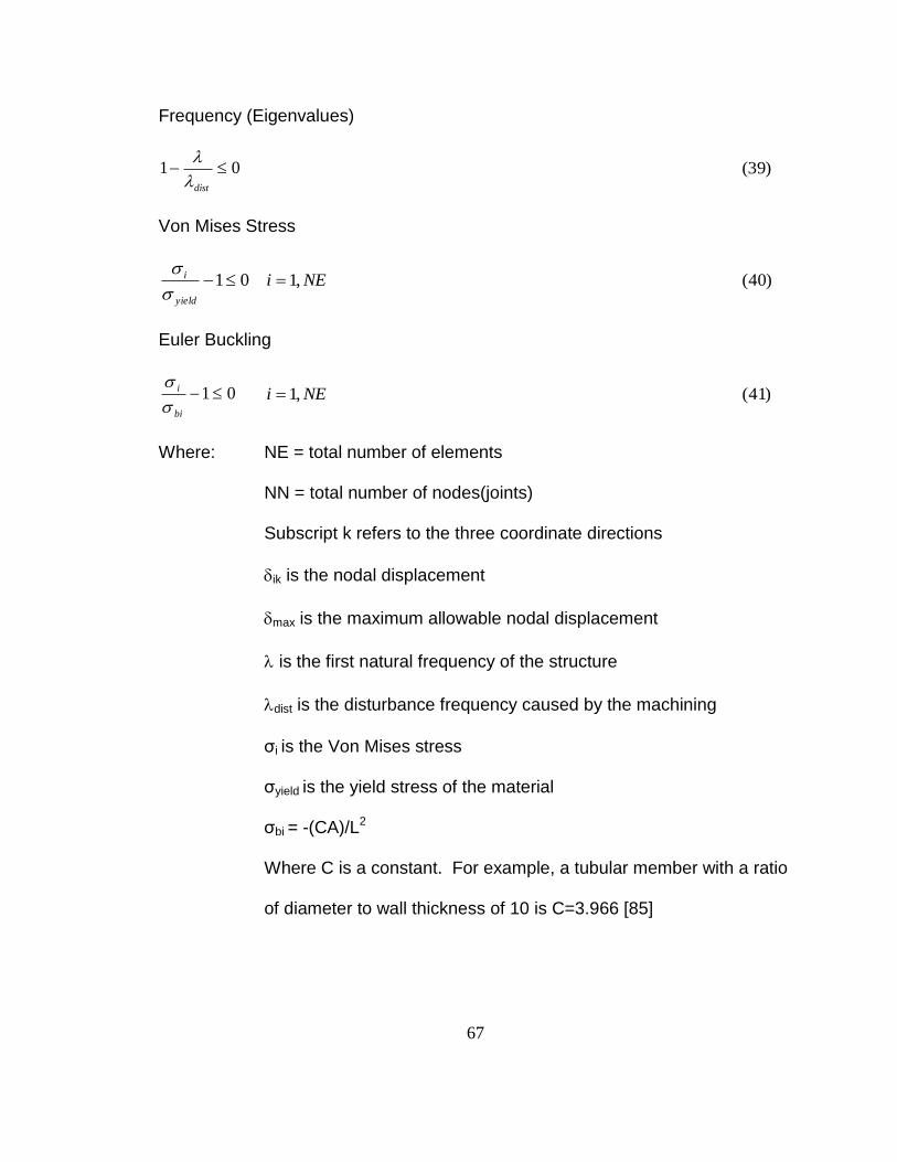
67
Frequency (Eigenvalues)
01 dist
)39(
Von Mises Stress
01yield
i
NEi ,1 )40(
Euler Buckling
01 bi
i
NEi ,1 )41(
Where: NE = total number of elements
NN = total number of nodes(joints)
Subscript k refers to the three coordinate directions
ik is the nodal displacement
max is the maximum allowable nodal displacement
is the first natural frequency of the structure
dist is the disturbance frequency caused by the machining
σi is the Von Mises stress
σyield is the yield stress of the material
σbi = -(CA)/L2
Where C is a constant. For example, a tubular member with a ratio
of diameter to wall thickness of 10 is C=3.966 [85]

68
For typical machine tool design the displacement (rigidity) constraint is very small
and therefore critical. The stress and buckling are far from critical so they can be
removed from the optimization problem. For this MMT model, only the
displacement and eigenvalues were considered for constraints.
Using only two internal elements and limiting the elements to four
standard cross sections produces over 450 thousand discrete combinations.
Using full enumeration and testing, each combination with FEA would require
approximately five days of computational time. These computing time
calculations are based on CPU times from a computer with a 2.33GHz Intel Core
2 Duo processor and 1Gbyte of RAM. Although this is not completely impractical,
if just a few more members or cross sections are considered the problem
becomes impractical and the idea of optimizing a complete MMT component is
unobtainable. However, if NN approximation and branch and bound techniques
are applied even complete MMT components can become practical. Figure 30
shows the general flow chart for the program. This research used only an
interpretive computer language (Matlab). Considerably faster computing times
could be realized using a compiler language such as FORTRAN or C thus
leading too larger scale problems. It is assumed that similar reductions in CPU
times would be realized using the methods developed in this research when
implemented with compiled code.

69
Figure 30. Parallel NN training and branch and bound
A program was developed to test this method on a side of a simple MMT
base component like the one shown in Figure 16. Subprograms for the FEA and

70
NN were developed using Matlab. Even though only one computer was used in
these tests the subprograms were used in a parallel method as shown in the flow
diagram. These could easily be implemented on separate processors for large
scale problems. The method was compared to the standard branch and bound
method using only FEA.
Table 8. Optimization results for first load condition
Figure 31. Optimal topology with element numbers for first load condition
Table 8 and Figure 31 show the results of both methods. Both methods have the
same topography and material cross sections. However, the NN approach used
Total CPU Volume
Member 1 2 3 4 5 Time (s) in^3
FEA L3/4x3/4x1/8 L2x2x1/2 L3/4x3/4x1/8 L3/4x3/4x1/8 L1x1x1/4 14.415 45.5156
NN L3/4x3/4x1/8 L2x2x1/2 L3/4x3/4x1/8 L3/4x3/4x1/8 L1x1x1/4 1.162 45.5156

71
much less CPU time. This is a significant reduction in time and this reduction
should get larger as the problem gets larger. The reduction in time will increase
for two reasons. First, the FEA computations will be longer. Second, since the
NN is trained for all the topologies, the time to remesh the FEA will be eliminated.
The test was then repeated with the loads applied in different locations to
simulate the MMT doing some common type of machining operation. Figure 32,
33, and 34 show the resulting optimal configurations. Table 9, 10, and 11 list the
results.
Figure 32. Optimal design for second load location

72
Table 9. Optimization results for second load condition
Figure 33. Optimal design for third load location
Table 10. Optimization results for third load condition
Total CPU Volume
Member 1 2 3 4 5 Time (s) in^3
FEA L1x1x1/4 L2x2x1/2 L3/4x3/4x1/8 L2x2x1/2 L1x1x1/4 58.773 92.6745
NN L1x1x1/4 L3/4x3/4x1/8 L1x1x1/4 L1x1x1/4 L3/4x3/4x1/8 4.618 75.5262
Total CPU Volume
Member 1 2 3 4 5 Time (s) in^3
FEA L1x1x1/4 L2x2x1/2 L3/4x3/4x1/8 L3/4x3/4x1/8 L3/4x3/4x1/8 30.04 61.5469
NN L1x1x1/4 L2x2x1/2 L3/4x3/4x1/8 L3/4x3/4x1/8 L3/4x3/4x1/8 2.444 61.5469

73
Figure 34. Optimal design for fourth load location
Table 11. Optimization results for forth load condition
Total CPU Volume
Member 1 2 3 4 5 Time (s) in^3
FEA L1x1x1/4 L1x1x1/4 L3/4x3/4x1/8 L3/4x3/4x1/8 L3/4x3/4x1/8 14.23 50.625
NN L1x1x1/4 L1x1x1/4 L3/4x3/4x1/8 L3/4x3/4x1/8 L3/4x3/4x1/8 1.202 50.625

74
3.2 Traditional Topology Optimization
The more traditional methods of topology optimization are well researched
and many examples of programming code can be found in the literature [75].
Examples of running code can even be found on the internet [74]. Designs can
be submitted and the topology takes shape real-time. Using this online code the
typical MMT base-side developed previously was tested.
Figure 35. Optimal topology using material density method
Figure 35 shows some typical results from these tests. When compared to the
branch and bound method used previously very different results were obtained.
This is because the online program is very limited in the number and types of
forces and boundary conditions that could be applied.
Several commercial software packages exist for solving topology
optimization problems. These programs are closely tied to commercial FEA
packages and have the same drawbacks as the commercial FEA packages. For

75
this research a very robust simple topology optimization routine was utilized.
This was done by adding to and modifying Matlab code that was developed by
others for public research and education projects [75]. The developers of this
code included a simple but effective FEA routine that is built into the topology
optimization code. The code was modified to accept the initial and boundary
conditions and the applied loads for the two-diminsional MMT base side.
This code was based on the solid isotropic material with penalization
(SIMP) approach [76]. In this approach the objective is to minimize the
compliance of the system. The formal optimization problem can be stated as:
Minimize:
KUUxc T)( )42(
or in terms of the elements:
N
e
ee
T
e
p
e ukuxxc1
)()( )43(
Subject to:
fV
xV
o
)(
FKU
10 x To avoid singularity x is greater than and not equal to 0.
Where:
euandU are the global and elemental displacements
F is the global force vector

76
ekandK are the global and elemental stiffness matrices
x is the design variable (relative density)
N is the design domain
p is the penalization constant
)(xV is the material volume
oV is the design domain volume
f is the prescribed volume fraction
The FEA for this problem was discretized into square elements with nodes
at each corner. The nodes had 2 degrees of freedom. The elemental stiffness
matrix was derived using the method previously described.
The optimization part of the code used a heuristic updating method that
directly follows the literature [56, 75 and 77]. The design variables were
formulated as:
n
eee
e
e
n
ee
m
e
n
ee
e
n
ee
e
new
e
Bxmxif
mx
mxBxxxif
Bx
mxxBxif
mxx
x
),1min(
),1min(
),,1min(),max(
),,max(
),max(
min
min
min
)44(
Where:
m is the move limit
n is the damping coefficient and is set to 0.5

77
eB is the optimality condition
e
e
e
x
V
x
c
B
)45(
Where:
is the Lagrangian multiplier
ex
c
is the sensitivity of the objective function, and
ee
T
e
p
e
e
ukuxpx
c 1)(
)46(
One major problem existed with implementing this approach. The
existence of a solution was not ensured and the results were sensitive to how
refined the domain was discreetized. Spatial zones of oscillation occured
frequently. This is commonly called the checker-boarding phenomenon [56, 77,
78, and 79]. A filter method that was adapted from digital image processing was
shown to reduce or eliminate these problems [75]. Directly following the
literature the mesh-independent filter is [74 and 75]:
N
f f
ffN
f
fee x
cxH
Hx
N
x
c
1
1
ˆ
ˆ
1
)47(
Where:
NerfedistNffedistrH f ,,1,),(|),,( minmin

78
The new mesh-independent filtered sensitivities (47) are used in place of the
original sensitivities (46).
This code was tested on the typical MMT base-side. Figure 36 shows the
results with the same loads and boundary conditions from the previous test
applied.
Figure 36.(a) Load Case 1
Figure 36.(b) Load Case 2

79
Figure 36.(c) Load Case 3
Figure 36.(d) Load Case 4
Figure 36. Optimal topology using material distrubution method
These results show very different topologies than the ones from the
branch and bound method. There are several reasons for the differences. First,
the branch and bound method used a constrained optimization method with very
small constraints on the displacement (x, y and rotation around z for the nodes
along the top edge of the structure) and natural frequency and the material
volume was minimized. The material distribution method minimized the
compliance of the structure and the material volume was an equality constraint.

80
Sankaranarayanan et al. compared topology optimization of trusses for minimum
weight using a method with stress and displacement constraints to a method
using a minimum compliance constraint. They showed for some truss problems
the stress and displacement constraint method produced different and generally
better results [84]. Second, the branch and bound includes the inherent
constraints that the members must be terminated at discrete nodes. Finally, the
literature suggests the material distribution method may not be the most effective
for layout problems like this if the prescribed fraction of material volume is too low
compared to the design domain volume [75 and 76]. For this code and this
problem, it was found that it failed to converge with prescribed volumes less than
approximately 25 percent. It was also found through experimentation that the
online code failed to converge with prescribed volumes less than approximately
25 percent. However, feasible optimal designs were found that had less than 10
percent of the actual design domain using the branch and bound method. Some
topologies were found to have less than 4 percent. Actually, for most structural
steel designs, using standard shapes and minimizing the amount of steel used,
this material distribution method may not be effective because the space frame
or truss would generally include less than 25 percent of the total volume. This
method would be better suited for plastic molded, cast metal, or formed sheet
metal designs where the material volume is a greater percent of the total design
space and rib or reinforcing member location would be total a continuous varible.

81
The test was repeated. This time a lateral force was add along with the
vertical force to simulate a typical milling operation. The results from the branch
and bound method using NN is shown in figure 37. Figure 38 through 41 show
the results from the material density method with varying amounts of percent
material. As expected with lower amounts of material (25% to 30%) the method
tends to converge slowly on a solution. With larger amounts of material the
results are close to the branch and bound method and the topologies are similar.
Figure 37. Discrete optimization using NN with lateral load

82
Figure 38. Discrete optimization using the material density method and 25% volume
Figure 39. Discrete optimization using the material density method and 30% volume
Figure 40. Discrete optimization using the material density method and 40% volume

83
Figure 41. Discrete optimization using the material density method and 50% volume
3.3 Large Scale MMT Base Optimization
The use of the branch and bound DSO routine was tested on a typical
MMT base. This included using a hybrid continous optimization approach for
each branch. This combined a traditional gradient based method with the PSO
method. The inputs and results from each branch or topology were saved and
later used for the NN training. After the initial NN was trained for the first
topology the weights and biases were saved for future training. Nonsymmetrical
multiple loads were applied to simulate a typical machining operation. A
common MMT base size of 36”x12”x12” was selected. A set of 3 standard L
channel steel shapes that ranged in flange size from ¾” to 2” and in flange
thickness from 1/8” to ½” were selected as the discrete set. Table 12 shows the
DSO results along with the CPU times.

84
Table 12. Element sections and CPU times for 3D MMT base
Element Standard
Number Steel L Shape
1 L3/4x3/4x1/8
2 L2x2x1/2
3 L3/4x3/4x1/8
4 L2x2x1/2
5 L2x2x1/2
6 L3/4x3/4x1/8
7 L2x2x1/2
8 L3/4x3/4x1/8
9 L2x2x1/2
10 L1x1x1/4
11 L1x1x1/4
12 L2x2x1/2
13 L1x1x1/4
14 L2x2x1/2
CPU Time 6h 19min.
One result that should be noted from this test is that the NN training for
this large scale problem was approxiamately 5 minutes. This is insignificant
compared to the over 6 hours it took to solve this 3 dimensional large-scale
problem. Given the number of function calls required to solve this problem using
the NN approach and the average time for the FEA of this structure, the problem
would take approximately 150 hours to solve just using FEA. This is not
imposible, but it is impractical and was not completed for this case. The code for
this project was developed entirely on an interpretative based computer language.
If it was developed or converted to a compiled language such as FORTRAN
much lower CPU times could be realized. However, the relative reduction in
times is a good indication of how effective this approach is on practical industrial
problems. The final optimal topology with the applied loads is shown in Figure 42.
To help visualize the results and topology a Matlab function was developed that

85
created an AutoLISP program. This AutoLISP program was then run in AutoCAD
to produce a detail 3D drawing of the final design (Figure 43). This is useful in
not only seeing the topology but the orientation of the cross sections of the steel
shapes.
Figure 42. The optimal topology with applied loads
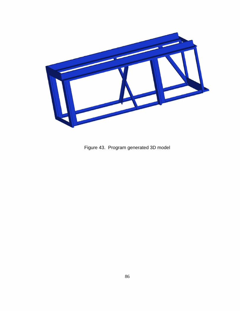
86
Figure 43. Program generated 3D model

87
CHAPTER 4
CONCLUSTION AND FUTURE WORK
4.1 Conclusion
A unique and novel method of discrete optimization has been developed
for the design of MMT components. A branch and bound method was used that
included a method that was parallel in nature to generate the data needed to
train a feed-forward NN. The continous optimization of the individual branches
used a hybrid method that combined particle swarm and traditional gradient base
optimization. This hybrid method proved effective in optimizing the piecewise
continous branches while at the same time generating data that became useful
for training the NN. The feed-forward NN was then shown to be effective at not
only approximating the FEA but also the inherent memory of the network became
useful for approximating similar disigns. The method was tested on a large scale
3D problem and it was shown that using only the FEA the problem becomes
impractical but implementing the NN along with the FEA makes it feasible. The
overall results from this research can be summarized as follows:
The use of a feed-forward NN was very effective as a FEA approximator.
The NN was effective at approximating more than just the FEA, for
example, multiple meshings of the FEA, multiple topologies, and
eigenfrequencies.

88
The hybrid approach was required for the continouis part of the branch
and bound method because of all the local minimums. This also helped
generate the training data for the NN.
The traditional material distribution methods of topological optimization are
not suited to this type of discrete structural optimization problem because
the amount of material volume compared to the total design space volume
is very small.
The method was successful on a large-scale structure that would be
impractical using other methods.
4.2 Future Research
In this problem the FEA was limited to linear elastic members. This
method of using NN approximation should be very effective on non-linear
elements. Fluid mechanics, heat transfer, and impact problems are just a few of
the FEA problems that when applied to large-scale optimization problems are
computationally expensive. The NN’s in these cases could be taught whole
families of similar problems with many of the pre and post processing operations
included in the NN.
All of the joints in this research were considered to be fixed and solid.
Refering to Figure 42 it can be seen that some of the joints would be impossible
to connect. This is because the optimization routine considered the orientation of
the cross sections. Also, a completely fixed solid joint is not practical. A

89
complete study of the joints should be considered. A method of quickly building
and recycling of MMT components will require a complete and detail design of
the joints.
The NN structure is very significant in the success of the structure
optimization. In this study, large NN structures were used. This structure was
large enough to handle any of the topologies and parameters. However, the
structure was almost always larger than required. Further studies should include
an adaptive type of NN structure.
The whole branch and bound process and the NN method is inherently
parallel. It would take very little effort to convert the code used in this research to
run over a network on multiple computers. Each continous branch or topology
could be optimized on a separate computer. Then, as each branch finished each
computer could start training individual NN’s. The NN’s could then easily be
implemented on multiple computers. Further research on very large scale
nonlinear optimization could be realized using many computers over a network or
the internet.

90
REFERENCES
1. The American Society of Mechanical Engineers, Modular Machine Tool Standards, ASME B5.43M – 1979.
2. J.K. Lenstra, A.H.G. Rinnooy Kan, and A. Schrijver, “History of
Mathematical Programming”, Stichting Mathermatisch Centrum, 1991. 3. L. Fortnow, S. Homer, A Short History of Computation Complexity, The
History of mathematical Logic, North-Holland, Amsterdam, 2002/2003. 4. Venkataraman, P., Applied Optimization with Matlab Programming, John
Wiley & Sons, Inc, New York, 2002 5. Vanderplaats, G. N., Numerical Optimization Techniques for Engineering
Design with Applications, McGraw-Hill, 1984. 6. Chapman, C.D. and Jakiela, M.J., “Genetic Algoritm-Based Structural
Topology Design with Compliance and Topology Simplification Considerations”, J. of Mechanical Design, v.118, pp.89-98, 1996.
7. Reddy, G.M. and Cagan,J., “An improved Shape Annealing Algorithm for
Truss Topology Generation”, J. of Mechanical Design, V.117, pp.315-321,1995.
8. Shea, K., Cagan, J. and Fenves, S.J.,”A Shape Annealing Approach to
Optimal Truss Design With Dynamic Grouping of Members”, J. of Mechanical Design, v.119, pp.388-394, 1997.
9. Lu, K. and Kota, S., “Topology and Dimensional Synthesis of Compliant
Mechanisms Using Discrete Optimization”, J. of Mechanical Design, v.128, pp.1080-1091, 2006.
10. Thanedar, P.B. and Vanderplaats, G.N., “Survey of Discreete Variable
Optimization for Structural Design”, J. of Structural Engineering, v.121, issue 2, pp. 3001-3006, 1995.
11. Gutkowski, W., Discrete Structural Optimization, International Center for
Mechanical Sciences, Springer Wien, New York, 1997. 12. Parker, R. G., and R. L. Rardin, Discrete Optimization, Academic Press,
Boston, 1988.
91
13. Foulds, L. R., Optimization Techiques An Introduction, Springer-Verlag, New York, 1981.
14. Land, A and A. Doig, “An Automatic Method of Solving Discrete
Programming Problems”, Econometrica 28:497-520, 1960. 15. Dakin, R. S., “A Tree Search Algorithm for Mixed Integer Programming
Problems”, Computer J. 8:250-255, 1965. 16. Little, J. D. C., K. G. Murty, D. W. Sweeney, and C. Karel, “An Algorithm
for the Traveling Salesman Problem”, Operations Research, 11:972-989, 1963.
17. Edmonds, J.,”Optimum Branchings”, Journal of Research of the National
Bureau of Standards, B71:233-240, 1967. 18. Gupta, O. K. and A. Ravindran, “Nonlinear Integer Programming and
Discrete Optimization”, Journal of Mechanical Design, 105:106-164, 1983. 19. Roth R. H., “An Approach to Solving Linear Discrete Optimization
Problems”, Journal of the Ass. for Computing Machinery, Vol. 17, No. 2, pp. 303-313, 1970.
20. Goldstein, A. J. and A. B. Lesk, “Common Feature Techniques for
Discrete Optimization”, Proceedings of the 13th Conference on Design Automation IEEE, pp. 232-244, San Francisco, CA, 1976.
21. More, J. J., R. A. Tapia, and M. H. Wright, “Optimization”, Program
Directions for Computational Mathematics - DOE, 1979. 22. Sergienko, I. V., “Trends in the Development of Methods of Discrete
Optimization and Their Software Base”, Cybernetics, vol. 18 no. 6 pp. 754-764, 1982.
23. Shcherbina, O. A., “Tree Decomposition and Discrete Optimization
Problems: A Survey”, Translated from Kibernetika I Sistemnyi Analiz, No. 4 pp. 102-118, 2007.
24. Balling, R. J., “Optimal Steel Frame Design by Simulated Annealing”,
Journal of Structural Engineering, vol. 106 no. 6 pp. 1780-1795, 1991.

92
25. Kocer, F. Y. and J. S. Arora, “Standardization of Steel Pole Design Using Discrete Optimization”, Journal of Structural Engineering, vol. 123 no. 3 pp. 345-349, 1997.
26. Rajeev, S. and C. S. Krishnamoorthy, “Discrete Optimization of Structures
Using Genetic Algorithms”, Journal of Structural Engineering, vol. 118 no. 5 pp. 1233-1250, 1992.
27. Koumousis, V. K. and P. G. Georgiou, “Genetic Algorithms in Discrete
Optimization of Steel Truss Roofs”, Journal of Computing in Civil Engineering, vol. 8 no. 3 pp. 309-325. 1994.
28. Camp, C., S. Pezeshk, and G. Cao, “Optimized Design of Two-
Dimensional Structures Using a Genetic Algorithm”, Journal of Structural Engineering, vol. 124 no. 5 pp. 551-559. 1998.
29. Lu, K. and S. Kota, “Topology and Dimensional Synthesis of Compliant
Mechanisms Using Discrete Optimization”, Journal of Mechanical Design, 128:1080-1091, 2006.
30. Lee, K. S. and Z. W. Geem, “A new Structural Optimization Method for
Structures with Discrete Sizing Variables”, Computers and Structures, vol. 82 issue 9-10 pp. 781-798, 2004.
31. Clerc, M, Particle Swarm Optimization, ISTE Ltd., Newport Beach, CA,
2006. 32. Engelbrecht, A. P., Fundamentals of Computational Swarm Intelligence,
John Wiley & Sons, West Sussex, England, 2005. 33. Bayazit, O. B., J-M. Lien, and N.M. Amato, “Roadmap-Based Flocking for
Complex Environments“, Proceedings of the 10th Pacific Conference on Computer Science and Applications, pp. 104-113, 2002.
34. Mataric, M. J., “Interaction and Intelligent Behavior”, PhD Dissertation,
Department of Electrical and Computer Engineering, MIT, 1994. 35. Reynolds, C. W., “Flocks, Herds, and Schools: A Distributed Behavioral
Model”, Computer Graphics, vol. 21 no. 4 pp. 25-34, 1987. 36. Partridge, B. L., “The Structure and Function of Fish Schools”, Scientific
American, 246:114-123, 1982.

93
37. Parsopoulos, K. E. and M. N. Vrahatis, “Particle Swarm Optimizer in Noisy and Continuously Changing Environments”, Proccedings of the IASTED International Conference on Artificial Intelligence and Soft Computing, pp. 289-294, 2001.
38. Brits, R., “Niching Strategies for Particle Swarm Optimization”, Master
Thesis, Department of Computer Science, University of Pretoria South Africa, 2002.
39. Brits, R., A. P. Engelbrecht, and F. Van den Bergh. „A Niching Particle
Swarm Optimizer“, Proceedings of the 4th Asia-Pacific Conference on Simulated Evolution and Learning, pp.692-696, 2002.
40. Brits, R., A. P. Engelbrecht, and F. Van den Bergh, “Solving Systems of
Unconstrained Equations using Particle Swarm Optimization”, Proceedings of the IEEE Conference on Systems, Man, and Cybernetics, 3:102-107, 2002.
41. Parsopoulos, K. E. and M. N. Vrahatis. "Initializing the Particle Swarm
Optimizer using the Nonlinear Simplex Method”, Advances in Intelligent Systems, Fuzzy Systems, Evolutionary computation, pp. 216-221, 2002.
42. Kennedy, J. and R. Eberhart, “Particle Swarm Optimization”, Proceedings
of the IEEE International Joint Conference on Neural Networks, pp. 1942-1948, 1995.
43. Kennedy, J. and R. Eberhart, “A New Optimizer Using Particle Swarm
Theory”, 6th International Symposium on Micro Machine and Human Science, pp. 39-43, 1995.
44. Song, M-P. and G-C. Gu, “Research on Particle Swarm Optimization: A
Review” Proceedings of the 2004 Interenational Conference on Machine Learning and Cybernetics, 4:2236-2241, 2004.
45. Langdon, W. B. and R. Poli, “Evolving Problems to Learn About Particle
Swarm Optimizers and Other Search Algorithms”, IEEE Transactions on Evolutionary Computation, vol. 11 no. 5 pp.561-578, 2007.
46. Angeline, P., “Evolutionary Optimization Versus Particle Swarm
Optimization: Philosophy and performance difference”, Proceedings of the Evolutionary Programming Conference, San Diego, 1998.

94
47. Li, L. J., Z. B. Huang, F. Liu, and Q. H. Wu, “A Heuristic Particle Swarm Optimizer for Optimization of Pin Connected Structures”, Computers and Structures, 85:340-349, 2007.
48. Camp, C. V., B. J. Bichon, and S. P. Stovall, “Design of Steel Frames
Using Ant Colony Optimization”, Journal of Structural Engineering, vol. 131 no. 3 pp. 369-379, 2005.
49. Perez, R. E. and K. Behdinan, “Particle Swarm Approach for Structural
Design Optimization”, Computers and Structures, 85:1579-1588, 2007. 50. Jansson, N., W.D. Wakeman, J.-A.E. Manson, Optimization of Hybrid
Thermoplastic Composite Structures Using Surrogate Models and Genetic Algorithms, Composite Structures, 80 21-31, Elsevier 2007
51. Sakata, S., F. Ashida, M. Zako, Structural Optimization Using Kriging
Approximation, Comput. Methods Appl. Mech. Engrg. 192, 923-939, Elsevier 2003.
52. Shao, T., S. Krishnamurty,” Surrogate Model Updating Using Clustering in
a Genetic Algorithm Setup”, ASME 2006 international Design Engineering Technical Conferences & Computers and Information in Engineering Conference,DETC2006-99491, Philadelphia, PA, 2006.
53. Rikards, R., H. Abramovich, J. Auzins, A. Korjakins, O. Ozolinsh, K.
Kalnins, T. Green, “Surrogate Models for Optimum Design of Stiffened Composite Shells”, Composite Structures, 63, 243-251, 2004.
54. Bisangi, C., L. Lanzi, “Post-buckling optimization of composite stiffened
panels using Neural Networks”, Compos. Struct., 58, 237-247, 2002. 55. Carpenter, W.C., J.F.M. Barthelemy, A Comparison of Polynomial
Approximations and Artificial Neural Nets as Response Surfaces, A Collection of Technical Papers, The 33rd AIAA/ASME/ASCE/AHS/ASC Structures, Structural Dynamics, and Materials Conference, Dallas, TX, 1992.
56. Bendsoe, M.P., Optimization of Structural Topology, Shape, and Material,
Springer-Verlag, Berlin, Germany, 1995. 57. Huebner, K., Dewhirst, D., Smith, D., and Byrom, T., The Finite
Element Methods for Engineers, John Wiley & Sons, Inc., New York, 2001.

95
58. Liang, Q.Q., Performance-based Optimization of Structures, Spon Press, New York, 2005.
59. Rozvany, G.I.N., Topology Optimization in Structural Mechanics, Springer
Wien, New York, 1997. 60. Lin, Y., Zhang, Y., and Harby, D., “Development of a Digital Case Library
for Mechanical Design Education”, Proceedings of Capstone Design Forum, Seoul, Korea, 2003.
61. Lin, Y., Harby, D., Jang, D., and Zheng, W., “Teaching Capstone
Design in the Globalization Environment”, Proceedings ASEE Annual Conference and Exposition, Salt Lake City, UT,2004.
62. Lin, Y. and Harby, D., “Web-based Tools and Course Materials for
Teaching Capstone Design internationally”, Proceedings ASEE Annual Conference and Exposition, Chicago, IL,2006.
63 Smith, D., Class Notes MAE401, University of Missouri -Columbia,
2005. 64. Pai, P. F.,Class Notes MAE7208, University of Missouri-Columbia,
2004. 65. Reddy, J.N., An Introduction to the Finite Element Method , McGraw-
Hill, 1993. 66. Zienkiewicz, O.C., and Taylor, R. L., The Finite Element Method,
vol. 1 Basic Formulation and Linear Problems, McGraw-Hill, 1989. 67. Zienkiewicz, O.C., and Taylor, R. L., The Finite Element Method,
vol. 2 Solid and Fluid Mechanics, Dynamics and Non-linearity, McGraw-Hill, 1989.
68. Harby, D., “Real-time Statistical Process Controller”, M.S. Thesis,
University of Missouri – Columbia, MO 2000. 69. Demuth, H., Beale, M., and Hagan, M., Neural Network Toolbox User’s
Guide, The MathWorks, Inc., Natick, MA, 2006. 70. Liu, Y., “Efficient Methods for Structural Analysis of Built-up Wings”, PhD
Dissertation, Virginia Polytechnic Institute and State University, 2000.

96
71. Nemhauser, G. L. and L. A. Wolsey, Integer and Combinational Optimization, John Wiley & Sons, New York, 1988.
72. Doherty, D., M. A. Freeman, and R. Kumar, “Optimization with MATLAB
and the Genetic Algorithm and Direct Search Toolbox”, Matlab Digest, http://www.mathworks.com , 2004.
73. Hu, X., “Particle Swarm Optimization: Tutorial”,
http://www.swarmintelligence.org/tutorials.php, 2006. 74. Sigmund, O, http:/www.topopt.dtu.dk,2007. 75. Sigmund, O., “A 99 line topology optimization code written in Matlab”,
Struct Multidisc Optim 21, 120-127, Springer-Verlag 2001. 76. Bendsoe, M.P., “Optimal shape design as a material distribution problem”,
Struct. Optim. 1, 193-202, 1989. 77. Bendsoe, M.P., “Generating Optimal Topologies in Structural Design
Using a Homogenization Method”, Computer methods in applied mechanics and engineering, 71, 197-224, 1988.
78. Sigmund, O., Petersson, J., “Numerical instabilities in topology
optimization: a survey on procedures dealing with checkerboards, mesh-dependencies”, Struct Multidisc Optim, 16, 68-75, Springer – Berlin, 1998.
79. Beckers, M., “Topology optimization using a dual method with discrete
variables”, Structural Optimization, 17, 14-24, Springer-Verlag 1999. 80. Sasena, M., P. Papalambros, and P. Goovaerts, “Global Optimization of
Problems with Disconnected Feasible Regions Via Surrogate Modeling”, 9th AIAA/ISSMO Symposium on Multidisciplinary Analysis and Optimization, AIAA2002-5573, Atlanta, GA, 2002.
81. Pai, P. F., Geometrically Exact Structural Analysis (GESA) User’s Guide,
Mechanical and Aerospace Engineering Department, University of Missouri, Columbia, 2004.
82. Cheng, G. D., Z. Jiang, “Study on topology Optimization with Stress
Constraints”, Eng. Opt., 20:129-148, 1992. 83. Cheng, G. D., “Some Aspects of Truss Topology Optimization”, Structural
Optimization, vol. 10, issue 3-4, pp. 173-179, 1995.

97
84. Sankaranarayanan, S., R. T. Haftka, and R. K. Kapania, “Truss Optimization with Simultaneous Analysis and Design”, AIAA Journal, vol. 32, no. 2, pp. 420-424, 1994.
85. Beer, F. P, and Johnston, Jr., E. R., Mechanics of Material, McGraw-Hill,
New York, 1981.

98
APPENDIX Appendix A: MATLAB FEA Functions function [x, ielem]=mymesh() global X b h d enac num_ele % this function generates the mesh for a typical %MMT base structure % %uncomment the following for testing % b=36; % h=12; % d=12; j=0; for i=1:enac+1 x(i,1)=j; x(i,2)=h; x(i,3)=0; x(i+enac+1,1)=j; x(i+enac+1,2)=0; x(i+enac+1,3)=0; x(i+(enac+1)*2,1)=j; x(i+(enac+1)*2,2)=h; x(i+(enac+1)*2,3)=d; x(i+(enac+1)*3,1)=j; x(i+(enac+1)*3,2)=0; x(i+(enac+1)*3,3)=d; j=j+(b/enac); end for i=1:enac ielem(i,1)=i; ielem(i,2)=i+1; ielem(i+enac,1)=i+enac+1; ielem(i+enac,2)=i+enac+2; ielem(i+enac*2,1)=i+enac*2+2; ielem(i+enac*2,2)=i+enac*2+3; ielem(i+enac*3,1)=i+enac*3+3; ielem(i+enac*3,2)=i+enac*3+4; end tot_ele=enac*4; cn1=1; cn2=enac+1; cn3=enac+2; cn4=(enac+1)*2; cn5=2*enac+3; cn6=(enac+1)*3; cn7=3*enac+4; cn8=(enac+1)*4; ielem(tot_ele+1,:)=[cn1 cn3]; ielem(tot_ele+2,:)=[cn2 cn4]; ielem(tot_ele+3,:)=[cn5 cn7];

99
ielem(tot_ele+4,:)=[cn6 cn8]; ielem(tot_ele+5,:)=[cn1 cn5]; ielem(tot_ele+6,:)=[cn3 cn7]; ielem(tot_ele+7,:)=[cn2 cn6]; ielem(tot_ele+8,:)=[cn4 cn8]; % add stiffners that are not part of the optimization ielem(tot_ele+9,:)=[4 25]; ielem(tot_ele+10,:)=[11 18]; %extra elements if num_ele==1 ielem(tot_ele+11,:)=[round(enac/b*X(1,1))+1 round(enac/b*X(2,1))+8]; end if num_ele == 2 ielem(tot_ele+11,:)=[round(enac/b*X(1,1))+1 round(enac/b*X(2,1))+8]; ielem(tot_ele+12,:)=[round(enac/b*X(3,1))+15 round(enac/b*X(4,1))+22]; %************************ add two ielem for extra elements End function eleprop=myeleprop(L) global enac num_ele vl=size(L,1); L2=L(1:vl/2)*1.25+0.75; t=L(vl/2+1:vl)*.375+.125; %set up the element properties for i=1:enac eleprop(i,:)=Lsection(L2(1),t(1)); eleprop(i+enac,:)=Lsection(L2(2),t(2)); eleprop(i+enac*2,:)=Lsection(L2(3),t(3)); eleprop(i+enac*3,:)=Lsection(L2(4),t(4)); end tot_ele=enac*4; eleprop(tot_ele+1,:)=Lsection(L2(5),t(5)); eleprop(tot_ele+2,:)=Lsection(L2(6),t(6)); eleprop(tot_ele+3,:)=Lsection(L2(7),t(7)); eleprop(tot_ele+4,:)=Lsection(L2(8),t(8)); eleprop(tot_ele+5,:)=Lsection(L2(9),t(9)); eleprop(tot_ele+6,:)=Lsection(L2(10),t(10));

100
eleprop(tot_ele+7,:)=Lsection(L2(11),t(11)); eleprop(tot_ele+8,:)=Lsection(L2(12),t(12)); % add stiffners that are not part of the optimization eleprop(tot_ele+9,:)=Lsection(2.0,0.5); eleprop(tot_ele+10,:)=Lsection(2.0,0.5); %extra elements if num_ele==1 eleprop(tot_ele+11,:)=Lsection(L2(13),t(13)); end if num_ele == 2 eleprop(tot_ele+11,:)=Lsection(L2(13),t(13)); eleprop(tot_ele+12,:)=Lsection(L2(14),t(14)); end % end extra elements function y = mymass(rho,A,x1,y1,z1,x2,y2,z2) % This fuction creates the elemental mass matrix % This uses the lumped masses L = sqrt((x2-x1)*(x2-x1) + (y2-y1)*(y2-y1) + (z2-z1)*(z2-z1)); w1 = rho*A*L/2; w2 = (rho*A*L^3)/24; kprime = [w1 0 0 0 0 0 0 0 0 0 0 0 ; 0 w1 0 0 0 0 0 0 0 0 0 0 ; 0 0 w1 0 0 0 0 0 0 0 0 0 ; 0 0 0 w2 0 0 0 0 0 0 0 0 ; 0 0 0 0 w2 0 0 0 0 0 0 0 ; 0 0 0 0 0 w2 0 0 0 0 0 0 ; 0 0 0 0 0 0 w1 0 0 0 0 0 ; 0 0 0 0 0 0 0 w1 0 0 0 0 ; 0 0 0 0 0 0 0 0 w1 0 0 0 ; 0 0 0 0 0 0 0 0 0 w2 0 0 ; 0 0 0 0 0 0 0 0 0 0 w2 0 ; 0 0 0 0 0 0 0 0 0 0 0 w2]; if x1 == x2 & y1 == y2 if z2 > z1 Lambda = [0 0 1 ; 0 1 0 ; -1 0 0]; else Lambda = [0 0 -1 ; 0 1 0 ; 1 0 0]; end else

101
CXx = (x2-x1)/L; CYx = (y2-y1)/L; CZx = (z2-z1)/L; D = sqrt(CXx*CXx + CYx*CYx); CXy = -CYx/D; CYy = CXx/D; CZy = 0; CXz = -CXx*CZx/D; CYz = -CYx*CZx/D; CZz = D; Lambda = [CXx CYx CZx ; CXy CYy CZy ; CXz CYz CZz]; end R = [Lambda zeros(3) zeros(3) zeros(3) ; zeros(3) Lambda zeros(3) zeros(3) ; zeros(3) zeros(3) Lambda zeros(3) ; zeros(3) zeros(3) zeros(3) Lambda]; y = R'*kprime*R; function y = mystiff(E,G,A,Iy,Iz,J,x1,y1,z1,x2,y2,z2) %this function creates the elemental stiffness matrix L = sqrt((x2-x1)*(x2-x1) + (y2-y1)*(y2-y1) + (z2-z1)*(z2-z1)); w1 = E*A/L; w2 = 12*E*Iz/(L*L*L); w3 = 6*E*Iz/(L*L); w4 = 4*E*Iz/L; w5 = 2*E*Iz/L; w6 = 12*E*Iy/(L*L*L); w7 = 6*E*Iy/(L*L); w8 = 4*E*Iy/L; w9 = 2*E*Iy/L; w10 = G*J/L; kprime = [w1 0 0 0 0 0 -w1 0 0 0 0 0 ; 0 w2 0 0 0 w3 0 -w2 0 0 0 w3 ; 0 0 w6 0 -w7 0 0 0 -w6 0 -w7 0 ; 0 0 0 w10 0 0 0 0 0 -w10 0 0 ; 0 0 -w7 0 w8 0 0 0 w7 0 w9 0 ; 0 w3 0 0 0 w4 0 -w3 0 0 0 w5 ; -w1 0 0 0 0 0 w1 0 0 0 0 0 ; 0 -w2 0 0 0 -w3 0 w2 0 0 0 -w3 ; 0 0 -w6 0 w7 0 0 0 w6 0 w7 0 ; 0 0 0 -w10 0 0 0 0 0 w10 0 0 ; 0 0 -w7 0 w9 0 0 0 w7 0 w8 0 ; 0 w3 0 0 0 w5 0 -w3 0 0 0 w4];

102
if x1 == x2 & y1 == y2 if z2 > z1 Lambda = [0 0 1 ; 0 1 0 ; -1 0 0]; else Lambda = [0 0 -1 ; 0 1 0 ; 1 0 0]; end else CXx = (x2-x1)/L; CYx = (y2-y1)/L; CZx = (z2-z1)/L; D = sqrt(CXx*CXx + CYx*CYx); CXy = -CYx/D; CYy = CXx/D; CZy = 0; CXz = -CXx*CZx/D; CYz = -CYx*CZx/D; CZz = D; Lambda = [CXx CYx CZx ; CXy CYy CZy ; CXz CYz CZz]; end R = [Lambda zeros(3) zeros(3) zeros(3) ; zeros(3) Lambda zeros(3) zeros(3) ; zeros(3) zeros(3) Lambda zeros(3) ; zeros(3) zeros(3) zeros(3) Lambda]; y = R'*kprime*R; function y = myassemble(K,k,i,j) % this function assembles the M or K matrix into the global matrix for i1=1:6 for i2=1:6 K(6*i-(6-i1),6*i-(6-i2))=K(6*i-(6-i1),6*i-(6-i2))+k(i1,i2); K(6*i-(6-i1),6*j-(6-i2))=K(6*i-(6-i1),6*j-(6-i2))+k(i1,i2+6); K(6*j-(6-i1),6*i-(6-i2))=K(6*j-(6-i1),6*i-(6-i2))+k(i1+6,i2); K(6*j-(6-i1),6*j-(6-i2))=K(6*j-(6-i1),6*j-(6-i2))+k(i1+6,i2+6); end end y = K; Appendix B: MATLAB Program Used to Test FEA Approximation clear all close all % Set up all the constants

103
p=10; %force in grams l=36; %length in meters b=.5; %width in meters h=1; %height in meters I=1/3*b*h^3; %elastic equation E=30e6; % modulus in pascals % Generate some data to train the NN ii=0; while p<=250 tx=0; for j=1:10 tx=tx+(l/10); x(j)=tx; y(j)=(p/(6*E*I))*(tx^3-3*l*tx^2); end ii=ii+1; P(ii)=p; p=p+20; T(:,ii)=y'; end % build and train the NN minP=min(P'); maxP=max(P'); PR=[minP',maxP']; layer1=round(4*size(P,1)); layer2=round(2*size(T,1)); outlayer=size(T,1); % ************ build NN and train ****************** net = newff(PR,[layer1 outlayer],{'tansig','purelin'},'trainlm'); net.trainParam.goal=1e-10; net.trainParam.show=100; net.trainParam.epochs=1000; [net, tr]=train(net,P,T); %test the NN by entering a new load p=input('input any load between 20-250 \n'); % Get the deflections from the elastic equation cpu0=cputime;

104
for i=1:10000 tx=0; for j=1:10 tx=tx+(l/10); x(j)=tx; y(j)=(p/(6*E*I))*(tx^3-3*l*tx^2); end end cpu_exact=(cputime-cpu0)/10000; %Get the deflections from the NN cpu0=cputime; for i=1:100 ny=sim(net,p); end cpu_NN=(cputime-cpu0)/100; %Get the deflection from FEA cpu0=cputime; yFEA=myfea('beam1dtest',p,I); cpu_FEA=cputime-cpu0; %plot the results plot(x,y,'bx-',x,ny,'r+-',x,yFEA(2:11),'ko-') legend('Exact','NN','FEA') ylabel('deflection') disp([' Exact ' ' NN ' ' FEA']); disp([y' ny yFEA(2:11)']); disp('CPU usage'); disp([cpu_exact cpu_NN cpu_FEA]); clear all close all % Set up all the constants p=10; %force in grams l=36; %length in meters b=.5; %width in meters h=1; %height in meters I=1/3*b*h^3; %elastic equation E=30e6; % modulus in pascals

105
%pretrain NN % Generate some data to train the NN p=10; ii=0; while p<=250 tx=0; for j=1:10 tx=tx+(l/10); x(j)=tx; y(j)=(p/(6*E*I))*(tx^3-3*l*tx^2); end ii=ii+1; P(ii)=p; p=p+20; T(:,ii)=y'; end % build and train the NN minP=min(P'); maxP=max(P'); PR=[minP',maxP']; layer1=round(4*size(P,1)); layer2=round(2*size(T,1)); outlayer=size(T,1); % ************ build NN and train ****************** net = newff(PR,[layer1 outlayer],{'tansig','purelin'},'trainlm'); net.trainParam.goal=1e-10; net.trainParam.show=100; net.trainParam.epochs=1000; disp([' base ' ' height']) disp([b h]) [net, tr]=train(net,P,T); % save the weights and bias for later w1=net.IW{1,1}; w2=net.LW{2,1}; b1=net.b{1,1}; b2=net.b{2,1}; save pw1.txt w1 -ascii; save pw2.txt w2 -ascii; save pb1.txt b1 -ascii; save pb2.txt b2 -ascii; pause

106
% Generate some data to train the NN b=.5; %width in meters h=1.2; %height in meters I=1/3*b*h^3; %elastic equation p=10; ii=0; while p<=250 tx=0; for j=1:10 tx=tx+(l/10); x(j)=tx; y(j)=(p/(6*E*I))*(tx^3-3*l*tx^2); end ii=ii+1; P(ii)=p; p=p+20; T(:,ii)=y'; end % build and train the NN minP=min(P'); maxP=max(P'); PR=[minP',maxP']; layer1=round(4*size(P,1)); layer2=round(2*size(T,1)); outlayer=size(T,1); % ************ build NN and train ****************** net = newff(PR,[layer1 outlayer],{'tansig','purelin'},'trainlm'); net.trainParam.goal=1e-10; net.trainParam.show=100; net.trainParam.epochs=1000; % load prevous NN weights and bias load -ascii pw1.txt;net.IW{1,1}=pw1; load -ascii pw2.txt;net.LW{2,1}=pw2; load -ascii pb1.txt;net.b{1,1}=pb1; load -ascii pb2.txt;net.b{2,1}=pb2; disp([' base ' ' height']) disp([b h]) [net, tr]=train(net,P,T); %test the NN by entering a new load p=input('input any load between 20-250 \n');
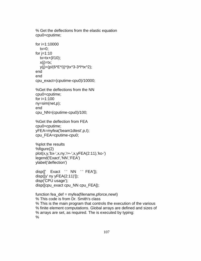
107
% Get the deflections from the elastic equation cpu0=cputime; for i=1:10000 tx=0; for j=1:10 tx=tx+(l/10); x(j)=tx; y(j)=(p/(6*E*I))*(tx^3-3*l*tx^2); end end cpu_exact=(cputime-cpu0)/10000; %Get the deflections from the NN cpu0=cputime; for i=1:100 ny=sim(net,p); end cpu_NN=(cputime-cpu0)/100; %Get the deflection from FEA cpu0=cputime; yFEA=myfea('beam1dtest',p,I); cpu_FEA=cputime-cpu0; %plot the results %figure(2) plot(x,y,'bx-',x,ny,'r+-',x,yFEA(2:11),'ko-') legend('Exact','NN','FEA') ylabel('deflection') disp([' Exact ' ' NN ' ' FEA']); disp([y' ny yFEA(2:11)']); disp('CPU usage'); disp([cpu_exact cpu_NN cpu_FEA]); function fea_def = myfea(filename,pforce,newI) % This code is from Dr. Smith's class % This is the main program that controls the execution of the various % finite element computations. Global arrays are defined and sizes of % arrays are set, as required. The is executed by typing: %

108
% >> myfea('filename') % % at the MATLAB prompt where 'filename' refers to the input file named % filename.txt in the current directory. This program calls all of the % functions needed to run a finite element simulation. It also contains % the calculations that invert the global reduced stiffness matrix and % performs the back substitution step that computes the unknown nodal % degrees-of-freedom. Reaction loads are then computed. % % define global arrays %yFEA is the solution global ielem iprops eprops elname iforce force idisp disp global kff kpf kpp uf up pf pp yFEA global x utot estress efor etype shear moment xplot % %close all graphs close all % % assign input filename filename = [filename '.txt']; % % read input file [nnode,nel,nforce,ndisp,etype,ndof,nenode]=fea_input(filename); % %print input values to screen %[nnode nel nforce ndisp etype ndof nenode] % % initialize equation numbers for dofs ieqn = initialize(nnode,ndisp,idisp,ndof); % % initialize global matrices; utot=zeros(nnode*ndof,1); ptot=zeros(nnode*ndof,1); kff = zeros(nnode*ndof-ndisp); kpf = zeros(ndisp,nnode*ndof-ndisp); kpp = zeros(ndisp,ndisp); uf = zeros(nnode*ndof-ndisp,1); up = disp'; pf = zeros(nnode*ndof-ndisp,1); pp = zeros(ndisp,1); estress = zeros(nel,1); efor = zeros(nel,1);

109
eprops(1,2)=newI; % % compute and assemble element stiffness matrix and draw geometry % figure(1) % title('Model') % xlabel('X'), ylabel('Y'), zlabel('Z') % hold('on') % grid('on') XYZ=zeros(nel,3); for i = 1:nel; icode = 2; XYZ(1,:)=x(ielem(i,1),:); XYZ(2,:)=x(ielem(i,2),:); %plot3(XYZ(:,1),XYZ(:,2),XYZ(:,3),'k') [eldat,ieleqn] = feval(elname,eprops(iprops(i),:),ielem(i,1:2),ieqn,icode,i); assemkp(eldat,ieleqn,ndof,nenode,icode); end % % compute and assemble element load vector for i = 1:nel; icode = 1; [eldat,ieleqn] = feval(elname,eprops(iprops(i),:),ielem(i,1:2),ieqn,icode,i); assemkp(eldat,ieleqn,ndof,nenode,icode); end % % apply nodal forces force=-pforce; for i = 1:nforce; num = iforce(i,1)*ndof + iforce(i,2) - ndof; pf(ieqn(num)) = pf(ieqn(num)) + force(i); end % % solve system of equations uf = kff\(pf - kpf'*up); % % compute nodal reactions pp = kpp*up + kpf*uf; % % complete global displacement and force vector % for i = 1:nnode*ndof; if (ieqn(i) < 0);

110
utot(i,1) = up(-ieqn(i)); ptot(i,1) = pp(-ieqn(i)); else utot(i,1) = uf(ieqn(i)); ptot(i,1) = pf(ieqn(i)); end end % %postprocess for i = 1:nel icode = 0; [eldat,ieleqn] = feval(elname,eprops(iprops(i),:),ielem(i,1:2),ieqn,icode,i); shear(i)=(eldat(1)-eldat(3))/2; moment(i)=(-eldat(2)+eldat(4))/2; xplot(i)=(x(i)+x(i+1))/2; end fea_output(etype,utot,ptot,nnode); fea_def=yFEA; function ieqn = initialize(nnode,ndisp,idisp,ndof) % % This function is used to count the number of equations in the model and % assign element equation numbers. Equation numbers increase from zero for % free dofs and decrease from zero for prescribed dofs. % %set total degrees of freedom ndoftot = nnode*ndof; % % initialize ieqn ieqn = zeros(1,ndoftot); % % identify fixed degrees of freedom ifixed = 0; for i = 1:ndisp; ifixed = ifixed + 1; num = idisp(i,1)*ndof + idisp(i,2) - ndof; ieqn(num) = -ifixed; end % % identify free degrees of freedom ifree = 0; for i = 1:ndoftot; if ieqn(i) == 0;

111
ifree = ifree + 1; ieqn(i) = ifree; end end function [nnode,nel,nforce,ndisp,etype,ndof,nenode] = fea_input(filename) % % This function reads the input file filename.txt in the current directory. % It starts by reading the number of nodes, elements, applied loads, % prescribed displacements and element type. It then reads nodal data, % element data, load data, prescribed displacement data and finally, the % element properties. The number of nodal dofs, nodes per element, and % number of element properties are also assigned for each element type. % %define global arrays global ielem iprops eprops elname iforce force idisp disp global x knl DV DVid % % open input file fid = fopen(filename,'r'); % % read number of nodes, elements, applied forces and prescribed displacements, and element type nnode = fscanf(fid,'%d',1); nel = fscanf(fid,'%d',1); nforce = fscanf(fid,'%d',1); ndisp = fscanf(fid,'%d',1); etype = fscanf(fid,'%d',1); %[nnode nel nforce ndisp etype ndof nenode] % set properties related to element properties % set knl to non-linear default knl = 0; switch etype case 1 ndof = 1; nenode = 2; neprops = 1; elname = 'spring1d'; case 2 ndof = 2; nenode = 2; neprops = 2; elname = 'truss2d';

112
case 3 knl = 1; ndof =1; nenode = 2; neprops = 3; elname = 'spring1d_nl'; case 4 ndof = 2; nenode = 2; neprops = 3; elname = 'beam1d'; end % % read nodal data x = zeros(nnode,3); for j = 1:nnode; dummy = fscanf(fid,'%d',1); x(j,1:3) = fscanf(fid,'%g',3)'; end % % read element data ielem = zeros(nel,nenode); iprops = zeros(1,nel); for j = 1:nel; fscanf(fid,'%d',1); iprops(j) = fscanf(fid,'%d',1); ielem(j,1:nenode); ielem(j,1:nenode) = fscanf(fid,'%d',nenode)'; end % % read applied loads iforce = zeros(nforce,2); force = zeros(1,nforce); for j = 1:nforce; iforce(j,1:2) = fscanf(fid,'%d',2)'; force(j) = fscanf(fid,'%g',1); end % % read applied displacements idisp = zeros(ndisp,2); disp = zeros(1,ndisp); for j = 1:ndisp idisp(j,1:2) = fscanf(fid,'%d',2)';

113
disp(j) = fscanf(fid,'%g',1); end % % read element properties nprops = max(iprops); eprops = zeros(nprops,neprops); for j = 1:nprops; fscanf(fid,'%d',1); eprops(j,1:neprops) = fscanf(fid,'%g',neprops)'; end % % design sensitivity analysis DV=fscanf(fid,'%d',1); for j=1:DV; DVid(j,1:2)=fscanf(fid,'%d',1); end % function fea_output(etype,utot,ptot,nnode) % % This function is used to output finite element results to the % MATLAB window or, perhaps, to a file (not included here). % % print the following to the screen % calculates system compliance for springs % prints element force and stress for rods global efor estress shear moment xplot x yFEA switch etype case 1,3 syscomp=dot(utot,ptot) case 2 efor estress case 4 X=zeros(nnode,1); %disp(sprintf('number of nodes: %i',nnode)); for i=1:nnode; deflection(i)=utot(i*2-1); slope(i)=utot(i*2); X(i)=x(i,1); if i==(nnode+1)/2 %disp(sprintf('theta 2=%0.4g ',slope(i))); end

114
end %disp(sprintf('max deflection=%0.4g',(max(abs(deflection))))); yFEA=deflection; % figure(2) % title('Moment') % hold('on') % plot(xplot,moment,'b') % figure(3) % title('Shear') % hold('on') % plot(xplot,shear,'g') % figure(4) % title('deflection') % hold('on') % plot(X,deflection,'r') End function [eldat,ieleqn] = beam1d(eprop,lnodes,ieqn,icode,i) % % This function computes the element load vector (case 1) and % element stiffness matrix (case 2) for a 1-D beam element. Note % that the element load vector is zero. It starts by forming the % element equation numbers that are required to assemble the global % matrices. global x utot estress efor % %determine length, sin, and cos i1x=x(lnodes(1),:); i2x=x(lnodes(2),:); L=abs(i2x(1)-i1x(1)); k=[6 3*L -6 3*L;3*L 2*L^2 -3*L L^2;-6 -3*L 6 -3*L;3*L L^2 -3*L 2*L^2]; nenode = 2; ndof = 2; jj = 0; for j1 = 1:nenode; for j2 = 1:ndof; jj = jj + 1; numj = lnodes(j1)*ndof + j2 - ndof; idof(jj,1)=numj; ieleqn(jj) = ieqn(numj); if icode==0

115
euv(jj)=utot(numj); end end end % % evaluate element matrices uloc=utot(idof(:,1)); switch icode case 0 %postprocess: moment and shear eldat = ((eprop(1)*eprop(2)*2)/L^3)*k*uloc-(eprop(3)*L/2)*[1;L/6;1;-L/6]; case 1 % compute element load vector eldat = (eprop(3)*L/2)*[1;L/6;1;-L/6]; case 2 % compute element stiffness matrix eldat = ((eprop(1)*eprop(2)*2)/L^3)*k; end

116
Appendix C: MATLAB Program For DSO of Typical MMT Base Side %*********Continous Constrained Optimization % for typical 2D MMT Base Side % this program generates all of the branches % and finds the continous optimal solution % for each branch and save them to a file %---------------------------------------------- clear all close all global X b h d enac num_ele nn_save nu_sol nu_fea P T LOAD nn_save=0; nu_sol=0; nu_fea=1; b=36; h=12; d=12; X=zeros(4,3); X(2,2)=h; X(4,2)=h; X(3,3)=d; X(4,3)=d; LOAD=[2 2 75; 3 2 -700]; enac=6; % number of elements across the top % set the number of extra elements num_ele=0; %set optimazation options % options = optimset('LargeScale','off','DiffMaxChange',.5,'DiffMinChange',0.005,'Diagnostics','off','Display','off','TolFun',0.1,'TolCon',0.01,'TolX',0.05); options = optimset('LargeScale','off','DiffMaxChange',1,'DiffMinChange',0.005,'Diagnostics','off','Display','off','TolFun',2.0,'TolCon',0.01,'TolX',0.1); %% optimize with no extra elements LB = zeros(8,1); UB = ones(8,1); %test worst case for feasible solution if mynonlin_cons_2d(UB) <= 0 clear P T; global P T

117
P=zeros(100,13); T=zeros(100,7); nu_fea=1; nn_save=1; nu_sol=nu_sol+1 mynonlin_cons_2d(UB); mynonlin_cons_2d(LB); x0=mypso2d(LB); x0=x0'; % options = optimset('LargeScale','off','DiffMaxChange',.5,'DiffMinChange',0.005,'Diagnostics','off','Display','off','TolFun',0.1,'TolCon',0.01,'TolX',0.05); [fx, fval, exitflag, output, lambda] = fmincon('obj_2d',x0,[],[],[],[],LB,UB,'mynonlin_cons_2d',options); xtemp=[X(1,1) X(2,1) X(3,1) X(4,1)]; save(strcat('X',num2str(nu_sol)),'X','-ascii'); save(strcat('P',num2str(nu_sol)),'P','-ascii'); save(strcat('T',num2str(nu_sol)),'T','-ascii'); sol(nu_sol)=fval; nn_save=0; end %% end no extra elements %% optimize with one extra elements % set the number of extra elements num_ele=1; clear x0 UB LB; LB = zeros(10,1); UB = ones(10,1); X(1,1)=0;X(2,1)=0;X(3,1)=0;X(4,1)=0; for xi=1:(enac+1) X(1,1)=0; for xj=1:(enac+1) %test worst case for feasible solution if mynonlin_cons_2d(UB) <= 0 clear P T; global P T P=zeros(100,13); T=zeros(100,7); nu_fea=1;

118
nn_save=1; nu_sol=nu_sol+1 mynonlin_cons_2d(UB); mynonlin_cons_2d(LB); x0=mypso2d(LB); x0=x0'; %x0=LB+.5; % options = optimset('LargeScale','off','DiffMaxChange',.5,'DiffMinChange',0.005,'Diagnostics','off','Display','off','TolFun',0.1,'TolCon',0.01,'TolX',0.05); [fx, fval, exitflag, output, lambda] = fmincon('obj_2d',x0,[],[],[],[],LB,UB,'mynonlin_cons_2d',options); xtemp=[X(1,1) X(2,1) X(3,1) X(4,1)]; save(strcat('X',num2str(nu_sol)),'X','-ascii'); save(strcat('P',num2str(nu_sol)),'P','-ascii'); save(strcat('T',num2str(nu_sol)),'T','-ascii'); sol(nu_sol)=fval; nn_save=0; end X(1,1)=X(1,1)+b/enac; end X(2,1)=X(2,1)+b/enac; end X(1,1)=0;X(2,1)=0;X(3,1)=0;X(4,1)=0; %save the solutions save sol.txt sol -ascii; function pbest=mypso2d(L) % this function uses particle swarm to optimize the %continous branch of a typical MMT Base Side % this is the 2D version global X b h d enac num_ele nn_save nu_sol P T nu_fea LOAD %pass the following to the function once it works wmax=0.9; wmin=0.4; itmax=8; errmax=.0001; c1=2; c2=2;

119
N=50; D=size(L,1); i=1:itmax; W=wmax-((wmax-wmin)/itmax)*i; % Initialization of positions a=0; b=1; x=a+(b-a)*rand(N,D,1); for i=1:N F(i,1)=myext_penalty2d(x(i,:)'); end [C,I]=min(abs(F(:,1))); pB=C; gB=pB; XX(1,1)=I; gbest(1,:)=x(I,:); pbest=gbest; for i=1:N V=c1*rand*(pbest-x(i,:))+c2*rand*(gbest-x(i,:)); x(i,:)=x(i,:)+V; end jj=0; while jj<itmax for i=1:N x(i,:)=myclamped(x(i,:),0,1); F(i,1)=myext_penalty2d(x(i,:)'); end [C,I]=min(abs(F(:,1))); gbest(1,:)=x(I,:); gB=C; for i=1:N V=W(jj+1)*c1*rand*(pbest-x(i,:))+c2*rand*(gbest-x(i,:)); x(i,:)=x(i,:)+V; end

120
if gB<pB pB=gB; pbest=gbest; end jj=jj+1; %sol(jj,1:(D+1))=[pB pbest']; end function [c, ceq] = mynonlin_cons_2d(L) % this function take cross sectional data L2 and t % and returns the deflection and 1st natural freq of the % structure % global X b h d enac num_ele nn_save nu_sol P T nu_fea LOAD %remove the following after testing b=36; h=12; d=12; enac=6; nenode=2;% nenode = number of nodes/element ndof=6;% ndof=number of degrees of freedom/node %mesh the model [x, ielem]=mymesh2d; %get element properties eleprop=myeleprop2d(L); nnode=size(x,1);% nnode=total number of nodes nel=size(ielem,1);% nel=total number of elements % %set BC and loads BC=zeros(nnode,ndof); %zero=free 1=fixed BC([enac+2 (enac+1)*2],1:6)=1; %BC([enac+2 tot_ele+2],1:6)=1; BC(1:nnode,3:5)=1; F(1:nnode*ndof)=0; XYZ=zeros(nel,3);

121
K=zeros(nnode*ndof,nnode*ndof); M=zeros(nnode*ndof,nnode*ndof); %element and cs data for book example delete for final % use the Lsection program to replace % Set up all the constants E=30e6; G=11.5e6; rho=0.286; %get element stiffness matrices then put in global stiffness matrix % set the lumped mass matrix for i = 1:nel; A=eleprop(i,1); Iy=eleprop(i,2); Iz=eleprop(i,3); J=eleprop(i,4); k=mystiff(E,G,A,Iy,Iz,J,x(ielem(i,1),1),x(ielem(i,1),2),x(ielem(i,1),3),x(ielem(i,2),1),x(ielem(i,2),2),x(ielem(i,2),3)); m=mymass(rho,A,x(ielem(i,1),1),x(ielem(i,1),2),x(ielem(i,1),3),x(ielem(i,2),1),x(ielem(i,2),2),x(ielem(i,2),3)); M=myassemble(M,m,ielem(i,1),ielem(i,2)); K=myassemble(K,k,ielem(i,1),ielem(i,2)); end % compute and assemble element load vector force vector i2=1;i3=1; for i = 1:nnode;%loop thru each node for i1=1:ndof;%loop thru each dof in the node if BC(i,i1) == 0; %set up book keeping for partition bk(i3)=i2; i3=i3+1; end i2=i2+1; end end % Insert forces into global force vector for i=1:size(LOAD,1); F((LOAD(i,1)-1)*6+LOAD(i,2))=LOAD(i,3); end

122
%partition the system of eq. m=zeros(size(bk,2),size(bk,2)); k=zeros(size(bk,2),size(bk,2)); f(1:size(bk,2))=0; for i=1:size(bk,2); for i1=1:size(bk,2); m(i,i1)=M(bk(i),bk(i1)); k(i,i1)=K(bk(i),bk(i1)); end f(i)=F(bk(i)); end % %solve for 1st natural frequency w=eig(k,m); w1=sqrt(abs(w(1))); %solve for displacements u=k\f'; %Setup Global Nodal Displacement Vector U(1:nnode*ndof)=0; for i=1:size(bk,2); U(bk(i))=u(i); end %calculate the global nodal force vector F=K*U'; %set max deflection and natural freq. md=0.005;mf=40; % nonlinear inequality constraints returned as vector c for i=1:(enac+1) ydisp(i)=U((i-1)*6+2); % ydisp(i+(enac+1))=U(((i+(2*enac+3))-2)*6+2); end if nn_save==1 temp=zeros(13,1); temp(2:size(L,1)+1,1)=L; temp(1,1)=num_ele; P(nu_fea,:)=temp';

123
T(nu_fea,:)=ydisp; nu_fea=nu_fea+1; clear temp; end c=max(abs(ydisp))-md; % nonlinear equality constraints returned as vector ceq ceq = []; % there are no nonlinear equality % constraints in this problem function [c, ceq] = myext_penalty2d(L) % this function take cross sectional data L2 and t % and returns the deflection and natural freq of the % structure %******** This uses external penalty function %********** used for the PSO because it is %********* unconstrained % global X b h d enac num_ele nn_save nu_sol P T nu_fea LOAD %remove the following after testing b=36; h=12; d=12; enac=6; volume=obj_2d(L); nenode=2;% nenode = number of nodes/element ndof=6;% ndof=number of degrees of freedom/node vl=size(L,1); L2=L(1:vl/2)*1.25+0.75; t=L(vl/2+1:vl)*.375+.125; %mesh the model [x, ielem]=mymesh2d; %get element properties eleprop=myeleprop2d(L); nnode=size(x,1);% nnode=total number of nodes nel=size(ielem,1);% nel=total number of elements %

124
%set BC and loads BC=zeros(nnode,ndof); %zero=free 1=fixed BC([enac+2 (enac+1)*2],1:6)=1; BC(1:nnode,3:5)=1; F(1:nnode*ndof)=0; XYZ=zeros(nel,3); K=zeros(nnode*ndof,nnode*ndof); M=zeros(nnode*ndof,nnode*ndof); %element and cs data for book example delete for final % use the Lsection program to replace % Set up all the constants E=30e6; G=11.5e6; rho=0.286; %get element stiffness matrices then put in global stiffness matrix % set the lumped mass matrix for i = 1:nel; A=eleprop(i,1); Iy=eleprop(i,2); Iz=eleprop(i,3); J=eleprop(i,4); k=mystiff(E,G,A,Iy,Iz,J,x(ielem(i,1),1),x(ielem(i,1),2),x(ielem(i,1),3),x(ielem(i,2),1),x(ielem(i,2),2),x(ielem(i,2),3)); m=mymass(rho,A,x(ielem(i,1),1),x(ielem(i,1),2),x(ielem(i,1),3),x(ielem(i,2),1),x(ielem(i,2),2),x(ielem(i,2),3)); M=myassemble(M,m,ielem(i,1),ielem(i,2)); K=myassemble(K,k,ielem(i,1),ielem(i,2)); end % compute and assemble element load vector force vector i2=1;i3=1; for i = 1:nnode;%loop thru each node for i1=1:ndof;%loop thru each dof in the node if BC(i,i1) == 0; %set up book keeping for partition

125
bk(i3)=i2; i3=i3+1; end i2=i2+1; end end % Insert forces into global force vector for i=1:size(LOAD,1); F((LOAD(i,1)-1)*6+LOAD(i,2))=LOAD(i,3); end %partition the system of eq. m=zeros(size(bk,2),size(bk,2)); k=zeros(size(bk,2),size(bk,2)); f(1:size(bk,2))=0; for i=1:size(bk,2); for i1=1:size(bk,2); m(i,i1)=M(bk(i),bk(i1)); k(i,i1)=K(bk(i),bk(i1)); end f(i)=F(bk(i)); end % %solve for 1st natural frequency w=eig(k,m); w1=sqrt(abs(w(1))); %solve for displacements u=k\f'; %Setup Global Nodal Displacement Vector U(1:nnode*ndof)=0; for i=1:size(bk,2); U(bk(i))=u(i); end %calculate the global nodal force vector F=K*U'; %set max deflection and natural freq. md=0.005;mf=40; % nonlinear inequality constraints returned as vector c

126
%Get the y disp for the top surface for i=1:(enac+1) ydisp(i)=U((i-1)*6+2); end if nn_save==1 temp=zeros(13,1); temp(2:size(L,1)+1,1)=L; temp(1,1)=num_ele; P(nu_fea,:)=temp'; T(nu_fea,:)=ydisp; nu_fea=nu_fea+1; clear temp; end % external penaly function c=volume + 5000*(max(abs(ydisp))-md)^2; % nonlinear equality constraints returned as vector ceq ceq = []; % there are no nonlinear equality % constraints in this problem function = discrete_2d() % this function loads the branch data from the continous optimization % It test the best topos and cuts branches. Can either do NN or FEA % If NN it can load previous weights and bias or generate new. clear all close all global X b h d enac num_ele nn_save nu_sol nu_fea P T LOAD nn_save=0; %** set hidden layer size factor hls=1.5; %*** get input from user pretrain=input('pretrain NN? 1=yes 0=no'); useNN=input('use NN? 1=yes 0=no'); LOAD=[2 2 75; 3 2 -700]; nu_sol=0; nu_fea=1; enac=6; % number of elements across the top % set the number of extra elements

127
num_ele=1; %load and sort the continuous sol. for each branch load sol.txt -ascii; [Y,I]=sort(sol); sol_temp=10000; j=1; cpu_seconds=0; while sol_temp>sol(j) i=I(j); p=load(strcat('P',num2str(i)),'-ascii'); t=load(strcat('T',num2str(i)),'-ascii'); topo=load(strcat('X',num2str(i)),'-ascii'); P=p'; T=t'; X=topo clear t p topo; if useNN == 1 %*** test if NN ***** % ************ build NN and train ****************** minP=min(P'); maxP=max(P'); PR=[minP',maxP']; layer1=round(1.5*size(P,1)); layer2=round(layer1/2); outlayer=size(T,1); %net = newff(PR,[layer1 outlayer],{'logsig','tansig'},'traincgf'); net = newff(PR,[layer1 layer2 outlayer],{'tansig', 'logsig','purelin'},'trainrp'); %net.trainParam.mem_reduc=4; net.trainParam.goal=1e-6; net.trainParam.show=100; net.trainParam.epochs=2000; if pretrain > 0 % load prevous NN weights and bias load -ascii pw1.txt;net.IW{1,1}=pw1; load -ascii pw2.txt;net.LW{2,1}=pw2; load -ascii pw3.txt;net.LW{3,2}=pw3; load -ascii pb1.txt;net.b{1,1}=pb1; load -ascii pb2.txt;net.b{2,1}=pb2; load -ascii pb3.txt;net.b{3,1}=pb3; net = newff(PR,[layer1 layer2 outlayer],{'tansig', 'logsig','purelin'},'trainlm');

128
net.trainParam.goal=1e-10; net.trainParam.epochs=150; end %***** end pretrain ***** %**** train network ****** net=train(net,P,T); pretrain=2;%***** use pretrained data for future test *** %********** finish build and train the NN ***************** % save the weights and bias for later w1=net.IW{1,1}; w2=net.LW{2,1}; w3=net.LW{3,2}; b1=net.b{1,1}; b2=net.b{2,1}; b3=net.b{3,1}; save pw1.txt w1 -ascii; save pw2.txt w2 -ascii; save pw3.txt w3 -ascii; save pb1.txt b1 -ascii; save pb2.txt b2 -ascii; save pb3.txt b3 -ascii; end %********* end NN test ********** %******* test each branch ************ k=0; cpu0=cputime; for k1=1:3 for k2=1:3 for k3=1:3 for k4=1:3 for k5=1:3 L=[k1; k2; k3; k4; k5]; temp=zeros(13,1); dL=dlsection(L); temp(2:size(dL,1)+1,1)=dL; temp(1,1)=num_ele; if useNN == 1 ydisp=sim(net,temp); else

129
ydisp = fea_2d_test(dL)'; end k=k+1; if max(abs(ydisp))<=.009 sol_temp1=obj_2d(dL); if sol_temp1<sol_temp sol_temp=sol_temp1; sol_dL=dL; dX=X; sol_disp=ydisp; end end end end end end end j=j+1; cpu1=cputime;cpu_seconds=cpu_seconds+(cpu1-cpu0) end %end the while %plot final topo. X=dX [x, ielem]=mymesh2d; nnode=size(x,1);% nnode=total number of nodes nel=size(ielem,1);% nel=total number of elements figure(1) title('Model') xlabel('X'), ylabel('Y'), zlabel('Z') hold('on') grid('on') XYZ=zeros(nel,3); for i = 1:nel; XYZ(1,1:3)=x(ielem(i,1),1:3); XYZ(2,1:3)=x(ielem(i,2),1:3); plot3(XYZ(1:2,1),XYZ(1:2,2),XYZ(1:2,3),'k') end sol_temp

130
sol_dL k nload=size(LOAD,1); i11=0; for i1=1:nload if LOAD(i1,2)==1, i11=i11+1; load(i11,1:3)=[LOAD(i1,3),0,0]; y(i11)=i1; elseif LOAD(i1,2)==2, i11=i11+1; load(i11,1:3)=[0,LOAD(i1,3),0]; y(i11)=i1; elseif LOAD(i1,2)==3, i11=i11+1; load(i11,1:3)=[0,0,LOAD(i1,3)]; y(i11)=i1; end end if i11>=1, x=[1:i11]; quiver3(LOAD(y,1)*6-6,[12; 12],[0; 0],load(x,1),load(x,2),load(x,3),'r') end %% end one extra elements

131
Appendix D: MATLAB Program – Material Distribution Topology Optimization %******* Modified by Donald Harby for testing typical MMT Base Sides 2D*** %%%% A 99 LINE TOPOLOGY OPTIMIZATION CODE BY OLE SIGMUND, JANUARY 2000 %%% %%%% CODE MODIFIED FOR INCREASED SPEED, September 2002, BY OLE SIGMUND %%% %******* Modified for MMT base 8-21-07 Donald Harby *** function topo() clear all nelx=72;nely=24;volfrac=0.4;penal=2.5;rmin=1.1; close all hold off % INITIALIZE x(1:nely,1:nelx) = volfrac; %**** Add fixed material and holes *** % ****** passive holes active fixed material ** for ely=1:nely for elx=1:nelx active(ely,elx)=0; if elx<=2 active(ely,elx)=1; x(ely,elx)=1; end if elx>=nelx-1 active(ely,elx)=1; x(ely,elx)=1; end if ely<=2 active(ely,elx)=1; x(ely,elx)=1; end if ely>=nely-1 active(ely,elx)=1; x(ely,elx)=1; end end

132
end %********* end my passive or active loop = 0; change = 1.; % START ITERATION % while change > 0.01 while loop < 60 loop = loop + 1; xold = x; % FE-ANALYSIS [U]=FE(nelx,nely,x,penal); % OBJECTIVE FUNCTION AND SENSITIVITY ANALYSIS [KE] = lk; c = 0.; for ely = 1:nely for elx = 1:nelx n1 = (nely+1)*(elx-1)+ely; n2 = (nely+1)* elx +ely; dc(ely,elx)=0.; for i=1:2 Ue = U([2*n1-1;2*n1; 2*n2-1;2*n2; 2*n2+1;2*n2+2; 2*n1+1;2*n1+2],i); c = c + x(ely,elx)^penal*Ue'*KE*Ue; dc(ely,elx) = dc(ely,elx)-penal*x(ely,elx)^(penal-1)*Ue'*KE*Ue; end end end % FILTERING OF SENSITIVITIES [dc] = check(nelx,nely,rmin,x,dc); % DESIGN UPDATE BY THE OPTIMALITY CRITERIA METHOD [x] = OC(nelx,nely,x,volfrac,dc,active); % PRINT RESULTS change = max(max(abs(x-xold))); disp([' It.: ' sprintf('%4i',loop) ' Obj.: ' sprintf('%10.4f',c) ... ' Vol.: ' sprintf('%6.3f',sum(sum(x))/(nelx*nely)) ... ' ch.: ' sprintf('%6.3f',change )]) % PLOT DENSITIES colormap(gray); imagesc(-x); axis equal; axis tight; axis off;pause(1e-6); end %plot load vector hold on quiver3(72*2/6,0,0,0,10,0,'r') quiver3(72*2/6-12,5,0,0,-1,0,.7,'g')

133
%%%%%%%%%% OPTIMALITY CRITERIA UPDATE %%%%%%%%%%%%%%%%%%%%%%%%%%%%%%%%%%%%%% function [xnew]=OC(nelx,nely,x,volfrac,dc,active) l1 = 0; l2 = 100000; move = 0.2; while (l2-l1 > 1e-4) lmid = 0.5*(l2+l1); xnew = max(0.001,max(x-move,min(1.,min(x+move,x.*sqrt(-dc./lmid))))); xnew(find(active))=1.0; if sum(sum(xnew)) - volfrac*nelx*nely > 0; l1 = lmid; else l2 = lmid; end end %%%%%%%%%% MESH-INDEPENDENCY FILTER %%%%%%%%%%%%%%%%%%%%%%%%%%%%%%%%%%%%%%%% function [dcn]=check(nelx,nely,rmin,x,dc) dcn=zeros(nely,nelx); for i = 1:nelx for j = 1:nely sum=0.0; for k = max(i-floor(rmin),1):min(i+floor(rmin),nelx) for l = max(j-floor(rmin),1):min(j+floor(rmin),nely) fac = rmin-sqrt((i-k)^2+(j-l)^2); sum = sum+max(0,fac); dcn(j,i) = dcn(j,i) + max(0,fac)*x(l,k)*dc(l,k); end end dcn(j,i) = dcn(j,i)/(x(j,i)*sum); end end %%%%%%%%%% FE-ANALYSIS %%%%%%%%%%%%%%%%%%%%%%%%%%%%%%%%%%%%%%%%%%%%%%%%%%%%% function [U]=FE(nelx,nely,x,penal) [KE] = lk; K = sparse(2*(nelx+1)*(nely+1), 2*(nelx+1)*(nely+1)); F = sparse(2*(nely+1)*(nelx+1),2); U = zeros(2*(nely+1)*(nelx+1),2); for elx = 1:nelx

134
for ely = 1:nely n1 = (nely+1)*(elx-1)+ely; n2 = (nely+1)* elx +ely; edof = [2*n1-1; 2*n1; 2*n2-1; 2*n2; 2*n2+1; 2*n2+2; 2*n1+1; 2*n1+2]; K(edof,edof) = K(edof,edof) + x(ely,elx)^penal*KE; end end % DEFINE LOADS AND SUPPORTS (HALF MBB-BEAM) % F(2,1) = -1; % fixeddofs = union([1:2:2*(nely+1)],[2*(nelx+1)*(nely+1)]); %**** my forces and BC Donald Harby mid_x=round(2*nelx/6); F(2*(mid_x)*(nely+1)+2,1)=-1; F(2*(mid_x-12)*(nely+1)+2,2)=.25; fixeddofs=[2*(nely+1)-1 2*(nely+1) 2*(nelx+1)*(nely+1)-1 2*(nelx+1)*(nely+1)]; %*************** alldofs = [1:2*(nely+1)*(nelx+1)]; freedofs = setdiff(alldofs,fixeddofs); % SOLVING U(freedofs,:) = K(freedofs,freedofs) \ F(freedofs,:); U(fixeddofs,:)= 0; %%%%%%%%%% ELEMENT STIFFNESS MATRIX %%%%%%%%%%%%%%%%%%%%%%%%%%%%%%%%%%%%%%%% function [KE]=lk E = 1.; nu = 0.3; k=[ 1/2-nu/6 1/8+nu/8 -1/4-nu/12 -1/8+3*nu/8 ... -1/4+nu/12 -1/8-nu/8 nu/6 1/8-3*nu/8]; KE = E/(1-nu^2)*[ k(1) k(2) k(3) k(4) k(5) k(6) k(7) k(8) k(2) k(1) k(8) k(7) k(6) k(5) k(4) k(3) k(3) k(8) k(1) k(6) k(7) k(4) k(5) k(2) k(4) k(7) k(6) k(1) k(8) k(3) k(2) k(5) k(5) k(6) k(7) k(8) k(1) k(2) k(3) k(4) k(6) k(5) k(4) k(3) k(2) k(1) k(8) k(7) k(7) k(4) k(5) k(2) k(3) k(8) k(1) k(6) k(8) k(3) k(2) k(5) k(4) k(7) k(6) k(1)]; % %%%%%%%%%%%%%%%%%%%%%%%%%%%%%%%%%%%%%%%%%%%%%%%%%%%%%%%%%%%%%%%%%%%%%%%%%%%% % This Matlab code was written by Ole Sigmund, Department of Solid %

135
% Mechanics, Technical University of Denmark, DK-2800 Lyngby, Denmark. % % Please sent your comments to the author: [email protected] % % % % The code is intended for educational purposes and theoretical details % % are discussed in the paper % % "A 99 line topology optimization code written in Matlab" % % by Ole Sigmund (2001), Structural and Multidisciplinary Optimization, % % Vol 21, pp. 120--127. % % % % The code as well as a postscript version of the paper can be % % downloaded from the web-site: http://www.topopt.dtu.dk % % % % Disclaimer: % % The author reserves all rights but does not guaranty that the code is % % free from errors. Furthermore, he shall not be liable in any event % % caused by the use of the program. % %%%%%%%%%%%%%%%%%%%%%%%%%%%%%%%%%%%%%%%%%%%%%%%%%%%%%%%%%%%%%%%%%%%%%%%%%%%%

136
Appendix E: MATLAB Program PSO of MMT Base 3D %*********Continous Constrained Optimization % Test and generates the branches for the 3D case % of a typical MMT Base structure % Saves the data for NN testing %---------------------------------------------- clear all close all global X b h d enac num_ele nn_save nu_sol nu_fea P T LOAD LOAD=[5 2 100; 6 2 -1200;19 2 -1200;20 2 100]; nn_save=0; nu_sol=0; nu_fea=1; b=36; h=12; d=12; X=zeros(4,3); X(2,2)=h; X(4,2)=h; X(3,3)=d; X(4,3)=d; enac=6; % number of elements across the top % set the number of extra elements num_ele=0; %set optimazation options % options = optimset('LargeScale','off','DiffMaxChange',.5,'DiffMinChange',0.005,'Diagnostics','off','Display','off','TolFun',0.1,'TolCon',0.01,'TolX',0.05); options = optimset('LargeScale','off','DiffMaxChange',1,'DiffMinChange',0.005,'Diagnostics','off','Display','off','TolFun',2.0,'TolCon',0.01,'TolX',0.1); %% optimize with no extra elements LB = zeros(24,1); UB = ones(24,1); %test worst case for feasible solution if mynonlin_cons_1(UB) <= 0 nn_save=1; nu_sol=nu_sol+1; disp('foo') % x0=mypso;

137
x0=LB+.5; % options = optimset('LargeScale','off','DiffMaxChange',.5,'DiffMinChange',0.005,'Diagnostics','off','Display','off','TolFun',0.1,'TolCon',0.01,'TolX',0.05); [fx, fval, exitflag, output, lambda] = fmincon('obj_3d_1',x0,[],[],[],[],LB,UB,'mynonlin_cons_1',options); nn_save=0; end %% end no extra elements %% optimize with one extra elements % set the number of extra elements num_ele=1; clear x0 UB LB; LB = zeros(26,1); UB = ones(26,1); for xi=1:(enac+1) X(1,1)=0; for xj=1:(enac+1) %test worst case for feasible solution if mynonlin_cons_1(UB) <= 0 nn_save=1; nu_sol=nu_sol+1; disp('foo2') % x0=mypso; x0=LB+.5; % options = optimset('LargeScale','off','DiffMaxChange',.5,'DiffMinChange',0.005,'Diagnostics','off','Display','off','TolFun',0.1,'TolCon',0.01,'TolX',0.05); %[fx, fval, exitflag, output, lambda] = fmincon('obj_3d_1',x0,[],[],[],[],LB,UB,'mynonlin_cons_1',options); nn_save=0; end X(1,1)=X(1,1)+b/enac; end X(2,1)=X(2,1)+b/enac; end X(1,1)=0;X(2,1)=0; %% end one extra elements

138
%% optimize with two extra elements % set the number of extra elements num_ele=2; clear x0 UB LB; LB = zeros(28,1); UB = ones(28,1); for xi=1:(enac+1) X(1,1)=0; for xj=1:(enac+1) X(3,1)=0; for xii=1:(enac+1) X(4,1)=0; for xjj=1:(enac+1) %test worst case for feasible solution if mynonlin_cons_1(UB) <= 0 clear P T; global P T P=zeros(100,28); T=zeros(100,14); nu_fea=1; nn_save=1; nu_sol=nu_sol+1 x0=mypso(LB); x0=x0'; mynonlin_cons_1(UB); mynonlin_cons_1(LB); %x0=LB+.5; % options = optimset('LargeScale','off','DiffMaxChange',.5,'DiffMinChange',0.005,'Diagnostics','off','Display','off','TolFun',0.1,'TolCon',0.01,'TolX',0.05); [fx, fval, exitflag, output, lambda] = fmincon('obj_3d_1',x0,[],[],[],[],LB,UB,'mynonlin_cons_1',options); xtemp=[X(1,1) X(2,1) X(3,1) X(4,1)]; save(strcat('X',num2str(nu_sol)),'X','-ascii'); save(strcat('P',num2str(nu_sol)),'P','-ascii'); save(strcat('T',num2str(nu_sol)),'T','-ascii'); sol(nu_sol)=fval; nn_save=0; end

139
X(4,1)=X(4,1)+b/enac; end X(3,1)=X(3,1)+b/enac; end X(1,1)=X(1,1)+b/enac; end X(2,1)=X(2,1)+b/enac; end X(1,1)=0;X(2,1)=0;X(3,1)=0;X(4,1)=0; %save the solutions save sol.txt sol -ascii; %plot final topo. [x, ielem]=mymesh; nnode=size(x,1);% nnode=total number of nodes nel=size(ielem,1);% nel=total number of elements figure(1) title('3D MMT BASE') xlabel('X'), ylabel('Y'), zlabel('Z') hold('on') grid('on') XYZ=zeros(nel,3); for i = 1:nel; XYZ(1,1:3)=x(ielem(i,1),1:3); XYZ(2,1:3)=x(ielem(i,2),1:3); plot3(XYZ(1:2,1),XYZ(1:2,2),XYZ(1:2,3),'k') end LOAD([1 4],3)=LOAD([1 4],3)*6; nload=size(LOAD,1); i11=0; for i1=1:nload if LOAD(i1,2)==1, i11=i11+1; load(i11,1:3)=[LOAD(i1,3),0,0]; y(i11)=i1; elseif LOAD(i1,2)==2, i11=i11+1; load(i11,1:3)=[0,LOAD(i1,3),0]; y(i11)=i1; elseif LOAD(i1,2)==3, i11=i11+1; load(i11,1:3)=[0,0,LOAD(i1,3)]; y(i11)=i1; end end if i11>=1,

140
x=[1:i11]; quiver3([LOAD(1,1)*6-6;LOAD(2,1)*6-6;(LOAD(3,1)-15)*6;(LOAD(4,1)-15)*6],[12; 12;12;12],[0; 0;12;12],load(x,1),load(x,2),load(x,3),'r') end function pbest=mypso(L) % the pso for the 3D base global X b h d enac num_ele nn_save nu_sol P T nu_fea %pass the following to the function once it works wmax=0.9; wmin=0.4; itmax=4; errmax=.0001; c1=1.5; c2=1.5; N=50; D=size(L,1); % for i=1:itmax % W(i)=wmax-((wmax-wmin)/itmax)*i; % end i=1:itmax; W=wmax-((wmax-wmin)/itmax)*i; % Initialization of positions a=0; b=1; x=a+(b-a)*rand(N,D,1); for i=1:N F(i,1)=myext_penalty(x(i,:)'); end [C,I]=min(abs(F(:,1))); pB=C; gB=pB; XX(1,1)=I; gbest(1,:)=x(I,:); pbest=gbest; for i=1:N V=c1*rand*(pbest-x(i,:))+c2*rand*(gbest-x(i,:));
141
x(i,:)=x(i,:)+V; end jj=0; while jj<itmax for i=1:N x(i,:)=myclamped(x(i,:),0,1); F(i,1)=myext_penalty(x(i,:)'); end [C,I]=min(abs(F(:,1))); gbest(1,:)=x(I,:); gB=C; for i=1:N V=W(jj+1)*c1*rand*(pbest-x(i,:))+c2*rand*(gbest-x(i,:)); x(i,:)=x(i,:)+V; end if gB<pB pB=gB; pbest=gbest; end jj=jj+1; %sol(jj,1:(D+1))=[pB pbest']; end function [c, ceq] = mynonlin_cons_1(L) % this function take cross sectional data L2 and t % and returns the deflection and natural freq of the % structure % ******** this is for the 3D case ************ global X b h d enac num_ele nn_save nu_sol P T nu_fea LOAD %remove the following after testing b=36; h=12; d=12; enac=6; nenode=2;% nenode = number of nodes/element ndof=6;% ndof=number of degrees of freedom/node

142
%mesh the model [x, ielem]=mymesh; %get element properties eleprop=myeleprop(L); nnode=size(x,1);% nnode=total number of nodes nel=size(ielem,1);% nel=total number of elements % %set BC and loads BC=zeros(nnode,ndof); %zero=free 1=fixed BC([enac+2 (enac+1)*2 3*enac+4 (enac+1)*4],1:6)=1; %BC([enac+2 tot_ele+2],1:6)=1; BC(1:nnode,3:5)=1; % LOAD is now global % LOAD=[4 2 75; 5 2 -700;18 2 -700;19 2 75]; F(1:nnode*ndof)=0; XYZ=zeros(nel,3); K=zeros(nnode*ndof,nnode*ndof); M=zeros(nnode*ndof,nnode*ndof); %element and cs data for book example delete for final % use the Lsection program to replace % Set up all the constants E=30e6; G=11.5e6; rho=0.286; %get element stiffness matrices then put in global stiffness matrix % set the lumped mass matrix for i = 1:nel; A=eleprop(i,1); Iy=eleprop(i,2); Iz=eleprop(i,3); J=eleprop(i,4); k=mystiff(E,G,A,Iy,Iz,J,x(ielem(i,1),1),x(ielem(i,1),2),x(ielem(i,1),3),x(ielem(i,2),1),x(ielem(i,2),2),x(ielem(i,2),3)); m=mymass(rho,A,x(ielem(i,1),1),x(ielem(i,1),2),x(ielem(i,1),3),x(ielem(i,2),1),x(ielem(i,2),2),x(ielem(i,2),3));

143
M=myassemble(M,m,ielem(i,1),ielem(i,2)); K=myassemble(K,k,ielem(i,1),ielem(i,2)); end % compute and assemble element load vector force vector i2=1;i3=1; for i = 1:nnode;%loop thru each node for i1=1:ndof;%loop thru each dof in the node if BC(i,i1) == 0; %set up book keeping for partition bk(i3)=i2; i3=i3+1; end i2=i2+1; end end % Insert forces into global force vector for i=1:size(LOAD,1); F((LOAD(i,1)-1)*6+LOAD(i,2))=LOAD(i,3); end %partition the system of eq. m=zeros(size(bk,2),size(bk,2)); k=zeros(size(bk,2),size(bk,2)); f(1:size(bk,2))=0; for i=1:size(bk,2); for i1=1:size(bk,2); m(i,i1)=M(bk(i),bk(i1)); k(i,i1)=K(bk(i),bk(i1)); end f(i)=F(bk(i)); end % %solve for 1st natural frequency w=eig(k,m); w1=sqrt(abs(w(1))); %solve for displacements u=k\f'; %Setup Global Nodal Displacement Vector U(1:nnode*ndof)=0; for i=1:size(bk,2);

144
U(bk(i))=u(i); end %calculate the global nodal force vector F=K*U'; %set max deflection and natural freq. md=0.005;mf=40; % nonlinear inequality constraints returned as vector c for i=1:(enac+1) ydisp(i)=U((i-1)*6+2); ydisp(i+(enac+1))=U(((i+(2*enac+3))-2)*6+2); end if nn_save==1 P(nu_fea,:)=L'; T(nu_fea,:)=ydisp; nu_fea=nu_fea+1; end c=max(abs(ydisp))-md; % nonlinear equality constraints returned as vector ceq ceq = []; % there are no nonlinear equality % constraints in this problem % This function test the best topo branches % Using discreet values for standard steel % members it can use NN or FEA It can % train NN using prevous weights and bias % of generate new. % ************** CAution!!! it will take % forever to solve using FEA weeks or months for % simple problems !!! use the NN clear all close all global X b h d enac num_ele nn_save nu_sol nu_fea P T LOAD nn_save=0; LOAD=[5 2 100; 6 2 -1200;19 2 -1200;20 2 100]; %** set hidden layer size factor hls=1.5;

145
%*** get input from user pretrain=input('pretrain NN? 1=yes 0=no'); useNN=input('use NN? 1=yes 0=no'); nu_sol=0; nu_fea=1; enac=6; % number of elements across the top % set the number of extra elements num_ele=2; %load and sort the continuous sol. for each branch load sol.txt -ascii; [Y,I]=sort(sol); sol_temp=10000; j=1; cpu_seconds=0; while sol_temp>sol(j) i=I(j); p=load(strcat('P',num2str(i)),'-ascii'); t=load(strcat('T',num2str(i)),'-ascii'); topo=load(strcat('X',num2str(i)),'-ascii'); P=p'; T=t'; T=[T(2:6,:);T(9:13,:)]; X=topo clear t p topo; if useNN == 1 %*** test if NN ***** % ************ build NN and train ****************** minP=min(P'); maxP=max(P'); PR=[minP',maxP']; layer1=round(1.5*size(P,1)); layer2=round(layer1/2); outlayer=size(T,1); %net = newff(PR,[layer1 outlayer],{'logsig','tansig'},'traincgf'); net = newff(PR,[layer1 layer2 outlayer],{'tansig', 'logsig','purelin'},'trainrp'); %net.trainParam.mem_reduc=4; net.trainParam.goal=1e-7; net.trainParam.show=100; net.trainParam.epochs=3000;

146
if pretrain > 0 % load prevous NN weights and bias load -ascii pw1.txt;net.IW{1,1}=pw1; load -ascii pw2.txt;net.LW{2,1}=pw2; load -ascii pw3.txt;net.LW{3,2}=pw3; load -ascii pb1.txt;net.b{1,1}=pb1; load -ascii pb2.txt;net.b{2,1}=pb2; load -ascii pb3.txt;net.b{3,1}=pb3; net = newff(PR,[layer1 layer2 outlayer],{'tansig', 'logsig','purelin'},'trainrp'); net.trainParam.goal=1e-10; net.trainParam.epochs=2000; end %***** end pretrain ***** %**** train network ****** net=train(net,P,T); pretrain=2;%***** use pretrained data for future test *** %********** finish build and train the NN ***************** close all % save the weights and bias for later w1=net.IW{1,1}; w2=net.LW{2,1}; w3=net.LW{3,2}; b1=net.b{1,1}; b2=net.b{2,1}; b3=net.b{3,1}; save pw1.txt w1 -ascii; save pw2.txt w2 -ascii; save pw3.txt w3 -ascii; save pb1.txt b1 -ascii; save pb2.txt b2 -ascii; save pb3.txt b3 -ascii; end %********* end NN test ********** %******* test each branch ************ k=0; cpu0=cputime; for k1=1:3 for k2=1:3 for k3=1:3 for k4=1:3 for k5=1:3 for k6=1:3 for k7=1:3

147
for k8=1:3 for k9=1:3 for k10=1:3 for k11=1:3 for k12=1:3 for k13=1:3 for k14=1:3 L=[k1;k2;k3;k4;k5;k6;k7;k8;k9;k10;k11;k12;k13;k14]; dL=dlsection(L); if useNN == 1 %cpu01=cputime; ydisp=sim(net,dL); %cpu11=cputime;cpu_seconds=(cpu11-cpu01) else %cpu01=cputime; ydisp = fea_3d_test(dL)'; %cpu11=cputime;cpu_seconds=(cpu11-cpu01) end k=k+1; if max(abs(ydisp))<=.009 sol_temp1=obj_2d(dL); if sol_temp1<sol_temp sol_temp=sol_temp1; sol_dL=dL; dX=X; sol_disp=ydisp; end end end end end end end end

148
end end end end end end end end j=j+1; cpu1=cputime;cpu_seconds=cpu_seconds+(cpu1-cpu0) end %end the while %plot final topo. X=dX [x, ielem]=mymesh; nnode=size(x,1);% nnode=total number of nodes nel=size(ielem,1);% nel=total number of elements figure(1) title('3D MMT BASE') xlabel('X'), ylabel('Y'), zlabel('Z') hold('on') grid('on') XYZ=zeros(nel,3); for i = 1:nel; XYZ(1,1:3)=x(ielem(i,1),1:3); XYZ(2,1:3)=x(ielem(i,2),1:3); plot3(XYZ(1:2,1),XYZ(1:2,2),XYZ(1:2,3),'k') end LOAD([1 4],3)=LOAD([1 4],3)*6; nload=size(LOAD,1); i11=0; for i1=1:nload if LOAD(i1,2)==1, i11=i11+1; load(i11,1:3)=[LOAD(i1,3),0,0]; y(i11)=i1; elseif LOAD(i1,2)==2, i11=i11+1; load(i11,1:3)=[0,LOAD(i1,3),0]; y(i11)=i1; elseif LOAD(i1,2)==3, i11=i11+1; load(i11,1:3)=[0,0,LOAD(i1,3)]; y(i11)=i1; end end if i11>=1, x=[1:i11]; quiver3([LOAD(1,1)*6-6;LOAD(2,1)*6-6;(LOAD(3,1)-15)*6;(LOAD(4,1)-15)*6],[12; 12;12;12],[0; 0;12;12],load(x,1),load(x,2),load(x,3),'r') end

149
Appendix F: MATLAB Program Used to Generate AutoLISP Program Lspgen.m global X b h d enac num_ele %uncomment the following for testing b=36; h=12; d=12; num_ele=2;enac=6; fid = fopen('exp.lsp','w'); X=[30 0 0;36 12 0;24 0 12;24 12 0]; cs=[3 1 3 1 3 1 3 1 3 2 2 3 2 3]; [x, ielem]=mymesh; nnode=size(x,1);% nnode=total number of nodes nel=size(ielem,1);% nel=total number of elements j=1;jj=1; for i=1:nel if i<=(enac*4) elecs=cs(j); jj=jj+1; if jj==enac+1; jj=1; j=j+1; end end if i>(enac*4) elecs=cs(j); if ((i>(enac*4)+8) & (i<=(enac*4)+10)) elecs=1; else j=j+1; end end x1=x(ielem(i,1),:); x2=x(ielem(i,2),:); fprintf(fid,'(setq pt1 \047(%s) pt2 \047(%s))\n',num2str(x1),num2str(x2)); fprintf(fid,'(command \"ucs\" \"n\" \"za\" pt1 pt2)\n'); fprintf(fid,'(command \"insert\" \"%s\" \"0,0,0\" \"\" \"\" \"\")\n',num2str(elecs)); fprintf(fid,'(vl-cmdf \"explode\" (entlast))\n');

150
fprintf(fid,'(vl-cmdf \"extrude\" (entlast) \"\" (distance pt1 pt2) \"\")\n'); fprintf(fid,'(command \"ucs\" \"w\")\n\n'); end fprintf(fid,'(command \"union\" \"all\" \"\")\n\n'); fclose(fid);
151
Appendix G: Sample AutoLISP Code Generated from MATLAB Exp.lsp (setq pt1 '(0 12 0) pt2 '(6 12 0)) (command "ucs" "n" "za" pt1 pt2) (command "insert" "3" "0,0,0" "" "" "") (vl-cmdf "explode" (entlast)) (vl-cmdf "extrude" (entlast) "" (distance pt1 pt2) "") (command "ucs" "w") (setq pt1 '(6 12 0) pt2 '(12 12 0)) (command "ucs" "n" "za" pt1 pt2) (command "insert" "3" "0,0,0" "" "" "") (vl-cmdf "explode" (entlast)) (vl-cmdf "extrude" (entlast) "" (distance pt1 pt2) "") (command "ucs" "w") (setq pt1 '(12 12 0) pt2 '(18 12 0)) (command "ucs" "n" "za" pt1 pt2) (command "insert" "3" "0,0,0" "" "" "") (vl-cmdf "explode" (entlast)) (vl-cmdf "extrude" (entlast) "" (distance pt1 pt2) "") (command "ucs" "w") (setq pt1 '(18 12 0) pt2 '(24 12 0)) (command "ucs" "n" "za" pt1 pt2) (command "insert" "3" "0,0,0" "" "" "") (vl-cmdf "explode" (entlast)) (vl-cmdf "extrude" (entlast) "" (distance pt1 pt2) "") (command "ucs" "w") (setq pt1 '(24 12 0) pt2 '(30 12 0)) (command "ucs" "n" "za" pt1 pt2) (command "insert" "3" "0,0,0" "" "" "") (vl-cmdf "explode" (entlast)) (vl-cmdf "extrude" (entlast) "" (distance pt1 pt2) "") (command "ucs" "w") (setq pt1 '(30 12 0) pt2 '(36 12 0)) (command "ucs" "n" "za" pt1 pt2) (command "insert" "3" "0,0,0" "" "" "") (vl-cmdf "explode" (entlast))

152
(vl-cmdf "extrude" (entlast) "" (distance pt1 pt2) "") (command "ucs" "w") (setq pt1 '(0 0 0) pt2 '(6 0 0)) (command "ucs" "n" "za" pt1 pt2) (command "insert" "1" "0,0,0" "" "" "") (vl-cmdf "explode" (entlast)) (vl-cmdf "extrude" (entlast) "" (distance pt1 pt2) "") (command "ucs" "w") (setq pt1 '(6 0 0) pt2 '(12 0 0)) (command "ucs" "n" "za" pt1 pt2) (command "insert" "1" "0,0,0" "" "" "") (vl-cmdf "explode" (entlast)) (vl-cmdf "extrude" (entlast) "" (distance pt1 pt2) "") (command "ucs" "w") (setq pt1 '(12 0 0) pt2 '(18 0 0)) (command "ucs" "n" "za" pt1 pt2) (command "insert" "1" "0,0,0" "" "" "") (vl-cmdf "explode" (entlast)) (vl-cmdf "extrude" (entlast) "" (distance pt1 pt2) "") (command "ucs" "w") (setq pt1 '(18 0 0) pt2 '(24 0 0)) (command "ucs" "n" "za" pt1 pt2) (command "insert" "1" "0,0,0" "" "" "") (vl-cmdf "explode" (entlast)) (vl-cmdf "extrude" (entlast) "" (distance pt1 pt2) "") (command "ucs" "w") (setq pt1 '(24 0 0) pt2 '(30 0 0)) (command "ucs" "n" "za" pt1 pt2) (command "insert" "1" "0,0,0" "" "" "") (vl-cmdf "explode" (entlast)) (vl-cmdf "extrude" (entlast) "" (distance pt1 pt2) "") (command "ucs" "w") (setq pt1 '(30 0 0) pt2 '(36 0 0)) (command "ucs" "n" "za" pt1 pt2) (command "insert" "1" "0,0,0" "" "" "") (vl-cmdf "explode" (entlast)) (vl-cmdf "extrude" (entlast) "" (distance pt1 pt2) "")

153
(command "ucs" "w") (setq pt1 '(0 12 12) pt2 '(6 12 12)) (command "ucs" "n" "za" pt1 pt2) (command "insert" "3" "0,0,0" "" "" "") (vl-cmdf "explode" (entlast)) (vl-cmdf "extrude" (entlast) "" (distance pt1 pt2) "") (command "ucs" "w") (setq pt1 '(6 12 12) pt2 '(12 12 12)) (command "ucs" "n" "za" pt1 pt2) (command "insert" "3" "0,0,0" "" "" "") (vl-cmdf "explode" (entlast)) (vl-cmdf "extrude" (entlast) "" (distance pt1 pt2) "") (command "ucs" "w") (setq pt1 '(12 12 12) pt2 '(18 12 12)) (command "ucs" "n" "za" pt1 pt2) (command "insert" "3" "0,0,0" "" "" "") (vl-cmdf "explode" (entlast)) (vl-cmdf "extrude" (entlast) "" (distance pt1 pt2) "") (command "ucs" "w") (setq pt1 '(18 12 12) pt2 '(24 12 12)) (command "ucs" "n" "za" pt1 pt2) (command "insert" "3" "0,0,0" "" "" "") (vl-cmdf "explode" (entlast)) (vl-cmdf "extrude" (entlast) "" (distance pt1 pt2) "") (command "ucs" "w") (setq pt1 '(24 12 12) pt2 '(30 12 12)) (command "ucs" "n" "za" pt1 pt2) (command "insert" "3" "0,0,0" "" "" "") (vl-cmdf "explode" (entlast)) (vl-cmdf "extrude" (entlast) "" (distance pt1 pt2) "") (command "ucs" "w") (setq pt1 '(30 12 12) pt2 '(36 12 12)) (command "ucs" "n" "za" pt1 pt2) (command "insert" "3" "0,0,0" "" "" "") (vl-cmdf "explode" (entlast)) (vl-cmdf "extrude" (entlast) "" (distance pt1 pt2) "") (command "ucs" "w")

154
(setq pt1 '(0 0 12) pt2 '(6 0 12)) (command "ucs" "n" "za" pt1 pt2) (command "insert" "1" "0,0,0" "" "" "") (vl-cmdf "explode" (entlast)) (vl-cmdf "extrude" (entlast) "" (distance pt1 pt2) "") (command "ucs" "w") (setq pt1 '(6 0 12) pt2 '(12 0 12)) (command "ucs" "n" "za" pt1 pt2) (command "insert" "1" "0,0,0" "" "" "") (vl-cmdf "explode" (entlast)) (vl-cmdf "extrude" (entlast) "" (distance pt1 pt2) "") (command "ucs" "w") (setq pt1 '(12 0 12) pt2 '(18 0 12)) (command "ucs" "n" "za" pt1 pt2) (command "insert" "1" "0,0,0" "" "" "") (vl-cmdf "explode" (entlast)) (vl-cmdf "extrude" (entlast) "" (distance pt1 pt2) "") (command "ucs" "w") (setq pt1 '(18 0 12) pt2 '(24 0 12)) (command "ucs" "n" "za" pt1 pt2) (command "insert" "1" "0,0,0" "" "" "") (vl-cmdf "explode" (entlast)) (vl-cmdf "extrude" (entlast) "" (distance pt1 pt2) "") (command "ucs" "w") (setq pt1 '(24 0 12) pt2 '(30 0 12)) (command "ucs" "n" "za" pt1 pt2) (command "insert" "1" "0,0,0" "" "" "") (vl-cmdf "explode" (entlast)) (vl-cmdf "extrude" (entlast) "" (distance pt1 pt2) "") (command "ucs" "w") (setq pt1 '(30 0 12) pt2 '(36 0 12)) (command "ucs" "n" "za" pt1 pt2) (command "insert" "1" "0,0,0" "" "" "") (vl-cmdf "explode" (entlast)) (vl-cmdf "extrude" (entlast) "" (distance pt1 pt2) "") (command "ucs" "w")
155
(setq pt1 '(0 12 0) pt2 '(0 0 0)) (command "ucs" "n" "za" pt1 pt2) (command "insert" "3" "0,0,0" "" "" "") (vl-cmdf "explode" (entlast)) (vl-cmdf "extrude" (entlast) "" (distance pt1 pt2) "") (command "ucs" "w") (setq pt1 '(36 12 0) pt2 '(36 0 0)) (command "ucs" "n" "za" pt1 pt2) (command "insert" "1" "0,0,0" "" "" "") (vl-cmdf "explode" (entlast)) (vl-cmdf "extrude" (entlast) "" (distance pt1 pt2) "") (command "ucs" "w") (setq pt1 '(0 12 12) pt2 '(0 0 12)) (command "ucs" "n" "za" pt1 pt2) (command "insert" "3" "0,0,0" "" "" "") (vl-cmdf "explode" (entlast)) (vl-cmdf "extrude" (entlast) "" (distance pt1 pt2) "") (command "ucs" "w") (setq pt1 '(36 12 12) pt2 '(36 0 12)) (command "ucs" "n" "za" pt1 pt2) (command "insert" "1" "0,0,0" "" "" "") (vl-cmdf "explode" (entlast)) (vl-cmdf "extrude" (entlast) "" (distance pt1 pt2) "") (command "ucs" "w") (setq pt1 '(0 12 0) pt2 '(0 12 12)) (command "ucs" "n" "za" pt1 pt2) (command "insert" "3" "0,0,0" "" "" "") (vl-cmdf "explode" (entlast)) (vl-cmdf "extrude" (entlast) "" (distance pt1 pt2) "") (command "ucs" "w") (setq pt1 '(0 0 0) pt2 '(0 0 12)) (command "ucs" "n" "za" pt1 pt2) (command "insert" "2" "0,0,0" "" "" "") (vl-cmdf "explode" (entlast)) (vl-cmdf "extrude" (entlast) "" (distance pt1 pt2) "") (command "ucs" "w") (setq pt1 '(36 12 0) pt2 '(36 12 12))
156
(command "ucs" "n" "za" pt1 pt2) (command "insert" "2" "0,0,0" "" "" "") (vl-cmdf "explode" (entlast)) (vl-cmdf "extrude" (entlast) "" (distance pt1 pt2) "") (command "ucs" "w") (setq pt1 '(36 0 0) pt2 '(36 0 12)) (command "ucs" "n" "za" pt1 pt2) (command "insert" "3" "0,0,0" "" "" "") (vl-cmdf "explode" (entlast)) (vl-cmdf "extrude" (entlast) "" (distance pt1 pt2) "") (command "ucs" "w") (setq pt1 '(18 12 0) pt2 '(18 0 12)) (command "ucs" "n" "za" pt1 pt2) (command "insert" "1" "0,0,0" "" "" "") (vl-cmdf "explode" (entlast)) (vl-cmdf "extrude" (entlast) "" (distance pt1 pt2) "") (command "ucs" "w") (setq pt1 '(18 0 0) pt2 '(18 12 12)) (command "ucs" "n" "za" pt1 pt2) (command "insert" "1" "0,0,0" "" "" "") (vl-cmdf "explode" (entlast)) (vl-cmdf "extrude" (entlast) "" (distance pt1 pt2) "") (command "ucs" "w") (setq pt1 '(30 12 0) pt2 '(36 0 0)) (command "ucs" "n" "za" pt1 pt2) (command "insert" "2" "0,0,0" "" "" "") (vl-cmdf "explode" (entlast)) (vl-cmdf "extrude" (entlast) "" (distance pt1 pt2) "") (command "ucs" "w") (setq pt1 '(24 12 12) pt2 '(24 0 12)) (command "ucs" "n" "za" pt1 pt2) (command "insert" "3" "0,0,0" "" "" "") (vl-cmdf "explode" (entlast)) (vl-cmdf "extrude" (entlast) "" (distance pt1 pt2) "") (command "ucs" "w") (command "union" "all" "")

157
VITA Donald Harby was born on January 13, 1967, in St. Louis, MO. After graduating from Wellsville-Middletown High School in Wellsville, MO in 1985, he received a B.S. in Aeronautical Engineering from St. Louis University in 1991. He worked as a carpenter and construction manager from 1991 to 1993. In the fall of 1993, he worked as an electrical engineering technician for the department of Agricultural Engineering at the University of Missouri – Columbia. In 1993 he also started to pursue graduate studies in engineering at the University of Missouri – Columbia. He received his M.S. degree in Agricultural/Biological Engineering in 2002. From 1995 to 1999 he worked as a mechanical design engineer for Midwayusa and Battenfeld Technologies in Columbia, MO. He worked as an instructor for Linn State Technical College from 1999 to 2006 at the advanced technology center (ATC) in Mexico, MO. While at Linn State Technical College he helped start the ATC and helped develop three new associate of applied science degree programs. In the fall of 2003, he entered in the Ph.D. program at the University of Missouri – Columbia under Dr. Yuyi Lin. He received the GAANN fellowship in Mechanical Engineering in 2003. In the fall of 2006, he was appointed assistant professor at the University of Central Missouri. He is currently program coordinator of all engineering technology programs at the University of Central Missouri. In the spring of 2007 he was awarded, as principle investigator, a grant with a total budget of over $750,000 from the Society of Manufacturing Engineers. The grant will be used to create an advanced manufacturing research center at the University of Central Missouri. Accepted Publications: Harby, D., Polastri, P., and Chakapoing, C., “A New Approach to Teaching Programmable Logic Controllers” ASEE Annual Conference and Exposition, June 2007, Honolulu, HI Naylor, J.B., R.L. Kallenbach, D.W. Harby, and D.J. England., Automated harvester reduces labor for sampling pastures. Abst. #26010 In Agronomy Abstracts. ASA, 2006, Madison, WI. Lin, Y., Harby, D., and Brown, D. “Dynamic Modeling and Experimental Verification of Helical Spring with Variable Pitch”, 15th International
158
Mechanisms and Machine Science Conference , Aug. 2006, Yin Chuan, China Lin, Y. and Harby, D. “Web-based Tools and Course Materials for Teaching Capstone Design Internationally”, Proceedings ASEE Annual Conference and Exposition, June 2006, Chicago, IL Harby, D. and Lin, Y. “A New Approach to Modular Machine Tool Control System Design”, 3rd SME Int. Conf. On Manufacturing Education, June 2005, San Luis Obispo, CA Lin, Y., Harby, D., Jang, D., and Ye, Z. “Capstone Design Education in Globalization Environment”, 3rd SME Int. Conf. On Manufacturing Education, June 2005, San Luis Obispo, CA Lin, Y. and Harby, D. “Problems and Solutions in Internationalizing Capstone Design”, Proceedings ASEE Annual Conference and Exposition, June 2005, Portland, OE Lin, Y., Harby, D., Cai, X., and Walker, M. “Experimental Study of Dynamic Performance for Helical Spring with Variable Pitch”, 14th Chinese National Mechanism Conference, July 2004, Chongqing, China Lin, Y., Harby, D., Jang, D., and Zheng, W., “Teaching Capstone Design in the Globalization Environment”, Proceedings ASEE Annual Conference and Exposition, June 2004, Salt Lake City, UT Lin, Y., Harby, D., Zhen, W., and Jang, D., “Internationalizing the Capstone Design Course”, ASEE Proceedings 38 th Midwest Section Meeting, Sept. 2003, Rolla, MO Cai, X., Harby, D., and Lin, Y., “Design Perturbation for Improving Manufacturability and Performance”, Proceeding of 20th Annual Conference of Midwest Chinese American Science and Technology Association, 2003, St. Louis, MO Lin, Y., Zhang, Y., and Harby, D., “Development of a Digital Case Library for Mechanical Design Education”, Proceedings of Capstone Design Forum, 2003, Seoul, Korea THESES “Implementation of a Real-Time Statistical Process Controller”, Masters Thesis, Advisor, Professor Jinglu Tan