parametric shape analysis via 3-valued logic - compiler design lab

Parametric Shape Analysis via3-Valued Logic

MOOLY SAGIV, THOMAS REPS, and REINHARD WILHELM

Shape analysis concerns the problem of determining “shape invariants” for programs that per-form destructive updating on dynamically allocated storage. This article presents a parametricframework for shape analysis that can be instantiated in different ways to create different shape-analysis algorithms that provide varying degrees of efficiency and precision. A key innovation ofthe work is that the stores that can possibly arise during execution are represented (conservatively)using 3-valued logical structures. The framework is instantiated in different ways by varying thepredicates used in the 3-valued logic. The class of programs to which a given instantiation of theframework can be applied is not limited a priori (i.e., as in some work on shape analysis, to pro-grams that manipulate only lists, trees, DAGS, etc.); each instantiation of the framework can beapplied to any program, but may produce imprecise results (albeit conservative ones) due to theset of predicates employed.

Categories and Subject Descriptors: D.2.5 [Software Engineering]: Testing and Debugging—symbolic execution; D.3.3 [Programming Languages]: Language Constructs and Features—data types and structures; dynamic storage management; E.1 [Data]: Data Structures—graphs;lists; trees; E.2 [Data]: Data Storage Representations—composite structures; linked representa-tions; F.3.1 [Logics and Meanings of Programs]: Specifying and Verifying and Reasoning aboutPrograms—assertions; invariants

General Terms: Algorithms, Languages, Theory, Verification

Additional Key Words and Phrases: Abstract interpretation, alias analysis, constraint solving,destructive updating, pointer analysis, shape analysis, static analysis, 3-valued logic

A preliminary version of this paper appeared in the Proceedings of the 1999 ACM Symposium onPrinciples of Programming Languages. Part of this research was carried out while M. Sagiv was atthe University of Chicago. M. Sagiv was supported in part by the National Science Foundation undergrant CCR-9619219 and by the U.S.–Israel Binational Science Foundation under grant 96-00337.T. Reps was supported in part by the National Science Foundation under grants CCR-9625667and CCR-9619219, by the U.S.–Israel Binational Science Foundation under grant 96-00337, by aVilas Associate Award from the University of Wisconsin, by the Office of Naval Research undercontract N00014-00-1-0607, by the Alexander von Humboldt Foundation, and by the John SimonGuggenheim Memorial Foundation. R. Wilhelm was supported in part by a DAAD-NSF Collabora-tive Research Grant.Authors’ addresses: M. Sagiv, Department of Computer Science, School of Mathematical Sci-ence, Tel-Aviv University, Tel-Aviv 69978, Israel; email: [email protected]; T. Reps, ComputerSciences Department, University of Wisconsin, 1210 West Dayton Street, Madison, WI 53706;email: [email protected]; R. Wilhelm, Fachrichtung Inf., Univ. des Saarlandes, 66123 Saarbrucken,Germany; email: [email protected] to make digital/hard copy of all or part of this material without fee for personal orclassroom use provided that the copies are not made or distributed for profit or commercial advan-tage, the ACM copyright/server notice, the title of the publication, and its date appear, and noticeis given that copying is by permission of the ACM, Inc. To copy otherwise, to republish, to post onservers, or to redistribute to lists requires prior specific permission and/or a fee.C© 2002 ACM 0164-0925/02/0500–0217 $5.00

ACM Transactions on Programming Languages and Systems, Vol. 24, No. 3, May 2002, Pages 217–298.

218 • M. Sagiv et al.

1. INTRODUCTION

In the past two decades, many “shape-analysis” algorithms have been devel-oped that can automatically create different classes of “shape descriptors” forprograms that perform destructive updating on dynamically allocated storage[Jones and Muchnick 1981, 1982; Larus and Hilfinger 1988; Horwitz et al. 1989;Chase et al. 1990; Stransky 1992; Assmann and Weinhardt 1993; Plevyak et al.1993; Wang 1994; Sagiv et al. 1998]. A common feature of these algorithms isthat they represent the set of possible memory states (“stores”) that arise at agiven point in the program by shape graphs, in which heap cells are representedby shape-graph nodes and, in particular, sets of “indistinguishable” heap cellsare represented by a single shape-graph node (often called a summary-node[Chase et al. 1990]).

This article presents a parametric framework for shape analysis. The frame-work can be instantiated in different ways to create shape-analysis algorithmsthat provide different degrees of precision. The essence of a number of pre-vious shape-analysis algorithms, including Jones and Muchnick [1981, 1982],Horwitz et al. [1989], Chase et al. [1990], Stransky [1992], Plevyak et al. [1993],Wang [1994], and Sagiv et al. [1998], can be viewed as instances of this frame-work. Other instantiations of the framework yield new shape-analysis algo-rithms that obtain more precise information than previous work.

A parametric framework must address the following issues:

(i) What is the language for specifying (a) the properties of stores that are tobe tracked, and (b) how such properties are affected by the execution of thedifferent kinds of statements in the programming language?

(ii) How is a shape-analysis algorithm generated from such a specification?

Issue (i) concerns the specification language of the framework. A key innovationof our work is the way in which it makes use of 2-valued and 3-valued logic:2-valued and 3-valued logical structures are used to represent concrete andabstract stores, respectively (i.e., interpretations of unary and binary pred-icates encode the contents of variables and pointer-valued structure fields);first-order formulae with transitive closure are used to specify properties suchas sharing, cyclicity, reachability, and the like. Formulae are also used to specifyhow the store is affected by the execution of the different kinds of statementsin the programming language. The analysis framework can be instantiated indifferent ways by varying the predicates that are used. The specified set ofpredicates determines the set of data-structure properties that can be tracked,and consequently what properties of stores can be “discovered” to hold at thedifferent points in the program by the corresponding instance of the analy-sis. Issue (ii) concerns how to create an actual analyzer from the specification.In our work, the analysis algorithm is an abstract interpretation; it finds theleast fixed point of a set of equations that are generated from the analysisspecification.

The ideal is to have a fully automatic parametric framework, a yacc for shapeanalysis, so to speak. The designer of a shape-analysis algorithm would sup-ply only the specification, and the shape-analysis algorithm would be created

ACM Transactions on Programming Languages and Systems, Vol. 24, No. 3, May 2002.

Parametric Shape Analysis via 3-Valued Logic • 219

automatically from this specification. A prototype version of such a system,based on the methods presented in this article, has been implemented byT. Lev-Ami [Lev-Ami 2000; Lev-Ami and Sagiv 2000]. (See also Section 7.4.1.)

The class of programs to which a given instantiation of the framework canbe applied is not limited a priori (i.e., as in some work on shape analysis, toprograms that manipulate only lists, trees, DAGS, etc.). Each instantiation ofthe framework can be applied to any program, but may produce conservativeresults due to the set of predicates employed; that is, the attempt to analyze aparticular program with an instantiation created using an inappropriate set ofpredicates may produce imprecise, albeit conservative, results. Thus, dependingon the kinds of linked data structures used in a program, and on the link-rearrangement operations performed by the program’s statements, a differentinstantiation—using a different set of predicates—may be needed in order toobtain more useful results.

The framework allows one to create algorithms that are more precise thanthe shape-analysis algorithms cited earlier. In particular, by tracking whichheap cells are reachable from which program variables, it is often possibleto determine precise shape information for programs that manipulate several(possibly cyclic) data structures (see Sections 2.6 and 5.3). Other static-analysistechniques yield very imprecise information on these programs. So that reach-ability properties can be specified, the specification language of the frameworkincludes a transitive-closure operator.

The key features of the approach described in this article are as follows.

—The use of 2-valued logical structures to represent concrete stores. Interpre-tations of unary and binary predicates encode the contents of variables andpointer-valued structure fields (see Section 2.2).

—The use of a 2-valued first-order logic with transitive closure to specify proper-ties of stores such as sharing, cyclicity, reachability, and so on (see Sections 2,3, and 5).

—The use of Kleene’s 3-valued logic [Kleene 1987] to relate the concrete(2-valued) world and the abstract (3-valued) world. Kleene’s logic has athird truth value that signifies “unknown,” which is useful for shape anal-ysis because we only have partial information about summary nodes. Forthese nodes, predicates may have the value unknown (see Sections 2and 4).

—The development of a systematic way to construct abstract domains thatare suitable for shape analysis. This is based on a general notion of “truth-blurring” embeddings that map from a 2-valued world to a corresponding3-valued one (see Sections 2.5, 4.2, and 4.3).

—The use of the Embedding Theorem (Theorem 4.9) to ensure that the meaningof a formula in the “blurred” (3-valued) world is compatible with the formula’smeaning in the original (2-valued) world. The consequence of the EmbeddingTheorem is that it allows us to extract information from either the concreteworld or the abstract world via a single formula: the same syntactic expres-sion can be interpreted either in the 2-valued world or the 3-valued world.The Embedding Theorem ensures that the information obtained from the



3-valued world is compatible (i.e., safe) with that obtained from the 2-valuedworld. This eases soundness proofs considerably.

—New insight into the issue of “materialization.” This is known to be veryimportant for maintaining accuracy in the analysis of loops that advancepointers through linked data structures [Chase et al. 1990; Plevyak et al.1993; Sagiv et al. 1998]. (Materialization involves the splitting of a summary-node into two separate nodes by the abstract transfer function that expressesthe semantics of a statement of the form x = y->n.) This article develops anew approach to materialization:—The essence of materialization involves a step (called focus in Section 6.3)

that forces the values of certain formulae from unknown to true or false.This has the effect of converting an abstract store into several abstractstores, each of which is more precise than the original one.

—Materialization is complicated because various properties of a storeare interdependent. We introduce a mechanism based on a constraint-satisfaction system to capture the effects of such dependences (seeSection 6.4).

In this article, we address the problem of shape analysis for a single pro-cedure. This has allowed us to concentrate on foundational aspects of shape-analysis methods. The application of our techniques to the problem of interpro-cedural shape analysis, including shape analysis for programs with recursiveprocedures, is addressed in Rinetskey and Sagiv [2001] (see also Section 7.4.3).

The remainder of the article is organized as follows. Section 2 provides anoverview of the shape-analysis framework. Section 3 shows how 2-valued logiccan be used as a metalanguage for expressing the concrete operational seman-tics of programs (and programming languages). Section 4 provides the tech-nical details about the representation of stores using 3-valued logic. Section 5defines the notion of instrumentation predicates, which are used to specify theabstract domain that a specific instantiation of the shape-analysis frameworkwill use. Section 6 formulates the abstract semantics for program statementsand conditions, and defines the iterative algorithm for computing a (safe) set of3-valued structures for each program point. Section 7 discusses related work.Section 8 makes some final observations.

In Appendix A, we sketch how the framework can be used to analyze pro-grams that manipulate doubly linked lists, which has been posed as a chal-lenging problem for program analysis [Aiken 1996]. The proof of the Em-bedding Theorem and other technical proofs are presented in Appendices Band C.

2. AN OVERVIEW OF THE PARAMETRIC FRAMEWORK

This section provides an overview of the main ideas used in the article. Thepresentation is at a semi-technical level; a more detailed treatment of thismaterial, as well as several elaborations on the ideas covered here, is presentedin the later sections of the paper.



2.1 Shape Invariants and Data Structures

Constituents of shape invariants that can be used to characterize a data struc-ture include

(i) anchor pointer variables, that is, information about which pointer variablespoint into the data structure;

(ii) the types of the data-structure elements, and in particular, which fieldshold pointers;

(iii) connectivity properties, such as—whether all elements of the data structure are reachable from a root

pointer variable,—whether any data-structure elements are shared,—whether there are cycles in the data structure, and—whether an element v pointed to by a “forward” pointer of another ele-

ment v′ has its “backward” pointer pointing to v′; and(iv) other properties, for instance, whether an element of an ordered list is in

the correct position.

Each data structure can be characterized by a certain set of such properties.Most semantics track the values of pointer variables and pointer-valued

fields using a pair of functions, often called the environment and the store.Constituents (i) and (ii) above are parts of any such semantics; consequently,we refer to them as core properties.

Connectivity and other properties, such as those mentioned in (iii) and (iv),are usually not explicitly part of the semantics of pointers in a language, butinstead are properties derived from this core semantics. They are essentialingredients in program verification, however, as well as in our approach to shapeanalysis of programs. Noncore properties are called instrumentation properties(for reasons that become clear shortly).

Let us start by taking a Platonic view, namely, that ideas exist without regardto their physical realization. Concepts such as “is shared,” “lies on a cycle,” and“is reachable” can be defined either in graph-theoretic terms, using propertiesof paths, or in terms of the programming-language concept of pointers. Thedefinitions of these concepts can be stated in a way that is independent of anyparticular data structure.

Example 2.1. A heap cell is heap-shared if it is the target of two pointers,either from two different heap cells, or from two different pointer componentsof the same heap cell.

Data structures can now be characterized using sets of such properties, where“data structure” here is still independent of a particular implementation.

Example 2.2. An acyclic singly linked list is a set of objects, each with onepointer component. The objects are reachable from a root pointer variable eitherdirectly or by following pointer components. No object lies on a cycle, that is, isreachable from itself by following pointer components.



Fig. 1. (a) Declaration of a linked-list data type in C; (b) a C function that searches a list pointedto by parameter x and splices in a new element.

To address the problem of verifying or analyzing a particular program thatuses a certain data structure, we have to leave the Platonic realm, and formulateshape invariants in terms of the pointer variables and data type declarationsfrom that program.

Example 2.3. Figure 1(a) shows the declaration of a linked-list data typein C, and Figure 1(b) shows a C program that searches a list and splices a newelement into the list. The characterization of an acyclic singly linked list interms of the properties “is reachable from a root pointer variable” and “lies on acycle” can now be specialized for that data type declaration and that program:

—“is reachable from a root pointer variable” means “is reachable from x, or isreachable from y, or is reachable from t, or is reachable from e.”

—“lies on a cycle” means “is reachable from itself following one or more n fields.”

To be able to carry out shape analysis, a number of additional concepts needto be formalized:

—an encoding (or representation) of stores, so that we can talk precisely aboutstore elements and the relationships among them;

—a language in which to state properties that store elements may or may notpossess;

—a way to extract the properties of stores and store elements;—a definition of the concrete semantics of the programming language, and, in

particular, one that makes it possible to track how properties change as theexecution of a program statement changes the store; and

—a technique for creating abstractions of stores so that abstract interpretationcan be applied.

In our approach, the formalization of each of these concepts is based on predicatelogic.



Table I. Predicates Used for Representing the Stores Manipulated byPrograms that use the List Data Type Declaration from Figure 1(a)

Predicate Intended Meaningq(v) Does pointer variable q point to element v?n(v1, v2) Does the n field of v1 point to v2?

2.2 Representing Stores via 2-Valued and 3-Valued Logical Structures

To represent stores, we work with what logicians call logical structures. A log-ical structure is associated with a vocabulary of predicate symbols (with givenarities); each logical structure S, denoted by 〈U S , ιS〉, has a universe of in-dividuals U S . In a 2-valued logical structure, ιS maps each arity-k predicatesymbol p and possible k-tuple of individuals (u1, . . . , uk), where ui ∈ U S , to thevalue 0 or 1 (i.e., false and true, respectively). In a 3-valued logical structure, ιS

maps p and (u1, . . . , uk) to the value 0, 1, or 1/2 (i.e., false, true, and unknown,respectively).

In other words, 2-valued logical structures are used to encode concrete stores;3-valued logical structures are used to encode abstract stores; and members ofthese two families of structures are related by “truth-blurring embeddings”(which are explained in Section 2.5).

2-valued logical structures are used to encode concrete stores as follows: In-dividuals represent memory locations in the heap; pointers from the stack intothe heap are represented by unary “pointed-to-by-variable-q” predicates; andpointer-valued fields of data structures are represented by binary predicates.

Example 2.4. Table I lists the predicates used for representing the storesmanipulated by programs that use the List data type declaration fromFigure 1(a). In the case of insert, the unary predicates x, y , t, and e corre-spond to the program variables x, y, t, and e, respectively. The binary predicaten corresponds to the n fields of List elements.

Figure 2 illustrates the 2-valued logical structures that represent lists oflength ≤4 that are pointed to by program variable x. (We generally superscriptthe names of 2-valued logical structures with the “natural” symbol (\).) In col-umn 3 of Figure 2, the following graphical notation is used for depicting 2-valuedlogical structures.

—Individuals of the universe are represented by circles with names inside.—A unary predicate p is represented in the graph by having a solid arrow from

the predicate name p to node u for each individual u for which ι(p)(u) = 1,and no arrow from predicate name p to node u′ for each individual u′ forwhich ι(p)(u′) = 0. (If ι(p) is 0 for all individuals, the predicate name p is notshown.)

—A binary predicate q is represented in the graph by having a solid arrowlabeled q between each pair of individuals ui and u j for which ι(q)(ui, u j ) = 1,and no arrow between pairs u′i and u′j for which ι(q)(u′i, u′j ) = 0.

Thus, in structure S\

2, pointer variable x points to individual u1, whose n fieldpoints to individual u2.



Fig. 2. The 2-valued logical structures that represent lists of length ≤4.

The n field of u2 does not point to any individual (i.e., u2 represents a heapcell whose n field has the value NULL).

Throughout Section 2, all examples of structures show both the tables ofunary and binary predicates, as well as the corresponding graphical represen-tation. In all other sections of the article, the tables are omitted and just thegraphical representation is shown.

2.3 Extraction of Store Properties

2-valued structures offer a systematic way to answer questions about propertiesof the concrete stores they encode. As an example, consider the formula

ϕis(v) def= ∃v1, v2 : n(v1, v) ∧ n(v2, v) ∧ v1 6= v2, (1)

which expresses the “is-shared” property: “Do two or more different heap cellspoint to heap cell v via their n fields?” For instance, ϕis(v) evaluates to 0 in S\

2for v 7→ u2, because there is no assignment v1 7→ ui and v2 7→ u j such thatιS

\

2 (n)(ui, u2), ιS\

2 (n)(u j , u2), and ui 6= u j all hold. As a second example, considerthe formula

ϕcn(v) def= n+(v, v), (2)

which expresses the property of whether a heap cell v appears on a directedn-cycle. Here n+ denotes the transitive closure of the n-relation. Formula ϕcn(v)evaluates to 0 in S\

2 for v 7→ u2, because the transitive closure of the relationιS

\

2 (n) does not contain the pair (u2, u2).The preceding discussion can be summarized as the following principle.



Fig. 3. The given predicate-update formulae express a transformation on logical structures thatcorresponds to the semantics of y = y->n.

OBSERVATION 2.5 (Property-Extraction Principle). By encoding stores as log-ical structures, questions about properties of stores can be answered by evalu-ating formulae. The property holds or does not hold, depending on whether theformula evaluates to 1 or 0, respectively, in the logical structure.

2.4 Expressing the Semantics of Program Statements

Our tool for expressing the semantics of program statements is also based onevaluating formulae.

OBSERVATION 2.6 (Expressing the Semantics of Statements via LogicalFormulae). Suppose that σ is a store that arises before statement st, that σ ′ isthe store that arises after st is evaluated on σ , and that S is the logical structurethat encodes σ . A collection of predicate-update formulae—one for each predi-cate p in the vocabulary of S—allows one to obtain the structure S′ that encodesσ ′. When evaluated in structure S, the predicate-update formula for a predicatep indicates what the value of p should be in S′.

In other words, the set of predicate-update formulae captures the concretesemantics of st.

This process is illustrated in Figure 3 for the statement y = y->n, where theinitial structure S\

a represents a list of length 4 that is pointed to by both x and y.



Fig. 4. The abstraction of 2-valued structure S\a to 3-valued structure Sa when we use {x, y , t, e}-abstraction. The boxes in the tables of unary predicates indicate how individuals are grouped intoequivalence classes; the boxes in the tables for predicate n indicate how the quotient of n withrespect to these equivalence classes is performed.

Figure 3 shows the predicate-update formulae for the five predicates of thevocabulary used in conjunction with insert: x, y , t, e, and n; the symbols x ′, y ′,t ′, e′, and n′ denote the values of the corresponding predicates in the structurethat arises after execution of y = y->n. Predicates x ′, t ′, e′, and n′ are unchangedin value by y = y->n. The predicate-update formula y ′(v) = ∃v1 : y(v1)∧n(v1, v)expresses the advancement of program variable y down the list.

2.5 Abstraction via Truth-Blurring Embeddings

The abstract stores used for shape-analysis are 3-valued logical structures that,by the construction discussed below, are a priori of bounded size. In general, each3-valued logical structure corresponds to a (possibly infinite) set of 2-valuedlogical structures. Members of these two families of structures are related by“truth-blurring embeddings.”

The principle behind truth-blurring embedding is illustrated in Figure 4,which shows how 2-valued structure S\

a is abstracted to 3-valued structureSa. The abstraction function of a particular shape analysis is determined by asubset A of the unary predicates. The predicates in A are called the abstrac-tion predicates.1 Given A, the corresponding abstraction function is called theA-abstraction function (and the act of applying it is called A-abstraction). Ifthere are instrumentation predicates that are not used as abstraction predi-cates, we call the abstraction A-abstraction withW, whereW is the set I −A.The abstraction illustrated in Figure 4 is {x, y , t, e}-abstraction.

Abstraction is driven by the values of the “vector” of abstraction predicatesfor each individual u—that is, for S\

a, by the values ι(x)(u), ι( y)(u), ι(t)(u), andι(e)(u)—and, in particular, by the equivalence classes formed from the individ-uals that have the same vector of values for their abstraction predicates. In S\

a,there are two such equivalence classes: {u1}, for which x, y , t, and e are 1, 1, 0,

1Later on, for simplicity, we use all of the unary predicates as abstraction predicates. In Section2.6, however, we illustrate the ability to define different abstraction functions by varying whichunary predicates are used as abstraction predicates.



and 0, respectively; and {u2, u3, u4}, for which x, y , t, and e are all 0. (The boxesin the table of unary predicates for S\

a show how individuals of S\a are grouped

into two equivalence classes.)All members of such equivalence classes are mapped to the same individual

of the 3-valued structure. Thus, all members of {u2, u3, u4} from S\a are mapped

to the same individual in Sa, called u234;2 similarly, all members of {u1} fromS\

a are mapped to the same individual in Sa, called u1.For each nonabstraction predicate of the 2-valued structure, the correspond-

ing predicate in the 3-valued structure is formed by a “truth-blurring quotient.”

—In S\a, ιS

\a (n) evaluates to 0 for the only pair of individuals in {u1} × {u1}.

Therefore, in Sa the value of ιSa (n)(u1, u1) is 0.—In S\

a, ιS\a (n) evaluates to 0 for all pairs from {u2, u3, u4} × {u1}. Therefore, in

Sa the value of ιSa (n)(u234, u1) is 0.

—In S\a, ιS

\a (n) evaluates to 0 for two of the pairs from {u1} × {u2, u3, u4} (i.e.,

ιS\a (n)(u1, u3) = 0 and ιS

\a (n)(u1, u4) = 0), whereas ιS

\a (n) evaluates to 1

for the other pair (i.e., ιS\a (n)(u1, u2) = 1); therefore, in Sa the value of

ιSa (n)(u1, u234) is 1/2.—In S\

a, ιS\a (n) evaluates to 0 for some pairs from {u2, u3, u4} × {u2, u3, u4}

(e.g., ιS\a (n)(u2, u4) = 0), whereas ιS

\a (n) evaluates to 1 for other pairs (e.g.,

ιS\a (n)(u2, u3) = 1); therefore, in Sa the value of ιSa (n)(u234, u234) is 1/2.

In Figure 4, the boxes in the tables for predicate n indicate these four groupingsof values.

An additional unary predicate, called sm (standing for “summary”), is addedto the 3-valued structure to capture whether individuals of the 3-valued struc-ture represent more than one concrete individual. For instance, ιSa (sm)(u1) = 0because u1 in Sa represents a single individual of S\

a. On the other hand, u234represents three individuals of S\

a. For technical reasons, sm can be 0 or 1/2,but never 1; therefore, ιSa (sm)(u234) = 1/2.

The graphical notation for 3-valued logical structures (cf. structure Sa ofFigure 4) is derived from the one for 2-valued structures, with the followingadditions:

—summary nodes (i.e., those for which sm = 1/2) are represented by doublecircles;

—unary and binary predicates with value 1/2 are represented by dotted arrows.

Thus, in structure Sa of Figure 4, pointer variables x and y definitely point tothe concrete element represented by u1, whose n field may point to a concreteelement represented by element u234; u234 is a summary node (i.e., it may rep-resent more than one concrete element). Possibly there is an n field in one or

2The reader should bear in mind that the names of individuals are completely arbitrary: u234 couldhave been called u17 or u99, etc.; in particular, the subscript “234” is used here only to remind thereader that, in this example, u234 of Sa is the individual that represents {u2, u3, u4} of S\a. (In manysubsequent examples, u234 is named u.)



Fig. 5. The 3-valued logical structures that are obtained by applying truth-blurring embedding tothe 2-valued structures that appear in Figure 2, using {x, y , t, e}-abstraction.

Table II. Kleene’s 3-Valued Interpretation of thePropositional Operators

∧ 0 1 1/20 0 0 01 0 1 1/2

1/2 0 1/2 1/2

∨ 0 1 1/20 0 1 1/21 1 1 1

1/2 1/2 1 1/2

¬0 11 0

1/2 1/2

more of these concrete elements that points to another of the concrete elementsrepresented by u234, but there cannot be an n field in any of these concreteelements that points to the concrete element represented by u1.

Figure 5 shows the 3-valued structures that are obtained by applying truth-blurring embedding to the 2-valued structures that appear in Figure 2, using{x, y , t, e}-abstraction. In addition to the lists of lengths 3 and 4 from Figure 2(i.e., S\

3 and S\

4), the 3-valued structure S3 also represents

—the acyclic lists of lengths 5, 6, and so on that are pointed to by x;—the cyclic lists of length 3 or more that are pointed to by x, such that the

backpointer is not to the head of the list, but to the second, third, or laterelement.

Thus, S3 is a finite abstract structure that captures an infinite set of (possiblycyclic) concrete lists.

The structures S0, S1, and S2 represent the cases of acyclic lists of lengthszero, one, and two, respectively.

2.6 Conservative Extraction of Store Properties

Kleene’s 3-valued interpretation of the propositional operators is given inTable II. In Section 4.2, we give the Embedding Theorem (Theorem 4.9),which states that the 3-valued Kleene interpretation in S of every formula



is consistent with the formula’s 2-valued interpretation in every concrete storethat S represents. Thus, questions about properties of stores can be answeredby evaluating formulae using Kleene’s semantics of 3-valued logic.

—If a formula evaluates to 1, then the formula holds in every store representedby the 3-valued structure.

—If a formula evaluates to 0, then the formula does not hold in any storerepresented by the 3-valued structure.

—If a formula evaluates to 1/2, then we do not know if this formula holds in allstores, does not hold in any store, or holds in some stores and does not holdin some other stores represented by the 3-valued structure.

Consider the formula ϕcn(v) defined in Equation (2). (“Does heap cell v appearon a directed cycle of n fields?”) Formula ϕcn(v) evaluates to 0 in S3 for v 7→ u1,because n+(u1, u1) evaluates to 0 in Kleene’s semantics.

Formula ϕcn(v) evaluates to 1/2 in S3 for v 7→ u: n+(u, u) evaluates to 1/2because (i) ιS3 (n)(u, u) = 1/2 and (ii) there is no path of length one or more fromu to u in which all edges have the value 1. Because of this, the evaluation of theformula does not tell us whether the elements that u represents lie on a cycle:some may and some may not. This uncertainty implies that (the tail of) the listpointed to by x might be cyclic.

In many situations, however, we are interested in analyzing the behaviorof a program under the assumption, for example, that the program’s inputis an acyclic list. If an abstraction is not capable of expressing the distinctionbetween cyclic and acyclic lists, an analysis algorithm based on that abstractionwill usually be able to recover only very imprecise information about the actionsof the program.

For this reason, we are interested in having our parametric framework sup-port abstractions in which, for instance, the acyclic lists are distinguished fromthe cyclic lists. Our framework supports such distinctions by allowing the in-troduction of instrumentation predicates: the vocabulary can be extended withadditional predicate symbols, and the corresponding predicate values are de-fined by means of formulae.

Example 2.7. Figure 6 illustrates {x, y , t, e}-abstraction with {cn}, wherecn is the unary instrumentation predicate defined by

cn(v) def= n+(v, v).

Figure 6 shows two shape graphs: Sacyclic, the result of applying this abstractionto acyclic lists, and Scyclic, the result of applying it to cyclic lists.

—Although Sacyclic, which is obtained by {x, y , t, e}-abstraction with {cn}, lookslike S3 in Figure 5, which is obtained just by {x, y , t, e}-abstraction (without{cn}), it describes a smaller set of lists, namely, only acyclic lists of length atleast three. The absence of a cn-arrow to u1 expresses the fact that none ofthe heap cells summarized by u1 lie on a cycle; the absence of a cn-arrow tou expresses the fact that none of the heap cells summarized by u lie on acycle. In Sacyclic, we have ιSacyclic(cn)(u1) = 0 and ιSacyclic (cn)(u) = 0. This implies



Fig. 6. The 3-valued logical structures that are obtained by applying truth-blurring embedding tothe 2-valued structures that represent acyclic and cyclic lists of length 3 or more, using {x, y , t, e}-abstraction with {cn}.

that Sacyclic can only represent acyclic lists, even though the formula n+(v, v)evaluates to 1/2 on u.

—On the other hand, Scyclic describes lists in which the heap cells representedby u1 and u all lie on a cycle. These are lists in which the last list elementhas a back pointer to the first element of the list. In Scyclic, the fact thatthe value of ιScyclic(cn)(u1) is 1 indicates that u1 definitely lies on a cycle, eventhough the formula n+(v, v) evaluates to 1/2 on u1. In addition, ιScyclic(cn)(u) =1, even though the formula n+(v, v) evaluates to 1/2 on u, which indicatesthat all elements of the tails of the lists that Scyclic represents lie on a cycleas well.

The preceding discussion illustrates the following principle.

OBSERVATION 2.8 (Instrumentation Principle). Suppose that S is a 3-valuedstructure that represents the 2-valued structure S\. By explicitly “storing” in Sthe values that a formula ϕ has in S\, it is sometimes possible to extract moreprecise information from S than can be obtained just by evaluating ϕ in S.

Example 2.7 also illustrated how the introduction of an instrumentationpredicate alters the abstraction in use (cf. Figures 5 and 6). A second meansfor altering an abstraction is to change which unary predicates are used asabstraction predicates. Figure 7 illustrates the effect of making the unary in-strumentation predicate cn into an abstraction predicate. The two 3-valuedstructures shown in Figure 7 result from applying {x, y , t, e}-abstraction with{cn} and {x, y , t, e, cn}-abstraction to a cyclic list of length at least five in whichthe backpointer points somewhere into the middle of the list. When cn is anadditional abstraction predicate, there are two separate summary nodes, onefor which cn is 0 and one for which cn is 1.

In Section 5, several other instrumentation predicates are introduced thatare useful both for analyzing data structures other than singly linked lists, aswell as for increasing the precision of shape-analysis algorithms. By using theright collection of instrumentation predicates, shape-analysis algorithms can becreated that, in many cases, determine precise shape information for programsthat manipulate several (possibly cyclic) data structures simultaneously. The



Fig. 7. 3-valued structures that illustrate {x, y , t, e}-abstraction with {cn} and {x, y , t, e, cn}-abstraction. The two abstractions have been applied to a cyclic list of length at least 5 in which thebackpointer points somewhere into the middle of the list.

Fig. 8. A 2-valued structure for a list pointed to by x, where y points into the middle of the list.

information obtained is more precise than that obtained from previous work onshape analysis.

As discussed further in Section 5.3, instrumentation predicates that track in-formation about reachability from pointer variables are particularly importantfor avoiding a loss of precision, because they permit the abstract representa-tions of data structures—and different parts of the same data structure—thatare disjoint in the concrete world to be kept separate [Sagiv et al. 1998, p. 38].A reachability instrumentation predicate rq,n(v) captures whether v is (transi-tively) reachable from pointer variable q along n fields. This is illustrated inFigures 8 and 9, which show how a concrete list in which x points to the headand y points into the middle is mapped to two different 3-valued structures,



Fig. 9. The 3-valued logical structures that are obtained by applying truth-blurring embeddingto the list S\6 from Figure 8, using {x, y , t, e, rx,n, ry ,n, rt,n, re,n, cn}-abstraction and {x, y , t, e, cn}-abstraction, respectively.

depending on whether the instrumentation predicates rx,n, ry ,n, rt,n, and re,nare used. Note that the situation depicted in Figure 8 is one that occurs ininsert as y is advanced down the list. The reachability instrumentation predi-cates play a crucial role in developing a shape-analysis algorithm that is capableof obtaining precise shape information for insert.

2.7 Abstract Interpretation of Program Statements

The most complex issue that we face is the definition of the abstract semanticsof program statements. This abstract semantics has to be (i) conservative (i.e.,must represent every possible run-time situation), and (ii) should not yield toomany “unknown” values.

The fact that the semantics of statements can be expressed via logical for-mulae (Observation 2.6), together with the fact that the evaluation of a formulaϕ in a 3-valued structure S is guaranteed to be safe with respect to the evalua-tion of ϕ in any 2-valued structure that S represents (the Embedding Theorem)means that one abstract semantics falls out automatically from the concretesemantics: one merely has to evaluate the predicate-update formulae of theconcrete semantics on 3-valued structures.

OBSERVATION 2.9 (Reinterpretation Principle). Evaluation of the predicate-update formulae for a statement st in 2-valued logic captures the transfer func-tion for st of the concrete semantics. Evaluation of the same formulae in 3-valuedlogic captures the transfer function for st of the abstract semantics.

Figure 10 combines Figures 3 and 4 (see column 2 and row 1 of Figure 10,respectively). Column 4 of Figure 10 illustrates how the predicate-update for-mulae that express the concrete semantics for y = y->n also express a trans-formation on 3-valued logical structures—that is, an abstract semantics—that



Fig

.10

.C

omm

uta

tive

diag

ram

that

illu

stra

tes

the

rela

tion

ship

betw

een

(i)

the

tran

sfor

mat

ion

on2-

valu

edst

ruct

ure

s(d

efin

edby

pred

icat

e-u

pdat

efo

rmu

lae)

that

repr

esen

tsth

eco

ncr

ete

sem

anti

csfo

ry

=y->n,(

ii)

abst

ract

ion

,an

d(i

ii)

the

tran

sfor

mat

ion

on3-

valu

edst

ruct

ure

s(d

efin

edby

the

sam

epr

edic

ate-

upd

ate

form

ula

e)th

atre

pres

ents

the

sim

ple

abst

ract

sem

anti

csfo

ry

=y->n

obta

ined

via

the

Rei

nte

rpre

tati

onP

rin

cipl

e(O

bser

vati

on2.

9).(

Inth

isex

ampl

e,{x

,y,

t,e}-

abst

ract

ion

isu

sed.

)



is safe with respect to the concrete semantics (cf. S\a → S\

b versus Sa → Sb).3

To keep things simple, the issue of how to update the values of instrumentationpredicates is not addressed here (see Section 5).

As we show, this approach has a number of good properties.

—Because the number of elements in the 3-valued structures that we workwith is bounded, the abstract-interpretation process always terminates.

—The Embedding Theorem implies that the results obtained are conservative.—By defining appropriate instrumentation predicates, it is possible to emulate

some previous shape-analysis algorithms (e.g., Chase et al. [1990], Jones andMuchnick [1981], Larus and Hilfinger [1988], and Horwitz et al. [1989]).

Unfortunately, there is also bad news: the method described above and il-lustrated in Figure 10 can be very imprecise. For instance, the statement y =y->n illustrated in Figure 10 sets y to the value of y->n; that is, it makes ypoint to the next element in the list. In the abstract semantics, the evaluationin structure Sa of the predicate-update formula y ′(v) = ∃v1 : y(v1) ∧ n(v1, v)causes ιSb( y)(u234) to be set to 1/2: when ∃v1 : y(v1)∧n(v1, v) is evaluated in Sa,we have ιSa ( y)(u1) ∧ ιSa (n)(u1, u234) = 1 ∧ 1/2 = 1/2. Consequently, all we cansurmise after the execution of y = y->n is that y may point to one of the heapcells that summary node u234 represents (see Sb). (This provides insight intowhere the algorithm of Chase et al. [1990] loses precision.)

In contrast, the truth-blurring embedding of S\b is Sc; thus, column 4 and

row 4 of Figure 10 show that the abstract semantics obtained via Observa-tion 2.9 can lead to a structure that is not as precise as the abstract domain iscapable of representing (cf. structures Sc and Sb). This observation motivatesthe mechanisms that are introduced in Section 6, where we define an improvedabstract semantics. In particular, the mechanisms introduced in Section 6 areable to “materialize” new nonsummary nodes from summary nodes as datastructures are traversed. (Thus, Section 6 generalizes the algorithms of Plevyaket al. [1993] and Sagiv et al. [1998].) As we show, this allows us to determinemore precise shape descriptors for the data structures that arise, for example,in the insert program. In general, these techniques are important for retain-ing precision during the analysis of programs that, like insert, traverse linkeddata structures and perform destructive updating.

Because the mechanisms described in Section 6 are semantic reductions[Cousot and Cousot 1979], and because the Reinterpretation Principle fallsout directly from the Embedding Theorem (Theorem 4.9), the correctness ar-gument for the shape-analysis framework is surprisingly simple. (The reader

3The abstraction of S\b, as described in Section 2.5, is Sc. Figure 10 illustrates that in the abstractsemantics we also work with structures that are even further “blurred.” We say that Sc embedsinto Sb: u1 in Sc maps to u1 in Sb; u2 and u34 in Sc both map to u234 in Sb; the n predicate of Sb isthe “truth-blurring quotient” of n in Sc under this mapping.

Our notion of the 2-valued structures that a 3-valued structure represents is actually based onthe more general notion of embedding, rather than on the “truth-blurring quotient” (cf. Definition4.8). Note that in Figure 5, S2 can be embedded into S3; thus, structure S3 also represents theacyclic lists of length 2 that are pointed to by x.



is invited to compare the proof of Theorem 6.29 to that of Theorem 5.3.6 fromSagiv et al. [1998].)

3. EXPRESSING THE CONCRETE SEMANTICS USING LOGIC

In this section, we define a metalanguage for expressing the concrete opera-tional semantics of programs (and programming languages), and use it to definea concrete collecting semantics for a simple programming language. The meta-language is based on first-order logic: each observable property is expressed viaa predicate; the effect of every statement on every predicate’s interpretation isgiven by means of a formula. The shape-analysis algorithm is generated fromsuch a specification.

The rest of this section is organized as follows. Section 3.1 introduces thesyntax of formulae for a first-order logic with transitive closure; the semanticsof this logic is defined in Section 3.2. In Section 3.3, the logic is used to de-fine a concrete operational semantics for statements and conditions of a C-likelanguage (in particular, with heap-allocated storage and destructive updatingthrough pointers). Finally, Section 3.4 presents a concrete collecting semantics,which associates a (potentially infinite) set of logical structures with every pro-gram point. (In subsequent sections of the article, algorithms are developedthat compute safe approximations to the collecting semantics.)

3.1 Syntax of First-Order Formulae with Transitive Closure

Let P = {p1, . . . , pn} be a finite set of predicate symbols. Without loss of gen-erality we exclude constant and function symbols from the logic.4 We writefirst-order formulae over P using the logical connectives ∧, ∨, ¬, and the quan-tifiers ∀ and ∃. The symbol “ = ” denotes the equality predicate. The operator“TC ” denotes transitive closure on formulae.

Formally, the syntax of first-order formulae with equality and transitive clo-sure is defined as follows.

Definition 3.1. A formula over the vocabulary P = {p1, . . . , pn} is definedinductively, as follows.

Atomic Formulae. The logical literals 0 and 1 are atomic formulae with nofree variables.

For every predicate symbol p ∈ P of arity k, p(v1, . . . , vk) is an atomic formulawith free variables {v1, . . . , vk}.

The formula (v1 = v2) is an atomic formula with free variables {v1, v2}.Logical Connectives. If ϕ1 and ϕ2 are formulae whose sets of free variables

are V1 and V2, respectively, then (ϕ1∧ϕ2), (ϕ1∨ϕ2), and (¬ϕ1) are formulae withfree variables V1 ∪ V2, V1 ∪ V2, and V1, respectively.

Quantifiers. If ϕ1 is a formula with free variables {v1, v2, . . . , vk}, then (∃v1 :ϕ1) and (∀v1 : ϕ1) are both formulae with free variables {v2, v3, . . . , vk}.

4Constant symbols can be encoded via unary predicates, and n-ary functions via n+ 1-arypredicates.



Transitive Closure. If ϕ1 is a formula with free variables V such that v3, v4 6∈V , then (TC v1, v2 : ϕ1)(v3, v4) is a formula with free variables (V − {v1, v2}) ∪{v3, v4}.A formula is closed when it has no free variables.

We also use several shorthand notations: ϕ1 ⇒ ϕ2 is a shorthand for(¬ϕ1 ∨ ϕ2); ϕ1 ⇔ ϕ2 is a shorthand for (ϕ1 ⇒ ϕ2) ∧ (ϕ2 ⇒ ϕ1), and v1 6= v2 isa shorthand for ¬(v1 = v2). For a binary predicate p, p+(v3, v4) is a shorthandfor (TC v1, v2 : p(v1, v2))(v3, v4). Finally, we make use of conditional expressions:{

ϕ2 if ϕ1 is a shorthand for (ϕ1 ∧ ϕ2) ∨ (¬ϕ1 ∧ ϕ3).ϕ3 otherwise

Table I lists the predicates used for representing the stores manipulated byprograms that use the List data type declaration from Figure 1(a). In the gen-eral case, a program may use a number of different struct types. The vocabularyis then defined as

P def= {x | x ∈ PVar} ∪ {sel | sel ∈ Sel}, (3)

where PVar is the set of pointer variables in the program, and Sel is the set ofpointer-valued fields in the struct types declared in the program.

3.2 Semantics of First-Order Logic

In this section, we define the (2-valued) semantics for first-order logic withtransitive closure in the standard way.

Definition 3.2. A 2-valued interpretation of the language of formulae overP is a 2-valued logical structure S = 〈U S , ιS〉, where U S is a set of individualsand ιS maps each predicate symbol p of arity k to a truth-valued function:

ιS(p) : (U S)k → {0, 1}.An assignment Z is a function that maps free variables to individuals (i.e., an

assignment has the functionality Z : {v1, v2, . . . } → U S). An assignment thatis defined on all free variables of a formula ϕ is called complete for ϕ. (In theremainder of the article, we generally assume that every assignment Z thatarises in connection with the discussion of some formula ϕ is complete for ϕ.)

The (2-valued) meaning of a formula ϕ, denoted by [[ϕ]]S2 (Z ), yields a truth

value in {0, 1}. The meaning of ϕ is defined inductively as follows.

Atomic Formulae.For an atomic formula consisting of a logical literall ∈ {0, 1},

[[l ]]S2 (Z ) = l (where l ∈ {0, 1}).

For an atomic formula of the form p(v1, . . . , vk),

[[p(v1, . . . , vk)]]S2 (Z ) = ιS(p)(Z (v1), . . . , Z (vk)).



For an atomic formula of the form (v1 = v2),5

[[v1 = v2]]S2 (Z ) =

{0 Z (v1) 6= Z (v2)1 Z (v1) = Z (v2)

.

Logical Connectives.When ϕ is a formula built from subformulae ϕ1 and ϕ2,

[[ϕ1 ∧ ϕ2]]S2 (Z ) = min

([[ϕ1]]S

2 (Z ), [[ϕ2]]S2 (Z )

)[[ϕ1 ∨ ϕ2]]S

2 (Z ) = max([[ϕ1]]S

2 (Z ), [[ϕ2]]S2 (Z )

)[[¬ϕ1]]S

2 (Z ) = 1− [[ϕ1]]S2 (Z ).

Quantifiers.When ϕ is a formula that has a quantifier as the outermostoperator,

[[∀v1 : ϕ1]]S2 (Z ) = min

u∈U S[[ϕ1]]S

2 (Z [v1 7→ u])

[[∃v1 : ϕ1]]S2 (Z ) = max

u∈U S[[ϕ1]]S

2 (Z [v1 7→ u]).

Transitive Closure.When ϕ is a formula of the form (TC v1, v2 : ϕ1)(v3, v4),

[[(TC v1, v2 : ϕ1)(v3, v4)]]S2 (Z )

= maxn ≥ 1, u1, . . . , un+1 ∈ U ,Z (v3) = u1, Z (v4) = un+1

nmini=1

[[ϕ1]]S2 (Z [v1 7→ ui, v2 7→ ui+1]).

We say that S and Z satisfy ϕ (denoted by S, Z |= ϕ) if [[ϕ]]S2 (Z ) = 1. We write

S |= ϕ if for every Z we have S, Z |= ϕ.We denote the set of 2-valued structures by 2-STRUCT[P].

As already discussed in Section 2.2, logical structures are used to encodestores as follows. Individuals represent memory locations in the heap; pointersfrom the stack into the heap are represented by unary “pointed-to-by-variable-q” predicates; and pointer-valued fields of data structures are represented bybinary predicates.

Notice that Definitions 3.1 and 3.2 could be generalized to allow many-sortedsets of individuals. This would be useful for modeling heap cells of differenttypes; however, to simplify the presentation, we have chosen not to follow thisroute.

3.3 The Meaning of Program Statements

For every statement st, the new values of every predicate p are defined via apredicate-update formula ϕst

p .

5Note that there is a typographical distinction between the syntactic symbol for equality, namely, =,and the symbol for the “identically-equal” relation on individuals, namely, =. In any case, it shouldalways be clear from the context which symbol is intended.



Table III. Predicate-Update Formulae that Define the Semantics of Statements thatManipulate Pointers and Pointer-Valued Fields

st ϕstp

x = NULL ϕstx (v) def= 0

x = t ϕstx (v) def= t(v)

x = t->sel ϕstx (v) def= ∃v1 : t(v1) ∧ sel (v1, v)

x->sel = NULL ϕstsel (v1, v2) def= sel (v1, v2) ∧ ¬x(v1)

x->sel = t

(assuming that ϕstsel (v1, v2) def= sel (v1, v2) ∨ (x(v1) ∧ t(v2))

x->sel == NULL)

ϕstx (v) def= isNew(v)

x = malloc() ϕstz (v) def= z(v) ∧ ¬isNew(v), for each z ∈ (PVar− {x})ϕst

sel (v1, v2) def= sel (v1, v2) ∧ ¬isNew(v1) ∧ ¬isNew(v2) for each sel ∈ PSel

Definition 3.3. Let st be a program statement, and for every arity-k pred-icate p in vocabulary P, let ϕst

p be the formula over free variables v1, . . . , vkthat defines the new value of p after st. Then the P transformer associ-ated with st, denoted by [[st]] : 2-STRUCT[P] → 2-STRUCT[P], is defined asfollows.

[[st]](S) = ⟨U S , λp.λu1, . . . , uk .[[ϕst

p

]]S2 ([v1 7→ u1, . . . , vk 7→ uk])

⟩.

In the remainder of the article, we avoid cluttering the definition of statementtransformers by omitting predicate-update formulae for predicates whose valueis not changed by the statement, that is, for predicates whose predicate-updateformula ϕst

p is merely p(v1, v2, . . . , vk).

Example 3.4. Table III lists the predicate-update formulae that definethe operational semantics of the five kinds of statements that manipulate Cstructures.

In Table III, and also in later tables, we simplify the presentation of thesemantics by breaking the statement x->sel = t into two parts: (i) x->sel =NULL, and (ii) x->sel = t, assuming that x->sel == NULL.

Definition 3.3 does not handle statements of the form x = malloc() becausethe universe of the structure produced by [[st]](S) is the same as the universeof S. Instead, for storage-allocation statements we need to use the modifieddefinition of [[st]](S) given in Definition 3.5, which first allocates a new individ-ual unew, and then invokes predicate-update formulae in a manner similar toDefinition 3.3.

Definition 3.5. Let st ≡ x = malloc() and let isNew 6∈ P be a unary predi-cate. For every p ∈ P, let ϕst

p be a predicate-update formula over the vocabularyP∪{isNew}. Then the P transformer associated with st ≡ x = malloc(), denoted



Table IV. Formulae for FourKinds of Primitive Conditions

Involving Pointer Variables

w cond (w)

x == y ∀v : x(v)⇔ y(v)x != y ∃v : ¬(x(v)⇔ y(v))x == NULL ∀v : ¬x(v)x != NULL ∃v : x(v)

by [[x = malloc()]], is defined as follows.

[[x = malloc()]](S) =let U ′ = U S ∪ {unew}, where unew is an individual not in U S

and ι′ = λp ∈ (P∪{isNew}).λu1, . . . , uk .1 p = isNew and u1 = unew

0 p = isNew and u1 6= unew

0p 6= isNew and there exists i,1 ≤ i ≤ k, such that ui = unew

ιS(p)(u1, . . . , uk) otherwisein⟨U ′, λp ∈ P.λu1, . . . , uk .

[[ϕst

p

]]〈U ′,ι′〉2 [v1 7→ u1, . . . , vk 7→ uk]

⟩.

In Definition 3.5, ι′ is created from ι as follows: (i) isNew(unew) is set to 1,(ii) isNew(u1) is set to 0 for all other individuals u1 6= unew, and (iii) all predicatesare set to 0 when one or more arguments is unew. The predicate-update operationin Definition 3.5 is very similar to the one in Definition 3.3 after ι′ has been set.(Note that the p in “ι′ = λp. . . . ” ranges over P ∪ {isNew}, whereas the p in“λp. . . . ” appearing in the last line of Definition 3.5 ranges over P.)

2-valued formulae also provide a way to define the meaning of program condi-tions. 2-valued (closed) formulae for four kinds of primitive program conditionsthat involve pointer variables are shown in Table IV; the formula to express themeaning of a compound program condition involving pointer variables wouldhave the formulae from Table IV as constituents. To keep things simple, wedo not use examples in which program conditions have side effects; however, itshould be noted that it is possible to handle side effects in program conditions inthe same way that it is done for statements, namely, by providing appropriatepredicate-update formulae.

Finally, it should also be noted that the concrete semantics that has been de-fined is already somewhat abstract.6 By design, the concrete semantics ignoresa number of details.

—The only parts of the store that the concrete semantics keeps track of are thepointer variables and the cells of heap-allocated storage.

—The concrete semantics does not track changes to stores caused by assign-ment statements that perform actions other than pointer manipulations (e.g.,arithmetic, etc.).

6This is an approach that has also been used in previous work on shape-analysis [Sagiv et al. 1998].



—The concrete semantics is assumed to “go both ways” at a branch point in thecontrol-flow graph where the program condition involves something otherthan pointer-valued quantities (see Section 3.4).

Such assumptions build a small amount of abstraction into the “concrete”semantics. The consequence of these assumptions is that the collecting seman-tics defined in Section 3.4 may associate a control-flow-graph vertex with moreconcrete stores (i.e., 2-valued structures) than would be the case had we startedwith a conventional concrete semantics.

3.4 Collecting Semantics

We now turn to the collecting semantics. For each vertex v of control-flow graphG, the set ConcStructSet[v] is a (potentially infinite) set of structures that mayarise on entry to v for some potential input. For our purposes, it is convenientto define ConcStructSet[v] as the least fixed point (in terms of set inclusion) ofthe following system of equations (over the variables ConcStructSet[v]).

ConcStructSet[v] =

{〈∅, ∅〉} if v = start⋃w→v∈E(G),w∈As(G)

{[[st(w)]](S) | S ∈ ConcStructSet[w]}

∪⋃

w→v∈E(G),w∈Id (G)

{S | S ∈ ConcStructSet[w]}

∪⋃

w→v∈Tb(G)

{S | S ∈ ConcStructSet[w] and S |= cond(w)}

∪⋃

w→v∈Fb(G)

{S | S ∈ ConcStructSet[w] and S |= ¬cond(w)}

otherwise. (4)

In Equation (4), As(G) denotes the set of assignment statements that ma-nipulate pointers; Id (G) denotes the set of assignment statements that per-form actions other than pointer manipulations, plus the branch points forwhich the program condition involves something other than just pointer-valuedquantities (in both cases, these control-flow graph vertices are uninterpreted);Tb(G) ⊆ E(G) and Fb(G) ⊆ E(G) are the subsets of G’s edges that representthe true and false branches, respectively, from branch points that involve onlypointer-valued quantities (cond(w) denotes the formula for the program condi-tion at w). (An edge whose source is an assert statement that involves onlypointer-valued quantities would be handled as a true-branch edge.)

4. REPRESENTING SETS OF STORES USING 3-VALUED LOGIC

In this section, we show how 3-valued logical structures can be used to con-servatively represent sets of concrete stores. Section 4.1 defines 3-valued logic.Section 4.2 introduces the concept of embedding, which is used to relate concrete(2-valued) and abstract (3-valued) structures. In particular, Section 4.2 containsthe Embedding Theorem, which is the main tool for conservative extraction of



Fig. 11. The semi-bilattice of 3-valued logic. (The symbol ∗ attached to 1/2 and 1 indicates thatthese are the “designated values,” which correspond to “potential truth.”)

store properties (cf. Section 2.6). The lattice of static information that is usedin Section 6 has as its elements sets of 3-valued structures (ordered by set in-clusion). To guarantee that the analysis terminates when applied to a programthat contains a loop, we need a way to ensure that the number of 3-valuedstructures that can arise is finite. For this reason, in Section 4.3 we introducethe set of bounded structures, and show how every 3-valued structure can bemapped into a bounded structure.

(Section 5 introduces an additional mechanism for refining the abstractionsdiscussed in the present section.)

4.1 Kleene’s 3-Valued Semantics

In this section, we define Kleene’s 3-valued semantics for first-order logic withtransitive closure. We say that the values 0 and 1 are definite values and that1/2 is an indefinite value, and define a partial order v on truth values to re-flect information content: l1 v l2 denotes that l1 has more definite informationthan l2:

Definition 4.1 (Information Order). For l1, l2 ∈ {0, 1/2, 1}, we define the in-formation order on truth values as follows. l1 v l2 if l1 = l2 or l2 = 1/2. Thesymbol t denotes the least-upper-bound operation with respect to v.

Kleene’s 3-valued semantics of logic is monotonic in the information order (seeTable II and Definition 4.2).

As shown in Figure 11, the values 0, 1, and 1/2 form a mathematical struc-ture known as a semi-bilattice (see Ginsberg [1988]). A semi-bilattice has twoorderings: the information order and the logical order.

—The information order is the one defined in Definition 4.1, which captures“(un)certainty.”

—The logical order is the one used in Table II: that is,∧ and∨ are meet and joinin the logical order (e.g., 1∧1/2 = 1/2, 1∨1/2 = 1, 1/2∧0 = 0, 1/2∨0 = 1/2,etc.).

A value that is “far enough up” in the logical order indicates “potential truth,”and is called a designated value. In Figure 11, 1/2 and 1 are the designated



values. This means that a structure S potentially satisfies a formula when theformula’s interpretation with respect to S is either 1/2 or 1 (see Definition 4.2).

We now generalize Definition 3.2 to define the meaning of a formula withrespect to a 3-valued structure. The generalized definition assumes that ev-ery 3-valued structure includes a unary predicate sm, which is used to definethe meaning of the syntactic equality symbol (=). As explained earlier, smformalizes the notion of “summary nodes” (i.e., individuals of a 3-valued struc-ture that may represent more than one individual from corresponding 2-valuedstructures).

Definition 4.2. A 3-valued interpretation of the language of formulae overP is a 3-valued logical structure S = 〈U S , ιS〉, where U S is a set of individualsand ιS maps each predicate symbol p of arity k to a truth-valued function:

ιS(p) : (U S)k → {0, 1, 1/2}.For an assignment Z , the (3-valued) meaning of a formula ϕ, denoted by

[[ϕ]]S3 (Z ), now yields a truth value in {0, 1, 1/2}. The meaning of ϕ is defined

inductively as in Definition 3.2, with the following changes.

Atomic Formulae. For an atomic formula of the form (v1 = v2),

[[v1 = v2]]S3 (Z ) =

0 Z (v1) 6= Z (v2)1 Z (v1) = Z (v2) and ιS(sm)(Z (v1)) = 0.1/2 otherwise

(5)

We say that S and Z potentially satisfy ϕ, denoted by S, Z |=3 ϕ, if [[ϕ]]S3 (Z ) =

1/2 or [[ϕ]]S3 (Z ) = 1. We write S |=3 ϕ if for every Z we have S, Z |=3 ϕ.

In the following, we denote the set of 3-valued structures by 3-STRUCT[P ∪{sm}].

In Definition 4.2, the meaning of a formula of the form v1 = v2 is defined interms of the sm predicate and the “identically-equal” relation on individuals(denoted by the symbol =):

—Nonidentical individuals u1 and u2 are unequal (i.e., if u1 6= u2, then[[v1 = v2]]S

3 ([v1 7→ u1, v2 7→ u2]) evaluates to 0).—A nonsummary individual must be equal to itself (i.e., if sm(u) = 0, then

[[v1 = v2]]S3 ([v1 7→ u, v2 7→ u]) evaluates to 1).

—In all other cases, we throw up our hands and return 1/2.

Example 4.3. Consider the structure S3 from Figure 5 and formula (1),

ϕis(v) def= ∃v1, v2 : n(v1, v) ∧ n(v2, v) ∧ v1 6= v2,

which expresses the “is-shared” property. For the assignment Z1 = [v 7→ u], wehave

[[ϕis]]S33 (Z1)

= maxu′,u′′∈{u1,u}

[[n(v1, v)∧n(v2, v)∧ v1 6= v2]]S33 ([v 7→u, v1 7→u′, v2 7→u′′])

= 1/2, (6)



and thus S3, Z1 |=3 ϕis. In contrast, for the assignment Z2 = [v 7→ u1], wehave

[[ϕis]]S33 (Z2)

= maxu′,u′′∈{u1,u}

[[n(v1, v) ∧ n(v2, v) ∧ v1 6= v2]]S33 ([v 7→ u1, v1 7→ u′, v2 7→ u′′])

= 0,

and thus S3, Z2 6|=3 ϕis.

3-valued logic retains a number of properties that are familiar from 2-valuedlogic, such as De Morgan’s laws, associativity of ∧ and ∨, and distributivity of ∧over ∨ (and vice versa).

Kleene’s semantics is monotonic in the information order.

LEMMA 4.4. Let ϕ be a formula, and let S and S′ be two structures suchthat U S = U S′ and ιS v ιS

′. (That is, for each predicate symbol p of arity k,

ιS(p)(u1, . . . , uk) v ιS′ (p)(u1, . . . , uk).) Then, for every complete assignment Z ,

[[ϕ]]S3 (Z ) v [[ϕ]]S′

3 (Z ). (7)

4.2 Embedding into 3-Valued Structures

In this section, we introduce the concept of embedding, which provides a wayto relate 2-valued and 3-valued structures and formulate the Embedding The-orem, which relates 2-valued and 3-valued interpretations of a given formula.

Convention. To avoid the need to work with different vocabularies at theconcrete and abstract levels, we assume that the sm predicate is defined inevery concrete 2-valued structure, where it has the trivial fixed meaning of 0 forall individuals. In the concrete operational semantics, we assume that sm is setto 0 for the individual allocated by x = malloc(), and is never changed by anyof the other kinds of statements; thus, in the concrete operational semantics, foreach non-malloc statement st, the predicate-update formula for sm is alwaysthe trivial one: ϕst

sm(v) = sm(v).

4.2.1 Embedding Order. We define the embedding ordering on structuresas follows.

Definition 4.5. Let S = 〈U S , ιS〉 and S′ = 〈U S′ , ιS′ 〉 be two structures, and

let f : U S → U S′ be a surjective function. We say that f embeds S in S′ (denotedby S v f S′) if (i) for every predicate symbol p ∈ P ∪ {sm} of arity k and allu1, . . . , uk ∈ U S ,

ιS(p)(u1, . . . , uk) v ιS′ (p)( f (u1), . . . , f (uk)) (8)

and (ii) for all u′ ∈ U S′

(|{u | f (u) = u′}| > 1) v ιS′ (sm)(u′). (9)

We say that S can be embedded in S′ (denoted by S v S′) if there exists afunction f such that S v f S′.



Note that inequality (8) applies to sm, as well; therefore, ιS′(sm)(u′) can never

be 1.

4.2.2 Tight Embedding. A tight embedding is a special kind of embedding,one in which information loss is minimized when multiple individuals of S aremapped to the same individual in S′.

Definition 4.6. A structure S′ = 〈U S′ , ιS′ 〉 is a tight embedding of S =

〈U S , ιS〉 if there exists a surjective function t embed : U S → U S′ such that,for every p ∈ P of arity k,

ιS′(p)(u′1, . . . , u′k) =

⊔(u1, . . . , uk )∈(U S )k , s.t.

t embed(ui )=u′i∈U S′ , 1≤i≤k

ιS(p)(u1, . . . , uk) (10)

and for every u′ ∈ U S′ ,

ιS′(sm)(u′) = (|{u|t embed(u) = u′}| > 1) t

⊔u∈U S , s.t.

t embed(u)=u′∈U S′

ιS(sm)(u). (11)

When a surjective function t embed possesses both properties (10) and (11),we say that S′ = t embed(S).

It is immediately apparent from Definition 4.6 that the tight embedding ofa structure S by a function t embed embeds S in t embed(S) (i.e., S vt embed

t embed(S)).It is also apparent from Definition 4.6 how several individuals from U S can

“lose their identity” by being mapped to the same individual in U S′ :

Example 4.7. Let u1, u2 ∈ U S , where u1 6= u2, be individuals such thatιS(sm)(u1) = 0 and ιS(sm)(u2) = 0 both hold, and where t embed(u1) =t embed(u2) = u′. Therefore, ιS

′(sm)(u′) = 1/2, and consequently, by (5),

[[v1 = v2]]S′3 ([v1 7→ u′, v2 7→ u′]) = 1/2.

In addition to defining what it means for a 2-valued structure to be em-bedded in a 3-valued structure, Definitions 4.5 and 4.6 also define whatit means for a 3-valued structure to be embedded in a 3-valued structure.Equations (9) and (11) have the form given above so that v is transitive and sothat tight embeddings compose properly (i.e., so that t embed2(t embed1(S)) =(t embed2 ◦ t embed1)(S) holds).

4.2.3 Concretization of 3-Valued Structures. Embedding also allows us todefine the (potentially infinite) set of concrete structures that a single 3-valuedstructure represents.

Definition 4.8 (Concretization of 3-Valued Structures). For a structureS ∈ 3-STRUCT[P], we denote by γ (S) the set of 2-valued structures that Srepresents, that is,

γ (S) = {S\ ∈ 2-STRUCT[P] | S\ v S}. (12)



4.2.4 The Embedding Theorem. Informally, the Embedding Theorem says,

If S v f S′, then every piece of information extracted from S′ via a formula ϕ isa conservative approximation of the information extracted from S via ϕ.

To formalize this, we extend mappings on individuals to operate on assign-ments. If f : U S → U S′ is a function and Z : Var→ U S is an assignment, f ◦ Zdenotes the assignment f ◦ Z : Var→ U S′ such that ( f ◦ Z )(v) = f (Z (v)).

The formal statement of the Embedding Theorem is as follows.

THEOREM 4.9 (Embedding Theorem). Let S = 〈U S , ιS〉 and S′ = 〈U S′ , ιS′ 〉

be two structures, and let f : U S → U S′ be a function such that S v f S′. Then,for every formula ϕ and complete assignment Z for ϕ, [[ϕ]]S

3 (Z ) v [[ϕ]]S′3 ( f ◦ Z ).

PROOF. Appears in Appendix B. h

Note that if S is a 2-valued structure, then we have [[ϕ]]S2 (Z ) v [[ϕ]]S′

3 ( f ◦ Z ).

Example 4.10. Continuing Example 4.7, we can illustrate the EmbeddingTheorem on the formulaϕ ≡ v1 = v2 and the embedding f ≡ t embed, as follows.

0 = [[v1 = v2]]S3 ([v1 7→ u1, v2 7→ u2])

v [[v1 = v2]]S′3 (t embed ◦ [v1 7→ u1, v2 7→ u2])

= [[v1 = v2]]S′3 ([v1 7→ t embed(u1), v2 7→ t embed(u2)])

= [[v1 = v2]]S′3 ([v1 7→ u′, v2 7→ u′])

= 1/2

1 = [[v1 = v2]]S3 ([v1 7→ u1, v2 7→ u1])

v [[v1 = v2]]S′3 (t embed ◦ [v1 7→ u1, v2 7→ u1])

= [[v1 = v2]]S′3 ([v1 7→ t embed(u1), v2 7→ t embed(u1)])

= [[v1 = v2]]S′3 ([v1 7→ u′, v2 7→ u′])

= 1/2.

The Embedding Theorem requires that f be surjective in order to guaranteethat a quantified formula, such as ∃v : ϕ, has consistent values in S and S′. Forexample, if f were not surjective, then there could exist an individual u′ ∈ U S′ ,not in the range of f , such that [[ϕ]]S′

3 ([v 7→ u′]) = 1. This would permit there tobe structures S and S′ for which [[∃v : ϕ]]S

3 (Z ) = 0 but [[∃v : ϕ]]S′3 ( f ◦ Z ) = 1.

Apart from surjectivity, the Embedding Theorem depends on the fact thatthe 3-valued meaning function is monotonic in its “interpretation” argument(cf. Lemma 4.4).

The use of this machinery provides several advantages for program analysis.

—The Embedding Theorem provides a systematic way to use an abstract(3-valued) structure S to answer questions about properties of the concrete(2-valued) structures that S represents. It ensures that it is safe to evalu-ate a formula ϕ on a single 3-valued structure S, instead of evaluating ϕ inall structures S\ that are members of the (potentially infinite) set γ (S). In



particular, a definite value for ϕ in S means that ϕ yields the same definitevalue in all S\ ∈ γ (S).

—The Embedding Theorem allows us to extract information from either theconcrete world or the abstract world via the same formula: the same syntac-tic expression can be interpreted either in the 2-valued world or the 3-valuedworld; the consistency of the information obtained is ensured by the Embed-ding Theorem.

4.2.5 “Summary Nodes” and Equality. Because predicate sm receives spe-cial treatment in Definitions 4.5 and 4.6, the definitions of embedding and tightembedding look a bit awkward. It would be possible to sidestep this by assum-ing that every structure—2-valued or 3-valued—includes a binary predicate eq(rather than a unary predicate sm); eq is then used to define the meaning ofthe syntactic equality symbol (=). In 2-valued structures, eq merely representsthe “identically-equal” relation on individuals:

ιS(eq)(u1, u2) = (u1 = u2).

In embeddings, the status of eq is no different from the other predicates: itsvalue must abide by Equation (8) (or Equation (10), in the case of a tight em-bedding). In both 2-valued and 3-valued structures, the meaning of the syntacticequality symbol (=) is defined by

[[v1 = v2]]S(Z ) = ιS(eq)(z(v1), z(v2)).

With this approach, sm can be defined as an instrumentation predicate:

sm(v) def= (v 6= v).

It is then a consequence of Definition 3.2 that sm always evaluates to 0 in a2-valued structure. In 3-valued structures created via embedding, Equations (5)and (9) (as well as Equation (11), in the case of a tight embedding) follow fromthe surjectivity of the embedding function and Equation (8) (Equation (10), inthe case of a tight embedding).

One motivation for introducing sm explicitly was to resemble more closelythe shape-analysis algorithms presented in earlier work, which have an explicitnotion of “summary nodes” [Jones and Muchnick 1981; Chase et al. 1990; Sagivet al. 1998; Wang 1994].

A second motivation was provided by the fact that the presence of an explicitsm predicate reduces the amount of space needed to represent 3-valued struc-tures. In 3-valued structures, semantic equality no longer coincides with the“identically-equal” relation on individuals (cf. Examples 4.7 and 4.10); hence,some storage must be devoted to representing semantic equality. The unarypredicate sm can be represented in space linear in the number of individuals,as opposed to the binary predicate eq, which takes quadratic space.

4.3 Bounded Structures

We use the symbolP1 to denote the set of unary predicate symbols of vocabularyP, and A ⊆ P1 to denote a designated set of abstraction predicate symbols.



To guarantee that shape analysis terminates for a program that contains aloop, we require that the number of potential structures for a given program befinite.7 Toward this end, we make the following definition.

Definition 4.11. A bounded structure over vocabularyP∪{sm} is a structureS = 〈U S , ιS〉 such that for every u1, u2 ∈ U S , where u1 6= u2, there exists anabstraction predicate symbol p ∈ A such that ιS(p)(u1) 6= ιS(p)(u2).

In the following, B-STRUCT[P ∪ {sm}] denotes the set of such structures.

The consequence of Definition 4.11 is that there is an upper bound on thesize of structures S ∈ B-STRUCT[P ∪ {sm}]; that is, |U S| ≤ 3|A|.

Example 4.12. Consider the class of bounded structures associated withthe List data type declaration from Figure 1(a). Here the predicate symbolsare P = {n} ∪ {x | x ∈ PVar}. For the insert program from Figure 1(b),the program variables are x, y, t, and e, yielding unary predicates x, y , t,and e. Therefore, the maximal number of individuals in a structure is 34 = 81.(However, this is a worst-case bound; an application of the analysis doesnot necessarily create structures that have this many individuals. For in-stance, at most 6 individuals arise in any structure in the complete analysis ofinsert.)

4.3.1 Canonical Abstraction. One way to obtain a bounded structure is tomap individuals into abstract individuals named by the definite values of theunary predicate symbols. This is formalized in the following definition.

Definition 4.13. The canonical abstraction of a structure S, denoted byt embedc(S), is the tight embedding induced by the following mapping.

t embedc(u) = u{p∈A|ιS (p)(u)=1},{p∈A|ιS (p)(u)=0}.

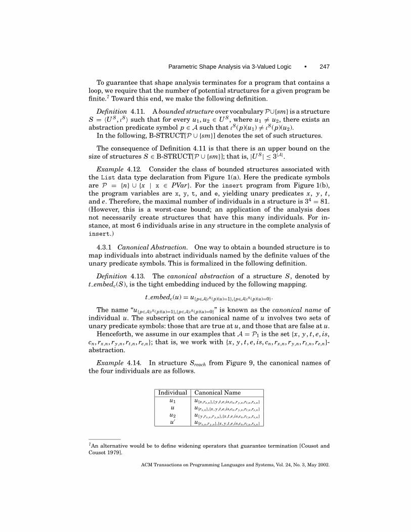
The name “u{p∈A|ιS (p)(u)=1},{p∈A|ιS (p)(u)=0}” is known as the canonical name ofindividual u. The subscript on the canonical name of u involves two sets ofunary predicate symbols: those that are true at u, and those that are false at u.

Henceforth, we assume in our examples that A = P1 is the set {x, y , t, e, is,cn, rx,n, ry ,n, rt,n, re,n}; that is, we work with {x, y , t, e, is, cn, rx,n, ry ,n, rt,n, re,n}-abstraction.

Example 4.14. In structure Sreach from Figure 9, the canonical names ofthe four individuals are as follows.

Individual Canonical Nameu1 u{x,rx,n},{ y ,t,e,is,cn,ry ,n,rt,n,re,n}u u{rx,n},{x, y ,t,e,is,cn,ry ,n,rt,n,re,n}u2 u{ y ,rx,n,ry ,n},{x,t,e,is,cn,rt,n,re,n}u′ u{rx,n,ry ,n},{x, y ,t,e,is,cn,rt,n,re,n}

7An alternative would be to define widening operators that guarantee termination [Cousot andCousot 1979].



Note that t embedc can be applied to any 3-valued structure, not just 2-valuedstructures, and that t embedc is idempotent (i.e., t embedc(t embedc(S)) =t embedc(S)).

For any two bounded structures S, S′ ∈ B-STRUCT[P ∪ {sm}], it is possibleto check whether S is isomorphic to S′, in time linear in the (explicit) sizes ofS and S′, using the following two-phase procedure.

(1) Rename the individuals in U S and U S′ according to their canonical names.(2) For each predicate symbol p ∈ P ∪{sm}, check that the predicates ιS(p) and

ιS′(p) are equal.

4.3.2 Relationship of Canonical Abstraction to Previous Work. Canonicalabstraction is a generalization of the abstraction functions that have been usedin some of the previous work on shape analysis [Jones and Muchnick 1981;Chase et al. 1990; Wang 1994; Sagiv et al. 1998].8 For instance, the abstractionpredicates used in Sagiv et al. [1988] are the “pointed-to-by-variable-x” pred-icates and thus correspond to the instantiation of canonical abstraction dis-cussed in Example 4.14. Earlier, Jones and Muchnick [1981] proposed makingeven finer distinctions by keeping exact information on elements within a dis-tance k from a variable. In Wang [1994], in addition to “pointed-to-by-variable-x” predicates, there are predicates of the form “was-pointed-to-by-variable-x-at-program-point-p.”

Definition 4.13 generalizes these ideas to define a set of bounded structuresin terms of any fixed set of unary “abstraction properties” on individuals.

OBSERVATION 4.15 (Abstraction Principle). Individuals are partitioned intoequivalence classes according to their sets of unary abstraction-property values.Every structure S\ is then represented (conservatively) by a condensed structureS in which each individual of S represents an equivalence class of individualsfrom S\. This method of collapsing structures always yields bounded structures.

Compared to previous work, however, the present article uses canonical ab-straction in somewhat different ways.

—Because the concrete and abstract worlds are defined in terms of a single uni-fied concept of logical structures, it is possible to apply t embedc to abstract(3-valued) structures as well as to concrete (2-valued) ones.

—The present work is not so tightly tied to canonical abstractions. There isnothing special about a bounded structure that uses canonical names; when-ever necessary, canonical names can be recovered from the values of a struc-ture’s unary predicates.

—At various stages, we work with nonbounded structures, and return tobounded structures by applying t embedc (see Section 6). The EmbeddingTheorem ensures that the operations we apply to 3-valued structures aresafe, even when we are working with nonbounded structures.

8The shape-analysis algorithms presented in Jones and Muchnick [1981], Chase et al. [1990], Wang[1994], and Sagiv et al. [1998] are described in terms of various kinds of Storage Shape Graphs(SSGs), not bounded structures. Our comparison is couched in the terminology of the present article.



Table V. Examples of Instrumentation Predicates

Pred. Intended Meaning Purpose Ref.is(v) Do two or more fields of heap ele-

ments point to v?lists and trees [Chase et al. 1990],

[Sagiv et al. 1998]rx,n(v) Is v (transitively) reachable from

pointer variable x along n fields?separating disjointdata structures

[Sagiv et al. 1998]

rn(v) Is v reachable from some pointer vari-able along n fields (i.e., is v a non-garbage element)?

compile-time garbagecollection

cn(v) Is v on a directed cycle of n fields? reference counting [Jones and Muchnick1981]

c f .b(v) Does a field-f deref. from v, followedby a field-b deref., yield v?

doubly linked lists [Hendren et al. 1992],[Plevyak et al. 1993]

cb. f (v) Does a field-b deref. from v, followedby a field-f deref., yield v?

doubly linked lists [Hendren et al. 1992],[Plevyak et al. 1993]

5. INSTRUMENTATION PREDICATES

It is possible to improve the precision of the analysis by using an abstract do-main that makes finer distinctions among the concrete structures. As discussedin Section 2.6, the instrumentation principle is the main tool for achieving this;that is, the notion of which finer distinctions to make is defined using instru-mentation predicates, which record information derived from other predicates.9

Formally, we assume that the set of predicates P is partitioned into two dis-joint sets: the core predicates, denoted by C, and the instrumentation predicates,denoted by I. Furthermore, the meaning of every instrumentation predicate isdefined in terms of a formula over the core predicates.10

Example 5.1. Table V lists some examples of instrumentation predicates,and Table VI gives their defining formulae.

Instrumentation predicates can increase the precision of a program-analysisalgorithm in at least the following ways:

(1) The value stored for an instrumentation predicate in a given 3-valued struc-ture S may be more precise than that obtained by evaluating the instru-mentation predicate’s defining formula (Observation 2.8). For example, instructure Sacyclic from Figure 6, ιSacyclic(cn)(u) = 0 despite the fact that ϕcn

evaluates to 1/2 on u.(2) The set of concrete structures that a given 3-valued structure S represents

(as defined by Equation (12)) is, in general, decreased if we augment Swith additional instrumentation predicates that have definite values for atleast some combinations of individuals. For example, structure Sacyclic fromFigure 6 is structure S3 from Figure 5 augmented with instrumentationpredicate cn, for which cn(u1) = 0 and cn(u) = 0. Thus, Sacyclic cannot possibly

9In the literature on logic, these predicates are sometimes called derived predicates.10For the sake of abbreviation, it is sometimes convenient to allow an instrumentation predicate’sdefining formula to be defined in terms of other instrumentation predicates; however, such definingformulae should not be mutually recursive.



Table VI. Formulae for the Instrumentation PredicatesListed in Table V

ϕis(v) def= ∃v1, v2 : n(v1, v) ∧ n(v2, v) ∧ v1 6= v2 (13)

ϕrx,n (v) def= x(v) ∨ ∃v1 : x(v1) ∧ n+(v1, v) (14)

ϕrn (v) def= ∨x∈PVar (x(v) ∨ ∃v1 : x(v1) ∧ n+(v1, v)) (15)

ϕcn (v) def= n+(v, v) (16)

ϕc f .b (v) def= ∀v1 : f (v, v1)⇒ b(v1, v) (17)

ϕcb. f (v) def= ∀v1 : b(v, v1)⇒ f (v1, v) (18)

represent 2-valued structures with cyclic nodes; in contrast, among thestructures that S3 represents is the following concrete cyclic list:

x u1 u2 u3n n

n

(3) Unary instrumentation predicates that are used as abstraction predicatesrefine the set of bounded structures. For example, using the “is-shared”predicate is as an abstraction predicate leads to an algorithm that is moreprecise than the one given in Sagiv et al. [1998]. The latter does not distin-guish between shared and unshared individuals, and thus loses accuracyfor stores that contain a shared heap cell that is not directly pointed to bya program variable. Adopting is as an additional abstraction predicate im-proves the accuracy of shape analysis because concrete-store elements thatare shared and concrete-store elements that are not shared are representedby abstract individuals that have different canonical names.

It is important to note that the instrumentation predicates do not have tobe unary. Furthermore, not all of the unary instrumentation predicates neednecessarily be used as abstraction predicates.

Adding more unary instrumentation predicates and using them as abstrac-tion predicates increases the worst-case cost of the analysis, since the numberof individuals in bounded structures is proportional to 3|A|. However, our initialexperience indicates that the opposite happens in practice; by using the “right”unary instrumentation predicates, the cost of the analysis can be significantlydecreased (see Section 7.4).

5.1 Updating Instrumentation Predicates

Because each instrumentation predicate is defined by means of a formula overthe core predicates (cf. Table VI), for the concrete semantics there is no need tospecify formulae for updating the instrumentation predicates. However, for theabstract semantics, the Instrumentation Principle implies that it may be moreprecise for a statement transformer to update the values of the instrumen-tation predicates explicitly. In particular, this is often the case for an instru-mentation predicate’s value for a summary node.

In order to update the values of the instrumentation predicates based onthe stored values of the instrumentation predicates, as part of instantiating



Table VII. Predicate-Update Formulae for the Instrumentation Predicate is

st ϕstis

x->n = NULL ϕstis (v) def=

{is(v) ∧ ϕis[n 7→ ϕst

n ] if ∃v′ : x(v′) ∧ n(v′, v)is(v) otherwise

x->n = t

(assuming thatx->n == NULL)

ϕstis (v) def=

{is(v) ∨ ϕis[n 7→ ϕst

n ] if ∃v1 : t(v) ∧ n(v1, v)is(v) otherwise

x = malloc() ϕstis (v) def= is(v) ∧ ¬new(v)

the parametric framework, the designer of a shape analysis must provide, forevery predicate p ∈ I and statement st, a predicate-update formula ϕst

p thatidentifies the new value of p after st. It is always possible to define ϕst

p tobe the formula ϕp[c 7→ ϕst

c | c ∈ C] (i.e., the formula obtained from ϕp by replac-ing each occurrence of a predicate c ∈ C by ϕst

c ).This substitution captures thevalue for c after st has been executed. We refer to ϕp[c 7→ ϕst

c | c ∈ C] as the triv-ial update formula for predicate p, since it is equivalent to merely reevaluatingp’s defining formula in the structure obtained after st has been executed. Asdemonstrated in Section 2, reevaluation may yield many indefinite values, andhence the trivial update formula is often unsatisfactory. It is preferable, there-fore, to devise predicate-update formulae that minimize reevaluations of ϕp.

We now state the requirements on predicate-update formulae that the userof our framework needs to show in order to make sure that the analysis isconservative.

Definition 5.2. We say that a predicate-update formula for p maintains thecorrect instrumentation for statement st if, for all S\ ∈ 2-STRUCT[P] and all Z ,[[

ϕstP

]]S\

2 (Z ) = [[ϕp]][[st]](S\)2 (Z ). (19)

In the above definition, [[st]](S\) denotes a version of the operation defined inDefinitions 3.3 and 3.5 in which P is restricted to C. We make the assumptionthat the predicate-update formula for an instrumentation predicate is definedsolely in terms of core predicates. An instrumentation predicate’s formula canalways be put in this form by repeated substitution until only core predicatesremain.

Henceforth, we assume that for all the instrumentation predicates andall the statements, the predicate-update formulae maintain correct instrumen-tation. Note that the trivial update formulae do maintain correct instrumenta-tion; however, they may yield very imprecise answers when applied to 3-valuedstructures.

5.2 Updating Sharing

Table VII gives the predicate-update formulae for the instrumentation predi-cate is. (It lists formulae only for the statements that may affect the value ofis.) The assignment to x->n = NULL can only change the value of is to 0, andonly for an element pointed to by x->n. Therefore, in Table VII ϕis[n 7→ ϕst

n ]is evaluated only for elements pointed to by x->n. Similarly, the assignmentx->n = t (assuming that x->n == NULL) can only change the value of is to 1,



Table VIII. Predicate-Update Formulae for Instrumentation Predicate rz,n, for ProgramsUsing the List Data Type Declaration from Figure 1(a)

st cond. ϕstrz,n

(v)

x = NULL z ≡ x 0z 6≡ x rz,n(v)

x = t z ≡ x rt,n(v)z 6≡ x rz,n(v)

x = t->n z ≡ x rt,n(v) ∧ (cn(v) ∨ ¬t(v))z 6≡ x rz,n(v)

x->n = NULL z ≡ x x(v)

z 6≡ x{ϕrz,n [n 7→ ϕst

n ] if cn(v) ∧ rx,n(v)rz,n(v) ∧ ¬(∃v′ : rz,n(v′) ∧ x(v′) ∧ rx,n(v) ∧ ¬x(v)) otherwise

x->n = t

(assuming that rz,n(v) ∨ (∃v′ : rz,n(v′) ∧ x(v′) ∧ rt,n(v))x->n == NULL)x = malloc() z ≡ x new(v)

z 6≡ x rz,n(v) ∧ ¬new(v)

Table IX. Predicate-Update Formulae forInstrumentation Predicate cn, for Programs Usingthe List Data Type Declaration from Figure 1(a)

st ϕstcn

(v)

x = NULL cn(v)x = t cn(v)x = t->n cn(v)x->n = NULL cn(v) ∧ ¬(∃v′ : x(v′) ∧ cn(v′) ∧ rx,n(v))x->n = t

(assuming that cn(v) ∨ ∃v′ : x(v′) ∧ rt,n(v′) ∧ rt,n(v)x->n == NULL)x = malloc() cn(v) ∧ ¬new(v)

and only for an element that is pointed to by t and already has at least oneincoming edge. Therefore, ϕis[n 7→ ϕst

n ] is evaluated only for elements that arepointed to by t and already have at least one incoming edge.

5.3 Updating Reachability and Cyclicity

In this section, we discuss how to define predicate-update formulae ϕstrx,n

(v) thatmaintain the correct instrumentation for the rx,n predicates. First, note that in a3-valued structure S, ϕrx,n(v) is likely to evaluate to 0 or 1/2 for most individuals:for [[ϕrx,n]]S

3 ([v 7→ u]) to evaluate to 1, there would have to be a path of n-edgesthat all have the value 1, from the individual pointed to by x to u. However,the Instrumentation Principle comes into play. As we show below, in manycases, by maintaining information about cyclicity in addition to reachability,information about the absence of a cycle can be used to update rx,n directly,without reevaluating ϕrx,n(v).

For programs that use the List data type declaration from Figure 1(a),predicate-update formulae for rx,n(v) and cn(v), are given in Tables VIII andIX, respectively. Some of these formulae update the value of rx,n(v) in terms of



Fig. 12. For the statement x->n = NULL, the above graph illustrates the chief obstacle for updat-ing reachability information. After execution of x->n = NULL, elements u4 and u5 are no longerreachable from z, whereas u2 (and u3) are still reachable from z. Note that beforehand the valueof rz,n is the same for u2, u4, and u5. For such individuals, Table VIII obtains the value of rz,n (inthe new structure) by evaluating the formula ϕrz,n [n 7→ ϕst

n ] (in the above structure).

the value of cn(v), and vice versa. For example, the predicate-update formulain the x->n = NULL case in Table VIII, when z 6≡ x, is based on the observa-tion that it is unnecessary to reevaluate ϕrz,n(v) whenever v does not occur on adirected cycle or is not reachable from x.

Let us now consider the predicate-update formulae for rx,n(v) that appear inTable VIII.

—The statement x = NULL resets rx,n to 0.—The statement x = t sets rx,n to rt,n.—The statement x = t->n sets rx,n for all individuals for which rt,n holds, except

for the individual u pointed to by t, unless u appears on a cycle, in which caserx,n(u) also holds.

—The statement x->n = NULL not only resets the x-reachability property rx,n,it may also change rz,n when the element directly pointed to by x is reachedby variable z. Furthermore, as illustrated in Figure 12, in the presence ofcycles it is not always obvious how to determine the exact elements whoserz,n properties change. Therefore, the predicate-update formula breaks intotwo subcases.—v appears on a directed cycle and is reachable from the individual pointed

to by x. In this case, ϕrz,n(v) is reevaluated (in the structure after thedestructive update). For 3-valued structures, this may lead to a loss ofprecision.

—v does not appear on a directed cycle or is not reachable from the individualpointed to by x. In this case, v fails to be reachable from z only if the edgebeing removed is used on the path from z to v.

—After the statement x = malloc(), the only element reachable from x is thenewly allocated element.

Let us now examine the predicate-update formulae for cn(v) that appear inTable IX.

—The statements x = NULL, x = t, and x = t->n do not change the n-predicates, and thus have no effect on cyclicity.

—If v′, the node pointed to by x, appears on a cycle, then the statementx->n = NULL breaks the cycle involving all the nodes reachable from x. (Thelatter cycle is unique, if it exists.) If the node pointed to by x does not appearon a cycle, this statement has no effect on cyclicity.



—If the node pointed to by x is reachable from t, then the statement x->n = tcreates a cycle involving all the nodes reachable from t. In other cases, nonew cycles are created.

—The statement x = malloc() sets the cyclicity property of the newly allocatedelement to 0.

6. ABSTRACT SEMANTICS

In this section, we formulate the abstract semantics for the shape-analysisframework. As an intermediate step, Section 6.1 first describes a simple ab-stract semantics based on the Reinterpretation Principle (Observation 2.9).This version shows how the machinery developed thus far fits together, butserves mainly as a strawman: this first approach yields very imprecise infor-mation about programs that perform list traversals and destructive updates(such as insert), and this failing motivates the development of two new piecesof machinery (focus and coerce) to refine the strawman approach. The mainideas behind the more refined approach are sketched in Section 6.2, and for-mally defined in Sections 6.3 and 6.4. Finally, Section 6.5 defines the more re-fined semantics, and also illustrates how it is capable of obtaining very preciseshape-analysis information when applied to the analysis of insert.

6.1 A Strawman Shape-Analysis Algorithm

We now define a simple abstract semantics for the shape-analysis frame-work based on the Reinterpretation Principle (Observation 2.9). The goal isto associate with each vertex v of control-flow graph G, a finite set of 3-valued structures StructSet[v] that “describes” all of the 2-valued structures inConcStructSet[v] (and possibly more). The abstract semantics can be expressedas the least fixed point (in terms of set inclusion) of the following system ofequations over the variables StructSet[v].

StructSet[v] =

{〈∅, ∅〉} if v = start⋃w→v∈E(G),w∈As(G)

{t embedc([[st(w)]]3(S)) | S ∈ StructSet[w]}

∪⋃

w→v∈E(G),w ∈ Id (G)

{S | S ∈ StructSet[w]}

∪⋃

w→v∈Tb(G)

{S | S ∈ StructSet[w] and S |=3 cond(w)}

∪⋃

w→v∈Fb(G)

{S | S ∈ StructSet[w] and S |=3 ¬cond(w)}

otherwise. (20)

This equation system closely resembles equation system (4), but has the follow-ing differences.



—The notation [[st(w)]]3 denotes the abstract meaning function for state-ment w; it is identical to the operation [[st(w)]] defined in Definitions 3.3and 3.5, except that the predicate-update formulae are evaluated in 3-valuedlogic.

—Instead of working with concrete 2-valued structures, equation system (20)operates on bounded structures and applies t embedc after every statement.

—When a formula cond(w) evaluates to 1/2, equation system (20) conserva-tively propagates information along both the true and the false branches.

The shape-analysis algorithm takes the form of an iterative procedure thatfinds the least fixed point of equation system (20). The iteration starts from theinitial assignment StructSet[v] = ∅ for each control-flow-graph vertex v. Be-cause of the t embedc operation, it is possible to check efficiently if two 3-valuedstructures are isomorphic.

Termination and safety of the shape-analysis algorithm are argued in thestandard manner [Cousot and Cousot 1977]. The algorithm terminates because,for any instantiation of the analysis framework, the set of bounded structuresis finite, and hence of finite height. Termination is assured because equationsystem (20) is monotonic (with respect to set inclusion).

The heart of the safety argument involves showing that the abstract trans-former that is applied along each edge of the control-flow graph is conservativewith respect to the corresponding transformer of the concrete semantics.

THEOREM 6.1 (Local Safety Theorem). If vertex w is a condition, then for allS ∈ 3-STRUCT[P ∪ {sm}]

(i) If S\ ∈ γ (S) and S\ |= cond(w), then S |=3 cond(w).(ii) If S\ ∈ γ (S) and S\ |= ¬cond(w), then S |=3 ¬cond(w).

If vertex w is a statement, then

(iii) If S\ ∈ γ (S), then [[st(w)]](S\) ∈ γ (t embedc([[st(w)]]3(S))).

PROOF. By Definition 4.8, S\ ∈ γ (S) means that there is a mapping f suchthat S\ v f S. Thus, properties (i) and (ii) follow immediately from the Embed-ding Theorem.

If vertex w is a statement, then it follows from the Embedding Theorem andthe definitions of [[st(w)]] and [[st(w)]]3 (Definitions 3.3 and 3.5) that, for anystructure S,

—If S\ ∈ γ (S), then [[st(w)]](S\) ∈ γ ([[st(w)]]3(S)).

In particular, this means that there is a mapping f such that [[st(w)]](S\) v f

[[st(w)]]3(S). However, t embedc simply folds together and renames individu-als from [[st(w)]]3(S), so we know that the composed mapping (t embedc ◦ f )embeds [[st(w)]](S\) into t embedc([[st(w)]]3(S)):

[[st(w)]](S\) v(t embedc ◦ f ) t embedc([[st(w)]]3(S)).

By the definition of γ (Definition 4.8), this implies property (iii). h



Fig. 13. An application of the strawman abstract transformer [[st0]]3 for statement st0: y = y->n

in insert.

THEOREM 6.2 (Global Safety Theorem). Let ConcStructSet[·] and Struct-Set[·] be the least-fixed-point solutions of equation systems (4) and (20), respec-tively. Then, for each vertex v of the control-flow graph,

ConcStructSet[v] ⊆⋃

S∈StructSet[v]

γ (S).

PROOF. Immediate from monotonicity and Theorem 6.1 (Local Safety), usingTheorem T2 of Cousot and Cousot [1977, p. 252]. h

Other variations on equation system (20) are possible. In particular, thefunction t embedc need not be applied after every statement; instead, it couldbe applied (i) at every merge point in the control-flow graph, or (ii) only inloops (e.g., at the target of each backedge in the control-flow graph). It is alsopossible to define a Hoare ordering on sets of structures that is induced by theembedding order.

Definition 6.3. For sets of structures XS1, XS1 ⊆ 3-STRUCT[P], XS1 vXS2 if and only if ∀S1 ∈ XS1 : ∃S2 ∈ XS2 : S1 v S2.

In principle, this could be used to remove nonmaximal structures during thecourse of the analysis; the shape-analysis algorithm would then be an iterativeprocedure to compute a least fixed point with respect to the Hoare order. How-ever, this would require being able to test the property S1 v S2 (i.e., whetherthere exists a function f that embeds S1 into S2).

Unfortunately, the use of the Reinterpretation Principle alone leads to shape-analysis algorithms that return very imprecise information. Figure 13 showsthe result of applying [[st0]]3 to structure Sa, one of the 3-valued structuresthat arises in the analysis of insert just before y is advanced down the listby the statement st0 : y = y->n. Similar to what was illustrated in Figure 10,the structure Sb that results is not as precise as what the abstract domainof canonical abstractions is capable of representing: for instance, Sb does notcontain a node that is definitely pointed to by y.

This imprecision leads to problems when a destructive update is performed.In particular, the first column in Table X shows what happens when the abstract



Table X.Selective applications of the abstract transformers using the strawman and refined approaches,for statements in insert that come after the search loop (for brevity, rz is used in place of rz,n forall variables z, and node names are not shown).



Fig. 14. One-stage vs. multistage abstract semantics for statement st0 : y = y->n. The focus andthe coerce operations are introduced in Sections 6.3 and 6.4, respectively. (This example is discussedin further detail in Sections 6.3 and 6.4.)

transformers for the five statements that follow the search loop in insert areapplied to Sb: Because y(v) evaluates to 1/2 for the summary node, we even-tually reach the situation shown in the fifth row of structures, in which y , e,rx , ry , re, rt , and is are all 1/2 for the summary node. As a result, under thestrawman approach, the abstract transformer for y->n = t sets the value ofcn for the summary node to 1/2. Consequently, the strawman analysis fails todetermine that the structure returned by insert is an acyclic list.

In contrast, the refined analysis described in the following subsections is ableto determine that at the end of insert the following properties always hold: (i)x points to an acyclic list that has no shared elements, (ii) y points into the tailof the x-list, and (iii) the values of e and y->n are equal.

It is worthwhile to note that the precision problem becomes even more acutefor shape-analysis algorithms that, like Chase et al. [1990], do not explicitlytrack reachability properties. The reason is that, without reachability, Sb rep-resents situations in which y points to an element that is not even part of thex-list.

6.2 An Overview of a More Precise Abstract Semantics

In formulating an improved approach, our goal is to retain an important prop-erty of the strawman approach, namely, that the transformer for a programstatement falls out automatically from the predicate-update formulae of theconcrete semantics and the predicate-update formulae supplied for the in-strumentation predicates. Thus, the main idea behind the more refined ap-proach is to decompose the transformer for st into a composition of sev-eral functions, as depicted in Figure 14 and explained below, each of whichfalls out automatically from the predicate-update formulae of the concrete se-mantics and the predicate-update formulae supplied for the instrumentationpredicates.

(1) The operation focus, defined in Section 6.3, refines 3-valued structures sothat the formulae that define the meaning of st evaluate to definite values.The focus operation thus brings these formulae “into focus.”

(2) The simple abstract meaning function for statement st, [[st]]3, is thenapplied.

(3) The operation coerce, defined in Section 6.4, converts a 3-valued struc-ture into a more precise 3-valued structure by removing certain kinds ofinconsistencies.



It is worthwhile noting that both focus and coerce are semantic-reductionoperations (a concept originally introduced in Cousot and Cousot [1979]). Thatis, they convert a set of 3-valued structures into a more precise set of 3-valuedstructures that describe the same set of stores. This property, together withthe correctness of the structure transformer [[st]]3, guarantees that the over-all multistage semantics is correct. In the context of a parametric frameworkfor abstract interpretation, semantic reductions are valuable because they al-low the transformers of the abstract semantics to be defined in a modularfashion.

It is also interesting to compare this approach to the best abstract trans-former defined in Cousot and Cousot [1979], which is obtained by applying theconcrete transformer to every concrete store that the input 3-valued structureS represents (i.e., to all of the 2-valued structures in γ (S)). The best abstracttransformer is conceptually simpler and potentially more precise, but cannotbe directly computed (since γ (S) is potentially infinite). In contrast, focus yieldsa finite set of 3-valued structures that represent the same concrete stores as S,and thus serves as a “partial concretization function.” Since [[st]]3 is conservativeby the Embedding Theorem, the overall result is guaranteed to be conserva-tive. Our experience has been that having focus ensure that the “important”formulae have definite values is sufficient to ensure that the overall result isprecise enough.

In contrast to focus, coerce does not depend on the particular statement st;it can be applied at any step, and may improve the precision of the analysis.In practice, it is often beneficial to also perform an application of coerce justafter the application of focus and before [[st]]3, so that the order of operationsbecomes focus, coerce, [[st]]3, coerce—followed by t embedc.

6.3 Bringing Formulae into Focus

In this section, we define an operation, called focus, that generates a set ofstructures on which a given set of formulae F have definite values for all as-signments. Unfortunately, in general focus may yield an infinite set of struc-tures. Therefore, in Section 6.3.1, we give a declarative specification of thedesired properties of the focus operation, and in Section 6.3.2, we give an al-gorithm that implements focus for a certain specific class of formulae that areneeded for shape analysis. The latter algorithm always yields a finite set ofstructures.

6.3.1 The Focus Operation. We extend operations on structures to opera-tions on sets of structures in the natural way. For an operation op that returnsa set (such as γ , [[st]]3, etc.),

op(XS) def=⋃

S∈XS

op(S). (21)

Definition 6.4. Given a set of formulae F , a function op : 3-STRUCT[P]→23-STRUCT[P] is a focus operation for F if for every S ∈ 3-STRUCT[P], op(S)



satisfies the following requirements.

—op(S) and S represent the same concrete structures; that is, γ (S) = γ (op(S))—In each of the structures in op(S), every formula ϕ ∈ F has a definite value

for every assignment; that is, for every S′ ∈ op(S), ϕ ∈ F , and assignmentZ , we have [[ϕ]]S′

3 (Z ) 6= 1/2.

In the above definition, Z maps the free variables of a formula ϕ ∈ F toindividuals in structures S′ ∈ op(S). In particular, when ϕ has one designatedfree variable v, Z maps v to an individual. As usual, when ϕ is a closed formula,the quantification over Z is superfluous.

Henceforth, we use the notation focusF , or simply focus when F is clear fromthe context, when referring to a focus operation for F in the generic sense. Weconsider a specific algorithm for focusing shortly.

The first obstacle to developing a general algorithm for focusing is that thenumber of resulting structures may be infinite. In many cases (including theones used below for shape analysis), this can be overcome by only generatingstructures that are maximal (in terms of the embedding order). However, insome cases the set of maximal structures is infinite, as well. This phenomenonis illustrated by the following example:

Example 6.5. Consider the following formula

ϕlast(v) def= ∀v1 : ¬n(v, v1),

which is true for the last heap cell of an acyclic singly linked list. Focusing onϕlast with the structure Sacyclic shown in Figure 6 will lead to an infinite set ofmaximal structures (lists of length 1, 2, 3, etc.).

To sidestep this obstacle, the focus formulae ϕ used in shape analysis aredetermined by the left-hand side L-values and right-hand side R-values of eachkind of statement in the programming language. These are formally defined inSection 6.3.2 and illustrated in the following example.

Example 6.6. For the statement st0: y = y->n in procedure insert, we focuson the formula

ϕ0(v) def= ∃v1 : y(v1) ∧ n(v1, v), (22)

which corresponds to the right-hand side R-value of st0 (the heap cell pointed toby y->n). The upper part of Figure 15 illustrates the application of focus{ϕ0}(Sa),where Sa is the structure shown in Figure 13 that occurs in insert just beforethe first application of statement st0: y = y->n. This results in three structures:Sa, f ,0, Sa, f ,1, and Sa, f ,2.

—In Sa, f ,0, [[ϕ0]]Sa, f ,0

3 ([v 7→ u]) equals 0. This structure represents a situationin which the concrete list that x and y point to has only one element, butthe store also contains garbage cells, represented by summary node u. (Aswe show later, this structure is actually inconsistent because of the valuesof the rx,n and ry ,n instrumentation predicates, and will be eliminated fromconsideration by coerce.)



Fig. 15. The first application of the improved transformer for statement st0: y = y->n in insert.

—In Sa, f ,1, [[ϕ0]]Sa, f ,1

3 ([v 7→ u]) equals 1. This covers the case where the list thatx and y point to has exactly two elements. For all of the concrete cells thatsummary node u represents, ϕ0 must evaluate to 1, and so u must representjust a single list node.

—In Sa, f ,2, [[ϕ0]]Sa, f ,2

3 ([v 7→ u.0]) equals 0 and [[ϕ0]]Sa, f ,2

3 ([v 7→ u.1]) equals 1. Thiscovers the case where the list that x and y point to is a list of three or moreelements. For all of the concrete cells that u.0 represents, ϕ0 must evaluateto 0, and for all of the cells that u.1 represents, ϕ0 must evaluate to 1. Thiscase captures the essence of node materialization as described in Sagiv et al.[1998]: individual u is bifurcated into two individuals.

Notice how focus{ϕ0}(Sa) can be effectively constructed from Sa by consider-ing the reasons why [[ϕ0]]Sa

3 (Z ) evaluates to 1/2 for various assignments Z . Insome cases, [[ϕ0]]Sa

3 (Z ) already has a definite value; for instance [[ϕ0]]Sa3 ([v 7→ u1])

equals 0, and therefore ϕ0 is already in focus at u1. In contrast, [[ϕ0]]Sa3 ([v 7→ u])

equals 1/2. There are three (maximal) structures S that we can construct fromSa in which [[ϕ0]]S

3 ([v 7→ u]) has a definite value:

— Sa, f ,0, in which ιSa, f ,0 (n)(u1, u) is set to 0, and thus [[ϕ0]]Sa, f ,0

3 ([v 7→ u]) equals 0;— Sa, f ,1, in which ιSa, f ,1 (n)(u1, u) is set to 1, and thus [[ϕ0]]Sa, f ,1

3 ([v 7→ u]) equals 1;



Table XI. The Target Formulae for Focus, for Statementsand Conditions of a Program that Uses Type List

st Focus Formulae

x = NULL ∅x = t {t(v)}x = t->n {∃v1 : t(v1) ∧ n(v1, v)}x->n = t {x(v), t(v)}x = malloc() ∅x == NULL {x(v)}x != NULL {x(v)}x == t {x(v), t(v)}x != t {x(v), t(v)}UninterpretedCondition ∅

— Sa, f ,2, in which u has been bifurcated into two different individuals, u.0and u.1. In Sa, f ,2, ιSa, f ,2 (n)(u1, u.0) is set to 0, and thus [[ϕ0]]Sa, f ,2

3 ([v 7→ u.0])equals 0, whereas ιSa, f ,2 (n)(u1, u.1) is set to 1, and thus [[ϕ0]]Sa, f ,2

3 ([v 7→u.1])equals 1.

Of course, there are other structures that can be embedded into Sa that wouldassign a definite value to ϕ0, but these are not maximal because each of themcan be embedded into one of Sa, f ,0, Sa, f ,1, or Sa, f ,2.

6.3.2 Selecting the Set of Focus Formulae for Shape Analysis. The greaterthe number of formulae on which we focus, the greater the number of dis-tinctions that the shape-analysis algorithm can make, leading to improvedprecision. However, using a larger number of focus formulae can increase thenumber of structures that arise, thereby increasing the cost of analysis. Ourpreliminary experience indicates that in shape analysis there is a simple wayto define the formulae on which to focus that guarantees that the number ofstructures generated grows only by a constant factor. The main idea is that ina statement of the form lhs = rhs, we only focus on formulae that define theheap cells for the L-value of lhs and the R-value of rhs. Focusing on left-handside L-values and right-hand side R-values ensures that the application of theabstract transformer does not set to 1/2 the entries of core predicates thatcorrespond to pointer variables and fields that are updated by the statement.This approach extends naturally to program conditions and to statements thatmanipulate multiple left-hand side L-values and right-hand side R-values.

For our simplified language and type List, the target formulae on which tofocus can be defined as shown in Table XI. Let us examine a few of the casesfrom Table XI.

—For the statement x = NULL, the set of target formulae is the empty set be-cause neither the left-hand side L-value nor the right-hand side R-value is aheap cell.

—For the statement x = t->n, the set of target formulae is the singleton set{∃v1 : t(v1) ∧ n(v1, v)} because the left-hand side L-value cannot be a heapcell, and the right-hand side R-value is the cell pointed to by t->n.



—For the statement x->n = t, the set of target formulae is the set {x(v), t(v)}because the left-hand side L-value is the heap cell pointed to by x and theright-hand side R-value is the heap cell pointed to by t.

—For the condition x == t, the set of target formulae is the set {x(v), t(v)}; theR-values of the two sides of the conditional expression are the heap cellspointed to by x and t.

It is not hard to extend Table XI for statements that manipulate more com-plicated data structures involving chains of selectors. For example, the set oftarget formulae for the statement x->a->b = y->c->d->e is

{∃v1 : x(v1) ∧ a(v1, v), ∃v1, v2, v3 : y(v1) ∧ c(v1, v2) ∧ d (v2, v3) ∧ e(v3, v)},because the left-hand side L-value is the heap cell pointed to by x->a, and theright-hand side R-value is the heap cell pointed to by y->c->d->e.

Figure 16 contains an algorithm that implements focus for the type of for-mulae that arise in Table XI.11 Here we observe that for every set of formulaeF1∪ F2, it is possible to focus on F1∪ F2 by first focusing on F1, and then on F2.Thus, it is sufficient to provide an algorithm that focuses on an individual for-mula ϕ. As shown in Table XI, in shape analysis there are two types of formulaethat must be considered:

—ϕ ≡ x(v), for x ∈ PVar. In this case, FocusVar(S, x) is applied;—ϕ ≡ ∃v1 : x(v1) ∧ n(v1, v), for x ∈ PVar. In this case, FocusVarDeref(S, x, n) is

applied.

FocusVar repeatedly eliminates more and more indefinite values for x(v) bycreating more and more structures. For every individual u for which ιS(x)(u)is an indefinite value, two or three structures are created. The function Ex-pand creates a structure in which individual u is bifurcated into two individ-uals; this captures the essence of shape-node materialization (cf. Sagiv et al.[1998]).

FocusVarDeref first brings x(v) into focus (by invoking FocusVar), and thenproceeds to eliminate indefinite ιS(n) values.

Example 6.7. Consider the application of FocusVarDeref(Sa, y, n) for struc-ture Sa from Figure 15. In this case, FocusVar(Sa, y) = {Sa}. When Sa is selectedfrom WorkSet, structures Sa, f ,0, Sa, f ,1, and Sa, f ,2 are created. In the next threeiterations, these structures are moved to AnswerSet.

The following two lemmas guarantee that the algorithm for focus shown inFigure 16 is correct.

LEMMA 6.8. For ϕ ≡ x(v), and for every structure S ∈ 3-STRUCT[P],FocusVar(S, y) is a focus operation for {ϕ}.

11An enhanced focus algorithm, which generalizes the methods describe here, is described inLev-Ami [2000]. This algorithm can be applied to an arbitrary formula, but may not always succeed.



Fig. 16. An algorithm for focus for the two types of formulae that arise in Table XI.

LEMMA 6.9. For ϕ ≡ ∃v1 : x(v1) ∧ n(v1, v), and for every structure S ∈3-STRUCT[P], FocusVarDeref(S, y, n) is a focus operation for {ϕ}.

It is not hard to see that both FocusVar and FocusVarDeref always return afinite (although not necessarily maximal) set of structures.

We use Focus to denote the operation that invokes FocusVar orFocusVarDeref, as appropriate.



6.4 Coercing into More Precise Structures

In this section, we define the operation coerce, which converts a 3-valued struc-ture into a more precise 3-valued structure by removing certain kinds of incon-sistencies.

Example 6.10. After focus, the simple transformer [[st]]3 is applied to eachof the structures produced. In the example discussed in Examples 6.6 and 6.7,[[st0]]3 is applied to structures Sa, f ,0, Sa, f ,1, and Sa, f ,2 to obtain structures Sa,o,0,Sa,o,1, and Sa,o,2, respectively (see Figure 15).

However, this process can produce structures that are not as precise aswe would like. The intuitive reason for this state of affairs is that there canbe interdependences between different properties stored in a structure, andthese interdependences are not necessarily incorporated in the definitions ofthe predicate-update formulae. In particular, consider structure Sa,o,2. In thisstructure, the n field of u.0 can point to u.1, which suggests that y may bepointing to a heap-shared cell. However, this is incompatible with the fact thatι(is)(u.1) = 0—that is, u.1 cannot represent a heap-shared cell—and the factthat ι(n)(u1, u.1) = 1—that is, it is known that u.1 definitely has an incoming nedge from a cell other than u.0.

Also, the structure Sa,o,0 describes an impossible situation: ι(ry ,n)(u) = 1 andyet u is not reachable (or even potentially reachable) from a heap cell that ispointed to by y.

In this section, we develop a systematic way to capture interdependencesamong the properties stored in 3-valued structures. The mechanism that wepresent removes indefinite values that violate certain consistency rules, thereby“sharpening” the structures that arise during shape analysis. This allows usto remedy the imprecision illustrated in Example 6.10. In particular, when thesharpening process is applied to structure Sa,o,2 from Figure 15, the structurethat results is Sb,2. In this case, the sharpening process discovers that (i) twoof the n-edges with value 1/2 can be removed from Sa,o,2, and (ii) individualu.1 can only ever represent a single individual in each of the structures thatSa,o,2 represents, and hence u.1 should not be labeled as a summary node. Thesefacts are not something that the mechanisms that have been described in earliersections are capable of discovering. Also, the structure Sa,o,0 is discarded by thesharpening process.

The sharpening mechanism is crucial to the success of the improved shape-analysis framework because it allows a more accurate job of materializationto be performed than would otherwise be possible. For instance, note how thesharpened structure, Sb,2, clearly represents an unshared list of length 3 ormore that is pointed to by x and whose second element is pointed to by y. Infact, in the abstract domain of canonical abstractions that is being used inour examples, Sb,2 is the most precise representation possible for the family ofunshared lists of length 3 or more that are pointed to by x and whose secondelement is pointed to by y. Without the sharpening mechanism, instantiationsof the framework would rarely be able to determine such things as “The data



structure being manipulated by a certain list-manipulation program is actuallya list.”

This subsection is organized as follows: Section 6.4.1 discusses how struc-tures should obey certain consistency rules. Section 6.4.2 discusses how we canobtain a system of “compatibility constraints” that formalize such consistencyrules; the constraint system is obtained automatically from formulae that ex-press certain global invariants on concrete stores. Compatibility constraintsare used in Section 6.4.3 to define an operation, called coerce, that “coerces”a structure into a more precise structure. Finally, in Section 6.4.4, we give analgorithm for coerce.

6.4.1 Compatibility Constraints. We can, in many cases, sharpen some ofthe stored predicate values of 3-valued structures:

Example 6.11. Consider a 2-valued structure S\ that can be embedded in a3-valued structure S, and suppose that the formula ϕis for “inferring” whetheran individual u is shared evaluates to 1 in S (i.e., [[ϕis(v)]]S

3 ([v 7→ u]) = 1). Bythe Embedding Theorem (Theorem 4.9), ιS

\

(is)(u\) must be 1 for any individualu\ ∈ U S\

that the embedding function maps to u.Now consider a structure S′ that is equal to S except that ιS

′(is)(u) is 1/2.

S\ can also be embedded in S′. However, the embedding of S\ in S is a “better”embedding; it is a “tighter embedding” in the sense of Definition 4.6. This hasoperational significance: it is needlessly imprecise to work with structure S′

in which ιS′(is)(u) has the value 1/2; instead, we should discard S′ and work

with S. In general, the “stored predicate” is should be at least as precise as itsinferred value; consequently, if it happens that ϕis evaluates to a definite value(1 or 0) in a 3-valued structure, we can sharpen the stored predicate is.

Similar reasoning allows us to determine, in some cases, that a structureis inconsistent. In Sa,o,0, for instance, ϕry ,n(u) = 0, whereas ιSa,o,0 (ry ,n)(u) is 1;consequently, Sa,o,0 is a 3-valued structure that does not represent any con-crete structures at all! This structure can therefore be eliminated from furtherconsideration by the abstract-interpretation algorithm.

This reasoning applies to all instrumentation predicates, not just is and rx,n,and to both of the definite values, 0 and 1.

The reasoning used in Example 6.11 can be summarized as the followingprinciple.

OBSERVATION 6.12 (The Sharpening Principle). In any structure S, the valuestored for ιS(p)(u1, . . . , uk) should be at least as precise as the value of p’sdefining formula ϕp, evaluated at u1, . . . , uk (i.e., [[ϕp]]S

3 ([v1 7→ u1, . . . , vk 7→ uk])).Furthermore, if ιS(p)(u1, . . . , uk) has a definite value and ϕp evaluates to an in-comparable definite value, then S is a 3-valued structure that does not representany concrete structures at all.

This observation motivates the subject of the remainder of this subsec-tion: an investigation of compatibility constraints expressed in terms of a newconnective x .



Definition 6.13. A compatibility constraint is a term of the form ϕ1 x ϕ2,where ϕ1 is an arbitrary 3-valued formula, and ϕ2 is either an atomic formulaor the negation of an atomic formula over distinct logical variables.

We say that a 3-valued structure S and an assignment Z satisfy ϕ1 x ϕ2, de-noted by S, Z |= ϕ1 x ϕ2, if whenever Z is an assignment such that [[ϕ1]]S

3 (Z ) =1, we also have [[ϕ2]]S

3 (Z ) = 1. (Note that if [[ϕ1]]S3 (Z ) equals 0 or 1/2, S and Z

satisfy ϕ1 x ϕ2, regardless of the value of [[ϕ2]]S3 (Z ).)

We say that S satisfies ϕ1 x ϕ2, denoted by S |= ϕ1 x ϕ2, if for every Z wehave S, Z |= ϕ1 x ϕ2. If 6 is a finite set of compatibility constraints, we writeS |= 6 if S satisfies every constraint in 6.

The compatibility constraint that captures the reasoning used inExample 6.11 is ϕis(v) x is(v). That is, when ϕis evaluates to 1 at u, then ismust evaluate to 1 at u in order to satisfy the constraint. The compatibilityconstraint used to capture the similar case of sharpening ι(is)(u) from 1/2 to 0is ¬ϕis(v) x ¬is(v).

Section 6.4.4 presents a constraint-satisfaction algorithm that repeatedlysearches for assignments Z such that S, Z 6|= ϕ1 x ϕ2 (i.e., [[ϕ1]]S

3 (Z ) = 1, but[[ϕ2]]S

3 (Z ) 6= 1). This algorithm is used to improve the precision of shape analysisby (i) sharpening the values of predicates stored in S (when the constraintviolation is repairable), and (ii) eliminating S from further consideration whenthe constraint violation is irreparable.

6.4.2 From Formulae to Constraints. Compatibility constraints provide away to express certain properties that are a consequence of the tight-embeddingprocess, but that would not be expressible with formulae alone. For a 2-valuedstructure, x has the same meaning as implication. (That is, if S is a 2-valuedstructure, S, Z |= ϕ1 x ϕ2 if and only if S, Z |= ϕ1 ⇒ ϕ2.) However, for a3-valued structure, x is stronger than implication: if ϕ1 evaluates to 1 and ϕ2evaluates to 1/2, the constraint ϕ1 x ϕ2 is not satisfied. More precisely, supposethat [[ϕ1]]S

3 (Z )= 1 and [[ϕ2]]S3 (Z )= 1/2; the implication ϕ1⇒ϕ2 is satisfied (i.e.,

S, Z |= ϕ1⇒ϕ2), but the constraint ϕ1 x ϕ2 is not satisfied (i.e., S, Z 6|= ϕ1 x ϕ2).In general, compatibility constraints are not expressible in Kleene’s logic

(i.e., by means of a formula that simulates the connective x ). The reason is thatformulae are monotonic in the information order (see Lemma 4.4), whereas x isnonmonotonic in its right-hand side argument. For instance, the constraint1 x p is satisfied in the structure S = 〈∅, [p 7→ 1]〉; however, it is not satisfiedin S′ = 〈∅, [p 7→ 1/2]〉 w S.

Thus, in 3-valued logic, compatibility constraints are in some sense “better”than formulae. Fortunately, compatibility constraints can be generated auto-matically from formulae that express certain global invariants on concretestores. We call such formulae compatibility formulae. There are two sourcesof compatibility formulae:

—the formulae that define the instrumentation predicates; and—additional formulae (“hygiene conditions”) that formalize the properties of

stores that are compatible with the semantics of C (i.e., with our encoding ofC stores as 2-valued logical structures).



In the remainder of the article, 2-CSTRUCT[P, F ] denotes the set of compatible2-valued structures that satisfy a given set of compatibility formulae F .12

The following definition supplies a way to convert formulae into constraints.

Definition 6.14. Let ϕ be a closed formula, and (where applicable below)let a be an atomic formula such that (i) a contains no repetitions of logicalvariables, and (ii) a 6≡ sm(v). Then the constraint generated from ϕ, denoted byr(ϕ), is defined as follows.

r(ϕ) = ϕ1 x a if ϕ ≡ ∀v1, . . . vk : (ϕ1 ⇒ a) (23)r(ϕ) = ϕ1 x ¬a if ϕ ≡ ∀v1, . . . vk : (ϕ1 ⇒ ¬a) (24)r(ϕ) = ¬ϕ x 0 otherwise. (25)

For a set of formulae F , we define r(F ) to be the set of constraints generatedfrom the formulae in F (i.e., {r(ϕ) | ϕ ∈ F }).

The intuition behind (23) and (24) is that for an atomic predicate, a tightembedding yields 1/2 only in cases in which a evaluates to 1 on one tuple ofvalues for v1, . . . , vk , but evaluates to 0 on a different tuple of values. In this case,the left-hand side will evaluate to 1/2 as well (see Lemma 6.15 below). Rule (25)is included to enable an arbitrary formula to be converted to a constraint.

The following lemma guarantees that tight embedding preserves satisfactionof r(F ).

LEMMA 6.15. For every pair of structures S\ ∈ 2-CSTRUCT[P, F ] and S ∈3-STRUCT[P] such that S is a tight embedding of S\, S |= r(F ).

PROOF. See Appendix C. ¤

Example 6.16. It is worthwhile to point out that tight embedding need notpreserve implications when the right-hand side is an arbitrary formula. Inparticular, it does not hold for disjunctions. Consider the implication formula

∀v : 1⇒ p1(v) ∨ p2(v)

and the structure S\ = 〈{u1, u2}, ι\〉 with two individuals, u1 and u2, such that

ι\ = [sm 7→ [u1 7→ 0, u2 7→ 0], p1 7→ [u1 7→ 1, u2 7→ 0], p2 7→ [u1 7→ 0, u2 7→ 1]].

Let S be the tight embedding of S\ obtained by mapping both u1 and u2 intothe same individual u1,2; that is, S = 〈{u1,2}, ι〉), where

ι = [sm 7→ [u1,2 7→ 1/2], p1 7→ [u1,2 7→ 1/2], p2 7→ [u1,2 7→ 1/2]].

We see that S\ |= 1 ⇒ p1(v) ∨ p2(v) but S 6|= 1 x p1(v) ∨ p2(v) since[[p1(v) ∨ p2(v)]]S

3 ([v 7→ u1,2]) = 1/2, whereas [[1]]S3 ([v 7→ u1,2]) = 1.

12We also use a weaker notion of when a predicate-update formula for p maintains the correctinstrumentation for statement st; in particular, in Definition 5.2, the occurrence of 2-STRUCT[P]is replaced by 2-CSTRUCT[P, F ]. The notion of concretization (Definition 4.8) is adjusted in thesame manner.



Table XII.The set of formulae listed above the line are the compatibility formulae gen-erated for the instrumentation predicates is, cn, and rx,n. The correspondingcompatibility constraints are listed below the line.

∀v : (∃v1, v2 : n(v1, v) ∧ n(v2, v) ∧ v1 6= v2) ⇒ is(v) (27)∀v : ¬(∃v1, v2 : n(v1, v) ∧ n(v2, v) ∧ v1 6= v2) ⇒ ¬is(v) (28)

∀v : n+(v, v) ⇒ cn(v) (29)∀v : ¬n+(v, v) ⇒ ¬cn(v) (30)

for each x ∈ PVar, ∀v : x(v) ∨ ∃v1 : x(v1) ∧ n+(v1, v) ⇒ rx,n(v) (31)for each x ∈ PVar, ∀v : ¬(x(v) ∨ ∃v1 : x(v1) ∧ n+(v1, v)) ⇒ ¬rx,n(v) (32)

(∃v1, v2 : n(v1, v) ∧ n(v2, v) ∧ v1 6= v2) x is(v) (33)¬(∃v1, v2 : n(v1, v) ∧ n(v2, v) ∧ v1 6= v2) x ¬is(v) (34)

n+(v, v) x cn(v) (35)¬n+(v, v) x ¬cn(v) (36)

for each x ∈ PVar : x(v) ∨ ∃v1 : x(v1) ∧ n+(v1, v) x rx,n(v) (37)for each x ∈ PVar : ¬(x(v) ∨ ∃v1 : x(v1) ∧ n+(v1, v)) x ¬rx,n(v) (38)

Compatibility Constraints from Instrumentation Predicates. Our firstsource of compatibility formulae is the set of formulae that define the instru-mentation predicates. For every instrumentation predicate p ∈ I defined by aformula ϕp(v1, . . . , vk), we generate a compatibility formula of the form

∀v1, . . . , vk : ϕp(v1, . . . , vk)⇔ p(v1, . . . , vk). (26)

So that we can apply Definition 6.14, this is then broken into two implications:

∀v1, . . . , vk : ϕp(v1, . . . , vk) ⇒ p(v1, . . . , vk)∀v1, . . . , vk : ¬ϕp(v1, . . . , vk) ⇒ ¬p(v1, . . . , vk).

For instance, for the instrumentation predicate is, we use formula (13) for ϕisto generate compatibility formulae (27) and (28), which lead to compatibilityconstraints (33) and (34) (see Table XII).

Compatibility Constraints from Hygiene Conditions. Our second sourceof compatibility formulae stems from the fact that not all structures S\ ∈2-STRUCT[P] represent stores that are compatible with the semantics of C.For example, stores have the property that each pointer variable points to atmost one element in heap-allocated storage.

Example 6.17. The set of formulae FList, listed above the line in Table XIII,is a set of compatibility formulae that must be satisfied for a structure to repre-sent a store of a C program that operates on values of the type List defined inFigure 1(a). Formula (39) captures the condition that concrete stores never con-tain any summary nodes. Formula (40) captures the fact that every programvariable points to at most one list element. Formula (41) captures a similarproperty of the n fields of List structures: Whenever the n field of a list elementis non-NULL, it points to at most one list element. The corresponding compat-ibility constraints generated according to Definition 6.14 are listed below theline.

Compatibility Constraints from “Extended Horn Clauses.” The constraint-generation rules defined in Definition 6.14 generate interesting constraints



Table XIII.The set of formulae listed above the line, denoted by FList, are com-patibility formulae for structures that represent a store of a C pro-gram that operates on values of the type List defined in Figure 1(a).The corresponding compatibility constraints r(FList) are listed belowthe line.

¬∃v : sm(v) (39)for each x ∈ PVar, ∀v1, v2 : x(v1) ∧ x(v2) ⇒ v1 = v2 (40)

∀v1, v2 : (∃v3 : n(v3, v1) ∧ n(v3, v2)) ⇒ v1 = v2 (41)(∃v : sm(v)) x 0 (42)

for each x ∈ PVar, x(v1) ∧ x(v2) x v1 = v2 (43)(∃v3 : n(v3, v1) ∧ n(v3, v2)) x v1 = v2 (44)

only for certain specific syntactic forms, namely, implications with exactly one(possibly negated) predicate symbol on the right-hand side. Thus, when wegenerate compatibility constraints from compatibility formulae written as im-plications (cf. Tables XII and XIII), the set of constraints generated depends onthe form in which the compatibility formulae are written. In particular, not allof the many equivalent forms possible for a given compatibility formula leadto useful constraints. For instance, r(∀v1, . . . , vk : (ϕ ⇒ a)) yields the (useful)constraint ϕ x a, but r(∀v1, . . . , vk : (¬ϕ ∨ a)) yields the (not useful) constraint¬(¬ϕ ∨ a) x 0.

This phenomenon can prevent an instantiation of the shape-analysis frame-work from having a suitable compatibility constraint at its disposal that wouldotherwise allow it to sharpen or discard a structure that arises during theanalysis, and hence can lead to a shape-analysis algorithm that is more conser-vative than we would like. However, when compatibility formulae are writtenas “extended Horn clauses” (see Definition 6.18 below), the way around this dif-ficulty is to augment the constraint-generation process to generate constraintsfor some of the logical consequences of each compatibility formula. The processof “generating some of the logical consequences for extended Horn clauses” isformalized as follows.

Definition 6.18. For a formula ϕ, we define ϕ1 ≡ ϕ and ϕ0 ≡ ¬ϕ. We saythat a formula ϕ of the form

∀ . . . :m∨

i=1

(ϕi)Bi ,

where m > 1 and Bi ∈ {0, 1}, is an extended Horn clause. We define the closureof ϕ, denoted by closure(ϕ), to be the following set of formulae.

closure(ϕ) def=

∀ . . . , ∃v1, v2, . . . , vn :m∧

i=1,i 6= j

ϕ1−Bii ⇒ ϕ

Bjj

∣∣∣∣∣∣∣1 ≤ j ≤m,vk ∈ freeVars(ϕ),vk 6∈ freeVars(ϕ j )

. (45)

For a formula ϕ that is not an extended Horn clause, closure(ϕ) = {ϕ}. Finally,for a set of formulae F , we write closure(F ) to denote the application of closureto every formula in F .



Table XIV.

The compatibility formulae closure(FList) generated via Definition 6.18when the two implication formulae in FList, (40) and (41), are expressedas the extended Horn clauses (50) and (51), respectively (Note thatthe systematic application of Definition 6.18 leads, in this case, to twopairs of formulae that differ only in the names of their bound variables:(46)/(47) and (48)/(49).)

¬∃v : sm(v) (39)for each x ∈ PVar, ∀v1, v2 : x(v1) ∧ x(v2)⇒ v1 = v2 (40)

for each x ∈ PVar, ∀v2 : (∃v1 : x(v1) ∧ v1 6= v2)⇒ ¬x(v2) (46)for each x ∈ PVar, ∀v1 : (∃v2 : x(v2) ∧ v1 6= v2)⇒ ¬x(v1) (47)

∀v1, v2 : (∃v3 : n(v3, v1) ∧ n(v3, v2))⇒ v1 = v2 (41)∀v2, v3 : (∃v1 : n(v3, v1) ∧ v1 6= v2)⇒ ¬n(v3, v2) (48)∀v1, v3 : (∃v2 : n(v3, v2) ∧ v1 6= v2)⇒ ¬n(v3, v1) (49)

It is easy to see that the formulae in closure(ϕ) are implied by ϕ.

Example 6.19. The set of formulae listed in Table XIV are the compatibilityformulae closure(FList) generated via Definition 6.18 when the two implicationformulae in FList, (40) and (41), are expressed as the following extended Hornclauses (i.e., by rewriting the implications as disjunctions, and then applyingDe Morgan’s laws).

for each x ∈ PVar, ∀v1, v2 : ¬x(v1) ∨ ¬x(v2) ∨ v1 = v2. (50)∀v1, v2, v3 : ¬n(v3, v1) ∨ ¬n(v3, v2) ∨ v1 = v2. (51)

From (50) and (51), Definition 6.14 generates the final six compatibility formu-lae shown in Table XIV. By Definition 6.14 these yield the following compati-bility constraints.

for each x ∈ PVar, x(v1) ∧ x(v2) x v1 = v2 (43)for each x ∈ PVar, (∃v1 : x(v1) ∧ v1 6= v2) x ¬x(v2) (52)for each x ∈ PVar, (∃v2 : x(v2) ∧ v1 6= v2) x ¬x(v1) (53)

(∃v3 : n(v3, v1) ∧ n(v3, v2)) x v1 = v2 (44)(∃v1 : n(v3, v1) ∧ v1 6= v2) x ¬n(v3, v2) (54)(∃v2 : n(v3, v2) ∧ v1 6= v2) x ¬n(v3, v1). (55)

Similarly, after (27) is rewritten as the following extended Horn clause

∀v, v1, v2 : ¬n(v1, v) ∨ ¬n(v2, v) ∨ v1 = v2 ∨ is(v),

we obtain the following compatibility constraints.

(∃v1, v2 : n(v1, v) ∧ n(v2, v) ∧ v1 6= v2) x is(v) (33)(∃v1 : n(v1, v) ∧ v1 6= v2 ∧ ¬is(v)) x ¬n(v2, v) (56)(∃v2 : n(v2, v) ∧ v1 6= v2 ∧ ¬is(v)) x ¬n(v1, v) (57)(∃v : n(v1, v) ∧ n(v2, v) ∧ ¬is(v)) x v1 = v2. (58)



As we show in Section 6.4.4, the use of constraints—and, in particular, theones created from formulae generated by closure—plays a crucial role in theshape-analysis framework. In particular, constraint (56) (or the equivalent con-straint (57)) allows a more accurate job of materialization to be performed thanwould otherwise be possible: When is(u) is 0 and one incoming n edge to u is 1,to satisfy constraint (56) a second incoming n edge to u cannot have the value1/2; it must have the value 0. That is, the latter edge cannot exist (cf. Exam-ples 6.10 and 6.26). This allows edges to be removed (safely) that a more naivematerialization process would retain (cf. structures Sa,o,2 and Sb,2 in Figure 15),and permits the improved shape-analysis algorithm to generate more precisestructures for insert than the ones generated by the simple shape-analysisalgorithm described in Sections 2 and 6.1.

Henceforth, we assume that closure has been applied to all sets of compati-bility formulae.

Definition 6.20 (Compatible 3-Valued Structures). Given a set ofcompatibility formulae F , the set of compatible 3-valued structures3-CSTRUCT[P, r(F )] ⊆ 3-STRUCT[P] is defined by S ∈ 3-CSTRUCT[P, r(F )]if and only if S |= r(F ).

The following lemma ensures that we can always replace a struc-ture by a compatible one that satisfies constraint-set r(F ) without losinginformation.

LEMMA 6.21. For every structure S ∈ 3-STRUCT[P] and concrete structureS\ ∈ γ (S), there exists a structure S′ ∈ 3-CSTRUCT[P, (F )] such that (i) U S′ =U S , (ii) S′ v S, and (iii) S\ ∈ γ (S′).

PROOF. Let S\ ∈ γ (S), then by Definition 4.8 (as modified by footnote 12),S\ |= F and there exists a function f : U S\ → U S such that S\ v f S. DefineS′ = f (S\) (i.e., S′ is the tight embedding of S\ under f ). By Lemma 6.15, S′

satisfies the necessary requirements. h

In Section 6.4.4, we give an algorithm that constructs from S and r(F ) amaximal S′ meeting the conditions of Lemma 6.21 (without investigating thepossibly infinite set of actual concrete structures S\ ∈ γ (S)).

6.4.3 The Coerce Operation. We are now ready to show how the coerceoperation works.

Example 6.22. Consider structure Sa,o,2 from Figure 15. This structure vi-olates constraint (56) for the assignment [v 7→ u.1, v2 7→ u.0] when the vari-able v1 of the existential quantifier is bound to u1: because ι(n)(u1, u.1) = 1,u1 6= u.0, and ι(is)(u.1) = 0, but ι(n)(u.0, u.1) = 1/2, constraint (56) is not sat-isfied; the left-hand side evaluates to 1, whereas the right-hand side evaluatesto 1/2.

This example motivates the following definition.



Definition 6.23. The operation

coercer(F ) : 3-STRUCT[P]→ 3-CSTRUCT[P, r(F )] ∪ {⊥}is defined as follows: coercer(F )(S) def= the maximal S′ such that S′ v S, U S′ = U S ,and S′ ∈ 3-CSTRUCT[P, r(F )], or ⊥ if no such S′ exists.

(We simply write coerce when r(F ) is clear from the context.)It is a fact that the maximal such structure S′ is unique (if it exists), which

follows from the observation that compatible structures with the same universeof individuals are closed under the following join operation:

Definition 6.24. For every pair of structures S1, S2 ∈ 3-CSTRUCT[P, r(F )]such that U S1 = U S2 = U , the join of S1 and S2, denoted by S1 t S2, is definedas follows.

S1 t S2def= 〈U, λp.λu1, u2, . . . , um.ι

S1 (p)(u1, u2, . . . , um) t ιS2 (p)(u1, u2, . . . , um)〉.LEMMA 6.25. For every pair of structures S1, S2 ∈ 3-CSTRUCT[P, r(F )]

such that U S1 = U S2 = U, the structure S1 tS2 is also in 3-CSTRUCT[P, r(F )].

PROOF. See Appendix C. h

Because coerce can result in at most one structure, its definition does notinvolve a set former, in contrast to focus, which can return a nonsingleton set.The significance of this is that only focus can increase the number of structuresthat arise during shape analysis, whereas coerce cannot.

Example 6.26. The application of coerce to the structures Sa,o,0, Sa,o,1, andSa,o,2 yields Sb,1 and Sb,2, as shown in the bottom block of Figure 15.

—The structure Sa,o,0 is discarded because there exists no structure that canbe embedded into it that satisfies constraint (38).

—The structure Sb,1 was obtained from Sa,o,1 by removing incompatibilities asfollows:(1) Consider the assignment [v 7→ u, v1 7→ u1, v2 7→ u]. Because ι(n)(u1, u) =

1, u1 6= u, and ι(is)(u) = 0, constraint (56) implies that ι(n)(u, u) mustequal 0. Thus, in Sb,1 the (indefinite) n edge from u to u has been removed.

(2) Consider the assignment [v1 7→ u, v2 7→ u]. Because ι( y)(u) = 1, con-straint (43) implies that [[v1 = v2]]Sb,1

3 ([v1 7→ u, v2 7→ u]) must equal 1. ByDefinition 4.2, this means that ιSb,1 (sm)(u) must equal 0. Thus, in Sb,1 uis no longer a summary node.

—The structure Sb,2 was obtained from Sa,o,2 by removing incompatibilities asfollows:(1) Consider the assignment [v 7→ u.1, v1 7→ u1, v2 7→ u.0]. Because

ι(n)(u1, u.1) = 1, u1 6= u.0, and ι(is)(u.1) = 0, constraint (56) implies thatιSb,2 (n)(u.0, u.1) must equal 0. Thus, in Sb,2 the (indefinite) n edge fromu.0 to u.1 has been removed.

(2) Consider the assignment [v 7→ u.1, v1 7→ u1, v2 7→ u.1]. Becauseι(n)(u1, u.1) = 1, u1 6= u.1, and ι(is)(u.1) = 0, constraint (56) implies that



ιSb,2 (n)(u.1, u.1) must equal 0. Thus, in Sb,2 the (indefinite) n edge fromu.1 to u.1 has been removed.

(3) Consider the assignment [v1 7→ u.1, v2 7→ u.1]. Because ι( y)(u.1) = 1,constraint (43) implies that [[v1 = v2]]Sb,2

3 ([v1 7→ u.1, v2 7→ u.1]) must equal1. By Definition 4.2, this means that ιSb,2 (sm)(u.1) must equal 0. Thus, inSb,2 u.1 is no longer a summary node.

There are important differences between the structures Sb,1 and Sb,2 thatresult from applying the refined abstract transformer for statement st0 : y =y->n, compared with the structure Sb that results from applying the strawmanabstract transformer (see Figure 13). For instance, y points to a summary nodein Sb, whereas y does not point to a summary node in either Sb,1 or Sb,2; as notedearlier, in the abstract domain of canonical abstractions that is being used inour examples, Sb,2 is the most precise representation possible for the family ofunshared lists of length 3 or more that are pointed to by x and whose secondelement is pointed to by y.

6.4.4 The Coerce Algorithm. In this subsection, we describe an algorithm,called Coerce, that implements the operation coerce. This algorithm actuallyfinds a maximal solution to a system of constraints of the form defined inDefinition 6.13. It is convenient to partition these constraints into the followingtypes:

ϕ(v1, v2, . . . , vk) x 0 (59)ϕ(v1, v2, . . . , vk) x (v1 = v2)b (60)ϕ(v1, v2, . . . , vk) x pb(v1, v2, . . . , vk), (61)

where p 6= sm, and the superscript notation used is the same as in Defini-tion 6.18: ϕ1 ≡ ϕ and ϕ0 ≡ ¬ϕ. We say that constraints in the forms (59), (60),and (61) are Type I, Type II, and Type III constraints, respectively.

The Coerce algorithm is shown in Figure 17. The input is a 3-valued struc-ture S ∈ 3-STRUCT[P] and a set of constraints r(F ). It initializes S′ to theinput structure S and then repeatedly refines S′ by lowering predicate valuesin ιS

′from 1/2 to a definite value, until either: (i) a constraint is irreparably

violated (i.e., the left-hand and right-hand sides have different definite values,in which case the algorithm fails and returns⊥; or (ii) no constraint is violated,in which case the algorithm succeeds and returns S′. The main loop is a caseswitch on the type of the constraint considered.

—A violation of a Type I constraint is irreparable since the right-hand side isthe literal 0.

—A violation of a Type II constraint when the right-hand side is a negatedequality cannot be fixed. When v1 6= v2 does not evaluate to 1, we have Z (v1) =Z (v2); therefore, it is impossible to lower predicate values to force the formulav1 6= v2 to evaluate to 1 for assignment Z .

—A violation of a Type II constraint when the right-hand side is an equalitythat evaluates to 1/2 can be fixed. This type of violation occurs when there



Fig. 17. An iterative algorithm for solving 3-valued constraints.

is an individual u that is a summary node:

[[v1 = v2]]S′3 ([v1 7→ u, v2 7→ u]) = ιS′ (sm)(u) = 1/2.

In this case, ιS′(sm)(u) is set to 0.

—A violation of a Type III constraint can be fixed when the right-hand sidevalue is 1/2.

Example 6.27. When the Coerce algorithm is applied to Sa,o,0, the TypeIII constraint (38) for program variable y is irreparably violated, and ⊥ isreturned.

Coerce must terminate after at most n steps, where n is the number of definitevalues in S′, which is bounded by

∑p∈P |U |arity(p). Correctness is established by

the following theorem.

THEOREM 6.28. For every S ∈ 3-STRUCT[P], coercer(F )(S) = Coerce(S,r(F )).


6.5 The Shape-Analysis Algorithm

In this section, we define the more refined abstract semantics, which includesapplications of focus and coerce. (The actual algorithm uses Focus and Coerce.)The main idea is to refine equation system (20) by performing focus at thebeginning of each abstract transformer that is applied along an edge of the



control-flow graph, and coerce at the end. Formally, this is defined as follows.

StructSet[v] =

{〈∅, ∅〉} if v= start⋃w→v∈E(G),w∈As(G)

t embedc( coerce( [[st(w)]]3( focusF (w)(StructSet[w]))))

∪⋃

w→v∈E(G),w∈Id (G)

{S | S ∈ StructSet[w]}

∪⋃

w→v∈Tb(G)

{t embedc(S)

∣∣∣∣ S ∈ coerce( focusF (w)(StructSet[w]))and S |=3 cond(w)

}∪

⋃w→v∈Fb(G)

{t embedc(S)

∣∣∣∣ S ∈ coerce( focusF (w)(StructSet[w]))and S |=3 ¬cond(w)

}

otherwise.(62)

Here F (w) is the set of focus formulae for w (see Table XI).As with the strawman semantics, the safety argument involves showing that

the abstract transformer that is applied along each edge of the control-flowgraph is conservative with respect to the corresponding transformer of the con-crete semantics. Because focus and coerce are defined as semantic reductions,their presence in equation system (62) merely serves to increase the precisionof the final answer. As before, the safety of the uses of [[·]]3 and |=3 follow fromthe Embedding Theorem. Formally, we show the following local safety theorem:

THEOREM 6.29 (Local Safety Theorem). If vertex w is a condition, then forall S ∈ 3-STRUCT[P ∪ {sm}]

(i) If S\ ∈ γ (S) and S\ |= cond(w), then there exists S′ ∈ coerce(focusF (w)(S))such that S′ |=3 cond(w) and S\ ∈ γ (t embedc(S′)).

(ii) If S\ ∈ γ (S) and S\ |= ¬cond(w), then there exists S′ ∈ coerce(focusF (w)(S))such that S′ |=3 ¬cond(w) and S\ ∈ γ (t embedc(S′)).


(iii) If S\ ∈ γ (S), then [[st(w)]](S\) ∈ γ ( t embedc( coerce( [[st(w)]]3(focusF (w)(S))))).


The global safety property is argued in the same way as in the strawmansemantics.

Example 6.30. Table XV shows the 3-valued structures that occur beforeand after applications of the abstract transformer for the statement y = y->nduring the abstract interpretation of insert. (Because we are analyzing a singleprocedure, we allow an arbitrary set of 3-valued structures to hold at the entryof the procedure, as opposed to equation system (62), which assumes a single,empty initial structure. The global safety theorem still holds as long as all ofthe initial concrete structures are represented by the 3-valued structures thatare provided for the entry point.)



Table XV.The structures that occur before and after successive applications of the abstract transformerfor the statement y = y->n during abstract interpretation of insert (for brevity, node namesare not shown).



The material in Table X that appears under the heading “Refined Analysis”shows the application of the abstract transformers for the five statements thatfollow the search loop in insert to Sb,1 and Sb,2. For space reasons, we do notshow the abstract execution of these statements on the other structures shownin Table XV; however, the analysis is able to determine that at the end of insertthe following properties always hold: (i) x points to an acyclic list that has noshared elements, (ii) y points into the tail of the x-list, and (iii) the values of e andy->n are equal. The identification of the latter condition is rather remarkable:the analysis is capable of showing that e and y->n are must-aliases at the endof insert.

7. RELATED WORK

This article presents results from an effort to clarify and extend our previouswork on shape analysis [Sagiv et al. 1998]. Compared with Sagiv et al. [1998],the major differences are as follows.

—A single specific shape-analysis algorithm was presented in Sagiv et al.[1998]. The present article presents a parametric framework for shape anal-ysis. It provides the basis for generating different shape-analysis algorithmsby varying the instrumentation predicates used.

—This article uses different instantiations of the parametric framework toshow how shape analysis can be performed for a variety of different kinds oflinked data structures.

—The shape-analysis algorithm in Sagiv et al. [1998] was cast as an abstractinterpretation in which the abstract transfer functions transformed shapegraphs to shape graphs. The present work is based on logic, and shape graphsare replaced by 3-valued logical structures.

The use of logic has many advantages. The most important of these is that itrelieves the designer of a particular shape analysis from many of the burden-some tasks that the methodology of abstract interpretation ordinarily imposes.In particular, (i) the abstract semantics falls out automatically from the concretesemantics, and (ii) there is no need for a proof that a particular instantiationof the shape-analysis framework is correct: the soundness of all instantiationsof the framework follows from a single metatheorem, the Embedding Theorem,which shows that information extracted from a 3-valued structure is sound withrespect to information extracted from a corresponding 2-valued structure.

Of course, a trade-off is involved: with our approach it is necessary to de-fine the instrumentation predicates that are appropriate for a given analysis.It is also usually necessary to provide predicate-update formulae that specifyhow the values of instrumentation predicates are affected by the execution ofeach kind of statement in the programming language, and to prove that theseformulae maintain the correct instrumentation (in the sense of Definition 5.2and footnote 12). It is open to debate whether these are more or less burden-some tasks than those one faces with more standard approaches to abstractinterpretation.



A substantial amount of material covering previous work on pointer analysis,alias analysis, and shape analysis is presented in Sagiv et al. [1998]. In theremainder of this section, we confine ourselves to the work most relevant to thepresent article.

7.1 Previous Work on Shape Analysis

The following previous shape-analysis algorithms, which all make use of somekind of shape-graph formalism, can be viewed as instances of the frameworkpresented in this article.

—The algorithms of Wang [1994] and Sagiv et al. [1998] map unbounded-sizestores into bounded-size abstractions by collapsing concrete cells that are notdirectly pointed to by program variables into one abstract cell, whereas con-crete cells that are pointed to by different sets of variables are kept apart indifferent abstract cells. As discussed in Section 4.3, these algorithms are cap-tured in the framework by using abstraction predicates of the form pointed-to-by-variable-x (for all x ∈ PVar).

—The algorithm of Jones and Muchnick [1981], which collapses individualsthat are not reachable from a pointer variable in k or fewer steps, for somefixed k, can be captured in our framework by using instrumentation predi-cates of the form “reachable-from-x-via-access-path-α,” for |α| ≤ k.

—The algorithms of Jones and Muchnick [1982] and Chase et al. [1990] can becaptured in the framework by introducing unary core predicates that recordthe allocation sites of heap cells.

—The algorithm of Plevyak et al. [1993] can be captured in the frameworkusing the predicates c f .b(v) and cb. f (v) (see Tables V, VI, and Appendix A).

Throughout this article, we have focused on precision and ignored efficiency.Some of the above-cited algorithms are more efficient than instantiations of theframework presented here because they keep only a single abstract structureat each program point. However, this issue has been addressed in the TVLAsystem, which implements the 3-valued logic framework (see Section 7.4.1).In addition, the techniques presented in this article may also provide a newbasis for improving the efficiency of shape-analysis algorithms. In particular,the machinery we have introduced provides a way both to collapse individualsof 3-valued structures, via embedding, as well as to materialize them whennecessary, via focus (and coerce).

7.2 The Use of Logic for Pointer Analysis

Jensen et al. [1997] defined a decidable logic for describing properties of linkeddata structures, and showed how it could be used to verify properties of pro-grams written in a subset of Pascal. In Elgaard et al. [2000], this method wasextended to handle programs that use tree data structures. The method is com-plete for loop-free code, but for loops and recursive functions it relies on Hoare-style invariants. In contrast, the shape-analysis framework described in thepresent article can handle some programs that manipulate shared structures



(as well as some circular structures, such as doubly linked lists). Because aset of 3-valued structures produced by shape analysis can also be viewed as arepresentation of a data-structure invariant, our approach can be thought of asproviding a way to synthesize loop invariants. For certain instantiations of theframework, the invariants obtained for programs that manipulate linked listsand doubly linked lists are rather precise.

Benedikt et al. [1999] defined a decidable logic, called Lr , for describing prop-erties of linked data structures. They showed how a generalization of Hendren’spath-matrix descriptors [Hendren 1990; Hendren and Nicolau 1990] can be rep-resented by Lr formulae, as well as how the variant of shape graphs definedby Sagiv et al. [1998] can be represented by Lr formulae. This correspondenceprovides insight into the expressive power of path matrices and shape graphs.It also has interesting consequences for extracting information from the resultsof program analyses, in that it provides a way to amplify the results obtainedfrom known analyses.

—By translating the structure descriptors obtained from the techniques givenin Hendren [1990], Hendren and Nicolau [1990], and Sagiv et al. [1998] toLr formulae, it is possible to determine if there is any store at all that corre-sponds to a given structure descriptor. This makes it possible to determinewhether a given structure descriptor contains any useful information.

—Decidability provides a mechanism for reading out information obtained byexisting shape-analysis algorithms, without any additional loss of precisionover that inherent in the shape-analysis algorithm itself.

The 3-valued structures used in this article are more general than Lr ; that is,not all properties that we are able to capture using 3-valued structures can beexpressed in Lr . Thus, it is not clear to us whether Lr (or a decidable extensionof Lr ) can be used to amplify the results obtained via the techniques describedin the present work.

Morris [1982] studied the use of a reachability predicate “x → v | K ” forestablishing properties of programs that manipulate linked lists and trees. Thepredicate x → v | K means “v is a node reachable from variable x via a paththat avoids nodes pointed to by variables in set K .” Morris discussed techniquesthat, given a statement and a postcondition, generate a formula that capturesthe weakest precondition. It is not clear to us how this relates to our predicate-update formulae, which update the values of predicates after the execution ofa pointer-manipulation statement.

7.3 Embedding and Canonical Abstraction

Despite the naturalness and simplicity of the Embedding Theorem, this theo-rem appears not to have been known previously [Kunen 1998; Lifschitz 1998].The closest concept that we found in the literature is the notion of embeddingdiscussed in Bell and Machover [1977, p. 165]. For Bell and Machover, an em-bedding of one 2-valued structure into another is a one-to-one, truth-preservingmapping. However, this notion is unsuitable for abstract interpretation of pro-grams that manipulate heap-allocated storage: in abstract interpretation, it is



necessary to have a way to associate the structures that arise in the concretesemantics, which are of arbitrary size, with abstract structures of some fixedsize.

In Section 4, there were two steps involved in defining a suitable family offixed-size abstract structures.

—Section 4.2 introduced “truth-blurring” onto mappings, for which the Em-bedding Theorem ensures that the meaning of a formula in the “blurred”(abstract) world is consistent with the formula’s meaning in the original(concrete) world. In particular, a tight embedding is one that minimizes theinformation lost in mapping concrete individuals to abstract individuals.

—Section 4.3 introduced canonical abstractions, which were defined as thetight embeddings induced by t embedc. The use of t embedc ensures that theresult of embedding is a bounded structure, and hence of a priori finite size.

Canonical abstraction is related to the notion of predicate abstraction intro-duced in [Graf and Saidi 1997], and used subsequently by others [Das et al.1999; Clarke et al. 2000]. However, canonical abstraction yields 3-valued pred-icates, whereas predicate abstraction yields 2-valued predicates. Moreover, theuse of 3-valued predicates provides some additional flexibility; in particular, itpermits canonical abstraction to mesh with the more general notion of embed-ding. This ability was important for the material presented in Section 6, whichdiscussed a number of improvements to the abstract semantics; the methodsdeveloped in Section 6 take advantage of the ability to work, at times, withstructures that are not “bounded” in the sense of Definition 4.11.

7.4 Follow-On Work Using 3-Valued Logic

The work presented in the article was originally motivated by the problem ofshape analysis: how to determine shape invariants of programs that performdestructive updating on dynamically allocated storage. The article explains howthe various ingredients that are part of the analysis framework can be used tospecify (intraprocedural) shape-analysis algorithms, as well as how to fine-tunethe precision of such algorithms.

It is important to understand, however, that the material presented here ac-tually has a much broader range of applicability to program-analysis problemsin general: as has been shown in work that has been carried out subsequentto the original presentation of the approach in Sagiv et al. [1999], the use of3-valued logic is not restricted just to shape analysis. In fact, the machineryof 3-valued logic—embedding, tight embedding, bounded structures, canonicalabstraction, focus, and coerce—provides a framework in which a wide variety ofprogram-analysis problems can be addressed. Below, we summarize the resultsthat have been obtained to date in several pieces of follow-on work.

7.4.1 TVLA. The approach presented in this article has been implementedby T. Lev-Ami in a system called TVLA, for Three-Valued Logic Analysis (seeLev-Ami [2000] and Lev-Ami and Sagiv [2000]). TVLA provides a languagein which the user can specify (i) an operational semantics (via predicates and



predicate-update formulae), (ii) a control-flow graph for a program, and (iii) aset of 3-valued structures that describe the program’s input. From this spec-ification, TVLA builds the corresponding equation system, and finds its leastfixed point (cf. Equation (20)).

TVLA was used to test out the ideas described in the present article. The ex-perience gained from this effort led to a number of improvements to, and exten-sions of, the methods that have been described here. Some of the enhancementsthat TVLA incorporates include

—the ability to declare that certain binary predicates specify functional prop-erties;

—the ability to specify that structures should be stored only at nodes of thecontrol-flow graph that are targets of backedges;

—an enhanced version of Coerce that exploits dependences among the set ofconstraints to speed up the constraint-satisfaction process;

—an enhanced focus algorithm that generalizes the methods of Section 6.3 tohandle focusing on arbitrary formulae.13 In addition, this version of focusalso takes advantage of the properties of predicates that are specified to befunctions; and

—the ability to specify criteria for merging structures associated with a pro-gram point. This feature is motivated by the idea that when the number ofstructures that arise at a given program point is too large, it may be betterto create a smaller number of structures that represent at least the same setof 2-valued structures.In particular, nullary predicates (i.e., predicates of 0-arity) are used to specifywhich structures are to be merged. For example, for linked lists, the “x-is-not-null” predicate, defined by the formula nn[x]() = ∃v : x(v), discriminatesbetween structures in which x actually points to a list element, and structuresin which it does not. By using nn[x]() as the criterion for whether to mergestructures, the structures in which x is NULL are kept separate from those inwhich x points to an allocated memory cell.

Further details about these features can be found in Lev-Ami [2000].

7.4.2 Verification of Sorting Implementations. In Lev-Ami et al. [2000],3-valued logic is applied to the problems of

—automatically proving the partial correctness of correct programs; and—discovering, locating, and diagnosing bugs in incorrect programs.

An algorithm is presented that analyzes sorting programs that manipulatelinked lists. The main idea is to refine the list abstraction that was introducedin Section 2.6 by adding two more predicates:

—core predicate dle(v1, v2) records the fact that the value in the data field ofelement v1 is less than or equal to the value in the data field of element v2;and

13The enhanced focus algorithm may not always succeed.



—instrumentation predicate inOrder(v) holds for memory cells that are con-nected in increasing order in a linked list. (To reduce the cost of the analysis,this instrumentation predicate was not used as an abstraction predicate.)

The TVLA implementation of the algorithm was found to be sufficiently preciseto discover that (correct versions) of bubble-sort and insertion-sort proceduresdo, in fact, produce correctly sorted lists as outputs, and that the invariant“is-sorted” is maintained by list-manipulation operations, such as element-insertion, element-deletion, and even destructive list reversal and merging oftwo sorted lists. When the algorithm was run on erroneous versions of bubble-sort and insertion-sort procedures, it was capable of discovering and, in somecases, locating and diagnosing the error.

7.4.3 Interprocedural Analysis. In Rinetskey and Sagiv [2001], the prob-lem of interprocedural shape analysis for programs with recursive proceduresis addressed. The main idea is to expose the run-time stack as an explicit “datastructure” of the operational semantics; that is, activation records are indi-viduals, and suitable core predicates are introduced to capture how activationrecords are linked to form a stack. Instrumentation predicates are used to recordinformation about the calling context and the “invisible” copies of variables inpending activation records on the stack. The resulting algorithm is expensive,but quite precise. For example, it can show the absence of memory leaks ina recursive implementation of a list-reversal procedure that, in turn, uses arecursive version of a list-append procedure.

7.4.4 Analyzing Mobile Ambients. In Nielson et al. [2000], 3-valued logicis applied to the problem of analyzing mobile ambients [Cardelli and Gordon1998]. The challenge here is that the number of 3-valued structures arisingin the analysis is quite large. In this case, the ability to specify a criterion formerging structures was crucial to the success of the analysis. Using this fea-ture, the implementation of the analysis in TVLA was able to verify nontrivialproperties of a routing program, including mutual exclusion.

7.4.5 Checking Multithreaded Systems. In Yahav [2001], it is shown howto apply 3-valued logic to the problem of checking properties of multithreadedsystems. In particular, Yahav [2001] addresses the problem of state-space explo-ration for languages, such as Java, that allow (i) dynamic creation and destruc-tion of an unbounded number of threads, (ii) dynamic allocation and freeingof an unbounded number of storage cells from the heap, and (iii) destructiveupdating of structure fields. This combination of features creates considerabledifficulties for any method that tries to check program properties.

In the present article, the problem of program analysis is expressed as aproblem of annotating a control-flow graph with sets of 3-valued structures; incontrast, the analysis algorithm given in Yahav [2001] is one that builds andexplores a 3-valued transition system on-the-fly.

In Yahav [2001], problems (ii) and (iii) are handled essentially via the tech-niques developed in the present article; problem (iii) is addressed by reducing itto problem (ii): threads are modeled by individuals, which are abstracted using



canonical names, in this case, the collection of unary thread properties thathold for a given thread. The use of this naming scheme automatically discov-ers commonalities in the state space, but without relying on explicitly suppliedsymmetry properties, as in, for example, Emerson and Sistla [1993] and Clarkeand Jha [1995].

Unary core predicates are used to represent the program counter of eachthread object; focus implements the interleaving of threads. The analysis de-scribed in Yahav [2001] is capable of proving the absence of deadlock in adining-philosophers program that permits there to be an unbounded numberof philosophers.

In Yahav et al. [2001], this approach is extended to provide a method forverifying LTL properties of multithreaded systems.

8. SOME FINAL OBSERVATIONS

We conclude with a few general observations about the material that has beendeveloped in the article.

8.1 Propagation of Formulae Versus Propagation of Structures

It is interesting to compare the machinery developed in this article with theapproach taken in methodologies for program development based on weakestpreconditions [Dijkstra 1976; Gries 1981], and also in systems for automaticprogram verification [King 1969; Deutsch 1973; Constable et al. 1982], whereassertions (formulae) are pushed backwards through statements. The justifica-tion for propagating information in the backwards direction is that it avoids theexistential quantifiers that arise when assertions are pushed in the forwardsdirection to generate strongest postconditions. Ordinarily, strongest postcondi-tions present difficulties because quantifiers accumulate, forcing one to workwith larger and larger formulae.

In the shape-analysis framework developed in this article, an abstract shapetransformer can be viewed as computing a safe approximation to a statement’sstrongest postcondition: The application of an abstract statement transformerto a 3-valued logical structure describing a set of stores S that arise beforea given statement st creates a set of 3-valued logical structures that coversall of the stores that could arise from applying st to members of S. However,the shape-analysis framework works at the semantic level; that is, it operatesdirectly on explicit representations of logical structures, rather than on an im-plicit representation, such as a logical formula.14 It is true that new abstractheap-cells are materialized when necessary via the Focus operation; however,because the fixed-point-finding algorithm keeps performing abstraction (viat embedc), 3-valued logical structures cannot grow to be of unbounded size.

The conventional approach to verifying programs that use data structuresbuilt using pointers is to characterize the structures in terms of invariantsthat describe their shape at stable points, that is, except for the procedures

14However, see Benedikt et al. [1999] for a discussion of how a class of shape graphs can be convertedinto logical formulae.



that may be applied to them [Hoare 1975]. Because data-structure invariantsare usually temporarily violated within such procedures, it is challenging toprove that invariants are reestablished at the end of these procedures. As men-tioned in Section 7.4.2, the analysis approach developed in this article has alsobeen applied to a program-verification problem [Lev-Ami et al. 2000]. From theperspective of someone interested in analyzing or verifying a program via ourapproach, the need to adopt a local element-wise view of a data structure givesthe approach a markedly different flavor from the conventional approach toprogram verification. In particular, the notion of an instrumentation predicatecan be contrasted with that of an invariant.

—A data-structure invariant states a global property of the instances of a datastructure that holds on entry to and exit from the operations that can beperformed on the data structure.

—An instrumentation predicate captures a local property that can be used todistinguish among some of a data structure’s components.

As noted earlier, a set of 3-valued structures produced by the shape-analysisalgorithm can also be viewed as a representation of a data-structure invariant;consequently, our approach can be thought of as providing a way to synthesizeglobal invariants from local properties.

8.2 Biased Versus Unbiased Static Program Analysis

Many of the classical dataflow-analysis algorithms use bit vectors to representthe characteristic functions of set-valued dataflow values. This corresponds toa logical interpretation (in the abstract semantics) that uses two values. It isdefinite on one of the bit values and conservative on the other. That is, either“false” means “false” and “true” means “may be true/may be false,” or “true”means “true” and “false” means “may be true/may be false.” Many other static-analysis algorithms have a similar character.

Conventional wisdom holds that static analysis must inherently have sucha one-sided bias. However, the material developed in this article shows thatwhile indefiniteness is inherent (i.e., a static analysis is unable, in general, togive a definite answer), one-sidedness is not. By basing the abstract semanticson 3-valued logic, definite truth and definite falseness can both be tracked, withthe third value, 1/2, capturing indefiniteness.

This outlook provides some insight into the true nature of the values thatarise in other work on static analysis.

—A one-sided analysis that is precise with respect to “false” and conservativewith respect to “true” is really a 3-valued analysis over 0, 1, and 1/2 thatconflates 1 and 1/2 (and uses “true” in place of 1/2).

—Likewise, an analysis that is precise with respect to “true” and conservativewith respect to “false” is really a 3-valued analysis over 0, 1, and 1/2 thatconflates 0 and 1/2 (and uses “false” in place of 1/2).

In contrast, the analyses developed in this article are unbiased. They are precisewith respect to both 0 and 1, and use 1/2 to capture indefiniteness.



Fig. 18. (a) Declaration of a doubly linked list data type in C; (b) a program that splices an elementwith a data value d into a doubly linked list just after an element pointed to by p. We assume thatthe variable that points to the head of the doubly linked list is named l.

Table XVI. Predicate-Update Formulae for theInstrumentation Predicate c f .b

st ϕstc f .b

(v)

x = NULL c f .b(v)x = t c f .b(v)x = t->f c f .b(v)x->f = NULL c f .b(v) ∨ x(v)

x->b = NULL

{ϕc f .b [b 7→ ϕst

b ] if ∃v1 : x(v1) ∧ b(v1, v)c f .b(v) otherwise

x->f = t

(assuming thatx->f == NULL)

{ ∀v1 : t(v1)⇒ b(v1, v) if x(v)c f .b(v) otherwise

x->b = t

(assuming thatx->b == NULL)

{ϕc f .b [b 7→ ϕst

b ] if ∃v1 : x(v1) ∧ f (v, v1)c f .b(v) otherwise

x = malloc() c f .b(v) ∨ new(v)

APPENDIX A. HANDLING DOUBLY LINKED LISTS

We now briefly sketch the treatment of doubly linked lists. A C declaration of adoubly linked list element is given in Figure 18(a). The defining formulae for thepredicates c f .b and cb. f , which track when forward and backward dereferences“cancel” each other, were given in Table VI as Equations (17) and (18):

ϕc f .b(v) def= ∀v1 : f (v, v1)⇒ b(v1, v)

ϕcb. f (v) def= ∀v1 : b(v, v1)⇒ f (v1, v).

The predicate-update formulae for c f .b are given in Table XVI. (The predicate-update formulae for cb. f are not shown because they are dual to those for c f .b.)



In addition to c f .b and cb. f , we use two different reachability predicates forevery variable z: (i) rz, f (v), which holds for elements v that are reachable fromz via 0 or more applications of the field-selector f, and (ii) rz,b(v), which holdsfor elements v that are reachable from z via 0 or more applications of the field-selector b. Similarly, we use two cyclicity predicates, c f and cb. The predicate-update formulae for these four predicates are essentially the ones given inTables VIII and IX (with n replaced by f and b). (One way in which Table VIIIshould be adjusted is in the case of updating the reachability predicate withrespect to one field, say b, when the f-field is traversed, i.e., via x = t->f. Inthis case, the predicates c f .b and cb. f can be used to avoid an overly conservativesolution [Lev-Ami 2000].)

We have already demonstrated how the shape-analysis algorithm works as apointer is advanced along a singly linked list, as in the body of insert (see TableXV). The shape-analysis algorithm works in a similar fashion when a pointeris advanced along a doubly linked list. Therefore, in this section, we considerthe operation splice, shown in Figure 18(b), which splices an element with adata value d into a doubly linked list just after an element pointed to by p. (Weassume that this operation occurs after a search down the list has been carriedout, and that the variable that points to the head of the list is named l.)

Table XVII illustrates the abstract interpretation of splice under the follow-ing conditions: p points to some element in the list beyond the second element,and the tail of p is not NULL. (This is the most interesting case since it exhibitsall of the possible indefinite edges arising in a call on splice.) Preceding rowby row in Table XVII, we observe the following changes.

—In the initial structure, the values of c f .b and cb. f are 1 for all elements, sincein all of the list elements forward and backward dereferences cancel.

—Immediately after a new heap-cell is allocated and its address assigned to e,c f .b and cb. f are both trivially true for the new element since this element’sf and b components do not point to any element. Note that by the last row ofTable XVI, the value of c f .b for the newly allocated element is set to 1.

—The assignment to the data field of e does not change the structure. The as-signment t = p->f materializes a new element whose c f .b and cb. f predicatevalues are 1.

—The assignment e->f = t is performed in two stages: (i) e->f = NULL andthen (ii) e->f = t, assuming that e->f == NULL. The first stage has no effectbecause the value of e->f is already NULL. The second stage changes the valueof c f .b to 0 for the element pointed to by e, and changes the values of re, f to1 for the elements transitively pointed to by t.

—The assignment t->b = e is performed in two stages: (i) t->b = NULL andthen (ii) t->b = e, assuming that t->b == NULL. In the first stage, the as-signment t->b = NULL changes the value of c f .b to 0 for the element pointedto by p. Also, the elements reachable in the backward direction from t areno longer reachable from t. In the second stage, the assignment t->b = echanges the value of c f .b to 1 for the element pointed to by e. Also, the nodesreachable in the backward direction from e are now reachable from t.



Table XVII.The abstract interpretation of the splice procedure applied to a doubly linked listwhose head is pointed to by l. Variable p points to some element in the list beyondthe second element, and the tail of p is assumed to be non-NULL. For brevity, nodenames are not shown, and rz, f (v) and rz,b(v) are omitted when v is directly pointedto by variable z.

—The assignment p->f = e is performed in two stages: (i) p->f = NULL andthen (ii) p->f = e, assuming that p->f == NULL. In the first stage, the as-signment p->f = NULL causes the elements reachable from p->f to no longerbe reachable from p and l. However, the assignment p->f = e restores thereachability properties rp, f and rl , f to all the elements reachable from e alongthe forward direction.



TABLE XVII—(Contiuned.)

—Finally, the assignment e->b = p causes all elements reachable from p alongthe backward direction to have the reachability properties re,b and rt,b, andcauses the element pointed to by p to have the property c f ,b.

APPENDIX B. PROOF OF THE EMBEDDING THEOREM

THEOREM 4.9. Let S = 〈U S , ιS〉 and S′ = 〈U S′ , ιS′ 〉 be two structures, and let

f : U S → U S′ be a function such that S v f S′. Then, for every formula ϕ andcomplete assignment Z for ϕ, [[ϕ]]S

3 (Z ) v [[ϕ]]S′3 ( f ◦ Z ).

PROOF. By De Morgan’s laws, it is sufficient to show the theorem for formulaeinvolving ∧, ¬, ∃, and TC. The proof is by structural induction on ϕ.



Basis: For atomic formula p(v1, v2, . . . , vk), u1, u2, . . . , uk ∈ U S , and Z = [v1 7→u1, v2 7→ u2, . . . , vk 7→ uk] we have

[[p(v1, v2, . . . , vk)]]S3 (Z ) = ιS(p)(u1, u2, . . . , uk) (Definition 4.2)

v ιS′ (p)( f (u1), f (u2), . . . , f (uk)) (Definition 4.5)= [[p(v1, v2, . . . , vk)]]S′

3 ( f ◦ Z ). (Definition 4.2)

Also, for l ∈ {0, 1}, we have

[[l ]]S3 (Z ) = l (Definition 4.2)

v l (Definition 4.1)= [[l ]]S′

3 ( f ◦ Z ). (Definition 4.2)

Let us now show that

[[v1 = v2]]S3 (Z ) v [[v1 = v2]]S′

3 ( f ◦ Z ).

First, if [[v1 = v2]]S′3 ( f ◦ Z ) = 1/2 then the theorem holds for v1 = v2, trivially.

Second, if [[v1 = v2]]S′3 ( f ◦ Z ) = 1 then by Definition 4.2, (i) f (Z (v1)) = f (Z (v2))

and (ii) ιS′(sm)( f (Z (v1))) = 0. Therefore, by Definition 4.5, Z (v1) = Z (v2)

and ιS(sm)(Z (v1)) = 0 both hold. Hence, by Definition 4.2, [[v1 = v2]]S3 (Z ) = 1.

Finally, suppose that [[v1 = v2]]S′3 ( f ◦ Z ) = 0 holds. In this case, by Defini-

tion 4.2, f (Z (v1)) 6= f (Z (v2)). Therefore, Z (v1) 6= Z (v2), and by Definition 4.2[[v1 = v2]]S

3 (Z ) = 0.Induction Step. Suppose that ϕ is a formula with free variables v1, v2, . . . , vk .Let Z be a complete assignment for ϕ. If [[ϕ]]S′

3 (Z ) = 1/2, then the theoremholds trivially. Therefore assume that [[ϕ]]S′

3 ( f ◦ Z ) ∈ {0, 1}. We must considerfour cases, according to the outermost operator of ϕ.

Logical-and. ϕ ≡ ϕ1 ∧ ϕ2. The proof splits into the following subcases.Case 1: [[ϕ1 ∧ ϕ2]]S′

3 ( f ◦ Z ) = 0.In this case, either [[ϕ1]]S′

3 ( f ◦ Z ) = 0 or [[ϕ2]]S′3 ( f ◦ Z ) = 0. Without loss of gen-

erality assume that [[ϕ1]]S′3 ( f ◦ Z ) = 0. Then, by the induction hypothesis for ϕ1,

we conclude that [[ϕ1]]S3 (Z ) = 0. Therefore, by Definition 4.2, [[ϕ1 ∧ ϕ2]]S

3 (Z ) = 0.Case 2: [[ϕ1 ∧ ϕ2]]S′

3 ( f ◦ Z ) = 1.In this case, both [[ϕ1]]S′

3 ( f ◦ Z ) = 1 and [[ϕ2]]S′3 ( f ◦ Z ) = 1. Then, by the induc-

tion hypothesis for ϕ1 and ϕ2, we conclude that [[ϕ1]]S3 (Z ) = 1 and [[ϕ2]]S

3 (Z ) = 1.Therefore, by Definition 4.2, [[ϕ1 ∧ ϕ2]]S

3 (Z ) = 1.

Logical-negation. ϕ ≡ ¬ϕ1. The proof splits into the following subcases.Case 1: [[¬ϕ1]]S′

3 ( f ◦ Z ) = 0.In this case, [[ϕ1]]S′

3 ( f ◦ Z ) = 1. Then, by the induction hypothesis for ϕ1, weconclude that [[ϕ1]]S

3 (Z ) = 1. Therefore, by Definition 4.2, [[¬ϕ1]]S3 (Z ) = 0.



Case 2: [[¬ϕ1]]S′3 ( f ◦ Z ) = 1.

In this case, [[ϕ1]]S′3 ( f ◦ Z ) = 0. Then, by the induction hypothesis for ϕ1, we

conclude that [[ϕ1]]S3 (Z ) = 0. Therefore, by Definition 4.2, [[¬ϕ1]]S

3 (Z ) = 1.

Existential-Quantification. ϕ ≡ ∃v0 : ϕ1. The proof splits into the followingsubcases.

Case 1: [[∃v1 : ϕ1]]S′3 ( f ◦ Z ) = 0.

In this case, for all u ∈ U S , [[ϕ1]]S′3 (( f ◦ Z )[v1 7→ f (u)]) = 0. Then, by the

induction hypothesis for ϕ1, we conclude that for all u ∈ U S [[ϕ1]]S3 (Z [v1 7→ u]) =

0. Therefore, by Definition 4.2, [[∃v1 : ϕ1]]S3 (Z ) = 0.

Case 2: [[∃v1 : ϕ1]]S′3 ( f ◦ Z ) = 1.

In this case, there exists a u′ ∈ U S′ such that [[ϕ1]]S′3 (( f ◦ Z )[v1 7→ u′]) = 1.

Because f is surjective, there exists a u ∈ U S such that f (u) = u′ and[[ϕ1]]S′

3 (( f ◦ Z )[v1 7→ f (u)]) = 1. Then, by the induction hypothesis for ϕ1,we conclude that [[ϕ1]]S

3 (Z [v1 7→ u]) = 1. Therefore, by Definition 4.2,[[∃v1 : ϕ1]]S

3 (Z ) = 1.

Transitive Closure. ϕ ≡ (TC v1, v2 : ϕ1)(v3, v4). The proof splits into thefollowing subcases.

Case 1: [[(TC v1, v2 : ϕ1)(v3, v4)]]S′3 ( f ◦ Z ) = 1.

By Definition 4.2, there exist u′1, u′2, . . . , u′n+1 ∈ U S′ such that for all 1 ≤ i ≤ n,[[ϕ1]]S′

3 (( f ◦ Z )[v1 7→ u′i, v2 7→ u′i+1]) = 1, ( f ◦ Z )(v3) = u′1, and ( f ◦ Z )(v4) =u′n+1. Because f is surjective, there exist u1, u2, . . . , un+1 ∈ U S such that forall 1 ≤ i ≤ n + 1, f (ui) = u′i. Therefore, Z (v3) = u1, Z (v4) = un+1, and bythe induction hypothesis, for all 1 ≤ i ≤ n, [[ϕ1]]S

3 (Z [v1 7→ ui, v2 7→ ui+1]) = 1.Hence, by Definition 4.2, [[(TC v1, v2 : ϕ1)(v3, v4)]]S

3 (Z ) = 1.Case 2: [[(TC v1, v2 : ϕ1)(v3, v4)]]S′

3 ( f ◦ Z ) = 0.We need to show that [[(TC v1, v2 : ϕ1)(v3, v4)]]S

3 (Z ) = 0. Assume on the contrarythat [[(TC v1, v2 : ϕ1)(v3, v4)]]S′

3 ( f ◦ Z ) = 0, but [[(TC v1, v2 : ϕ1)(v3, v4)]]S3 (Z ) 6=

0. Because [[(TC v1, v2 : ϕ1)(v3, v4)]]S3 (Z ) 6= 0, by Definition 4.2 there exist

u1, u2, . . . , un+1 ∈ U S such that Z (v3) = u1, Z (v4) = un+1, and for all 1 ≤ i ≤ n,[[ϕ1]]S

3 (Z [v1 7→ ui, v2 7→ ui+1]) 6= 0. Hence, by the induction hypothesis there ex-ist u′1, u′2, . . . , u′n+1 ∈ U S′ such that ( f ◦ Z )(v3) = u′1, and ( f ◦ Z )(v4) = u′n+1and for all 1 ≤ i ≤ n, [[ϕ1]]S′

3 (( f ◦ Z )[v1 7→ u′i, v2 7→ u′i+1]) 6= 0. Therefore, byDefinition 4.2, [[(TC v1, v2 : ϕ1)(v3, v4)]]S′

3 ( f ◦ Z ) 6= 0, which is a contradiction.

APPENDIX C. OTHER PROOFS

C.1 Properties of the Generated 3-Valued Constraints

LEMMA 6.15. For every pair of structures S\ ∈ 2-CSTRUCT[P, F ] and S ∈3-STRUCT[P] such that S is a tight embedding of S\, S |= r(F ).

PROOF. Let S\ ∈ 2-CSTRUCT[P, F ] and S ∈ 3-STRUCT[P] be a pair ofstructures such that S is a tight embedding of S\ via function f : U S\ → U S .We need to show that S |= r(F ).



Let ϕ′ ∈ F and let us show that S |= r(ϕ′). If ϕ′ ≡ ∀v1, v2, . . . , vk : ϕ, then, sinceS\ |= ϕ′, for all assignments Z \ for v1, v2, . . . , vk drawn from U S\

, [[ϕ]]S\

3 (Z \)= 1.Therefore, by the Embedding Theorem [[ϕ]]S

3 ( f ◦ Z \) 6= 0. But since f is sur-jective we conclude that for all assignments Z for v1, v2, . . . , vk drawn from U S ,[[ϕ]]S

3 (Z ) 6= 0, and therefore S |= r(ϕ′).Let us now show that S |= r(ϕ′) for ϕ′ ≡ ∀v1, v2, . . . , vk : ϕ ⇒ ab, where

a is an atomic formula that contains no repetitions of logical variables, a 6≡sm(v), and b ∈ {0, 1}. Let Z be an assignment for v1, v2, . . . , vk drawn fromU S . If [[ϕ]]S

3 (Z ) 6= 1, then by definition S, Z |= ϕ x ab. Therefore, assume that[[ϕ]]S

3 (Z ) = 1 and let us show that [[ab]]S3 (Z ) = 1. Note that for every assignment

Z \ such that f ◦ Z \ = Z , [[ϕ]]S3 (Z ) = 1 implies, by the Embedding Theorem,

that [[ϕ]]S\

3 (Z \) = 1. Therefore, because S\ |= ϕ′, we have

[[ab]]S\

3 (Z \) = 1. (63)

The remainder of the proof splits into the following cases.

Case 1: b = 1 and a ≡ p(v1, v2, . . . , vl ), where l ≤ k, p ∈ P − {sm}.Note that by Definition 6.13, i 6= j ⇒ vi 6= vj . We have:

[[p(v1, v2, . . . , vl )]]S3 (Z )

= ιS(p)(Z (v1), Z (v2), . . . , Z (vl )) (Definition 4.2)=

⊔f (u\i )=Z (ui )

ιS\

(p)(u\1, u\2, . . . , u\l ) (Definition 4.6)

=⊔

f ◦Z \=Z

ιS\

(p)(Z $v1), Z \(v2), . . . , Z \(vl )) (since i 6= j ⇒ vi 6= vj )

=⊔

f ◦Z \=Z

[[p(v1, v2, . . . , vl )]]S\

3 (Z $ (Definition 4.2)

= 1. (Equation (63))

Notice that we use the fact that p 6≡ sm because the step from the third line tothe fourth line may not hold for sm (cf. Definition 4.6).

Case 2: b = 0 and a ≡ p(v1, v2, . . . , vl ), where l ≤ k, p ∈ P − {sm}.Again, by Definition 6.13, i 6= j ⇒ vi 6= vj . We have:

[[¬p(v1, v2, . . . , vl )]]S3 (Z )

= 1− ιS(p)(Z (v1), Z (v2), . . . , Z (vl )) (Definition 4.2)= 1−

⊔f (u\i )=Z (vi )

ιS\

(p)(u\1, u\2, . . . , u\l ) (Definition 4.6)

= 1−⊔

f ◦Z \=Z

ιS\

(p)(Z \(v1), Z \(v2), . . . , Z \(vl )) (since i 6= j ⇒ vi 6= vj )

= 1−⊔

f ◦Z \=Z

[[p(v1, v2, . . . , vl )]]S\


=⊔

f ◦Z \=Z

[[¬p(v1, v2, . . . , vl )]]S\


= 1. (Equation (63))



Case 3: b = 1 and a ≡ v1 = v2, for v1 6≡ v2.We need to show that Z (v1) = Z (v2) and ι(sm)(Z (v1)) = 0. If Z (v1) 6= Z (v2)then there exists an assignment Z \ such that f ◦ Z \ = Z , and Z \(v1) 6= Z \(v2)contradicting (63). Now assume that ι(sm)(Z (v1)) = 1/2; thus, by Definition 4.6there exist u1, u2 ∈ U S\

such that u1 6= u2 and f (u1) = f (u2) = Z (v1). Therefore,for Z \(v1) = u1 and Z \(v2) = u2, we get a contradiction to (63).

Case 4: b = 0 and a ≡ v1 = v2.We need to show that Z (v1) 6= Z (v2). If Z (v1) = Z (v2) then there exists an as-signment Z \ such that f ◦ Z \ = Z , and Z \(v1) = Z \(v2) contradicting (63). h

LEMMA 6.25. For every pair of structures S1, S2 ∈ 3-CSTRUCT[P, r(F )]such that U S1 = U S2 = U, the structure S1 tS2 is also in 3-CSTRUCT[P, r(F )].

PROOF. By contradiction. Assume that constraint ϕ1 x ϕ2 in r(F ) is vi-olated. By definition, this happens when for some Z , [[ϕ1]]S1tS2

3 (Z ) = 1 and[[ϕ2]]S1tS2

3 (Z ) 6= 1. Because Kleene’s semantics is monotonic in the informationorder (Lemma 4.4), [[ϕ1]]S1

3 (Z ) = 1 and [[ϕ1]]S23 (Z ) = 1.Therefore, because S1 and

S2 both satisfy the constraint ϕ1 x ϕ2, we have [[ϕ2]]S13 (Z ) = 1 and [[ϕ2]]S2

3 (Z ) = 1.But because ϕ2 is an atomic formula or the negation of an atomic formula,[[ϕ2]]S1tS2

3 (Z ) = 1, which is a contradiction. h

C.2 Correctness of the Coerce Algorithm

The correctness of algorithm Coerce stems from the following two lemmas.

LEMMA C.1. For every S ∈ 3-STRUCT[P] and structure S′ before each iter-ation of the loop in Coerce(S, r(F )), the following conditions hold: (i) S′ v S;(ii) if coercer(F )(S) 6= ⊥, then coercer(F )(S) v S′.

PROOF. By induction on the number of iterations.

Basis: When the number of iterations is zero, the claim holds because (i) S′ = Sand thus S′ v S, and (ii) if coerce(S) 6= ⊥ then coerce(S) v S = S′.Induction hypothesis: Assume that the lemma holds for i ≥ 0 iterations.Induction step: Let S′ be the structure before the ith iteration of the loop inCoerce, and let ϕ1 x ϕ2 and Z be the constraint and the assignment selected forthe ith iteration of the loop. We show that the induction hypothesis still holdsafter the ith iteration.

Part I. It is easy to see that in the cases that Coerce does not return⊥, Coerceonly lowers predicate values, and therefore (i) holds after the ith iteration.

Part II. Let us show that (ii) holds. Assume that S′′ = coerce(S) 6= ⊥.By part (ii) of the induction hypothesis, S′′ v S′. Because [[ϕ1]]S′

3 (Z ) = 1, byLemma 4.4 we have [[ϕ1]]S′′

3 (Z ) = 1. Hence, because S′′ |= r(F ), it must be that[[ϕ2]]S′′

3 (Z ) = 1. The proof splits into the following cases.

Case 1: ϕ2 ≡ v1 = v2 and Coerce lowers ιS′(sm)(Z (v1)) from 1/2 to 0. Be-

cause [[v1 = v2]]S′′3 (Z ) = 1, by Definition 4.2 we know that Z (v1) = Z (v2) and

ιS′′(sm)(Z (v1)) = 0. Therefore, S′′ v S′ holds after the ith iteration.



Case 2: ϕ2≡ pb(v1, v2, . . . , vk) and Coerce lowers ιS′(p)(Z (v1), Z (v2), . . . , Z (vk))

from 1/2 to b. Because [[pb(v1, v2, . . . , vk)]]S′′3 (Z ) = 1, by Definition 4.2 we know

that ιS′′(p)(Z (v1), Z (v2), . . . , Z (vk)) = b. Therefore, S′′ v S′ holds after the ith

iteration. h

LEMMA C.2. If Coerce returns ⊥, then coercer(F )(S) = ⊥.

PROOF. Let us assume that Coerce returns ⊥, and yet S′′ = coerce(S) 6= ⊥;we show that this assumption leads to a contradiction.

Let S′ be the structure at the beginning of the iteration of the loop inCoerce on which ⊥ is returned, and let ϕ1 x ϕ2 and Z be the constraint andthe assignment selected for that iteration. By Lemma C.1(ii), S′′ v S′. Because[[ϕ1]]S′

3 (Z ) = 1, by Lemma 4.4 we have [[ϕ1]]S′′3 (Z ) = 1. Hence, because S′′ |= r(F ),

it must be that [[ϕ2]]S′′3 (Z ) = 1. The proof splits into the following cases, accord-

ing to what causes Coerce to return ⊥.

Case 1: Coerce returns ⊥ when a Type I constraint is violated. Immediate.Case 2: Coerce returns ⊥ when a Type II constraint is violated. There are

two subcases to consider.Case 2.1: ϕ2 ≡ v1 = v2. Because [[v1 = v2]]S′

3 (Z ) 6= 1 and the constraint isirreparably violated, it must be the case that Z (v1) 6= Z (v2). Therefore, byDefinition 4.2, [[v1 = v2]]S′′

3 (Z ) 6= 1, a contradiction.Case 2.2: ϕ2 ≡ ¬(v1 = v2). Because [[¬(v1 = v2)]]S′

3 (Z ) 6= 1, we con-clude from Definition 4.2 that Z (v1) = Z (v2). Therefore, by Definition 4.2,[[¬(v1 = v2)]]S′′

3 (Z ) 6= 1, a contradiction.Case 3: Coerce returns ⊥ when a Type III constraint is violated. This

happens when ιS′(p)(Z (v1), Z (v2), . . . , Z (vk)) has the definite value 1 − b.

By Lemma C.1(ii), S′′ v S′, and therefore, by Lemma 4.4, ιS′′(p)(Z (v1),

Z (v2), . . . , Z (vk)) must also have the value 1 − b. Therefore, by Definition 4.2,[[pb(v1, v2, . . . , vk)]]S′′

3 (Z ) = 0, a contradiction. h

THEOREM 6.28. For every S ∈ 3-STRUCT[P], coercer(F )(S) = Coerce(S,r(F )).

PROOF. Let T be the return value of Coerce(S, r(F )). There are two casesto consider, according to the value of T :

—Suppose T = ⊥. By Lemma C.2, coercer(F )(S) = ⊥ = T .—If T 6= ⊥, then by Lemma C.1(i), T v S. By the definition of the Coerce

algorithm, T |= r(F ), and therefore, by Definition 6.23, coercer(F )(S) 6= ⊥.Consequently, by Lemma C.1(ii), coercer(F )(S) v T . By Definition 6.23,coercer(F )(S) is the maximal structure that models r(F ); therefore, it must bethat coercer(F )(S) = T . h

C.3 Local Safety of Shape Analysis

THEOREM 6.29 (Local Safety Theorem). If vertex w is a condition, then forall S ∈ 3-STRUCT[P ∪ {sm}]ACM Transactions on Programming Languages and Systems, Vol. 24, No. 3, May 2002.


(i) If S\ ∈ γ (S) and S\ |= cond(w), then there exists S′ ∈ coerce(focusF (w)(S))such that S′ |=3 cond(w) and S\ ∈ γ (t embedc(S′)).

(ii) If S\ ∈ γ (S) and S\ |= ¬cond(w), then there exists S′ ∈ coerce(focusF (w)(S))such that S′ |=3 ¬cond(w) and S\ ∈ γ (t embedc(S′)).


(iii) If S\ ∈ γ (S), then [[st(w)]](S\) ∈ γ ( t embedc( coerce( [[st(w)]]3(focusF (w)(S))))).

PROOF. Let w be either a statement or condition of the control-flow graph,let S be a structure in 3-STRUCT[P ∪ {sm}], and let S\ ∈ γ (S). By Defini-tion 6.4, there exists S1 ∈ focusF (w)(S), such that S\ ∈ γ (S1). The proof proceedsas follows.

Let us show that (i) holds. Assume that S\ |= cond(w). By Definition 4.8 (asmodified by footnote 12), S\ ∈ γ (S) means that there is a mapping f such thatS\ v f S1 and S\ satisfies the compatibility formulae F . Let S2 be the tightembedding of S\ with respect to f . Thus, S2 v S1. By Lemma 6.15, S2 |= r(F ).Therefore, by Definition 6.23, S2 v coercer(F )(S1). In particular, this meansthat there is a mapping f ′ such that S2 v f ′ coercer(F )(S1). By the transitiv-ity of embedding, we have S\ v f ′ ◦ f coercer(F )(S1). Because S\ |= cond(w),the Embedding Theorem implies that coercer(F )(S1) |=3 cond(w). Finally,t embedc simply folds together and renames individuals from coercer(F )(S1),so we know that the composed mapping (t embedc ◦ f ′ ◦ f ) embeds S\ intot embedc(coercer(F )(S1)):

S\ v(t embedc ◦ f ′◦ f ) t embedc(coercer(F )(S1)).

By the definition of γ (Definition 4.8), this implies property (i) for S′ =coercer(F )(S1).

The proof of (ii) is identical to the proof of (i), with cond replaced by ¬cond.Let us show that (iii) holds for a statement w. It follows from the Embedding

Theorem and the definitions of [[st(w)]] and [[st(w)]]3 (Definitions 3.3 and 3.5)that,

If S\ ∈ γ (S1), then [[st(w)]](S\) ∈ γ ([[st(w)]]3(S1)).

In particular, this means that there is a mapping f such that [[st(w)]](S1\) v f

[[st(w)]]3(S1). Let S2 be the tight embedding of [[st(w)]](S\) with re-spect to f . Thus, S2 v [[st(w)]]3(S1). Because [[st(w)]](S\) |= F ,Lemma 6.15 implies that S2 |= r(F ). Therefore, by Definition 6.23, S2 vcoercer(F )([[st(w)]]3(S1)). In particular, this means that there is a mapping f ′

such that S2 v f ′ coercer(F )([[st(w)]]3(S1)). By the transitivity of embedding,we have [[st(w)]](S\) v f ′ ◦ f coercer(F )([[st(w)]]3(S1)). However, t embedc simplyfolds together and renames individuals from coercer(F )([[st(w)]]3(S1)), so weknow that the composed mapping (t embedc ◦ f ′ ◦ f ) embeds [[st(w)]](S\) intot embedc(coercer(F )([[st(w)]]3(S1))):

[[st(w)]](S\) v(t embedc ◦ f ′◦ f ) t embedc(coercer(F )([[st(w)]]3(S1))

).

By the definition of γ (Definition 4.8), this implies property (iii). h



ACKNOWLEDGMENTS

We are grateful to T. Lev-Ami for his implementation of TVLA, and for hissuggestions about improving the precision of the algorithms presented in thearticle. We are also grateful for the helpful comments of A. Avron, T. Ball,M. Benedikt, N. Dor, M. Fahndrich, J. Field, M. Gitik, K. Kunen, V. Lifschitz,A. Loginov, A. Mulhern, F. Nielson, H. R. Nielson, M. O’Donnell, A. Rabinovich,N. Rinetsky, R. Shaham, K. Sieber, and E. Yahav. The suggestions from theanonymous referees about how to improve the organization of the article arealso greatly appreciated. We thank K. H. Rose for the XY LaTeX package.

REFERENCES

AIKEN, A. 1996. Position statement. Prepared for the Programming Languages Working Groupof the ACM Workshop on Strategic Directions in Computing Research (Cambridge, Mass, June14–15, 1996).

ASSMANN, U. AND WEINHARDT, M. 1993. Interprocedural heap analysis for parallelizing imperativeprograms. In Programming Models For Massively Parallel Computers, W. K. Giloi, S. Jahnichen,and B. D. Shriver, Eds., IEEE Press, Washington, DC, 74–82.

BELL, J. AND MACHOVER, M. 1977. A Course in Mathematical Logic. North-Holland, Amsterdam.BENEDIKT, M., REPS, T., AND SAGIV, M. 1999. A decidable logic for describing linked data structures.

In Proceedings of the 1999 European Symposium on Programming, 2–19.CARDELLI, L. AND GORDON, A. 1998. Mobile ambients. In Proceedings of Foundations of Software

Science and Computation Structures (FoSSaCS), M. Nivat, Ed., Lecture Notes in ComputerScience, vol. 1378, Springer-Verlag, New York, 140–155.

CHASE, D., WEGMAN, M., AND ZADECK, F. 1990. Analysis of pointers and structures. In SIGPLANConference on Programming Language Design and Implementation, ACM Press, New York, 296–310.

CLARKE, E. AND JHA, S. 1995. Symmetry and induction in model checking. In Computer ScienceToday: Recent Trends and Developments, J. V. Leeuwen, Ed., Lecture Notes in Computer Science,vol. 1000, Springer-Verlag, New York, 455–470.

CLARKE, E., GRUMBERG, O., JHA, S., LU, Y., AND VEITH, H. 2000. Counterexample-guided abstractionrefinement. In Proceedings of Computer-Aided Verification, 154–169.

CONSTABLE, R., JOHNSON, S., AND EICHENLAUB, C. 1982. Introduction to the PL/CV2 ProgrammingLogic. Lecture Notes in Computer Science, vol. 135. Springer-Verlag, New York.

COUSOT, P. AND COUSOT, R. 1977. Abstract interpretation: A unified lattice model for static analysisof programs by construction of approximation of fixed points. In Symposium on Principles ofProgramming Languages, ACM, New York, 238–252.

COUSOT, P. AND COUSOT, R. 1979. Systematic design of program analysis frameworks. In Sympo-sium on Principles of Programming Languages, ACM, New York, 269–282.

DAS, S., DILL, D., AND PARK, S. 1999. Experience with predicate abstraction. In Proceedings ofComputer-Aided Verification, 160–171.

DEUTSCH, L. 1973. An interactive program verifier. Ph.D. Thesis, University of California,Berkeley, Calif.

DIJKSTRA, E. 1976. A Discipline of Programming. Prentice-Hall, Englewood Cliffs, N.J.ELGAARD, J., MøLLER, A., AND SCHWARTZBACH, M. 2000. Compile-time debugging of C pro-

grams working on trees. In Proceedings of the 2000 European Symposium on Programming,119–134.

EMERSON, E. AND SISTLA, A. 1993. Symmetry and model checking. In Proceedings of Computer-Aided Verification, C. Courcoubetis, Ed., 463–478.

GINSBERG, M. 1988. Multivalued logics: A uniform approach to inference in artificial intelligence.Comp. Intell. 4, 265–316.

GRAF, S. AND SAIDI, H. 1997. Construction of abstract state graphs with PVS. In Proceedings ofComputer-Aided Verification, 72–83.



GRIES, D. 1981. The Science of Programming. Springer-Verlag, New York.HENDREN, L. 1990. Parallelizing programs with recursive data structures. Ph.D. Thesis, Cornell

Univ., Ithaca, N.Y.HENDREN, L. AND NICOLAU, A. 1990. Parallelizing programs with recursive data structures. IEEE

Trans. Par. Dist. Syst. 1, 1 (January), 35–47.HENDREN, L., HUMMEL, J., AND NICOLAU, A. 1992. Abstractions for recursive pointer data structures:

Improving the analysis and the transformation of imperative programs. In SIGPLAN Conferenceon Programming Language Design and Implementation, ACM, New York, 249–260.

HOARE, C. 1975. Recursive data structures. Int. J. Comput. Inf. Sci. 4, 2, 105–132.HORWITZ, S., PFEIFFER, P., AND REPS, T. 1989. Dependence analysis for pointer variables. In

SIGPLAN Conference on Programming Language Design and Implementation, ACM, New York,28–40.

JENSEN, J., JøRGENSEN, M., KLARLUND, N., AND SCHWARTZBACH, M. 1997. Automatic verification ofpointer programs using monadic second-order logic. In SIGPLAN Conference on ProgrammingLanguage Design and Implementation, 226–236.

JONES, N. AND MUCHNICK, S. 1981. Flow analysis and optimization of Lisp-like structures. InProgram Flow Analysis: Theory and Applications, S. Muchnick and N. Jones, Eds., Prentice-Hall, Englewood Cliffs, N.J., Chapter 4, 102–131.

JONES, N. AND MUCHNICK, S. 1982. A flexible approach to interprocedural data flow analysis andprograms with recursive data structures. In Symposium on Principles of Programming Lan-guages, ACM, New York, 66–74.

KING, J. 1969. A program verifier. Ph.D. Thesis, Carnegie-Mellon Univ., Pittsburgh, PA.KLEENE, S. 1987. Introduction to Metamathematics, Second Ed. North-Holland, Amsterdam.KUNEN, K. 1998. Personal communication.LARUS, J. AND HILFINGER, P. 1988. Detecting conflicts between structure accesses. In

SIGPLAN Conference on Programming Language Design and Implementation, ACM, New York,21–34.

LEV-AMI, T. 2000. TVLA: A framework for Kleene based static analysis. M.S. Thesis, Tel-AvivUniversity, Tel-Aviv, Israel.

LEV-AMI, T. AND SAGIV, M. 2000. TVLA: A system for implementing static analyses. In StaticAnalysis Symposium, 280–301.

LEV-AMI, T., REPS, T., SAGIV, M., AND WILHELM, R. 2000. Putting static analysis to work for verifi-cation: A case study. In ISSTA 2000: Proceedings of the International Symposium on SoftwareTesting and Analysis, 26–38.

LIFSCHITZ, V. 1998. Personal communication.MORRIS, J. 1982. Assignment and linked data structures. In Theoretical Foundations of Pro-

gramming Methodology, M. Broy and G. Schmidt, Eds., D. Reidel, Boston, 35–41.NIELSON, F., NIELSON, H., AND SAGIV, M. 2000. A Kleene analysis of mobile ambients. In Proceedings

of ESOP 2000, G. Smolka, Ed., Lecture Notes in Computer Science, vol. 1782, Springer, New York,305–319.

PLEVYAK, J., CHIEN, A., AND KARAMCHETI, V. 1993. Analysis of dynamic structures for efficient par-allel execution. In Languages and Compilers for Parallel Computing, U. Banerjee, D. Gelernter,A. Nicolau, and D. Padua, Eds., Lecture Notes in Computer Science, vol. 768, Springer-Verlag,Portland, Ore, 37–57.

RINETSKEY, N. AND SAGIV, M. 2001. Interprocedural shape analysis for recursive programs. InProceedings of CC 2001, R. Wilhelm, Ed., Lecture Notes in Computer Science, vol. 2027, Springer,New York, 133–149.

SAGIV, M., REPS, T., AND WILHELM, R. 1998. Solving shape-analysis problems in languages withdestructive updating. Trans. Prog. Lang. Syst. 20, 1 (January), 1–50.

SAGIV, M., REPS, T., AND WILHELM, R. 1999. Parametric shape analysis via 3-valued logic. InSymposium on Principles of Programming Languages, ACM, New York, 105–118.

STRANSKY, J. 1992. A lattice for abstract interpretation of dynamic (Lisp-like) structures. Inf.Comp. 101, 1 (Nov.), 70–102.

WANG, E. Y.-B. 1994. Analysis of recursive types in an imperative language. Ph.D. Thesis, Univ.of Calif., Berkeley, Calif.



YAHAV, E. 2001. Verifying safety properties of concurrent Java programs using 3-valued logic.In Proceedings of the Symposium on Principles of Programming Languages, ACM, New York,27–40.

YAHAV, E., REPS, T., AND SAGIV, M. 2001. LTL model checking for systems with unbounded num-ber of dynamically created threads and objects. Tech. Rep. TR-1424, Comp. Sci. Dept., Univ. ofWisconsin, Madison, Wisc. March.

Received March 2000; revised October 2001; accepted March 2002


parametric shape analysis via 3-valued logic - compiler design lab

Documents