Parasitic plants and community composition: how Castilleja levisecta affects, and is affected by,

its community

Natalie R. Schmidt

A dissertation

submitted in partial fulfillment of the

requirements for the degree of

Doctor of Philosophy

University of Washington

2016

Reading Committee:

Jonathan D. Bakker, Chair

Kern Ewing

Sarah Hamman

Program Authorized to Offer Degree:

School of Environmental and Forest Sciences

© Copyright 2016

Natalie R. Schmidt

University of Washington

Abstract

Parasitic plants and community composition: how Castilleja levisecta affects, and is affected by,

its community

Natalie R. Schmidt

Chair of the Supervisory Committee:

Associate Professor Jonathan D. Bakker

School of Environmental and Forest Sciences

Parasitic plants are native to many ecosystems around the world. Their effects on their

environment are not always negative, and in some cases their presence can increase diversity in

an ecosystem. We used Castilleja levisecta, a parasitic angiosperm native to the Pacific

Northwest, to investigate both the effects of the parasite on the community, and the host plants'

(community's) effect on the parasite. First, we examined host plant effects on the parasite by

outplanting C. levisecta in host-parasite pairs, using eleven different host species, and monitored

a variety of growth and reproductive traits. Second, we investigated the mechanism behind host

effects by adding stable isotopes of carbon and nitrogen to host plants parasitized by C. levisecta,

and tracked movement of these elements into the parasite. Finally, we used an existing study of

prairie restoration methods to statistically test the effect of Castilleja plant density on the

surrounding plant community.

We found that the identity of the parasite's host plant did make a difference in parasite

performance, in survival, growth, and reproduction. We also found that C. levisecta received

differing levels of nutrition (measured in heavy isotope levels) from some host species.

However, when looking at the reverse effect, we found inconclusive evidence of the Castilleja’s

influence on the community. In some cases, the parasite did affect community composition, but

not in a consistent pattern. In summary, the relationship between this parasite and the

surrounding plant community is complex: the community has influence on, and is sometimes

influenced by, Castilleja levisecta.

i

Table of Contents

List of Figures ........................................................................................................................................ iii

List of Tables ............................................................................................................................................ v

Acknowledgements ............................................................................................................................. vi Note to the reader ....................................................................................................................................................... vii

Chapter 1: An introduction to research on Castilleja levisecta and Pacific Northwest prairies ..................................................................................................................................................... 1

Chapter 2: Host species influence on growth and reproduction of threatened hemiparasite Castilleja levisecta ...................................................................................................... 3

Abstract ................................................................................................................................................................ 3 Introduction ........................................................................................................................................................ 3 Methods ................................................................................................................................................................ 7

Measured variables ...................................................................................................................................................... 9 Statistical Analyses ..................................................................................................................................................... 10

Results ............................................................................................................................................................... 11 Survival ........................................................................................................................................................................... 11 Growth ............................................................................................................................................................................. 12 Reproduction ................................................................................................................................................................ 14 Overall trends ............................................................................................................................................................... 16

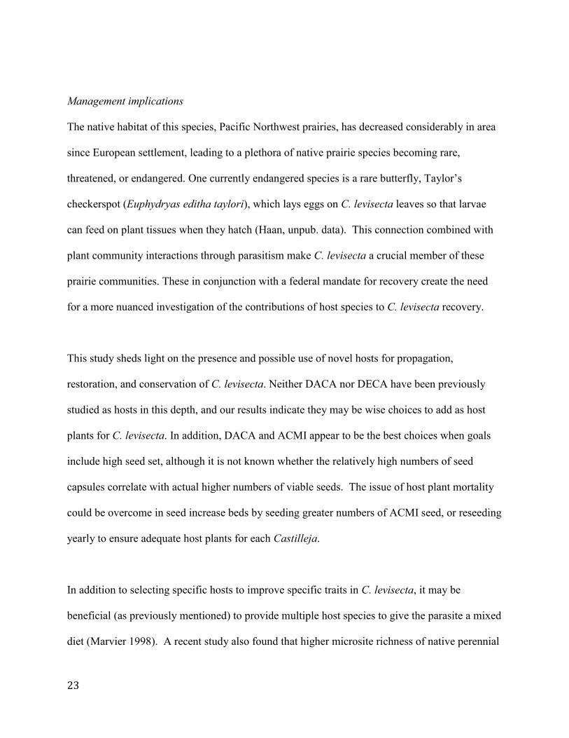
Discussion ......................................................................................................................................................... 18 Survival ........................................................................................................................................................................... 18 Growth ............................................................................................................................................................................. 18 Reproductive traits..................................................................................................................................................... 20 Overall patterns ........................................................................................................................................................... 22 Management implications ....................................................................................................................................... 23 Limitations ..................................................................................................................................................................... 24

Conclusions ...................................................................................................................................................... 24 References ........................................................................................................................................................ 26 Supplemental Materials .............................................................................................................................. 31

Chapter 3: Differences in parasites’ host-derived nutrients shown by stable isotopes of carbon and nitrogen ...................................................................................................................... 34

Abstract ............................................................................................................................................................. 34 Introduction ..................................................................................................................................................... 34 Methods ............................................................................................................................................................. 36

Study species ................................................................................................................................................................. 36 Method of nutrient measurement ........................................................................................................................ 36 Lag time pilot ................................................................................................................................................................ 37 Full experiment ............................................................................................................................................................ 37 Isotope labelling .......................................................................................................................................................... 38 Analysis ........................................................................................................................................................................... 40

Results ............................................................................................................................................................... 40 Carbon ............................................................................................................................................................................. 40 Nitrogen .......................................................................................................................................................................... 41

ii

Discussion ......................................................................................................................................................... 42 Carbon ............................................................................................................................................................................. 42 Nitrogen .......................................................................................................................................................................... 43 Study limitations ......................................................................................................................................................... 44 Implications ................................................................................................................................................................... 45

Conclusions ...................................................................................................................................................... 46 References ........................................................................................................................................................ 47 Appendix 3.1: Lag time pilot experiment .............................................................................................. 49

Chapter 4: Do all parasitic plants work as ecosystem engineers? A case study in Pacific Northwest prairies ............................................................................................................... 52

Abstract ............................................................................................................................................................. 52 Introduction ..................................................................................................................................................... 52 Methods ............................................................................................................................................................. 54

Study species and site ............................................................................................................................................... 54 Analysis ........................................................................................................................................................................... 55

Results ............................................................................................................................................................... 58 Community composition .......................................................................................................................................... 58 Species richness ........................................................................................................................................................... 60 Lag time ........................................................................................................................................................................... 61

Discussion ......................................................................................................................................................... 64 Conclusions ...................................................................................................................................................... 67 References ........................................................................................................................................................ 69 Supplemental materials .............................................................................................................................. 72

Chapter 5: Synthesis ........................................................................................................................... 75

All References ....................................................................................................................................... 78

Appendix A: ‘R’ code used for Chapter 2 analyses ................................................................... 85

Appendix B: ‘R’ code used for Chapter 3 analyses ................................................................... 91

Appendix C: ‘R’ code used for Chapter 4 analyses ................................................................... 93

iii

List of Figures

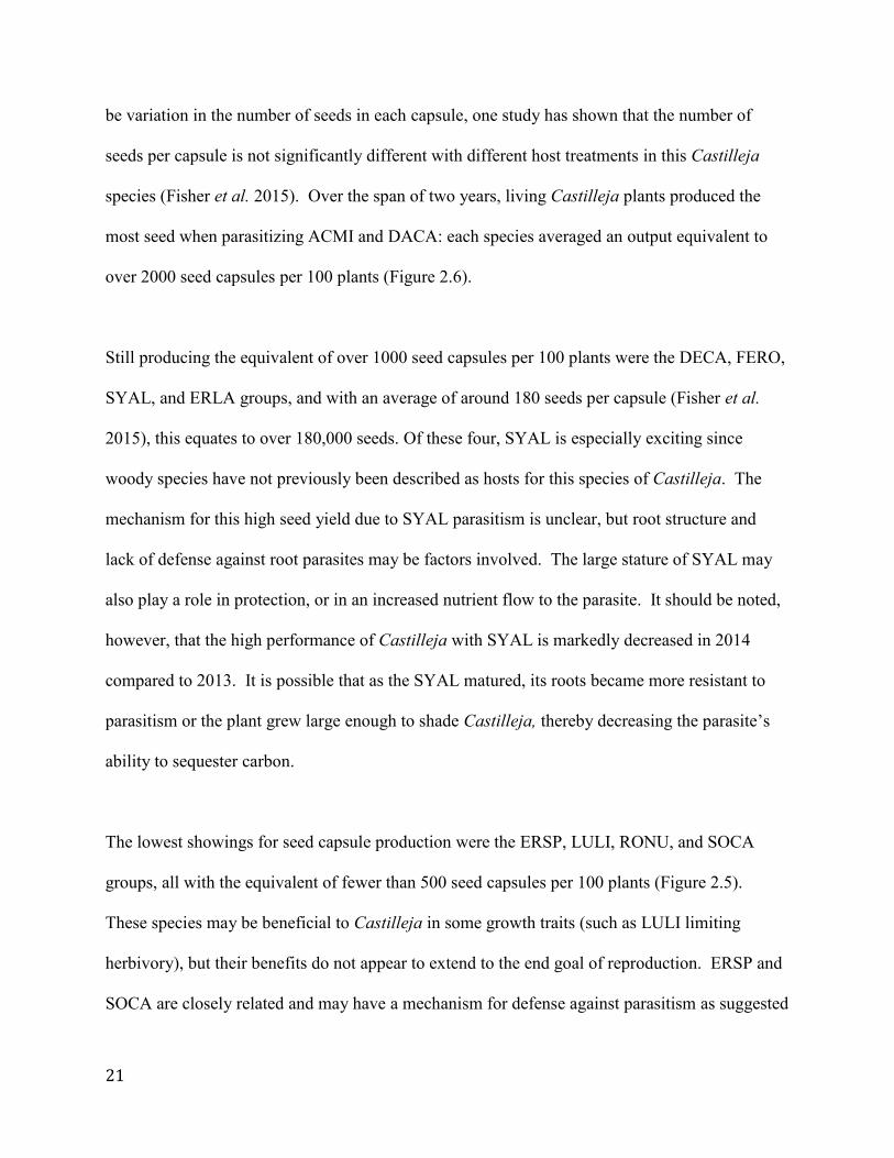
Figure 2.1 Castilleja levisecta parasitizing Rumex acetosella. Darker root is R. acetosella and

lighter root (with haustorium) is C. levisecta……………………………........................….……..5

Figure 2.2 Percent survival of Castilleja-host pairs over two years of study. Survival was only

counted when both plants in the pair were alive at the time of sampling. See Table 2.1 for full

species names…………………………………………………………………………………….11

Figure 2.3 Height of Castilleja in 2013 and 2014 by host species. Data were only included from

live pairs. Dotted lines indicate the nominal range of the data inferred from the upper and lower

quartiles (box edges). Points that fall outside this range are shown as open circles. See Table 2.1

for full species names.....................................................................................................................12

Figure 2.4 Percent of live Castilleja plants that were browsed in each treatment group. While a

generalized liner model showed that number of browsed plants differed by host, only marginal

(p>0.05) differences appeared in pairwise comparisons. Data were only included from live pairs.

See Table 2.1 for full species names.………………………………........................................….13

Figure 2.5 Number of Castilleja seed capsules in 2013 and 2014 by host species. Data were only

included from live pairs. See Table 2.1 for full species names and Figure 2.3 for plot

description......................................................................................................................................15

Figure 2.6 Sum of 2013 and 2014 total seed capsule averages in Castilleja plants, by host.

Castilleja in the no host treatment did not have any capsule production in 2013, and no

significant production in 2014. See Table 2.1 for full species names............……..……………16

Figure S2.1 Flowering stems of Castilleja in 2013 and 2014 by host species. Circles indicate

outliers, some of which were removed to improve scaling (DECA, y = 25, and ERLA, y = 46).

Data were only included from live pairs. See Table 2.1 for full species names and Figure 2.3 for

plot description...............................................................................................................................32

Figure S2.2 Browsed stems of Castilleja in 2013 and 2014 by host species. Circles indicate

outliers. Data were only included from live pairs. See Table 2.1 for full species names and Figure

2.3 for plot description...................................................................................................................32

Figure S2.3 Fruiting stems of Castilleja in 2013 and 2014 by host species. Data were only

included from live pairs. Circles indicate outliers. See Table 2.1 for full species names and

Figure 2.3 for plot description.......................................................................................................33

Figure 3.1 Schematic showing labeled carbon and nitrogen addition to host plant parasitized by

Castilleja levisecta………………………………….……………………………………………39

Figure 3.2 Median del values of 13C in Castilleja by host species. Letters represent grouping by

significant differences (p<0.05)..…………….………………………………………………..…41

iv

Figure 3.3 Median del values of 15N in Castilleja by host species. Letters represent grouping by

significant differences (p<0.05)..…………….………………………………………………..…42

Figure S3.1 Del 15N values of Castilleja (CALE) and host species in days following label

addition to host plant..……………..................................................................………………..…51

Figure S3.2 Del 13C values of Castilleja (CALE) and host species in days following label

addition to host plant....……………................................................................………………..…51

Figure 4.1 Ordisurf plots of Castilleja plant density (bubble size) and community composition

(bubble placement) from PERMANOVA analysis of 2011 density and 2012 composition at each

site. Density ranges (bubble sizes) are as follows: EL (0-11), GH (2-22), SP (0-6), and WR (1-

14)..................................................................................................................................................60

Figure 4.2 Years between measurement of density (e.g. 2011) and richness/composition (e.g.

2014), and variation in species richness and composition attributed to Castilleja density.

Overlapping values were spaced using “jitter” function. Filled markers indicate northern sites

(Ebey’s Landing and Smith Prairie), hollow markers indicate southern sites (Glacial Heritage

and West Rocky)............................................................................................................................62

Figure 4.3 Density of Castilleja in 2011 and quadrat species richness in 2012 at each site. It

should be noted that these are actual quadrat-level values, not averages, and only the Ebey’s

Landing comparison was statistically significant..........................................................................63

Figure 4.4 Density of Castilleja and species richness in significant (p<0.05, top) and marginally

significant (p<0.07) analyses. It should be noted that these are actual quadrat-level values, not

averages..........................................................................................................................................64

Figure S4.1 Castilleja density in each quadrat by site in 2011. Dotted lines indicate the nominal

range of the data inferred from the upper and lower quartiles (box edges). Points that fall outside

this range are shown as open circles..............................................................................................72

Figure S4.2 Castilleja density in each quadrat by site in 2012. See Figure S4.1 for plot

description......................................................................................................................................73

Figure S4.3 Castilleja density in each quadrat by site in 2013. See Figure S4.1 for plot

description......................................................................................................................................74

v

List of Tables

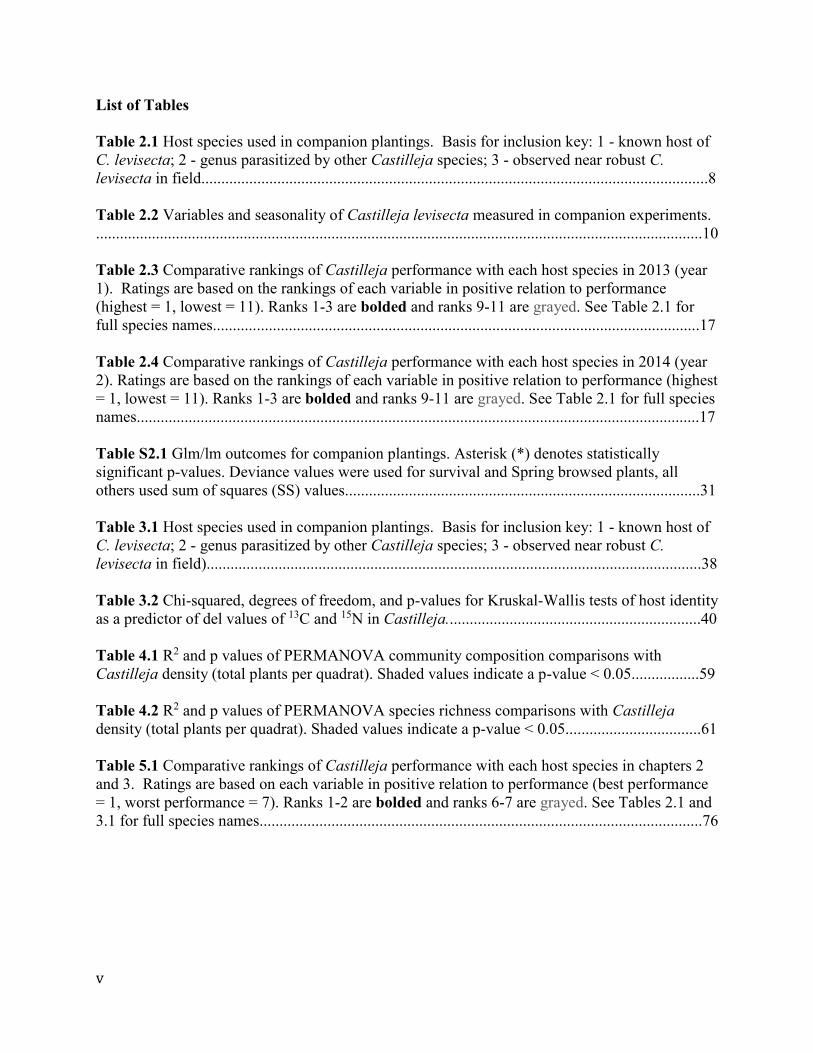
Table 2.1 Host species used in companion plantings. Basis for inclusion key: 1 - known host of

C. levisecta; 2 - genus parasitized by other Castilleja species; 3 - observed near robust C.

levisecta in field...............................................................................................................................8

Table 2.2 Variables and seasonality of Castilleja levisecta measured in companion experiments.

........................................................................................................................................................10

Table 2.3 Comparative rankings of Castilleja performance with each host species in 2013 (year

1). Ratings are based on the rankings of each variable in positive relation to performance

(highest = 1, lowest = 11). Ranks 1-3 are bolded and ranks 9-11 are grayed. See Table 2.1 for

full species names..........................................................................................................................17

Table 2.4 Comparative rankings of Castilleja performance with each host species in 2014 (year

2). Ratings are based on the rankings of each variable in positive relation to performance (highest

= 1, lowest = 11). Ranks 1-3 are bolded and ranks 9-11 are grayed. See Table 2.1 for full species

names.............................................................................................................................................17

Table S2.1 Glm/lm outcomes for companion plantings. Asterisk (*) denotes statistically

significant p-values. Deviance values were used for survival and Spring browsed plants, all

others used sum of squares (SS) values.........................................................................................31

Table 3.1 Host species used in companion plantings. Basis for inclusion key: 1 - known host of

C. levisecta; 2 - genus parasitized by other Castilleja species; 3 - observed near robust C.

levisecta in field)............................................................................................................................38

Table 3.2 Chi-squared, degrees of freedom, and p-values for Kruskal-Wallis tests of host identity

as a predictor of del values of 13C and 15N in Castilleja................................................................40

Table 4.1 R2 and p values of PERMANOVA community composition comparisons with

Castilleja density (total plants per quadrat). Shaded values indicate a p-value < 0.05.................59

Table 4.2 R2 and p values of PERMANOVA species richness comparisons with Castilleja

density (total plants per quadrat). Shaded values indicate a p-value < 0.05..................................61

Table 5.1 Comparative rankings of Castilleja performance with each host species in chapters 2

and 3. Ratings are based on each variable in positive relation to performance (best performance

= 1, worst performance = 7). Ranks 1-2 are bolded and ranks 6-7 are grayed. See Tables 2.1 and

3.1 for full species names...............................................................................................................76

vi

Acknowledgements

I am grateful to my advisor, Jon Bakker, for his continued patience, support, and mentorship

throughout the past five years. I am also thankful to my committee members, Kern Ewing, Sarah

Hamman, Peter Dunwiddie, Soo-Hyung Kim, Dick Olmstead, and Janneke Hille Ris Lambers,

who each inspired me and provided valuable comments over the course of my degree. I am

forever indebted to my past and current labmates, who all helped me on my path in various ways.

Especially Eric Delvin, whose epic research provided the data used in Chapter 4, Rachel

Mitchell, who is hilarious and gave me someone to aspire to, and Loretta Fisher, who will remain

my lifelong friend. Also of tremendous service were my lab assistants: Del Brummet, Will

Mooreston, Ben Saari, and Rae Mecka. I could not have done all this without your help. I would

also like to thank the Center for Natural Lands Management and the Center for Urban

Horticulture for their contribution of time and resources, and I am grateful for the great help and

pleasing demeanor of Mark Roth on those cold out-planting days. I am thankful to have received

support from the University of Washington’s Royalty Research Fund, the United States Fish and

Wildlife Service, and the Washington State Federation of Garden Clubs (WSFGC) Scholarship.

Finally, I would like to thank my family. My parents, Cathy and Dave, have always supported

me and were a pillar of strength through the ups and downs of this process. My brother,

Andrew, pushed me to achieve by his own achievements, and continues to put my brain to the

test. And lastly, my dear husband Chris Jones. I could not have done this without you. Many

worlds we’ve come since we first left home.

vii

Note to the reader: Chapters 2-4 are intended as separate manuscripts for publication.

Therefore, each includes an abstract, appendices, and a stand-alone references section, and

“we” language is used in place of “I.” Target journals include Northwest Science (Chapter 2),

New Phytologist (Chapter 3), and Ecological Processes (Chapter 4).

1

Chapter 1: An introduction to research on Castilleja levisecta and Pacific Northwest

prairies

Parasitic angiosperms occupy a unique niche in the ecosystems they inhabit (Press and Phoenix

2005). They are present in systems throughout the world and are regarded as agricultural pests

as well as ecosystem engineers (Watson 2009). Research at present is embarking on a better

understanding of the latter role, and recent studies have shown potential for parasitic plants to be

used in the restoration of degraded ecosystems (e.g. Westbury et al. 2006).

This potential for restoration is of special interest when the parasite itself is a threatened species,

as is the case with Castilleja levisecta. This root hemiparasite has been extirpated in most of its

native range from British Columbia to Oregon (Caplow 2004). Much of this loss has been linked

to habitat loss, as Pacific Northwest prairies now occupy less than 10% of their historical area

(Crawford and Hall 1997). In the process of restoration of this individual species it is possible

that restorative effects will also be observed in the greater plant community.

We conducted three experiments to examine the potential for restoration benefits to Castilleja

levisecta and Pacific Northwest prairies. In the first, C. levisecta was planted in the field with

one of eleven known or potential host species. For two years we monitored each parasite for

survival, growth, and reproduction, and used these data to determine differences between host

species contributions to Castilleja. In the second study, seven host species were planted with C.

levisecta and labelled with heavy isotopes of carbon and nitrogen. We allowed the isotopes to

travel from the host to the parasite, then sampled Castilleja to establish differences in relative

nutrition received from each host species. The third study used community composition data

from a multi-year prairie experiment to test the effects of parasite density on the prairie

2

community. We used PERMANOVA to test this effect with four years of data from four sites in

western Washington.

3

Chapter 2: Host species influence on growth and reproduction of threatened hemiparasite

Castilleja levisecta

Abstract

Restoration of a threatened species requires an understanding of the life history and resources

necessary to facilitate the establishment and reproduction of new populations. Pacific Northwest

native Castilleja levisecta (Orobanchaceae) is a facultative hemiparasite: it prefers but does not

require a host to complete its life cycle, and it is able to sequester carbon via photosynthesis.

The aim of this study was to elucidate the most useful host species for growth and reproduction

of this parasite. We used host-parasite pairs in a two-year field study to compare the effects of a

variety of host species. Our data show that host identity affects survival, and growth and

reproductive traits of Castilleja levisecta. Furthermore, the two host species widely cited in the

literature, Eriophyllum lanatum and Festuca roemeri, were not always the top performers in our

group of hosts, and in many cases Achillea millefolium was among the top treatments for

Castilleja performance. Thus, Achillea and other novel hosts should be considered for use in

preservation and reintroduction of Castilleja levisecta.

Introduction

Parasitic plants make up nearly 1% of angiosperms in the world and are present in nearly every

biome (Nickrent et al. 1998, Press and Phoneix 2005). Some parasitic plants are detrimental to

crops, (i.e. Striga), while others appear to have positive and often complex influences on their

communities (Bao et al. 2015, Fisher et al. 2013). This influence is not limited to the plants they

parasitize and can extend to higher trophic levels, affecting invertebrates as well as other non-

host species (Hartley et al. 2015). As a result, parasitic angiosperms often have effects on their

communities that are greater than expected given their biomass, and have been proposed as

4

keystone species and ecosystem engineers (Rowntree et al. 2014, Watson 2009). In this light, it

is crucial to understand the role of parasites in their native systems and the interactions with

which they directly and indirectly influence the community around them.

Castilleja levisecta (golden paintbrush) is a federally threatened parasite native to Washington,

Oregon, and British Columbia. This species, as with all plants in the genus Castilleja, attaches to

hosts using parasitic root structures, called haustoria, which facilitate a xylem-xylem connection

between the parasite and its host (Kuijt 1969, shown in Figure 2.1). As a facultative

hemiparasite, Castilleja is able to survive and reproduce without a host and is also able to

sequester its own carbon via photosynthesis (Wentworth 2001). Despite this ability to live

without host resources, many studies have shown considerable increases in hemiparasite growth

and reproductive traits in the presence of a host plant, and in some cases a large proportion of the

parasite’s total carbon is host-derived (Pageau et al. 1998).

Host species identity appears to play a major role in the survival and overall performance of

Castilleja levisecta (Delvin 2013, Lawrence and Kaye 2008). Several studies of host influence

have been conducted, mainly comparing the host quality of Eriophyllum lanatum and Festuca

roemeri (e.g Lawrence and Kaye 2008). However, little has been done to investigate the effects

of host identity on Castilleja levisecta using a wide range of hosts. And while functional group

may sometimes be a predictor of host quality (Lawrence and Kaye 2011), studies in other

systems have shown that species-level differences, not functional groups, are better predictors of

hemiparasite performance based on host identity (Demey et al. 2015, Rowntree et al. 2014). If

we are to truly understand the nature of Castilleja’s relationship with different hosts for the

5

ultimate goal of restoration, we are obliged to examine numerous diverse host species and their

effects on parasite growth and reproduction.

Recent studies (e.g. Kaye et al. 2011) have begun to explore the possibility of host species

beyond Eriophyllum lanatum and Festuca roemeri. Ecologists monitoring extant C. levisecta

populations have also noticed some individuals thriving in the absence of these two known hosts

(Dunwiddie and Bakker, pers. comm.). This suggests that C. levisecta may be able to parasitize

a wide variety of hosts, which is consistent with our understanding of the genus Castilleja as

generalist parasites (Dobbins and Kuijt 1973, Heckard 1962).

One study found that C. levisecta grown with Achillea millefolium were significantly larger than

controls and those grown with other hosts, including Festuca roemeri (Kaye et al. 2011). This

6

study also tested Danthonia californica as a possible host, but results were not significantly

different from no-host controls. Personal observations by researchers working with C. levisecta

have led to speculation that Rosa nutkana, Symphoricarpos albus, and Erigeron speciosus may

also be viable hosts (Dunwiddie and Bakker, pers. comm.). Research also suggests that C.

levisecta has higher survival when planted with a perennial host species (Lawrence 2005), and

that in some cases, plantings with known host Eriophyllum lanatum have decreased C. levisecta

survival compared to controls with no host (Lawrence and Kaye 2008).

Other species of hemiparasitic Castilleja have been known to acquire defensive compounds from

host plants (especially composites and legumes) through haustorial connections (Stermitz and

Harris 1987, Marko and Stermitz 1997). This type of transfer could increase the ability of C.

levisecta to withstand herbivory and decrease mortality in out-planting sites. Adler (2003) also

found that Castilleja indivisa parasitizing a lupine species gained reproductive advantages

(increased seed production and increased visitation by pollinators) over those parasitizing a

graminoid species.

In light of this species’ potential to parasitize a wide range of host species, and the mixed and

sometimes conflicting results gleaned from literature review, we tested a variety of known and

novel host species to assess their effect on the survival, growth, and reproduction of Castilleja

levisecta. We also tested over a two-year period in order to measure changes in these effects

over time. This improves our understanding of not only the breadth of hosts parasitized by this

species, but also our knowledge of potential new directions for recovery and preservation of

7

current populations. To this end, the objective of this study was to identify the host species that

enable Castilleja levisecta to survive, grow, and ultimately reproduce most effectively.

Methods

This experiment used what we refer to as “companion plantings.” This method pairs a single

parasite individual with a single host individual in a field planting. Control pairings contained

two Castilleja levisecta (CALE) individuals to account for competition but remove parasitism.

Parasites and host plants were grown from seed (except for woody species) in a greenhouse

setting for 4 months prior to planting. Seeds were germinated according to established methods

in growth chambers then transplanted into greenhouse plug trays for establishment. Woody

species were propagated vegetatively by cuttings obtained from the Union Bay Natural Area

(Seattle, WA). Cuttings were dipped in rooting hormone prior to striking and trays were placed

on a mist bench for 1-2 weeks for root establishment, followed by normal greenhouse growth

with the seeded species. All individual plants were grown in separate plugs prior to outplanting

in the field for ease of transport (as in Schmidt 1998).

Companion pairs were planted at Glacial Heritage Preserve (Littlerock, WA), a former

agricultural site that is currently the location of restoration and preservation efforts of Pacific

Northwest prairies. We used twenty replicates of each unique host-parasite pairing. The pairs

were planted in the fall of 2012, host and parasite in the same hole, with roots touching. All pairs

were measured in the spring and fall of 2013 and 2014. They were set up on a grid with one

meter between each pair to discourage CALE from attaching to individuals other than the host

8

being tested, and ordering of pairs was randomized. All pairs were weeded in the spring of 2013

and 2014.

Table 2.1 Host species used in companion plantings. Basis for inclusion key: 1 - known host of

C. levisecta; 2 - genus parasitized by other Castilleja species; 3 - observed near robust C.

levisecta in field.

Species Species

abbreviation Family Functional

Group

Basis for

inclusion

Achillea millefolium ACMI Asteraceae Forb 1

Danthonia californica DACA Poaceae Grass 1

Deschampsia caespitosa DECA Poaceae Grass 1

Erigeron speciosus ERSP Asteraceae Forb 1

Eriophyllum lanatum ERLA Asteraceae Forb 1

Festuca roemeri FERO Poaceae Grass 1

Lupinus lepidus LULE Fabaceae Legume 1

Lupinus littoralis LULI Fabaceae Legume 2

Rosa nutkana RONU Rosaceae Shrub 3

Solidago canadensis SOCA Asteraceae Forb 1

Symphoricarpos albus SYAL Caprifoliaceae Shrub 3

Host species used in the study were chosen for a variety of reasons, detailed in Table 1 above,

and represent a diversity of families and functional groups. ERLA and FERO have been

documented extensively in the literature as hosts of C. levisecta (e.g. Lawrence and Kaye 2008).

Additional hosts (ACMI, DACA, DECA, ERSP, LULE, SOCA) have been tested in our

greenhouse facilities, where we found haustorial connections between these species and C.

levisecta (Schmidt, unpub. data). The two woody species (RONU and SYAL) used in this study

are found in Pacific Northwest prairies and have been noted in proximity to robust C. levisecta

populations where few other potential hosts are present. Lastly, in an attempt to widen the pool

of potential hosts, an additional Lupinus species (LULI) was added to observe potential

differences in host suitability with two nitrogen-fixing hosts.

9

Measured variables

Measurements were conducted in spring and fall of 2013 and 2014 (Table 2.2). Survival was

counted positively when both the host plant and the parasite survived. Then, using those pairs

that survived, we measured additional variables of the Castilleja individuals. In the spring, we

began by measuring the number of flowering stems as a metric of potential reproductive

capacity. However, deer browse occurred on the site, leading us to additionally measure browsed

stems and the number of surviving plants browsed to assess changes in reproductive potential

and overall growth. Another growth trait, height, was determined by measuring the length of the

longest stem. In the fall we returned to the site and measured the final reproductive output for

that growing season: number of fruiting stems (stems that had at least one seed capsule) and the

total number of seed capsules per plant.

10

Table 2.2 Variables and seasonality of Castilleja levisecta measured in companion experiments.

Measurement Measurement season Trait category Model type

Survival (y/n) Spring Survival Binomial

Number of flowering

stems Spring Reproductive Poisson

Number of browsed

stems Spring Growth/Reproductive Poisson

Plants browsed (y/n) Spring Growth/Reproductive Binomial

Height Spring Growth Poisson

Number of fruiting

stems Fall Reproductive Poisson

Number of seed

capsules Fall Reproductive Poisson

Statistical Analyses

For each year, each trait was compared with host identity using generalized linear models (glm)

and linear models (height only – both years) to test for differences between host groups and the

control (two parasites with no host). Survival and number of browsed plants were tested with a

glm using a binomial distribution, while all other variables (except height) were tested with a

glm using a poisson distribution. We tested the effect of host treatment on each response

variable, followed by pairwise comparisons among hosts. Traits other than survival used data

only from those host-parasite pairs that survived in that year. This should be noted when

interpreting comparisons in performance between hosts, as some hosts may have a significant

effect on surviving Castilleja but a low percentage of overall survival, and some Castilleja

survived even when the host died. Analyses were conducted using R statistical software (version

3.1.3, Appendix A). For a qualitative analysis, we also ranked the mean values of each trait by

11

host species to create a table that visually represented the performance of Castilleja with each

host.

Results

Survival

Our companion experiment resulted in a range of variation of CALE survival. Survival ranged

from 11% (Solidago canadensis group in 2014) to 74% (Deschampsia caespitosa in 2013),

(Figure 2.2). Survival in the LULE treatment group was zero in both years, so it was removed

from the remainder of the analyses. At the end of the experiment, DACA and DECA treatment

groups had the highest survival, followed by ERLA, FERO, ACMI, LULI, and the no host

control group. The lowest survival was in the RONU, SYAL, ERSP, and SOCA treatment

groups.

12

Growth

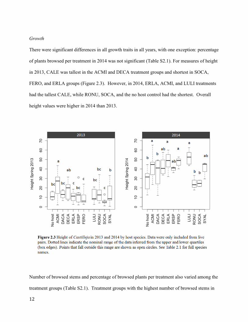
There were significant differences in all growth traits in all years, with one exception: percentage

of plants browsed per treatment in 2014 was not significant (Table S2.1). For measures of height

in 2013, CALE was tallest in the ACMI and DECA treatment groups and shortest in SOCA,

FERO, and ERLA groups (Figure 2.3). However, in 2014, ERLA, ACMI, and LULI treatments

had the tallest CALE, while RONU, SOCA, and the no host control had the shortest. Overall

height values were higher in 2014 than 2013.

Number of browsed stems and percentage of browsed plants per treatment also varied among the

treatment groups (Table S2.1). Treatment groups with the highest number of browsed stems in

13

2013 were ACMI, ERSP, and the no host control, while the lowest numbers were found in the

LULI, RONU, and SOCA groups (Figure S2.2). However, in 2014, the ERSP group dropped to

one of the lowest numbers of browsed stems, along with RONU and SYAL. The no host control,

DACA, and ACMI groups had among the highest percentages of live plants browsed in both

2013 and 2014 (Figure 2.4). DECA and ERLA had a relatively lower percentage of plants

browsed in 2013 but increased significantly in 2014, while ERSP had relatively high browse in

2013 and lower in 2014. LULI, RONU, SOCA, and SYAL treatment groups remained in the

lower relative percentages of browse in both years. Overall percent of plants browsed increased

from 2013 to 2014 (Figure 2.4).

14

Reproduction

Flowering stems were significantly different based on host identity (Table S2.1). In 2013, The

ACMI and DECA groups had the highest number of flowering stems, and the no host control had

the lowest (Figure S2.1). Castilleja in the DECA treatment remained with relatively high

numbers of flowering stems in 2014, and the ERLA group rose to the top performer for this trait.

The control group remained in the lower relative numbers, joined by the RONU and SOCA

groups.

Fruiting stems showed a similar response to host treatment: the ERLA group had lower numbers

in 2013 but rose to be one of the top performers in 2014 (Figure S2.3). ACMI was a top

performer in both years, as was DACA. One difference from flowering stems was the SYAL

treatment, which was the top group in 2013 and remained among the top performers in 2014.

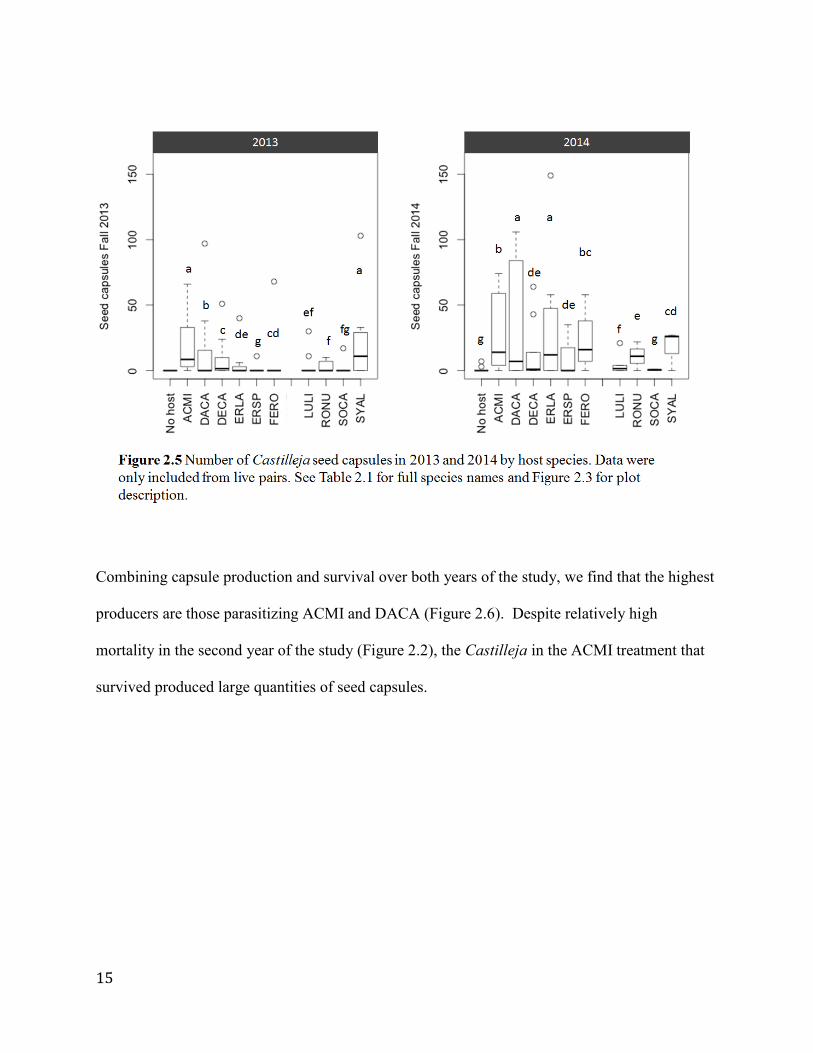
Seed capsule output, the trait that most directly assessed reproduction, showed a wide range of

values (Figure 2.5). Castilleja in the SYAL and ACMI groups produced more capsules in the

first year of the experiment, while the ERSP had the lowest (and the no host control had no

capsules in 2013). In 2014, the DACA and ERLA groups had the most seed capsules, while the

SOCA and control groups had the least. For the most part, treatment groups had similar or

increased average capsule outputs in 2014, with the exception of SOCA and SYAL, which

decreased their average capsule number in the second year of the study.

15

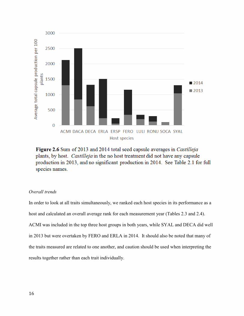
Combining capsule production and survival over both years of the study, we find that the highest

producers are those parasitizing ACMI and DACA (Figure 2.6). Despite relatively high

mortality in the second year of the study (Figure 2.2), the Castilleja in the ACMI treatment that

survived produced large quantities of seed capsules.

16

Overall trends

In order to look at all traits simultaneously, we ranked each host species in its performance as a

host and calculated an overall average rank for each measurement year (Tables 2.3 and 2.4).

ACMI was included in the top three host groups in both years, while SYAL and DECA did well

in 2013 but were overtaken by FERO and ERLA in 2014. It should also be noted that many of

the traits measured are related to one another, and caution should be used when interpreting the

results together rather than each trait individually.

17

Table 2.3 Comparative rankings of Castilleja performance with each host species in 2013 (year

1). Ratings are based on the rankings of each variable in positive relation to performance

(highest = 1, lowest = 11). Ranks 1-3 are bolded and ranks 9-11 are grayed. See Table 2.1 for

full species names.

2013 Survival Flowering

stems

Browsed

stems

Plants

browsed Height

Fruiting

stems

Seed

capsules

Average

rank

ACMI 2 1 1 10.5 1 2 2 2.79

DACA 3 7 4 9 5 3 3 4.86

DECA 1 3 8 4 2 4.5 4 3.79

ERLA 7 9.5 5 6.5 10 7 6 7.29

ERSP 10 5 2 10.5 6 8 10 7.36

FERO 7 9.5 6 6.5 9 6 5 7.00

LULI 4.5 6 10 2 7 10 8 6.79

RONU 9 4 10 2 4 4.5 7 5.79

SOCA 7 11 10 2 11 9 9 8.43

SYAL 4.5 2 7 5 3 1 1 3.36

No host 11 8 3 8 8 11 11 8.57

Table 2.4 Comparative rankings of Castilleja performance with each host species in 2014 (year

2). Ratings are based on the rankings of each variable in positive relation to performance (highest

= 1, lowest = 11). Ranks 1-3 are bolded and ranks 9-11 are grayed. See Table 2.1 for full species

names.

2014 Survival Flowering

stems

Browsed

stems

Plants

browsed Height

Fruiting

stems

Seed

capsules

Average

rank

ACMI 5.5 6 1 11 4 1 3 4.50

DACA 2 7 3 8 8 4 1 4.71

DECA 1 2 6 7 5 6 6 4.71

ERLA 3 1 2 9 2 2 2 3.00

ERSP 8.5 5 11 3 7 8 7 7.07

FERO 4 4 5 6 3 3 4 4.14

LULI 5.5 8 8.5 3 1 8 9 6.14

RONU 8.5 9 8.5 3 10 8 8 7.86

SOCA 8.5 11 7 3 11 10 10 8.64

SYAL 8.5 3 10 3 6 5 5 5.79

No host 7 10 4 10 9 11 11 8.86

18

Discussion

Survival

Survival was somewhat low in general, although our methods tended to overestimate mortality.

Because only pairs in which host and Castilleja survived were counted, it is possible that

multiple pairs with living Castilleja were not counted due to host plant mortality. In our

observations over the course of the experiment, some treatments (such as ACMI) had a large

drop in host survival after the first year, with many Castilleja still alive. Conversely, groups

such as SOCA had more host survival combined with Castilleja mortality. This may point to

outside environmental factors influencing host-parasite interactions, or host plant mortality in

some cases may have been due to the strength of parasitism reducing the host plants’ ability to

survive. Similarly, high host survival rates could be a sign of a poor host, as it may not be

adversely affected by parasitism. This could also be due to differences in host species’ ability to

resist parasitism, as has been documented with European hemiparasite Rhinanthus minor

(Cameron et al. 2006). In that case, rather than being a selective difference mitigated by the

parasite, the host’s resistance created a barrier to parasitism and greatly reduced nutrient

acquisition by the parasite. This mechanism may be present in the grass species we studied, as

Poaceae is known to have resistance to parasitism but the strength of resistance varies by species

(Rümer et al. 2007).

Growth

Castilleja in the ACMI treatment were consistently high performers in height, but had a

relatively high percentage of live plants browsed. While they also had a relatively high number

19

of browsed stems, this could be considered a positive: that there were a high number of stems

available to be browsed means that the plants had a high level of growth (possibly due to host

resources) to begin with. This native forb is prevalent in Pacific Northwest prairies and can be

easily seeded into restoration and preservation areas. It has recently been suggested that clonally

spreading species may be easier targets for parasitism (Demey et al. 2015), and this may be one

of the underlying mechanisms for ACMI’s high performance as a host since it spreads clonally.

Root structure in general may play a large part in the ability of parasites to form and maintain

haustoria, and future studies of this nature should consider categorizing root structures of each

host species in addition to other measures.

The ERLA, DECA, and DACA host groups also performed relatively well: they were among the

tallest average Castilleja in 2014 and also had more browsed stems in 2014 (Figures 2.3 and

S2.2). However, all of these treatment groups had more than 50% of the live Castilleja plants

browsed in 2014. ERLA is a known host of Castilleja (Lawrence and Kaye 2008), but DACA

and DECA have not been widely studied as hosts for this species.

Number of browsed stems and percent of plants browsed fluctuated considerably between the

two years of measurement (Figures 2.4 and S2.2). Castilleja in the LULI, RONU, and SOCA

treatments were not browsed at all in 2013, but all three groups had over one quarter of their live

Castilleja browsed in 2014. It is possible that different host-derived compounds are acquired or

are more important in different growth stages of CALE, as has been observed with Striga

hermonthica (Aflakpui et al. 2005, Pageau 1998). Despite the increase in browse in 2014, these

20

three host groups remain among the lowest relative percentages of live plants browsed per

treatment.

The hosts associated with lower Castilleja browse may have conferred extra-nutritional benefits

to the CALE parasitizing them, such as defensive compounds dissolved in xylem sap, or

protection from herbivory by mechanical means. Lupines are known in some cases to produce

bitter alkaloids which limit herbivory, and these compounds are sometimes passed on to parasites

(Adler 2002, Adler 2003). For example, several studies show that other species of Castilleja

receive quinolizidine alkaloids when parasitizing various species of lupines, but lack these

compounds when using other species as hosts (Stermitz and Harris 1987, Stermitz and Pomeroy

1986, Adler and Wink 2001). This may be the case with the LULI in our study. However, our

other lupine species, LULE, had no surviving pairs in either year of the study. Thus, these

effects may vary significantly by lupine species. The RONU hosts may have limited herbivory

by spine production, making an attempt to eat the shorter Castilleja plants a painful proposition.

In the case of SOCA, it is unclear whether the abundant foliage hid Castilleja from the sights of

herbivores, or a defensive compound of some kind was provided through parasitism.

Reproductive traits

An additional metric of value for restoration and conservation is the overall output of seed from

each host treatment. This helps to determine a population’s ability to persist and replenish plants

following mortality. To this end, we plotted the sum of seed capsule averages (per all plants,

including those that died) in 2013 and 2014 in each treatment group to show the contribution of

seed capsules by Castilleja in that host treatment over two years (Figure 2.6). While there may

21

be variation in the number of seeds in each capsule, one study has shown that the number of

seeds per capsule is not significantly different with different host treatments in this Castilleja

species (Fisher et al. 2015). Over the span of two years, living Castilleja plants produced the

most seed when parasitizing ACMI and DACA: each species averaged an output equivalent to

over 2000 seed capsules per 100 plants (Figure 2.6).

Still producing the equivalent of over 1000 seed capsules per 100 plants were the DECA, FERO,

SYAL, and ERLA groups, and with an average of around 180 seeds per capsule (Fisher et al.

2015), this equates to over 180,000 seeds. Of these four, SYAL is especially exciting since

woody species have not previously been described as hosts for this species of Castilleja. The

mechanism for this high seed yield due to SYAL parasitism is unclear, but root structure and

lack of defense against root parasites may be factors involved. The large stature of SYAL may

also play a role in protection, or in an increased nutrient flow to the parasite. It should be noted,

however, that the high performance of Castilleja with SYAL is markedly decreased in 2014

compared to 2013. It is possible that as the SYAL matured, its roots became more resistant to

parasitism or the plant grew large enough to shade Castilleja, thereby decreasing the parasite’s

ability to sequester carbon.

The lowest showings for seed capsule production were the ERSP, LULI, RONU, and SOCA

groups, all with the equivalent of fewer than 500 seed capsules per 100 plants (Figure 2.5).

These species may be beneficial to Castilleja in some growth traits (such as LULI limiting

herbivory), but their benefits do not appear to extend to the end goal of reproduction. ERSP and

SOCA are closely related and may have a mechanism for defense against parasitism as suggested

22

above (Cameron et al. 2006). RONU, a woody species, has not previously been tested as a host

and its thicker roots may not be compatible with Castilleja’s method of parasitism. LULI, while

seeming to confer some benefits to Castilleja, does not seem to be adding nutrition that assists in

reproduction. Whether this is due to active resistance on the part of the host, or a physiological

trait within the roots that limits haustorial attachment is unknown.

Overall patterns

Changes in top performing groups over the two years of the study suggest that host influence

may fluctuate over time or based on additional factors (Tables 2.3 and 2.4). Castilleja may be

benefitted by different hosts more or less depending on life stage or environmental changes.

This has been documented in a study using Castilleja wightii in which the parasite had greater

growth and reproduction when parasitizing multiple hosts than with a single host species

(Marvier 1998). The host species with the highest management value is a subjective measure

based on which traits one is concerned with. If long-term survival is the main objective, DACA

and DECA may be the “best” hosts. If higher overall seed output is the goal, DACA and ACMI

may be superior choices.

Despite the overall high rankings of ACMI, ERLA, and FERO, it appears that some hosts are

higher performers for Castilleja’s growth traits (e.g. DECA), while others confer greater benefits

for reproduction (e.g. DACA). One implication for management is that an ecosystem with a

diversity of native prairie species may be the ideal habitat for preservation and reintroduction of

this species. It also demonstrates that more work is needed to elucidate the mechanisms of

differing benefits based on host species identity.

23

Management implications

The native habitat of this species, Pacific Northwest prairies, has decreased considerably in area

since European settlement, leading to a plethora of native prairie species becoming rare,

threatened, or endangered. One currently endangered species is a rare butterfly, Taylor’s

checkerspot (Euphydryas editha taylori), which lays eggs on C. levisecta leaves so that larvae

can feed on plant tissues when they hatch (Haan, unpub. data). This connection combined with

plant community interactions through parasitism make C. levisecta a crucial member of these

prairie communities. These in conjunction with a federal mandate for recovery create the need

for a more nuanced investigation of the contributions of host species to C. levisecta recovery.

This study sheds light on the presence and possible use of novel hosts for propagation,

restoration, and conservation of C. levisecta. Neither DACA nor DECA have been previously

studied as hosts in this depth, and our results indicate they may be wise choices to add as host

plants for C. levisecta. In addition, DACA and ACMI appear to be the best choices when goals

include high seed set, although it is not known whether the relatively high numbers of seed

capsules correlate with actual higher numbers of viable seeds. The issue of host plant mortality

could be overcome in seed increase beds by seeding greater numbers of ACMI seed, or reseeding

yearly to ensure adequate host plants for each Castilleja.

In addition to selecting specific hosts to improve specific traits in C. levisecta, it may be

beneficial (as previously mentioned) to provide multiple host species to give the parasite a mixed

diet (Marvier 1998). A recent study also found that higher microsite richness of native perennial

24

forbs was strongly correlated with C. levisecta survival and flowering (Dunwiddie and Martin

2016). This indicates that a higher number of potential hosts (native plants) broadens the diet

available to C. levisecta. Its increased performance with greater richness may imply that the

parasite gains benefit from multiple hosts at once.

Limitations

There were several limitations in this study that we hope will be overcome with future

experiments. Perhaps the greatest was the lack of distinction between host and parasite

mortality. If we had measured this factor (rather than one or both dying being uniformly

recorded as the death of the pair), we may have been better able to draw conclusions about

survival. Additionally, we would always benefit from more host species to test and larger

sample sizes. Mortality in the field will often shrink sample sizes to less than optimal, and

starting with larger numbers may curtail this issue. We also had issues with deer browse, which

may have confounded our analyses. In the future, excluding deer from the site may be an

appropriate course of action.

Conclusions

This experiment shows the range of responses of this threatened parasite to a variety of different

hosts. Castilleja appears to gain at least some benefits from a wide range of hosts and hosts differ

in the quantity and quality of their benefits, and for the most part having any host produced more

positive results than having no host.

25

The lack of a single consistent high-performing host species across all traits in the two sampling

years indicates that host contributions to Castilleja’s growth and reproduction may be variable

and potentially compounded by environmental factors. Castilleja levisecta seems to receive

growth and reproductive benefits from a range of host species, thus addition of a wide range of

native grasses, forbs, and possibly woody shrubs may be advisable in restoration and

conservation settings for optimal performance.

26

References

Adler, L.S. 2002. Host Effects on Herbivory and Pollination in a Hemiparasitic Plant. Ecology,

83(10): 2700-2710.

Adler, L.S. 2003. Host species affects herbivory, pollination, and reproduction in experiments

with parasitic Castilleja. Ecology, 84(8): 2083–2091.

Adler, L.S. and M. Wink. 2001. Transfer of alkaloids from hosts to hemiparasites in two

Castilleja-Lupinus associations: analysis of floral and vegetative tissues. Biochemical

Systematics and Ecology, 29: 551-561.

Aflakpui, G.K.S., P.J. Gregory, and R.J. Froud-Williams. 2005. Carbon (13C) and Nitrogen

(15N) translocation in a Maize-Striga hermonthica association. Experimental Agriculture, 41(3):

321-333.

Altman, B. 2011. Historical and Current Distribution and Populations of Bird Species in Prairie-

Oak Habitats in the Pacific Northwest. Northwest Science, 85: 194–222.

Boyd, R. 1999. Indians, Fire, and the Land in the Pacific Northwest. Page 320. Oregon State

University Press, Corvallis, OR.

Butchart, S.H.M. et al. 2010. Global Biodiversity: Indicators of Recent Declines. Science,

328(5982): 1164-1168.

Cameron, D.D., A. White, and J. Antonovics. 2009. Parasite–grass–forb interactions and rock–

paper– scissor dynamics: predicting the effects of the parasitic plant Rhinanthus minor on host

plant communities. Journal of Ecology, 97(6): 1311-1319.

Cameron, D.D., A.M. Coats, and W.E. Seel. 2006. Differential Resistance among Host and Non-

host Species Underlies the Variable Success of the Hemi-parasitic Plant Rhinanthus minor.

Annals of Botany, 98(6): 1289-1299.

Crawford, R. C., and H. Hall. 1997. Changes in the South Puget Sound Prairie Landscape. Pgs

11–16. Ecology and Conservation of the South Puget Sound Prairie Landscape. P.W.

Dunnwiddie and K. Ewing eds. The Nature Conservancy. Seattle, WA.

Davies, D.M., J.D. Graves, C.O. Elias, and P.J. Williams. 1997. The impact of Rhinanthus spp.

on sward productivity and composition: Implications for the restoration of species-rich

grasslands. Biological Conservation, 82(1): 87-93.

Decleer, K., D. Bonte, and R. Van Diggelen. 2013. The hemiparasite Pedicularis palustris:

‘Ecosystem engineer’ for fen-meadow restoration. Journal for Nature Conservation, 21(2): 65-

71.

27

Delvin, E. 2013. Restoring Abandoned Agricultural Lands in Puget Lowland Prairies: A New

Approach. PhD Thesis, University of Washington. Seattle, WA.

Demey, A., P. De Frenne, L. Baeten, G. Verstraeten, M. Hermy, P. Boeckx, and K. Verheyen.

2015. The effects of hemiparasitic plant removal on community structure and seedling

establishment in semi-natural grasslands. Journal of Vegetation Science, 26(3): 409-420.

Dobbins, D.R. and J. Kuijt. 1973. Studies on the haustorium of Castilleja (Scrophulariaceae). I.

The upper haustorium. Canadian Journal of Botany, 51: 917–922.

Dunwiddie, P.W. 2002. Management and restoration of grasslands on Yellow Island, San Juan

Islands, Washington, USA. Pgs 78-87. Garry Oak Ecosystem Restoration: Progress and

Prognosis. Proceedings of the Third Annual Meeting of the B.C. Chapter of the Society for

Ecological Restoration, April 27-28, 2002, P. J. Burton ed. University of Victoria. B.C. Chapter

of the Society for Ecological Restoration, Victoria, British Columbia.

Dunwiddie, P. and J.D. Bakker. 2011. Personal Communication.

Dunwiddie, P. and R.A. Martin. 2016. Microsites matter: Improving the success of rare species

reintroductions. PLoS One 11(3): e0150417.

Fazzino, L., H.E. Kirkpatrick, and C. Fimbel. 2011. Comparison of Hand-Pollinated and

Naturally-Pollinated Puget Balsamroot (Balsamorhiza deltoidea Nutt.) to Determine Pollinator

Limitations on South Puget Sound Lowland Prairies. Northwest Science, 85:352–360.

Fisher, J.P., G.K. Phoenix, D.Z. Childs, M.C. Press, S.W. Smith, M.G. Pilkington, and D.D.

Cameron. 2013. Parasitic plant litter input: a novel indirect mechanism influencing plant

community structure. New Phytologist, 198(1): 222-231.

Fisher, L., J.D. Bakker, and P.W. Dunwiddie. 2015. An Assessment of Seed Production and

Viability of Putative Castilleja levisecta × C. hispida Hybrids. Report for the Center for Natural

Lands Management.

Franklin, J. F., and C. T. Dyrness. 1988. Natural vegetation of Oregon and Washington. Oregon

State University Press.

Grewell, B.J. 2008. Hemiparasites generate environmental heterogeneity and enhance species

coexistence in salt marshes. Ecological Applications, 18(5): 1297-1306.

Gurney, A.L., D. Grimanelli, F. Kanampiu, D. Hoisington, J.D. Scholes, and M.C. Press. 2003.

Novel sources of resistance to Striga hermonthica in Tripsacum dactyloides, a wild relative of

maize. New Phytologist, 160(3): 557-568.

Haan, N. 2015. Unpublished data.

28

Hartley, S.E., J.P. Green, F.P. Massey, M.C.P. Press, A.J.A. Stewart, and E.A. John. 2015.

Hemiparasitic plant impacts animal and plant communities across four trophic levels. Ecology,

96(9): 2408-2416.

Hautier, Y., A. Hector, E. Vojtech, D. Purves, and L.A. Turnbull. 2010. Modelling the growth of

parasitic plants. Journal of Ecology, 98(4): 857–866.

Heckard, L.R. 1962. Root parasitism in Castilleja. Botanical Gazette, 124(1): 21-29.

Kaye, T.N., K. Jones, and I. Pfingsten. 2011. Reintroduction of golden paintbrush to Oregon:

2011 Annual Report to the U.S. Fish and Wildlife Service. Institute for Applied Ecology,

Corvallis, OR.

Kuijt, J. 1969. The biology of parasitic flowering plants. University of California Press,

Berkeley, CA.

Lawrence, B.A. and T.N. Kaye. 2011. Reintroduction of Castilleja levisecta: Effects of

ecological similarity, source population genetics, and habitat quality. Restoration Ecology, 19(2):

166-176.

Lawrence, B.A. and T.N. Kaye. 2008. Direct and indirect effects of host plants: implications for

reintroduction of an endangered hemiparasitic plant (Castilleja levisecta). Madroño, 55(2): 151–

158.

Lawrence, B.A. 2005. Studies to Facilitate Reintroduction of Golden Paintbrush (Castilleja

levisecta) to the Willamette Valley, Oregon. MS thesis. Oregon State University.

Marko, M.D. and F.R. Stermitz. 1997. Transfer of alkaloids from Delphinium to Castilleja via

root parasitism. Norditerpenoid alkaloid analysis by electrospray mass spectrometry.

Biochemical Systematics and Ecology, 25(4): 279-285.

Marvier, M. 1998. A mixed diet improves performance and herbivore resistance of a parasitic

plant. Ecology, 79(4): 1272-1280.

McKinney, M.L. and J.L. Lockwood. 1999. Biotic homogenization: a few winners replacing

many losers in the next mass extinction. Trends in Ecology and Evolution 14: 450–453.

Nickrent, D.L., R.J. Duff, A.E. Colwell et al. 1998. Molecular phylogenetic and evolutionary

studies of parasitic plants. In: Soltis, DE, P.S. Soltis, J.J. Doyle, eds. Molecular Systematics of

Plants II DNA Sequencing. Boston, USA: Kluwer Academic, 211-241.

Pageau, K., P. Simier, N. Naulet, R. Robins, and A. Fer. 1998. Carbon dependency of the

hemiparasite Striga hermonthica on Sorghum bicolor determined by carbon isotopic and gas

exchange analyses. Australian Journal of Plant Physiology, 25: 695-700.

Philip, L.J. and S.W. Simard. 2008. Minimum pulses of stable and radioactive carbon isotopes to

detect belowground carbon transfer between plants. Plant Soil, 308(1-2): 23-25.

29

Phoenix, G.K. and M.C. Press. 2005. Linking physiological traits to impacts on community

structure and function: the role of root hemiparasitic Orobanchaceae (ex-Scrophulariaceae).

Journal of Ecology, 93(1): 67-78.

Press, M.C. 1998. Dracula or Robin Hood? A functional role for root hemiparasites in nutrient

poor ecosystems. Oikos, 82(3): 609-611.

Press, M.C. and G.K. Phoenix. 2005. Impacts of parasitic plants on natural communities. New

Phytologist, 166(3): 737-751.

Pywell, R.F., J.M. Bullock, K.J. Walker, S.J. Coulson, S.J. Gregory, and M.J. Stevenson. 2004.

Facilitating grassland diversification using the hemiparasitic plant Rhinanthus minor. Journal of

Applied Ecology, 41(5): 880-887.

Quested, H.M., T.V. Callaghan, J.H.C. Cornelissen, and M.C. Press. 2005. The impact of

hemiparasitic plant litter on decomposition: direct, seasonal and litter mixing effects. Journal of

Ecology, 93(1): 87-98.

Rowntree, J.K., D.F. Barham, A.J.A. Stewart, and S.E. Hartley. 2014. The effect of multiple host

species on a keystone parasitic plant and its aphid herbivores. Functional Ecology, 28(4): 829–

836.

Rümer, S., D.D. Cameron, R. Wacker, W. Hartung, & F. Jiang. 2007. An anatomical study of the

haustoria of Rhinanthus minor attached to roots of different hosts. Flora 202(3): 194–202.

Schmidt, D. 1998.Restoraion of a Prairie Ecosystem at the Yellow Island Preserve and the

Propagation of Castilleja hispida by Vegetative Cuttings. Master’s Thesis, University of

Washington. Seattle, WA.

Schultz, C.B., E. Henry, A. Carleton, T. Hicks, R. Thomas, A. Potter, M. Linders, C.

Fimbel, S. Black, H.E. Anderson, G. Diehl, S. Hamman, J. Foster, D. Hays, D.

Wilderman, R. Davenport, E. Steel, N. Page, P.L. Lilley, J. Heron, N. Kroeker, C.

Webb, and B. Reader. 2011. Conservation of Prairie-Oak Butterflies in Oregon,

Washington, and British Columbia. Northwest Science, 85: 361–388.

Severns, P.M., and A.D. Warren. 2008. Selectively eliminating and conserving exotic plants to

save an endangered butterfly from local extinction. Animal Conservation, 11(6): 476-483.

Smith, F.D., R.M. May, R. Pellew, T.H. Johnson, and K.S. Walter. 1993. Estimating extinction

rates. Nature, 364: 494–496.

Stermitz, F.R. and G.H. Harris. 1987. Transfer of pyrrolizidine and quinolizidine alkaloids to

Castilleja (Scrophulariaceae) hemiparasites from composite and legume host plants. Journal of

Chemical Ecology, 13(8): 1917-1925.

30

Stermitz, F.R. and M. Pomeroy. 1992. Iridoid glycosides from Castilleja purpurea and C.

indivisa, and quinolizidine alkaloid transfer from Lupinus texensis to C. indivisa via root

parasitism. Biochemical Systematics and Ecology, 20: 473-475.

USFWS (U.S. Fish and Wildlife Service). 2000. Recovery Plan for Golden Paintbrush (Castilleja

levisecta). U.S. Fish and Wildlife Service, Portland, Oregon.

Vitousek, P.M. 1992. Global Environmental Change - An Introduction. Annual Review of

Ecology and Systematics, 23: 1-14.

Watson, D.M. 2009. Parasitic plants as facilitators: more Dryad than Dracula? Journal of

Ecology, 97: 1151-1159.

Wentworth, J. B. 2001. The demography and population dynamics of Castilleja levisecta, a

federally threatened perennial of Puget Sound Grasslands. Pages 49–51 in R. S. Reichard, P.

Dunwiddie, J. Gamon, A. Kruckeberg, and D. Salstrom, editors. Conservation of Washington’s

Native Plants and Ecosystems. Washington Native Plant Society, Seattle.

Westbury, D.B., A. Davies, B.A. Woodcock, and N.P. Dunnett. 2006. Seeds of change: The

value of using Rhinanthus minor in grassland restoration. Journal of Vegetation Science, 17(4):

435-446.

31

Supplemental Materials

Table S2.1 Glm/lm outcomes for companion plantings. Asterisk (*) denotes statistically

significant p-values. Deviance values were used for survival and Spring browsed plants, all

others used sum of squares (SS) values.

Variable df Deviance/SS P

Survival 2013 11 -41.64 <0.0001

Spring

flowering

stems 2013 10 -60.49 < 0.0001

Spring browsed

stems 2013 10 -87.67 < 0.0001

Spring browsed

plants 2013 10 -19.78 0.0314

Height 2013 10 -2308.1 0.0007

Fall fruiting

stems 2013 9 -56.91 < 0.0001

Fall total

capsules 2013 9 -447.36 < 0.0001

Survival 2014 11 -31.71 0.0009

Spring

flowering

stems 2014 10 -118.64 < 0.0001

Spring browsed

stems 2014 10 -97.54 < 0.0001

Spring browsed

plants 2014 10 -13.15 0.2154

Height 2014 10 -4417 0.0002

Fall fruiting

stems 2014 10 -82.76 <0.0001

Fall total

capsules 2014 10 -703.68 < 0.0001

32

33

34

Chapter 3: Differences in parasites’ host-derived nutrients shown by stable isotopes of

carbon and nitrogen

Abstract

Parasitic plants are widespread and present in a variety of ecosystems across the globe. The

mechanisms by which they receive differential advantage from different hosts is not well

understood. In order to test differing nutrition as a mechanism for host suitability, we grew

hemiparasite Castilleja levisecta with one of seven host species and added stable isotopes to the

host plants. By measuring the elevated levels of the isotopes (13C and 15N) in the parasite, we

determined that nutrient acquisition does vary by host species, especially in the case of carbon.

Thus, we show that one mechanism for differential host suitability is the difference in key

nutrients gained from each host.

Introduction

Parasitic angiosperms have multiple functions within ecosystems, from invasive agricultural

pests like Striga to ecosystem engineers such as Rhinanthus. The complexity of their

interactions with their plant communities has been studied to some extent, but we lack a more

sophisticated understanding of the specifics within host-parasite interactions of non-pest species.

While it is of critical importance to investigate the mechanisms of problem parasites for the

purpose of resistance or eradication, it still remains important to study those parasites that are not

pests, or even may be contributing positive influences to a system.

In particular, the differences in host plants’ contribution to many parasites’ growth is not well

understood. Hemiparasites are often selective in the host species they parasitize, in that their

attachment to hosts near them is often non-random (Suetsugu et al. 2008). Many parasitic plants

35

appear to have “preferred” hosts which give a greater advantage to the parasite than other

available hosts (Alder 2003, Li et al. 2013). These hosts may confer added benefits to the

parasite in the form of nutrients, water, or other compounds (e.g. defensive alkaloids to reduce

herbivory, Stermitz and Harris 1987, Marko and Stermitz 1997).

In our study, we looked at a possible mechanism for differences in parasite performance due to

host: differences in acquired nutrients. Specifically, we chose to investigate carbon and nitrogen.

These two macronutrients are essential for plant growth, and both can be limited in certain

environments.

Soil nitrogen is limiting in many systems for all plants including parasites. In some cases, it

appears that it may be more advantageous for parasites to gain nitrogen primarily from host

plants heterotrophically than to invest in larger root systems to gain nitrogen autotrophically (Li

et al. 2013). While hemiparasites are able to photosynthesize to sequester carbon without host

assistance, they can sometimes be shaded out by surrounding vegetation and may acquire

significant percentages of their carbon from host plants (Tesitel et al. 2010). While xylem sap

generally has lower concentrations of carbon than phloem sap, other xylem-tapping

hemiparasites show host-derived carbon to make up between 5 and 62% of carbon in their

tissues, (Marshall and Ehleringer 1990, Schulze et al. 1991, Pate et al. 1991, Marshall et al.

1994). One study using Castilleja linariifolia found hetertrophic carbon gain to average 40% of

total parasite carbon (Ducharme and Ehleringer 1996). The acquired carbon from host xylem sap

may come from carbon attached to nitrogen-based solutes, amino acids, and organic acids

(Marshall and Ehleringer 1990, Marshall et al. 1994).

36

The acquisition of carbon and nitrogen (and other nutrients) may also be linked and regulated by

the parasites’ rate of photosynthesis (Tesitel et al. 2015). We looked at a range of host species to

determine if there were, in fact, significant differences in parasites’ heterotrophic nutrient gain

due to host identity.

Methods

Study species

We have investigated these host-parasite interactions using Castilleja levisecta, a perennial

hemiparasite native to the prairies of the Pacific Northwest. As a hemiparasite, Castilleja

produces chlorophyll and has the capability to sequester its own carbon via photosynthesis. It is

also a facultative parasite: it does not require a host to grow and reproduce. An additional

benefit to using C. levisecta is its status as a federally threatened species. Once ranging from

British Columbia to the Willamette Valley in southern Oregon, this species was reduced at one

time to just 11 populations in the world. As recovery efforts continue, a better understanding of

the mechanisms and specific of host compatibility will serve to guide land managers and

conservationists to hone recovery efforts of this species.

Method of nutrient measurement

We chose to use stable isotopes of carbon and nitrogen as labels to measure nutrient movement

between hosts and parasites. Stable isotopes are non-radioactive atoms of elements with an

additional neutron compared to the most abundant form of that element. In the case of carbon,

12C is the most abundant form, and 13C is the isotope used for labelling. For nitrogen, 14N is the

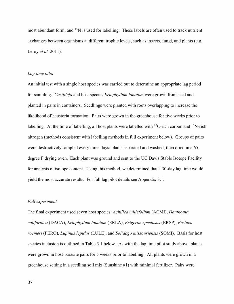
37

most abundant form, and 15N is used for labelling. These labels are often used to track nutrient

exchanges between organisms at different trophic levels, such as insects, fungi, and plants (e.g.

Leroy et al. 2011).

Lag time pilot

An initial test with a single host species was carried out to determine an appropriate lag period

for sampling. Castilleja and host species Eriophyllum lanatum were grown from seed and

planted in pairs in containers. Seedlings were planted with roots overlapping to increase the

likelihood of haustoria formation. Pairs were grown in the greenhouse for five weeks prior to

labelling. At the time of labelling, all host plants were labelled with 13C-rich carbon and 15N-rich

nitrogen (methods consistent with labelling methods in full experiment below). Groups of pairs

were destructively sampled every three days: plants separated and washed, then dried in a 65-

degree F drying oven. Each plant was ground and sent to the UC Davis Stable Isotope Facility

for analysis of isotope content. Using this method, we determined that a 30-day lag time would

yield the most accurate results. For full lag pilot details see Appendix 3.1.

Full experiment

The final experiment used seven host species: Achillea millefolium (ACMI), Danthonia

californica (DACA), Eriophyllum lanatum (ERLA), Erigeron speciosus (ERSP), Festuca

roemeri (FERO), Lupinus lepidus (LULE), and Solidago missouriensis (SOMI). Basis for host

species inclusion is outlined in Table 3.1 below. As with the lag time pilot study above, plants

were grown in host-parasite pairs for 5 weeks prior to labelling. All plants were grown in a

greenhouse setting in a seedling soil mix (Sunshine #1) with minimal fertilizer. Pairs were

38

grown in greenhouse plug trays and watered regularly to ensure survival. Each host-parasite pair

was replicated 26 times. Some mortality occurred during the experiment, and the lowest final

treatment group size was 18 host-parasite pairs.

Table 3.1 Host species used in companion plantings. Basis for inclusion key: 1 - known host of

C. levisecta; 2 - genus parasitized by other Castilleja species; 3 - observed near robust C.

levisecta in field).

Species Family Functional

Group

Basis for

inclusion

Achillea millefolium Asteraceae Forb 1

Danthonia californica Poaceae Grass 1

Erigeron speciosus Asteraceae Forb 1

Eriophyllum lanatum Asteraceae Forb 1,3

Festuca roemeri Poaceae Grass 1

Lupinus lepidus Fabaceae Legume 1,2

Solidago canadensis Asteraceae Forb 1

Isotope labelling

Carbon was added via 13CO2 (purchased from Sigma-Aldrich) injected into bags covering host

plants as in Philip & Simard (2008), (see Figure 3.1). Injected bags were left on host plants for a

five-hour pulse period, then removed in a windy environment to avoid contamination.

Nitrogen was added by immersing cut leaves of the host plant in a 30 mM ammonium sulfate

((15NH4)2SO4) solution (purchased from Sigma-Aldrich) as in Aflakpui et al. (2005), (see Figure

3.1). Leaves were left in the emersion for 24 hours, after which the solution was removed. All

pairs were given a thirty-day lag period before sampling to allow transfer from host to parasite.

Once the lag period ended, host and parasite were separated, rinsed, and dried. Whole plant

Castilleja individuals were then ground to powder and a sample (1.0 - 2.5 mg) of each sent out

for testing.

39

Samples were sent to the UC Davis Isotope Lab for analysis. Data were returned as δ (del)

values of carbon and nitrogen. Del is defined by the following equation, where R is the ratio of

the heavy to the light isotope, and the standard is an accepted, known substance used for

comparison:

Del value (in permil) = (Rsample/Rstandard – 1) * 1000

The standards used for comparison were VPDB (Vienna Pee Dee Belemnite) for carbon and air

for nitrogen.

40

Analysis

Values of each host group were compared for del 13C and del 15N using a Kruskal-Wallis test

(alpha = 0.05) in R statistical software (version 3.2.2, Appendix B). This test was used because

the data did not fit the assumptions of normal distribution needed for an ANOVA test. Pairwise

comparisons were then made between each treatment group to determine specific differences in

host-derived nutrition using a post-hoc Nemenyi test (alpha = 0.05). We also compared the del

values of carbon and nitrogen within host treatments and overall in the study.

Results

Outcomes from the Kruskal-Wallis test are shown in Table 3.2 below. Both carbon and nitrogen

analyses had significant results.

Table 3.2 Chi-squared, degrees of freedom, and p-values for Kruskal-Wallis tests of host identity

as a predictor of del values of 13C and 15N in Castilleja.

Chi-squared df p-value

Carbon 51.112 6 p < 0.00001

Nitrogen 57.164 6 p < 0.00001

Carbon

Host identity was a significant predictor of del 13C (Table 3.2). Some host groups differed in the

amount of labelled carbon found in the paired Castilleja (Figure 3.2). Solidago was the highest

performing host group, with the highest del 13C value (the highest portion of Castilleja biomass

was host-derived). This group differed significantly from all other treatment groups. All other

41

host groups were similar to each other, with the exception of the lowest performing group:

Erigeron.

Nitrogen

Host identity was also a significant predictor of del 15N (Table 3.2). As with carbon, many groups’

del 15N values were significantly different from others, and a wide range of values was seen

among the groups (Figure 3.3). Highest values were present in those Castilleja parasitizing

Eriophyllum, and Achillea, while the lowest value was seen in the Erigeron treatment group.

42

Discussion

Carbon

Globally (excluding dry climates) most C3 plants’ del 13C values range between 28 and 32

(Kohn 2010). Based on this, there did not appear to be large quantities of host-derived carbon

present in Castilleja overall (Figure 3.2). There are two likely reasons for this. The first is that

the actual product acquired from the host (xylem sap) does not contain large quantities of carbon

to begin with. If this is the case, the parasite would need to obtain large quantities of xylem sap

in order to get significant amounts of carbon from its host. Looking at our lag pilot data (Figure

43

S3.2), the del 13C in Castilleja peaks at a far lower value than the host plant. This indicates that,

while there may be some quantity of carbon acquisition from hosts, Castilleja does not seem to

gain large amounts of carbon from host plants. The second possible reason is that there is not a

great enough need, and thus not a large enough “pull” from the parasite for carbon. Since

Castilleja is a hemiparasite and can sequester its own carbon, it does not rely on its host for a

significant portion of its overall carbon. Our test environment was well-lit (greenhouse) and all

plants were early enough in their life cycles that they did not compete with each other for light.

Had we used older pairs in which hosts shaded out the parasites, perhaps we would have seen

greater amounts of host-derived carbon in the parasites. Studies on hemiparasites in the same

family (Orobanchaceae) found that shading increased the proportion of parasite biomass that was

host-derived (Tesitel et al. 2011).

Nitrogen

Nitrogen acquisition differed greatly between host treatments (Figure 3.3). The standard used for

15N comparison is atmospheric nitrogen (del = 0), and due to low levels of nitrogen isotope

discrimination by plants, the expectation is that base (unlabeled) del 15N values are near zero

(Evans and Ehleringer 1994). Compared to this baseline, all treatments in our study showed high

levels of host-derived nitrogen in the parasites. Earlier studies have shown Eriophyllum to be a

good host for this parasite (Delvin 2013), and the nitrogen input shown in Figure 3.3 may point

to a mechanism. Pacific Northwest prairie remnants are often found in nitrogen-limited soils

(Dunwiddie and Bakker 2011), so additional inputs of host nitrogen could have great benefits to

the parasite. An additional note is the high level of nitrogen gained from the host Achillea.

44

Additional studies in this lab (Schmidt, unpub. data) have found Achillea to be a highly suitable

host for this species, and greater inputs of nitrogen could lead to this advantage.

Care should be taken with interpretation of 15N input from the Lupinus species. The measured

level of nitrogen input does not include additional nitrogen gained from bacteria-mediated

atmospheric N-fixation, which would not have been labelled using our methods. With this in

mind, we are unable to fully estimate the true amount of nitrogen being sequestered by Castilleja

parasitizing lupine hosts. The additional nitrogen supplied by this host could increase Castilleja’s

competitive ability and allow it greater access to sunlight by means of increased height.

Study limitations

One caveat to this study is the possibility that the results could have been skewed due to the lag

time and isotope labelling methodologies applied. The pilot study to determine lag time utilized

a single host species (Eriophyllum), while the full experiment employed multiple host species

with varying leaf sizes. This may be important for the nitrogen isotope results, as cut leaves were

the method of application of the labelled compound (see methods). While an attempt was made

during labelling to ensure an adequate area of tissue was cut on each species, it was difficult to

cut large areas of grass leaves, especially those as thin as Festuca. It is yet unclear whether this

significantly affected our results (by differential host uptake of carbon or nitrogen), but should be

addressed in future experiments of this nature. It is also possible that some degree of host benefit

was related to host species’ root structure or number of haustorial connection, which were not

categorized in this study.

45

Implications

This study points to mechanisms behind host preference by parasites and differential parasite

performance related to host species. For Castilleja levisecta specifically, there are implications

for management due to its status as a threatened species. In sites where competition with taller-

statured species is likely, C. levisecta may have less access to sunlight and thus become carbon

limited. In this case land managers may wish to seed or plant C. levisecta with Solidago

missouriensis to increase heterotrophic carbon acquisition opportunities for the parasite.

Similarly, if soil is nitrogen-limited, it may be prudent to plant or seed with Eriophyllum

lanatum. Some parasitic plants have shown improved performance with mixed-host diets

(Marvier 1998), so an optimal host regime may even be a mix of S. missouriensis and E.

lanatum.

On a broader scale, this research adds to the growing body of knowledge investigating the

mechanisms of host selectivity in parasitic angiosperms. It adds to the conclusions of Demey

and colleagues’ 2015 study showing differential performance of two other hemiparasites

(Rhinanthus and Pedicularis) based on host identity. Their study showed differences within

rather than among host functional groups, aligning with our host-derived nutrition results. Rather

than relying on the broad categorization of functional groups to define host quality, we need to

investigate at a finer scale to identify optimal host species. With this as a platform, we can

continue to investigate the intricacies of host-parasite relationships.

46

Conclusions

This study sheds light on the mechanisms behind host suitability to parasitic plants and the role

that nutrition plays in these relationships. Future studies may seek to elucidate the precise fate of

host-derived nutrients in parasites (leaves, stems, roots), or to track additional host-derived

resources such as water or specific defensive compounds. Gaps in knowledge are also present in

the study of this mechanism on additional parasitic angiosperms. It is our hope that

experimentation in this line of inquiry continues for both widespread and rare or endangered

parasitic angiosperms.

47

References

Adler, L.S. 2003. Host species affects herbivory, pollination, and reproduction in experiments

with parasitic Castilleja. Ecology, 84(8): 2083–2091.

Aflakpui, G.K.S., P.J. Gregory, and R.J. Froud-Williams. 2005. Carbon (13C) and Nitrogen

(15N) translocation in a Maize-Striga hermonthica association. Experimental Agriculture, 41(3):

321-333.

Ducharme, L.A. and J.R. Ehlringer. 1996. Gas exchange, delta C-13, and hetertrophy for

Castilleja linariifolia and Orthocarpus tolmiei, facultative root hemiparasites on Artemisia

tridentata. Great Basin Naturalist, 56(4): 333-340.

Dunwiddie, P., and J.D. Bakker. 2011. The Future of Restoration and Management of Prairie-

Oak Ecosystems in the Pacific Northwest. Northwest Science 85: 83–92.

Delvin, E. 2013. Restoring Abandoned Agricultural Lands in Puget Lowland Prairies: A New

Approach. PhD Thesis, University of Washington. Seattle, WA.

Demey, A., P. De Frenne, L. Baeten, G. Verstraeten, M. Hermy, P. Boeckx, and K. Verheyen.

2015. The effects of hemiparasitic plant removal on community structure and seedling

establishment in semi-natural grasslands. Journal of Vegetation Science, 26(3): 409-420.

Evans, R.D., and J.R. Ehleringer. Plant δ15N values along a fog gradient in the Atacama Desert,

Chile. Journal of Arid Environments, 28(3): 189-193.

Kohn, M.J. 2010. Carbon isotope compositions of terrestrial C3 plants as indicators of

(paleo)ecology and (paleo)climate. Proceedings of the National Academy of Sciences of the

United States of America, 107(46): 19691-19695.

Leroy, C., N. Sejalon-Delmas, A. Jauneau, M.X. Ruiz-Gonzales, H. Gryta, P. Jargeat, B.

Corbara, A. Dejean, and J. Orivel. 2011. Trophic mediation by a fungus in an ant-plant

mutualism. Journal of Ecology, 99(2): 583-590.

Li, A.R., Y.J. Li, S.E. Smith, F.A. Smith, and K.Y. Guan. 2013. Nutrient requirements differ in

two Pedicularis species in the absence of a host plant: implication for driving forces in the

evolution of host preference of root hemiparasitic plants. Annals of Botany, 112(6): 1099-1106.

Marko, M.D. and F.R. Stermitz. 1997. Transfer of alkaloids from Delphinium to Castilleja via

root parasitism. Norditerpenoid alkaloid analysis by electrospray mass spectrometry.

Biochemical Systematics and Ecology, 25(4): 279-285.

Marshall, J.D., J.R. Ehleringer, E.D. Schulze, and G.D. Farquhar. 1994. Carbon isotope

composition, gas exchange and heterotrophy in Australian mistletoes. Functional Ecology, 8:

237-241.

48

Marshall, J.D. and J.R. Ehleringer. 1990. Are xylem tapping mistletoes partially heterotrophic?

Oecologia, 84: 244-248.

Marvier, M. 1998. A mixed diet improves performance and herbivore resistance of a parasitic

plant. Ecology, 79(4): 1272-1280.

Pate, J.S., K.C. True, and E. Rasins. 1991. Xylem transport and storage of amino acids by S. W.

Australian mistletoes and their hosts. Journal of Experimental Botany, 42: 441-451.

Philip, L.J. and S.W. Simard. 2008. Minimum pulses of stable and radioactive carbon isotopes to

detect belowground carbon transfer between plants. Plant Soil, 308 (1-2): 23-25.

Schulze, E.D., O.L. Lange, H. Zeigler, and G. Gebaur. 1991. Carbon and nitrogen isotope ratios

of mistletoes growing on nitrogen and non nitrogen fixing hosts and on CAM plants in the

Namib desert confirm partial heterotrophy. Oecologia, 88: 457-462.

Stermitz, F.R. and G.H. Harris. 1987. Transfer of pyrrolizidine and quinolizidine alkaloids to

Castilleja (Scrophulariaceae) hemiparasites from composite and legume host plants. Journal of

Chemical Ecology, 13(8): 1917-1925.

Tesitel, J., T. Tesitelova, J.P. Fisher, J. Leps, and D.D. Cameron. 2015. Integrating ecology and

physiology of root-hemiparasitic interaction: interactive effects of abiotic resources shape the

interplay between parasitism and autotrophy. New Phytologist, 205(1): 350-360.

Tesitel, J., J. Leps, M. Vrablova, and D.D. Cameron. 2011. The role of heterotrophic carbon

acquisition by the hemiparasitic plant Rhinanthus alectorophus in seedling establishment in

natural communities: a physiological perspective. New Phytologist, 192(1): 188-199.

Tesitel, J., L. Plavcova, and D.D. Cameron. 2010. Heterotrophic carbon gain by the root

hemiparasites, Rhinanthus minor and Euphrasia rostkoviana (Orobanchaceae). Planta, 231(5):

1137-114.

49

Appendix 3.1: Lag time pilot experiment

Timing of parasitic nutrient uptake can vary between species and within species at different life

stages. In the study above we looked into the nutrient transfer of many host species to a specific

parasite: Castilleja levisecta. In order to prepare to test this transfer using multiple host species

for Castilleja levisecta, we first needed to determine an appropriate lag time (time between

isotope labelling of hosts and sampling of Castilleja).

An initial test with a single host species was carried out to determine an appropriate lag period

for sampling. Castilleja and host species Eriophyllum lanatum were grown from seed and

planted in pairs in containers. Seedlings were planted with roots overlapping to increase the

likelihood of haustorium formation. Pairs were grown in the greenhouse for five weeks prior to

labelling. At the time of labelling, all host plants were labelled with 13C-rich carbon and 15N-rich

nitrogen.

Carbon was added via 13CO2 injected into bags covering host plants as in Philip & Simard

(2008). Injected bags were left on host plants for a five-hour pulse period, then removed in a

windy environment to avoid contamination. Nitrogen was added by immersing cut leaves of the

host plant in a 30 mM ammonium sulfate solution ((15NH4)2SO4) as in Aflakpui et al. (2005).

Leaves were left in the emersion for 24 hours, then the solution was removed.

Groups of pairs were destructively sampled every three days: plants separated and washed, then

dried in a 65-degree F drying oven. Each plant was ground to powder and sent to the UC Davis

Stable Isotope Facility for analysis of isotope content. Data was returned as δ (del) values of

50

carbon and nitrogen. Del is defined by the following equation, where R is the ratio of the heavy

to the light isotope, and the standard is an accepted, known substance used for comparison:

Del value (in permil) = (Rsample/Rstandard – 1) * 1000

Del 15N values of the host plants decrease over time as Castilleja’s values increase (Figure S3.1).

There is an early bump in host del 13C values followed by a smaller bump in Castilleja’s values

around 12 days following labelling (Figure S3.2). However, after this initial bump the values of

del 13C in Castilleja continue to fluctuate. The scale in each of the graphs should also be noted,

such that despite the seemingly smaller slope in the rise of Castilleja’s del 15N, there is a much

greater increase in labelled nitrogen over time than there is carbon. This in itself is somewhat

expected due to Castilleja’s status as a hemiparasite: it is able to photosynthesize and sequester

carbon without the aid of a host. This fact coupled with the full sun conditions of the experiment

perhaps led to less need for host-derived carbon in this setting.

Based on the steady increase in del 15N of Castilleja through the duration of the pilot and

despite the minor uptick in del 13C around the midpoint of the experiment, we chose to use the

longest tested lag time, 30 days, for the full experiment. The nitrogen transfer appeared to be the

stronger signal to indicate the highest level of xylem sap transfer.

51

Figure S3.1 Del 15N values of Castilleja (CALE) and host species in days following label

addition to host plant.

Figure S3.2 Del 13C values of Castilleja (CALE) and host species in days following label

addition to host plant.

0

5000

10000

15000

20000

25000

0 5 10 15 20 25 30 35

Del

15N

Days after label

CALE

Host

-50

0

50

100

150

200

250

0 5 10 15 20 25

Del

13C

Days after label

CALE

Host

52

Chapter 4: Do all parasitic plants work as ecosystem engineers? A case study in Pacific

Northwest prairies

Abstract

Parasitic plants inhabit a unique niche in their native ecosystems, which some ecologists argue

makes them ecosystem engineers. Several case studies have shown parasitic plants affect the

composition of the communities they inhabit. We examined this effect at varying spatial and

temporal scales using Pacific Northwest prairies as a test system, and hemiparasitic Castilleja as

our ecosystem engineer. Unlike previous studies, we find conflicting evidence for this

community effect, whether due to a weak signal or masking by other community change factors

such as local weather. Our results suggest that examining this type of ecosystem effect on a

larger spatial and temporal scale may add nuance to our understanding of parasitic plants’ roles

in their native systems, and that parasites may not always have a strong effect.

Introduction

Parasitic angiosperms have long been studied for their negative effects on crop species and

silviculture (e.g. Spallek et al. 2013). Striga (witchweed) and Arceuthobium (dwarf mistletoes)

are two examples of heavily studied parasites. Striga parasitizes food crops such as corn

(Mumera and Below 1993), and dwarf mistletoes grow on and parasitize large trees such as

Pinus (Stanton 2006). Much of our initial knowledge of mechanisms of parasitism was gleaned

from the study of these devastating parasites.

More recently, scientists have begun investigating the potential for positive effects of parasites

on their native systems. These positive impacts range from facilitation of greater species

richness (Bao et al. 2015) to increased nitrogen transformation in soil (Demey et al. 2014).

53

Several studies show that parasitic angiosperms may play an important role in community

assembly and composition (Pywell et al. 2004, Grewell 2008, Decleer et al. 2013). There are

many species which may facilitate nutrient cycling in their native ecosystems by acquiring

nutrients from their host(s) and redistributing them through nutrient-rich litter (Quested et al.

2005, Press 1998). Hemiparasitic Orobanchaceae are also thought to alter competition between

hosts and non-hosts, thus causing changes in community composition (Phoenix and Press 2005).

In some cases, the parasite’s negative impact on host biomass may sometimes be outweighed by

their positive impact on the total plant community biomass (Fisher et al. 2013).

In Europe, the addition of hemiparasitic Rhinanthus species into degraded landscapes has been

used in grassland restoration to increase species richness and diversity (Pywell et al. 2004,

Westbury et al. 2004, Bullock and Pywell 2005). Overall, studies are beginning to show that

parasitic plants can have significant direct and indirect effects on the surrounding plant

community (Watson 2009).

In a recent study, Bao et al. (2015) showed an increase in species richness on plots with

hemiparasite Pedicularis kansuensis present. Their study used a degraded grassland site in the

Qinghai-Tibet Plateau and set up plots with and without P. kansuensis through removal of the

parasite from control sites. After one year of this treatment, they measured species richness in

each plot and found greater richness in those plots with the parasite present.

We examined this effect to determine the variability it shows over various spatial and temporal

scales. Our objective was to answer the following questions:

54

1. Is there an effect of parasites on plant community similar to recent findings present in an

untested system?

2. Is this effect consistent at all sites in all years?

3. If present, does this effect grow stronger or weaker over time?

Methods

Study species and site

Castilleja levisecta Greenm. and C. hispida Benth. are short-lived perennials native to the

prairies of the Pacific Northwest. Both species are facultative hemiparasites: they procure

resources from other host plants but they are able to survive and reproduce without a host

present, and they have the ability to sequester carbon via photosynthesis. These species, as with

all plants in the genus Castilleja, attach to their hosts using parasitic root structures, called

haustoria, which facilitate a xylem-xylem connection between the parasite and its host (Kuijt

1969). Both species have small, nondescript flowers covered by showy bracts; C. levisecta’s are

a bright yellow and C. hispida most often red-orange but occasionally yellow.

The prairies of the Pacific Northwest represent a unique ecosystem: they were historically

maintained with intentional burning for centuries by native peoples (Boyd 1999) and are home to

a variety of rare and endangered species (Altman 2011, Fazzino et al. 2011, Schultz et al. 2011,

Stinson 2005). Since European settlement, these ecosystems have declined from covering over

73,000 ha to fewer than 7,000 ha, due in large part to fire suppression, development, and

agriculture (Franklin and Dyrness 1988, Crawford and Hall 1997, Dunwiddie 2002).

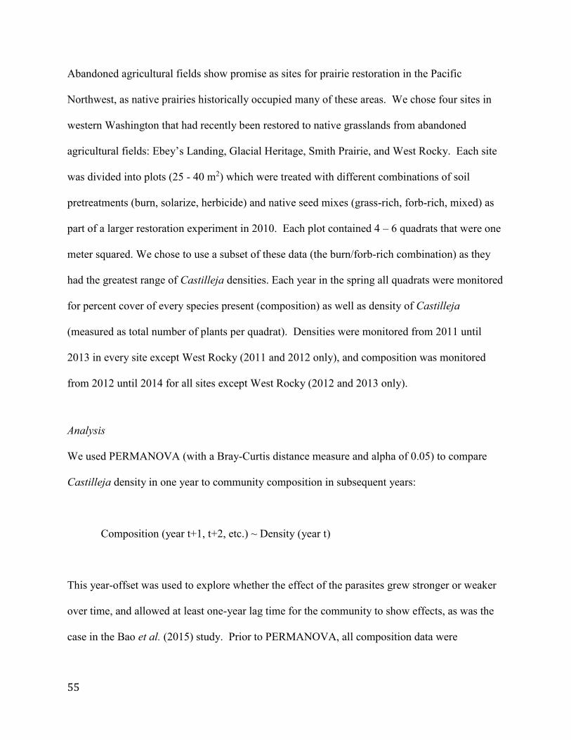
55

Abandoned agricultural fields show promise as sites for prairie restoration in the Pacific

Northwest, as native prairies historically occupied many of these areas. We chose four sites in

western Washington that had recently been restored to native grasslands from abandoned

agricultural fields: Ebey’s Landing, Glacial Heritage, Smith Prairie, and West Rocky. Each site

was divided into plots (25 - 40 m2) which were treated with different combinations of soil

pretreatments (burn, solarize, herbicide) and native seed mixes (grass-rich, forb-rich, mixed) as

part of a larger restoration experiment in 2010. Each plot contained 4 – 6 quadrats that were one

meter squared. We chose to use a subset of these data (the burn/forb-rich combination) as they

had the greatest range of Castilleja densities. Each year in the spring all quadrats were monitored

for percent cover of every species present (composition) as well as density of Castilleja

(measured as total number of plants per quadrat). Densities were monitored from 2011 until

2013 in every site except West Rocky (2011 and 2012 only), and composition was monitored

from 2012 until 2014 for all sites except West Rocky (2012 and 2013 only).

Analysis

We used PERMANOVA (with a Bray-Curtis distance measure and alpha of 0.05) to compare

Castilleja density in one year to community composition in subsequent years:

Composition (year t+1, t+2, etc.) ~ Density (year t)

This year-offset was used to explore whether the effect of the parasites grew stronger or weaker

over time, and allowed at least one-year lag time for the community to show effects, as was the

case in the Bao et al. (2015) study. Prior to PERMANOVA, all composition data were

56

transformed using the “wisconsin” function, in which species are first standardized by maxima

and then sites by site totals (Oksanen et al. 2015).

Following PERMANOVA, ordisurf plots were created to visualize differences in community

composition based on Castilleja density. Ordisurf plots (from the “vegan” statistics package)

show the similarity between plots using multivariate community composition data represented in

two dimensions overlaid with Castilleja density at each plot (NMDS). These plots were

obtained using a Bray-Curtis distance measure. The position of the bubbles represents the

similarity or difference in community data between plots and the size of the bubbles shows the

relative density of Castilleja at each plot. The lines are a fitted contour of Castilleja densities.

Using this function, we create a visual representation of the similarities between plant

communities in addition to Castilleja density data from which we may be able to see a pattern.

We additionally used PERMANOVA (with an Euclidean distance measure, alpha = 0.05) to test

species richness in a similar manner:

Richness (year t+1, t+2, etc.) ~ Density (year t)

57

This provided a total of six analyses per site (except West Rocky):

2011 density x 2012 composition/richness

2011 density x 2013 composition/richness

2011 density x 2014 composition/richness

2012 density x 2013 composition/richness

2012 density x 2014 composition/richness

2013 density x 2014 composition/richness

These tests were replicated with each community measure (multivariate community composition

or species richness), for a total of 12 separate analyses per site.

We also visually analyzed the possible time lag effect of Castilleja influence by graphing the

number of years between measurements (e.g. Castilleja density measured in 2011 and species

richness in 2014 = 3-year difference) and the associated proportion of variation explained by

Castilleja density. This helped us to explore the possibility of Castilleja’s impact growing

stronger or weaker over time. Similarly, we visually represented the median density in each

analysis compared to the R2 value for that PERMANOVA. We used this method to examine the

possibility that the signal of parasites’ effect on the community was more visible on sites with

greater ranges of Castilleja densities. The purpose of these multiple analyses was to ensure that if

there were community changes due to parasite abundance, they were found and included in the

study. Analyses were conducted using R statistical software (version 3.1.3, Appendix C).

58

Results

Community composition

PERMANOVA results comparing Castilleja density to community composition were variable

between different sites and different combinations of years (Table 4.1). Castilleja density had a

significant effect on composition in all combinations of years at the Ebey’s Landing site, but

only two combinations of years at Glacial Heritage and none of the combinations at the other two

sites. At Glacial Heritage the 2011 Castilleja density did not show a significant effect on

community until three years later, but the 2012 density only had a significant effect the following

year.

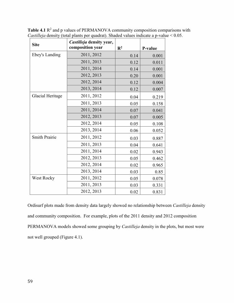
59

Table 4.1 R2 and p values of PERMANOVA community composition comparisons with

Castilleja density (total plants per quadrat). Shaded values indicate a p-value < 0.05.

Site Castilleja density year,

composition year R2 P-value

Ebey's Landing 2011, 2012 0.14 0.001

2011, 2013 0.12 0.011

2011, 2014 0.14 0.001

2012, 2013 0.20 0.001

2012, 2014 0.12 0.004

2013, 2014 0.12 0.007

Glacial Heritage 2011, 2012 0.04 0.219

2011, 2013 0.05 0.158

2011, 2014 0.07 0.041

2012, 2013 0.07 0.005

2012, 2014 0.05 0.108

2013, 2014 0.06 0.052

Smith Prairie 2011, 2012 0.03 0.887

2011, 2013 0.04 0.641

2011, 2014 0.02 0.943

2012, 2013 0.05 0.462

2012, 2014 0.02 0.965

2013, 2014 0.03 0.85

West Rocky 2011, 2012 0.05 0.078

2011, 2013 0.03 0.331

2012, 2013 0.02 0.831

Ordisurf plots made from density data largely showed no relationship between Castilleja density

and community composition. For example, plots of the 2011 density and 2012 composition

PERMANOVA models showed some grouping by Castilleja density in the plots, but most were

not well grouped (Figure 4.1).

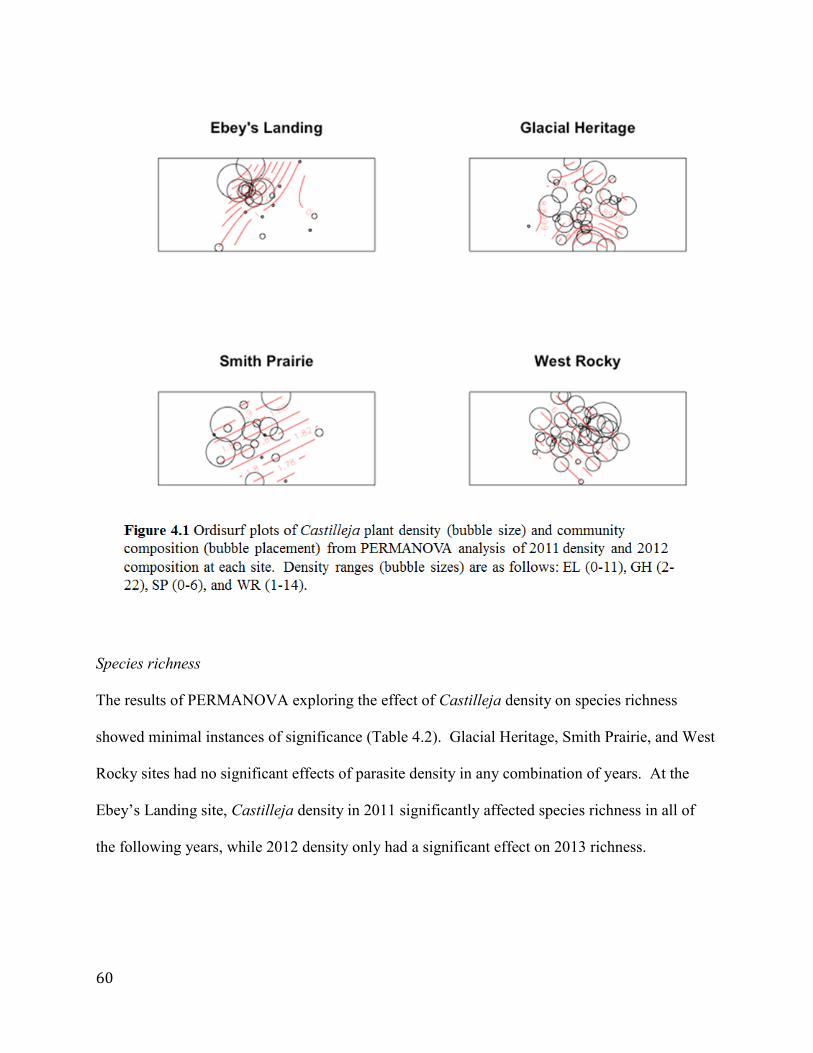
60

Species richness

The results of PERMANOVA exploring the effect of Castilleja density on species richness

showed minimal instances of significance (Table 4.2). Glacial Heritage, Smith Prairie, and West

Rocky sites had no significant effects of parasite density in any combination of years. At the

Ebey’s Landing site, Castilleja density in 2011 significantly affected species richness in all of

the following years, while 2012 density only had a significant effect on 2013 richness.

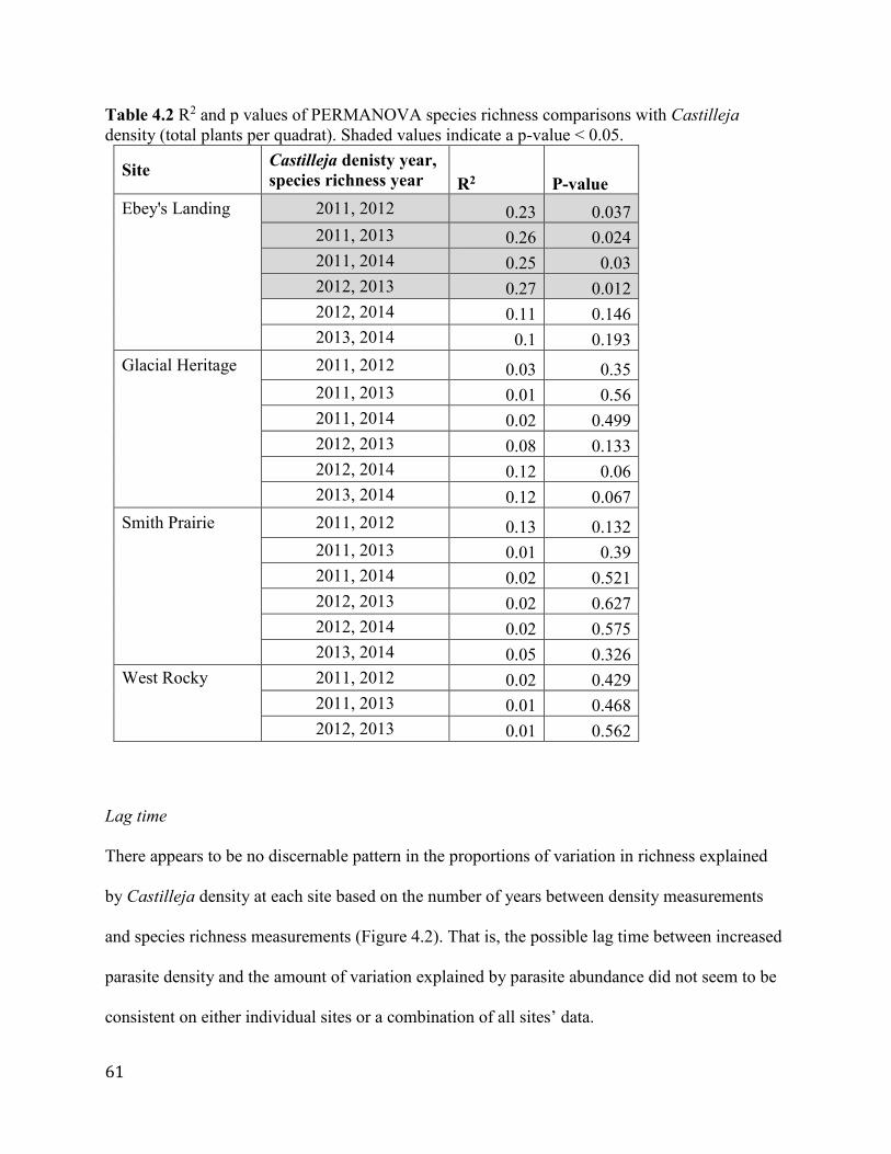
61

Table 4.2 R2 and p values of PERMANOVA species richness comparisons with Castilleja

density (total plants per quadrat). Shaded values indicate a p-value < 0.05.

Site Castilleja denisty year,

species richness year R2 P-value

Ebey's Landing 2011, 2012 0.23 0.037

2011, 2013 0.26 0.024

2011, 2014 0.25 0.03

2012, 2013 0.27 0.012

2012, 2014 0.11 0.146

2013, 2014 0.1 0.193

Glacial Heritage 2011, 2012 0.03 0.35

2011, 2013 0.01 0.56

2011, 2014 0.02 0.499

2012, 2013 0.08 0.133

2012, 2014 0.12 0.06

2013, 2014 0.12 0.067

Smith Prairie 2011, 2012 0.13 0.132

2011, 2013 0.01 0.39

2011, 2014 0.02 0.521

2012, 2013 0.02 0.627

2012, 2014 0.02 0.575

2013, 2014 0.05 0.326

West Rocky 2011, 2012 0.02 0.429

2011, 2013 0.01 0.468

2012, 2013 0.01 0.562

Lag time

There appears to be no discernable pattern in the proportions of variation in richness explained

by Castilleja density at each site based on the number of years between density measurements

and species richness measurements (Figure 4.2). That is, the possible lag time between increased

parasite density and the amount of variation explained by parasite abundance did not seem to be

consistent on either individual sites or a combination of all sites’ data.

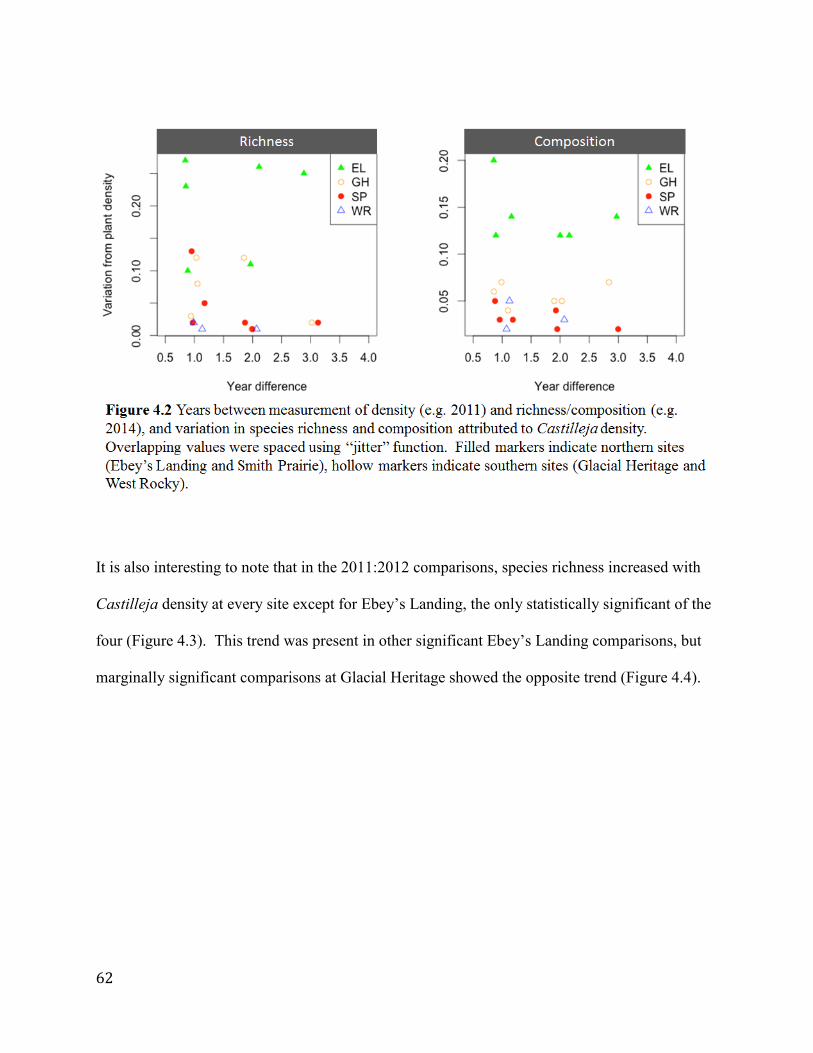
62

It is also interesting to note that in the 2011:2012 comparisons, species richness increased with

Castilleja density at every site except for Ebey’s Landing, the only statistically significant of the

four (Figure 4.3). This trend was present in other significant Ebey’s Landing comparisons, but

marginally significant comparisons at Glacial Heritage showed the opposite trend (Figure 4.4).

63

64

Discussion

While a single site had significant results of parasite density effects on community composition

and richness, the majority of our site and year combinations were not significant. The one other

site that showed significant results had inconsistency in lag time. Our results did not indicate a

clear lag time present throughout the sites, although the data from Ebey’s Landing suggests that

in some cases the effect of a parasite on the community can be present for several years. The

overall results indicate two possibilities:

65

1) The effect of parasites on composition and richness in this system varies spatially and

temporally

2) There are significant effects of parasites on most sites but they are sometimes masked by

other factors

Changes in significance by year and site may be due to actual significance of this effect being

outweighed by other factors such as weather, herbivory, or another site-specific variable. While

the sites chosen were paired in geographic location, there were still potential differences in

microclimate at each site in each year. This may have been one cause of the stochastic results

we observed. Additionally, other factors such as herbivory may have varied site to site.

Differences in initial site conditions may also play a role in these inconsistencies. Although all

sites used in this study were abandoned agricultural fields, they varied in their usage history and

previous crops on site. While we endeavored to use site pretreatments to ensure as much

uniformity as possible among sites, it is possible that historical usage still had an effect on our

results. In the South Sound sites, Glacial Heritage soils are categorized as Nisqually loamy fine

sand, while West Rocky soils are Spanaway-Nisqually complex (NRCS online database).

Nisqually loamy fine sand soils in the area are mostly used for agricultural production, while the

Spanaway-Nisqually complex is present at many of the poorer prairie sites left as remnants. In

the North Sound, soil at both sites is characterized as San Juan sandy loam, but Smith Prairie’s

soil has more gravel and holds less moisture than Ebey’s Landing (Delvin 2013). In addition,

Castilleja levisecta is known to be more successful in soils that are deeper and more productive

(Dunwiddie et al. 2016, Delvin 2013).

66

The range of variation of the actual parasite densities (summarized in Figure S4.1) may also have

influenced our results. It should be noted that while Glacial Heritage has the highest median

density values, it does not always show the greatest R2 values to match, and in the case of

community composition it is the lower of the median densities from that site which show the

greatest R2 (Tables 4.1 and 4.2).

Despite this variability and potential for site-specific differences, it seems that in several cases

there is an effect of parasitic plant density on community composition and richness. Two

mechanisms have been suggested for this effect.

The first is an alteration of nutrient cycling by parasites. When nutrients are obtained from the

host plant, they are incorporated into parasite tissues, including parasite leaves. When leaves are

dropped in summer, this nutrient-rich litter becomes incorporated into the soil and the nutrients

become available to other plants (Fisher et al. 2013). By this mechanism, nutrients originating in

host species tissues can be redistributed to soil and from there to non-host plants in the

community.

The second mechanism is through host suppression. As parasites take nutrients from their hosts,

hosts become less able to grow and thrive, thus reducing their competitive ability in relation to

non-host species. In cases where host species are dominant or abundant in the plant community

this can cause significant reduction in plant biomass overall, while also potentially increasing

species richness (Demey et al. 2015). In our study, Castilleja density had negative or non-

significant effects on species richness, depending on the site and year (e.g. Figures 4.3 and 4.4),

67

although two marginally significant effects had a positive effect (see Glacial Heritage in Table

4.2, Figure 4.4).

It should be noted that our comparisons with other studies are not direct, since we used the range

of parasite density already present in place of a parasite removal for comparison (as in Bao et al.

2016 and Demey et al. 2015). In removal experiments it is possible that removal plots retain the

effect of the parasites following removal for some period of time, which has the potential to

skew results. Our method provides a natural gradient of variation in parasite density, but does

not look at the direct comparison of communities with none and with an abundance of parasites.

Despite the mixed results indicating parasite effects on the plant community, the several

significant results lead us to believe that this effect does exist in this system. However, it may

not be as strong as that shown in Bao 2015. As we begin to study ecosystems over larger spatial

and temporal scales, (as in Grace et al. 2016), our understanding of more general ecological

patterns is improved.

Conclusions

To answer our original research questions, 1) We did in some cases find an effect of parasites on

plant communities, but not in a majority of our samples. Overall our results were dissimilar to

the Bao 2015 study. 2) The effect was not consistent across sites or years, and there was much

inconsistency among sites concerning which years had significant results. 3) The effect did not

seem to have a pattern of strengthening or weakening over time. Results seemed more stochastic

among different years and did not appear to be linked to a specific lag time.

68

While our data did not conclusively support the case for community changes due to parasitism

across the board, they do point to the need for further research in this area. Studies that explore

this effect over larger spatial and temporal scales may shed more light on the nuances of these

parasite-community interactions. For example, if we had used only the Ebey’s Landing or a

single year’s data in our study, we may have come to different conclusions. Larger and longer

studies are needed to more fully understand the complexities of the relationship between

parasitic plants and their communities.

69

References

Altman, B. 2011. Historical and Current Distribution and Populations of Bird Species in Prairie-

Oak Habitats in the Pacific Northwest. Northwest Science, 85:194–222.

Bao, G.S., K. Suetsugu, H.S. Wang, X. Yao, L. Liu, J. Ou, and C.J. Li. 2015. Effects of the

hemiparasitic plant Pedicularis kansuensis on plant community structure in a degraded

grassland. Ecological Research, 30(3): 507-515.

Boyd, R. 1999. Indians, Fire, and the Land in the Pacific Northwest. Page 320. Oregon State

University Press, Corvallis, OR.

Bullock, J.M and R.F. Pywell. 2005. Rhinanthus: A tool for restoring diverse grasslands?. Folia

Geobotanica, 40(2-3): 273-288.

Crawford, R. C., and H. Hall. 1997. Changes in the South Puget Sound Prairie Landscape. Pgs

11–16. Ecology and Conservation of the South Puget Sound Prairie Landscape. P.W.

Dunnwiddie and K. Ewing eds. The Nature Conservancy. Seattle, WA.

Decleer, K., D. Bonte, and R. Van Diggelen. 2013. The hemiparasite Pedicularis palustris:

‘Ecosystem engineer’ for fen-meadow restoration. Journal for Nature Conservation, 21(2): 65-

71.

Demey, A., P. De Frenne, L. Baeten, G. Verstraeten, M. Hermy, P. Boeckx, and K. Verheyen.

2015. The effects of hemiparasitic plant removal on community structure and seedling

establishment in semi-natural grasslands. Journal of Vegetation Science, 26(3): 409-420.

Demey, A., T. Rutting, D. Huygens, J. Staelens, M. Hermy, K. Verheyen, and P. Boeckx. 2014.

Hemiparasitic litter additions alter gross nitrogen turnover in temperate semi-natural grassland

soils. Soil Biology and Biochemistry, 68: 419-428.

Dunwiddie, P.W. 2002. Management and restoration of grasslands on Yellow Island,

San Juan Islands, Washington, USA. Pgs 78-87. Garry Oak Ecosystem Restoration: Progress and

Prognosis. Proceedings of the Third Annual Meeting of the B.C. Chapter of the Society for

Ecological Restoration, April 27-28, 2002, P. J. Burton ed. University of Victoria. B.C. Chapter

of the Society for Ecological Restoration, Victoria, British Columbia.

Dunwiddie, P.W., N.L. Haan, M. Linders, J.D. Bakker, C. Fimbel, and T.B. Thomas. 2016.

Intertwined fates: Opportunities and challenges in the linked recovery of two rare species.

Natural Areas Journal, 36(2): Accepted for publication.

Fazzino, L., H.E. Kirkpatrick, and C. Fimbel. 2011. Comparison of Hand-Pollinated and

Naturally-Pollinated Puget Balsamroot (Balsamorhiza deltoidea Nutt.) to Determine Pollinator

Limitations on South Puget Sound Lowland Prairies. Northwest Science, 85:352–360.

70

Fisher, J.P., G.K. Phoenix, D.Z. Childs, M.C. Press, S.W. Smith, M.G. Pilkington, and D.D.

Cameron. 2013. Parasitic plant litter input: a novel indirect mechanism influencing plant

community structure. New Phytologist, 198(1): 222-231.

Franklin, J. F., and C. T. Dyrness. 1988. Natural vegetation of Oregon and Washington. Oregon

State University Press.

Grace, J.B. et al. 2016. Integrative modelling reveals mechanisms linking productivity and plant

species richness. Nature, 529: 390-393.

Grewell, B.J. 2008. Hemiparasites generate environmental heterogeneity and enhance species

coexistence in salt marshes. Ecological Applications, 18(5): 1297-1306.

Kuijt, J. 1969. The biology of parasitic flowering plants. University of California Press,

Berkeley, CA.

Mumera, L.M. and F.E. Below. 1993. Role of nitrogen in resistance to Striga parasitism of

maize. Crop Science, 33(4): 758-763.

Oksanen, J., F. G. Blanchet, R. Kindt, P. Legendre, P.R. Minchin, R.B. O'Hara, G.L. Simpson, P.

Solymos, M. Henry, H. Stevens, and H. Wagner. 2015. vegan: Community Ecology Package. R

package version 2.3-1. https://CRAN.R-project.org/package=vegan

Press, M.C. 1998. Dracula or Robin Hood? A functional role for root hemiparasites in nutrient

poor ecosystems. Oikos, 82(3): 609-611.

Pywell, R.F., J.M. Bullock, K.J. Walker, S.J. Coulson, S.J. Gregory, and M.J. Stevenson. 2004.

Facilitating grassland diversification using the hemiparasitic plant Rhinanthus minor. Journal of

Applied Ecology, 41(5): 880-887.

Quested, H.M., T.V. Callaghan, J.H.C. Cornelissen, and M.C. Press. 2005. The impact of

hemiparasitic plant litter on decomposition: direct, seasonal and litter mixing effects. Journal of

Ecology, 93(1): 87-98.

Schultz, C.B., E. Henry, A. Carleton, T. Hicks, R. Thomas, A. Potter, M. Linders, C.

Fimbel, S. Black, H.E. Anderson, G. Diehl, S. Hamman, J. Foster, D. Hays, D.

Wilderman, R. Davenport, E. Steel, N. Page, P.L. Lilley, J. Heron, N. Kroeker, C.

Webb, and B. Reader. 2011. Conservation of Prairie-Oak Butterflies in Oregon,

Washington, and British Columbia. Northwest Science, 85: 361–388.

Spallek, T., M. Mutuku, and K. Shirasu. 2013. The genus Striga: a witch profile. Molecular Plant

Pathology, 14(9): 861-869.

Stanton, S. 2006. The differential effects of dwarf mistletoe infection and broom abundance on

the radial growth of managed ponderosa pine. Forest Ecology and Management, 223(1-3): 318-

326.

71

Stinson, D. 2005. Washington State Status Report for the Mazama Pocket Gopher,

Streaked Horned Lark, and Taylor’s Checkerspot. Page 129 + xii pp. Washington

Department of Fish and Wildlife. Olympia.

Watson, D.M. 2009. Parasitic plants as facilitators: more Dryad than Dracula? Journal of

Ecology, 97: 1151-1159.

Westbury, D.B., A. Davies, B.A. Woodcock, and N.P. Dunnett. 2006. Seeds of change: The

value of using Rhinanthus minor in grassland restoration. Journal of Vegetation Science, 17(4):

435-446.

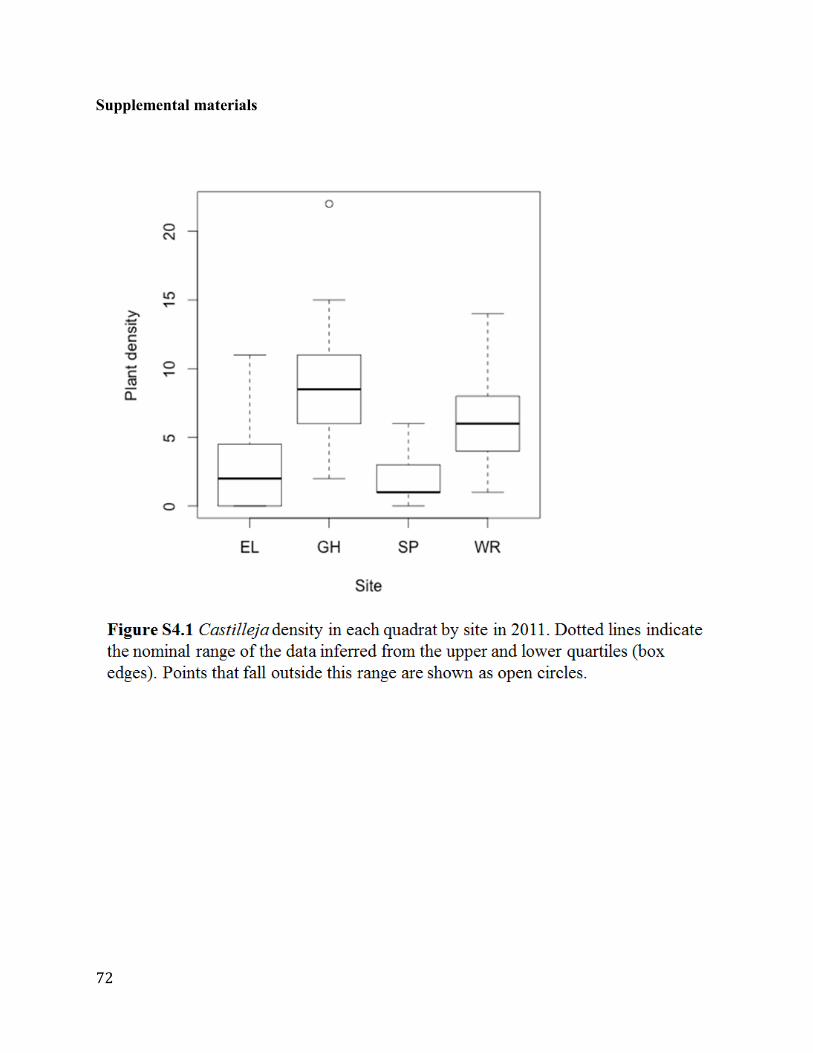
72

Supplemental materials

73

74

75

Chapter 5: Synthesis

Over the course of research for the previous chapters, we found clear differences in parasite

survival, growth, and reproduction related to host identity (Chapter 2). Host species’

contributions to these traits in Castilleja levisecta fluctuated over the two years of monitoring,

and we found that total seed capsule numbers were highest in C. levisecta planted with Achillea

millefolium and Danthonia californica (Figure 2.6). This metric is among the most important in

restoration and conservation goals, as it creates greater opportunity for new or recovering

populations to become sustainable. These results contribute valuable novel hosts to the tools

used in management of this threatened species.

Clear differences were also present in the nutrition derived from different host species by C.

levisecta (Chapter 3). Nitrogen was more variable than carbon, and the highest contributor to

parasite tissue nitrogen was Eriophyllum lanatum (Figure 3.3). This may indicate one

mechanism by which a host can benefit Castilleja, but when compared to results from chapter 1,

it may be one of several indicators of host quality.

When results from chapters two and three are combined (using the species or genera that

overlapped between the two experiments), the top hosts for overall Castilleja performance are

Achillea millefolium, Danthonia californica, and Eriophyllum lanatum (Table 5.1). LULE and

LULI were combined using LULI data from Chapter 2 (no LULI pairs survived and thus were

not included in that analysis), and the LULE data from Chapter 3. It should be noted that of

these three, only Eriophyllum is used as a common host in the literature. The other two are

rarely, if ever, cited in the literature as hosts of this Castilleja species. These new suggestions

76

for host species can inform land management practices in the reintroduction and conservation of

this threatened species.

Table 5.1 Comparative rankings of Castilleja performance with each host species in chapters 2

and 3. Ratings are based on each variable in positive relation to performance (best performance

= 1, worst performance = 7). Ranks 1-2 are bolded and ranks 6-7 are grayed. See Tables 2.1 and

3.1 for full species names.

ACMI DACA ERLA ERSP FERO

LULI/

LULE

SOCA/

SOMI

Survival 2013 1 2 5 7 5 3 5

Flowering stems 13 1 4 5.5 2 5.5 3 7

Browsed stems 13 1 3 4 2 5 6.5 6.5

Plants browsed 6.5 5 3.5 6.5 3.5 1.5 1.5

Height 2013 1 2 6 3 5 4 7

Fruiting stems 13 1 2 4 5 3 7 6

Seed capsules 13 1 2 4 7 3 5 6

Survival 14 4.5 1 2 6.5 3 4.5 6.5

Flowering stems 14 4 5 1 3 2 6 7

Browsed stems 14 1 3 2 7 4 6 5

Plants browsed 7 5 6 2 4 2 2

Height 14 4 6 2 5 3 1 7

Fruiting stems 14 1 4 2 5.5 3 5.5 7

Seed capsules 14 3 1 2 5 4 6 7

Carbon (isotope) 5 3 2 7 4 6 1

Nitrogen (isotope) 2 5 1 7 3 6 4

Average Rank 2.8 3.3 3.3 5.0 3.8 4.6 5.3

While we found ample evidence for surrounding plants’ effects on Castilleja, there was less

evidence for the reverse effect of the parasite on the community (Chapter 4). Studies in other

systems have shown significant effects of parasites on community composition and richness, but

some had limited spatial and temporal scale of monitoring (e.g. Bao et al. 2015). Our analysis

did find significant effects of parasites in some cases, but no clear pattern at a larger scale of

space and time (Chapter 4).

77

Together, these studies demonstrate the complexity of parasite-community relationships and

point to areas of research for future studies. Given the generalist nature of many hemiparasites,

it is likely that investigation of a variety of hosts could yield valuable insights into parasitic

relationships. More research should be done to uncover the mechanisms behind host quality,

including not just carbon and nitrogen, but additional macronutrients, water, and defensive

compounds. This would give a more holistic view of host contributions to this parasite. Finally,

there is a need for more long-term studies than span a greater geographical area to elucidate a

generalized theory of parasite community effects. Collaborative studies such as the Nutrient

Network (including Grace et al. 2016) point to a method of achieving this goal.

78

All References

Adler, L.S. 2002. Host Effects on Herbivory and Pollination in a Hemiparasitic Plant. Ecology,

83(10): 2700-2710.

Adler, L.S. 2003. Host species affects herbivory, pollination, and reproduction in experiments

with parasitic Castilleja. Ecology, 84(8):2083–2091.

Adler, L.S. and M. Wink. 2001. Transfer of alkaloids from hosts to hemiparasites in two

Castilleja-Lupinus associations: analysis of floral and vegetative tissues. Biochemical

Systematics and Ecology, 29: 551-561.

Aflakpui, G.K.S., P.J. Gregory, and R.J. Froud-Williams. 2005. Carbon (13C) and Nitrogen

(15N) translocation in a Maize-Striga hermonthica association. Experimental Agriculture, 41(3):

321-333.

Altman, B. 2011. Historical and Current Distribution and Populations of Bird Species in Prairie-

Oak Habitats in the Pacific Northwest. Northwest Science, 85:194–222.

Bao, G.S., K. Suetsugu, H.S. Wang, X. Yao, L. Liu, J. Ou, and C.J. Li. 2015. Effects of the

hemiparasitic plant Pedicularis kansuensis on plant community structure in a degraded

grassland. Ecological Research, 30(3): 507-515.

Boyd, R. 1999. Indians, Fire, and the Land in the Pacific Northwest. Page 320. Oregon State

University Press, Corvallis, OR.

Bullock, J.M and R.F. Pywell. 2005. Rhinanthus: A tool for restoring diverse grasslands?. Folia

Geobotanica, 40(2-3): 273-288.

Butchart, S.H.M. et al. 2010. Global Biodiversity: Indicators of Recent Declines. Science,

328(5982): 1164-1168.

Cameron, D.D., A. White, and J. Antonovics. 2009. Parasite–grass–forb interactions and rock–

paper– scissor dynamics: predicting the effects of the parasitic plant Rhinanthus minor on host

plant communities. Journal of Ecology, 97(6): 1311-1319.

Cameron, D.D., A.M. Coats, and W.E. Seel. 2006. Differential Resistance among Host and Non-

host Species Underlies the Variable Success of the Hemi-parasitic Plant Rhinanthus minor.

Annals of Botany, 98(6): 1289-1299.

Caplow, F. 2004. Reintroduction plan for golden paintbrush (Castilleja levisecta). Prepared for

U.S. Fish and Wildlife Service. Page 87. Olympia, WA.

Crawford, R. C., and H. Hall. 1997. Changes in the South Puget Sound Prairie Landscape. Pgs

11–16. Ecology and Conservation of the South Puget Sound Prairie Landscape. P.W.

Dunnwiddie and K. Ewing eds. The Nature Conservancy. Seattle, WA.

79

Davies, D.M., J.D. Graves, C.O. Elias, and P.J. Williams. 1997. The impact of Rhinanthus spp.

on sward productivity and composition: Implications for the restoration of species-rich

grasslands. Biological Conservation, 82(1): 87-93.

Decleer, K., D. Bonte, and R. Van Diggelen. 2013. The hemiparasite Pedicularis palustris:

‘Ecosystem engineer’ for fen-meadow restoration. Journal for Nature Conservation, 21(2): 65-

71.

Delvin, E. 2013. Restoring Abandoned Agricultural Lands in Puget Lowland Prairies: A New

Approach. PhD Thesis, University of Washington. Seattle, WA.

Demey, A., P. De Frenne, L. Baeten, G. Verstraeten, M. Hermy, P. Boeckx, and K. Verheyen.

2015. The effects of hemiparasitic plant removal on community structure and seedling

establishment in semi-natural grasslands. Journal of Vegetation Science, 26(3): 409-420.

Demey, A., T. Rutting, D. Huygens, J. Staelens, M. Hermy, K. Verheyen, and P. Boeckx. 2014.

Hemiparasitic litter additions alter gross nitrogen turnover in temperate semi-natural grassland

soils. Soil Biology and Biochemistry, 68: 419-428.

Dobbins, D.R. and J. Kuijt. 1973. Studies on the haustorium of Castilleja (Scrophulariaceae). I.

The upper haustorium. Canadian Journal of Botany, 51: 917–922.

Ducharme, L.A. and J.R. Ehlringer. 1996. Gas exchange, delta C-13, and hetertrophy for

Castilleja linariifolia and Orthocarpus tolmiei, facultative root hemiparasites on Artemisia

tridentata. Great Basin Naturalist, 56(4): 333-340.

Dunwiddie, P.W. 2002. Management and restoration of grasslands on Yellow Island, San Juan

Islands, Washington, USA. Pgs 78-87. Garry Oak Ecosystem Restoration: Progress and

Prognosis. Proceedings of the Third Annual Meeting of the B.C. Chapter of the Society for

Ecological Restoration, April 27-28, 2002, P. J. Burton ed. University of Victoria. B.C. Chapter

of the Society for Ecological Restoration, Victoria, British Columbia.

Dunwiddie, P., and J.D. Bakker. 2011. The Future of Restoration and Management of Prairie-

Oak Ecosystems in the Pacific Northwest. Northwest Science 85: 83–92.

Dunwiddie, P. and J.D. Bakker. 2011. Personal Communication.

Dunwiddie, P. and R.A. Martin. 2016. Microsites matter: Improving the success of rare species

reintroductions. PLoS One 11(3): e0150417.

Dunwiddie, P.W., N.L. Haan, M. Linders, J.D. Bakker, C. Fimbel, and T.B. Thomas. 2016.

Intertwined fates: Opportunities and challenges in the linked recovery of two rare species.

Natural Areas Journal, 36(2): Accepted for publication.

80

Evans, R.D., and J.R. Ehleringer. Plant δ15N values along a fog gradient in the Atacama Desert,

Chile. Journal of Arid Environments, 28(3): 189-193.

Fazzino, L., H.E. Kirkpatrick, and C. Fimbel. 2011. Comparison of Hand-Pollinated and

Naturally-Pollinated Puget Balsamroot (Balsamorhiza deltoidea Nutt.) to Determine Pollinator

Limitations on South Puget Sound Lowland Prairies. Northwest Science, 85: 352–360.

Fisher, J.P., G.K. Phoenix, D.Z. Childs, M.C. Press, S.W. Smith, M.G. Pilkington, and D.D.

Cameron. 2013. Parasitic plant litter input: a novel indirect mechanism influencing plant

community structure. New Phytologist, 198(1): 222-231.

Fisher, L., J.D. Bakker, and P.W. Dunwiddie. 2015. An Assessment of Seed Production and

Viability of Putative Castilleja levisecta × C. hispida Hybrids. Report for the Center for Natural

Lands Management.

Franklin, J. F., and C. T. Dyrness. 1988. Natural vegetation of Oregon and Washington. Oregon

State University Press.

Grace, J.B. et al. 2016. Integrative modelling reveals mechanisms linking productivity and plant

species richness. Nature, 529: 390-393.

Grewell, B.J. 2008. Hemiparasites generate environmental heterogeneity and enhance species

coexistence in salt marshes. Ecological Applications, 18(5): 1297-1306.

Gurney, A.L., D. Grimanelli, F. Kanampiu, D. Hoisington, J.D. Scholes, and M.C. Press. 2003.

Novel sources of resistance to Striga hermonthica in Tripsacum dactyloides, a wild relative of

maize. New Phytologist, 160(3): 557-568.

Haan, N. 2015. Unpublished data.

Hartley, S.E., J.P. Green, F.P. Massey, M.C.P. Press, A.J.A. Stewart, and E.A. John. 2015.

Hemiparasitic plant impacts animal and plant communities across four trophic levels. Ecology,

96(9): 2408-2416.

Hautier, Y., A. Hector, E. Vojtech, D. Purves, and L.A. Turnbull. 2010. Modelling the growth of

parasitic plants. Journal of Ecology, 98(4): 857–866.

Heckard, L.R. 1962. Root parasitism in Castilleja. Botanical Gazette, 124(1): 21-29. Kaye, T.N.,

K. Jones, and I. Pfingsten. 2011. Reintroduction of golden paintbrush to Oregon: 2011 Annual

Report to the U.S. Fish and Wildlife Service. Institute for Applied Ecology, Corvallis, OR.

Kohn, M.J. 2010. Carbon isotope compositions of terrestrial C3 plants as indicators of

(paleo)ecology and (paleo)climate. Proceedings of the National Academy of Sciences of the

United States of America, 107(46): 19691-19695.

81

Kuijt, J. 1969. The biology of parasitic flowering plants. University of California Press,

Berkeley, CA.

Lawrence, B.A. and T.N. Kaye. 2011. Reintroduction of Castilleja levisecta: Effects of

ecological similarity, source population genetics, and habitat quality. Restoration Ecology,

19(2):166-176.

Lawrence, B.A. and T.N. Kaye. 2008. Direct and indirect effects of host plants: implications for

reintroduction of an endangered hemiparasitic plant (Castilleja levisecta). Madroño, 55(2):151–

158.

Lawrence, B.A. 2005. Studies to Facilitate Reintroduction of Golden Paintbrush (Castilleja

levisecta) to the Willamette Valley, Oregon. MS thesis. Oregon State University.

Leroy, C., N. Sejalon-Delmas, A. Jauneau, M.X. Ruiz-Gonzales, H. Gryta, P. Jargeat, B.

Corbara, A. Dejean, and J. Orivel. 2011. Trophic mediation by a fungus in an ant-plant

mutualism. Journal of Ecology, 99(2): 583-590.

Li, A.R., Y.J. Li, S.E. Smith, F.A. Smith, and K.Y. Guan. 2013. Nutrient requirements differ in

two Pedicularis species in the absence of a host plant: implication for driving forces in the

evolution of host preference of root hemiparasitic plants. Annals of Botany, 112(6): 1099-1106.

Marko, M.D. and F.R. Stermitz. 1997. Transfer of alkaloids from Delphinium to Castilleja via

root parasitism. Norditerpenoid alkaloid analysis by electrospray mass spectrometry.

Biochemical Systematics and Ecology, 25(4): 279-285.

Marko, M.D. and F.R. Stermitz. 1997. Transfer of alkaloids from Delphinium to Castilleja via

root parasitism. Norditerpenoid alkaloid analysis by electrospray mass spectrometry.

Biochemical Systematics and Ecology, 25(4): 279-285.

Marshall, J.D., J.R. Ehleringer, E.D. Schulze, and G.D. Farquhar. 1994. Carbon isotope

composition, gas exchange and heterotrophy in Australian mistletoes. Functional Ecology, 8:

237-241.

Marshall, J.D. and J.R. Ehleringer. 1990. Are xylem tapping mistletoes partially heterotrophic?

Oecologia, 84: 244-248.

Marvier, M. 1998. A mixed diet improves performance and herbivore resistance of a parasitic

plant. Ecology, 79(4): 1272-1280.

McKinney, M.L. and J.L. Lockwood. 1999. Biotic homogenization: a few winners replacing

many losers in the next mass extinction. Trends in Ecology and Evolution 14: 450–453.

Mumera, L.M. and F.E. Below. 1993. Role of nitrogen in resistance to Striga parasitism of

maize. Crop Science, 33(4): 758-763.

82

Nickrent, D.L., R.J. Duff, A.E. Colwell et al. 1998. Molecular phylogenetic and evolutionary

studies of parasitic plants. In: Soltis, DE, P.S. Soltis, J.J. Doyle, eds. Molecular Systematics of

Plants II DNA Sequencing. Boston, USA: Kluwer Academic, 211-241.

Oksanen, J., F. G. Blanchet, R. Kindt, P. Legendre, P.R. Minchin, R.B. O'Hara, G.L. Simpson, P.

Solymos, M. Henry, H. Stevens, and H. Wagner. 2015. vegan: Community Ecology Package. R

package version 2.3-1. https://CRAN.R-project.org/package=vegan

Pageau, K., P. Simier, N. Naulet, R. Robins, and A. Fer. 1998. Carbon dependency of the

hemiparasite Striga hermonthica on Sorghum bicolor determined by carbon isotopic and gas

exchange analyses. Australian Journal of Plant Physiology, 25: 695-700.

Pate, J.S., K.C. True, and E. Rasins. 1991. Xylem transport and storage of amino acids by S. W.

Australian mistletoes and their hosts. Journal of Experimental Botany, 42: 441-451.

Philip, L.J. and S.W. Simard. 2008. Minimum pulses of stable and radioactive carbon isotopes to

detect belowground carbon transfer between plants. Plant Soil, 308 (1-2): 23-25.

Phoenix, G.K. and M.C. Press. 2005. Linking physiological traits to impacts on community

structure and function: the role of root hemiparasitic Orobanchaceae (ex-Scrophulariaceae).

Journal of Ecology, 93(1): 67-78.

Press, M.C. 1998. Dracula or Robin Hood? A functional role for root hemiparasites in nutrient

poor ecosystems. Oikos, 82(3): 609-611.

Press, M.C. and G.K. Phoenix. 2005. Impacts of parasitic plants on natural communities. New

Phytologist, 166(3): 737-751.

Pywell, R.F., J.M. Bullock, K.J. Walker, S.J. Coulson, S.J. Gregory, and M.J. Stevenson. 2004.

Facilitating grassland diversification using the hemiparasitic plant Rhinanthus minor. Journal of

Applied Ecology, 41(5): 880-887.

Quested, H.M., T.V. Callaghan, J.H.C. Cornelissen, and M.C. Press. 2005. The impact of

hemiparasitic plant litter on decomposition: direct, seasonal and litter mixing effects. Journal of

Ecology, 93(1): 87-98.

Rowntree, J.K., D.F. Barham, A.J.A. Stewart, and S.E. Hartley. 2014. The effect of multiple host

species on a keystone parasitic plant and its aphid herbivores. Functional Ecology, 28(4): 829–

836.

Rümer, S., D.D. Cameron, R. Wacker, W. Hartung, & F. Jiang. 2007. An anatomical study of the

haustoria of Rhinanthus minor attached to roots of different hosts. Flora 202(3): 194–202.

Schmidt, D. 1998.Restoraion of a Prairie Ecosystem at the Yellow Island Preserve and the

Propagation of Castilleja hispida by Vegetative Cuttings. Master’s Thesis, University of

Washington. Seattle, WA.

83

Schulze, E.D., O.L. Lange, H. Zeigler, and G. Gebaur. 1991. Carbon and nitrogen isotope ratios

of mistletoes growing on nitrogen and non nitrogen fixing hosts and on CAM plants in the

Namib desert confirm partial heterotrophy. Oecologia, 88: 457-462.

Schultz, C.B., E. Henry, A. Carleton, T. Hicks, R. Thomas, A. Potter, M. Linders, C.

Fimbel, S. Black, H.E. Anderson, G. Diehl, S. Hamman, J. Foster, D. Hays, D.

Wilderman, R. Davenport, E. Steel, N. Page, P.L. Lilley, J. Heron, N. Kroeker, C.

Webb, and B. Reader. 2011. Conservation of Prairie-Oak Butterflies in Oregon,

Washington, and British Columbia. Northwest Science, 85: 361–388.

Severns, P.M., and A.D. Warren. 2008. Selectively eliminating and conserving exotic plants to

save an endangered butterfly from local extinction. Animal Conservation, 11(6): 476-483.

Smith, F.D., R.M. May, R. Pellew, T.H. Johnson, and K.S. Walter. 1993. Estimating extinction

rates. Nature, 364: 494–496.

Spallek, T., M. Mutuku, and K. Shirasu. 2013. The genus Striga: a witch profile. Molecular Plant

Pathology, 14(9): 861-869.

Stanton, S. 2006. The differential effects of dwarf mistletoe infection and broom abundance on

the radial growth of managed ponderosa pine. Forest Ecology and Management, 223(1-3): 318-

326.

Stermitz, F.R. and G.H. Harris. 1987. Transfer of pyrrolizidine and quinolizidine alkaloids to

Castilleja (Scrophulariaceae) hemiparasites from composite and legume host plants. Journal of

Chemical Ecology, 13(8): 1917-1925.

Stermitz, F.R. and M. Pomeroy. 1992. Iridoid glycosides from Castilleja purpurea and C.

indivisa, and quinolizidine alkaloid transfer from Lupinus texensis to C. indivisa via root

parasitism. Biochemical Systematics and Ecology, 20: 473-475.

Stinson, D. 2005. Washington State Status Report for the Mazama Pocket Gopher,

Streaked Horned Lark, and Taylor’s Checkerspot. Page 129 + xii pp. Washington

Department of Fish and Wildlife. Olympia.

Tesitel, J., T. Tesitelova, J.P. Fisher, J. Leps, and D.D. Cameron. 2015. Integrating ecology and

physiology of root-hemiparasitic interaction: interactive effects of abiotic resources shape the

interplay between parasitism and autotrophy. New Phytologist, 205(1): 350-360.

Tesitel, J., J. Leps, M. Vrablova, and D.D. Cameron. 2011. The role of heterotrophic carbon

acquisition by the hemiparasitic plant Rhinanthus alectorophus in seedling establishment in

natural communities: a physiological perspective. New Phytologist, 192(1): 188-199.

84

Tesitel, J., L. Plavcova, and D.D. Cameron. 2010. Heterotrophic carbon gain by the root

hemiparasites, Rhinanthus minor and Euphrasia rostkoviana (Orobanchaceae). Planta, 231(5):

1137-114.

USFWS (U.S. Fish and Wildlife Service). 2000. Recovery Plan for Golden Paintbrush (Castilleja

levisecta). U.S. Fish and Wildlife Service, Portland, Oregon.

Vitousek, P.M. 1992. Global Environmental Change - An Introduction. Annual Review of

Ecology and Systematics, 23: 1-14.

Watson, D.M. 2009. Parasitic plants as facilitators: more Dryad than Dracula? Journal of

Ecology, 97: 1151-1159.

Wentworth, J. B. 2001. The demography and population dynamics of Castilleja levisecta, a

federally threatened perennial of Puget Sound Grasslands. Pages 49–51 in R. S. Reichard, P.

Dunwiddie, J. Gamon, A. Kruckeberg, and D. Salstrom, editors. Conservation of Washington’s

Native Plants and Ecosystems. Washington Native Plant Society, Seattle.

Westbury, D.B., A. Davies, B.A. Woodcock, and N.P. Dunnett. 2006. Seeds of change: The

value of using Rhinanthus minor in grassland restoration. Journal of Vegetation Science, 17(4):

435-446.

85

Appendix A: ‘R’ code used for Chapter 2 analyses

### Load packages

library(plyr)

library(lsmeans)

library(ggplot2)

field.data<-read.csv(file.choose(), header=TRUE)

# choose 'Cleaned_Field_Companion_Data151126.csv'; 260 x 33

### Take out '2 CALE' triplets (omit; not mortality)

fd.all <- field.data[field.data$Notes_Spr13 == "0", ] # 256 x 33

fd.all.summary <- ddply(fd.all, .(Host.ID), summarize, N = length(ID.Number))

### Analyze 2013 and 2014 survival (focusing only on those plantings where both the

CALE and host survived)

fd.all$Live_Spr13 <- ifelse(fd.all$CALE.alive_Spr13 == 1 & fd.all$Host.alive_Spr13 == 1, 1, 0)

sum(fd.all$Live_Spr13) # 109 observations

fd.all$Live_Spr14 <- ifelse(fd.all$CALE.alive_Spr14 == 1 & fd.all$Host.alive_Spr14 == 1, 1, 0)

sum(fd.all$Live_Spr14) # 67 observations

Surv.13 <- glm(Live_Spr13 ~ Host.ID, data = fd.all, family = binomial)

summary(Surv.13)

anova(Surv.13, update(Surv.13, ~ . - Host.ID), test="Chisq") # host effect significant

lsmeans(Surv.13, "Host.ID", contr = "trt.vs.ctrl", adjust = "none") # ACMI, DECA, (DACA)

lsmeans(Surv.13, specs = pairwise ~ Host.ID, adjust = "none")

Surv.14 <- glm(Live_Spr14 ~ Host.ID, data = fd.all, family = binomial)

summary(Surv.14)

anova(Surv.14, update(Surv.14, ~ . - Host.ID), test="Chisq") # host effect significant

lsmeans(Surv.14, "Host.ID", contr = "trt.vs.ctrl", adjust = "none") # DECA, (DACA)

lsmeans(Surv.14, specs = pairwise ~ Host.ID, adjust = "none")

fd.survival <- ddply(fd.all, .(Host.ID), summarize,

N = length(Live_Spr13),

N.live13 = sum(Live_Spr13),

prop.live13 = N.live13 / N,

N.live14 = sum(Live_Spr14),

prop.live14 = N.live14 / N)

### Focus on live plants in 2013 (those where both CALE and host are alive)

fd.live13 <- fd.all[fd.all$Live_Spr13 == 1, ] # 109 x 35

fd.live13$Flowering.stems_Spr13<-as.numeric(fd.live13$Flowering.stems_Spr13)

fd.live13$Browsed.stems_Spr13<-as.numeric(fd.live13$Browsed.stems_Spr13)

fd.live13$CALE.height_Spr13<-as.numeric(fd.live13$CALE.height_Spr13)

86

fd.live13$Fruiting.Stems_Fall13<-as.numeric(fd.live13$Fruiting.Stems_Fall13)

fd.live13$Total.pods_Fall13<-as.numeric(fd.live13$Total.pods_Fall13)

fd.live13$Browsed.Plants_Spr13 <- ifelse(fd.live13$Browsed.stems_Spr13 > 0, 1, 0)

fd.live13.summary <- ddply(fd.live13, .(Host.ID), summarize,

Flowering.stems = mean(Flowering.stems_Spr13),

Flowering.stems = mean(Flowering.stems_Fall13),

Browsed.stems = mean(Browsed.stems_Spr13),

Browsed.Plants = sum(Browsed.Plants_Spr13),

CALE.height = mean(CALE.height_Spr13),

Fruiting.Stems = mean(Fruiting.Stems_Fall13),

Total.pods = mean(Total.pods_Fall13),

N.live = sum(Live_Spr13))

fd.live13.summary <- merge(fd.live13.summary, fd.all.summary, by = "Host.ID", all.y =

FALSE)

### glm

Spr.flow.stem.13 <- glm(Flowering.stems_Spr13 ~ Host.ID, data=fd.live13, family=poisson)

summary(Spr.flow.stem.13)

anova(Spr.flow.stem.13, update(Spr.flow.stem.13, ~ . - Host.ID), test = "Chisq") #significant

lsmeans(Spr.flow.stem.13, "Host.ID", contr = "trt.vs.ctrl", adjust = "none") # ACMI, DECA,

(SYAL) lsmeans(Spr.flow.stem.13, specs = pairwise ~ Host.ID, adjust = "none")

Spr.brow.stem.13<-glm(Browsed.stems_Spr13 ~ Host.ID, data=fd.live13, family=poisson)

summary(Spr.brow.stem.13)

anova(Spr.brow.stem.13, update(Spr.brow.stem.13, ~ . - Host.ID), test = "Chisq") #significant

lsmeans(Spr.brow.stem.13, "Host.ID", contr = "trt.vs.ctrl", adjust = "none") # DECA, FERO,

SYAL, (ACMI) lsmeans(Spr.brow.stem.13, specs = pairwise ~ Host.ID, adjust = "none")

Browsed.plants.13<-glm(Browsed.Plants_Spr13 ~ Host.ID, data=fd.live13, family=binomial)

summary(Browsed.plants.13)

anova(Browsed.plants.13, update(Browsed.plants.13, ~ . - Host.ID), test = "Chisq") #significant

lsmeans(Browsed.plants.13, "Host.ID", contr = "trt.vs.ctrl", adjust = "none") # NS

lsmeans(Browsed.plants.13, specs = pairwise ~ Host.ID, adjust = "none")

CALEheight.13 <- lm(CALE.height_Spr13 ~ Host.ID, data=fd.live13)

summary(CALEheight.13)

anova(CALEheight.13, update(CALEheight.13, ~ . - Host.ID)) #significant

lsmeans(CALEheight.13, "Host.ID", contr = "trt.vs.ctrl", adjust = "none") # ACMI, DECA

lsmeans(CALEheight.13, specs = pairwise ~ Host.ID, adjust = "none")

fruit.stem.13 <- glm(Fruiting.Stems_Fall13 ~ Host.ID, data=fd.live13, family=poisson)

summary(fruit.stem.13)

#need to drop control because none had fruiting stems

87

fruit.stem.13 <- glm(Fruiting.Stems_Fall13 ~ Host.ID, data=fd.live13[fd.live13$Host.ID != "aa

No Host",], family=poisson)

summary(fruit.stem.13)

anova(fruit.stem.13, update(fruit.stem.13, ~ . - Host.ID), test = "Chisq") #significant

lsmeans(fruit.stem.13, specs = pairwise ~ Host.ID, adjust = "none")

seedpods.13 <- glm(Total.pods_Fall13 ~ Host.ID, data = fd.live13, family = poisson)

summary(seedpods.13)

#need to drop control because none had fruiting stems

seedpods.13 <- glm(Total.pods_Fall13 ~ Host.ID, data=fd.live13[fd.live13$Host.ID != "aa No

Host",], family=poisson)

summary(seedpods.13)

anova(seedpods.13, update(seedpods.13, ~ . - Host.ID), test = "Chisq") #significant

lsmeans(seedpods.13, specs = pairwise ~ Host.ID, adjust = "none")

### Focus on live plants in 2014 (those where both CALE and host are alive)

fd.live14 <- fd.all[fd.all$Live_Spr14 == 1, ] # 67 x 35

fd.live14$Flowering.stems_Spr14<-as.numeric(fd.live14$Flowering.stems_Spr14)

fd.live14$Browsed.stems_Spr14<-as.numeric(fd.live14$Browsed.stems_Spr14)

fd.live14$CALE.height_Spr14<-as.numeric(fd.live14$CALE.height_Spr14)

fd.live14$Fruiting.Stems_Fall14<-as.numeric(fd.live14$Fruiting.Stems_Fall14)

fd.live14$Total.pods_Fall14<-as.numeric(fd.live14$Total.pods_Fall14)

fd.live14$Browsed.Plants_Spr14 <- ifelse(fd.live14$Browsed.stems_Spr14 > 0, 1, 0)

fd.live14.summary <- ddply(fd.live14, .(Host.ID), summarize,

Flowering.stems = mean(Flowering.stems_Spr14),

Flowering.stems = mean(Flowering.stems_Fall14),

Browsed.stems = mean(Browsed.stems_Spr14),

Browsed.Plants = sum(Browsed.Plants_Spr14),

CALE.height = mean(CALE.height_Spr14),

Fruiting.Stems = mean(Fruiting.Stems_Fall14),

Total.pods = mean(Total.pods_Fall14),

N.live = sum(Live_Spr14))

fd.live14.summary <- merge(fd.live14.summary, fd.all.summary, by = "Host.ID", all.y =

FALSE)

### glm

Spr.flow.stem.14 <- glm(Flowering.stems_Spr14 ~ Host.ID, data=fd.live14, family=poisson)

summary(Spr.flow.stem.14)

anova(Spr.flow.stem.14, update(Spr.flow.stem.14, ~ . - Host.ID), test = "Chisq") #significant

lsmeans(Spr.flow.stem.14, "Host.ID", contr = "trt.vs.ctrl", adjust = "none") # ERLA, DECA,

FERO, SYAL, ERSP, DACA, ACMI, LULI lsmeans(Spr.flow.stem.14, specs = pairwise ~ Host.ID, adjust = "none")

Spr.brow.stem.14<-glm(Browsed.stems_Spr14 ~ Host.ID, data=fd.live14, family=poisson)

88

summary(Spr.brow.stem.14)

anova(Spr.brow.stem.14, update(Spr.brow.stem.14, ~ . - Host.ID), test = "Chisq") #significant

lsmeans(Spr.brow.stem.14, "Host.ID", contr = "trt.vs.ctrl", adjust = "none") # ACMI, LULI,

ERSP, RONU, SYAL, (DECA) lsmeans(Spr.brow.stem.14, specs = pairwise ~ Host.ID, adjust = "none")

Browsed.plants.14<-glm(Browsed.Plants_Spr14 ~ Host.ID, data=fd.live14, family=binomial)

summary(Browsed.plants.14)

anova(Browsed.plants.14, update(Browsed.plants.14, ~ . - Host.ID), test = "Chisq") #NS

lsmeans(Browsed.plants.14, specs = pairwise ~ Host.ID, adjust = "none")

CALEheight.14 <- lm(CALE.height_Spr14~ Host.ID, data=fd.live14)

summary(CALEheight.14)

anova(CALEheight.14, update(CALEheight.14, ~ . - Host.ID)) #significant

lsmeans(CALEheight.14, "Host.ID", contr = "trt.vs.ctrl", adjust = "none") # LULI, ERLA,

FERO, DECA, ACMI, (DACA), (SYAL) lsmeans(CALEheight.14, specs = pairwise ~ Host.ID, adjust = "none")

fruit.stem.14 <- glm(Fruiting.Stems_Fall14 ~ Host.ID, data=fd.live14, family=poisson)

summary(fruit.stem.14)

anova(fruit.stem.14, update(fruit.stem.14, ~ . - Host.ID), test = "Chisq") #significant

lsmeans(fruit.stem.14, "Host.ID", contr = "trt.vs.ctrl", adjust = "none") # ACMI, ERLA, FERO,

DACA, SYAL, DECA, (LULI) lsmeans(fruit.stem.14, specs = pairwise ~ Host.ID, adjust = "none")

seedpods.14 <- glm(Total.pods_Fall14 ~ Host.ID, data = fd.live14, family = poisson)

summary(seedpods.14)

anova(seedpods.14, update(seedpods.14, ~ . - Host.ID), test = "Chisq") #significant

lsmeans(seedpods.14, "Host.ID", contr = "trt.vs.ctrl", adjust = "none") # ERLA, DACA, ACMI,

FERO, SYAL, DECA, ERSP, RONU, LULI lsmeans(seedpods.14, specs = pairwise ~ Host.ID, adjust = "none")

#### Combine survival and seed production in both years

fd.live13.summary$s13xcap13 <- fd.live13.summary$Total.pods * (fd.live13.summary$N.live /

fd.live13.summary$N) * 100

fd.live14.summary$s14xcap14 <- fd.live14.summary$Total.pods * (fd.live14.summary$N.live /

fd.live14.summary$N) * 100

fd.summary <- merge(x = fd.live13.summary[, c("Host.ID", "s13xcap13")],

y = fd.live14.summary[, c("Host.ID", "s14xcap14")])

fd.summary$Total <- fd.summary$s13xcap13 + fd.summary$s14xcap14

write.table(fd.summary, "/users/christopherjones/fd.summary.txt", sep="\t")

89

fd.live13.summary$Perc.browsed<-(fd.live13.summary$Browsed.Plants /

fd.live13.summary$N.live) * 100

fd.live14.summary$Perc.browsed<-(fd.live14.summary$Browsed.Plants /

fd.live14.summary$N.live) * 100

### graphs

par(mfrow=c(1,2))

### flowering stems

plot(Flowering.stems_Spr13 ~ Host.ID, data=fd.live13, las=3, xlab="", ylab="Flowering Stems

Spring 2013", ylim = c(0, 15))

plot(Flowering.stems_Spr14 ~ Host.ID, data=fd.live14, las=3, xlab="", ylab="Flowering Stems

Spring 2014", ylim = c(0, 15))

### browsed stems

plot(Browsed.stems_Spr13 ~ Host.ID, data=fd.live13, las=3, xlab="", ylab="Browsed Stems

Spring 2013", ylim = c(0, 25))

plot(Browsed.stems_Spr14 ~ Host.ID, data=fd.live14, las=3, xlab="", ylab="Browsed Stems

Spring 2014", ylim = c(0, 25))

### height

plot(CALE.height_Spr13 ~ Host.ID, data=fd.live13, las=3, xlab="", ylab="Height Spring 2013",

ylim = c(0, 70))

plot(CALE.height_Spr14 ~ Host.ID, data=fd.live14, las=3, xlab="", ylab="Height Spring 2014",

ylim = c(0, 70))

### fruiting stems

plot(Fruiting.Stems_Fall13 ~ Host.ID, data=fd.live13, las=3, xlab="", ylab="Fruiting Stems Fall

2013", ylim = c(0, 16))

plot(Fruiting.Stems_Fall14 ~ Host.ID, data=fd.live14, las=3, xlab="", ylab="Fruiting Stems Fall

2014", ylim = c(0, 16))

### seed capsule number

plot(Total.pods_Fall13 ~ Host.ID, data=fd.live13, las=3, xlab="", ylab="Seed capsules Fall

2013", ylim = c(0, 160))

plot(Total.pods_Fall14 ~ Host.ID, data=fd.live14, las=3, xlab="", ylab="Seed capsules Fall

2014", ylim = c(0, 160))

90

### percent of live plants browsed

plot(fd.live13.summary$Host.ID, fd.live13.summary$Perc.browsed, las=3, xlab="", ylab="%

live plants browsed Spring 2013", ylim = c(0, 100))

plot(fd.live14.summary$Host.ID, fd.live14.summary$Perc.browsed, las=3, xlab="", ylab="%

live plants browsed Spring 2014", ylim = c(0, 100))

91

Appendix B: ‘R’ code used for Chapter 3 analyses

iso <- read.csv(file.choose(), header = TRUE) #Use ‘Iso_Data_Final’

iso$Host<-as.factor(iso$Host)

iso$del.C<-as.numeric(iso$del.C)

iso$del.N<-as.numeric(iso$del.N)

library(PMCMR)

diff.N <- kruskal.test(del.N ~ Host, data=iso)

diff.N

posthoc.kruskal.nemenyi.test(del.N ~ Host, data = iso)

diff.C <- kruskal.test(del.C ~ Host, data=iso)

diff.C

posthoc.kruskal.nemenyi.test(del.C ~ Host, data = iso)

library(lsmeans)

diff.N <- aov(del.N ~ Host, data=iso)

summary(diff.N)

lsmeans(diff.N, specs = pairwise ~ Host, adjust = "none")

diff.C <- aov(del.C ~ Host, data=iso)

summary(diff.C)

lsmeans(diff.C, specs = pairwise ~ Host, adjust = "none")

### plot all C vs N

plot(iso$del.C, iso$del.N, main = "All groups", xlab = "del 13C", ylab = "del 15N")

### plot each host group C vs N

iso.ACMI<-iso[iso$Host == "ACMI",]

iso.DACA<-iso[iso$Host == "DACA",]

iso.ERLA<-iso[iso$Host == "ERLA",]

iso.ERSP<-iso[iso$Host == "ERSP",]

iso.FERO<-iso[iso$Host == "FERO",]

iso.LULE<-iso[iso$Host == "LULE",]

iso.SOMI<-iso[iso$Host == "SOMI",]

par(mfrow=c(1,1))

plot(iso.ACMI$del.C, iso.ACMI$del.N, main = "ACMI group", xlab = "del 13C", ylab = "del

15N")

plot(iso.DACA$del.C, iso.DACA$del.N, main = "DACA group", xlab = "del 13C", ylab = "del

15N")

plot(iso.ERLA$del.C, iso.ERLA$del.N, main = "ERLA group", xlab = "del 13C", ylab = "del

15N")

92

plot(iso.ERSP$del.C, iso.ERSP$del.N, main = "ERSP group", xlab = "del 13C", ylab = "del

15N")

plot(iso.FERO$del.C, iso.FERO$del.N, main = "FERO group", xlab = "del 13C", ylab = "del

15N")

plot(iso.LULE$del.C, iso.LULE$del.N, main = "LULE group", xlab = "del 13C", ylab = "del

15N")

plot(iso.SOMI$del.C, iso.SOMI$del.N, main = "SOMI group", xlab = "del 13C", ylab = "del

15N")

93

Appendix C: ‘R’ code used for Chapter 4 analyses

comp <- read.csv(file.choose(), header = TRUE)

comp[is.na(comp)] <- 0

comp$AGR_sp <- comp$AGCA + comp$AGCA_AGST + comp$AGR_sp

comp$AGCA <- NULL

comp$AGCA_AGST <- NULL

comp$AIR_sp <- comp$AICA + comp$AIPR

comp$AICA <- NULL

comp$AIPR <- NULL

comp$SOSP <- comp$SOSP + comp$SOMI_ERSP_SOSP

comp$SOMI_ERSP_SOSP <- NULL

comp$VER_sp <- comp$VER_sp + comp$VEAR + comp$VEHE + comp$VEOF

comp$VEAR <- NULL

comp$VEHE <- NULL

comp$VEOF <- NULL

comp$VUL_sp <- comp$VUBR + comp$VUMY

comp$VUBR <- NULL

comp$VUMY <- NULL

comp$LUP_sps <- NULL

comp$RUB_sps <- NULL

comp$VITE <- comp$VITE + comp$VITE_VIDI

comp$VITE_VIDI <- NULL

spp <- colnames(comp)[10:ncol(comp)]

EL.12 <- comp[comp$SiteAbbrev == "EL" & comp$SampleYear == 2012, ]

EL.13 <- comp[comp$SiteAbbrev == "EL" & comp$SampleYear == 2013, ]

EL.14 <- comp[comp$SiteAbbrev == "EL" & comp$SampleYear == 2014, ]

SP.12 <- comp[comp$SiteAbbrev == "SP" & comp$SampleYear == 2012, ]

SP.13 <- comp[comp$SiteAbbrev == "SP" & comp$SampleYear == 2013, ]

SP.14 <- comp[comp$SiteAbbrev == "SP" & comp$SampleYear == 2014, ]

WR.12 <- comp[comp$SiteAbbrev == "WR" & comp$SampleYear == 2012, ]

WR.13 <- comp[comp$SiteAbbrev == "WR" & comp$SampleYear == 2013, ]

GH.12 <- comp[comp$SiteAbbrev == "GH" & comp$SampleYear == 2012, ]

GH.13 <- comp[comp$SiteAbbrev == "GH" & comp$SampleYear == 2013, ]

GH.14 <- comp[comp$SiteAbbrev == "GH" & comp$SampleYear == 2014, ]

### Density

density<-read.csv(file.choose(), header = TRUE)

density[is.na(density)] <- 0

density$CA_TotalPlants <- density$CALE_TotalPlants + density$CAHI_TotalPlants

EL.dens.11 <- density[density$SiteAbbrev == "EL" & density$SampleYear == 2011, ]

94

EL.dens.11$CA_TotalPlants <- EL.dens.11$CALE_TotalPlants+EL.dens.11$CAHI_TotalPlants

EL.dens.12 <- density[density$SiteAbbrev == "EL" & density$SampleYear == 2012, ]

EL.dens.12$CA_TotalPlants <- EL.dens.12$CALE_TotalPlants+EL.dens.12$CAHI_TotalPlants

EL.dens.13 <- density[density$SiteAbbrev == "EL" & density$SampleYear == 2013, ]

EL.dens.13$CA_TotalPlants <- EL.dens.13$CALE_TotalPlants+EL.dens.13$CAHI_TotalPlants

SP.dens.11 <- density[density$SiteAbbrev == "SP" & density$SampleYear == 2011, ]

SP.dens.11$CA_TotalPlants <- SP.dens.11$CALE_TotalPlants+SP.dens.11$CAHI_TotalPlants

SP.dens.12 <- density[density$SiteAbbrev == "SP" & density$SampleYear == 2012, ]

SP.dens.12$CA_TotalPlants <- SP.dens.12$CALE_TotalPlants+SP.dens.12$CAHI_TotalPlants

SP.dens.13 <- density[density$SiteAbbrev == "SP" & density$SampleYear == 2013, ]

SP.dens.13$CA_TotalPlants <- SP.dens.13$CALE_TotalPlants+SP.dens.13$CAHI_TotalPlants

WR.dens.11 <- density[density$SiteAbbrev == "WR" & density$SampleYear == 2011, ]

WR.dens.11$CA_TotalPlants <- WR.dens.11$CALE_TotalPlants +

WR.dens.11$CAHI_TotalPlants

WR.dens.12 <- density[density$SiteAbbrev == "WR" & density$SampleYear == 2012, ]

WR.dens.12$CA_TotalPlants <- WR.dens.12$CALE_TotalPlants +

WR.dens.12$CAHI_TotalPlants

### Richness

GH.dens.11$Rich12 <- rowSums(GH.12[,10:140] > 0)

GH.dens.11$Rich13 <- rowSums(GH.13[,10:140] > 0)

GH.dens.11$Rich14 <- rowSums(GH.14[,10:140] > 0)

GH.dens.12$Rich12 <- rowSums(GH.12[,10:140] > 0)

GH.dens.12$Rich13 <- rowSums(GH.13[,10:140] > 0)

GH.dens.12$Rich14 <- rowSums(GH.14[,10:140] > 0)

GH.dens.13$Rich12 <- rowSums(GH.12[,10:140] > 0)

GH.dens.13$Rich13 <- rowSums(GH.13[,10:140] > 0)

GH.dens.13$Rich14 <- rowSums(GH.14[,10:140] > 0)

EL.dens.11$Rich12 <- rowSums(EL.12[,10:140] > 0)

EL.dens.11$Rich13 <- rowSums(EL.13[,10:140] > 0)

EL.dens.11$Rich14 <- rowSums(EL.14[,10:140] > 0)

EL.dens.12$Rich12 <- rowSums(EL.12[,10:140] > 0)

EL.dens.12$Rich13 <- rowSums(EL.13[,10:140] > 0)

EL.dens.12$Rich14 <- rowSums(EL.14[,10:140] > 0)

95

EL.dens.13$Rich12 <- rowSums(EL.12[,10:140] > 0)

EL.dens.13$Rich13 <- rowSums(EL.13[,10:140] > 0)

EL.dens.13$Rich14 <- rowSums(EL.14[,10:140] > 0)

SP.dens.11$Rich12 <- rowSums(SP.12[,10:140] > 0)

SP.dens.11$Rich13 <- rowSums(SP.13[,10:140] > 0)

SP.dens.11$Rich14 <- rowSums(SP.14[,10:140] > 0)

SP.dens.12$Rich12 <- rowSums(SP.12[,10:140] > 0)

SP.dens.12$Rich13 <- rowSums(SP.13[,10:140] > 0)

SP.dens.12$Rich14 <- rowSums(SP.14[,10:140] > 0)

SP.dens.13$Rich12 <- rowSums(SP.12[,10:140] > 0)

SP.dens.13$Rich13 <- rowSums(SP.13[,10:140] > 0)

SP.dens.13$Rich14 <- rowSums(SP.14[,10:140] > 0)

WR.dens.11$Rich12 <- rowSums(WR.12[,10:140] > 0)

WR.dens.11$Rich13 <- rowSums(WR.13[,10:140] > 0)

WR.dens.12$Rich12 <- rowSums(WR.12[,10:140] > 0)

WR.dens.12$Rich13 <- rowSums(WR.13[,10:140] > 0)

### Plot number as factor

GH.dens.11$Plot.Number<-as.factor(GH.dens.11$PlotNumber)

GH.dens.12$Plot.Number<-as.factor(GH.dens.12$PlotNumber)

GH.dens.13$Plot.Number<-as.factor(GH.dens.13$PlotNumber)

EL.dens.11$Plot.Number<-as.factor(EL.dens.11$PlotNumber)

EL.dens.12$Plot.Number<-as.factor(EL.dens.12$PlotNumber)

EL.dens.13$Plot.Number<-as.factor(EL.dens.13$PlotNumber)

SP.dens.11$Plot.Number<-as.factor(SP.dens.11$PlotNumber)

SP.dens.12$Plot.Number<-as.factor(SP.dens.12$PlotNumber)

SP.dens.13$Plot.Number<-as.factor(SP.dens.13$PlotNumber)

WR.dens.11$Plot.Number<-as.factor(WR.dens.11$PlotNumber)

WR.dens.12$Plot.Number<-as.factor(WR.dens.12$PlotNumber)

###### MULTIVARIATE

## Wisconsin

library(vegan)

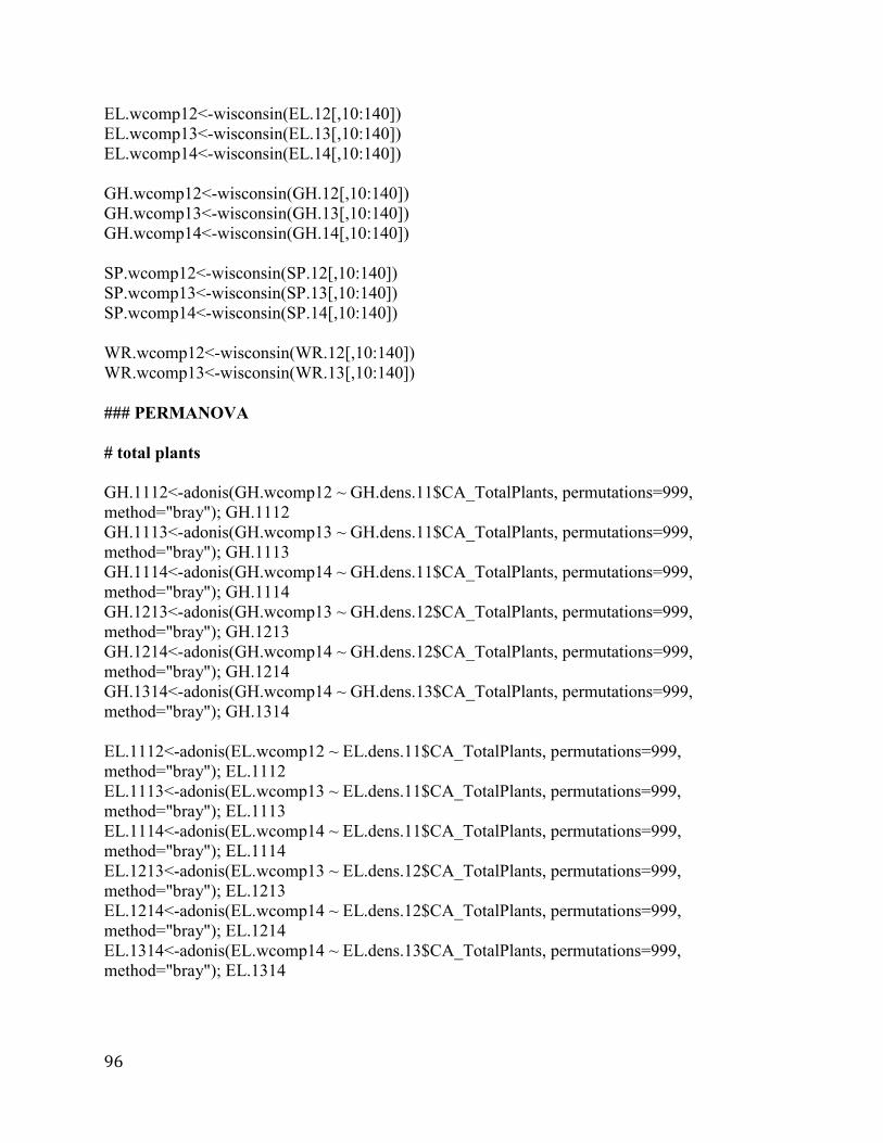
96

EL.wcomp12<-wisconsin(EL.12[,10:140])

EL.wcomp13<-wisconsin(EL.13[,10:140])

EL.wcomp14<-wisconsin(EL.14[,10:140])

GH.wcomp12<-wisconsin(GH.12[,10:140])

GH.wcomp13<-wisconsin(GH.13[,10:140])

GH.wcomp14<-wisconsin(GH.14[,10:140])

SP.wcomp12<-wisconsin(SP.12[,10:140])

SP.wcomp13<-wisconsin(SP.13[,10:140])

SP.wcomp14<-wisconsin(SP.14[,10:140])

WR.wcomp12<-wisconsin(WR.12[,10:140])

WR.wcomp13<-wisconsin(WR.13[,10:140])

### PERMANOVA

# total plants

GH.1112<-adonis(GH.wcomp12 ~ GH.dens.11$CA_TotalPlants, permutations=999,

method="bray"); GH.1112

GH.1113<-adonis(GH.wcomp13 ~ GH.dens.11$CA_TotalPlants, permutations=999,

method="bray"); GH.1113

GH.1114<-adonis(GH.wcomp14 ~ GH.dens.11$CA_TotalPlants, permutations=999,

method="bray"); GH.1114

GH.1213<-adonis(GH.wcomp13 ~ GH.dens.12$CA_TotalPlants, permutations=999,

method="bray"); GH.1213

GH.1214<-adonis(GH.wcomp14 ~ GH.dens.12$CA_TotalPlants, permutations=999,

method="bray"); GH.1214

GH.1314<-adonis(GH.wcomp14 ~ GH.dens.13$CA_TotalPlants, permutations=999,

method="bray"); GH.1314

EL.1112<-adonis(EL.wcomp12 ~ EL.dens.11$CA_TotalPlants, permutations=999,

method="bray"); EL.1112

EL.1113<-adonis(EL.wcomp13 ~ EL.dens.11$CA_TotalPlants, permutations=999,

method="bray"); EL.1113

EL.1114<-adonis(EL.wcomp14 ~ EL.dens.11$CA_TotalPlants, permutations=999,

method="bray"); EL.1114

EL.1213<-adonis(EL.wcomp13 ~ EL.dens.12$CA_TotalPlants, permutations=999,

method="bray"); EL.1213

EL.1214<-adonis(EL.wcomp14 ~ EL.dens.12$CA_TotalPlants, permutations=999,

method="bray"); EL.1214

EL.1314<-adonis(EL.wcomp14 ~ EL.dens.13$CA_TotalPlants, permutations=999,

method="bray"); EL.1314

97

SP.1112<-adonis(SP.wcomp12 ~ SP.dens.11$CA_TotalPlants, permutations=999,

method="bray"); SP.1112

SP.1113<-adonis(SP.wcomp13 ~ SP.dens.11$CA_TotalPlants, permutations=999,

method="bray"); SP.1113

SP.1114<-adonis(SP.wcomp14 ~ SP.dens.11$CA_TotalPlants, permutations=999,

method="bray"); SP.1114

SP.1213<-adonis(SP.wcomp13 ~ SP.dens.12$CA_TotalPlants, permutations=999,

method="bray"); SP.1213

SP.1214<-adonis(SP.wcomp14 ~ SP.dens.12$CA_TotalPlants, permutations=999,

method="bray"); SP.1214

SP.1314<-adonis(SP.wcomp14 ~ SP.dens.13$CA_TotalPlants, permutations=999,

method="bray"); SP.1314

WR.1112<-adonis(WR.wcomp12 ~ WR.dens.11$CA_TotalPlants, permutations=999,

method="bray"); WR.1112

WR.1113<-adonis(WR.wcomp13 ~ WR.dens.11$CA_TotalPlants, permutations=999,

method="bray"); WR.1113

WR.1213<-adonis(WR.wcomp13 ~ WR.dens.12$CA_TotalPlants, permutations=999,

method="bray"); WR.1213

### Richness

GH.rich1112<-adonis(GH.dens.11$Rich12 ~ GH.dens.11$CA_TotalPlants, permutations=999,

method="euc"); GH.rich1112

GH.rich1113<-adonis(GH.dens.11$Rich13 ~ GH.dens.11$CA_TotalPlants, permutations=999,

method="euc"); GH.rich1113

GH.rich1114<-adonis(GH.dens.11$Rich14 ~ GH.dens.11$CA_TotalPlants, permutations=999,

method="euc"); GH.rich1114

GH.rich1213<-adonis(GH.dens.12$Rich13 ~ GH.dens.12$CA_TotalPlants, permutations=999,

method="euc"); GH.rich1213

GH.rich1214<-adonis(GH.dens.12$Rich14 ~ GH.dens.12$CA_TotalPlants, permutations=999,

method="euc"); GH.rich1214

GH.rich1314<-adonis(GH.dens.13$Rich14 ~ GH.dens.13$CA_TotalPlants, permutations=999,

method="euc"); GH.rich1314

EL.rich1112<-adonis(EL.dens.11$Rich12 ~ EL.dens.11$CA_TotalPlants, permutations=999,

method="euc"); EL.rich1112

EL.rich1113<-adonis(EL.dens.11$Rich13 ~ EL.dens.11$CA_TotalPlants, permutations=999,

method="euc"); EL.rich1113

EL.rich1114<-adonis(EL.dens.11$Rich14 ~ EL.dens.11$CA_TotalPlants, permutations=999,

method="euc"); EL.rich1114

EL.rich1213<-adonis(EL.dens.12$Rich13 ~ EL.dens.12$CA_TotalPlants, permutations=999,

method="euc"); EL.rich1213

EL.rich1214<-adonis(EL.dens.12$Rich14 ~ EL.dens.12$CA_TotalPlants, permutations=999,

method="euc"); EL.rich1214

98

EL.rich1314<-adonis(EL.dens.13$Rich14 ~ EL.dens.13$CA_TotalPlants, permutations=999,

method="euc"); EL.rich1314

SP.rich1112<-adonis(SP.dens.11$Rich12 ~ SP.dens.11$CA_TotalPlants, permutations=999,

method="euc"); SP.rich1112

SP.rich1113<-adonis(SP.dens.11$Rich13 ~ SP.dens.11$CA_TotalPlants, permutations=999,

method="euc"); SP.rich1113

SP.rich1114<-adonis(SP.dens.11$Rich14 ~ SP.dens.11$CA_TotalPlants, permutations=999,

method="euc"); SP.rich1114

SP.rich1213<-adonis(SP.dens.12$Rich13 ~ SP.dens.12$CA_TotalPlants, permutations=999,

method="euc"); SP.rich1213

SP.rich1214<-adonis(SP.dens.12$Rich14 ~ SP.dens.12$CA_TotalPlants, permutations=999,

method="euc"); SP.rich1214

SP.rich1314<-adonis(SP.dens.13$Rich14 ~ SP.dens.13$CA_TotalPlants, permutations=999,

method="euc"); SP.rich1314

WR.rich1112<-adonis(WR.dens.11$Rich12 ~ WR.dens.11$CA_TotalPlants, permutations=999,

method="euc"); WR.rich1112

WR.rich1113<-adonis(WR.dens.11$Rich13 ~ WR.dens.11$CA_TotalPlants, permutations=999,

method="euc"); WR.rich1113

WR.rich1213<-adonis(WR.dens.12$Rich13 ~ WR.dens.12$CA_TotalPlants, permutations=999,

method="euc"); WR.rich1213

### Graphs

# Ordisurf

par(mfrow=c(1,1))

EL.test12<-metaMDS(EL.wcomp12, autotransform=FALSE, wascores=FALSE, distance =

“bray”, k = 2, trymax = 100)

EL.test13<-metaMDS(EL.wcomp13, autotransform=FALSE, wascores=FALSE, distance =

“bray”, k = 2, trymax = 100)

EL.test14<-metaMDS(EL.wcomp14, autotransform=FALSE, wascores=FALSE, distance =

“bray”, k = 2, trymax = 100)

GH.test12<-metaMDS(GH.wcomp12, autotransform=FALSE, wascores=FALSE, distance =

“bray”, k = 2, trymax = 100)

SP.test12<-metaMDS(SP.wcomp12, autotransform=FALSE, wascores=FALSE, distance =

“bray”, k = 2, trymax = 100)

WR.test12<-metaMDS(WR.wcomp12, autotransform=FALSE, wascores=FALSE, distance =

“bray”, k = 2, trymax = 100)

99

ordisurf(EL.test12, EL.dens.11$CA_TotalPlants, bubble=6, xlab="", xaxt="n", ylab="",

yaxt="n", main = "Ebey's Landing")

ordisurf(GH.test12, GH.dens.11$CA_TotalPlants, bubble=6, xlab="", xaxt="n", ylab="",

yaxt="n", main = "Glacial Heritage")

ordisurf(SP.test12, SP.dens.11$CA_TotalPlants, bubble=6, xlab="", xaxt="n", ylab="",

yaxt="n", main = "Smith Prairie")

ordisurf(WR.test12, WR.dens.11$CA_TotalPlants, bubble=6, xlab="", xaxt="n", ylab="",

yaxt="n", main = "West Rocky")

ordisurf(EL.test13, EL.dens.11$CA_TotalPlants, bubble=6, xlab="", xaxt="n", ylab="",

yaxt="n", main = "CALE density 11 x comm 2013")

ordisurf(EL.test14, EL.dens.11$CA_TotalPlants, bubble=6, xlab="", xaxt="n", ylab="",

yaxt="n", main = "CALE density 11 x comm 2014")

ordisurf(EL.test13, EL.dens.12$CA_TotalPlants, bubble=6, xlab="", xaxt="n", ylab="",

yaxt="n", main = "CALE density 12 x comm 2013")

# R2 vs median plant density

R2.plot<-read.csv(file.choose(), header=TRUE)

R2.plot$Site<-as.factor(R2.plot$Site)

# First try years between sampling just for fun

par(mfrow=c(1,2))

plot(R2.plot$Year.Diff, R2.plot$prop.rich, type="p", col="white", xlim = c(0.5,4), xlab="Year

difference", ylab="Variation from plant density")

points(jitter(R2.plot$Year.Diff[R2.plot$Site=="EL"]), R2.plot$prop.rich[R2.plot$Site=="EL"],

col="green", pch=17)

points(jitter(R2.plot$Year.Diff[R2.plot$Site=="GH"]), R2.plot$prop.rich[R2.plot$Site=="GH"],

col="orange", pch=1)

points(jitter(R2.plot$Year.Diff[R2.plot$Site=="SP"]), R2.plot$prop.rich[R2.plot$Site=="SP"],

col="red", pch=19)

points(jitter(R2.plot$Year.Diff[R2.plot$Site=="WR"]),

R2.plot$prop.rich[R2.plot$Site=="WR"], col="blue", pch=2)

legend(x="topright", pch=c(17, 1, 19, 2), legend = c("EL", "GH", "SP", "WR"), col=c("green",

"orange", "red", "blue"))

plot(R2.plot$Year.Diff, R2.plot$prop.comp, type="p", col="white", xlim = c(0.5,4), xlab="Year

difference", ylab = "")

points(jitter(R2.plot$Year.Diff[R2.plot$Site=="EL"]), R2.plot$prop.comp[R2.plot$Site=="EL"],

col="green", pch=17)

points(jitter(R2.plot$Year.Diff[R2.plot$Site=="GH"]),

R2.plot$prop.comp[R2.plot$Site=="GH"], col="orange", pch=1)

100

points(jitter(R2.plot$Year.Diff[R2.plot$Site=="SP"]), R2.plot$prop.comp[R2.plot$Site=="SP"],

col="red", pch=19)

points(jitter(R2.plot$Year.Diff[R2.plot$Site=="WR"]),

R2.plot$prop.comp[R2.plot$Site=="WR"], col="blue", pch=2)

legend(x="topright", pch=c(17, 1, 19, 2), legend = c("EL", "GH", "SP", "WR"), col=c("green",

"orange", "red", "blue"))

par(mfrow=c(1,2))

# Now look at variation in richness compared to median density

plot(R2.plot$Med.plants, R2.plot$prop.rich, type="p", col="white", xlim = c(0.5,16),

xlab="Median plant density", ylab="R2 value")

points(R2.plot$Med.plants[R2.plot$Site=="EL"], R2.plot$prop.rich[R2.plot$Site=="EL"],

col="green", pch=17)

points(R2.plot$Med.plants[R2.plot$Site=="GH"], R2.plot$prop.rich[R2.plot$Site=="GH"],

col="orange", pch=1)

points(R2.plot$Med.plants[R2.plot$Site=="SP"], R2.plot$prop.rich[R2.plot$Site=="SP"],

col="red", pch=19)

points(R2.plot$Med.plants[R2.plot$Site=="WR"], R2.plot$prop.rich[R2.plot$Site=="WR"],

col="blue", pch=2)

legend(x="topright", pch=c(17, 1, 19, 2), legend = c("EL", "GH", "SP", "WR"), col=c("green",

"orange", "red", "blue"))

# And variation in composition compared to median density

plot(R2.plot$Med.plants, R2.plot$prop.comp, type="p", col="white", xlim = c(0.5,16),

xlab="Median plant density", ylab="")

points(R2.plot$Med.plants[R2.plot$Site=="EL"], R2.plot$prop.comp[R2.plot$Site=="EL"],

col="green", pch=17)

points(R2.plot$Med.plants[R2.plot$Site=="GH"], R2.plot$prop.comp[R2.plot$Site=="GH"],

col="orange", pch=1)

points(R2.plot$Med.plants[R2.plot$Site=="SP"], R2.plot$prop.comp[R2.plot$Site=="SP"],

col="red", pch=19)

points(R2.plot$Med.plants[R2.plot$Site=="WR"], R2.plot$prop.comp[R2.plot$Site=="WR"],

col="blue", pch=2)

legend(x="topright", pch=c(17, 1, 19, 2), legend = c("EL", "GH", "SP", "WR"), col=c("green",

"orange", "red", "blue"))

### Show density range in each site in each year

par(mfrow=c(1,1))

101

plot(CA_TotalPlants[density$SampleYear=="2011"] ~

SiteAbbrev[density$SampleYear=="2011"], data = density, xlab="Site", ylab="Plant density")

plot(CA_TotalPlants[density$SampleYear=="2012"] ~

SiteAbbrev[density$SampleYear=="2012"], data = density, xlab="Site", ylab="Plant density")

plot(CA_TotalPlants[density$SampleYear=="2013"] ~

SiteAbbrev[density$SampleYear=="2013"], data = density, xlab="Site", ylab="Plant density")

### density and richness

par(mfrow=c(2,2))

plot(Rich12 ~ CA_TotalPlants, data = EL.dens.11, xlab = "Castilleja density", ylab = "Species

richness", xlim = c(0, 25), ylim = c(10, 35))

plot(Rich12 ~ CA_TotalPlants, data = GH.dens.11, xlab = "Castilleja density", ylab = "Species

richness", xlim = c(0, 25), ylim = c(10, 35))

plot(Rich12 ~ CA_TotalPlants, data = SP.dens.11, xlab = "Castilleja density", ylab = "Species

richness", xlim = c(0, 25), ylim = c(10, 35))

plot(Rich12 ~ CA_TotalPlants, data = WR.dens.11, xlab = "Castilleja density", ylab = "Species

richness", xlim = c(0, 25), ylim = c(10, 35))

plot(Rich13 ~ CA_TotalPlants, data = EL.dens.11, xlab = "CALE density", ylab = "Species

richness")

plot(Rich13 ~ CA_TotalPlants, data = GH.dens.11, xlab = "CALE density", ylab = "Species

richness")

plot(Rich13 ~ CA_TotalPlants, data = SP.dens.11, xlab = "CALE density", ylab = "Species

richness")

plot(Rich13 ~ CA_TotalPlants, data = WR.dens.11, xlab = "CALE density", ylab = "Species

richness")

plot(Rich14 ~ CA_TotalPlants, data = EL.dens.11, xlab = "CALE density", ylab = "Species

richness")

plot(Rich14 ~ CA_TotalPlants, data = GH.dens.11, xlab = "CALE density", ylab = "Species

richness")

plot(Rich14 ~ CA_TotalPlants, data = SP.dens.11, xlab = "CALE density", ylab = "Species

richness")

plot(Rich13 ~ CA_TotalPlants, data = EL.dens.12, xlab = "CALE density", ylab = "Species

richness")

plot(Rich13 ~ CA_TotalPlants, data = GH.dens.12, xlab = "CALE density", ylab = "Species

richness")

plot(Rich13 ~ CA_TotalPlants, data = SP.dens.12, xlab = "CALE density", ylab = "Species

richness")

plot(Rich13 ~ CA_TotalPlants, data = WR.dens.12, xlab = "CALE density", ylab = "Species

richness")

plot(Rich14 ~ CA_TotalPlants, data = EL.dens.12, xlab = "CALE density", ylab = "Species

richness")

102

plot(Rich14 ~ CA_TotalPlants, data = GH.dens.12, xlab = "CALE density", ylab = "Species

richness")

plot(Rich14 ~ CA_TotalPlants, data = SP.dens.12, xlab = "CALE density", ylab = "Species

richness")

plot(Rich14 ~ CA_TotalPlants, data = EL.dens.13, xlab = "CALE density", ylab = "Species

richness")

plot(Rich14 ~ CA_TotalPlants, data = GH.dens.13, xlab = "CALE density", ylab = "Species

richness")

plot(Rich14 ~ CA_TotalPlants, data = SP.dens.13, xlab = "CALE density", ylab = "Species

richness")

plot(Rich14 ~ CA_TotalPlants, data = EL.dens.11, xlab = "CALE density 2011", ylab = "Species

richness 2014")

plot(Rich13 ~ CA_TotalPlants, data = EL.dens.12, xlab = "CALE density 2012", ylab = "Species

richness 2013")

plot(Rich14 ~ CA_TotalPlants, data = GH.dens.12, xlab = "CALE density 2012", ylab =

"Species richness 2014")

plot(Rich14 ~ CA_TotalPlants, data = GH.dens.13, xlab = "CALE density 2013", ylab =

"Species richness 2014")