pareto efficient taxation - ocw.mit.edu · pareto efficient income taxation. iván werning. mit....
TRANSCRIPT
Pareto Efficient Income Taxation
Iván Werning
MIT
April 2007
NBER Public Economics meeting
Pareto Efficient Income Taxation - p. 1

Introduction ❖ Introduction ❖ Motivation ❖ Contribution ❖ Results
Model
Main Results
Applications
Conclusions
Pareto Efficient Income Taxation - p. 2
Introduction
Q: Good shape for tax schedule ?

Introduction
Introduction ❖ Introduction ❖ Motivation ❖ Contribution ❖ Results
Model
Main Results
Applications
Conclusions
Pareto Efficient Income Taxation - p. 2
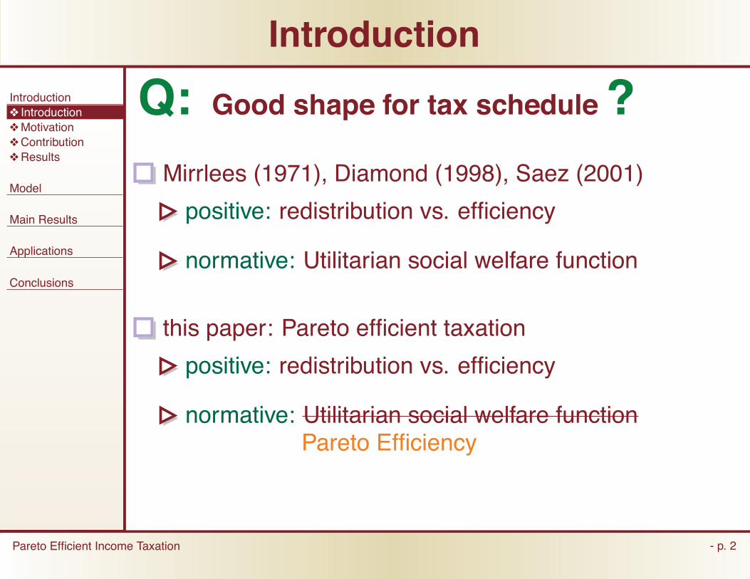
Q: Good shape for tax schedule ? Mirrlees (1971), Diamond (1998), Saez (2001)
positive: redistribution vs. efficiency
normative: Utilitarian social welfare function
Introduction ❖ Introduction ❖ Motivation ❖ Contribution ❖ Results
Model
Main Results
Applications
Conclusions
Pareto Efficient Income Taxation - p. 2
Introduction
Q: Good shape for tax schedule ? Mirrlees (1971), Diamond (1998), Saez (2001)
positive: redistribution vs. efficiency
normative: Utilitarian social welfare function
this paper: Pareto efficient taxation
positive: redistribution vs. efficiency
normative: Utilitarian social welfare function Pareto Efficiency

Introduction ❖ Introduction ❖ Motivation ❖ Contribution ❖ Results
Model
Main Results
Applications
Conclusions
Pareto Efficient Income Taxation - p. 3
Old Motivation: “New New New...”
Why not Utilitarian? (
i Ui)
practical: cardinality U i → W (U i) (or even W i(U i)) ... which Utilitarian?
conceptual: political process: social classes Coasian bargain ...but max
U i ?
philosophical: other notions of fairness and social justice

Introduction ❖ Introduction ❖ Motivation ❖ Contribution ❖ Results
Model
Main Results
Applications
Conclusions
Pareto Efficient Income Taxation - p. 3
Old Motivation: “New New New...”
Why not Utilitarian? ( i Ui)
practical: cardinality U i → W (U i) (or even W i(U i)) ... which Utilitarian?
conceptual: political process: social classes Coasian bargain ...but max U i ?
philosophical: other notions of fairness and social justice
Pareto efficiency weaker criterion
!
!

Introduction ❖ Introduction ❖ Motivation ❖ Contribution ❖ Results
Model
Main Results
Applications
Conclusions
Pareto Efficient Income Taxation - p. 4
Pareto Frontier
V�
VL
����������
�����������

Introduction ❖ Introduction ❖ Motivation ❖ Contribution ❖ Results
Model
Main Results
Applications
Conclusions
Pareto Efficient Income Taxation - p. 4
Pareto Frontier
V�
VL

Introduction ❖ Introduction ❖ Motivation ❖ Contribution ❖ Results
Model
Main Results
Applications
Conclusions
Pareto Efficient Income Taxation - p. 4
Pareto Frontier
V�
VL

Introduction ❖ Introduction ❖ Motivation ❖ Contribution ❖ Results
Model
Main Results
Applications
Conclusions
Pareto Efficient Income Taxation - p. 4
Pareto Frontier
V�
VL

Introduction ❖ Introduction ❖ Motivation ❖ Contribution ❖ Results
Model
Main Results
Applications
Conclusions
Pareto Efficient Income Taxation - p. 4
Pareto Frontier
V�
VL

Introduction ❖ Introduction ❖ Motivation ❖ Contribution ❖ Results
Model
Main Results
Applications
Conclusions
Pareto Efficient Income Taxation - p. 4
Pareto Frontier
V�
VL
�����L

Introduction ❖ Introduction ❖ Motivation ❖ Contribution ❖ Results
Model
Main Results
Applications
Conclusions
Pareto Efficient Income Taxation - p. 4
Pareto Frontier
V�
VL
�����L
Ȝ������ Ȝ���L

Introduction ❖ Introduction ❖ Motivation ❖ Contribution ❖ Results
Model
Main Results
Applications
Conclusions
Pareto Efficient Income Taxation - p. 5
Contribution
invert Mirrlees model...
...express in tractable way
...use it: some applications

Results
Introduction ❖ Introduction ❖ Motivation ❖ Contribution ❖ Results
Model
Main Results
Applications
Conclusions
Pareto Efficient Income Taxation - p. 6
#0 restrictions generalize “zero-tax-at-the-top” #1 Any T (Y ). . .
efficient for many f(θ)
inefficient for many f(θ) . . . anything goes
#2 Given T0(Y ) g(Y ) f(θ) (Saez, 2001) efficient set of T (Y ): large
inefficient set of T (Y ): large
#3 Simple test for efficiency of T0(Y )

Results
Introduction ❖ Introduction ❖ Motivation ❖ Contribution ❖ Results
Model
Main Results
Applications
Conclusions
Pareto Efficient Income Taxation - p. 7
#4 Simple formulas...
bound on top tax rate
efficiency of a flat tax
#5 Increasing progressivity maintains Pareto efficiency
#6 observable heterogeneity not conditioning can be efficient

Setup
Introduction
Model ❖ Setup ❖ Planning Problem ❖ Efficiency Conditions
Main Results
Applications
Conclusions
Pareto Efficient Income Taxation - p. 8
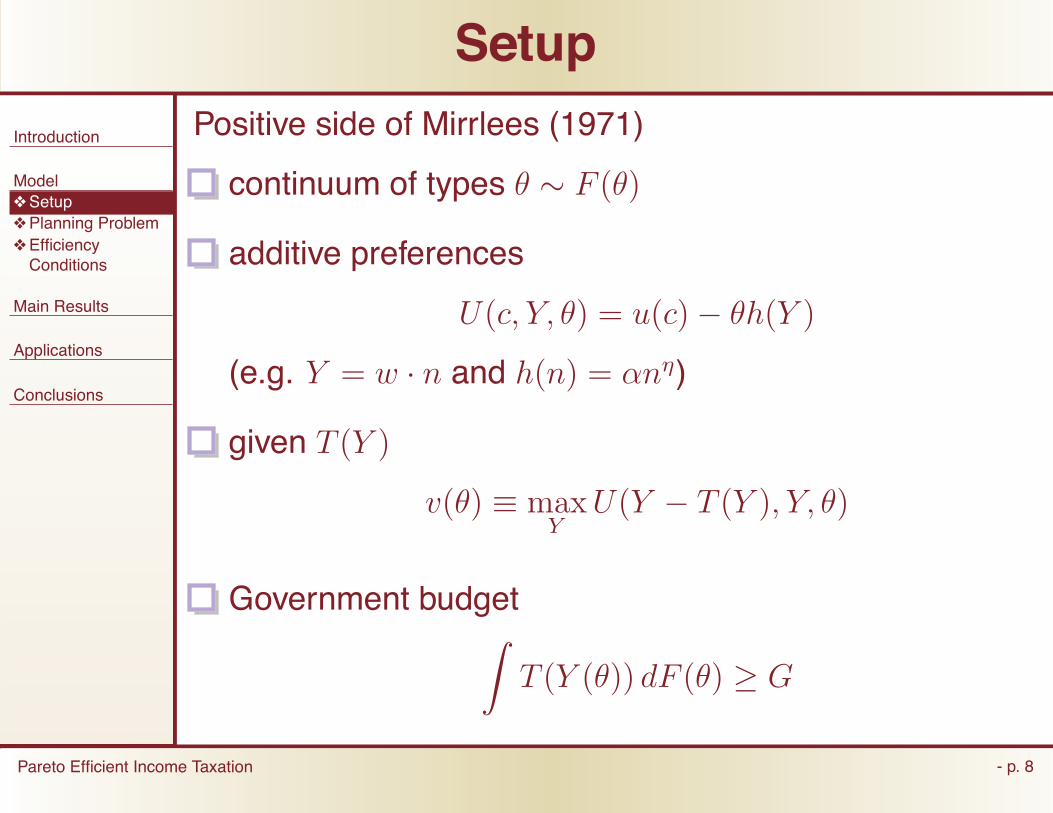
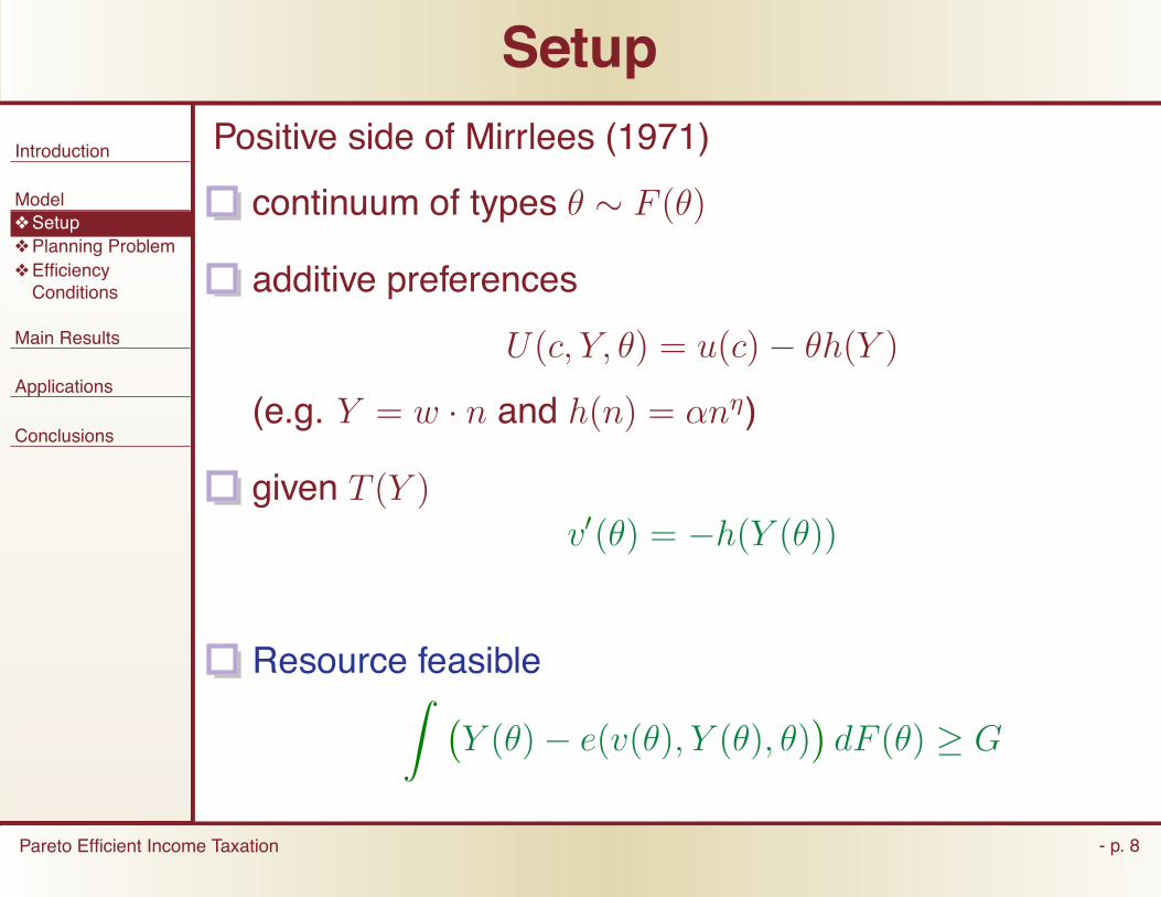
Positive side of Mirrlees (1971)
continuum of types θ ∼ F (θ)
additive preferences
U(c, Y, θ) = u(c) − θh(Y )
(e.g. Y = w · n and h(n) = αnη)

Setup
Introduction
Model ❖ Setup ❖ Planning Problem ❖ Efficiency Conditions
Main Results
Applications
Conclusions
Pareto Efficient Income Taxation - p. 8
Positive side of Mirrlees (1971)
continuum of types θ ∼ F (θ)
additive preferences
U(c, Y, θ) = u(c) − θh(Y )
(e.g. Y = w · n and h(n) = αnη)
given T (Y )
v(θ) ≡ max Y
U(Y − T (Y ), Y, θ)
Government budget � T (Y (θ)) dF (θ) ≥ G

�
Setup
Introduction
Model ❖ Setup ❖ Planning Problem ❖ Efficiency Conditions
Main Results
Applications
Conclusions
Pareto Efficient Income Taxation - p. 8
Positive side of Mirrlees (1971)
continuum of types θ ∼ F (θ)
additive preferences
U(c, Y, θ) = u(c) − θh(Y )
(e.g. Y = w · n and h(n) = αnη)
given T (Y )
v(θ) ≡ max Y
U(Y − T (Y ), Y, θ)
Resource feasible � Y (θ) − c(θ)
� dF (θ) ≥ G
"

� � �
Setup
Introduction
Model ❖ Setup ❖ Planning Problem ❖ Efficiency Conditions
Main Results
Applications
Conclusions
Pareto Efficient Income Taxation - p. 8
Positive side of Mirrlees (1971)
continuum of types θ ∼ F (θ)
additive preferences
U(c, Y, θ) = u(c) − θh(Y )
(e.g. Y = w · n and h(n) = αnη)
given T (Y )
v ′(θ) = Uθ(Y (θ) − T (Y (θ)), Y (θ), θ)
Resource feasible
Y (θ) − c(θ) dF (θ) ≥ G "
# $

′
� � �
Setup
Introduction
Model ❖ Setup ❖ Planning Problem ❖ Efficiency Conditions
Main Results
Applications
Conclusions
Pareto Efficient Income Taxation - p. 8
Positive side of Mirrlees (1971)
continuum of types θ ∼ F (θ)
additive preferences
U(c, Y, θ) = u(c) − θh(Y )
(e.g. Y = w · n and h(n) = αnη)
given T (Y ) v (θ) = −h(Y (θ))
Resource feasible
Y (θ) − c(θ) dF (θ) ≥ G $#
"
!
′
� � �
Setup
Introduction
Model ❖ Setup ❖ Planning Problem ❖ Efficiency Conditions
Main Results
Applications
Conclusions
Pareto Efficient Income Taxation - p. 8
Positive side of Mirrlees (1971)
continuum of types θ ∼ F (θ)
additive preferences
U(c, Y, θ) = u(c) − θh(Y )
(e.g. Y = w · n and h(n) = αnη)
given T (Y ) v (θ) = −h(Y (θ))
Resource feasible
Y (θ) − e(v(θ), Y (θ), θ) dF (θ) ≥ G "
# $
!

Introduction
Model ❖ Setup ❖ Planning Problem ❖ Efficiency Conditions
Main Results
Applications
Conclusions
Pareto Efficient Income Taxation - p. 9
Planning Problem
Dual Pareto Problem
maximize net resources
subject to, v(θ) ≥ v(θ)
incentives

� � �Introduction
Model ❖ Setup ❖ Planning Problem ❖ Efficiency Conditions
Main Results
Applications
Conclusions
Pareto Efficient Income Taxation - p. 9
Planning Problem
Dual Pareto Problem
max Y ,v
Y (θ) − e(v(θ), Y (θ), θ) dF (θ)
subject to, v(θ) ≥ v(θ)
incentives
"
# $

� � �
′
Introduction
Model ❖ Setup ❖ Planning Problem ❖ Efficiency Conditions
Main Results
Applications
Conclusions
Pareto Efficient Income Taxation - p. 9
Planning Problem
Dual Pareto Problem
max Y ,v
Y (θ) − e(v(θ), Y (θ), θ) dF (θ)
subject to, v(θ) ≥ v(θ)
v (θ) = −h( Y (θ))
$
"
#
!

� � �
′
Introduction
Model ❖ Setup ❖ Planning Problem ❖ Efficiency Conditions
Main Results
Applications
Conclusions
Pareto Efficient Income Taxation - p. 9
Planning Problem
Dual Pareto Problem
max Y ,v
Y (θ) − e(v(θ), Y (θ), θ) dF (θ)
subject to, v(θ) ≥ v(θ)
v (θ) = −h( Y (θ))
Y (θ) nonincreasing
#
"
$
!

� � ��
′
Introduction
Model ❖ Setup ❖ Planning Problem ❖ Efficiency Conditions
Main Results
Applications
Conclusions
Pareto Efficient Income Taxation - p. 10
Efficiency Conditions
Lagrangian
L = Y (θ)−e(v(θ), Y (θ), θ) dF (θ)
− � v (θ) + h( Y (θ))
� μ(θ) dθ
"
#
"
$
!

� � ��
′
�
Introduction
Model ❖ Setup ❖ Planning Problem ❖ Efficiency Conditions
Main Results
Applications
Conclusions
Pareto Efficient Income Taxation - p. 10
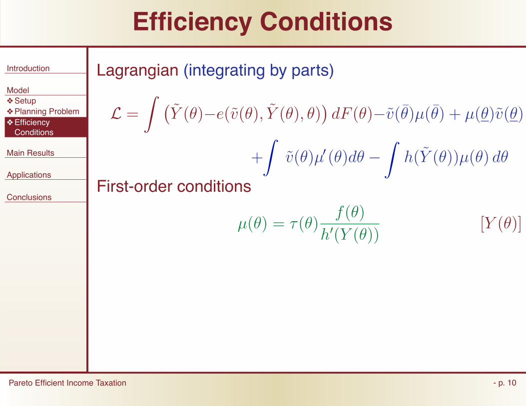
Efficiency Conditions
Lagrangian (integrating by parts)
L = Y (θ)−e(v(θ), Y (θ), θ) dF (θ)−v(θ)μ(θ) + μ(θ)v(θ)
+ v(θ)μ (θ)dθ − h( Y (θ))μ(θ) dθ
$
"
#
""
!

� � ��
′
�
� �′
Introduction
Model ❖ Setup ❖ Planning Problem ❖ Efficiency Conditions
Main Results
Applications
Conclusions
Pareto Efficient Income Taxation - p. 10
Efficiency Conditions
Lagrangian (integrating by parts)
L = Y (θ)−e(v(θ), Y (θ), θ) dF (θ)−v(θ)μ(θ) + μ(θ)v(θ)
+ v(θ)μ (θ)dθ − h( Y (θ))μ(θ) dθ
First-order conditions
1 − eY (v(θ), Y (θ), θ) f(θ) = μ(θ)h (Y (θ)) [Y (θ)]
""
$
$
"
#
#
!
!

� � ��
′
�
′
Introduction
Model ❖ Setup ❖ Planning Problem ❖ Efficiency Conditions
Main Results
Applications
Conclusions
Pareto Efficient Income Taxation - p. 10
Efficiency Conditions
Lagrangian (integrating by parts)
L = Y (θ)−e(v(θ), Y (θ), θ) dF (θ)−v(θ)μ(θ) + μ(θ)v(θ)
+ v(θ)μ (θ)dθ − h( Y (θ))μ(θ) dθ
First-order conditions
τ(θ)f(θ) = μ(θ)h (Y (θ)) [Y (θ)]
"
# $
""
!
!
� � ��
′
�
′
Introduction
Model ❖ Setup ❖ Planning Problem ❖ Efficiency Conditions
Main Results
Applications
Conclusions
Pareto Efficient Income Taxation - p. 10
Efficiency Conditions
Lagrangian (integrating by parts)
L = Y (θ)−e(v(θ), Y (θ), θ) dF (θ)−v(θ)μ(θ) + μ(θ)v(θ)
+ v(θ)μ (θ)dθ − h( Y (θ))μ(θ) dθ
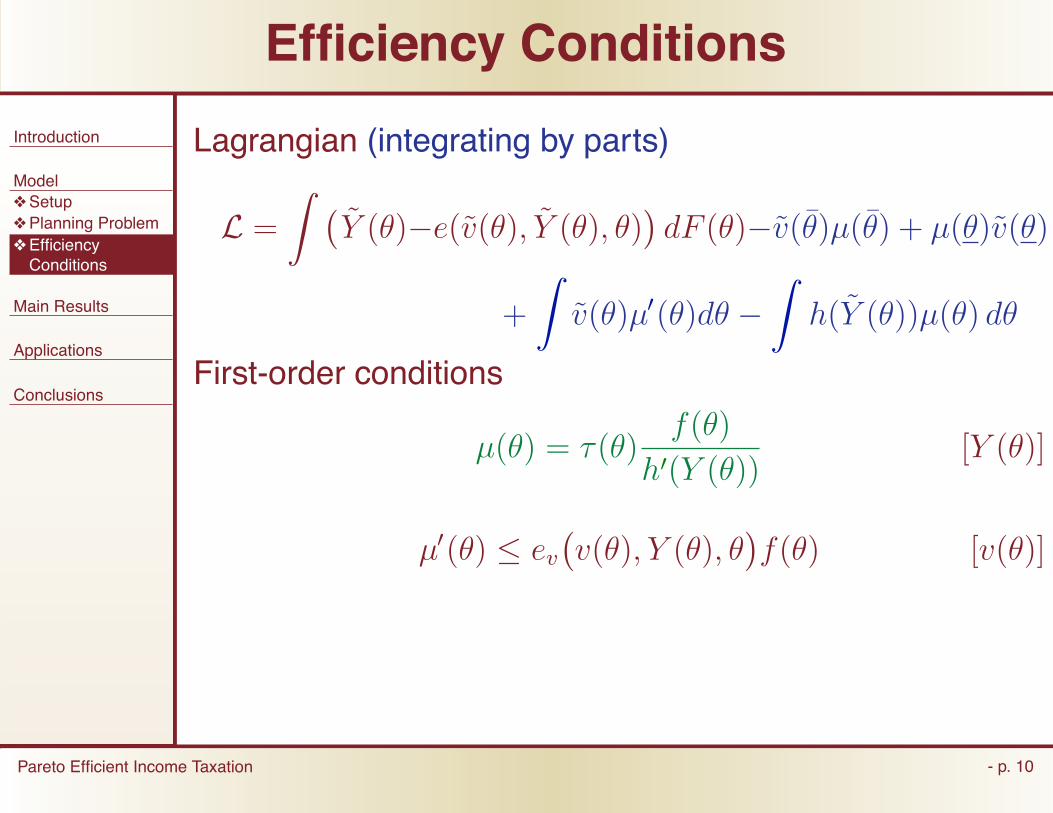
First-order conditions
μ(θ) = τ(θ) f(θ)
h (Y (θ)) [Y (θ)]
"
"
"
# $
!
!
� � ��
′
�
′
′� �
Introduction
Model ❖ Setup ❖ Planning Problem ❖ Efficiency Conditions
Main Results
Applications
Conclusions
Pareto Efficient Income Taxation - p. 10
Efficiency Conditions
Lagrangian (integrating by parts)
L = Y (θ)−e(v(θ), Y (θ), θ) dF (θ)−v(θ)μ(θ) + μ(θ)v(θ)
+ v(θ)μ (θ)dθ − h( Y (θ))μ(θ) dθ
First-order conditions
μ(θ) = τ(θ) f(θ)
h (Y (θ)) [Y (θ)]
μ (θ) ≤ ev v(θ), Y (θ), θ f(θ) [v(θ)]
$
""
"
#
$#
!
!
!

� � ��
′
�
′
′� �
′ ′
Introduction
Model ❖ Setup ❖ Planning Problem ❖ Efficiency Conditions
Main Results
Applications
Conclusions
Pareto Efficient Income Taxation - p. 10
Efficiency Conditions
Lagrangian (integrating by parts)
L = Y (θ)−e(v(θ), Y (θ), θ) dF (θ)−v(θ)μ(θ) + μ(θ)v(θ)
+ v(θ)μ (θ)dθ − h( Y (θ))μ(θ) dθ
First-order conditions
μ(θ) = τ(θ) f(θ)
h (Y (θ)) [Y (θ)]
μ (θ) ≤ ev v(θ), Y (θ), θ f(θ) [v(θ)]
τ(θ)
�
θ τ (θ) τ(θ)
+ d log f(θ)
d log θ −
d log h (Y (θ)) d log θ
�
≤ 1 − τ (θ)
#
"
# $
$
"
"
!
!
! !

�′ ′
Introduction
Model
Main Results ❖ Intuition ❖ Anything Goes ❖ Identification and Test
❖ Graphical Test ❖ Empirical Strategy ❖ Quantifying Inefficiencies
Applications
Conclusions
Pareto Efficient Income Taxation - p. 11
Efficiency Conditions
Proposition. T (Y ) is Pareto efficient if and only
τ(θ) θ τ (θ) τ (θ)
+ d log f(θ)
d log θ −
d log h (Y (θ)) d log θ
�
≤ 1 − τ(θ)
τ(θ) ≥ 0 and τ(θ) ≤ 0.
'
! !

�′ ′
Introduction
Model
Main Results ❖ Intuition ❖ Anything Goes ❖ Identification and Test
❖ Graphical Test ❖ Empirical Strategy ❖ Quantifying Inefficiencies
Applications
Conclusions
Pareto Efficient Income Taxation - p. 11
Efficiency Conditions
Proposition. T (Y ) is Pareto efficient if and only
τ(θ) θ τ (θ) τ (θ)
+ d log f(θ)
d log θ −
d log h (Y (θ)) d log θ
�
≤ 1 − τ(θ)
τ(θ) ≥ 0 and τ(θ) ≤ 0.
note: “zero-tax-at-top” special case
'
! !

�′ ′
′
�′
Introduction
Model
Main Results ❖ Intuition ❖ Anything Goes ❖ Identification and Test
❖ Graphical Test ❖ Empirical Strategy ❖ Quantifying Inefficiencies
Applications
Conclusions
Pareto Efficient Income Taxation - p. 11
Efficiency Conditions
Proposition. T (Y ) is Pareto efficient if and only
τ(θ) θ τ (θ) τ (θ)
+ d log f(θ)
d log θ −
d log h (Y (θ)) d log θ
�
≤ 1 − τ(θ)
τ(θ) ≥ 0 and τ(θ) ≤ 0.
note: “zero-tax-at-top” special case
more general condition:
τ (θ)f(θ) h (Y (θ))
+ θ
θ
1
u (c(θ)) f(θ) dθ is nonincreasing
'
"
! !
! !

�′ ′
Intuition
Introduction
Model
Main Results ❖ Intuition ❖ Anything Goes ❖ Identification and Test
❖ Graphical Test ❖ Empirical Strategy ❖ Quantifying Inefficiencies
Applications
Conclusions
Pareto Efficient Income Taxation - p. 12
define
T (Y ) ≡
T (Y (θ)) − ε Y = Y (θ)
T (Y ) Y = Y (θ)
Proposition. T > T
τ(θ) θ τ (θ) τ(θ)
+ 2 d log f(θ)
d log θ −
d log h (Y (θ)) d log θ
�
≤ 3(1 − τ(θ))
is violated at θ
'
! !

Introduction
Model
Main Results ❖ Intuition ❖ Anything Goes ❖ Identification and Test
❖ Graphical Test ❖ Empirical Strategy ❖ Quantifying Inefficiencies
Applications
Conclusions
Pareto Efficient Income Taxation - p. 13
Simple Tax Reform
Y
T

Introduction
Model
Main Results ❖ Intuition ❖ Anything Goes ❖ Identification and Test
❖ Graphical Test ❖ Empirical Strategy ❖ Quantifying Inefficiencies
Applications
Conclusions
Pareto Efficient Income Taxation - p. 13
Simple Tax Reform
Y
T

Introduction
Model
Main Results ❖ Intuition ❖ Anything Goes ❖ Identification and Test
❖ Graphical Test ❖ Empirical Strategy ❖ Quantifying Inefficiencies
Applications
Conclusions
Pareto Efficient Income Taxation - p. 13
Simple Tax Reform
Y
T

Introduction
Model
Main Results ❖ Intuition ❖ Anything Goes ❖ Identification and Test
❖ Graphical Test ❖ Empirical Strategy ❖ Quantifying Inefficiencies
Applications
Conclusions
Pareto Efficient Income Taxation - p. 13
Simple Tax Reform
Y
T

Introduction
Model
Main Results ❖ Intuition ❖ Anything Goes ❖ Identification and Test
❖ Graphical Test ❖ Empirical Strategy ❖ Quantifying Inefficiencies
Applications
Conclusions
Pareto Efficient Income Taxation - p. 13
Simple Tax Reform
Y
T
Introduction
Model
Main Results ❖ Intuition ❖ Anything Goes ❖ Identification and Test
❖ Graphical Test ❖ Empirical Strategy ❖ Quantifying Inefficiencies
Applications
Conclusions
Pareto Efficient Income Taxation - p. 13
Simple Tax Reform
Y
T
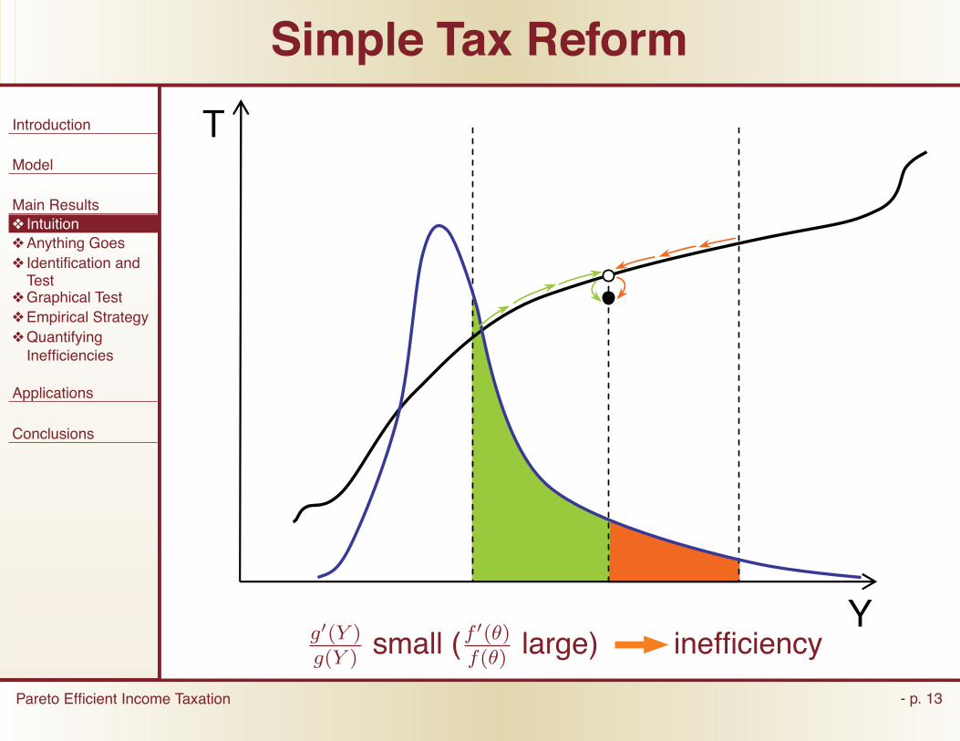
g'(Y ) g(Y ) small (
f '(θ) f(θ) large) inefficiency

Laffer
Introduction
Model
Main Results ❖ Intuition ❖ Anything Goes ❖ Identification and Test
❖ Graphical Test ❖ Empirical Strategy ❖ Quantifying Inefficiencies
Applications
Conclusions
Pareto Efficient Income Taxation - p. 14
lower taxes increase revenue
Pareto improvements “Laffer” effect
Proposition. T1(Y ) > T0(Y ) T1(Y ) ≤ T0(Y )

�′ ′
Introduction
Model
Main Results ❖ Intuition ❖ Anything Goes ❖ Identification and Test
❖ Graphical Test ❖ Empirical Strategy ❖ Quantifying Inefficiencies
Applications
Conclusions
Pareto Efficient Income Taxation - p. 15
Anything Goes
τ(θ) θ τ (θ) τ(θ)
+ d log f(θ)
d log θ −
d log h (Y (θ)) d log θ
�
≤ 1 − τ (θ)
Proposition. For any T (Y )
exists set {f(θ)} Pareto efficient
exists set {f(θ)} Pareto inefficient
'
! !

�′ ′
Introduction
Model
Main Results ❖ Intuition ❖ Anything Goes ❖ Identification and Test
❖ Graphical Test ❖ Empirical Strategy ❖ Quantifying Inefficiencies
Applications
Conclusions
Pareto Efficient Income Taxation - p. 15
Anything Goes
τ(θ) θ τ (θ) τ(θ)
+ d log f(θ)
d log θ −
d log h (Y (θ)) d log θ
�
≤ 1 − τ (θ)
Proposition. For any T (Y )
exists set {f(θ)} Pareto efficient
exists set {f(θ)} Pareto inefficient
without empirical knowledge anything goes
need information on f(θ) to restrict T (Y )
'
! !

′
′
′
′
Introduction
Model
Main Results ❖ Intuition ❖ Anything Goes ❖ Identification and Test
❖ Graphical Test ❖ Empirical Strategy ❖ Quantifying Inefficiencies
Applications
Conclusions
Pareto Efficient Income Taxation - p. 16
Identification and Test
observe g(Y ) identify (Saez, 2001)
θ(Y ) = (1 − T (Y )) u (Y − T (Y ))
h (Y )
f(θ(Y )) = g(Y ) θ (Y )
!
!
!
!

′
′
′
′
Introduction
Model
Main Results ❖ Intuition ❖ Anything Goes ❖ Identification and Test
❖ Graphical Test ❖ Empirical Strategy ❖ Quantifying Inefficiencies
Applications
Conclusions
Pareto Efficient Income Taxation - p. 16
Identification and Test
observe g(Y ) identify (Saez, 2001)
θ(Y ) = (1 − T (Y )) u (Y − T (Y ))
h (Y )
f(θ(Y )) = g(Y ) θ (Y )
efficiency test...
d log g(Y ) d log Y
≥ a(Y )
... for tax schedule in place
!
!
!

��
Introduction
Model
Main Results ❖ Intuition ❖ Anything Goes ❖ Identification and Test
❖ Graphical Test ❖ Empirical Strategy ❖ Quantifying Inefficiencies
Applications
Conclusions
Pareto Efficient Income Taxation - p. 17
Graphical Test
define Rawlsian density:
α(Y ) = exp
Y 0 a(z) dz
�
∞ 0 exp
Y 0 a(z) dz
�
graphical test:
g(Y ) α(Y )
nondecreasing
0.5 1 1.5 2 2.5 3 3.5 4 4.5 5 5.5 6 0
0.05
0.1
0.15
0.2
0.25
0.3
%
%

Introduction
Model
Main Results ❖ Intuition ❖ Anything Goes ❖ Identification and Test
❖ Graphical Test ❖ Empirical Strategy ❖ Quantifying Inefficiencies
Applications
Conclusions
Pareto Efficient Income Taxation - p. 18
Empirical Implementation
needed 1. current tax function T (Y )
2. distribution of income g(Y )
3. utility function U(c, Y, θ)
in principle: #1 and #2 easy #3 usual deal
Diamond (1998) and Saez (2001)

′
Introduction
Model
Main Results ❖ Intuition ❖ Anything Goes ❖ Identification and Test
❖ Graphical Test ❖ Empirical Strategy ❖ Quantifying Inefficiencies
Applications
Conclusions
Pareto Efficient Income Taxation - p. 18
Empirical Implementation
needed 1. current tax function T (Y )
2. distribution of income g(Y )
3. utility function U(c, Y, θ)
in principle: #1 and #2 easy #3 usual deal
Diamond (1998) and Saez (2001)
some challenges... 1. econometric: need to estimate g (Y ) and g(Y )
2. conceptual: static model lifetime T (Y ) and g(Y ) (Fullerton and Rogers)
!

Introduction
Model
Main Results ❖ Intuition ❖ Anything Goes ❖ Identification and Test
❖ Graphical Test ❖ Empirical Strategy ❖ Quantifying Inefficiencies
Applications
Conclusions
Pareto Efficient Income Taxation - p. 19
Output Density
IRS’s SOI Public Use Files for Individual tax returns
lifetime g(Y )?
lifetime T (Y ) schedule?
Y i = 1 n Y i t
smooth density estimate assumed T (Y ) = .30 × Y
!

( )
Introduction
Model
Main Results ❖ Intuition ❖ Anything Goes ❖ Identification and Test
❖ Graphical Test ❖ Empirical Strategy ❖ Quantifying Inefficiencies
Applications
Conclusions
Pareto Efficient Income Taxation - p. 19
Output Density
IRS’s SOI Public Use Files for Individual tax returns
lifetime g(Y )?
lifetime T (Y ) schedule?
Y i = 1 n Y i t
smooth density estimate assumed T (Y ) = .30 × Y
0 0.5 1 1.5 2 2.5
x 105
0
0.2
0.4
0.6
0.8
1
1.2
1.4
1.6
1.8
2 x 10
−5
Average Income (in 1990 dollars)
nsity (bandwidth = 10,000) of Average Income Over Varying Time Periods in the Un
>= 10 years during 1979−1990 1982−1986 1987−1990
Figure 1: Density of income
g(Y )
0 2 4 6 8 10 12 14 16 18
x 104
−12
−10
−8
−6
−4
−2
0
2
Average Income (in 1990 dollars)
ernel Density (bandwidth = 10,000) of Average Income Over Varying Time Periods in
>= 10 years during 1979−199 1982−1986 1987−1990
Figure 2: Implied elasticity Y g'(Y )
!

Introduction
Model
Main Results ❖ Intuition ❖ Anything Goes ❖ Identification and Test
❖ Graphical Test ❖ Empirical Strategy ❖ Quantifying Inefficiencies
Applications
Conclusions
Pareto Efficient Income Taxation - p. 19
Output Density
IRS’s SOI Public Use Files for Individual tax returns
lifetime g(Y )?
lifetime T (Y ) schedule?
Y i = 1 n Y i t
smooth density estimate assumed T (Y ) = .30 × Y
0 2 4 6 8 10
x 104
0
0.5
1
1.5
2
2.5
3
x 10−5Rawlsian Test against 1987−1990 Average Income Data (sigma = 0, eta = 2, T = .3
0 1 2 3 4 5 6 7 8 9 10
x 104
0
1
2
3
4
5
x 10−5Rawlsian Test against 1987−1990 Average Income Data (sigma = 1, eta = 3, T = .3Y
!

� � � � � �Introduction
Model
Main Results ❖ Intuition ❖ Anything Goes ❖ Identification and Test
❖ Graphical Test ❖ Empirical Strategy ❖ Quantifying Inefficiencies
Applications
Conclusions
Pareto Efficient Income Taxation - p. 20
Quantifying Inefficiencies
efficiency test qualitative
quantitative. . .
Δ ≡ Y ∗(θ) − c ∗(θ) dF (θ) − Y (θ) − c(θ) dF (θ)
does not count welfare improvements
v(θ) > v(θ)
"
#
"
#

′
Introduction
Model
Main Results
Applications ❖ Top Tax Rate ❖ Flat Tax ❖ Progressivity ❖ Heterogeneity
Conclusions
Pareto Efficient Income Taxation - p. 21
Top Tax Rate
u(c) = c1−σ/(1 − σ) and h(Y ) = αY η
suppose top tax rate
τ ≡ lim θ→0
τ(θ) = lim Y →∞
T (Y )
exists
!

′
Introduction
Model
Main Results
Applications ❖ Top Tax Rate ❖ Flat Tax ❖ Progressivity ❖ Heterogeneity
Conclusions
Pareto Efficient Income Taxation - p. 21
Top Tax Rate
u(c) = c1−σ/(1 − σ) and h(Y ) = αY η
suppose top tax rate
τ ≡ lim θ→0
τ(θ) = lim Y →∞
T (Y )
exists
efficiency condition bound
τ ≤ σ + η − 1 ϕ + η − 2
.
where ϕ = − limT →∞ d log g(Y )/d log Y .
Saez (2001): ϕ = 3
!

Top Tax Rate 1
Introduction
0.9Model
Main Results 0.8
Applications ❖ Top Tax Rate 0.7
❖ Flat Tax ❖ Progressivity
0.6 ❖ Heterogeneity
Conclusions 0.5
0.4
0.3
0.2
0.1
0 0 1 2 3 4 5 6 7 8 9
elasticity 1/η+1
upper bound on τ
Pareto Efficient Income Taxation - p. 22
10

Flat Tax
Introduction
Model
Main Results
Applications ❖ Top Tax Rate ❖ Flat Tax ❖ Progressivity ❖ Heterogeneity
Conclusions
Pareto Efficient Income Taxation - p. 23
linear tax necessary condition
τ ≤ σ + η − 1
−d log g(Y ) d log Y + η − 2
linear tax sufficient condition
τ ≤ η − 1
−d log g(Y ) d log Y + η − 1

Introduction
Model
Main Results
Applications ❖ Top Tax Rate ❖ Flat Tax ❖ Progressivity ❖ Heterogeneity
Conclusions
Pareto Efficient Income Taxation - p. 24
Progressivity
Quasi-linear u(c) = c
result: can always increase progressivity

Introduction
Model
Main Results
Applications ❖ Top Tax Rate ❖ Flat Tax ❖ Progressivity ❖ Heterogeneity
Conclusions
Pareto Efficient Income Taxation - p. 25
Heterogeneity
groups = 1, . . . , N
f i(θ) and U i(c, Y, θ)
unobservable i single T (Y )
average efficiency condition
observable i multiple T i(Y )
N efficiency conditions
observation: T i(Y ) = T (Y ) may be Pareto efficient
never optimal for Utilitarian

Conclusions
Introduction
Model
Main Results
Applications
Conclusions ❖ Conclusions
Pareto Efficient Income Taxation - p. 26
Pareto efficiency simple condition
generalizes zero-tax-at-the-top result
Pareto inefficient Laffer effects
flat taxes may be optimal...
...more progressivity always efficient

��������� ���� �������������������
���������� ���!���������"� �#$�#
"� ��%� ����������������&����������� �� ��� ��� ��� ����%�'��(�)��������������������������� ���