parra lab - bme 50500: image and signal …1 lucas parra, ccny city college of new york bme 50500:...

1

Lucas Parra, CCNY City College of New York

BME 50500: Image and Signal Processing in Biomedicine

Lecture 2: Discrete Fourier Transform

Lucas C. ParraBiomedical Engineering DepartmentCity College of New York

CCNY

2


Complex Numbers

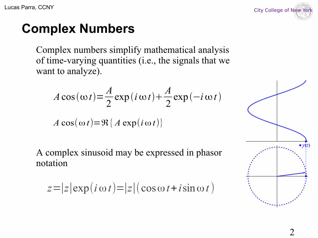
Complex numbers simplify mathematical analysis of time-varying quantities (i.e., the signals that we want to analyze).

A complex sinusoid may be expressed in phasor notation

A cos t =A2

exp i t A2

exp −i t

A cos(ω t)=ℜ{A exp(i ω t)}

z=∣z∣exp(i ω t)=∣z∣(cosω t+ isinω t )

3


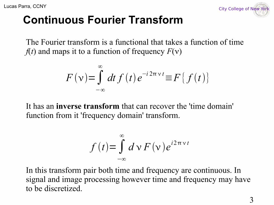
The Fourier transform is a functional that takes a function of time f(t) and maps it to a function of frequency F()

It has an inverse transform that can recover the 'time domain' function from it 'frequency domain' transform.

In this transform pair both time and frequency are continuous. In signal and image processing however time and frequency may have to be discretized.

Continuous Fourier Transform

F =∫−∞

∞

dt f t e−i 2 t≡F { f t }

f t =∫−∞

∞

d F e i 2 t

4



f (t) |F ()|

t

By Lucas V. Barbosa https://commons.wikimedia.org/w/index.php?curid=24830373

5


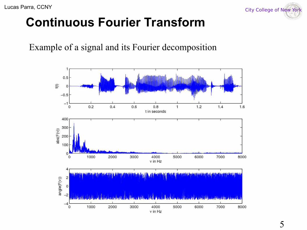
Example of a signal and its Fourier decomposition


F =∫−∞

∞

dt f t e−i 2 t≡F { f t }

f t =∫−∞

∞

d F e i 2 t

6


Examples

CFT - Examples

FT {cos 2 ot }=12

−o o

FT {1}=

FT {t−t o}=e−2 i t o

FT {e−a t 2

}=

ae−

2

2/ a

FT {rect t }=sinc=sin

rect t ={1 ∣t∣1/2

0 else }

7


'Stretching' time 'shrinks' frequency and vise versa

CFT – Scale Theorem

FT { f a t }=1a

FT

a

t

Shortpulse

Medium-lengthpulse

Longpulse

The shorter the pulse,

the broader the spectrum!

This is the essence of the Uncertainty Principle!

t

t

f(t)

F()

8


(1) From the definition:

(2) It then follows that:

(3) Change of variables

(4) Substituting into the integral:

f (t )=∫−∞

∞

F()e i2 π t d

f (at)=∫−∞

∞

F()e i 2π at d

f (at)=∫−∞

∞ 1a

F ( ωa

)ei 2π ωt dω

ω= a d ω=a d

FT {f (at)}=1a

FT { a

}

CFT – Scale Theorem derivation

9


There is a tradeoff between temporal extend and frequency bandwidth. There is a lower bound on the time-bandwidth product

● A signal that has a well defined frequency must be extended in time.● A short signal must be broadband.

CFT – Uncertainty Principle

t

f(t) F()

t

t2=

1B∫dt∣ f t ∣

2t 2

2=

1B∫d ∣ F ∣

2

2

B=∫ d ∣F ∣2=∫ dt∣ f t ∣

2

t ≥12

Fourier Transform

10


The Discrete Time Frourier Transform (DTFT) is defined on the unit circle

The DTFT is an invertible transformation

This is simply because

Discrete Time Fourier Transform (DTFT)

z=e j =cos j sin

X e j = ∑

n=−∞

∞

x [n]e− j n

x [n]=1

2∫−

d X e j e j n

∫2d e− j n

=2 n

12

∫−

d X e j e j n

=1

2∑

k =−∞

∞

x [ k ]∫−

d e− j k−n =x [n]

=2

Angular frequency

11


The following properties can be derived from its definition:

Conjugation

Delay

Time reversal

Correlation

Conjugate symmetry for

DTFT - Properties

x ∗[n ] X ∗

e− j

X e j = X ∗

e− j

x [−n] X e− j

x [n]∈ℝ

∑n=−∞

∞

x [nk ] y ∗[n] X e j

Y ∗e j

x [n−n0] e− j n0 X e j

12


The Discrete Fourier Transform (DFT) is the sampled DTFT

The N-point DFT is defined for a signal of length N : (analysis)

with inverse N-point DFT: (synthesis)

Note that specifying X[0]...X[N-1] implies a synthesized periodic signal outside n = 0...N-1:

Discrete Fourier Transform (DFT)

X e j =2 k / N= X [ k ]

x [n]=1N

∑k=0

N−1

X [k ]e j 2 kn / N

X [k ]=∑n=0

N −1

x [n ]e− j 2 kn / N

x [n]=x [nmod N ]

13


In signal processing we always work with the DFT since we can compute Frourier transform only for discrete frequencies.

Important result on computational cost: While computing DFT values X[k], k=1...N, would seem to take N2 operations there is an efficient method called Fast Fourier Transform (FFT) of order:

N log2 N

Matlab:>> X = fft(x); >> x = ifft(X);

Python:import numpy.fft as fftX = fft.fft(x)

With this one can implement convolution in log2(P) operations per

sample rather than P.

Discrete Fourier Transform - FFT

14


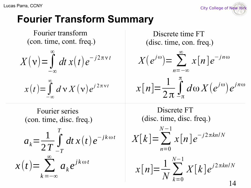
Fourier Transform SummaryFourier transform

(con. time, cont. freq.)Discrete time FT

(disc. time, con. freq.)

Fourier series (con. time, disc. freq.)

Discrete FT (disc. time, disc. freq.)

X ()=∫−∞

∞

dt x( t)e− j 2π t

x (t )=∫−∞

∞

d X ()e j 2π t

X [k ]=∑n=0

N −1

x [n ]e− j 2πkn / N

x [n]=1N

∑k=0

N−1

X [k ]e j 2πkn / N

X (e j ω)= ∑

n=−∞

∞

x [n ]e− j nω

x [n]=1

2π∫−π

π

dω X (e j ω)e j nω

ak=12T

∫−T

T

dt x (t)e− j kω t

x (t)= ∑k=−∞

∞

akej kω t

15


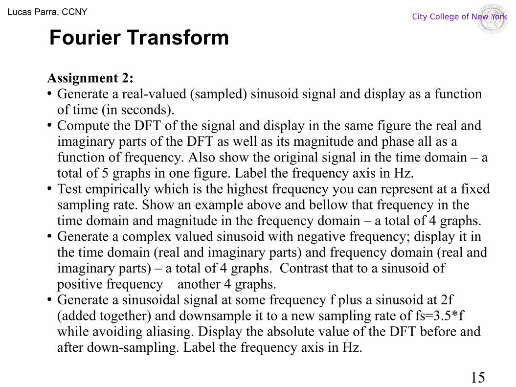
Assignment 2:● Generate a real-valued (sampled) sinusoid signal and display as a function

of time (in seconds).● Compute the DFT of the signal and display in the same figure the real and

imaginary parts of the DFT as well as its magnitude and phase all as a function of frequency. Also show the original signal in the time domain – a total of 5 graphs in one figure. Label the frequency axis in Hz.

● Test empirically which is the highest frequency you can represent at a fixed sampling rate. Show an example above and bellow that frequency in the time domain and magnitude in the frequency domain – a total of 4 graphs.

● Generate a complex valued sinusoid with negative frequency; display it in the time domain (real and imaginary parts) and frequency domain (real and imaginary parts) – a total of 4 graphs. Contrast that to a sinusoid of positive frequency – another 4 graphs.

● Generate a sinusoidal signal at some frequency f plus a sinusoid at 2f (added together) and downsample it to a new sampling rate of fs=3.5*f while avoiding aliasing. Display the absolute value of the DFT before and after down-sampling. Label the frequency axis in Hz.

Fourier Transform

16


What is the relation between a continuous time signal x(t) and its sampled version x[n]?To answer that, compare the continuous time Fourier transform (CTFT) of a continuous time signal x(t) given by,

and the DTFT, X(ejω) of the signal sampled at frequency fs=1/T, x[n]

= x(nT)?

Sampling - Sampling Theorem*

X c =∫−∞

∞

dt x t e− j t

x t =1

2∫−∞

∞

d X c e j t

X e j = ∑

n=−∞

∞

x [n]e− j n

17


According to the Sampling Theorem the relation is:

The DTFT repeats the CTFT with a period 2π.

Contributions above π will overlap with different period!

Sampling - Sampling Theorem

X e j =

1T

∑k=−∞

∞

X c

T

2 kT

ππ ω

Xejω

π/Tπ/T

Xc

Sampling frequency

Nyquist frequency

18


Under which conditions can we determine continuous time x(t) from discrete time x[n], t=nT?

If the signal is bandlimited:

Then we can determine Xc() from X(ejω) according to the

Sampling Theorem:

In that case we can determine x[t] X(ejω) Xc() x(t).

After some algebra:

x(t) is x[n] convolved with

Sampling - Sampling Theorem

x t = ∑n=−∞

∞

x [n ]sinc t−nTT

X e j =

1T

X c

T

X c/T =0, ∣∣≥

sinct =sin t / t

19


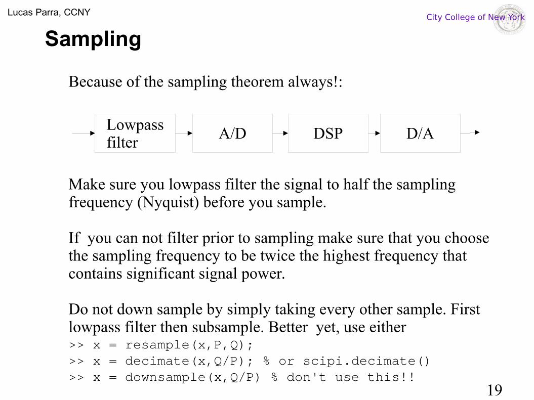
Because of the sampling theorem always!:

Make sure you lowpass filter the signal to half the sampling frequency (Nyquist) before you sample.

If you can not filter prior to sampling make sure that you choose the sampling frequency to be twice the highest frequency that contains significant signal power.

Do not down sample by simply taking every other sample. First lowpass filter then subsample. Better yet, use either>> x = resample(x,P,Q);>> x = decimate(x,Q/P); % or scipi.decimate() >> x = downsample(x,Q/P) % don't use this!!

Sampling

Lowpassfilter

A/D DSP D/A

20


Example: Low-frequency sinusoid (10 Hz) plus noise that is only high-frequency (only components above 25Hz). When sampled at 50Hz without previously removing the high frequency components the HF noise appears at lower frequencies below 25Hz, i.e. it is “reflected” or “leaks” from the high to the low frequencies.

Sampling – what can go wrong

If one fails to low-pass filter before sampling, then frequencies above Nyquist “leak” into the sampled frequency band.

Nyquist

Nyquist

parra lab - bme 50500: image and signal …1 lucas parra, ccny city college of new york bme 50500:...

Documents