part 1- pinch and minimum utility usage · en el delta t min hay transf de calor. composite curve....
TRANSCRIPT

PART 1
PINCH AND MINIMUM UTILITY USAGE

WHAT IS THE PINCH?
• The pinch point is a temperature. • Typically, it divides the temperature range
into two regions. • Heating utility can be used only above the
pinch and cooling utility only below it.

WHAT IS A PINCH DESIGN
• A heat exchanger network obtained using the pinch design method is a network where no heat is transferred from a hot stream whose temperature is above the pinch to a cold stream whose temperature is below the pinch.

IS PINCH TECHNOLGY CURRENT?
• YES and NO. • It is a good first approach to most problems. • Pinch technology is at the root of many other
heat integration technologies. It is impossible to understand them without the basic concepts of pinch technology.
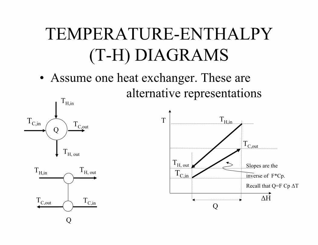
TEMPERATURE-ENTHALPY (T-H) DIAGRAMS
• Assume one heat exchanger. These are alternative representations
TH,in
TC,outTC,in
TH, out
Q
TH, out
TC,out
TH,in
TC,in
Q
Slopes are the
inverse of F*Cp.
Recall that Q=F Cp ∆T
TC,inTC,out
TH,in TH, out
Q
T
∆H

T-H DIAGRAMS
• Assume one heat exchanger and a heater
TH,in
TC,outTC,in
TH, out
TC,inTC,out
TH,in TH, out
Q
Q
TH, out
TC,out
TH,in
TC,in
Q
QH
QH
QHH
T
∆H

T-H DIAGRAMS
• Assume one heat exchanger and a coolerTH,in
TC,outTC,in
TH, out
TC,inTC,out
TH,in TH, out
Q
Q
TH, out
TC,out
TH,in
TC,in
Q
QC
QC
QC
C
T
∆H

T-H DIAGRAMS
• Two hot-one cold streamTH1,in
TC,outTC,in
TH2,out
TC,inTC,out
TH2,in TH2, out
Q1
Q1
TH1,out
TC,out
TH1,in
TC,in
Q1
Q2
Q2
TH2,out
TH2,in
TH1,in TH1,out
Q2
TH2,in
TH2,out
Notice the vertical arrangement of heat transfer
T
∆H

T-H DIAGRAMS• Composite Curve
Remark: By constructing the composite curve we loose information on the vertical arrangement of heat transfer between streams
Obtained by lumping all the heat from different streams that areat the same interval of temperature.
TT
∆H ∆H

T-H DIAGRAMS• Moving composite curves horizontally
TH1,in
TC,out
TC,in
TH1,out
Q1 Q2
TH2,out
TH2,in
Smallest ∆T Smallest ∆T
Cooling
Heating
TH1,in
TC,outTC,in
TH1,out
Q2
TH2,out
TH2,in
QHQ1
QC
TT
∆H ∆H

T-H DIAGRAMS
Moving the cold composite stream to the right
• Increases heating and cooling BY THE SAME AMOUNT
• Increases the smallest ∆T • Decreases the area needed
A=Q/(U* ∆T )
Cooling
Heating
TH1,in
TC,outTC,in
TH1,out
Q2
TH2,out
TH2,in
QHQ1
QC
Smallest ∆T
Notice that for this simple example the smallest ∆T takes place in the end of the cold stream
T
∆H
T-H DIAGRAMS
CoolingHeating
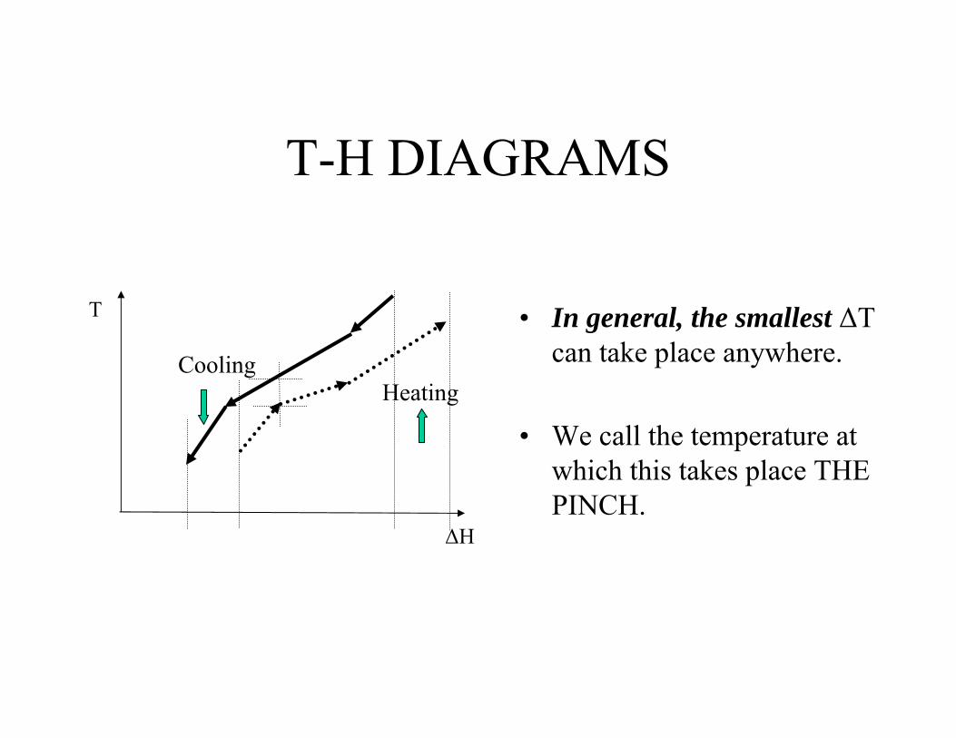
• In general, the smallest ∆T can take place anywhere.
• We call the temperature at which this takes place THE PINCH.
T
∆H

TEMPERATURE-ENTHALPY DIAGRAMS
Cooling
Heating
• From the energy point of view it is then convenient to move the cold stream to the left.
• However, the area may become too large.
• To limit the area, we introduce a minimum approach ∆Tmin
T
∆H
GRAPHICAL PROCEDURE• Fix ∆Tmin
• Construct the hot and cold composite curve• Draw the hot composite curve and leave it fixed• Draw the cold composite curve in such a way that
the smallest ∆T=∆Tmin
• The temperature at which ∆T=∆Tmin is the PINCH• The non-overlap on the right is the Minimum
Heating Utility and the non-overlap on the left is the Minimum Cooling Utility
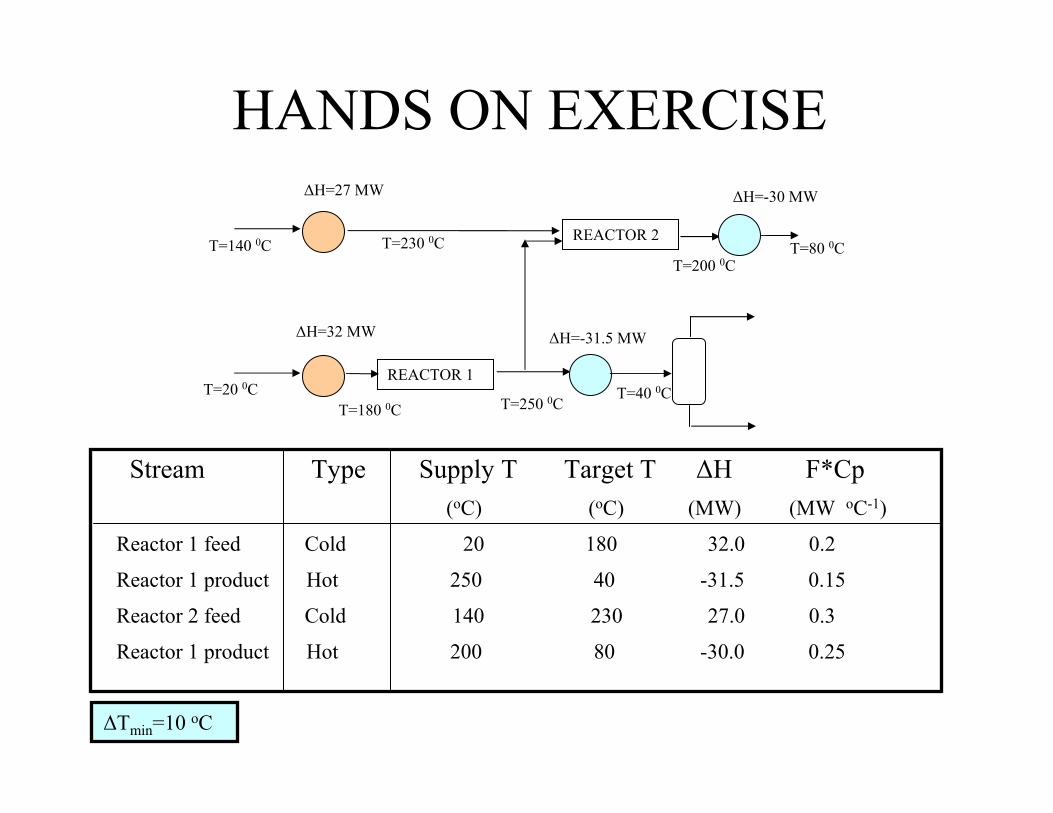
HANDS ON EXERCISE
Stream Type Supply T Target T ∆H F*Cp (oC) (oC) (MW) (MW oC-1)
Reactor 1 feed Cold 20 180 32.0 0.2
Reactor 1 product Hot 250 40 -31.5 0.15
Reactor 2 feed Cold 140 230 27.0 0.3
Reactor 1 product Hot 200 80 -30.0 0.25
T=140 0C
T=20 0C
∆H=27 MW
REACTOR 2
∆H=-30 MW
∆H=32 MW
REACTOR 1
∆H=-31.5 MW
T=230 0C
T=180 0C T=250 0CT=40 0C
T=200 0C
∆Tmin=10 oC
T=80 0C

Answer: Hot Streams
6 48 7.5
250
200
8040 FCp=0.15
FCp=0.4 FCp=0.15
250
200
8040
FCp=
0.15
FCp=
0.25
31.5 30 ∆H ∆H

Answer: Cold Streams FC
p=0.2
FCp=0.3230
180140
20
32 27
FCp=
0.2
FCp=0.3230
180140
20
24 15
FCp=0.5
20∆H ∆H

Answer: Both Curves Together.
Important observation: The pinch is at the beginning of a cold stream or at the beginning of a hot stream.
230
180
140
20
7.5
250
200
80
40
10 51.5
∆T= ∆TminPinch
∆H

UTILITY COST vs. ∆Tmin• There is total overlap for some values of ∆Tmin
Utility
∆Tmin
COST
TOTAL OVERLAP
PARTIAL OVERLAP
Note: There is a particular overlap that requires only cooling utility
T
T
∆H
∆H

PROBLEM TABLE • Composite curves are inconvenient. Thus
a method based on tables was developed.
• STEPS:1. Divide the temperature range into intervals and
shift the cold temperature scale 2. Make a heat balance in each interval3. Cascade the heat surplus/deficit through the
intervals. 4. Add heat so that no deficit is cascaded

PROBLEM TABLE
• We now explain each step in detail. Consider the example 1.1
Stream Type Supply T Target T ∆H F*Cp (oC) (oC) (MW) (MW oC-1)
Reactor 1 feed Cold 20 180 32.0 0.2
Reactor 1 product Hot 250 40 -31.5 0.15
Reactor 2 feed Cold 140 230 27.0 0.3
Reactor 2 product Hot 200 80 -30.0 0.25
∆Tmin=10 oC

PROBLEM TABLE 1. Divide the temperature range into intervals and shift the
cold temperature scale
250
40
200
20
180
140
Hot streams
Cold streams
230
250
40
200190
Hot streams
Cold streams
Now one can make heat balances in each interval. Heat transfer within each interval is feasible.
150
240
30
80 80

PROBLEM TABLE 2. Make a heat balance in each interval. (We now turn into
a table format distorting the scale)
250
80
200
30
150
Hot streams
Cold streams
240
∆Tinterval ∆Hinterval Surplus/Deficit?
10 1.5 Surplus
40 - 6.0 Deficit
10 1.0 Surplus
40 -4.0 Deficit
70 14.0 Surplus
40 -2.0 Deficit
10 - 2.0 Deficit
F Cp=0.15
F Cp=0.25
F Cp=0.2
F Cp=0.3
40
190

PROBLEM TABLE 3. Cascade the heat surplus through the intervals. That is,
we transfer to the intervals below every surplus/deficit. 1.5
- 6.0
1.0
-4.0
14.0
- 2.0
-2.0
This interval has a surplus. It should transfer 1.5 to interval 2.
1.5
1.5
- 6.0
-4.5
1.0
-3.5
-4.0
-7.5
14.0
6.5
-2.0
4.5
- 2.0
2.5
This interval has a deficit. After using the 1.5 cascaded it transfers –4.5 to interval 3.
The largest deficit transferred is -7.5.
Thus, 7.5 MW of heat need to be added on top to prevent any deficit to be transferred to lower intervals
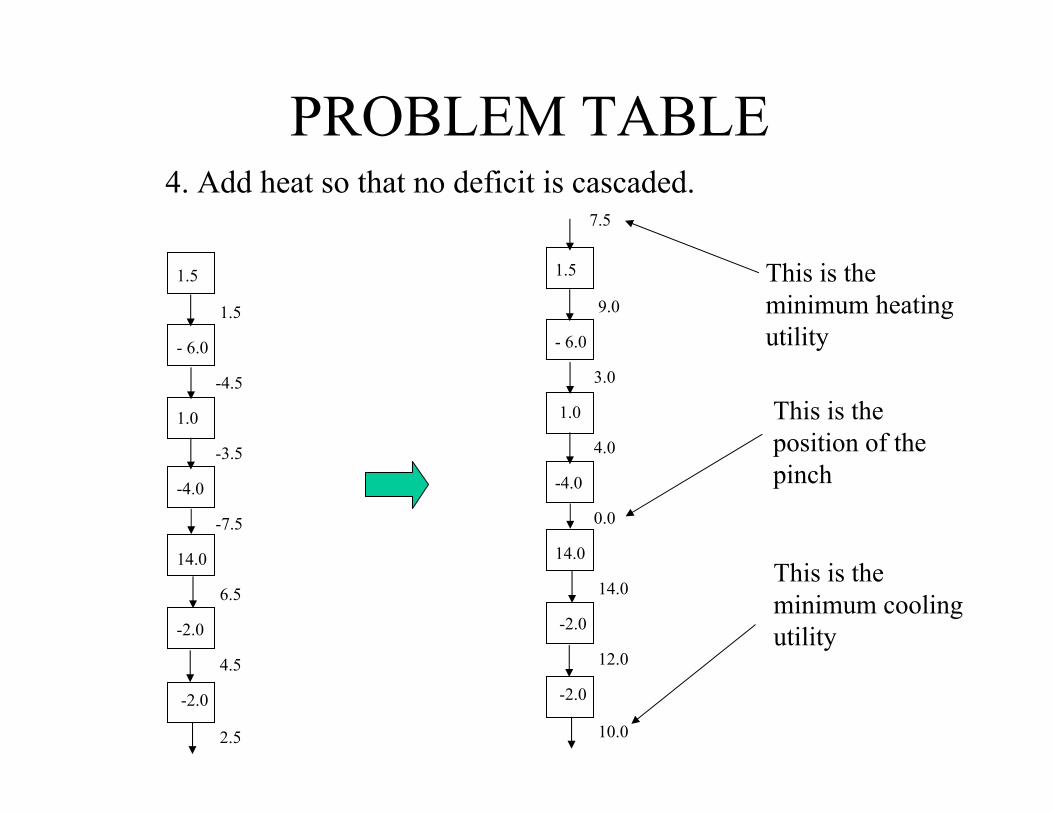
PROBLEM TABLE 4. Add heat so that no deficit is cascaded.
This is the position of the pinch
7.5
1.5
9.0
- 6.0
3.0
1.0
4.0
-4.0
0.0
14.0
14.0
-2.0
12.0
-2.0
10.0
This is the minimum heating utility
This is the minimum cooling utility
1.5
1.5
- 6.0
-4.5
1.0
-3.5
-4.0
-7.5
14.0
6.5
-2.0
4.5
-2.0
2.5
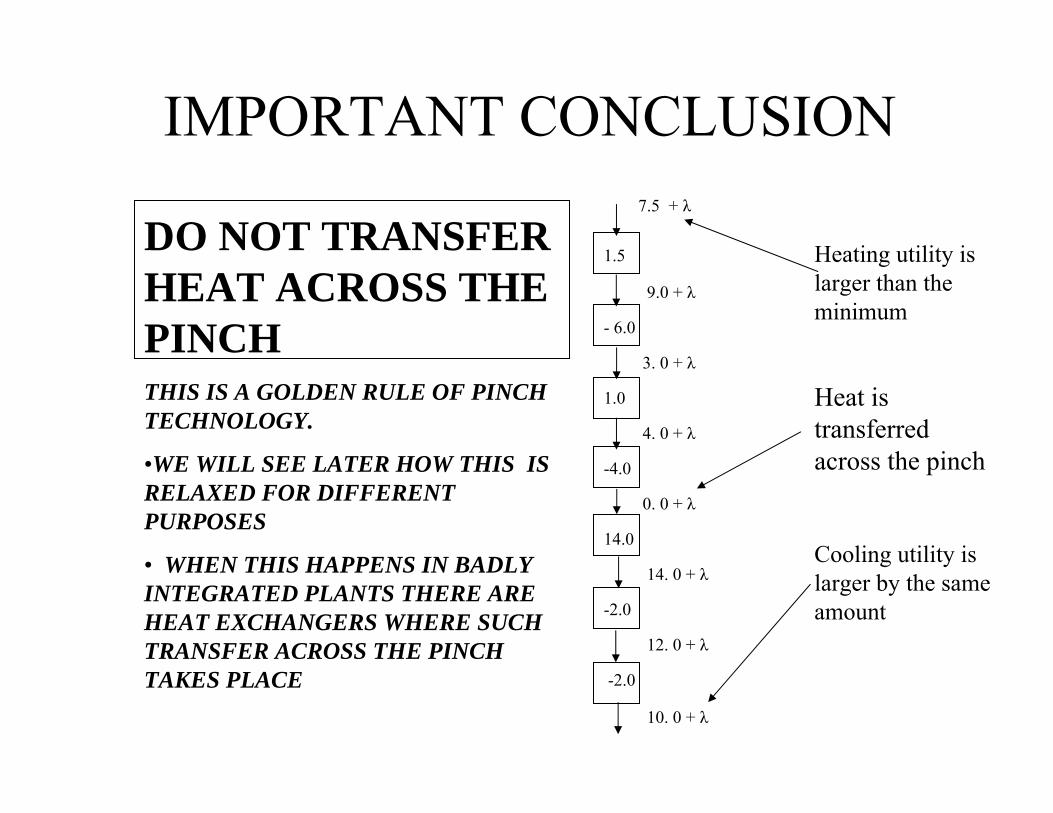
IMPORTANT CONCLUSION
Heat is transferred across the pinch
Heating utility is larger than the minimum
Cooling utility is larger by the same amount
7.5 + λ
1.5
9.0 + λ
- 6.0
3. 0 + λ
1.0
4. 0 + λ
-4.0
0. 0 + λ
14.0
14. 0 + λ
-2.0
12. 0 + λ
-2.0
10. 0 + λ
DO NOT TRANSFER HEAT ACROSS THE PINCHTHIS IS A GOLDEN RULE OF PINCH TECHNOLOGY.
•WE WILL SEE LATER HOW THIS IS RELAXED FOR DIFFERENT PURPOSES
• WHEN THIS HAPPENS IN BADLY INTEGRATED PLANTS THERE ARE HEAT EXCHANGERS WHERE SUCH TRANSFER ACROSS THE PINCH TAKES PLACE

PROBLEM TABLE
These are the minimum values of heating utility needed at each temperature level.
7.5
1.5
9.0
- 6.0
3.0
1.0
4.0
-4.0
0.0
14.0
14.0
-2.0
12.0
-2.0
10.0
Heating utility at the largest temperature is now zero.
0.0
1.5
1.5 + 4.5
- 6.0
0.0
1.0
1.0 + 3.0
-4.0
0.0
14.0
14.0
-2.0
12.0
-2.0
10.0
Heating utility of smaller temperature.

MATHEMATICAL MODELLet be the surplus or demand of heat in interval i . It is given by:
The minimum heating utility is obtained by solving the following linear programming (LP) problem
qi
q F cp T T F cp T Ti kH
kH
i ik
sC
sC
i isi
HiC
= − − −−∈
−∈
∑ ∑( ) ( )1 1Γ Γ
δ0
q1
δ1q2
qi
δiqi+1
δi+1
qn
δn
S Min
s tq i mi i i I
i
min
., ...
=
= + ∀ =≥
−
δ
δ δδ
0
1 10

PART 2
TOTAL AREA TARGETING

TOTAL AREA TARGETINGIn this part we will explore ways to predict the total area of a network without the need to explore specific designs.
Because A=Q/(U*∆Tml), one can calculate the area easily in the following situation.
T
Q
∆Tml=
TH1
TH2
TC1
TC2
(TH1-TC2)-(TH2-TC1)(TH1-TC2)(TH2-TC1)
ln
∆H

TOTAL AREA TARGETINGSince area=Q/(U ∆Tml), the composite curve diagram provides one way of estimating the total area involved. Isolate all regions with a pair of straight line sections and calculate the area for each.
Cooling water
Heating utility, steam or furnace.
A1 A4 A5 A6A3A2
The above scheme of heat transfer is called VERTICAL HEAT TRANSFER
∆H
T

EXERCISECalculate the values of Q in each interval and estimate the corresponding area. Use U= 0.001 MW m-2 oC
Furnace (300 oC)
Obtain the total
area estimateCooling Water
230
180
140
20
250
200
80
40
∆T= ∆TminPinch
Q1Q2 Q6Q3 Q4 Q5
∆H
T

COMPOSITE CURVE
0
50
100
150
200
250
300
0 10 20 30 40 50 60 70 80 90
Q, MW
T, C
HOT COLD
I II III IV
V VI
EXERCISE
Interval Q TH1 TH2 TC1 TC2
Units:
Q= MW
T= oC
A= m2
Furnace (300 oC)
Cooling Water
∆T= ∆Tmin
Pinch
I 6 80 40 15 20II 4 90 80 20 30III 24 150 90 20 140IV 20 200 150 140 180V 7.5 250 200 180 205VI 7.5 300 250 205 230

EXERCISE
Interval Q TH1 TH2 TC1 TC2 ∆Tml A
Units: Q= MW T= oC , A= m2
U= 0.001 MW m-2 oC
I 6 80 40 15 20 40.0 150.1II 4 90 80 20 30 60.0 66.7III 24 150 90 20 140 30.8 778.4IV 20 200 150 140 180 14.4 1386.3V 7.5 250 200 180 205 30.8 243.3VI 7.5 300 250 205 230 81.9 91.6
Total Area 2716.3
TOTAL AREA TARGETINGDrawbacks
• Fixed costs associated with the number of units are not considered.
We will see later how the number of units can be calculated

QUESTIONS FOR DISCUSSION
• Is the total area predicted this way, realistic? That is, is it close enough to a value that one would obtain in a final design?
• Is the estimate, realistic or not, conservative? That is, is it larger than the one expected from a final design?
•How complex is a design built using the vertical transfer?

ANSWERS
• Is the total area predicted this way, realistic? That is, is it close enough to a value that one would obtain from a final design?
YES, Within 10-15%

ANSWERS
•Is the estimate, realistic or not, conservative? That is, is it larger than the one expected from a final design?
The area obtained is actually the minimum area needed to perform the heat transfer.

ANSWERS•How complex is a design built using the vertical transfer?
Very Complex. Take for example interval 4. There are four streams in this interval.
Stream Type Supply T Target T ∆H F*Cp
(oC) (oC) (MW) (MW oC-1)
Reactor 1 feed Cold 140 180 8.0 0.2
Reactor 1 product Hot 200 150 -7.5 0.15
Reactor 2 feed Cold 140 180 12.0 0.3
Reactor 1 product Hot 200 150 -12.5 0.25
This implies at least three heat exchangers, just in this interval.

HEAT EXCHANGER NETWORK
R1 prod, FCp=0.15
R2 prod, FCp=0.25
R1 feed, FCp=0.2
R2 feed, FCp=0.3
VI
FCp=0.1875
FCp=0.1125
FCp=0.09FCp=0.16
80 90 150 200 250 30040
20 30 140 180 205 2301520
VIVIIIIII
300

HEAT EXCHANGER NETWORK
R1 prod, FCp=0.15
R2 prod, FCp=0.25
R1 feed, FCp=0.2
R2 feed, FCp=0.3
VIFCp=0.1125
FCp=0.16
80 90 150 200 250 30040
20
20
140 180 205 23015 30
VIVIIIIII
300
FCp=0.075
TOTAL= 10 ExchangersCalled “Spaghetti” design

PREDICTING THE NUMBER OF UNITS
We can anticipate very simply how many exchangers we should have!!!
Consider the following warehouses, each containing some merchandise that needs to be delivered to the row of consumer centers. What is the minimum number of trucks needed?
561625
175030Warehouses
Consumer Centers
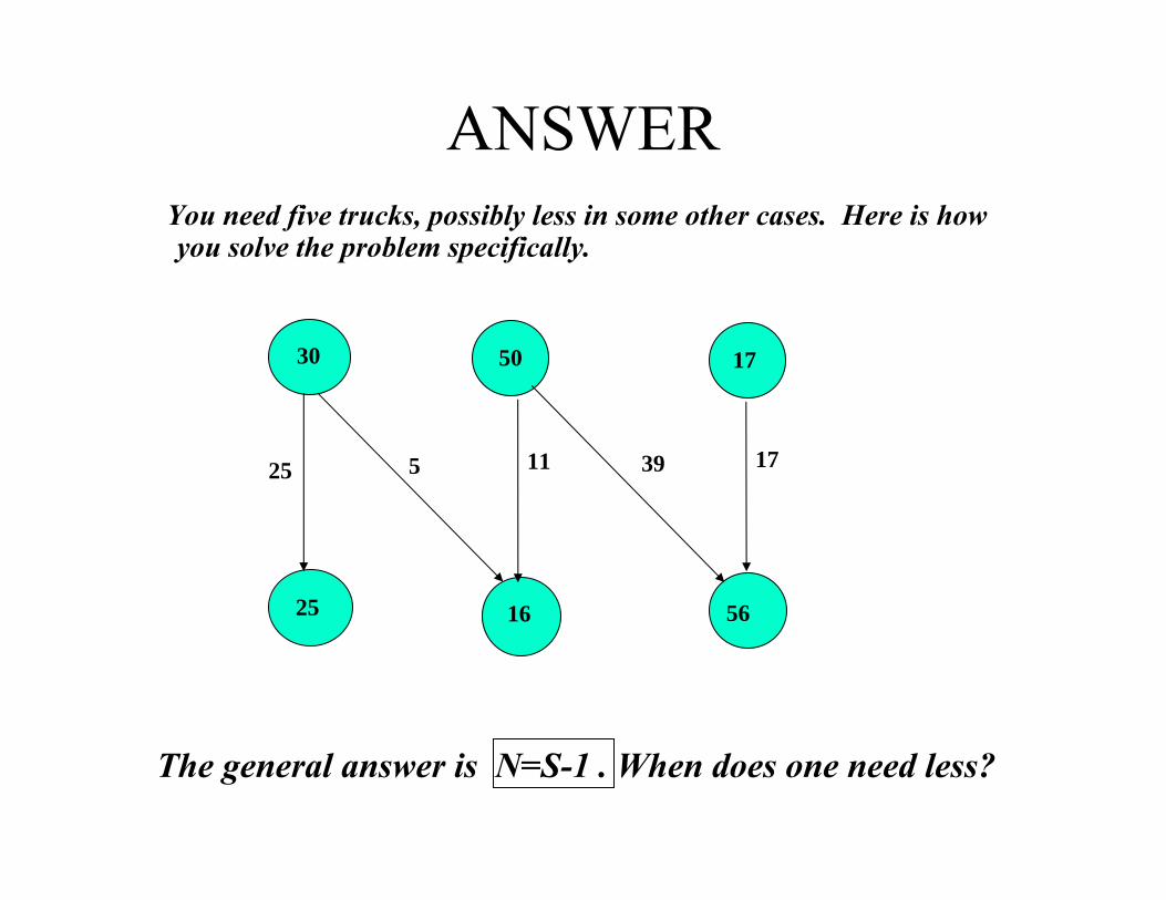
ANSWERYou need five trucks, possibly less in some other cases. Here is how you solve the problem specifically.
561625
175030
25 5 11 39 17
The general answer is N=S-1 . When does one need less?

ANSWERWhen there is an exact balance between two streams or a subset of streams.
561625
175525
25 16 39 17
The general answer is N=S-P . P is the number of independent subsystems. (Two in this case)

GENERAL FORMULA FOR UNIT TARGETING
Nmin= (S-P)above pinch+ (S-P)below pinch
If we do not consider two separate problems, above and below the pinch we can get misleading results.
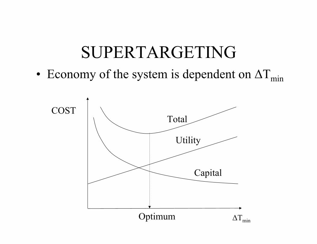
SUPERTARGETING• Economy of the system is dependent on ∆Tmin
Utility
Capital
Total
∆Tmin
COST
Optimum

SPECIAL CASES• There is total overlap for some values of ∆Tmin
Utility
Capital
Total
∆Tmin
COST
TOTAL OVERLAP
PARTIAL OVERLAP
Note: There is a particular overlap that requires only cooling utility
T
T
∆H
∆H

PART 3
DESIGN OF MAXIMUM ENERGY RECOVERY
NETWORKS

MER NETWORKS
• Networks featuring minimum utility usage are called MAXIMUM ENERGY RECOVERY (MER) Networks.

PINCH DESIGN METHOD
RECALL THAT• No heat is transferred through the pinch. • This makes the region above the pinch a
HEAT SINK region and the region below the pinch a HEAT SOURCE region.

Pinch
Minimum heating utility
Minimum cooling utilityHeat Source
Heat is released to cooling utility
Heat SinkHeat is obtained from the heating utility
7.5
12.0
14.0
0.0
-6.0
1.0
-4.0
4.0
3.0
9.0
-2.0
-2.0
14.0
1.5
10.0
T
H
CONCLUSION
• One can analyze the two systems separately, that is,
• Heat exchangers will not contain heat transfer across the pinch.

PINCH MATCHES• Consider two streams above the pinch
Q/FCpH > Q/FCpC
Tp- ∆TminTC,outQ
TH,inTp
TC,out= Tp- ∆Tmin + Q/FCpC
TH,in= Tp+Q/FCpH
But TH,in> TC,out+ ∆Tmin.
Thus replacing one obtains
FCpH < FCpC Golden rule for pinch matches above the pinch.
∆Tmin Violation when FCpH > FCpC∆Tmin

TH,out
Tp- ∆Tmin
TC,inQ
Tp
TC,in= Tp- ∆Tmin - Q/FCpC
TH,out= Tp-Q/FCpH
But TH,out> TC,in + ∆Tmin.
Thus replacing one obtains
FCpC < FCpH Golden rule for pinch matches below the pinch.
∆Tmin∆Tmin
Violation when FCpC > FCpH
•Consider two streams below the pinch
PINCH MATCHES

CONCLUSION
• Since matches at the pinch need to satisfy these rules, one should start locating these matches first. Thus, our first design rule:
START BY MAKING PINCH MATCHES

QUESTION
• Once a match has been selected how much heat should be exchanged?

ANSWER
• As much as possible!• This means that one of the streams has its duty
satisfied!!
THIS IS CALLLED THE
TICK-OFF RULE

HANDS ON EXERCISE
Stream Type Supply T Target T ∆H F*Cp (oC) (oC) (MW) (MW oC-1)
Reactor 1 feed Cold 20 180 32.0 0.2
Reactor 1 product Hot 250 40 -31.5 0.15
Reactor 2 feed Cold 140 230 27.0 0.3
Reactor 1 product Hot 200 80 -30.0 0.25
T=140 0C
T=20 0C
∆H=27 MW
REACTOR 2
∆H=-30 MW
∆H=32 MW
REACTOR 1
∆H=-31.5 MW
T=230 0C
T=180 0C T=250 0C T=40 0C
T=200 0CT=80 0C
∆Tmin=10 oC PINCH=150 oC

HANDS ON EXERCISE
Stream Type Supply T Target T ∆H F*Cp (oC) (oC) (MW) (MW oC-1)
Reactor 1 feed Cold 20 180 32.0 0.2
Reactor 1 product Hot 250 40 -31.5 0.15
Reactor 2 feed Cold 140 230 27.0 0.3
Reactor 1 product Hot 200 80 -30.0 0.25
∆Tmin=10 oC PINCH=150 oC
200 0C
20 0C
40 0C
180 0C
250 0CH1
H2
C2
C1
230 0C
FCp=0.15
FCp=0.25
FCp=0.2
FCp=0.3
140 0C
80 0C
150 0C

ABOVE THE PINCH
• Which matches are possible?
200 0C
180 0C
250 0CH1
H2
C2
C1
230 0C
FCp=0.15
FCp=0.25
FCp=0.2
FCp=0.3140 0C
150 0C

ANSWER (above the pinch)
200 0C
180 0C
250 0CH1
H2
C2
C1
230 0C
FCp=0.15
FCp=0.25
FCp=0.2
FCp=0.3140 0C
150 0C
• The rule is that FCpH < FCpC . We therefore can only make the match H1-C1 and H2-C2.

ANSWER (above the pinch)
• The tick-off rule says that a maximum of 8 MW is exchanged in the match H1-C1 and as a result stream C1 reaches its target temperature.
• Similarly 12.5 MW are exchanged in the other match and the stream H2 reaches the pinch temperature.
200 0C
180 0C
203.3 0CH1
H2
C2
C1 181.7 0C
FCp=0.15
FCp=0.25
FCp=0.2
FCp=0.3140 0C
150 0C
8
12.5
230 0C
250 0C

BELOW THE PINCH
• Which matches are possible?
20 0C
40 0CH1
H2
C1
FCp=0.15
FCp=0.25
FCp=0.2 140 0C
80 0C
150 0C
The rule is that FCpC < FCpH . Thus, we can only make the match H2-C1

ANSWER (below the pinch)
• The tick-off rule says that a maximum of 17.5 MW is exchanged in the match H2-C1 and as a result stream H2 reaches its target temperature.
52.5 0C
40 0CH1
H2
C1
FCp=0.15
FCp=0.25
FCp=0.2 140 0C
80 0C
150 0C
17.5
20 0C

COMPLETE NETWORK AFTER PINCH MATCHES
• Streams with unfulfilled targets are colored.
200 0C
180 0C
203.3 0CH1
H2
C2
181.7 0C
FCp=0.15
FCp=0.25
FCp=0.2
FCp=0.3140 0C
8
12.5
52.5 0C C1
140 0C
80 0C
150 0C
17.5
250 0C
230 0C
20 0C
40 0C

WHAT TO DO NEXT?
• Away from the pinch, there is more flexibility to make matches, so the inequalities do not have to hold.
• The pinch design method leaves you now on your own!!!!!• Therefore, use your judgment as of what matches to select!!
200 0C
180 0C
203.3 0CH1
H2
C2
181.7 0C
FCp=0.15
FCp=0.25
FCp=0.2
FCp=0.3140 0C
8
12.5
52.5 0C C1
140 0C
80 0C
150 0C
17.5
250 0C
230 0C
20 0C
40 0C

ANSWER
• We first note that we will use heating above the pinch. Thus all hot streams need to reach their inlet temperature. We are then forced to look for a match for H1. Please locate it.
200 0C
180 0C
203.3 0CH1
H2
C2
181.7 0C
FCp=0.15
FCp=0.25
FCp=0.2
FCp=0.3140 0C
8
12.5
52.5 0C C1
140 0C
80 0C
150 0C
17.5
250 0C
230 0C
20 0C
40 0C

ANSWER
140 0C
• The match is H1-C1. We finally put a heater on the cold stream
200 0C
180 0C
H1
H2
C2
230 0C
FCp=0.15
FCp=0.25
FCp=0.2
FCp=0.38
12.5
52.5 0C C1
140 0C
80 0C
150 0C
17.5
77.5
H
250 0C
20 0C
40 0C

ANSWER • Below the pinch we try to have the cold streams start at
their inlet temperatures and we later locate coolers (one in this case).
140 0C
200 0C
180 0C
H1
H2
C2 230 0C
FCp=0.15
FCp=0.25
FCp=0.2
FCp=0.38
12.5
20 0C C1 140 0C
80 0C
150 0C
17.5
77.5
H6.5
C
10
40 0C250 0C

EXAMPLE
Nmin= (S-P)above pinch+ (S-P)below pinch ==(5-1) + (4-1) = 7
If we do not consider two separate problems Nmin= (6-1)= 5, which is wrong
Note: A heat exchanger network with 5 exchangers exists, but it is impractical and costly. This is beyond the scope of this course.
140 0C
200 0C
180 0C
H1
H2
C2
230 0C
FCp=0.15
FCp=0.25
FCp=0.2
FCp=0.38
12.5
20 0C C1 140 0C
80 0C
150 0C
17.5
77.5
H6.5
C
10
250 0C 40 0C
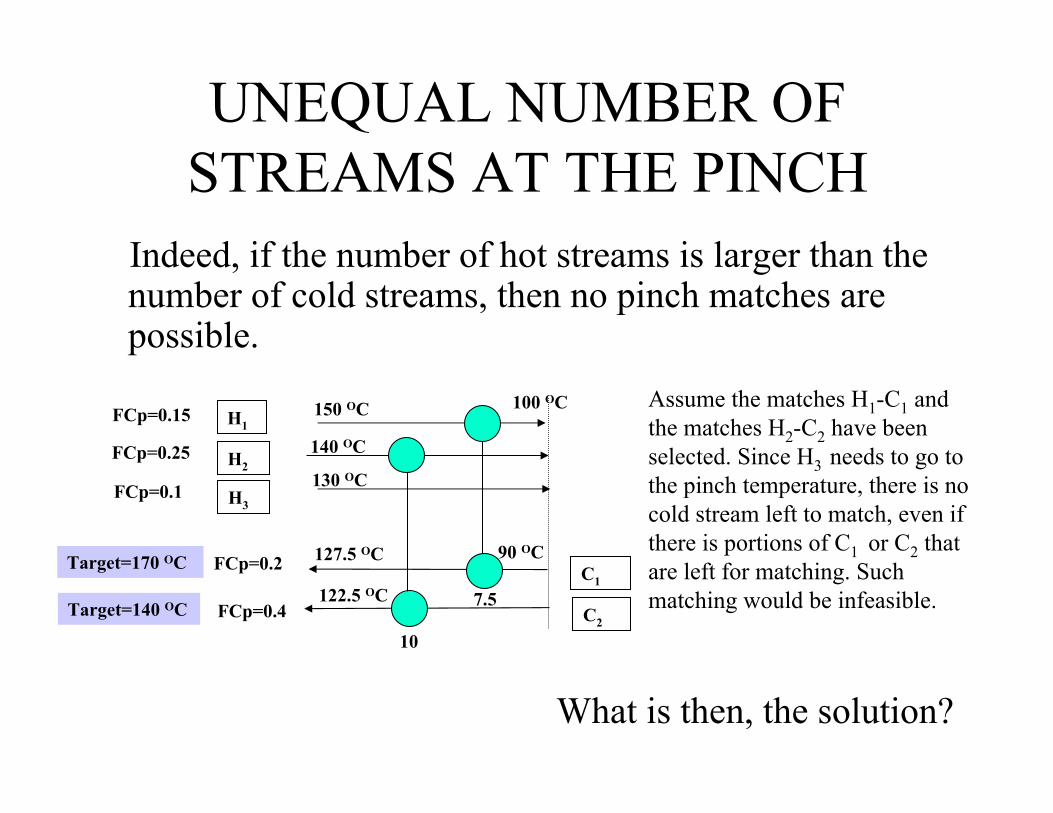
UNEQUAL NUMBER OF STREAMS AT THE PINCH
Indeed, if the number of hot streams is larger than the number of cold streams, then no pinch matches are possible.
C2
C1
H1
H2
H3
Assume the matches H1-C1 and the matches H2-C2 have been selected. Since H3 needs to go to the pinch temperature, there is no cold stream left to match, even if there is portions of C1 or C2 that are left for matching. Such matching would be infeasible.
150 OC 100 OCFCp=0.15
FCp=0.25
FCp=0.2
FCp=0.4
FCp=0.1
90 OC
7.5
140 OC
10
Target=170 OC 127.5 OC
122.5 OCTarget=140 OC
130 OC
What is then, the solution?
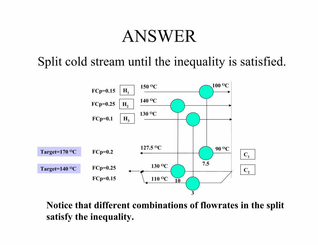
ANSWER Split cold stream until the inequality is satisfied.
Notice that different combinations of flowrates in the split satisfy the inequality.
C2
C1
H1
H2
H3
150 OC 100 OCFCp=0.15
FCp=0.25
FCp=0.2
FCp=0.25
FCp=0.1
90 OC
7.5
140 OC
10
Target=170 OC127.5 OC
130 OCTarget=140 OC
130 OC
FCp=0.15 110 OC
3

INEQUALITY NOT SATISFIED
Consider the following case:
C2
C1
H1 150 OC 100 OC
FCp=0.5
FCp=0.2
FCp=0.4
90 OCTarget=170 OC
Target=140 OC

ANSWER Split the hot stream
C2
C1
H1 150 OC 100 OCFCp=0.2
FCp=0.2
FCp=0.4
90 OC
15
Target=170 OC
Target=140 OC
FCp=0.3
10
140 OC
127.5 OC

SOLVE THE FOLLOWING PROBLEM
Below the Pinch :
C1
H2
H1 100 OC
FCp=0.5
FCp=0.3
FCp=0.7 90 OC
Target=40 OC
Target=20 OC
30 OC

ANSWER Below the Pinch :
30C1
H2
H1 100 OC
FCp=0.5
FCp=0.3
FCp=0.590 OC
Target=40 OC
Target=20 OC
30 OC
FCp=0.2
12
40 OC
60 OC

COMPLETE PROCEDUREABOVE THE PINCH
Start
SH≤SC
Split Cold Stream
FCpH≤FCpC
at pinch?
Place matches
Split Hot Stream
YesYes
NoNo

COMPLETE PROCEDUREBELOW THE PINCH
SH≥SC
Split Hot Stream
FCpH ≥ FCpCat pinch?
Split Cold Stream
Start
Place matches
YesYes
No No

HANDS ON EXERCISEType Supply T Target T F*Cp
(oC) (oC) (MW oC-1)
Hot 750 350 0.045
Hot 550 250 0.04
Cold 300 900 0.043
Cold 200 550 0.02
∆Tmin=50 oC
Minimum Heating Utility= 9.2 MW
Minimum Cooling Utility= 6.4 MW

ANSWER
750 0C
900 0C
H1
H2
C2
FCp=0.045
FCp=0.04
FCp=0.043
FCp=0.02
500 0C
8
C1
250 0C
61
9.2
300 0C
8.6
0.4
550 0C
550 0C
6
350 0C
200 0C
FCp=0.04
686.05 0C 400 0C
358.89 0C

TRANSSHIPMENT MODEL(Papoulias and Grossmann, 1983)
We will now expand the mathematical model we presented to calculate the minimum utility.
∑∑Γ∈
−Γ∈
− −−−=Ci
Hi s
iiCs
Cs
kii
Hk
Hki TTcpFTTcpFq )()( 11
δ0
q1
δ1q2
qi
δiqi+1
δi+1
q
δn
S Min
s tq i mi i i I
i
min
., ...
=
= + ∀ =≥
−
δ
δ δδ
0
1 10
Where

TRANSSHIPMENT MODELAssume now that we do the same cascade for each hot stream, while we do not cascade the cold streams at all. In addition we consider heat transfer from hot to cold streams in each interval.
The material balances for hot streams are:
The material balances for cold streams are:
Where ri,j and pk,j are the heat content of hot stream I and cold stream k in interval j.
Ijkik
jijiji
i
mjsr ,...1
0
,,,1,,
0,
=∀−+=
=
∑−δδ
δ
Ijkii
jk mjsp ,...1,,, =∀=∑
si,k,1ri,1 pk,1
δi,1 si,k,2
ri,2 pk,2
si,k,jri,j pk,j
δi,j si,k,,j+1
ri,j+1 pk,j+1
δi,j+1
si,k,nri,n pk,n
δi,n

TRANSSHIPMENT MODELAlthough we have a simpler model to solve it, in this new framework, the minimum utility problem becomes:
Note that the set of hot streams now includes process streams and the utility U. Cold streams include cooling water.
Ijkii
jk
Ijkik
jijiji
Ii
U
mjksp
mjisr
mjits
Min
,...1,
,...1,
,...1,0.
,,,
,,,1,,
0,
0,
=∀∀=
=∀∀−+=
=∀∀=
∑
∑−δδ
δ
δ
si,k,1ri,1 pk,1
δi,1 si,k,2
ri,2 pk,2
si,k,jri,j pk,j
δi,j si,k,,j+1
ri,j+1 pk,j+1
δi,j+1
si,k,nri,n pk,n
δi,n

TRANSSHIPMENT MODELWe would like to have a model that would tell us the si,k,j such that the number of units is minimum. We now introduce a way of counting matches between streams. Let Yi,k be a binary variable (can only take the value 0 or 1).
Then we can force Yi,k to be one using the following inequality
indicating therefore that heat has been transferred from stream i to stream k in at least one interval.
0,,, ≤Γ−∑ kijkij
Ys
si,k,1ri,1 pk,1
δi,1 si,k,2
ri,2 pk,2
si,k,jri,j pk,j
δi,j si,k,,j+1
ri,j+1 pk,j+1
δi,j+1
si,k,nri,n pk,n
δi,n
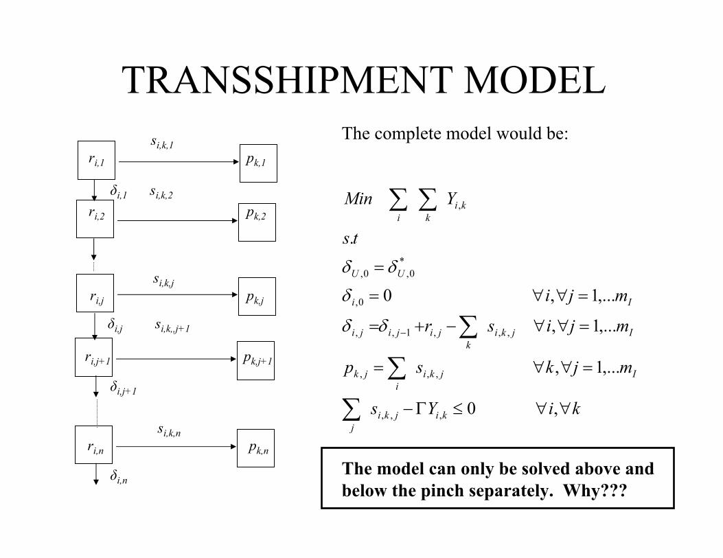
TRANSSHIPMENT MODELThe complete model would be:
The model can only be solved above and below the pinch separately. Why???
kiYs
mjksp
mjisr
mji
ts
YMin
kijkij
Ijkii
jk
Ijkik
jijiji
Ii
UU
kiki
∀∀≤Γ−
=∀∀=
=∀∀−+=
=∀∀=
=
∑
∑
∑
∑∑
−
,0
,...1,
,...1,
,...1,0
.
,,,
,,,
,,,1,,
0,
*0,0,
,
δδ
δδδ
si,k,1ri,1 pk,1
δi,1 si,k,2
ri,2 pk,2
si,k,jri,j pk,j
δi,j si,k,,j+1
ri,j+1 pk,j+1
δi,j+1
si,k,nri,n pk,n
δi,n

TRANSSHIPMENT MODEL
We are minimizing the number of matches. Different answers can be obtained if separate regions are not considered. These answers are not guaranteed to be realistic.
GAMS MODEL
GAMS MODEL
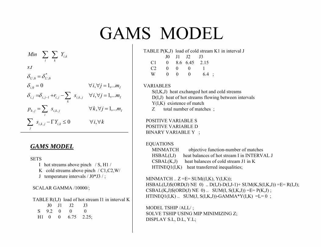
SETSI hot streams above pinch / S, H1 /K cold streams above pinch / C1,C2,W/ J temperature intervals / J0*J3 / ;
SCALAR GAMMA /10000/;
TABLE R(I,J) load of hot stream I1 in interval KJ0 J1 J2 J3
S 9.2 0 0 0H1 0 0 6.75 2.25;
kiYs
mjksp
mjisr
mji
ts
YMin
kijkij
Ijkii
jk
Ijkik
jijiji
Ii
UU
kiki
∀∀≤Γ−
=∀∀=
=∀∀−+=
=∀∀=
=
∑
∑
∑
∑∑
−
,0
,...1,
,...1,
,...1,0
.
,,,
,,,
,,,1,,
0,
*0,0,
,
δδ
δδδ
TABLE P(K,J) load of cold stream K1 in interval J J0 J1 J2 J3
C1 0 8.6 6.45 2.15 C2 0 0 0 1 W 0 0 0 6.4 ;
VARIABLESS(I,K,J) heat exchanged hot and cold streamsD(I,J) heat of hot streams flowing between intervalsY(I,K) existence of match Z total number of matches ;
POSITIVE VARIABLE SPOSITIVE VARIABLE DBINARY VARIABLE Y ;
EQUATIONSMINMATCH objective function-number of matchesHSBAL(I,J) heat balances of hot stream I in INTERVAL JCSBAL(K,J) heat balances of cold stream J1 in KHTINEQ1(I,K) heat transferred inequalities;
MINMATCH .. Z =E= SUM((I,K), Y(I,K));HSBAL(I,J)$(ORD(J) NE 0) .. D(I,J)-D(I,J-1)+ SUM(K,S(I,K,J)) =E= R(I,J);CSBAL(K,J)$(ORD(J) NE 0) .. SUM(I, S(I,K,J)) =E= P(K,J) ;HTINEQ1(I,K) .. SUM(J, S(I,K,J))-GAMMA*Y(I,K) =L= 0 ;
MODEL TSHIP /ALL/ ;SOLVE TSHIP USING MIP MINIMIZING Z;DISPLAY S.L, D.L, Y.L;
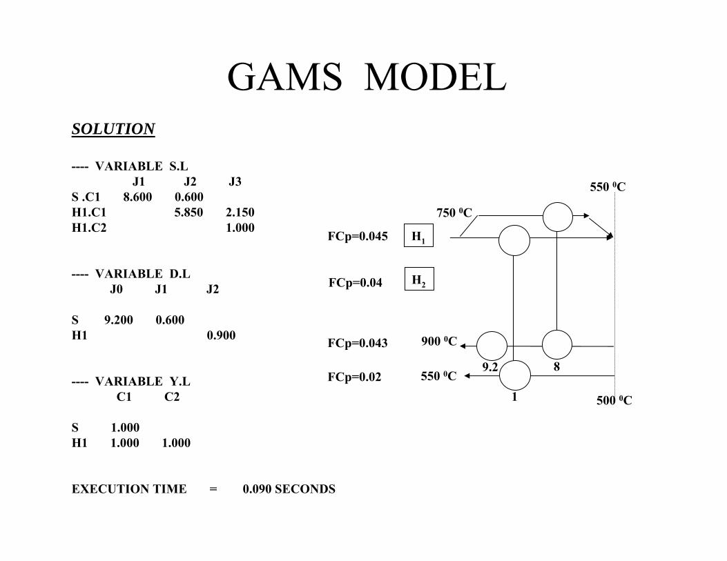
GAMS MODEL SOLUTION
---- VARIABLE S.L J1 J2 J3
S .C1 8.600 0.600H1.C1 5.850 2.150H1.C2 1.000
---- VARIABLE D.LJ0 J1 J2
S 9.200 0.600H1 0.900
---- VARIABLE Y.L C1 C2
S 1.000H1 1.000 1.000
EXECUTION TIME = 0.090 SECONDS
750 0C
900 0C
H1
H2
FCp=0.045
FCp=0.04
FCp=0.043
FCp=0.02
500 0C
8
1
9.2
550 0C
550 0C

PART 4
UTILITY PLACEMENT HEAT AND POWER
INTEGRATION

UTILITY PLACEMENT We now introduce the GRAND COMPOSITE CURVE, which will be useful to analyze the placement of utilities.
1.5
- 6.0
1.0
-4.0
14
-2.0
-2.0
Start at the pinch
Pinch
250
40
200190
150
240
30
80
∆H
T

GRAND COMPOSITE CURVE
These are called “pockets”
Process-to Process integration takes place here
Total heating utility
250
40
200190
150
240
30
80
Total cooling utility
∆H
T

UTILITY PLACEMENT We now resort to a generic grand composite curve to show how utilities are placed.
Cooling Water
∆H
T HP Steam
LP Steam
MP Steam
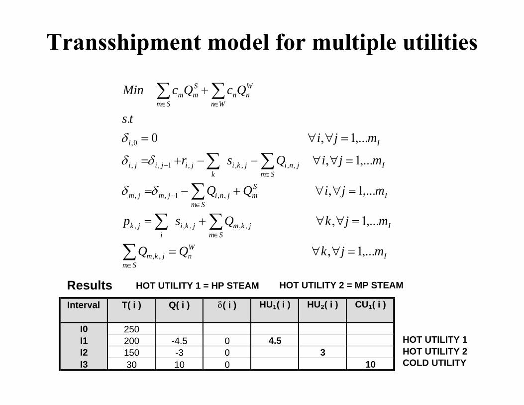
Transshipment model for multiple utilities
IWn
Smjkm
ISm
jkmjkii
jk
ISm
Smjnijmjm
ISm
jnijkik
jijiji
Ii
Wn
Wnn
Sm
Smm
mjkQQ
mjkQsp
mjiQQ
mjiQsr
mjits
QcQcMin
,...1,
,...1,
,...1,
,...1,
,...1, 0.
,,
,,,,,
,,1,,
,,,,,1,,
0,
=∀∀=
=∀∀+=
=∀∀+−=
=∀∀−−+=
=∀∀=
+
∑
∑∑
∑
∑∑
∑∑
∈
∈
∈−
∈−
∈∈
δδ
δδ
δ
Results
HOT UTILITY 1HOT UTILITY 2COLD UTILITY
Interval T( i ) Q( i ) δ( i ) HU1( i ) HU2( i ) CU1( i )
I0 250I1 200 -4.5 0 4.5I2 150 -3 0 3I3 30 10 0 10
HOT UTILITY 1 = HP STEAM HOT UTILITY 2 = MP STEAM

UTILITY PLACEMENT Hot Oil placement and extreme return temperatures
Hot oil from furnace
∆H
Oil minimum return temperature
Water maximum return temperature
Process
T
Cooling water
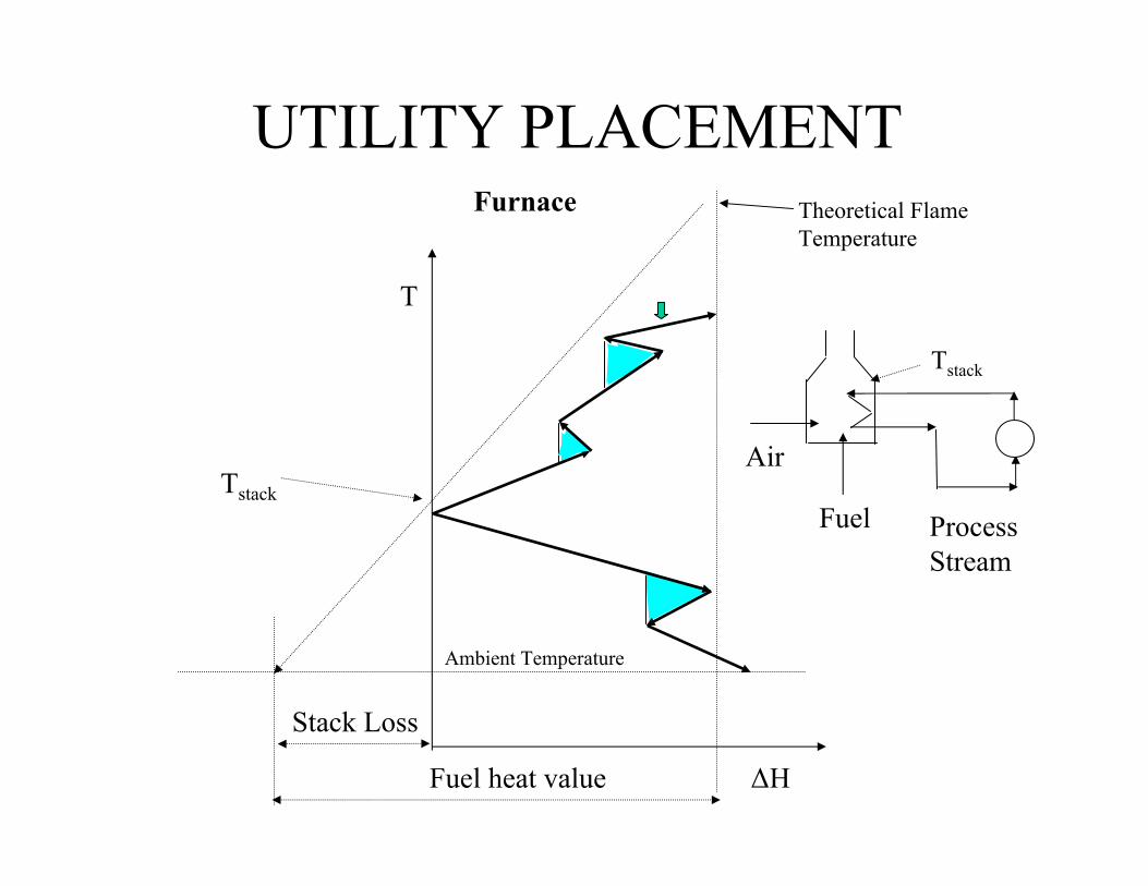
UTILITY PLACEMENT Furnace Theoretical Flame
Temperature
T
∆H
Tstack
Process Stream
Ambient Temperature
Air
Fuel
Fuel heat value
Stack Loss
Tstack

COMBINED HEAT AND POWER
Note that in this case there is no gain. The heat engine can be arranged separately and the utility usage will not change.
T
T
Pinch
QH,min
QHE
QHE -W
QC,min +( QHE –W)
Integration of a Heat Engine below the Pinch.
W

COMBINED HEAT AND POWER
T
Pinch
QH,min -( QHE –W)QHE
QHE -W
QC,min
Integration of a Heat Engine Across the Pinch.
W
TOTAL HEN ENERGY INTAKE
QH,min -( QHE –W)
(Smaller)
SYSTEM TOTAL ENERGY INTAKE
QH,min+W
vs. QH,min+QHE
(separate)

INTEGRATION WITH DISTILLATION
In this case there is a gain of (Qcond - Qreb)in the cooling utility.
QC,min + (Qcond - Qreb)
Placement below the pinch.
T
Pinch
QH,min
Qreb
Qcond
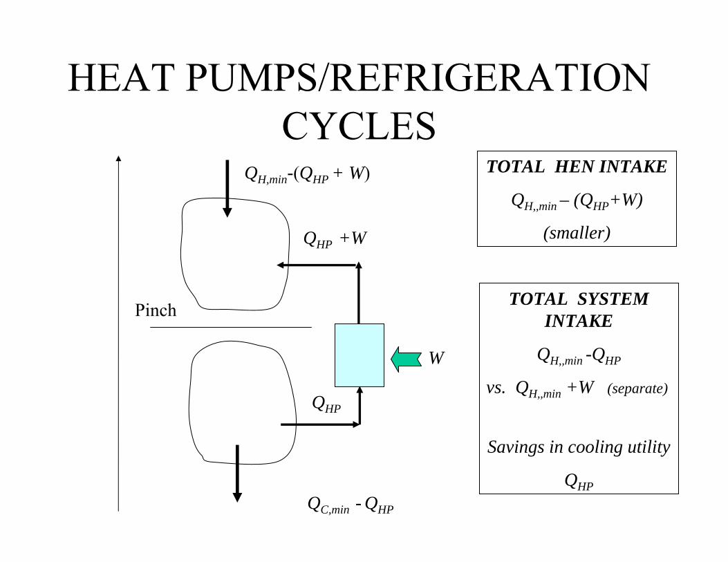
Pinch
QH,min-(QHP + W)
QHP +W
QHP
QC,min - QHP
W
TOTAL HEN INTAKE
QH,,min – (QHP+W)
(smaller)
HEAT PUMPS/REFRIGERATION CYCLES
TOTAL SYSTEM INTAKE
QH,,min -QHP
vs. QH,,min +W (separate)
Savings in cooling utility
QHP

COMBINED HEAT AND POWER
QHE
Utility Placement
T
Pinch QLP
QC,min
W
QH,min –( QHP+QLP)
QHP
QC,min
QHP
QLP
T
∆H
TOTAL HEN INTAKE
QH,min –( QHP+QLP)(smaller)
TOTAL SYSTEM INTAKE
QH,min +W
vs. QH,min+W+(QHP + QLP)(separate)

COMBINED HEAT AND POWER
QF
Gas Turbine Placement
T
PinchQS
QC,min
W
QH,min -QS
QLOSS
Air
T0
TEX
T
∆H
T0
QF -W
QLOSS
TEX
QS
TOTAL ENERGY INTAKE
QH,min + W+ QLOSS
vs. QH,min + W+ QLOSS+QS

PART 5
DISTILLATION PLACEMENT

PLACEMENT OF DISTILLATION
Note that in this case there is no gain. The distillation column can be arranged separately and the utility usage will not change.
T
Pinch
QH,min + Qreb
Qreb
Qcond
QC,min + Qcond
Placement across the pinch.

PLACEMENT OF DISTILLATION
Note that in this case there is a possible gain in the heating utility.
T
Pinch
QH,min + Qreb - Qcond
Qreb
Qcond
QC,min
Placement above the pinch.

ADJUSTING PRESSURE FOR PROPER PLACEMENT
As pressure increases utility usage decreases.
T
Pinch
P
Heating Utility
T
Pinch

CRUDE FRACTIONATION EXAMPLE
• We now show a complete analysis of an atmospheric crude fractionation unit. We start with the supply demand diagram
c r u d ew a t e r
H E N
H E N
D E S A L T E R
s o u r w a t e r
F U R N A C Es t e a m
s t e a m
s t e a m
s t e a m
P A 3
P A 2
P A 1
k e r o s e n e
d ie s e l
g a s o i l
r e s id u e
n a p h t h aw a te r
C O N D E N S E R

CRUDE FRACTIONATION EXAMPLE
• We now show how to determine the heat load of pumparounds.• We start with a column with no pumparound (results from are
from a rigorous simulation)
COND
RES
CRUDE
PRODUCTS
1
PINCH
0 200 300 400
TEMPERATURE, °C
0
0.2
0.4
0.6
0.8
1.2
M*C
p, M
MW
/C
1.0

RES
CRUDE
PRODUCTS
PA1
COND
PINCH
0 200 300 400
TEMPERATURE °, C
100
0
0.2
0.4
0.6
0.8
1.2
M*C
p, M
MW
/C 1.0
1.4
CRUDE FRACTIONATION EXAMPLE
• We move as much heat from the condenser to the first pumparound as possible. The limit to this will be when a plate dries up. If the gap worsens to much, steam is added.

CRUDE FRACTIONATION EXAMPLE
• We continue in this fashion until the total utility reaches a minimum. .
RES
CRUDE
PA1
COND
PA2
PINCH
0 200 300 400
TEMPERATURE, °C
100
0
0.2
0.4
0.6
0.8
1.2
M*C
p, M
MW
/°C
1.0
1.4

CRUDE FRACTIONATION EXAMPLE
• Especially when moving heat from PA2 to PA3, steam usage increases so that the flash point of products is correct and the gap is within limits.
COND
RES
CRUDE
PA2
PA1
1PA3
0 200 300 400
TEMPERATURE, °C
100
0
0.2
0.4
0.6
0.8
1.2
M*C
p, M
MW
/C
1.0
PA1

CRUDE FRACTIONATION EXAMPLE
• Situation for a heavy crude
0
0.2
0.4
0.6
0.8
0 100 200 300 400
TEMPERATURE, °C
M*C
p, M
MW
/C
CONDRES
CRUDE
SW PA1PA2
PA3

PART 6
ENERGY RELAXED NETWORKS

ENERGY RELAXATION Energy relaxation is a name coined for the procedure of allowing the energy usage to increase in exchange for at least one of the following effects :
a) a reduction in areab) a reduction in the number of heat exchangersc) a reduction in complexity (typically less
splitting)

ENERGY RELAXATION IN THE PINCH DESIGN METHOD
• LOOP: A loop is a circuit through the network that starts at one exchanger and ends in the same exchanger
• PATH: A path is a circuit through the network that starts at a heater and ends at a cooler

ENERGY RELAXATION • Illustration of a Loop
155 0C
H1
H2
C2
FCp=0.010
FCp=0.040
FCp=0.020
FCp=0.015 112 0C
C1
125 0C
1840500360
20 0C
280
175 0C
40 0C
560 520
(*) Heat exchanger loads are in kW
H
C
65 0C
∆Tmin=13 oC

ENERGY RELAXATION • Illustration of a Path
155 0C
H1
H2
C2
FCp=0.010
FCp=0.040
FCp=0.020
FCp=0.015
112 0C
C1
125 0C
1840500360
20 0C
280
175 0C
40 0C
560 520
(*) Heat exchanger loads are in kW
H
C
65 0C
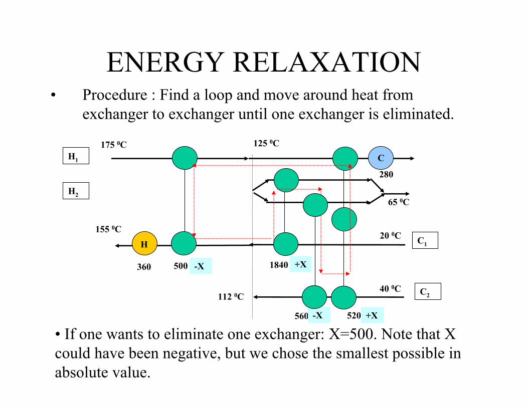
ENERGY RELAXATION • Procedure : Find a loop and move around heat from
exchanger to exchanger until one exchanger is eliminated.
155 0C
H1
H2
C2 112 0C
C1
125 0C
1840500360
20 0C
280
175 0C
40 0C
560 520
-X +X
-X +X
• If one wants to eliminate one exchanger: X=500. Note that X could have been negative, but we chose the smallest possible in absolute value.
H
C
65 0C

ENERGY RELAXATION • Result: Notice that the result is infeasible!!!
155 0C
H1
H2
C2 112 0C
C1
73 0C
2340360
20 0C
280
175 0C
40 0C
60 1020
108 0C
This exchanger is in violation of the minimum approach
45 0C
65 0C
65 0C65 0C
H
C

ENERGY RELAXATION • We use a path to move heat around to restore feasibility
73 0C
The value of X needed to restore feasibility is X=795
155 0C
H1
H2
C2 112 0C
C1
2340
H20 0C
280
175 0C
40 0C
60 1020
108 0C
45 0C
65 0C
65 0C65 0C
+X
+X
+X
-X
-X
360
C

ENERGY RELAXATION • Final Network
155 0C
H1
H2
C2 112 0C
C1
1545
H20 0C
1075
175 0C
40 0C
855 225
55 0C
45 0C
65 0C
65 0C65 0C
1155
C
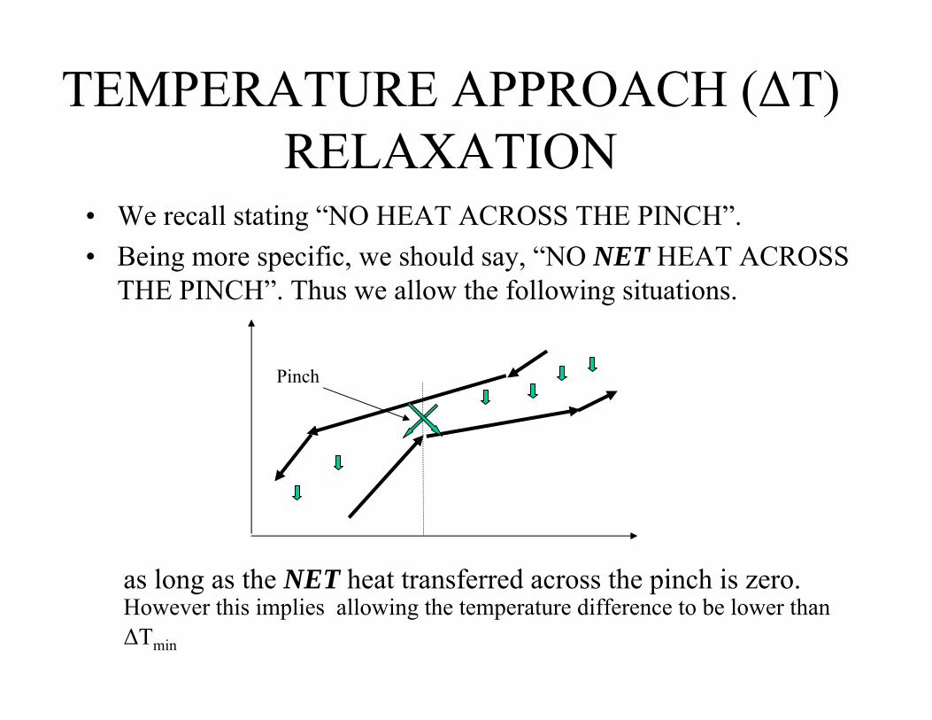
TEMPERATURE APPROACH (∆T) RELAXATION
Pinch
• We recall stating “NO HEAT ACROSS THE PINCH”. • Being more specific, we should say, “NO NET HEAT ACROSS
THE PINCH”. Thus we allow the following situations.
as long as the NET heat transferred across the pinch is zero. However this implies allowing the temperature difference to be lower than ∆Tmin

∆T RELAXATION• We thus define two types of Minimum Temperature Approach.
• HRAT: (Heat Recovery Approach Temperature): This is the ∆Tmin we use to calculate minimum utility.
• EMAT: (Exchanger Minimum Approach Temperature): This is the minimum approach we will allow in heat exchangers.
When EMAT< HRAT networks can have 1. less splitting 2. less number of units 3. No significant increase in the total area.

Consider the following problem
∆Tmin Hot Utility Cold Utility Pinch
20 (HRAT) 0.605 MW 0.525 MW 132 OC
13 (EMAT) 0.360 MW 0.280 MW 112 OC
Stream Type Supply T Target T F*Cp (oC) (oC) (MW oC-1)
H1 Hot 175 45 0.010
H2 Hot 125 65 0.040
C1 Cold 20 155 0.020
C2 Cold 40 112 0.015
∆T RELAXATION
We now consider HRAT=20 oC and EMAT= 13 oC. The corresponding minimum utility are:

We now consider that the difference (245 kW= 605 kW-360 kW) needs to go across the pinch of a design made using EMAT. Thus we first look at the solution of the pinch design method (PDM) for ∆Tmin =13 oC
PSEUDO-PINCH METHOD
45 0C
155 0C
H1
H2
C2
FCp=0.010
FCp=0.040
FCp=0.020
FCp=0.015
112 0C
C1
65 0C
125 0C
1840500360
20 0C
280
175 0C
40 0C
560 520
(*) Heat exchanger loads are in kW
H

To relax this network by 245 kW we extend the only heat exchanger above the pinch by this amount. We then proceed below the pinch as usual.
PSEUDO-PINCH METHOD
45 0C
155 0C
H1
H2
C2
FCp=0.010
FCp=0.040
FCp=0.020
FCp=0.015
112 0C
C1
65 0C
149.5 0C
1840255605
20 0C
310
175 0C
40 0C
735 345
(*) Heat exchanger loads are in kW
125 0C
112 0C
Note that the matching rules (FCp inequalities) can be somewhat relaxed.
H
C
215
C
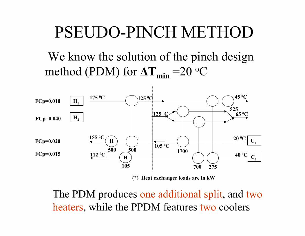
We know the solution of the pinch design method (PDM) for ∆Tmin =20 oC
PSEUDO-PINCH METHOD
45 0C
155 0C
H1
H2
C2
FCp=0.010
FCp=0.040
FCp=0.020
FCp=0.015 112 0C
C1
65 0C
1700500500
20 0C
525
175 0C
40 0C
700 275
(*) Heat exchanger loads are in kW
125 0C
105 0C
125 0C
105
The PDM produces one additional split, and two heaters, while the PPDM features two coolers
H
H
• No clear indication what to do when there is many hot streams above the pinch. How to distribute the difference in heat?
• Even if the above is clarified it is not practical for more than a few streams.
DIFFICULTIES IN THE PPDM METHOD

• One can use the Transshipment model fixing the level of hot utility and creating the intervals using EMAT instead of HRAT.
• More sophisticated methods add area estimation to the model (This has been called the Vertical model)
• The number of units can also be controlled and sophisticated techniques have been used to explore all the flowsheets with the same number of matches.
• Finally, once a flowsheet is obtained a regular optimization can be conducted.
• This will be explored in the next Part.
∆T RELAXATION USING AUTOMATIC METHODS

PART 7
MATHEMATICAL PROGRAMMING
APPROACHES

RECENT REVIEW PAPER
• Furman and Sahinidis. A critical review and annotated bibliography for Heat Exchanger Network Synthesis in the 20th Century. Ind. Eng. Chem. Res., 41 pp. 2335-2370, (2002).
(until 2000)
PINCH DESIGN METHOD
• It is a DECOMPOSITION approach (3 steps)– Perform Supertargeting and obtain the right HRAT,
the pinch (or pinches) and the minimum utility usage– Pick matches away from the pinch using the tick-off
rule– Evolve into higher energy consumption solutions by
loop breaking and adjusting loads on paths.

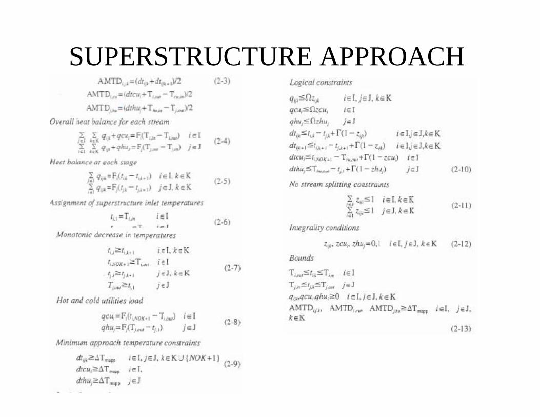
SUPERSTRUCTURE APPROACH
• CONCEPT: A single optimization model, if solved globally, provides all the answers simultaneously.
Superstructure of matches.

SUPERSTRUCTURE APPROACHPossible flow sheets embedded (recycles/by-passes excluded)

SUPERSTRUCTURE APPROACHPossible flow sheets embedded (continued)

SUPERSTRUCTURE APPROACHModel Constraints
Objective (no fixed costs)

SUPERSTRUCTURE APPROACH
ALTOUGH A ONE-STEP CONCEPT IT BECAME IN REALITY AN ITERATIVE PROCESS
– This is an MINLP formulation with which several researches have struggled. (MINLP methods could not be easily solved globally until recently (?).
– Therefore it needs some initial points.

SUPERSTRUCTURE APPROACH• Some Strategies to overcome the “curse of
non-convexity”
Many other methodologies attempted this goal (provide good initial points) like evolutionary algorithms, simulated annealing, etc.
Hasemy-Ahmady et al., 1999.

STAGE SUPERSTRUCTURE APPROACH
• With isothermal mixing. Yee and Grossmann (1990, 1998)
In the 90’s the mathematical programming/ superstructure approach emerged as the dominant methodology
Note on the side: This is a remarkable coming back to origins.
From Grossmann and Sargent (1978)

SUPERSTRUCTURE APPROACH
From Grosmann and Sargent (1978)
SUPERSTRUCTURE APPROACH

LATEST MILP APPROACH(Barbaro and Bagajewicz, 2005)
Counts heat exchangers units and shellsApproximates the area required for each exchanger unit or shellControls the total number of unitsImplicitly determines flow rates in splitsHandles non-isothermal mixingIdentifies bypasses in split situations when convenientControls the temperature approximation (HRAT/EMAT or ∆Tmin) when desiredAllows multiple matches between two streams

LATEST MILP APPROACH(Barbaro and Bagajewicz, 2005)
1 2 3 45 6
7 8
m
1 2 3 4 56 7 8 9
n
Hzijmq ,ˆ
zjnimq ,
Czijnq ,ˆ
istreamHot
jstreamCold
Transportation Model Approach

LATEST MILP APPROACH(Barbaro and Bagajewicz, 2005)
Heat Exchanger countingHz
ijmHz
ijm YK ,,ˆ ≥
Hzijm
Hzijm
Hzijm YYK ,
1,, 2ˆ
+−−≤
Hzijm
Hzijm YK ,,ˆ ≤
Hzijm
Hzijm
Hzijm YYK ,
1,,ˆ
+−≥
0ˆ , ≥HzijmK
First interval
Rest of intervals
1 2 3 4 5 6 7 8 9 10m 1 2 3 4 5 6 7 8 9 10m 1 2 3 4 5 6 7 8 9 10m
Hz,ijmY Hz,
ijmK Hz,ijmK̂
00010
0009
1018
0017
0016
0015
0014
0113
0002
0001
m
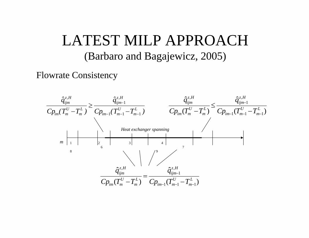
LATEST MILP APPROACH(Barbaro and Bagajewicz, 2005)
Flowrate Consistency
)(ˆ
)(ˆ
111
,1
,
Lm
Umim
Hzijm
Lm
Umim
Hzijm
TTCpq
TTCpq
−−−
−
−=
−
)TT(Cpq̂
)TT(Cpq̂
Lm
Umim
H,zijm
Lm
Umim
H,zijm
111
1
−−−
−
−≥
− )(ˆ
)(ˆ
111
,1
,
Lm
Umim
Hzijm
Lm
Umim
Hzijm
TTCpq
TTCpq
−−−
−
−≤
−
1 2 3 46 7
8 9
m
Heat exchanger spanning
PART 8
INDUSTRIAL IMPORTANCE OF USING THE RIGHT MODEL
Crude fractionation case study
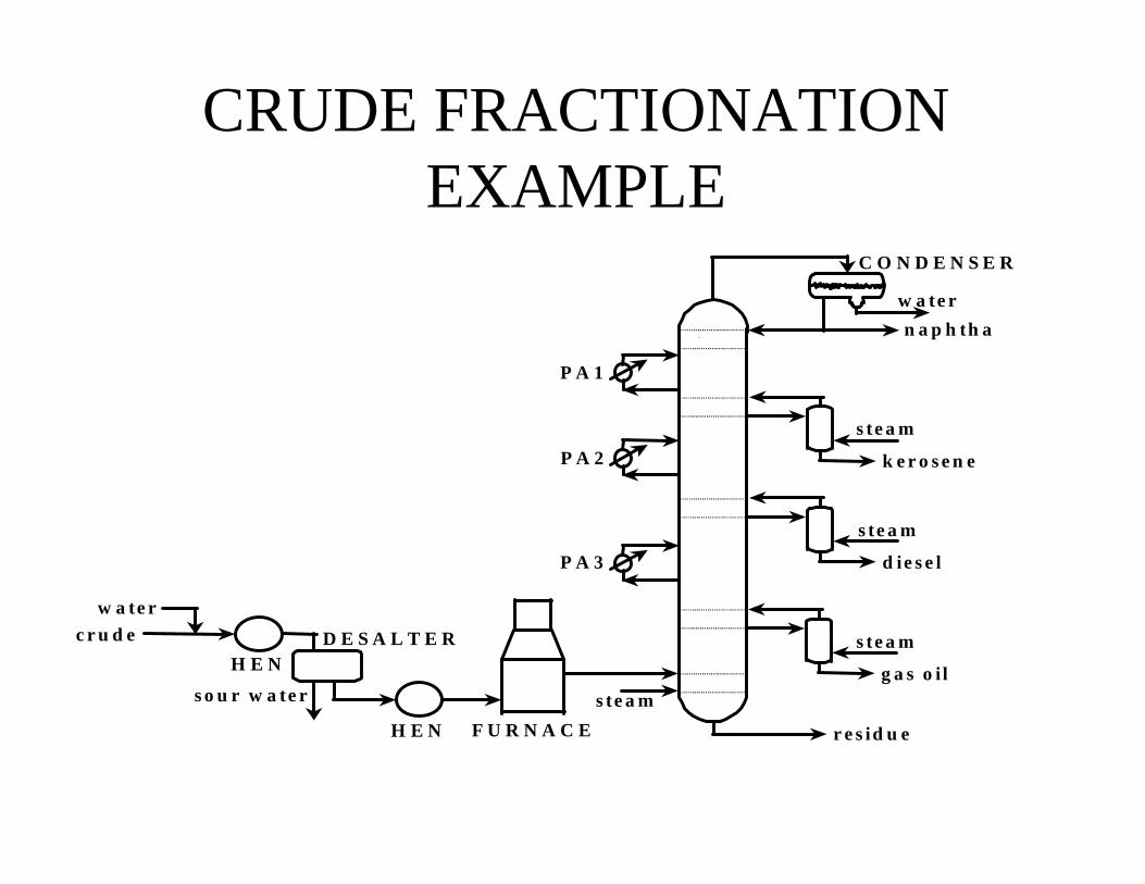
CRUDE FRACTIONATION EXAMPLE
c r u d ew a te r
H E N
H E N
D E S A L T E R
s o u r w a te r
F U R N A C Es te a m
s te a m
s te a m
s te a m
P A 3
P A 2
P A 1
k e r o s e n e
d ie s e l
g a s o i l
r e s id u e
n a p h th aw a te r
C O N D E N S E R

CRUDE FRACTIONATION EXAMPLELight Crude
0
50
100
150
200
250
300
350
400
0 50 100 150 200 250
Enthalpy (MW)
Tem
pera
ture
(o C
)
Heavy Crude
0
50
100
150
200
250
300
350
400
0 50 100 150 200
Enthalpy (MW)Te
mpe
ratu
re (C
)
Cooling water is already included in the graphs.
•The light crude exhibits what is called a continuous pinch.
•The heavy crude is unpinched.

CRUDE FRACTIONATION
MER network for the light crude.
Cooling water
DESALTER
C2
FURNACE
H4H9
H1
H10
H8
H2 H3 H7
H6
H5

CRUDE FRACTIONATION
MER network for the heavy crude.
Cooling water
DESALTER
C2
FURNACE
H6
H2
C1
H8
H7
H10H1
H5
H3H4

CRUDE FRACTIONATION
MER network efficient for both crudes.
DESALTER
C1
H10
H4
FURNACE
H1
H8
H2 H3 H7
H6
H5
H9
C2NOT USED FORHEAVY CRUDE
NOT USED FORLIGHT CRUDE
Cooling water

CRUDE FRACTIONATIONIt is clear from the previous results that efficient MER networks addressing multiple crudes can be rather complex and impractical.
Alternatives to the Pinch Design Method (PDM) are clearly needed.
This does not mean that the PDM fails all the time. It is still capable of producing good results in many other cases.

CRUDE FRACTIONATION EXAMPLE
We now illustrate the use of HRAT/EMAT procedures for the case of crude fractionation units.
We return to our example of two crudes. The problem was solved using mathematical programming. The networks have maximum efficiency for both crudes.
Only the vertical model and the control on the number of units was used. No variation in the matches was done (not really necessary in this case) and no further optimization was performed.

CRUDE FRACTIONATION
Solution for HRAT/EMAT = 20/10 oF
NOT USED FORHEAVY CRUDE
Cooling water
18 units18 units
DESALTER
C1
C2
FURNACE
H7H3
H8
H6
H1
H5H2
H4
H10
H9
NOT USED FOR HEAVY CRUDE
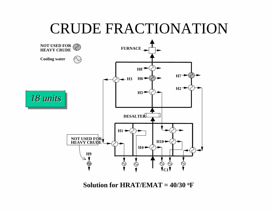
CRUDE FRACTIONATION
Solution for HRAT/EMAT = 40/30 oF
NOT USED FORHEAVY CRUDE
Cooling water
C1
NOT USED FORHEAVY CRUDE
FURNACE
H8
H6
H5
H7
H2
H10H4
H1
DESALTER
H9
H3
18 units18 units

CRUDE FRACTIONATION
Solution for HRAT/EMAT = 80/60 oF
NOT USED FORHEAVY CRUDECooling water
NOT USED FORHEAVY CRUDE
FURNACE
H8
H6
H7
H2
H10
H4
H1
C1
DESALTER
H9
H3
H517 units17 units

CRUDE FRACTIONATION
Combined Multiperiod Multiperiod+ Multip+Des.TempNetwork Model Desalt.Temp. +Higher HRAT
Operational 3.96 3.96 3.96 4.94Fixed 3.14 3.63 3.32 1.37Total 7.10 7.59 7.28 6.32
Cost, MM$/yrCost, MM$/yr
HRAT/EMAT 20/20 20/10 20/10 40/30
CRUDE FRACTIONATION EXAMPLE
We now illustrate the use of more sophisticated models that allow the control of splitting. These are essentially transshipment models that are able to control the level of splitting (something that regular transshipment models cannot do).

CRUDE FRACTIONATIONTwo branches unrestricted
23 units23 units
HRAT = 40 HRAT = 40 ooFFEMAT = 30 EMAT = 30 ooFF
FURNACE
H7
H6
H10
H4
H2
C1
DESALTER
H3
H5
H8
H1
H9
5% More Energy5% More EnergyConsumptionConsumption
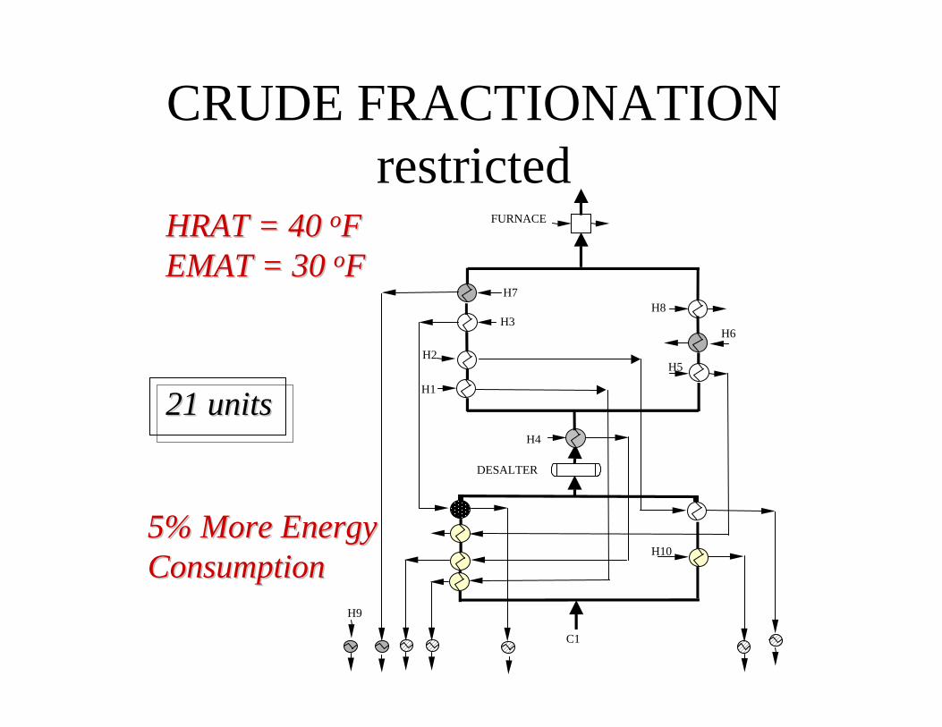
CRUDE FRACTIONATION restricted
21 units21 units
HRAT = 40 HRAT = 40 ooFFEMAT = 30 EMAT = 30 ooFF
FURNACE
H8
H6
H7
H2
H10
H4
H1
C1
DESALTER
H9
H3
H5
5% More Energy5% More EnergyConsumptionConsumption

CRUDE FRACTIONATION
Cost, MM$/yrCost, MM$/yr
Multiperiod Two-branch Two-branchModel Unrestricted Restricted
Operational 4.32 4.52 4.53Fixed 2.07 1.90 2.01Total 6.39 6.42 6.54
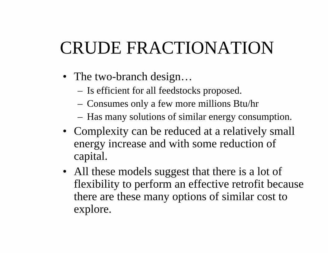
CRUDE FRACTIONATION• The two-branch design…
– Is efficient for all feedstocks proposed.– Consumes only a few more millions Btu/hr– Has many solutions of similar energy consumption.
• Complexity can be reduced at a relatively small energy increase and with some reduction of capital.
• All these models suggest that there is a lot of flexibility to perform an effective retrofit because there are these many options of similar cost to explore.

PART 9
RETROFITAND
TOTAL SITE INTEGRATION

RETROFITThe big question in trying to do a retrofit of a HEN is whether one really wants to achieve maximum efficiency.
Operating
Costs ($/yr)
Capital Investment ($)
Original System
HORIZON
Usually retrofits are too expensive and have a long payout.
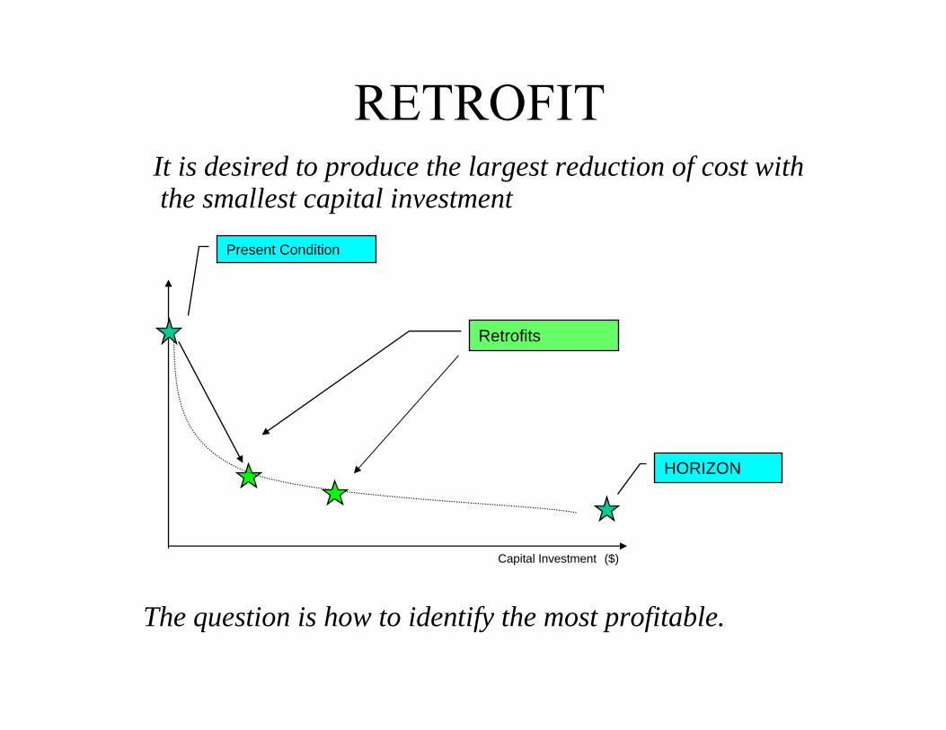
RETROFITIt is desired to produce the largest reduction of cost with the smallest capital investment
Capital Investment ($)
Present Condition
Retrofits
HORIZON
The question is how to identify the most profitable.
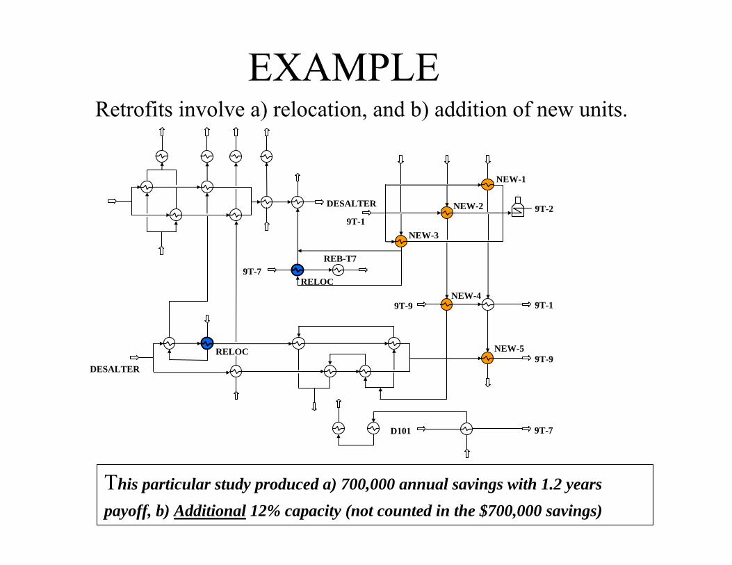
EXAMPLERetrofits involve a) relocation, and b) addition of new units.
NEW-1
NEW-2
NEW-3
REB-T7
DESALTER
NEW-49T-9 9T-1
9T-1
9T-7
NEW-5
DESALTER9T-9
9T-2
D101 9T-7
RELOC
RELOC
This particular study produced a) 700,000 annual savings with 1.2 years payoff, b) Additional 12% capacity (not counted in the $700,000 savings)

TYPES OF RETROFIT
• By inspection. Perform pinch design or pseudo pinch
design and determine heat exchangers to add
• Systematic methods using tables and graphs exist
They are outside the scope of this course.
• Mathematical programming approaches also exist but
they have not passed the test of usability and
friendliness
RECENT WORK ON RETROFIT• Asante, N. D. K.; Zhu, X. X. An Automated and Interactive Approach for Heat
Exchanger Network Retrofit. Chem.Eng. Res. Des. 75 (A), 349-360 (1997).
• Briones, V.; Kokossis, A. C. Hypertargets: A Conceptual Programming Approach
for the Optimisation of Industrial Heat Exchanger Networks II. Retrofit Design.
Chem. Eng. Sci. 54, 541-561 (1999).
• Barbaro, Bagajewicz, Vipanurat, Siemanond. MILP formulation for the Retrofit of
Heat Exchanger Networks. Proceedings of Pres 05. (2005)

TOTAL SITE INTEGRATION • USE OF GRAND COMPOSITE CURVES TO PLACE UTILITIES.
Pockets are eliminated and curves are shifted
∆H
Plant 1
∆H
Plant 2

TOTAL SITE INTEGRATION • Site sink and source profiles are constructed.
Energy integration is performed by placing utilities. We will see how this method can be wrong.
∆H
Source ProfileSink Profile
Overlap region. These are savings.
HP SteamLP Steam

TOTAL SITE INTEGRATION• Consider two plants. We would like to know under what
conditions one can send heat from one plant to the other.
P L A N T 2P L A N T 1C O M B IN E D
P L A N T
P in c h P o in tP la n t 2
P in c h P o in tP la n t 1
A b o v e b o th p in c h e s
B e tw e e n p in c h e s
B e lo w b o th p in c h e s
P o ss ib le L o c a tio n o f
P in c h

TOTAL SITE INTEGRATION
Effective integration takes place between pinches.
From where plant 2 is heat source to where plant 1 is heat sink.
T
Pinch 1
U1,min- QT
QT
W1,min
Pinch 2
W2,min- QT
U2,min

TOTAL SITE INTEGRATION
Integration outside the inter pinch region leads to no effective savings.
T
Pinch 1
U1,min- QT
QT
W1,min
Pinch 2
W2,min
U2,min + QT

GRAND COMPOSITE CURVES
-12
-1
-15
-2
2
6 = 18 - 12
5 = 6 - 1
0 = 5 - 15 + 10
0 = 0 - 2 + 2
18 = 30 - 12
-19
-1
10
5
1
1 = 20 - 19
0 = 1 - 1
0 = 10 - 10
3 = 0 + 5 - 2
20 = 20
10
2 = 2 4 = 3 + 1
PLANT 1 PLANT 2
2
Pinch
Pinch

GRAND COMPOSITE CURVES
40
60
80
100
120
140
-20 -15 -10 -5 0 5 10 15 20
Enthalpy
Tem
pera
ture
Maximum possible savings
Plant 1Plant 2

ASSISTED HEAT TRANSFER
-7
5
-15
-3
3
0 = 7 - 7
1 = 0 + 5 - 4
0 = 1 - 15 + 14
0 = 0 - 3 + 3
7 = 20 + 4 - 17
-10
-10
14
10
5
6 = 16 - 10
0 = 6 - 10 + 4
0 = 14 - 14
7 = 0 + 10 - 3
16 = 20 - 4
14
3 = 3 12 = 7 + 5
4
3
PLANT 1 PLANT 2
Pinch
Pinch
If heat is not transferred above the two pinches only 13 of the maximum 17 can be saved.

ASSISTED HEAT TRANSFER
40
60
80
100
120
140
-10 -5 0 5 10 15 20 25 30
Enthalpy
Tem
pera
ture
Maximum possible savings
Plant 1
Plant 2
AssistedTransfer Pocket
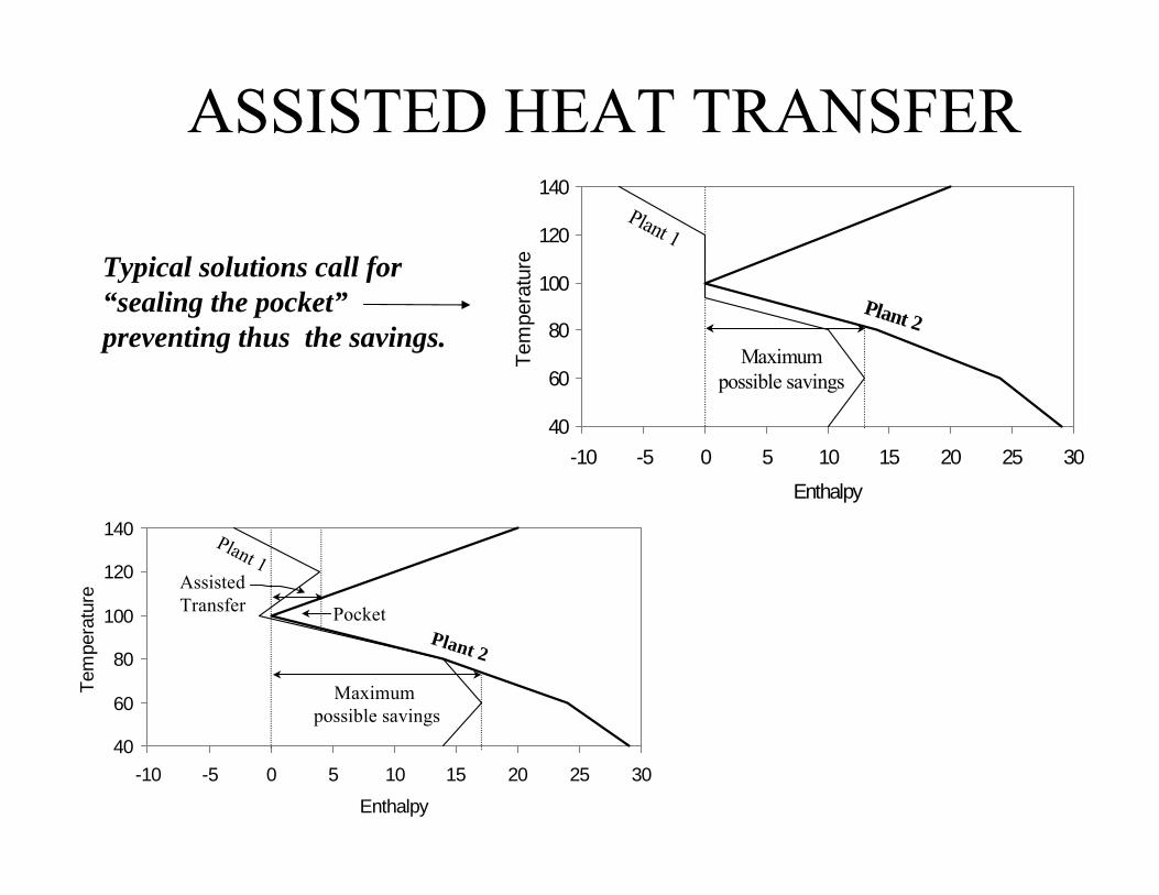
ASSISTED HEAT TRANSFER
Typical solutions call for “sealing the pocket”preventing thus the savings.
40
60
80
100
120
140
-10 -5 0 5 10 15 20 25 30
Enthalpy
Tem
pera
ture
Maximum possible savings
Plant 1
Plant 2
AssistedTransfer Pocket
40
60
80
100
120
140
-10 -5 0 5 10 15 20 25 30Enthalpy
Tem
pera
ture
Maximumpossible savings
Plant 2
Plant 1

HEAT EXCHANGER NETWORKSHeat Exchanger networks should be such that both plants can work at maximum efficiency when integrated and when they stand alone.
We now show a result of a case study. An integration between a Crude unit (heat sink ) and an FCC unit (heat source).
Plant 1: Crude Unit
H3 H4 H9
Direct Integration(two stream circuits)
H8
H5 H6 H7
Plant 2: FCC Unit
CW
H12
H13 H11 H10 H15 H14
C1
H1
CW
H2
Above the Pinch
Below the Pinch Additional heat exchangersused during integration
Original HENPinch location
C2
Savings 1,000,000 $/year
Utility (MMBtu/hr)Heating Cooling
No Integration 252.9 147.7Direct Integration 201.4 96.2

TOTAL SITE INTEGRATION Multiple plants can also be analyzed. We show below one example of such studies.
•Alternative solutions exists.
•Grand composite curves cannot be used anymore.
P L A N T 3(C & F )
P L A N T 2(T r iv e d i)
P L A N T 1(T e s t C a s e # 2 )
P L A N T 4(4 s p 1 )
9 8 .3
5 2 .91 2 0 .7
1 0 4 .5
1 0 7 .5
3 0 0 ° C
2 4 9 ° C
2 0 0 ° C
1 6 0 ° C
9 0 ° C
4 0 ° C
0 2 5 4 .9 4 2 6 .4 1 2 8
4 0 5 8 1 .1 1 9 9 5 .5 3 1 .1
P L A N T 3(C & F )
P L A N T 2(T r iv e d i)
P L A N T 1(T e s t C a s e # 2 )
P L A N T 4(4 s p 1 )
9 8 .3
5 2 .91 2 0 .7
1 0 4 .5
1 0 7 .5
3 0 0 ° C
2 4 9 ° C
2 0 0 ° C
1 6 0 ° C
9 0 ° C
4 0 ° C
0 2 5 4 .9 4 2 6 .4 1 2 8
4 0 5 8 1 .1 1 9 9 5 .5 3 1 .1
P L A N T 3(C & F )
P L A N T 2(T r iv e d i)
P L A N T 1(T e s t C a s e # 2 )
P L A N T 4(4 s p 1 )
P L A N T 3(C & F )
P L A N T 2(T r iv e d i)
P L A N T 1(T e s t C a s e # 2 )
P L A N T 4(4 s p 1 )
9 8 .3
5 2 .91 2 0 .7
1 0 4 .5
1 0 7 .5
3 0 0 ° C
2 4 9 ° C
2 0 0 ° C
1 6 0 ° C
9 0 ° C
4 0 ° C
3 0 0 ° C
2 4 9 ° C
2 0 0 ° C
1 6 0 ° C
9 0 ° C
4 0 ° C
0 2 5 4 .9 4 2 6 .4 1 2 8
4 0 5 8 1 .1 1 9 9 5 .5 3 1 .1

FUTURE TRENDS• Mathematical programming will be the dominant
tool. • Software companies are struggling to make the
proper choice of existing methods for each case and most important numerically reliable.
• The best option for the time being is to intelligently interact with experts while using existing software.