part ii complex economic dynamics: agent-based and analytical

This file is to be used only for a purpose specified by Palgrave Macmillan, such as checking proofs, preparing an index, reviewing, endorsing or planning coursework/other institutional needs. You may store and print the file and share it with others helping you with the specified purpose, but under no circumstances may the file be distributed or otherwise made accessible to any other third parties without the express prior permission of Palgrave Macmillan. Please contact [email protected] if you have any queries regarding use of the file.

AOKI-V2: “9781137_034205_04_CHAP02” — 2012/7/10 — 14:22 — PAGE 31 — #1

Part IIComplex Economic Dynamics:Agent-based and Analytical Models

PROOF

AOKI-V2: “9781137_034205_04_CHAP02” — 2012/7/10 — 14:22 — PAGE 32 — #2

PROOF

AOKI-V2: “9781137_034205_04_CHAP02” — 2012/7/10 — 14:22 — PAGE 33 — #3

2The Dynamics of Pure MarketExchangeHerbert GintisSanta Fe Institute, USA and Central European University, Hungary

The problem of a rational economic order is determined precisely by the factthat the knowledge of the circumstances of which we must make use neverexists in concentrated or integrated form, but solely as the dispersed bits ofincomplete and frequently contradictory knowledge which all the separateindividuals possess. (F.A. Hayek 1945: 519)

2.1 Introduction

Adam Smith (2000 [1759]) envisioned a decentralized economy that sustains anefficient allocation of resources through the ‘invisible hand’ of market competi-tion. Smith’s vision was formalized by LéonWalras (1954 [1874]), and a proof ofexistence of equilibrium for a simplified version of the Walrasian economy wasprovided by Wald (1951 [1936]). Soon after, Debreu (1952), Arrow and Debreu(1954), Gale (1955), Nikaido (1956), McKenzie (1959), Negishi (1960), and oth-ers contributed to a rather complete proof of the existence of equilibrium inWalrasian economies. Such economies are particularly attractive because theycapture the basic structural characteristics of market economies, and becausea Walrasian equilibrium is Pareto-efficient (Arrow 1951; Debreu 1951, 1954;Hurwicz 1960).The question of stability of theWalrasian economywas a central research focus

in the years immediately following the existence proofs (Arrow and Hurwicz,1958, 1959, 1960; Arrow, Block and Hurwicz, 1959; Nikaido 1959; McKenzie,1960; Nikaido and Uzawa 1960; Uzawa 1960). Themodels investigated assumedthat out of equilibrium, there is a system of public prices shared by all agents, thetime rate of change of prices being a function of excess demand. The public pricesystem was implemented by a single agent (the ‘auctioneer’) acting outside theeconomy to update prices in the current period on the basis of the current pat-tern of excess demand, using a process of ‘tâtonnement’, as was first suggestedby Walras (1954 [1874]) himself.

33

PROOF

AOKI-V2: “9781137_034205_04_CHAP02” — 2012/7/10 — 14:22 — PAGE 34 — #4

34 H. Gintis

The quest for a general stability theoremwas derailed by Herbert Scarf’s simpleexamples of unstable Walrasian equilibria (Scarf, 1960). There were attemptssoon after to continue the analysis of tâtonnement by adding trading out ofequilibrium (Uzawa 1959, 1961, 1962; Negishi 1961; Hahn 1962; and Hahnand Negishi 1962), but with only limited success.General equilibrium theorists in the early 1970s harbored some expectation

that plausible restrictions on utility functions might entail stability, becausegross substitutability was known to imply global stability (Arrow et al., 1959)and gross substitutability was known to hold for Cobb–Douglas and manyother utility functions (Fisher, 1999). However, gross substitutability is not aproperty of constant elasticity of substitution (CES) and more general utilityfunctions. Moreover, Sonnenschein (1973), Mantel (1974, 1976), and Debreu(1974) showed that any continuous function, homogeneous degree zero inprices, and satisfying Walras’ Law, is the excess demand function for someWalrasian economy.However, Hahn and Negishi (1962) showed that if out-of-equilibrium trade

is permitted and the so-called Hahn condition obtains, then the Walrasianequilibrium is stable under tâtonnement. The Hahn condition says thatmarkets are sufficiently informationally complete that if there is aggregateexcess demand then no individual experiences excess supply, and if thereis aggregate excess supply, then no individual experiences excess demand.Fisher (1983) significantly broadened this model and proved stability assum-ing a expectational condition (‘no favorable surprise’) that should logi-cally hold in any Walrasian equilibrium, plus a weakened Hahn condition,according to which lower-price sellers realize their plans before higher-pricesellers do.Nevertheless, surveying the state of the art some quarter-century after Arrow

and Debreu’s seminal existence theorems, Fisher (1983) concluded that littleprogress had been made toward a cogent model of Walrasian market dynam-ics. More recent studies have shown that the tâtonnement dynamic is stableonly under extremely stringent conditions (Kirman, 1992). Indeed, chaos inprice movements is the generic case for the tâtonnement adjustment processes(Saari, 1985; Bala and Majumdar, 1992). Saari (1995) and others have shownthat the information needed by a price adjustment mechanism that can ensurestability include virtually complete knowledge of all cross-elasticities of demandin addition to excess demand quantities.It is now more than another quarter-century since Fisher’s seminal contri-

butions, but it remains the case that, despite the centrality of the generalequilibrium model to economic theory, we know nothing systematic aboutWalrasian market dynamics in realistic settings. We show that when the mar-ket system is modeled as a Markov process rather than a system of first-orderdifferential equations, a powerful analytical dynamic emerges.

PROOF

AOKI-V2: “9781137_034205_04_CHAP02” — 2012/7/10 — 14:22 — PAGE 35 — #5

The Dynamics of Pure Market Exchange 35

2.2 A Markov process primer

We will model the Walrasian economy as a Markov process, starting for illus-trative purposes with a very elementary and purely didactic example. Our goalis to show that even a very simple finite Markov process may have too manystates to permit an analytical solution, yet the global properties of the modelare easily understood.Consider an economy with k goods, each of which could serve equally well

as a money good for the economy. Suppose there are n agents in the economy,and in each period, each agent is willing to accept exactly one good as money.Suppose further that in each period, one agent switches from his own preferredmoney to that of another randomly encountered agent. We can describe thestate of the economy as a k-vector (w1. . .wk), where wi is the number of agentswho accept good i as money. The total number of states in the economy isthus the number of different ways to distribute n indistinguishable balls (the nagents) into k distinguishable boxes (the k goods), which is C(n+ k− 1,k− 1),where C(n,k) = n!/(n−k)!k! is the number of ways to choose k objects from a setof n objects. To verify this formula, write a particular state in the form

s= x. . .xAx. . .xAx. . .xAx. . .x

where the number of x’s before the first A is the number of agents choosing good1 as money, the number of x’s between the (i−1)th A and the ith A is the numberof agents choosing good i as money, and the number of x’s after the final A isthe number agents choosing good k as money. The total number of x’s is equalto n, and the total number of A’s is k− 1, so the length of s is n+ k− 1. Everyplacement of the k−1 A’s represents particular state of the system, so there areC(n+ k−1,k−1) states of the system.For instance, if n= 100 and k= 10, then the number of states S in the system

is S = C(109,9) = 4,263,421,511,271. Suppose in each period two agents arerandomly chosen and the first agent switches to using the second agent’s moneygood as his own money good (the two money goods may in fact be the same).This gives a determinate probability pij of shifting from one state i of the systemto any other state j. The matrix P = {pij} is called a transition probability matrix,and the whole stochastic system is called a Markov process. The Markov processis finite because it has a finite number of states.What is the long-run behavior of this Markov process? Note first that if we

start in state i at time t = 0, the probability p(2)

ij of being in state j in period t = 2is simply

p(2)

ij =S∑k=1

pikpkj = (P2)ij. (1)

PROOF

AOKI-V2: “9781137_034205_04_CHAP02” — 2012/7/10 — 14:22 — PAGE 36 — #6

36 H. Gintis

This is true because to be in state j at t = 2 the system must have been in somestate k at t = 1 with probability pik, and the probability of moving from k toj is just pkj. This means that the two-period transition probability matrix forthe Markov process is just P2, the matrix product of P with itself. By similarreasoning, the probability of moving from state i to state j in exactly r periods,is Pr . Therefore, the time path followed by the system starting in state s0 = i attime t = 0 is the sequence s0,s1, . . ., where

P[st = j|s0 = i] = (Pt )ij = p(t)ij .

The matrix P in our example has S2 ≈ 1.818× 1015 entries. The notion of cal-culation Pt for even small t is quite infeasible. There are ways to reduce thecalculations by many orders of magnitude (Gintis, 2009, Ch. 13), but eventhese are completely impractical with so large a Markov process.Nevertheless, we can easily understand the dynamics of this Markov process.

We first observe as that if the Markov process is ever in the state

sr∗ = (01, . . .,0r−1,nr ,0r+1. . .0k),

where all n agents choose good r money, then sr∗ will be the state of the systemin all future periods. We call such a state absorbing. There are clearly only kabsorbing states for this Markov process. We next observe that from any non-absorbing state s, there is a strictly positive probability that the system movesto an absorbing state before returning to state s. For instance, suppose wi = 1 instate s. Then there is a positive probability that wi increases by 1 in each of thenext n−1 periods, so the system is absorbed into state si∗ without ever returningto state s. Now let ps > 0 be the probability that Markov process never returnsto state s. The probability that the system returns to state s at least q times isthus at most (1− ps)q. Since this expression goes to zero as q→ ∞, it followsthat state s appears only a finite number of times with probability one. We call s atransient state.Because state s in the previous argument was an arbitrary non-absorbing state,

it follows that all non-absorbing states are transient. It is also clear that with prob-ability one there will be some period t such that no transient state reappearsafter period t . This means that with probability one the system is absorbed intoone of the k absorbing states, from which it never emerges. Inevitably in thissystem one good emerges as the money good for the economy.We can in fact often calculate the probability that a system starting out with

wr agents choosing good r as money, is absorbed by state sr∗. Let us think ofthe Markov process as that of k gamblers, each of whom starts out with anintegral number of k coins, there being n coins in total. The gamblers representthe goods and their coins are the agents who choose that good for money. Wehave shown that in the long run, one of the gamblers will have all of the coins,

PROOF

AOKI-V2: “9781137_034205_04_CHAP02” — 2012/7/10 — 14:22 — PAGE 37 — #7


with probability one. Suppose the game is fair in the sense that in any perioda gambler with a positive number of coins has an equal chance to increase ordecrease his wealth by one coin. Then the expectedwealth of a gambler in periodt + 1 is just his wealth in period t . Similarly, the expected wealth E[wt ′ |wt ] inperiod t ′ > t of a gambler whose wealth in period t is wt is E[wt ′ |wt ] = wt . Thismeans that if a gambler starts out with wealth w> 0 and he wins all the coinswith probability qw, then w= qwn, so the probability of being the winner is justqw =w/n.We now can say that this Markov process, despite its enormous size, can be

easily described as follows. Suppose the process starts with wr = w. Then ina finite number of time periods, the process will be absorbed into one of thestates s1∗ , . . .,sk∗, and the probability of being absorbed into state sr∗ is w/n. Asit turns out, this description of a finite Markov process is completely general,except for a few technical points. In general, however, the process will not beabsorbed into a single state, but rather into what is called an irreducible Markovsubprocess, making transitions among a number of states, called communicatingrecurrent states. If the process is aperiodic, the fraction of time it is in each ofthese recurrent states state forms a probability distribution called the stationarydistribution of the ‘absorbing’ Markov subprocess. If the process is periodic, itcan be conveniently subdivided into a number of aperiodic subprocesses, eachwith a stationary distribution.

2.3 From differential equations to Markov processes

A plausible model of market dynamics should reflect two fundamental aspectsof market competition. First, trades must be bilateral with separate budgetequations for each transaction (Starr, 1972). The second is that in a decentral-ized market economy out of equilibrium, there is no price vector for the economyat all. The assumption that there is a system of prices that are common knowl-edge to all participants (we call these public prices) is plausible in equilibrium,because all agents can observe these prices in the marketplace. However, out ofequilibrium there is no vector of prices determined by market exchange. Rather,assuming Bayesian rational agents, every agent has a subjective prior concern-ing prices, based on personal experience, that the agent uses to formulate andexecute trading plans.Consider, for instance, the wage rate for a particular labor service. In equi-

librium, this price may be common knowledge, but out of equilibrium, everysupplier of this service must have an estimate of the probability of selling hisservice as a function of his offer price. The supplier, if Bayesian rational, willhave a subjective prior representing the shape of the demand function forthe service. This prior will determine whether the supplier accepts a particu-lar wage offer, or rejects the offer and continues searching for a better offer. The

PROOF

AOKI-V2: “9781137_034205_04_CHAP02” — 2012/7/10 — 14:22 — PAGE 38 — #8

38 H. Gintis

information needed to form this prior includes the distribution of subjectivepriors of demanders for the labor service, while the subjective prior of eachdemander will depend in a similar manner on the distribution of subjectivepriors of suppliers of the service. Thus in this case information is not sim-ply asymmetrically distributed, but rather is effectively indeterminate, sincethe supply schedule depends on suppliers’ assessment of demand conditions,and the demand schedule depends on demanders’ assessment of supply sched-ules. The conditions under which each agent’s choice is a best response tothe others’, even assuming common knowledge of rationality and commonknowledge of the Markov process (which in this case is the game in which theplayers are engaged), are quite stringent and normally not present (Aumannand Brandenburger, 1995).In analyzing market disequilibrium, we must thus assume that each agent’s

subjective prior includes a vector of private prices that is modified adaptivelythrough the exchange experience. The admissible forms of experience in adecentralizedmarket economy are those that result from observing the behaviorof trading partners. This experience is the sole basis for a trader’s updating hisprivate price vector, and equilibrium can be achieved only if plausible modelsof inference and updating lead private prices to converge to equilibrium prices(Howitt and Clower, 2000).In the interest of simplicity in dealing with a daunting problem that has defied

solution for more than a century, we will assume that there are no institutionsother than markets where individuals congregate to exchange their wares, thereare no forms of wealth other than agents’ production goods, all transactionstake place in the current period, so there is no intertemporal planning, andthere is no arbitrage beyond that which can be executed by an agent engagedin a series of personal trades using no information save that acquired throughpersonal trading experience.If we can show stability under these conditions (which we can) we then know

that trader information concerning macro aspects of the economy plays noessential role in achieving market equilibrium, and indeed may well have adestabilizing effect (Gintis, 2007).It follows logically that in so simple a market system with rational actors

but no public institutions, expectations are purely adaptive. The ‘rational expec-tations’ notion that agents know the global structure of the economy and usemacroeconomic information to form accurate expectations is not plausible inthe decentralized context. This conclusion may, of course, require revision in amodel with an institutional structure that creates public information, such as acredible government or national bank.An appropriate candidate for modeling the Walrasian system in disequilib-

rium is aMarkov process. The states of the process are vectorswhose componentsare the states of individual agents. The state of each agent includes his holding

PROOF

AOKI-V2: “9781137_034205_04_CHAP02” — 2012/7/10 — 14:22 — PAGE 39 — #9


of each good, an array of parameters representing his search strategies for buyingand selling, parameters representing his linkage to others in a network of traders,and finally his vector of private prices, which the agent uses to evaluate tradingoffers.If state si has a positive probability of making a transition to state sj in a

finite number of periods (i.e., p(t)ij > 0 for some positive integer t), we say sicommunicates with sj. If all states in a Markov process communicate with eachother, we say the process is irreducible. We cannot assume a Markov model ofa Walrasian system is irreducible because, as in our elementary example above,where a good inevitably emerges as money, the states of the system with onegood as money will not communicate with the states where a different goodis money.The Markov model of a Walrasian economy is finite if we assume there are a

finite number of agents, a finite number of goods, a minimum discernible quan-tity of each good, and a finite inventory capacity for each good. A strictly positiveprobability of remaining in the same state for an agent then ensures that theMarkov process is finite if aperiodic. Assuming for the moment that the Markovprocess is irreducible, being both and aperiodic implies the Markov process isergodic (Feller, 1950), which means has a stationary distribution expressing thelong-run probability of being in each state of the system, irrespective of itsinitial state.We may not care about individual states of the process, but rather about

certain aggregate properties of the system, including the mean and standarddeviation of prices, and the aggregate pattern of excess demand. As we shall see,the ergodic theorem ensures that under appropriate conditions these aggregateshave determinate long-term stationary distributions.

The Ergodic Theorem: Consider an n-state aperiodic and irreducible Markovprocesswith transitionmatrix P, so the t-period transition probabilities are givenby P(t) =Pt . Then there is probability distribution u= (u1, . . .,un) over the states oftheMarkov processwith strictly positive entries that has the following propertiesfor j= 1, . . .,n:

uj = limt→∞

p(t)ij for i= 1, . . .,n (2)

uj =n∑i=1

uipij (3)

We call u the stationary distribution of the Markov process.Equation (3) says that with probability one, uj is the long-run frequency of

state sj in a realization {st } = {s0,s1, . . .} of the Markov process. Also, this fre-quency is strictly positive and independent from the starting state s0 = si. By awell-known property of convergent sequences, (3) implies that uj is also with

PROOF

AOKI-V2: “9781137_034205_04_CHAP02” — 2012/7/10 — 14:22 — PAGE 40 — #10

40 H. Gintis

probability one the limit of the average frequency of sj from period t onwards,for any t . This is in accord with the general notion that in an ergodic dynamicalsystem, the equilibrium state of the system can be estimated as an historicalaverage over a sufficiently long time period (Hofbauer and Sigmund, 1998).Equation (3) is the renewal equation governing stationary distribution u. It

asserts that in the long run, the probability of being in state sj is the sum over iof the probability that it was in some state si in the previous period, multipliedby the probability of a one-period transition from state si to state sj, independentfrom the initial state of the realization {st } = {s0,s1, . . .}.A Markov process thus has only a one-period ‘memory.’ However, we can

consider a finite sequence of states {st−l,st−l+1, . . .,st } of the Markov processof fixed length l as a single state, the process remains Markov and has as anl-period ‘memory.’ Because any physically realized memory system, includingthe human brain, has finite capacity, the finiteness assumption imposes noconstraint on modeling systems that are subject to physical law.To see this, suppose a Markov process has transition matrix P = {pij} and con-

sider two-period states of the form ij. We define the transition probability ofgoing from ij to kl as

pij,kl ={pj,l j= k0 j �= k, (4)

This equation says that ij represents ‘state si in the previous period and state sj inthe current period.’ It is easy to check that with this definition the matrix {pij,kl}is a probability transition matrix, and if {u1, . . .,un} is the stationary distributionassociated with P, then

uij = uipi,j (5)

defines the stationary distribution {uij} for {pij,kl}. Indeed, we have

limt→∞

p(t)ij,kl = limt→∞

p(t−1)

j,k pk,l = ukpk,l = ukl

for any pair-state kl, independent from ij. We also have, for any ij,

uij = uipi,j =∑k

ukpk,ipi,j =∑k

ukipi,j =∑kl

uklpkl,ij. (6)

It is straightforward to show that pairs of states of P correspond to single statesof {pij,kl}. These two equations imply the ergodic theorem for {pij,kl} becauseequation 5 implies {uij} is a probability distribution with strictly positive entries,

PROOF

AOKI-V2: “9781137_034205_04_CHAP02” — 2012/7/10 — 14:22 — PAGE 41 — #11


and we have the defining equations of a stationary distribution; for any pair-state ij,

ukl = limt→∞

p(t)ij,kl (7)

uij =∑kl

uklpkl,ij. (8)

An argument by induction extends this analysis to any finite number ofsequential states of P.An important question is the nature of collections of states of a finite Markov

process. For instance, we may be interested in total excess demand for a goodwithout caring how this breaks down among individual agents. From the caseof two states j and k it will be clear how to generalize to any finite number. Letus make being in either state j or in state k into a new macro-state m. If P isthe transition matrix for the Markov process, the probability of moving fromstate i to state m is just Pim = Pij + Pik. If the process is ergodic with stationarydistribution u, then the frequency of m in the stationary distribution is justum = uj+uk. Then we have

um = limt→∞

Pnim (9)

um =∑i

ui pim (10)

However, the probability of a transition from m to a state i is given by

Pmi = uj pji+uk pki. (11)

Now suppose states j and k are interchangeable in the sense that pji = pki for allstates i. Then (7) implies

ui =∑rur pri, (12)

where r ranges over all states except j and k, plus the macro-state m. In otherwords, if we replace states j and k by the single macro-state m, the resultingMarkov process has one fewer state, but remains ergodic with the same sta-tionary distribution, except that um = uj +uk. A simple argument by inductionshows that any number of interchangeable states can be aggregated into a singlemacro-state in this manner.More generally, wemay be able to partition the states ofM into cellsm1, . . .,ml

such that, for any r=1, . . ., l and any states i and j ofM , i and j are interchangeablewith respect to each mk. When this is possible, then m1, . . .,ml are the states ofa derived Markov process, which will be ergodic if M is ergodic.For instance, in a particular market model represented by an ergodic Markov

process, wemight be able to use a symmetry argument to conclude that all states

PROOF

AOKI-V2: “9781137_034205_04_CHAP02” — 2012/7/10 — 14:22 — PAGE 42 — #12

42 H. Gintis

with the same aggregate demand for a particular good are interchangeable. Ifso, we can aggregate all states with the same total excess demand for this goodinto a single macro-state, and the resulting system will be an ergodic Markovprocess with a stationary distribution. In general, this Markov process will havemany fewer states, but still far too many to permit an analytical derivation ofthe stationary distribution.

2.4 The structure of finite aperiodic Markov processes

If a Markov process is finite and aperiodic but is not irreducible, its states can bepartitioned into subsets Str , S1, . . .Sk, where every state s∈ Str is transient, meaningthat for any realization {st } of the Markov process, with probability one thereis a time t such that s �= st+t ′ for all t ′ = 1,2, . . .; i.e., s does not reappear in {st }after time t . It follows that also with probability 1 there is a time t such that nomember of Str appears after time t . A non-transient state is called recurrent, forit reappears infinitely often with probability one in a realization of the Markovprocess.If si is recurrent and communicates with sj, then sj is itself recurrent and

communicates with si. For if j does not communicate with si, then every timesi appears, there is a strictly positive probability, say q > 0 that it will neverreappear. The probability that si appears k times is thus at most (1− q)k, so sireappears an infinite number of times with probability zero, and hence is notrecurrent. If sj communicates with si, then sj must be recurrent, as can be provedusing a similar argument.It follows that communication of states is an equivalence relation over the

recurrent states of the Markov process. We define S1, . . .Sk to be the equivalenceclasses of the recurrent states of the Markov process with respect to this equiv-alence relation. It is clear that the restriction of Markov process to any one ofthe Sr , r = 1, . . .,k is an ergodic Markov process with a stationary distribution.Moreover, if si ∈ Str , there is a probability distribution qi over {1, . . .,k} such thatqir is the probability, starting in si, the Markov process will eventually enter Sr ,from which it will, of course, never leave. Thus for an arbitrary finite, aperiodicMarkov process with transition matrix P = {pij}, we have the following.Extended Ergodic Theorem: LetM be a finite aperiodic Markov process. Thereexists a unique partition {Str ,S1, . . .,Sk} of the states S of M , a probability distri-bution ur over Sr for r = 1, . . .,k, such that uri > 0 for all i ∈ Sr , and for each i ∈ Str ,there is a probability distribution qi over {1, . . .,k} such that for all i, j = 1, . . .,nand all r = 1, . . .k, we have

uij = limt→∞

P(t)ij ; (13)

urj = uij if i, j ∈ Sr ; (14)

PROOF

AOKI-V2: “9781137_034205_04_CHAP02” — 2012/7/10 — 14:22 — PAGE 43 — #13


urj =∑i∈Sruri pij for j ∈ Sr ; (15)

uij = qirurj if si ∈ Str and sj ∈ Sr . (16)

uij = 0 if sj ∈ Str . (17)∑j

uij = 1 for all i= 1, . . .,n. (18)

For a Markov process with few states, there are well-known methods for solvingfor the stationary distribution (Gintis, 2009, Ch. 13). However, for systems witha large number of states, these methods are impractical. Rather, we here create acomputermodel of theMarkov process, and ascertain empirically the dynamicalproperties of the irreducible Markov subprocesses. We are in fact only interestedin measuring certain aggregate properties of the subprocess rather than theirstationary distributions. These properties are the long-run average price andquantity structure of the economy, as well as the short-run volatility of pricesand quantities and the efficiency of the process’s search and trade algorithms.It is clear from the quasi-ergodic theorem that the long-term behavior of anany realization of aperiodic Markov process is governed by the stationary dis-tribution of one or another of the stationary distributions of the irreduciblesubprocesses S1, . . .,Sk. Generating a sufficient number of the sample paths {st },each observed from the point at which the process has entered some Sr , willreveal the long-run behavior of the dynamical system.Suppose an aperiodic Markov process M with transient states Str and ergodic

subprocesses S1, . . .,Sk enters a subprocess Sr after t0 periods with high prob-ability, and suppose the historical average over states from t0 to t1 is a closeapproximation to the stationary distribution of Sr . Consider the Markov pro-cessM+ consisting of reinitializing M every t1 periods. ThenM+ is ergodic, anda sufficiently large sample of historical averages starting t0 periods after reini-tialization and continuing until the next initialization will reveal the stationarydistribution of M+. This is the methodology we will used in estimating theaggregate properties of a Markov model of a market economy.

2.5 Scarfian instability revisited

To assess the effect of passing from differential equation toMarkov process mod-els, this section revisits Herbert Scarf’s seminal example of Walrasian instability.Scarf’s is a three-good economy in which each agent produces one good andconsumes some of this good plus some of one other good, in fixed proportions.Labeling the goods X, Y, and Z, following Scarf, we assume X-producers con-sume X and Y, Y-producers consume Y and Z, and Z-producers consume Z andX, where the conditions of production are identical for all three goods. The

PROOF

AOKI-V2: “9781137_034205_04_CHAP02” — 2012/7/10 — 14:22 — PAGE 44 — #14

44 H. Gintis

utility functions for the three agents are assumed to be

uX(x,y,z) =min{x,y}, (19)

uY (x,y,z) =min{y,z}, (20)

uZ(x,y,z) =min{z,x}. (21)

It is straightforward to show that utility maximization, where px, py , and pz arethe prices of the three goods and xd , yd , and zd are the final demands for thethree goods, gives

xdX = ydX = pxpx+py (22)

ydY = zdY = pypy +pz (23)

zdZ = xdZ = pzpz+px (24)

These equations allows us to calculate total excess demand for each good as afunction of the prices of the three goods. It is easy to check that the market-clearing prices, normalizing p∗z = 1, are given by p∗x = p∗y = 1. The excess demandfunctions for the economy are then given by

Ex = xdX +xdZ −1= −pypx+py + pz

pz+px (25)

Ey = ydX + ydY −1= −pzpy +pz + px

px+py (26)

Ez = zdY + zdZ −1= −pxpz+px + py

py +pz . (27)

The tâtonnement price adjustment process is given by

pi = Ei(px,py ,pz), where i= x,y,z. (28)

It is easy to show that the expression px py pz is constant on paths of the dynam-ical system, which implies that the equilibrium is neutrally stable, the systemmoving in closed paths about the equilibrium at every non-equilibrium point.Before moving to the non-tâtonnement version of the Scarf economy, we

will implement Scarf’s differential equation solution as a Markov process inwhich time t becomes discrete, t = 1,2, . . ., and the differential equations (15)are replaced by difference equations

pt+1x = ptx+Etx/� (29)

pt+1y = pty +Ety/�, (30)

pt+1z = ptz+Etz/�, (31)

PROOF

AOKI-V2: “9781137_034205_04_CHAP02” — 2012/7/10 — 14:22 — PAGE 45 — #15


1.5

1.5

1.0

1.0

0.5

0.5

0.0

0.0

Py/P

z –

1

Px/Pz – 1

–0.5

–0.5–1.0

–1.0

Figure 2.1 Neutral stability of three-good Scarf Economy, modeled as a Markov processwith public prices and tâtonnement price adjustment

where prices are restricted to a bounded interval of rational numbers, and � isan integer chosen so that period-to-period price changes are small. Note that �

affects the speed of adjustment of the system, but not the path of adjustment,provided it is not so small as to lead the system to violate the price bounds.This system is a deterministic Markov process in which the current state is the

vector of current prices. Suppose we start with disequilibrium prices px = p∗x+δx,py = p∗y + δy , pz = p∗z = 1, and in each period prices are updated according to thetâtonnement equations (5). The resulting path of deviations of prices px and pyfrom equilibrium, with pz = 1 as numeraire, after 5,200 periods with � = 100,δX =3, and δY = −2 is shown in Figure 2.1, and perfectly replicates the analyticalresults of Scarf (1960).

2.6 The Scarf economy without tâtonnement

For the Markov process version of the Scarf economy without tâtonnement, wemaintain the above assumptions, except now we assume 1,000 traders of eachof the three types, each trader endowed at time t = 0 with a set of private pricesrandomly drawn from a uniform distribution. We allow 50,000 generations and10 periods per generation. At the start of each period, each agent’s inventoryis re-initialized to one unit of his production good and zero units of the othergoods. Each agent in turn is then designated a trade initiator and is paired with arandomly chosen responder, who can either accept or reject the proposed trade.Each agent is thus an initiator exactly once and responder on average once per

PROOF

AOKI-V2: “9781137_034205_04_CHAP02” — 2012/7/10 — 14:22 — PAGE 46 — #16

46 H. Gintis

period. After a successful trade, agents consume whatever is feasible from theirupdated inventory.In the reproduction stage, which occurs every ten periods, 5 per cent of agents

are randomly chosen either to copy a more successful agent or to be copiedby a less successful agent, where success is measured by total undiscountedutility of consumption over the previous ten periods. Such an agent is chosenrandomly and assigned a randomly chosen partner with the same productionand consumption parameters. The less successful of the pair then copies theprivate prices of the more successful. In addition, after the reproduction stage,each price of each agent is mutated with 1 per cent probability, the new priceeither increasing or decreasing by 10 per cent.The trade procedure is as follows. The initiator offers a certain quantity of

one good in exchange for a certain quantity of a second good. If the responderhas some of the second good, and if the value of what get gets exceeds thevalue of what he gives up, according to his private prices, then he agrees totrade. If he has less of the second good than the initiator wants, the trade isscaled down proportionally. Traders are thus rational maximizers, where theirsubjective priors are their vectors of private prices, and each is ignorant of theother’s subjective prior.Which good he offers to trade for which other good is determined as follows.

Let us call an agent’s production good his P-good, the additional good he con-sumes his C-good, and the good which he neither produces nor consumes theT-good. Note that agents must be willing to acquire their T-good despite the factthat it does not enter their utility function. This is because X-producers want Y,but Y-producers do not want X. Only Z-producers want X. Since a similar situa-tion holds with Y-producers and Z-producers, consumption ultimately dependson at least one type of producer accepting the T-good in trade, and then usingthe T-good to purchase their C-good.If the initiator has his T-good in inventory, he offers to trade this for his C-

good. If this offer is rejected, he offers to trade his T-good for his P-good, whichwill be a net gain in the value of his inventory provided his subjective terms oftrade are favorable. If the initiator does not have his T-good but has his P-good,he offers this in trade for his C-good. If this is rejected, he offers to trade halfhis P-good for his T-good. If the trade initiator had neither his T-good nor hisP-good, he offers his C-good in trade for his P-good, and if this fails he offersto trade for his T-good. In all cases, when a trade is carried out, the term aredictated by the initiator and the amount is the maximum compatible with theinventories of the initiator and responder.Figure 2.2 shows that within a relatively few periods, the randomly initialized

private prices move to quasi-public prices, in which the standard error of pricesfor the same good across individuals is relatively small. Quasi-public prices are

PROOF

AOKI-V2: “9781137_034205_04_CHAP02” — 2012/7/10 — 14:22 — PAGE 47 — #17


0 500

5.00

4.00

1.50

1.25

Sta

ndar

d er

ror

of p

rice

acro

ss a

gent

s

1.00

0.75

0.50

0.25

0.001000 1500 2000

Periods

Standard error of private priceratio Px/Pz across X-producers

Passage from private toquasi-public prices

Markovian Scarf Economy

2500 3000 3500 4000

Figure 2.2 The Markov process version of the Scarf economy initialized with randomprices quickly transitions to quasi-public prices (private prices with low standard erroracross traders)

the closest the Markov process comes to approximating the public prices ofstandard Walrasian general equilibrium theory.The Markov dynamic in this case is a stationary distribution depicted in

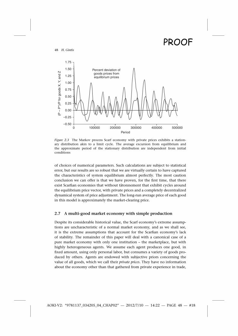
Figure 2.3. It is clear that by the time quasi-public prices have become estab-lished, the Markov process has attained its stationary distribution, which isa cycle around the equilibrium. This is the only behavior of the stationarydistribution observed, independent of the initial state of the system, so it isthe stationary distribution version of a limit cycle. In all observed cases, thestationary distribution has approximately the same period and amplitude.In sum, we have developed a dynamic mathematical model of Scarfian

exchange in the form of a Markov process. The transition probabilities of theMarkov process are specified implicitly by the algorithms for agent pairing, trad-ing, updating and reproduction. Except for the trade algorithm, for which alter-native algorithms are plausible, all modeling choices are uniquely determinedby the standard conception of the Walrasian general equilibrium model.The equilibrium of the Markov process is a stationary distribution that can

be analytically specified in principle, but in practice is orders of magnitude toolarge to calculate, even with the fastest and most powerful conceivable com-putational aids. Thus, as in the natural sciences, we are obliged to investigatethe stationary distribution by running the process on a computer with a variety

PROOF

AOKI-V2: “9781137_034205_04_CHAP02” — 2012/7/10 — 14:22 — PAGE 48 — #18

48 H. Gintis

0

1.75

1.50

1.25

1.00

0.75

0.50

0.25

(P –

P*)

/P fo

r go

ods

X, Y

, and

Z

–0.25

–0.50

0.00

100000 200000 300000Period

Percent deviation ofgoods prices fromequilibrium prices

400000 500000

Figure 2.3 The Markov process Scarf economy with private prices exhibits a station-ary distribution akin to a limit cycle. The average excursion from equilibrium andthe approximate period of the stationary distribution are independent from initialconditions

of choices of numerical parameters. Such calculations are subject to statisticalerror, but our results are so robust that we are virtually certain to have capturedthe characteristics of system equilibrium almost perfectly. The most cautionconclusion we can offer is that we have proven, for the first time, that thereexist Scarfian economies that without tâtonnement that exhibit cycles aroundthe equilibrium price vector, with private prices and a completely decentralizeddynamical system of price adjustment. The long-run average price of each goodin this model is approximately the market-clearing price.

2.7 A multi-good market economy with simple production

Despite its considerable historical value, the Scarf economy’s extreme assump-tions are uncharacteristic of a normal market economy, and as we shall see,it is the extreme assumptions that account for the Scarfian economy’s lackof stability. The remainder of this paper will deal with a canonical case of apure market economy with only one institution – the marketplace, but withhighly heterogeneous agents. We assume each agent produces one good, infixed amount, using only personal labor, but consumes a variety of goods pro-duced by others. Agents are endowed with subjective priors concerning thevalue of all goods, which we call their private prices. They have no informationabout the economy other than that gathered from private experience in trade,

PROOF

AOKI-V2: “9781137_034205_04_CHAP02” — 2012/7/10 — 14:22 — PAGE 49 — #19


including periodically discovering the private price vector of another agent theyhave encountered and copying it, with some possible mutation, if that agentappears to be more successful than himself. The only serious design decision isthat of the trade algorithm which, while much more straightforward than inthe case of the Scarf economy, is still in principle somewhat underspecified bythe logic of Walrasian exchange. Happily, the details of the trade protocol donot affect the dynamical movement to Walrasian equilibrium as far as we canascertain.We assume there are n sectors. Sector k = 1, . . .,n produces good k in ‘styles’

s = 1, . . .,m (we use ‘styles’ to enrich the heterogeneity of goods in the modelwithout seriously increasing the computational resources needed to estimatethe stationary distribution of the resulting Markov process). Each agent con-sumes a subset of non-production goods, but only a single style of any good.In effect, then, there are nm distinct goods gks , but only n production processesand correspondingly n equilibrium prices, since goods gks and gkt with styles sand t respectively, have the same production costs and hence the same price inequilibrium. We write the set of goods as G= {gks |k= 1, . . .,n,s= 1, . . .m}. We alsowrite g = gk when g = gks for some style s.A producer of good gks , termed a gks -agent, produces with no inputs other than

personal labor an amount qk of good gks which depreciates to zero at the end of atrading period. In a non-monetary economy, only the production good is carriedin inventory, but when individuals are permitted to acquire non-consumptiongoods, as in later sections of the paper, a trade inventory includes all goods thatare not the agent’s consumption goods.The Markov process is initialized by creating N agents, each of whom is

randomly assigned a production good gks . Thus, in an economy with goodsin m styles, there are Nnm traders. Each of these traders is assigned a privateprice vector by choosing each price from a uniform distribution on (0,1), thennormalizing so that the price of the nth good is unity. Each gks -agent is thenrandomly assigned a set H ⊆ G, gks /∈ H of consumption at most one style of agiven good.The utility function of each agent is the product of powers of CES utility func-

tions of the following form. Suppose an agent consumes r goods. We partitionthe r goods into k segments (k is chosen randomly from 1. . .r/2) of randomlychosen sizesm1, . . .,mk,mj >1 for all j, and

∑j mj =n. We randomly assign goods

to the various segments, and for each segment, we generate a CES consumptionwith random weights and an elasticity randomly drawn from the uniform dis-tribution on an interval [ε∗, ε∗]. Total utility is the product of the k CES utilityfunctions to random powers fj such that

∑j fj = 1. In effect, no two agent have

the same utility function.For example, consider a segment using goods x1, . . .,xm with prices p1, . . .,pm

and (constant) elasticity of substitution s, and suppose the power of this segment

PROOF

AOKI-V2: “9781137_034205_04_CHAP02” — 2012/7/10 — 14:22 — PAGE 50 — #20

50 H. Gintis

in the overall utility function is f . It is straightforward to show that the agentspends a fraction f of his income M on goods in this segment, whatever priceshe faces. The utility function associated with this segment is then

u(x1, . . .,xn) = m∑l=1

αlxγ

l

1/γ

, (32)

where γ = (s−1)/s, and α1, . . .,αm > 0 satisfy∑l αl = 1. The income constraint is∑m

l=1 plxl = fiM . Solving the resulting first-order conditions for utility maximiza-tion, and assuming γ �=0 (i.e., the utility function segment is notCobb-Douglas),this gives

xi = Mfi∑ml=1 plφ

1/(1−γ )

il

, (33)

where

φil = piαlplαifor i, l= 1, . . .,m.

When γ = 0 (which occurs with almost zero probability), we have a Cobb-Douglas utility function with exponents αl, so the solution becomes

xi = Mfiαipi. (34)

By creating such a complex array of utility functions, we ensure that ourresults are not the result of assuming an excessively narrow set of consumercharacteristics. However, the high degree of randomness involved in creatinga large number of agents ensures that all goods will have approximately thesame aggregate demand characteristics. If we add to this that all goods have thesame supply characteristics, we can conclude that themarket-clearingWalrasianequilibrium will occur when all prices are equal. This in fact turns out to bethe case. If we assume heterogeneous production conditions, then we cannotcalculate equilibrium prices, but we can still judge that the dynamical systemis asymptotically stable by the long-run standard error of the absolute value ofexcess demand, which will be very small in equilibrium.For each good gks ∈ G there is a market m[k,s] of traders who sell good gks . In

each period, the traders in the economy are randomly ordered and are permit-ted one by one to engage in active trading. When the ght -agent A is the currentactive trader, for each good ght for which A has positive demand (i.e, xA∗

h > 0), Ais assigned a random member B ∈m[h, t] who consumes gks . A then offers B themaximum quantity yk of gks , subject to the constraints yk ≤ iAk , where i

Ak repre-

sents A’s current inventory of good gks , and yk ≤ pAhxAh /pAk , where xAh is A’s current

demand for ght . This means that if A’s offer is accepted, A will receive in valueat least as much as he gives up, according to A’s private prices. A then offers

PROOF

AOKI-V2: “9781137_034205_04_CHAP02” — 2012/7/10 — 14:22 — PAGE 51 — #21


to exchange yk for an amount yh = pAk yk/pAh of good ght ; that is, he offers B anequivalent value of good ght , the valuation being at A’s prices. B accepts this offerprovided the exchange is weakly profitable at B’s private prices; that is, providedpBk yk ≥ pBhyh. However, B adjusts the amount of each good traded downward ifnecessary, while preserving their ratio, to ensure that what he receives does notexceed his demand, and what he gives is compatible with his inventory of ght . IfA fails to trade with this agent, he still might secure a trade giving him gks ,because A ∈ m[k,s] may also be on the receiving-end of trade offers fromght -agents at some point during the period. If a gks -agent exhausts his supplyof gks , he leaves the market for the remainder of the period.The assumption that each trading encounter is between agents each of whom

produces a good that the other consumes could be replaced by the assumptionis that each gks -producer A can locate the producers of his consumption goods,but that finding such a producer who also consumes gks will require a separatesearch. We simply collapse these two stages, noting that when a second searchis required and its outcome costly or subject to failure, the relative inefficiencyof the non-monetary economy, by comparison with the monetary economiesdescribed below, is magnified. Note, however, that while A’s partner is a con-sumer of gks , he may have fulfilled his demand for gks for this period by the timeA makes his offer, in which case no trade will take place.The trade algorithm involves only one substantive design choice, that of

allowing A to make a single ‘take-it-or-leave-it’ relative price offer, while oblig-ing A to accept quantity terms that are set by B, when it is feasible to do so. Suchalternatives as allowing B to make the take-it-or-leave-it offer, and choosing themean of the two offers provided that each is acceptable to the other, or using aNash bargaining solution, do not alter the market dynamics.After each trading period, agents consume their inventories provided they

have a positive amount of each good that they consume, and agents replen-ish the amount of their production good in inventory. Moreover, each traderupdates his private price vector on the basis of his trading experience over theperiod, raising the price of a consumption or production good by 0.05 per centif his inventory is empty (that is, if he failed to purchase any of the consump-tion good or sell all of his production good), and lowering price by 0.05 percent otherwise (that is, if he succeeded in obtaining his consumption good orsold all his production inventory). We allow this adjustment strategy to evolveendogenously according to an imitation processes.After a number of trading periods, the population of traders is updated using

the following process. For each market m[k,s] and for each gks -trader A, let fA

be the accumulated utility of agent A since the last updating period (or sincethe most recent initialization of the Markov process if this is the first updatingperiod). Let f∗ and f ∗ be the minimum and maximum, respectively, over f A

for all gks -agents A. For each gks -agent A, let p

A = (f A − f∗)/(f ∗ − f∗), so pA is a

PROOF

AOKI-V2: “9781137_034205_04_CHAP02” — 2012/7/10 — 14:22 — PAGE 52 — #22

52 H. Gintis

probability for each A. If r agents are to be updated, we repeat the followingprocess by r times. First, choose an agent for reproducing as follows. Identify arandom agent inm[k,s] and choose this agent for reproduction with probabilitypA. If A is not chosen, repeat the process until one agent is eventually chosen.Note that a relatively successful trader is more likely to be chosen to reproducethan an unsuccessful trader. Next, choose an agent B to copy A’s private prices asfollows. Identify a random agent B in m[k,s] and choose this agent with proba-bility 1−pB. If B is not chosen, this process is repeated until B is chosen. Clearly,a less successful trader is likely to be chosen this criterion. Repeat until an agentB is chosen. Finally, endow B with A’s private price vector, except for each suchprice, with a small probability µ = randomly increase or decrease its value bya small percentage ∈. The resulting updating process is a discrete approxima-tion of a monotonic dynamic in evolutionary game theory, and in differentialequation systems, all monotonic dynamics have the same dynamical proper-ties (Taylor and Jonker, 1978; Samuelson and Zhang, 1992). Other monotonicapproximations, including the simplest, which is repeatedly to choose a pair ofagents in m[k,s] and let the lower-scoring agent copy the higher-scoring agent,produce similar dynamical results.Using utility as the imitation criterion is quite noisy, because utility functions

are heterogeneous and individuals who prefer goods with low prices do betterthan agents who prefer high-priced goods independent of the trading prowess.Using alternative criteria, such as the frequency and/or volume trading success,with results similar to those reported herein.The result of the dynamic specified by the above conditions is the change over

time in the distribution of private prices. The general result is that the systemof private prices, which at the outset are randomly generated, in rather shorttime evolves to a set of quasi-public prices with very low inter-agent variance.Over the long term, these quasi-public prices move toward their equilibrium,market-clearing levels.

2.8 Estimating the stationary distribution

I will illustrate this dynamic assuming n= 9,m= 6, and N = 300, so there are 54distinct goods which we write as g11 , . . .,g

96 , and 16,200 traders in the economy.

There are then nine distinct prices pA1 , . . .,pA9 for each agent A. We treat g9 as the

numeraire good for each trader, so pA9 = 1 for all traders A. A gk-agent producesone unit of good k per period. We assume that there are equal numbers ofproducers of each good from the outset, although we allow migration from lessprofitable to more profitable sectors, so in the long run profit rates are closeto equal in all sectors. The complexity of the utility functions do not allow usto calculate equilibrium properties of the system perfectly, but we will assumethat market-clearing prices are approximately equal to unit costs, given that

PROOF

AOKI-V2: “9781137_034205_04_CHAP02” — 2012/7/10 — 14:22 — PAGE 53 — #23


unit costs are fixed, agents can migrate from less to more profitable sectors,and utility functions do not favor one good or style over another, on average.Population updating occurs every ten periods, and the number of encountersper sector is 10 per cent of the number of agents in the sector. The mutationrate is µ = 0.01 and the error correction is ∈= 0.01.The results of a typical run of this model are illustrated in Figures 2.4 to 2.6.

Figure 2.4 shows the passage from private to quasi-public prices over the first20,000 trading periods of a typical run. The mean standard error of prices iscomputed as follows. For each good g we measure the standard deviation of theprice of g across all g-agents, where for each agent, the price of the numerairegood g9 is unity. Figure 2.4 shows the average of the standard errors for all goods.The passage from private to quasi-public prices is quite dramatic, the standarderror of prices across individuals falling by an order of magnitude within 300periods, and falling another order of magnitude over the next 8,500 periods.The final value of this standard error is 0.029, as compared with its initial valueof 6.7.Figure 2.5 shows the movement of the average standard error of the absolute

value of excess demand over 50,000 periods for nine goods in six styles each.Using this measure, after 1,500 periods excess demand has decreased by twoorders of magnitude, and it decreases another order of magnitude by the end ofthe run.It is not surprising, given the behavior of excess demand for this model,

that prices would approach their Walrasian equilibrium values. This process

Convergence from privateto quasi-public prices

fifty four goods

0

00.51.0

Sta

ndar

d er

ror

of p

rices

acr

oss

trad

ers

1.52.02.53.03.54.04.55.05.56.06.57.0

250 500 750 1000

Periods

1250 1500 1750 2000 20000

Figure 2.4 Convergence of private prices to quasi-public prices in a typical run with ninegoods in 6 sytles each (fifty-four goods)

PROOF

AOKI-V2: “9781137_034205_04_CHAP02” — 2012/7/10 — 14:22 — PAGE 54 — #24

54 H. Gintis

Passage to Walrasian Quasi-Equilibrium:Average absolute excess demand

fifty-four goods, 100-periodrunning average

0

2

4

6

8

10

12

14

40A

vera

ge a

bsol

ute

exce

ss d

eman

d

0 250 500 750 1000

Periods

1250 1500 50000

Figure 2.5 The path of aggregate excess demand over 50,000 periods

0

Ave

rage

sta

ndar

d er

ror

of (

P –

P*)

/P*

0.00

0.05

0.10

0.15

0.20

0.25

0.30

0.35

0.40

0.45

0.50

1.00

2000 4000 6000 8000

Periods

10000 12000 14000 50000

Passage to Walrasian Quasi-Equilibrium:Average standard error of deviation

of Quasi-Public Price fromWalrasian Equilibrium Price

fifty-four goods

Figure 2.6 The passage from private to quasi-public prices in the Markovian Scarf econ-omy. The long-run standard error of prices across traders is rather high, due to the factthat the system does not tend to Walrasian equilibrium

is illustrated in Figure 2.6. After 50,000 periods, the standard error of the devi-ation of prices from (our calculated) equilibrium values are about 3 per cent ofits starting value.

PROOF

AOKI-V2: “9781137_034205_04_CHAP02” — 2012/7/10 — 14:22 — PAGE 55 — #25


The distinction between low-variance private prices and true public pricesis significant, even when the standard error of prices across agents is extremelysmall, because stochastic events such as technical changes propagate very slowlywhen prices are highly correlated private prices, but very rapidly when all agentsreact in parallel to price movement. In effect, with private prices, a large partof the reaction to a shock is a temporary reduction in the correlation amongprices, a reaction that is impossible with public prices, as the latter are alwaysperfectly correlated.There is nothing special about the parameters used in the above example. Of

course, adding more goods or styles increases the length of time until quasi-public prices become established, as well as the length of time until marketquasi-equilibrium is attained. Increasing the number of agents increases thelength of both of these time intervals.

2.9 The emergence of money

There is no role for money in the Walrasian general equilibrium model becauseall adjustments of ownership are carried out simultaneously when the equi-librium prices are finally set. When there is actual exchange among individualagents in an economy, twomajor conditions give rise to the demand for money,by which we mean a good that is accepted in exchange not for consumption orproduction, but rather for resale at a later date against other intrinsically desiredgoods. The first is the failure of the ‘double coincidence of wants’ (Jevons, 1875),explored in recent years in this and other journals by Starr (1972) and Kiyotakiand Wright (1989, 1991, 1993). The second condition is the existence of trans-actions costs in exchange, the money good is likely to be that which has thelowest transactions cost (Foley, 1970; Hahn, 1971, 1973; Kurz, 1974b, 1974a;Ostroy, 1973; Ostroy and Starr, 1974; Starrett, 1974). We show that these con-ditions interact in giving rise to a monetary economy. When one traded goodhas very low transactions costs relative to other goods, this good may come tobe widely accepted in trade even by agents who do not consume or produce it.Moreover, when an article that is neither produced nor consumed can be tradedwith very low transactions costs, this good, so-called fiat money. will emerge asa universal medium of exchange.We now permit traders to buy and sell at will any good that they neither

consumer nor produce. We call such a good a money good, and if there is ahigh frequency of trade in one or more money goods, we say the market econ-omy is a money economy. We assume that traders accept all styles of a moneygood indifferently. We first investigate the emergence of money from marketexchange by assuming zero inventory costs, so the sole value of money is tofacilitate trade between agents, even though the direct exchange of consump-tion and production goods between a pair of agents might fail because one of

PROOF

AOKI-V2: “9781137_034205_04_CHAP02” — 2012/7/10 — 14:22 — PAGE 56 — #26

56 H. Gintis

the parties is not currently interested in buying the other’s production good.The trade algorithm in case agents accept a good that they do not consume isas follows. At the beginning of each period, each agent calculates how much ofeach consumption good he wants to acquire during that period, as follows. Theagent calculates the market value of his inventory of production and moneygoods he holds in inventory, valued at his private prices. This total is the agent’sincome constraint. The agent then chooses an amount of each consumptiongood to purchase by maximizing utility subject to this income constraint. Thetrade algorithm is similar to the case of the pure market, except that either partyto a trade may choose to offer and/or accept a money good in the place of hisproduction good.We evaluate the performance of this economy using the same parameters as

in our previous model, including zero inventory costs. Figure 2.7 shows thatthe use of money increases monotonically over the first 2,000 periods, spreadalmost equally among the remaining goods. From period 2,000 to period 4,000,one good becomes a virtually universal currency, driving the use of the othersto low levels. It is purely random which good becomes the universal medium ofexchange, but one does invariable emerge as such after several thousand periods.If we add inventory costs with g1 being lower cost than the others, g1 invariablyemerges as the medium of exchange after 1,000 periods, and the other goods arenot used as money at all. I did not include graphs of the passage to quasi-publicprices or other aspects of market dynamics because they differ little from thebaseline economy described above.

Period

Other goods

The frequency with whichvarious goods are

accepted as money.Zero inventory costs

Good 3

00.0

0.1

0.2

0.3

0.4

0.5

Freq

uenc

y ac

cept

as

mon

ey

0.6

0.7

0.8

0.9

1.0

2000 4000 6000 8000 10000

Figure 2.7 The emergence of money in a market economy. The parameters of the modelare the same as in the baseline case treated previously. inventory costs are assumeabsent

PROOF

AOKI-V2: “9781137_034205_04_CHAP02” — 2012/7/10 — 14:22 — PAGE 57 — #27


Number of goods and styles

200 0.0

0.1

0.2

0.3

0.4

0.5

0.6

0.7

0.8

1

2

Rel

ativ

e ef

ficie

ncy

of m

oney

ove

r no

n-m

oney

3

Relative efficiency ofmoney over non-money

(left axis)

Absolute efficiencyof money trade

(right axis)

Absolute efficiencyof non-money trade

(right axis)

Abs

olut

e ef

ficie

ncy

of m

oney

and

non

-mon

ey tr

ade

4

5

6

7

8

9

10

11

12

40 60 80 100 120 140 160 180

Figure 2.8 The relative efficiency of money in a market economy

As in traditional monetary theory (Menger, 1892; Wicksell, 1911; Kiyotakiand Wright, 1989, 1991) money emerges from goods trade both because it isa low transactions cost good and it solves the problem of the ‘double coinci-dence of wants’ that is required for market exchange (Jevons, 1875). The relativeefficiency of money over direct goods trade increases with the number of goods,as illustrated in Figure 2.8. While with six goods and one style the relative effi-ciency of money is only 150 per cent, for nine goods and twenty styles (180goods), the relative efficiency is 1,200 per cent.

2.10 The resilience of the decentralized market economy

We now show that the above Markov model is extremely resilient in the face ofaggregate shocks when the number of producers per good is sufficiently large,but becomes unstable when this number falls below a certain (relatively high)threshold. We illustrate this in the context of a fiat money economy. We takethe non-monetary economy described above, with nine goods in six styles each,and add a single new good that is neither produced nor consumed, and haszero inventory storage costs. When such a good is available, it quickly becomesa universal medium of exchange for the economy, accepted by almost 100 percent of market traders. The nature of market dynamics in a fiat money economyis not noticeably different from the economies described above.In this fiat money economywith 300 producers per good, every 1,000 periods,

we impose an aggregate shock on the economy consisting of a reduction in thefiat money holdings of each trader to 20 per cent of its normal level, as shown in

PROOF

AOKI-V2: “9781137_034205_04_CHAP02” — 2012/7/10 — 14:22 — PAGE 58 — #28

58 H. Gintis

Period

Flat money per trader

00

20

40

Sup

ply

of m

oney

60

80

100

120

10000 20000 30000 40000 50000

Figure 2.9 To test the resilience of the Markov economy, we impose a periodicshock, sustained for 100 periods, that reduces the money supply to 20% of itsnormal level

Period0

0.0

0.5

Frac

tion

devi

atio

n

1.0

3.0

Deviation of goods prices fromequilibrium and standard deviation

of prices across tradersnine goods, three hundred

producers per good

20000 40000 60000 80000 100000

Figure 2.10 Walrasian equilibrium is reilient to aggregate shocks. With 300 producers pergood, we impose an aggregate shock on the Markov process consisting of halving themoney supply every 1000 periods, and restoring the money supply after 100 periods haveelapsed with the smaller money supply. There is virtually no effect on the passage to aquasi-Walrasian equilibrium

Figure 2.9. The reduced holding are maintained for 100 periods, after which themoney holdings of each trader is multiplied by two, restoring the money stockfor the economy to its initial level. Figure 2.10 shows the effect of the periodshock on average prices and on the standard error of prices across traders; there

PROOF

AOKI-V2: “9781137_034205_04_CHAP02” — 2012/7/10 — 14:22 — PAGE 59 — #29


Period0 20000 40000

Average standard deviation ofabsolute value of excess supply

nine goods, 300 producers per good

0.00

0.05

0.10Exc

ess

supp

ly

0.15

0.20

0.25

1.40

60000 80000 100000

Figure 2.11 Excess demand is resilient in the face of large macro-level shocks. The param-eters are as in the previous figure. Note that there is virtually no effect on aggregate excessdemand in any sector of the economy

is no noticeable effect. Figure 2.11 shows that the quantity side of the economyis also virtually unaffected by the system of aggregate shocks.

2.11 Conclusion

The search for stability of market exchange using differential equations withpublic prices, while producing some brilliantmathematical analyses, was doublydefective. First, no plausible dynamic price and quantity adjustment mecha-nism was found. Second, such a dynamic, even were it found, would be ofdoubtful value because out of equilibrium public prices cannot exist in a decen-tralized market economy. By modeling market exchange as a Markov process,we have shown that under plausible conditions we get convergence to a quasi-equilibrium. However, under the extreme conditions of the Scarf economy (onlythree goods, three traders, and fixed coefficients utility functions) we get astationary distribution akin to a limit cycle in continuous models. With a plain-vanilla Walrasian economy with individual production, we find global stabilityunder a wide range of parameters. Yet we do not have the analytical machin-ery to ascertain when Scarf instability will hold, when global stability holds, orwhether there are other possible dynamic characteristics of a Markovian marketsystem.On the positive side, we have proved that certain Markov models of market

dynamics are globally stable over a wide range of parameters. This is an existencetheorem possibly as informative as the existence proofs for general equilibrium.Computational proofs, however, are not as powerful as purely analytical proofs.

PROOF

AOKI-V2: “9781137_034205_04_CHAP02” — 2012/7/10 — 14:22 — PAGE 60 — #30

60 H. Gintis

Those unused to working with complex dynamical systems may object thata computational proof is no proof at all. In fact, a computational proof maynot be a mathematical proof, but it is a scientific proof: it is evidential ratherthan tautological, and depends on induction rather than deduction. The naturalsciences, in which complex systems abound, routinely use mathematical tomodels that admit no closed-form analytical solutions, ascertain their propertiesthrough approximation and simulation, and justify these models by virtue ofhow they conform empirical reality. This appears to be the current state of affairswith respect to Markov processes and general equilibrium theory.

References

Arrow, Kenneth and Leonid Hurwicz (1958) ‘On the Stability of the CompetitiveEquilibrium, I’, Econometrica, vol. 26, pp. 522–552.

Arrow, Kenneth and Leonid Hurwicz (1959) ‘Competitive Stability UnderWeak Gross Sub-stitutability: Nonlinear Price Adjustment and Adaptive Expectations’, Technical Report,Office of Naval Research Contract Nonr-255, Department of Economics, StanfordUniversity, Technical Report No. 78.

Arrow, Kenneth and LeonidHurwicz (1960) ‘Some Remarks on the Equilibria of EconomicsSystems’, Econometrica, vol. 28, pp. 640–646.

Arrow, Kenneth, H.D. Block and Leonid Hurwicz (1959) ‘On the Stability of theCompetitive Equilibrium, II’, Econometrica, vol. 27, pp. 82–109.

Arrow, Kenneth J. ‘An Extension of the Basic Theorems of Classical Welfare Economics’, inJ. Neyman (ed.), Proceedings of the Second Berkeley Symposium on Mathematical Statisticsand Probability (Berkeley: University of California Press, 1951), pp. 507–532.

Arrow, Kenneth J. andGérardDebreu (1954) ‘Existence of an Equilibrium for aCompetitiveEconomy’, Econometrica, vol. 22,no. 3, pp. 265–290.

Aumann, Robert J. and Adam Brandenburger (1995) ‘Epistemic Conditions for NashEquilibrium’, Econometrica, vol. 65, no. 5, pp. 1161–1180.

Bala, V. and M. Majumdar (1992) ‘Chaotic Tâtonnement’, Economic Theory, vol. 2, pp.437–445.

Debreu, Gérard (1951) ‘The Coefficient of Resource Utilization’, Econometrica, vol. 19,273–292.

Debreu, Gérard (1952) ‘A Social Equilibrium Existence Theorem’, Proceedings of the NationalAcademy of Sciences, vol. 38, pp. 886–893.

Debreu, Gérard (1954) ‘Valuation Equilibrium and Pareto Optimum’, Proceedings of theNational Academy of Sciences, vol. 40, pp. 588–592.

Debreu, Gérard (1974) ‘Excess Demand Function’, Journal of Mathematical Economics, vol.1, pp. 15–23.

Feller, William (1950) An Introduction to Probability Theory and Its Applications, vol. 1 (NewYork: John Wiley & Sons).

Fisher, Franklin M. (1983)Disequilibrium Foundations of Equilibrium Economics (Cambridge:Cambridge University Press).

Fisher, Franklin M. (1999) Microeconomics: Essays in Theory and Applications, ed. MaartenPieter Schinkl (Cambridge, UK: Cambridge University Press).

Foley, Duncan (1970) ‘Economic Equilibria with Costly Marketing’, Journal of EconomicTheory, vol. 2, pp. 276–291.

PROOF

AOKI-V2: “9781137_034205_04_CHAP02” — 2012/7/10 — 14:22 — PAGE 61 — #31


Gale, David (1955) ‘The Law of Supply and Demand’, Math. Scand., vol. 30, pp. 155–169.Gintis, Herbert (2007) ‘The Dynamics of General Equilibrium’, Economic Journal, vol. 117,

pp. 1289–1309.Gintis, Herbert (2009) Game Theory Evolving, second edition (Princeton, NJ: Princeton

University Press).Hahn, Frank (1962) ‘A Stable Adjustment Process for a Competitive Economy’, Review ofEconomic Studies, vol. 29, pp. 62–65.

Hahn, Frank (1971) ‘Equilibrium with Transactions Costs’, Econometrica, vol. 39, pp. 417–439.

Hahn, Frank (1973) ‘On Transactions Costs, Inessential Sequence Economies and Money’,Review of Economic Studies, vol. 40, pp. 449–461.

Hahn, Frank and Takashi Negishi (1962) ‘A Theorem on Non- tâtonnement Stability’,Econometrica, vol. 30, pp. 463–469.

Hayek, F.A. (1945) ‘The Use of Knowledge in Society’, American Economic Review, vol. 35,no. 4, pp. 519–530.

Hofbauer, Josef and Karl Sigmund (1998) Evolutionary Games and Population Dynamics(Cambridge: Cambridge University Press).

Howitt, Peter and Robert Clower (2000) ‘The Emergence of Economic Organization’,Journal of Economic Behavior and Organization, vol. 41, pp. 55–84.

Hurwicz, Leonid (1960) ‘Optimality and Informational Efficiency in Resource AllocationProcesses’, inMathematical Methods in Social Sciences (Stanford, CA: Stanford UniversityPress), pp. 27–46.

Jevons, William Stanley (1975) Money and the Mechanism of Exchange (London: D.Appleton Co.).

Kirman, Alan P. (1992) ‘Whom or What does the Representative Individual Represent?’,Journal of Economic Perspectives, vol. 6, pp. 117-136.

Kiyotaki, Nobuhiro and Randall Wright (1989) ‘On Money as a Medium of Exchange’,Journal of Political Economy, vol. 94, no. 4, 927–954.

Kiyotaki, Nobuhiro and Randall Wright (1991) ‘A Contribution to a Pure Theory ofMoney’, Journal of Economic Theory, vol. 53, no. 2, 215–235.

Kiyotaki, Nobuhiro and Randall Wright (1993) ‘A Search-Theoretic Approach to MonetaryEconomics’, American Economic Review, vol. 83, no. 1, pp. 63–77.

Kurz, Mordecai (1974a) ‘Equilibrium in a Finite Sequence of Markets with TransactionsCosts’, Econometrica, vol. 42, pp. 1–20.

Kurz, Mordecai (1974b) ‘Equilibrium with Transactions Cost and Money in a SingleMarket’, Journal of Economic Theory, vol. 7 pp. 418–452.

Mantel, Rolf (1974) ‘On the Characterization of Aggregate Excess Demand’, Journal ofEconomic Theory, vol. 7, pp. 348–353.

Mantel, Rolf (1976) ‘Homothetic Preferences and Community Excess Demand Functions’,Journal of Economic Theory, vol. 12, pp. 197–201.

McKenzie, L.W. (1959) ‘On the Existence of a General Equilibrium for a CompetitiveMarket’, Econometrica, vol. 28, pp. 54–71.

McKenzie, L.W. (1960) ‘Stability of Equilibrium and Value of Positive Excess Demand’,Econometrica 28 (1960): 606–617.

Menger, Karl (1982) ‘On the Origin of Money’, Economic Journal, vol. 2, pp. 239–255.Morishima, Michio (1960) ‘A Reconsideration of the Walras–Cassel–Leontief Model of

General Equilibrium’, inMathematical Methods in Social Sciences (Stanford, CA: StanfordUniversity Press), pp. 63–76.

PROOF

AOKI-V2: “9781137_034205_04_CHAP02” — 2012/7/10 — 14:22 — PAGE 62 — #32

62 H. Gintis

Negishi, Takashi (1960) ‘Welfare Economics and the Existence of an Equilibrium for aCompetitive Economy’, Metroeconomica, vol. 12, pp. 92–97.

Negishi, Takashi (1961) ‘On the Formation of Prices’, International Economic Review, vol. 2,pp. 122–126.

Nikaido, Hukukaine (1956) ‘On the Classical Multilateral Exchange Problem’, MetroEco-nomica, vol. 8, 135–145.

Nikaido, Hukukaine (1959) ‘Stability of Equilibrium by the Brown–von Neumann Differ-ential Equation’, MetroEconomica 27 (1959): 645–671.

Nikaido, Hukukaine and Hirofumi Uzawa (1960) ‘Stability and Nonnegativity in aWalrasian Tâtonnement Process’, International Economic Review, vol. 1, pp. 50–59.

Ostroy, Joseph (1973) ‘The Informational Efficiency of Monetary Exchange’, AmericanEconomic Review, vol. 63, 597–610.

Ostroy, Joseph and Ross Starr (1974) ‘Money and the Decentralization of Exchange’,Econometrica, vol. 42, pp. 1093–1113.

Saari, Donald G. (1985) ‘Iterative PriceMechanisms’, Econometrica, vol. 53, pp. 1117–1131.Saari, Donald G. (1995) ‘Mathematical Complexity of Simple Economics’, Notices of theAmerican Mathematical Society, vol. 42, no. 2, pp. 222–230.

Samuelson, Larry and Jianbo Zhang (1992) ‘Evolutionary Stability in Asymmetric Games’,Journal of Economic Theory, vol. 57, no. 2 pp. 363–391.

Scarf, Herbert (1960) ‘Some Examples of Global Instability of Competitive Equilibrium’,International Economic Review, vol. 1, pp. 157–172.

Smith, Adam (2000 [1759]) The Theory of Moral Sentiments (New York: Prometheus).Sonnenschein, Hugo (1973) ‘Do Walras’ Identity and Continuity Characterizethe Class of

Community Excess Demand Functions?’, Journal of Ecomonic Theory, vol. 6, pp. 345–354.

Starr, Ross (1972) ‘The Structure of Exchange in Barter andMonetary Economies’, QuarterlyJournal of Economics, vol. 86, no. 2, pp. 290–302.

Starrett, David (1974) ‘Inefficiency and the Demand for “Money” in a Sequence Economy’,Review of Economic Studies, vol. 40, pp. 437–448.

Taylor, Peter and Leo Jonker (1978) ‘Evolutionarily Stable Strategies and Game Dynamics’,Mathematical Biosciences, vol. 40, pp. 145–156.

Uzawa, Hirofumi (1959) ‘Edgeworth’s Barter Process and Walras’ Tâtonnement Process’,Technical Report, Office of Naval Research Contract NR-047-004, Department ofEconomics, Stanford University. Technical Report No. 83.

Uzawa, Hirofumi (1961) ‘The Stability of Dynamic Processes’, Econometrica, vol. 29, no. 4,617–631.

Uzawa, Hirofumi (1962) ‘On the Stability of Edgeworth’s Barter Process’, InternationalEconomic Review, vol. 3, no. 2, pp. 218–231.

Wald, Abraham (1951 [1936]) ‘On Some Systems of Equations of Mathematical Eco-nomics’, Econometrica, vol. 19, no. 4, pp. 368–403.

Walras, Leon (1954 [1874]) Elements of Pure Economics (London: George Allen and Unwin).Wicksell, Knut (1967 [1911]) Lectures in Political Economy, Vol. 2. Money (New York: Kelley).

PROOF

part ii complex economic dynamics: agent-based and analytical

Documents