part ii: interpolation and approximation theorydmackey/lectures/interpolationii.pdf · polynomial...

Part II: Interpolation and Approximation theory

Contents:

1 Review of Lagrange interpolation polynomials

2 Newton interpolation

3 Optimal interpolation points; Chebyshev polynomials

4 Cubic spline interpolation

5 Error analysis

Numerical Methods January 29, 2016 1 / 47

Interpolation is the process of finding a function f (x) whose graph passesthrough a given set of data points (x0, y0), (x1, y1), ... (xn, yn). In otherwords, we know the values of the function at n+ 1 points:

f (x0) = y0, f (x1) = y1 . . . f (xn) = yn

and we need to find an analytic expression for f (x), which would thenspecify the values of the function at other points, not listed among the xi ’s.

In interpolation, we need to estimate f (x) for arbitrary x that lies betweenthe smallest and the largest xi . (If x is outside the range of the xi s, thisis called extrapolation.)


Polynomial interpolation

The most common functions used for interpolation are polynomials.

Given a set of n + 1 data points (xi , yi ) , we want to find a polynomialcurve that passes through all the points.

A polynomial P for which P(xi) = yi when 0 ≤ i ≤ n is said to interpolatethe given set of data points. The points xi are called nodes orinterpolating points.

For the simple case of n = 1, we have two points: (x0, y0) and (x1, y1).We can always find a linear polynomial, P1(x) = a0 + a1x , passing throughthe given points and show that it has the form

P1(x) =x − x1

x0 − x1y0 +

x − x0

x1 − x0y1 = L1,0(x) y0 + L1,1(x) y1.


The Lagrange form of the interpolating polynomialIf n + 1 data points, (x0, y0), . . . (xn, yn), are available, then we can find apolynomial of degree n, Pn(x), which interpolates the data, that is

Pn(xi ) = yi , 0 ≤ i ≤ n

The Lagrange form of the interpolating polynomial is

Pn(x) =n∑

i=0

Ln,i (x)yi ,

where

Ln,i (x) =

n∏

k=0k 6=i

x − xk

xi − xk

=(x − x1)(x − x2) · · · (x − xi−1)(x − xi+1) · · · (x − xn)

(xi − x1)(xi − x2) · · · (xi − xi−1)(xi − xi+1) · · · (xi − xn)


It has the property that

Ln,i (xj ) =

{1 i = j

0 i 6= j

Example: Consider the function f (x) = ln(x)

1 Construct the Lagrange form of the interpolating polynomial for f (x)which passes through the points (1, ln(1)), (2, ln(2)) and (3, ln(3)).

2 Use the polynomial in part (a) to estimate ln(1.5) and ln(2.4). Whatis the error in each approximation?


Graphical representation

Figure: The polynomial P2(x) which interpolates the points (1, ln(1)), (2, ln(2))and (3, ln(3)) (solid curve). The graph of ln(x) is shown as the dotted curve.


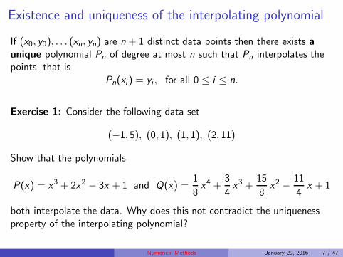
Existence and uniqueness of the interpolating polynomial

If (x0, y0), . . . (xn, yn) are n + 1 distinct data points then there exists aunique polynomial Pn of degree at most n such that Pn interpolates thepoints, that is

Pn(xi ) = yi , for all 0 ≤ i ≤ n.

Exercise 1: Consider the following data set

(−1, 5), (0, 1), (1, 1), (2, 11)

Show that the polynomials

P(x) = x3 + 2x2 − 3x + 1 and Q(x) =1

8x4 +

3

4x3 +

15

8x2 − 11

4x + 1

both interpolate the data. Why does this not contradict the uniquenessproperty of the interpolating polynomial?


The Newton interpolation polynomial

Consider a set of n+ 1 data points, (x0, y0), . . . (xn, yn), and assume theyare given by a function f , so that y0 = f (x0), . . . , yn = f (xn).

We introduce the following quantities, called divided differences:

f [xk ] = f (xk),

f [xk , xk+1] =f [xk+1]− f [xk ]

xk+1 − xk

f [xk , xk+1 xk+2] =f [xk+1, xk+2]− f [xk , xk+1]

xk+2 − xk

f [xk , xk+1 xk+2, xk+3] =f [xk+1, xk+2, xk+3]− f [xk , xk+1, xk+2]

xk+3 − xk...


Newton’s divided differences formula

The Newton form of the interpolation polynomial is given by the divideddifference formula:

Pn(x) = f [x0] + f [x0, x1] (x − x0) + f [x0, x1, x2] (x − x0)(x − x1)

+f [x0, x1, x2, x3] (x − x0)(x − x1)(x − x2) + · · ·+f [x0, x1 . . . xn] (x − x0)(x − x1) · · · (x − xn)

Exercise 2: Use both the Lagrange and Newton methods to find aninterpolating polynomial of degree 2 for the following data

(0, 1), (2, 2), (3, 4).

Check that both methods yield the same polynomial!


Derivation of the Newton formula

Look for an interpolating polynomial in the “nested” form

Pn(x) = a0 + a1(x − x0) + a2(x − x0)(x − x1) + · · ·+ an(x − x0) · · · (x − xn)

=

n∑

k=0

ak

[k−1∏

i=0

(x − xi)

]

Then the interpolating conditions yield

f (x0) = Pn(x0) = a0

f (x1) = Pn(x1) = a0 + a1(x1 − x0)

f (x2) = Pn(x2) = a0 + a1(x2 − x0) + a2(x2 − x0)(x2 − x1)

...


Exercise 3: Show that

a0 = f (x0) ≡ f [x0]

a1 =f (x1)− f (x0)

x1 − x0≡ f [x0, x1]

a2 =f [x1, x2]− f [x0, x1]

x2 − x0≡ f [x0, x1, x2]

Exercise 4: Suppose that, in addition to the three points considered inExercise 1, a new point becomes available so now we must construct aninterpolating polynomial for the data

(0, 1), (1, 3), (2, 2), (3, 4)

Construct the new polynomial using both the Lagrange and Newtonmethods. Which one is easier?


Lagrange Interpolation error

Let f be a continuous function on an interval [a, b], which has n + 1continuous derivatives.

If we take n+ 1 distinct points on the graph of the function, (xi , yi) for0 ≤ i ≤ n so that yi = f (xi), then the interpolating polynomial Pn(x)satisfies

f (x)− Pn(x) =f (n+1)(ξ)

(n + 1)!(x − x0)(x − x1) · · · (x − xn)

where ξ is a point between a and b.


Newton form of the interpolation error

If the polynomial Pn interpolates the data (x0, f (x0)), . . ., (xn, f (xn)) thenthe interpolation error can also be written as

f (x)− Pn(x) = f [x0, x1, . . . , xn, x ] (x − x0)(x − x1) · · · (x − xn)

Note that the errors given by the Lagrange and Newton forms above areequal.

Exercise 5: Construct the Lagrange and Newton forms of theinterpolating polynomial P3(x) for the function f (x) = 3

√x which passes

through the points (0,0), (1,1), (8,2) and (27,3). Calculate theinterpolation error at x = 5 and compare with the theoretical error bound.


Optimal points for interpolation

Assume that we need to approximate a continuous function f (x) on aninterval [a, b] using an interpolation polynomial of degree n and we havethe freedom to choose the interpolation nodes x0, x1, . . . , xn.

The optimal points will be chosen so that the total interpolation error is assmall as possible, which means that the worst case error,

maxa≤x≤b

|f (x)− Pn(x)|,

is minimized.

In what follows we show that the optimal points for interpolation are givenby the zeros of special polynomials called Chebyshev polynomials.


Chebyshev polynomials

For any integer n ≥ 0 define the function

Tn(x) = cos(n cos−1(x)), −1 ≤ x ≤ 1

We need to show that Tn(x) is a polynomial of degree n. We calculate thefunctions Tn(x) recursively.

Let θ = cos−1(x) so cos(θ) = x . Then

Tn(x) = cos(nθ)

Easy to see that:

n = 0 =⇒ T0(x) = cos(0) = 1

n = 1 =⇒ T1(x) = cos(θ) = x

n = 2 =⇒ T2(x) = cos(2θ) = 2 cos2(θ)− 1 = 2x2 − 1


Recurrence relations for Chebyshev polynomials

Using trigonometric formulas we can prove that

Tn+m(x) + Tn−m(x) = 2Tn(x)Tm(x)

for all n ≥ m ≥ 0 and all x ∈ [−1, 1].

Hence, for m = 1 we get

Tn+1(x) + Tn−1(x) = 2xTn(x)

which is then used to calculate the Chebyshev polynomials of higher order.

Example: Calculate T3(x), T4(x) and T5(x).


More properties of Chebyshev polynomials

Note that|Tn(x)| ≤ 1

andTn(x) = 2n−1xn + lower degree terms

for all n ≥ 0 and all x in [−1, 1].

If we define the modified Chebyshev polynomial:

T̃n(x) =Tn(x)

2n−1

then we have

|T̃n(x)| ≤1

2n−1and T̃n(x) = xn + lower degree terms

for all n ≥ 0 and all x in [−1, 1].


Zeros of Chebyshev polynomials

We haveTn(x) = cos(nθ), θ = cos−1(x)

so

Tn(x) = 0 =⇒ nθ = ±π

2, ±3π

2, ±5π

2, . . .

which implies

θ = ±(2k + 1)π

2n, k = 0, 1, 2, . . .

and hence the zeros of Tn(x) are given by

xk = cos

[(2k + 1)π

2n

], k = 0, 1, 2, . . . n − 1.


The minimum size property

Let n ≥ 1 be an integer and consider all possible monic polynomials (thatis, polynomials whose highest-degree term has coefficient equal to 1) ofdegree n.

Then the degree n monic polynomial with the smallest maximum absolutevalue on [−1, 1] is the modified Chebyshev polynomial T̃n(x) and itsmaximum value is 1/2n−1. In other words,

1

2n−1= max

−1≤x≤1|T̃n(x)| ≤ max

−1≤x≤1|Pn(x)|

for any monic polynomial of degree n, Pn(x).


Optimal interpolating points

Let f (x) be a continuous function on [−1, 1]. We are looking for anapproximation given by an interpolating polynomial of degree n, Pn(x).Let x0, x1, x2, . . . , xn be the interpolating nodes.

Recall the formula for the interpolation error:

f (x)− Pn(x) =(x − x0)(x − x1) · · · (x − xn)

(n + 1)!f (n+1)(ξ)

where ξ is in [−1, 1].

We need to find the interpolating points so that we minimize

E [Pn] = max−1≤x≤1

|f (x)− Pn(x)|


This is equivalent to minimizing

max−1≤x≤1

|(x − x0)(x − x1) · · · (x − xn)|

But we know that the minimum value of a monic polynomial of degree(n + 1) is obtained for the modified Chebyshev polynomial T̃n+1(x) hence

(x − x0)(x − x1)(x − x2) · · · (x − xn) = T̃n+1(x)

hence the n + 1 interpolating points x0, x1, x2, . . . , xn are the zeros ofTn+1(x), that is

xk = cos

[(2k + 1)π

2(n + 1)

], k = 0, 1, 2, . . . n.


Example

Let f (x) = ex on [−1, 1]. Find the interpolating polynomial of degree 3

which approximates f (x) such that the maximum error is minimized. Thenfind an upper bound for the interpolation error on [-1,1].

The interpolation nodes x0, x1, x2, x3 have to be chosen as the zeros ofT4(x), that is

cos(π

8), cos(

3π

8), cos(

5π

8), cos(

7π

8)

We use Newton’s divided difference formula for the interpolatingpolynomial

P3(x) = f (x0) + (x − x0)f [x0, x1] + (x − x0)(x − x1)f [x0, x1, x2]

+(x − x0)(x − x1)(x − x2)f [x0, x1, x2, x3]

and calculate


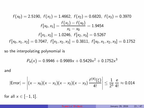
f (x0) = 2.5190, f (x1) = 1.4662, f (x2) = 0.6820, f (x3) = 0.3970

f [x0, x1] =f (x1)− f (x0)

x1 − x0= 1.9454

f [x1, x2] = 1.0246, f [x2, x3] = 0.5267

f [x0, x1, x2] = 0.7047, f [x1, x2, x3] = 0.3811, f [x0, x1, x2, x3] = 0.1752

so the interpolating polynomial is

P4(x) = 0.9946 + 0.9989x + 0.5429x2 + 0.1752x3

and

|Error| =∣∣∣∣∣(x − x0)(x − x1)(x − x2)(x − x3)

f (4)(ξ)

4!

∣∣∣∣∣ ≤1

23e

4!≈ 0.014

for all x ∈ [−1, 1].


Conclusions

1 The degree n monic polynomial with the smallest maximum absolutevalue on [−1, 1] is the modified Chebyshev polynomial T̃n(x) and itsmaximum value is 1/2n−1.

2 Hence, the Chebyshev polynomials can be used to minimizeapproximation error by providing optimal interpolation points.

3 If we want to interpolate a function f (x) by a polynomial of degree n

on the interval [−1, 1], the interpolation points which give thesmallest possible error are given by the zeros of the Chebyshevpolynomial of degree n + 1, Tn+1(x).


Change of interval

The linear transformation

x =b − a

2t +

a + b

2

translates and scales the interval −1 ≤ t ≤ 1 onto the interval a ≤ x ≤ b.

The optimal interpolation points on the interval [a, b] are then given bythe “transformed” zeros of the Chebyshev polynomials,

xk =b − a

2cos

[(2k + 1)π

2n

]+

a + b

2, k = 0, 1, 2, . . . n − 1.

and the following inequality holds on [a, b]:

|(x − x0)(x − x1) · · · (x − xn−1)| ≤(b−a2

)n

2n−1


Review of Taylor series and polynomials

Suppose f (x) is a function on [a, b] which is (n+1)-times differentiable. Ifa ≤ x0 ≤ b then f (x) can be approximated by its n-th Taylor polynomial

f (x) ≈ Pn(x)

= f (x0) + f ′(x0)(x − x0) +f ′′(x0)

2(x − x0)

2 + · · ·+ f (n)(x0)

n!(x − x0)

n

with approximation error (also called the remainder term)

Rn(x) =f (n+1)(ξ)

(n + 1)!(x − x0)

n+1

where ξ is a number between x0 and x .

Hencef (x) = Pn(x) + Rn(x)


Examples

The infinite series obtained from Pn(x) as n → ∞ is called Taylor series off (x) about x0.In the case x0 = 0, the Taylor polynomials/series are often calledMacLaurin polynomials/series.

The Taylor/MacLaurin series for some standard functions are as follows

ex = 1 + x +

x2

2!+ · · · + xn

n!+ · · ·

sin(x) = x − x3

3!+ · · · + (−1)n

x2n+1

(2n + 1)!+ · · ·

cos(x) = 1− x2

2!+

x4

4!+ · · ·+ (−1)n

x2n

(2n)!+ · · ·


Exercises

1 Find the third Taylor polynomial P3(x) for the functionf (x) =

√x + 1 about x0 = 0. Approximate

√0.75 using this

polynomial. Find an error bound for this approximation and compareit with the actual error.

2 Find the second Taylor polynomial P2(x) for the functionf (x) = e

x cos(x) about x0 = 0. Approximate f (0.5) using thispolynomial. Find an error bound for this approximation and compareit with the actual error.

3 Let f (x) = cos(x). Write down the second and third MacLaurinpolynomial for f (x) and the corresponding remainder terms.

4 Find the third Taylor polynomial P3(x) for f (x) = (x − 1) ln(x) aboutx0 = 1. Approximate f (0.5) using P3(0.5). Find an upper bound forthe approximation error using the Taylor remainder term and compareit to the actual error.


Applications of Chebyshev polynomials: Economization of

power series

Given a function f (x) we know how to approximate this function by aninterpolating polynomial Pn(x), using either equally spaced interpolationpoints or the zeros of an appropriate Chebyshev polynomial.(Recall that the latter approach has the advantage of minimizing theapproximation error.)

The question now is how to approximate a given function f (x) by apolynomial of lowest possible degree, which satisfies a certain error bound.

Since every continuous function can be approximated by a Taylor (orMacLaurin) polynomial, we need to learn how to approximate a polynomialby a polynomial of smaller degree.


Approximating a given polynomial by a smaller degree

polynomial

Consider approximating a polynomial of degree n

Pn(x) = anxn + an−1x

n−1 + · · ·+ a1x + a0

on [−1, 1] with a polynomial of degree at most n − 1. We need to choosePn−1(x) which minimizes

maxx∈[−1,1]

|Pn(x)− Pn−1(x)|

Note that (Pn(x)− Pn−1(x))/an is a monic polynomial of degree n. If thispolynomial is to have the smallest possible maximum absolute value thenit needs to be equal to the modified Chebyshev polynomial of degree n,T̃n(x). This minimax error is then equal to 1/2n−1.


Hence we have1

an(Pn(x)− Pn−1(x)) = T̃n(x)

soPn−1(x) = Pn(x)− anT̃n(x)

and this choice gives

maxx∈[−1,1]

|Pn(x) − Pn−1(x)| =|an|2n−1

In conclusion, the approximating polynomial Pn−1 which minimizes theerror has to be chosen as Pn−1(x) = Pn(x) − anT̃n(x).


General economization procedureProblem: Suppose we need to approximate f (x) by a polynomial Pn(x) ofsmallest possible degree such that the approximation error satisfies

|f (x)− Pn(x) < ε

Step 1: Suppose we can find a polynomial Pn(x) such that|f (x)− Pn(x) < ε (for example, a Taylor polynomial).

Step 2: Now try to find a polynomial of degree n − 1, Pn−1, whichsatisfies the same error requirement. Since

|f (x)− Pn−1(x)| < |f (x)− Pn(x)|+ |Pn(x)− Pn−1(x)|

the second term on the right should be as small as possible, thereforeusing the procedure detailed above, we choose

Pn−1(x) = Pn(x)− anT̃n(x)


Step 3: Check the error |f (x)− Pn−1(x)|. If it is still less than ε thenrepeat Step 2 and try to find a polynomial of degree n− 2, using the sameprocedure. If it now exceeds ε then the smallest degree polynomial whichsatisfies the required error bound is Pn(x).

Example:

Starting with the fourth-order MacLaurin polynomial, find the polynomialof least degree which best approximates the function f (x) = e

x on [−1, 1]while keeping the error less than 0.05.


Solution:The function f (x) = e

x can be written as

f (x) = P4(x) + R4(x)

where

P4(x) = 1 + x +x2

2+

x3

6+

x4

24, R4(x) =

x5

120f (5)(ξ)

We see that |R4(x)| ≤ e/120 ≈ 0.023 < 0.05 for all −1 ≤ x ≤ 1.The polynomial of degree 3 which approximates P4(x) with the smallestpossible error is

P3(x) = P4(x)− a4T̃4(x)

=

(1 + x +

x2

2+

x3

6+

x4

24

)− 1

24

(x4 − x2 +

1

8

)

=191

192+ x +

13

24x2 +

1

6x3


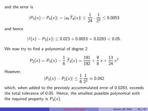
and the error is

|P3(x)− P4(x)| = |a4T̃4(x)| ≤1

24· 1

23≤ 0.0053

and hence

|f (x) − P3(x)| ≤ 0.023 + 0.0053 = 0.0283 < 0.05.

We now try to find a polynomial of degree 2

P2(x) = P3(x)−1

6T̃3(x) =

191

192+

9

8x +

13

24x2

However,

|P3(x)− P2(x)| ≤1

6

1

22≈ 0.042

which, when added to the previosly accummulated error of 0.0283, exceedsthe total tolerance of 0.05. Hence, the smallest possible polynomial withthe required property is P3(x).


Exercises

1 Find the sixth order MacLaurin polynomial for sin(x) and useChebyshev polynomials to obtain a lesser degree polynomialapproximation while keeping the error less than 0.01 on [−1, 1].

2 Same problem for f (x) = xex on [−1, 1].


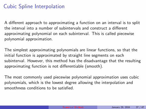
Cubic Spline Interpolation

A different approach to approximating a function on an interval is to splitthe interval into a number of subintervals and construct a differentapproximating polynomial on each subinterval. This is called piecewisepolynomial approximation.

The simplest approximating polynomials are linear functions, so that theinitial function is approximated by straight line segments on eachsubinterval. However, this method has the disadvantage that the resultingapproximating function is not differentiable (smooth).

The most commonly used piecewise polynomial approximation uses cubicpolynomials, which is the lowest degree allowing the interpolation andsmoothness conditions to be satisfied.


Cubic splines

Definition: Given a function f (x) on an interval [a, b] and a set of nodesa = x0 < x1 < x2 < · · · , xn = b, a cubic spline interpolant, S , for f (x)is a function which satisfies the following conditions:

1 S(x) = Sj(x) on each subinterval [xj , xj+1], where Sj is the cubicpolynomial

Sj(x) = aj + bj(x − xj) + cj(x − xj)2 + dj(x − xj)

3

2 Sj(xj ) = f (xj) and Sj(xj+1) = f (xj+1) for each j = 0, 1, . . . , n − 1.

3 Sj+1(xj+1) = Sj(xj+1) for each j = 0, 1, . . . , n − 2.

4 S ′j+1(xj+1) = S ′

j (xj+1) for each j = 0, 1, . . . , n − 2.

5 S ′′j+1(xj+1) = S ′′

j (xj+1) for each j = 0, 1, . . . , n − 2.


Notes

Condition (2) above means that S interpolates the function f (x) at eachof the nodes x0, x1 ... xn. Conditions (3)–(5) state that S and itsderivatives are continuous on [a, b].

Note that the function S consists of n cubic polynomials, each having 4unknown coefficients. There are a total of 4n unknowns to be determined.

The interpolation condition provides n + 1 equations. The 3 continuityconditions provide an additional 3(n-1) equations. To completelydetermine the interpolant, two more conditions are required. These areapplied at the boundary points a and b:

6 One of the following boundary conditions is satisfied at x = a, b:1 S ′′(x0) = S ′′(xn) = 0 (natural or free boundary)2 S ′(x0) = f ′(x0) and S ′(xn) = f ′(xn) (clamped boundary)


Example

Construct a natural cubic spline passing through the points (1, 2), (2, 3)and (3, 5).

We need to construct two cubic polynomials, one for [1, 2]:

S0(x) = a0 + b0(x − 1) + c0(x − 1)2 + d0(x − 1)3

and one for the interval [2, 3]:

S1(x) = a1 + b1(x − 2) + c1(x − 2)2 + d1(x − 2)3

We need 8 equations to determine the 8 unknown constants. The first 4are interpolations conditions:

2 = f (1) = S0(1) = a0, 3 = f (2) = S0(2) = a0 + b0 + c0 + d0

3 = f (2) = S1(2) = a1, 5 = f (3) = S1(3) = a1 + b1 + c1 + d1


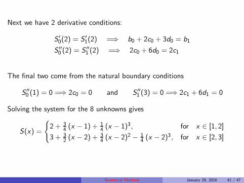
Next we have 2 derivative conditions:

S ′0(2) = S ′

1(2) =⇒ b0 + 2c0 + 3d0 = b1

S ′′0 (2) = S ′′

1 (2) =⇒ 2c0 + 6d0 = 2c1

The final two come from the natural boundary conditions

S ′′0 (1) = 0 =⇒ 2c0 = 0 and S ′′

1 (3) = 0 =⇒ 2c1 + 6d1 = 0

Solving the system for the 8 unknowns gives

S(x) =

{2 + 3

4 (x − 1) + 14 (x − 1)3, for x ∈ [1, 2]

3 + 32 (x − 2) + 3

4 (x − 2)2 − 14 (x − 2)3, for x ∈ [2, 3]


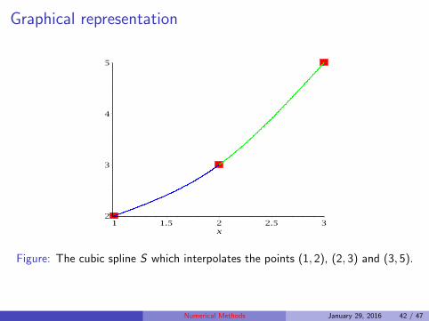
Graphical representation

Figure: The cubic spline S which interpolates the points (1, 2), (2, 3) and (3, 5).


Example 2Now construct a clamped cubic spline passing through the points (1, 2),(2, 3) and (3, 5), which has S ′(1) = 2 and S ′(3) = 1.

Let the cubic polynomials for [1, 2] and [2, 3] be given by

S0(x) = a0 + b0(x − 1) + c0(x − 1)2 + d0(x − 1)3

S1(x) = a1 + b1(x − 2) + c1(x − 2)2 + d1(x − 2)3

The first 6 conditions are the same as in the previous example. However,the two boundary conditions are now

S ′0(1) = 2 =⇒ b0 = 2 and S ′

1(3) = 1 =⇒ b1 + 2c1 + 3d1 = 1.

The spline is now obtained as

S(x) =

{2 + 2 (x − 1)− 5

2 (x − 1)2 + 32 (x − 1)3, for x ∈ [1, 2]

3 + 32 (x − 2) + 2 (x − 2)2 − 3

2 (x − 2)3, for x ∈ [2, 3]


Uniqueness of cubic spline interpolant

If f is defined at a = x0 < x1 < · · · xn = b, then there is a unique splineinterpolant for f on these nodes which satisfies the natural boundaryconditions S ′′(a) = 0 and S ′′(b) = 0.

If f is defined at a = x0 < x1 < · · · xn = b and differentiable at a and b,then there is a unique spline interpolant for f on these nodes whichsatisfies the clamped boundary conditions S ′(a) = f ′(a) and S ′(b) = f ′(b).


Spline interpolation error

The following error bound formula holds for a clamped cubic spline.

Let f be a function on [a, b] which is 4 times differentiable andmaxa≤x≤b |f (4)(x)| = M. If S is the unique clamped cubic splineinterpolant for f (x) with respect to the nodes a = x0 < x1 · · · xn = b thenwe have

|f (x)− S(x)| ≤ 5M

384max

0≤j≤n−1(xj+1 − xj)

4

for all x ∈ [a, b].

A similar formula holds for natural cubic splines but is more difficult toexpress.


Example

Consider the function f (x) = ex on [0, 3] and the nodes x0 = 0, x1 = 1,

x2 = 2 and x3 = 3.

1 Find a natural spline interpolant for f on these nodes.

2 Find a clamped spline interpolant for f on these nodes.

3 Calculate the error of each approximation at x = 2.5 and comparewith the error bound obtained for the clamped spline.


The natural cubic spline is given by

S(x) =

1 + 1.466 x + 0.252 x3, [0, 1]

2.718 + 2.223 (x − 1) + 0.757 (x − 1)2 + 1.691 (x − 1)3, [1, 2]

7.389 + 8.810 (x − 2) + 5.830 (x − 2)2 − 1.943 (x − 2)3, [2, 3]

Figure: The cubic spline S (green) which interpolates the function ex (black).


part ii: interpolation and approximation theorydmackey/lectures/interpolationii.pdf · polynomial...

Documents