Part II

Time Series

12 Introduction

This Part is mainly a summary of the book of Brockwell and Davis (2002). Additionallythe textbook Shumway and Stoffer (2010) can be recommended.1

Our purpose is to study techniques drawing inferences from time series. Before wecan do this, it is necessary to set up a hypothetical probability model to represent thedata. After an appropriate family of models has been chosen, it is then possible toestimate parameters, check for goodness of fit to the data, and possibly to use the fittedmodel to enhance our understanding of the mechanism generating the series. Once asatisfactory model has been developed, it may be used in a variety of ways dependingon the particular field of application.

12.1 Definitions and Examples

Definition 12.1.1. A time series is a set of observations xt each one being recorded at aspecific time t. A discrete time series is one in which the set T0 of times at which observa-tions are made is a discrete set. Continuous time series are obtained when observationsare recorded continuously over some time interval.

Example. Some examples of discrete univariate time series from climate sciences andenergy markets are shown on pages 12-2 to 12-4.

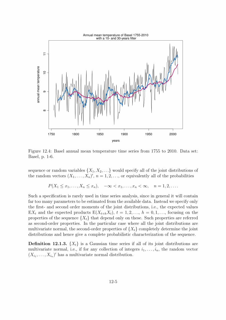
Example (Basel, p. 1-6). We come back to the Basel temperature time series whichstarts in 1755 and is the longest temperature time series in Switzerland. We will analyzethis data set and try to find an adequate time series model. To get an overview westart with Figure 12.4 showing the annual mean temperatures from 1755 to 2010. Witha boxplot (see Figure 12.5, p. 12-6) the monthly variability, called seasonality, but alsothe intermonthly variability can be shown. Finally Figure 12.6, p. 12-7, shows themonthly temperature time series from 1991 to 2010.

An important part of the analysis of a time series is the selection of a suitableprobability model for the data. To allow for the possibly unpredictable nature of futureobservations it is natural to suppose that each observation xt is a realized value of acertain random variable Xt.

Definition 12.1.2. A time series model for the observed data {xt} is a specificationof the joint distribution (or possibly only the means and covariances) of a sequence ofrandom variables {Xt} of which {xt} is postulated to be a realization.

Remark. We shall frequently use the term time series to mean both the data and theprocess of which it is a realization. A complete probabilistic time series model for the

1http://www.stat.pitt.edu/stoffer/tsa3/ (12.04.2015).

12-1

Figure 12.1: Global development of the atmospheric CO2 concentration, annual meantemperature and sea level from 1850 to 2010. Source: OcCC (2008).

12-2

Abw

eic

hung °

C

−2.0

−1.5

−1.0

−0.5

0.0

0.5

1.0

1.5

2.0

2.5

1880 1900 1920 1940 1960 1980 2000

Jahres−Temperatur Mittel(BAS,BER,CHD,CHM,DAV,ENG,GVE,LUG,SAE,SIA,SIO,SMA) 1864−2014

Abweichung vom Durchschnitt 1961−1990

Abw

eic

hung °

C

Jahre über dem Durchschnitt 1961−1990

Jahre unter dem Durchschnitt 1961−1990

20−jähriges gewichtetes Mittel (Gauss Tiefpassfilter)

© MeteoSchweiz

homogval.evol 2.11.12 / 31.01.2015, 10:50

Verh

ältnis

0.5

0.6

0.7

0.8

0.9

1

1.1

1.2

1.3

1.4

1880 1900 1920 1940 1960 1980 2000

Jahres−Niederschlag Mittel(BAS,BER,CHD,CHM,DAV,ENG,GVE,LUG,SAE,SIA,SIO,SMA) 1864−2014

Verhältnis zum Durchschnitt 1961−1990

Verh

ältnis

Jahre über dem Durchschnitt 1961−1990

Jahre unter dem Durchschnitt 1961−1990

20−jähriges gewichtetes Mittel (Gauss Tiefpassfilter)

© MeteoSchweiz

homogval.evol 2.11.12 / 31.01.2015, 10:51

Figure 12.2: Time series from 1864 to 2014 of the anomalies from the reference period1961-1990 of the annual mean temperature in Switzerland (top) and the precipitationin Southern Switzerland (bottom). Source: MeteoSchweiz.

12-3

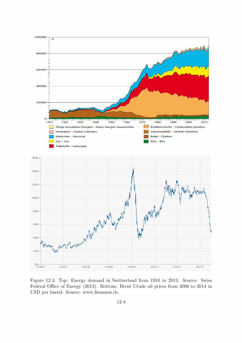
Figure 12.3: Top: Energy demand in Switzerland from 1910 to 2013. Source: SwissFederal Office of Energy (2013). Bottom: Brent Crude oil prices from 2000 to 2014 inUSD per barrel. Source: www.finanzen.ch.

12-4

years

an

nu

al m

ea

n t

em

pe

ratu

re

1750 1800 1850 1900 1950 2000

89

10

11

Annual mean temperature of Basel 1755-2010 with a 10- and 30-years filter

Figure 12.4: Basel annual mean temperature time series from 1755 to 2010. Data set:Basel, p. 1-6.

sequence or random variables {X1, X2, . . .} would specify all of the joint distributions ofthe random vectors (X1, . . . , Xn)′, n = 1, 2, . . ., or equivalently all of the probabilities

P (X1 ≤ x1, . . . , Xn ≤ xn), −∞ < x1, . . . , xn <∞, n = 1, 2, . . . .

Such a specification is rarely used in time series analysis, since in general it will containfar too many parameters to be estimated from the available data. Instead we specify onlythe first- and second order moments of the joint distributions, i.e., the expected valuesEXt and the expected products E(Xt+hXt), t = 1, 2, . . ., h = 0, 1, . . ., focusing on theproperties of the sequence {Xt} that depend only on these. Such properties are referredas second-order properties. In the particular case where all the joint distributions aremultivariate normal, the second-order properties of {Xt} completely determine the jointdistributions and hence give a complete probabilistic characterization of the sequence.

Definition 12.1.3. {Xt} is a Gaussian time series if all of its joint distributions aremultivariate normal, i.e., if for any collection of integers i1, . . . , in, the random vector(Xi1 , . . . , Xin)′ has a multivariate normal distribution.

12-5

-10

01

02

0

Jan Feb Mar Apr May Jun Jul Aug Sep Oct Nov Dec

Temperature of Basel 1755-2010

Figure 12.5: Boxplot of the Basel monthly mean temperature time series from 1755 to2010. Data set: Basel, p. 1-6.

12.2 Simple Time Series Models

12.2.1 Zero-mean Models

We introduce some important time series models.

� Independent and identically distributed (iid) noise: Perhaps the simplest modelfor a time series is one in which there is no trend or seasonal component andin which the observations are simply independent and identically distributed (iid)random variables with zero mean. We refer to such a sequence of random variablesX1, X2, . . . as iid noise. By definition we can write, for any positive integer n andreal numbers x1, . . . , xn,

P (X1 ≤ x1, . . . , Xn ≤ xn) = P (X1 ≤ x1) · . . . · P (Xn ≤ xn) = F (x1) · · ·F (xn),

where F (·) is the cumulative distribution function of each of the identically dis-tributed random variables X1, X2, . . .. In this model there is no dependence be-tween observations. In particular, for all h ≥ 1 and all x, x1, . . . , xn,

P (Xn+h ≤ x|X1 = x1, . . . , Xn = xn) = P (Xn+h ≤ x),

showing that knowledge of X1, . . . , Xn is of no value for predicting the behavior ofXn+h.

12-6

Monthly temperature of Basel

1991 1992 1993 1994 1995 1996 1997 1998 1999 2000 2001 2002 2003 2004 2005 2006 2007 2008 2009 2010 2011

05

10

15

20

Figure 12.6: Basel monthly mean temperature time series from 1991 to 2010. Data set:Basel, p. 1-6.

Remark. We shall use the notation

{Xt} ∼ IID(0, σ2)

to indicate that the random variables Xt are independent and identically dis-tributed random variables, each with mean 0 and variance σ2.

Although iid noise is a rather uninteresting process for forecasting, it plays animportant role as a building block for more complicated time series models.

� Binary process: Consider the sequence of iid random variables {Xt, t = 1, 2, . . .}with

P (Xt = 1) = p, P (Xt = −1) = 1− p,where p = 1/2.

� Random walk: The random walk {St, t = 0, 1, 2, . . .} is obtained by cumulativelysumming iid random variables. Thus a random walk with zero mean is obtainedby defining

S0 = 0 and St = X1 + . . .+Xt for t = 1, 2, . . . ,

where {Xt} is iid noise.

12-7

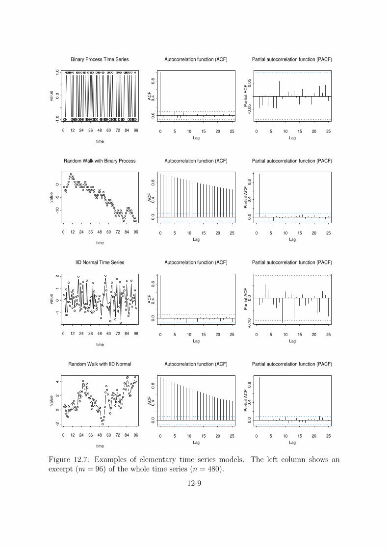
Example. Figure 12.7 shows different examples of zero-mean time series models.

12.2.2 Models with Trend and Seasonality

In several of the time series there is a clear trend in the data. In these cases a zero-meanmodel for the data is clearly inappropriate.

� Trend: Xt = mt + Yt, where mt is a slowly changing function known as the trendcomponent and Yt has zero mean. A useful technique for estimating mt is themethod of least squares.

Example. In the least squares procedure we attempt to fit a parametric familyof functions, e.g., mt = a0 + a1t + a2t

2 to the data {x1, . . . , xn} by choosing theparameters a0, a1 and a2 to minimize

n∑

t=1

(xt −mt)2

� Seasonality: In order to represent a seasonal effect, allowing for noise but assumingno trend, we can use the simple model

Xt = st + Yt,

where st is a periodic function of t with period d, i.e., st−d = st.

Example. A convenient choice for st is a sum of harmonics given by

st = a0 +k∑

j=1

(aj cos(λjt) + bj sin(λjt))

where a0, . . . , ak and b1, . . . , bk are unknown parameters and λ1, . . . , λk are fixedfrequencies, each being some integer multiple of 2π/d.

12.3 General Approach to Time Series Modeling

The examples of the previous section illustrate a general approach to time series anal-ysis. Before introducing the ideas of dependence and stationarity, the following outlineprovides the reader with an overview of the way in which the various ideas fit together:

1. Plot the series and examine the main features of the graph, checking in particularwhether there is

(a) a trend,

(b) a seasonal component,

12-8

time

valu

e

-1.0

0.0

1.0

0 12 24 36 48 60 72 84 96

Binary Process Time Series

Lag

AC

F

0 5 10 15 20 25

0.0

0.4

0.8

Autocorrelation function (ACF)

Lag

Part

ial A

CF

0 5 10 15 20 25

-0.0

50.0

5

Partial autocorrelation function (PACF)

time

valu

e

-10

-50

0 12 24 36 48 60 72 84 96

Random Walk with Binary Process

Lag

AC

F

0 5 10 15 20 25

0.0

0.4

0.8

Autocorrelation function (ACF)

Lag

Part

ial A

CF

0 5 10 15 20 25

0.0

0.4

0.8

Partial autocorrelation function (PACF)

time

valu

e

-10

12

0 12 24 36 48 60 72 84 96

IID Normal Time Series

Lag

AC

F

0 5 10 15 20 25

0.0

0.4

0.8

Autocorrelation function (ACF)

Lag

Part

ial A

CF

0 5 10 15 20 25

-0.1

00.0

Partial autocorrelation function (PACF)

time

valu

e

-20

24

0 12 24 36 48 60 72 84 96

Random Walk with IID Normal

Lag

AC

F

0 5 10 15 20 25

0.0

0.4

0.8

Autocorrelation function (ACF)

Lag

Part

ial A

CF

0 5 10 15 20 25

0.0

0.4

0.8

Partial autocorrelation function (PACF)

Figure 12.7: Examples of elementary time series models. The left column shows anexcerpt (m = 96) of the whole time series (n = 480).

12-9

(c) any apparent sharp changes in behavior,

(d) any outlying observations.

Example (Basel, p. 1-6). The Basel annual mean temperature time series (Figure12.4, p. 12-5) does not have an obvious trend for the first period till 1900 whilefor the second period, starting with the 20th century a linear upward trend can beobserved. Furthermore the Basel monthly mean temperature time series (Figure12.5, p. 12-6) shows a strong seasonal component.

2. Remove the trend and seasonal components to get stationary residuals (see Section12.4). To achieve this goal it may sometimes be necessary to apply a preliminarytransformation to the data. There are several ways in which trend and seasonalitycan be removed (see Section 12.5).

3. Choose a model to fit the residuals.

4. Forecasting will be achieved by forecasting the residuals and then inverting thetransformations described above to arrive at forecasts of the original series {Xt}.

12.4 Stationary Models and the Autocorrelation Func-

tion

Loosely speaking, a time series {Xt, t = 0,±1,±2, . . .} is said to be stationary if it hasstatistical properties similar to those of the “time-shifted” series {Xt+h, t = 0,±1,±2, . . .},for each integer h. So stationarity implies that the model parameters do not vary withtime. Restricting attention to those properties that depend only on the first- and second-order moments of {Xt}, we can make this idea precise with the following definitions.

Definition 12.4.1. Let {Xt} be a time series with E(X2t ) <∞. The mean function of

{Xt} isµX(t) = E(Xt).

The covariance function of {Xt} is

γX(r, s) = Cov(Xr, Xs) = E((Xr − µX(r))(Xs − µX(s)))

for all integers r and s.

Definition 12.4.2. {Xt} is (weakly) stationary if

� the mean value function µX(t) is constant and does not depend on time t and

� the autocovariance function γX(r, s) depends on r and s only through their differ-ence |r − s|, or in other words γX(t+ h, t) is independent of t for each h.

12-10

Remark. A strictly stationary time series is one for which the probabilistic behaviorof every collection of values {x1, . . . xn} is identical to that of the time shifted set{x1+h, . . . xn+h}. That is, strict stationarity of a time series {Xt, t = 0,±1,±2, . . .}is defined by the condition that (X1, . . . , Xn) and (X1+h, . . . , Xn+h) have the same jointdistributions for all integers h and n > 0. It can be checked that if {Xt} is strictlystationary and EX2

t < ∞ for all t, then {Xt} is also weakly stationary. Whenever weuse the term stationary we shall mean weakly stationary as in Definition 12.4.2.

Remark. If a Gaussian time series is weakly stationary it is also strictly stationary.

Remark. Whenever we use the term covariance function with reference to a stationarytime series {Xt} we define

γX(h) := γX(h, 0) = γX(t+ h, t).

The function γX(·) will be referred to as the autocovariance function and γX(h) as itsvalue at lag h.

Definition 12.4.3. Let {Xt} be a stationary time series. The autocovariance function(ACFV) of {Xt} at lag h is

γX(h) = Cov(Xt+h, Xt) = E(Xt+hXt)− EXt+hEXt.

The autocorrelation function (ACF) of {Xt} at lag h is

ρX(h) :=γX(h)

γX(0)= Cor(Xt+h, Xt).

Example. Let’s have a look to some zero-mean time series models (compare Figure12.7):

� iid noise: If {Xt} is iid noise and E(X2t ) = σ2 < ∞, then the first requirement of

Definition 12.4.2 is satisfied since E(Xt) = 0, for all t. By the assumed indepen-dence

γX(t+ h, t) =

{σ2, if h = 0,

0, if h 6= 0.

which does not depend on t. Hence iid noise with finite second moment is station-ary. We shall use the notation

{Xt} ∼ IID(0, σ2)

to indicate that the random variables Xt are independent and identically dis-tributed random variables, each with mean 0 and variance σ2.

� White noise: If {Xt} is a sequence of uncorrelated random variables, each with zeromean and variance σ2, then {Xt} is stationary with the same covariance functionas the iid noise. Such a sequence is referred to as white noise (with mean 0 andvariance σ2). This is indicated by the notation

{Xt} ∼WN(0, σ2).

12-11

Remark. Every IID(0, σ2) sequence is WN(0, σ2) but not conversely: Let {Zt} ∼N(0, 1) and define

Xt =

{Zt, t even,

(Z2t−1 − 1)/

√2, t odd,

then {Xt} ∼WN(0, 1) but not IID(0, 1).

� Random walk: We find ESt = 0, ES2t = tσ2 <∞ for all t, and, for h ≥ 0,

γS(t+ h, t) = Cov(St+h, St) = tσ2.

Since γS(t+ h, t) depends on t, the series {St} is not stationary.

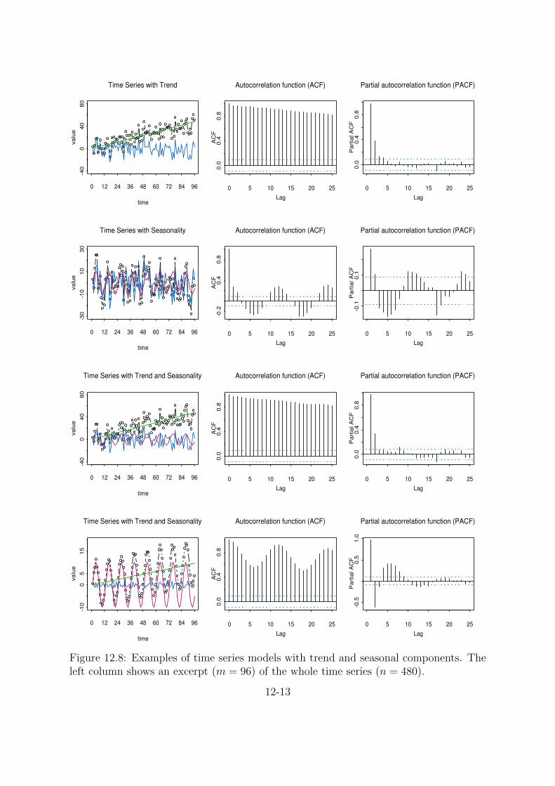
Example. Figure 12.8 shows different examples of time series models with trend andseasonal components.

Example. First-order moving average or MA(1) process: Consider the series defined bythe equation

Xt = Zt + θZt−1, t = 0,±1,±2, . . . , (12.1)

where {Zt} ∼WN(0, σ2) and θ is a real-valued constant. We find EXt = 0 and EX2t =

σ2(1 + θ2) <∞. The autocovariance function can be calculated as

γX(t+ h, t) =

σ2(1 + θ2), if h = 0,

σ2θ, if h = ±1,

0, if |h| > 1.

(12.2)

Therefore {Xt} is stationary.

Example. Note that the processes Xt = Zt + 5Zt−1, where {Zt} ∼ WN(0, 1) andYt = Wt + 1

5Wt−1, where {Wt} ∼ WN(0, 25) have the same autocovariance functions.

Since we can only observe the time series Xt or Yt and not the noise Zt or Wt wecannot distinguish between the models. But as we will see later on, the second model isinvertible, while the first is not.

Example. First-order autoregression or AR(1) process: Let us assume that the series{Xt} defined by the equation

Xt = φXt−1 + Zt, t = 0,±1,±2, . . . , (12.3)

is stationary, where {Zt} ∼ WN(0, σ2), Zt is uncorrelated with Xs for each s < t and|φ| < 1.

By taking expectations on each side of (12.3) and using the fact that EZt = 0, wesee at once that EXt = 0. To find the autocovariance function of {Xt} multiply eachside of (12.3) by Xt−h and then take expectations to get

γX(h) = Cov(Xt, Xt−h) = Cov(φXt−1, Xt−h) + Cov(Zt, Xt−h)

= φγX(h− 1) = . . . = φhγX(0).

12-12

time

valu

e

-40

040

80

0 12 24 36 48 60 72 84 96

Time Series with Trend

Lag

AC

F

0 5 10 15 20 25

0.0

0.4

0.8

Autocorrelation function (ACF)

Lag

Part

ial A

CF

0 5 10 15 20 25

0.0

0.4

0.8

Partial autocorrelation function (PACF)

time

valu

e

-30

-10

10

30

0 12 24 36 48 60 72 84 96

Time Series with Seasonality

Lag

AC

F

0 5 10 15 20 25

-0.2

0.4

0.8

Autocorrelation function (ACF)

Lag

Part

ial A

CF

0 5 10 15 20 25

-0.1

0.1

Partial autocorrelation function (PACF)

time

valu

e

-40

040

80

0 12 24 36 48 60 72 84 96

Time Series with Trend and Seasonality

Lag

AC

F

0 5 10 15 20 25

0.0

0.4

0.8

Autocorrelation function (ACF)

Lag

Part

ial A

CF

0 5 10 15 20 25

0.0

0.4

0.8

Partial autocorrelation function (PACF)

time

valu

e

-10

05

15

0 12 24 36 48 60 72 84 96

Time Series with Trend and Seasonality

Lag

AC

F

0 5 10 15 20 25

0.0

0.4

0.8

Autocorrelation function (ACF)

Lag

Part

ial A

CF

0 5 10 15 20 25

-0.5

0.5

1.0

Partial autocorrelation function (PACF)

Figure 12.8: Examples of time series models with trend and seasonal components. Theleft column shows an excerpt (m = 96) of the whole time series (n = 480).

12-13

Observing that γ(h) = γ(−h), we find that

ρX(h) =γX(h)

γX(0)= φ|h|, h = 0,±1, . . . .

It follows from the linearity of the covariance function and the fact that Zt is uncorrelatedwith Xt−1 that

γX(0) = Cov(Xt, Xt) = Cov(φXt−1 + Zt, φXt−1 + Zt) = φ2γX(0) + σ2

and hence that

γX(0) =σ2

1− φ2.

Combined we have

γX(h) = φ|h|σ2

1− φ2.

For more details on AR(1) processes see page 13-6.

Definition 12.4.4. Let x1, . . . , xn be observations of a time series. The sample meanof x1, . . . , xn is

x =1

n

n∑

j=1

xj.

For |h| < n we define the sample autocovariance function

γ̂(h) :=1

n

n−|h|∑

j=1

(xj+|h| − x)(xj − x),

and the sample autocorrelation function

ρ̂(h) =γ̂(h)

γ̂(0).

Remark. For data containing a trend, |ρ̂(h)| will exhibit slow decay as h increases, andfor data with a substantial deterministic periodic component, |ρ̂(h)| will exhibit similarbehavior with the same periodicity (see Figure 12.8). Thus ρ̂(·) can be useful as anindicator of nonstationarity.

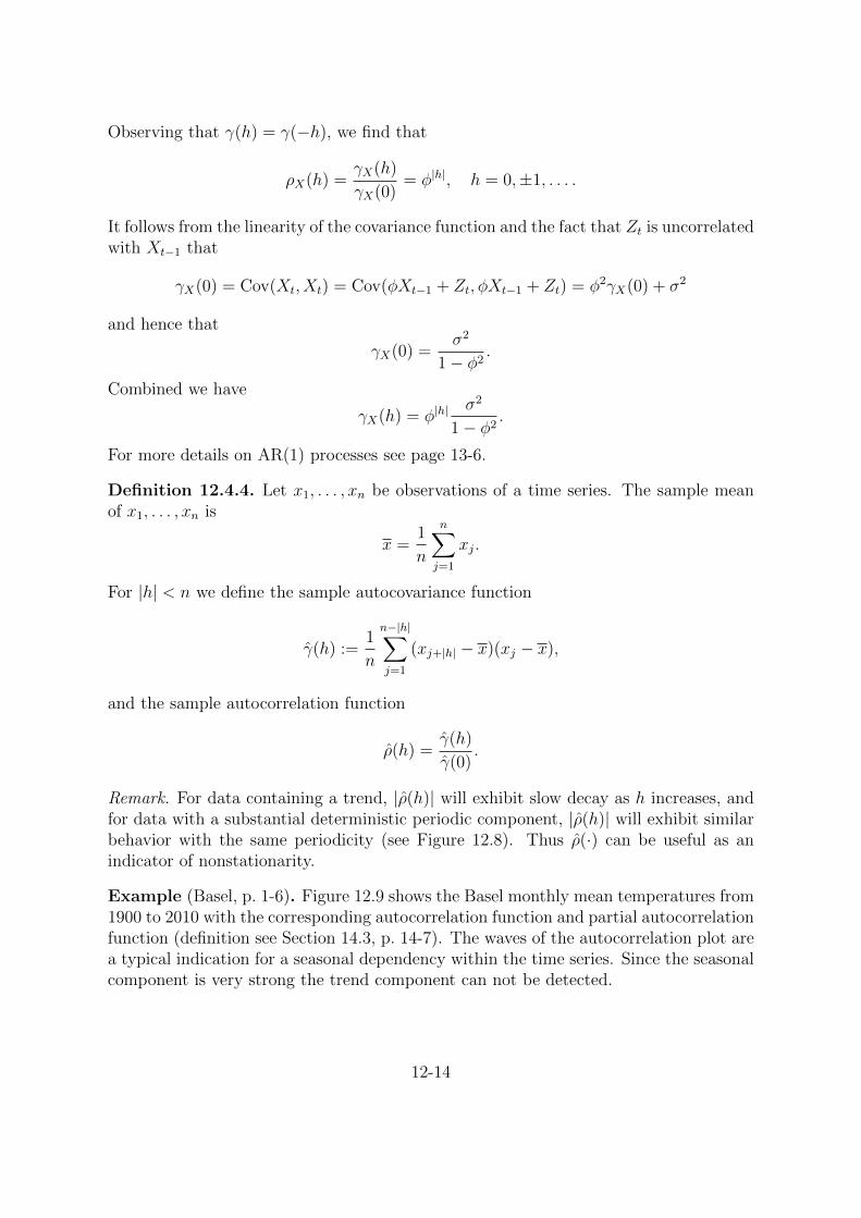
Example (Basel, p. 1-6). Figure 12.9 shows the Basel monthly mean temperatures from1900 to 2010 with the corresponding autocorrelation function and partial autocorrelationfunction (definition see Section 14.3, p. 14-7). The waves of the autocorrelation plot area typical indication for a seasonal dependency within the time series. Since the seasonalcomponent is very strong the trend component can not be detected.

12-14

Time series

Time in months

-10

01

02

0

Jan 1900 Jan 1920 Jan 1940 Jan 1960 Jan 1980 Jan 2000

Lag (in months)

0.0 0.5 1.0 1.5 2.0 2.5

-0.5

0.5

autocorrelation function

Lag (in months)

0.0 0.5 1.0 1.5 2.0 2.5

-0.6

0.0

0.4

0.8

partial autocorrelation function

Figure 12.9: Basel monthly mean temperature time series from 1900 to 2010 with corre-sponding autocorrelation function and partial autocorrelation function. Data set: Basel,p. 1-6.

12.5 Estimation and Elimination of Trend and Sea-

sonal Components

The first step in the analysis of any time series is to plot the data. If there are anyapparent discontinuities in the series, such as a sudden change of level, it may be advis-able to analyze the series by first breaking it into homogeneous segments. If there areoutlying observations, they should be studied carefully to check whether there is anyjustification for discarding them. Inspection of a graph may also suggest the possibilityof representing the data as a realization of the classical decomposition model

Xt = mt + st + Yt, (12.4)

where mt is a slowly changing function known as a trend component, st is a functionwith known period d referred as a seasonal decomposition, and Yt is a random noisecomponent that is stationary. If the seasonal and noise fluctuations appear to increasewith the level of the process, then a preliminary transformation of the data is often usedto make the transformed data more compatible with the model (12.4).

12-15

Our aim is to estimate and extract the deterministic components mt and st in thehope that the residual or noise component Yt will turn out to be a stationary time series(method 1). We can then use the theory of such processes to find a satisfactory proba-bilistic model for the process Yt, to analyze its properties, and to use it in conjunctionwith mt and st for purposes of prediction and simulation of {Xt}.

Another approach is to apply differencing operators repeatedly to the series {Xt}until the differenced observations resemble a realization of some stationary time series{Wt} (method 2). We can then use the theory of stationary processes for the modeling,analysis, and prediction of {Wt} and hence of the original process.

12.5.1 Nonseasonal Model with Trend

In the absence of a seasonal component the model (12.4) becomes

Xt = mt + Yt, t = 1, . . . , n, (12.5)

where EYt = 0.

Method 1: Trend estimation

A lot of methods can be found in literature, here some examples.

a) Smoothing with a finite moving average filter. Let q be a non-negative integer andconsider the two-sided moving average

Wt = (2q + 1)−1q∑

j=−q

Xt−j

of the process {Xt} defined in (12.5). Then for q + 1 ≤ t ≤ n− q, we find

Wt = (2q + 1)−1q∑

j=−q

mt−j + (2q + 1)−1q∑

j=−q

Yt−j ≈ mt,

assuming that mt is approximately linear over the interval [t−q, t+q] and that theaverage of the error terms over this interval is close to zero. The moving averagethus provides us with the estimates

m̂t = (2q + 1)−1q∑

j=−q

Xt−j, q + 1 ≤ t ≤ n− q. (12.6)

b) Exponential smoothing. For any fixed α ∈ [0, 1], the one-sided moving averagesm̂t, t = 1, . . . , n, are defined by the recursions

m̂t = αXt + (1− α)m̂t−1, t = 2, . . . , n,

and

m̂1 = X1.

12-16

c) Smoothing by eliminating high-frequency components.

d) Polynomial fitting. This method can be used to estimate higher-order polynomialtrends.

Method 2: Trend Elimination by Differencing

The trend term is eliminated by differencing. We define the lag-1 difference operator ∇by

∇Xt = Xt −Xt−1 = (1−B)Xt,

where B is the backward shift operator,

BXt = Xt−1.

Powers of the operators B and ∇ are defined in the obvious way, i.e.,

Bj(Xt) = Xt−j,

∇j(Xt) = ∇(∇j−1(Xt)), j ≥ 1, with ∇0(Xt) = Xt.

Example. If the time series {Xt} in (12.5) has a polynomial trend of degree k, it canbe eliminated by application of the operator ∇k:

∇kXt = k! ck +∇kYt,

which gives a stationary process with mean k! ck.

12.5.2 Seasonal Model with Trend

The methods described for the estimation and elimination of trend can be adapted in anatural way to eliminate both trend and seasonality in the general model, specified asfollows.

Xt = mt + st + Yt, t = 1, . . . , n

where

EYt = 0, st+d = st,d∑

j=1

sj = 0.

Method 1: Estimation of trend and seasonal component

Suppose we have observations {x1, . . . , xn}. The trend is first estimated by applyinga moving average filter specially chosen to eliminate the seasonal component and todampen the noise. If the period d is even, say d = 2q, then we use

m̂t = (0.5xt−q + xt−q+1 + . . .+ xt+q−1 + 0.5xt+q)/d, q < t ≤ n− q.If the period is odd, say d = 2q + 1, then we use the simple moving average (12.6). Thesecond step is to estimate the seasonal component.

12-17

Method 2: Elimination of trend and seasonal components by differencing

The technique of differencing that was applied to nonseasonal data can be adaptedto deal with seasonality of period d by introducing the lag-d differencing operator ∇d

defined by∇dXt = Xt −Xt−d = (1−Bd)Xt.

Applying the operator ∇d to the model

Xt = mt + st + Yt,

where {st} has period d, we obtain

∇dXt = mt −mt−d + Yt − Yt−d,which gives a decomposition of the difference ∇dXt into a trend component (mt−mt−d)and a noise term (Yt − Yt−d). The trend, mt −mt−d, can then be eliminated using themethods already described, in particular by applying a power of the operator ∇.

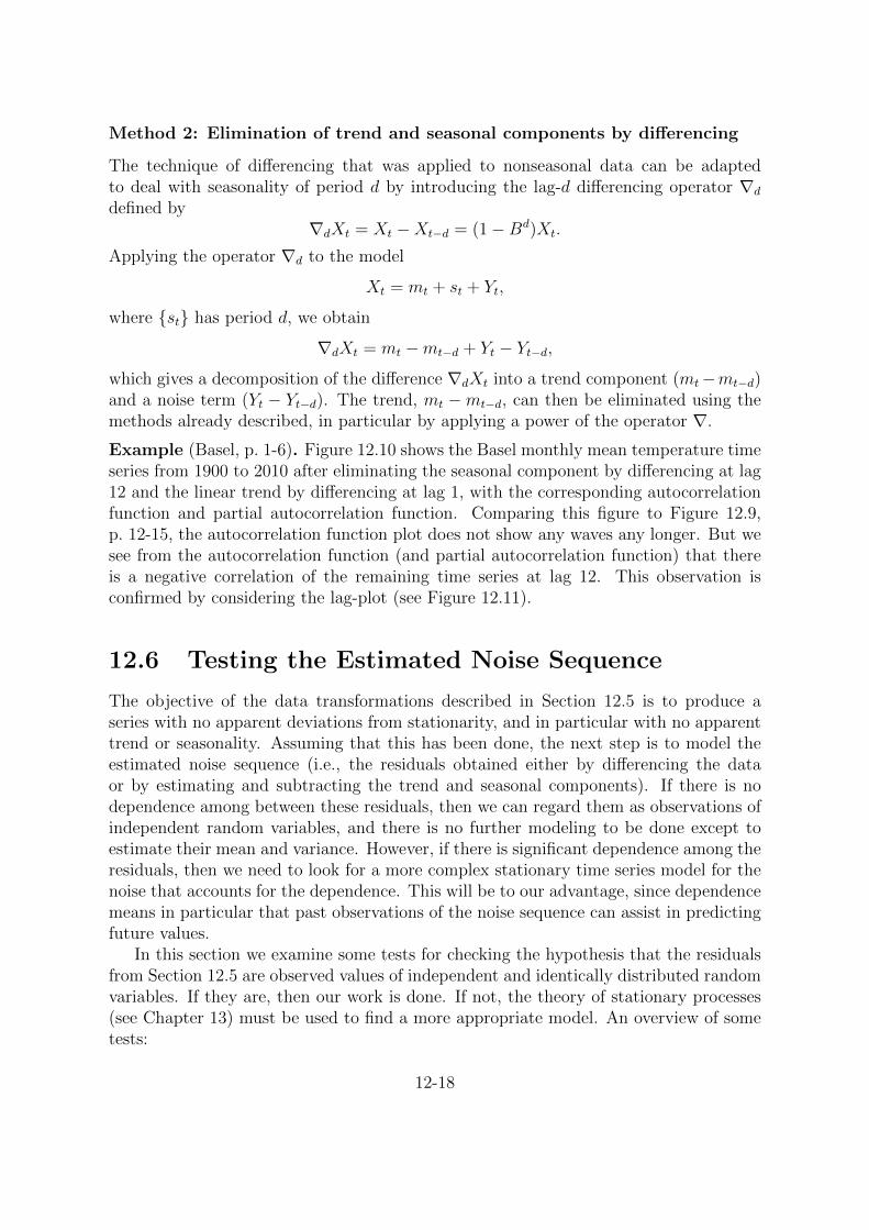
Example (Basel, p. 1-6). Figure 12.10 shows the Basel monthly mean temperature timeseries from 1900 to 2010 after eliminating the seasonal component by differencing at lag12 and the linear trend by differencing at lag 1, with the corresponding autocorrelationfunction and partial autocorrelation function. Comparing this figure to Figure 12.9,p. 12-15, the autocorrelation function plot does not show any waves any longer. But wesee from the autocorrelation function (and partial autocorrelation function) that thereis a negative correlation of the remaining time series at lag 12. This observation isconfirmed by considering the lag-plot (see Figure 12.11).

12.6 Testing the Estimated Noise Sequence

The objective of the data transformations described in Section 12.5 is to produce aseries with no apparent deviations from stationarity, and in particular with no apparenttrend or seasonality. Assuming that this has been done, the next step is to model theestimated noise sequence (i.e., the residuals obtained either by differencing the dataor by estimating and subtracting the trend and seasonal components). If there is nodependence among between these residuals, then we can regard them as observations ofindependent random variables, and there is no further modeling to be done except toestimate their mean and variance. However, if there is significant dependence among theresiduals, then we need to look for a more complex stationary time series model for thenoise that accounts for the dependence. This will be to our advantage, since dependencemeans in particular that past observations of the noise sequence can assist in predictingfuture values.

In this section we examine some tests for checking the hypothesis that the residualsfrom Section 12.5 are observed values of independent and identically distributed randomvariables. If they are, then our work is done. If not, the theory of stationary processes(see Chapter 13) must be used to find a more appropriate model. An overview of sometests:

12-18

Time series

Time in months

-10

05

15

Jan 1900 Jan 1920 Jan 1940 Jan 1960 Jan 1980 Jan 2000

Lag (in months)

0.0 0.5 1.0 1.5 2.0 2.5

-0.5

0.0

0.5

1.0

autocorrelation function

Lag (in months)

0.0 0.5 1.0 1.5 2.0 2.5

-0.4

0.0

0.4

partial autocorrelation function

Figure 12.10: Basel monthly mean temperature time series from 1900 to 2010 after differ-encing at lag 12 for eliminating the seasonal component and at lag 1 for eliminating thelinear trend with the corresponding autocorrelation function and partial autocorrelationfunction.

a) Sample autocorrelation function (SACF): For large n, the SACF of an iid sequenceY1, . . . , Yn with finite variance are approximately iid with N(0, 1/n). Hence, ify1, . . . , yn is a realization of such an iid sequence, about 95% of the sample auto-correlations should fall between the bounds ±1.96/

√n. If we compute the sample

autocorrelations up to lag 40 and find that more than two or three values fall out-side the bounds, or that one value falls far outside the bounds, we therefore rejectthe iid hypothesis.

b) Portmanteau test: Consider the statistic

Q = nh∑

j=1

ρ̂2(j)

where ρ̂ is the sample autocorrelation function. If Y1, . . . , Yn is a finite-variance iidsequence, then Q is approximately distributed as the sum of squares of the inde-pendent N(0, 1) random variables,

√nρ̂(j), j = 1, . . . , h, i.e., as chi-squared with

12-19

lagged 1

Series 1

-10 0 5 10

-10

05

10

lagged 2

Series 1

-10 0 5 10

-10

05

10

lagged 3

Series 1

-10 0 5 10

-10

05

10

lagged 4

Series 1

-10 0 5 10

-10

05

10

lagged 5

Series 1

-10 0 5 10

-10

05

10

lagged 6

Series 1

-10 0 5 10

-10

05

10

lagged 7

Series 1

-10 0 5 10

-10

05

10

lagged 8

Series 1

-10 0 5 10

-10

05

10

lagged 9

Series 1

-10 0 5 10

-10

05

10

lagged 10

Series 1

-10 0 5 10

-10

05

10

lagged 11

Series 1

-10 0 5 10

-10

05

10

lagged 12

Series 1

-10 0 5 10

-10

05

10

Lag-plot of deseasonalized and detrended tempeature of Basel

Figure 12.11: Lag-plot of the Basel monthly mean temperature time series from 1900 to2010 after differencing at lag 12 for eliminating the seasonal component and at lag 1 foreliminating the linear trend.

h degrees of freedom. A large value of Q suggests that the sample autocorrelationsof the data are too large for the data to be a sample from an iid sequence. Wetherefore reject the iid hypothesis at level α if Q > χ2

1−α(h), where χ21−α(h) is the

1− α quantile of the chi-squared distribution with h degrees of freedom.

There exists a refinement of this test, formulated by Ljung and Box, in which Qis replaced by

QLB = n(n+ 2)h∑

j=1

ρ̂2(j)

n− j ,

whose distribution is better approximated by the chi-squared distribution with hdegrees of freedom.

Example (Basel, p. 1-6). Figure 17.1, p. 17-3, shows the Ljung-Box test for theresiduals of the Basel monthly mean temperature time series.

c) The turning point test: If y1, . . . , yn is a sequence of observations, we say thatthere is a turning point at time i, if yi−1 < yi and yi > yi+1 or if yi−1 > yi and

12-20

yi < yi+1. If T is the number of turning points of an iid sequence of length n, then,since the probability of a turning point at time i is 2/3, the expected value of T is

µT = E(T ) =2

3(n− 2).

It can be shown for an iid sequence that the variance of T is

σ2T = Var(T ) =

16n− 29

90.

A large value of T − µT indicates that the series is fluctuating more rapidly thanexpected for an iid sequence. On the other hand, a value T − µT much smallerthan zero indicates a positive correlation between neighboring observations. Foran iid sequence with n large, it can be shown that

Tapprox∼ N(µT , σ

2T ).

This means we carry out a test of the iid hypothesis, rejecting it at level α if|T − µT |/σT > Φ1−α/2, where Φ1−α/2 is the 1 − α/2 quantile of the standardnormal distribution.

d) The difference-sign test: For this test we count the number S of values of i suchthat yi > yi−1, i = 2, . . . , n, or equivalently the number of times the differencedseries yi − yi−1 is positive. For an iid sequence we see that

µS =n− 1

2and σ2

S =n+ 1

12,

and for large n,S

approx∼ N(µS, σ2S).

A large positive (or negative) value of S−µS indicates the presence of an increasing(or decreasing) trend in the data. We therefore reject the assumption of no trendin the data if |S − µS|/σS > Φ1−α/2. The difference-sign test must be used withcaution. A set of observations exhibiting a strong cyclic component will pass thedifference-sign test for randomness, since roughly half of the observations will bepoints of increase.

e) The rank test: This test is particularly useful for detecting a linear trend in thedata. Define P to be the number of pairs (i, j) such that yj > yi and j > i,i = 1, . . . , n − 1. The mean of P is µp = 1

4n(n − 1). A large positive (negative)

value of P − µP indicates the presence of an increasing (decreasing) trend in thedata.

Remark. The general strategy in applying the tests is to check them all and to proceedwith caution if any of them suggests a serious deviation from the iid hypothesis.

12-21