part iii - concordia universitypsychology.concordia.ca/fac/kline/library/k13b.pdfthe difference is...
TRANSCRIPT

Part III
Item-Level Analysis
6241-029-P3-006-2pass-r02.indd 1696241-029-P3-006-2pass-r02.indd 169 1/16/2013 9:14:56 PM1/16/2013 9:14:56 PM

6241-029-P3-006-2pass-r02.indd 1706241-029-P3-006-2pass-r02.indd 170 1/16/2013 9:14:57 PM1/16/2013 9:14:57 PM
6 Exploratory and Confi rmatory Factor Analysis
Rex Kline
6.1 Introduction to Exploratory and Confi rmatory Factor Analysis
Factor analysis is a widely used set of techniques in the behavioral sciences. It is also a primary technique for many researchers, especially those who conduct assessment-related studies. The basic logic and mathematics of factor analysis were fi rst described by Charles Spearman (1904b), and many variations of factor analysis were developed over the fol-lowing century. Factor analysis is unique among multivariate statistical procedures in that it was developed mainly by psychologists in order to test hypotheses about the correspon-dence between scores on observed (manifest) variables, or indicators, and hypothetical constructs (latent variables), or factors, presumed to affect those scores. Spearman and his contemporaries (e.g., Thomson, 1920) used factor analysis to evaluate models about the nature and organization of intelligence. Factor analysis is still widely used today in mental test studies as it is in many other research areas as a means to discover and identify latent variables, given initially only sample covariances among a set of indicators (Mulaik, 1987).
Over the years there have been thousands of published factor analytic studies (e.g., Costello & Osborne, 2005), so the impact of factor analysis in terms of sheer volume of the research literature is undeniable. Whether the typical factor analytic study also makes a substantive contribution, however, has been a matter of longstanding debate (e.g., Furfey & Daly, 1937). One challenge is that factor analysis has many decision points. This aspect of the technique is diffi cult for novices, who must navigate the analysis through a myriad of options about variable selection and sampling, the form of the input data, the method of factor extraction, and interpretive strategies, to name a few. A series of bad choices can compromise the results. It is also does not help that default options in some computer procedures for factor analysis are not actually the best choices in many studies. Based on critical reviews of the use of factor analysis in several different research areas (e.g., Fabrigar, Wegener, MacCallum, & Strahan, 1999; Watson & D. Thompson, 2006), it seems that many, if not most, factor analytic studies have at least one serious fl aw. Common problems include sample sizes that are too small and failure to report suffi cient numerical results so that the work can be critically evaluated.
6.2 Theoretical Foundations of Factor Analysis
Spearman (1904a) is also credited with articulating basic principles of classical measure-ment theory and, not surprisingly, there is close connection between factor analysis and psychometrics. In the latter, an observed score Xij for person i measured at time j is under-stood as made up of a true component Ti and an error component Eij, or
ij i ijX T E (6.1)
6241-029-P3-006-2pass-r02.indd 1716241-029-P3-006-2pass-r02.indd 171 1/16/2013 9:14:57 PM1/16/2013 9:14:57 PM
172 Rex Kline
Because measurement error is random and thus unrelated to true scores, variance in ob-served scores can be broken down into two nonoverlapping parts, or
2 2 2X T E (6.2)
Score reliability coeffi cients calculated in samples estimate the ratio of true score variance over total observed variance, or
2 2ˆ ˆ/XX T Xr (6.3)
and the quantity 1– rXX estimates the proportion of total variance due to measurement error. For example, if rXX = .80, then 1– .80 = .20, or 20% of the total variance is due to error.
Factor analysis further partitions true variance into common variance and specifi c vari-ance. Common variance is shared among a set of indicators and is a basis for intercor-relations among them that depart appreciably from zero. In factor analysis, it is generally assumed that (a) common variance is due to the effects of underlying factors and (b) the number of factors of substantive interest is less than the number of indicators. It is impos-sible to estimate more common factors than indicators, but for parsimony’s sake, there is no point in retaining a model with just as many explanatory entities (factors) as there are entities to be explained (indicators) (Mulaik, 2009). The goal of most factor analyses is thus to identify and interpret a smaller number of factors that explains most of the com-mon variance.
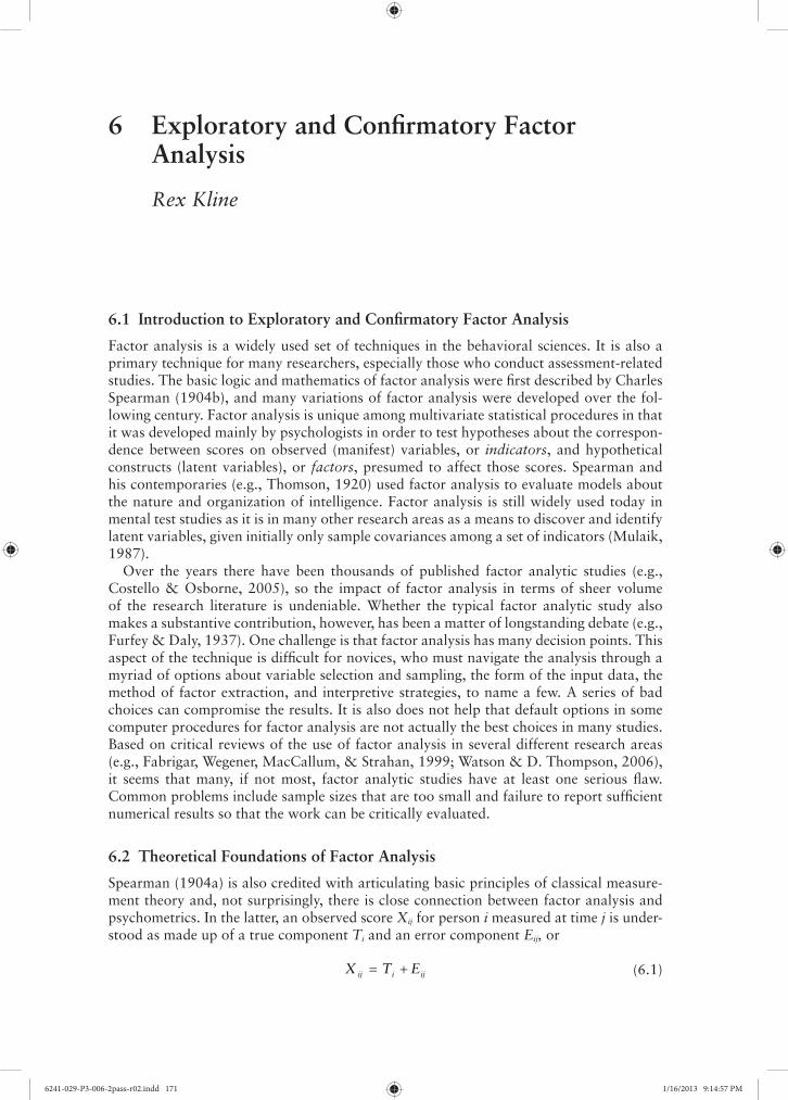
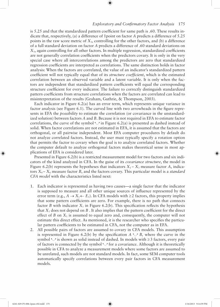
The proportion of total variance that is common is called communality, which is esti-mated by the statistic h2. For example, if h2 = .70, then 70% of total indicator variance is common and thus potentially explained by underlying factors. The rest, or 30% of the total variance, is unique variance, which is made up of specifi c variance (systematic but unshared) and measurement (random) error. Specifi c variance is not explained by com-mon factors; instead, it may be due to characteristics of individual indicators, such as the particular stimuli that make up a task, that also affect observed scores. The various parti-tions of standardized total indicator variance in factor analysis just described is illustrated in Figure 6.1.
Note in the fi gure that as the proportion of error variance increases, the proportion of systematic (true) variance decreases, which can in turn reduce the overall proportion of common variance. Statistical analysis of unreliable scores usually leads to inaccurate results, and factor analysis is no exception. In general, score reliabilities that exceed .90 are considered excellent, coeffi cients in the range of about .80 are considered good, but coeffi cients appreciably less than .70 are potentially problematic. If rXX < .50, then most
Figure 6.1 Basic partition of standardized indicator variance in factor analysis. h2, proportion of common variance, or communality; rXX , score reliability coeffi cient.
6241-029-P3-006-2pass-r02.indd 1726241-029-P3-006-2pass-r02.indd 172 1/16/2013 9:14:57 PM1/16/2013 9:14:57 PM
Exploratory and Confi rmatory Factor Analysis 173
of total variance is due to measurement error. Indicators with such low score reliabilities should be excluded from the analysis.
6.3 Kinds of Factor Analysis
There are two broad categories of factor analysis, exploratory (EFA) and confi rma-tory (CFA). Differences between these two techniques are listed next and then discussed afterward:
1. Unrestricted measurement models are estimated in EFA, but it is restricted measure-ment models that are analyzed in CFA. This means that the researcher must explicitly specify the indicator-factor correspondence in CFA, but there is no option to do so in EFA.
2. Unrestricted measurement models in EFA are not identifi ed, which means there is no unique set of statistical estimates for a particular model. This property concerns the rotation phase, which is part of most applications of EFA. In contrast, CFA models must be identifi ed before they can be analyzed, which means that there is only one exclusive set of estimates. Accordingly, there is no rotation phase in CFA.
3. It is assumed in EFA that the specifi c variance of each indicator is not shared with that of any other indicator. In contrast, CFA permits, depending on the model, estimation of whether specifi c variance is shared between pairs of indicators.
4. Output from CFA computer procedures contains the values of numerous fi t statistics that assess the fi t of the whole model to the data. In contrast, fi t statistics are not gen-erally available in standard methods of EFA (including principle components analysis and principle axis factoring, defi ned later) carried out by computer programs for gen-eral statistical analyses, such as SPSS (IBM, Corp, 2012) and SAS/STAT (SAS Institute, Inc., 2012), but some more specialized computer programs, such as Mplus (Muthén & Muthén, 1998–2012), may print certain types of fi t statistics for particular EFA methods.
5. Procedures for EFA are available in many computer tools for general statistical analy-ses, such as SPSS and SAS/STAT. In contrast, more specialized computer tools for structural equation modeling (SEM) are needed for CFA because the latter is the SEM technique for estimating restricted measurement models. Some widely used SEM com-puter tools include LISREL (Jöreskog & Sörbom, 2012) and Mplus (e.g., Kline, 2010, Chapter 4). The Mplus program has capabilities for both EFA and CFA.
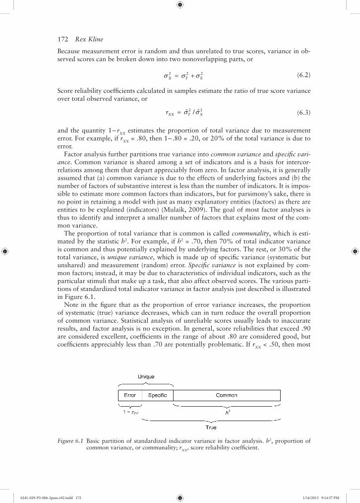
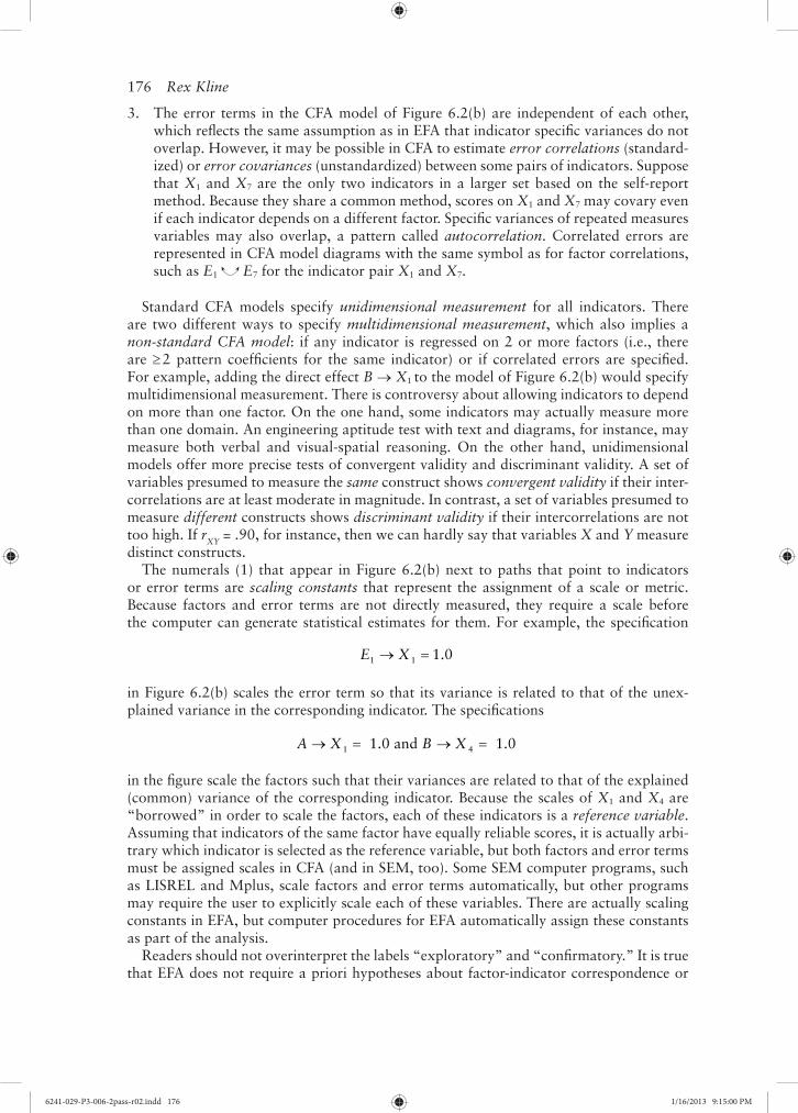
Presented in Figure 6.2 are two hypothetical measurement models for six indicators and two factors represented with symbols from SEM. These include squares or rectangles for observed variables, ellipses or circles for latent variables or error terms, lines with a single arrowhead (→) for presumed direct effects from causal variables to variables affected by them, two-headed curved arrows that exit and re-enter the same variable ( ) for vari-ances of factors or error terms; and curved line with two arrowheads ( ) for covariances (in the unstandardized solution) or correlations (in the standardized one) between either pairs of factors or pairs of error terms (Kline, 2010, chap. 5).
Depicted in Figure 6.2(a) is an unrestricted two-factor model of the kind analyzed in EFA. Without specifi c instruction from the user to do otherwise, an EFA computer proce-dure could theoretically generate all possible unrestricted factor solutions, which equals the number of indicators. The most basic solution is a single-factor model, which refl ects the assumption that all indicators depend on just one common factor. Next is a two-factor model, then a three-factor model, and so on up to the most complex model possible with just as many factors as indicators. In practice, EFA computer procedures rely on default
6241-029-P3-006-2pass-r02.indd 1736241-029-P3-006-2pass-r02.indd 173 1/16/2013 9:14:58 PM1/16/2013 9:14:58 PM
174 Rex Kline
statistical criteria for determining the number of factors to retain, but these defaults do not always correspond to best practice. These issues are elaborated later in the section about EFA, but the point now is that EFA does not require the researcher to specify the number of factors in advance.
The model in Figure 6.2(a) is unrestricted concerning the correspondence between in-dicators and factors. In EFA, each indicator is regressed on every factor in the model. The statistical estimates for this part of EFA are actually regression coeffi cients that may be in either standardized or unstandardized form, just as in the technique of multiple regres-sion. The difference is that predictors in ordinary regression are observed variables, but the predictors in EFA (and CFA, too) are latent variables. For example, there are two lines with single arrowheads that point to indicator X1 from each of the factors in Figure 6.2(a). These paths represent the presumed direct effects of both factors on X1, and the proper name of the statistical estimates of these effects is pattern coeffi cients. Many researchers refer to pattern coeffi cients as “factor loadings” or just “loadings,” but this term is inher-ently ambiguous for reasons explained later and thus is not used here. The larger point is that all possible pattern coeffi cients are calculated for each indicator in EFA.
Pattern coeffi cients in factor analysis are interpreted just as coeffi cients in standard mul-tiple regression.1 Suppose that the unstandardized pattern coeffi cient for the path A → X1
Figure 6.2 An exploratory factor analysis model and a confi rmatory factor analysis model for 6 indicators and 2 factors.
6241-029-P3-006-2pass-r02.indd 1746241-029-P3-006-2pass-r02.indd 174 1/16/2013 9:14:58 PM1/16/2013 9:14:58 PM
Exploratory and Confi rmatory Factor Analysis 175
is 5.25 and that the standardized pattern coeffi cient for same path is .60. These results in-dicate that, respectively, (a) a difference of 1point on factor A predicts a difference of 5.25 points in the raw score metric of X1, controlling for the other factors, and (b) a difference of a full standard deviation on factor A predicts a difference of .60 standard deviations on X1, again controlling for all other factors. In multiple regression, standardized coeffi cients are not generally correlation coeffi cients when the predictors covary. It is only in the very special case where all intercorrelations among the predictors are zero that standardized regression coeffi cients are interpreted as correlations. The same distinction holds in factor analysis: When the factors are correlated, the value of an indicator’s standardized pattern coeffi cient will not typically equal that of its structure coeffi cient, which is the estimated correlation between an observed variable and a latent variable. It is only when the fac-tors are independent that standardized pattern coeffi cients will equal the corresponding structure coeffi cient for every indicator. The failure to correctly distinguish standardized pattern coeffi cients from structure correlations when the factors are correlated can lead to misinterpretation of the results (Graham, Guthrie, & Thompson, 2003).
Each indicator in Figure 6.2(a) has an error term, which represents unique variance in factor analysis (see Figure 6.1). The curved line with two arrowheads in the fi gure repre-sents in EFA the possibility to estimate the correlation (or covariance in the unstandard-ized solution) between factors A and B. Because it is not required in EFA to estimate factor correlations, the curve of the symbol in Figure 6.2(a) is presented as dashed instead of solid. When factor correlations are not estimated in EFA, it is assumed that the factors are orthogonal, or all pairwise independent. Most EFA computer procedures by default do not analyze correlated factors. Instead, the user must typically specify a rotation option that permits the factor to covary when the goal is to analyze correlated factors. Whether the computer default to analyze orthogonal factors makes theoretical sense in most ap-plications of EFA is considered later.
Presented in Figure 6.2(b) is a restricted measurement model for two factors and six indi-cators of the kind analyzed in CFA. In the guise of its covariance structure, the model in Figure 6.2(b) represents the hypotheses that indicators X1 – X3 measure factor A, indica-tors X4 – X6 measure factor B, and the factors covary. This particular model is a standard CFA model with the characteristics listed next:
1. Each indicator is represented as having two causes—a single factor that the indicator is supposed to measure and all other unique sources of infl uence represented by the error term (e.g., A X1 E1). In CFA models with 2 factors, this property implies that some pattern coeffi cients are zero. For example, there is no path that connects factor B with indicator X1 in Figure 6.2(b). This specifi cation refl ects the hypothesis that X1 does not depend on B . It also implies that the pattern coeffi cient for the direct effect of B on X1 is assumed to equal zero and, consequently, the computer will not estimate this direct effect. As mentioned, it is the researcher who specifi es the particu-lar pattern coeffi cients to be estimated in CFA, not the computer as in EFA.
2. All possible pairs of factors are assumed to covary in CFA models. This assumption is represented in Figure 6.2(b) by the specifi cation A B, where the curve in the symbol is shown as solid instead of dashed. In models with 3 factors, every pair of factors is connected by the symbol for a covariance. Although it is theoretically possible in CFA to analyze a measurement models where some factors are assumed to be unrelated, such models are not standard models. In fact, some SEM computer tools automatically specify correlations between every pair factors in CFA measurement models.
6241-029-P3-006-2pass-r02.indd 1756241-029-P3-006-2pass-r02.indd 175 1/16/2013 9:14:59 PM1/16/2013 9:14:59 PM
176 Rex Kline
3. The error terms in the CFA model of Figure 6.2(b) are independent of each other, which refl ects the same assumption as in EFA that indicator specifi c variances do not overlap. However, it may be possible in CFA to estimate error correlations (standard-ized) or error covariances (unstandardized) between some pairs of indicators. Suppose that X1 and X7 are the only two indicators in a larger set based on the self-report method. Because they share a common method, scores on X1 and X7 may covary even if each indicator depends on a different factor. Specifi c variances of repeated measures variables may also overlap, a pattern called autocorrelation. Correlated errors are represented in CFA model diagrams with the same symbol as for factor correlations, such as E1 E7 for the indicator pair X1 and X7.
Standard CFA models specify unidimensional measurement for all indicators. There are two different ways to specify multidimensional measurement, which also implies a non-standard CFA model: if any indicator is regressed on 2 or more factors (i.e., there are 2 pattern coeffi cients for the same indicator) or if correlated errors are specifi ed. For example, adding the direct effect B X1 to the model of Figure 6.2(b) would specify multidimensional measurement. There is controversy about allowing indicators to depend on more than one factor. On the one hand, some indicators may actually measure more than one domain. An engineering aptitude test with text and diagrams, for instance, may measure both verbal and visual-spatial reasoning. On the other hand, unidimensional models offer more precise tests of convergent validity and discriminant validity. A set of variables presumed to measure the same construct shows convergent validity if their inter-correlations are at least moderate in magnitude. In contrast, a set of variables presumed to measure different constructs shows discriminant validity if their intercorrelations are not too high. If rXY = .90, for instance, then we can hardly say that variables X and Y measure distinct constructs.
The numerals (1) that appear in Figure 6.2(b) next to paths that point to indicators or error terms are scaling constants that represent the assignment of a scale or metric. Because factors and error terms are not directly measured, they require a scale before the computer can generate statistical estimates for them. For example, the specifi cation
1 1 1.0E X
in Figure 6.2(b) scales the error term so that its variance is related to that of the unex-plained variance in the corresponding indicator. The specifi cations
1 4 1.0 and 1.0A X B X
in the fi gure scale the factors such that their variances are related to that of the explained (common) variance of the corresponding indicator. Because the scales of X1 and X4 are “borrowed” in order to scale the factors, each of these indicators is a reference variable. Assuming that indicators of the same factor have equally reliable scores, it is actually arbi-trary which indicator is selected as the reference variable, but both factors and error terms must be assigned scales in CFA (and in SEM, too). Some SEM computer programs, such as LISREL and Mplus, scale factors and error terms automatically, but other programs may require the user to explicitly scale each of these variables. There are actually scaling constants in EFA, but computer procedures for EFA automatically assign these constants as part of the analysis.
Readers should not overinterpret the labels “exploratory” and “confi rmatory.” It is true that EFA does not require a priori hypotheses about factor-indicator correspondence or
6241-029-P3-006-2pass-r02.indd 1766241-029-P3-006-2pass-r02.indd 176 1/16/2013 9:15:00 PM1/16/2013 9:15:00 PM
Exploratory and Confi rmatory Factor Analysis 177
even the number of factors. However, there are ways to conduct EFA in a more confi rma-tory mode, such as instructing the computer to extract a certain number of factors based on theory. Also, the technique of CFA is not strictly confi rmatory. Specifi cally, it happens in perhaps most analyses that the initial restricted measurement model does not fi t the data. In this case, the researcher typically modifi es the hypotheses on which the initial model was based and specifi es a revised model. The respecifi ed model is then tested again with the same data. The goal of this process is to “discover” a model with three proper-ties: It makes theoretical sense, it is reasonably parsimonious, and its correspondence to the data is acceptably close.
This is a good point to mention two critical issues in factor analysis. One is the fac-tor indeterminacy problem, which is that hypothetical constructs can basically never be uniquely determined by their indicators. This means that although the results of a factor analysis might indicate that a particular measurement model is consistent with observed covariances, there may be nevertheless be other factor structures just as consistent with the same data. A more modern expression of the same idea refers to the problem of equivalent models, and for measurement models with multiple factors there are actually infi nitely many equivalent versions. This is not a fatal fl aw of factor analysis but instead a charac-teristic of statistical modeling in general. As noted by Mulaik (1987), such techniques are best seen as hypothesis-generating methods that support inductive reasoning but do not produce defi nitive, incontrovertible results. The second critical issue concerns the naming fallacy, or the false belief that the name assigned to a factor by a researcher means that the hypothetical construct is understood or even correctly labeled. Factor names are descrip-tions, not explanations, so we cannot assume that a particular factor label is necessarily the correct one. An example where the same two factors are assigned different labels by different researchers is presented later, but factor labels should be considered as hypoth-eses and not as substitutes for critical thinking.
6.4 Decision Points in Factor Analysis
Listed next are the basic decision points in factor analysis:
1. Whether factor analysis is the appropriate technique and, if so, whether to use EFA or CFA
2. The set of indicators to be analyzed and the composition and size (N) of the sample3. The data matrix to be analyzed; the basic choice is between a correlation matrix ver-
sus a covariance matrix
6.4.1 When Factor Analysis is Appropriate
The decision whether to conduct a factor analysis is usually not complicated. This is be-cause the technique’s basic purpose— description of latent variables that explain observed correlations—is pretty straightforward. Differences between EFA and CFA were consid-ered in the previous section. The technique of EFA may be a better choice in less mature research areas where basic measurement questions are not yet resolved. It also requires fewer a priori assumptions than CFA, which tests stronger hypotheses than EFA. In as-sessment research, EFA tends to be used in earlier studies and CFA in later studies in the same area. The selection of EFA or CFA implies additional decision point specifi c to each technique that are explained later in this chapter. Considered next are decisions that apply to both EFA and CFA.
6241-029-P3-006-2pass-r02.indd 1776241-029-P3-006-2pass-r02.indd 177 1/16/2013 9:15:00 PM1/16/2013 9:15:00 PM
178 Rex Kline
6.4.2 Indicator Selection
The selection of indicators is critical because the quality of what comes out of a fac-tor analysis (the results) depends heavily on the nature and quality of scores analyzed. Summarized next are recommendations by Fabrigar et al. (1999) concerning indicator selection: First, the researcher must defi ne the hypothetical constructs of interest. For ex-ample, if the goal is to delineate dimensions of anxiety, then the researcher should consult relevant theoretical and empirical works about the nature and number of factors, such as state anxiety, trait anxiety, anticipatory anxiety, social anxiety, and so on. Next, candidate indicators that as a set adequately sample the different domains should be identifi ed. Ide-ally, not all indicators will rely on the same method of measurement, such as assessment of anxiety through self-report questionnaires only. This is because common method vari-ance can affect all scores regardless of common latent variables. For instance, it is frequent in anxiety studies to measure physiological variables, such as heart rate or galvanic skin response, in addition to self-report.
It is also generally necessary to select multiple indicators of each presumed dimension. Multiple-indicator measurement not only tends to sample more facets of constructs of interest, but technical problems in the analysis are more likely to happen if some factors have too few indicators. This is especially true in small samples where some factors have just 2 indicators. In general, there should at least 3–5 indicators for each anticipated fac-tor. If a total of four anxiety dimensions are expected, for instance, then the minimum number of indicators would about 12–20 . But sometimes there are few theoretical or empirical bases for predicting the number of factors before conducting the analysis. In this case, the researcher must nevertheless try to delineate the population of indicators and then measure as many as possible in a suffi ciently large sample (Fabrigar et al., 1999). It is also crucial to select indicators with good psychometric characteristics.
As in most behavioral science studies, the sample should be representative of the popu-lation to which the results should generalize. For factor analysis, the sample should also be (a) relatively heterogeneous on the indicators but (b) relatively homogenous on other variables that do not covary substantially with the indicators (Mulaik, 2009). Because fac-tor analysis is essentially a regression technique where the predictors are latent variables, its results can be distorted by range restriction. Suppose that a researcher administers cog-nitive and scholastic ability tests within a sample of school children enrolled in programs for the gifted. Because the range of individual differences among gifted children on these may be relatively narrow, absolute magnitudes of intercorrelations among the tests may be restricted compared with a general sample of students. Because correlation is the “fuel” of factor analysis, results in range-restricted samples may not be very meaningful. However, relative homogeneity among participants on other variables, such as demographic char-acteristics, that are not strongly related to the indicators helps to ensure that the factors affect scores of all cases the same way. That is, the same basic measurement model should hold for all cases (Mulaik, 2009).
6.4.3 Sample Size
A critical question concerns minimum sample sizes required for the analysis. In general, factor analysis is a large sample technique, so the more cases the better. (This assumes that a larger sample is just as representative as a smaller one.) Early sample size recommenda-tions for EFA were based on ratios of the number of cases to the number of indicators. For example, the recommendation for a 10:1 ratio means that there are at least 10 cases for every indicator, so an analysis of 10 indicators would require a minimum sample size of
6241-029-P3-006-2pass-r02.indd 1786241-029-P3-006-2pass-r02.indd 178 1/16/2013 9:15:00 PM1/16/2013 9:15:00 PM

Exploratory and Confi rmatory Factor Analysis 179
100; a more stringent 20:1 ratio would require at least N = 200 for 10 indicators, and so on. There are two problems with such guidelines. First, there is no clear consensus in the literature about the optimal cases-to-indicators ratios for EFA. A 10:1 ratio is probably the most common guideline, but some methodologists advocate even higher ratios, such as 20:1. Second, sample size requirements depend on the population (true) factor model. pecifi cally, fewer cases are needed when each factor has at least 3–4 indicators and average communalities across the indicators are about .70 or higher (e.g., MacCallum, Widaman, Zhang, & Hong, 1999). In this ideal scenario, a 10:1 cases-to-indicators ratio may suffi ce, but absolute sample sizes less than 100 may be untenable in factor analysis. A minimum sample size of 200 seems more defensible. However, cases-to-indicators ratios that exceed 20:1 and minimum sample sizes of 400 or more may be required when the ideal conditions just listed do not hold (Fabrigar et al., 1999).
Results of some reviews suggest that sample sizes in published EFA studies are typically too small. For example, Costello and Osborne (2005) surveyed a total of 305 factor ana-lytic studies published over a two-year period and listed in the PsychINFO database. Most of these analyses (63%) were conducted with cases-to-indicators ratios <10:1, and a total of 41% were based on ratios < 5:1. Only 21% of the studies featured cases-to-indicators ratios > 20:1. In a separate computer simulation study where factor analyses were con-ducted in generated samples of different sizes, Costello and Osborne (2005) found that most factor solutions based on cases-to-indicators ratios <10:1 were incorrect. When the ratio is 2:1, however, the rate of incorrect results was 90%, and almost one-third of these analyses failed due to technical problems.
Ratio-type recommendations for minimum sample sizes in CFA are not based on the number of indicators but instead on the number of parameters in the entire measurement model. In CFA, parameters include pattern coeffi cients, error variances and covariances (i.e., for correlated errors), and factor variances and covariances. Models with more param-eters—even for the same number of indicators—require more estimates, so larger samples are necessary in order for the results to be reasonably precise. Sample size requirements in CFA also vary with the type of estimation method used and the distributional characteristics of the data. In general, somewhat smaller sample sizes are needed when the standard esti-mation method in SEM, maximum likelihood (ML) estimation, is used and the distributions are multivariate normal. In this case, a 20:1 ratio is recommended, that is, there should be at least 20 cases for each model parameter estimated in the analysis (e.g., Jackson, 2003). A “typical” sample size in SEM is about 200 (e.g., Shah & Goldstein (2006), which may be adequate for analyzing a CFA model with 10 or so parameters. However, much larger sam-ple sizes may be needed when a method other than ML estimation is used or distributions are severely non-normal. Another framework for estimating minimum sample sizes in CFA involves estimation of the statistical power of tests about either individual parameters or about the fi t of the whole model to the data. A variation is to specify a target level of power, such as .80, and then estimate the minimum sample size needed for that target—see Mac-Callum, Browne, and Sugawara (1996) and Kline (2010, chapter 8) for more information.
6.5 Data Matrix Analyzed
Most researchers input raw data fi les for computer statistical analyses. These same re-searchers may be surprised to learn that the raw data themselves are not necessary for most types of factor analysis. Specifi cally, if a raw data fi le is submitted, the computer will create its own matrix summary of the data, which is then analyzed. It is also possible in many computer tools to input a matrix summary instead of raw data. The capability to analyze summary statistics also provides the basis for a secondary analysis in which data
6241-029-P3-006-2pass-r02.indd 1796241-029-P3-006-2pass-r02.indd 179 1/16/2013 9:15:00 PM1/16/2013 9:15:00 PM
180 Rex Kline
collected by others are reanalyzed but where the raw data are unavailable. Many journal articles about the results of factor analysis contain enough information, such as correla-tions and standard deviations, to create a matrix summary of the data, which can then be submitted to a computer program for analysis. Thus, readers of these works can, with no access to the raw data, replicate the original analyses or estimate alternative models not considered in the original work. This is why it is best practice for researchers to report suffi cient summary statistics for a future secondary analysis.
There are two basic types of matrix summaries of raw data, a Pearson correlation (r) matrix and a covariance (cov) matrix. The default matrix analyzed in most EFA computer procedures is a correlation matrix. Pearson correlations measure the degree of linear as-sociation between two continuous variables. Specifi cally, r measures the degree to which the rank order of scores on one variable corresponds to the rank order on the other vari-able also taking account of the relative distances between the scores. The entries in the diagonal of a correlation matrix all equal 1.0, which are also the variances of all variables in a standardized metric.
The default data matrix in SEM computer programs is the covariance matrix. This is because the standard method in SEM, ML estimation, analyzes unstandardized variables. It is possible in SEM to fi t a CFA model to a correlation matrix, but special methods are needed (Kline, 2010, chapter 7). The diagonal entries in a covariance matrix are the vari-ances of the indicators in their original (unstandardized) metrics. The off-diagonal entries are the covariances, which for two continuous variables X and Y is
X Ycov r SD SD (6.4)
where r is the Pearson correlation and SDX and SDY are their standard deviations. A co-variance thus represents the strength of the association between X and Y and their vari-abilities, albeit with a single number. Because the covariance is an unstandardized statistic, its value has no upper or lower bound. For example, covariances of, say, –1,003.26 or 13.58 are possible. The statistic cov encapsulates all the information measured by r plus the degree of “spreadoutedness” of the scores on both indicators (B. Thompson, 2004).
Because the information conveyed by cov and r is not the same, it can happen that the fi t of a measurement model to a correlation matrix is not the same as the fi t of the same model to a covariance matrix in the same sample. Also, the factor analysis of a covariance matrix generates two sets of estimates, an unstandardized solution and a standardized solution. Only the latter is calculated by the computer when a correlation matrix is ana-lyzed. For all these reasons, think carefully about the choice of which type of data matrix to analyze and report that choice in written summaries of the results. Finally, the analysis of correlations or covariances assumes that the indicators are continuous variables. This is most likely to be true when each indicator is a scale that generates a total score over a set of items. However, individual items with Likert-type response formats (e.g., 0 = disagree, 1 = uncertain, 2 = agree) are not continuous variables. Instead, they are generally consid-ered to be ordinal, and their distributions tend to be non-normal. Therefore, analyzing a Pearson correlation matrix (or the corresponding covariance matrix) when the indicators are items may not be appropriate. The analysis of items in factor analysis is considered later in this chapter; the discussion that follows assume the analysis of scales.
6.6 Exploratory Factor Analysis
Summarized next is the typical sequence of additional decisions in EFA. These steps are sometimes iterative because results at a later phase may necessitate a return to an earlier step:
6241-029-P3-006-2pass-r02.indd 1806241-029-P3-006-2pass-r02.indd 180 1/16/2013 9:15:00 PM1/16/2013 9:15:00 PM

Exploratory and Confi rmatory Factor Analysis 181
1 Select a method of factor extraction. The most basic choice is between principal axes factoring (PAF)—also known as common factor analysis—and principal components analysis (PCA). The PCA method is the default in some EFA computer procedures, such as SPSS, but this option is not always the best.
2 Decide how many factors to retain. There are two kinds of criteria for making this choice, theoretical and statistical. Of the two, theoretical criteria may result in less capitalization on sample-specifi c (chance) variation than statistical criteria.
3 Select a rotation method and interpret the factors. The goal of rotation is to enhance the interpretability of the retained factors. There are many different rotation methods, but the most basic choice is between some type of orthogonal rotation where the factors are independent or oblique rotation where the factors are allowed to covary. The default method in most EFA computer procedures is orthogonal rotation, but this option is not always ideal.
6.6.1 Factor Extraction Method
The difference between PAF and PCA—and the only difference—is the form of the data matrix analyzed (B. Thompson, 2004). The PCA method assumes that all indicator vari-ance is common (shared) variance. The assumption is strict because it does not allow for specifi c variance or measurement error (see Figure 6.1); that is, the method assumes that the scores are perfectly reliable. Accordingly, all observed variance is analyzed in PCA. This means that the correlation matrix analyzed by PCA has diagonal entries that all equal 1.0, which is literally all the observed variance in standardized form. The data matrix ana-lyzed in PCA is thus called an unreduced correlation matrix. In contrast, the PAF method analyzes common variance only. This means that the diagonal entries of 1.0 in the correla-tion matrix are replaced in the PAF method by h2 statistics, or estimated communalities for each indicator. Suppose that the estimated communality for indicator X3 is .75. In the correlation matrix, the 1.0 in the diagonal entry for X3 will be replaced by .75 in PAF. All remaining diagonal entries of 1.0 are also replaced by the corresponding h2 value for each of the other indicators, and in each case h2 1.0. Thus, it is a reduced correlation matrix that is analyzed in PAF. When a covariance matrix is analyzed, the diagonal entries in PAF are replaced by the product of the sample variance and the communality estimate for each indicator. Because the PAF method analyzes common variance, it does not assume perfect score reliability.
Statistical procedures for PAF typically use an iterative method to estimate commu-nalities where the computer derives initial estimates and then attempts to improve these estimates through subsequent cycles of calculations. The default initial estimate for each indicator is usually the squared multiple correlation (SMC) between that indicator and all rest. For example, if SMC = .60 for indicator X4, then 60% of the observed variance in X4 is explained by all the other indicators. However, sample correlations (and squared correlations, too) can be attenuated by measurement error, and iterative estimation takes account of this phenomenon. Sometimes in PAF it happens that iterative estimation fails, that is, the computer is unable to derive a fi nal set of communality estimates. Iteration failure may be indicated by a warning or error message in the output. Any subsequent es-timates in the rest of the output should be ignored. Another sign of trouble are Heywood cases, or estimates that are mathematically impossible, such as a structure coeffi cient >1.0 or a negative (<0) estimate of error variance. Solutions with Heywood cases are inadmis-sible and warrant no further interpretation. Some PAF computer procedures allow the user to increase the default limit on the number of iterations, which gives the computer more “tries” and may solve the problem. Some programs also accept user-specifi ed initial
6241-029-P3-006-2pass-r02.indd 1816241-029-P3-006-2pass-r02.indd 181 1/16/2013 9:15:00 PM1/16/2013 9:15:00 PM
182 Rex Kline
communality estimates that replace the default initial estimate. Failure of iterative estima-tion is more likely in small samples, when score reliabilities are low, or there are too few indicators of some factors. Communalities are not estimated in PCA, so the potential problems of iteration failure and Heywood cases are not encountered in this method.
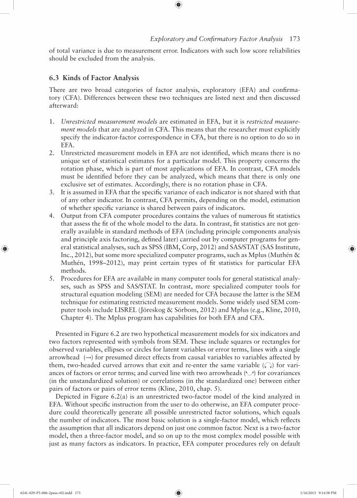
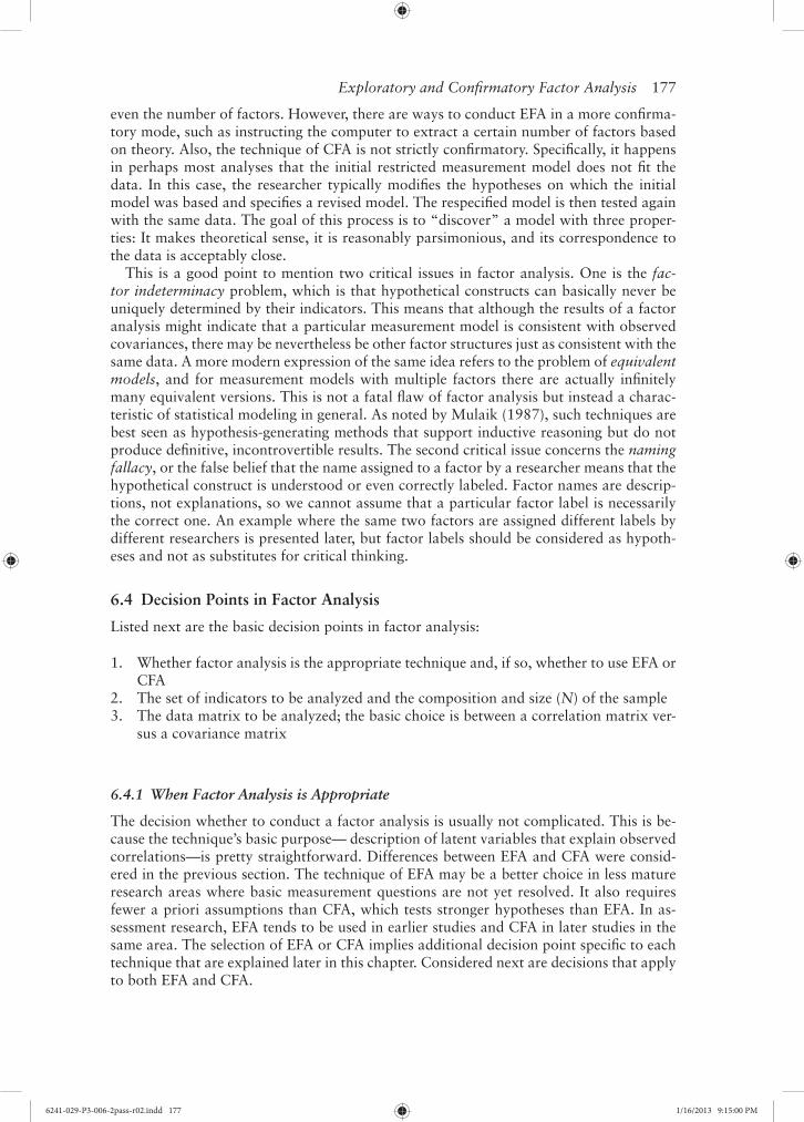
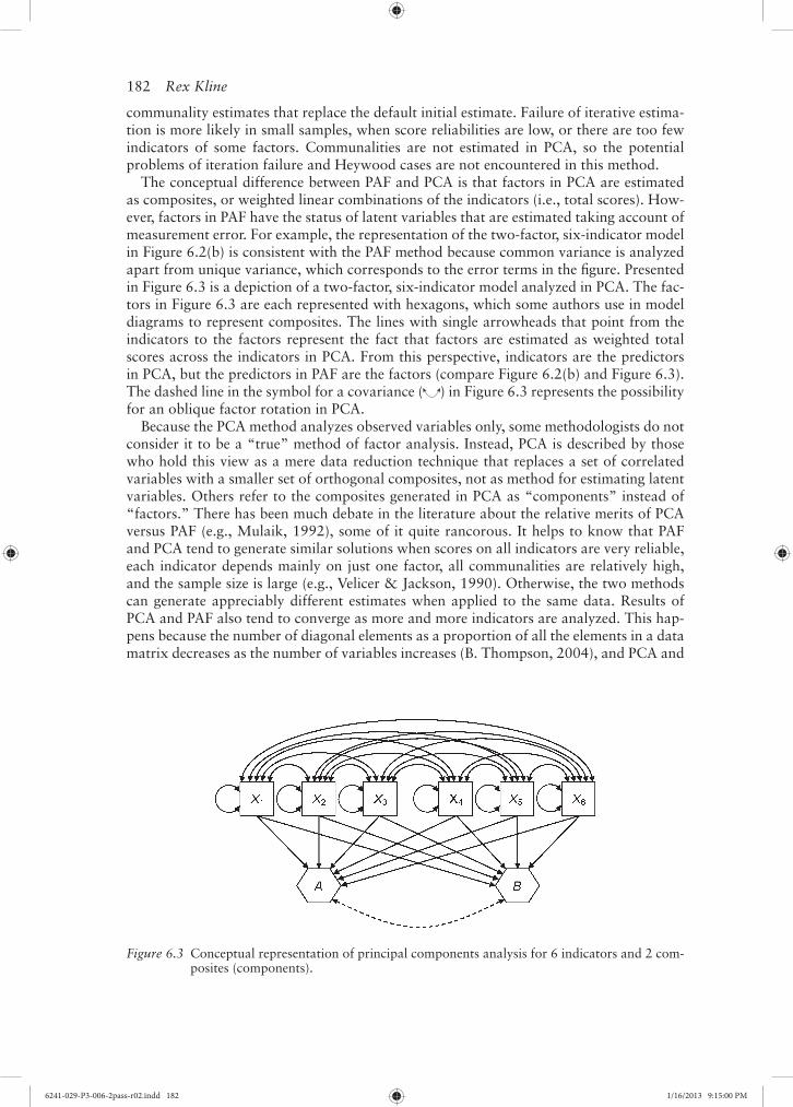
The conceptual difference between PAF and PCA is that factors in PCA are estimated as composites, or weighted linear combinations of the indicators (i.e., total scores). How-ever, factors in PAF have the status of latent variables that are estimated taking account of measurement error. For example, the representation of the two-factor, six-indicator model in Figure 6.2(b) is consistent with the PAF method because common variance is analyzed apart from unique variance, which corresponds to the error terms in the fi gure. Presented in Figure 6.3 is a depiction of a two-factor, six-indicator model analyzed in PCA. The fac-tors in Figure 6.3 are each represented with hexagons, which some authors use in model diagrams to represent composites. The lines with single arrowheads that point from the indicators to the factors represent the fact that factors are estimated as weighted total scores across the indicators in PCA. From this perspective, indicators are the predictors in PCA, but the predictors in PAF are the factors (compare Figure 6.2(b) and Figure 6.3). The dashed line in the symbol for a covariance ( ) in Figure 6.3 represents the possibility for an oblique factor rotation in PCA.
Because the PCA method analyzes observed variables only, some methodologists do not consider it to be a “true” method of factor analysis. Instead, PCA is described by those who hold this view as a mere data reduction technique that replaces a set of correlated variables with a smaller set of orthogonal composites, not as method for estimating latent variables. Others refer to the composites generated in PCA as “components” instead of “factors.” There has been much debate in the literature about the relative merits of PCA versus PAF (e.g., Mulaik, 1992), some of it quite rancorous. It helps to know that PAF and PCA tend to generate similar solutions when scores on all indicators are very reliable, each indicator depends mainly on just one factor, all communalities are relatively high, and the sample size is large (e.g., Velicer & Jackson, 1990). Otherwise, the two methods can generate appreciably different estimates when applied to the same data. Results of PCA and PAF also tend to converge as more and more indicators are analyzed. This hap-pens because the number of diagonal elements as a proportion of all the elements in a data matrix decreases as the number of variables increases (B. Thompson, 2004), and PCA and
Figure 6.3 Conceptual representation of principal components analysis for 6 indicators and 2 com-posites (components).
6241-029-P3-006-2pass-r02.indd 1826241-029-P3-006-2pass-r02.indd 182 1/16/2013 9:15:00 PM1/16/2013 9:15:00 PM
Exploratory and Confi rmatory Factor Analysis 183
PAF analyze the same data matrix except for the diagonal entries. In SPSS, the initial fac-tor solution is extracted using PCA even if the user requested PAF extraction for the fi nal solution. In general, PAF is a better choice than PCA when not all score reliabilities are high (e.g., rXX > .80).
Some other EFA extraction methods are briefl y described next; see Mulaik (2009, chap-ter 7) for more information. The method of alpha factor analysis is a generalization of the internal consistency reliability coeffi cient (i.e., Cronbach’s alpha) but in this case applied to indicators of different factors instead of to items within the same test. This method associates indicators with factors in a way that maximizes the internal consistency of construct measurement. The method of image analysis minimizes the chance that a factor will be defi ned mainly by a single indicator. This outcome is undesirable in factor analy-sis because single-indicator measurement is generally imprecise compared with multiple-indicator measurement. Image analysis works by minimizing the effect of specifi c variance on the results. In maximum likelihood factor analysis, the method of ML estimation is used to derive common factors that reproduce sample correlations among the indicators as close as possible. The method also generates statistical tests of parameter estimates, including the pattern coeffi cients and factor correlations. In contrast, these kinds of sta-tistical tests are not available in the PAF and PCA methods. In SPSS, the ML method is applied to correlation matrices only.
6.6.2 Number of Retained Factors
Sometimes the decision about the number of factors to retain is determined by theory, such as when a cognitive ability test battery is constructed in order to assess three different underlying domains. In this case, it makes sense to specify a three-factor solution. Even when theory indicates a specifi c number of factors, many researchers will nevertheless inspect a range of factor solutions, such as solutions with two, three, or four factors for the example just mentioned. Doing so not only evaluates the original hypothesis about the presence of three factors; it also allows for alternative explanations (i.e., two or four factors) to be tested. There are also various statistical criteria for determining the number of retained factors. It is best not to blindly apply these criteria because doing so tends to capitalize on chance variation in a particular sample. Instead, a researcher should inspect statistical criteria in light of extant theory.
This fi rst statistical criterion is the default basis in most EFA computer procedures for determining the number of retained factors, but this method is not always the best choice. It is the eigenvalue >1.0 rule, also known as the Kaiser criterion or K1 rule after the edu-cational statistician Henry F. Kaiser. Every extracted factor in EFA has its own eigenvalue, which is a measure of the proportion of variance in the indicators explained by that factor and is designated by the symbol λ. The fi rst extracted factor tends to have the highest ei-genvalue, and eigenvalues tend to successively decrease as additional factors are extracted. An eigenvalue is the sum of the squared structure coeffi cients across all the indicators. If λ = 1.0, then the amount of variance explained by that factor corresponds to the amount of information in one indicator, and if λ = 2.0, the explanatory power corresponds to the vari-ability of two indicators, and so. The ratio λ/nj where ni is the number of indicators is the proportion of total variance explained by the associated factor. The sum of the eigenvalues for all possible factors equals the number of indicators, and the ratio of the sum of the eigenvalues across all retained factors divided by the number of indicators is the total pro-portion of variance explained by the factors as a set (B. Thompson, 2004). These propor-tions of explained variance are another type of variance-accounted-for effect size in EFA. The λ 1.0 rule thus requires that a factor explains at least one “unit” of information in
6241-029-P3-006-2pass-r02.indd 1836241-029-P3-006-2pass-r02.indd 183 1/16/2013 9:15:01 PM1/16/2013 9:15:01 PM
184 Rex Kline
terms of the indicators. However, note that the λ 1.0 rule applies to factors extracted using the PCA method, not the PAF method. Indeed, it is a mistake to apply this rule when a reduced correlation or covariance matrix is analyzed (Fabrigar et al., 1999).
There are two problems with blindly following the λ 1.0 rule. First, sampling error af-fects the estimation of eigenvalues, which ignores that the fact that λ 1.01 versus λ .99 leads to categorically different outcomes (i.e., retain vs. do not retain) under this rule. Sec-ond, factor solutions determined by the λ 1.0 rule tend to have too many factors but also occasionally too few factors (e.g., Velicer & Jackson, 1990). In general, the λ 1.0 rule is not a sound basis for deciding how many factors to retain. A variation is the Cattell scree test (after the psychologist Raymond B. Cattell), which is a visual heuristic that involves making a line graph where eigenvalues are plotted on the Y-axis for each of the total pos-sible number of factors, which are represented on the X-axis. The graph is then visually inspected in order to locate the point where the drop in eigenvalues over successive fac-tors levels out and from which the slope of the line is basically horizontal. The number of retained factors in this approach corresponds to the number of eigenvalues before the last substantial drop in the graph. A drawback of the scree test is that its interpretation can be rather subjective in that two different researchers can come to different conclusions after inspecting the same plot.
A more sophisticated method based on eigenvalues is that of parallel analysis, which in-volves the comparison of observed eigenvalues against those expected from random data. One way to conduct a parallel analysis is to use a computer procedure to randomize the scores for each variable in a raw data fi le.2 The randomized scores have the same distribu-tional characteristics of the original scores, but their expected intercorrelations are about zero. Next, eigenvalues from the analysis of the randomized scores are compared against those from the original data. Factors are retained whenever the eigenvalues based on the original scores are greater than the eigenvalues for the corresponding factors based on the randomized scores. Suppose that the eigenvalues for the fi rst three factors based on ana-lyzing the original scores are, respectively, 5.525, 2.350, and 1.026. The corresponding eigenvalues based on the randomized scores are 2.770, 1.850, and 1.332. This pattern suggests that fi rst two factors should be retained but not the third because 1.332 (based on the randomized scores) is greater than 1.026 (based on the original scores). Results of computer simulation studies about parallel analysis have generally been favorable (e.g., Crawford et al., 2010), but Fabrigar et al. (1999) noted that the decision to retain factors can be rather arbitrary when the pair of eigenvalues for a particular factor are very similar.
Most researchers retain fewer factors than the number of indicators, and such solutions typically explain some proportion of the total variance of the indicators, but usually not all of it. This also means that the factors will not perfectly explain the sample correlations (i.e., the data). Many EFA computer procedures optionally print predicted correlations—also called reproduced correlations—and residual correlations. The former are the values of predicted Pearson correlations for the set of indicators, given the factor solution, and the latter are the differences between the observed and predicted correlations for each indica-tor. The lower the residuals in absolute value, the better the explanatory power of a factor solution. There is no absolute cut-off for interpreting residual correlations, but a better result is indicated if all absolute residuals are < .05. However, absolute residuals >.10 sug-gest poor prediction of the corresponding correlation.
It is generally better in EFA to extract too many factors, or overfactoring, than to retain too few, or underfactoring. This is because there tends to be substantial error in the results with under-factoring. For example, estimation of pattern coeffi cients of indicators that actually depend on a factor may complicate accurate estimation of coeffi cients of other in-dicators that measure retained factors. Two factors that are really distinct may be merged
6241-029-P3-006-2pass-r02.indd 1846241-029-P3-006-2pass-r02.indd 184 1/16/2013 9:15:01 PM1/16/2013 9:15:01 PM
Exploratory and Confi rmatory Factor Analysis 185
in a model with too few factors, which may complicate interpretation of the underlying latent variables (Fabrigar et al., 1999). Over-factoring is not without penalty, including the interpretation of factors that do really correspond to hypothetical constructs in the population. Overfactoring is also a potential drawback of the λ 1.0 rule.
6.6.3 Method of Rotation
The option for rotation does not apply when only a single factor is retained; otherwise, rotation is part of just about all analyses of multifactor models in EFA. The initial factor solution is often diffi cult to interpret. This is because the structure coeffi cients for the as-sociations between the fi rst factor and all indicators tend to uniformly high, and patterns of correlations with the remaining factors may not be very distinct. The goal of rotation is to make the meaning of the factors more obvious to the researcher. It works by reweight-ing the initial factors (i.e., the factor axes are shifted) according to statistical criteria that vary with the particular method of rotation. The desired outcome is a rotated solution that exhibits simple structure where each factor explains as much variance as possible in nonoverlapping sets of indicators. That is, the structure coeffi cients for the rotated factors should head toward either 0 or 1.0 in order to make the associations between factors and indicators more distinct. Theoretically, there are an infi nite number of possible factor rota-tions for a given solution. In practice, either the researcher specifi es a rotation option in a computer procedure for EFA or the computer will employ its default method.
There are two main classes of rotation methods in EFA. In orthogonal rotation, the rotated factors are all uncorrelated just as they are in the initial solution. Consequently, values of the standardized pattern coeffi cient and the structure coeffi cient for each indi-cator are equal. The most widely used rotation method of any kind is Kaiser’s varimax rotation, which is also the default in SPSS. Varimax rotation maximizes the variance of the structure coeffi cients (i.e., it pushes them toward 0 or 1.0) for each factor, which tends to (a) limit the number of indicators with high correlations with that factor and (b) evenly distribute the indicators across the factors. This method is used so often because it gener-ally yields simple structure in perhaps most EFA studies where the factors are uncorrelated (B. Thompson, 2004). A related method is quartimax rotation, which maximizes the vari-ance of the structure coeffi cients for each indicator. This tends to yield a factor solution with a general factor that correlates highly with most indicators and lesser factors each associated with different subsets of indicators. The method of equamax rotation offers a kind of “comprise” in that it maximizes a weighted function of the criteria from the vari-max method and the quartimax method. Selection among these alternatives for orthogo-nal rotation should be guided by the researcher’s hypotheses about the anticipated model.
The assumption of all orthogonal rotation methods is that the underlying constructs are uncorrelated, but this hypothesis is not always defensible (Fabrigar et al., 1999). For ex-ample, it makes little sense that various latent cognitive abilities, such as verbal reasoning, visual-spatial reasoning, and memory, would be unrelated to each other. It seems just as implausible to presume that certain latent affective domains, such as anxiety and depres-sion, are independent. Methods of oblique rotation allow the factors to covary; that is, they estimate measurement models with correlated factors. Note that the specifi cation of oblique rotation does not somehow “force” the factors to covary. Instead, these methods estimate factor correlations, given the data, so these estimates are “allowed” to be close to zero, if such estimates are consistent with the data. However, if an estimated factor correlation is extremely high (e.g., ), then the two factors are clearly not distinct (i.e., there are too many factors). Also, the pattern coeffi cients and the structure coeffi cient for the same indicator are typically unequal when the factors covary.
6241-029-P3-006-2pass-r02.indd 1856241-029-P3-006-2pass-r02.indd 185 1/16/2013 9:15:01 PM1/16/2013 9:15:01 PM
186 Rex Kline
Promax rotation is probably the most widely used oblique rotation method. It usually begins with a varimax-rotated solution and then raises the pattern coeffi cients to a higher power κ (kappa), which tends to force near-zero coeffi cients to approach zero faster than coeffi cients further from zero (Mulaik, 2009). The procedure then generates least squares estimates of the target matrix just described by allowing the factors to covary. A param-eter of promax rotation is κ, or the power to which coeffi cients in the target matrix are raised. Values of κ usually range from 1 through 4, where higher values permit higher absolute estimates of factor correlations that are consistent with data. The default in SPSS is κ = 4, and it is usually unnecessary to change this value. Another oblique method is direct oblimin rotation, which is a member of a family of oblimin methods that generally minimize the variance of the pattern coeffi cients across different factors while estimating factor correlations. The parameter for direct oblimin rotation in SPSS is referred to as δ (delta), which ranges from negative to positive in value up to a maximum of .80 (i.e., δ .80). Lower values of δ tend to decrease absolute estimates of factor correlations and higher values result in just the opposite. The default in SPSS is δ 0, and is rarely necessary to specify a different value.
A potential drawback of oblique rotation is that interpretation of the factors may be more diffi cult. One reason is that there are two sets of standardized coeffi cients, pattern and structure, and it can happen that and their values for the same indicator are quite different. For example, if an indicator’s structure coeffi cient is about zero but its pattern coeffi cient is not, then a suppression effect is indicated. This means that the indicator contributes to the factor indirectly by changing the relations of other indictors to the same factor (B. Thompson, 2004). Another sign of suppression is when the signs of the pattern coeffi cient and structure coeffi cients for the same indicator are different. A second compli-cation of oblique rotation is that there are few guidelines for applied researchers concern-ing the specifi cation of values of parameters for the promax and oblimin methods other than the default values that would be suitable for a particular set of indicators (Costello & Osborne, 2005).
There are many other rotation methods in EFA, and it can be diffi cult to decide which method is best. There is also some degree of trial and error in their use. For example, it could happen in a particular analysis that a promax oblique rotation generates results that are easier to interpret than an oblimin oblique rotation. However, if the results are dramatically different after application of different rotation methods, then there may be little basis to pick one solution or the other when no replication sample is available. How-ever, a robust underlying measurement model with simple structure assessed with psycho-metrically sound indicators should be detected by different rotation methods. See Mulaik (2009, Chapters 10–12) for more information about factor rotation in EFA.
6.6.4 Empirical Example
The fi rst edition of the Kaufman Assessment Battery for Children (KABC-I; Kaufman & Kaufman, 1983) is an individually-administered cognitive ability test for children ages 2½–12½ years old. The test’s authors claimed that the KABC -I’s eight subtests measure two factors. The three tasks believed to refl ect sequential processing all require the correct recall of auditory stimuli (Number Recall, Word Order) or visual stimuli (Hand Move-ments) in a particular order. The other fi ve tasks—Gestalt Closure, Triangles, Spatial Memory, Matrix Analogies, and Photo Series—are supposed to measure more holistic, less order-dependent reasoning, or simultaneous processing. Each of these tasks requires that the child grasps a gestalt but with somewhat different formats and stimuli that all
6241-029-P3-006-2pass-r02.indd 1866241-029-P3-006-2pass-r02.indd 186 1/16/2013 9:15:01 PM1/16/2013 9:15:01 PM
Exploratory and Confi rmatory Factor Analysis 187
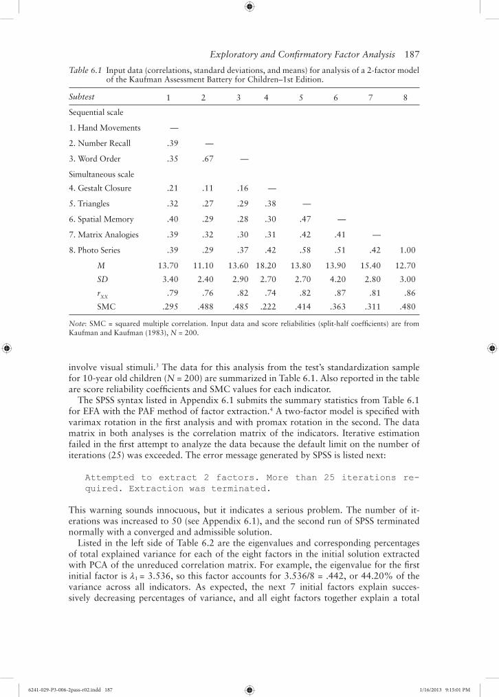
Table 6.1 Input data (correlations, standard deviations, and means) for analysis of a 2-factor model of the Kaufman Assessment Battery for Children–1st Edition.
Subtest 1 2 3 4 5 6 7 8
Sequential scale
1. Hand Movements —
2. Number Recall .39 —
3. Word Order .35 .67 —
Simultaneous scale
4. Gestalt Closure .21 .11 .16 —
5. Triangles .32 .27 .29 .38 —
6. Spatial Memory .40 .29 .28 .30 .47 —
7. Matrix Analogies .39 .32 .30 .31 .42 .41 —
8. Photo Series .39 .29 .37 .42 .58 .51 .42 1.00
M 13.70 11.10 13.60 18.20 13.80 13.90 15.40 12.70
SD 3.40 2.40 2.90 2.70 2.70 4.20 2.80 3.00
rXX .79 .76 .82 .74 .82 .87 .81 .86
SMC .295 .488 .485 .222 .414 .363 .311 .480
Note: SMC = squared multiple correlation. Input data and score reliabilities (split-half coeffi cients) are from Kaufman and Kaufman (1983), N = 200.
involve visual stimuli.3 The data for this analysis from the test’s standardization sample for 10-year old children (N = 200) are summarized in Table 6.1. Also reported in the table are score reliability coeffi cients and SMC values for each indicator.
The SPSS syntax listed in Appendix 6.1 submits the summary statistics from Table 6.1 for EFA with the PAF method of factor extraction.4 A two-factor model is specifi ed with varimax rotation in the fi rst analysis and with promax rotation in the second. The data matrix in both analyses is the correlation matrix of the indicators. Iterative estimation failed in the fi rst attempt to analyze the data because the default limit on the number of iterations (25) was exceeded. The error message generated by SPSS is listed next:
Attempted to extract 2 factors. More than 25 iterations re-quired. Extraction was terminated.
This warning sounds innocuous, but it indicates a serious problem. The number of it-erations was increased to 50 (see Appendix 6.1), and the second run of SPSS terminated normally with a converged and admissible solution.
Listed in the left side of Table 6.2 are the eigenvalues and corresponding percentages of total explained variance for each of the eight factors in the initial solution extracted with PCA of the unreduced correlation matrix. For example, the eigenvalue for the fi rst initial factor is λ1 = 3.536, so this factor accounts for 3.536/8 = .442, or 44.20% of the variance across all indicators. As expected, the next 7 initial factors explain succes-sively decreasing percentages of variance, and all eight factors together explain a total
6241-029-P3-006-2pass-r02.indd 1876241-029-P3-006-2pass-r02.indd 187 1/16/2013 9:15:01 PM1/16/2013 9:15:01 PM
188 Rex Kline
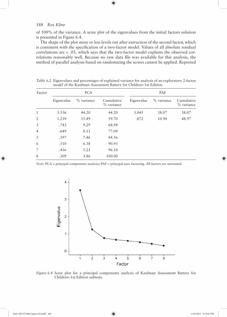
Table 6.2 Eigenvalues and percentages of explained variance for analysis of an exploratory 2-factor model of the Kaufman Assessment Battery for Children–1st Edition.
Factor PCA PAF
Eigenvalue % variance Cumulative % variance
Eigenvalue % variance Cumulative % variance
1 3.536 44.20 44.20 3.045 38.07 38.07
2 1.239 15.49 59.70 .872 10.90 48.97
3 .743 9.29 68.98
4 .649 8.11 77.09
5 .597 7.46 84.56
6 .510 6.38 90.93
7 .416 5.21 96.14
8 .309 3.86 100.00
Note. PCA = principal components analysis; PAF = principal axes factoring. All factors are unrotated.
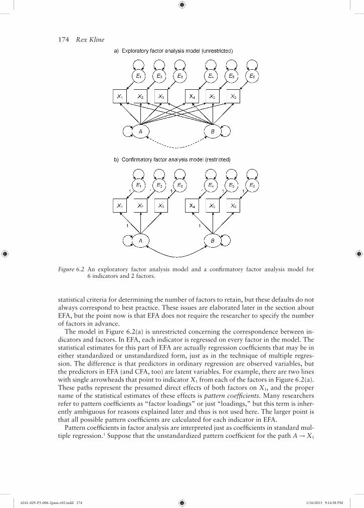
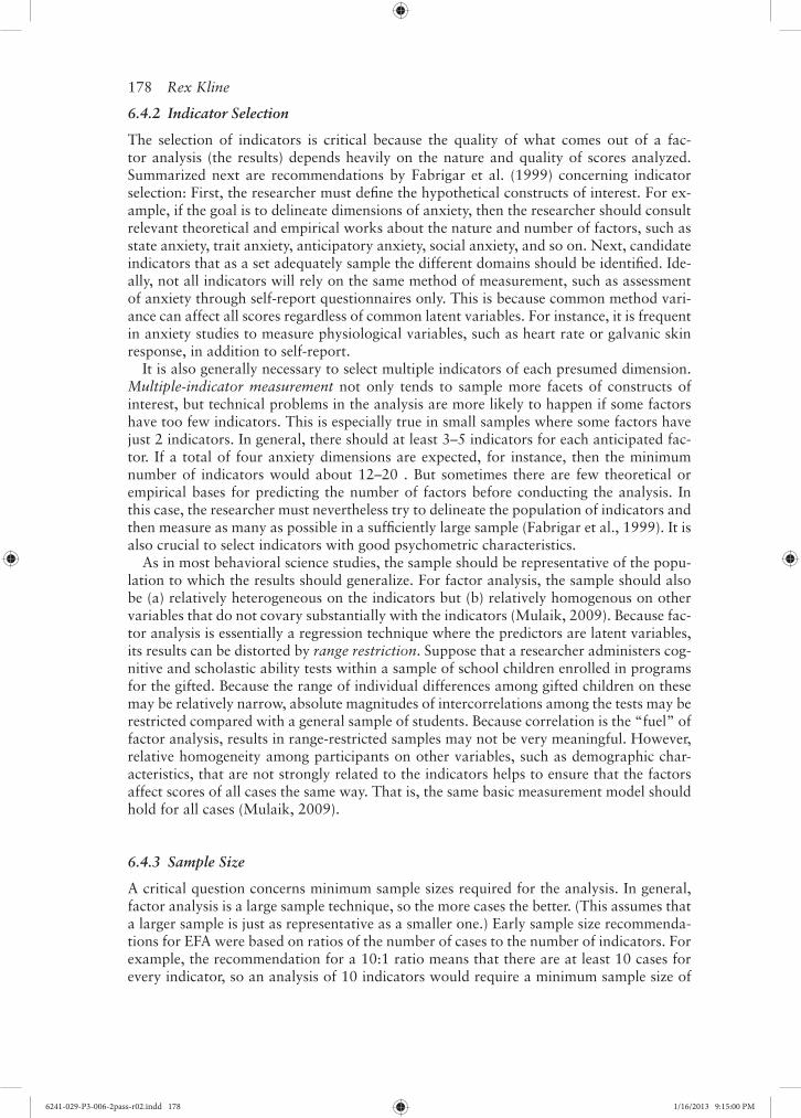
Figure 6.4 Scree plot for a principal components analysis of Kaufman Assessment Battery for Children–1st Edition subtests.
of 100% of the variance. A scree plot of the eigenvalues from the initial factors solution is presented in Figure 6.4.
The shape of the plot more or less levels out after extraction of the second factor, which is consistent with the specifi cation of a two-factor model. Values of all absolute residual correlations are < .05, which says that the two-factor model explains the observed cor-relations reasonably well. Because no raw data fi le was available for this analysis, the method of parallel analysis based on randomizing the scores cannot be applied. Reported
6241-029-P3-006-2pass-r02.indd 1886241-029-P3-006-2pass-r02.indd 188 1/16/2013 9:15:01 PM1/16/2013 9:15:01 PM
Exploratory and Confi rmatory Factor Analysis 189
in the right side of Table 6.2 are the eigenvalues and percentages of explained variance for the two factors extracted with PAF of the reduced correlation matrix. As expected, the eigenvalues for the two retained factors in the PAF solution are each lower the cor-responding fi rst two factors in the PCA solution. This happens because common vari-ance only is analyzed in PAF, but common variance is just a fraction of total variance (see Figure 6.1). Together the fi rst two PAF-extracted factors explain 48.97% of the total variance.
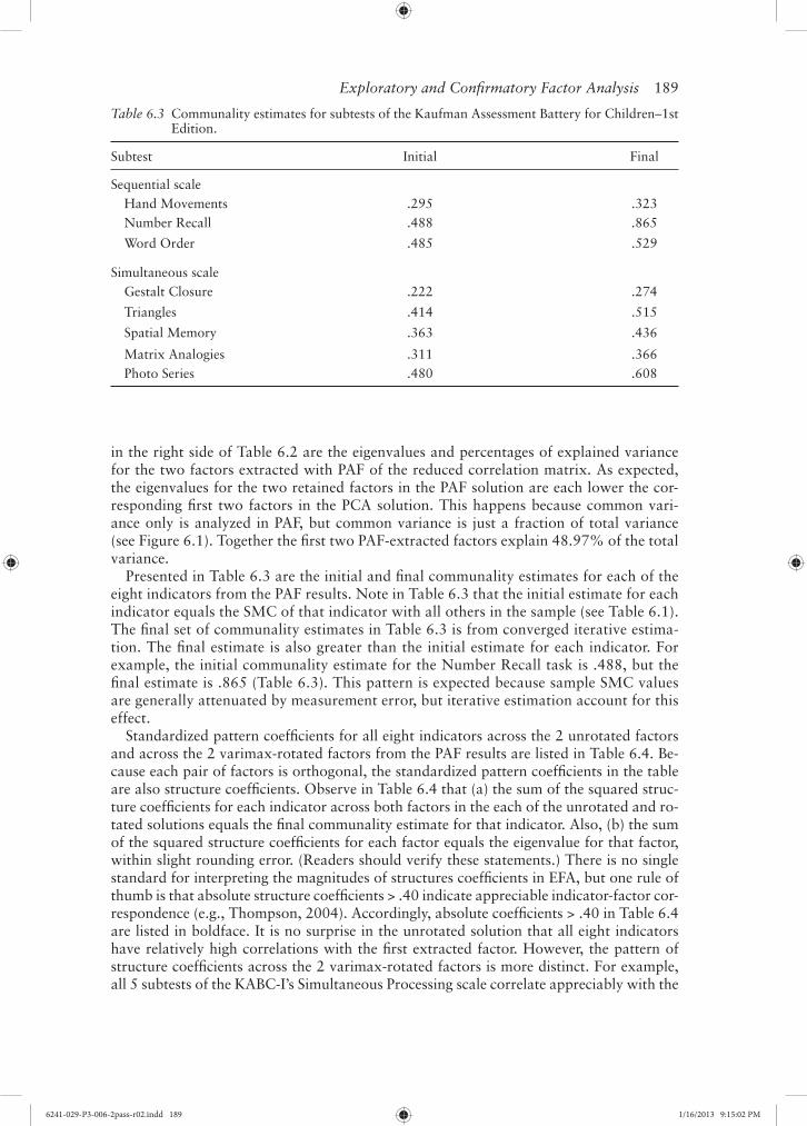
Presented in Table 6.3 are the initial and fi nal communality estimates for each of the eight indicators from the PAF results. Note in Table 6.3 that the initial estimate for each indicator equals the SMC of that indicator with all others in the sample (see Table 6.1). The fi nal set of communality estimates in Table 6.3 is from converged iterative estima-tion. The fi nal estimate is also greater than the initial estimate for each indicator. For example, the initial communality estimate for the Number Recall task is .488, but the fi nal estimate is .865 (Table 6.3). This pattern is expected because sample SMC values are generally attenuated by measurement error, but iterative estimation account for this effect.
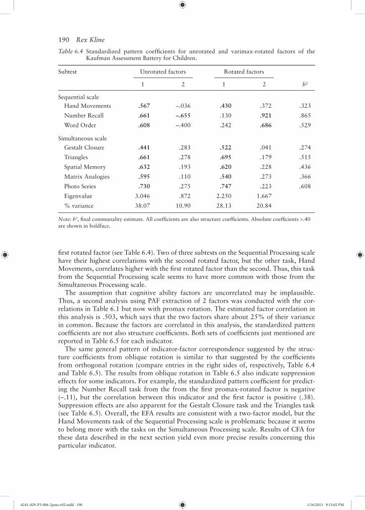
Standardized pattern coeffi cients for all eight indicators across the 2 unrotated factors and across the 2 varimax-rotated factors from the PAF results are listed in Table 6.4. Be-cause each pair of factors is orthogonal, the standardized pattern coeffi cients in the table are also structure coeffi cients. Observe in Table 6.4 that (a) the sum of the squared struc-ture coeffi cients for each indicator across both factors in the each of the unrotated and ro-tated solutions equals the fi nal communality estimate for that indicator. Also, (b) the sum of the squared structure coeffi cients for each factor equals the eigenvalue for that factor, within slight rounding error. (Readers should verify these statements.) There is no single standard for interpreting the magnitudes of structures coeffi cients in EFA, but one rule of thumb is that absolute structure coeffi cients > .40 indicate appreciable indicator-factor cor-respondence (e.g., Thompson, 2004). Accordingly, absolute coeffi cients > .40 in Table 6.4 are listed in boldface. It is no surprise in the unrotated solution that all eight indicators have relatively high correlations with the fi rst extracted factor. However, the pattern of structure coeffi cients across the 2 varimax-rotated factors is more distinct. For example, all 5 subtests of the KABC-I’s Simultaneous Processing scale correlate appreciably with the
Table 6.3 Communality estimates for subtests of the Kaufman Assessment Battery for Children–1st Edition.
Subtest Initial Final
Sequential scaleHand Movements .295 .323Number Recall .488 .865
Word Order .485 .529
Simultaneous scaleGestalt Closure .222 .274
Triangles .414 .515
Spatial Memory .363 .436
Matrix Analogies .311 .366Photo Series .480 .608
6241-029-P3-006-2pass-r02.indd 1896241-029-P3-006-2pass-r02.indd 189 1/16/2013 9:15:02 PM1/16/2013 9:15:02 PM
190 Rex Kline
fi rst rotated factor (see Table 6.4). Two of three subtests on the Sequential Processing scale have their highest correlations with the second rotated factor, but the other task, Hand Movements, correlates higher with the fi rst rotated factor than the second. Thus, this task from the Sequential Processing scale seems to have more common with those from the Simultaneous Processing scale.
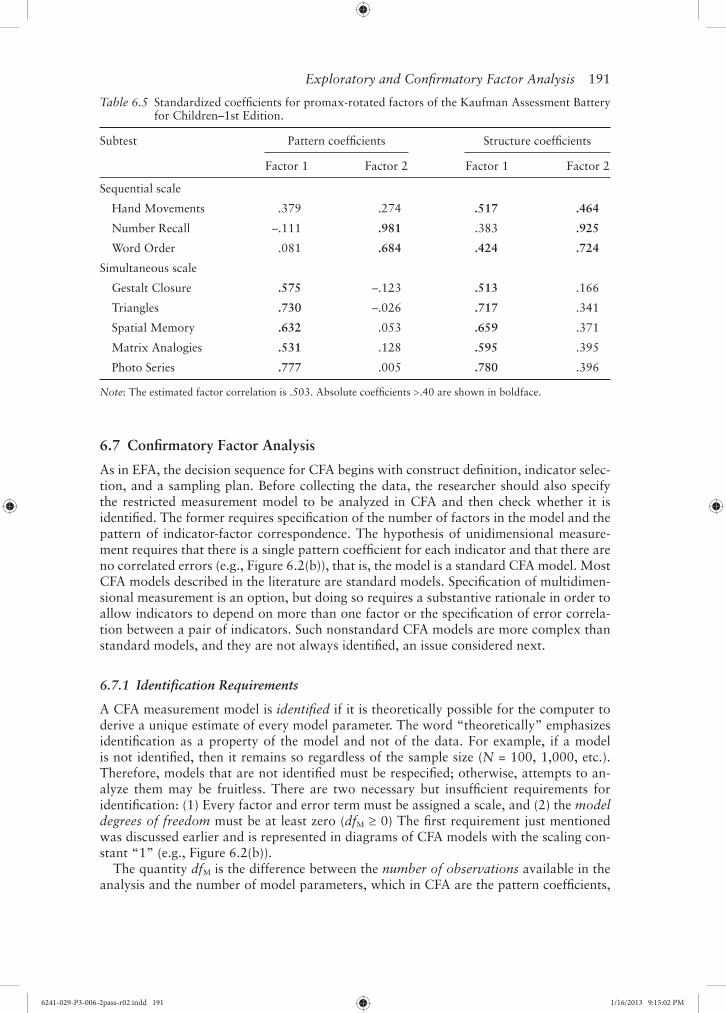
The assumption that cognitive ability factors are uncorrelated may be implausible. Thus, a second analysis using PAF extraction of 2 factors was conducted with the cor-relations in Table 6.1 but now with promax rotation. The estimated factor correlation in this analysis is .503, which says that the two factors share about 25% of their variance in common. Because the factors are correlated in this analysis, the standardized pattern coeffi cients are not also structure coeffi cients. Both sets of coeffi cients just mentioned are reported in Table 6.5 for each indicator.
The same general pattern of indicator-factor correspondence suggested by the struc-ture coeffi cients from oblique rotation is similar to that suggested by the coeffi cients from orthogonal rotation (compare entries in the right sides of, respectively, Table 6.4 and Table 6.5). The results from oblique rotation in Table 6.5 also indicate suppression effects for some indicators. For example, the standardized pattern coeffi cient for predict-ing the Number Recall task from the from the fi rst promax-rotated factor is negative (–.11), but the correlation between this indicator and the fi rst factor is positive (.38). Suppression effects are also apparent for the Gestalt Closure task and the Triangles task (see Table 6.5). Overall, the EFA results are consistent with a two-factor model, but the Hand Movements task of the Sequential Processing scale is problematic because it seems to belong more with the tasks on the Simultaneous Processing scale. Results of CFA for these data described in the next section yield even more precise results concerning this particular indicator.
Table 6.4 Standardized pattern coeffi cients for unrotated and varimax-rotated factors of the Kaufman Assessment Battery for Children.
Subtest Unrotated factors Rotated factors
1 2 1 2 h2
Sequential scaleHand Movements .567 –.036 .430 .372 .323
Number Recall .661 –.655 .130 .921 .865
Word Order .608 –.400 .242 .686 .529
Simultaneous scale
Gestalt Closure .441 .283 .522 .041 .274
Triangles .661 .278 .695 .179 .515
Spatial Memory .632 .193 .620 .228 .436
Matrix Analogies .595 .110 .540 .273 .366
Photo Series .730 .275 .747 .223 .608
Eigenvalue 3.046 .872 2.250 1.667
% variance 38.07 10.90 28.13 20.84
Note: h2, fi nal communality estimate. All coeffi cients are also structure coeffi cients. Absolute coeffi cients .40 are shown in boldface.
6241-029-P3-006-2pass-r02.indd 1906241-029-P3-006-2pass-r02.indd 190 1/16/2013 9:15:02 PM1/16/2013 9:15:02 PM
Exploratory and Confi rmatory Factor Analysis 191
6.7 Confi rmatory Factor Analysis
As in EFA, the decision sequence for CFA begins with construct defi nition, indicator selec-tion, and a sampling plan. Before collecting the data, the researcher should also specify the restricted measurement model to be analyzed in CFA and then check whether it is identifi ed. The former requires specifi cation of the number of factors in the model and the pattern of indicator-factor correspondence. The hypothesis of unidimensional measure-ment requires that there is a single pattern coeffi cient for each indicator and that there are no correlated errors (e.g., Figure 6.2(b)), that is, the model is a standard CFA model. Most CFA models described in the literature are standard models. Specifi cation of multidimen-sional measurement is an option, but doing so requires a substantive rationale in order to allow indicators to depend on more than one factor or the specifi cation of error correla-tion between a pair of indicators. Such nonstandard CFA models are more complex than standard models, and they are not always identifi ed, an issue considered next.
6.7.1 Identifi cation Requirements
A CFA measurement model is identifi ed if it is theoretically possible for the computer to derive a unique estimate of every model parameter. The word “theoretically” emphasizes identifi cation as a property of the model and not of the data. For example, if a model is not identifi ed, then it remains so regardless of the sample size (N = 100, 1,000, etc.). Therefore, models that are not identifi ed must be respecifi ed; otherwise, attempts to an-alyze them may be fruitless. There are two necessary but insuffi cient requirements for identifi cation: (1) Every factor and error term must be assigned a scale, and (2) the model degrees of freedom must be at least zero (dfM 0) The fi rst requirement just mentioned was discussed earlier and is represented in diagrams of CFA models with the scaling con-stant “1” (e.g., Figure 6.2(b)).
The quantity dfM is the difference between the number of observations available in the analysis and the number of model parameters, which in CFA are the pattern coeffi cients,
Table 6.5 Standardized coeffi cients for promax-rotated factors of the Kaufman Assessment Battery for Children–1st Edition.
Subtest Pattern coeffi cients Structure coeffi cients
Factor 1 Factor 2 Factor 1 Factor 2
Sequential scale
Hand Movements .379 .274 .517 .464
Number Recall –.111 .981 .383 .925
Word Order .081 .684 .424 .724
Simultaneous scale
Gestalt Closure .575 –.123 .513 .166
Triangles .730 –.026 .717 .341
Spatial Memory .632 .053 .659 .371
Matrix Analogies .531 .128 .595 .395
Photo Series .777 .005 .780 .396
Note: The estimated factor correlation is .503. Absolute coeffi cients .40 are shown in boldface.
6241-029-P3-006-2pass-r02.indd 1916241-029-P3-006-2pass-r02.indd 191 1/16/2013 9:15:02 PM1/16/2013 9:15:02 PM
192 Rex Kline
factor variances and covariances, and error variances and covariances. The number of observations is not the sample size. Instead, it is literally the number of entries in the data matrix in lower diagonal form where only the unique values of correlations or covari-ances are reported in the lower-left-hand side of the matrix. The number of observations is calculated as ni(ni + 1)/2, where ni is the number of indicators, not the sample size. For example, if there are ni = 4 indicators in a CFA model, then the number of observations is 4(5)/2, or 10. This count (10) equals the total number of diagonal and unique off-diagonal entries in the data matrix for 4 variables. With ni = 4, the greatest number of parameters that could be estimated by the computer is 10. Fewer parameters can be estimated in a more parsimonious model, but not > 10. Also, the number of observations has nothing to do with sample size. If four indicators are measured for 100 or 1,000 cases, the number of observations is still 10. Adding cases does not increase the number of observations; only adding indicators can do so.
In practice, researchers should analyze models with positive degrees of freedom (dfM 0). This is because identifi ed models with no degrees of freedom will perfectly fi t the data, that is, all residual correlations will equal zero. When dfM = 0, the model is just as complex as the data to be explained. Such models are uninteresting because they test no specifi c hypotheses. Models where dfM 0 generally do not have perfect fi t. This is because dfM 0 allows for the possibility of model-data discrepancies. Thus, retained models with greater degrees of freedom have withstood a greater potential for rejection. The idea underlies the parsimony principle: given two models with similar fi t to the same data, the simpler model is preferred, assuming that it is theoretically plausible. Thus, the goal is thus to fi nd a parsimonious measurement model with acceptably close fi t to the data.
Additional identifi cation requirements for standard CFA models concern the minimum number of indicators for each factor. A single-factor standard model requires at least three indicators in order to be identifi ed. However, one-factor models with just three indicators have no degrees of freedom, so their fi t to the data will be perfect, so in prac-tice, a one-factor model should have 4 indicators. A standard model with 2 factors requires at least two indicators per factor in order to be identifi ed. However, the analysis of CFA models where some factors have just two indicators is potentially problematic, so at least three indicators per factor is recommended.
The case concerning identifi cation for nonstandard CFA models is more compli-cated. This is because unlike standard models, nonstandard CFA models that satisfy all the requirements just described are not always identifi ed. In particular, specifying that an indicator depends on more than a single factor or that a pair of error terms is correlated is possible only if certain additional requirements are met. These extra requirements are summarized in the form of identifi cation heuristics for determining whether a nonstandard model is identifi ed (e.g., Kenny, Kashy, & Bolger, 1998; Kline, 2010, Chapter 6), but these heuristics are not always straightforward to apply for com-plex models with multiple correlated errors or indicators with 2 pattern coeffi cients. For example, in order for a model with error correlations to be identifi ed, each factor must have at minimum number of indicators whose errors are uncorrelated, but this minimum number is either two or three depending on patterns of error correlations and pattern coeffi cients among the other indicators. There are similar requirements for each pair of factors and for each indicator in a nonstandard model. The specifi cation of a single error correlation or that an indicator measures two factors in a CFA model that is otherwise standard may not cause a problem. This is another reason to specify an initial CFA model that is parsimonious: Simpler models are less likely to run into problems concerning identifi cation.
6241-029-P3-006-2pass-r02.indd 1926241-029-P3-006-2pass-r02.indd 192 1/16/2013 9:15:02 PM1/16/2013 9:15:02 PM
Exploratory and Confi rmatory Factor Analysis 193
6.7.2 Parameter Estimation
The default method in CFA is ML, which in SEM analyzes covariance matrices only and simultaneously estimates all model parameters in an iterative algorithm. Computer pro-cedures for ML estimation often begin iterative estimation by generating default initial estimates of certain model parameters known as start values. For example, the EQS pro-gram for SEM (including CFA) (Bentler, 2006) assumes in the fi rst iteration that all un-standardized pattern coeffi cients in CFA models equal 1.0. However, if default start values are grossly inaccurate, then iterative estimation may fail to converge. Fortunately, most SEM computer tools allow the user to specify start values other than the program’s default values. Better initial estimates may lead to a converged solution; see Kline (2010, p. 263) for guidelines on how to specify start values in CFA. If estimation converges successfully, it is still necessary to carefully look through the estimates for Heywood cases, just as in EFA when using PAF extraction.
The method of ML estimation assumes multivariate normality, and the method is not robust against violations of this assumption. This means that it is necessary to carefully screen the raw data and deal with problems, such as extreme outlier scores or severely nonnormal univariate distributions that contribute to multivariate nonnormality. Kline (2010, chapter 3) describes how to screen the data and prepare a “proper” matrix sum-mary for ML estimation. Many SEM computer tools can optionally use a corrected nor-mal theory method, which uses ML estimation to generate parameter estimates that are then corrected for the degree of skew or kurtosis in the data. These corrected methods require input of a raw data fi le, not a matrix summary. There are other, more specialized estimation methods for severely non-normal data or for indicators that are not continuous variables, such as when items are specifi ed as indicators in CFA models instead of scales. Some options for analyzing items-as-indicators in CFA are described in the next section.
6.7.3 Evaluation of Model Fit
There are two main classes of statistics in SEM that evaluate the correspondence between model and data, model test statistics and approximate fi t indexes. The former are sta-tistical tests of whether the covariance matrix implied by the researcher’s model is close enough to sample covariance matrix that the differences might reasonably be considered as due to sampling error. Most model test statistics are scaled such that higher values in-dicate increasingly poor model-data correspondence. Thus, it is a statistically signifi cant result (e.g., p < .05) that indicates problematic model–data correspondence. This logic is “backward” compared with most statistical tests where rejection of the null hypothesis supports the research hypothesis. But in SEM (and CFA, too) it is the lack of statistical signifi cance (e.g., p .05) that supports the researcher’s model. The most widely reported test statistic is the model chi-square, 2
M, with degrees of freedom that equal dfM, the
model degrees of freedom. The statistic 2M assumes multivariate normality, which is also
required in ML estimation.
In small samples, it can happen that the power of the model chi-square test is so low that it is diffi cult to correctly reject a false model (e.g., MacCallum et al., 1996). In very large samples, it can happen that
2M is statistically signifi cant even though the magnitudes of
model-data discrepancies are slight. For this reason, researchers in the past tended to ignore the results of the model chi-square test even in samples that were not very large. However, this practice is now viewed by more and more methodologists as excessively lax (e.g., Bar-rett, 2007). A better alternative is to consider a statistically signifi cant result as providing preliminary evidence against the model that must be further diagnosed. Likewise, a model
6241-029-P3-006-2pass-r02.indd 1936241-029-P3-006-2pass-r02.indd 193 1/16/2013 9:15:02 PM1/16/2013 9:15:02 PM
194 Rex Kline
chi-square test result that is not statistically signifi cant does not automatically lead to the decision to retain the model, especially if the sample size is not very large. Further evalua-tion of a model’s fi t to the data is also needed in this case (Kline, 2010).
The outcome of an approximate fi t index is not the dichotomous decision to reject or retain a null hypothesis. Instead, these indexes are intended as continuous measures of model-data correspondence. Some approximate fi t indexes are scaled such that lower values indicate closer model-data correspondence, but most are scaled so that it is higher values that suggest better fi t. And the metrics of some approximate fi t indexes are more-or-less standardized so that their range is 0–1.0 where a value of 1.0 indicates the best fi t. Philosophically, approximate fi t indexes are consistent with the view that truly correct models may not exist. That is, basically all statistical models are probably wrong to some degree because they are imperfect refl ections of a complex reality. Instead, models are ap-proximation tools that help researchers to structure their thinking about a phenomenon of interest. In contrast, a model test statistic is more analogous to a smoke detector: When the alarm sounds, there may or may not be a fi re (serious model-data discrepancy), but it is prudent to treat the alarm seriously (conduct more detailed diagnostic evaluation of fi t).
There are dozens of different approximate fi t indexes, but most break down into a few basic categories. Briefl y, absolute fi t indexes are generally interpreted as proportions of the covariances in the sample data matrix explained by the model. However, explanatory power at the level of data matrix has little to do with whether the model accounts for relatively high proportions of the variance in the indicators. Incremental fi t indexes indi-cate the relative improvement in fi t of the researcher’s model compared with a statistical baseline model where it is assumed that all observed variables are uncorrelated. But the as-sumption of zero covariances among indicators of a measurement model is implausible in most cases. Parsimony-adjusted fi t indexes includes in their equations a built-in “penalty” for complexity related to the value of dfM. (Recall that more parsimonious models have higher degrees of freedom.) And predictive fi t indexes estimate model fi t in hypothetical replication samples randomly drawn from the same population, but most applications of CFA do not call for this type of fi t index.
Based on the results of some computer simulation studies conducted in the 1980s and 1990s about the behavior of approximate fi t indexes under varying data and model con-ditions, many researchers relied on a series of rules of thumb or threshold values of ap-proximate fi t indexes that supposedly indicated “good” fi t of the model to the data. An example of a threshold for the hypothetical XYZ index scaled from 0–1.0 would be, if XYZ > .90, then conclude “good” fi t. At the same time that researchers increasingly relied on threshold values for approximate fi t indexes, they also tended to ignore model test statistics. Unfortunately, results of more recent simulation studies indicate that (1) the ac-curacy of thresholds depend on the particular type of structural equation model studied, (2) expected values of approximate fi t indexes have little relation to their threshold values when distributional assumptions are violated, and (3) there is little direct relation between values of fi t statistics of any type (including model test statistics) and the degree or type of misspecifi cation (e.g., Millsap, 2007). The point just mentioned explains why researchers should also provide more specifi c information about model fi t. Perhaps the best way to do is to report the matrix of residual correlations, which say something about model fi t at a more fundamental level than summary fi t statistics (Kline, 2010). As in EFA, absolute residual correlations > .10 in CFA suggest poor explanation of the observed correlation between that pair of indicators.
Briefl y described next are approximate fi t indexes the values of which should be reported in most analyses; see Kline (2010, chap. 8) for more information. Threshold values are given for each index, but readers should not reify these values in view of the issues just raised.
6241-029-P3-006-2pass-r02.indd 1946241-029-P3-006-2pass-r02.indd 194 1/16/2013 9:15:02 PM1/16/2013 9:15:02 PM
Exploratory and Confi rmatory Factor Analysis 195
The Steiger-Lind root mean square error of approximation (RMSEA) is a parsimony-corrected index that in computer output is usually reported with a 90% confi dence in-terval, which takes account of sample size. Unlike 2
M, the RMSEA theoretically follows a noncentral chi-square distribution that allows for a certain degree of discrepancy between population and sample models. The best result is RMSEA = 0, and higher values indicate in-creasingly worse fi t of the model to the data. If the value of the upper bound of the confi dence interval based on the RMSEA exceeds .10, then problematic model-data correspondence may be indicated. The Bentler comparative fi t index (CFI) is an incremental fi t index that measures the relative improvement in fi t of the researcher’s model over that of a baseline model that assumes uncorrelated indicators. Like the RMSEA, the CFI allows for some dis-crepancy between population and sample models. Values of the CFI range from 0–1.0 where 1.0 is the best result. The standardized root mean square residual (SRMR) is a measure of the mean absolute residual correlation, so values close to 0 are a better result. Ideally, the value of the CFI should exceed .95 or so, and the value of the SRMR should be < .10.
6.7.4 Model Respecifi cation
If the fi t of an initial CFA model to the data is poor, then the analysis enters the respecifi ca-tion phase where alternative models are generated and then fi tted to the same data matrix. There are two general types of respecifi cation options. The fi rst concerns the correspon-dence between indicators and factors. The basic possibilities here include the respecifi ca-tions that an indicator (a) loads on an additional factor, (b) depends on a different factor, or (c) shares has an error correlation with another indicator, all compared with the origi-nal model. The second category for respecifi cation concerns the factors. For example, the researcher may have specifi ed the wrong number of factors. Poor discriminant validity as evidenced by very high factor correlations may indicate that the model has too many factors. On the other hand, poor convergent validity within sets of indicators of the same factor suggests that the model may have too few factors.
Respecifi cation should be guided by the same theoretical and empirical bases that sup-ported the specifi cation of the original model. At the same time researchers often inspect certain types of output that may inform respecifi cation. Inspecting the pattern of residual correlations may shed light on the question of indicator-factor correspondence. Suppose that indicator X4 is specifi ed to measure factor A but (a) the residual correlations between it and all the indicators of factor B are large and positive and (b) the pattern coeffi cient for the A X4 is reasonably large. This pattern suggests that X4 may measure both factors. A different possibility when there is a large residual correlation for a pair of indicators is that their specifi c variances overlap, or their error terms covary.
Most SEM computer tools can optionally print values of modifi cation indexes, which are interpreted as chi-square statistics with a single degree of freedom, or 2 (1). A modifi cation index estimates the amount by which the overall model chi-square would decrease if a previously-fi xed-to-zero parameter were freely estimated, which adds the corresponding effect to the model. Suppose for a two-factor model that X4 is specifi ed to measure factor A but not factor B. In this model, the parameter B X4 is specifi ed to equal 0. If the modifi cation index for this parameter equals 5.50, then (a) it is estimated that the value of
2M will decrease by 5.5 points if the param-
eter B X4 were added to the model and (b) the amount of this decrease would be statistically signifi cant because 2 (1) = 5.50, p .05. However, the researcher must avoid respecifying the model based solely on modifi cation indexes. This is because these statistics capitalize heavily on sample-specifi c variation, and respecifi cation that
6241-029-P3-006-2pass-r02.indd 1956241-029-P3-006-2pass-r02.indd 195 1/16/2013 9:15:02 PM1/16/2013 9:15:02 PM
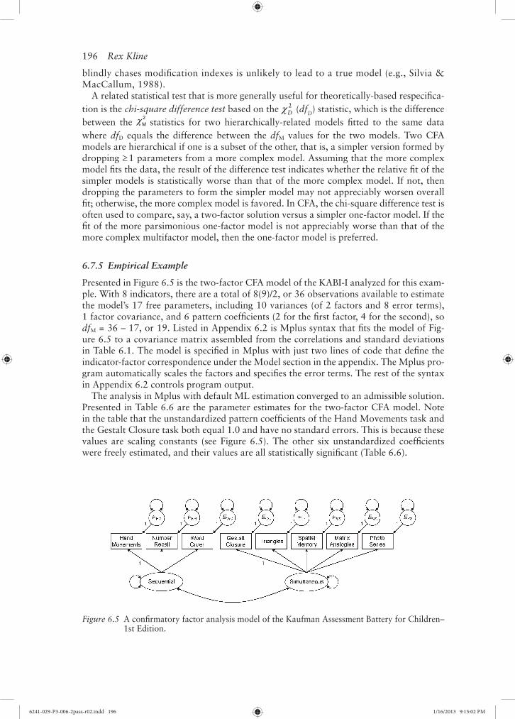
196 Rex Kline
blindly chases modifi cation indexes is unlikely to lead to a true model (e.g., Silvia & MacCallum, 1988).
A related statistical test that is more generally useful for theoretically-based respecifi ca-tion is the chi-square difference test based on the 2
D (dfD) statistic, which is the difference between the 2
M statistics for two hierarchically-related models fi tted to the same data where dfD equals the difference between the dfM values for the two models. Two CFA models are hierarchical if one is a subset of the other, that is, a simpler version formed by dropping 1 parameters from a more complex model. Assuming that the more complex model fi ts the data, the result of the difference test indicates whether the relative fi t of the simpler models is statistically worse than that of the more complex model. If not, then dropping the parameters to form the simpler model may not appreciably worsen overall fi t; otherwise, the more complex model is favored. In CFA, the chi-square difference test is often used to compare, say, a two-factor solution versus a simpler one-factor model. If the fi t of the more parsimonious one-factor model is not appreciably worse than that of the more complex multifactor model, then the one-factor model is preferred.
6.7.5 Empirical Example
Presented in Figure 6.5 is the two-factor CFA model of the KABI-I analyzed for this exam-ple. With 8 indicators, there are a total of 8(9)/2, or 36 observations available to estimate the model’s 17 free parameters, including 10 variances (of 2 factors and 8 error terms), 1 factor covariance, and 6 pattern coeffi cients (2 for the fi rst factor, 4 for the second), so dfM = 36 – 17, or 19. Listed in Appendix 6.2 is Mplus syntax that fi ts the model of Fig-ure 6.5 to a covariance matrix assembled from the correlations and standard deviations in Table 6.1. The model is specifi ed in Mplus with just two lines of code that defi ne the indicator-factor correspondence under the Model section in the appendix. The Mplus pro-gram automatically scales the factors and specifi es the error terms. The rest of the syntax in Appendix 6.2 controls program output.
The analysis in Mplus with default ML estimation converged to an admissible solution. Presented in Table 6.6 are the parameter estimates for the two-factor CFA model. Note in the table that the unstandardized pattern coeffi cients of the Hand Movements task and the Gestalt Closure task both equal 1.0 and have no standard errors. This is because these values are scaling constants (see Figure 6.5). The other six unstandardized coeffi cients were freely estimated, and their values are all statistically signifi cant (Table 6.6).
Figure 6.5 A confi rmatory factor analysis model of the Kaufman Assessment Battery for Children–1st Edition.
6241-029-P3-006-2pass-r02.indd 1966241-029-P3-006-2pass-r02.indd 196 1/16/2013 9:15:02 PM1/16/2013 9:15:02 PM

Exploratory and Confi rmatory Factor Analysis 197
Standardized pattern coeffi cients are also reported in the table.5 Because each indica-tor depends on a single factor, these standardized pattern coeffi cients are also structure coeffi cients. The estimated factor correlation is .557 (see Table 6.6) which is similar to the corresponding result in EFA with an oblique rotation, .503.
Reported in Table 6.7 are values of structure coeffi cients for all 8 indicators of the KABC-I. Coeffi cients presented in boldface in the table are also standardized pattern co-effi cients for indicators specifi ed to measure either factor. For example, the Hand Move-ments task is not specifi ed to measure simultaneous processing; therefore, the pattern coeffi cient for the Hand Movements-simultaneous factor correspondence is zero (see Figure 6.5). However, the structure coeffi cients for the Hand Movements task are .497 and
Table 6.6 Maximum likelihood estimates for a confi rmatory two-factor model of the Kaufman Assessment Battery for Children–1st Edition.
Parameter Unstandardized SE Standardized
Pattern coeffi cientsSequential factor
Hand Movements 1.000 a — .497
Number Recall 1.147 .181 .807
Word Order 1.388 .219 .808
Simultaneous factor
Gestalt Closure 1.000 a — .503
Triangles 1.445 .227 .726
Spatial Memory 2.029 .335 .656
Matrix Analogies 1.212 .212 .588
Photo Series 1.727 .265 .782
Measurement error variances
Hand Movements 8.664 .938 .753
Number Recall 1.998 .414 .349
Word Order 2.902 .604 .347
Gestalt Closure 5.419 .585 .747
Triangles 3.425 .458 .472
Spatial Memory 9.998 1.202 .570
Matrix Analogies 5.104 .578 .654
Photo Series 3.483 .537 .389
Factor variances and covariance
Sequential 2.839 .838 1.000
Simultaneous 1.835 .530 1.000
Sequential Simultaneous 1.271 .324 .557
Note: Standardized estimates for measurement errors are proportions of unexplained variance.a Not tested for statistical signifi cance. All other unstandardized estimates are statistically signifi cant at p .01.
6241-029-P3-006-2pass-r02.indd 1976241-029-P3-006-2pass-r02.indd 197 1/16/2013 9:15:03 PM1/16/2013 9:15:03 PM
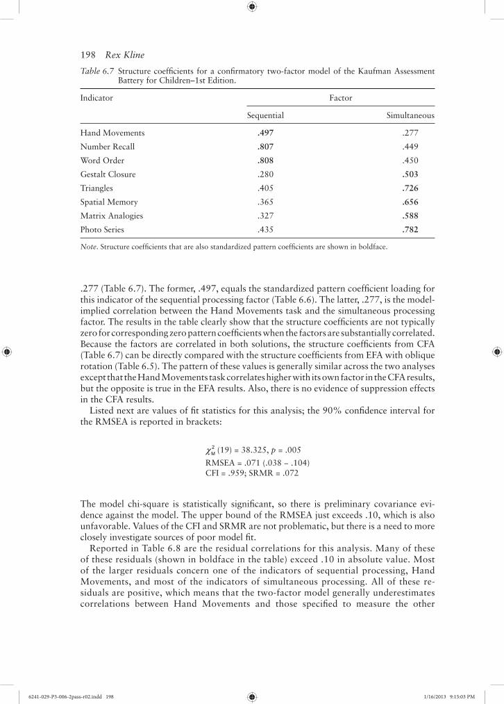
198 Rex Kline
.277 (Table 6.7). The former, .497, equals the standardized pattern coeffi cient loading for this indicator of the sequential processing factor (Table 6.6). The latter, .277, is the model-implied correlation between the Hand Movements task and the simultaneous processing factor. The results in the table clearly show that the structure coeffi cients are not typically zero for corresponding zero pattern coeffi cients when the factors are substantially correlated. Because the factors are correlated in both solutions, the structure coeffi cients from CFA (Table 6.7) can be directly compared with the structure coeffi cients from EFA with oblique rotation (Table 6.5). The pattern of these values is generally similar across the two analyses except that the Hand Movements task correlates higher with its own factor in the CFA results, but the opposite is true in the EFA results. Also, there is no evidence of suppression effects in the CFA results.
Listed next are values of fi t statistics for this analysis; the 90% confi dence interval for the RMSEA is reported in brackets:
Table 6.7 Structure coeffi cients for a confi rmatory two-factor model of the Kaufman Assessment Battery for Children–1st Edition.
Indicator Factor
Sequential Simultaneous
Hand Movements .497 .277
Number Recall .807 .449
Word Order .808 .450
Gestalt Closure .280 .503
Triangles .405 .726
Spatial Memory .365 .656
Matrix Analogies .327 .588
Photo Series .435 .782
Note. Structure coeffi cients that are also standardized pattern coeffi cients are shown in boldface.
2M (19) = 38.325, p = .005
RMSEA = .071 (.038 − .104)CFI = .959; SRMR = .072
The model chi-square is statistically signifi cant, so there is preliminary covariance evi-dence against the model. The upper bound of the RMSEA just exceeds .10, which is also unfavorable. Values of the CFI and SRMR are not problematic, but there is a need to more closely investigate sources of poor model fi t.
Reported in Table 6.8 are the residual correlations for this analysis. Many of these of these residuals (shown in boldface in the table) exceed .10 in absolute value. Most of the larger residuals concern one of the indicators of sequential processing, Hand Movements, and most of the indicators of simultaneous processing. All of these re-siduals are positive, which means that the two-factor model generally underestimates correlations between Hand Movements and those specifi ed to measure the other
6241-029-P3-006-2pass-r02.indd 1986241-029-P3-006-2pass-r02.indd 198 1/16/2013 9:15:03 PM1/16/2013 9:15:03 PM
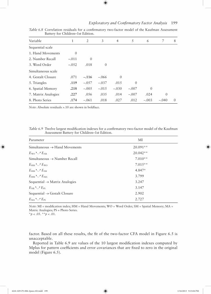
Exploratory and Confi rmatory Factor Analysis 199
Table 6.8 Correlation residuals for a confi rmatory two-factor model of the Kaufman Assessment Battery for Children–1st Edition.
Variable 1 2 3 4 5 6 7 8
Sequential scale
1. Hand Movements 0
2. Number Recall –.011 0
3. Word Order –.052 .018 0
Simultaneous scale
4. Gestalt Closure .071 –.116 –.066 0
5. Triangles .119 –.057 –.037 .015 0
6. Spatial Memory .218 –.005 –.015 –.030 –.007 0
7. Matrix Analogies .227 .056 .035 .014 –.007 .024 0
8. Photo Series .174 –.061 .018 .027 .012 –.003 –.040 0
Note: Absolute residuals >.10 are shown in boldface.
Table 6.9 Twelve largest modifi cation indexes for a confi rmatory two-factor model of the Kaufman Assessment Battery for Children–1st Edition.
Parameter MI
Simultaneous Hand Movements 20.091**
EWO ENR 20.042**
Simultaneous Number Recall 7.010**
EHM EWO 7.015**
EHM ESM 4.847*
EHM EMA 3.799
Sequential Matrix Analogies 3.247
ENR EPS 3.147
Sequential Gestalt Closure 2.902
EMA EPS 2.727
Note: MI = modifi cation index; HM = Hand Movements; WO = Word Order; SM = Spatial Memory; MA = Matric Analogies; PS = Photo Series. *p < .05. **p < .01.
factor. Based on all these results, the fi t of the two-factor CFA model in Figure 6.5 is unacceptable.
Reported in Table 6.9 are values of the 10 largest modifi cation indexes computed by Mplus for pattern coeffi cients and error covariances that are fi xed to zero in the original model (Figure 6.5).
6241-029-P3-006-2pass-r02.indd 1996241-029-P3-006-2pass-r02.indd 199 1/16/2013 9:15:04 PM1/16/2013 9:15:04 PM
200 Rex Kline
Note in the table that the 2 (1) statistics for the paths
Simultaneous Hand Movements and EWO ENR
are nearly identical (respectively, 20.091 and 20.042). Thus, either allowing the Hand Movements task to also depend on the simultaneous processing factor or adding an error covariance between the Word Order and Number Recall tasks would reduce the value of 2
M by about 20 points. Among other respecifi cations suggested by the modifi cation indexes, two have nearly the same 2(1) value: allow Number Recall to also load on the sequential processing factor (7.010), or allow the errors of the Hand Movements and Word Order tasks to covary (7.015) (Table 6.9). Obviously, the researcher needs some rationale for choosing among these potential respecifi cations. Based on my knowledge of the KABC-I and results of other studies (e.g., Keith, 1985), allowing the Hand Movements task to load on both factors is plausible.
For this example, the fi t of the EFA model was better than the fi t of the CFA model to the same data. This is not unexpected because the EFA model allows each indicator to load on both factors, but the CFA model specifi es unidimensional measurement. This is one reason why the specifi cation of a CFA model based on EFA outcomes and analyzed with the same data may lead to the rejection of the CFA model (van Prooijen & van der Kloot, 2001). That is, CFA does not generally “confi rm” the results of EFA. But the CFA results made more obvious the sources of poor fi t, which concern mainly the three indica-tors of the sequential processing factor.
6.8 Other Issues
Considered next are some additional issues and analysis options in factor analysis.
6.8.1 Items as Indicators
Likert-scale items are not generally continuous variables, and Pearson correlations may not be the best measure of association for them. This is especially true for items with binary response formats (e.g., true-false). Results of some computer simulation studies indicate that estimates from standard estimation methods for continuous variables may be inaccurate when the indicators are binary or ordinal variables. These simulation stud-ies generally assume a true population measurement model with continuous indicators. Within generated samples, the indicators are categorized to approximate data from non-continuous variables. Bernstein and Teng (1989) found that when there is only a single factor in the population but the indicators have few categories, one-factor measurement models tend to be rejected too often. That is, categorization can spuriously suggest the presence of multiple factors. DiStefano (2002) found that ML parameter estimates and their standard errors were both generally too low when the data analyzed are from cat-egorical indicators, and the degree of negative bias was higher as distributions became increasingly non-normal.
There are special estimation methods for analyzing ordinal indicators, such as items, available in some SEM computer tools, including EQS, LISREL, and Mplus (see Chapter 7 on Item Response Theory). These methods do not solely rely on ML estimation. Instead, they feature alternative estimators based on weighted least squares methods (e.g., Kline, 2010, chap. 7). These methods may be applied to a matrix of tetrachoric correlations or polychoric correlations, not Pearson correlations. A tetrachoric correlation is for two dichotomous variables, and it estimates what the Pearson r would be if both variables
6241-029-P3-006-2pass-r02.indd 2006241-029-P3-006-2pass-r02.indd 200 1/16/2013 9:15:04 PM1/16/2013 9:15:04 PM
Exploratory and Confi rmatory Factor Analysis 201
were continuous and normally distributed. A polychoric correlation is the generalization of the tetrachoric correlation that estimates r for ordinal variables with 2 levels. Some computer procedures, such as the PRELIS program of LISREL, can export polychoric or tetrachoric correlation matrices for analysis in a different program. Another option is to analyze parcels instead of items. A parcel is a total score across a set of homogenous items each with a Likert-type format. Parcels are generally treated as continuous variables, and analyzing a Pearson correlation matrix based on parcels is not problematic. The score reliability of parcels (total scores) tends to be greater than that for the individual items. However, it is critical that the items in each parcel are homogeneous, or unidimensional; otherwise, the results may be misleading. There are also different ways to parcel items, including random assignment of items to parcels and groupings of items based on rational grounds, and the choice can affect the results; see T. Little, Cunningham, Shahar, and Wi-daman (2002) for more information.
Another complication of item-level factor analysis is that easy or frequently endorsed items tend to form factors that are distinct from other factors made up of harder or less commonly endorsed items (Nunnally & Bernstein, 1994). Such factors may refl ect differ-ential response base rates more than they mirror substantive latent variables. In this case, a multifactor solution would be spurious, rendering subsequent interpretations incorrect. The researcher should inspect the response of items that form different factors. If these rates vary systematically over the factors, then the results may be due more to statistical than substantive bases (O’Connor, n.d.).
6.8.2 Factor Scores
When raw data are analyzed, it is possible to calculate factor scores for each case. Because factors are not directly measured but instead through their indicators, such scores are only estimates of cases’ relative standings on the factors. There is more than one way to calcu-late factor scores, however, and although scores derived using different methods tend to be highly correlated, they generally do not all yield identical rank orderings of the cases. For example, given structure coeffi cients, the technique of multiple regression can be used to derive estimated factor scores that are weighted combinations of the indicators and the factor. The weights derived in regression are those that lead to the closest correspondence between the factors and the estimated factor scores. Other methods for oblique solutions constrain the correlations among the factor scores to match those of the corresponding factors. Given that there is more than one way to derive estimated factor scores, Bollen’s (1989) perspective on this matter is relevant: Researchers should probably refrain from making too fi ne a comparison on estimated factor scores. See Grice (2001) for more infor-mation about factor scores.
Factor scores are calculated in EFA more often than in CFA. One reason is that scores derived in EFA tend to be used as either predictors or outcomes in subsequent analy-ses that involve other variables. In contrast, factors in structural equation models can be represented as either predictors or outcomes of other variables in the model, latent or observed. Such models are not CFA models—they are actually structural regression models—but it is no special problem in SEM to estimate regression coeffi cients for effects between latent variables without having to calculate factor scores.
6.8.3 Measurement Invariance
There are methods for both EFA and CFA for evaluating measurement invariance, which concerns whether scores from the operationalization of a construct have the same meaning
6241-029-P3-006-2pass-r02.indd 2016241-029-P3-006-2pass-r02.indd 201 1/16/2013 9:15:05 PM1/16/2013 9:15:05 PM

202 Rex Kline
under different conditions (Meade & Lautenschlager, 2004). These different conditions could involve consistency of measurement over populations, time of measurement, or methods of test administration (e.g., computer-administered vs. paper-and-paper format). Invariance over populations is related to the concept of construct bias, which implies that a test measures something different in one group (e.g., men) than in another (women). If not (i.e., there is no evidence for construct bias), then measurement is invariant over groups.
One method for testing invariance in EFA described by B. Thompson (2004, Chapter 8) involves best-fi t rotation where the factor solution in one sample is specifi ed as the target structure and the factor solution in a different sample is rotated to match the target struc-ture as close as possible. (This assumes the same number of factors is retained in both sam-ples.) The method derives a new matrix of pattern coeffi cients and structure coeffi cients for the non-target sample and also calculates factor correlations across the two samples. If the cross-sample factor correlations are low or there is no match of the pattern/structure coeffi cients across the groups, then measurement is not invariant.
The method of CFA offers even more precise tests of measurement invariance. One rea-son is that it is possible in CFA to estimate mean contrasts on latent variables across 2 groups in a cross-sectional design or across 2 measurement occasions in longitudinal design for a given factor model. When means are analyzed in CFA, the model has a mean structure that represents factor mean differences and indicator intercepts for regression of the indicators on the factors in addition to the model’s covariance structure. So specifi ed, a CFA model analyzed across multiple groups can be tested for various levels of measure-ment invariance. The most basic kind is confi gural invariance or equal form invariance. It is tested by specifying the same measurement model across the groups. In this model, both the number of factors and the factor-indicator correspondence are the same, but all parameters are freely estimated within each sample. If this model does not fi t the data, then measurement invariance does not hold at any level. A stronger of form of invariance is construct-level metric invariance, which means that the unstandardized pattern coef-fi cients of each indicator are equal within the bounds of sampling error across the groups. If the construct-level metric invariance hypothesis is retained, then the researcher could conclude that the constructs are manifested the same way in each group. If some, but not all, of the pattern coeffi cients are equal, then there is evidence for partial measurement invariance. It also possible in CFA to test for invariance concerning factor variances and covariances, error variances and covariances, and indicator intercepts; see Kline (2010, chapters 9, 11) for examples.
6.8.4 Multilevel Factor Analysis
There are versions of both EFA and CFA for analyzing measurement models in hierarchi-cal (nested) data sets where (a) scores are clustered into larger units and (b) scores within each level may not be independent. Suppose that data are collected from high school students who attend a total of 100 different schools. Students within each school are pre-sumably affected by common characteristics that include the curriculum, teaching staff, school policies about discipline, student-to-teacher ratios, physical resources of the school, and so on. Scores from students who attend the same school may not be independent, and one aim of multilevel modeling or hierarchical linear modeling is to adjust the statistical estimates for the degree of score dependencies. Multilevel techniques are also used to estimate contextual effects of higher-order variables on scores of individuals in a hierar-chical data set. An example in a multilevel factor analysis could be whether differences in student-teacher ratios between schools predicts the magnitude of covariation between
6241-029-P3-006-2pass-r02.indd 2026241-029-P3-006-2pass-r02.indd 202 1/16/2013 9:15:05 PM1/16/2013 9:15:05 PM
Exploratory and Confi rmatory Factor Analysis 203
indicators and factors within schools. Some SEM computer tools, including EQS, LISREL, and Mplus, support multilevel factor analysis, but the Mplus program is especially fl exible in analyzing either exploratory or confi rmatory measurement models in hierarchical data sets. See Heck and Thomas (2008) for an introduction to multilevel factor analysis.
6.9 Best Practices Summary
Some best practices for factor analysis are briefl y summarized: Report enough summary statistics, such as indicator correlations, standard deviations, and means, so that a reader could reproduce the results or test alternative models. Clearly spell out the rationale for indicator selection, measurement, model specifi cation, data characteristics including score reliabilities, and whether statistical assumptions are verifi ed. Avoid applying factor analy-sis in samples that are just too small. Give specifi c details about decision points in the analysis. For example, state the data matrix analyzed, the method of factor extraction (EFA) or estimation (CFA), and the criteria for retaining a certain number of factors and selecting a particular rotation method (EFA). Report both the unstandardized solution and the standardized solution (with the appropriate standard errors) when analyzing a covariance matrix. If an initial model is respecifi ed, inform readers about the theoretical or empirical justifi cations for these modifi cations. If no factor model is eventually retained, then explain what may be wrong with the theoretical foundations of the original model. Before using factor analysis, the researcher should thoroughly study the technique either in a course, professional workshop, or self study, but he or she should be open to a pro-cess of continual learning. Along these lines, B. Thompson (2004) gives concise and clear introductions to EFA and CFA, Brown (2006) describes CFA for applied researchers, and Mulaik (2009) provides a comprehensive treatment of EFA for readers with strong quan-titative backgrounds.
Notes
1. There are freely available (after registration) online reviews of correlation and regression funda-mentals available at http://www.statisticalassociates.com/
2. O’Connor (2000) describes SPSS and SAS/STAT macros for parallel analysis that can be freely downloaded from https://people.ok.ubc.ca/brioconn/nfactors/nfactors.html
3. Keith (1985) suggested alternative names for the factors in the KABC-I’s theoretical model, in-cluding short-term memory instead of sequential processing and visual-spatial reasoning instead of simultaneous processing. These different names for the same factors should remind all us to avoid the naming fallacy.
4. Readers can freely download all syntax, data, and output fi les in either plain text or Adobe PDF formats for both empirical examples (EFA, CFA) in this chapter from http://psychology.concordia.ca/fac/kline/efa&cfa.html
5. The Mplus program can optionally print standard errors for standardized estimates, but these values are not reported in Table 6.6.
References
Barrett, P. (2007). Structural equation modelling: Adjudging model fi t. Personality and Individual Differences, 42, 815–824. doi:10.1016/j.paid.2006.09.018
Bentler, P. M. (2006). EQS 6 structural equations program manual. Encino, CA: Multivariate Software.
Bernstein, I. H., & Teng, G. (1989). Factoring items and factoring scales are different: Spurious evi-dence for multidimensionality due to item categorization. Psychological Bulletin, 105, 467–477. doi:10.1037//0033-2909.105.3.467
6241-029-P3-006-2pass-r02.indd 2036241-029-P3-006-2pass-r02.indd 203 1/16/2013 9:15:05 PM1/16/2013 9:15:05 PM
204 Rex Kline
Bollen, K. A. (1989). Structural equations with latent variables. New York, NY: Wiley.Brown, T. A. (2006). Confi rmatory factor analysis for applied research. New York, NY: Guilford
Press.Costello, A. B., & Osborne, J. W. (2005). Best practices in exploratory factor analysis: Four recom-
mendations for getting the most from your analysis. Practical Assessment, Research & Evalua-tion, 10(7). Retrieved from http://pareonline.net/
Crawford, A. V., Green, S. B., Levy, R., Lo, W., Scott, L., Svetina, D., & Thompson, M. S. (2010). Evaluation of parallel analysis methods for determining the number of factors. Educational and Psychological Measurement, 70, 885–901. doi:10.1177/001316441037933
DiStefano, C. (2002). The impact of categorization with confi rmatory factor analysis. Structural Equation Modeling, 9, 327–346. doi:10.1207/S15328007sem0903_2
Fabrigar, L. R., Wegener, D. T., MacCallum, R. C., & Strahan, E. J. (1999). Evaluating the use of exploratory factor analysis in psychological research psychological methods. Psychological Meth-ods, 4, 272–299. doi:10.1037/1082-989X.4.3.272
Furfey, P. H., & Daly, J. F. (1937). A criticism of factor analysis as a technique of social research. American Sociological Review, 2, 178–186. doi:10.2307/2083471
Graham, J. M., Guthrie, A. C., & Thompson, B. (2003). Consequences of not interpreting structure coeffi cients in published CFA research: A reminder. Structural Equation Modeling, 10, 142–153. doi:10.1207/S15328007SEM1001_7
Grice, J. W. (2001). Computing and evaluating factor scores. Psychological Methods, 6, 430–450. doi: 10.1037/1082-989X.6.4.430
Heck, R. H., & Thomas, S. L. (2008). An introduction to multilevel modeling techniques (2nd ed.). New York, NY: Routledge.
IBM Corp. (2012). IBM SPSS Statistics for Windows (release 21.0) [Computer software]. Armonk, NY: Author.
Jackson, D. L. (2003). Revisiting sample size and number of parameter estimates: Some sup-port for the N:q hypothesis. Structural Equation Modeling, 10, 128–141. doi:10.1207/S15328007SEM1001_6
Jöreskog, K.G., & Sörbom, D. (2012). LISREL 9.1 for Windows [Computer software]. Skokie, IL: Scientifi c Software International.
Kaufman, A. S., & Kaufman, N. L. (1983). K-ABC administration and scoring manual. Circle Pines, MN: American Guidance Service.
Keith, T. Z. (1985). Questioning the K-ABC: What does it measure? School Psychology Review, 14, 9–20.
Kenny, D. A., Kashy, D. A., & Bolger, N. (1998). Data analysis in social psychology. In D. Gilbert, S. Fiske, & G. Lindzey (Eds.), The handbook of social psychology (Vol. 1, 4th ed., pp. 233–265). Boston, MA: McGraw-Hill.
Kline, R. B. (2010). Principles and practice of structural equation modeling (3rd ed.). New York, NY: Guilford Press.
Little, T. D., Cunningham, W. A., Shahar, G., & Widamin, K. F. (2002). To parcel or not to par-cel: Exploring the question, weighing the merits. Structural Equation Modeling, 9, 151–173. doi:10.1207/S15328007SEM0902_1
MacCallum, R. C., Browne, M. W., & Sugawara, H. M. (1996). Power analysis and determina-tion of sample size for covariance structure modeling. Psychological Methods, 1, 130–149. doi:10.1037//1082-989X.1.2.130
MacCallum, R. C., Widaman, K. F., Zhang, S., & Hong, S. (1999). Sample size in factor analysis. Psychological Methods, 4, 84–89. doi:10.1037/1082-989X.4.1.84
Meade, A. W., & Lautenschlager, G. J. (2004). A comparison of item response theory and confi rma-tory factor analytic methodologies for establishing measurement equivalence/invariance. Organi-zational Research Methods, 7, 361–388. doi:10.1177/1094428104268027
Millsap, R. E. (2007). Structural equation modeling made diffi cult. Personality and Individual Dif-ferences, 42, 875–881. doi:10.1016/j.paid.2006.09.021
Mulaik, S. A. (1987). A brief history of the philosophical foundations of exploratory factor analysis. Multivariate Behavioral Research, 22, 267–305. doi: 10.1207/s15327906mbr2203_3
6241-029-P3-006-2pass-r02.indd 2046241-029-P3-006-2pass-r02.indd 204 1/16/2013 9:15:05 PM1/16/2013 9:15:05 PM
Exploratory and Confi rmatory Factor Analysis 205
Mulaik, S. A. (1992). Theme issue on principal components analysis. Multivariate Behavioral Re-search, 27(3).
Mulaik, S. A. (2009). Foundations of factor analysis (2nd ed.). Boca Raton, FL: Chapman & Hall/CRC.
Muthén, L. K., & Muthén, B. O. (1998–2012). Mplus user’s guide (7th ed.). Los Angeles, CA: Muthén & Muthén.
Nunnally, J. C., & Bernstein, I. H. (1994). Psychometric theory (3rd ed.). New York, NY McGraw-Hill.
O’Connor, B. P. (2000). SPSS and SAS programs for determining the number of components using parallel analysis and Velicer’s MAP test. Behavior Research Methods, Instruments & Computers, 32, 396–402. doi:10.3758/BF03200807
O’Connor, B. (n.d.) Cautions regarding item-level factor analyses. Retrieved January 27, 2011, from https://people.ok.ubc.ca/brioconn/nfactors/itemanalysis.html
SAS Institute, Inc. (2012). SAS/STAT (release 12.1) [Computer software]. Cary, NC: Author.Shah, R., & Goldstein, S. M. (2006). Use of structural equation modeling in operations manage-
ment research: Looking back and forward. Journal of Operations Management, 24, 148–169. doi:10.1016/j.jom.2005.05.001
Silvia, E. S. M., & MacCallum, R. C. (1988). Some factors affecting the success of specifi cation searches in covariance structure modeling. Multivariate Behavioral Research, 23, 297–326. doi:10.1207/s15327906mbr2303_2
Spearman, C. (1904a). The proof and measurement of the association between two things. Ameri-can Journal of Psychology 15, 72–101. doi:10.2307/1412159
Spearman, C. (1904b). “General intelligence,” objectively determined and measured. American Journal of Psychology, 15, 201–293. doi:10.2307/1412107
Thompson, B. (2004). Exploratory and confi rmatory factor analysis. Washington, DC: American Psychological Association.
Thomson, G. H. (1920). General versus group factors in mental activities. Psychological Review 27, 173–190. doi:10.1037/h0068628
van Prooijen, J.-W., & van der Kloot, W. A. (2001). Confi rmatory analysis of exploratively obtained factor structures. Educational and Psychological Measurement, 61, 777–792. doi:10.1177/00131640121971518
Velicer, W. F., & Jackson, D. N. (1990a). Component analysis versus common factor analysis: Some issues in selecting an appropriate procedure. Multivariate Behavioral Research, 25, 1–28. doi:10.1207/s15327906mbr2501_1
Watson, R., & Thompson, D. R. (2006). Use of factor analysis in Journal of Advanced Nursing: Litera-ture review. Journal of Advanced Nursing, 55, 330–341. doi:10.1111/j.1365-2648.2006.03915.x
6241-029-P3-006-2pass-r02.indd 2056241-029-P3-006-2pass-r02.indd 205 1/16/2013 9:15:05 PM1/16/2013 9:15:05 PM
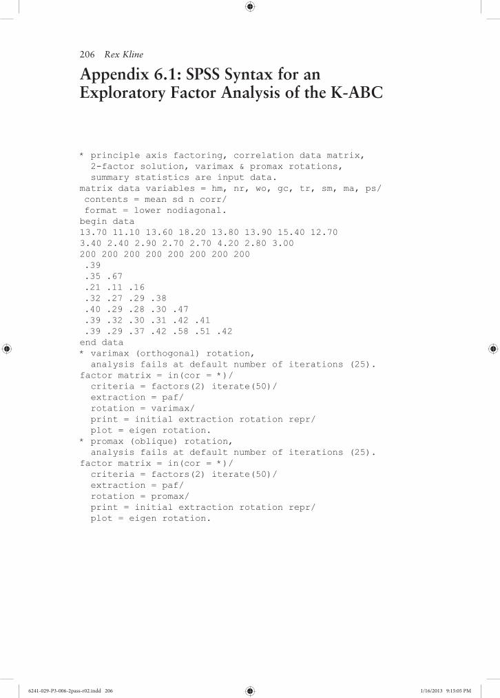
206 Rex Kline
Appendix 6.1: SPSS Syntax for an Exploratory Factor Analysis of the K-ABC
* principle axis factoring, correlation data matrix, 2-factor solution, varimax & promax rotations, summary statistics are input data.matrix data variables = hm, nr, wo, gc, tr, sm, ma, ps/ contents = mean sd n corr/ format = lower nodiagonal.begin data13.70 11.10 13.60 18.20 13.80 13.90 15.40 12.703.40 2.40 2.90 2.70 2.70 4.20 2.80 3.00200 200 200 200 200 200 200 200 .39 .35 .67 .21 .11 .16 .32 .27 .29 .38 .40 .29 .28 .30 .47 .39 .32 .30 .31 .42 .41 .39 .29 .37 .42 .58 .51 .42end data* varimax (orthogonal) rotation, analysis fails at default number of iterations (25).factor matrix = in(cor = *)/ criteria = factors(2) iterate(50)/ extraction = paf/ rotation = varimax/ print = initial extraction rotation repr/ plot = eigen rotation.* promax (oblique) rotation, analysis fails at default number of iterations (25).factor matrix = in(cor = *)/ criteria = factors(2) iterate(50)/ extraction = paf/ rotation = promax/ print = initial extraction rotation repr/ plot = eigen rotation.
6241-029-P3-006-2pass-r02.indd 2066241-029-P3-006-2pass-r02.indd 206 1/16/2013 9:15:05 PM1/16/2013 9:15:05 PM

Exploratory and Confi rmatory Factor Analysis 207
Appendix 6.2: Mplus Syntax for a Confi rmatory Factor Analysis of the K-ABC
title: 2-factor standard CFA model, ML estimation, covariance data matrixdata:! read summary statistics from external text fi le: fi le is “kabc.dat”; type is stdeviations correlation; Ngroups = 1; Nobservations = 200;variable: names are hm nr wo gc tr sm ma ps;analysis: type is general;model:! indicator-factor correspondence: Sequent by hm nr wo; Simult by gc tr sm ma ps;! Mplus automatically scales factors and specifi es! error terms and factor variances and covarianceoutput: sampstat modindices(all,0) residual stdyx; ! requests standardized solution, residuals, and ! all modifi cation indexes > 0
Contents of File “kabc.dat”
3.40 2.40 2.90 2.70 2.70 4.20 2.80 3.001.00 .39 1.00 .35 .67 1.00 .21 .11 .16 1.00 .32 .27 .29 .38 1.00 .40 .29 .28 .30 .47 1.00 .39 .32 .30 .31 .42 .41 1.00 .39 .29 .37 .42 .58 .51 .42 1.00
6241-029-P3-006-2pass-r02.indd 2076241-029-P3-006-2pass-r02.indd 207 1/16/2013 9:15:05 PM1/16/2013 9:15:05 PM