part iii count data - wu (wirtschaftsuniversität...

Count Data

Part III

Count Data

Count Data

Count Data

Count Data

Count data, in which there is no upper limit to the number ofcounts, usually fall into two types

I rates counts per unit of time/area/distance, etc

I contingency tables counts cross-classified by categoricalvariables

We will see that both of these types of count data can be modelledusing Poisson glms with a log link.

Count Data

Modelling Rates

Poisson Processes

Poisson Processes

Often counts are based on events that may be assumed to arisefrom a Poisson process, where

I counts are observed over fixed time interval

I probability of the event approximately proportional to lengthof time for small intervals of time

I for small intervals of time probability of > 1 event is neglibilecompared to probability of one event

I numbers of events in non-overlapping time intervals areindependent

Count Data

Modelling Rates

Poisson Processes

Examples include

I number of household burglaries in a city in a given year

I number of customers served by a saleperson in a given month

I number of train accidents in a given year

In such situations, the counts can be assumed to follow a Poissondistribution, say

Yi ∼ Poisson(λi)

Count Data

Modelling Rates

Poisson Processes

Rate Data

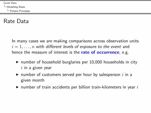
In many cases we are making comparisons across observation unitsi = 1, . . . , n with different levels of exposure to the event andhence the measure of interest is the rate of occurrence, e.g.

I number of household burglaries per 10,000 households in cityi in a given year

I number of customers served per hour by salesperson i in agiven month

I number of train accidents per billion train-kilometers in year i

Count Data

Modelling Rates

Poisson Processes

Since the counts are Poisson distributed, we would like to use aglm to model the expected rate, λi/ti, where ti is the exposure forunit i.

Typically explanatory variables have a multiplicative effect ratherthan an additive effect on the expected rate, therefore a suitablemodel is

log(λi/ti) = β0 +p∑r=1

xirβr

⇒ log(λi) = log(ti) + β0 +p∑r=1

xirβr

i.e. Poisson glm with the canonical log link.

This is known as a log-linear model.

Count Data

Modelling Rates

Poisson Processes

Offsets

The standardizing term log(ti) is an example of an offset: a termwith a fixed coefficient of 1.

Offsets are easily specified to glm, either using the offsetargument or using the offset function in the formula, e.g.offset(time).

If all the observations have the same exposure, the model does notneed an offset term and we can model log(λi) directly.

Count Data

Modelling Rates

Poisson Processes

Ship Damage Data

The ships data from the MASS package concern a type of damagecaused by waves to the forward section of cargo-carrying vessels.The variables are

I incidents number of damage incidents

I service aggregate months of service

I period period of operation : 1960-74, 75-79

I year year of construction: 1960-64, 65-69, 70-74, 75-79

I type type: ’”A”’ to ’”E”’

Here it makes sense to model the expected number of incidents peraggregate months of service.

Count Data

Modelling Rates

Poisson Processes

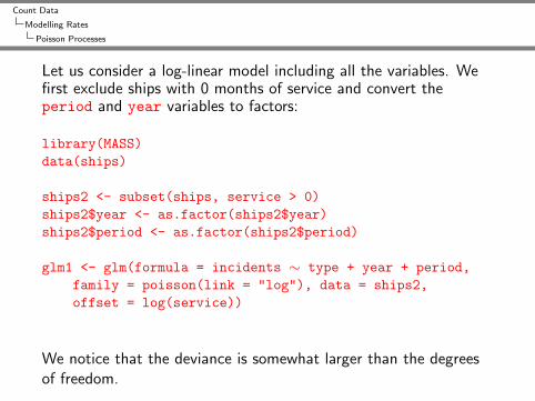
Let us consider a log-linear model including all the variables. Wefirst exclude ships with 0 months of service and convert theperiod and year variables to factors:

library(MASS)data(ships)

ships2 <- subset(ships, service > 0)ships2$year <- as.factor(ships2$year)ships2$period <- as.factor(ships2$period)

glm1 <- glm(formula = incidents ∼ type + year + period,family = poisson(link = "log"), data = ships2,offset = log(service))

We notice that the deviance is somewhat larger than the degreesof freedom.

Count Data

Modelling Rates

Overdispersion

Overdispersion

Lack of fit may be due to inadequate specification of the model,but another possibility when modelling discrete data isoverdispersion.

Under the Poisson or Binomial model, we have a fixedmean-variance relationship:

var(Yi) = V (µi)

Overdispersion occurs when

var(Yi) > V (µi)

This may occur due to correlated responses or variability betweenobservational units.

Count Data

Modelling Rates

Overdispersion

We can adjust for over-dispersion by estimating a dispersionparameter

var(Yi) = φV (µi)

This changes the assumed distribution of our response, to adistribution for which we do not have the full likelihood.

However the score equations in the IWLS

∂l

∂βj=

n∑i=1

ai(yi − µi)V (µi)

× xijg′(µi)

= 0

only require the variance function, so we can still obtain estimatesfor the parameters. Note the score equations do not depend on φ,so we will obtain the same estimates as if φ = 1.

Count Data

Modelling Rates

Overdispersion

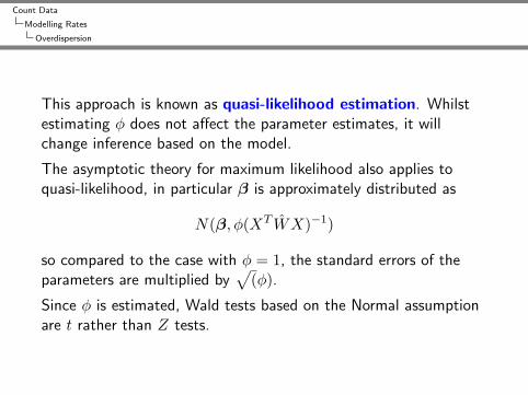
This approach is known as quasi-likelihood estimation. Whilstestimating φ does not affect the parameter estimates, it willchange inference based on the model.

The asymptotic theory for maximum likelihood also applies toquasi-likelihood, in particular β is approximately distributed as

N(β, φ(XT WX)−1)

so compared to the case with φ = 1, the standard errors of theparameters are multiplied by

√(φ).

Since φ is estimated, Wald tests based on the Normal assumptionare t rather than Z tests.

Count Data

Modelling Rates

Overdispersion

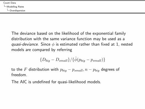
The deviance based on the likelihood of the exponential familydistribution with the same variance function may be used as aquasi-deviance. Since φ is estimated rather than fixed at 1, nestedmodels are compared by referring

{Dbig −Dsmall}/{φ(pbig − psmall)}

to the F distribution with pbig − psmall, n− pbig degrees offreedom.

The AIC is undefined for quasi-likelihood models.

Count Data

Modelling Rates

Overdispersion

In the Ships Damage data, it is likely that there is inter-shipvariability in accident-proneness. Therefore we might expect someover-dispersion.

We can switch to a quasi-likelihood estimation using thecorresponding quasi- family in R:

glm2 <- update(glm1, family = quasipoisson(link = "log"))

The dispersion parameter is estimated as 1.69, much larger thanthe value of 1 assumed under the Poisson model.

Count Data

Modelling Rates

Overdispersion

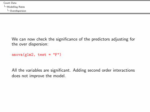
We can now check the significance of the predictors adjusting forthe over dispersion:

anova(glm2, test = "F")

All the variables are significant. Adding second order interactionsdoes not improve the model.

Count Data

Modelling Rates

Overdispersion

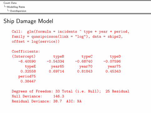
Ship Damage Model

Call: glm(formula = incidents ~ type + year + period,family = quasipoisson(link = "log"), data = ships2,offset = log(service))

Coefficients:(Intercept) typeB typeC typeD

-6.40590 -0.54334 -0.68740 -0.07596typeE year65 year70 year75

0.32558 0.69714 0.81843 0.45343period750.38447

Degrees of Freedom: 33 Total (i.e. Null); 25 ResidualNull Deviance: 146.3Residual Deviance: 38.7 AIC: NA

Count Data

Modelling Rates

Overdispersion

Intepretation of Ship Damage Model

We have the model

log(λtyp) = log(styp) + β0 + β1t + β2y + β3p

Consider ships of type C and E. We have

log(λEyp)− log(λCyp) = log(sEyp)− log(sCyp) + β1E − β1C

Since β1A = 0, we have

β1E − β1C = log(λEypsEyp

)− log

(λCypsCyp

)= log

(rEyprCyp

)So exp(β1E − β1C) is the ratio of the rates (expected number ofdamages per month in service)

Count Data

Modelling Rates

Overdispersion

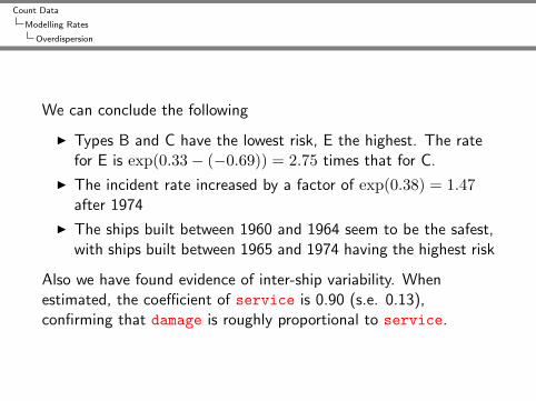
We can conclude the following

I Types B and C have the lowest risk, E the highest. The ratefor E is exp(0.33− (−0.69)) = 2.75 times that for C.

I The incident rate increased by a factor of exp(0.38) = 1.47after 1974

I The ships built between 1960 and 1964 seem to be the safest,with ships built between 1965 and 1974 having the highest risk

Also we have found evidence of inter-ship variability. Whenestimated, the coefficient of service is 0.90 (s.e. 0.13),confirming that damage is roughly proportional to service.

Count Data

Modelling Contingency Tables

Sampling Schemes

Contingency Tables

The counts in contingency tables could arise from differentsampling schemes.

It may be that the cell counts are realizations of independentPoisson processes, e.g. different groups of patients attending ahealth clinic during a fixed period of time. Thus we have countsnc, c = 1, . . . , C distributed as Poisson(µc).

More commonly, the cell counts may an observation of amultinomial response, e.g a fixed sample of patients is taken andcross-classified by cholesterol level and whether or not they hadheart disease. Thus we have a set of counts n1, . . . nC distributedas Multinomial(p1, . . . , pc, n).

Count Data


Sampling Schemes

It can be shown that if the cell counts are realizations ofindependent Poisson processes but the total count is fixed a priori,then the cell counts are Multinomial(µ1/n, . . . , µc/n, n).

Thus under either sampling scheme, the cell counts can bemodelled using a Poisson glm. In the multinomial case wecondition on the total count by including an intercept in the model.

We will consider models for contingency tables from the viewpointof multinomial sampling.

Count Data


Models for Two-way Tables

Independence ModelIf the two cross-classifying variables are independent, the jointprobabilities for the cells in that table are simply determined by themarginal probabilities:

P (X = i and Y = j) = P (X = i)P (Y = j)or pij = pipj

In terms of log expected frequencies we have

log(µij) = log(npij) = log n+ log(pipj)= log n+ log pi + log pj

i.e. a Poisson log-linear model. We represent this independencemodel as

log(µij) = λ0 + λXi + λYj

Count Data



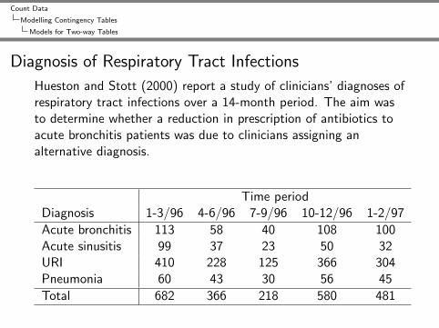
Diagnosis of Respiratory Tract Infections

Hueston and Stott (2000) report a study of clinicians’ diagnoses ofrespiratory tract infections over a 14-month period. The aim wasto determine whether a reduction in prescription of antibiotics toacute bronchitis patients was due to clinicians assigning analternative diagnosis.

Time periodDiagnosis 1-3/96 4-6/96 7-9/96 10-12/96 1-2/97

Acute bronchitis 113 58 40 108 100Acute sinusitis 99 37 23 50 32URI 410 228 125 366 304Pneumonia 60 43 30 56 45

Total 682 366 218 580 481

Count Data



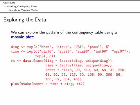
Exploring the Data

We can explore the pattern of the contingency table using amosaic plot:

diag <- rep(c("bron", "sinus", "URI", "pneu"), 5)time <- rep(c("win96", "spr96", "sum96", "aut96", "spr97"),

rep(4, 5))rt <- data.frame(diag = factor(diag, unique(diag)),

time = factor(time, unique(time)),count = c(113, 99, 410, 60, 58, 37, 228,43, 40, 23, 125, 30, 108, 50, 366, 56,100, 32, 304, 45))

plot(xtabs(count ∼ time + diag, rt))

Count Data



The pattern is similar to what would be given by an independencemodel.

We can see this by fitting this model and plotting a mosaic plot ofthe fitted counts

ind <- glm(count ∼ diag + time, poisson, rt)plot(xtabs(fitted(ind) ∼ time + diag, rt))

However the deviance shows that there is significant lack of fit (D= 29.59, d.f. = 12). Rejecting this model is equivalent to rejectinga null hypothesis of independence using a Pearson χ2 test.

Count Data



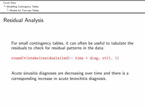
Residual Analysis

For small contingency tables, it can often be useful to tabulate theresiduals to check for residual patterns in the data:

round(t(xtabs(residuals(ind)∼ time + diag, rt)), 1)

Acute sinusitis diagnoses are decreasing over time and there is acorresponding increase in acute bronchitis diagnosis.

Count Data



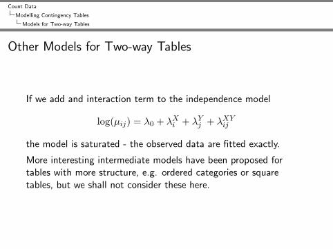
Other Models for Two-way Tables

If we add and interaction term to the independence model

log(µij) = λ0 + λXi + λYj + λXYij

the model is saturated - the observed data are fitted exactly.

More interesting intermediate models have been proposed fortables with more structure, e.g. ordered categories or squaretables, but we shall not consider these here.

Count Data


Models for Three-way Tables

Mutual Independence Model

If each pair of variables are independent, then

pijk = pipjpk

which is represented by the mutual independence model

log(µijk) = λ0 + λXi + λYj + λZk

This model is rarely interesting - we are more interested inassociations between the variables.

Count Data



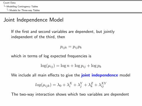
Joint Independence Model

If the first and second variables are dependent, but jointlyindependent of the third, then

pijk = pijpk

which in terms of log expected frequencies is

log(µij) = logn+ log pij + log pk

We include all main effects to give the joint independence model

log(µijk) = λ0 + λXi + λYj + λZk + λXYij

The two-way interaction shows which two variables are dependent

Count Data



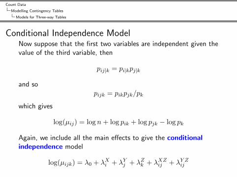
Conditional Independence ModelNow suppose that the first two variables are independent given thevalue of the third variable, then

pij|k = pi|kpj|k

and sopijk = pikpjk/pk

which gives

log(µij) = logn+ log pik + log pjk − log pk

Again, we include all the main effects to give the conditionalindependence model

log(µijk) = λ0 + λXi + λYj + λZk + λXZij + λY Zij

Count Data



Further Models

Including all two-way interactions results in the uniformassociation model, considered later.

All the models described so far are nested within the saturatedmodel, which includes the three-way interaction and all lower-orderterms.

A simple approach to identify the appropriate association model isto start with the saturated model and determine how the modelcan be simplified.

Count Data



Example: Drug Use

The following 2 x 2 x 2 table cross-classifies students according totheir alcohol, cigarette and drug use

Marijuana UseAlcohol Use Cigarette Use Yes No

Yes Yes 911 538No 44 456

No Yes 3 43No 2 279

Count Data



Modelling the Drugs Data

We don’t need to fit the saturated model since we know it has adeviance of zero on zero d.f. so we start with the uniformassociation model:

lab <- c("Y", "N")drugs <- data.frame(alcohol = gl(2, 4, 8, labels = lab),

cigarette = gl(2, 2, 8, labels = lab),marijuana = lab,count = c(911, 538, 44, 456, 3, 43, 2, 279))

unif <- glm(count ∼ . - alcohol:cigarette:marijuana,poisson, data = drugs)

summary(unif)

Count Data



The likelihood ratio test statistic to compare the uniformassociation model to the saturated model is simply the deviance ofthe uniform association model. So we can see that adding thethree-way interaction does not significantly improve the model.

It is clear that dropping any further terms from the model willsignificantly increase the deviance.

Count Data



Uniform Association Model

The uniform association model is so called because the odds ratiosbetween two variables are the same for any level of the thirdvariable. E.g. for any level of marijuana use i

odds of alcohol use|cigarette use

odds of alcohol use|no cigarette use=µY Y i/µNY iµY Ni/µNNi

= exp(λalc,cigY Y ) = exp(2.05) = 7.8

i.e. students who have smoked cigarettes have estimated odds ofalcohol use that are 7.8 times the estimated odds for students whohave not smoked cigarettes.

Count Data


Models for Higher Dimensional Tables

Higher Dimensional Tables

The same ideas extend to higher dimensional tables, althoughmodel-building and interpretation can be quite complex.

In the drug use example, students were also classified by sex andrace.

We use ftable to view the full data:

drugs2 <- read.table("drugs.txt", header = TRUE)ftable(xtabs(count ∼ sex + marijuana + alcohol +

cigarette + race, drugs2))

Count Data



Response and Explanatory Factors

Here sex and race are explanatory factors. We treat the marginaltotals of these factors as being fixed.

The minimal model must contain the interaction of all theexplantory factors.

Interactions between the response factors – here alcohol, cigaretteand marijuana use – and the explantory factors indicate interestingstructure.

Count Data



Model Building

We consider blocks of terms to determine the order of the model:

ind <- glm(count ∼ . + race:sex, poisson, data = drugs2)homog <- glm(count ∼ (.)^2, poisson, data = drugs2)ord3 <- glm(count ∼ (.)^3, poisson, data = drugs2)anova(ind, homog, ord3, test = "Chisq")

It seems we do not need to consider terms of higher order than 2.

Count Data



Now we try to simplify the homogeneous association model.

We can consider the effect of single deletions using drop1:

drop1(homog)homog <- update(homog, . ∼ . - sex:cigarette)

Dropping the race:cigarette interaction leads to the smallestincrease in deviance, so we drop this term.

Count Data



We continue dropping terms until no terms can be droppedwithout significantly increasing the deviance:

drop1(homog)homog <- update(homog, . ∼ . - race:sex)homog <- update(homog, . ∼ . - race:cigarette)homog <- update(homog, . ∼ . - race:marijuana)

The final model has seven two-way interactions, with a deviance of20.54 on 20 d.f.

Count Data



Association Graph

The final model can be represented by the association graph(shown on the board!)

Every path between cigarettes and {sex, race } involves avariable in {alcohol, marijuana}.Thus given the outcome on alcohol and marijuana use, cigaretteuse is independent of race and gender.

Count Data



Cigarette use can thus be safely summarised in a table collapsedover sex and race (proportion using cigarettes in each category):

Alcohol Marijuana UseUse Yes No

Yes 95% 54%No 60% 13%

Note here that the figure of 60% smoking in the ’marijuana butnot alcohol’ cell is based on only 5 cases and should therefore betreated with caution.

Count Data

Exercises

Exercises

1. The following data are from a cross-sectional study of 400patients with a form of skin cancer called malignant melanoma.

SiteTumour type Head & neck Trunk Extremities TotalHutchinson’s melanotic freckle 22 2 10 34Superficial spreading melanoma 16 54 115 185Nodular 19 33 73 125Indeterminate 11 17 28 56Total 68 106 226 400

Create a data.frame in R from these data.

Count Data

Exercises

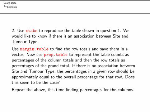
2. Use xtabs to reproduce the table shown in question 1. Wewould like to know if there is an association between Site andTumour Type.

Use margin.table to find the row totals and save them in avector. Now use prop.table to represent the table counts aspercentages of the column totals and then the row totals aspercentages of the grand total. If there is no association betweenSite and Tumour Type, the percentages in a given row should beapproximately equal to the overall percentage for that row. Doesthis seem to be the case?

Repeat the above, this time finding percentages for the columns.

Count Data

Exercises

3. An alternative way to view the data is to use a mosaic plot asseen in the lectures. Create this plot. Do Site and Tumour Typeseems to be independent?

4. We can test for independence using the conventionalchi-squared test. Under independence, the expected frequencies foreach cell can be calcuated from the marginal totals as follows:

eij = yi.y.j/n

These are compared to the observed values through the statistic

X2 =∑i

∑j

(yij − eij)2

eij

which under independence follows a χ2(i−1)(j−1) distribution.

Perform this test in R using chisq.test. What do you find?

Count Data

Exercises

5. Now fit the log-linear independence model to the data usingglm. Testing for a significant interaction term in the model isequivalent to testing the hypothesis of independence. Is theinteraction significant here?

Confirm that the sum of the squared pearson residuals from theindependence model is equal to the chi-squared statistic found inquestion 4.

Note the statistics in both tests are assumed to be approximatelyχ2

6, but they are different! We should obtain similar conclusions ifthe χ2 approximation is valid.

Count Data

Exercises

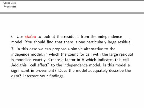
6. Use xtabs to look at the residuals from the independencemodel. You should find that there is one particularly large residual.

7. In this case we can propose a simple alternative to theindepende model, in which the count for cell with the large residualis modelled exactly. Create a factor in R which indicates this cell.Add this “cell effect” to the independence model. Is this model asignificant improvement? Does the model adequately describe thedata? Interpret your findings.

Count Data

Exercises

8. The data set “Long.txt” contains data on the productivity ofbiochemistry PhD students. The variables are as follows

I art Number of articles published by the student during lastthree years of PhD

I fem Gender: 1 if female, 0 if male

I mar Maritial status: 1 if married, 0 if not

I kid5 Number of children five years old or younger

I phd Prestige rating of PhD department

I ment Number of articles published by mentor during last threeyears

Read the dataset into R and attach the data frame.

Count Data

Exercises

9. Since the exposure of all students is fixed at three years, we canmodel the students’ article count directly, using a Poissonlog-linear model with no offset. Investigate the bivariaterelationships of log(art) with the other variables. Whichvariables does the article count appear to depend on?

10. Fit a Poisson log-linear model regressing art on the lineareffect of the other variables. Notice that the deviance is muchgreater than the degrees of freedom. Could this be due to a needfor second order terms?

Count Data

Exercises

11. Fit a quasi-Poisson model regressing art on the linear effect ofthe other variables. Do the data appear to be overdispersed?

12. Using a Poisson or quasi-Poisson model as you see fit, selectan appropriate model for art. Interpret your final model.

part iii count data - wu (wirtschaftsuniversität...

Documents