part iv nonadaptive fuzzy control - basu.ac.ir course in fuzzy... · the values of bz can be...
TRANSCRIPT
Part IV
Nonadaptive Fuzzy Control
When fuzzy systems are used as controllers, they are called fuzzy controllers. If fuzzy systems are used to model the process and controllers are designed based on the model, then the resulting controllers also are called fuzzy controllers. Therefore, fuzzy controllers are nonlinear controllers with a special structure. Fuzzy control has represented the most successful applications of fuzzy theory to practical problems.
Fuzzy control can be classified into nonadaptive fuzzy control and adaptive fuzzy control. In nonadaptive fuzzy control, the structure and parameters of the fuzzy controller are fixed and do not change during real-time operation. In adaptive fuzzy control, the structure orland parameters of the fuzzy controller change during real- time operation. Nonadaptive fuzzy control is simpler than adaptive fuzzy control, but requires more knowledge of the process model or heuristic rules. Adaptive fuzzy control, on the other hand, is more expensive to implement, but requires less information and may perform better. In this part (Chapters 16-22), we will study nonadaptive fuzzy control.
In Chapter 16, we will exam the trial-and-error approach to fuzzy controller design through two case studies: fuzzy control of a cement kiln and fuzzy control of a wastewater treatment process. In Chapters 17 and 18, stable and optimal fuzzy controllers for linear plants will be designed, respectively. In Chapters 19 and 20, fuzzy controllers for nonlinear plants will be developed in such a way that stability is guaranteed by using the ideas of sliding control and supervisory control. A fuzzy gain scheduling for PID controllers also will be studied in Chapter 20. In Chapter 21, both the plant and the controller will be modeled by the Takagi-Sugeno-Kang fuzzy systems and we will show how to choose the parameters such that the closed- loop system is guaranteed to be stable. Finally, Chapter 22 will introduce a few robustness indices for fuzzy control systems and show the basics of the hierarchical fuzzy systems.
Chapter 16
The Trial-and- Error Approach to Fuzzy Controller Design
16.1 Fuzzy Control Versus Conventional Control
Fuzzy control and conventional control have similarities and differences. They are similar in the following aspects:
They try to solve the same kind of problems, that is, control problems. There- fore, they must address the same issues that are common to any control prob- lem, for example, stability and performance.
The mathematical tools used to analyze the designed control systems are similar, because they are studying the same issues (stability, convergence, etc.) for the same kind of systems.
However, there is a fundamental difference between fuzzy control and conven- tional control:
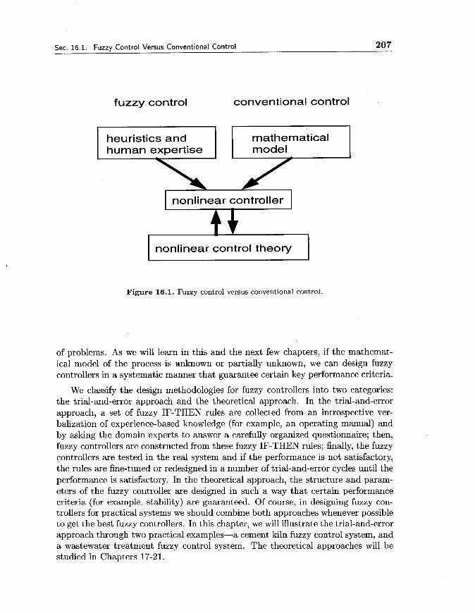
Conventional control starts with a mathematical model of the process and con- trollers are designed for the model; fuzzy control, on the other hand, starts with heuristics and human expertise (in terms of fuzzy IF-THEN rules) and controllers are designed by synthesizing these rules. That is, the information used to construct the two types of controllers are different; see Fig.lG.1. Ad- vanced fuzzy controllers can make use of both heuristics and mathematical models; see Chapter 24.
For many practical control problems (for example, industrial process control), it is difficult to obtain an accurate yet simple mathematical model, but there are experienced human experts who can provide heuristics and rule-of-thumb that are very useful for controlling the process. Fuzzy control is most useful for these kinds
Sec. 16.1. Fuzzy Control Versus Conventional Control 207
fuzzy control conventional control
heuristics and mathematical human expertise I I model
I nonlinear controller I
nonlinear control theory
Figure 16.1. Fuzzy control versus conventional control.
of problems. As we will learn in this and the next few chapters, if the mathemat- ical model of the process is unknown or partially unknown, we can design fuzzy controllers in a systematic manner that guarantee certain key performance criteria.
We classify the design methodologies for fuzzy controllers into two categories: the trial-and-error approach and the theoretical approach. In the trial-and-error approach, a set of fuzzy IF-THEN rules are collected from an introspective ver- balization of experience-based knowledge (for example, an operating manual) and by asking the domain experts to answer a carefully organized questionnaire; then, fuzzy controllers are constructed from these fuzzy IF-THEN rules; finally, the fuzzy controllers are tested in the real system and if the performance is not satisfactory, the rules are fine-tuned or redesigned in a number of trial-and-error cycles until the performance is satisfactory. In the theoretical approach, the structure and param- eters of the fuzzy controller are designed in such a way that certain performance criteria (for example, stability) are guaranteed. Of course, in designing fuzzy con- trollers for practical systems we should combine both approaches whenever possible to get the best fuzzy controllers. In this chapter, we will illustrate the trial-and-error approach through two practical examples-a cement kiln fuzzy control system, and a wastewater treatment fuzzy control system. The theoretical approaches will be studied in Chapters 17-21.

208 The Trial-and-Error Approach to Fuzzy Controller Design Ch. 16
16.2 The Trial-and-Error Approach to Fuzzy Controller Design
The trial-and-error approach to fuzzy controller design can be roughly summarized in the following three steps:
Step 1: Analyze the real system and choose state and control vari- ables. The state variables should characterize the key features of the system and the control variables should be able to influence the states of the system. The state variables are the inputs to the fuzzy controller and the control vari- ables are the outputs of the fuzzy controller. Essentially, this step defines the domain in which the fuzzy controller is going to operate.
Step 2. Derive fuzzy IF-THEN rules that relate the state variables with the control variables. The formulation of these rules can be achieved by means of two heuristic approaches. The most common approach involves an introspective verbalization of human expertise. A typical example of such verbalization is the operating manual for the cement kiln, which we will show in the next section. Another approach includes an interrogation of experienced experts or operators using a carefully organized questionnaire. In these ways, we can obtain a prototype of fuzzy control rules.
Step 3. Combine these derived fuzzy IF-THEN rules into a fuzzy system and test the closed-loop system with this fuzzy system as the controller. That is, run the closed-loop system with the fuzzy controller and if the performance is not satisfactory, fine-tune or redesign the fuzzy controller by trial and error and repeat the procedure until the performance is satisfactory.
We now show how to design fuzzy controllers for two practical systems using this approach-a cement kiln system and a wastewater treatment process.
16.3 Case Study I: Fuzzy Control of Cement Kiln
As we mentioned in Chapter 1, fuzzy control of cement kiln was one of the first successful applications of fuzzy control to full-scale industrial systems. In this sec- tion, we summarize the cement kiln fuzzy control system developed by Holmblad and Bsterguard [I9821 in the late '70s.
16.3.1 The Cement Kiln Process
Cement is manufactured by fine grinding of cement clinkers. The clinkers are pro- duced in the cement kiln by heating a mixture of limestone, clay, and sand com- ponents. For a wet process cement kiln, the raw material mixture is prepared in a slurry; see Fig.16.2. Then four processing stages follow. In the first stage, the water

Sec. 16.3. Case Studv I: Fuzzv Control of Cement Kiln 209
is driven off; this is called preheating. In the second stage, the raw mix is heated up and calcination (COz is driven off) takes place. The third stage comprises burning of the material a t a temperature of approximately 1430°C, where free lime (CaO) combines with the other components to form the clinker minerals. In the final stage, the clinkers are cooled by air.
coal from mill
m
burning
calcining slurry feeder
/ I preheating clinker zone W
I I I I cooler I I
xn burner pipe
I hot air
/ exhaust gas
Figure 16.2. The cement kiln process.
The kiln is a steel tube about 165 meters long and 5 meters in diameter. The kiln tube is mounted slightly inclined from horizontal and rotates 1-2 rev/min. The clinker production is a continuous process. The slurry is fed to the upper (back) end of the kiln, whereas heat is provided to the lower (front) end of the kiln; see Fig. 16.2. Due to the inclination and the rotation of the kiln tube, the material is transported slowly through the kiln in 3-4 hours and heated with hot gases. The hot combustion gases are pulled through the kiln by an exhaust gas fan and controlled by a damper that is in the upper end of the kiln as shown in Fig. 16.2.
Cement kilns exhibit time-varying nonlinear behavior and experience indicates that mathematical models for the process become either too simple to be of any practical value, or too comprehensive and needled into the specific process to possess

210 The Trial-and-Error Approach to Fuzzy Controller Design Ch. 16
any general applicability. However, humans can be trained and in a relatively short time become skilled kiln operators. Consequently, cement kilns are specially suitable for fuzzy control.
16.3.2 Fuzzy Controller Design for the Cement Kiln Process
First, we determine the state and control variables for this system. The state variables must characterize the main functioning of the cement kiln process and their values can be determined from sensory measurements. The control variables must be able to influence the values of the state variables. By analyzing the system, the following three state variables were chosen:
Temperature in the burning zone, denoted by BZ.
Oxygen percentage in the exhaust gases, denoted by OX.
Temperature at the back end of the kiln, denoted by BE.
The values of B Z can be obtained from the liter weight of clinkers, which is mea- sureable. The values of O X and B E are obtained from the exhaust gas analyzer shown at the back end of the kiln in Fig.16.2. Two control variables were chosen as follows:
Coal feed rate, denoted by CR.
Exhaust gas damper position, denoted by DP.
The exhaust gas damper position influences the air volume through the kiln. Each of the control variables influences the various stages of preheating, calcining, clinker formation and cooling with different delays and time constants ranging from minutes to hours. Looking at kiln control in general, we see that kiln speed and slurry fed rate can also be used as control variables, but as kilns are normally operated at constant production, the adjustment on feed rate and kiln speed are seldom used for regulatory control.
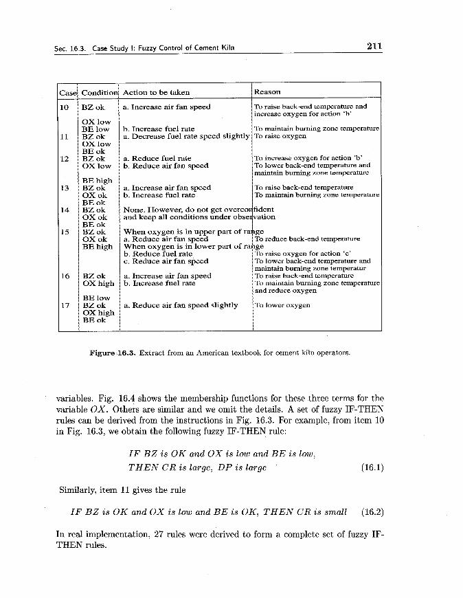
In the second step, we derive fuzzy IF-THEN rules relating the state variables BZ, OX and B E with the control variables CR and DP. We derive these rules from the operator's manual for cement kiln control. Fig. 16.3 illustrates an extract from an American textbook for cement kiln operators. This section describes how an operator must adjust fuel rate (coal feed rate), kiln speed, and air volumn through the kiln under various conditions characterized by the temperature in the burning zone BZ, oxygen percentages in the exhaust gases OX, and temperature at the back end of the kiln BE. We see that the conditions and control actions are described in qualitative terms such as "high," "ok," "low," "slightly increase," etc.
In order to convert the instructions in Fig. 16.3 into fuzzy IF-THEN rules, we first define membership functions for the terms "low," "ok," and "high" for different
Sec. 16.3. Case Study I: Fuzzy Control of Cement Kiln 211
Figure 16.3. Extract from an American textbook for cement kiln operators.
variables. Fig. 16.4 shows the membership functions for these three terms for the variable OX. Others are similar and we omit the details. A set of fuzzy IF-THEN rules can be derived from the instructions in Fig. 16.3. For example, from item 10 in Fig. 16.3, we obtain the following fuzzy IF-THEN rule:
Reason
I F BZ is O K and O X is low and BE is low,
THEN CR is large, DP is large
Action to be taken Case
Similarly, item 11 gives the rule
Condition
I F BZ is O K and OX is low and BE is OK, THEN CR is small (16.2)
10
11
In real implementation, 27 rules were derived to form a complete set of fuzzy IF- THEN rules.
BZ ok
OX low BE low BZ ok
a. Increase air fan speed
b. Increase fuel rate a. Decrease fuel rate speed slightly
OX low BE ok
To raise back-end temperature and increase oxygen for action 'b'
To maintain burning zone temperature To raise oxygen
To increase oxygen for action 'b' To lower back-end temperature and maintain burning zone temperature
12
13
14
15
BZ ok OX low
a. Reduce fuel rate b. Reduce air fan speed
BE high BZ ok OX ok BE ok BZ ok OX ok BE ok BZ ok OX ok BE high
a. Increase air fan speed b. Increase fuel rate
None. However, do not get ove and keep all conditions under o
When oxygen is in upper part of ralge a. Reduce air fan speed To reduce back-end temperature When oxygen is in lower part of ra ge
16
17
b. Reduce fuel rate c. Reduce air fan speed
a. Increase air fan speed b. Increase fuel rate
BZ ok OX high
BE low BZ ok OX high BE ok
To raise oxygen for action 'c' To lower back-end temperature and maintain burning zone temperatur To raise back-end temperature To maintain burning zone temperature
a. Reduce air fan speed slightly
and reduce oxygen
To lower oxygen

212 The Trial-and-Error Approach t o Fuzzy Controller Design Ch. 16
ok high
Figure 16.4. Membership functions for "low," "ok," and "high" for the variable OX.
16.3.3 Implementation
To develop a fuzzy control system for the real cement kiln process, it is not enough to have only one fuzzy controller. A number of fuzzy controllers were developed to operate in different modes. Specifically, the following two operating modes were considered:
The kiln is in a reasonably stable operation, measured by the kiln drive torque showing only small variations.
The kiln is running unstable, characterized by the kiln drive torque showing large and oscillating changes.
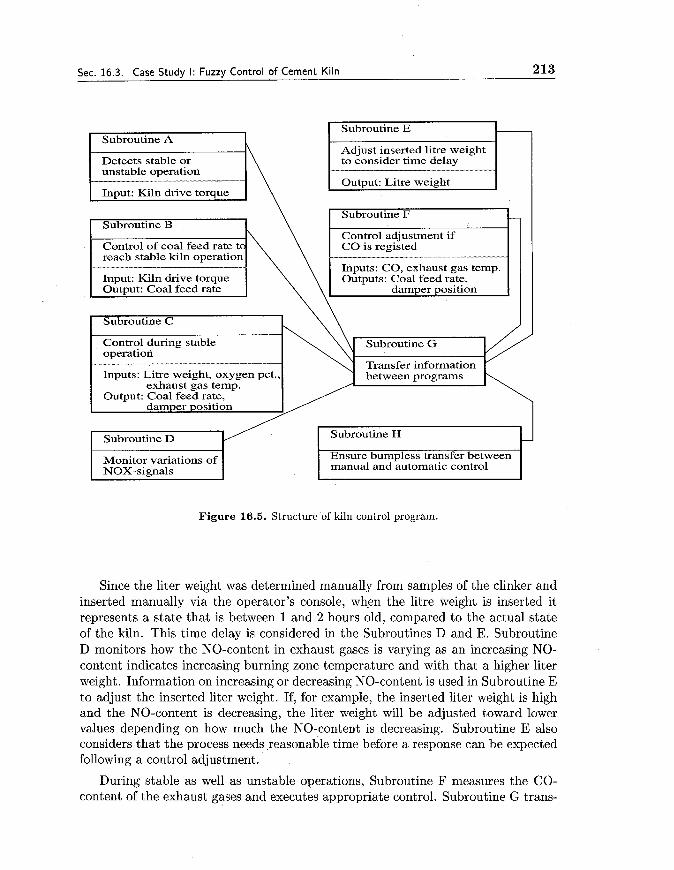
In the cement kiln fuzzy control system developed by Holmblad and Bsterguard [1982], eight operation subroutines were developed, in which each subroutine was represented by a fuzzy controller or some supporting operations. Fig. 16.5 shows these subroutines. Whether or not the kiln is in stable operation is determined by Subroutine A, which monitors the variations of the torque during a period of 8 hours. If the operation is unstable, control is taken over by Subroutine B, which adjusts only the amount of coal until the kiln is in stable operation again.
During stable operation, the desired values of the state variables were: liter weight about 1350g/Eiter, the oxygen about 1.8%, and the back-end temperature about 197OC. To approach and maintain this desired state, Subroutine C adjusts the coal feed rate and the exhaust gas damper position. This subroutine is the fuzzy controller described in the last subsection; it performs the main control actions.
Sec. 16.3. Case Study I: Fuzzy Control of Cement Kiln 213
Subroutine A
Detects stable or unstable operation
Input: Kiln drive torque
I Subroutine B I
Input: Kiln drive torque
Subroutine E
to consider time delay
Output: Litre weight I I Subroutine F I-
Control adjustment if CO is registed
Inputs: CO, exhaust gas temp. Outputs: Coal feed rate,
damner nosi ti on I I Subroutine C J I 7
Control during stable operation
Inputs: Litre weight, oxygen pct., exhaust gas temp.
Output: Coal feed rate, damper position
/
Subroutine G
Transfer information between programs C\
I Subroutine D Subroutine H
Monitor variations of NOX-signals
Ensure bumpless transfer between manual and automatic control
Figure 16.5. Structure of kiln control program.
Since the liter weight was determined manually from samples of the clinker and inserted manually via the operator's console, when the litre weight is inserted it represents a state that is between 1 and 2 hours old, compared to the actual state of the kiln. This time delay is considered in the Subroutines D and E. Subroutine D monitors how the NO-content in exhaust gases is varying as an increasing NO- content indicates increasing burning zone temperature and with that a higher liter weight. Information on increasing or decreasing NO-content is used in Subroutine E to adjust the inserted liter weight. If, for example, the inserted liter weight is high and the NO-content is decreasing, the liter weight will be adjusted toward lower values depending on how much the NO-content is decreasing. Subroutine E also considers that the process needs reasonable time before a response can be expected following a control adjustment.
During stable as well as unstable operations, Subroutine F measures the CO- content of the exhaust gases and executes appropriate control. Subroutine G trans-

214 The Trial-and-Error Approach to Fuzzy Controller Design Ch. 16
fers information between the subroutines and, finally, Subroutine H ensures that the human operator can perform bumpless transfers between manual and automatic kiln control.
16.4 Case Study II: Fuzzy Control of Wastewater Treatment Pro- cess
16.4.1 The Activated Sludge Wastewater Treatment Process
The activated sludge process is a commonly used method for treating sewage and wastewater. Fig. 16.6 shows the schematic of the system. The process (the part within the dotted lines) consists of an aeration tank and a clarifier. The wastewater entering the process is first mixed with the recycled sludge. Then, air is blown into the mixed liquor through diffusers placed along the base of the aeration tank. Complex biological and chemical reactions take place within the aeration tank, such that water and waste materials are separated. Finally, the processed mixed liquor enters the clarifier where the waste materials are settled out and the clear water is discharged.
air
I T
WS controller w desired' WWmS desired WS flow
Figure 16.6. Schematic of the activated sludge wastewater treatment process.

Sec. 16.4. Case Study II: Fuzzy Control of Wastewater Treatment Process 215
There are three low-level controllers as shown in Fig.16.6. The WW/RS con- troller regulates the ratio of the wastewater flow rate to the recycled sludge flow rate to the desired value. The objectives of this controller are to maintain a desirable ratio of substrate/organism concentrations and to manipulate the distribution of sludge between the aeration tank and the clarifier. The DO controller controls the air flow rate to maintain a desired dissolved oxygen level in the aeration tank. A higher dissolved oxygen level is necessary to oxidize nitrogen-bearing waste mate- rials (this is called nitrification). Finally, the WS controller is intended to regulate the total amount and average retention time of the sludge in both the aeration tank and the clarifier by controlling the waste sludge flow rate. Higher retention times of sludge are generally necessary to achieve nitrification.
Because the basic biological mechanism within the process is poorly understood, a usable mathematical model is difficult to obtain. In practice, the desired values of the WW/RS ratio, the DO level and the WS flow are set and adjusted by human operators. Our objective is to summarize the expertise of the human operators into a fuzzy system so that human operators can be released from the on-line operations. That is, we will design a fuzzy controller that gives the desired values of the WW/RS ratio, the DO level, and the WS flow. This fuzzy controller is therefore a higher level decision maker; the lower level direct control is performed by the WW/RS, DO, and WS controllers.
16.4.2 Design of the Fuzzy Controller
First, we specify the state and control variables. Clearly, we have the following three control variables:
A WW/RS: change in the desired WW/RS ratio.
A DO: change in the desired DO level.
A WS: change in the desired WS flow.
The state variables should characterize the essential features of the system. Since the overall objectives of the wastewater treatment process are to control the total amounts of biochemical oxygen and suspended solid materials in the output clear water to below certain levels, these two variables should be chosen as states. Ad- ditionally, the suspended solids in the mixed liquor leaving the aeration tank and in the recycled sludge also are important and should be chosen as state variables. Finally, the ammonia-nitrogen content of the output clear water ( N H 3 - N ) and the waste sludge flow rate also are chosen as state variables. In summary, we have the following six state variables:
TBO: the total amount of biochemical oxygen in the output clear water.
TSS: the total amount of suspended solid in the output clear water.

216 The Trial-and-Error Approach to Fuzzy Controller Design Ch. 16
MSS: the suspended solid in the mixed liquor leaving the aeration tank.
RSS: the suspended solid in the recycled sludge.
NH3-N: the ammonia-nitrogen content of the output clear water.
WSR: the waste sludge flow rate.
The next task is to derive fuzzy IF-THEN rules relating the state variables to the control variables. Based on the expertise of human operators, the 15 rules in Table 16.1 were proposed in Tong, Beck, and Latten [1980], where S, M, L, SN, LN, SP, LP, VS and NL correspond to fuzzy sets LLsmall," "medium," "large," "small negative," "large negative," "small positive," "large positive," "very small," and "not large," respectively. Rules 1-2 are resetting rules in that, if the process is in a satisfactory state but WSR is at abnormal levels, then the WSR is adjusted accordingly. Rules 3-6 deal with high NH3-N levels in the output water. Rules 7-8 cater for high output water solids. Rules 9-13 describe the required control actions if MSS is outside its normal range. Finally, Rules 14-15 deal with the problem of high biochemical oxygen in the output clear water.
The detailed operation of the system was described in Tong, Beck, and Latten [1980].
Table 16.1. Fuzzy IF-THEN rules for the wastewater treatment fuzzy controller.
RuleNo. 1 2 3 4 5 6 7 8 9 10 11 12 13 14 15
TBO TSS MSS RSS NH3-N WSR S S M M S S S S M M S L
S M S M S L S L
NL M NL L
L S
VS VS S L L
M S S L S S
A W W / R S A D O A WS SP SN
SP SN
LP LN
SP LP
LP SN LN
SP SN
SN LN
Sec. 16.5. Summary and Further Readings 217
16.5 Summary and Further Readings
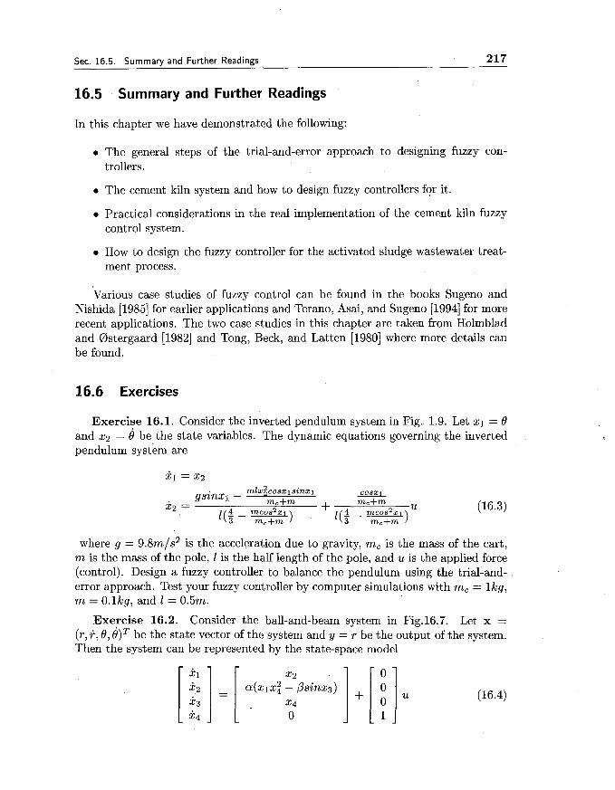
In this chapter we have demonstrated the following:
The general steps of the trial-and-error approach to designing fuzzy con- trollers.
The cement kiln system and how to design fuzzy controllers for it.
Practical considerations in the real implementation of the cement kiln fuzzy control system.
How to design the fuzzy controller for the activated sludge wastewater treat- ment process.
Various case studies of fuzzy control can be found in the books Sugeno and Nishida [I9851 for earlier applications and Terano, Asai, and Sugeno [I9941 for more recent applications. The two case studies in this chapter are taken from Holmblad and 0stergaard [I9821 and Tong, Beck, and Latten [I9801 where more details can be found.
16.6 Exercises
Exercise 16.1. Consider the inverted pendulum system in Fig. 1.9. Let xl = 8 and x2 = e be the state variables. The dynamic equations governing the inverted pendulum system are
where g = 9.8m/s2 is the acceleration due to gravity, mc is the mass of the cart, m is the mass of the pole, 1 is the half length of the pole, and u is the applied force (control). Design a fuzzy controller to balance the pendulum using the trial-and- error approach. Test your fuzzy controller by computer simulations with mc = lkg, m = O.lkg, and I = 0.5m.
Exercise 16.2. Consider the ball-and-beam system in Fig.16.7. Let x = (r, +, 8, 8)T be the state vector of the system and y = r be the output of the system. Then the system can be represented by the state-space model

218 The Trial-and-Error Approach to Fuzzy Controller Design Ch. 16
where the control u is the a,cceleration of 8, and a ,p are parameters. Design a fuzzy controller to control the ball to stay at the origin from a number of initial positions using the trial-and-error approach. Test your fuzzy controller by computer simulations with a = 0.7143 and /3 = 9.81.
Figure 16.7. The ball-and-beam system.
Exercise 16.3. Find more similarities and differences between fuzzy control and conventional control other than whose discussed in Section 16.1.
Exercise 16.4. Find an application of fuzzy control from the books Sugeno and Nishida [I9851 or Terano, Asai, and Sugeno [I9941 and describe the working principle of the fuzzy control system in some detail.

Chapter 17
Fuzzy Control of Linear Systems I: Stable Controllers
From Chapter 16 we see that the starting point of designing a fuzzy controller is to get a collection of fuzzy IF-THEN rules from human experts and operational manuals. That is, knowing the mathematical model of the process under control is not a necessary condition for designing fuzzy controllers. However, in order to analyze the designed closed-loop fuzzy control system theoretically, we must have a t least a rough model of the process. Additionally, if we want to design a fuzzy controller that guarantees some performance criterion, for example, globally exponential stability, then we must assume a mathematical model for the process, so that mathematical analysis can be done to establish the properties of the designed system. In this chapter, we consider the case where the process is a linear system and the controller is a fuzzy system. Our goal is to establish conditions on the fuzzy controller such that the closed-loop fuzzy control system is stable.
17.1 Stable Fuzzy Control of Single-Input-Single-Output Systems
For any control systems (including fuzzy control systems), stability is the most important requirement, because an unstable control system is typically useless and potentially dangerous. Conceptually, there are two classes of stability: Lyapunov stability and input-output stability. Within each class of stability, there are a number of specific stability concepts. We now briefly review these concepts.
For Lyapunov stability, let us consider the autonomous system
where x E Rn a d g(x) is a n x 1 vector function. Assume that g(0) = 0, thus x = 0 !f is an equilibriu point of the system.
Definition 17.1. (Lyapunov stability) The equilibrium point x = 0 is said to be stable if for any E > 0 there exists 6 > 0 such that I lx(0) 1 1 < S implies Ilx(t)ll < E

220 Fuzzy Control of Linear Systems I: Stable Controllers Ch. 17
for all t 2 0. It is said to be asymptotically stable if it is stable and additionally, there exists 6' > 0 such that 11x(0)11 < 6' implies x(t) -+ 0 as t -+ oo. Finally, the equilibrium point x = 0 is said to be exponentially stable if there exist positive numbers a, X and r such that
for all t 2 0 and llx(O)ll 5 T. If asymptotic or exponential stability holds for any initial state ~ ( 0 ) ~ then the equilibrium point x = 0 is said to be globally asymptotic or exponential stable, respectively.
For input-output stability, we consider any system that maps input u(t) E RT to output y(t) E Rm.
Definition 17.2. (Input-output stability) Let Lg be the set of all vector func- tions g(t) = (gl(t), ..., gn(t)lT : [O, W) -+ Rn such that 11g11, = (C:=' llgill~)'/2 < m7 where Ilgillp = (r l~ i ( t ) lpdt ) '~p~ P E [lyml and llgilla = S U P ~ ~ [ O , ~ ) Igi(t)l. A system with input u(t) E RT and output y(t) E Rm is said to be L,-stable if
u(t) E L i implies y(t) E L r (17.3)
where p E [0, oo]. In particular, a system is La-stable (or bounded-input-bounded- output stable) if u(t) E L&, implies y(t) E L g .
Now assume that the process under control is a single-input-single-output (SISO) time-invariant linear system represented by the following state variable model:
where u E R is the control, y E R is the output, and x E Rn is the state vector. A number of important concepts were introduced for this linear system.
Definition 17.3. (Controllability, Observability, and Positive Real) The system (17.4)-(17.5) is said to be controllable if
and observable if r c i
rank I r" = n
cAn-l
The transfer function of the system h(s) = c(s1-A)-'b is said to be strictly positive real if
inf Re[h(jw)] > 0 (17.8) w E R
We are now ready to apply some relevant results in control theory to fuzzy control systems.

Sec. 17.1. Stable Fuzzy Control of Single-Input-Single-Output Systems 221
17.1.1 Exponential Stability of Fuzzy Control Systems
Suppose that the control u(t) in the system (17.4)-(17.5) is a fuzzy system whose input is y(t), that is,
u(t) = - f [Y(t)l (17.9)
where f is a fuzzy system. Substituting (17.9) into (17.4)-(17.5), we obtain the closed-loop fuzzy control system that is shown in Fig.17.1. We now cite a famous result in control theory (its proof can be found in Vidyasagar [1993]).
process under control
Figure 17.1. Closed-loop fuzzy control system.
f(y
Proposition 17.1. Consider the closed-loop control system (17.4), (17.5), and (17.9), and suppose that (a) all eigenvalues of A lie in the open left half of the complex plane, (b) the system (17.4)-(17.5) is controllable and observable, and (c) the transfer function of the system (17.4)-(17.5) is strictly positive real. If the nonlinear function f satisfies f (0) = 0 and
c
then the equilibrium point x = 0 of the closed-loop system (17.4), (17.5) and (17.9) is globally exponentially stable.
fuzzy controller
Conditions (a)-(c) in Proposition 17.1 are imposed on the process under control, not on the controller f (y). They are strong conditions, essentially requiring that the open-loop system is stable and well-behaved. Conceptually, these systems are not difficult to control, thus the conditions on the fuzzy controller, f (0) = 0 and (17. lo), are not very strong. Proposition 17.1 guarantees that if we design a fuzzy controller

222 Fuzzy Control of Linear Systems I: Stable Controllers Ch. 17
f (y) that satisfies f (0) = 0 and (17.10), then the closed-loop system is globally exponentially stable, provided that the process under control is linear and satisfies conditions (a)-(c) in Proposition 17.1. We now design such a fuzzy controller.
Design of Stable Fuzzy Controller:
Step 1. Suppose that the output y ( t ) takes values in the interval U = [a, /I] c R. Define 2N+ 1 fuzzy sets A' in U that are normal, consistent, and complete with the triangular membership functions shown in Fig.17.2. That is, we use the N fuzzy sets A', ..., AN to cover the negative interval [a, 0), the other N fuzzy sets AN+ 2 , ..., A2N+1 to cover the positive interval (0, PI, and choose the center zN+l of fuzzy set AN+' a t zero.
Figure 17.2. Membership functions for the fuzzy con- troller.
Step 2. Consider the following 2N + 1 fuzzy IF-THEN rules:
IF y i s A', T H E N u is BZ (17.11)
where 1 = 1,2, ..., 2N + 1, and the centers fz of fuzzy sets BZ are chosen such that
< 0 f o r 1 = 1, ..., N = O f o r l = N + l 2 0 f o r l = N + 2 , ..., 2 N + 1
Step 3. Design the fuzzy controller from the 2N + 1 fuzzy IF-THEN rules (17.11) using product inference engine, singleton fuzzifier, and center average

Sec. 17.1. Stable Fuzzy Control of Single-Input-Single-Output Systems 223
defuzzifier; that is, the designed fuzzy controller is
where p ~ 1 (y) are shown in Fig. 17.2 and yZ satisfy (17.12).
We now prove that the fuzzy controller designed from the three steps above produces a stable closed-loop system.
Theorem 17.1. Consider the closed-loop fuzzy control system in Fig. 17.1. If the fuzzy controller u = - f (y) is designed through the above three steps (that is, u is given by (17.13)) and the process under control satisfies conditions (a)-(c) in Proposition 17.1, then the equilibrium point x = 0 of the closed-loop fuzzy control system is guaranteed to be globally exponentially stable.
Proof: From Proposition 17.1, we only need to prove f (0) = 0 and yf (y) 2 0 for all y E R. From (17.13) and Fig. 17.2 we have that f (0) = yNtl = 0. If y < 0, then from (17.13) and Fig. 17.2 we have
or f (y) = yll for some l1 E {1,2, ..., N). Since yll 5 0, yll+' I 0 and the member- ship functions are non-negative, we have f (y) < 0; therefore, y f (y) 2 0. Similarly, we can prove that yf (y) 2 0 if y > 0.
From the three steps of the design procedure we see that in designing the fuzzy controller f (y), we do not need to know the specific values of the process param- eters A, b and c. Also, there is much freedom in choosing the parameters of the fuzzy controller. Indeed, we only require that the yl's satisfy (17.12) and that the membership functions A1 are in the form shown in Fig.17.2. In Chapter 18, we will develop an approach to choosing the fuzzy controller parameters in an optimal fashion.
17.1.2 Input-Output Stability of Fuzzy Control Systems
The closed-loop fuzzy control system in Fig. 17.1 does not have an explicit input. In order to study input-output stability, we introduce an extra input and the system is shown in Fig. 17.3. We now cite a well-known result in control theory (its proof can be found in Vidyasagar [1993]).
Proposition 17.2. Consider the system in Fig.17.3 and suppose that the non- linear controller f (y) is globally Lipschitz continuous, that is,

224 Fuzzy Control of Linear Systems I: Stable Controllers Ch. 17
fuzzy controller
process under control
Figure 17.3. Closed-loop fuzzy control system with ex- ternal input.
4
for some constant a. If the open-loop unforced system x = AA~: is globally exponen- tially stable (or equivalently, the eigenvalues of A lie in the open left-half complex plane), then the forced closed-loop system in Fig. 17.3 is Lp-stable for all p E [l, m].
According to Proposition 17.2, if we can show that a designed fuzzy controller f (y) satisfies the Lipschitz condition (17.15), then the closed-loop fuzzy control system in Fig.17.3 is Lp-stable, provided that the eigenvalues of A lie in the open left-half complex plane. It is interesting to see whether the fuzzy controller (17.13) designed through the three steps in Subsection 17.1.1 satisfies the Lipschitz condi- tion (17.15). We first show that the fuzzy controller f (y) of (17.13) is a continuous, bounded, and piece-wise linear function, from which we conclude that it satisfies the Lipschitz condition.
f(y
Lemma 17.1, The fuzzy controller f (y) of (17.13) is continuous, bounded, and piece-wise linear.
4
Proof: Let 3' be the center of fuzzy set A' as shown in Fig.17.2 (1 = 1,2, ..., 2N+ 1). Since the membership functions in Fig. 17.2 are continuous, the f (y) of (17.13) is continuous. Since f (y) = y1 for y 5 zl, f (y) = y2N+1 for y 2 zaN+', and f (9) equals the weighted average of g1 and jj1+' for y E [zz , zl+l] (1 = 1 ,2 , ... ,2N), we conclude that the f (y) is bounded. To show that the f (y) is a piece-wise linear function, we partition the real line R into R = (-m, ~ ']u[z ' , 2 2 ] ~ . . u [ z ~ ~ , %2N+1 1 u [%2N+1, m). For y E (-m,5l] and y E [zZN+', m) , we have f (y) = 9' and f (y) = g2N+1, respectively, which are linear functions. For y E [21,~1+1] with some 1 E

Sec. 17.2. Stable Fuzzy Control o f Multi-Input-Multi-Output Systems 225
{1,2, ..., 2N), we have from Fig. 17.2 that
which is a linear function of y. Since f (y) is continuous, it is a piece-wise linear function.
Combining Lemma 17.1 and Proposition 17.2, we obtain the following theorem.
Theorem 17.2. Consider the closed-loop fuzzy control system in Fig.17.3. Suppose that the fuzzy controller f(y) is designed as in (17.13) and that all the eigenvalues of A lie in the open left-half complex plane. Then, the closed-loop fuzzy control system in Fig. 17.3 is L,-stable for all p E [0, oo].
Proof: Since a continuous, bounded, and piece-wise linear function satisfies the Lipschitz condition (17.15), this theorem follows from Proposition 17.2 and Lemma
17.2 Stable Fuzzy Control of Multi-Input-Multi-Output Systems
17.2.1 Exponential Stability
Consider the multi-input-multi-output (MIMO) linear system
where the input u(t) E Rm, the output y(t) E Rm, and the state x(t) E Rn. We assume that the number of input variables equals the number of output variables; this is called "squared" systems. In this case, the control u(t) = (ul(t), ..., ~ , ( t ) ) ~ consists of m fuzzy systems, that is,
where j = 1,2, ..., m, and fj[y(t)] are m-input-1-output fuzzy systems. The closed- loop fuzzy control system is still of the structure in Fig.17.1, except that the vector b is replaced by the matrix B, the vector c is replaced by the matrix C, and the scalar function f is replaced by the vector function f = (fl, ..., fm)T. For the MIMO system (17.17)-(17.18), controllability and observability are still defined by (17.6) and (17.7) with b changed to B and c changed to C. For strictly positive real, let

226 Fuzzv Control of Linear Systems I: Stable Controllers Ch. 17
H(s) = C(s I - A)-lB be the transfer matrix and H(s) is said to be strictly positive real if
inf X,i,[H(jw) + H* (jw)] > 0 w E R
(17.20)
where * denotes conjugate transpose, and Xmi,[H(jw) + H*(jw)] is the smallest eigenvalue of the matrix H(jw) + H* (jw).
As before, we first cite a result from control theory and then design a fuzzy controller that satisfies the conditions. The following proposition can be found in Vidyasagar [1993].
Proposition 17.3. Consider the closed-loop system (17.17)-(17.19), and sup- pose that: (a) all eigenvalues of A lie in the open left-half complex plane, (b) the system (17.17)-(17.18) is controllable and observable, and (c) the transfer matrix H(s) = C(s I - A)-lB is strictly positive real. If the control vector f (y) satisfies f (0) = 0 and
?lTf(y) 2 01 VY E Ern (17.21)
then the equilibrium point x = 0 of the closed-loop system (17.17)-(17.19) is globally exponentially stable.
Note that in order to satisfy (17.21), the m fuzzy systems { fl(y), ..., frn(y)) cannot be designed independently. We now design these m fuzzy systems in such a way that the resulting fuzzy controller f (y) = (fl(y), ..., frn(y))T satisfies (17.21).
Design of Stable Fuzzy Controller:
Step 1. Suppose that the output yi(t) takes values in the interval Ui = [ai, pi] c R, where i = 1,2, ..., m. Define 2Ni + 1 fuzzy sets Af" in Ui which are normal, consistent, and complete with the triangular membership functions shown in Fig. 17.2 (with the subscribe i added to all the variables).
Step 2. Consider m groups of fuzzy IF-THEN rules where the j'th group ( j = 1,2, ..., m) consists of the following nE1(2Ni + 1) rules:
IF yl i s A t and . . . and y, is A:, T H E N u i s B?""~ (17.22)
where li = 1,2 ,..., 2Ni + 1,i = 1,2, ..., m, and the center jj?""" of the fuzzy set ~ 1 ? "'1"
3 are chosen such that
where li for i = 1,2, ..., m with i # j can take any values from {1,2, ..., 2Ni+l).
Step 3. Design m fuzzy systems fj(y) each from the n L l ( 2 N i + 1) rules in (17.22) using product inference engine, singleton fuzzifier, and center average

Sec. 17.2. Stable Fuzzy Control of Multi-Input-Multi-Output Systems 227
defuzzifier; that is, the designed fuzzy controllers fj(y) are
where j = 1,2, ..., m.
We see from these three steps that as in the SISO case, we do not need to know the process parameters A, B and C in order to design the fuzzy controller; we only require that the membership functions are of the form in Fig.17.2 and the parameters jj?"'" satisfy (17.23). There is much freedom in choosing these parameters. We now show that the fuzzy controller u = (ul, ..., with u j designed as in (17.24) guarantees a stable closed-loop system.
Theorem 17.3. Consider the closed-loop fuzzy control system (17.17)-(17.19). If the fuzzy controller u = (ul, ..., = (- fl (y), ..., - f,(y))= is designed through the above three steps, (that is, u j = - fj(y) is given by (17.24)) and the process under control satisfies conditions (a)-(c) in Proposition 17.3, then the equilibrium point x = 0 of the closed-loop system is globally exponentially stable.
Proof: If we can show that f (0) = 0 and yTf (y) 2 0 for all y E Rm where f (y) = (fl(y), ..., fm(y))T, then this theorem follows from Proposition 17.3. From Fig.17.2, (17.23) and (17.24) we have that fj(0) = jj:N1+l)'..(Nm+l) = 0 for j = 1,2, ..., m. Since yTf(y) = ylfl(y) +...+y,fm(y), if we can show yjfj(y) > 0 for all yj E R and all j = 1,2, ..., m, then we have yT f (y) 2 0 for all y E Rm. If yj < 0, then from Fig. 17.2 we have that p I , (yJ) = 0 for lj = Nj + 2, ..., 2Nj + 1. Hence,
A" from (17.24) we have
2Ni+l.. . 2Nj-l+l Nj+l 2Nj+1+l 2Nm+l gl?...lm Cl1=l CljP1=l C l j= l Clj+l=l . . . Cim=l 3 ( n z 1 pA!i (yi))
f j ( ~ ) = 2N1+1 . . . 2Nm+1 Cl l=l Clj- l=l 2N'-1+1 gL:l ~;~:=l:l. zmzl ( n ~ , pA(, (Y~) )
(17.25) From (17.23) we have that jj?""" 5 O for Ij = 1,2, ..., Nj + 1, therefore fj(y) 5 0 and yj fj(y) 2 0. Similarly, we can prove that yjfj(y) > 0 if yj > 0.
17.2.2 Input-Output Stability
Consider again the closed-loop fuzzy control system (17.17)-(17-19). Similar to Proposition 17.2, we have the following result concerning the L,-stability of the control system.
Proposition 17.4 (Vidgasagar [1993]). Consider the closed-loop control system (17.17)-(17.19) and suppose that the open-loop unforced system x = Ax is globally exponentially stable. If the nonlinear controller f (y) = (fl (y), ..., f,(y))T
228 Fuzzy Control of Linear Systems I: Stable Controllers Ch. 17
is globally Lipschitz continuous, that is,
where a is a constant, then the closed-loop system (17.17)-(17.19) is Lp-stable for all p E [I, co].
Using the same arguments as for Lemma 17.1, we can prove that the fuzzy systems (17.24) are continuous, bounded, and piece-wise linear functions. Since a vector of continuous, bounded, and piece-wise linear functions satisfies the Lipschitz condition (17.26), we obtain the following result according to Proposition 17.4.
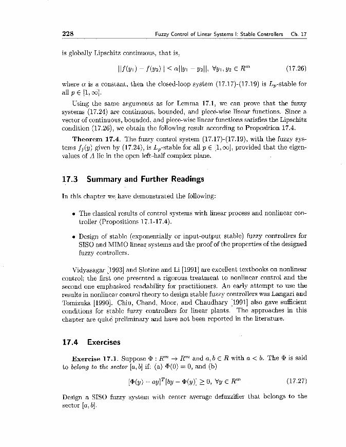
Theorem 17.4. The fuzzy control system (17.17)-(17.19), with the fuzzy sys- tems fj(y) given by (17.24), is Lp-stable for all p E [ l , m], provided that the eigen- values of A lie in the open left-half complex plane.
17.3 Summary and Further Readings
In this chapter we have demonstrated the following:
The classical results of control systems with linear process and nonlinear con- troller (Propositions 17.1-17.4).
Design of stable (exponentially or input-output stable) fuzzy controllers for SISO and MIMO linear systems and the proof of the properties of the designed fuzzy controllers.
Vidyasagar [I9931 and Slotine and Li [1991] are excellent textbooks on nonlinear control; the first one presented a rigorous treatment to nonlinear control and the second one emphasized readability for practitioners. An early attempt to use the results in nonlinear control theory to design stable fuzzy controllers was Langari and Tomizuka [1990]. Chiu, Chand, Moor, and Chaudhary [I9911 also gave sufficient conditions for stable fuzzy controllers for linear plants. The approaches in this chapter are quite preliminary and have not been reported in the literature.
17.4 Exercises
Exercise 17.1. Suppose @ : Rm -+ Rm and a, b E R with a < b. The @ is said to belong to the sector [a, b] if: (a) @(0) = 0, and (b)
Design a SISO fuzzy system with center average defuzzifier that belongs to the sector [a, b].

Sec. 17.4. Exercises 229
Exercise 17.2. Design a SISO fuzzy system with maximum defuzzifier that belongs to the sector [a, b].
Exercise 17.3. Design a 2-input-2-output fuzzy system (that is, two 2-input- 1-output fuzzy systems) with center average defuzzifier that belongs to the sector [a, bl.
Exercise 17.4. Design a 2-input-2-output fuzzy system with maximum defuzzi- fier that belongs to the sector [a, b].
Exercise 17.5. Show that the equilibrium point x = 0 of the system
is asymptotically stable but not exponentially stable. How about the system
Exercise 17.6. Suppose there exist constants a, b,c,r > 0, p > 1, and a continuous function V : Rn -i R such that
Prove that the equilibrium 0 is exponentially stable.
Exercise 17.7. Simulate the fuzzy controller designed in Section 17.1 for the linear system with the transfer function
Make your own choice of the fuzzy controller parameters that satisfy the condi- tions in the design steps. Plot the closed-loop system outputs with different initial conditions.

Chapter 18
Fuzzy Control of Linear Systems II: Optimal and
Robust Controllers
In Chapter 17 we gave conditions under which the closed-loop fuzzy control system is stable. Usually, we determine ranges for the fuzzy controller parameters such that stability is guaranteed if the parameters are in these ranges. We did not show how to choose the parameters within these ranges. In this chapter, we will first study how to determine the specific values of the fuzzy controller parameters such that certain performance criterion is optimized; that is, we first will consider the design of optimal fuzzy controllers for linear systems. This is a more difficult problem than designing stable-only fuzzy controllers. The approach in this chapter is very preliminary. In designing the optimal fuzzy controller, we must know the values of the plant parameters A, B and C, which are not required in designing the stable-only fuzzy controllers in Chapter 17.
The second topic in this chapter is robust fuzzy control of linear systems. This field is totally open and we will only show some very preliminary ideas of using the Small Gain Theorem to design robust fuzzy controllers.
18.1 Optimal Fuzzy Control
We first briefly review the Pontryagin Minimum Principle for solving the optimal control problem. Then, we constrain the controller to be a fuzzy system and de- velop a procedure for determining the fuzzy controller parameters such that the performance criterion is optimized.
Sec. 18.1. Optimal Fuzzy Control 231
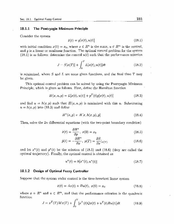
18.1.1 The Pontryagin Minimum Principle
Consider the system ~ ( t ) = g[x(t), u(t)l
with initial condition x(0) = xo, where x E Rn is the state, u 6 Rm is the control, and g is a linear or nonlinear function. The optimal control problem for the system (18.1) is as follows: determine the control u(t) such that the performance criterion
is minimized, where S and L are some given functions, and the final time T may be given.
This optimal control problem can be solved by using the Pontryagin Minimum Principle, which is given as follows. First, define the Hamilton function
and find u = h(x,p) such that H(x, u,p) is minimized with this u. Substituting u = h(x,p) into (18.3) and define
Then, solve the 2n differential equations (with the two-point boundary condition)
and let x*(t) and p*(t) be the solution of (18.5) and (18.6) (they are called the optimal trajectory). Finally, the optimal control is obtained as
u* (t) = h[x* (t), u* (t)] (18.7)
18.1.2 Design of Optimal Fuzzy Controller
Suppose that the system under control is the time-invariant linear system
where x E Rn and u E Rm, and that the performance criterion is the quadratic function
J = X~(T)MX(T) + [xT( t )~x( t ) + uT(t )~u( t ) ]d t IT (18.9)

232 Fuzzy Control of Linear Systems II: Optimal and Robust Controllers Ch. 18
where the matrices M E RnXn, Q E Rnxn and R E RmXm are symmetric and positive definite.
Now, assume that the controller u(t) is a fuzzy system in the form of (17.24) except that we change the system output y in (17.24) to the state x; that is, u(t) = ( ~ 1 , ..., with
We assume that the membership functions are fixed; they can be in the form shown in Fig.17.2 or other forms. Our task is to determine the parameters fj;"'" such that J of (18.9) is minimized.
Define the fuzzy basis functions b(x) = (bl (x), . .. , bN ( x ) ) ~ as
where li = 1,2 ,..., 2Ni + 1,1 = 1,2 ,..., N and N = nyz1(2Ni+ 1). Define the parameter matrix O E R m x N as
where O? E R1 consists of the N parameters jj?"'"" for li = 1,2, ..., 2Ni + 1 in the same ordering as bl(x) for 1 = 1,2, ..., N. Using these notations, we can rewrite the fuzzy controller u = (ul, ..., u , ) ~ = (-fi(x), ..., - f , ( ~ ) ) ~ as
To achieve maximum optimization, we assume that the parameter matrix O is time- vary, that is, O = O(t).
Substituting (18.13) into (18.8) and (18.9), we obtain the closed-loop system
and the performance criterion
Hence, the problem of designing the optimal fuzzy controller becomes the problem of determining the optimal O(t) such that J of (18.15) is minimized. Viewing the

Sec. 18.1. OotimaI Fuzzy Control 233
O ( t ) as the control u ( t ) in the Pontryagin Minimum Principle, we can determine the optimal O ( t ) from (18.3)-(18.7). Specifically, define the Hamilton function
H ( x , O , p ) = xT&x + b T ( x ) ~ T ~ ~ b ( x ) + p T [ A x + BOb(x)] (18.16)
From = 0 , that is,
d H -- - 2R@b(x) bT(x) + BTpbT ( x ) = 0 (18.17) d o
we obtain 1 o = --R-~B~~~~(x)[~(x)~~(x)]-~ 2
(18.18)
Substituting (18.18) into (18.16), we obtain
where a ( x ) is defined as
1 a ( x ) = - bT ( x ) [b(x) bT (x)]- 'b(x)
2 (18.20)
Using this H* in (18.5) and (18.6), we have
with initial condition x(0) = xo and p ( T ) = 2 M x ( T ) . Let x * ( t ) and p*(t) (t E [O,T]) be the solution of (18.21) and (18.22), then the optimal fuzzy controller parameters are
1 o* ( t ) = - - R-I BTp* ( t ) bT (x* ( t ) ) [b(x* ( t ) ) bT (x* (t))]-' 2
(18.23)
and the optimal fuzzy controller is
Note that the optimal fuzzy controller (18.24) is a state feedback controller with time-varying coefficients. The design procedure of this optimal fuzzy controller is now summarized as follows.

234 Fuzzy Control of Linear Systems II: Optimal and Robust Controllers Ch. 18
Design of the Optimal Fuzzy Controller:
Step 1. Specify the membership functions p l i (xi) to cover the state space, A i
where li = 1,2, ..., 2Ni + 1 and i = 1,2, ..., n. We may not choose the member- ship functions as in Fig. 17.2 because the function a(x) with these member- ship functions is not differentiable (we need % in (18.22)). We may choose pAli (xi) to be the Gaussian functions.
Step 2. Compute the fuzzy basis functions bl(x) from (18.11) and the function a(%) from (18.20). Compute the derivative v. Step 3. Solve the two-point boundary differential equations (18.21) and (18.22) and let the solution be x*(t) and p*(t), t E [0, TI. Compute O*(t) for t E [0, T] according to (18.23).
Step 4. The optimal fuzzy controller is obtained as (18.24)
Note that Steps 1-3 are off-line operations; that is, we first compute O*(t) fol- lowing Steps 1-3 and store the O* (t) for t E [0, TI in the computer, then in on-line operation we simply substitute the stored O*(t) into (18.24) to obtain the optimal fuzzy controller.
The most difficult part in designing this optimal fuzzy controller is to solve the two-point boundary differential equations (18.21) and (18.22). Since these differen- tial equations are nonlinear, numerical integration is usually used to solve them.
18.1.3 Application to the Ball-and-Beam System
Consider the ball-and-beam system in Fig. 16.7, with the state-space model given by (16.4)- (16.5). Since the ball-and-beam system is nonlinear, to apply our optimal fuzzy controller we have to linearize it around the equilibrium point x = 0. The linearized system is in the form of (18.8) with
We now design an optimal fuzzy controller for the linearized ball-and-beam system, and apply the designed controller to the original nonlinear system (16.4)- (16.5). We choose M = O , Q = I , R = I , T = 30, and Ni = 2 for i = 1,2,3,4. The membership functions p l i (xi) are chosen as
Ai
Sec. 18.2. Robust Fuzzy Control 235
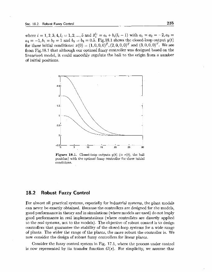
where i = 1,2,3,4, li = 1,2, ..., 5 and %$i = ai + bi(li - 1) with a1 = a2 = -2, as = a4 = -1, bl = b2 = 1 and bg = b4 = 0.5. Fig.18.1 shows the closed-loop output y(t) for three initial conditions: 4 0 ) = (1,0,0,0)*, ( 2 , 0 , 0 , 0 ) ~ and (3,0,0,0)*. We see from Fig.18.1 that although our optimal fuzzy controller was designed based on the linearized model, it could smoothly regulate the ball to the origin from a number of initial positions.
Figure 18.1. Closed-loop outputs y ( t ) (= r ( t ) , the ball position) with the optimal fuzzy controller for three initial conditions.
18.2 Robust Fuzzy Control
For almost all practical systems, especially for industrial systems, the plant models can never be exactly obtained. Because the controllers are designed for the models, good performance in theory and in simulations (where models are used) do not imply good performance in real implementations (where controllers are directly applied to the real systems, not to the models). The objective of robust control is to design controllers that guarantee the stability of the closed-loop systems for a wide range of plants. The wider the range of the plants, the more robust the controller is. We now consider the design of robust fuzzy controllers for linear plants.
Consider the fuzzy control system in Fig. 17.1, where the process under control is now represented by its transfer function G(s). For simplicity, we assume that

236 Fuzzy Control of Linear Systems II: Optimal and Robust Controllers Ch. 18
G(s) is a SISO system. Define
and 0, = {G(s) : Y(G) F a )
Clearly, the larger the a, the more plants in 0,. The objective of robust fuzzy, control is to design a fuzzy controller that stabilizes all the plants in R, while allowing the R, to be as large as possible. This is intuitively appealing because the larger the R,, the more plants the fuzzy controller can stabilize, which means that the fuzzy controller is more robust.
To achieve the objective, the key mathematical tool is the famous Small Gain Theorem (Vidyasagar [1993]). To understand this theorem, we must first introduce the concept of the gain of a nonlinear mapping.
Definition 18.1. Let f : R -+ R satisfy (f (x)l 2 y(x( for some constant y and all x E R. Then the gain off is defined as
The Small Gain Theorem is now stated as follows.
Small Gain Theorem. Suppose that the linear plant G(s) is stable and the nonlinear mapping f (y) is bounded for bounded input. Then the closed-loop system in Fig. 17.1 (with the process under control represented by G(s)) is stable if
F'rom (18.30) we see that a smaller y ( f ) will permit a larger y (G), and according to (18.27)-(18.28) a larger y(G) means a larger set R, of plants that the controller f (y) can stabilize. Therefore, for the purpose of robust control, we should choose y(f) as small as possible. The extreme case is f = 0, which means no control at all; this is impractical because feedback control is required to improve performance. Since the most commonly used fuzzy controller is a weighted average of the yl's (the centers of the THEN part membership functions), our recommendation for designing robust fuzzy controllers is the following: design the fuzzy controller using any method in Chapters 16-26, but try to use smaller yl's in the design.
Robust fuzzy control is an open field and much work remains to be done.
18.3 Summary and Further Readings
In this chapter we have demonstrated the following:
The Pontryagin Minimum Principle for solving the optimal control problem.

Sec. 18.4. Exercises ' 237
How to use the Pontryagin Minimum Principle to design the optimal fuzzy controller for linear plants.
The Small Gain Theorem and the basic idea of designing robust fuzzy con- trollers.
Good textbooks on optimal control are abundant in the literature, for example Anderson and Moore [I9901 and Bryson and Ho [1975]. A good book on robust control is Green and Limebeer [1995].
18.4 Exercises
Exercise 18.1. A simplified model of the linear motion of an automobile is j: = u, where x(t) is the vehicle velocity and u(t) is the acceleration or deceleration. The car is initially moving at xo mls. Using the Pontryagin Minimum Principle to design an optimal u(t) which brings the velocity x(tf) to zero in minimum time t f . Assume that acceleration and braking limitations require lu(t)l < M for all t, where M is a constant.
Exercise 18.2. Use the Pontryagin Minimum Principle to solve the optimiza- tion problems:
(a) X I = x2, x2 = U, XI (0) = 1, x2(0) = 1, XI (2) = 0,22(2) = 0, minimize J = u2(t)dt.
(b) 5 = u, x(0) = 0, x(1) = 1, minimize J = St (s2 + u2)dt.
Exercise 18.3. Derive the detailed formulas of the differential equations (18.21)- (18.22) for the example in Subsection 18.1.3. (You may or may not write out the details of q.)
Exercise 18.4. Design a fuzzy system f (a) with center average defuzdfier on U = [-I, 11 with at least five rules such that: (a) f (0) = 0, and (b) y(f) = 1, where the R in (18.29) is changed to U .
Exercise 18.5. Design a fuzzy system f (x) with maximum defuzzifier on U = [-I, I] with at least five rules such that: (a) f (0) = 0, and (b) y(f) = 1, where the R in (18.29) is changed to U .
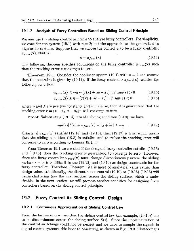
Chapter 19
Fuzzy Control of Nonlinear Systems I: Sliding Control
Sliding control is a powerful approach to controlling nonlinear and uncertain sys- tems. It is a robust control method and can be applied in the presence of model uncertainties and parameter disturbances, provided that the bounds of these un- certainties and disturbances are known. A careful comparison of sliding control and fuzzy control shows that their operations are similar in many cases. In this chapter, we will explore the relationship between fuzzy control and sliding control, and design fuzzy controllers based on sliding control principles.
19.1 Fuzzy Control As Sliding Control: Analysis
19.1.1 Basic Principles of Sliding Control
Consider the SISO nonlinear system
where u E R is the control input, z E R is the output, and x = (x, 2 , ..., x(n-l))T E Rn is the state vector. In (19.1), the function f (x) is not exactly known, but the uncertainty of f (x) is bounded by a known function of x; that is,
and lAf (x)l i F(x)
where A f (x) is unknown but f (x) and F(x) are known. The control objective is to determine a feedback control u = u(x) such that the state x of the closed-loop system will follow the desired state xd = (xd, kd, ..., x p - ' ) ) ~ ; that is, the tracking error
- e(n-l))T e = x - xd = (e, el ..., (19.4)

Sec. 19.1. Fuzzy Control As Sliding Control: Analysis 239
should converge to zero, where e = x - xd.
The basic idea of sliding control is as follows. Define a scalar function
where X is a positive constant. Then,
defines a time-varying surface S(t) in the state space Rn. For example, if n = 2 then the surface S(t) is
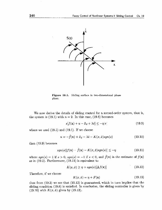
which is a straight line in the x - x phase plane, as shown in Fig. 19.1. Since id and xd are usually time-varying functions, the S(t) is also time-varying. If the initial state x(0) equals the initial desired state xd(0), that is, if e(0) = 0, then from (19.5) and (19.6) we see that if the state vector x remains on the surface S(t) for all t 2 0, we will have e(t) = 0 for all t 2 0. Indeed, s(x, t) = 0 represents a linear differential equation whose unique solution is e(t) = 0 for the initial condition e(0) = 0. Thus, our tracking control problem is equivalent to keeping the scalar function s(x, t) at zero. To achieve this goal, we can choose the control u such that
if the state is outside of S(t), where is a positive constant. (19.8) is called the sliding condition; it guarantees that I s(x, t) 1 will decrease if x is not on the surface S(t), that is, the state trajectory will move towards the surface S(t) , as illustrated in Fig. 19.1. The surface S(t) is referred to as the sliding surface, the system on the surface is in the sliding mode, and the control that guarantees (19.8) is called sliding mode control or sliding control. To summarize the discussions above, we have the following lemma.
Lemma 19.1. Consider the nonlinear system (19.1) and let s(x, t) be defined as in (19.5). If we can design a controller u such that the sliding condition (19.8) is satisfied, then:
(a) The state will reach the sliding surface S(t) within finite time.
(b) Once the state is on the sliding surface, it will remain there.
(c) If the state remains on the sliding surface, the tracking error e(t) will converge to zero.
Therefore, our goal is to design a controller u such that the closed-loop system satisfies the sliding condition (19.8).
240 Fuzzv Control of Nonlinear Svstems I: Sliding Control Ch. 19
Figure 19.1. Sliding surface in two-dimensional phase plane.
We now derive the details of sliding control for a second-order system, that is, the system is (19.1) with n = 2. In this case, (19.8) becomes
s [ f (x) + u - xd + Xe] 5 - 7 7 1 ~ 1 (19.9)
where we used (19.5) and (19.1). If we choose
then (19.9) becomes
where sgn(s) = 1 if s > 0, sgn(s) = -1 if s < 0, and f(x) is the estimate of f (x) as in (19.2). Furthermore, (19.11) is equivalent to
Therefore, if we choose K(x ,x) = r]+ F (x )
then from (19.3) we see that (19.12) is guaranteed, which in turn implies that the sliding condition (19.8) is satisfied. In conclusion, the sliding controller is given by (19.10) with K(z ,x) given by (19.13).
Sec. 19.2. Fuzzy Control As Sliding Control: Design 241
19.1.2 Analysis of Fuzzy Controllers Based on Sliding Control Principle
We now use the sliding control principle to analyze fuzzy controllers. For simplicity, we consider the system (19.1) with n = 2; but the approach can be generalized to high-order systems. Suppose that we choose the control u to be a fuzzy controller fuzz ( 4 , that is,
u = up UZZ(X) (19.14)
The following theorem specifies conditions on the fuzzy controller ufu,,(x) such that the tracking error e converges to zero.
Theorem 19.1. Consider the nonlinear system (19.1) with n = 2 and assume that the control u is given by (19.14). If the fuzzy controller ufUzz(x) satisfies the following condition:
where 7 and X are positive constants and s = B + Xe, then it is guaranteed that the tracking error e = (x - xd, x - kd)T will converge to zero.
Proof: Substituting (19.14) into the sliding condition (19.9), we have
Clearly, if up,,, (x) satisfies (19.15) and (19.16), then (19.17) is true, which means that the sliding condition (19.8) is satisfied and therefore the tracking error will converge to zero according to Lemma 19.1.
From Theorem 19.1 we see that if the designed fuzzy controller satisfies (19.15) and (19.16), then the tracking error is guaranteed to converge to zero. However, since the fuzzy controller uf,,, (x) must change discontinuously across the sliding surface s = 0, it is difficult to use (19.15) and (19.16) as design constraints for the fuzzy controller. Therefore, Theorem 19.1 is more of analytical value rather than design value. Additionally, the discontinuous control (19.10) or (19.15)-(19.16) will cause chattering (see the next section) across the sliding surface, which is unde- sirable. In the next section, we will propose another condition for designing fuzzy controllers based on the sliding control principle.
19.2 Fuzzy Control As Sliding Control: Design
19.2.1 Continuous Approximation of Sliding Control Law
From the last section we see that the sliding control law (for example, (19.10)) has to be discontinuous across the sliding surface S(t). Since the implementation of the control switchings could not be perfect and we have to sample the signals in digital control systems, this leads to chattering, as shown in Fig. 19.2. Chattering is
242 Fuzzy Control of Nonlinear Systems I: Sliding Control Ch. 19
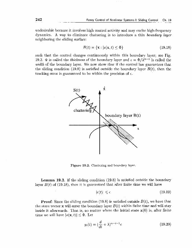
undesirable because it involves high control activity and may excite high-frequency dynamics. A way to eliminate chattering is to introduce a thin boundary layer neighboring the sliding surface:
such that the control changes continuously within this boundary layer; see Fig. 19.2. cP is called the thickness of the boundary layer and E = @/An-l is called the width of the boundary layer. We now show that if the control law guarantees that the sliding condition (19.8) is satisfied outside the boundary layer B(t), then the tracking error is guaranteed to be within the precision of 6 .
Figure 19.2. Chattering and boundary layer.
Lemma 19.2. If the sliding condition (19.8) is satisfied outside the boundary layer B(t) of (19.18), then it is guaranteed that after finite time we will have
Proof: Since the sliding condition (19.8) is satisfied outside B(t), we have that the state vector x will enter the boundary layer B(t) within finite time and will stay inside it afterwards. That is, no matter where the initial state x(0) is, after finite time we will have js(x, t ) 1 5 cP. Let
Sec. 19.2. Fuzzy Control As Sliding Control: Design 243
so we have
and d
~ i ( t ) = (;ii + N ~ i + l ( t )
for i = 0,1, ..., n - 2. Hence,
When i = 0, we have from (19.24), (19.21) and Is(x,t)l 5 + that
When i = 1, we have
Continuing this process until i = n - 2, we have
which is (19.19).
Lemma 19.2 shows that if we are willing to sacrifice precision, that is, from perfect tracking e(t) = 0 to tracking within precision le(t)l 5 c, the requirement for control law is reduced from satisfying the sliding condition (19.8) all the time to satisfying the sliding condition only when x(t) is outside of the boundary layer B(t). Consequently, we are able to design a smooth controller that does not need to switch discontinuously across the sliding surface. Specifically, for the second-order system, we change the control law (19.10) to

244 Fuzzy Control of Nonlinear Systems I: Sliding Control Ch. 19
where the saturation function sat(s/@) is defined as
Clearly, if the state is outside of the boundary layer, that is, if Is/@/ > 1, then sat(s/@) = sgn(s) and thus the control law (19.28) is equivalent to the control law (19.10). Therefore, the control law (19.28) with K(x , x) given by (19.13) guarantees that the sliding condition (19.8) is satisfied outside the boundary layer B(t). The control law (19.28) is a smooth control law and does not need to switch discontin- uously across the sliding surface.
19.2.2 Design of Fuzzy Controller Based on the Smooth Sliding Control Law
From the last subsection we see that if we design a fuzzy controller according to (19.28), then the tracking error is guaranteed to satisfy (19.19) within finite time. For a given precision E, we can choose @ and X such that E = @/An-'; that is, we can specify the design parameters @ and X such that the tracking error converges to any precision band le(t)l 5 E. Since the control u of (19.28) is a smooth function of x and x, we can design a fuzzy controller to approximate the u of (19.28). From the last subsection, we have the following theorem.
Theorem 19.2. Consider the nonlinear system (19.1) with n = 2 and assume that the control u is a fuzzy controller uf,,, If the fuzzy controller is designed as
ufU,, (x) = -f^(x) + xd - Xi: - [ r ] + F(x)]sat(s/@) (19.30)
then after finite time the tracking error e(t) = x(t) - xd(t) will satisfy (19.19).
Proof: Since the fuzzy controller (19.30) satisfies the sliding condition (19.8) when the state is outside of the boundary layer B(t), this theorem follows from Lemma 19.2.
Our task now is to design a fuzzy controller that approximates the right-hand side of (19.30). Since all the functions in the right-hand side of (19.30) are known, we can compute the values of the right-hand side of (19.30) at some regular points in the phase plane and design the fuzzy controller according to the methods in Chapters 10 and 11. Specifically, we have the following design method.
Design of the Fuzzy Controller:
Step 1. Determine the domains of interest for e and e; that is, determine the intervals [a l ,p l ] and [az,Pz] such that e = (e,e)T E U = [al ,Pl] x [az,Pz].
Step 2. Let g(e, i:) = -f^(x) + xd - Xk - [ r ] + F(x)]sat(s/@) and view this g(e, k ) as the g in (10.9). Design the fuzzy controller through the three steps in Sections 10.2 or 11.1; that is, the designed fuzzy controller is the fuzzy system (10.10).

Sec. 19.2. Fuzzv Control As Sliding Control: Design 245
The approximation accuracy of this designed fuzzy controller to the ideal fuzzy controller uf,,,(x) of (19.30) is given by Theorems 10.1 or 11.1. As we see from these theorems that if we sufficiently sample the domains of interest, the approxi- mation error can be as small as desired.
Example 19.1. Consider the first-order nonlinear system
l - e - " ( t ) where the nonlinear function f (x) = is assumed to be unknown. Our task is to design a fuzzy controller based on the smooth sliding control law such that the x(t) converges to zero.
Since
Z e - " ( t ) wechoose f(x) = l , A f ( z ) = m, and F(x) = 2, so that lAf(x)l 5 F(z) . For this example, xd = 0, e = x - 0 = z , s = e = x, and the sliding condition (19.8) becomes
~ ( f + U) I -171x1 (19.33)
Hence, the sliding control law is
where K(x) = + F(x) = + 2. Fig. 19.3 shows the closed-loop state x(t) using this sliding controller for four initial conditions, where we chose q = 0.1 and the sampling rate equal to 0.02s. We see that chattering occurred.
The smooth sliding controller is
usm(x) = - f (x) - K(x)sat(x/@) (19.35)
Viewing this u,,(x) as the g(x) in (10.9), we designed a fuzzy controller following the three steps in Section 11.1 (this is a one-dimensional system, a special case of the system in Section 11.1), where we chose @ = 0.2, U = [-2,2], N = 9, and the ej's to be uniformly distributed over [-2,2]. Fig.19.4 shows the closed-loop x(t) with this fuzzy controller for the same initial conditions as in Fig. 19.3. Comparing Figs.19.4 with 19.3, we see that chattering disappeared, but a steady tracking error appeared; this is as expected: chattering was smoothed out with the sacrifice of precision.

246 Fuzzv Control of Nonlinear Svstems I: Sliding Control ' Ch. 19
Figure 19.3. Closed-loop state x ( t ) for the nonlinear sys- tem (19.31) with the sliding controller (19.34) for four dif- ferent initial conditions.
Figure 19.4. Closed-loop state x(t) for the nonlinear sys- tem (19.31) with the fuzzy controller for four different ini- tial conditions.
Sec. 19.3. Summary and Further Readings 247
19.3 Summary and Further Readings
In this chapter we have demonstrated the following:
How to design sliding controllers for nonlinear systems and what are the fun- damental assumptions.
What is chattering and how to smooth it (the balance between tracking pre- cision and smooth control).
How to design fuzzy controllers based on the smooth sliding control laws.
Sliding control was studied in books by Utkin [I9781 and Slotine and Li [1991]. Applying sliding mode concept to fuzzy control was due to Palm [1992]. Books by Driankov, Hellendoorn, and Reinfrank [I9931 and Yager and Filev [I9941 also examined sliding mode fuzzy control.
19.4 Exercises
Exercise 19.1. Consider the second-order system
where a(t) is unknown but verifies
Design a sliding controller u such that x converges to the desired trajectory xd.
Exercise 19.2. Consider the nonlinear system
x = f (x, x) + g(x, x)u (19.38)
where f and g are unknown but f (x) = f(x) + A f (x), lA f (x)l 5 F(x), with j (x) and F(x) known, and 0 < gmin(x) 5 g(x) I gmax(x), with gmin(x) and gmax(x) known. Let ij(x) = [gmin(x)gmax(x)]1/2 be the estimate of g(x) and ,B = [gmax (x)/gmin (x)I1l2. Show that the control law
with K(x) 2 P ( F + q ) + ( p - 1)1 -.f(x) +$d - ~ 6 1 (19.40)
satisfies the sliding condition (19.8).
Exercise 19.3. Simulate the sliding controller (19.34) in Example 19.1 using different sampling rate and observe the phenomenon that the larger the sampling rate, the stronger (in terms of the magnitude of the oscillation) the chattering.

248 Fuzzy Control of Nonlinear Systems I: Sliding Control Ch. 19
Example 19.4. Consider the nonlinear system
where a1 (t) and a 2 (t) are unknown time-varying functions with the known bounds
Design a fuzzy controller based on the smooth sliding controller such that the closed- loop state xl(t) tracks a given desired trajectory xd(t).
Exercise 19.5. Design a sliding controller, using the approach in Subsection 19.1.1, and a fuzzy controller, using the trial-and-error approach in Chapter 16, for the inverted pendulum system. Compare the two controllers by plotting: (a) the control surfaces of the two controllers, and (b) the responses of the closed-loop systems with the two controllers. What are the conclusions of your comparison?
Chapter 20
Fuzzy Control of Nonlinear Systems I I: Supervisory Control
20.1 Multi-level Control Involving Fuzzy Systems
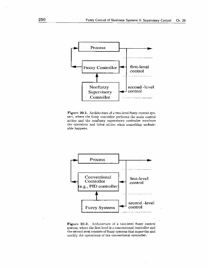
The fuzzy controllers considered in Chapters 17-19 are single-loop (or single-level) controllers; that is, the whole control system consists of the process and the fuzzy controller connected in a single loop. For complex practical systems, the single-loop control systems may not effectively achieve the control objectives, and a multi-level control structure turns out to be very helpful. Usually, the lower-level controllers perform fast direct control and the higher-level controllers perform low-speed su- pervision. In this chapter, we consider two-level control structures where one of the levels is constructed from fuzzy systems. We have two possibilities: (i) the first-level controller is a fuzzy controller and the second level is a nonfuzzy supervisory con- troller (see Fig. 20.1), and (ii) the first level consists of a conventional controller (for example, a PID controller) and the second level comprises fuzzy systems performing supervisory operations (see Fig. 20.2).
The main advantage of two-level control is that different controllers can be de- signed to target different objectives, so that each controller is simpler and perfor- mance is improved. Specifically, for the two-level control system in Fig. 20.1, we can design the fuzzy controller without considering stability and use the supervi- sory controller to deal with stability related problems. In this way, we have much freedom in choosing the fuzzy controller parameters and consequently, the design of the fuzzy controller is simplified and performance is improved. We will show the details of this approach in the next section. For the two-level control system in Fig. 20.2, we will consider the special case where the first level is a PID controller and the second-level fuzzy system adjusts the PID parameters according to certain heuristic rules; the details will be given in Section 20.3.
250 Fuzzy Control of Nonlinear Systems 1 1 : Supervisory Control Ch. 20
Process +
Fuzzy Controller first-level control
Nonfuzzy second -level Supervisory control Controller
Figure 20.1. Architecture of a two-level fuzzy control sys- tem, where the fuzzy controller performs the main control action and the nonfuzzy supervisory controller monitors the operation and takes action when something undesir- able happens.
Process
Fuzzy Systems n
+
+ first-level control
second -level control
I
Conventional Controller
(e.g., PID controller:
Figure 20.2. Architecture of a two-level fuzzy control system, where the first level is a conventional controller and the second level consists of fuzzy systems that supervise and modify the operations of the conventional controller.
+

Sec. 20.2. Stable Fuzzy Control Using Nonfuzzy Supervisor 251
20.2 Stable Fuzzy Control Using Nonfuzzy Supervisor
20.2.1 Design of the Supervisory Controller
Conceptually, there are at least two different approaches to guarantee the stabil- ity of a fuzzy control system. The first approach is to specify the structure and parameters of the fuzzy controller such that the closed-loop system with the fuzzy controller is stable (for example, the fuzzy controllers in Chapters 17 and 19). In the second approach, the fuzzy controller is designed first without any stability con- sideration, then another controller is appended to the fuzzy controller to take care of the stability requirement. Because there is much flexibility in designing the fuzzy controller in the second approach, the resulting fuzzy control system is expected to show better performance.
The key in the second approach is to design the appended second-level nonfuzzy controller to guarantee stability. Because we want the fuzzy controller to perform the main control action, the second-level controller would be better a safeguard rather than a main controller. Therefore, we choose the second-level controller to operate in the following supervisory fashion: if the fuzzy controller works well, the second-level controller is idle; if the pure fuzzy control system tends to be unstable, the second-level controller starts working to guarantee stability. Thus, we call the second-level controller a supervisory controller.
Consider the nonlinear system governed by the differential equation
dn) = f (z, 2 , ..., ~ ( ~ - l ) ) + g(z, x, ..., ~ ( ~ - l ) ) u (20.1)
where $1: E R is the output of the system, u E R is the control, x = (z, x, ..., x ( ~ - ' ) ) ~ is the state vector that is assumed to be measurable or computable, and f and g are un:known nonlinear functions. We assume that g > 0. From nonlinear control theory (Isidori [1989]) we know that this system is in normal form and many general nonlinear systems can be transformed into this form. The main restriction is that the control u must appear linearly in the equation.
Nolu suppose that we have already designed a fuzzy controller
for the system. This can be done, for example, by the trial-and-error approach in Cha,pter 16. Our task is to guarantee the stability of the closed-loop system and, at, the same time, without changing the existing design of the fuzzy controller UJ,,,(:K). More specifically, we are required to design a controller whose main control action is the fuzzy control uf,,,(x) and that the closed-loop system with this controller is globally stable in the sense that the state x is uniformly bounded, that is, Ix(t)l < Mx,Vt > 0, where Mx is a constant given by the designer.
For this task, we append the fuzzy controller uf,,,(x) with a supervisory con- troller us(x), which is nonzero only when the state x hits the boundary of the

252 Fuzzy Control of Nonlinear Systems II: Supervisory Control Ch. 20
constraint set {x : 1x1 < M z ) ; that is, the control now is
u = uf tL,, (x) + I*% (x) (20.3)
where the indicator function I* = 1 if 1x1 2 M, and I* = 0 if 1x1 < M,. Therefore, the main control action is still the fuzzy controller ufu,,(x). Our task now is to design the us such that Ix(t)l < M, for all t > 0.
Let us first examize whether it is possible to design such a supervisory controller without any additional assumption. Substituting (20.3) into (20.1) we have that the closed-loop system satisfies
x'"' = f (x) + ~ ( x ) ~ ~ u z z ( x ) + S(X)I*US(X) (20.4)
Now suppose 1x1 = M, and thus I* = 1. Because we assume that f(x) and g(x) are totally unknown and can be arbitrary nonlinear functions, for any us(x) we can always find f (x) and g(x) such that the right-hand side of (20.4) is positive, and therefore we will have 1x1 > M,. Thus, we must make additional assumptions for f(x) and g(x) in order for such us design to be possible. We need the following assumption.
Assumption 20.1: We can determine functions fU(x) and g ~ ( x ) such that If (x) 1 5 f (x) and 0 < g~ (x) < g(x), that is, we assume that we know the upper bound of If (x) I and the lower bound of g(x).
In practice, the bounds f U(x) and gL(x) usually are not difficult to find because we only require to know the loose bounds, that is, f U(x) can be very large and gL(x) can be very small. Also, we require to have state-dependent bounds, which is weaker than requiring fixed bounds.
Before we design the supervisory controller us, we need to write the closed-loop system equation into a vector form. First, define
where k = (k,, ..., k ~ ) ~ E Rn is such that all roots of the polynomial sn + klsn-I + ... + kn are in the left-half complex plane. Using this u*, we can rewrite (20.4) as
Define

Sec. 20.2. Stable Fuzzy Control Using Nonfuzzy Supervisor 253
then (20.6) can be written into the vector form
We now design the supervisory controller us to guarantee 1x1 5 Mx. Define the Lyapunov function candidate
1 V = - x T p x
2 (20.10)
where P is a symmetric positive definite matrix satisfying the Lyapunov equation
where Q > 0 is specified by the designer. Because A is stable, such P always exists. Using (20.9) and (20.11) and considering the case 1x1 2 Mx, we have
Our goal now is to design us such that v 5 0 , that is, the right-hand side of (20.12) is non-positive. Observing (20.12) and (20.5), we choose the us as follows:
Substituting (20.13) into (20.12) we have v 5 0. Therefore, the supervisory con- troller us of (20.13) guarantees that 1x1 is decreasing if 1x1 > Mx. Consequently, if we choose the initial Ix(O)I 5 M,, we will have Ix(t)l 5 Mx for all t > 0. Because g > 0 and x and P are available, s ign(xTPb) in (20.13) can be computed. Also, all other terms in (20.13) are available, thus the us of (20.13) can be implemented on-line.
Because the I* in (20.3) is a step function, the supervisory controller begins operation as soon as x hits the boundary 1x1 = Mx and is idle as soon as the x is back to the interior of the constraint set 1x1 5 Mz7 hence the system may oscillate across the boundary 1x1 = Mz. One way to overcome this "chattering" problem is to let I* continuousZg change from 0 to 1. Specifically, we may choose the I* as follows:
a 5 1x1 < Mx (20.14) 1 1x1 2 Mx

254 Fuzzy Control of Nonlinear Systems II: Supervisory Control Ch. 20
where a E (0, Mx) is a parameter specified by the designer. With this I* in (20.3), the supervisory controller us operates continuously from zero to full strength as x changes from a to Mx. Obviously, this I* can also guarantee that 1x1 5 Mx (Exercise 20.1).
20.2.2 Application to Inverted Pendulum Balancing
In this subsection, we apply a fuzzy controller together with the supervisory con- troller to the inverted pendulum balancing problem. The control objective is to balance the inverted pendulum and, at the same time, to guarantee that the state is bounded. The inverted pendulum system is illustrated in Fig. 1.9 and its dynamic equations are
where g = 9.8m/s2 is the acceleration due to gravity, mc is the mass of cart, m is the mass of pole, 1 is the half length of pole, and u is the applied force (control). We chose mc = lkg, m = O.lkg, and I = 0.5m in the following simulations. Clearly, (20.15)-(20.16) is in the form of (20.1), thus our approach applies to this system.
Assume that the fuzzy controller uf,,, is constructed from the following four fuzzy IF-THEN rules:
IF $1 i s positive and xz is positive, T H E N u i s negative big(20.17)
IF xl is positive and xz is negative, T H E N u i s zero (20.18)
IF xl i s negative and 2 2 i s positive, T H E N u i s zero (20.19)
IF x1 i s negative and 2 2 i s negative, T H E N u i s positive bid20.20)
where the fuzzy sets "positive," "negative," "negative big," "zero," and "positive big" are characterized by the membership functions
1 pnegative ($1 = --- 1 + e30x
(20.22)
Pnegative big (u) = e-(U+5)2 (20.23)
~zevo(u) = ePU2 (20.24)
~ l p o s i t i v e big (u) = e-(U-5)2 (20.25)
respectively. Using the center average defuzzifier and the product inference engine, we obtain the fuzzy controller uf,,, as follows:

Sec. 20.2. Stable Fuzzy Control Using Nonfuzzy Supervisor 255
To design the supervisory controller, we first need to determine the bounds f and g ~ . For this system, we have
If we require that lxl 1 5 7r/9 (we will specify the design parameters such that this requirement is satisfied), then
Our control objective is to balance the inverted pendulum from arbitrary initial angles xl E [ - ~ 1 9 , 7r/9] and at the same time to guarantee 1 I(x1, x2)I 12 5 7r/9 = Mx.
The design parameters are specified as follows: a = ~ 1 1 8 , kl = 2, k2 = 1 (so that s2 + kls + k2 is stable) and Q = diag(l0,lO). Then, we solve the Lyapunov equation (20.11) and obtain
We simulated three cases: (i) without the supervisory controller, that is, only use the fuzzy controller (20.26), (ii) use the supervisory controller together with the fuzzy controller, and (iii) same as (ii) except that a white Gaussian noise with variance 3 was added to the control u, which represents wind-gusts distur- bance. For each case, we simulated the closed-loop system for five initial conditions: (XI (O), x2 (0)) = (4O, O), (so, O), (12O, O), (16O, O), (20°, 0). The simulation results for cases (i), (ii) and (iii) are shown in Figs. 20.3, 20.4, and 20.5, respectively, where we show the angle xl(t) as a function of t for the five initial conditions. We see from these results that: (a) the pure fuzzy controller could balance the inverted pendulum for smaller initial angles 4O, 8" and 12O, but the system became unstable for larger initial angles 16' and 20°, (b) by appending the supervisory controller to the fuzzy controller, we successfully balanced the inverted pendulum for all the five initial angles and guaranteed that the angle is within [-20°, 20°], and (c) the fuzzy controller was robust to random disturbance.
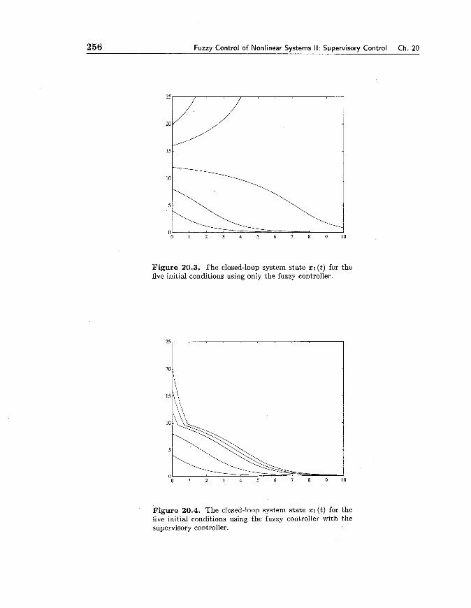
256 Fuzzy Control of Nonlinear Svstems II: Su~ervisorv Control Ch. 20
Figure 20.3, The closed-loop system state xl(t) for the five initial conditions using only the fuzzy controller.
Figure 20.4. The closed-loop system state xl(t) for the five initial conditions using the fuzzy controller with the supervisory controller.
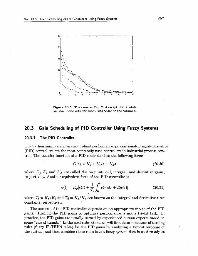
Sec. 20.3. Gain Scheduling of PID Controller Using Fuzzy Systems 257
Figure 20.5. The same as Fig. 20.4 except that a white Gaussian noise with variance 3 was added to the control u.
20.3 Gain Scheduling of PID Controller Using Fuzzy Systems
20.3.1 The PID Controller
Due to their simple structure and robust performance, proportional-integral-derivative (PID) controllers are the most commonly used controllers in industrial process con- trol. The transfer function of a PID controller has the following form:
where Kp, Ki and Kd are called the propositional, integral, and derivative gains, respectively. Another equivalent form of the PID controller is
where Ti = Kp/Ki and Td = Kd/Kp are known as the integral and derivative time constants, respectively.
The success of the PID controller depends on an appropriate choice of the PID gains. Turning the PID gains to optimize performance is not a trivial task. In practice, the PID gains are usually turned by experienced human experts based on some "rule of thumb." In the next subsection, we will first determine a set of turning rules (fuzzy IF-THEN rules) for the PID gains by analyzing a typical response of the system, and then combine these rules into a fuzzy system that is used to adjust
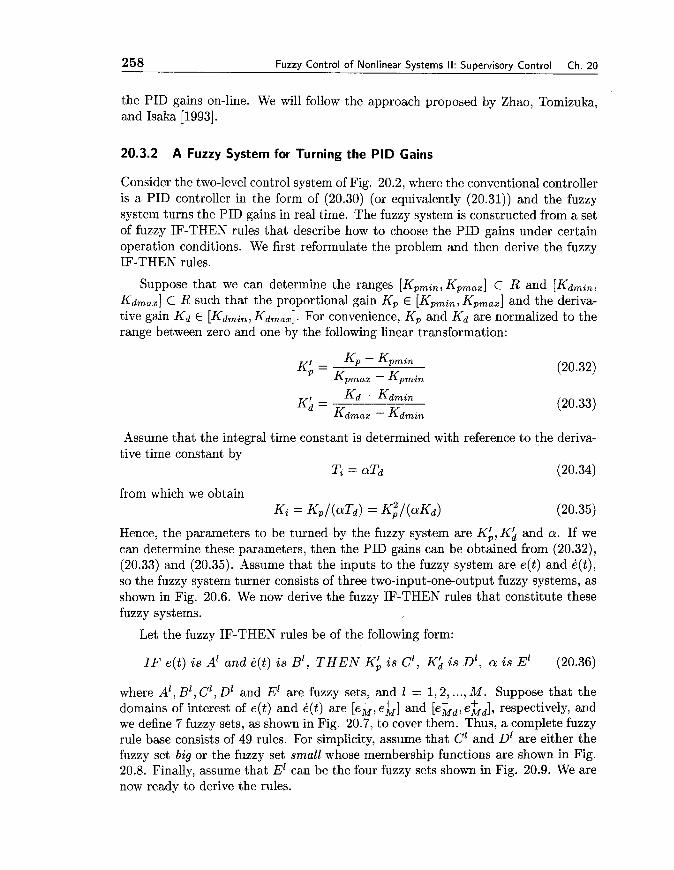
258 Fuzzy Control of Nonlinear Systems II: Supervisory Control Ch. 20
the PID gains on-line. We will follow the approach proposed by Zhao, Tomizuka, and Isaka [1993].
20.3.2 A Fuzzy System for Turning the PID Gains
Consider the two-level control system of Fig. 20.2, where the conventional controller is a PID controller in the form of (20.30) (or equivalently (20.31)) and the fuzzy system turns the PID gains in real time. The fuzzy system is constructed from a set of fuzzy IF-THEN rules that describe how to choose the PID gains under certain operation conditions. We first reformulate the problem and then derive the fuzzy IF-THEN rules.
Suppose that we can determine the ranges [Kpmin,Kpmax] C R and [Kdmin, Kdmax] C R such that the proportional gain Kp E [Kpmin, Kpmax] and the deriva- tive gain Kd E [Kdmin, Kdmax]. For convenience, Kp and Kd are normalized to the range between zero and one by the following linear transformation:
K' = Kp - Kpmin (20.32) Kpmax - Kpmin
KA = Kd - Kdmin Kdmax - Kdmin
Assume that the integral time constant is determined with reference to the deriva- tive time constant by
Ti = aTd (20.34)
from which we obtain Ki = Kp/(aTd) = K ; / ( ~ K ~ )
Hence, the parameters to be turned by the fuzzy system are KA, KA and a . If we can determine these parameters, then the PID gains can be obtained from (20.32), (20.33) and (20.35). Assume that the ir~puts to the fuzzy system are e(t) and B(t), so the fuzzy system turner consists of three two-input-one-output fuzzy systems, as shown in Fig. 20.6. We now derive the fuzzy IF-THEN rules that constitute these fuzzy systems.
Let the fuzzy IF-THEN rules be of the following form:
IF e(t) is A' and 6 ( t ) is B', T H E N Kh is c', K i is D1, a is E' (20.36)
where A', B1, C1, D1 and E k e fuzzy sets, and 1 = 1,2, ..., M. Suppose that the domains of interest of e(t) and k(t) are [e;, e&] and [eGd, ehd], respectively, and we define 7 fuzzy sets, as shown in Fig. 20.7, to cover them. Thus, a complete fuzzy rule base consists of 49 rules. For simplicity, assume that C1 and D1 are either the fuzzy set big or the fuzzy set small whose membership functions are shown in Fig. 20.8. Finally, assume that El can be the four fuzzy sets shown in Fig. 20.9. We are now ready to derive the rules.
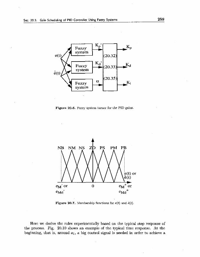
Figure 20.6. Fuzzy system turner for the PID gains.
Figure 20.7. Membership functions for e( t ) and d ( t ) .
Here we derive the rules experimentally based on the typical step response of the process. Fig. 20.10 shows an example of the typical time response. At the beginning, that is, around a l , a big control signal is needed in order to achieve a

260 Fuzzv Control of Nonlinear Svstems II: Su~ervisorv Control Ch. 20
Figure 20.8. Membership functions for KL and KA.
t S M S M B
Figure 20.9. Membership functions for a.
fast rise time. To produce a big control signal, we need a large proportional gain Kb, a small derivative gain Ki, and a large integral gain. From (20.35) we see that for fixed K, and Kd, the integral gain is inversely proportional to a, therefore a

Sec. 20.3. Gain Scheduling of PID Controller Using Fuzzy Systems 261
larger integral gain means a smaller a. Consequently, the rule around a1 reads
IF e(t) i s P B and B(t) i s 20, THEN KL is Big, K i is Small, a i s S (20.37)
where the membership functions for the fuzzy sets PB, 20, Big, Small, and S are shown in Figs. 20.7-20.9.
Figure 20.10. The typical step response of process.
Around point b l in Fig. 20.10, we expect a small control signal to avoid a large overshoot. So we need a small proportional gain, a large derivative gain, and a small integral gain. Thus, the following rule is taken:
IF e(t) is ZO and d(t) i s NB, THEN KL is Small, Ki is Big, a is B (20.38)
The control actions around points CI and dl are similar to those around points a1 and bl, respectively. Using this kind of idea, we can determine three sets of rules for Kk, K i and a, and each set consists of 49 rules. These three sets of rules are shown in Figs. 20.11-20.13, respectively.
We combine the 49 rules in each set using product inference engine, singleton fuzzifier, and center average defuzzifier; that is, the parameters Kk, K i and a are turned on-line according to
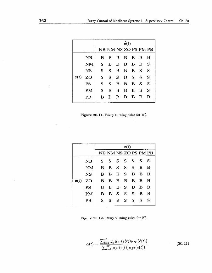
262 Fuzzy Control of Nonlinear Systems I I : Supervisory Control Ch. 20
Figure 20.11. Fuzzy turning rules for KL.
i(t> NB N M NS ZO PS PM PB
B B B B B B B
S B B B B B S
S S B B B S S
S S S B S S S
S S B B B S S
S B B B B B S
B B B B B B B
e(t)
Figure 20.12. Fuzzy turning rules for Ki .
NB
N M
NS
ZO
PS
PM
PB
i(t> NB N M NS ZO PS PM PB
S S S S S S S
B B S S S B B
B B B S B B B
B B B B B B B
B B B S B B B
B B S S S B B
S S S S S S S
e(t)
NB
N M
NS
ZO
PS
PM
PB

Sec. 20.4. Summary and Further Readings 263
Figure 20.13. Fuzzy turning rules for a.
where A1 and B' are shown in Fig. 20.7, and I;, and ji: are the centers of the corresponding fuzzy sets in Figs. 20.8 and 20.9 (according to the rules in Figs. 20.11-20.13).
Simulation results and comparison with classici~l methods can be found in Zhao, Tomizuka, and Isaka [1993].
20.4 Summary and Further Readings
In this chapter we have demonstrated the following:
The structure and working principles of two-level fuzzy control.
How to design the nonfuzzy supervisory controller to guarantee the global stability of the fuzzy control system.
How to derive fuzzy IF-THEN rules for turning the PID gains based on heuris- tic analysis of the typical step response.
Multi-level control has been studied in the field of intelligent robotics, see Vala- vanis and Saridis [I9921 and Tzafestas [1991]. The supervisory control idea in this chapter was proposed in Wang [1994b]. Using fuzzy systems to turn the PID pa- rameters was studied by a number of researchers and the approach in this chapter was due to Zhao, Tomizuka, and Isaka [1993].

264 Fuzzy Control of Nonlinear Systems II: Supervisory Control Ch. 20
20.5 Exercises
Exercise 20.1. Show that if we use the continuous indicator function I* of (20.14) in the controller (20.3) with the us given by (20.13), we can still guarantee that Jx(t) 1 < Mx for all t 2 0 if Ix(0) I < Mz. Furthermore, show that in this case there exists M i < Mz such that Ix(t)l < M; for all t 2 0 if Ix(O)I < M;.
Exercise 20.2. Discuss the similarities and differences between the supervisory controller in this chapter and the sliding controller in Chapter 19.
Exercise 20.3. Repeat the simulations in Subsection 20.2.2 with slightly dif- ferent fuzzy control rules and different initial conditions.
Exercise 20.4. In the PID controller (20.30), Kp, Ki/s, and Kds are called proportional, integral, and derivative modes, respectively. Use examples to show that:
(a) The proportional mode provides a rapid adjustment of the manipulated variable, does not provide zero steady-atate offset although it reduces the error, speeds up dynamic response, and can cause instability if tuned improperly.
(b) The integral mode achieves zero steady-state offset, adjusts the manipulated variable in a slower manner than the proportional mode, and can cause instability if tuned improperly.
(c) The derivative mode does not influence the final steady-state value of error, provides rapid correction based on the rate of change of the controlled variable, and can cause undesirable high-frequency variation in the manipulated variable.
Exercise 20.5. Consider the two-level fuzzy control system in Fig. 20.2, where the process is given by
27 G(s) =
(S + 1)(s + 3)3
the conventional controller is the PID controller, and the fuzzy systems are given by (20.39)-(20.41). Simulate this system and plot the process output. You may choose - + - any reasonable values for Kpmi,, Kp,ax, Kdmin, Kdmaz, e ~ , eM, eMd and eLd.

Chapter 21
Fuzzy Control of Fuzzy System Model
In Chapters 17-20, we studied the fuzzy control systems where the processes under control are represented by ordinary linear or nonlinear dynamic system models. In many practical problems, human experts may provide linguistic descriptions (in terms of fuzzy IF-THEN rules) about the process that can be combined into a model of the process; this model is called a fuzzy system model. Therefore, it is interesting to study the fuzzy control system in which the process is modeled by fuzzy systems and the feedback controller is a fuzzy controller; this is the topic of this chapter.
We will first introduce the Takagi-Sugeno-Kang (TSK) fuzzy system and derive the detailed formula of the closed-loop system in which the process and the controller are represented by the TSK fuzzy system. Then, we will analyze the stability of the closed-loop system. Finally, a design procedure for stable fuzzy controllers will be introduced.
21.1 The Takagi-Sugeno-Kang Fuzzy System
The Takagi-Sugeno-Kang (TSK) fuzzy system was proposed as an alternative to the fuzzy systems we have been using in most parts of this book. The TSK fuzzy system is constructed from the following rules:
IF 21 is C; and . . . and xn is c;, THEN y1 = cb + cixl + . . . + cix, (21.1)
where Cl are fuzzy sets, c: are constants, and 1 = 1,2, ..., M. That is, the IF parts of the rules are the same as in the ordinary fuzzy IF-THEN rules, but the THEN parts are linear combinations of the input variables. Given an input x = (XI, ..., x , ) ~ E U C Rn, the output f (x) E V C R of the TSK fuzzy system is computed as the weighted average of the yz's in (21.1), that is,

266 Fuzzy Control of Fuzzy System Models Ch. 21
where the weights wz are computed as
We see that the TSK fuzzy system is still a mapping from U c Rn to V c R. The physical meaning of the rule (21.1) is that when x is constrained to the fuzzy range characterized by the IF part of the rule, the output is a linear function of the input variables. Therefore, the TSK fuzzy system can be viewed as a somewhat piece-wise linear function, where the change from one piece to the other is smooth rather than abrupt. If c: = 0 for i = 1,2, ..., n and cb equals the center gE of the fuzzy set B' in the ordinary fuzzy IF-THEN rule (7.1), then the TSK fuzzy system is identical to the fuzzy system with product inference engine, singleton fuzzifier, and center average defuzzifier (comparing (21.2)-(21.3) with (9.1)).
If the output of a TSK fuzzy system appears as one of its inputs, we obtain the so-called dynamic TSK fuzzy system. Specifically, a dynamic TSK fuzzy system is constructed from the following rules:
IF x(k) i s A: and . .. and x(k - n + 1) i s AP, and u(k) is BP
T H E N xP(k + 1) = ayx(k) + . . + aP,x(k - n + 1) + bPu(k) (21.4)
where A: and BP are fuzzy sets, a: and b p are constants, p = 1,2, ... , N , ~ ( k ) is the input to the system, and x(k) = (x(k), x(k - I) , ..., x(k - n + l ) )T E Rn is the state vector of the system. The output of the dynamic TSK fuzzy system is computed as
where xp(k + 1) is given in (21.4) and
We will use this dynamic TSK fuzzy system to model the process under control.
21.2 Closed-Loop Dynamics of Fuzzy Model with Fuzzy Con- troller
Consider the feedback control system in Fig. 21.1, where the process under control is modeled by the dynamic TSK fuzzy model (21.5), and the controller is the TSK fuzzy system (21.2) with cb = 0 and xi = x( t - i+ 1) for i = 1,2, ..., n. The following theorem gives the closed-loop dynamics of the control system in Fig. 21.1.
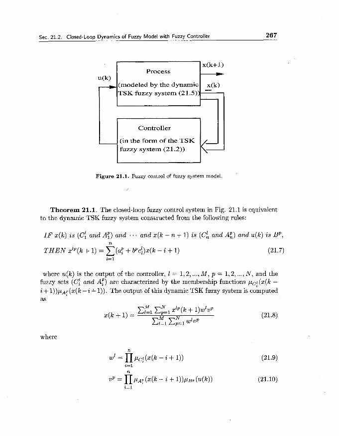
Sec. 21.2. Closed-Loop Dynamics of Fuzzy Model with Fuzzy Controller 267
Figure 21.1. Fuzzy control of fuzzy system model.
,
u(k) -
Theorem 21.1. The closed-loop fuzzy control system in Fig. 21.1 is equivalent to the dynamic TSK fuzzy system constructed from the following rules:
x(k+ 1) Process
(modeled by the dynamic x(k) - TSK fuzzy system (21.5))
IF x ( k ) is (c! and A:) and . . . and x(k - n + 1) i s (c: and A:) and u ( k ) is B P , n
T H E N xzP(k + 1) = x ( a f + bpci)x(k - i + 1) (21.7) i= 1
Controller
(in the form of the TSK fuzzy system (21.2))
where u ( k ) is the output of the controller, I = 1,2, ..., M , p = 1,2, ..., N , and the fuzzy sets (C: and A:) are characterized by the membership functions pc! ( x ( k - i + l ) ) p A p ( x ( k - i + 1)). The output of this dynamic TSK fuzzy system is computed as
where

268 Fuzzy Control of Fuzzy System Models Ch. 21
Proof: From Fig. 21.1 we see that the u ( k ) in (21.4) equals the f ( x ) of (21.2). Hence, xp(k + 1) in (21.4) becomes
Substituting (21.11) into (21.5), we obtain the output of the closed-loop system
which is (21.8).
Example 21.1. Suppose that the process in Fig. 21.1 is modeled by a second- order dynamic TSK fuzzy system that is constructed from the following two rules:
L' : I F x ( k ) is A: and x (k - 1) is A; and u ( k ) is B ~ ,
T H E N x l ( k + 1) = 1.5x(k) + 2.lx(k - 1) - u ( k ) (21.13)
L' : I F x ( k ) is AT and x ( k - 1) is A; and u ( k ) is B2,
T H E N x2(k + 1) = 0.3x(k) - 3.4x(k - 1) + 0.5u(k) (21.14)
and that the controller in Fig. 21.1 is a TSK fuzzy system constructed from the following two rules:
R1 : I F x ( k ) is C; and x (k - 1) is c:, T H E N u l ( k ) = k:x(k) + k i x ( k - 1) (21.15)
R~ : I F x ( k ) is C; and x (k - 1) is Cg,
T H E N u2 (k ) = k;x(k) + kgx(k - 1) (21.16)
Then from Theorem 21.1 we have that the closed-loop system is a dynamic TSK fuzzy system constructed from the following four rules:
S1' : I F x ( k ) is (A: and C!) and x (k - 1) is (A: and c;) and u ( k ) is B 1 ,
T H E N x l l ( k + 1) = (1.5 - k i ) x ( k ) + (2.1 - k i ) x ( k - 1) (21.17)
S12 : I F x ( k ) is (A: and c:) and x ( k - 1) is (A; and c;) and u ( k ) is B', T H E N x12(k + 1) = (1.5 - k:)x(k) i- (2.1 - e ) x ( k - 1) (21.18)

Sec. 21.3. Stability Analysis of the Dynamic TSK Fuzzy System 269
s2' : IF x(k) is (A! and Ci) and x(k - 1) is (A: and C;) and u(k) is B ~ ,
THEN x2l(k + 1) = (0.3 + 0.5k:)x(k) + (-3.4 + 0.5ki)x(k - 1) (21.19)
s~~ : IF x(k) is (A; and c;) and x(k - 1) is (A; and c;) and u(k) is B ~ , THEN x22(k + 1) = (0.3 + 0.5k;)x(k) + (-3.4 + 0.5k:)x(k - 1) (21.20)
The dynamic equation can be obtained according to (21.8)-(21.10).
Since the closed-loop fuzzy control system in Fig. 21.1 is equivalent to a dynamic TSK fuzzy system, it is therefore important to study the stability of the dynamic TSK fuzzy system; this is the topic of the next section.
21.3 Stability Analysis of the Dynamic T S K Fuzzy System
Consider the dynamic TSK fuzzy system (21.5) with bp in (21.4) equal zero. We assume bP = 0 because comparing (21.4) with (21.7) we see that there is no bPu(k) term in (21.7). Define the state vector x(k) = (x(k), z(k - I) , ..., x(k - n i- I ) ) ~ and
Then the dynamic TSK fuzzy system (21.5) can be rewritten as \
where UP is defined in (21.6). Since the right-hand side of (21.22) equals zero when x(k) = 0, the origin in Rn is an equilibrium point of the dynamic system (21.22). We now use the following well-known Lyapunov stability theorem to study the stability of the dynamic system (21.22)
Lyapunov Stability Theorem: Consider the discrete-time system described by
~ ( k f 1) = f [x(k)] (21.23)
where x(k) E Rn and f (0) = 0. Suppose that there exists a scalar function V[x(k)] such that: (a) V(0) = 0, (b) V[x(k)] > 0 for x(k) # 0, (c) V[x(k)] -+ m as (Ix(k)ll -+ m , and (d) AV[x(k)] = V[x(k + l ) ] - V[x(k)] < 0 for x(k) # 0, then the equilibrium point 0 of the system (21.23) is globally asymptotically stable.
In order to apply this theorem to the system (21.22), we need the following lemma.

270 Fuzzy Control of Fuzzy System Models Ch. 21
Matr ix Inequality Lemma: If P is a positive definite matrix such that
where A, B, P E Rnxn, then
Proof of this lemma is left as an exercise. Using the Lyapunov Stability Theorem and the Matrix Inequality Lemma, we obtain the following theorem on the stability of the dynamic TSK fuzzy system (21.22).
Theorem 21.2. The equilibrium point 0 of the dynamic TSK fuzzy system (21.22) is globally asymptotically stable if there exists a common positive definite matrix P such that
A;PA,-P < 0 (21.26)
for all p = 1,2, ..., N.
Proof: Consider the Lyapunov function candidate
where P is a positive definite matrix. This V[x(k)] satisfies conditions (a)-(c) in the Lyapunov Stability Theorem; we now show that it also satisfies condition (d). Using (21.22), we have
Rearrange the summations, (21.28) becomes
From (21.26), the Matrix Inequality Lemma, and the fact that U P > 0, we con- clude that AV[x(k)] < 0. Hence, this theorem follows from the Lyapunov Stability Theorem. I7

Sec. 21.3. Stability Analysis of the Dynamic T S K Fuzzy System 271
Figure 21.2. Membership functions for the fuzzy sets in the rules (21.30)-(21.31).
Theorem 21.2 gives a sufficient condition for ensuring the stability of the dynamic TSK fuzzy system (21.22). We may intuitively guess that the nonlinear system (21.22) is stable if all locally approximate linear systems A, (p = 1,2, ..., N) are stable (the linear system x(k + 1) = A,x(k) is stable if all the eigenvalues of A, are within the unit circle). However, this is not true in general, as we notice that even if all the Abs are stable, there may not exist a common positive definite matrix P such that (21.26) is true. The following example shows that two locally stable linear systems result in an unstable nonlinear system.
Example 21.2. Consider a dynamic TSK fuzzy system constructed from the following two rules:
IF x(k - 1) i s F l , T H E N xl(k + 1) = x(k) - 0.5x(k - 1) (21.30) IF x(k - 1) i s F2, T H E N x2(k + 1) = -x(k) - 0.5x(k - 1) (21.31)
where the membership functions of the fuzzy sets Fl and F2 are shown in Fig. 21.2. For this system, we have
The eigenvalues of A1 and A2 are and y, respectively, which are all within the unit circle, so the two locally approximate linear systems x(k+ 1) = Alx(k) and x(k+ 1) = Asx(k) are stable. However, the dynamic TSK fuzzy system constructed
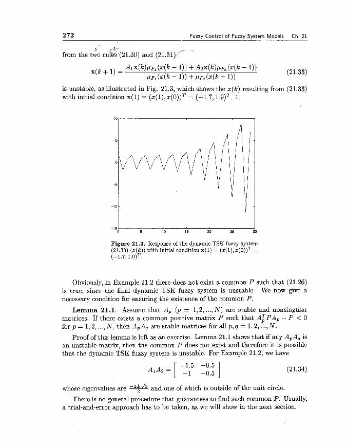
272 Fuzzy Control of Fuzzy System Models Ch. 21
I
from the tie ru3gr(21.30) and ( 2 1 . 3 1 ) c
is unstable, as illustrated in Fig. 21.3, which shows the ~ ( k ) resulting from (21.33) with initial condition x(1) = (%(I), ~ ( 0 ) ) ~ = (-1.7,1.9)~.
Figure 21.3. Res~onse of the dynamic TSK fuzzy system - "
(21.33) ( z ( k ) ) with initial condition x(1) = ( z ( l ) , ~ ( 0 ) ) ~ = (-1.7,1.9)~.
Obviously, in Example 21.2 there does not exist a common P such that (21.26) is true, since the final dynamic TSK fuzzy system is unstable. We now give a necessary condition for ensuring the existence of the common P.
Lemma 21.1. Assume that A, (p = 1,2, .. ., N) are stable and nonsingular matrices. If there exists a common positive matrix P such that ATPA, - P < 0 for p = 1,2, ..., N, then ApAq are stable matrices for all p, q = 1,2, ..., N.
Proof of this lemma is left as an exercise. Lemma 21.1 shows that if any ApAq is an unstable matrix, then the common P does not exist and therefore it is possible that the dynamic TSK fuzzy system is unstable. For Example 21.2, we have
whose eigenvalues are and one of which is outside of the unit circle.
There is no general procedure that guarantees to find such common P. Usually, a trial-and-error approach has to be taken, as we will show in the next section.

Sec. 21.4. Design of Stable Fuzzy Controllers for the Fuzzy Model 273
21.4 Design of Stable Fuzzy Controllers for the Fuzzy Model
In Theorem 21.2, a sufficient condition was given to ensure the stability of the dynamic TSK fuzzy system. In Theorem 21.1, it was proven that the closed-loop fuzzy control system in Fig.21.1 can be represented as a dynamic TSK fuzzy system. Therefore, we can use Theorem 21.2 to design stable fuzzy controllers for the fuzzy system model; this is the topic of this section.
Since there is no systematic way to find the common P in Theorem 21.2, our design procedure, which is given below, has to be trial and error in nature.
Design of Stable Fuzzy Controller for Fuzzy System Model:
Step 1. Use Theorem 20.1 to represent the closed-loop fuzzy control system as a dynamic TSK fuzzy system. The parameters a: and bp and the membership functions p p for the process are known, and those for the controller (that is, c: and pc!) are to be designed. Usually, fix the p,; and design the cf according to ?heorem 21.2.
Step 2. Choose the parameters cf such that all the locally approximate linear systems are stable, where, according to (21.7), the locally approximate linear systems are x(k + 1) = Alpx(k) with
where 1 = l ,2 , ..., M , and p = l ,2 , ..., N.
Step 3. Find positive definite matrices Plp such that
for I = 1,2, ..., M and p = 1,2, ..., N. If there exists Ppp* for some fixed I* E {1,2, ..., M ) and p* E {1,2, ..., N) such that
for all 1 = 1,2, ..., M and p = 1,2, ..., N, then select this PZ*,. as the common P; otherwise, go to Step 2 to redesign the parameters 4 until the common P = Pl.,. is found.
Since there is much freedom in choosing the parameters cf in Step 2, it is possible that we can find the common P after several iterations. Of course, we cannot guarantee that such common P can be found. We now test the design procedure through an example.

2 74 Fuzzv Control of Fuzzv Svstern Models Ch. 21
Example 21.3. Suppose that the process is modeled by a dynamic TSK fuzzy system with the following two rules:
I F x ( k ) is G I , T H E N x l ( k + 1) = 2.18x(k) - 0.59x(k - 1)
-0.603~(k) (21.38)
I F x ( k ) is G2, T H E N x2(k + 1) = 2.26x(k) - 0.36x(k - 1)
-1 .120~(k) (21.39)
and the controller is a TSK fuzzy system constructed from the two rules:
I F x ( k ) is G l , T H E N u l ( k ) = c:x(k) + cix(k - 1) (21.40)
I F x ( k ) is G 2 , T H E N u2 (k ) = cTx(k) + c;x(k - 1) (21.41)
where the membership functions for G I and G2 are shown in Fig. 21.4, and the controller parameters c i , c i , cf and ci are to be designed such that the closed-loop system is stable.
Figure 21.4. Membership functions for the fuzzy sets in Example 21.3.
Step 1. From Theorem 21.1 we obtain that the closed-loop system is a dynamic TSK fuzzy system constructed from the following four rules:
I F x ( k ) is (GI and G 2 ) , T H E N x l1(k + 1) = (2.18 - 0.603c:)x(k) +(-0.59 - 0.603c~)x(k - 1) (21.42)
I F s ( k ) is (GI and G z ) , THEN x12(k + 1) = (2.18 - 0.603c:)x(k) +(-0.59 - 0.603c;)x(k - 1) (21.43)

Sec. 21.5. Summary and Further Readings 275
IF x(k) is (GI and Gz), THEN x2l(k + 1) = (2.26 - 1.120c:)x(k)
+(-0.36 - 1.120ci)x(k - 1) (21.44)
IF x(k) is (GI and Gz), THEN x22(k + 1) = (2.26 - 1.120c:)x(k)
+(-0.36 - 1.120c;)x(k - 1) (21.45)
Step 2. The four matrices Alp for the four linear subsystems (21.42)-(21.45) are
After much trial and error, we found that if we choose
then all the four linear subsystems are stable.
Step 3. We found that a common P can be found for the parameters in (21.50). Therefore, our stable fuzzy controller is the TSK fuzzy system constructed from the two rules (21.40)-(21.41) with the parameters given by (21.50).
21.5 Summary and Further Readings
In this chapter we have demonstrated the following:
The static and dynamic TSK fuzzy systems.
The dynamic equation of the closed-loop system in which the process is mod- eled by a dynamic TSK fuzzy system and the controller is a static TSK fuzzy system.
Conditions that ensure the stability of the above closed-loop system.
How to design the fuzzy controller such that the closed-loop system above is stable.
Using the TSK fuzzy systems to model nonlinear systems was studied in Takagi and Sugeno [I9851 and Sugeno and Kang [1988]. The stability analysis in this chapter was due to Tanaka and Sugeno [I9921 where more examples can be found.

2 76 Fuzzv Control of Fuzzv Svstem Models Ch. 21
21.6 Exercises
Exercise 21.1. Prove the Matrix Inequality Lemma.
Exercise 21.2. If we change condition (d) in the Lyapunov Stability Theorem to AV[x(k)] = V[x(k + I)] - V[x(k)] < 0 for x(k) in a neighborhood of 0, then the conclusion becomes that the system is asymptotically stable. Prove that the system
is asymptotically stable.
Exercise 21.3. Prove Lemma 21.1.
Exercise 21.4. Consider the dynamic TSK fuzzy system (21.22) with N = 2. Suppose that Al and Az are stable and A1A2 = A2A1. Given Po > 0, determine the matrices PI and P 2 from
Prove that P2 is the common P in Theorem 21.2.
Exercise 21.5. Generalize the procedure of finding the common P in Exercise 21.4 to arbitrary N.
Exercise 21.6. Suppose that the process under control is modeled by a dynamic TSK fuzzy system constructed from the rules (21.38) and (21.39). Design a linear controller u(k) = Kx(k) (that is, determine the constant K ) such that the closed- loop system is stable.
Exercise 21.7. Repeat Exercise 21.6, with the fuzzy sets G1 and Gz replaced by the fuzzy sets Fl and F2 in Fig. 21.2, respectively.

Chapter 22
Qualitative Analysis of Fuzzy Control and Hierarchical Fuzzy
Systems
22.1 Phase Plane Analysis of Fuzzy Control Systems
Phase plane analysis is a graphical method for studying second-order systems. The basic idea is to generate motion trajectories of the system in the state space corre- sponding to various initial conditions, and then to examine the qualitative features of the trajectories. In this way, information concerning stability, robustness and other properties of the system can be obtained. The state space for second-order systems is called the phase plane.
The main advantage of phase plane analysis is its graphical nature, which allows us to visualize what goes on in a nonlinear system starting from different initial conditions, without having to solve the nonlinear equations analytically. The main disadvantage of the method is that it is restricted to second-order systems and is difficult to generalize to higher-order systems.
We now use the phase plane method to study second-order fuzzy control systems. Let x = (xl, be the state and consider the fuzzy control system
x = f (x) + bu u = +(x)
where f (x) is a nonlinear vector function (vector field) representing the plant dy- namic, b is a two-dimensional vector, u is a scalar control variable, and +(x) is a two-input-one-output fuzzy system. To study this closed-loop fuzzy control system, it is helpful to identify which rules are firing along a certain trajectory. Suppose that we define Nl and N2 fuzzy sets to cover the domains of XI and 22, respectively, and that the fuzzy rule base of @(x) consists of Nl x N2 rules. Let the l'th rule in

2 78 Qualitative Analysis of Fuzzy Control and Hierarchical Fuzzy Systems Ch. 22
the fuzzy rule base be
IF XI is A! and x2 is A;, T H E N y is B' (22.3)
Then we say that the point (xl, x2) in the phase plane belongs to rule I* if it holds that
PAP (XI ) * PA? ( ~ 2 ) 2 PA; (XI) * PA; ( ~ 2 ) (22.4) for all 1 # l*, where * represents t-norm.
Consider the fuzzy rule base in Fig.22.1, where Nl = N2 = 5 and the fuzzy rule base contains 25 rules. As shown in Fig.22.1, the state space of interest is partitioned into 25 regions, with each region belonging to a rule. For a given initial condition, the closed-loop system trajectory of (22.1)-(22.2) can be mapped onto the partitioned state space of Fig. 22.1. A trajectory corresponds to a sequence of rules that fire along the trajectory; this sequence of rules is called the linguistic trajectory, corresponding to the state trajectory. For the trajectory in Fig. 22.1, the corresponding linguistic trajectory is
Linguistic trajectory = (rulel6, rule21, rule22, rule23, rule24, rulel9, rulel4,
rule9, rule4, ruEe3, rule2, rule7, rulel2, rulel7,
rule18, rulel3) (22.5)
Figure 22.1. An example of linguistic trajectory.
By modifying the rules in the linguistic trajectory, we can change the corre- sponding state trajectory. For example, if we feel that the state trajectory in Fig.

Sec. 22.1. Phase Plane Analysis of Fuzzy Control Systems 2 79
22.1 converges too slowly in the early stage, we may modify, for example, rule 22 and rule 23 such that the convergence becomes faster. This can be done by noticing that the tangent vector of the state trajectory equals the summation of vector field f (x) and vector field b@(x), as shown in Fig. 22.2. If the point x in Fig. 22.2 belongs to rule 23, then by increasing the center value of the THEN-part fuzzy set of rule 23, we can increase the value of b+(x) at this point and therefore speed up convergence. The advantage of the phase plane analysis is that it helps us to identify the rules that influence the behavior of the trajectory, so that we only need to modify these rules to achieve the desired behavior.
Figure 22.2. The state trajectory moves along the direc- tion of the vector field f (x) + b@(x).
For the closed-loop fuzzy control system (22.1)-(22.2), we should pay special attention to the subspace @(x) = 0, which is a line in the phase plane. This line separates the phase plane into positive and negative control regions. It also is called the switching line because when the state trajectory goes across this line, the control changes from positive to negative and vice versa. When the state vector is far away from the switching line, the control vector b@(x) usually has greater influence on the closed-loop system than the plant component f (x). When the state vector gets closer to the switching line, b@(x) becomes smaller so that f (x) has more influence on the closed-loop system. The relationship between b@(x) and f (x) determines the behavior of the closed-loop system. Two situations are of most interests to us:
Stable closed-loop systems. This is often the case where the open-loop system x = f (x) is stable and the control u = @(x) tries to lead the system trajectory

280 Qualitative Analysis of Fuzzy Control and Hierarchical Fuzzy Systems Ch. 22
towards the switching line @(x) = 0. When the trajectory approaches the switching line, the plant component f (x) has a greater influence, which makes the trajectory converge to the equilibrium point. See Fig. 22.3 for an example.
Figure 22.3. An example of stable closed-loop system.
Limit cycles. This may be the case when the open-loop system x = f(x) is unstable and the control u = @(x) tries to stabilize the system. When the state is far away from the switch line @(x) = 0, the control cP(x) has a greater influence so that the state trajectory converges towards the switching line. When the state trajectory moves near the switching line, the unstable plant component f (x) has a greater influence, which makes the state trajectory diverge away from the equilibrium point. This interaction between the control and the plant components makes the state oscillate around the equilibrium point and a limit cycle is thus formed. Fig. 22.4 shows an example.
Although the phase plane analysis is qualitative, it is helpful to characterize the dynamic behavior of a fuzzy control system. It also can serve as the basis for adequate selection or modification of the rules.
22.2 Robustness Indices for Stability
We know that a linear control system is stable if the eigenvalues of the closed-loop system are in the open left-half complex plane. If the eigenvalues are close to the imaginary axis, then small changes of the parameters may move some eigenvalues
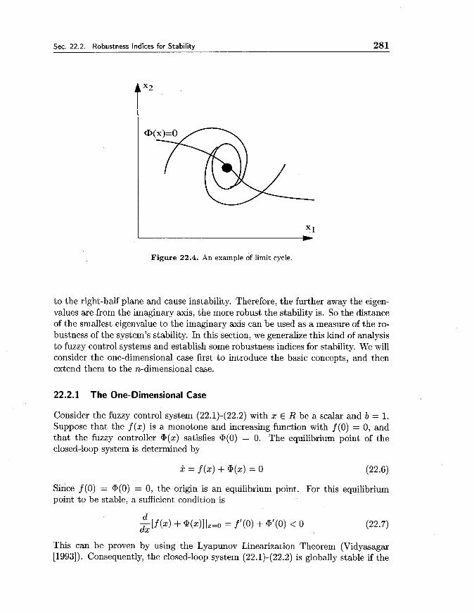
Sec. 22.2. Robustness Indices for Stability 281
Figure 22.4. An example of limit cycle.
to the right-half plane and cause instability. Therefore, the further away the eigen- values are from the imaginary axis, the more robust the stability is. So the distance of the smallest eigenvalue to the imaginary axis can be used as a measure of the ro- bustness of the system's stability. In this section, we generalize this kind of analysis to fuzzy control systems and establish some robustness indices for stability. We will consider the one-dimensional case first to introduce the basic concepts, and then extend them to the n-dimensional case.
22.2.1 The One-Dimensional Case
Consider the fuzzy control system (22.1)-(22.2) with x E R be a scalar and b = 1. Suppose that the f (x) is a monotone and increasing function with f (0) = 0, and that the fuzzy controller @(x) satisfies @(0) = 0. The equilibrium point of the closed-loop system is determined by
Since f (0) = cP(0) = 0, the origin is an equilibrium point. For this equilibrium point to be stable, a sufficient condition is
This can be proven by using the Lyapunov Linearization Theorem (Vidyasagar [1993]). Consequently, the closed-loop system (22.1)-(22.2) is globally stable if the

282 Qualitative Analysis of Fuzzy Control and Hierarchical Fuzzy Systems Ch. 22
following two conditions are satisfied:
Condition 1 : f l ( 0 ) + G1(0) < 0 (22.8) Condit ion 2 : l@(x)l < I f ( x ) I , V x # 0 (22.9)
Condition 1 ensures that the origin is a stable equilibrium point, while Condition 2 guarantees no intersection of curves @ ( x ) and - f ( x ) and therefore prevents the appearance of other equilibrium points.
If stability is lost, then either the equilibrium at the origin becomes unstable, or new equilibrium points are produced due to the intersection of @ ( x ) and - f ( x ) . Referring to (22.8) we see that the number
can be used to measure the robustness of stability of the equilibrium at the origin. The larger the value of 4, the more robust the stability of the origin. I1 of (22.10) is our first robustness index for stability of the fuzzy control system.
Similarly, a measure can be associated with Condition 2. This measure should correspond to the minimum distance between @ ( x ) and - f ( x ) , that is, minl@(x) + f ( $ ) I . However, since m i n l @ ( x ) + f (x)l equals zero when x = 0 , the min should be taken over the range that excludes a neighborhood of the origin. This gives our second robustness index for stability
I 2 = min I @ ( % ) + f (x ) l (22.11) xER-(-a,a)
where a is a positive constant. The larger the value of 12, the more robust the stability of the fuzzy control system.
22.2.2 T h e n-Dimensional Case
Let us start with n = 2 and then generalize to arbitrary n. Assume that f ( 0 ) = 0 and @ ( O ) = 0 , so the origin is an equilibrium point of the closed-loop system (22.1)- (22.2). From the Lyapunov Linearization Theorem (Vidyasagar [1993]) we know that the origin is stable if the two eigenvalues of the linearized system around the origin have negative real parts. Generally, there are two ways in which the system can become unstable:
A real eigenvalue crosses the imaginary axis and acquires a positive sign. This is called static bifurcation.
A pair of complex eigenvalues cross the imaginary axis and both of them take positive real parts. This is called Hopf bifurcation.
We now examine under what conditions these two bifurcations may occur.

Sec. 22.2. Robustness Indices for Stabilitv 283
Let
be the Jacobian matrix of f (x) + @(x) at the origin. Then, the eigenvalues of the linearized system at the origin are the solution of the characteristic equation
A static bifurcation is produced when a real eigenvalue crosses the imaginary axis, that is, when one of the roots of (22.13) is zero. This will happen, as we can see from (22.13), only when alla22 - al2a21 = 0. The larger the value of lallaz2 - al2aZ11, the further away the system is from static bifurcation. Therefore, we define
as a robustness index for stability for the second-order fuzzy control system. Simi- larly, a Hopf bifurcation may occur when the real parts of the two complex eigenval- ues equal zero. From (22.13) we see that this will happen only when all + a22 = 0. The larger the value of la11 +azz[, the more unlikely the Hopf bifurcation. Therefore, we define
I: = la11 +a221 = Itr(J)I (22.15)
as another robustness index. In summary, the larger the values of Il and I:, the more robust the stability of the fuzzy control system is.
Similar to the one-dimensional case, stability may be lost when the vector field of the fuzzy controller b*(x) compensates exactly the vector field of the plant f (x). Let b = (bl , bz) and f (x) = (fl (x), f2 (x)), then the compensation of the vector fields of the plant and the controller can occur only in the region of the state space where the plant component has the direction (bl, bz), that is, in the region defined by
Similar to the I2 of (22.11) for the one-dimensional case, we define the robustness index as
I 2 = min If(x) + b@(x)l xEC-B
(22.17)
where B = {x E R211x(2 5 a} is a ball around the origin.
For the general n > 2 cases, let
be the Jacobian matrix of the closed-loop system around the origin and

284 Qualitative Analvsis of Fuzzv Control and Hierarchical Fuzzv Svstems Ch. 22
be its characteristic polynomial. Similar to the n = 2 case, an = 0 may cause static bifurcation. Therefore, we define
as a robustness index. Similar to I; of (22.15), we can define a robustness index for Hopf bifurcation. Finally, the generalization of 1 2 (22.17) to the n > 2 case can be done by noticing that the subspace C of (22.16) now becomes
Example 22.1. Consider the fuzzy control system
The Jacobian matrix of this system at the origin is
If there is no control, that is, if @(xl, x2) = 0, then the robustness indices I; and I: are
I1 = 12.74, 1; = 2.22 (22.25)
With fuzzy controller @(XI, z2), these indices become
Therefore, if we design the fuzzy controller such that ~ / x , = x 2 = o < 0 and
~ / x l = x 2 = 0 < 0, then the closed-loop fuzzy control system will be more robust than the uncontrolled open-loop system.
22.3 Hierarchical Fuzzy Control
22.3.1 The Curse of Dimensionality
In Chapters 10 and 11 we saw that in order to design a fuzzy system with the required accuracy, the number of rules has to increase exponentially with the number of input variables to the fuzzy system. Specifically, suppose there are n input variables and m fuzzy sets are defined for each input variable, then the number of rules in the fuzzy system is mn. For large n, mn is a huge number. In practice,

Sec. 22.3. Hierarchical Fuzzv Control 285
it is not uncommon to have, say, five input variables. With n = 5 and m = 3 (usually, at least three fuzzy sets should be defined for each variable), mn = 243; if m = 5, which is more likely than m = 3, we have mn = 3120. It is impractical to implement a fuzzy system with thousands of rules. A serious problem facing fuzzy system applications is how to deal with this rule explosion problem.
In fact, it is a common phenomenon that the complexity of a problem increases exponentially with the number of variables involved; this is not unique to fuzzy systems. This phenomenon was identified by Bellman as "the curse of dimension- ality." Some approaches have been proposed to deal with this difficulty; using the hierarchical fuzzy system is one approach. We will see that the hierarchical fuzzy system has the nice property that the number of rules needed to the construct the fuzzy system increases only linearly with the number of variables.
22.3.2 Construction of the Hierarchical Fuzzy System
The idea of the hierarchical fuzzy system is to put the input variables into a col- lection of low-dimensional fuzzy systems, instead of a single high-dimensional fuzzy system as is the usual case. Each low-dimensional fuzzy system constitutes a level in the hierarchical fuzzy system. Suppose that there are n input variables X I , ..., x,, then the hierarchical fuzzy system is constructed as follows:
The first level is a fuzzy system with n l input variables X I , ..., x,, which is constructed from the rules
IF x1 i s A: and . . - and x,, i s A:,, T H E N yl i s ~4 (22.27)
where 2 5 nl < n, and 1 = 1,2, ..., MI.
The i'th level (i > 1) is a fuzzy system with ni + 1 (ni 2 1) input variables, which is constructed from the rules
I F XIV~+I is AL;+, and .. . and xiVi+ni i s Ahi+,, and yiPl i s c:-~, T H E N yi i s ~f (22.28)
where Ni = nj , and 1 = 1,2, ..., Mi.
L The construction continues until i = L such that C j = , n j = n, that is, until all the input variables are used in one of the levels.
We see that the first level converts n l variables X I , ..., x,, into one variable y1, which is then sent to the second level. In the second level, other na variables xnl+l, ..., x,*+,~ and the variable yl are combined into another variable yz, which is sent to the third level. This process continues until all the variables $1, ..., x, are used.

286 Qualitative Analysis of Fuzzy Control and Hierarchical Fuzzy Systems Ch. 22
A special case of the hierarchical fuzzy system is to choose n l = 2 and ni = 1 for i = 2,3, ... , L. In this case, all the fuzzy systems in the hierarchy have two inputs, and there are L = n - 1 levels. This special hierarchical fuzzy system is illustrated in Fig. 22.5.
fuzzy syste A fuzzy syste
fuzzy syste
4 fuzzy syste + A1 Yn-2
... ...
Figure 22.5. An example of hierarchical fuzzy system with nl = 2 and ni = 1 for i = 2,3, ..., n - 1. This hi- erarchical fuzzy system consists of n - 1 two-input fuzzy systems.
Next, we study the properties of the hierarchical fuzzy system.
22.3.3 Properties of the Hierarchical Fuzzy System
We now show that the number of rules in the hierarchical fuzzy system is a linear function of the number of input variables (Theorem 22.1) and that the rule number reaches its minimum in the special case of Fig. 22.5 (Theorem 22.2).
Theorem 22.1. Let n, ni and L be the same as in the design of the hierarchical fuzzy system. Suppose that m fuzzy sets are defined for each variable, including the input variables X I , ..., xn and the intermediate variables yl, ..., y ~ , and that the fuzzy system in the i'th level (i = 2, ..., L) is constructed from mnt+' rules (a complete fuzzy rule base) and for the first level the rule number is mnl. If n1 = ni + 1 = c (constant) for i = 2,3, ..., L, then the total number of rules in the whole hierarchical fuzzy system is
mC M = -(n- 1) (22.29)
c - 1

Sec. 22.4. Summary and Further Readings 287
Proof: Obviously, we have
Since n = c:', ni = c + ~ : , ( c - 1) = LC - L + 1, we have
Substituting (22.31) into (22.30), we obtain (22.29).
Since 5 is a constant, we see from (22.29) that the number of rules in the hierarchical fuzzy system increases linearly with the number of input variables. For the case of m = 3,c = 2 and n = 5, we have M = 3,4 = 36; if we use the conventional fuzzy system, the number of rules is mn = 35 = 243. The reduction of rules is even greater for larger m and n.
Finally, we show that the rule number M reaches its minimum when c = 2.
Theorem 22.2. Let the assumptions in Theorem 22.1 be true. If m 2 2, then the total number of rules M of (22.29) is minimized when c = 2, that is, when the fuzzy systems in all the levels have two inputs as shown in Fig. 22.5.
The proof of this theorem is left as an exercise.
22.4 Summary and Further Readings
In this chapter we have demonstrated the following:
Phase plane analysis of second-order fuzzy control systems, including the con- cept of linguistic trajectory and how to use it to modify the rules.
The definitions and meanings of various robustness indices for stability.
The construction and basic properties of the hierarchical fuzzy system.
The concept of linguistic analysis for fuzzy control systems was proposed by Braae and Rutherford [1979]. Stability indices for fuzzy control systems were stud- ied in Aracil, Ollero, and Garcia-Cerezo [1989]. The book Driankov, Hellendoorn and Reinfrank [I9931 also contains qualitative analysis of fuzzy control systems and a discussion on the robustness indices. Hierarchical fuzzy systems were proposed by Raju, Zhou, and Kisner [1991]. It was proven in Wang [I9961 that hierarchical fuzzy systems also are universal approximators.

288 Qualitative Analysis of Fuzzy Control and Hierarchical Fuzzy Systems Ch. 22
22.5 Exercises
Exercise 22.1. Show that the nonlinear system
converges to a limit cycle no matter where the initial state is.
Exercise 22.2. Design a 25-rule fuzzy controller for the inverted pendulum system in Fig. 1.9 and determine the linguistic trajectories for initial conditions ( ~ ( o ) , e(0)) = (loo, O), (5O, 0) and (-8O, 0).
Exercise 22.3. Design a 25-rule fuzzy controller for the ball-and-beam sys- tem in Fig. 16.7 and determine the linguistic trajectories for initial conditions (r(O), O(0)) = (1, 0°), (1,10°) and (-1,5O).
Exercise 22.4. Design the fuzzy system @(x1,x2) in Example 22.1 such that the closed-loop system is more robust than the open-loop system.
Exercise 22.5. Consider the hierarchical fuzzy system in Fig. 22.5 with n = 3. Let g(xl , x2, x3) be an unknown function, but we kuow its values at (XI, 2 2 , x3) = (e,,e,,ek) for i , j , k = 1,2 ,..., 6, wheree, = 0.2(i-1). Let fl(x1,x2) and fi(y1,xs) be the two fuzzy systems and f (xl, 2 2 , x3) = f2[f1 (21, x2), x3] be the hierarchical fuzzy system. Design fi and f2 such that f (e,, e,,ek) = g(e,, e,,ek) for i, j , k = 1 ,2 ,..., 6.
Exercise 22.6. Use the ideas in Exercise 22.5 and Chapter 10 to prove that hierarchical fuzzy systems are universal approximators.
Exercise 22.7. Prove Theorem 22.2.

Part V
Adaptive Fuzzy Control
Fuzzy controllers are supposed to work in situations where there is a large un- certainty or unknown variation in plant parameters and structures. Generally, the basic objective of adaptive control is to maintain consistent performance of a system in the presence of these uncertainties. Therefore, advanced fuzzy control should be adaptive.
The basic configuration of an adaptive fuzzy control system is shown in Fig. 23.1. The reference model is used to specify the ideal response that the fuzzy control system should follow. The plant is assumed to contain unknown components. The fuzzy controller is constructed from fuzzy systems whose parameters 0 are adjustable. The adaptation law adjusts the parameters 8 online such that the plant output y (t) tracks the reference model output y,(t).
From Fig. 23.1 we see that the main differences between adaptive fuzzy control systems and nonadaptive fuzzy control systems are: (i) the fuzzy controller in the adaptive fuzzy control system is changing during real-time operation, whereas the fuzzy controller in the nonadaptive fuzzy control system is fixed before real-time operation; and (ii) an additional component, the adaptation law, is introduced to the adaptive fuzzy control system to adjust the fuzzy controller parameters.
The main advantages of adaptive fuzzy control over nonadaptive fuzzy control are: (i) better performance is usually achieved because the adaptive fuzzy controller can adjust itself to the changing environment, and (ii) less information about the plant is required because the adaptation law can help to learn the dynamics of the plant during real-time operation.
The main disadvantages of adaptive fuzzy control over nonadaptive fuzzy control are: (i) the resulting control system is more difficult to analyze because it is not only nonlinear but also time varying, and (ii) implementation is more costly.

290 Qualitative Analysis of Fuzzy Control and Hierarchical Fuzzy Systems Ch. 22
Ym Reference model
r Plant
(with adjustable
Figure 23.1. The basic configuration of adaptive fuzzy control systems.
In this part (Chapters 23-26), we will develop a number of adaptive fuzzy con- trollers for unknown or partially unknown nonlinear systems. In Chapter 23, we will classify the adaptive fuzzy controllers into three categories: indirect, direct, and combined indirect/direct schemes, and develop a basic indirect adaptive fuzzy con- troller. In Chapter 24, the basic elements in the direct and combined indirect/direct adaptive fuzzy controllers will be developed. Although the adaptive fuzzy controllers in Chapters 23 and 24 have nice convergence properties, it cannot be guaranteed that the resulting closed-loop nonlinear time-varying systems are globally stable. In Chapter 25, we will show how to use supervisory control and parameter projection to guarantee the uniform boundedness of all the variables. Finally, Chapter 26 will use the concept of input-output linearization to design adaptive fuzzy controllers for general nonlinear systems.

Chapter 23
Basic Adaptive Fuzzy Controllers I
23.1 Classification of Adaptive Fuzzy Controllers
Adaptive fuzzy control and conventional adaptive control have similarities and dif- ferences. They are similar in: (i) the basic configuration and principles are more or less the same, and (ii) the mathematical tools used in the analysis and design are very similar. The main differences are: (i) the fuzzy controller has a spe- cial nonlinear structure that is universal for different plants, whereas the structure of a conventional adaptive controller changes from plant to plant, and (ii) human knowledge about the plant dynamics and control strategies can be incorporated into adaptive fuzzy controllers, whereas such knowledge is not considered in conventional adaptive control systems. This second difference identifies the main advantage of adaptive fuzzy control over conventional adaptive control.
In order to develop methods to incorporate human knowledge, we must first consider what types of human knowledge we are going to use. From a high-level conceptual point of view, any control system consists at least a plant and a con- troller. Therefore, human knowledge about a control system can be classified into two categories: plant knowledge and control knowledge. In our fuzzy control frame- work, these two types of human knowledge are specified as:
a Plant knowledge: Fuzzy IF-THEN rules that describe the behavior of the unknown plant (for example, we can describe the behavior of a car using the fuzzy IF-THEN rule: "IF you apply more force to the accelerator, THEN the speed of the car will increase," where "more" and "increase7' are characterized by fuzzy sets).
Control knowledge: Fuzzy control rules that state in which situations what control actions should be taken (for example, we often use the following fuzzy IF-THEN rule to drive a car: "IF the speed is low, THEN apply more force to the accelerator," where "low" and "more" are characterized by fuzzy sets).

292 Basic A d a ~ t i v e Fuzzy Controllers I Ch. 23
Depending upon the human knowledge used and the structure of the fuzzy con- troller, adaptive fuzzy control is classified into the following three categories:
Indirect adaptive fuzzy control: The fuzzy controller comprises a number of fuzzy systems constructed (initially) from the plant knowledge.
Direct adaptive fuzzy control: The fuzzy controller is a single fuzzy system constructed (initially) from the control knowledge.
Combined indirect/direct fuzzy control: The fuzzy controller is a weighted average of the indirect and direct adaptive fuzzy controllers (therefore, both plant and control knowledge is used).
In the next section, we will develop the basics of indirect adaptive fuzzy con- trol schemes; direct and combined indirectldirect fuzzy control will be studied in Chapter 24.
23.2 Design of the Indirect Adaptive Fuzzy Controller
23.2.1 Problem Specification
Suppose that the plant is a n'th order nonlinear system described by the differential equation .-.
where f and g are unknown functions, u E R and y E R are the input and output of the plant, respectively, and x = (xl, xz, ..., x , ) ~ = (x, 8, ..., x(n-l))T E Rn is the state vector of the system that is assumed to be available for measurement. In order for (23.1) to be controllable, we require that g(x) # 0. Without loss of generality we assume that g(x) > 0. In the spirit of the nonlinear control literature (Isidori [1989]), these systems are in normal form and have the relative degree equal to n.
The control objective is to design a feedback controller u = u(x10) based on fuzzy systems and an adaptation law for adjusting the parameter vector 0, such that the plant output y follows the ideal output y, which and its time derivatives are known and bounded.
Since the functions f (x) and g(x) in the plant are nonlinear and are assumed to be unknown, we are dealing with a quite general single-input-single-output nonlinear control problem. Therefore, in the control objective we did not insist that the plant output y should converge to the ideal output y, asymptotically; we only require that y follows y, as close as possible. In Chapters 25-26, we will introduce more advanced algorithms that guarantee the stability and convergence of the adaptive

Sec. 23.2. Design of the indirect Adaptive Fuzzy Controller 293
fuzzy control systems. The goal of this chapter is to show the basic ideas of adaptive fuzzy control.
Since we design an indirect adaptive fuzzy controller in this section, some plant knowledge is available. Specifically, we assume that a collection of fuzzy IF-THEN rules are available that describe the input-output behavior of f (x) and g(x); these rules are given as follows:
IF XI i s F: and - . . and xn is F,T, THEN f (x) i s C' (23.3)
which describe f (x), and
IF xl is Gi and . . . and x, is G i , THEN g(x) i s DS (23.4)
which describe g(x), where I?, , C', Gz and Ds are fuzzy sets, r = 1,2, ..., Lf and s = 1 , 2 ,..., Lg.
23.2.2 Design of the Fuzzy Controller
If the nonlinear functions f (x) and g(x) are known, then we can choose the con- trol u to cancel the nonlinearity and design the controller based on linear control theory (for example, pole placement). Specifically, let e = y, - y = y, - x, e = (e, 6, ...,e(n-l))T and k = (k,, ..., k ~ ) ~ be such that all roots of the polynormal sn + tl sn-l +. . . + tn are in the open left-half complex plane, and choose the control law as
Substituting (23.5) into (23.1), we obtain the closed-loop system governed by
, Because of the choice of k, we have e(t) + 0 as t -i co, that is, the plant output y converges to the ideal output y, asymptotically.
Since f (x) and g(x) are unknown, the ideal controller (23.5) cannot be imple- mented. However, we have the fuzzy IF-THEN rules (23.3)-(23.4) that describe the input-output behavior of f (x) and g(x). Therefore, a reasonable idea is to replace the f (x) and g(x) in (23.5) by fuzzy systems f(x) and g(x), which are constructed from the rules (23.3) and (23.4), respectively. Since the rules (23.3)- (23.4) provide only rough information about f (x) and g(x) , the constructed fuzzy systems f(x) and G(x) may not approximate f (x) and g(x) well enough. To improve the accu- racy of f (x) and ij(x), one idea is to leave some parameters in f (x) and j (x) free to change during online operation so that the approximation accuracy improves over time. Let Of E RMf and Og E R M g be the free parameters in f(x) and ij(x), respectively, so we denote f(x) = f(xlOf) and G(x) = i(xlO,). Replacing the f (x)

294 Basic Adaptive Fuzzy Controllers I Ch. 23
and g(x) in (23.5) by the fuzzy systems f(xl19~) and tj(xlO,), respectively, we obtain the fuzzy controller
This fuzzy controller is called the certainty equivalent controller, because if the f and g equal the corresponding f and g (which means that there is no uncertainty about f and g), then the controller us becomes the ideal controller u* of (23.5).
To implement the controller (23.7), we must specify the detailed formulas of f(xlof) and lj(xl6,). Since the number of rules in (23.3) and (23.4) may be small, it is generally not sufficient to construct f"(x10~) and lj(xl0,) based only on the Lf rules in (23.3) and L, rules in (23.4). We should construct f(xldf) and i(xl6,) based on complete sets of rules that include the rules in (23.3) and (23.4) as speciaI cases. Specifically, f(xlOf) and g(xl6,) are constructed from the following two steps:
Step 1. For variable xi (i = 1,2, ..., n), define pi fuzzy sets A: (16 = 1,2, ...,pi), which include the Fir (r = 1,2, ..., L f ) in (23.3) as special cases, and define qi fuzzy sets ~f~ (li = 1,2, ..., qi), which include the G: (s = 1,2, ..., L,) in (23.4) as special cases.
Step 2. Construct the fuzzy system f(xlOf) from the nyzl pi rules:
IF x1 i s A? and . . . and x, i s A?, T H E N f^ i s E ' ~ ' . " ~ (23.8)
where li = 1,2, ...,pi, i = 1,2, ..., n, and EZ1""- equals Cr if the IF part of (23.8) agrees with the IF part of (23.3) and equals some arbitrary fuzzy set otherwise. Similarly, construct the fuzzy system g(xJ8,) from the flyzl qi rules:
IF x1 is B? and . . . and x, is ~ 2 , T H E N lj i s H ' ~ " " ~ (23.9)
where li = 1,2, ..., qi, i = 1,2, ..., n, and H'~"" - equals DS if the IF part of (23.9) agrees with the IF part of (23.4) and equals some arbitrary fuzzy set otherwise. Specifically, using the product inference engine, singleton fuzzifier and center average defuzzifier, we obtain

Sec. 23.2. Design of the Indirect Adaptive Fuzzy Controller 295
Let jj;'.."n and $ 1 " 9 be the free parameters that are collected into Of E ~nY-1 pi
and 8, t R ~ : = I " , respectively, so we can rewrite (23.10) and (23.11) as
where <(x) is a ny=, pi-dimensional vector with its El . . . lhth element
and 7 7 ( ~ ) is a ny=l qi-dimensional vector with its 11 . . . lhth element
From Step 2 we see that some parameters in Of and 8, are chosen according to the rules (23.3)-(23.4), and the remaining parameters in Of and 8, are chosen randomly (or assuming some structure). Since the parameters and 8, will change during online operation, this parameter setting gives the initial parameters. Our next task is to design an adaptation law for Of and 8,, such that the tracking error e is minimized.
23.2.3 Design of Adaptation Law
Substituting (23.7) into (23.1) and after some manipulation, we obtain the closed- loop dynamics of the fuzzy control system as
Let
then the dynamic equation (23.16) can be rewritten into the vector form
= Re f b{[.f(x(@f) - f (x)] + [g(xle,) - 9(x)1~1> (23.18)

296 Basic Adaptive Fuzzy Controllers I Ch. 23
Define the optimal parameters as
B j = a r g min [ sup l . f ( ~ l 0 ~ ) - f ( x ) ~ ] ofERn;=l Pi XERn
8; = arg rnin 1 sup Iij(x/Bg) - g(x)lj egERn;=l Qi x€Rn
thus f(xl0 j ) and g(xl0;) are the best (min-ma*) approximators of f (x) and g(x), respectively, among all the fuzzy systems in the form of (23.10) and (23.11). Define the minimum approximation error
Using this w, we can rewrite (23.18) as
Substituting (23.12) and (23.13) into (23.22), we obtain the following closed-loop dynamic equation that specifies explicitly the relationship between the tracking error e and the controller parameters Of and Bg:
The task of an adaptation law is to determine an adjusting mechanism for Of and 0,, such that the tracking error e and the parameter errors Of - 0 j and 0, - 8; are minimized.
To complete this task, consider the Lyapunov function candidate
where yl and 72 are positive constants, and P is a positive definite matrix satisfying the Lyapunov equation
A ~ P + P A = -Q (23.25)
where Q is an arbitrary n x n positive definite matrix, and A is given by (23.17). The time derivative of V along the closed-loop system trajectory (23.23) is
To minimize the tracking error e and the parameter errors ef - 0 j and 0, - 0;, or equivalently, to minimize V, we should choose the adaptation law such that v

Sec. 23.3. Application to Inverted Pendulum Tracking Control 297
is negative. Since -keTpe is negative and we can choose the fuzzy systems such that the minimum approximation error w is small, a good strategy is to choose the adaptation law such that the last two terms in (23.26) are zero, that is, our adaptation law is
This approach to designing the adaptation law is called the Lyapunou synthesis approach, because the goal is to minimize the Lyapunov function V.
In summary, the whole indirect adaptive fuzzy control system is shown in Fig. 23.2. It should be remembered that the plant knowledge (fuzzy IF-THEN rules (23.3)-(23.4)) is incorporated through the initial parameters 0 (0) and Og (O), as shown in Step 2 of the design procedure for .f(xlOf) and jj(xl0,).
Plant * x(")=f(~)+~(X)u, y=x
Y Fuzzy controller
uI=[$xlef)+y,(n)+kTel/p(xle,)
Adaptation law
Figure 23.2. The indirect adaptive fuzzy control system.
23.3 Application to lnverted Pendulum Tracking Control
We now apply the indirect adaptive fuzzy controller to the inverted pendulum sys- tem shown in Fig. 1.9 whose dynamics are characterized by (20.15)-(20.16). We choose kl = 2 and k2 = 1 (so that s2 + kls + k2 is stable), Q = diag(l0, lo), and solve the Lyapunov equation (23.25) t o obtain the P as in (20.29). We now consider two examples: one without any plant knowledge (Example 23.1) and the other with some plant knowledge (Example 23.2).

298 Basic Adaptive Fuzzv Controllers I Ch. 23
Example 23.1. In this example, we assume that there are no linguistic rules (23.3) and (23.4). We choose pl = p2 = ql = q2 = 5, and All = A; = B: =
z l f n 12 2 Bi with I L A : ( X I ) = ~xP[-(*)~], PA:(XL) = ~xP[-(*) 1, ~ A ? ( x l ) =
e ~ p [ - ( * ) ~ ] , pnl ( X I ) = e ~ p [ - ( - ) ~ ] , and pa; ( x i ) = e x ~ [ - ( - ) ~ ] , which cover the interval [ -r /6 , r / 6 ] . Since the range of f ( X I , x2) is much larger than that of g(x l , x2 ) , we choose yl = 50 and 7 2 = 1. Figs. 23.3 and 23.4 show the closed-loop x1 ( t ) together with the ideal output ym(t) for the initial conditions x(0) = (-6, o ) ~ and x(0) = (6, o ) ~ , respectively.
Figure 23.3. The state zl(t) (solid line) and its desired value y,(t) = $ s i n ( t ) (dashed line) for the initial condi- tion x(0) = (-G, o)* in Example 23.1.
Example 23.2. Here we consider the same situation as in Example 23.1 except that there are some linguistic rules about f ( $ 1 , 2 2 ) and g(x l , x2 ) based on the following physical intuition. First, suppose that there is no control; that is, u = 0. In this case the acceleration of the angle 0 = xl equals f ( X I , s2). Based on physical intuition we have the following observation:
T h e bigger the X I , the larger the f ( x 1 , ~ 2 ) (23.29)
Our task now is to transform this observation into fuzzy IF-THEN rules about f ( X I , 2 2 ) . Since (x l , x z ) = (0,O) is an (unstable) equilibrium point of the system, we have the first rule:
R?) : I x i s F; and x2 i s G, T H E N f ( x l , x2 ) i s near zero (23.30)
where (i = 1,2, j = 1,2, ..., 5) equal the A: defined in Example 23.1, and "near zero" is a fuzzy set with center at zero. From Fig. 1.9 we see that the acceleration of X I is proportional to the gravity mgsin(x l ) ; that is, we have approximately that

Sec. 23.3. Application to Inverted Pendulum Tracking Control 299
Figure 23.4. The state xl(t) (solid line) and its desired value y,(t) = &sin(t) (dashed line) for the initial condi- tion x(0) = (6, o ) ~ in Example 23.1.
f ($1 , 2 2 ) = asin(x l ) , where a is a constant. Clearly, f (x l , x2) achieves its maxi- mum at x1 = n /2 ; thus, from (20.16) we approximately have a = 16. Therefore, we obtain the following fuzzy IF-THEN rules for f ( x l , x2) :
R?) : I F X I i s F: and x2 i s F;, T H E N f (x l ,x2) i s near - 8,(23.31)
RF) : I F x1 i s F i and 5 2 i s F;, T H E N f ( x l , x 2 ) i s near - 4,(23.32)
R : I F X I i s Ff and x2 i s F;, T H E N f (x l ,x2) i s near 4, (23.33)
R : I F xl i s Ff and x2 i s F;, T H E N f ( x l , x2) i s near 8, (23.34)
where F i ( i = 1,2, j = 1,2, ..., 5) are identical to the corresponding ~i in Example 23.1, and the values after near are determined according to 16sin(n/6) = 8 and 8sin(~/12)=4. Also based on physical intuition we have that f ( X I , 2 2 ) is more sen- sitive to X I than to 2 2 , we therefore extend the rules (23.30)-(23.34) to the rules where xz is any Fi for j = 1,2, ..., 5. In summary, the final rules characteriz- ing f ( x l , x2 ) are shown in Fig.23.5. These rules are used to determine the initial parameters Of (0).
Next, we determine fuzzy IF-THEN rules for g(xl,x2) based on physical intu- ition. Since g(x1,x2) determines the strength of the control u on the system and clearly this strength is maximized at xl = 0 , we have the following observation:
The smaller the X I , the larger the g(x1,xz). (23.35)
Similar to the way of constructing the rules for f ( X I , x2), we transfer the observation (23.35) into 25 fuzzy rules for g(x1, x2), which are shown in Fig. 23.6.

300 Basic Adaptive Fuzzy Controllers I Ch. 23
Figure 23.5. Linguistic fuzzy IF-THEN rules for f ( 2 1 , ~ 2 ) .
Figure 23.6. Linguistic fuzzy IF-THEN rules for 9 ( 2 1 , 2 2 ) .

Sec. 23.3. Application to Inverted Pendulum Tracking Control 301
Figs.23.7 and 23.8 show the closed-loop x l ( t ) together with the ideal output y,(t) for the two initial conditions x(0) = (- 6, o ) ~ and x(0) = (6, respec- tively, after the fuzzy IF-THEN rules in Figs. 23.5 and 23.6 are incorporated. Comparing these results with those in Example 23.1, we see that the initial parts of control are apparently improved after incorporating these rules.
Figure 23.7. The state xl(t) (solid line) and its desired value ym(t) = g s i n ( t ) (dashed line) for the initial condi- tion x(0) = (- $, o)* in Example 23.2.
Figure 23.8. The state xl(t) (solid line) and its desired value ym(t) = $sin(t) (dashed line) for the initial condi- tion x(0) = (&, o ) ~ in Example 23.2.

302 Basic Adaptive Fuzzy Controllers I Ch. 23
23.4 Summary and Further Readings
In this chapter we have demonstrated the following:
The motivation and classification of adaptive fuzzy controllers.
Design of the indirect adaptive fuzzy controller using the certainty equivalent principle and the Lyapunov synthesis approach.
How to apply the indirect adaptive fuzzy controller to the inverted pendulum tracking control problem.
There are many good textbooks on adaptive control, for example, Narendra and Annaswamy [I9891 and Wstrom and Wittenmark [1995]. Adaptive control of nonlinear systems is currently an active research field and some earlier papers were Sastry and Isidori [1989], Narendra and Parthasarathy [1990], and Sanner and Slo- tine [1991]. The approach in this chapter is taken from Wang [1994a].
23.5 Exercises
Exercise 23.1. Consider the control of a mass on a frictionless surface by a motor force u, with the plant dynamics being
The objective is to design a controller u such that x(t) will converge to the reference signal y,(t), which is governed by
Consider the following two cases:
(a) m is known, and design a nonadaptive controller to achieve the objective.
(b) m is unknown, and design an adaptive controller to achieve the objective. Draw the block diagram of this adaptive control system, and discuss the intuitive reasonableness of the adaptation law.
Exercise 23.2. Consider the first-order nonlinear system
where f (x) is unknown. Design an adaptive fuzzy controller u such that x(t) follows the desired state xd(t) = sin(t) as t tends to infinity. Under what conditions can you guarantee that the tracking error xd(t) - x(t) converges to zero as t goes to infinity?

Sec. 23.5. Exercises 303
Exercise 23.3. Suppose that the plant knowledge provides very good estimates of f and g and we do not want to change them during online adaptation. Modify the indirect adaptive fuzzy control scheme in this chapter to achieve this objective.
Exercise 23.4. Consider the adaptation law (23.27) and (23.28) and discuss intuitively why parameter estimation can be easier on unstable systems than on stable systems.
Exercise 23.5. Consider the system
where e , 0 E R, and w ( t ) is bounded. Show that e ( t ) + 0 as t + m. Is the equilibrium at origin asymptotically stable?
Exercise 23.6. Repeat the simulations in Section 23.3 and simulate more cases.

Chapter 24
Basic Adaptive Fuzzy Controllers I I
24.1 Design of the Direct Adaptive Fuzzy Controller
24.1.1 Problem Specification
Suppose that the plant is represented by
x(") = f (x, 2 , ..., x(~- ' )) + bu
y = x
where f is an unknown function and b is an unknown positive constant. The control objective remains the same as in the indirect adaptive fuzzy control; that is, design a feedback controller u = u(xl8) based on fuzzy systems and an adaptation law for adjusting the parameter vector 8, such that the plant output y follows the ideal output y, as close as possible. The main difference lies in the assumption about the available human knowledge. Specifically, instead of knowing the plant knowledge (23.3) and (23.4), here we are provided with some control knowledge; that is, the following fuzzy IF-THEN rules that describe human control actions:
IF XI i s PT and . . . and x, i s P:, THEN u i s QT (24.3)
where P[ and QT are fuzzy sets in R, and r = 1,2, ..., L,. The fuzzy controller should be designed in such a way that the rules (24.3) can be naturally incorporated.
24.1.2 Design of the Fuzzy Controller
To incorporate the rules (24.3), a natural choice is to use a single fuzzy system as the controller, that is, the fuzzy controller in this case is

Sec. 24.1. Design o f the Direct Adaptive Fuzzy Controller 305
where UD is a fuzzy system and 6 is the collection of adjustable parameters. Specif- ically, the fuzzy system uD(x18) is constructed from the following two steps:
S t e p 1. For each variable xi (i = 1,2, ..., n), define mi fuzzy sets Al," (li = 1,2, ..., mi), which include the P[ ( r = 1,2, ..., L,) in (24.3) as special cases.
S t e p 2. Construct the fuzzy system uo(xl8) from the following nyzl mi rules:
IF x1 is A$ and . . . and x, is A?, THEN UD is sll""" (24.5)
where li = 1,2, ..., mi, i = 1,2, ..., n, and S1l"'ln equals the QT in (24.3) if the IF part of (24.5) agrees with the IF part of (24.3) and equals some arbitrary fuzzy set otherwise. Specifically, using product inference engine, singleton fuzzifier and center average defuzzifier, we obtain
Choose f$"'ln as adjustable parameters and collect them into the vector 8 E ~ ~ z l " i , the fuzzy controller becomes
u ~ ( x l 8 ) = eTt(x) (24.7)
where t (x ) is the same as in (23.14) except that the pi there is now replaced by mi.
From Step 2 we see that the initial values of some parameters in 8 are chosen according to the rules (24.3), and the remainders are chosen randomly (or according to some strategy). Therefore, the control knowledge (24.3) is incorporated into the the fuzzy controller through the setting of its initial parameters.
24.1.3 Design of Adaptation Law
Let u* be the same ideal control (23.5) as in Section 23.2, with g(x) = b. Substi- tuting (24.4) into (24.1) and by rearrangement, we obtain
e(,) = -kTe + b[u* - uD(x18)] (24.8)
Let A be as defined in (23.17) and b = (0, ..., 0, b)T, the closed-loop dynamics can be written into the vector form
Define the optimal parameters
8* = arg min I

306 Basic Adaptive Fuzzy Controllers II Ch. 24
and the minimum approximation error
Using (24.11) and (24.7), we can rewrite the error equation (24.9) as
Consider the Lyapunov function candidate
where P is a positive definite matrix satisfying the Lyapunov equation (23.25), and y is a positive constant (recall that b > 0 by assumption, so V is positive). Using (24.12) and (23.25), we have
Let pn be the last column of P, then from b = (0, ..., 0, b)T we have e T P b = eTpnb. So (24.14) can be rewritten as
If we choose the adaptation law
then 1 , v = - -e Qe - eTpnbw 2
(24.17)
Since Q > 0 and w is the minimum approximation error, we can hope that by designing the fuzzy system uD(x18) with a sufficiently large number of rules, the w would be small enough such that leTpnbwl < $eTQe, which results in v < 0.
In summary, the whole direct adaptive fuzzy control system is shown in Fig. 24.1. The fuzzy control rules (24.3) (control knowledge) are incorporated by choosing the initial parameters of the fuzzy controller according them, as shown in Step 2 of the design procedure for the fuzzy controller.
24.1.4 Simulations
Example 24.1. Consider the first-order nonlinear system (19.31). Our objective is to use the direct adaptive fuzzy controller to regulate the state x(t) to zero; that is, we have y, = 0. It is clear that the plant (19.31) is unstable if the control equals

Sec. 24.1. Design of the Direct Adaptive Fuzzy Controller 307
Plant x(")=f(x)+ bu, y=x
Fuzzy controller
initial 8(0) Adaptation law
Figure 24.1. The direct adaptive fuzzy control system.
zero. Indeed, if u(t) - 0, then 2 = - > 0 for x > 0, and x = - < 0 for x < 0. We choose y = 1 and define six fuzzy sets N3, N2, N1, PI, P2, and P 3 over the interval [-3,3] with membership functions pN3(x) = l/(l+exp(5(x+2))), p ~ z ( x ) = exp(-(x+ 1.5)~), ~ N I ( X ) = exp(-(x+0.5)~), ppl(x) = exp(-(x - 0.5)~) , pp2(x) = exp(-(x - 1.5)2), and pp3(x) = 1/(1 + exp(-5(x - 2))), which are shown in Fig. 24.2. We consider two cases: (i) there are no fuzzy control rules, and the initial Oi(O)'s are chosen randomly in the interval [-2,2], and (ii) there are two fuzzy control rules:
IF x is N2, T H E N u(x) is P B (24.18)
IF x is P2, T H E N u(x) is N B (24.19)
where pPB (u) = exp(-(u - 2)2), and ~ N B (u) = exp(-(u + 2)2). These two rules are obtained by considering the fact that our problem is to control x(t) to zero; therefore, if x is negative, then the control u(x) should be positive big (PB) so that it may happen that x > 0 (see (19.31)). On the other hand, if x is positive, then the control u(x) should be negative big (NB) so that it may happen that x < 0. Figs.24.3 and 24.4 show the x(t) for the cases without and with the linguistic control rules (24.18) and (24.19), respectively, for the initial condition x(0) = 1. We see from Figs. 24.3 and 24.4 that: (a) the direct adaptive fuzzy controller could regulate the plant to the origin without using the fuzzy control rules (24.18) and (24.19), and (b) by using the fuzzy control rules, the speed of convergence became much faster.

308 Basic Adaptive Fuzzy Controllers I1 Ch. 24
Figure 24.2. Membership functions defined over the state space for Example 24.1.
Figure 24.3. Closed-loop system state x ( t ) using the di- rect adaptive fuzzy controller for the plant (19.31) without incorporating the fuzzy control rules.
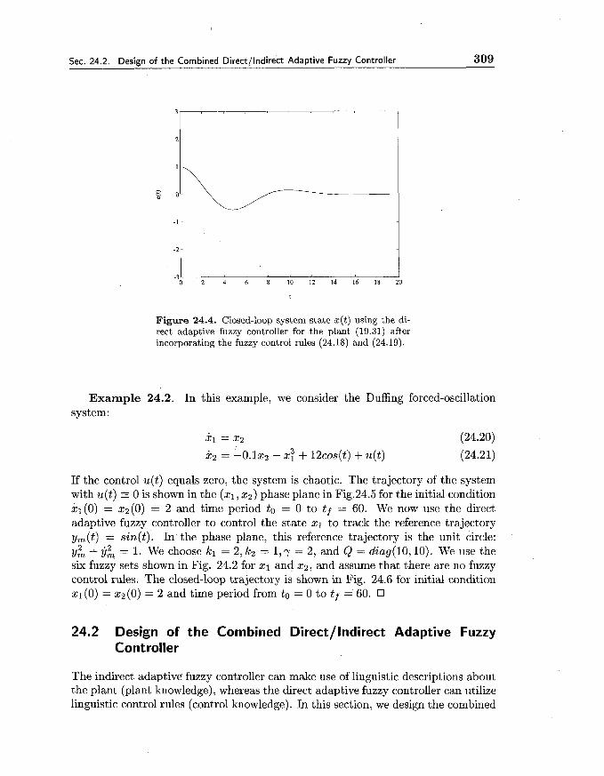
Sec. 24.2. Design of the Combined Directflndirect Adaptive Fuzzy Controller 309
Figure 24.4. Closed-loop system state x ( t ) using the di- rect adaptive fuzzy controller for the plant (19.31) after incorporating the fuzzy control rules (24.18) and (24.19).
Example 24.2. In this example, we consider the Duffing forced-oscillation system:
If the control u(t) equals zero, the system is chaotic. The trajectory of the system with u(t) 0 is shown in the (xl, x2) phase plane in Fig.24.5 for the initial condition xl(0) = x2(0) = 2 and time period to = 0 to tf = 60. We now use the direct adaptive fuzzy controller to control the state XI to track the reference trajectory y,(t) = sin(t). In the phase plane, this reference trajectory is the unit circle: y& + y& = 1. We choose kl = 2, k2 = 1, y = 2, and Q = diag(l0,lO). We use the six fuzzy sets shown in Fig. 24.2 for xl and xz, and assume that there are no fuzzy control rules. The closed-loop trajectory is shown in Fig. 24.6 for initial condition XI (0) = x2 (0) = 2 and time period from to = 0 to tf = 60.
24.2 Design of the Combined Directllndirect Adaptive Fuzzy Controller
The indirect adaptive fuzzy controller can make use of linguistic descriptions about the plant (plant knowledge), whereas the direct adaptive fuzzy controller can utilize linguistic control rules (control knowledge). In this section, we design the combined
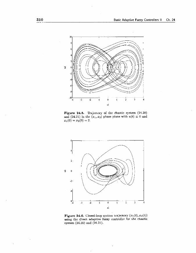
310 Basic Adaptive Fuzzv Controllers II Ch. 24
Figure 24.5. Trajectory of the chaotic system (24.20) and (24.21) in the (x1,x2) phase plane with u(t ) = 0 and x1(0) = x2(0) = 2.
Figure 24.6. Closed-loop system trajectory (XI (t), xz (t)) using the direct adaptive fuzzy controller for the chaotic system (24.20) and (24.21).

Sec. 24.2. Design o f the Combined Directllndirect Adaptive Fuzzy Controller 311
indirectldirect adaptive fuzzy controller that can incorporate both types of linguistic information.
24.2.1 Problem Specification
Consider the plant (24.1)-(24.2). For simplicity, assume that b = 1. Suppose that the following three pieces of information are available:
Information 1: We know an approximate model of the plant; that is, we are given a function f , which is an estimate of the f in (24.1).
Information 2: We are given a set of fuzzy IF-THEN rules describing the difference f - f̂ under various conditions; that is, we have
IF XI i s S{ and . - . and x, i s s;, THEN f - j i s ~j (24.22)
where S{ and Ej are fuzzy sets in R, and j = 1,2, ..., L,.
a Information 3: We are given L, fuzzy IF-THEN rules in the form of (24.3), which describe recommended control actions under various conditions.
Information 1 represents mathematical knowledge about the plant (obtained according to system configuration and physical laws), and Informations 2 and 3 are linguistic knowledge about the approximate mathematical model and the control actions, respectively. Our objective is to combine these three pieces of information into a controller and to design an adaptation law for the adjustable parameters in the controller, such that the closed-loop output y(t) follows the ideal output y,(t).
24.2.2 Design of the Fuzzy Controller
Let k and e be as defined in Subsection 23.2.2. If f (x) is known, then we know from Subsection 23.2.2 that the optimal control
u* = - f (x) + yk) + kTe (24.23)
applied to (24.1) (with b = 1) guarantees y(t) + y,(t). Let fl(xl6'1) be a fuzzy system constructed from the rules including (24.22), then the best estimate of f (x), based on Informations 1 and 2, is
Hence, to utilize Informations 1 and 2, we should use the controller
Since Information 3 consists of a set of fuzzy control rules, to use it we should consider the controller
~3 = . z ~ D ( x ~ ~ D ) (24.26)
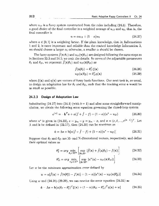
312 Basic Adaptive Fuzzy Controllers I1 Ch. 24
where u~ is a fuzzy system constructed from the rules including (24.3). Therefore, a good choice of the final controller is a weighted average of ul2 and us, that is, the final controller is
u = aul2 + (1 - a)u3 (24.27)
where a E [O, 11 is a weighting factor. If the plant knowledge, that is, Informations 1 and 2, is more important and reliable than the control knowledge Information 3, we should choose a larger a ; otherwise, a smaller a should be chosen.
The fuzzy systems f(xl0l) and u~ ( ~ 1 0 ~ ) are designed following the same steps as in Sections 23.2 and 24.1; we omit the details. In terms of the adjustable parameters BI and OD, we represent f(xl0I) and U D ( X ~ ~ D ) as
where [(x) and ~ ( x ) are vectors of fuzzy basis functions. Our next task is, as usual, to design an adaptation law for 81 and 00, such that the tracking error e would be as small as possible.
24.2.3 Design of Adaptation Law
Substituting (24.27) into (24.1) (with b = 1) and after some straightforward manip- ulation, we obtain the following error equation governing the closed-loop system
where u* is given in (24.23), e = y, - y = y, - x, and e = (e, 6, ..., e(n-l))T. Let A and b be defined in (23.17), then (24.30) can be rewritten as
Suppose that BI and OD are M- and N-dimensional vectors, respectively, and define their optimal values as
0; = arg min [ sup 1 f (x) + f(xl01) - f (x) I] OrERM XER"
0 h = a r g min sup I U * ( X ) - - U D ( ~ ~ ~ D ) ~ ~ D E R ~ I XERn
Let w be the minimum approximation error defined by
w = a[f^(x) + f (~10;) - f (x)] + (1 - a)[u* (x) - ~D(xl0h) l (24.34)
Using w and (24.28)-(29.29), we can rewrite the error equation (24.31) as
6 = he + b[a(dr - B;)~J(x) + (1 - a ) ( 0 ~ - B ~ ) ~ ~ ( X ) + W] (24.35)

Sec. 24.2. Design of the Combined Directllndirect Adaptive Fuzzy Controller 313
Consider the Lyapunov function candidate
where P > 0 satisfies the Lyapunov equation (23.25), and yl, 7 2 are positive con- stants. Using (24.35) and (23.25), we have
Therefore, if we choose the adaptation law
then we have
Since w is the minimum approximation error, (24.40) is the best we can get.
In summary, the combined directlindirect adaptive fuzzy control system is shown in Fig.24.7. We see from the figure that Information 1 is directly used ,in the controller, and Informations 2 and 3 are incorporated throught the initial parameters eI (0) and OD (0) , respectively.
24.2.4 Convergence Analysis
Up to this point, we have developed the basic schemes of indirect, direct, and com- bined indirectldirect adaptive fuzzy controllers. We used the Lyapunov synthesis approach to design these adaptive fuzzy controllers, so that they are intuitively appealing. However, we did not analyze the performance of the resulting adaptive fuzzy control systems in detail. There are two fundamental issues in performance analysis: stability and convergence, where by stability we mean the boundedness of the variables involved (states, parameters, etc.), and by convergence we mean the convergence of the tracking error to zero. We now show in the following theorem that if the fuzzy control system in Fig. 24.7 is stable, then under mild conditions the tracking error will converge to zero. In the next chapter, we will develop approaches to achieve stability.
Theorem 24.1. Consider the combined indirectldirect adaptive fuzzy control system in Fig. 24.7. If the state x, the parameters 01 and 80 , and the minimum approximation error w are bounded, then:
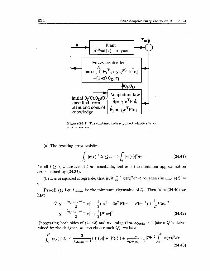
314 Basic Adaptive Fuzzy Controllers I I Ch. 24
I FUZZY controller I I
Adaptation law
fiant and control knowledge
Figure 24.7. The combined indirectldirect adaptive fuzzy control system.
(a) The tracking error satisfies
for all t 2 0, where a and b are constants, and w is the minimum approximation error defined by (24.34).
(b) If w is squared integrable, that is, if Som lw(t)12dt < oo, then limt-tm le(t) 1 = 0.
Proof: (a) Let XQrnin be the minimum eigenvalue of Q. Then from (24.40) we have
Integrating both sides of (24.42) and assuming that XQrnin > 1 (since Q is deter- mined by the designer, we can choose such Q), we have
Sec. 24.3. Summary and Further Readings 315
Define a = (Iv(o) I + suptto lv(t) 1 ) and b = A I P b 1 2 , X Q T ~ ~ ~ - 1 (24.43) becomes (24.41). (Note that sup,,, - IV(t) 1 is finite since e, Or -8; and OD - 8; are all bounded by assumption.)
(b) If w is squared integrable, then from (24.41) we conclude that e is also squared integrable. Since all the variables in the right-hand side of (24.35) are bounded by assumption, we have that e is also bounded. Using the Barbalat's Lemma (Sastry and Bodson [1989]) (If e is squared integrable and bounded and e is bounded, then 2imt,,le(t)l = 0), we have limt,,le(t)l = 0.
Using the same ideas as in the proof of Theorem 24.1, we can prove that if all the variables in the indirect and direct adaptive fuzzy control systems in Figs. 23.2 and 24.1 are bounded and the minimum approximation errors are squared integrable, then the tracking errors will converge to zero.
24.3 Summary and Further Readings
In this chapter we have demonstrated the following:
How to design the direct adaptive fuzzy controller.
How to combine the approximate mathematical model, linguistic model de- scription, and linguistic control rules into a single adaptive fuzzy controller (the combined indirectldirect adaptive fuzzy controller).
Convergence analysis of the adaptive fuzzy control systems.
The materials in this chapter are taken from Wang [1994a], where more simula- tion results can be found. Other adaptive fuzzy control approaches can be found in, for example, Spooner and Passino [1995], Johansen [1994], and Vandegrift, Lewis, Jagannathan, and Liu [1995].
24.4 Exercises
Exercise 24.1. Consider the indirect adaptive fuzzy control system in Fig. 23.2 and show that the tracking error of the closed-loop system satisfies the bound (24.41).
Exercise 24.2. Show that the tracking error of the direct adaptive fuzzy control system in Fig. 24.1 satisfies the bound (24.41).
Exercise 24.3. Suppose Informations 1 and 2 in Section 24.2 are replaced by a set of fuzzy IF-THEN rules describing the unknown function f . Combine these rules with Information 3 into an adaptive fuzzy controller.
Exercise 24.4. Suppose that the parameters in the membership functions p I ; A i
in the fuzzy controller U D of (24.6) are also adjustable parameters (so that the u~

316 Basic Adaptive Fuzzy Controllers I I Ch. 24
cannot be linear in the parameters 6 as in (24.7)). Design a direct adaptive fuzzy controller in this case.
Exercise 24.5. Repeat the simulation in Fig. 24.3 with different initial condi- tions.
Exercise 24.6. Simulate the combined indirectldirect adaptive fuzzy controller for the systems in Examples 24.1 and 24.2.

Chapter 25
Advanced Adaptive Fuzzy Controllers I
In Chapters 23 and 24, we developed the basics of indirect, direct, and combined indirectldirect adaptive fuzzy controllers. The idea was to use the Lyapunov syn- thesis approach and the certainty equivalent principle. Although we did not provide much theoretical analysis, we proved in Theorem 24.1 that if all the variables in- volved are bounded and the minimum approximation error is squared integrable, the tracking error will converge to zero. Therefore, the key problems are: (i) how to guarantee the boundedness of all the variables, and (ii) how to make the minimum approximation error squared integrable. Since the fuzzy systems are universal ap- proximators, we can make the minimum approximation error arbitrarily small by using more rules to construct the fuzzy systems. The main objective of this chapter is to solve the first problem. In Sections 25.1 and 25.2, we will use supervisory control and parameter projection to guarantee the boundedness of the states and the parameters, respectively.
25.1 State Boundedness By Supervisory Control
25.1.1 For Indirect Adaptive Fuzzy Control System
Consider the basic indirect adaptive fuzzy control system in Fig. 23.2; that is, the plant is (23.1)-(23.2), the controller is (23.7) with the fuzzy systems f* and given by (23.12) and (23.13), and the adaptation law is (23.27)-(23.28). Our task now is t o make the state x bounded.
We use the supervisory control idea in Chapter 20 for this task. Specifically, we append a supervisory controller us on top of the basic controller u~ of (23.7), so that the controller now becomes
The us should be designed to: (i) guarantee the boundedness of x, and (ii) operate
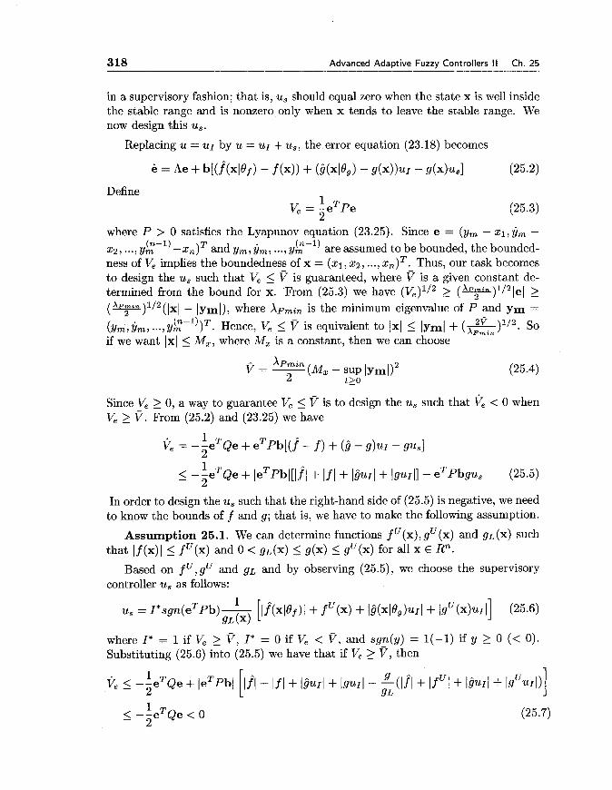
318 Advanced Adaptive Fuzzy Controllers II Ch. 25
in a supervisory fashion; that is, us should equal zero when the state x is well inside the stable range and is nonzero only when x tends to leave the stable range. We now design this us.
Replacing u = u~ by u = u l + us, the error equation (23.18) becomes
Define 1
V - -eTpe e - 2
(25.3)
where P > 0 satisfies the Lyapunov equation (23.25). Since e = (y, - xl, y, - (n-1) T
2 2 , ..., Ym -xn) and y,, $,, ..., y2-l) are assumed to be bounded, the bounded- ness of Ve implies the boundedness of x = (xl , x2, . . . , x , ) ~ . Thus, our task becomes to design the us such that Ve 5 V is guaranteed, where V is a given constant de- termined from the bound for x. From (25.3) we have (ve)ll2 2 (*)1/21e1 > (*)1/2(1~1 - Iyml), where Xpm,, is the minimum eigenvalue of P and y m =
(Y,, yml ..., yg-l))T. Hence, V, 5 V is equivalent to 1x1 5 lyml + ( Z ) l l 2 . X ~ r n z n SO if we want 1x1 5 M,, where M, is a constant, then we can choose
Since Ve 2 0, a way to guarantee Ve 5 V is to design the us such that < 0 when V, 2 V . From (25.2) and (23.25) we have
1 Ve = -5eT&e + eTpb[(.f - f ) + (6 - g ) u ~ - gas]
1 5 - z e T ~ e + e T ~ b l [ l f l + I f / + ~ u ~ l + / g ~ ~ I ] - e T ~ b g u s (25.5)
In order to design the us such that the right-hand side of (25.5) is negative, we need to know the bounds of f and g; that is, we have to make the following assumption.
Assumption 25.1. We can determine functions f U(x), gU (x) and gL (x) such that I f (x) 1 5 f (x) and 0 < gL (x) 5 g(x) 5 gU(x) for all x E Rn.
Based on fU ,gU and g~ and by observing (25.5), we choose the supervisory controller us as follows:
where I* = 1 if Ve 2 v, I* = 0 if Ve < V, and sgn(y) = 1(-1) if y 2 0 (< 0). Substituting (25.6) into (25.5) we have that if Ve 2 V, then

Sec. 25.1. State Boundedness By Supervisory Control 319
where we assume e # 0 since this is natural under Ve 2 V . Consequently, using the control (25.1) with us given by (25.6), we can guarantee that Ve 5 V, which, when ?' is chosen according to (25.4), guarantees 1x1 5 Mx for any given constant Mx .
Because of the indicator function I*, us is nonzero only when Ve > V, therefore us is a supervisory controller. That is, if the closed-loop system with the fuzzy controller ur of (23.7) is well-behaved in the sense that the error is within the constraint set (that is, Ve 5 V or equivalently 1x1 5 M,), then the supervisory controller us is idle. On the other hand, if the system tends to be unstable (that is, Ve 2 V), then the supervisory controller u, takes action to force Ve 5 V.
25.1.2 For Direct Adaptive Fuzzy Control System
Consider the basic direct adaptive fuzzy control system in Fig.24.1, where the pro- cess is modeled by (24.1)-(24.2), the controller is the fuzzy system (24.7), and the adaptation law is given by (24.16). Our task now is to design a supervisory con- troller us on top of the fuzzy controller u ~ , such that the state x is guaranteed to be bounded.
Let the control be u = u ~ ( x l 6 ) + u,(x) (25.8)
and define the ideal control u* as in (23.5) (with g(x) = b). Substituting (25.8) into (24.1) and after rearrangement, we obtain the closed-loop error equation
where A and b are the same as in (24.9). Defining the Lyapunov function candidate Ve as in (25.3) and using (25.9) and (23.25), we have
In order to design us such that ve < 0, we have to make the following assumption, which is essentially the same as Assumption 25.1.
Assumption 25.2. We can determine a function f U(x) and a constant bL such that I f (x) 1 5 f (x) and 0 < b~ 5 b.
By observing (25.10) and (23.5), we design the supervisory controller us as follows:
where the indictor function I* is the same as that in (25.6); that is, I* = 1 if V, > V, I* = 0 if V, < v , where v is determined according to the bound of x as

320 Advanced A d a ~ t i v e Fuzzv Controllers I I Ch. 25
in (25.4). Substituting (25.11) and (23.5) into (25.10) and considering the I* = 1 case, we have
Therefore, using the supervisory controller us, we can guarantee that V, < V , from which we have 1x1 5 Mz if we choose V according to (25.4).
The design of supervisory controller for the combined indirectldirect adaptive fuzzy control system is left as an exercise.
25.2 Parameter Boundedness By Projection
25.2.1 For Indirect Adaptive Fuzzy Control System
Using the basic adaptation law (23.27)-(23.28), we cannot guarantee that the pa- rameters O f and Og are bounded. If O f diverges to infinity, then the fuzzy system f ( x 1 0 ~ ) will steadily increase and result in an unbounded control u l ; this is clearly unacceptable. Therefore, to develop a stable system (in the sense that all variables are bounded), we must modify the adaptation law such that the parameters are bounded.
Let the constrain sets Rf and Rg for O f and 8, be defined as
where p, and q, are as defined in Subsection 23.2.2, and M f , E and Mg are constants. We require l0,l to be bounded from below by 6 > 0 because from (23.7) we see that g = O T r l must be nonzero. We now modify the basic adaptation law (23.27)-(23.28) to guarantee O f E R and Og E Rg .
The basic idea is the following: if the parameter vector is in the interior of the constraint set or on the boundary but moving toward the inside of the constraint set, then use the basic adaptation law (23.27)-(23.28); if the parameter vector is on the boundary of the constraint set but moving toward the outside of the constraint set, then project the gradient of the parameter vector onto the supporting hyper- plane; see Fig.25.1. Specifically, the modified adaptation law with projection for the indirect adaptive fuzzy system is given as follows:

Sec. 25.2. Parameter Boundedness By Projection 321
A supporting hyperplane
Figure 25.1. Illustration of the projection algorithm.
Adaptation Law with Projection:
For O f , use
-%eTpb[(x) if ( ( O f ( < M f ) ~ ~ ( ( O f ( = M f a n d 0, = eTpb0?[(x) 2 0)
~ { - - y ~ e ~ ~ b [ ( x ) ) if (let/ = Mf and eTpb0:[(x) < 0) (25.15)
where the projection operator P{*) is defined as
For 09, use
Whenever an element Ogi of 0, equals E , use
where qi(x) is the ith component of ~ ( x ) .

322 Advanced Adaptive Fuzzy Controllers II Ch. 25
Otherwise, use
- y 2 e T P b r l ( x ) u ~ i f ( l O g l < M g ) or ( l O g l = M g and eg = e T ~ b O T r l ( x ) u r 2 0 )
~ { - y ~ e ~ ~ b ~ ( x ) u ~ ) i f ( l O g l = M g and e T ~ b O T v ( x ) u I < 0 ) (25.18)
where the projection operator P { * ) is defined as
The following theorem shows that the modified adaptation law (25.15)-(25.19) guarantees that O f E R f and 8, E 0,.
T h e o r e m 25.1. Let the constraint sets R f and Rg be defined in (25.13) and (25.14). If the initial values of the parameters satisfy O f ( 0 ) E O f and 8, ( 0 ) E Rg , then the adaptation law (25.15)-(25.19) guarantees that O f ( t ) E R f and 8, ( t ) E Rg for all t 2 0.
P r o o f : To prove lof 1 5 Mi , let Vf = ; O f T O f . If the condition in the first line of (25.15) is true, we have either lof 1 < M f or vf = -" ieT~bBfT((x) 5 0 when lof 1 = M f ; hence, we have [ O f 1 5 M f in this case. If the condition in the second line of (25.15) is true, we have / O f 1 = M f and vf = -y1eTPbOfTt(x) +
eTef T y l e T P b h O f <(x) = 0 ; hence, lof 1 5 M f in this case. Since the initial 10f(0)l 5 M f , we have lof (t)l 5 M f for all t 2 0.
Using the same method, we can prove that 10g(t)l 5 M g for all t 2 0. To show J O g J > E, we see from (25.17) that if Ogi = 6 , then egi > 0 ; hence, we always have Ogi > E which guarantees lO,l > E.
25.2.2 For Direct Adaptive Fuzzy Control System
The idea is the same. Let the constraint set for the O in the direct adaptive fuzzy controller (24.7) be
RD = (6' E R Ily=,mi I 101 5 M ~ ) (25.20)
The modified adaptation law with projection is
yeTpnE(x) i f (101 < M D ) or (101 = M D and eTpnOTS(x) 2 0 ) P{yeTpnE(x ) ) if (16) = M D and eTpaOTE(x) < 0 )
(25.21) where the projection operator is defined as
The following theorem shows the boundedness of the parameters.
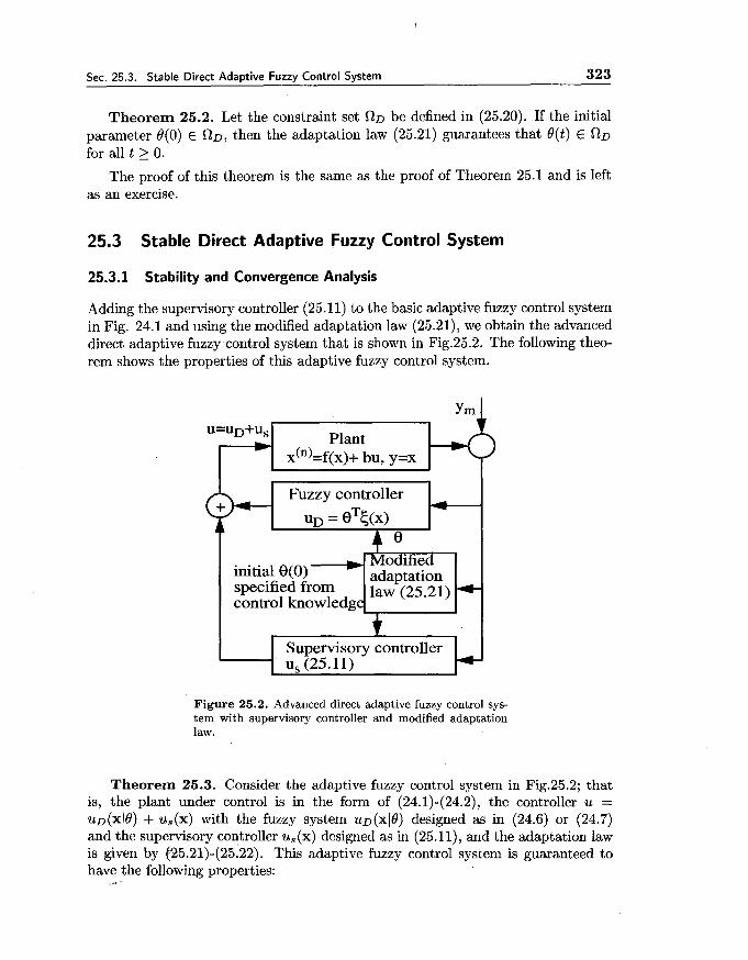
Sec. 25.3. Stable Direct Adaptive Fuzzy Control System 323
Theorem 25.2. Let the constraint set RD be defined in (25.20). If the initial parameter O(0) E C I D , then the adaptation law (25.21) guarantees that O ( t ) E OD for all t 2 0 .
The proof of this theorem is the same as the proof of Theorem 25.1 and is left as an exercise.
25.3 Stable Direct Adaptive Fuzzy Control System
25.3.1 Stability and Convergence Analysis
Adding the supervisory controller (25.11) to the basic adaptive fuzzy control system in Fig. 24.1 and using the modified adaptation law (25.21), we obtain the advanced direct adaptive fuzzy control system that is shown in Fig.25.2. The following theo- rem shows the properties of this adaptive fuzzy control system.
u=uD+Us Plant
x(~)=~(x)+ bu, y=x
specified from control knowledg
Figure 25.2. Advanced direct adaptive fuzzy control sys- tem with supervisory controller and modified adaptation law.
Theorem 25.3. Consider the adaptive fuzzy control system in Fig.25.2; that is, the plant under control is in the form of (24.1)-(24.2) , the controller u = u ~ ( x 1 0 ) + u s ( x ) with the fuzzy system u o ( x J 0 ) designed as in (24.6) or (24.7) and the supervisory controller us (x) designed as in (25.11), and the adaptation law is given by (25.21)-(25.22). This adaptive fuzzy control system is guaranteed to have the following properties:

324 Advanced Adaptive Fuzzy Controllers I1 Ch. 25
(a) All the parameters and states are bounded, that is,
where MD and MZ are constants, and the that determined the I* in us is chosen according to (25.4).
(b) The tracking error e is bounded by the minimum approximation error w (defined in (24.11)) according to
where a and b are constants.
(c) If w is squared integrable, that is, if Jr Iw(t)12dt < co, then limt-toole(t)l = 0.
Proof: (a) (25.23) follows from Theorem 25.2, and (25.24) is obtained from (25.12) (which shows V, 5 V) and (25.4) (which shows that V, < V is equivalent to Ix(t)l I Mx).
(b) With the supervisory controller us(x(0) added, the error equation (24.12) becomes
6 = h e + b(0* - O ) ~ C ( X ) - bw - bu,(x) (25.26)
Considering the Lyapunov function candidate V of (24.13) and using (25.26), we have
Substituting the adaptation law (25.21) into (25.27) and letting I; = 1 indicate that the condition in the second line of (25.21) is true and Ig* = 0 indicate the other cases, we have
We now show that the second term in the right-hand side of (25.28) is nonpositive. If I,* = 0, the conclusion is trivial. Let Ig* = 1, which means that 101 = MD and eTpnBT[(x) < 0, we have (0* - = !j(10*I2 - l0I2 - 16 - Q*l2) < 0 since 101 = MD 2 l0*l Therefore, (25.28) is simplified to

Sec. 25.3. Stable Direct Adaptive Fuzzy Control System 325
Since the supervisory controller u,(x) of (25.11) has the same sign as eTpb , we obtain from (25.29) that
where XQrnin is the minimum eigenvalue of Q and we assume XQrnin > 1. Integrat- ing both sides of (25.30), we obtain
2 IpnbI2, (25.31) becomes Define a = =(lV(O)l +supttolV(t)1) and b = -- X Q ~ ~ ~ - 1
(25.25).
(c) If w E L2, then from (25.25) we have e E L2. Because all the variables in the right-hand side of (25.26) are bounded, we have e E L,. Using Barbalat's Lemma (Sastry and Bodson [1989]: if e E L2 n L, and e E L,, then limt,,le(t)l = O), we have limt+, le(t) 1 = 0.
25.3.2 Simulations
Example 25.1. Consider the same situation as in Example 24.1, except that the supervisory controller u, of (25.11) and the modified adaptation law (25.21) is used. We still use the six fuzzy sets as shown in Fig. 24.2 and choose the initial di(O)'s randomly in [-2,2]. The difference is that we require 1x1 5 Mz = 1.5 and 10) 5 MD = 10. With initial x(0) = 1, the simulation result is shown in Fig. 25.3. From Fig. 25.3 we see that the supervisory controller indeed forced the state to be within the constraint set.
Example 25.2. The same as Example 24.2 except that the supervisory con- troller is added and the adaptation law is modified. Consider the same condition as in Fig. 24.6, except that we require 1x1 2 Mz = 3. Fig. 25.4 shows the simulation result for this case. We see again that the supervisory controller did its job.

326 Advanced Adaptive Fuzzy Controllers II Ch. 25
Figure 25.3. Closed-loop system state x(t) = e ( t ) for Example 25.1.
Figure 25.4. Closed-loop system trajectory in the xi- xz phase plane for Example 25.2.

Sec. 25.4. Summary and Further Readings 327
25.4 Summary and Further Readings
In this chapter we have demonstrated the following:
How to design the supervisory controller to guarantee the boundedness of the states.
How to modifiy the basic adaptation laws through projection such that the parameters are guaranteed to be bounded.
The stable direct adaptive fuzzy control scheme and its properties.
Projection algorithms were studied in Luenberger [I9691 and Luenberger [1984]. There are other methods to guarantee the boundedness of the parameters, such as dead-zone (Narendra and Annaswamy [I9891 and Sastry and Bodson [1989]), 6-modification (Ioannou and Kokotovic [1983]), and 6-modification (Narendra and Annaswamy [1989]). The stable direct adaptive fuzzy controller in this chapter was taken from Wang [1993].
25.5 Exercises
Exercise 25.1. Design a supervisory controller for the combined indirectldirect adaptive fuzzy control system developed in Section 24.2, such that the states of the closed-loop system are bounded. Prove that your supervisory controller achieves the objective.
Exercise 25.2. Modify the adaptation law by introducing projection for the combined indirectldirect adaptive fuzzy control system in Section 24.2, such that the parameters are bounded. Prove that your adaptation law achieves the objective.
Exercise 25.3. Show that (25.16) is indeed a projection operator; that is, prove that:
(a) ~ { - - y l e ~ P b t ( x ) } is orthogonal to P{-yleT~b~(x))-(-y~eT~b~(x)), and
(b) ~ { - - y I e ~ P b t ( x ) ) lies on the supporting hyperplane of Of at the point B f .
Exercise 25.4. Prove Theorem 25.2.
Exercise 25.5. Repeat the simulation in Example 25.1 with x(0) = 1.4.
Exercise 25.6. Repeat the simulation in Example 25.2 with Mz = 4.

Chapter 26
Advanced Adaptive Fuzzy Controllers I I
26.1 Stable Indirect Adaptive Fuzzy Control System
26.1.1 Stability and Convergence Analysis
Continuing with Chapter 25, we add the supervisory controller u,(x) of (25.6) to the basic indirect adaptive fuzzy controller of (23.7) and change the adaptation law to (25.15)-(25.19). This advanced indirect adaptive fuzzy control system is shown in Fig. 26.1. The following Theorem shows the stability and convergence properties of this system.
Theorem 26.1. Consider the indirect adaptive fuzzy control system in Fig. 26.1; that is, the plant is (23.1)-(23.2), the control u = ur + us where ul is given by (23.7) and us is given by (25.6), and the adaptation law is (25.15)-(25.19). This adaptive fuzzy control system is guaranteed to have the following properties:
(a) All the parameters and states are within the constraint sets, that is,
where Rf and 0, are defined in (25.13) and (25.14), respectively, and the in the I* of us is chosen according to (25.4).
(b) The tracking error e satisfies (25.25), where w is defined in (23.21) and a, b are constants.
(c) If w is squared integrable, then Eimt+,(e(t)( = 0.
The proof of this Theorem follows the same arguments as in the proof of Theorem 25.3, and is left as an exercise.

Sec. 26.1. Stable Indirect Adaptive Fuzzy Control System 329
Fuzzy controller 4
UI of (23.7)
u=ul+us +
Figure 26.1. Advanced indirect adaptive fuzzy control system with supervisory controller and modified adaptation
Plant
Jn)=f(x)+ g(x)u, y=q
law.
26.1.2 Nonlinear Parameterization
In the fuzzy controller of the indirect adaptive fuzzy control systems in Figs. 23.2 and 26.1, the fuzzy systems f(xl0 f ) and ij(x10,) are linearly parameterized, as shown in (23.12) and (23.13). To achieve this linear parameterization, the IF- part membership functions must be fixed and the adaptation laws only adjust the centers Of and 0, of the THEN-part fuzzy sets. In order for the fuzzy systems f"(x1ef) and j(xl0,) to be well-behaved at any x in the domain of interest, the IF- part membership functions have to cover the whole domain. Therefore, the numbers of rules in the fuzzy systems f ( x 1 0 ~ ) and j(xl0,) increase exponentially with the dimension of x. One way to reduce the number of rules is to allow the IF-part membership functions also to change during the adaptation procedure, so that the same rule can be used to cover different regions of the state space at different times.
Specifically, we choose f(xlef) and ij(xl0,) to be the fuzzy systems in the form of (9.6) (fuzzy systems with product inference engine, singleton fuzzifier, center- average defuzzifier, and Gaussian membership functions), that is,

330 Advanced Adaptive Fuzzy Controllers I I Ch. 26
where Of and 8, are the collections of the parameters ($, 51fi, oii) and (gk, 5ii, aii), respectively. Let the optimal parameters 8; and 8; be defined as in (23.19) and (23.20). In order to use the same approach as in Subsection 23.2.3 to design the adaptation law, we take the Taylor series expansions of f(xl8 j) and i(xl8;) around Of and 8, and obtain
where O(lOf - 8; 1 2 ) and O(l8, - 8; 12) are higher-order terms.
Substituting (26.5)-(26.6) into (23.22), we obtain the error equation
where = + o ( p f - e;12) + o(18 , - 8g12) (26.8)
and w is defined in (23.21). Comparing (26.7) with (23.23) we see that we can use the same approach in Subsection 23.2.3 to design the adaptation law-just replacing
F(x) by Bf , q(x) by Bgk;rg) , and w by u; that is, the adaptaion law in this case is
The (advanced) adaptation law with projection can be developed in the same way as in the linear parameterization cases.
To implement the adaptation law (26.9)-(26.10), we must know how to compute
Bf(X'efl and @&Yg). Fmm Chapter 13 we know that these two derivatives can be 00,
af(x'ef) is computed computed using the back-propagation algorithm. Specifically, from

Sec. 26.2. Adaptive Fuzzy Control o f General Nonlinear Systems 331
where
ag(x'eg) can be computed using the same algorithm (26.11)-(26.15) with f replaced a09
by g.
26.2 Adaptive Fuzzy Control of General Nonlinear Systems
The adaptive fuzzy controllers developed up to this point were designed for nonlinear systems in the canonical form (23.1)-(23.2). In practice, however, many nonlinear systems may not be represented in the canonical form. In general, a single-input- single-output continuous-time nonlinear system is described by
where x E Rn is the state vector, u E R and y E R are the input and output of the system, respectively, and F and h are nonlinear functions. In this section, we consider the general nonlinear system (26.16); our objective is to make the output y ( t ) track a desired trajectory y,(t).
Comparing (26.16) with the canonical form (23.1)-(23.2), we see that a difficulty with this general model is that the output y is only indirectly related to the input u, through the state variable x and the nonlinear state equation; on the other hand, with the canonical form the output (which equals the first state variable) is directly related to the input. Therefore, inspired by the results of Chapters 23-25, we might guess that the difficulty of the tracking control for the general nonlinear system (26.16) can be reduced if we can find a direct relation between the system output y and the control input u. Indeed, this idea constitutes the intuitive basis for the so-called input-output linearization approach to nonlinear controller design (Isidori [1989]).
Input-output linearization is an approach to nonlinear controller design that has attracted a great deal of interest in the nonlinear control community in recent years. This approach differs entirely from conventional linearization (for example, Jacobian
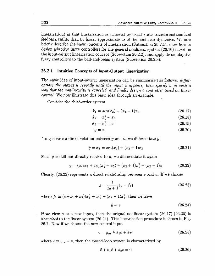
332 Advanced Adaptive Fuzzy Controllers I I Ch. 26
linearization) in that linearization is achieved by exact state transformations and feedback rather than by linear approximations of the nonlinear dynamics. We now briefly describe the basic concepts of linearization (Subsection 26.2.1), show how to design adaptive fuzzy controllers for the general nonlinear system (26.16) based on the input-output linearization concept (Subsection 26.2.2), and apply these adaptive fuzzy controllers to the ball-and-beam system (Subsection 26.2.3).
26.2.1 Intuitive Concepts of Input-Output Linearization
The basic idea of input-output linearization can be summarized as follows: differ- entiate the output y repeatly until the input u appears, then specify u i n such a way that the nonlinearity is canceled, and finally design a controller based o n linear control. We now illustrate this basic idea through an example.
Consider the third-order system
To generate a direct relation between y and u, we differentiate y
Since y is still not directly related to u, we differentiate it again
Clearly, (26.22) represents a direct relationship between y and u. If we choose
where fl E (cosx2 + 23) (2: + 23) + (x2 + I)$!, then we have
If we view v as a new input, then the orignal nonlinear system (26.17)-(26.20) is linearized to the linear system (26.24). This linearization procedure is shown in Fig. 26.2. Now if we choose the new control input
where e y, - y , then the closed-loop system is characterized by
e + k l & + k2e = 0 (26.26)

Sec. 26.2. Adaptive Fuzzy Control of General Nonlinear Systems 333
Nonlinear system (26.17)-(26.20) 5
fl I
x2+ 1
Linearized system
Figure 26.2. Diagram of the linearized system for the nonlinear system (26.17)-(26.20).
If we choose kl and k2 such that all roots of s2 + kls+k2 = 0 are in the open left-half complex plane, then we have limt,,e(t) = 0, which is our control objective.
If we need to differentiate the output of a system r times to generate a direct relationship between the output y and the input u, this system is said to have relative degree r. Thus, the system (26.17)-(26.20) has relative degree 2. It can be shown formally that for any controllable system of order n, it will take at most n differentiations of any output for the control input to appear; that is, the relative degree of any n'th-order controllable system is less than or equal to n.
At this point one might feel that the tracking control problem for the nonlin- ear system (26.17)-(26.20) has been solved with control law (26.23) and (26.25). However, one must realize that (26.26) only accounts for part of the whole sys- tem because it has only order 2, while the whole system has order 3. Therefore, a part of the system dynamics has been rendered "unobservable" in the input-output linearization. This part of the system is called the internal dynamics, because it can- not be seen from the external input-output relationship (26.24). For the preceding example, the internal dynamics are represented by
which is obtained by substituting (26.23) and (26.25) into (26.19). If these internal dynamics are stable in the sense that the state x3 is bounded, our tracking control problem has indeed been solved. Otherwise, we have to redesign the control law.

334 Advanced Adaptive Fuzzy Controllers I1 Ch. 26
26.2.2 Design of Adaptive Fuzzy Controllers Based on Input-Output Lineariza- tion
From the last subsection we see that the input-output linearization approach re- quires that the mathematical model of the system is known, because otherwise the differentiation procedure cannot be performed. In our problem, however, the nonlinear functions F and h in (26.16) are assumed to be unknown. How can we generalize the approach of input-output linearization to our problem?
First, inspired by the certainty equivalent controller in Chapter 23, one may think to replace the F and h by fuzzy systems and then develop an adaptation law to adjust the parameters of the fuzzy systems to make them approximate F and h. Indeed, this is a valid idea. However, this approach will result in a very complicated adaptive control system. The reason is that, although the original fuzzy systems for approximating F and h are linear in their parameters, the differentiations cause these parameters to appear in a nonlinear fashion in later stages of the differentiation procedure. Therefore, we do not take this approach.
Our approach is based on the following consideration: from the last subsection we see that the control design (26.23) is based only on the final system (26.22) in the differentiation procedure, the intermediate system (26.21) is not directly used; therefore, instead of approximating the F and h by fuzzy systems, we approximate the nonlinear functions in the final equation of the differentiation procedure by fuzzy systems. We then can develop an adaptation law to adjust the parameters of the fuzzy systems to make y track y,. To give the details in a formal way, we need the following assumption.
Assumption 26.1. We assume that: (i) the nonlinear system (26.16) has relative degree r , (ii) the control u appears linearly with respect to y(T), that is,
y"' = f (x) + g(x)u
where f and g are unknown functions and g(x) # 0, and (iii) the internal dynamics of the system with the following adaptive fuzzy controller are stable.
Design of Adaptive Fuzzy Controller Based on Input-Output Lin- earization:
Step 1. Determine the relative degree r of the nonlinear system (26.16) based on physical intuitions. Specifically, we analyze the physical meanings of y, y, y, ..., and determine the y(T) that is directly related to u. We will show how to do this for the ball-and-beam system in the next subsection.
Step 2. Choose the fuzzy systems f ( x 1 0 ~ ) and g(xlOg) in the form of (9.6), that is,
f(x10f) = $t(x) (26.29)
i(xl0g) = 0Fl(x) (26.30)
Sec. 26.2. A d a ~ t i v e Fuzzv Control of General Nonlinear Systems 335
Step 3. Design the controller as
where k = (k,, ..., kl)T is such that all roots of s r +klsr-l +. . .+k, = 0 are in the open left-half complex plane, and e = (e, 8, ..., e('-l))T with e = y, - y.
Step 4. Use the adaptation law
to adjust the parameters, where P and b are defined as in Chapter 23. The overall control system is the same as in Fig.23.2 except that the plant is changed to (26.16) and n is changed to r.
The controller (26.31) and adaptation law (26.32)-(26.33) are obtained by using the same Lyapunov synthesis approach as in Chapter 23. This can be done because Assumption 26.1 ensures that controlling (26.16) is equivalent to controlling (26.28).
Using the same ideas as in Chapter 25, we can add a supervisory controller to the fuzzy controller (26.31) to guarantee the boundedness of y = (y, y, ..., y(r-l))T. We also can use the projection algorithm to modify the adaptation law (26.32)-(26.33) to guarantee the boundedness of Of and 8,. If linguistic information for f and g is available, we can incorporate it into the initial Of(0) and Og(0) in the same way as in Chapter 23.
The preceding adaptive fuzzy controller is an indirect adaptive fuzzy controller. We also can develop a direct adaptive fuzzy controller using the same idea as in Chapter 24. The resulting controller is
with adaptation law e = yeTpr<(x)
where p, is defined as in Chapter 24. Similarly, we can also develop a combined indirect/direct adaptive fuzzy controller for the general nonlinear system.
26.2.3 Application to the Ball-and-Beam System
The ball-and-beam system is illustrated in Fig. 16.7 and is characterized by (16.4) and (16.5). In this subsection, we use the adaptive fuzzy controllers developed in the last subsection to control the ball position y = XI to track the trajectory y,(t) = sin(t).
336 Advanced Adaptive Fuzzy Controllers I I Ch. 26
We begin with Step 1, that is, determining the relative degree r of the ball- and-beam system based on physical intuitions. First, we realize that the control u equals the acceleration of the beam angle 0; thus, our goal is to determine which derivative of y is directly related to the acceleration of 0. Clearly, the ball position y = XI = r and the ball speed along the beam y are not directly related to v. Based on Newton's Law, the acceleration of the ball position, y, is propositional to sin(0), which is not directly related to u = 0. Therefore, 5 is not directly related to u. Because y is propositional to sin(@), g ( 3 ) is directly related to e, but not directly related to u = 0. Finally, we see that y(4) is directly related to u. Therefore, the relative degree of the ball-and-beam system equals 4.
In Step 2, we define three fuzzy sets ,uN(x~) = l / ( l + exp(5(xi + I))), ,UZ(xi) = exp(-x:) and xi) = 1/(1 + exp(-5(xi - 1))) for all zl to 24. Therefore, the dimension of Of, 0, and [(x) equals 34 = 81. Because there is no linguistic informa- tion about f and g, the initial Bf(0), and 0,(0) were chosen randomly in the interval [-2, 21.
In Step 3, we choose k = (1,4,6, 4)T, and in Step 4 we choose yl = 2 and 7 2 = 0.2. Figs. 26.3 and 26.4 show the y(t) (solid line) using this adaptive fuzzy controller along with the desired trajectory ym(t) (dashed line) for initial conditions x(0) = (1,0,0, o ) ~ and x(0) = (-1,0,O, o ) ~ , respectively.
We also simulated the direct adaptive fuzzy controller (26.34) and (26.35). We chose the [(x) to be the same as in the preceding indirect adaptive fuzzy controller. We chose y = 10. Figs. 26.5 and 26.6 show the y(t) (solid line) using this direct adaptive fuzzy controller along with the desired trajectory ym(t) for initial condi- tions x(0) -= (1,0,O, o ) ~ and x(0) = (-0.4,0,0, o ) ~ , respectively. Comparing Figs. 26.3-26.4 with Figs. 26.5-26.6 we see that the direct adaptive fuzzy controller gave better performance than the indirect adaptive fuzzy controller for this example.
l ~ e did not give a mathematically rigorous definition of relative degree in Subsection 26.2.1; therefore, the relative degree determined in this fashion can only be viewed as an intuitive relative degree. For the rigorous definition of relative degree, see Isidori [I9891 and Slotine and Li [1991].

Sec. 26.2. Adaptive Fuzzy Control of General Nonlinear Systems 337
Figure 26.3. The output y(t) (solid line) using the indi- rect adaptive fuzzy controller (26.31)-(26.33) and the de- sired trajectory y,(t) (dashed line) for the ball-and-beam system with the initial condition x(0) = (1,0,O, o ) ~ .
Figure 26.4. The output y(t) (solid line) using the indi- rect adaptive fuzzy controller (26.31)-(26.33) and the de- sired trajectory ym(t) (dashed line) for the ball-and-beam system with the initial condition x(0) = (-1,0,0, o ) ~ .
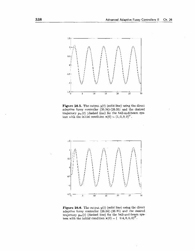
338 Advanced A d a ~ t i v e Fuzzv Controllers II Ch. 26
Figure 26.5. The output y(t) (solid line) using the direct adaptive fuzzy controller (26.34)-(26.35) and the desired trajectory y,(t) (dashed line) for the ball-and-beam sys- tem with the initial condition x(0) = (1,0,O, o ) ~ .
Figure 26.6. The output y(t) (solid line) using the direct adaptive fuzzy controller (26.34)-(26.35) and the desired trajectory yn(t) (dashed line) for the ball-and-beam sys- tem with the initial condition x(0) = (-0.4,0, O , O ) ~ .
Sec. 26.3. Summary and Further Readings 339
26.3 Summary and Further Readings
In this chapter we have demonstrated the following:
How to design adaptation laws if the IF-part membership functions of the fuzzy systems also are allowed to change during the adaptation procedure.
The basic idea of input-output linearization.
How to design adaptive fuzzy controllers for the general nonlinear systems, based on the input-output linearization concept.
Nonlinear control theory should be the principal tool in the further development of fuzzy control. There are many good books on nonlinear control, for example, Isidori [I9891 provided a rigorous treatment for nonlinear control and Slotine and Li [I9911 is more readable. The materials in this chapter are taken from Wang [1994a].
26.4 Exercises
Exercise 26.1. Prove Theorem 26.1.
Exercise 26.2. Suppose that the direct adaptive fuzzy controller uD(x16') in (24.9) is a fuzzy system in the form of (9.6) with a8 = 1. Design an adaptation law for the parameters 6' using the Lyapunov synthesis approach.
Exercise 26.3. Consider the nonlinear system
Design a state feedback controller such that the equilibrium x = 0 of the closed-loop system is locally asympototically stable.
Exercise 26.4. For the system
design an adaptive controller to track an arbitrary desired trajectory xdl (t). Assume that the state ($1, is measured, that xdl(t), xdl (t), xdl (t) are all known, and that a1 , a2 are unknown constants.
Exercise 26.5. Design a direct adaptive fuzzy controller for the general non- linear system (26.16) and simulate it for the ball-and-beam system.

340 Advanced Ada~ t i ve Fuzzv Controllers II Ch. 26

Part VI
Miscellaneous Topics
We pointed out in the Preface that in writing this book we first established the structure that a reasonable theory of fuzzy systems and fuzzy control should follow, and then filled in the details. This structure is constituted by Chapters 1-26. Because fuzzy systems and fuzzy control is a large and diversified field, some important topics were unavoidably not included in this structure. In this final part of the book (Chapters 27-31), we will study a number of important topics in fuzzy systems and fuzzy control that were not covered in Chapters 1-26. These topics are equally important as those in Chapters 1-26.
In Chapter 27, we will study perhaps the most important method in fuzzy approaches to pattern recognition-the fuzzy c-means algorithm. We will show the details of the algorithm and study its convergence properties. In Chapter 28, we will study fuzzy relation equations that are potentially very useful in fuzzy systems and fuzzy control. We will show how to obtain exact and approximate solutions to different fuzzy relation equations. In Chapter 29, we will introduce the basic arithmetic operations for fuzzy numbers, including fuzzy addition, fuzzy subtraction, fuzzy multiplication and fuzzy division. These fuzzy operations are very useful in fuzzy decision making. In Chapter 30, we will study the most important topic in fuzzy decision making-fuzzy linear programming. We will justify why fuzzy linear programming is needed and show how to solve a number of fuzzy linear programming problems. Finally, in Chapter 31, we will briefly review the basics in possibility theory and conclude the book with a discussion on fuzziness versus probability.

Chapter 27
The Fuzzy C-Means Algorithm
27.1 Why Fuzzy Models for Pattern Recognition?
Pattern recognition is a field concerned with machine recognition of meaningful reg- ularities in noisy or complex environments. In simpler words, pattern recognition is the search for structures in data. For example, Fig. 27.1 shows four cases of data structures in the plane. Observing Fig.27.1, we see that the data in each of the four cases should be classified into two groups, but the definition of a "group" is different. Specifically, the group in Fig. 27.l(a) should be classified according to the distance between data points (that is, data points with short distances among themselves should be grouped together), the group in Fig. 27.l(b) should be rec- ognized according to the connectivity of the data points (that is, data points well connected together should be classified into the same group), and the groups in Fig. 27.l(c)-(d) should be defined from a mixture of distance-based and linkage-based criteria. In pattern recognition, a group of data is called a cluster.
In practice, the data are usually not well distributed, therefore the "regularities" or "structures" may not be precisely defined. That is, pattern recognition is, by its very nature, an inexact science. To deal with the ambiguity, it is helpful to introduce some "fuzziness" into the formulation of the problem. For example, the boundary between clusters could be fuzzy rather than crisp; that is, a data point could belong to two or more clusters with different degrees of membership. In this way, the formulation is closer to the real-world problem and therefore better performance may be expected. This is the first reason for using fuzzy models for pattern recognition: the problem by its very nature requires fuzzy modeling (in fact, fuzzy modeling means more flexible modeling-by extending the zero-one membership to the membership in the interval [0,1], more flexibility is introduced).
The second reason for using fuzzy models is that the formulated problem may be easier to solve computationally. This is due to the fact that a nonfuzzy model often results in an exhaustive search in a huge space (because some key variables can only take two values 0 and l ) , whereas in a fuzzy model all the variables are continuous, so that derivatives can be computed to find the right direction for the
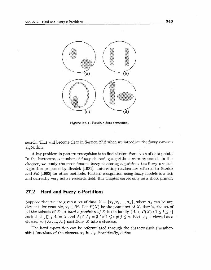
Sec. 27.2. Hard and Fuzzy c-Partitions 343
Figure 27.1. Possible data structures.
search. This will become clear in Section 27.3 when we introduce the fuzzy c-means algorithm.
A key problem in pattern recognition is to find clusters from a set of data points. In the literature, a number of fuzzy clustering algorithms were proposed. In this chapter, we study the most famous fuzzy clustering algorithm: the fuzzy c-means algorithm proposed by Bezdek [1981]. Interesting readers are referred to Bezdek and Pal [I9921 for other methods. Pattern recognition using fuzzy models is a rich and currently very active research field; this chapter serves only as a short primer.
27.2 Hard and Fuzzy c-Partitions
Suppose that we are given a set of data X = {XI, xz, ..., x,), where xk can be any element, for example, xi E R p . Let P ( X ) be the power set of X , that is, the set of all the subsets of X . A hard c-partition of X is the family {Ai E P ( X ) : 1 5 i 5 c) such that Uiz, Ai = X and Ai fl Aj = 0 for 1 < i # j 5 c. Each Ai is viewed as a cluster, so { A l , ..., A,) partitions X into c clusters.
The hard c-partition can be reformulated through the characteristic (member- ship) functions of the element xk in Ai. Specifically, define

344 The Fuzzy C-Means Algorithm Ch. 27
where xk G X, Ai E P ( X ) , i = 1,2, ..., c and k = 1,2, ..., n. Clearly, uik = 1 means that xk belongs to cluster Ai. Given the value of uik, we can uniquely determine a hard c-partition of X , and vice versa. The uik's should satisfy the following three conditions:
(27.2) and (27.3) together mean that each xk E X should belong to one and only one cluster. (27.4) requires that each cluster Ai must contain at least one and at most n - 1 data points. Collecting uik with 1 5 i 5 c and 1 < k 5 n into a c x n matrix U, we obtain the matrix representation for hard c-partition, defined as follows.
Definition 27.1. Hard c-Partition. Let X = {xl, ..., x,} be any set, I/,, be the set of real c x n matrices U = [uik], and c be an integer with 2 < c < n. Then hard c-partition space for X is the set
Mc = {U E V,, ( (27.2) - (27.4) are true) (27.5)
We now consider an example of hard c-partition.
Example 27.1. Let X be the set of three cars:
X = 1x1 = Ford, 2 2 = Toyota, x 3 = Chrysler) (27.6)
If c = 2, then under the constraints (27.2)-(27.4), there are three hard c-partitions
Constraints (27.3) and (27.4) rule out matrices like
respectively. If our objective is to partition X into US cars and Japanese cars, then U3 is the most appropriate partition. However, as we discussed in Chapter 2, the distinction between US and Japanese cars is not crisp, because many parts of US cars are imported from Japan and some Japanese cars are manufactured in the US.
Sec. 27.3. Hard and Fuzzy c-Means Algorithms 345
Clearly, a way to solve this problem is to allow the uik's to take any value in the interval [0, 11.
Another problem with hard c-partition is that the space Mc is too large. In fact,
is the number of distinct ways to partition X into c nonempty subsets. If, for example, c = 10 and n = 25, there are roughly lo1* distinct 10-partitions of the 25 points. This problem is due to the discrete nature of the characteristic function u,k. Although discrete uik's result in a finite space Mc, the number of elements in Mc is so large that the search for the "optimal" partition becomes a forbidding task. If we change uik to a continuous variable that can take any value in the interval [O, 11, then we can compute the derivatives of some objective function with respect to uik Using these derivatives, we could find the best search direction so that the search for optimal partition would be greatly simplified.
Due to the above two reasons (conceptual appropriateness and computational simplicity), we introduce the concept of fuzzy c-partition, as follows.
Definition 27.2. Fuzzy c-Partition. Let X , Vcn and c be as in Definition 27.1. Then fuzzy c-partition space for X is the set
M.fc = {U E &n 1 Uik E [O, 1],1 < i 5 C, 1 < k 5 7 l ; (27.3) is true) (27.10)
uik is the membership value of xk belonging to cluster Ai. Note that condition (27.4) is not included in defining Mfc; this is called the degenerate fuzzy c-partition in Bezdek [1981].
Consider Example 27.1 again. Using fuzzy c-partition, a more reasonable parti- tion of X might be
27.3 Hard and Fuzzy c-Means Algorithms
27.3.1 Objective Function Clustering and Hard c-Means Algorithm
How to choose the "optimal" partition from the space Mc or Mf,? There are three types of methods: hieraxchical methods, graph-theoretic methods, and objective function methods. In the hierarchical methods, merging and splitting techniques are used to construct new clusters based on some measure of similarity; the result is a hierarchy of nested clusters. In the graph-theoretic methods, X is regarded as a node set which are connected by edges according to a measure similarity; the criterion for clustering is typically some measure of connectivity between groups

346 The Fuzzy C-Means Algorithm Ch. 27
of nodes. In the objective function methods, an objective function measuring the "desirability" of clustering candidates is established for each c, and local minima of the objective function are defined as optimal clusters. The objective function methods allow the most precise formulation of the clustering criterion; we will adapt this approach in this chapter.
The most extensively studied objective function is the overall within-group sum of squared errors, defined as
where U = [ ~ i k ] E Mc or Mfc, V = (vl , ..., vc) with vi being the center of cluster Ai defined by
Clearly, vi is the average (for hard c-partition) or weighted average (for fuzzy c- partition) of all the points in cluster Ai. From now on, we assume that xk, vi E RP. If U is a hard c-partition, then Jw(U, V) of (27.12) can be rewritten as
which explains why Jw(U, V) is called the overall within-group sum of squared errors. Since uik 1 lxk - vi1I2 is the squared error incurred by representing xk with vi, it is also a measure of local density. Jw (U, V) would be small if the points in each hard cluster Ai adhere tightly to their cluster center vi.
Finding the optimal pair (U, V) for Jw is not an easy task. The difficulty stems from the size of Mc, which is finite but huge (see (27.9)). One of the most popular algorithms for finding the approximate minima of Jw is the following hard c-means algorithm (also called ISODATA algorithm).
Hard c-Means Algorithm:
Step 1. Suppose that we are given n data points X = {XI, ..., x,) with xi E RP. Fix c, 2 5 c < n, and initialize u(') E Mc.
Step 2. At iteration 1, 1 = 0,1,2, ..., compute the c mean vectors
where [u$1,)] = u('), and i = 1,2, ..., c.

Sec. 27.3. Hard and Fuzzy c-Means Algorithms 347
Step 3. Update u(" to u('+') = [u$+l)] using
( 1 ) - ( 1 ) 1 (Ixr - vi 1 1 - minlijsc(((xk - vj ( I ) 0 otherwise
Step 4. Compare u(') with u('+') : if ((u('+~) - u(') 1 I < E for a small constant 6, stop; otherwise, set 1 = I + 1 and go to Step 2.
The hard c-means algorithm is quite reasonable from an intuitive point of view: guess c hard clusters (Step I), find their centers (Step 2), reallocate cluster mem- berships to minimize squared errors between the data and the current centers (Step 3), and stop when looping ceases to lower Jw significantly (Step 4). Since the hard space Mc is discrete, the notion of local minima is not defined for Jw. The necessity of computing {v! ' ) ) with (27.15) can be established by setting the gradients of Jw with respect to each vi equal to zero.
Example 27.2. Suppose that X consists of the 15 points in R2 shown in Fig. 27.2. These data points look like a butterfly, where x l to x7 form the left wing, xg to x15 form the right wing, and xg is a bridge between the two wings. With c = 2 and
the hard c-means algorithm stops at 1 = 3 with
u ( ~ ) shows that XI to x7 are grouped into one cluster A1 and xg to xl5 are grouped into the other cluster A2. Note that Al and A2 cannot be symmetric with respect to xg because xg must belong entirely to either Al or A2. Since the data in X are themselves perfectly symmetrical, the unsymmetry of the clusters is intuitively unappealing. A way to solve this problem is to use the fuzzy c-means algorithm, which we will introduce next.
27.3.2 The Fuzzy c-Means Algorithm
For the fuzzy c-means algorithm, the objective is to find U = [ T i i k ] E Mfc and V = (vl, ..., v,) with vi E RP such that
is minimized, where m E (1, oo) is a weighting constant. We first establish a neces- sary condition for this minimization problem, and then propose the fuzzy c-means algorithm based on the condition.
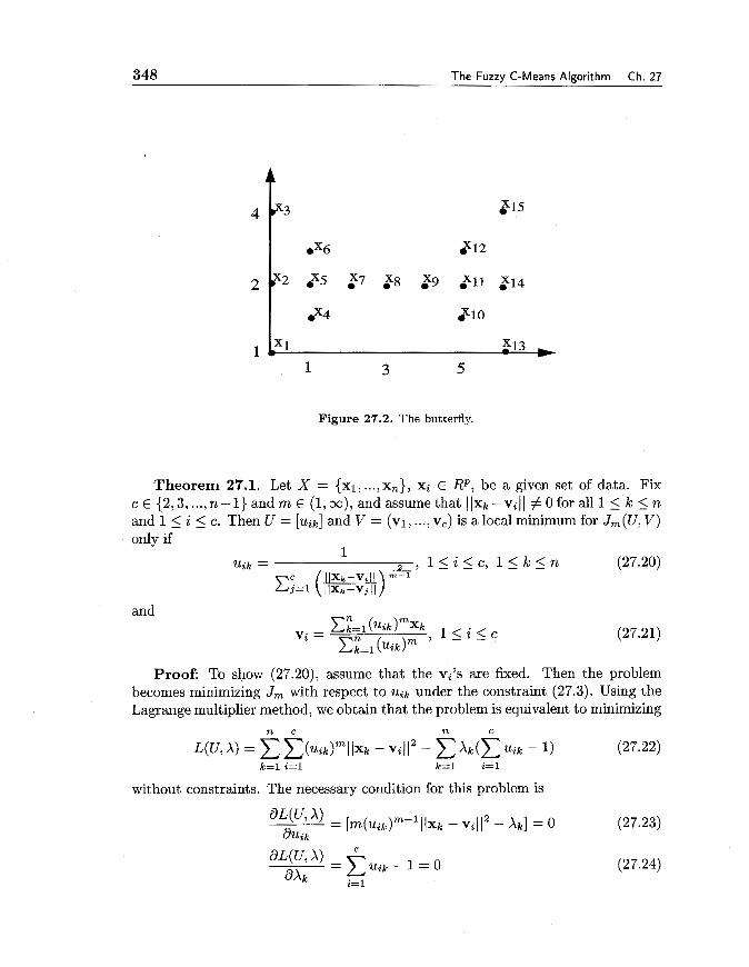
348 The Fuzzy C-Means Algorithm Ch. 27
Figure 27.2. The butterfly.
Theorem 27.1. Let X = { x l , ..., x,), xi E RP, be a given set of data. Fix c E {2,3, ..., n - 1 ) a n d m E ( l , ~ ) , andassumethat IIxk--viII #Oforall1 5 k < n and 1 5 i 5 c. Then U = [uik] and V = (vl , ..., v,) is a local minimum for Jm(U, V) only if
and
Proof: To show (27.20), assume that the vi 's are fixed. Then the problem becomes minimizing Jm with respect to uik under the constraint (27.3). Using the Lagrange multiplier method, we obtain that the problem is equivalent to minimizing
n c n c
L(U, A) = C C ( ~ i / c ) ~ l l * k - vi1I2 - C A.(C ~ i l - 1) (27.22) k=l i=l k=l i=l
without constraints. The necessary condition for this problem is
Sec. 27.3. Hard and Fuzzv c-Means Algorithms 349
From (27.23), we have
Substituting (27.25) into (27.24), we have
Substituting (27.26) into (27.25), we obtain (27.20).
To show (27.21), assume that uik's are fixed. Then this is an unconstraint minimization problem and the necessary condition is
from which we get (27.21).
The fuzzy c-means algorithm is based on the necessary condition (27.20) and (27.21).
Fuzzy c-Means Algorithm:
Step 1. For given data set X = {XI , ..., xn), xi E RP, fix c E {2,3, ..., n - I), m E (1, m), and initialize u(O) E M f c
Step 2. At iteration 1, I = 0,1 ,2 , ..., compute the c mean vectors
Step 3. Update u(~) = [ui?] to U(l+') = [u!rl)] using
Step 4. If IIU("l) - u ( ' ) I J < E , stop; otherwise, set 1 = 1 + 1 and go to Step 2.
We now apply the fuzzy c-means algorithm to the butterfly example.
Example 27.3. Let X = {x l , ..., xI5) be the butterfly data in Fig. 27.2. With c = 2 , m = 1 . 2 5 , ~ = 0.01, and
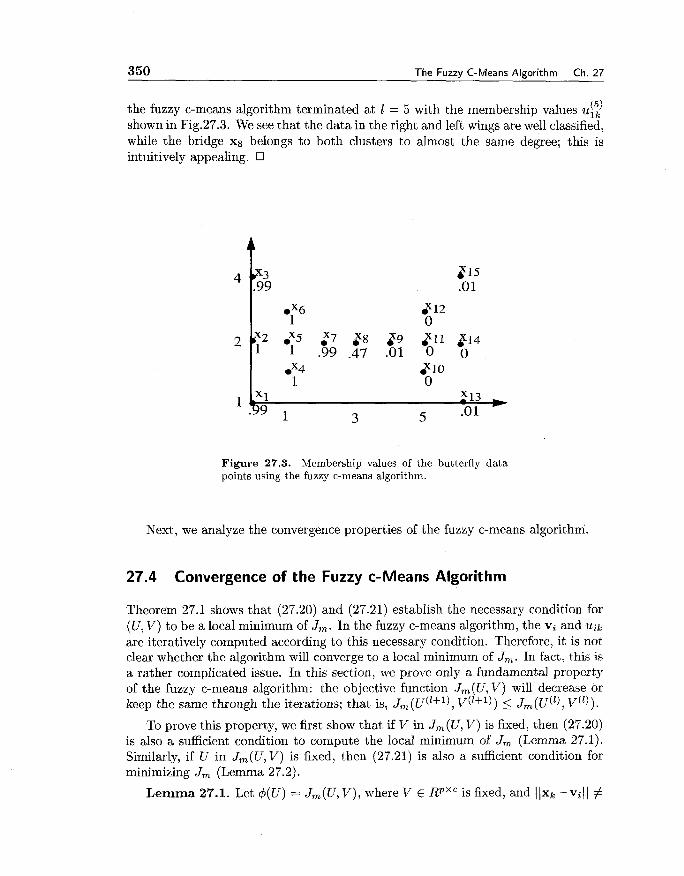
350 The Fuzzy C-Means Algorithm Ch. 27
( 5 ) the fuzzy c-means algorithm terminated at 1 = 5 with the membership values ulk shown in Fig.27.3. We see that the data in the right and left wings are well classified, while the bridge x* belongs to both clusters to almost the same degree; this is intuitively appealing.
Figure 27.3. Membership values of the butterfly data points using the fuzzy c-means algorithm.
Next, we analyze the convergence properties of the fuzzy c-means algorithni.
27.4 Convergence of the Fuzzy c-Means Algorithm
Theorem 27.1 shows that (27.20) and (27.21) establish the necessary condition for (U, V) to be a local minimum of J,. In the fuzzy c-means algorithm, the vi and uik are iteratively computed according to this necessary condition. Therefore, it is not clear whether the algorithm will converge to a local minimum of Jm. In fact, this is a rather complicated issue. In this section, we prove only a fundamental property of the fuzzy c-means algorithm: the objective function Jm(U, V) will decrease or keep the same through the iterations; that is, J, (u('+'), v('+')) < J, ( ~ ( ' 1 , ~ ( ' 1 ) .
To prove this property, we first show that if V in J,(U, V) is fixed, then (27.20) is also a sufficient condition to compute the local minimum of Jm (Lemma 27.1). Similarly, if U in J,(U, V) is fixed, then (27.21) is also a sufficient condition for minimizing Jm (Lemma 27.2).
Lemma 27.1. Let $(U) = J,(U, V), where V E RpXC is fixed, and I Ixk - vill #

Sec. 27.4. Convergence of the Fuzzy c-Means Algorithm 351
0 for all 1 5 k 5 n and 1 5 i < c. Then U = [uik] is a local minimum of 4(U) if and only if U is computed via (27.20).
Proof: The only if part was proven in Theorem 27.1. To show the sufficiency, we examine H(U) - the cn x cn Hessian of the Lagrangian of 4(U) evaluated at the U given by (27.20). From (27.23), we have
m(m - l ) ( ~ , t ) ~ - ~ 1 1 x t - v,1I2 if s = i , t = k 0 otherwise
(27.31) where u,t is computed from (27.20). Thus, H(U) = [hst,ik(U)] is a diagonal matrix. Since m > 1 and ((xi - v,(( # 0 for all 1 5 t 5 n and 1 < s 5 c, we have m(m - 1) ( ~ , t ) ~ - ~ I (xt - V, 1 l2 > 0. Therefore, the Hessian H (U) is positive definite and consequently (27.20) is also a sufficient condition for minimizing $(U).
Lemma- 27.2. Let $(V) = Jm(U,V), where U E Mf, is fixed, ((xk - v i ( ( # 0 for 1 < k 5 n and 1 5 i < c, and m > 1. Then V = [vi] is a local minimum of $(V) if and only if V is computed via (27.21).
Proof: The necessity was proven in Theorem 27.1. To show the sufficiency, we have from (27.27) that
C i = l 2 ( ~ ~ ~ ) ~ if j = i otherwise
Therefore, the Hessian is positive definite and consequently (27.21) is a sufficient condition for minimizing (V) .
From Lemmas 27.1 and 27.2, we can prove our main result: J,(u('+'), v('+')) < - J ~ ( u ( ' ) , ~ ( ' 1 ) .
Theorem 27.2. Let v,!" , u:?, I = 0,1,2, ..., be the sequence generated from the
fuzzy c-means algorithm (27.28) and (27.29). If m > 1 and (lxf) - vil)I( # 0 for all k = 1,2, ..., n, i = 1,2, ..., c, and 1 = 0,1,2, ..., then we have
Proof: Since v(') is computed from (27.28) fqr fixed U, we have from Lemma 27.2 that
J m (u(I+l), v(I+l)) < - J ~ ( U ( ' + ~ ) , ~ ( ' 1 ) (27.34)
Since u('+') is computed from (27.29) for fixed V, we have from Lemma 27.1 that
Combining (27.34) and (27.35), we obtain (27.33).

352 The Fuzzy C-Means Algorithm Ch. 27
Let R be the set
R = {(U*, V") E M f c x R p X C I Jm(U*, V*) 5 Jm(U, V*),VU E M f C ; Jm(U*,V*) < J,(U*, V), V # V*) (27.36)
Then it was proven in Bezdek, Hathaway, Sabin and Tucker [I9871 that the fuzzy c-means algorithm either terminates at a point in 0, or a subsequence exists that converges to a point in 0. For details, the readers are referred to Bezdek, Hathaway, Sabin, and Tucker [1987].
27.5 Summary and Further Readings
In this chapter we have demonstrated the following:
e The motivations of using fuzzy models for pattern recognition.
The definitions of hard and fuzzy c-partitions and the steps of the hard c- means algorithm.
The detailed steps of the fuzzy c-means algorithm and its theoretical justifi- cation.
The convergence properties of the fuzzy c-means algorithm.
The original book Bezdek [I9811 is still the best source to learn the fuzzy c- means algorithm. A number of important papers on the fuzzy c-means algorithm and other algorithms in fuzzy approaches to pattern recognition are collected in the edited book Bezdek and Pal [1992]. For classical methods for pattern recognition, see Duda and Hart [1973].
27.6 Exercises
Exercise 27.1. Show that the number of distinct ways to partition n elements into c nonempty subsets is given by (27.9).
Exercise 27.2. Let U E Adfc and
Show that:
(a) ( l lc ) < F(U) < 1 for any U E M f c .
(b) F(U) = 1 if and only if U is hard.

Sec. 27.6. Exercises 353
(c) F ( U ) = (l /c) if and only if uu = (l/c)Vi, k.
Exercise 27.3. Let x l , ..., x n be n d-dimensional samples and C be any non- singular d-by-d matrix. Show that the vector x that minimizes
is the sample mean A xi=, x k
Exercise 27.4. Verify that (27.16) is necessary to minimize JW (U, V) of (27.12) for fixed V.
Exercise 27.5. Prove that Jw(U, V) of (27.12) decreases monotonically as c increases.
Exerc i se 27.6. Repeat Example 27.3 with the initial partition
where (x)~,, is a 1 x r vector with all its elements equal to x.
Exercise 27.7. Apply the fuzzy c-means algorithm to the butterfly data with c = 3, m = 1.25, c = 0.01, and
Exercise 27.8. Develop a design method for fuzzy systems from input-output pairs based on the fuzzy c-means algorithm.

Chapter 28
Fuzzy Relation Equations
28.1 Introduction
Given fuzzy set A in the input space U and fuzzy relation Q in the input-output product space U x V, the compositional rule of inference (Chapter 6) gives a fuzzy set B in V as
P B ( Y ) = SUP(PA(X) * P Q ~ 2/11 (28.1) xEU
Let o denote the sup-star composition, then (28.1) can be rewritten as
If we view the fuzzy relation Q as a pure fuzzy system (see Chapter l ) , then (28.1) or (28.2) tells us how to compute the system's output B given its input A and the system itself Q. Sometimes, it is of interest to consider the following two problems:
Given the system Q and its output B , determine the corresponding input A. This is similar to the deconvolution or equalization problems in signal pro- cessing and communications, so we call this problem the "fuzzy deconvolution problem."
Given the system's input A and output B, determine the system Q. This is similar to the system identification problem in control, so we call this problem the "fuzzy identification problem."
Therefore, solving the fuzzy relation equation (28.2) means solving the above two problems. The objective of this chapter is to study how to obtain the solutions to the two problems.
28.2 Solving the Fuzzy Relation Equations
In this section, we first introduce a useful operator-the cp-operator, and study its properties. Then, we prove a few lemmas from which we obtain solutions to the

Sec. 28.2. Solving the Fuzzy Relation Equations 355
fuzzy identification and fuzzy deconvolution problems.
Definition 28.1. The cp-operator is a two-place operator cp : [O, 11 x [ O , l ] -+ [O, 11 defined by
acpb = sup[c E [O,l]la*c < b] (28.3)
where * denotes t-norm operator.
Clearly, for &fferent t-norms * we have different cp-operators. For the * specified as minimum, the cp-operator becomes the so-called a-operator:
1 i f a s b aab = sup[c E [O,l]lmin(a, c) 5 b] = b i f a > b
We now show some useful properties of the cp-operator.
Lemma 28.1. Let the cp-operator be defined by (28.3). Then the following inequalities are true:
acpmax(b, c) > max(acpb, acpc) (28.5)
a * (acpb) 5 b (28.6)
acp(a * b ) >_ b (28.7)
where a, b, c E [0, 11 (usually, a, b, c are membership functions).
Proof: From (28.3) it is clear that acpb is a nondecreasing function of the second argument b, that is, apbl > apb2 if bl 2 b2. Hence, acpmax(b,c) > acpb and acpmax(b, c) 2 acpc; this gives (28.5). (28.6) is a direct conclusion of the definition (28.3). Finally, from acp(a * b) = sup[c E [O,l]la * c < a * b] and the nondecreasing property of t-norm, we obtain (28.7).
Now consider the "fuzzy identification problem," that is, solving the fuzzy rela- tion equation (28.2) for Q given A and B. We will show that a particular solution is Q = AcpB. To prove this result, we need the following two lemmas.
Lemma 28.2. Let A be a fuzzy set in U and Q be a fuzzy relation in U x V. Then,
& c 4 4 . 4 Q) (28.8)
where Acp(AoQ) is a fuzzy relation in U xV with membership function pA(~)cpPAoQ(~)
Proof: Since acpb is a nondecreasing function of b, we have
Using (28.7) we get P A ~ ( A ~ Q ) (x, Y) 2 P Q ~ , Y)
which gives (28.8). Cl

356 Fuzzy Relation Equations Ch. 28
Lemma 28.3. Let A and B be fuzzy sets in U and V, respectively. Then,
where ApB is a fuzzy relation in U x V with membership function pA(x)ppB(y).
Proof: From (28.6) we have
which is equivalent to (28.11).
We are now ready to determine a solution to the "fuzzy identification problem."
Theorem 28.1. Let Q be the set of all solutions Q of the fuzzy relation equation (28.2) given A and B. If & is non-empty, then the largest element of Q (in the sense of set-theoretic inclusion) is given by
Proof: Let Q be an arbitrary element of Q, then B = A o Q and from Lemma 28.2 we have Q C ApB = Q. Since t-norms are nondecreasing functions, we have B = A o Q A o Q. But from Lemma 28.3 we have A o Q = A o (ApB) B, hence B = A o Q, which means Q is an element of &. Since Q c Q and Q is an arbitrary element of Q , we conclude that Q is the largest element of &.
Next, we consider the "fuzzy deconvolution problem," that is, solving the fuzzy relation equation (28.2) for A given B and Q. Again, we first prove two lemmas from which we determine a possible solution.
Lemma 28.4. Let B be a fuzzy set in V and Q be a fuzzy relation in U x V. Then,
(&@) 0 & C B (28.14)
where the composition (QpB) o Q is a fuzzy set in V with membership function SUP,EU[I-LQ~B(X, Y) * PQ(X, ~ 1 1 .
Proof: From (28.6) we get
which gives (28.14).

Sec. 28.2. Solving the Fuzzy Relation Equations 357
Lemma 28.5. For fuzzy set A in U and fuzzy relation Q in U x V, the following is true:
A c Qp(A Q)
where Qcp(AoQ) is a fuzzy set in U with membership function supyEV[pQ (x, y)ppAoQ (st)].
Proof: Using (28.7) and the fact that apb is a nondecreasing function of b, we have
>_ SUP [PA (XI] = PA (x) YEV
which gives (28.16).
We are now ready to give a compact formula of the solution to the "fuzzy deconvolution problem."
Theorem 28.2. Let d be the set of all solutions A of the fuzzy relation equation (28.2) given B and Q. If A is non-empty, then the greatest element of A is given by
A = Q ~ B (28.18)
where Q p B is a fuzzy set in U with membership function supyEv[pQ(x, y)ppB(y)].
Proof: Let A be an arbitrary element of A, so B = A o Q and from Lemma 28.5 we have A C Qp(Ao Q) = Q p B = A, which implies B = Ao Q A o Q. From Lemma 28.4 we have A o Q = (QpB) o Q 2 B, hence A o Q = B, which means that A is an element of A. Since A is an arbitrary element in A and we have shown A c A, A is the largest element of A.
A fundamental assumption in Theorems 28.1 and 28.2 is that the solutions to the problems exist. In many cases, however, an exact solution may not exist. Therefore, Q = AcpB and A = Q p B may not be the solutions; see the following example.
Example 28.1. Let U = { x ~ , x z ) , V = {yl, y2), and
Let the cp-operator be the a-operator (28.4), then
Q = A@ = ~ / ( x I , Y ~ ) + ~/ (x I ,Yz) + 1/(xz,y1) + l / ( x 2 , ~ 2 ) (28.22)
Using min for the t-norm in the sup-star composition, we have
A 0 Q = 0.4/y1 + 0.41~2 # B (28.23)

358 Fuzzv Relation Eauations Ch. 28
Hence, Q = ApB is not a solution to the problem. Similarly, using a-operator for cp and min for the t-norm, we have
and
17
Under what conditions do the solutions to the "fuzzy identification and decon- volution problems" exist? We answer this question in the next section.
28.3 Solvability Indices of the Fuzzy Relation Equations
Since B and A o Q are fuzzy sets in V, whether the fuzzy relation equation (28.2) is solvable is equivalent to whether the two fuzzy sets B and A o Q are equal. Therefore, we must first study how to measure the equality of two fuzzy sets.
28.3.1 Equality Indices of Two Fuzzy Sets
Let C and D be two fuzzy sets in U . Then, a natural measurement of the difference between C and D is
For p = 1 one has the Hamming distance, and p = 2 yields the Euclidean distance. The equality index of C and D is defined as
Clearly, eqt(C, D) = 1 if and only if C = D, therefore eqp(C, D) is qualified as an equality index. Since the computation of d,(C, D) involves the complicated integration, it is helpful to explore other measures of equality of two fuzzy sets.
Another approach to the comparison of fuzzy sets is to use more set-theoretically oriented tools. First, from the definition of the cp-operator (28.3) and the bound- ary condition of t-norm (see Chapter 3) we have that C D if and only if infZEu[pc(x)cpp~(x)] = 1. Since C = D is equivalent to C D and D C C, we can define the equality index of C and D as
Clearly, eqt(C, D) = 1 if and only if C = D, therefore eqt(C, D) is qualified as an equality index. Using the facts that acpb = 1 if and only if a 5 b and that the second

Sec. 28.3. Solvability Indices o f the Fuzzy Relation Equations 359
infxEu in (28.28) can be moved in the front (due to the continuity of t-norm), we can rewrite the equality index as
where V denotes maximum, and A denotes minimum.
We are now ready to define the solvability indices for the fuzzy relation equation.
28.3.2 The Solvability Indices
Using the equality index of two fuzzy sets, it is natural to define the solvability index of the fuzzy relation equation (28.2) as
However, since either A or Q is unknown, J cannot be computed. From Theorems 28.1 and 28.2 we know that a possible solution to the "fuzzy identification (decon- volution) problem" is Q = ApB (a = QpB), a way to define the solvability indices is to replace the Q in (28.30) by Q and A by A. Specifically, we have the following definition.
Definition 28.2. The solvability index of the yuzzy identification problem" is defined as
EI = eqt [A 0 (A@), B] (28.31)
and the solvability index of the (yuzxy deconvolution problem" is defined as
Clearly, G = 1 (ED = 1) not only means that the "fuzzy identification (decon- volution) problem" is solvable but also implies that Q = ApB (A = QpB) is a solution. Since we use these special solutions in defining and to, one may won- der whether 51 # 1 ([D # 1) implies that the "fuzzy identification (deconvolution) problem" is not solvable because we may have Q' (A') other than ApB (QpB) such that eqt (AO Q', B) = 1 (eqt (2 0 Q, B) = 1). Fortunately, this Q' (a') does not exist, because from Theorems 28.1 and 28.2 we know that if Q = ApB (A = QpB) is not a solution to the "fuzzy identification (deconvolution) problem," then no other solution exists. Therefore, 51 = 1 ( 5 ~ = 1) if and only if the "fuzzy identification (deconvolution) problem" is solvable.
Our next task is to simplify JI and ( D to make them easy to compute. First, we need the following lemma.
Lemma 28.6. For a , b E [0, 11, it holds that
a * (acpb) = min(a, b)
bcp(a * (apb)) = bpa

360 Fuzzy Relation Eauations Ch. 28
Proof: If a < b, then apb = 1 and a * (acpb) = a = min(a, b). If a > b, then from the definition of p-operator we have a * (apb) = a * sup[c E [O, llla * c 5 b] = sup[a * c(a * c 5 b] = b = min(a, b); this proves (28.33). For (28.34), we have from (28.33) that bq(a* (apb)) = bp[min(a, b)] = bpa, which is obvious for a < b, but in the b < a case we have bpb = 1 = bpa.
The following theorem shows that 51 and tD are simple functions of the heights of A, B and Q.
Theorem 28.3. Let hgh(A), hgh(B) and hgh(Q) be the heights of A, B and Q, respectively (recall that hgh(A) = ~ u p , , ~ p ~ ( x ) ) . Then,
Proof: Since A o (AcpB) C B (Lemma 28.3), we have from (28.31) and (28.29) that
From the monotonicity of p in the second argument, we get
Using (28.34) we have
Since p is a monotonic nonincreasing function of the first argument, the infyEv in (28.29) is achieved when ~ ~ ( y ) equals its maximum value. Hence,
The proof of (28.36) is left as an exercise.
We can now go back to Example 28.1 and see why an exact solution does not exist. For the A, B and Q in (28.19)-(28.21), we have hgh(A) = 0.4, hgh(B) = 0.5 and hgh(Q) = 0.3, therefore cI = 0.5p0.4 # 1 and E D = 0.5p0.3 # 1. If an exact solution does not exist, what we can do is to determine approximate solutions; this is the topic of the next section.

Sec. 28.4. A ~ ~ r o x i m a t e Solution-A Neural Network Amroach 361
28.4 Approximate Solution-A Neural Network Approach
From Theorem 28.3 and the definition of the cp-operator we see that if the height of B is larger than the height of A or Q, exact solutions do not exist. In these cases, a natural way is to determine A or Q such that
is minimized; this gives the least-squares solution. Here we consider only the "fuzzy deconvolution problem;" the "fuzzy identification problem" can be solved in a simi- lar fashion. To make the minimization of (28.41) trackable, we do the following two things: (i) parameterize p ~ ( x ) as the Gaussian function (we also can use triangular or trapezoidal function)
where Z and a are free parameters, and (ii) make samples xi and yj (i = 1,2, ..., N, j = 1,2, ..., M) over the domains U and V, respectively, and approximate (28.41) by
Therefore, the problem becomes determining the parameters Z and a, such that (28.43) is minimized.
We now develop a neural network approach to this problem. First, we represent pA (x)pQ (x, y) as the network shown in Fig. 28.1, where a = exp[- 4 (v)2], b = pQ(x, y), and z = ab. For fixed y = yj, we compute zl, z2, ..., z~ for x = xl, 2 2 , ..., xw, and determine Zi* = max[z~ , ..., z ~ ] . Clearly, zi* equals the m a x ~ < ~ < ~ [ p ~ ( x i ) p ~ (xi, yj)] in (28.43). We then adjust the parameters 2 and o to minimizethe squared error
using a gradient descent algorithm. The details of this method is given as follows.
A Neural Network Approach to the "Fuzzy Deconvolution Problem"
Step 1: Make samples x, (i = 1,2 , ..., N) over the domain U and samples y, \ (j = 1,2, ..., M ) over the domain V. If U and V are bounded, we usually make the samples uniformly distributed over U and V. Determine initial guesses Z(0) of Z and a(0) of 0. Sometimes, human experts can provide these initial guesses. If not, choose Z(0) randomly in U and choose a to be a reasonable positive number, for example, a = 1. Initialize j = 1.

362 Fuzzy Relation Equations Ch. 28
Figure 28.1. Network representation of p~(x)p&(x, y).
Step 2: Fix y = y j in the network of Fig. 28.1, and for x = X I , 2 2 , ..., X N com- pute forward along the network to determine the corresponding z l , zz, ..., z ~ . Find i* such that zi* = max[z l , z2, .. ., zN] .
Step 3: Update the parameters % and a using the gradient descent algorithm:
where
ei is given by (28.44), and k = 0,1,2, ....

Sec. 28.4. A ~ ~ r o x i m a t e Solution-A Neural Network Approach 363
Step 4: Go to Step 2 with y = yj+l, and repeat for y = yl, y2, ..., y ~ , y1, ..., until the differences I5(k + 1) - ~ ( k ) 1 and lo(k + 1) - a(k) 1 are smaller than a small threshold for a number of k's greater than M.
The training algorithm (28.45) and (28.46) are obtained by using the chain rule:
3 = 2e .% = -2ej && = -2e .b* Bh = -aejb a ae2
az 3 az 3 az * * ; similar for . It can be proven that the above training algorithm guarantees that the total matching error x:, e: will decrease after every M steps of training. Because it is required that a > 0, in the implementation we need to choose a small constant E > 0 such that if o(k + 1) > E then keep a(k + 1) as computed by (28.46), and if o(k + 1) 5 .c then set a(k + 1) = E . In this way we can guarantee a(k) 2 E for all k.
We now simulate the algorithm for an example.
Example 28.2. Consider a fuzzy relation that is characterized by the two fuzzy IF-THEN rules:
RU('): I F x i s s m a l l , T H E N y i s n e a r l , (28.49)
R U ( ~ ) : IF x i s large, THEN y i s near 0, (28.50)
where "small," "large," "near 1," and "near 0" are fuzzy sets with membershit 1 1 functions: ,Usmall (x) l+elo(.-l) 7 plarge (2) = 1+e10(-2+3) 1 h e a r 1 (Y) = e-lO(y-l)
and pnearo(y) = e-log2, respectively. Using Mamdani's product implication, the R U ( ~ ) (i=1,2) are fuzzy relations in U x V with membership functions
The final fuzzy relation Q is
e-10(y-1)2 e-10y2
= max 1 + e l O ( ~ - l ) ' 1 + e10(-~+3) I Now, for simplicity, we assume that o = 1 in (28.42), and our task is to determine
5 for different pB(y)'s. We consider three cases of p ~ ( y ) : (i) pB(y) = e-10(y-0.5)2 (that is, y is near 0.5), (ii) ,uB(y) = ~ - ' O ( Y - ' ) ~ (that is, y is near I) , and (iii) p~ (y) = e-1°y2 (that is, y is near 0). We choose the domains U = [O, 41 and V = [O, 11. We uniformly sample U and V with N = 17 and M = 9 points, respectively, that is, (XI, x2,x3, ..., 217) = (0,0.25,0.5, ..., 4), and (yl, yz, ys, ..., y9) = (0,0.125,0.25, ..., 1). Figs.28.2-28.4 show the convergence procedures of Z(k) for different initial conditions for the three PB (y) cases (i)-(iii), respectively, where the horizontal axis represents the k in the training algorithm, and the vertical axis represents the %(k). From Figs. 28.2-28.4 we see that the training procedure converged in about 10 steps for all the three cases.

364 Fuzzy Relation Equations Ch. 28
Figure 28.2. Convergence procedure of Z ( k ) for p y ( y ) = e-lo(y-055)2.
Figure 28.3. Convergence procedure of ~ ( k ) for pY ( y ) = e - l o ( ~ - l ) 2 .

Sec. 28.5. Summarv and Further Readinas 365
Figure 28.4. Convergence procedure of Z ( k ) for py(y ) = e - 1 0 ~ 2 ,
From Fig. 28.2 we see that in this case all the 5(k) 's for different initial ~ ( 0 ) ' s converged to the same value near 2. This is consistent with our intuition because from (28.49) and (28.50) we expect that if y is near 0.5, that is, in the middle of 0 and 1, then x should be in the middle of "small" and "large" which, by observing the membership functions p,,,n and p~ll,,,,, is somewhere around 2. Figures 28.3 and 28.4 show that for " y is near 1" and " y is near O", the 5 ( k ) converged to a region of values for different initial conditions, not to a single point. This also is intuitively appealing because from (28.49) we see that if y is near 1, then x should be small, which in Fig. 28.3 means somewhere between -0.3 and 0.8. Similarly, from (28.50) we see that if y is near 0 , then x should be large, which in Fig. 28.4 means somewhere between 3.2 and 4.3. In summary, all the solutions in the three cases are consistent with our intuition.
I
28.5 Summary and Further Readings
In this chapter we have demonstrated the following:
The definition of "fuzzy deconvolution and fuzzy identification problems."
How to obtain the particular solutions to the problems.
The definition and computation of the solvability indices.

366 Fuzzy Relation Equations Ch. 28
How to transform the problems of solving the fuzzy relation equations into a neural network framework and how to develop a training algorithm for computing the approximate solutions.
A special book on fuzzy relation equations is Nola, Sessa, Pedrycz, and Sanchez [1989]. The book Pedrycz [I9931 also covered the fuzzy relation equations exten- sively. A good tutorial paper for fuzzy relation equations is Pedrycz [1991]. The neural network approach in this chapter was taken from Wang [1993b].
28.6 Exercises
Exercise 28.1. Solve the following "fuzzy deconvolution problems" for the max-min composition.
.9 .8 .7 (a) A o [ 8 9 8 ] = 1.6 5 41 (28.54)
.7 .8 .9
( b ) A 0 1 '4 " O 1 = [.5 .5 4 .2] .2 .4 .5 .6
Exercise 28.2. Solve the following "fuzzy identification problems" for the max- min composition.
(a) [I .3 .5] o Q = [.6 .5 .4]
( b ) [.I .3 .5 .7] o Q = [.6 .5 .4 .3] (28.59)
Exercise 28.3. Prove (28.36) in Theorem 28.3.

Sec. 28.6. Exercises 367
Exercise 28.4. Let P, Q and R be fuzzy relations in U x V, V x W and U x W, respectively, and F(U x V) be the set of all fuzzy relations in U x V. Define the solvability index of the fuzzy relation equation P o Q = R as
6 = sup eq t (PoQ,R) P E F ( U X V )
Show that
Exercise 28.5. Develop a neural network approach for solving the "fuzzy iden- tification problem."

Chapter 29
Fuzzy Arithmetic
29.1 Fuzzy Numbers and the Decomposition Theorem
In the fuzzy IF-THEN rules, the atomic fuzzy proposition, xi is A:, is often an imprecise characterization of numbers in the real line R, for example, "close to 5," "approximately 7," etc. Since fuzzy sets defined in R appear quite often in many applications, they deserve an in-depth study. Roughly speaking, a fuzzy number is a fuzzy set in R; but in order to perform meaningful arithmetric operations, we add some constraints. Specifically, we have the following definition.
Definition 29.1. Let A be a fuzzy set in R. A is called a fuzzy number if: (i) A is normal, (ii) A is convex, (iii) A has a bounded support, and (iv) all a-cuts of A are closed intervals of R.
We require a fuzzy number to be normal because our conception of real numbers close to r is fully satisfied by r itself, hence we should have p~ (r) = 1. The convexity and boundedness conditions allow us to define meaningful arithmetric operations for fuzzy numbers.
Two special classes of fuzzy numbers often are used in practice; they are trian- gular and trapezoidal fuzzy numbers. A triangular fuzzy number A is a fuzzy set in R with the triangular membership function:
Similarly, if a fuzzy set A in R has the trapezoidal membership function:
it is called trapezoidal fuzzy number. It is easy to check that the triangular and trapezoidal fuzzy numbers satisfy the four conditions in Definition 29.1.

Sec. 29.2. Addition and Subtraction of Fuzzy Numbers 369
A useful approach to study the arithmetic operations of fuzzy numbers is to use the a-cuts of fuzzy numbers. Recall that the a-cut of a fuzzy set A in R is defined as
A, = {x E R)PA(x) > a) (29.3)
Now we show that a fuzzy set can be uniquely determined by its a-cuts. To make precise representation, we define fuzzy set A", in R with the membership function
where IA,(x) is the indicator function of the (crisp) set A,, that is, IAa(x) = 1 if x E A, and IA, (x) = 0 if x E R - A,. The following theorem, known as the Decomposition Theorem, states that the fuzzy set A equals the union of the fuzzy sets A", for all a E [0, 11.
Theorem 29.1. (Decomposition Theorem) Let A and & be fuzzy sets in R with A, defined by (29.4). Then,
where U denotes the standard fuzzy union (that is, sup over a E [O,l]).
Proof: Let x be an arbitrary point in R and a = PA($). Then.,
For each a E (a, 11, we have pA(x) = a < a and thus x # A, which implies p~ (x) = 0. If a E [0, a], then PA(X) = a 2 a so that x E A, and from (29.4) we have (x) = a. Hence,
- (x) = SUP a = a = p ~ ( x ) PUae[o,l] A,
(29.7) ff€[o,al
Since x is arbitrary, (29.7) implies (29.5).
From Theorem 29.1 we see that if we can determine the a-cuts of a fuzzy set for all a E [0, 11, we can specify the fuzzy set itself. Therefore, determining a fuzzy set is equivalent .to determining its a-cuts for all a E [O,l]. In the next two sections, we will use the a-cuts to define the arithmetic operations of fuzzy numbers.
29.2 Addition and Subtraction of Fuzzy Numbers
29.2.1 The a-Cut Method
Let A and B be two fuzzy numbers and A, = [a;, a:], B, = [b;, b i ] be their a-cuts. Then, the addition of A and B, A + B, is a fuzzy number with its a-cuts

370 Fuzzy Arithmetic Ch. 29
defined by (A + B) , = [a; + b;, a: + b:]
for every a E [0, 11. Since a fuzzy set is completely determined by its a-cuts (The- orem 29.1), the fuzzy number A + B is well-defined by its a-cuts (29.8).
Similarly, the subtraction of A and B , A - B, is a fuzzy number with its a-cuts defined by
(A - B), = [min(a, - b;, a: - b:), max(a; - b;, a: - b:)]
for every a E [0, I].
Example 29.1. Compute the addition and subtraction of the triangular fuzzy numbers A and B whose membership functions are
For a given a E [O,l], the a-cuts of A and B are
Hence, ( A + B), = [3a-2 ,4-3a]
Since 3 a - 2 and 4 - 3 a are linear functions of a , A + B is also a triangular fuzzy number. By setting a = 0 and a = 1 in (29.13), we obtain
which is plotted in Fig. 29.1. Similarly, we have
(A - B), = [a - 2, -a] (29.15)
and PA-~($1 = PA-B(X; -2, -1,O)
which is shown in Fig. 29.1.
Another way to compute the addition and subtraction of fuzzy numbers is to use the extension principle.
29.2.2 The Extension Principle Method
Using the extension principle (Chapter 4), we can define the addition of fuzzy numbers A and B as
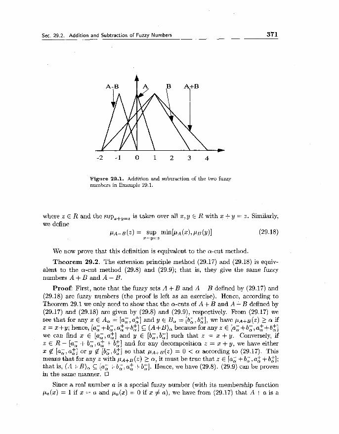
Sec. 29.2. Addition and Subtraction of Fuzzy Numbers 371
Figure 29.1. Addition and subtraction of the two fuzzy numbers in Example 29.1.
where z E R and the sup,+,,, is taken over all x, y E R with x + y = z . Similarly, we define
P A - ~ ( 2 ) = SUP m i n [ ~ ~ ( x ) , PB (Y)] (29.18) x-,=z
We now prove that this definition is equivalent to the a-cut method.
Theorem 29.2. The extension principle method (29.17) and (29.18) is equiv- alent to the a-cut method (29.8) and (29.9); that is, they give the same fuzzy numbers A + B and A - B.
Proof: First, note that the fuzzy sets A + B and A - B defined by (29.17) and (29.18) are fuzzy numbers (the proof is left as an exercise). Hence, according to Theorem 29.1 we only need to show that the a-cuts of A + B and A - B defined by (29.17) and (29.18) are given by (29.8) and (29.9), respectively. From (29.17) we see that for any x E A, = [a;, a:] and y E B, = [b;, b:], we have PA+B (z) 2 a if z = x + y; hence, [a; + b;, a: + b:] C_ (A+ B), because for any z E [a; + b;, a: + b:] we can find x E [a;, a:] and y E [b;, b i ] such that z = x + y. Conversely, if z E R - [a; -t b;, a: + b:] and for any decomposition z = x + y, we have either x $! [a;,a$] or y $Z [b;, b$] so that PA+B(Z) = 0 < a according to (29.17). This means that for any z with PA+B(Z) 2 a, it must be true that z E [a; + b;, a; + b:]; that is, (A + B), 5 [a, + b;, a2 + b:]. Hence, we have (29.8). (29.9) can be proven in the same manner.
Since a real number a is a special fuzzy number (with its membership function ~ a ( x ) = 1 if x = a and p,(x) = 0 if z # a) , we have from (29.17) that A + a is a

372 Fuzzy Arithmetic Ch. 29
fuzzy number with membership function
P A + ~ ( z ) = PA(Z - a) (29.19)
That is, P ~ + ~ ( Z ) is obtained by shifting , u ~ ( z ) a distance of a. Similarly, A - a is a fuzzy number with membership function
PA-, (2) = PA (2 + a) (29.20)
Viewing 0 as a special fuzzy number, we have from (29.18) that
Finally, we consider an example of computing the addition and subtraction of two fuzzy sets defined over a finite number of points.
Example 29.2. Compute the addition and subtraction of the fuzzy sets:
Using (29.17) and (29.18), we have
29.3 Multiplication and Division of Fuzzy Numbers
29.3.1 The a-Cut Method
In classical interval analysis, the multiplication of intervals [a, b] and [c, d] is defined as
[a, b] . [c, d] = [min(ac, ad, bc, bd), max(ac, ad, be, bd)] (29.26)
If 0 $ [c, d], then the division of [a, b] and [c, dl is defined as
We now define the multiplication and division of fuzzy numbers using their a-cuts and (29.26)-(29.27).
Let A and B be fuzzy numbers and A, = [a;, a;] and B, = [b;, b;] be their a-cuts. Then, the multzpkication of A and B, A . B, is a fuzzy number with its a-cuts defined by
(A . B), = [min(a; b; , a; b:, a: b;, a: b:), max(a; b; , a; b:, a: b; , a: b:)] (29.28)

Sec. 29.3. Multiplication and Division of Fuzzy Numbers 373
for every a E [O,l]. If 0 6 [b;, b:] for all a E [0, 11, then the division of A and B , A/B, is a fuzzy number with its a-cuts defined by
(AIB), = [min(a;/b;, a,/b:, a:/b;, a:/b:), max(a,/b;, a,/b;,a:/b;, a;/b:)] (29.29)
for every a E [0, 11.
Example 29.3. Consider the fuzzy number A in Example 29.1 and B defined by
CLB(X) = PB (2; 0.5,1,3) (29.30)
We now compute A . B and A/B. First, note that the a-cuts A, = [a;, a:] = [a - 1 , l - a] and B, = [b;, b:] = [(a + 1)/2,3 - 2a]. Hence,
max(a,b,,a,b:,a:b,,a$b:) = sib: = 2a2 - 5 a + 3 (29.32)
and (A. B), = [-2a2 + 5a - 3, 2a2 - 5a + 31 (29.33)
From (28.33) we have
which is illustrated in Fig. 29.2. Similarly, we have
and
(A/% = [(a - 1)/(3 - 2a), 2(1- a ) / ( l + a)] (29.37)
From (29.37) we have
(32+1) / (22+1) for x < O ' A / ~ ( ~ ) = { (2-5)/(2+1) for X t O
which is plotted in Fig. 29.2.
29.3.2 The Extension Principle Method
Similar to addition and subtraction of fuzzy numbers, we can use the extension principle to define A . B and A/B. Specifically, the fuzzy numbers A - B and A/B are defined by
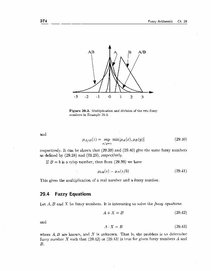
374 Fuzzv Arithmetic Ch. 29
Figure 29.2. Multiplication and division of the two fuzzy numbers in Example 29.3.
and
respectively. It can be shown that (29.39) and (29.40) give the same fuzzy numbers as defined by (29.28) and (29.29), respectively.
If B = b is a crisp number, then from (29.39) we have
This gives the multiplication of a real number and a fuzzy number.
29.4 Fuzzy Equations
Let A, B and X be fuzzy numbers. It is interesting to solve the fuzzy equations:
and A . X = B
where A, B are known, and X is unknown. That is, the problem is to determine fuzzy number X such that (29.42) or (29.43) is true for given fuzzy numbers A and B.

Sec. 29.4. Fuzzy Equations 375
We first study how to solve (29.42). Let A, = [a;, a:], B, = [b;, b:] and X, = [x;, 221. According to the Decomposition Theorem, (29.42) is true if and only if
[a;, 41 + [ x i , x:] = [b, , b:l (29.44)
for all a E (0, 11. Hence, a potential solution is given by
X , = [xi, ~ $ 1 = [ b i - a;, b: - a:] (29.45)
In order for the X, in (29.45) to be qualified as a-cuts, the following two conditions must be satisfied:
(i) b; - a; < b: - a 2 for every a E (0, 11
+ - + (ii) If a I p, then b; - a; 5 b j - I b$ - a$ 5 ba
Condition (i) guarantees that [b; - a;, b 2 - a:] is an interval, and condition (ii) ensures that [b; - a;, b; - a:] are nested intervals so that they are qualified as a-cuts of a fuzzy number. Therefore, if conditons (i) and (ii) are satisfied, then using the Decomposition Theorem we obtain the solution as
where X, are fuzzy sets defined by
Example 29.4. Let A and B be the triangular fuzzy numbers in Example 29.1. Then, from (29.12) we have a; = a - 1, a 2 = 1 - a , b; = 212 - 1 and b; = 3 - 2a. Hence, b; - a; = a and b 2 - a: = 2 - a. Since a 5 2 - a for a E (O,1] and a 5 /3 < 2 - p 5 2 - a if a 5 /3 5 1, conditions (i) and (ii) are satisfied. Therefore,
from which we obtain the solution X as the triangular fuzzy number
Next, we study the fuzzy equation (29.43). For simplicity, assume that A and B are fuzzy numbers in R+. Then (29.43) is equivalent to
for all a E (0, 11. If the following two conditions are satisfied:
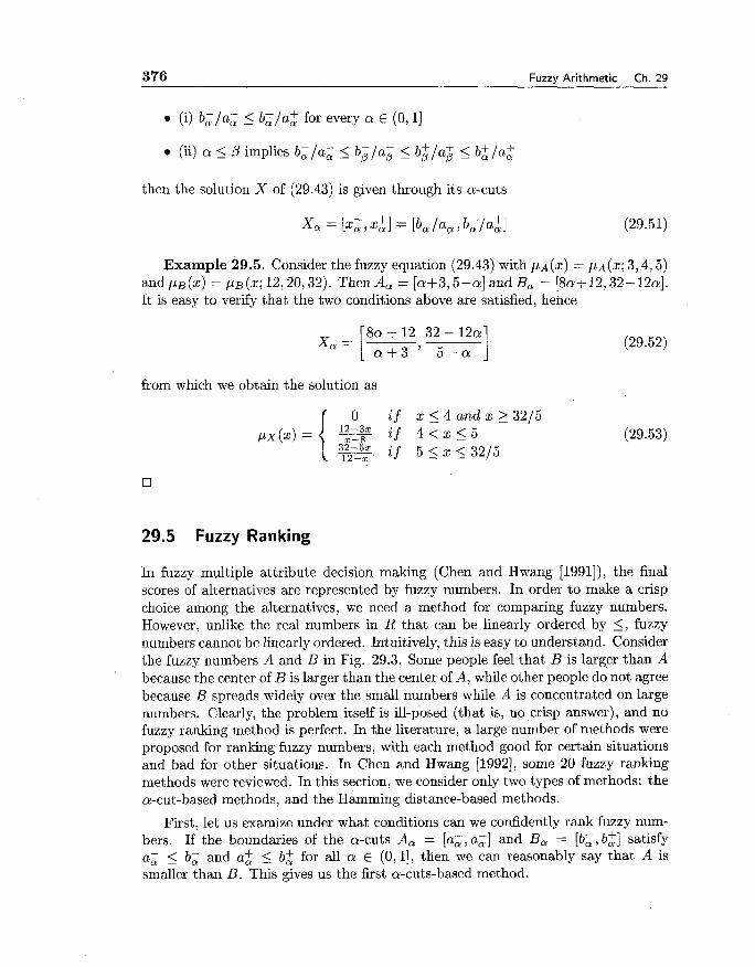
376 Fuzzy Arithmetic Ch. 29
m (i) b, /a; I b$/a; for every a E (O,l]
(ii) a < p implies b;/a; < bplap I b$/a$ I b:/a:
then the solution X of (29.43) is given through its a-cuts
+ + xo: = [ x i , 321 = [bJa;, b, la,]
Example 29.5. Consider the fuzzy equation (29.43) with pA (x) = pA (x; 3,4,5) and p ~ ( x ) = p ~ ( z ; 12,20,32). Then A, = [a+3,5-a] and B, = [8a+12,32-12aI. It is easy to verify that the two conditions above are satisfied, hence
from which we obtain the solution as
29.5 Fuzzy Ranking
In fuzzy multiple attribute decision making (Chen and Hwang [1991]), the final scores of alternatives are represented by fuzzy numbers. In order to make a crisp choice among the alternatives, we need a method for comparing fuzzy numbers. However, unlike the real numbers in R that can be linearly ordered by <, fuzzy numbers cannot be linearly ordered. Intuitively, this is easy to understand. Consider the fuzzy numbers A and B in Fig. 29.3. Some people feel that B is larger than A because the center of B is larger than the center of A, while other people do not agree because B spreads widely over the small numbers while A is concentrated on large numbers. Clearly, the problem itself is ill-posed (that is, no crisp answer), and no fuzzy ranking method is perfect. In the literature, a large number of methods were proposed for ranking fuzzy numbers, with each method good for certain situations and bad for other situations. In Chen and Hwang [1992], some 20 fuzzy ranking methods were reviewed. In this section, we consider only two types of methods: the a-cut-based methods, and the Hamming distance-based methods.
First, let us examize under what conditions can we confidently rank fuzzy num- bers. If the boundaries of the a-cuts A, = [a;, a;] and B, = [b;, b$] satisfy a; 5 b; and a$ < b; for all a E (0,1], then we can reasonably say that A is smaller than B. This gives us the first a-cuts-based method.

Sec. 29.5. Fuzzv Rankine: 377
Figure 29.3. Ranking fuzzy numbers is an ill-posed prob- lem.
a-cuts-based method 1: Let A and B be fuzzy numbers with a-cuts A, = [a;, a z ] and B, = [b;, bk] . We say A is smaller than B, denoted by A 5 B, if a; < b; and a: < b i for all a E (0, 11.
The advantage of this method is that the conclusion is less controversial. Its disadvantage is that it applies only to some obvious situations. For example, the A and B in Fig. 29.3 cannot be compared according this method, because b; 5 a; for small a but b; > a; for large a . Hence, a weaker ranking method was proposed, as follows:
a-cuts-based method 2: We say A < B if a 2 < b: for all a! E (c, 11, where c is a constant that is usually larger than 0.5.
Clearly, this method emphasizes the numbers with large membership values. According to this method, we have A 5 B for the A and B in Fig. 29.3.
Next, we consider the Hamming distance-based methods. The basic idea is to find a fuzzy number C such that A 5 C and B 5 C according to the (quite reasonable but restrictive) a-cuts-based method 1. Then, if the Hamming distance between C and A is larger than the Hamming distance between C and B, we conclude that A 5 B. Clearly, the choice of C is not unique. Here we choose the C to be the fuzzy number MAX(A, B) which is defined by

3 78 Fuzzy Arithmetic Ch. 29
Note that MAX(A, B) is different from the fuzzy set with membership function max(,uA,pB). It is easy to show that A < MAX(A,B) and B < MAX(A, B) according to the a-cuts-based method 1. Let the Hamming distance dl (C, D) be defined as in (28.26) with p = 1, then we have the following fuzzy ranking method:
Hamming distance-based method: We say A 5 B if dl(MAX(A, B), A) 2 dl(MAX(A, B) , B).
Example 29.6. Consider the fuzzy numbers
From (29.54) we have
which is plotted in heavy lines in Fig. 29.4. We can easily find that
and
Hence, the Hamming distance-based method gives A < B. If we use the a-cuts- based method 2 with c = 0.5, we have A 5 B. Clearly, the a-cuts-based method 1 does not apply in this case. O
29.6 Summary and Further Readings
In this chapter we have demonstrated the following:
Fuzzy numbers and their addition, subtraction, multiplication, and division.
Equivalence of the a-cut and extension principle methods for fuzzy number operations.
Representation of a fuzzy set by its a-cuts (the Decomposition Theorem).
How to solve the fuzzy equations.

Sec. 29.7. Exercises 379
Figure 29.4. Fuzzy numbers for Example 29.6.
The a-cuts-based and Hamming distance-based methods for ranking fuzzy numbers.
A special book on fuzzy arithmetic is Kaufmann and Gupta [1985]. A variety of fuzzy ranking methods were reviewed in Chen and Hwang [1992].
29.7 Exercises
Exercise 29.1. Let A be a fuzzy set in R. Show that A is a fuzzy number if and only if there exists a closed interval [a, b] # 4 such that
where l(x) is a function from (-m, a) to [ O , l ] that is monotonic increasing, contin- uous from the right, and such that l(x) = 0 for x E (-co, wl); r(x) is a function from (b, oo) to [O, 11 that is monotonic decreasing, continuous from the left, and such that r(x) = 0 for x E ( ~ 2 , co).
Exercise 29.2. For any fuzzy set A, show that
380 Fuzzy Arithmetic Ch. 29
Exercise 29.3. Prove that the fuzzy sets A + B and A - B defined by (29.17) and (29.18) are fuzzy numbers.
Exercise 29.4. Compute A + B , A - B , A . B , A / B and M A X ( A , B ) for the fuzzy numbers A and B given as follows:
(a) C L A ( X ) = P A ( X ; -1,1731, P B ( X ) = I . L B ( X ; 1,3, 5)
(b) P A ( X ) = P A ( X ; -2,0,2), P B ( X ) = P B ( X ; 2 ,4 ,6)
Exercise 29.5. Show that the a-cut method and the extension principle method for multiplication and division of fuzzy numbers are equivalent.
Exercise 29.6. Let A and B be the fuzzy numbers in Exercise 29.4 ((a) or (b)) and C be a triangular fuzzy number with pc(x) = pC(x; 6,8,10). Solve the following equations for X :
(a) A + X = B
(b) B . X = C
Exercise 29.7. Rank the three fuzzy numbers p~ ( x ) = p~ ( x ; 0 ,1 ,3 ,4 ) , p~ ( x ) = pB(x; 3 ,4 ,5 ) , and pc(x) = pc(x; 4 ,5 ,6) using the methods in Section 29.5.
Exercise 29.8. Show that A 5 M A X ( A , B ) and B 5 M A X ( A , B ) according to the a-cuts-based method 1, where M A X ( A , B) is defined by (29.54).

Chapter 30
Fuzzy Linear Programming
30.1 Classification of Fuzzy Linear Programming Problems
Linear programming is the most natural mechanism for formulating a vast array of problems with modest effort. The popularity of linear programming is mainly due to two reasons: (i) many practical problems can be formulated as linear programming problems, and (ii) there are efficient methods (for example, the Simplex method, see Luenberger [1984]) for solving the linear programming problems. The classical linear programming problem is to find the values of unknown variables such that a linear objective function is maximized under the constraints represented by linear inequalities or equations. Specifically, the standard linear programming problem is
maximize cx
subject to Ax b
x > 0
where x = (21, ..., x,) E Rn are the decision variables to be determined, c = ( 4 , . . . , c,) are called objective coeficients, and A = [aij] E Rmxn is called constraint matrix with its elements aij called constraint coeficients, and b = (bl, ..., b,)T are called resources.
In many practical situations, it is quite restrictive to require the objective func- tion and the constraints to be specified in precise, crisp terms. In order to under- stand where and how fuzziness is applied in the linear programming problem, let us consider a simple example.
Example 30.1 (Lai and Hwang [1992]). A toy company makes two kinds of toy dolls. Doll A is a high quality toy with a $0.4 per unit profit and doll B is of lower quality with a $0.3 per unit profit. Suppose that xl doll A and x2 doll B are produced each day, so the profit is 0.421 +0.3xz. Although doll A can make a higher profit per unit, it requires twice as many labor hours as doll B. If the total available labor hours are 500 hours per day, then we have the constraint 2x1 + x2 5 500. Additionally, the supply of material is sufficient for only 400 dolls per day (both A

382 Fuzzy Linear Programming Ch. 30
and B combined), hence we have one more constraint XI + 2 2 5 400. In summary, the company manager formulates the production scheduling problem as follows:
maximize 0.421 + 0 . 3 ~ ~ (prof it) subject to 2x1 + 2 2 I 500 (labor hours) (30.2)
XI + x2 5 400 (materials)
x1,x2 > 0
However, the total available labor hours and materials may not be that precise, because the company manager can ask workers to work overtime and require ad- ditional materials from suppliers. Therefore, some tolerance would be put on the constraints in (30.2). For example, when the actual labor hours 2x1 +x2 is less than 500, we say the constraint 2x1 + 2 2 5 500 is absolutely satisfied; when 2x1 + 2 2 is larger than 600, we say the constraint 2x1 + x2 5 500 is completely violated; and, when 2x1 + 2 2 lies between 500 and 600, we use a linear monotonic decreasing func- tion to represent the degree of satisfaction. Similarly, we can define a membership function to characterize the degree of satisfaction for the constraint XI + 2 2 5 400. Fig.30.1 shows these membership functions. In conclusion, the first kind of fuzziness appears in the specification of resources; we call this problem linear programming with fuzzy resources.
Figure 30.1. The membership functions for labor hours and materials in Example 30.1.
The second kind of fuzziness appears in the specification of the objective coef- ficients 0.4 and 0.3. Since the market changes constantly, it may not be certain
Sec. 30.1. Classification of Fuzzy Linear Programming Problems 383
that the per unit profit of doll A and doll B are $0.4 and $0.3, respectively. The numbers could only be viewed as the most possible values. Therefore, it is rea- sonable to represent the objective coefficients as fuzzy numbers; this gives us the second type of fuzzy linear programming problem-linear programming with fuzzy objective coeficients.
The third kind of fuzziness goes to the constraint coefficients. Because of the inconsistence of human workers, the ratio of labor hours in making doll A and doll B could only be viewed as around 2. Similarly, doll A and doll B may require slightly different amount of materials. Therefore, it is reasonable to represent the coefficients by fuzzy numbers; this gives the third fuzzy linear programming problem -linear programming with fuzzy constraint coeficients.
In summary of the analysis in Example 30.1, we have the following three types of fuzzy linear programming problems:
e Linear programming with fuzzy resources:
m a x i m i z e cx
subject t o ~ x g b
x > o
where the fuzzy inequality 2 is characterized by the membership functions like those in Fig. 30.1 (it will be precisely defined in Section 30.2).
Linear programming with fuzzy objective coefficients:
m a x i m i z e Ex
subject t o Ax 5 b (30.4)
x 2 0
where E = (4, ..., cl,) is a vector of fuzzy numbers.
Linear programming with fuzzy constraint coefficients:
m a x i m i z e cx
subject t o AX 5 b
x > o -
where A = [a&] is a matrix consisting of fuzzy numbers.
Of course, the combinations of these three problems give more types of fuzzy linear programming problems. However, if we know how to solve these three prob- lems, other problems can be solved in a similar manner. In the next three sections, we will develop some basic approaches to solving these three problems, respectively.

384 Fuzzy Linear Programming Ch. 30
30.2 Linear Programming with Fuzzy Resources
Consider the linear progrgmming problem with fuzzy resources given by (30.3). Let ti(> 0) be the tolerance of the i'th resource bi, then the fuzzy inequality (Ax)i2bi is specified as (Ax)i 5 bi +$ti, where 8 E [0, 11. In other words, the fuzzy constraint (Ax)iSbi is defined as a fuzzy set i with membership function
Therefore, the problem becomes to find x such that cx and pi(x) for i = 1,2, ..., m are maximized. This is a multiple objective optimization problem.
Werners [I9871 proposed the following method to solve this problem. First, solve the following two standard linear programming problems:
maximize cx
subject to AX)^ < bi, i = 1,2, ..., m
x > 0
maximize cx
subject to 2 bi + t i , i = 1,2, ..., m (30.8) x > o
Let x0 and x1 be the solutions of (30.7) and (30.8), respectively, and define zO = cxO and s1 = cxl. Then, the following membership function is defined to characterize the degree of optimality:
Clearly, when cx 2 z1 we have po(x) = 1, which gives us maximum degree of optimality, when cx 5 z0 we have po(x) = 0, which gives minimum degree of optimality, and when cx lies between z1 and zO the degree of optimality changes from 1 to 0.
Since the constraints and objective function are represented by the membership functions (30.6) and (30.9), respectively, we can use the max-min method to solve this multiple objective optimization problem. Specifically, the problem becomes:

Sec. 30.3. Linear Programming with Fuzzy Objective Coefficients 385
or equivalently
maximize a
subject t o po(x) > a pi(x) 2 a , i = 1,2, ..., m
a E [ O , l ] , x >_ 0
Substituting (30.6) and (30.9) into (30.11), we conclude that the fuzzy resource linear programming problem (30.3) can be solved by solving the following standard linear programming problem:
maximize a
subject to c x 2 z1 - (1 - a ) ( z l - zO) (30.12)
AX)^ 5 bi + ( 1 - a) t i , i = 1,2, ..., m
a E [ O , l ] , x > 0
Example 30.1 (Lai and Hwang [1992]). Consider the following product-mix selection problem:
maximize 4x1 + 5x2 + 9x3 + 11x4 (prof i t )
subject to g l ( x ) = X I + 2 2 + 2 3 + x4115 (man - weeks) (30.13)
g2(x) = 7x1 + 5x2 + 3x3 + 2x4380 (material Y )
g 3 ( ~ ) = 3x1 + 5x2 + 10x3 + 15xq\100 (material Z)
xl,X2,23,x4 2 0
where the tolerances for man-weeks, materials Y and Z are tl = 5,t2 = 40 and t3 = 30, respectively. Solving (30.7) and (30.8), we obtain zO = 99.29 and z1 = 130. From (30.12) we have that the problem is equivalent to
minimize 8
subject to z = 4x1 + 5x2 + 9x3 + 11x4 2 130 - 30.718
91 ( x ) = X I + 2 2 + 2 3 + xq 5 15 + 58 (30.14) 9 2 ( ~ ) = 7x1 + 5x2 + 3x3 + 2x4 5 80 + 408
g3(x) 3x1 + 5x2 + 10x3 + 15x4 5 100 + 308
xl,x2,X3,x4 2 0, 8 E [ ( ) , I ]
where 8 = 1 - a. The solution gives z* = 114.65 at 8 = 0.5.
30.3 Linear Programming with Fuzzy Objective Coefficients
Consider the linear programming problem with fuzzy objective coefficients given by (30.4). For simplicity and without loss of much generality, we assume that
386 Fuzzy Linear Programming Ch. 30
the 6 ' s are triangular fuzzy numbers with membership functions (x; cc , cf, c:). Symbolically, let 6 = (c;, cf, c:). Then (30.4) becomes
maximize (c-x, cox, c+x)
subject to Ax < b (30.15)
where c- = (c;, ..., c;), c0 = (c!, ..., c:) and cf = (c r , ..., c i ) . This is a multiple objective linear programming problem. A number of approaches were proposed in the literature to solve this problem (see Lai and Hwang [1992]); we now consider two approaches.
The first approach is to simply combine the three objectives into a single objec- tive function. For example, c-x, cox and c+x can be combined into the so-called most-likely criterion (4C0+C-+C+)X 6 (Lai and Hwang [1992]). So (30.15) is converted into the following standard linear programming problem:
4c0 + c- + c+ maximize
6 X
subject to Ax < b (30.16)
x 2 0
Other weighted-sum strategies also may be used.
The second approach starts with the observation that our goal is to maximize the triangular fuzzy number (c-x, cox, c+x). Therefore, instead of maximizing the three values c-x, cox and c'x simultaneously, we may maximize cox (the center), minimize cox - c-x (the left leg), and maximize cSx - cox (the right leg). In this way, the triangular membership function is pushed to the right. Thus, the problem (30.15) is changed to another multiple objective linear programming problem, as follows:
minimize zl = (cO - c-)x 0 maximize z2 = c x
maximize zs = (c+ - cO)x (30.17)
subjectto A x I b
A method to solve this problem is to characterize the three objective functions by membership functions and then maximize their a-cuts. Specifically, we first get the solutions:
z: = min(cO - c-)x, z? = max(cO - c-)x XEX XEX
z: = max cox, z? = min cox XEX
(30.18) XEX
z: = max(c+ - cO)x, z r = min(c+ - cO)x XEX XEX

Sec. 30.4. Linear Programming with Fuzzy Constraint Coefficients 387
where X = {XIAX 5 b, x > 0). The solutions zp are called Positive Ideal Solu- tion and z y are called Negative Ideal Solution. Then, define the following three membership functions to characterize the three objectives:
1 if (c+ - cO)x > z[ 1lz3 ( 4 =
(cf-c0)x-4' if zr 5 (C+ - CO)X 5 z; z r -z," (30.21)
0 if (c+-cO)x<z,N
Finally, the problem is solved by solving the following standard linear programming problem:
maximize a
subject to pzi (x) > a, i = 1, 2,3 (30.22)
A x I b , x > O
30.4 Linear Programming with Fuzzy Constraint Coefficients
Consider the linear programming problem with fuzzy constraint coefficients (30.5). Again, for simplicity and without loss of much generality, we assume that A = [a&] consists of triangular fuzzy numbers, that is, ayj = (a;, a$, a;) and A = (A-, A', A+), where A- = [a:] A0 = [a0.] and A+ = [a:.]. Then the problem v , z3 becomes
maximize cx
subject to (A-x, AOx, A+x) 5 b (30.23)
x 2 0
Using the most-likely criterion as in (30.16), we convert (30.23) into the following standard linear programming problem:
maximize cx
subject to 4A0+A- + A + x 5 b
6 (30.24)
388 Fuzzy Linear Programming Ch. 30
Up to this point, we have solved the three basic fuzzy linear programming prob- lems (30.3)-(30.5). Other types of fuzzy linear programming problems are essentially the combination of the three basic problems and therefore can be solved using sim- ilar approaches. For example, consider the problem where all the coefficients are fuzzy numbers, that is,
maximize Ex
subject to Ax 5 b '
x 2 0
Assume that E , A and b consist of triangular fuzzy numbers, that is, 2: = (c-, cO, cf ), A = ( A p , AO, A+) and b = (b-, bO, bS), then (30.25) can be converted into the following multiple objective linear programming problem:
minimize zl = (cO - c-)x 0 maximize zz = c x
maximize z3 = (cS - cO)x
subject to A-x 5 b-, AOx 5 bO,ASx 5 bS
x > O
We can use the method for (30.17) to solve this problem.
30.5 Comparison of Stochastic and Fuzzy Linear Programming
Stochastic linear programming deals with situations where the coefficients c and A and the resources b are imprecise and described by random variables. Although stochastic programming has been extensively studied since the late 1950s, its ap- plications in solving real problems are limited. The main problems of stochastic programming, as pointed out by Lai and Hwang [1992], are: (i) lack of computa- tional efficiency, and (ii) inflexible probabilistic doctrines that might not be able to model the real imprecise meaning of decision makers. Fuzzy programming over- comes these two problems to some extent. In this section, we compare a particular stochastic programming method, the chance-constrained programming model, with the corresponding fuzzy programming method.
The chance-constrained programming model, developed by Charnes and Cooper [1959], is defined as:
maximize z = y x j j

Sec. 30.5. Comparison of Stochastic and Fuzzy Linear Programming 389
where i j , tiij and bi are random variables, P{) denotes probability measure, and qi are small positive constants. The name "chance-constrained" follows from each constraint Cj aijzj 5 bi being realized with a minimum probability 1 - a i . For illustrative purposes, we assume that aij and bi are Gaussian distributed with known means and variances. Let gi = Cj &ijxj - bi, then the probabilistic constraint in (30.27) can be treated as
where cP is the CDF of the standard Gaussian distribution. Since aij and bi are Gaussian random variables, gi is also normally distributed with
where x = (xl, ..., x,)~ and
Let Sai be the normal value such that @(So;) = I - ai , then the constraint P{gi 5 0) > 1 - ai is realized if and only if
Substituting (30.30)-(30.31) into (30.33) and replacing Ej by its mean cj, we con- vert the stochastic linear programming problem into the following deterministic programming problem:
maximize i = x %xj j
subject to x E [ ~ ~ ~ ] x ~ - E[bi] + S,,X~D~X 5 0, Qi (30.34) j
x j > 0, tjj
Clearly, (30.34) is a nonlinear programming problem that is not easy to solve. In fuzzy linear programming, on the other hand, we replace the coefficients and re- sources by triangular fuzzy numbers. From Sections 30.2-30.4 we see that the fuzzy
390 Fuzzy Linear Programming Ch. 30
linear programming problems can be converted into the standard linear program- ming problem that is much easier to solve than the nonlinear programming problem (30.34). Therefore, fuzzy linear programming is more efficient than stochastic linear programming from a computational point of view.
30.6 Summary and Further Readings
In this chapter we have demonstrated the following:
Where and how does fuzziness appear in linear programming and the classi- fication of fuzzy linear programming problems.
How to solve the linear programming problem with fuzzy recources.
e How to solve the linear programming problem with fuzzy objective coefficients.
0 How to solve the linear programming problem with fuzzy constraint coeffi- cients.
e The advantages of fuzzy linear programming over stochastic linear program- ming.
A very good book on fuzzy mathematical programming is Lai and Hwang [1992]. The books Chen and Hwang [I9921 and Lai and Hwang [I9941 also covered related topics. For classical linear programming, see Luenberger [1984].
30.7 Exercises
Exercise 30.1. Show that the linear programming problem (30.1) can be trans- formed into the following problem:
maximize c'x'
subject to A'x' = b' x' > 0
Exercise 30.2. Using graphics to find the solution to the linear programming problem (30.2).
Exercise 30.3. Using graphics to find the solution to the following linear pro- gramming problem:
minimize x1 - 22.2
subject to 3x1 - x2 > 1
2x1 + 2 2 I 6
X l 2 0 , O < X 2 5 2

Sec. 30.7. Exercises 391
Exercise 30.4. Show that the max-min optimization problem (30.10) is equiv- alent to the mathematical programming problem (30.11).
Exercise 30.5. A company has been producing a highly profitable decorative material that came in two versions, x and y. Five different component ingredients were needed: golden thread, silk, velvet, silver thread, and nylon. The prices of these inputs and their technological contributions to both x and y are given in Table 30.1. The profit margins are $400 per unit of x and $300 per unit of y. In order to maintain these margins, the company does not allow "substantially more than $2,600" to be spent on the purchase of the components. Formulate the problem into a linear programming problem with fuzzy resources and solve it using the method in Section 30.2.
Table 30.1. Inputs and technological coefficients
Exercise 30.6. Solve the following fuzzy linear programming problems:
(a)
Resource
golden thread silk
velvet silver thread
nylon
maximize 5x1 + 4x2
subject to ( 4 , 2 , 1 ) ~ 1 + (5,3,1)x2 _< (24,5,8) (30.37)
(4,1,2)x1 + (1,0.5,1)~2 5 (12,6,3)
x1,x2 2 0
maximize 6x1 + 5x2
subject to (5,3,2)x1 + (6,4,2)x2 _< (25,6,7) (30.38)
(5,2,3)x1 + (2,1.5,1)~2 I (13,7,4)
x1,x2 L 0
Technological coefficients X Y 4 0 2 6
12 4 0 3 4 4
Exercise 30.7. Develop one or two methods that are different from those in Section 30.3 to solve the linear programming problem with fuzzy objective coeffi- cients.
PriceJunit
30 40 9.5 20 10

392 Fuzzy Linear Programming Ch. 30
Exercise 30.8. Develop one or two methods that are different from those in Section 30.4 to solve the linear programming problem with fuzzy constraint coeffi- cients.
Exercise 30.9. Can you find some disadvantages of fuzzy linear programming over stochastic linear programming? Explain your answer.
Chapter 31
Possibility Theory
31.1 Introduction
Possibility theory was initialized by Zadeh [I9781 as a complement to probability theory to deal with uncertainty. The justification for possibility theory was best stated by Zadeh [1978]:
The pioneering work of Wiener and Shannon on the statistical theory of communication has led to a universal acceptance of the belief that information is intrinsically statistical in nature and, as such, must be dealt with by the methods provided by probability theory.
Unquestionably, the statistical point of view has contributed deep insights into the fundamental processes involved in the coding, transmission and reception of data and played a key role in the development of modern communication, detection and telemetering systems. In recent years, however, a number of other important applications have come to the fore in which the major issues center not on the transmission of information but on its meaning. In such applications, what matters is the ability to answer questions relating to information that is stored in a database as in natural language processing, knowledge representation, speech recognition, robotics, medical diagnosis, analysis of rare events, decision-making under uncertainty, picture analysis, information retrieval and related areas.
... our main concern is with the meanlng of information -- rather than with its measure -- the proper framework for information analysis is possibilistic rather than probabilistic in nature, thus implying that what is needed for such an analysis is not probability theory but an analogous -- and yet different -- theory which might be called the theory of possibility.
Since Zadeh [1978], there has been much research on possibility theory. There are two approaches to possibility theory: one, proposed by Zadeh [1978], was to introduce possibility theory as an extension of fuzzy set theory; the other, taken by Klir and Folger [I9881 and others, was to introduce possibility theory in the frame-

394 Possibility Theory Ch. 31
work of Dempster-Shafer's theory of evidence. The first approach is intuitively plausible and is closely related to the original motivation for introducing possibility theory-representing the meaning of information. The second approach puts pos- sibility theory on an axiomatic basis so that in-depth studies can be pursued. In the next two sections, we will introduce the basic ideas of these two approaches, respectively.
31.2 The Intuitive Approach to Possibility
31.2.1 Possibility Distributions and Possibility Measures
This approach starts with the concept of fuzzy restriction. Let x be a variable that takes values in the universe of discourse U and A be a fuzzy set in U . Then the proposition "x is A" can be interpreted as putting a fuzzy restriction on x and this restriction is characterized by the membership function PA. In other words, we can interpret p A ( u ) as the degree of possibility that x = u. For example, let x be a person's age and A be the fuzzy set "Young." Suppose we know that "the person is Young" (x is A), then ~ ~ ( 3 0 ) could be interpreted as the degree of possibility that the person's age is 30. Formally, we have the following definition.
Definition 31.1. Given fuzzy set A in U and the proposition "x is A," the possibility distribution associated with x, denoted by n,, is defined to be numerically equal to the membership function of A, that is,
for all u E U .
As an example, consider the fuzzy set "small integer7' defined as
small integer = 111 + 112 + 0.813 + 0.614 + 0.415 + 0.216 (31.2)
Then, the proposition "x is a small integer" associates x with the possibility distri- bution
n, = 1 /1+ 112 + 0.8/3 $0.614 + 0.4/5 + 0.216 (31.3)
where the term such as 0.813 signifies that the possibility that x is 3, given that "x is a small integer," is 0.8.
Now let x be a person's age and A be the fuzzy set "Young." Given "x is A," we know that the possibility of x = 30 equals ~ ~ ( 3 0 ) . Sometimes, we may ask the question: "What is the possibility that the person's age is between 25 and 35, given that the person is Young?" One eligible answer to this question is S U ~ , ~ [ ~ ~ , ~ ~ ] p ~ ( u ) . The generalization of this example gives the concept of possibility measure.
Definition 31.2. Let C be a crisp subset of U and r, be a possibility distri- bution associated with x. The possibility measure of x belonging to C, denoted by

Sec. 31.2. The Intuitive Approach t o Possibility 395
Pos, (C), is defined by POS, (C) = SUP n, (u) (31.4)
u E C
As an illustration of possibility measure, consider the fuzzy set %mall integer" defined by (31.2) and give the proposition "x is a small integer." Let C = {3,4,5), then the possibility measure of x equals 3,4 or 5 is
Pos,(C) = max nZ(u) U € I 3 , 4 , 5 )
= max[0.8,0.6,0.4] = 0.8
31.2.2 Marginal Possibility Distribution and Noninteractiveness
Let x = (xl, ..., x,) be a vector taking values in U = Ul x . . . x U, and A be a fuzzy set (relation) in U with membership function p ~ ( u ~ , ..., u,). Then, given the proposition "x is A we have from Definition 31.1 that the possibility distribution of x is T, = P A ; we call this n, the basic distribution.
Now let q = (il, ..., ik) be a subsequence of (1, ..., n) and x(,) = (xil, ..., xik). The marginal possibility distribution associated with x(,), denoted by T,(~, , is defined as the projection of T, on U(,) = Ui, x . . . x Ui,, that is,
where u(,) = (uil, ..., Uik), q' = ( j l , ..., jm) is a subsequence of (1, ..., n), which is complementary to q, u(,t) = (ujl, ..., uj, ) and U(,,) = Uj, x . . . x Ujm . For example, if n = 5 and q = ( i ~ , i a ) = (2,4), then q' = ( j l , j2 , j3) = (1,3,5).
As a simple illustration, assume that U = Ul x U2 x U3 with Ul = U2 = U3 = {a, b) and
nx(~1,u2 ,us) =0.8/(a,a,a) + l / (a ,a ,b) +0.6/(b,a,a) +0.2/ (b ,a ,b)+0.5 / (b ,b ,b) (31.7)
Then, the marginal possibility distribution of (xl, x2) is
By analogy with the concept of independence of random variables, the variables x(,) and x(,,) are called noninteractive if and only if

396 Possibility Theory Ch. 31
where q and q' are defined as before. Because of the min operation, an increase in the possibility of ul cannot be compensated by a decrease in the possibility of u2 and vice versa; this is the intuitive meaning of noninteractiveness.
31.2.3 Conditional Possibility Distribution
Again, by analogy with the concept of conditional probability distributions, we can define conditional possibility distributions in the theory of possibility. As in the previous subsection, let q = (il, ..., ik) and q' = (jl, ..., j,) be complementary subsequences of (1, ..., n) and (ajl, ..., aj,) be a given point in Uj, x . . . x Ujm . Then, the conditional possibility distribution of xi,) given xiqr) = (ajl, ..., aj,) is defined as
For the possibility distribution (31.7), as an example, we have
In (31.10), the conditional possibility distribution is conditioned on a singleton value ~ ( ~ 1 ) = (aj1, ..., aj,). Now suppose xiql) is only fuzzily restricted by the possibility distribution n2(q1), what is the conditional possibility distribution of x(,) given xiqt)? In Zadeh [1978], this conditional possibility distribution is defined as follows. First, cylindrically extend xi,,) from Uj, x . . . x Uj, to UI x . . . x Un, that is,
nz~(~, ) ( ~ 1 , ...> ~ n ) = TZ(,I) (ujl, ...,ujm) (31.13)
where %(,I) is the cylindrical extension of xi,). Then, the conditional possibility distribution of x(,) given xi,,) is defined as
TZ(,) ( u z ~ , ..., uzk Ixiq')) = SUP m i n [ n z ( ~ ~ , ..., u n ) , n ~ ( ~ , ) ( ~ 1 , .-., un)] u(qf)EU31 X . , . X U j m
(31.14) where ui,,) = (uJ1, . . . , u J m ) That is, we take the intersection of n2 and 7 r ~ ( ~ , ) and define the conditional possibility distribution as the projection of this intersection onto U,, x - . . x U,, .
Consider, again, the possibility distribution T$ of (31.7) and let
Then, the cylindrical extension of (XI , x2) is

Sec. 31.3. The Axiomatic Approach to Possibility 397
Substituting (31.16) and (31.7) in (31.14), we obtain
n,, ( u Q ( x ~ , x ~ ) = 0 . 6 1 ~ + 0.5/b
31.3 The Axiomatic Approach to Possibility
In Klir and Folger [I9881 and Klir and Yuan [1995], possibility theory was developed within the framework of Dempster-Shafer's evidence theory. Since this approach was built on an axiomatic basis, a variety of mathematical properties can be derived. In evidence theory, there are two important measures: plausibility measure and belief measure; the basic concepts in possibility theory were defined through these two measures.
31.3.1 Plausibility and Belief Measures
In the definition of probability measures, there is a strong requirement-the addi- tivity axiom, that is,
where Pro(.) denotes probability measure, and A and B are subsets of the domain U such that A n B = $ (empty set). Plausibility and belief measures are defined by relaxing this additivity axiom in different ways. Specifically, we have the following definitions.
Definition 31.3. Given a universal set U and a nonempty family F of subsets of U , a plausibility measure is a function P1 : F -+ [0,1] such that
(pl) PI($) = 0 and PE(U) = 1 (boundary conditions)
(p2) for all Ai E F,
(31.19) (subadditivity)
(p3) for any increasing sequence AI C Az C . . . in F, if UEl Ai E F, then
lim PI (Ai) = ~1 (U Ai) i-im i= 1
(continuity from below)
Definition 31.4. Given a universal set U and a nonempty family .F of subsets of U , a belief measure is a function Be1 : 3 --+ [0,1] such that
398 Possibility Theory Ch. 31
(pl) Bel(4) = 0 and Bel(U) = 1 (boundary conditions)
(p2) for all Ai E F,
Bel(A1u. . uA,) 2 ~ e l ( A j ) - C Bel(AjnAt)+. . . + ( - - l ) " + ' ~ e l ( ~ ~ n - . nA,) j j<k
(31.21) (superadditivity)
(p3) for any decreasing sequence A1 > Az > . . . in F, if nzl Ai E F, then
00
lim Be1 (Ai) = el ( n Ai) (31.22) i-tw i=l
(continuity from above)
Letting n = 2,A1 = A, and A2 = A in (31.19) and (31.21), we obtain the following basic inequalities of plausibility and belief measures:
P1 (A) + Pl (A) 2 1
Bel(A) + Bel(A) 5 1
Furthermore, it can be shown that plausibility and belief measures are related through
PI (A) + el (A) = 1 (31.25)
Hence, we can say that plausibility and belief measures are complementary. Plausi- bility and belief measures also are known as upper and lower probabilities, because it can be shown that
Eel (A) _< Pro(A) 5 P1 (A) (31.26)
Evidence theory is a very rich field and interesting readers are referred to Shafer [I9761 and Guan and Bell [1991].
31.3.2 Possibility and Necessity Measures
In the intuitive approach in Section 31.2, possibility distributions are induced by membership functions of fuzzy sets and possibility measures are defined according to the possibility distributions. In the axiomatic approach here, possibility measures are defined as a special plausibility measure, and possibility distributions are derived from the possibility measures. Since plausibility measure has a complementary belief measure in the sense of (31.25), the so-called necessity measure was introduced to represent the complement of possibility measure. Specifically, we have the following definitions.

Sec. 31.3. The Axiomatic Approach to Possibility 399
Definition 31.5. A possibility measure Pos : 3 + [0,1] is defined as a special plausibility measure with the subadditivity condition (31.19) replaced by
where K is an arbitrary index set, and UkEK Ak E F. Definition 31.6. A necessity measure Nee : F -+ [0,1] is defined as a special
belief measure with the superadditivity condition (31.21) replaced by
where K is an arbitrary index set, and nkEK Ak E F. Since possibility and necessity measures are special plausibility and belief mea-
sures, respectively, (31.23)-(31.25) are satisfied, that is,
It can be shown that for every possibility measure Pos on 3 there exists a function n : U -+ [O, 11 such that
Pos (A) = sup n(x) xEA
for any A E 3. This n is defined as the possibility distribution. That is, in this approach possibility distributions are induced by possibility measures.
In addition to (31.29)-(31.31), possibility and necessity measures have some interesting properties. For example,
where (31.33) is obtained from 1 = Pos(A U A) = max[Pos(A), Pos(A)], and (31.34) is obtained from 0 = Nec(A n A) = min[Nec(A), Nee(A)]. Furthermore, from (31.31) and (31.33)-(31.34) we have that Pos(A) < 1 implies Nec(A) = 0 and that Nec(A) > 0 implies Pos(A) = 1. Indeed, if Pos(A) < 1, then from (31.33) we have Pos(A) = 1 and hence, Nec(A) = 1 - POS(A) = 0 (using (31.31)). Similarly, Nec(A) > 0 implies ~ e c ( A ) = 0 (from (31.34)) and therefore Pos(A) = 1 - Nee(A) = 1 (from (31.31)).
Since the possibility and necessity measures are defined on an axiomatic basis, a variety of properties can be derived; see Klir and Yuan [I9951 and Dobois and Prade [1988]. This gives possibility theory a rich content.

400 Possibility Theory Ch. 31
31.4 Possibility versus Probability
31.4.1 The Endless Debate
This book seems incomplete without a discussion on the possibility (fuzziness) ver- sus probability issue. Indeed, this is the most controversial topic around fuzzy theory and has sparked very intensive debate in the past. To make the story more interesting, we classify the debate into three rounds.
The debate began with the possibilists'l argument that probability theory is not suitable to deal with uncertainties in natural languages. Probabilists do not agree. Probability theory, with its hundreds of years of history, is rich in theory and very successful in application. Probabilists argued that the membership function of a fuzzy set can be interpreted in terms of subjective probability (Loginov [1966]). In the 1980s, probabilists lunched a number of offences with the position papers Lindley [1982], Lindley [1987], and Cheeseman [1988], followed by discussions published in statistical journals. The conclusion was: "anything fuzzy can do, probability can do it equally well or better." Possibilists did not put an effective defense line against these strong offences, such that at the end of the first round of debate, probabilists had a total upper hand and fuzzy theory was badly treated or simply ignored in the following years.
After losing the first round of debate, possibilists, who were mostly engineers, switched their attention to engineering applications of fuzzy theory. Indeed, one could argue against the principles of a theory, but it would be very unconvincing if one tries to argue with solid applications. With the successes of fuzzy controllers in home electronics and industrial process control, possibilists lunched a major offense by publishing a special issue of the IEEE Trans. on Fuzzy Systems (Vol. 2, No. 2, 1994) on fuzziness versus probability. The conclusion was: "the two theories are complementary, and they deal with different types of uncertainties." Possibilists had an upper hand this time; the consequence is that the "ignoring" period of fuzzy theory was over and many scientists and engineers alike began to look at fuzzy theory seriously.
The third round of debate has just begun with the publication of a position pa- per by Laviolette, Seaman, Barrett and Woodall [I9951 followed by six discussions written by mostly possibilists. The position paper laid out fuzzy and probability models side by side and compared the strengths and weaknesses of each. Although the two parties still had major differences, the atmosphere was much more cooper- ative. In the concluding remarks, Laviolette, Seaman, Barrett and Woodall [I9951 wrote:
lWe call proponents of fuzzy theory possibilists and proponents of probability theory pvoba- bilists; the boundary is, however, often fuzzy.

Sec. 31.4. Possibility versus Probability 401
Although we have serious reservations about some philosophical tenets of EST [fuzzy set theory], we do not claim that the theory has been useless. The well-documented successful applications, particularly in control theory, show that EST can work if carefully applied. ... Rather, we take a skeptical view, in that so far we have found no instances in which EST is uniquely useful -- that is, no solutions using EST that could not have been achieved at least as effectively as using probability and statistics.
This round of debate is currently going on and we will definitely see more debate in the future.
Since fuzziness versus probability is a very controversial issue, we think the best we can do is to list the major differences between the two theories and to let the reader judge the arguments.
31.4.2 Major Differences between the Two Theories
We avoid discussing philosophical differences between the two theories, because any arguments in this category will spark controversy; interested readers are referred to the articles mentioned in the previous subsection. The following differences are mainly technical differences.
Difference 1: Although both theories deal with uncertainty, the practical prob- lems they intend to solve are quite different. Fuzzy theory, on one hand, tries to formulate human reasoning and perceptions and therefore targets problems in areas such as industrial process control, pattern recognition, group decision making, etc., where human factors have a major impact. Probability theory, on the other hand, concentrates on such areas as statistical mechanics, data analysis, communications systems, etc., where human reasoning and perceptions do not play a major role.
Although probabilists claimed that probability could be used to formulate hu- man knowledge if one wants to, the details have never been developed to the scale that fuzzy theory provides. In fact, the mainstream probabilists try to avoid mod- eling human behavior, as stated in Bernardo and Smith [1994]:
It is important to recognize that the axioms we shall present are prescriptive, not descriptive. Thus they do not purport to describe the ways in which individuals actually do behave in formulating problems or making choices, neither do they assert, on some presumed 'ethical' basis, the ways in which individuals should behave. The axioms simply prescribe constraints which it seems to us imperative to acknowledge in those situations where an individual aspires to choose among alternatives in such a way to avoid certain forms of behavioural inconsistency. (p.23)
Consequently, although the two parties claim to deal with the same issue- uncertainty, the problems they really work on are quite different.

402 Possibility Theory Ch. 31
Difference 2: Fuzzy set theory discards the law of the excluded middle, whereas probability theory is built on classical set theory, in which the law of the excluded middle is fundamental. Due to this fundamental difference, the technical contents of the two theories are quite different.
Difference 3: Possibility measures, as defined in Section 31.3, replace the addi- tivity axiom of probability (31.18) with the weaker subadditivity condition (31.19). This fundamental difference results in a sequence of other differences between pos- sibility and probability theories, some of which were shown in Section 31.3.
Difference 4: From an application point of view, the computational algorithms resulting from the two theories and the information required to implement them usually are quite different, even if the algorithms are developed to solve the same problem. For example, many problems with using probability in artificial intelli- gence models come from multiplying two probabilities that are not independent; in fuzzy theory, this dependency information is not required.
There are many more differences aad endless arguments. Because this book is written mainly for engineers or future engineers, it might be helpful to comment on how to look at the debate from an engineer's perspective.
31.4.3 How to View the Debate from an Engineer's Perspective
Why has there been such intensive debate on fuzziness versus probability? Besides the philosophical and technical differences, it might be helpful to notice the profes- sional differences between scientists (most probabilists are scientists) and engineers (most possibilists are engineers). In some sense, the business of a scientist is to be skeptical of all claims, whereas a good engineer should be open minded and keeps all options open. Indeed, an ultimate goal of science is to discover the fundamental principles governing the universe; whereas the task of engineering is to build up things that did not exist in the universe before. Consequently, scientists are usu- ally critical and concentrate on finding the defects in claims or theories; whereas engineers are typically pragmatists and use whatever methods that can best solve the problem. Therefore, from an engineer's perspective, we should definitely use the techniques provided by fuzzy theory as long as they can help us to produce good products, no matter what probabilists say about fuzzy theory. If some day in the future probabilists provide design tools for problems that are now solved by fuzzy techniques, we should definitely try them and compare them with their fuzzy counterparts. We would like to conclude this section, and this book, by quoting from Zadeh [1995]:
In many cases there is more to be gained from cooperation than from arguments over which methodology is best. A case in point is the concept of soft computing. Soft computing is not a methodology -- it is a partnership of methodologies that function effectively in an environment of imprecision and/or uncertainty and are aimed at exploiting the tolerance for imprecision, uncertainty, and partial
Sec. 31.5. Summary and Further Readings 403
truth to achieve tractability, robustness, and low solution costs. At this juncture, the principal constituents of soft computing are fuzzy logic, neurocomputing, and probabilistic reasoning, with the latter subsuming genetic algorithms, evidential reasoning, and parts of learning and chaos theories.
31.5 Summary and Further Readings
In this chapter we have demonstrated the following:
The induction of possibility distributions from membership functions of,fuzzy sets.
The concepts of possibility measures, marginal and conditional possibility distributions, and noninteractiveness, based on the possibility distributions induced from membership functions.
The concepts of plausibility and belief measures and their relationship.
The induction of possibility and necessity measures from the plausibility and belief measures and their properties.
The similarities and differences between probability theory and fuzzy set the- ory.
A special book on possibility theory is Dubois and Prade [1988]. The intuitive approach to possibility was taken from Zadeh [1978]. The details of the axiomatic approach to possibility can be found in Klir and Folger [I9881 and Klir and Yuan [1995]. The debate on fuzziness versus probability appeared in a number of special issues in statistics or fuzzy journals, for example, in International Statistical Re- view (1982), Statistical Science (1987), IEEE Trans. on Fuzzy Systems (1994) and Technometrics (1995).
31.6 Exercises
Exercise 31.1. Consider the possibility distribution T , of (31.7) and find the conditional possibility distributions of x, given:
(a) 7r(,,,z3) ( ~ 1 , ~ 3 ) = 0.2/(a, a) + 0.9/(a7 b) + 0.7/(b, b)
(b) n(,,,,,) ( ~ 2 , us) = 0.8/(a, a) + 0.2/(b, a )
(c) xx3 ( ~ 3 ) = 0.6/a + 0 . 5 / b
(dl T x , ( ~ 1 ) = 0.6/a
Exercise 31.2. Given two noninteractive marginal possibility distributions xz = (1, .8, .5) and x = (1, .7) on sets X = {a, b, c ) and Y = {a , p), respectively, determine the corresponding basic distribution.

404 Possibility Theory Ch. 31
Exercise 31.3. Repeat Exercise 31.2 for the following marginal possibility distributions:
(a) .irz = (1,.7,.2) o n X = {a,b,c) and^, = (1,1,.4) o n Y = { a , p , r )
(b) .ir, = (1, .9, .6, .2) on X = {a, b, c, d ) and nu = (1, .6) on Y = {a, p) Exercise 31.4. Prove that plausibility and belief measures are complement,
that is, prove (31.25).
Exercise 31.5. Prove that probability measure is bounded by plausibility and belief measures, that is, prove the truth of (31.26).
Exercise 31.6. Show that possibility and necessity measures are special cases of plausibility and belief measures, respectively.
Exercise 31.7. Let the possibility measure Pos be defined in Definition 31.5. Show that there exists a function .ir : U -+ [O, 11 such that (31.32) is true.
Exercise 31.8. Find an example that shows that possibility and objective probability are different.

Bibliography
1. Aliev, R., F. Aliev, and M. Babaev [1991], Fuzzy Process Control and Knowl- edge Engineering in Petrochemical and Robotic Manufacturing, Verlag TUV Rheinland, Koln.
2. Altrock, C.V., B. Krause, and H.J. Zimmermann [1992], "Advanced fuzzy logic control of a model can in extreme situations," fizzy Sets and Systems, 48, no. 2, pp. 41-52.
3. Anderson, B.D.O. and J.B. Moore [1990], Optimal Control: Linear Quadratic Methods, Prentice-Hall, NJ.
4. Aracil, J. , A. Ollero, and A. Garcia-Cerezo [1989], "Stability indices for the global analysis of expert control systems," IEEE Trans. on Systems, Man, and Cybern., 19, no. 5, pp. 998-1007.
5. Astrom, K.J., and B. Wittenmark [1995], Adaptive Control, Addison-Wesley Publishing Company, MA.
6. Baldwin, J.F. [1993], "Fuzzy reasoning in FRIL for fuzzy control and other knowledge-based applications," Asia-Pacific Engineering J., 3, no. 1-2, pp. 59-82.
7. Bandler,W., and L.J. Kohout [1980], "Semantics of implication operators and fuzzy relational products," International J. of Man-Machine Studies, 12, no. 1, pp. 89-116.
8. Bellman, R.E., and M. Giertz [1973], "On the analytic formalism of the theory of fuzzy sets," Information Sciences, 5, pp. 149-156.
9. Bellman, R.E., and L.A. Zadeh [1970], "Decision-making in a fuzzy environ- ment," Management Science, 17, no. 4, pp. 141-164.
10. ------ [1977], "Local and fuzzy logics," in Modern Uses of Multiple- Valued Logic, J. M. Dunn and G. Epstein, eds., Reidel Publ., Dordrecht, Netherlands: Reidel

406 Bibliography
Publ., pp. 103-165.
11. Berenji, H.R., and P. Khedkar [1992], "Learning and tuning fuzzy logic con- trollers through reinforcements," IEEE Trans. on Neural Networks, 3, no. 5, pp. 724-740.
12. Bernard, J. A. [1988], "Use of rule-based system for process control," IEEE Contr. Syst. Mag., 8, no. 5, pp. 3-13.
13. Bernardo, J.M., and A.F.M. Smith [1994], Bayesian Theory, John Wiley, NY.
14. Bezdek, J . C. [1981], Pattern Recognition with Fuzzy Objective Function Algo- rithms, Plenum Press, NY.
15. ------ [1994], "Editorial: Fuzziness versus probability-again (!?)," IEEE Trans. on Fuzzy Systems, 2, no. 1, pp. 1-3.
16. Bezdek, J.C., R.J. Hathaway, M.J. Sabin, and W.T. Tucker [1987], "Conver- gence theory for fuzzy c-means: counterexamples and repairs," IEEE Trans. on Systems, Man, and Cybern., 17, no. 5, pp. 873-877.
17. Bezdek, J.C., and S.K. Pal, eds. [1992], Fuzzy Models for Pattern Recognition: Methods that Search for Patterns in Data, IEEE Press, NY.
18. Biglieri, E., A. Gersho, R. D. Gitlin, and T. L. Lim [1984], "Adaptive cancel- lation of nonlinear intersymbol interference for voiceband data transmission," IEEE J. on Selected Areas in Communications, SAC-2, 5, pp. 765-777.
19. Bonissone, P. P., S. Dutta, and N.C. Wood [1994], "Merging strategic and tactical planning in dynamic and uncertain environments," IEEE Trans. on Systems, Man, and Cybern., 24, no. 6, pp. 841-862.
20. Box, G. E. P., and G. M. Jenkins [1976], "Time Series Analysis: Forecasting and Control," Holden-Day Inc., 1976.
21. Braae, M., and D.A. Rutherford [1979], "Theoretical and linguistic aspects of the fuzzy logic controller," Automatica, 15, pp. 553-577.
22. Brown, M., and C. Harris [1994], Neurofuzzy Adaptive Modeling and Control, Prentice Hall, Englewood Cliffs, NJ.
23. Bryson, A.E., and Y.C. Ho [1975], Applied Optimal Control, Hemisphere, NY.
24. Buckley, J.J. [1992a], "Solving fuzzy equations," Fuzzy Sets and Systems, 50, no. 1, pp. 1-14.
25. ------ [1992b], "Universal fuzzy controllers," Automatica, 28, no. 6, pp. 1245- 1248.
Sec. 31.6. Exercises 407
26. ------ [1993], "Sugeno type controllers are universal controllers," Fuzzy Sets and Systems, 53, no. 3, pp. 299-303.
27. Buckley, J. J., and Y. Hayashi [1994], "Can fuzzy neural nets approximate con- tinuous fuzzy functions?" Fuzzy Sets and Systems, 61, no. 1, pp. 43-52.
28. Chang, C.L. [1968], "Fuzzy topological spaces," J. of Math. Analysis and Applications, 24, no. 1, pp. 182-190.
29. Charnes, A., and W.W. Cooper [1959], "Chance-constrainted programming," Management Science, 5 , pp. 73-79.
30. Cheeseman, P. [1988], "An inquiry into computer understanding," (with dis- cussions) Computational Intelligence, 4., pp. 58-142.
31. Chen, J.Q., and L.J. Chen [1993], "Study on stability of fuzzy closed-loop control systems," Fuzzy Sets and Systems, 57, no. 2, pp. 159-168.
32. Chen, S., C. F. N. Cowan, and P. M. Grant [1991], "Orthogonal least squares learning algorithm for radial basis function networks," IEEE Trans. on Neural Networks, 2, 2, pp. 302-309.
33. Chen, S., G. J. Gibson, C. F. N. Cowan, and P. M. Grant [1990], "Adaptive equalization of finite non-linear channels using multilayer perceptrons," Signal Processing, 20, pp. 107-119.
34. ------ [1991], "Reconstruction of binary signals using an adaptive radial-basis- function equalizer," Signal Processing, 22, pp. 77-93.
35. Chen, S.J., and C.L. Hwang [1992], Fuzzy Multiple Attribute Decision Making: Methods and Applications, Springer-Verlag, NY.
36. Chiu, S., S. Chand, D. Moore, and A. Chaudhary [1991], "Fuzzy logic for control of roll and moment for a flexible wing aircraft," IEEE Control Systems Magazine, 11, 4, pp. 42-48.
37. Chu, C.K., and J.M. Mendel [1994], "First break refraction event picking using fuzzy logic systems," IEEE Trans. on Fuzzy Systems, 2, no. 4, pp. 255-266.
38. Cox, E. [1994], The Fuzzy Systems Handbook, Academic Press, MA.
39. Cowan, C. F. N., and P. M. Grant (eds.) [1985], "Adaptive Filters," Prentice- Hall, Inc., Englewood Cliffs, NJ.
40. Cybenko, G. [1989], "Approximation by superpositions of a sigmoidal func- tion," Mathematics of Control, Signals, and Systems.
41. Czogala, E., and W. Pedrycz [1982], "Fuzzy rule generation for fuzzy control," Cybernetics and Systems, 13, no. 3, pp. 275-293.


Sec. 31.6. Exercises 409
57. Goguen, J.A. [1967], "L-fuzzy sets," J. of Math. Analysis and Applications, 18, no. 1, pp. 145-174.
58. Gottwald, S. [1979], "Set theory for fuzzy sets of higher level," Fuzzy Sets and Systems, 2, no. 2, pp. 125-151.
59. Green, M., and D.J.N. Limebeer [1995], Linear Robust Control, Prentice Hall, Englewood Cliffs, N J .
60. Guan, J.W. and D.A. Bell [1991], Evidence Theory and Its Applications, Vols. I and 11, North-Holland, NY.
61. Gupta, M.M., J.B. Kiszka, and G.M. Trojan [1986], "Multivariable structure of fuzzy control systems," IEEE Trans. on Systems, Man, and Cybern., 16, no. 5, pp. 638-656.
62. Gupta, M.M., and D.H. Rao [1994], "On the principles of fuzzy neural net- works," Fuzzy Sets and Systems, 61, no. 1, pp. 1-18.
63. Hansson, A., P. Gruber, and J. Todtli [1994], "Fuzzy anti-reset windup for PID controllers," Control Eng. Practice, 2, no. 3, pp. 389-396.
64. Harris, C. J., C.C. Moore, and M. Brown [1993], Intelligent Control: Aspects of Fuzzy Logic and Neural Nets, World Scientific, Singapore.
65. Hauser, J., S. Sastry,, and P. Kokotovic [1992], "Nonlinear control via approx- imate input-output linearization: the ball and beam example," IEEE Trans. on Automatic Control, 37, 3, pp. 392-398.
66. Hellendoorn, H., and R. Palm [1994], "Fuzzy system technologies at Siemens R&D," Fuzzy Sets and Systems, 63, no. 3, pp. 245-269.
67. Hellendoorn H., and C. Thomas [1993], "Defuzzification in fuzzy controllers," J. of Intelligent & Fuzzy Systems, 1, no. 2, pp. 109-123.
68. Higashi, M., and G.J. Klir [1982], "On measure of fuzziness and fuzzy comple- ments," Intern. J. of General Systems, 8 , no. 3, pp. 169-180.
69. Hirota, K., A. Arai, and S. Hachisu [1989], "Fuzzy controlled robot arm playing two-dimensional ping-pong game," Fuzzy Sets and Systems, 32, no. 2, pp. 149- 159.
70. Holmblad, L.P., and J.J. Bstergaard [1982], "Control of a cement kiln by fuzzy logic," In: Gupta, M.M., and E. Sanchez, eds., Fuzzy Information and Decision Processes, North-Holland, Amsterdam, pp. 398-409.
71. Hornik, K., M. Stinchcornbe, and H. White [1989], "Multilayer feedforward networks are universal approximators," Neural Networks, 2, pp. 359-366.

410 Bibliography
72. Hwang, Y.R., and M. Tomizuka [1994], "Fuzzy smoothing algorithms for vari- able structure systems," IEEE Trans. on Fuzzy Systems, 2, no. 4, pp. 277-284.
73. Ioannou, P.A., and P.V. Kokotovic[l983], Adaptive Systems with Reduced Mod- els, Springer-Verlag, NY.
74. Isidori, A. [1989], Nonlinear Control Systems, Springer-Verlag, Berlin.
75. Itoh, O., K. Gotoh, T. Nakayama, and S. Takamizawa [1987], "Application of fuzzy control to activated sludge process," Proc. 2nd IFSA Congress, Tokyo, Japan, pp. 282-285.
76. Jang, J.R. [1993], "ANFIS: Adaptive-network-based fuzzy inference system," IEEE Trans. on Systems, Man, and Cybern., 23, no. 3, pp. 665-685.
77. Johansen, T.A. [1994], "Fuzzy model based control: stability, robustness, and performance issues," IEEE Trans. on Fuzzy Systems, 2, pp. 221-234.
78. Kandel, A., and G. Langholz, eds. [1994], Fuzzy Control Systems, CRC Press, FL.
79. Kaufmann, A., and M.M. Gupta [1985], Introduction to Fuzzy Arithmetic: The- ory and Applications, Van Nostrand, NY.
80. Kickert, W. J . M., and H. R. Van Nauta Lemke [1976], "Application of a fuzzy controller in a warm water plant," Automatica, 12, 4, pp. 301-308.
81. Kiszka, J . , M. Gupta, and P. Nikiforuk [1985], "Energetistic stability of fuzzy dynamic systems," IEEE Trans. Systems, Man, and Cybern., 15, 5, pp. 783- 792.
82. Klir, G.J., and T. Folger [1988], Fuzzy Sets, Uncertainty, and Information, Prentice Hall, Englewood Cliffs, NJ.
83. Klir, G.J., and B. Yuan 119951, Fuzzy Sets and Fuzzy Logic: Theory and Ap- plications, prentice Hall, Englewood Cliffs, NJ.
84. Kosko, B. [1991], Neural Networks and Fuzzy Systems, Prentice Hall, Engle- wood Cliffs, NJ.
85. Kosko, B. [1993], Fuzzy Thinking: The New Science of Fuzzy Logic, Hyperion, NY.
86. Kruse, R., J . Gebhardt, and F. Klawonn, Foundations of Fuzzy Systems, John Wiley & Sons, 1994.
87. Kuipers, B., and K. Astrom [1994], "The composition and validation of het- erogeneous control laws," Automatica, 30, no. 2, pp. 233-249.

Sec. 31.6. Exercises 411
88. Lai, Y. J., and C.L. Hwang [1992], Fuzzy Mathematical Programming, Springer- Verlag, NY.
89. Lai, Y.J., and C.L. Hwang [1994], Fuzzy Multiple Objective Decision Making, Springer-Verlag, NY.
90. Langari, G., and M. Tomizuka [1990], "Stability of fuzzy linguistic control systems," Proc. IEEE Conf. on Decision and Control, pp. 2185-2190.
91. Larkin, L. I. [1985], "A fuzzy logic controller for aircraft flight control," in Industrial Applications of Fuzzy Control, ed. M.Sugeno, North-Holland, Ams- terdam, pp. 87-104.
92. Larsen, P. M. [1980], "Industrial application of fuzzy logic control," Int. J. Man Mach. Studies, 12, 1, pp. 3-10.
93. Laviolette, M., J.W. Seaman, Jr., J.D. Barrett, and W.H. Woodall, "A prob- abilistic and statistical view of fuzzy methods," Technometrzcs, 37, no. 3, pp. 249-26 1.
94. Lee, C. C. [1990], "Fuzzy logic in control systems: fuzzy logic controller, part I and 11," IEEE Trans. on Syst., Man, and Cybern., 20, 2, 404-435.
95. Lewis, F.L., K. Liu, and A. Yesildirek [1993], "Neural net robot controller with guaranteed tracking performance," Proc. 1993 Int. Symp. on Intelligent Control, pp. 225-231.
96. Lewis, F.L., S.Q. Zhu, and K. Liu [1995], "Function approximation by fuzzy systems," Proc. 1995 American Control Conf., Seattle, pp. 3760-3764.
97. Lin, C.T. [1994], Neural Fuzzy Control Systems with Structure and Parameter Learning, World Scientific, Singapore.
98. Lindley, D. V. [1982], "Scoring rules and the inevitability of probability," (with discussions), International Statistical Review, 50, pp. 1-26.
99. ------ [1987], "The probability approach to the treatment of uncertainty in artificial intelligence and expert systems," Statistical Science, 2, 1, pp. 17-24.
100. Liu, Y.M. [1985], "Some properties of convex fuzzy sets," J. of Math. Analysis and Applications, 111, no. 1, pp. 119-129.
101. Ljung, L. [1991], "Issues in system identification," IEEE Control Systems Mag- azine, pp. 25-29.
102. Loginov, V.J. [1966], "Probability treatment of Zadeh membership functions and their use in pattern recognition," Engineering Cybern., pp. 68-69.

412 Bibliography
103. Lowen, R. [1980], "Convex fuzzy sets," Fuzzy Sets and Systems, 3, no. 3, pp. 291-310.
104. Luenberger, D. G. [1969], Optimization by Vector Space Methods, John Wiley, NY.
105. ------ [1984], Linear and Nonlinear Programming, Addison-Wesley Publishing Company, Inc., Reading, MA.
106. Maiers, J., and Y. S. Sherif [1985], "Applications of fuzzy sets theory," IEEE Trans. Syst. Man Cybern., 15, 6, 175-189.
107. Mamdani, E. H. [1974], "Applications of fuzzy algorithms for simple dynamic plant," Proc. IEE, 121, 12, pp. 1585-1588.
108. Mamdani, E. H., and S. Assilian [1975], "An experiment in linguistic synthesis with a fuzzy logic controller," Int. J. Man Mach. Studies, 7, 1, pp. 1-13.
109. Mendel, J.M. [1994], Lessons in Digital Estimation Theory, Prentice Hall, En- glewood Cliffs, NJ.
110. McNeill, D., and P. Freiberger [1993], Fuzzy Logic: The Discovery of a Revo- lutionary Computer Technology-and How I t Is Changing Our World, Simon & Schuster, NY.
111. Miller, W. T., R. S. Sutton, and P. J. Werbos eds. [1990], Neural Networks for Control, The MIT Press, Cambridge, MA.
112. Narendra, K. S., and A. M. Annaswamy [1987], "A new adaptive law for robust adaptation with persistent excitation," IEEE Trans. on Automatic Control, 32, no. 2, pp. 134-145.
113. ------ [1989], Stable Adaptive Systems, Prentice Hall, Englewood Cliffs, NJ.
114. Narendra, K. S., and K. Parthasarathy [1990], "Identification and control of dynamical systems using neural networks," IEEE Trans. on Neural Networks, 1, 1, pp. 4-27.
115. Nguyen, D., and B. Widrow [1990], "The truck backer-upper: an example of self-learning in neural networks," IEEE Cont. Syst. Mag., 10, 3, pp. 18-23.
116. Nie, J., and D.A. Linkens [1994], Fuzzy Neural Control: Principles, Algorithms, and Applications, Prentice Hall, Englewood Cliffs, NJ.
117. Pal, S.K., and D.K. Majumder [1986], Fuzzy Mathematical Approach to Pattern Recognition, John Wiley, New York, NY.
118. Palm, R. [1992], "Sliding mode fuzzy control," Proc. 1st IEEE Inter. Conf. on Fuzzy Systems, pp. 519-526, San Diego.

Sec. 31.6. Exercises 413
119. Pappis, C. P., and E. H. Mamdani [1977], "A fuzzy logic controller for a traffic junction," IEEE Trans. Syst. Man Cybern., 7, 10, pp. 707-717.
120. Pedrycz, W. [1991], "Processing in relational structures: fuzzy relational equa- tions," Fuzzy Sets and Systems, 40, no. l, pp. 77-106.
121. ------ [1992], "Fuzzy neural networks with reference neurons as pattern classi- fiers," IEEE Trans. on Neural Networks, 3, no. 5, pp. 770-775.
122. ------ [1993], Fuzzy Control and Fuzzy Systems, John Wiley & Sons, Inc., New York, NY.
123. Pitas, I., and A. N. Venetsanopoulos [1990], "Nonlinear Digital Filters," Kluwer Academic Publishers, Boston.
124. Polycarpou, M. M., and P. A. Ioannou [1991], "Identification and control of nonlinear systems using neural network models: design and stability analysis," USC EE-Report.
125. Powell, M. J. D. [1981], Approximation Theory and Methods, Cambridge Uni- versity Press, Cambridge.
126. Raju, G.V.S., J. Zhou, and R.A. Kisner [1991], "Hierarchical fuzzy control," Int. J. of Control, 54, no. 5, pp. 1201-1216.
127. Raju, G.V.S., and J. Zhou [1993], "Adaptive hierarchical fuzzy controller," IEEE Pans. on Systems, Man, and Cybern., 23, no. 4, pp. 973-980.
128. Rescher, N. [1969], Many -Valued Logic, McGraw-Hill, Inc., New York.
129. Rudin, W. [1976], Principles of Mathematical Analysis, McGraw-Hill, Inc., New York.
130. Ruspini, E.H. [1969], "A new approach to clustering," Information and Control, 15, no. 1, pp. 22-32.
131. Sanner, R. M., and J . E. Slotine [1991], "Gaussian networks for direct adaptive control," Proc. American Control Conf., pp. 2153-2159.
132. Sastry, S., and M. Bodson [1989], Adaptive Control: Stability, Convergence, and Robustness, Prentice Hall, Englewood Cliffs, NJ.
133. Sastry, S., and Isidori, A. [1989], "Adaptive control of linearizable systems," IEEE Trans. on Automatic Control, 34, 11, pp. 1123-1131.
134. Schwartz, A. L. [1992], "Comments on "Fuzzy logic for control of roll and moment for a flexible wing aircraft ," " IEEE Control Systems Magazine.
414 Bibliography
135. Shafer, G. [1976], A Mathematical Theory of Evidence, Princeton University Press, Princeton, NJ.
136. Simpson, P.K. [1992], "Fuzzy min-max neural networks, Part 1: Classification," IEEE Trans. on Neural Networks, 3, no. 5, pp. 776-786.
137. Slotine, J . E., and W. Li [1991], Applied Nonlinear Control, Prentice Hall, Englewood Cliffs, NJ.
138. Spooner, J.T., and K.M. Passino [1995], "Stable adaptive control using fuzzy systems and neural networks," IVHS OSU Report 95-01.
139. Stallings, W. [1977], "Fuzzy set theory versus Bayesian statistics," IEEE Trans. Systems, Man, and Cybern., 7, 3, pp. 216-219.
140. Sugeno, M. [1977], "Fuzzy measures and fuzzy integrals: A survey," In: Gupta, M., G.N. Saridis, and B.R. Gaines, eds., Fuzzy Automata and Decision Pro- cesses, North-Holland, NY, pp. 329-346.
141. Sugeno, M., ed. [1985], Industrial Applications of Fuzzy Control, North-Holland, NY.
142. Sugeno, M., and M. Nishida [1985], "Fuzzy control of model car," Fuzzy Sets and Systems, pp. 103-113.
143. Sugeno, M., T. Murofushi, T. Mori, T . Tatematsu, and J. Tanaka [1989], "Fuzzy algorithmic control of a model car by oral instructions," Fuzzy Sets and Systems, 32, pp. 207-219.
144. Sugeno, M., and G.T. Kang [1988], "Structure identification of fuzzy model," Fuzzy Sets and Systems, 28, no. 1, pp. 15-33.
145. Sugeno, M., and K. Tanaka [1991], "Successive identification of a fuzzy model and its applications to prediction of a complex system," Fuzzy Sets and Sys- tems, 42, no. 3, pp. 315-334.
146. Takagi, T., and M. Sugeno [1985], "Fuzzy identification of systems and its applications to modeling and control," IEEE Trans. on Systems, Man, and Cybern., 15, 1, pp. 116-132.
147. Tanaka, K., and M. Sano [1994], "A robust stabilization problem of fuzzy control systems and its application to backing up a truck-trailer," IEEE Trans. on Fuzzy Systems, 2, no. 2, pp. 107-118.
148. Tanaka, K., and M. Sugeno [1992], "Stability analysis and design of fuzzy control systems," Fuzzy Sets and Systems, 45, no. 2, pp. 135-156.
149. Terano, T., K . Asai, and M. Sugeno, eds. [1994], Applied Fuzzy Systems, Academic Press, MA.

Sec. 31.6. Exercises 415
150. Tong, R. M. [1980], "Some properties of fuzzy feedback systems," IEEE Trans. Systems, Man, and Cybern., 10, 6, pp. 327-330.
151. ------ [1984], "A retrospective view of fuzzy control systems," Fuzzy Sets and Systems, 14, 3, pp. 199-210.
152. Tong, R. M., M. B. Beck, and A. Latten [1980], "Fuzzy control of the activated sludge wastewater treatment process," Automatica, 16, 6, pp. 695-701.
153. Togai, M., and H. Watanabe [1986], "Expert system on a chip: an engine for real-time approximate reasoning," IEEE Expert Syst. Mag., 1, 55-62.
154. Turksen, I.B., and D.D.W. Yao [1984], "Representations of connectives in fuzzy reasoning: the view through normal form," IEEE Bans. Systems, Man, and Cybern., 14, no. 1, pp. 146-151.
155. Tzafestas, S.G. (ed.) [1991], Intelligent Robotic Systems, Marcel Dekker, Inc., NY.
156. Umbers, I. G., and P. J . King [1980], "An analysis of human decision making in cement kiln control and the implications for automation," Int. J. Man Mach. Studies, 12, 1, pp. 11-23.
157. Uragami, M., M. Mizumoto, and K. Tananka [1976], "Fuzzy robot controls," Cybern., 6, pp. 39-64.
158. Utkin, V.I. [1978], Sliding Modes and Their Application to Variable Structure Systems, MIR Publishers, Moscow.
159. Valavanis, K.P., and G.N. Saridis [1992], Intelligent Robotic Systems: Theory, Design and Applications, Kluwer Academic Publishers, Boston.
160. Vandegrift, M.W., F.L. Lewis, S. Jagannathan, and K. Liu [1995], "Adaptive fuzzy control of discrete-time dynamical systems," personal communication.
161. Vidyasagar, M. [1993], Nonlinear Systems Analysis, Prentice Hall, Englewood Cliffs, NJ.
162. Voxman, W., and R. Goetshel [1983], "A note on the characterization of max and min operations," Information Sciences, 30, no. 1, pp. 5-10.
163. Walsh, G., D. Tilbury, S. Sastry, and J.P. Laumond [1994], "Stabilization of trajectories for systems with nonholonomic constraints," IEEE Trans. on Au- tomatic Control, 39, no. 1, pp. 216-222.
164. Wang, L. X. [1992], "Fuzzy systems are universal approximators," Proc. IEEE International Conf. on Fuzzy Systems, San Diego, pp. 1163-1170.

416 Bibliography
165. ------ [1993a], "Stable adaptive fuzzy control of nonlinear systems," IEEE Trans. on Fuzzy Systems, 1, no. 2, pp.146-155.
166. ------ [1993b], "Solving fuzzy relational equations through network training," Proc. 2nd IEEE Intern. Conf. on Fuzzy Systems, an Francisco, pp. 956-960.
167. ------ [1994a], Adaptive Fuzzy Systems and Control: Design and Stability Anal- ysis, Prentice Hall, Englewood Cliffs, NJ.
168. ------ [1994b], "A supervisory controller for fuzzy control systems that guaran- tees stability," IEEE Trans. on Automatic Control, 39, no. 9, pp. 1845-1848.
169. ------ [1995a], "Analysis and design of fuzzy identifiers of nonlinear dynamic systems," IEEE Trans. on Automatic Control, 40, no. 1, pp. 11-23.
170. ------ [1996], "Universal approximation by hierarchical fuzzy systems," submit- ted for publication.
171. Wang, L.X., and J. M. Mendel [1992a], "Fuzzy basis functions, universal ap- proximation, and orthogonal least squares learning," IEEE Trans. on Neural Networks, 3, no. 5, pp. 807-814.
172. ------ [1992b], "Generating fuzzy rules by learning from examples," IEEE Duns. on Systems, Man, and Cybern., 22, no. 6, pp. 1414-1427.
173. ------ [1993], "Fuzzy adaptive filters, with application to nonlinear channel equalization," IEEE Trans. on Fuzy Systems, 1, no. 3, pp. 161-170.
174. Wang, P.P., ed. [1993], Advances in Fuzzy Theory and Technology, Vol. I, Bookwrights Press, Durham, NC.
175. Wang, P.Z. [1990], "A factor spaces approach to knowledge representation," Fuzzy Sets and Systems, 36, no. 1, pp. 113-124.
176. Werbos, P. [1974], "New tools for prediction and analysis in the behavioral sci- ences," Ph.D. Thesis, Harvard University Committee on Applied Mathematics.
177. Werner, B. [1987], "An interactive fuzzy programming system," Fuzzy Sets and Systems, 23, pp. 131-147.
178. White, D.A., and D.A. Sofge, eds. [1992], Handbook of Intelligent Control: Neuro-Fuzzy and Adaptive Approaches, Van Nostrand, NY.
179. Yager, R.R. [1980], "On a general class of fuzzy connectives," Fuzzy Sets and Sydems, 4, no. 3, pp. 235-242.
180. ------ [1986], "A characterization of the extension principle," Fuzzy Sets and Systems, 18, no. 3, pp. 205-217.
Sec. 31.6. Exercises 417
181. Yager, R.R., and D.P. Filev [1994], Essentials of Fuzzy Modeling and Control, John Wiley, New York, NY.
182. Yagishita, O., 0. Itoh, and M. Sugeno [1985], "Application of fuzzy reasoning to the water purification process," in Industrial Applications of Fuzzy Control, ed. M. Sugeno, North-Holland, Amsterdam, pp. 19-40.
183. Yamakawa, T. [1989], "Stabilization of an inverted pendulum by a high-speed fuzzy logic controller hardware systems," Fuzzy Sets and Systems, 32, pp. 161- 180.
184. Yasunobu, S., S. Miyamoto,, and H. Ihara [1983], "Fuzzy control for auto- matic train operation system," Proc. 4th IFA C/IFIP/IFORS Int. Congress on Control in Transportation Systems, Baden-Baden.
185. Yasunobu, S., and S. Miyamoto [1985], "Automatic train operation by predic- tive fuzzy control," in Industrial Application of Fuzzy Control, ed. M. Sugeno, Amsterdam: North-Holland, pp. 1-18.
186. Yasunobu, S., S. Sekino,, and T. Hasegawa [1987], "Automatic train operation and automatic crane operation systems based on predictive fuzzy control," Proc. 2nd IFSA Congress, Tokyo, Japan, pp. 835-838.
187. Yasunobu, S., and T. Hasegawa [1986], "Evaluation of an automatic container crane operation system based on predictive fuzzy control," Control Theory Adv. Technol., 2, 3, pp. 419-432.
188. Ying, H. [1994], "Sufficient conditions on general fuzzy systems as function approximations," Autornatica, 30, no. 3, pp. 521-525.
189. Zadeh, L. A. [1962], "From circuit theory to systems theory," Proc. Institution of Radio Engineers, 50, pp. 856-865.
190. ------ [1965], "Fuzzy sets," Informat. Control, 8, pp. 338-353.
191. ------ [1968], "Fuzzy algorithms," Information and Control, 12, no. 2, pp. 94- 102.
192. ------ [1971a], "Toward a theory of fuzzy systems," in Aspects of Network and System Theory, eds. R. E. Kalman and N. DeClaris.
193. ------ [1971b], "Similarity relations and fuzzy ordering," Information Sciences, 3, no. 2, pp. 177-200.
194. ------ [1973], "Outline of a new approach to the analysis of complex systems and decision processes," IEEE Trans. on Systems, Man, and Cybern., 3, 1, pp. 28-44.

418 Bibliography
195. __---- [1975], "The concept of a linguistic variable and its application to approx- imate reasoning I, 11, 111," Information Sciences, 8, pp. 199-251, pp. 301-357; 9, pp. 43-80.
196. ---__- [1978], "Fuzzy sets as a basis for a theory of possibility," Fuzzy Sets and Systems, 1, no. 1, pp. 3-28.
197. -----_ [1985], "Syllogistic reasoning in fuzzy logic and its application to usuality and reasoning with dispositions," IEEE Trans. on Systems, Man, and Cybern., 15, 6 (1985), pp. 754-763.
198. ------ [1994], "Fuzzy logic, neural networks and soft computing," Communica- tions of the ACM, 37, pp. 77-84.
199. ----_- [1995], "Discussion: Probability theory and fuzzy logic are complemen- tary rather than competitive," Technometrics, 37, no. 3, pp. 271-276.
200. Zeng, X.J., and M.G. Singh [1994], "Approximation theory for fuzzy systems- SISO case," IEEE Trans. on Fuzzy Systems, 2, no. 2, pp. 162-176.
201. ------ [1995], "Approximation accuracy analysis of fuzzy systems as function approximators," personal communication.
202. Zhao, Z.Y., M. Tomizuka, and S. Isaka [1993], "Fuzzy gain scheduling of PID controllers," IEEE Rans. on Systems, Man, and Cybern., 23, no. 5, pp. 1392- 1398.
203. Zimmermann, H.J. [1978], "Results of empirical studies in fuzzy set theory," In: Klir, G.J., ed., Applied General Systems Research, Plenum Press, NY, pp. 303-312.
204. Zimmermann, H.J. [1991], Fuzzy Set Theory and Its Applications, Kluwer Aca- demic Publishers, Boston.
Index
a-cut definition, 27 for fuzzy arithmetic, 369, 372
a-operator, 355 Adaptive fuzzy control
classification, 291 combined indirectldirect, 309-314 based on input-output lineariza-
tion, 334-335 direct, 301, 316, 322-325 indirect, 292, 317, 320, 328 stable, 323, 328
Adaptation law, 295, 305, 312, 320, 322
Additivity axiom, 397 Algebraic product, 42 Algebraic sum, 38 Algorithm
fuzzy c-means, 349 gradient descent, 170-172 hard c-means, 346 recursive least squares, 181-183
Approximate reasoning, 73 Approximate solution, 361 Approximation accuracy, 133,140,145 Approximator, universal, 124,135,146 Arithmetic, fuzzy, 368-374 Associative condition, 37, 41 Averaging operator, 44-45
Back-propagation, 171, 330 Ball-and-beam system, 217, 234, 335 Barbalat's Lemma, 315, 325 Belief measure, 397 Bifurcation
static, 282 Hopf, 282
Binary relation, 48 fuzzy, 50
Boundary layer, 242
Cartesian product, 48 Cement kiln, 10, 208-213 Center
-average defuzzifier, 110 of fuzzy set, 27 -of-gravity defuzzifier, 109
Certainty equivalent principle, 294 Chain rule, 170 Channel equalization, 183 Characteristic function, 20 Chaotic
Duffing forced oscillation, 309 time series, 162
Chattering, 241-242 Classical
logic, 73 relation, 48 set, 20

Index
Closed-loop controller, 7 Cluster, 195, 342 Clustering
nearest neighborhood, 195 fuzzy c-means, 349 hard c-means, 346
Comparison of defuzzifiers, 112 of fuzzifiers, 108 of stochastic and fuzzy linear pro-
gramming, 388 Complement, fuzzy, 35 Complete
fuzzy sets, 130 primitives, 73 rule base, 92
Composition of fuzzy relations, 54 Compositional rule of inference, 78 Computing, soft, 402 Conditional possibility distribution, 396 Conflicting rules, 94 Consistency
of fuzzy rules, 94 of fuzzy sets, 130
Constraint matrix, 381 Continuity
from above, 397 from below, 397 of defuzzifier, 108 of fuzzy rules, 94
Contradiction, 74 Control objectives, 292, 304, 311 Controllability, 220 Conventional control, versus fuzzy con-
trol, 206-207 Convex set, fuzzy, 28 Crossover point, 27 Curse of dimensionality, 133, 284 Cylindric extension, 52
Debate on fuzziness versus probabil- ity, 400-403
Decision making, fuzzy, 381 Decision variable, 381 Decomposition Theorem, 369 Defuzzifier
center of gravity, 109 center average, 110 maximum, 112
De Morgan law, 30 Digital image stabilizer, 9 Direct adaptive fuzzy control, 292,304 Discrimination function, 20 Distance
Euclidean, 358 Hamming, 358
Distribution, possibility, 394, 398 Drastic product, 42 Drastic sum, 38 Dual role of fuzzy system, 119 Duffing forced oscillation, 308 Dynamic system
fuzzy, 5 TSK, 266
Equality index, 358 of fuzzy sets, 20
Equalization, 183 Equation
fuzzy, 374 fuzzy relation, 354
Equilibrium, 46, 219 Error equation, 295, 305, 312 Evidence theory, 394 Extension principle, 57
Feedforward network, 169 Fuzzifier
Gaussian, 105 singletom, 105 triangular, 106
fizziness versus probability, 400-403

INDEX 421
arithemetic, 368 c-means algorithm, 349 c-partition, 343 complement, 35 controller, 205 equation, 374 IF-THEN rule, 1, 62 inference engine, 94 intersection, 41 logic, 75 number, 368 proposition, 62 ranking, 376 relation, 48 rule base, 91 set, 21 union, 35
Fuzzy system, 2 with center average defuzzifier, 118-
121 with maximum defuzzifier, 122-
123
Gain scheduling of PID controller, 257- 263
Gaussian fuzzifier, 105 membership function, 23, 120 noise, 192
Generalized hypothetical syllogism, 85 mean, 45 modus ponens, 81 modus tollens, 84
Geometric formulation of equalization, 183
Geometric interpretation of projection, 320
Gijdel implication, 65 Gradient descent algorithm, 170 Gradual rule, 91
Hedge, linguistic, 61 Heuristics, 9, 10, 207 Height of fuzzy set, 27 Hierarchical fuzzy system, 285-287 History of fuzzy theory and applica-
tions, 12 Human
expertise, 207 knowledge, 1 operator, 208
Hypothetical syllogism, 75
I
Identification of nonlinear system, 172- 176
Implication Dienes-Rescher, 65 Godel, 65 Lukasiewicz, 65 Mamdani, 67 Zadeh, 65
Index equality, 358 robustness, 281-282 solvability, 359
Indirect adaptive fuzzy control, 292- 296, 317,320, 328-329
Industrial process control, 208, 214 Inference
composition based, 94 individual-rule based, 96
Inference engine Dienes-Rescher, 99 Lukasiewicz, 99 minimum, 97 product, 97 Zadeh, 99
Information, 31 1 Initial parameter choosing, 174, 181,
295, 299, 305, 313 Input-output
data, 151, 153
Index
linearization, 332 stability, 220
Internal dynamics, 333 Interpretation of fuzzy IF-THEN rules,
64 Intersection, fuzzy, 29, 41-44
Dombi class, 41 Dubois-Prade class, 41 Yager class, 41
Interval analysis, 372 Interval-valued function, 78 Intuition, 299 Inverted pendulum, 17, 217, 254, 297 Involutive fuzzy complement, 46
Jacobian matrix, 283
Knowledge conscious, 151 control, 291, 304 human, 1 plant, 291, 293 subconscious, 151
Knowledge based system, 2
Language, natural, 2 Largest
s-norm, 38 t-norm, 42
Law De Morgan, 44 of the excluded middle, 33, 401
Learning algorithm back-propagation, 171 gradient descent, 171 recursive least squares, 181
Linear programming with fuzzy constraint coefficients,
383, 387
with fuzzy objective coefficients, 383, 385
with fuzzy resources, 383, 384 Linear in the parameter, 329 Linguistic
hedge, 61-62 rule, 299 trajectory, 278 variable, 59-60
Lipschitz condition, 223, 228 Logic
classical, 73 fuzzy, 75
Logic formulas, 73 Logic function, 73 Lower probability, 398 Lyapunov
equation, 296 function, 253, 296, 313 stability, 219 Stability Theorem, 269 synthesis approach, 297
Marginal possibility distribution, 395 Matrix Inequality Lemma, 270 Max-min composition, 54 Max-product composition, 54 Maximum defuzzifier, 112 Mean Value Theorem, 134 Measure
belief, 397 plausibility, 397 necessity , 398 possibility, 394, 398 probability, 397
Membership function, 2, 20-22 Gaussian, 120, 129 pseudo-trapezoid, 129 trapezoid, 129 triangular, 129
Minimum approximation error, 296, 306, 312
INDEX
Modus ponens, 75 generalized, 76, 80
Modus tollens, 75 generalized, 76, 80
Multiple objective linear programming, 386
Natural language, 2 Nearest neighborhood clustering, 195 Necessity measure, 398 Nonfuzzy rule, 91 Noninteractiveness, 395 Nonlinear channel equalization, 183 Nonlinear control theory, 205 Normal fuzzy set, 27
Objective coefficient, 381 Observability, 220 Open-loop controller, 7 Optimal
equalizer, 184 fuzzy controller, 231-234 fuzzy system, 192-193
Order between fuzzy sets, 130 Or-rule, 91
&operator, 355 Parameter projection, 320 Partial rule, 91 Partition
hard, 344 fuzzy, 345
Pattern recognition, 342 Performance criterion, 231 Phase plane, 277 PID controller, 257 Plausibility measure, 397 Positive real, 220 Possibility
distribution, 394, 398 measure, 394, 398 theory, 393-403 versus probability, 400
Pontryagin Minimum Principle, Prediction, time series, 161 Primitive, 73 Probability
measure, 397 versus possibility, 400-403
Product algebraic, 42 Cartesian, 48 drastic, 42 Einstein, 42
Product inference engine, 97 Programming, linear, 381 Projection algorithm, 321, 322 Projection of fuzzy relation, 50 Proposition, fuzzy, 62 Propositional variable, 64 Pure fuzzy system, 4
Q Questionnaire, 208
Radius, 195 Ranking, fuzzy, 376-378 Reasoning, 73 Recursive least squares, 181 Reference model, 290 Relation
binary, 48 classical, 48 fuzzy, 49
Relation equation, fuzzy, 354 Relational matrix, fuzzy, 50 Robust fuzzy control, 235-236
Sliding control, 238-240
Smallest s-norm, t-norm, 42
Small Gain Theorem, 236 Soft computing, 402 Solvability index, 359 Stable
direct adaptive fuzzy control, 323- 325
indirect adaptive fuzzy control, 328- 329
Stability input-output, 220 Lyapunov, 219-220
Stone-Weierstrass Theorem, 124 Subadditivity, 397 Subway train, 11 Sum
algebraic, 38 drastic, 38 Einstein, 38
Superadditivity, 398 Supervisory control, 251, 317-319 Support of fuzzy set, 26 Sup-star composition, 80 Syllogism
hypothetical, 75 generalized hypothetical, 77
Table look-up scheme, 153-156 Takagi-Sugeno-Kang (TSK) fuzzy sys-
tem, 4, 265-266 Tautology, 74 Taylor series expansion, 330 T-norm, 41 Time series prediction, 161-165 Training, 168 Trapezoidal
fuzzy number, 368 membership function, 129
Trial-and-error approach, 208 Triangular
Index
fuzzy number, 368 membership function, 129
Truck backer-upper control, 157-161
Uncertainty, 401 Union, fuzzy, 29, 35-41
Dombi class, 37 Dubois-Prade class, 37 Yager class, 37
Universal approximator, 124,135,146 Universal set, 20 Universe of discourse, 20 Upper probability, 398
Variable linguistic, 59 numerical, 59
Washing machine, fuzzy, 9 Wastewater treatment, 214-216 Weighted average, 110 What are
fuzzy control, 205 fuzzy systems, 2 research fields in fuzzy theory, 12
Why adaptive fuzzy control, 289 fuzzy systems, 1
Yager class fuzzy complement, 35 s-norm, 37 t-norm, 41
Zadeh implication, 65 Zadeh inference engine, 99

These are urlaullugeu paperback reprints of establlsnea titles widely used by universities and colleges throughout the world.
t Prentice Hall International publishes these lower-priced
! editions for the benefit of students.
This edition may be sold only in those countries to which it is consigned by Prentice Hall International. It is not to be re-exported, and not for sale in the U.S.A., Mexico, or Canada
Prentice Hall International Editions ,, k -
f 1