part-of-speech tagging & sequence labeling

Part-of-Speech Tagging & Sequence Labeling

Hongning WangCS@UVa

What is POS tagging

Raw Text

Pierre Vinken , 61 years old , will join the board as a nonexecutive director Nov. 29 .

Pierre_NNP Vinken_NNP ,_, 61_CD years_NNS old_JJ ,_, will_MD join_VB the_DTboard_NN as_IN a_DTnonexecutive_JJ director_NNNov._NNP 29_CD ._.

Tagged Text

POS Tagger

CS@UVa CS 6501: Text Mining 2

Tag SetNNP: proper nounCD: numeralJJ: adjective

Why POS tagging?

• POS tagging is a prerequisite for further NLP analysis– Syntax parsing

• Basic unit for parsing

– Information extraction• Indication of names, relations

– Machine translation• The meaning of a particular word depends on its POS tag

– Sentiment analysis• Adjectives are the major opinion holders

– Good v.s. Bad, Excellent v.s. Terrible


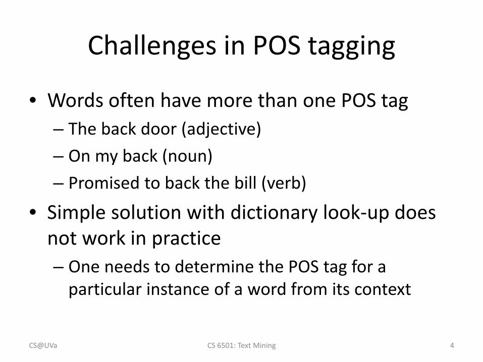
Challenges in POS tagging

• Words often have more than one POS tag– The back door (adjective)– On my back (noun)– Promised to back the bill (verb)

• Simple solution with dictionary look-up does not work in practice– One needs to determine the POS tag for a

particular instance of a word from its context


Define a tagset

• We have to agree on a standard inventory of word classes– Taggers are trained on a labeled corpora– The tagset needs to capture semantically or

syntactically important distinctions that can easily be made by trained human annotators


Word classes

• Open classes– Nouns, verbs, adjectives, adverbs

• Closed classes– Auxiliaries and modal verbs– Prepositions, Conjunctions– Pronouns, Determiners– Particles, Numerals


Public tagsets in NLP

• Brown corpus - Francis and Kucera 1961– 500 samples, distributed across 15 genres in rough

proportion to the amount published in 1961 in each of those genres

– 87 tags• Penn Treebank - Marcus et al. 1993

– Hand-annotated corpus of Wall Street Journal, 1M words

– 45 tags, a simplified version of Brown tag set– Standard for English now

• Most statistical POS taggers are trained on this Tagset


http://www.ling.upenn.edu/courses/Fall_2003/ling001/penn_treebank_pos.html

How much ambiguity is there?

• Statistics of word-tag pair in Brown Corpus and Penn Treebank

11% 18%


Is POS tagging a solved problem?

• Baseline– Tag every word with its most frequent tag– Tag unknown words as nouns– Accuracy

• Word level: 90%• Sentence level

– Average English sentence length 14.3 words– 0.914.3 = 22%

Accuracy of State-of-the-art POS Tagger• Word level: 97%• Sentence level: 0.9714.3 = 65%


Building a POS tagger

• Rule-based solution1. Take a dictionary that lists all possible tags for

each word2. Assign to every word all its possible tags3. Apply rules that eliminate impossible/unlikely

tag sequences, leaving only one tag per wordshe PRPpromised VBN,VBDto TOback VB, JJ, RB, NN!!the DTbill NN, VB

R1: Pronoun should be followed by a past tense verb

R2: Verb cannot follow determiner


Rules can be learned via inductive learning.

Building a POS tagger

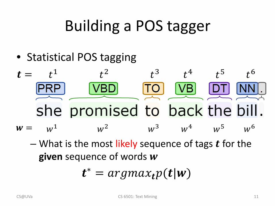
• Statistical POS tagging

– What is the most likely sequence of tags 𝒕𝒕 for the given sequence of words 𝒘𝒘

𝑡𝑡1 𝑡𝑡2 𝑡𝑡3 𝑡𝑡4 𝑡𝑡5 𝑡𝑡6

𝑤𝑤1 𝑤𝑤2 𝑤𝑤3 𝑤𝑤4 𝑤𝑤5 𝑤𝑤6

𝒕𝒕 =

𝒘𝒘 =

𝒕𝒕∗ = 𝑎𝑎𝑎𝑎𝑎𝑎𝑎𝑎𝑎𝑎𝑥𝑥𝒕𝒕𝑝𝑝(𝒕𝒕|𝒘𝒘)


POS tagging with generative models

• Bayes Rule

– Joint distribution of tags and words– Generative model

• A stochastic process that first generates the tags, and then generates the words based on these tags

𝒕𝒕∗ = 𝑎𝑎𝑎𝑎𝑎𝑎𝑎𝑎𝑎𝑎𝑥𝑥𝒕𝒕𝑝𝑝 𝒕𝒕 𝒘𝒘= 𝑎𝑎𝑎𝑎𝑎𝑎𝑎𝑎𝑎𝑎𝑥𝑥𝒕𝒕

𝑝𝑝 𝒘𝒘 𝒕𝒕 𝑝𝑝(𝒕𝒕)𝑝𝑝(𝒘𝒘)

= 𝑎𝑎𝑎𝑎𝑎𝑎𝑎𝑎𝑎𝑎𝑥𝑥𝒕𝒕𝑝𝑝 𝒘𝒘 𝒕𝒕 𝑝𝑝(𝒕𝒕)


Hidden Markov models

• Two assumptions for POS tagging1. Current tag only depends on previous 𝑘𝑘 tags

• 𝑝𝑝 𝒕𝒕 = ∏𝑖𝑖 𝑝𝑝(𝑡𝑡𝑖𝑖|𝑡𝑡𝑖𝑖−1, 𝑡𝑡𝑖𝑖−2, … , 𝑡𝑡𝑖𝑖−𝑘𝑘)• When 𝑘𝑘=1, it is so-called first-order HMMs

2. Each word in the sequence depends only on its corresponding tag• 𝑝𝑝 𝒘𝒘 𝒕𝒕 = ∏𝑖𝑖 𝑝𝑝(𝑤𝑤𝑖𝑖|𝑡𝑡𝑖𝑖)


Graphical representation of HMMs

• Light circle: latent random variables• Dark circle: observed random variables• Arrow: probabilistic dependency

𝑝𝑝(𝑡𝑡𝑖𝑖|𝑡𝑡𝑖𝑖−1) Transition probability

𝑝𝑝(𝑤𝑤𝑖𝑖|𝑡𝑡𝑖𝑖)Emission probability

All the tags in the tagset

All the words in the vocabulary


Finding the most probable tag sequence

• Complexity analysis– Each word can have up to 𝑇𝑇 tags– For a sentence with 𝑁𝑁 words, there will be up to 𝑇𝑇𝑁𝑁 possible tag sequences

– Key: explore the special structure in HMMs!

𝒕𝒕∗ = 𝑎𝑎𝑎𝑎𝑎𝑎𝑎𝑎𝑎𝑎𝑥𝑥𝒕𝒕𝑝𝑝 𝒕𝒕 𝒘𝒘

= 𝑎𝑎𝑎𝑎𝑎𝑎𝑎𝑎𝑎𝑎𝑥𝑥𝒕𝒕�𝑖𝑖

𝑝𝑝 𝑤𝑤𝑖𝑖 𝑡𝑡𝑖𝑖 𝑝𝑝(𝑡𝑡𝑖𝑖|𝑡𝑡𝑖𝑖−1)


𝑤𝑤1 𝑤𝑤2 𝑤𝑤3 𝑤𝑤4 𝑤𝑤5𝑡𝑡1𝑡𝑡2𝑡𝑡3𝑡𝑡4𝑡𝑡5𝑡𝑡6𝑡𝑡7

Word 𝑤𝑤1 takes tag 𝑡𝑡4CS@UVa CS 6501: Text Mining 16

𝒕𝒕𝟏𝟏 = 𝑡𝑡4𝑡𝑡1𝑡𝑡3𝑡𝑡5𝑡𝑡7 𝒕𝒕𝟐𝟐 = 𝑡𝑡4𝑡𝑡1𝑡𝑡3𝑡𝑡5𝑡𝑡2

Trellis: a special structure for HMMs


Word 𝑤𝑤1 takes tag 𝑡𝑡4

𝒕𝒕𝟏𝟏 = 𝑡𝑡4𝑡𝑡1𝑡𝑡3𝑡𝑡5𝑡𝑡7 𝒕𝒕𝟐𝟐 = 𝑡𝑡4𝑡𝑡1𝑡𝑡3𝑡𝑡5𝑡𝑡2Computation can be reused!


Viterbi algorithm

• Store the best tag sequence for 𝑤𝑤1 …𝑤𝑤𝑖𝑖 that ends in 𝑡𝑡𝑗𝑗 in 𝑇𝑇[𝑗𝑗][𝑖𝑖]– 𝑇𝑇[𝑗𝑗][𝑖𝑖] = max𝑝𝑝(𝑤𝑤1 …𝑤𝑤𝑖𝑖 , 𝑡𝑡1 … , 𝑡𝑡𝑖𝑖 = 𝑡𝑡𝑗𝑗 )

• Recursively compute trellis[j][i] from the entries in the previous column trellis[j][i-1]– 𝑇𝑇 𝑗𝑗 𝑖𝑖 = 𝑃𝑃 𝑤𝑤𝑖𝑖 𝑡𝑡𝑗𝑗 𝑀𝑀𝑎𝑎𝑥𝑥𝑘𝑘 𝑇𝑇 𝑘𝑘 𝑖𝑖 − 1 𝑃𝑃 𝑡𝑡𝑗𝑗 𝑡𝑡𝑘𝑘

The best i-1 tag sequence

Generating the current observation

Transition from the previous best ending tag


Viterbi algorithm



𝑇𝑇 𝑗𝑗 𝑖𝑖 = 𝑃𝑃 𝑤𝑤𝑖𝑖 𝑡𝑡𝑗𝑗 𝑀𝑀𝑎𝑎𝑥𝑥𝑘𝑘 𝑇𝑇 𝑘𝑘 𝑖𝑖 − 1 𝑃𝑃 𝑡𝑡𝑗𝑗 𝑡𝑡𝑘𝑘

Order of computation

Dynamic programming: 𝑂𝑂(𝑇𝑇2𝑁𝑁)!

Decode 𝑎𝑎𝑎𝑎𝑎𝑎𝑎𝑎𝑎𝑎𝑥𝑥𝒕𝒕𝑝𝑝(𝒕𝒕|𝒘𝒘)

• Take the highest scoring entry in the last column of the trellis


Keep backpointers in each trellis to keep track of the most probable sequence


𝑇𝑇 𝑗𝑗 𝑖𝑖 = 𝑃𝑃 𝑤𝑤𝑖𝑖 𝑡𝑡𝑗𝑗 𝑀𝑀𝑎𝑎𝑥𝑥𝑘𝑘 𝑇𝑇 𝑘𝑘 𝑖𝑖 − 1 𝑃𝑃 𝑡𝑡𝑗𝑗 𝑡𝑡𝑘𝑘

Train an HMM tagger

• Parameters in an HMM tagger– Transition probability: 𝑝𝑝 𝑡𝑡𝑖𝑖 𝑡𝑡𝑗𝑗 ,𝑇𝑇 × 𝑇𝑇– Emission probability: 𝑝𝑝 𝑤𝑤 𝑡𝑡 ,𝑉𝑉 × 𝑇𝑇– Initial state probability: 𝑝𝑝 𝑡𝑡 𝜋𝜋 ,𝑇𝑇 × 1

For the first tag in a sentence


Train an HMMs tagger

• Maximum likelihood estimator– Given a labeled corpus, e.g., Penn Treebank– Count how often we have the pair of 𝑡𝑡𝑖𝑖𝑡𝑡𝑗𝑗 and 𝑤𝑤𝑖𝑖𝑡𝑡𝑗𝑗

• 𝑝𝑝 𝑡𝑡𝑗𝑗 𝑡𝑡𝑖𝑖 = 𝑐𝑐(𝑡𝑡𝑖𝑖,𝑡𝑡𝑗𝑗)𝑐𝑐(𝑡𝑡𝑖𝑖)

• 𝑝𝑝 𝑤𝑤𝑖𝑖 𝑡𝑡𝑗𝑗 = 𝑐𝑐(𝑤𝑤𝑖𝑖,𝑡𝑡𝑗𝑗)𝑐𝑐(𝑡𝑡𝑗𝑗)


Proper smoothing is necessary!

Public POS taggers• Brill’s tagger

– http://www.cs.jhu.edu/~brill/ • TnT tagger

– http://www.coli.uni-saarland.de/~thorsten/tnt/• Stanford tagger

– http://nlp.stanford.edu/software/tagger.shtml• SVMTool

– http://www.lsi.upc.es/~nlp/SVMTool/• GENIA tagger

– http://www-tsujii.is.s.u-tokyo.ac.jp/GENIA/tagger/• More complete list at

– http://www-nlp.stanford.edu/links/statnlp.html#Taggers


Let’s take a look at other NLP tasks

• Noun phrase (NP) chunking– Task: identify all non-recursive NP chunks


The BIO encoding

• Define three new tags– B-NP: beginning of a noun phrase chunk– I-NP: inside of a noun phrase chunk– O: outside of a noun phrase chunk

POS Tagging with a restricted Tagset?


Another NLP task

• Shallow parsing– Task: identify all non-recursive NP, verb (“VP”) and

preposition (“PP”) chunks


BIO Encoding for Shallow Parsing

• Define several new tags– B-NP B-VP B-PP: beginning of an “NP”, “VP”, “PP” chunk– I-NP I-VP I-PP: inside of an “NP”, “VP”, “PP” chunk– O: outside of any chunk



Yet another NLP task

• Named Entity Recognition– Task: identify all mentions of named entities

(people, organizations, locations, dates)


BIO Encoding for NER

• Define many new tags– B-PERS, B-DATE,…: beginning of a mention of a

person/date...– I-PERS, B-DATE,…: inside of a mention of a person/date...– O: outside of any mention of a named entity



Sequence labeling

• Many NLP tasks are sequence labeling tasks– Input: a sequence of tokens/words– Output: a sequence of corresponding labels

• E.g., POS tags, BIO encoding for NER

– Solution: finding the most probable label sequence for the given word sequence

• 𝒕𝒕∗ = 𝑎𝑎𝑎𝑎𝑎𝑎𝑎𝑎𝑎𝑎𝑥𝑥𝒕𝒕𝑝𝑝 𝒕𝒕 𝒘𝒘


Comparing to traditional classification problem

Sequence labeling• 𝒕𝒕∗ = 𝑎𝑎𝑎𝑎𝑎𝑎𝑎𝑎𝑎𝑎𝑥𝑥𝒕𝒕𝑝𝑝 𝒕𝒕 𝒘𝒘

– 𝒕𝒕 is a vector/matrix

• Dependency between both (𝒕𝒕,𝒘𝒘) and (𝑡𝑡𝑖𝑖 , 𝑡𝑡𝑗𝑗)

• Structured output • Difficult to solve the

inference problem

Traditional classification • 𝑦𝑦 = 𝑎𝑎𝑎𝑎𝑎𝑎𝑎𝑎𝑎𝑎𝑥𝑥𝑦𝑦𝑝𝑝(𝑦𝑦|𝒙𝒙)

– 𝑦𝑦 is a single label

• Dependency only within (𝑦𝑦,𝒙𝒙)

• Independent output• Easy to solve the inference

problem


yi

xi xj

yjti

wi wj

tj

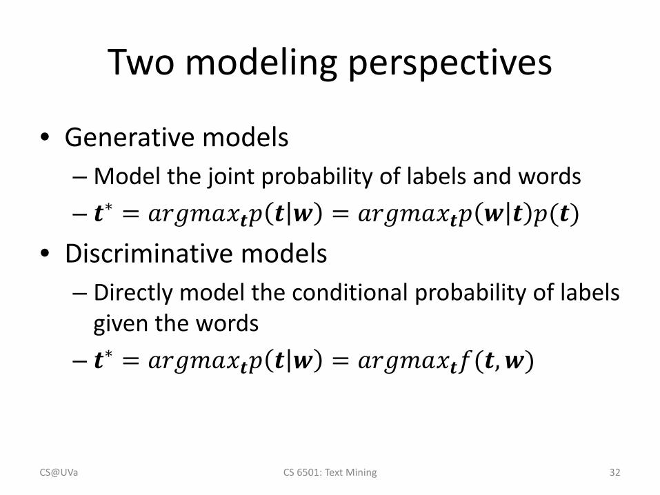
Two modeling perspectives

• Generative models– Model the joint probability of labels and words– 𝒕𝒕∗ = 𝑎𝑎𝑎𝑎𝑎𝑎𝑎𝑎𝑎𝑎𝑥𝑥𝒕𝒕𝑝𝑝 𝒕𝒕 𝒘𝒘 = 𝑎𝑎𝑎𝑎𝑎𝑎𝑎𝑎𝑎𝑎𝑥𝑥𝒕𝒕𝑝𝑝 𝒘𝒘 𝒕𝒕 𝑝𝑝(𝒕𝒕)

• Discriminative models– Directly model the conditional probability of labels

given the words– 𝒕𝒕∗ = 𝑎𝑎𝑎𝑎𝑎𝑎𝑎𝑎𝑎𝑎𝑥𝑥𝒕𝒕𝑝𝑝 𝒕𝒕 𝒘𝒘 = 𝑎𝑎𝑎𝑎𝑎𝑎𝑎𝑎𝑎𝑎𝑥𝑥𝒕𝒕𝑓𝑓(𝒕𝒕,𝒘𝒘)


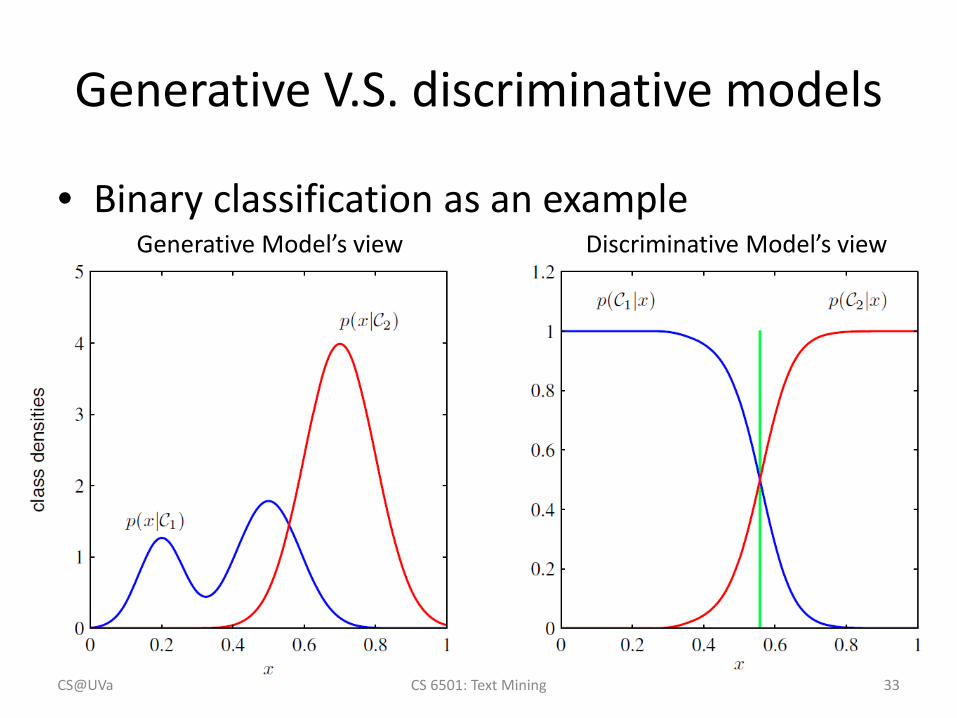
Generative V.S. discriminative models

• Binary classification as an example


Generative Model’s view Discriminative Model’s view

Generative V.S. discriminative models

Generative• Specifying joint distribution

– Full probabilistic specification for all the random variables

• Dependence assumption has to be specified for 𝑝𝑝 𝒘𝒘 𝒕𝒕 and 𝑝𝑝(𝒕𝒕)

• Flexible, can be used in unsupervised learning

Discriminative • Specifying conditional

distribution– Only explain the target

variable

• Arbitrary features can be incorporated for modeling 𝑝𝑝 𝒕𝒕 𝒘𝒘

• Need labeled data, only suitable for (semi-) supervised learning


Maximum entropy Markov models

• MEMMs are discriminative models of the labels 𝒕𝒕 given the observed input sequence 𝒘𝒘– 𝑝𝑝 𝒕𝒕 𝒘𝒘 = ∏𝑖𝑖 𝑝𝑝(𝑡𝑡𝑖𝑖|𝑤𝑤𝑖𝑖 , 𝑡𝑡𝑖𝑖−1)


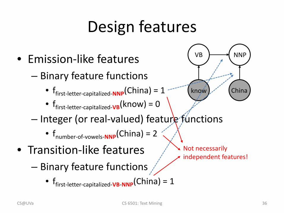
Design features

• Emission-like features– Binary feature functions

• ffirst-letter-capitalized-NNP(China) = 1• ffirst-letter-capitalized-VB(know) = 0

– Integer (or real-valued) feature functions• fnumber-of-vowels-NNP(China) = 2

• Transition-like features– Binary feature functions

• ffirst-letter-capitalized-VB-NNP(China) = 1

Not necessarily independent features!

VB

China

NNP


know

Parameterization of 𝑝𝑝(𝑡𝑡𝑖𝑖|𝑤𝑤𝑖𝑖 , 𝑡𝑡𝑖𝑖−1)

• Associate a real-valued weight 𝜆𝜆 to each specific type of feature function– 𝜆𝜆𝑘𝑘 for ffirst-letter-capitalized-NNP(w)

• Define a scoring function 𝑓𝑓 𝑡𝑡𝑖𝑖 , 𝑡𝑡𝑖𝑖−1,𝑤𝑤𝑖𝑖 =∑𝑘𝑘 𝜆𝜆𝑘𝑘𝑓𝑓𝑘𝑘(𝑡𝑡𝑖𝑖 , 𝑡𝑡𝑖𝑖−1,𝑤𝑤𝑖𝑖)

• Naturally 𝑝𝑝 𝑡𝑡𝑖𝑖 𝑤𝑤𝑖𝑖 , 𝑡𝑡𝑖𝑖−1 ∝ exp 𝑓𝑓 𝑡𝑡𝑖𝑖 , 𝑡𝑡𝑖𝑖−1,𝑤𝑤𝑖𝑖– Recall the basic definition of probability

• 𝑃𝑃(𝑥𝑥) > 0• ∑𝑥𝑥 𝑝𝑝(𝑥𝑥) = 1


Parameterization of MEMMs

• It is a log-linear model– log 𝑝𝑝 𝒕𝒕 𝒘𝒘 = ∑𝑖𝑖 𝑓𝑓(𝑡𝑡𝑖𝑖 , 𝑡𝑡𝑖𝑖−1,𝑤𝑤𝑖𝑖) − 𝐶𝐶(𝝀𝝀)

• Viterbi algorithm can be used to decode the most probable label sequence solely based on ∑𝑖𝑖 𝑓𝑓(𝑡𝑡𝑖𝑖 , 𝑡𝑡𝑖𝑖−1,𝑤𝑤𝑖𝑖)

𝑝𝑝 𝒕𝒕 𝒘𝒘 = �𝑖𝑖

𝑝𝑝(𝑡𝑡𝑖𝑖|𝑤𝑤𝑖𝑖 , 𝑡𝑡𝑖𝑖−1)

=∏𝑖𝑖 exp 𝑓𝑓(𝑡𝑡𝑖𝑖 , 𝑡𝑡𝑖𝑖−1,𝑤𝑤𝑖𝑖)∑𝒕𝒕∏𝑖𝑖 exp 𝑓𝑓(𝑡𝑡𝑖𝑖 , 𝑡𝑡𝑖𝑖−1,𝑤𝑤𝑖𝑖)

Constant only related to 𝝀𝝀


Parameter estimation

• Maximum likelihood estimator can be used in a similar way as in HMMs– 𝜆𝜆∗ = 𝑎𝑎𝑎𝑎𝑎𝑎𝑎𝑎𝑎𝑎𝑥𝑥𝜆𝜆 ∑𝒕𝒕,𝑤𝑤 log 𝑝𝑝(𝒕𝒕|𝑤𝑤)

= 𝑎𝑎𝑎𝑎𝑎𝑎𝑎𝑎𝑎𝑎𝑥𝑥𝜆𝜆�𝒕𝒕,𝑤𝑤

�𝑖𝑖

𝑓𝑓(𝑡𝑡𝑖𝑖 , 𝑡𝑡𝑖𝑖−1,𝑤𝑤𝑖𝑖) − 𝐶𝐶(𝝀𝝀)

Decompose the training data into such units


Why maximum entropy?

• We will explain this in detail when discussing the Logistic Regression models


A little bit more about MEMMs

• Emission features can go across multiple observations– 𝑓𝑓 𝑡𝑡𝑖𝑖 , 𝑡𝑡𝑖𝑖−1,𝑤𝑤𝑖𝑖 ≜ ∑𝑘𝑘 𝜆𝜆𝑘𝑘𝑓𝑓𝑘𝑘(𝑡𝑡𝑖𝑖 , 𝑡𝑡𝑖𝑖−1,𝒘𝒘)– Especially useful for shallow parsing and NER tasks


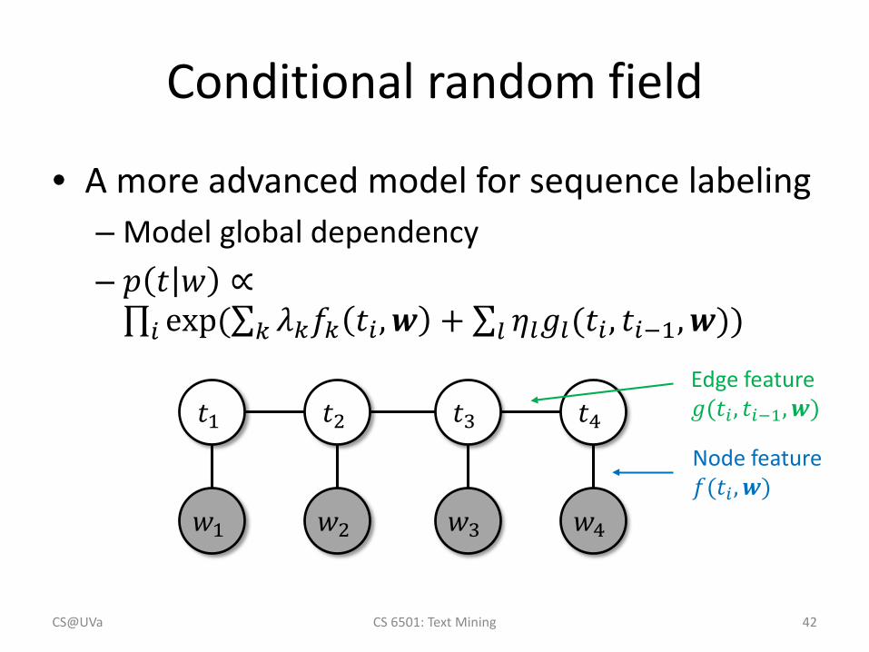
Conditional random field

• A more advanced model for sequence labeling– Model global dependency– 𝑝𝑝 𝑡𝑡 𝑤𝑤 ∝∏𝑖𝑖 exp(∑𝑘𝑘 𝜆𝜆𝑘𝑘𝑓𝑓𝑘𝑘 𝑡𝑡𝑖𝑖 ,𝒘𝒘 + ∑𝑙𝑙 𝜂𝜂𝑙𝑙𝑎𝑎𝑙𝑙(𝑡𝑡𝑖𝑖 , 𝑡𝑡𝑖𝑖−1,𝒘𝒘))

𝑡𝑡3 𝑡𝑡4

𝑤𝑤3 𝑤𝑤4

𝑡𝑡1 𝑡𝑡2

𝑤𝑤1 𝑤𝑤2

Node feature 𝑓𝑓(𝑡𝑡𝑖𝑖 ,𝒘𝒘)

Edge feature 𝑎𝑎(𝑡𝑡𝑖𝑖 , 𝑡𝑡𝑖𝑖−1,𝒘𝒘)


What you should know

• Definition of POS tagging problem– Property & challenges

• Public tag sets• Generative model for POS tagging

– HMMs

• General sequential labeling problem• Discriminative model for sequential labeling

– MEMMs


Today’s reading

• Speech and Language Processing– Chapter 5: Part-of-Speech Tagging– Chapter 6: Hidden Markov and Maximum Entropy

Models– Chapter 22: Information Extraction (optional)


part-of-speech tagging & sequence labeling

Documents