Part-of-Speech Tagging for Twitter: Word Clusters andOther Advances

Olutobi Owoputi∗ Brendan O’Connor∗ Chris Dyer∗Kevin Gimpel† Nathan Schneider∗

September 2012CMU-ML-12-107

School of Computer ScienceCarnegie Mellon University

Pittsburgh, PA 15213

∗ School of Computer Science, Carnegie Mellon University† Toyota Technological Institute at Chicago, Chicago, IL 60637

Abstract

We present improvements to a Twitter part-of-speech tagger, making use of several new features and large-scale word clustering. With these changes, the tagging accuracy increased from 89.2% to 92.8% and thetagging speed is 40 times faster. In addition, we expanded our Twitter tokenizer to support a broader rangeof Unicode characters, emoticons, and URLs. Finally, we annotate and evaluate on a new tweet dataset,DAILYTWEET547, that is more statistically representative of English-language Twitter as a whole. The newtagger is released as TweetNLP version 0.3, along with the new annotated data and large-scale word clustersat http://www.ark.cs.cmu.edu/TweetNLP.

This research was supported in part by an REU supplement to NSF grant IIS-0915187 and Google’s support of the WorldlyKnowledge project at CMU.

Keywords: part-of-speech tagging, social media, semi-supervised learning, natural language processing

1 Introduction

We extend the Twitter part-of-speech tagger that was developed in [Gimpel et al.2011]. It used a feature-based sequence tagging model with several broad types of orthographic, lexical, and distributional features.

The new part-of-speech tagger has a more efficient model implementation, and a variety of new features.This paper describes the improvements made to the tokenizer, the new lexical features, and the new distri-butional features based on unsupervised hierarchical clustering from a much larger amount of unlabeleddata. Finally, the paper compares the speed and accuracy between the two versions in different domains andsuggests possible future improvements to the tagger.

2 Tokenizer Improvements

Tokenization is a challenging problem for Twitter text. In addition to traditional words, our tokenizer alsorecognizes URLs and emoticons. These are important to preserve for many text analysis applications.

The original Twitter part-of-speech tagger used a Scala port of “Twokenize” [O’Connor et al.2010]. Forthe new tagger, we ported the tokenizer to Java for fewer dependencies. The tokenizer can process about3500 tweets per second.

We added support for numbers with multiple dots, commas, and colons (533.124.2412 12:12:12 etc.)and currency. The tokenizer still occasionally makes errors with commas and numbers; for example, it isdifficult to disambiguate between “check out tracks 1,3,5,10.” and “Wind 8,3 km/h SSW”.

We added support for Eastern-style horizontal emoticons (e.g. o.o - -) to the tokenizer. However, sincemany of these emoticons use characters from other language character sets, the patterns may cause tokeniza-tion errors on languages other than English.

We changed the tokenizer URL pattern to recognize valid links from top level and country domains,which is necessary for the ambiguous case where the protocol (e.g. http:// ) is omitted. One issue is that thethis pattern matches tokens like w.me, yup.am, come.in, home.my, ever.be etc. which could be valid URLsbut are actually two word phrases without punctuation. However, these are very rare.

Another possible issue regarding URL tokenization is with the upcoming expansion of the number ofgeneric Top-Level-Domains from 22 to potentially over 2,000.1 These changes will add to the ambiguitybetween URLs and phrases when the protocol is omitted and will require both Twitter and the tokenizer toupdate URL detection patterns. It may eventually be necessary to use statistical disambiguation.

3 Proper Noun Recognition

Proper noun tokens were accurately labeled only 71% of the time in the original tagger, most often confusedwith nouns. The task of recognizing proper nouns is especially difficult with Twitter, as neither correctcapitalization nor spelling can be used as reliable indicators.

3.1 Dictionary Lists

The original tagger used a soft-constraint tag dictionary generated from the WSJ and Brown Penn Treebankcorpora. However, the dictionary seemed to have limited effectiveness in proper noun detection, since the

1http://newgtlds.icann.org/en/program-status/application-results/strings-1200utc-13jun12-en

1

many of the proper nouns/names in the corpora are from the 1960s/1980s and are not commonly seen in thedomain of Twitter conversations.

3.2 Name Lists

We added several name lists to the tagger with the hope of improving proper noun recognition. The listsinclude the Freebase celebrities and video games lists, the Moby Words list of US Locations,2 and lists ofmale, female, family, and proper names from Mark Kantrowitz’s name corpus.3

We removed the old taggers’ name list of frequently capitalized tokens, since it did not improve accuracy.(It may be worth revisiting with more data.)

4 Orthographic Features

We expanded the taggers’ orthographic features. The regular expression features for whether or not a tokenmatched a valid URL or emoticon were updated to the improved patterns from the tokenizer (section 2).

The tagger model uses word shapes as features. We added the traditional (uppercase, lowercase, digit)word shape feature as well as a feature that maps each character to its Unicode character category. Inaddition, the token n-gram suffix features were increased from n ≤ 3 to n ≤ 20 and n-gram prefix featuresof the same size were added.

5 Other changes

We removed the lexical features based on Metaphone phonetic normalization of words, which were notuseful given our other features. We did, however, retain the Metaphone normalized PTB tag lookup feature;it seemed to help a small amount beyond direct lookup.

We added linear position features: for every token we include two feature indicators for its position t thetoken: an indicator for the distance from the start, and the distance from the end. L1 regularization selectsto only the first few positions having nonzero weights.

6 Word Clustering

Given that previous work has found word clusters to improve the performance of supervised NLP models(e.g. [Turian et al.2010]), we constructed features from hierarchical word clustering on a large set of un-labeled tweets. This section explains the clustering methodology as well as the effects of using the wordclusters as features.

6.1 Methodology

For tweet clustering, we used Percy Liang’s implementation of Brown clustering [Liang2005, Brown et al.1992],4

which is an HMM-based algorithm that partitions words into a base set of 1000 clusters, and induces a hier-archy among those 1000 clusters.

2http://icon.shef.ac.uk/Moby/mwords.html3http://www.cs.cmu.edu/afs/cs/project/ai-repository/ai/areas/nlp/corpora/names/0.

html4Version 1.3: https://github.com/percyliang/brown-cluster

2

In order to remove time-specific biases, for the unlabeled data we took a random sample of 100,000tweets per day from September 10, 2008 to August 14, 2012 and filtered out non-English tweets (about 60%of the sample) using langid.py [Lui and Baldwin2012].5 We applied a normalization step to each tweet, con-verting tweets to lowercase, at-mentions to <@MENTION>, and URLs/email addresses to their domains(e.g. http://bit.ly/dP8rR8⇒<URL-bit.ly>). Finally, the cleaning step involved removing duplicated tweetsin an effort to remove spam that could influence the clusters. The 100,000 daily sample resulted in 56 mil-lion unique tweets (847 million tokens) after normalization and cleaning. We set the clustering software’scount threshold to only cluster words appearing 40 or more times. It clustered 216,856 word types into 1000clusters, which took 42 hours.

6.2 Improvements Over DistSim

The word cluster features that we used differ from the distributional similarity features used in the originaltagger (DistSim) in several ways. DistSim calculated a word transition matrix from unlabelled data andused singular value decomposition to associate each word with a latent 50-dimensional vector, using eachdimension as a lexical feature. Since Brown clusters are hierarchical in a binary tree, each word is associatedwith a bitstring (tree path) with length ≤16, and prefixes of the bitstring are used as features.

Additionally, we found that taking tweets sampled from a long span of time was more effective thanonly clustering tweets from over just a few days, since it resulted in increased lexical coverage and fewerdate-specific errors (e.g. numerical dates appearing in the same cluster as the word ‘tonight’). Also, theamount of unannotated data used is much larger, from 134k to 56m tweets. (It would be interesting to testembeddings’ performance when trained on this larger dataset.) Finally, when checking to see if a word isassociated with a cluster, the tagger creates a priority list of fuzzy match transformations of the word byremoving repeated punctuation and repeated characters. If the original word is not in a cluster, the taggerthen considers the fuzzy matches. This method resulted in a relative error decrease of 18% among wordsnot in a cluster.

6.3 Emoticons

The Brown clusters from unlabeled tweets grouped similar emoticons together. We observed separate emoti-con clusters of happy (e.g. :) =) ∧ ∧ ), sad/disappointed (e.g. :/ :( - - </3 ), love (e.g. Œxoxo Œ.Œ) andwinking (e.g. ;) (∧ -) ). The clusters were not perfect, however. For example, the sad emoticon clusterincluded things like #tear and #ugh (which might be reasonable for an emotion detection task, but our tags’conventions treat them separately). Some emoticons were added to other unrelated groups, but the majoritywere clustered correctly.

One difficult task is classifying symbols in tweets as emoticons, punctuation or garbage. Several Uni-code character ranges define symbols and emoticons; however, depending on the font one uses, charactersin these ranges might appear differently or not at all. Clustering has helped the tagger in this task, as mostiOS symbol emoticons are grouped in the same clusters as normal emoticons. For example the characterU+E056 which is interpreted on iOS as a smiling face, is in the same cluster as the emoticon ‘:)’. Thesymbol U+E12F, which represents a bag of money, is grouped with the words ‘cash’ and ‘money’. Thesegroupings were useful in improving emoticon accuracy and could have applications in sentiment analysis ofsocial media.

5https://github.com/saffsd/langid.py

3

Celebrities 80.0%Male Names 68.9%Video Games 60.3%Female Names 39.7%Family Names 26.0%Moby Dict. Places 18.7%Proper Names 11.1%

Table 1: Cluster lexical coverage of name lists

N.Tweets N.Tokens TimespanOCT27 1827 26594 2010-10-27 and 2010-10-28DAILY547 547 7707 2011-01-01 through 2012-06-30NPSCHAT 7935 37081 2006-10 and 2006-11

Table 2: Annotated datasets

6.4 Proper Nouns

Word clustering has resulted in some improvements in recognizing names. Table 1 shows the clusters’lexical coverage of each of the name lists (i.e. words that occur at least 40 times in the 6 million tweets).But since the clustering algorithm makes hard decisions for individual word types, the tagger still strugglesto identify named entity phrases that include common words such as names of television shows and movies.

7 New annotations and evaluation set

The original dataset [Gimpel et al.2011] consisted almost entirely of tweets sampled from one particularday (October 27, 2010), and we were concerned the model might be overfit to time-specific phenomena; forexample, a substantial fraction of the messages are about a basketball game happening that day.

A new test set of 547 tweets was created for evaluation. The test set consists of one random Englishtweet from every day between January 1, 2011 and June 30, 2012. In order for a tweet to be consideredEnglish, it had to contain at least one English word other than a URL, emotion, or mention. We noticedbiases in the outputs of the langid.py tool, so we found and verified these messages manually.

The tweets were annotated by two annotators with experience from the previous annotation effort. Dif-ferences were reconciled by a third annotator in discussion with all annotators, and the annotation guidelineswere updated accordingly.6 We found one issue where we discovered an inconsistency in the previous ver-sion of the original data (tagging of this/that); we updated the original data and include a copy of it (OCT27),as well as the new DAILY547 dataset, in the new 0.3 release of the annotated data. (Only 100 (0.4%) of thelabels have changed.) The new release of the tagger includes a model trained on all the available data.

6Included with the tagger, and accessible online at https://github.com/brendano/ark-tweet-nlp/blob/master/docs/annot_guidelines.md

4

Feature set OCT27TEST DAILY547 NPSCHAT

All features 0.9160 0.9280 0.9119with clusters; without tagdicts, namelists 0.9115 0.9238 0.9066without clusters; with tagdicts, namelists 0.8981 0.9081 0.9000only clusters (and transtions) 0.8950 0.9054 0.8955without clusters, tagdicts, namelists 0.8686 0.8823 0.8826

Old tagger (version 0.2), best model 0.8889 0.8917Interannotator agreement [Gimpel et al.2011] 0.922

Table 3: Tagging accuracy results, for models only trained on OCT27TRAIN+DEV, and ablations involv-ing lexicon features. Note OCT27TEST and DAILY547 95% confidence intervals are roughly ±0.007(≈ 1.96

√0.9(0.1)/ntok).

Tag Acc Confused Tag Acc ConfusedV 94 N ! 87 NN 90 ˆ L 94 O D, 99 ˜ & 95 ,P 95 R U 98 , Gˆ 76 N $ 89 A PD 97 O # 90 NO 98 D G 24 ,A 84 V E 90 ,R 87 P T 72 P@ 99 P ˆ Z 23 ˆ˜ 94 ,

Table 4: Accuracy (recall) rates per tag and the most commonly confused tag on the OCT27 test set. Multipletags indicate a tie.

8 Results

The new version of the part-of-speech tagger shows significant improvements in speed and accuracy overthe original tagger.

8.1 Speed

The original part-of-speech tagger processed about 18-20 tweets and 200 tokens per second, while thenew version tags around 800 tweets and 10,000 tokens per second (3 million tweets/hour). Some of thisimprovement is due to algorithmic differences; see section 9. The tokenizer by itself runs at about 3500tweets per second (12 million tweets/hour). Timings on an Intel Core i5 2.4 GHz laptop.

8.2 Accuracy

The new test set is easier: the full tagger, trained on all of OCT27, attains 93.2% accuracy. To comparedifferent settings of the tagger, we train it on OCT27’s training and development sets, then report test resultson both OCT27TEST and all of DAILY547. Results are shown in Table 3.

5

●

●

●

● ● ● ●

1e+03 1e+05 1e+07

7580

8590

Number of Unlabeled Tweets

Tagg

ing

Acc

urac

y

●

●

●●

● ● ●

1e+03 1e+05 1e+07

0.60

0.65

0.70

Number of Unlabeled Tweets

Toke

n C

over

age

●

●

●

● ● ● ●

1e+03 1e+05 1e+07

7580

8590

Number of Unlabeled Tweets

Tagg

ing

Acc

urac

y

●

●

●●

● ● ●

1e+03 1e+05 1e+07

0.60

0.65

0.70

Number of Unlabeled Tweets

Toke

n C

over

age

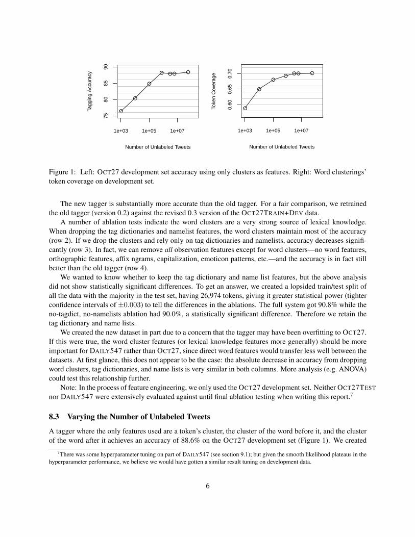
Figure 1: Left: OCT27 development set accuracy using only clusters as features. Right: Word clusterings’token coverage on development set.

The new tagger is substantially more accurate than the old tagger. For a fair comparison, we retrainedthe old tagger (version 0.2) against the revised 0.3 version of the OCT27TRAIN+DEV data.

A number of ablation tests indicate the word clusters are a very strong source of lexical knowledge.When dropping the tag dictionaries and namelist features, the word clusters maintain most of the accuracy(row 2). If we drop the clusters and rely only on tag dictionaries and namelists, accuracy decreases signifi-cantly (row 3). In fact, we can remove all observation features except for word clusters—no word features,orthographic features, affix ngrams, capitalization, emoticon patterns, etc.—and the accuracy is in fact stillbetter than the old tagger (row 4).

We wanted to know whether to keep the tag dictionary and name list features, but the above analysisdid not show statistically significant differences. To get an answer, we created a lopsided train/test split ofall the data with the majority in the test set, having 26,974 tokens, giving it greater statistical power (tighterconfidence intervals of ±0.003) to tell the differences in the ablations. The full system got 90.8% while theno-tagdict, no-namelists ablation had 90.0%, a statistically significant difference. Therefore we retain thetag dictionary and name lists.

We created the new dataset in part due to a concern that the tagger may have been overfitting to OCT27.If this were true, the word cluster features (or lexical knowledge features more generally) should be moreimportant for DAILY547 rather than OCT27, since direct word features would transfer less well between thedatasets. At first glance, this does not appear to be the case: the absolute decrease in accuracy from droppingword clusters, tag dictionaries, and name lists is very similar in both columns. More analysis (e.g. ANOVA)could test this relationship further.

Note: In the process of feature engineering, we only used the OCT27 development set. Neither OCT27TEST

nor DAILY547 were extensively evaluated against until final ablation testing when writing this report.7

8.3 Varying the Number of Unlabeled Tweets

A tagger where the only features used are a token’s cluster, the cluster of the word before it, and the clusterof the word after it achieves an accuracy of 88.6% on the OCT27 development set (Figure 1). We created

7There was some hyperparameter tuning on part of DAILY547 (see section 9.1); but given the smooth likelihood plateaus in thehyperparameter performance, we believe we would have gotten a similar result tuning on development data.

6

several clusterings with different amounts of unlabeled tweets, keeping the number of clusters constantat 800. Initially there was a logarithmic relation between number of tweets and accuracy, but from from750 thousand to 56 million tweets, the tagging accuracy remained relatively constant. We use the largestclustering (which, unlike the others, uses 1000 clusters) as the default for the released tagger.

8.4 Evaluation on NPSCHAT

In addition to the two annotated Twitter datasets, we ran our tagger on the NPS Chat Corpus[Forsyth and Martell2007],8 a Penn Treebank part-of-speech tag annotated dataset of Internet Relay Chat(IRC) room messages from 2006. We chose the dataset because IRC text often contains the same emoticons,misspellings, abbreviations and acronyms as Twitter data.

After filtering out system messages, we split the data into a training set of 5067 messages and a test setof 2868 messages. The full tagger model achieved an accuracy of 91.2% on the test set. For comparison, thebest result we could find reported in [Forsyth and Martell2007, Forsyth2007] seems to be 90.7% accuracyfrom a tagger trained on a mix of several PTB-POS-annotated corpora9

9 Algorithmic Changes

Version 0.2 of the tagger used a first-order chain conditional random field (CRF) [Lafferty et al.2001], reusedfrom a large body of experimental code. Unfortunately, it was very slow. Since an important goal is torun the tagger on millions to billions of tweets, we wrote a new, simple implementation of a first-ordermaximum entropy Markov model (MEMM) [McCallum et al.2000], which runs 30 to 40 times faster thanthe old tagger, and performs similarly. It is also much faster than a CRF to train, which is useful for quicklyexperimenting with new features.

At training time, the log-likelihood is the sum over the Ncorpus token tags yt in the training corpus, eachconditional on the observed previous tag (with an artificial start symbol as the predecessor to the first tokenin a tweet),

`(β) =

Ncorpus∑t

log p(yt | yt−1, x, β)

where the conditional probability is a multiclass logistic regression conditioning on features using yt, yt−1,as well as arbitrary features of the entire sentence (tweet) x. We use transition features for every pair oflabels, and extract base observation features from token t and neighboring tokens, and conjoin them againstall possible tag outputs.

p(yt = k | yt−1, x, β) ∝ exp

β(trans)yt−1,k+∑j

β(obs)j,k fj(x, t)

9.1 Training and elastic net regularization

We train with OWL-QN, an L1-capable variant of L-BFGS [Andrew and Gao2007, Liu and Nocedal1989]to minimize the regularized objective

8Release 1.0: http://faculty.nps.edu/cmartell/NPSChat.htm9The difference appears significant: p = .0502, for exact binomial test for our test set being 13267 tokens, against null hypoth-

esis of 0.907.

7

argminβ− 1

N`(β) +R(β)

and use elastic net regularization [Zou and Hastie2005], which simply means a mixture of L1 and L2 penal-ties; here j indexes over all final conjoined features:

R(β) = λ1∑j

|βj |+1

2λ2

∑j

β2j

Using even a very small L1 penalty eliminates many irrelevant or highly noisy features. We conducted agrid search for the regularizer values, evaluating with both likelihood and accuracy (Figure 2). Interestingly,the likelihood results are much smoother; we suspect this happens since the differences in tagging decisionsare quite small (as few as a dozen labels might change between parameter settings), so accuracy is not verysensitive due to its discrete nature—unlike likelihood. Furthermore, there is an odd phenomenon of higheraccuracy at extreme regularizer combinations; we wonder if this is an anomaly (perhaps due to the fact theL-BFGS convergence threshold was laxer for these experiments than the accuracy results in Table 3).

In any case, many regularizer values give the best or nearly the best results. We choose λ1, λ2 =(0.25, 2) achieving 93.2% accuracy (on a subset of DAILY547). There are lower L1 regularizers that give asgood or very slightly better results; however, they have much larger models, and to help ensure generalizationit may be better to err on the side of caution (sparser models). The total number of features is 3.7 million, allof which are used under pure L2; but only 60,000 are selected under (0.25, 2). It is possible to get radicallysmaller models: (4, .06) has 92.6% accuracy with only 1632 features, a small enough number to browsethrough manually.

9.2 Decoding

To tag a new tweet, the inference problem can be stated as finding the maximally likely tag sequence for asentence (tweet) with Ntweet tokens,

arg maxy1..yNtweet

Ntweet∑t

log p(yt | yt−1, x, β)

Since this decomposes into clique potentials of neighboring tags, it may be optimally solved with Viterbidecoding in O(NK2) time. However, we also experimented with greedy decoding in a single left-to-rightpass (O(NK) time):

For t = 1..T :Set yt := argmaxk log p(yt = k | yt−1, x, β)

In our implementation, greedy decoding is 3 times faster and yields similar accuracy (decreases by less than0.1% absolute on DAILY547, not significant with McNemar’s test), so we enable it by default. Accuracyresults in this document are reported with Viterbi decoding unless otherwise noted.

8

10 Confidence calibration

We call a probabilistic model is calibrated if, when its predicted probability for a label is X%, the empiricalprobability is also X%. This can be formalized in a frequentist manner as the fraction of examples havingthe label among all model predictions in the interval [X − ε,X + ε]. This implies that when the classifier isX% confident, it actually has a X% accuracy rate. It has been observed that probabilistic NLP systems cangive overly confident predictions (e.g. [Lin et al.2009]).

We tested the MEMM’s calibration. We use the greedy decoding algorithm, while saving the proba-bilities at each step, and output the probability of the most likely tag. Running on test data, we bucket thepredictions by confidence, and plot in Figure 3 the accuracy rate among predictions in that bucket, againstthe average confidence of the bucket. (Since the distribution of confidences is very skewed, we use a dy-namic bucketing technique: iterate through the predictions in decreasing confidence order, creating a newbucket once there are sufficient examples for a small standard error of estimating the accuracy rate.) If con-fidences are well-calibrated, the bucket’s average confidence should be the same as its accuracy rate. Theconfidences look to be quite well calibrated; therefore we output them by default. (Disabling them resultsin a ∼5% speedup.)

11 Future Work

There are many more possible improvements for the tagger.Unsupervised word clustering was found to be a very effective feature. A number of other techniques,

including the low-rank SVD used in the old tagger, could be explored on larger unlabeled datasets.Using more tag context (e.g. second or higher order) might be very helpful, especially given that previous

work on part-of-speech tagging has found that second-order models are useful. In the MEMM framework,it’s easy to train with unlimited history (provided you are OK with heuristic decoding); L1 regularizationmay be able to select a subset of informative long left contexts.

Right tag contexts would also be helpful, but an MEMM does not allow them. Switching to a CRF ora structured perceptron/SVM is one option. Another is to add in a separately trained right-to-left MEMM,and combine the two models’ predictions. (This idea is related to the cyclic dependency networks used in[Toutanova et al.2003]). This would preserve the fast runtime of higher order models.

Applying the word clusters to syntactic analysis in other informal domains beyond Twitter and IRC isanother possibility. For web and email data, there exists the new Google Web Treebank.10

Acknowledgements

OO implemented most of the new features and their analysis; BO implemented most of the new tagger andadditional analysis; CD helped with word clustering and the assembling the DAILY547 dataset; KG and NSannotated it and wrote the new guidelines. Thanks to Noah Smith for additional support, and again all theoriginal 2011 annotators: Desai Chen, Dipanjan Das, Chris Dyer, Jacob Eisenstein, Jeff Flanigan, Kevin Gimpel,Michael Heilman, Lori Levin, Daniel Mills, Behrang Mohit, Brendan O’Connor, Bryan Routledge, Naomi Saphra,Nathan Schneider, Noah Smith, Tae Yano, and Dani Yogatama.

10http://www.ldc.upenn.edu/Catalog/CatalogEntry.jsp?catalogId=LDC2012T13

9

References

[Andrew and Gao2007] G. Andrew and J. Gao. 2007. Scalable training of l1-regularized log-linear models.In Proceedings of the 24th International Conference on Machine Learning, page 3340.

[Brown et al.1992] P. F. Brown, P. V. de Souza, R. L. Mercer, V. J. Della Pietra, and J. C. Lai. 1992.Class-based n-gram models of natural language. Computational Linguistics, 18(4):467–479.

[Forsyth and Martell2007] E. N. Forsyth and C. H. Martell. 2007. Lexical and discourse analysis of onlinechat dialog. In Semantic Computing, 2007. ICSC 2007. International Conference on, page 1926.

[Forsyth2007] E. N. Forsyth. 2007. Improving automated lexical and discourse analysis of online chatdialog. Master’s thesis, Monterey, California Naval Postgraduate School.

[Gimpel et al.2011] K. Gimpel, N. Schneider, B. O’Connor, D. Das, D. Mills, J. Eisenstein, M. Heilman,D. Yogatama, J. Flanigan, and N. A. Smith. 2011. Part-of-speech tagging for Twitter: Annotation,features, and experiments. In Proc. ACL.

[Lafferty et al.2001] J. Lafferty, A. McCallum, and F. Pereira. 2001. Conditional random fields: Proba-bilistic models for segmenting and labeling sequence data. In Proceedings of ICML, page 282289.

[Liang2005] P. Liang. 2005. Semi-supervised learning for natural language. Master’s thesis, MassachusettsInstitute of Technology.

[Lin et al.2009] H. Lin, J. Bilmes, and K. Crammer. 2009. How to lose confidence: Probabilistic linearmachines for multiclass classification. In Tenth Annual Conference of the International Speech Commu-nication Association.

[Liu and Nocedal1989] D. C. Liu and J. Nocedal. 1989. On the limited memory BFGS method for largescale optimization. Mathematical programming, 45(1):503528.

[Lui and Baldwin2012] M. Lui and T. Baldwin. 2012. langid. py: An off-the-shelf language identificationtool. In Proceedings of the 50th Annual Meeting of the Association for Computational Linguistics (ACL2012), Demo Session, Jeju, Republic of Korea.

[McCallum et al.2000] A. McCallum, D. Freitag, and F. Pereira. 2000. Maximum entropy markov modelsfor information extraction and segmentation. In Proceedings of the Seventeenth International Conferenceon Machine Learning, page 591598.

[O’Connor et al.2010] B. O’Connor, M. Krieger, and D. Ahn. 2010. TweetMotif: exploratory search andtopic summarization for twitter. In Proceedings of the International AAAI Conference on Weblogs andSocial Media.

[Toutanova et al.2003] K. Toutanova, D. Klein, C. Manning, and Y. Singer. 2003. Feature-rich part-of-speech tagging with a cyclic dependency network. In Proceedings of the 2003 Conference of the NorthAmerican Chapter of the Association for Computational Linguistics on Human Language Technology-Volume 1, pages 173–180. Association for Computational Linguistics.

[Turian et al.2010] J. Turian, L. Ratinov, and Y. Bengio. 2010. Word representations: A simple and generalmethod for semi-supervised learning. In Proc. ACL.

10

[Zou and Hastie2005] H. Zou and T. Hastie. 2005. Regularization and variable selection via the elastic net.Journal of the Royal Statistical Society: Series B (Statistical Methodology), 67(2):301320.

11

0.00000 0.03125 0.06250 0.12500

0.25000 0.50000 1.00000 2.00000

4.00000 8.00000 16.00000

-0.21

-0.20

-0.19

-0.18

-0.17

-0.16

-0.21

-0.20

-0.19

-0.18

-0.17

-0.16

-0.21

-0.20

-0.19

-0.18

-0.17

-0.16

5 1015 5 1015 5 1015l2

value

0.00000 0.03125 0.06250 0.12500

0.25000 0.50000 1.00000 2.00000

4.00000 8.00000 16.00000

0.9050.9100.9150.9200.9250.9300.935

0.9050.9100.9150.9200.9250.9300.935

0.9050.9100.9150.9200.9250.9300.935

5 1015 5 1015 5 1015l2

value

0.0000 0.0625 0.1250 0.2500

0.5000 1.0000 2.0000 4.0000

8.0000 16.0000

-0.21

-0.20

-0.19

-0.18

-0.17

-0.16

-0.21

-0.20

-0.19

-0.18

-0.17

-0.16

-0.21

-0.20

-0.19

-0.18

-0.17

-0.16

51015 51015l1

value

0.0000 0.0625 0.1250 0.2500

0.5000 1.0000 2.0000 4.0000

8.0000 16.0000

0.9050.9100.9150.9200.9250.9300.935

0.9050.9100.9150.9200.9250.9300.935

0.9050.9100.9150.9200.9250.9300.935

51015 51015l1

value

Figure 2: Grid search results for tuning elastic net regularizers. Left graphs: average token log-likelihood(on held-out data). Right graphs: token accuracy rate. Top and bottom graphs are simply different ways ofviewing a grid. Top graphs: each plot is for one λ1 value, and λ2 is on the x-axis. Bottom graphs: each plotis for one λ2 value, and λ1 is on the x-axis. The tagger was trained on OCT27 and half of DAILY547, andtested on another half of DAILY547TEST, using greedy decoding.

12

0.0 0.2 0.4 0.6 0.8 1.0

0.0

0.2

0.4

0.6

0.8

1.0

c$cmean

c$p

0.80 0.85 0.90 0.95 1.00

0.80

0.85

0.90

0.95

1.00

c$cmean

c$p

Figure 3: Assessing confidence calibration on held-out test data. Horizontal blue lines indicate buckets; foreach one, there is one point, where horizontal position is the average confidence, and vertical position is theaccuracy rate. 95% confidence intervals are shown for estimating accuracy (a ± 1.96

√a(1− a)/nbucket).

The second plot zooms-in to the higher confidence region; it also uses a larger bucketing (smaller standarderrors) to get a better view.

13