Partial Differential Equations in MATLAB 7.0

P. Howard

Spring 2010

Contents

1 PDE in One Space Dimension 11.1 Single equations . . . . . . . . . . . . . . . . . . . . . . . . . . . . . . . . . . 21.2 Single Equations with Variable Coefficients . . . . . . . . . . . . . . . . . . . 51.3 Systems . . . . . . . . . . . . . . . . . . . . . . . . . . . . . . . . . . . . . . 71.4 Systems of Equations with Variable Coefficients . . . . . . . . . . . . . . . . 11

2 Single PDE in Two Space Dimensions 152.1 Elliptic PDE . . . . . . . . . . . . . . . . . . . . . . . . . . . . . . . . . . . . 152.2 Parabolic PDE . . . . . . . . . . . . . . . . . . . . . . . . . . . . . . . . . . 16

3 Linear systems in two space dimensions 183.1 Two Equations . . . . . . . . . . . . . . . . . . . . . . . . . . . . . . . . . . 18

4 Nonlinear elliptic PDE in two space dimensions 204.1 Single nonlinear elliptic equations . . . . . . . . . . . . . . . . . . . . . . . . 20

5 General nonlinear systems in two space dimensions 215.1 Parabolic Problems . . . . . . . . . . . . . . . . . . . . . . . . . . . . . . . . 21

6 Defining more complicated geometries 26

7 FEMLAB 267.1 About FEMLAB . . . . . . . . . . . . . . . . . . . . . . . . . . . . . . . . . 267.2 Getting Started with FEMLAB . . . . . . . . . . . . . . . . . . . . . . . . . 27

1 PDE in One Space Dimension

For initial–boundary value partial differential equations with time t and a single spatialvariable x, MATLAB has a built-in solver pdepe.

1

1.1 Single equations

Example 1.1. Suppose, for example, that we would like to solve the heat equation

ut =uxx

u(t, 0) = 0, u(t, 1) = 1

u(0, x) =2x

1 + x2. (1.1)

MATLAB specifies such parabolic PDE in the form

c(x, t, u, ux)ut = x−m ∂

∂x

(

xmb(x, t, u, ux))

+ s(x, t, u, ux),

with boundary conditions

p(xl, t, u) + q(xl, t) · b(xl, t, u, ux) = 0

p(xr, t, u) + q(xr, t) · b(xr, t, u, ux) = 0,

where xl represents the left endpoint of the boundary and xr represents the right endpointof the boundary, and initial condition

u(0, x) = f(x).

(Observe that the same function b appears in both the equation and the boundary condi-tions.) Typically, for clarity, each set of functions will be specified in a separate M-file. Thatis, the functions c, b, and s associated with the equation should be specified in one M-file, thefunctions p and q associated with the boundary conditions in a second M-file (again, keep inmind that b is the same and only needs to be specified once), and finally the initial functionf(x) in a third. The command pdepe will combine these M-files and return a solution to theproblem. In our example, we have

c(x, t, u, ux) =1

b(x, t, u, ux) =ux

s(x, t, u, ux) =0,

which we specify in the function M-file eqn1.m. (The specification m = 0 will be made later.)

function [c,b,s] = eqn1(x,t,u,DuDx)%EQN1: MATLAB function M-file that specifies%a PDE in time and one space dimension.c = 1;b = DuDx;s = 0;

For our boundary conditions, we have

p(0, t, u) = u; q(0, t) = 0

p(1, t, u) = u − 1; q(1, t) = 0,

which we specify in the function M-file bc1.m.

2

function [pl,ql,pr,qr] = bc1(xl,ul,xr,ur,t)%BC1: MATLAB function M-file that specifies boundary conditions%for a PDE in time and one space dimension.pl = ul;ql = 0;pr = ur-1;qr = 0;

For our initial condition, we have

f(x) =2x

1 + x2,

which we specify in the function M-file initial1.m.

function value = initial1(x)%INITIAL1: MATLAB function M-file that specifies the initial condition%for a PDE in time and one space dimension.value = 2*x/(1+xˆ2);

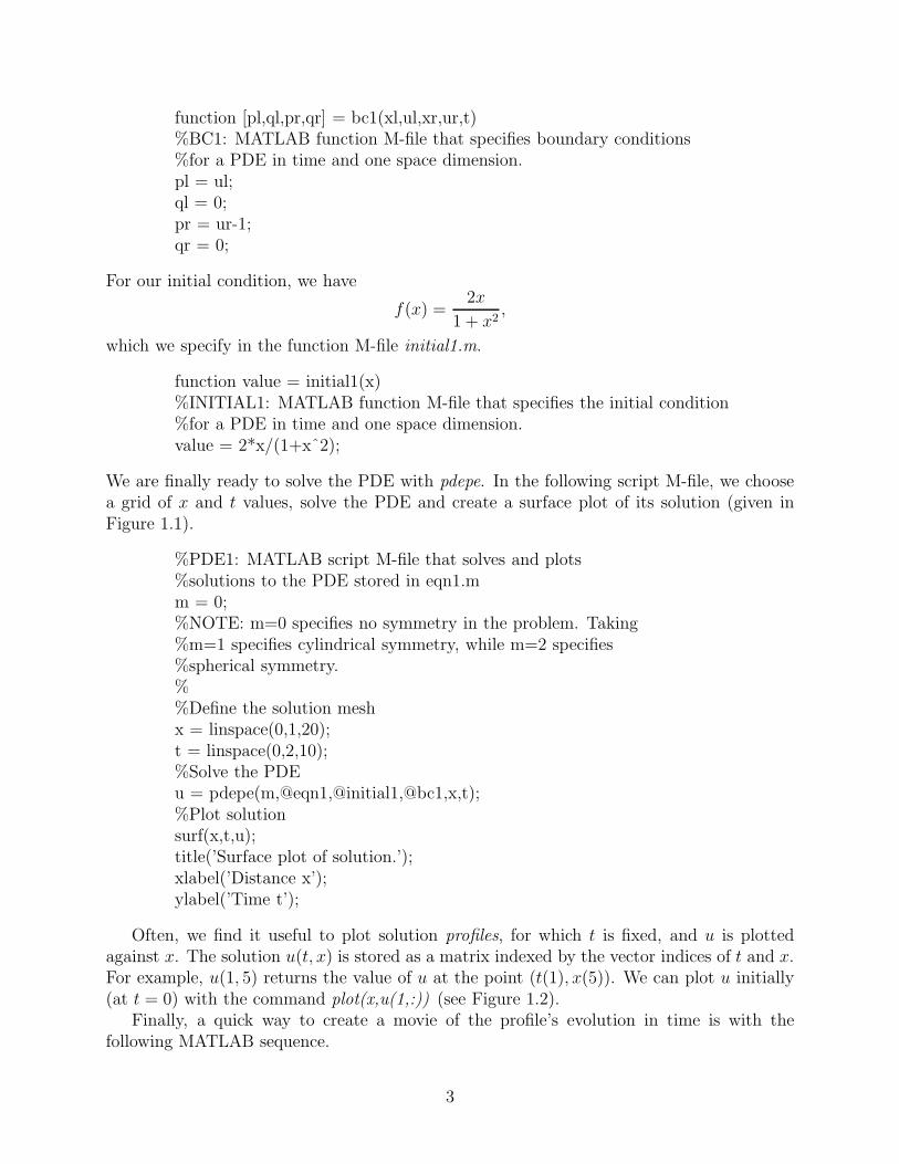
We are finally ready to solve the PDE with pdepe. In the following script M-file, we choosea grid of x and t values, solve the PDE and create a surface plot of its solution (given inFigure 1.1).

%PDE1: MATLAB script M-file that solves and plots%solutions to the PDE stored in eqn1.mm = 0;%NOTE: m=0 specifies no symmetry in the problem. Taking%m=1 specifies cylindrical symmetry, while m=2 specifies%spherical symmetry.%%Define the solution meshx = linspace(0,1,20);t = linspace(0,2,10);%Solve the PDEu = pdepe(m,@eqn1,@initial1,@bc1,x,t);%Plot solutionsurf(x,t,u);title(’Surface plot of solution.’);xlabel(’Distance x’);ylabel(’Time t’);

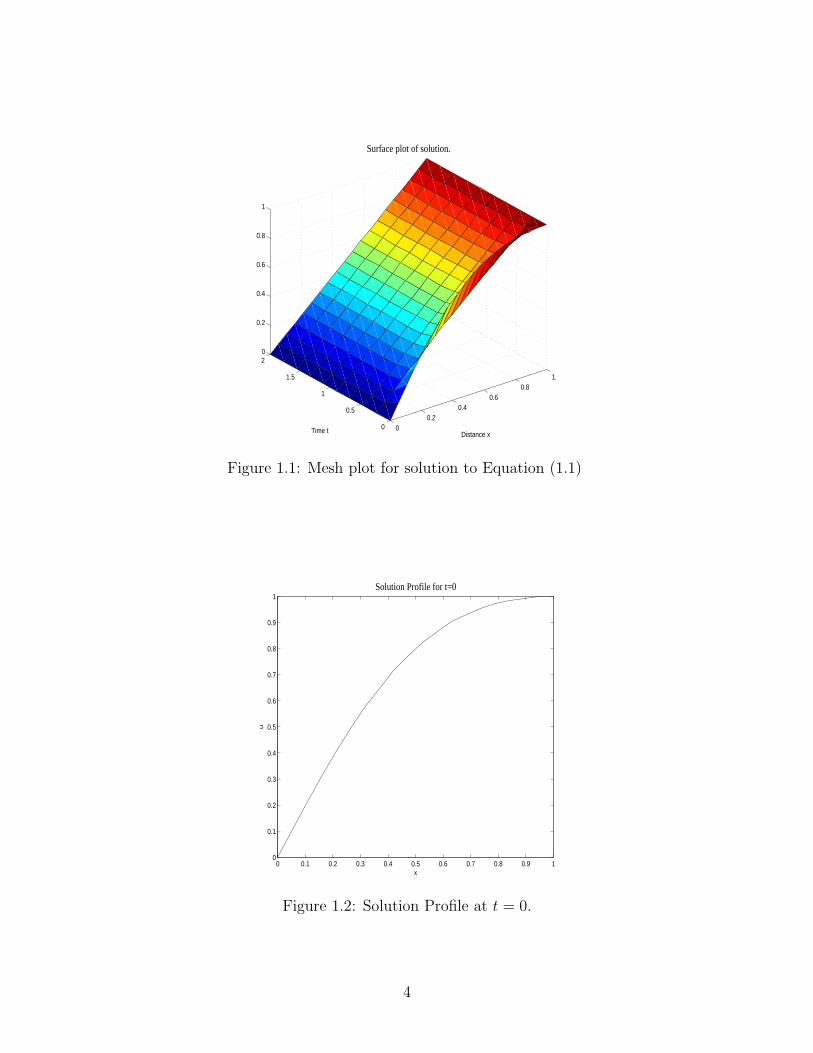
Often, we find it useful to plot solution profiles, for which t is fixed, and u is plottedagainst x. The solution u(t, x) is stored as a matrix indexed by the vector indices of t and x.For example, u(1, 5) returns the value of u at the point (t(1), x(5)). We can plot u initially(at t = 0) with the command plot(x,u(1,:)) (see Figure 1.2).

Finally, a quick way to create a movie of the profile’s evolution in time is with thefollowing MATLAB sequence.

3

00.2

0.40.6

0.81

0

0.5

1

1.5

20

0.2

0.4

0.6

0.8

1

Distance x

Surface plot of solution.

Time t

Figure 1.1: Mesh plot for solution to Equation (1.1)

0 0.1 0.2 0.3 0.4 0.5 0.6 0.7 0.8 0.9 10

0.1

0.2

0.3

0.4

0.5

0.6

0.7

0.8

0.9

1Solution Profile for t=0

x

u

Figure 1.2: Solution Profile at t = 0.

4

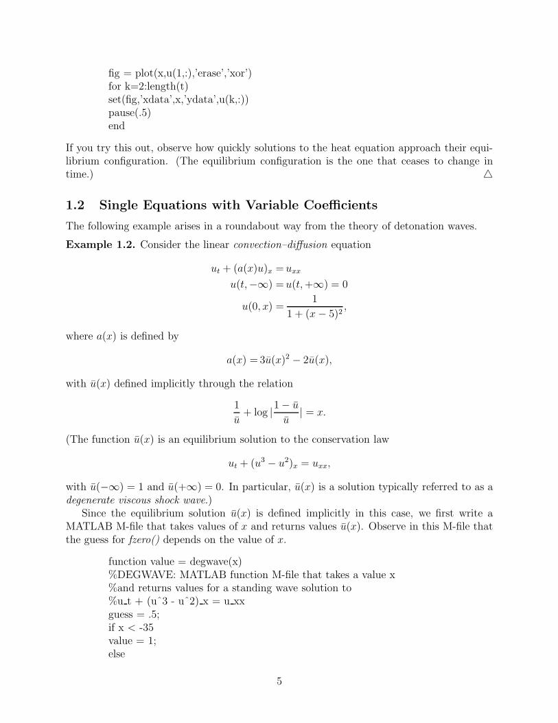
fig = plot(x,u(1,:),’erase’,’xor’)for k=2:length(t)set(fig,’xdata’,x,’ydata’,u(k,:))pause(.5)end

If you try this out, observe how quickly solutions to the heat equation approach their equi-librium configuration. (The equilibrium configuration is the one that ceases to change intime.)

1.2 Single Equations with Variable Coefficients

The following example arises in a roundabout way from the theory of detonation waves.

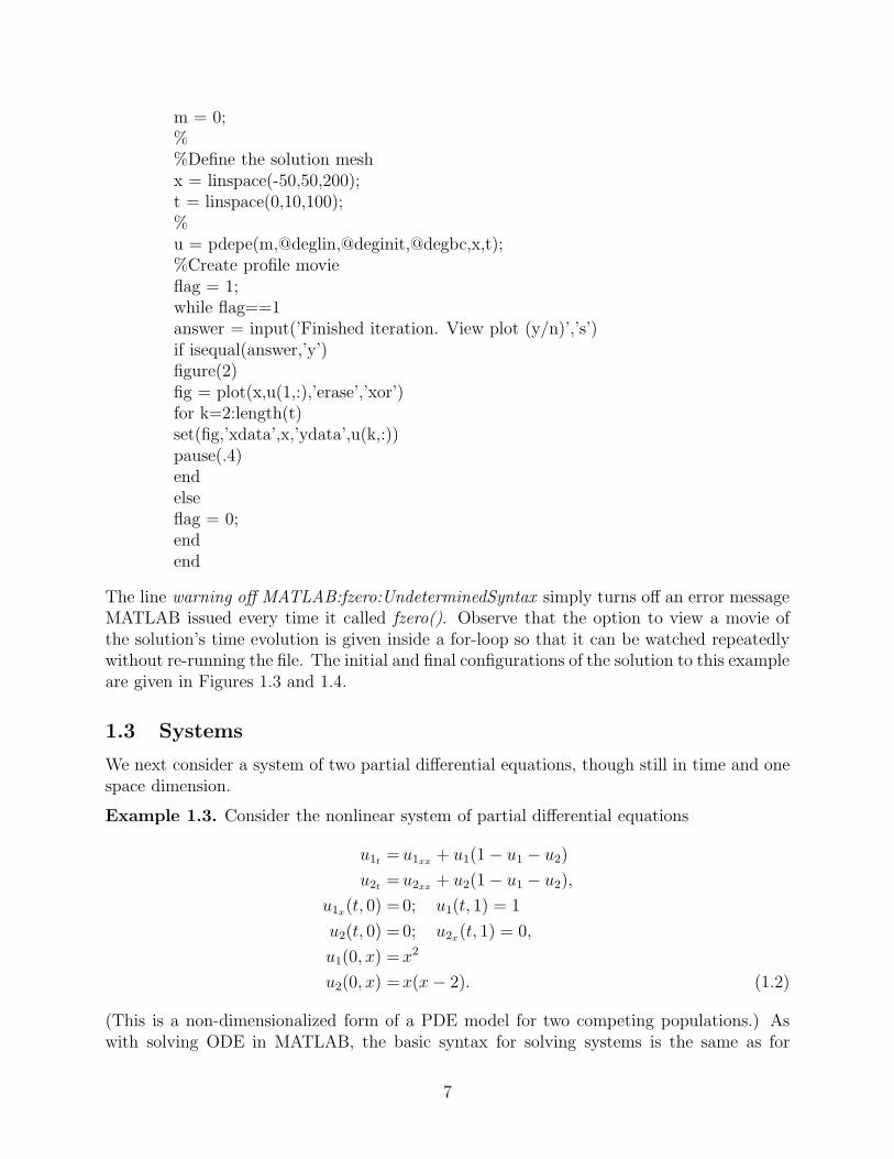
Example 1.2. Consider the linear convection–diffusion equation

ut + (a(x)u)x = uxx

u(t,−∞) = u(t, +∞) = 0

u(0, x) =1

1 + (x − 5)2,

where a(x) is defined by

a(x) = 3u(x)2 − 2u(x),

with u(x) defined implicitly through the relation

1

u+ log |

1 − u

u| = x.

(The function u(x) is an equilibrium solution to the conservation law

ut + (u3 − u2)x = uxx,

with u(−∞) = 1 and u(+∞) = 0. In particular, u(x) is a solution typically referred to as adegenerate viscous shock wave.)

Since the equilibrium solution u(x) is defined implicitly in this case, we first write aMATLAB M-file that takes values of x and returns values u(x). Observe in this M-file thatthe guess for fzero() depends on the value of x.

function value = degwave(x)%DEGWAVE: MATLAB function M-file that takes a value x%and returns values for a standing wave solution to%u t + (uˆ3 - uˆ2) x = u xxguess = .5;if x < -35value = 1;else

5

if x > 2guess = 1/x;elseif x>-2.5guess = .6;elseguess = 1-exp(-2)*exp(x);endvalue = fzero(@f,guess,[],x);endfunction value1 = f(u,x)value1 = (1/u)+log((1-u)/u)-x;

The equation is now stored in deglin.m.

function [c,b,s] = deglin(x,t,u,DuDx)%EQN1: MATLAB function M-file that specifies%a PDE in time and one space dimension.c = 1;b = DuDx - (3*degwave(x)ˆ2 - 2*degwave(x))*u;s = 0;

In this case, the boundary conditions are at ±∞. Since MATLAB only understands finitedomains, we will approximate these conditions by setting u(t,−50) = u(t, 50) = 0. Observethat at least initially this is a good approximation since u0(−50) = 3.2e − 4 and u0(+50) =4.7e − 4. The boundary conditions are stored in the MATLAB M-file degbc.m.

function [pl,ql,pr,qr] = degbc(xl,ul,xr,ur,t)%BC1: MATLAB function M-file that specifies boundary conditions%for a PDE in time and one space dimension.pl = ul;ql = 0;pr = ur;qr = 0;

The initial condition is specified in deginit.m.

function value = deginit(x)%DEGINIT: MATLAB function M-file that specifies the initial condition%for a PDE in time and one space dimension.value = 1/(1+(x-5)ˆ2);

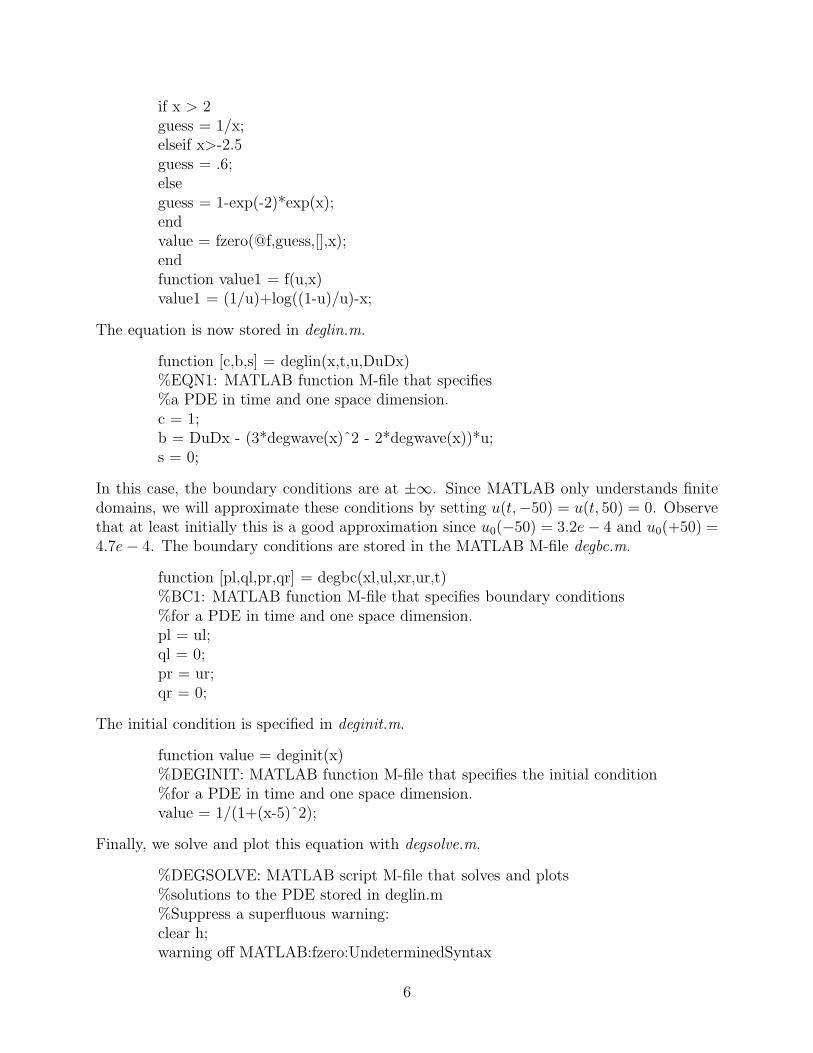
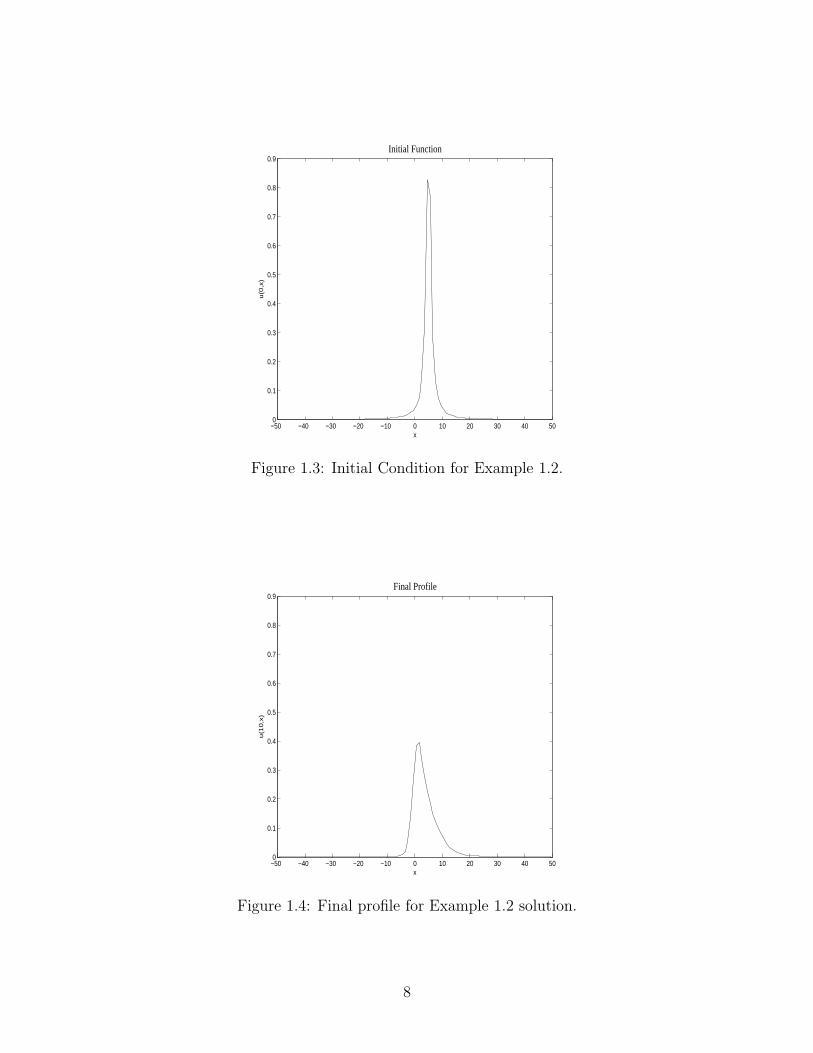
Finally, we solve and plot this equation with degsolve.m.

%DEGSOLVE: MATLAB script M-file that solves and plots%solutions to the PDE stored in deglin.m%Suppress a superfluous warning:clear h;warning off MATLAB:fzero:UndeterminedSyntax

6

m = 0;%%Define the solution meshx = linspace(-50,50,200);t = linspace(0,10,100);%u = pdepe(m,@deglin,@deginit,@degbc,x,t);%Create profile movieflag = 1;while flag==1answer = input(’Finished iteration. View plot (y/n)’,’s’)if isequal(answer,’y’)figure(2)fig = plot(x,u(1,:),’erase’,’xor’)for k=2:length(t)set(fig,’xdata’,x,’ydata’,u(k,:))pause(.4)endelseflag = 0;endend

The line warning off MATLAB:fzero:UndeterminedSyntax simply turns off an error messageMATLAB issued every time it called fzero(). Observe that the option to view a movie ofthe solution’s time evolution is given inside a for-loop so that it can be watched repeatedlywithout re-running the file. The initial and final configurations of the solution to this exampleare given in Figures 1.3 and 1.4.

1.3 Systems

We next consider a system of two partial differential equations, though still in time and onespace dimension.

Example 1.3. Consider the nonlinear system of partial differential equations

u1t=u1xx

+ u1(1 − u1 − u2)

u2t=u2xx

+ u2(1 − u1 − u2),

u1x(t, 0) =0; u1(t, 1) = 1

u2(t, 0) =0; u2x(t, 1) = 0,

u1(0, x) =x2

u2(0, x) =x(x − 2). (1.2)

(This is a non-dimensionalized form of a PDE model for two competing populations.) Aswith solving ODE in MATLAB, the basic syntax for solving systems is the same as for

7

−50 −40 −30 −20 −10 0 10 20 30 40 500

0.1

0.2

0.3

0.4

0.5

0.6

0.7

0.8

0.9Initial Function

x

u(0

,x)

Figure 1.3: Initial Condition for Example 1.2.

−50 −40 −30 −20 −10 0 10 20 30 40 500

0.1

0.2

0.3

0.4

0.5

0.6

0.7

0.8

0.9Final Profile

x

u(1

0,x

)

Figure 1.4: Final profile for Example 1.2 solution.

8

solving single equations, where each scalar is simply replaced by an analogous vector. Inparticular, MATLAB specifies a system of n PDE as

c1(x, t, u, ux)u1t=x−m ∂

∂x

(

xmb1(x, t, u, ux))

+ s1(x, t, u, ux)

c2(x, t, u, ux)u2t=x−m ∂

∂x

(

xmb2(x, t, u, ux))

+ s2(x, t, u, ux)

...

cn(x, t, u, ux)unt=x−m ∂

∂x

(

xmbn(x, t, u, ux))

+ sn(x, t, u, ux),

(observe that the functions ck, bk, and sk can depend on all components of u and ux) withboundary conditions

p1(xl, t, u) + q1(xl, t) · b1(xl, t, u, ux) =0

p1(xr, t, u) + q1(xr, t) · b1(xr, t, u, ux) =0

p2(xl, t, u) + q2(xl, t) · b2(xl, t, u, ux) =0

p2(xr, t, u) + q2(xr, t) · b2(xr, t, u, ux) =0

...

pn(xl, t, u) + qn(xl, t) · bn(xl, t, u, ux) =0

pn(xr, t, u) + qn(xr, t) · bn(xr, t, u, ux) =0,

and initial conditions

u1(0, x) =f1(x)

u2(0, x) =f2(x)

...

un(0, x) =fn(x).

In our example equation, we have

c =

(

c1

c2

)

=

(

11

)

; b =

(

b1

b2

)

=

(

u1x

u2x

)

; s =

(

s1

s2

)

=

(

u1(1 − u1 − u2)u2(1 − u1 − u2)

)

,

which we specify with the MATLAB M-file eqn2.m.

function [c,b,s] = eqn2(x,t,u,DuDx)%EQN2: MATLAB M-file that contains the coefficents for%a system of two PDE in time and one space dimension.c = [1; 1];b = [1; 1] .* DuDx;s = [u(1)*(1-u(1)-u(2)); u(2)*(1-u(1)-u(2))];

9

For our boundary conditions, we have

p(0, t, u) =

(

p1

p2

)

=

(

0u2

)

; q(0, t) =

(

q1

q2

)

=

(

10

)

p(1, t, u) =

(

p1

p2

)

=

(

u1 − 10

)

; q(1, t) =

(

q1

q2

)

=

(

01

)

which we specify in the function M-file bc2.m.

function [pl,ql,pr,qr] = bc2(xl,ul,xr,ur,t)%BC2: MATLAB function M-file that defines boundary conditions%for a system of two PDE in time and one space dimension.pl = [0; ul(2)];ql = [1; 0];pr = [ur(1)-1; 0];qr = [0; 1];

For our initial conditions, we have

u1(0, x) =x2

u2(0, x) =x(x − 2),

which we specify in the function M-file initial2.m.

function value = initial2(x);%INITIAL2: MATLAB function M-file that defines initial conditions%for a system of two PDE in time and one space variable.value = [xˆ2; x*(x-2)];

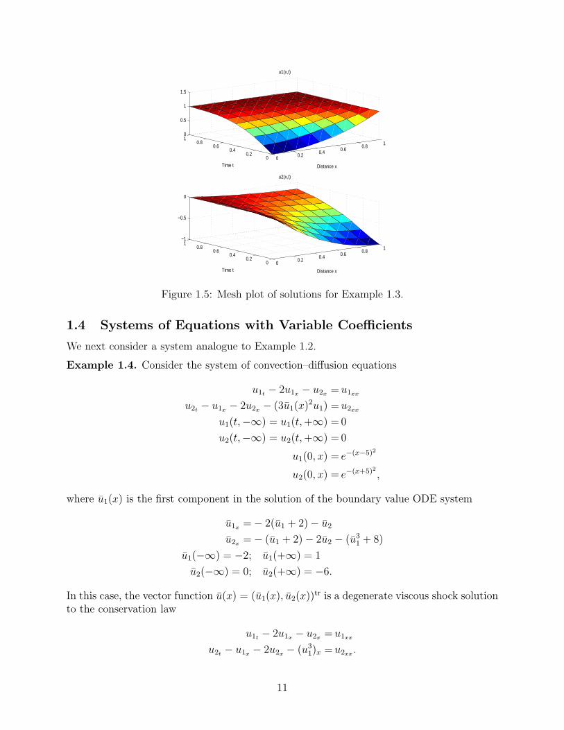
We solve equation (1.2) and plot its solutions with pde2.m (see Figure 1.5).

%PDE2: MATLAB script M-file that solves the PDE%stored in eqn2.m, bc2.m, and initial2.mm = 0;x = linspace(0,1,10);t = linspace(0,1,10);sol = pdepe(m,@eqn2,@initial2,@bc2,x,t);u1 = sol(:,:,1);u2 = sol(:,:,2);subplot(2,1,1)surf(x,t,u1);title(’u1(x,t)’);xlabel(’Distance x’);ylabel(’Time t’);subplot(2,1,2)surf(x,t,u2);title(’u2(x,t)’);xlabel(’Distance x’);ylabel(’Time t’);

10

00.2 0.4 0.6 0.8

1

00.2

0.40.6

0.810

0.5

1

1.5

Distance x

u1(x,t)

Time t

00.2 0.4 0.6 0.8

1

00.2

0.40.6

0.81

−1

−0.5

0

Distance x

u2(x,t)

Time t

Figure 1.5: Mesh plot of solutions for Example 1.3.

1.4 Systems of Equations with Variable Coefficients

We next consider a system analogue to Example 1.2.

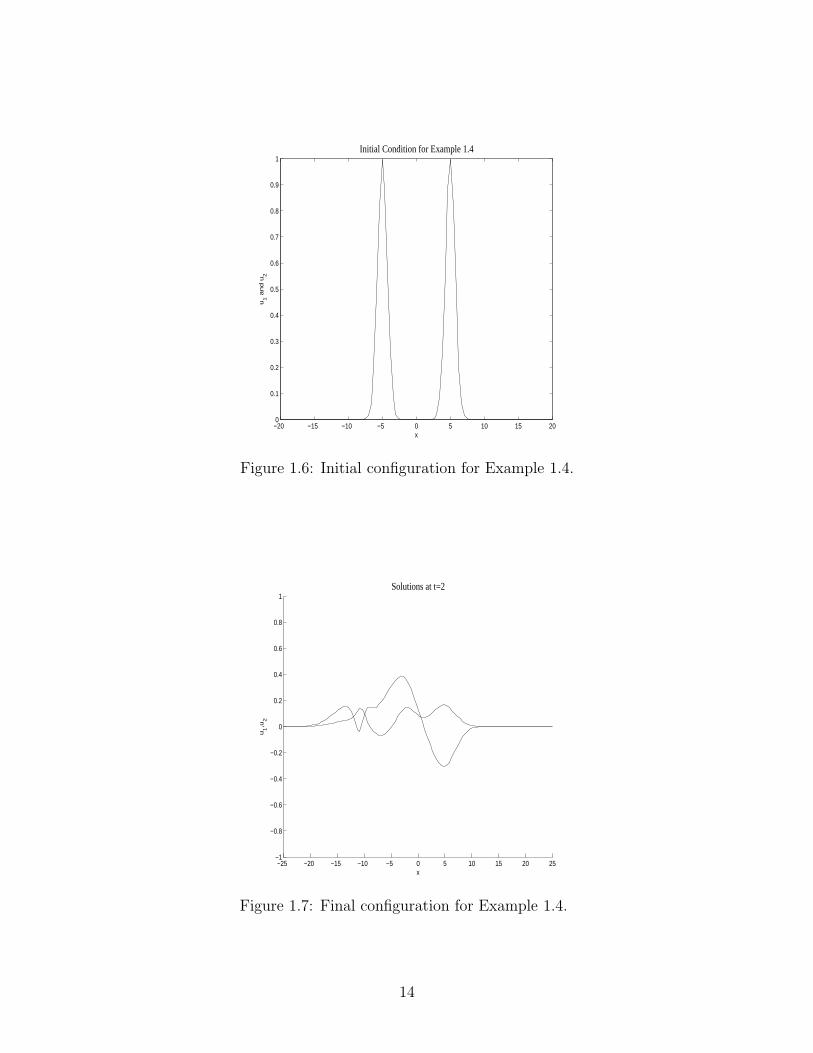
Example 1.4. Consider the system of convection–diffusion equations

u1t− 2u1x

− u2x= u1xx

u2t− u1x

− 2u2x− (3u1(x)2u1) = u2xx

u1(t,−∞) = u1(t, +∞) = 0

u2(t,−∞) = u2(t, +∞) = 0

u1(0, x) = e−(x−5)2

u2(0, x) = e−(x+5)2 ,

where u1(x) is the first component in the solution of the boundary value ODE system

u1x= − 2(u1 + 2) − u2

u2x= − (u1 + 2) − 2u2 − (u3

1 + 8)

u1(−∞) = −2; u1(+∞) = 1

u2(−∞) = 0; u2(+∞) = −6.

In this case, the vector function u(x) = (u1(x), u2(x))tr is a degenerate viscous shock solutionto the conservation law

u1t− 2u1x

− u2x= u1xx

u2t− u1x

− 2u2x− (u3

1)x = u2xx.

11

One of the main obstacles of this example is that it is prohibitively difficult to develop evenan implicit representation for u(x). We will proceed by solving the ODE for u(x) at eachstep in our PDE solution process. First, the ODE for u(x) is stored in degode.m.

function xprime = degode(t,x);%DEGODE: Stores an ode for a standing wave%solution to the p-system.xprime=[-2*(x(1)+2)-x(2); -(x(1)+2)-2*x(2)-(x(1)ˆ3+8)];

We next compute u1(x) in pdegwave.m by solving this ODE with appropriate approximateboundary conditions.

function u1bar=pdegwave(x)%PDEGWAVE: Function M-file that takes input x and returns%the vector value of a degenerate wave.%in degode.msmall = .000001;if x <= -20u1bar = -2;u2bar = 0;elsetspan = [-20 x];%Introduce small perturbation from initial pointx0 = [-2+small,-small];[t,x]=ode45(’degode’,tspan,x0);u1bar = x(end,1);u2bar = x(end,2);end

In this case, we solve the ODE by giving it boundary conditions extremely close to theasymptotic boundary conditions. The critical issue here is that the asymptotic boundaryconditions are equilibrium points for the ODE, so if we started right at the boundary con-dition we would never leave it. We define our boundary conditions and initial conditions inpsysbc.m and degsysinit.m respectively.

function [pl,ql,pr,qr]=psysbc(xl,ul,xr,ur,t)%PSYSBC: Boundary conditions for the linearized%p-system.pl=[ul(1);ul(2)];ql=[0;0];pr=[ur(1);ur(2)];qr=[0;0];

and

function value = degsysinit(x);%DEGSYSINIT: Contains initial condition for linearized%p-system.value = [exp(-(x-5)ˆ2);exp(-(x+5)ˆ2)];

12

The PDE is stored in deglinsys.m.

function [c,b,s] = deglinsys(x,t,u,DuDx)%DEGLINSYS: MATLAB M-file that contains the coefficents for%a system of two PDE in time and one space dimension.c = [1; 1];b = [1; 1] .* DuDx + [2*u(1)+u(2);u(1)+2*u(2)+3*pdegwave(x)ˆ2*u(1)];s = [0;0];

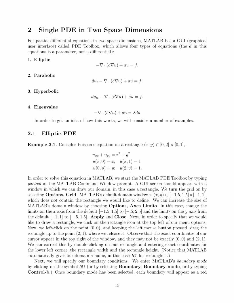
Finally, we solve the PDE and plot its solutions with degsolve.m.

%DEGSOLVE: MATLAB script M-file that solves the PDE%stored in deglinsys.m, psysbc.m, and degsysinit.mclf;m = 0;x = linspace(-25,25,100);t = linspace(0,2,20);sol = pdepe(m,@deglinsys,@degsysinit,@psysbc,x,t);u1 = sol(:,:,1);u2 = sol(:,:,2);flag = 1;while flag==1answer = input(’Finished iteration. View plot (y/n)’,’s’)if isequal(answer,’y’)figure;hold on;fig1=plot(x,u1(1,:),’erase’,’xor’)axis([min(x) max(x) -1 1]);fig2=plot(x,u2(2,:),’r’,’erase’,’xor’)for k=2:length(t)set(fig1,’ydata’,u1(k,:));set(fig2,’ydata’,u2(k,:));pause(.5)endelseflag=0endend

The initial condition for this problem is given in Figure 1.6, while the final configuration isgiven in Figure 1.7. Ideally, this would have been run for a longer time period, but since anODE was solved at each step of the PDE solution process, the compuation was extremelytime-consuming. Evolving the system for two seconds took roughly ten minutes.

13

−20 −15 −10 −5 0 5 10 15 200

0.1

0.2

0.3

0.4

0.5

0.6

0.7

0.8

0.9

1Initial Condition for Example 1.4

x

u1 a

nd

u2

Figure 1.6: Initial configuration for Example 1.4.

−25 −20 −15 −10 −5 0 5 10 15 20 25−1

−0.8

−0.6

−0.4

−0.2

0

0.2

0.4

0.6

0.8

1Solutions at t=2

x

u1,u

2

Figure 1.7: Final configuration for Example 1.4.

14

2 Single PDE in Two Space Dimensions

For partial differential equations in two space dimensions, MATLAB has a GUI (graphicaluser interface) called PDE Toolbox, which allows four types of equations (the d in thisequations is a parameter, not a differential):

1. Elliptic−∇ · (c∇u) + au = f.

2. Parabolicdut −∇ · (c∇u) + au = f.

3. Hyperbolicdutt −∇ · (c∇u) + au = f.

4. Eigenvalue−∇ · (c∇u) + au = λdu

In order to get an idea of how this works, we will consider a number of examples.

2.1 Elliptic PDE

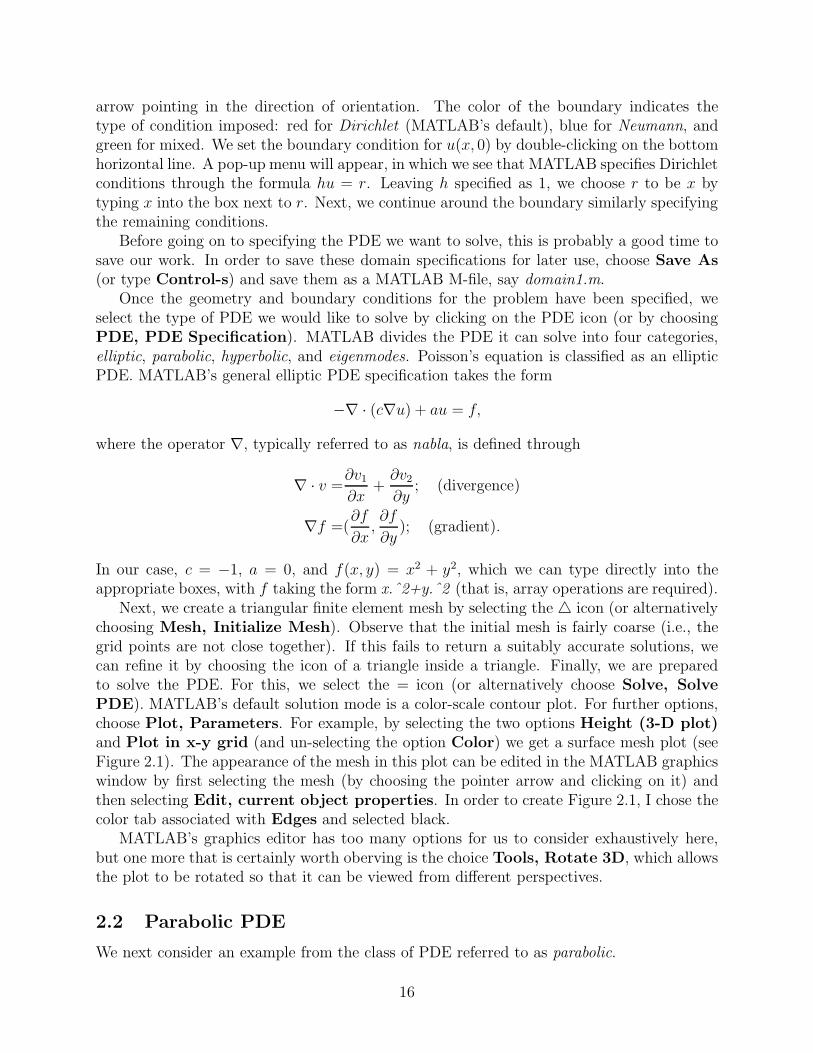
Example 2.1. Consider Poisson’s equation on a rectangle (x, y) ∈ [0, 2] × [0, 1],

uxx + uyy =x2 + y2

u(x, 0) = x; u(x, 1) = 1

u(0, y) = y; u(2, y) = 1.

In order to solve this equation in MATLAB, we start the MATLAB PDE Toolbox by typingpdetool at the MATLAB Command Window prompt. A GUI screen should appear, with awindow in which we can draw our domain, in this case a rectangle. We turn the grid on byselecting Options, Grid. MATLAB’s default domain window is (x, y) ∈ [−1.5, 1.5]×[−1, 1],which does not contain the rectangle we would like to define. We can increase the size ofMATLAB’s domain window by choosing Options, Axes Limits. In this case, change thelimits on the x axis from the default [−1.5, 1.5] to [−.5, 2.5] and the limits on the y axis fromthe default [−1, 1] to [−.5, 1.5]. Apply and Close. Next, in order to specify that we wouldlike to draw a rectangle, we click on the rectangle icon at the top left of our menu options.Now, we left-click on the point (0, 0), and keeping the left mouse button pressed, drag therectangle up to the point (2, 1), where we release it. Observe that the exact coordinates of ourcursor appear in the top right of the window, and they may not be exactly (0, 0) and (2, 1).We can correct this by double-clicking on our rectangle and entering exact coordinates forthe lower left corner, the rectangle width and the rectangle height. (Notice that MATLABautomatically gives our domain a name, in this case R1 for rectangle 1.)

Next, we will specify our boundary conditions. We enter MATLAB’s boundary modeby clicking on the symbol ∂Ω (or by selecting Boundary, Boundary mode, or by typingControl-b.) Once boundary mode has been selected, each boundary will appear as a red

15

arrow pointing in the direction of orientation. The color of the boundary indicates thetype of condition imposed: red for Dirichlet (MATLAB’s default), blue for Neumann, andgreen for mixed. We set the boundary condition for u(x, 0) by double-clicking on the bottomhorizontal line. A pop-up menu will appear, in which we see that MATLAB specifies Dirichletconditions through the formula hu = r. Leaving h specified as 1, we choose r to be x bytyping x into the box next to r. Next, we continue around the boundary similarly specifyingthe remaining conditions.

Before going on to specifying the PDE we want to solve, this is probably a good time tosave our work. In order to save these domain specifications for later use, choose Save As(or type Control-s) and save them as a MATLAB M-file, say domain1.m.

Once the geometry and boundary conditions for the problem have been specified, weselect the type of PDE we would like to solve by clicking on the PDE icon (or by choosingPDE, PDE Specification). MATLAB divides the PDE it can solve into four categories,elliptic, parabolic, hyperbolic, and eigenmodes. Poisson’s equation is classified as an ellipticPDE. MATLAB’s general elliptic PDE specification takes the form

−∇ · (c∇u) + au = f,

where the operator ∇, typically referred to as nabla, is defined through

∇ · v =∂v1

∂x+

∂v2

∂y; (divergence)

∇f =(∂f

∂x,∂f

∂y); (gradient).

In our case, c = −1, a = 0, and f(x, y) = x2 + y2, which we can type directly into theappropriate boxes, with f taking the form x.ˆ2+y.ˆ2 (that is, array operations are required).

Next, we create a triangular finite element mesh by selecting the icon (or alternativelychoosing Mesh, Initialize Mesh). Observe that the initial mesh is fairly coarse (i.e., thegrid points are not close together). If this fails to return a suitably accurate solutions, wecan refine it by choosing the icon of a triangle inside a triangle. Finally, we are preparedto solve the PDE. For this, we select the = icon (or alternatively choose Solve, SolvePDE). MATLAB’s default solution mode is a color-scale contour plot. For further options,choose Plot, Parameters. For example, by selecting the two options Height (3-D plot)and Plot in x-y grid (and un-selecting the option Color) we get a surface mesh plot (seeFigure 2.1). The appearance of the mesh in this plot can be edited in the MATLAB graphicswindow by first selecting the mesh (by choosing the pointer arrow and clicking on it) andthen selecting Edit, current object properties. In order to create Figure 2.1, I chose thecolor tab associated with Edges and selected black.

MATLAB’s graphics editor has too many options for us to consider exhaustively here,but one more that is certainly worth oberving is the choice Tools, Rotate 3D, which allowsthe plot to be rotated so that it can be viewed from different perspectives.

2.2 Parabolic PDE

We next consider an example from the class of PDE referred to as parabolic.

16

0

0.5

1

1.5

2

0

0.2

0.4

0.6

0.8

10

1

2

Height: u

Figure 2.1: Mesh plot for solution to Poission’s equation from Example 2.1.

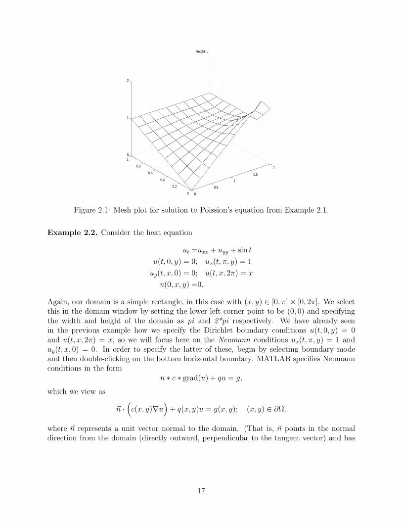
Example 2.2. Consider the heat equation

ut =uxx + uyy + sin t

u(t, 0, y) = 0; ux(t, π, y) = 1

uy(t, x, 0) = 0; u(t, x, 2π) = x

u(0, x, y) =0.

Again, our domain is a simple rectangle, in this case with (x, y) ∈ [0, π] × [0, 2π]. We selectthis in the domain window by setting the lower left corner point to be (0, 0) and specifyingthe width and height of the domain as pi and 2*pi respectively. We have already seenin the previous example how we specify the Dirichlet boundary conditions u(t, 0, y) = 0and u(t, x, 2π) = x, so we will focus here on the Neumann conditions ux(t, π, y) = 1 anduy(t, x, 0) = 0. In order to specify the latter of these, begin by selecting boundary modeand then double-clicking on the bottom horizontal boundary. MATLAB specifies Neumannconditions in the form

n ∗ c ∗ grad(u) + qu = g,

which we view as

~n ·(

c(x, y)∇u)

+ q(x, y)u = g(x, y); (x, y) ∈ ∂Ω,

where ~n represents a unit vector normal to the domain. (That is, ~n points in the normaldirection from the domain (directly outward, perpendicular to the tangent vector) and has

17

unit length.) For the case uy(t, x, 0) = 0, we have

~n =(0,−1) (keep in mind: ~n · ∇u = (n1, n2) · (ux, uy) = n1ux + n2uy)

c(x, 0) =1

q(x, 0) =0

g(x, 0) =0,

of which we specify q and g. (The value of c must correspond with the value of c that ariseswhen we specify our PDE, so we will define it there, keeping in mind that it must be 1.)Similarly, we specify the boundary condition ux(t, π, y) = 1 by setting q = 0 and g = 1.(Observe that our segments of boundary with Dirichlet conditions are shaded red while oursegments of boundary with Neumann conditions are shaded blue.)

We now specify our PDE as in Example 2.1, except this time we choose the optionParabolic. MATLAB specifies parabolic PDE in the form

d ∗ u′ − div(c ∗ grad(u)) + a ∗ u = f,

which we view as

d(t, x, y)ut −∇ · (c(t, x, y)∇u) + a(t, x, y)u = f(t, x, y).

In our case d(t, x, y) = 1, c(t, x, y) = 1, and f(t, x, y) = sin t, which we can type directly intothe pop-up menu. (Write sin t as sin(t).)

Next, we set our initial condition and our times for solution by choosing Solve, Pa-rameters. A vector of times for which we want solution values is specified under Time:and the initial condition is specified under u(t0). A good way to specify time is with thelinspace command, so we type linspace(0,5,10), which runs time from 0 to five seconds, withten points. In this case, we can leave the initial condition specified as 0.

Finally, we introduce a mesh by clicking the icon and then solve with =. (If we select= prior to specifying a mesh, MATLAB will automatically specify a mesh for us.) As before,MATLAB returns a color scale solution, this time at the final time of solution, t = 5. Inorder to get an idea of the time evolution of the solutions, we select Plot, Parameters andchoose Animation. For example, we can set Height (3-D plot), Animation, and Plotin x-y grid, which will produce an evolving mesh plot.

Final remark. In this example, we have specified c as a constant scalar. It can also bespecified as a non-constant scalar or, more generally, as a 2 × 2 non-constant matrix.

3 Linear systems in two space dimensions

We next consider the case of solving linear systems of PDE in time and two space variables.

3.1 Two Equations

Linear systems consisting of two equations can still be solved directly in PDE Toolbox.

18

Example 3.1. Consider the following system of two linear parabolic equations defined ona circle centered at the origin with radius 1 (denoted Ω).

u1t+ (1/(1 + x2))u1 + u2 = u1xx

+ u1yy

u2t+ u1 + u2 = u1xx

+ u2yy

u1(t, x, y) = e−(x2+y2), x < 0, (x, y) ∈ ∂Ω

u2(t, x, y) = sin(x + y), x < 0, (x, y) ∈ ∂Ω

~n · ∇~u = 0, x > 0

u1(0, x, y) = e−(x2+y2)

u2(0, x, y) = sin(x + y).

We begin solving these equations by typing pdecirc(0,0,1) in the MATLAB command win-dow. (The usage of pdecirc is pdecirc(xcenter,ycenter,radius,label), where the label can beomitted.) This will open the MATLAB Toolbox GUI and create a circle centered at theorgin with radius 1. The first thing we need to choose in this case is Options, Applica-tion, Generic System. Next, enter boundary mode and observe that MATLAB expectsboundary conditions for a system of two equations. (That’s what it considers a generic sys-tem. For systems of higher order, we will have to work a little harder.) MATLAB specifiesDirichlet boundary conditions in such systems in the form

(

h11 h12

h21 h22

) (

u1

u2

)

=

(

r1

r2

)

.

Define the two Dirichlet boundary conditions by choosing h11 = h22 = 1 and h12 = h21 = 0(which should be MATLAB’s default values), and by choosing r1 to be exp(-x.ˆ2-y.ˆ2) (don’tomit the array operations) and r2 to be sin(x+y). MATLAB specifies Neumann boundaryconditions in such systems in the form

~n · (c ⊗∇~u) + q~u = g,

where

~n =

(

n1

n2

)

, c =

(

c11 c12

c21 c22

)

, q =

(

q11 q12

q21 q22

)

, and g =

(

g1

g2

)

,

and the kth component of c ⊗∇~u is defined by

c ⊗∇~uk =

(

c11ukx+ c12uky

c21ukx+ c22uky

)

,

so that

~n · (c ⊗∇~u) =

(

n1c11u1x+ n1c12u1y

+ n2c21u1x+ n2c22u1y

n1c11u2x+ n1c12u2y

+ n2c21u2x+ n2c22u2y

)

.

(More generally, if the diffusion isn’t the same for each variable, c can be defined as a tensor,see below.) In this case, taking q and g both zero suffices. (The matrix c will be defined inthe problem as constant, identity.)

19

Next, specify the PDE as parabolic. For parabolic systems, MATLAB’s specificationtakes the form

dut −∇ · (c ⊗∇u) + au = f,

where

u =

(

u1

u2

)

, f =

(

f1

f2

)

, a =

(

a11 a12

a21 a22

)

, d =

(

d11 d12

d21 d22

)

,

and

∇ · (c ⊗∇u) =

(

c11u1xx+ c12u1yx

+ c21u1xy+ c22u1yy

c11u2xx+ c12u1yx

+ c21u1xy+ c22u1yy

)

.

In this case, we take c11 = c22 = 1 and c12 = c21 = 0. Also, we have

(

a11 a12

a21 a22

)

=

(

11+x2 1

1 1

)

,

(

d11 d12

d21 d22

)

=

(

1 00 1

)

, and

(

f1

f2

)

=

(

00

)

,

which can all be specified by typing valid MATLAB expressions into the appropriate textboxes. (For the expression 1

1+x2 , we must use array operations, 1./(1+x.ˆ2).)We specify the initial conditions by selecting Solve, Parameters. In this case, we set

the time increments to be linspace(0,10,25), and we specify the vector initial values in u(t0)as [exp(-x.ˆ2-y.ˆ2);sin(x+y)]. Finally, solve the problem by selecting the = icon. (MATLABwill create a mesh automatically.)

The first solution MATLAB will plot is a color plot of u1(x, y), which MATLAB refersto as u. In order to view a similar plot of u2, choose Plot, Parameters and select theProperty v.

4 Nonlinear elliptic PDE in two space dimensions

Though PDE Toolbox is not generally equipped for solving nonlinear problems directly, inthe case of elliptic equations certain nonlinearities can be accomodated.

4.1 Single nonlinear elliptic equations

Example 4.1. Consider the nonlinear elliptic PDE in two space dimensions, defined on theball of radius 1,

u + u(1 − ux − uy) =2u2

u(x, y) = 1;∀(x, y) ∈ ∂B(0, 1).

We begin solving this equation in MATLAB by typing pdecirc(0,0,1) at the MATLABprompt. Proceeding as in the previous examples, we set the boundary condition to beDirichlet and identically 1, and then choose PDE Specification and specify the PDE asElliptic. In this case, we must specify c as 1.0, a as -(1-ux-uy) and f as -2u.ˆ2. The keypoint to observe here is that nonlinear terms can be expressed in terms of u, ux, and uy,for which MATLAB uses respectively u, ux, and uy. Also, we observe that array operations

20

must be used in the expressions. Next, in order to solve the nonlinear problem, we mustchoose Solve, Parameters and specify that we want to use MATLAB’s nonlinear solver. Inthis case, the default nonlinear tolerance of 1e-4 and the designation of Jacobian as Fixedare sufficient, and we are ready to solve the PDE by selecting the icon =.

5 General nonlinear systems in two space dimensions

5.1 Parabolic Problems

While MATLAB’s PDE Toolbox does not have an option for solving nonlinear parabolicPDE, we can make use of its tools to develop short M-files that will solve such equations.

Example 5.1. Consider the Lotka–Volterra predator–prey model in two space dimensions,

u1t= c11u1xx

+ c12u1yy+ a1u1 − r1u1u2

u2t= c21u2xx

+ c22u2xx− a2u2 + r2u1u2,

where u1(t, x, y) represents prey population density at time t and position (x, y) and u2(t, x, y)represents predator population density at time t and position (x, y). For a1, r1, a2, and r2,we will take values obtained from an ODE model for the Hudson Bay Company Hare–Lynxexample: a1 = .47, r1 = .024, a2 = .76, and r2 = .023. For the values ckj, we takec11 = c12 = .1 and c21 = c22 = .01, which signifies that the prey diffuse through the domainfaster than the predators. MATLAB’s PDE Toolbox does not have an option for solving anequation of this type, so we will proceed through an iteration of the form

un+11t

− c11un+11xx

− c12un+11yy

− a1un+11 = − r1u

n1u

n2

un+12t

− c21un+12xx

− c22un+12yy

+ a2un+12 =r2u

n1u

n2 . (5.1)

That is, given u1 and u2 at some time t0 (beginning with the initial conditions), we solvethe linear parabolic equation over a short period of time to determine values of u1 and u2 attime t1.

In general, initial and boundary conditions can be difficult to pin down for problems likethis, but for this example we will assume that the domain is square of length 1 (denoted S),that neither predator nor prey enters or exits the domain, and that initially the predatordensity is concentrated at the edges of the domain and the prey density is concentrated atthe center. In particular, we will assume the following:

~n · ∇u1 =0, ∀x ∈ ∂S

~n · ∇u2 =0, ∀x ∈ ∂S

u1(0, x, y) =

10, (x − 12)2 + (y − 1

2)2 ≤ 1

16

0, otherwise

u2(0, x, y) =

10, (x − 12)2 + (y − 1

2)2 ≥ 1

4

0, otherwise.

21

Though we will have to carry out the actual calculation with an M-file, we will first createthe domain and define our boundary conditions using PDE Toolbox. To begin, at theMATLAB command line prompt, type pderect([0 1 0 1]), which will initiate a session withPDE Toolbox and define a square of length one with lower left corner at the origin. (Theexact usage of pderect is pderect([xmin xmax ymin ymax])). Since the upper edge of thissquare is on the edge of our window, choose Options, Axes Equal, which will expand they axis to the interval [−1.5, 1.5]. Next, choose boundary mode, and then hold the Shift keydown while clicking one after the other on each of the borders. When they are all selected,click on any one of them and set the boundary condition to be Neumann with g and q both0. Once the boundary conditions are set, export them by selecting Boundary, ExportDecomposed Boundary. The default boundary value assignments are g (for geometry)and b (for boundary). For clarity, rename these g1 and b1 to indicate that these are theboundary conditions for u1. (Though for this problem the boundary conditions for u1 andu2 are the same, for generality’s sake, we will treat them as if they were different.) For u2,export the boundary again and this time label as g2 and b2. The last thing we can do in theGUI window is create and export our triangulation, so select the icon to create a meshand select Mesh, Export Mesh to export it. The three variables associated with the meshare p, e, and t, vectors containing respectively the points if the triangulation, the edges ofthe triangulation, and an index of the triangulation.

At this point it’s a good idea to save these variables as a MATLAB workspace (.matfile). To do this, choose File, Save Workspace As. Finally, we store the initial conditionsu1(0, x, y) and u2(0, x, y) in the function M-file lvinitial.m.

function [u1initial,u2initial] = lvinitial(x,y)%LVINITIAL: MATLAB function M-file that contains the%initial population distributions for the Lotka-Volterra model.if (x-1/2)ˆ2+(y-1/2)ˆ2<=1/16u1initial=10;elseu1initial=0;endif (x-1/2)ˆ2+(y-1/2)ˆ2<=1/4u2initial=0;elseu2initial=10;end

Now, we can solve the PDE with the MATLAB M-file lvpde.m. While this file might lookprohibitively lengthy, it’s actually fairly simple. For example, the long sections in bold typesimply plot the solution and can be ignored with regard to understanding how the M-fileworks.

%LVPDE: MATLAB script M-file for solving the PDE%Lotka-Volterra system.%%Parameter definitions

22

a1=.47; r1=.024; a2=.76; r2=.023;m=size(p,2); %Number of endpointsn=size(t,2); %Number of trianglest final=1.0; %Stop timeM=30; %Take 30 time stepsdt=t final/M; %Time-stepping increment (M-file time-stepping)tlist=linspace(0,dt,2); %Time vector for MATLAB’s time-stepping%Rectangular coordinates for plottingx=linspace(0,1,25);y=linspace(0,1,25);%Set diffusionc1=.1; %Prey diffusionc2=.01; %Predator diffusion%Initial conditionsfor i=1:m %For each point of the triangular grid[u1old(i),u2old(i)]=lvinitial(p(1,i),p(2,i));end%for k=1:M%Nonlinear interactionfor i=1:mf1(i)=-r1*u1old(i)*u2old(i);f2(i)=r2*u1old(i)*u2old(i);end%NOTE: The nonlinear interaction terms must be defined at the centerpoints%of the triangles. We can accomplish this with the function%pdeintrp (pde interpolate).f1center=pdeintrp(p,t,f1’);f2center=pdeintrp(p,t,f2’);%Solve the PDEu1new=parabolic(u1old,tlist,b1,p,e,t,c1,-a1,f1center,1);u2new=parabolic(u2old,tlist,b2,p,e,t,c2,a2,f2center,1);%Update u1old, u2oldu1old=u1new(:,2);u2old=u2new(:,2);%Plot each iterationu1=tri2grid(p,t,u1old,x,y);u2=tri2grid(p,t,u2old,x,y);subplot(2,1,1)%imagesc(x,y,u1,[0 10])%colorbarmesh(x,y,u1)axis([0 1 0 1 0 10])subplot(2,1,2)%imagesc(x,y,u2, [0 10])

23

%colorbarmesh(x,y,u2)axis([0 1 0 1 0 10])pause(.1)%end

In general, the function

parabolic(u0,tlist,b,p,e,t,c,a,f,d)

solves the the single PDEdut −∇ · (c∇u) + au = f.

or the system of PDEsdut −∇ · (c ⊗∇u) + au = f.

In this case, according to (5.1), we take the nonlinearity as a driving term from the previoustime step, and the remaining linear equations are decoupled, so that we solve two singleequations rather than a system.

A critical parameter in the development above is M , which determines how refined ourtime-stepping will be (the larger M is, the more refined our analysis is). We can heuristicallycheck our numerical solution by increasing the value of M and checking if the solution remainsconstant.

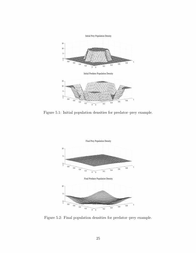
The plotting code creates a window in which mesh plots of both the predator and preypopulation densities are plotted. These are updated at each iteration, so running this code,we see a slow movie of the progression. Example plots of the initial and final populationdensities are given in Figures 5.1 and 5.2. Another good way to view the solution is througha color pixel plot, created by the command imagesc. If we comment out the mesh and axiscommands above and add the imagesc and colorbar commands instead, we can take a bird’seye view of a color-coded depiction of the dynamics.

In lvpde.m the diffusion is taken to have the simple form

.1u1xx+ .1u1yy

.01u2xx+ .01u2yy

.

In order to understand how this can be generalized, we observe that the generic MATLABform

dut −∇ · (c∇u) + au = f,

expands asdut − c11uxx − c12uxy − c21uyx − c22uyy + au = f.

Note carefully that the matrix

c =

(

c11 c12

c21 c22

)

24

00.2 0.4 0.6 0.8

1

00.2

0.40.6

0.810

5

10

15

Initial Prey Population Density

00.2 0.4 0.6 0.8

1

00.2

0.40.6

0.810

5

10

15

Initial Predator Population Density

Figure 5.1: Initial population densities for predator–prey example.

00.2 0.4 0.6 0.8

1

00.2

0.40.6

0.810

5

10

Final Prey Population Density

00.2 0.4 0.6 0.8

1

00.2

0.40.6

0.810

5

10

Final Predator Population Density

Figure 5.2: Final population densities for predator–prey example.

25

does not contain the values cij in our Lotka–Volterra example. In particular, MATLAB usesthis full matrix to specify a single equation. If c is specifed as a single constant (as c1 andc2 are in lvpde.m), then MATLAB takes

c =

(

c 00 c

)

,

giving the form for our example. On the other hand, if c is specified as a column vector withtwo components c = [c1; c2] then MATLAB takes

c =

(

c1 00 c2

)

.

Finally—and this is perhaps a bit peculiar—if c is specified as a column vector with fourcomponents c = [c11; c21; c12; c22] (not as a matrix; note the order) then MATLAB takes

c =

(

c11 c12

c21 c22

)

.

As an example, suppose that in our Lotka-Volterra example we would like to specify thediffusion as

.1u1xx+ .4u + .3u1yy

.01u2xx+ .04u2xy

+ .03u2yy.

We would specify

c1 = [.1; .2; .2; .3]

c2 = [.01; .02; .02; .03].

6 Defining more complicated geometries

One of the biggest advantages in using the GUI interface of MATLAB’s PDE toolbox is theease with which fairly complicated geometries can be defined and triangularized.

7 FEMLAB

7.1 About FEMLAB

FEMLAB is a program developed by COMSOL Ltd. for solving PDE numerically based onthe finite element method. COMSOL Ltd. is the same group who developed MATLAB’sPDE Toolbox, and consequently the GUI for FEMLAB is conveniently similar to the GUIfor PDE Toolbox. The difference between the two programs is that FEMLAB is considerablymore general. Some fundamental features that FEMLAB offers and PDE Toolbox does notare:

26

1. The ability to solve PDE in three space dimensions

2. The ability to solve several additional predefined equations, including

(a) Navier–Stokes

(b) Reaction–convection–diffusion equations

(c) Maxwell’s equations for electrodynamics

3. The ability to solve nonlinear systems of equations directly from the GUI interface.

7.2 Getting Started with FEMLAB

FEMLAB is such a broad program that it’s easy on first glance to get lost in the options.Though our eventual goal in using FEMLAB is to solve fairly complicated equations thatPDE Toolbox is not equipped for, we will begin, as we did with PDE Toolbox, with a simpleexample.

Example 7.1. Consider Poisson’s equation on the ball of radius 1,

u =u(1 − u), (x, y) ∈ B(0, 1)

u(x, y) =x3 + y3, (x, y) ∈ ∂B(0, 1).

We open FEMLAB at the MATLAB Command Window prompt by typing femlab. A ge-ometry window should open with a pop-up menu labeled Model Navigator. We observeimmediately that FEMLAB offers the choice of one, two, or three dimensions. We choose2D (which should be the default) and then double-click on Classical PDEs. FEMLAB’soptions under Classical PDEs are:

• Laplace’s equation

• Poisson’s equation

• Helmholtz’s equation

• Heat equation

• Wave equation

• Schrodinger equation

• Convection–diffusion equation

We can select the option Poisson’s equation by double-clicking on it, after which weobserve that Poisson’s Equation appears in the upper left corner of the FEMLAB geometrywindow. In this case, the default grid in the geometry window is too small, so we increaseit by selecting Options, Axes/Grid Settings and specifying a y range between -1.5 and1.5. We can now draw a circle of radius 1 by selecting the ellipse icon from the left panel ofthe window, clicking on the point (0, 0) and dragging the radius to 1. By default, FEMLAB

27

labels this region E1 for ellipse 1. As in PDE Toolbox, we can double-click anywhere inthe region to alter or refine its definition. Next, we choose Boundary, Boundary modeand specify our boundary condition by selecting each part of the curve and choosing theDirichlet boundary conditions with h as 1 and r as x.ˆ3+y.ˆ3. (For the moment, we willdo well to ignore the options for more complicated boundary value selections.) Next, weneed to specify our governing equation. FEMLAB is set up so that different equations canbe specified in different regions of the domain, so equation specification is made under theoption Subdomain, Subdomain Settings. FEMLAB specifies Poisson’s equation in theform

−∇ · (c∇u) = f,

so in this case we choose c to be 1 and f to be -u.*(1-u). Finally, we solve the PDE byselecting Solve, Solve Problem. We observe that FEMLAB offers a number of options forviewing the solutions, listed as icons on the left corner of the geometry window.

28

Index

Dirichlet boundary condition, 16

elliptic PDE, 15

imagesc(), 24

Neumann boundary condition, 16

parabolic(), 24PDE Toolbox, 15pdecirc(), 19pdepe(), 1pderect(), 22pdetool, 15Poisson’s equation, 15

29