partial least squares structural equation modelingpartial least squares structural equation modeling...

Partial Least Squares Structural EquationModeling

Marko Sarstedt, Christian M. Ringle, and Joseph F. Hair

AbstractPartial least squares structural equation modeling (PLS-SEM) has become apopular method for estimating (complex) path models with latent variables andtheir relationships. Building on an introduction of the fundamentals of measure-ment and structural theory, this chapter explains how to specify and estimate pathmodels using PLS-SEM. Complementing the introduction of the PLS-SEMmethod and the description of how to evaluate analysis results, the chapter alsooffers an overview of complementary analytical techniques. An application of thePLS-SEM method to a well-known corporate reputation model using theSmartPLS 3 software illustrates the concepts.

KeywordsPartial least squares • PLS • PLS path modeling PLS-SEM • SEM • Variance-based structural equation modeling

M. Sarstedt (*)Otto-von-Guericke University, Magdeburg, Germany

Faculty of Business and Law, University of Newcastle, Callaghan, NSW, Australiae-mail: [email protected]

C.M. RingleHamburg University of Technology (TUHH), Hamburg, Germany

Faculty of Business and Law, University of Newcastle, Callaghan, NSW, Australiae-mail: [email protected]

J.F. HairUniversity of South Alabama, Mobile, AL, USAe-mail: [email protected]

# Springer International Publishing AG 2017C. Homburg et al. (eds), Handbook of Market Research,https://doi.org/10.1007/978-3-319-05542-8_15-1

mailto:[email protected]



https://doi.org/10.1007/978-3-319-05542-8_15-1

ContentsIntroduction . . . . . . . . . . . . . . . . . . . . . . . . . . . . . . . . . . . . . . . . . . . . . . . . . . . . . . . . . . . . . . . . . . . . . . . . . . . . . . . . . . . . . . . 2Principles of Structural Equation Modeling . . . . . . . . . . . . . . . . . . . . . . . . . . . . . . . . . . . . . . . . . . . . . . . . . . . . . . 3

Path Models with Latent Variables . . . . . . . . . . . . . . . . . . . . . . . . . . . . . . . . . . . . . . . . . . . . . . . . . . . . . . . . . . . 3Structural Theory . . . . . . . . . . . . . . . . . . . . . . . . . . . . . . . . . . . . . . . . . . . . . . . . . . . . . . . . . . . . . . . . . . . . . . . . . . . . . . 4Measurement Theory . . . . . . . . . . . . . . . . . . . . . . . . . . . . . . . . . . . . . . . . . . . . . . . . . . . . . . . . . . . . . . . . . . . . . . . . . . 5

Path Model Estimation with PLS-SEM . . . . . . . . . . . . . . . . . . . . . . . . . . . . . . . . . . . . . . . . . . . . . . . . . . . . . . . . . . 7Background . . . . . . . . . . . . . . . . . . . . . . . . . . . . . . . . . . . . . . . . . . . . . . . . . . . . . . . . . . . . . . . . . . . . . . . . . . . . . . . . . . . . 7The PLS-SEM Algorithm . . . . . . . . . . . . . . . . . . . . . . . . . . . . . . . . . . . . . . . . . . . . . . . . . . . . . . . . . . . . . . . . . . . . . 8Additional Considerations When Using PLS-SEM . . . . . . . . . . . . . . . . . . . . . . . . . . . . . . . . . . . . . . . . . . 11

Evaluation of PLS-SEM Results . . . . . . . . . . . . . . . . . . . . . . . . . . . . . . . . . . . . . . . . . . . . . . . . . . . . . . . . . . . . . . . . . 14Procedure . . . . . . . . . . . . . . . . . . . . . . . . . . . . . . . . . . . . . . . . . . . . . . . . . . . . . . . . . . . . . . . . . . . . . . . . . . . . . . . . . . . . . . 14Stage 1.1: Reflective Measurement Model Assessment . . . . . . . . . . . . . . . . . . . . . . . . . . . . . . . . . . . . . . 15Stage 1.2: Formative Measurement Model Assessment . . . . . . . . . . . . . . . . . . . . . . . . . . . . . . . . . . . . . 18Stage 2: Structural Model Assessment . . . . . . . . . . . . . . . . . . . . . . . . . . . . . . . . . . . . . . . . . . . . . . . . . . . . . . . 20

Research Application . . . . . . . . . . . . . . . . . . . . . . . . . . . . . . . . . . . . . . . . . . . . . . . . . . . . . . . . . . . . . . . . . . . . . . . . . . . . . 22Corporate Reputation Model . . . . . . . . . . . . . . . . . . . . . . . . . . . . . . . . . . . . . . . . . . . . . . . . . . . . . . . . . . . . . . . . . . 22Data . . . . . . . . . . . . . . . . . . . . . . . . . . . . . . . . . . . . . . . . . . . . . . . . . . . . . . . . . . . . . . . . . . . . . . . . . . . . . . . . . . . . . . . . . . . . 25Model Estimation . . . . . . . . . . . . . . . . . . . . . . . . . . . . . . . . . . . . . . . . . . . . . . . . . . . . . . . . . . . . . . . . . . . . . . . . . . . . . 25Results Evaluation . . . . . . . . . . . . . . . . . . . . . . . . . . . . . . . . . . . . . . . . . . . . . . . . . . . . . . . . . . . . . . . . . . . . . . . . . . . . 26

Conclusions . . . . . . . . . . . . . . . . . . . . . . . . . . . . . . . . . . . . . . . . . . . . . . . . . . . . . . . . . . . . . . . . . . . . . . . . . . . . . . . . . . . . . . . 32Cross-References . . . . . . . . . . . . . . . . . . . . . . . . . . . . . . . . . . . . . . . . . . . . . . . . . . . . . . . . . . . . . . . . . . . . . . . . . . . . . . . . . 33References . . . . . . . . . . . . . . . . . . . . . . . . . . . . . . . . . . . . . . . . . . . . . . . . . . . . . . . . . . . . . . . . . . . . . . . . . . . . . . . . . . . . . . . . 34

Introduction

In the 1970s and 1980s the Swedish econometrician Herman O. A. Wold (1975,1982, 1985) “vigorously pursued the creation and construction of models andmethods for the social sciences, where ‘soft models and soft data’ were the rulerather than the exception, and where approaches strongly oriented at predictionwould be of great value” (Dijkstra 2010, p. 24). One procedure that emerged fromWold’s efforts was partial least squares path modeling, which later evolved to partialleast squares structural equation modeling (PLS-SEM; Hair et al. 2011). PLS-SEMestimates the parameters of a set of equations in a structural equation model bycombining principal components analysis with regression-based path analysis(Mateos-Aparicio 2011). Wold (1982) proposed his “soft model basic design”underlying PLS-SEM as an alternative to Jöreskog’s (1973) factor-based SEM orcovariance-based SEM, which has been labeled as hard modeling because of itsnumerous and rather restrictive assumptions for establishing a structural equationmodel but also in terms of data distribution and sample size. Importantly, “it is notthe concepts nor the models nor the estimation techniques which are ‘soft’, only thedistributional assumptions” (Lohmöller 1989, p. 64).

PLS-SEM enjoys widespread popularity in a broad range of disciplines includingaccounting (Lee et al. 2011; Nitzl 2016), group and organization management (Sosiket al. 2009), hospitality management (Ali et al. 2017), international management(Richter et al. 2016a), operations management (Peng and Lai 2012), managementinformation systems (Hair et al. 2017a; Ringle et al. 2012), marketing (Hair et al.

2 M. Sarstedt et al.

2012b), strategic management (Hair et al. 2012a), supply chain management(Kaufmann and Gaeckler 2015), and tourism (do Valle and Assaker 2016). Contri-butions in terms of books, edited volumes, and journal articles applying PLS-SEM orproposing methodological extensions are appearing at a rapid pace (e.g., Latan andNoonan 2017; Esposito Vinzi et al. 2010; Hair et al. 2017b, 2018; Garson 2016;Ramayah et al. 2016). A main reason for PLS-SEM’s attractiveness is that themethod allows researchers to estimate very complex models with many constructsand indicator variables, especially when prediction is the goal of the analysis.Furthermore, PLS-SEM generally allows for much flexibility in terms of datarequirements and the specification of relationships between constructs and indicatorvariables. Another reason is the accessibility of easy to use software with graphicaluser interface such as ADANCO, PLS-Graph, SmartPLS, WarpPLS, and XLSTAT.Packages for statistical computing software environments such as R complement theset of programs (e.g., semPLS).

The objective of this chapter is to explain the fundamentals of PLS-SEM.Building on Sarstedt et al. (2016b), this chapter first provides an introduction ofmeasurement and structural theory as a basis for presenting the PLS-SEM method.Next, the chapter discusses the evaluation of results, provides an overview ofcomplementary analytical techniques, and concludes by describing an applicationof the PLS-SEM method to a well-known corporate reputation model, using theSmartPLS 3 software.

Principles of Structural Equation Modeling

Path Models with Latent Variables

A path model is a diagram that displays the hypotheses and variable relationships tobe estimated in an SEM analysis (Bollen 2002). Figure 1 shows an example of a pathmodel with latent variables and their indicators.

Constructs, also referred to as latent variables, are elements in statistical modelsthat represent conceptual variables that researchers define in their theoretical models.Constructs are visualized as circles or ovals (Y1 to Y3) in path models, linked viasingle-headed arrows that represent predictive relationships. The indicators, oftenalso named manifest variables or items, are directly measured or observed variablesthat represent the raw data (e.g., respondents’ answers to a questionnaire). Theyare represented as rectangles (x1 to x9) in path models and are linked to theircorresponding constructs through arrows.

A path model consists of two elements. The structural model represents thestructural paths between the constructs, whereas the measurement models representthe relationships between each construct and its associated indicators. In PLS-SEM,structural and measurement models are also referred to as inner and outer models. Todevelop path models, researchers need to draw on structural theory and measurementtheory, which specify the relationships between the elements of a path model.

Partial Least Squares Structural Equation Modeling 3

Structural Theory

Structural theory indicates the latent variables to be considered in the analysis ofa certain phenomenon and their relationships. The location and sequence of theconstructs are based on theory and the researcher’s experience and accumulatedknowledge (Falk and Miller 1992). When researchers develop path models, thesequence is typically from left to right. The latent variables on the left side of thepath model are independent variables, and any latent variable on the right side isthe dependent variable (Fig. 1). However, latent variables may also serve as both anindependent and dependent variable in the model (Haenlein and Kaplan 2004).

When a latent variable only serves as an independent variable, it is called anexogenous latent variable (Y1 in Fig. 1). When a latent variable only serves as adependent variable (Y3 in Fig. 1), or as both an independent and a dependent variable(Y2 in Fig. 1), it is called an endogenous latent variable. Endogenous latent variablesalways have error terms associated with them. In Fig. 1, the endogenous latentvariables Y2 and Y3 have one error term each (z2 and z3), which reflect the sourcesof variance not captured by the respective antecedent construct(s) in the structuralmodel. The exogenous latent variable Y1 also has an error term (z1) but in PLS-SEM,this error term is constrained to zero because of the way the method treats the(formative) measurement model of this particular construct (Diamantopoulos2011). Therefore, this error term is typically omitted in the display of a PLS pathmodel. In case an exogenous latent variable draws on a reflective measurementmodel, there is no error term attached to this particular construct.

The strength of the relationships between latent variables is represented by pathcoefficients (i.e., b1, b2, and b3), and the coefficients are the result of regressions ofeach endogenous latent variable on their direct predecessor constructs. For example,b1 and b3 result from the regression of Y3 on Y1 and Y2.

Y1

Y2

Y3

l7

x2

x3

x1

x5

x6

x4 x9

x8

x7 e7

z3

e4

e5

e6

z2

b1

b2

b3

w1

z1

w2

w3

l5

l4

l6

l8l9

e8

e9

Fig. 1 Path model with latent variables


Measurement Theory

The measurement theory specifies how to measure latent variables. Researcherscan generally choose between two different types of measurement models(Diamantopoulos and Winklhofer 2001; Coltman et al. 2008): reflective measure-ment models and formative measurement models.

Reflective measurement models have direct relationships from the construct tothe indicators and treat the indicators as error-prone manifestations of the underlyingconstruct (Bollen 1989). The following equation formally illustrates the relationshipbetween a latent variable and its observed indicators:

x ¼ lY þ e (1)

where x is the observed indicator variable, Y is the latent variable, the loading l is aregression coefficient quantifying the strength of the relationship between x and Y,and e represents the random measurement error. The latent variables Y2 and Y3 in thepath model shown in Fig. 1 have reflective measurement models with three indica-tors each. When using reflective indicators (also called effect indicators), the itemsshould be a representative sample of all items of the construct’s conceptual domain(Nunnally and Bernstein 1994). If the items stem from the same domain, theycapture the same concept and, hence, should be highly correlated (Edwards andBagozzi 2000).

In contrast, in a formative measurement model, a linear combination of a set ofindicators forms the construct (i.e., the relationship is from the indicators to theconstruct). Hence, “variation in the indicators precedes variation in the latentvariable” (Borsboom et al. 2003, p. 2008). Indicators of formatively measuredconstructs do not necessarily have to correlate strongly as is the case with reflectiveindicators. Note that strong indicator correlations can also occur in formativemeasurement models and do not necessarily imply that the measurement model isreflective in nature (Nitzl and Chin 2017).

When referring to formative measurement models, researchers need to distinguishtwo types of indicators: causal indicators and composite indicators (Bollen 2011;Bollen and Bauldry 2011). Constructs measured with causal indicators have an errorterm, which implies that the construct has not been perfectly measured by itsindicators (Bollen and Bauldry 2011). More precisely, causal indicators show con-ceptual unity in that they correspond to the researcher’s definition of the concept(Bollen and Diamantopoulos 2017), but researchers will hardly ever be able toidentify all indicators relevant for adequately capturing the construct’s domain (e.g., Bollen and Lennox 1991). The error term captures all the other “causes” orexplanations of the construct that the set of causal indicators do not capture(Diamantopoulos 2006). The existence of a construct error term in causal indicatormodels suggests that the construct can, in principle, be equivalent to the conceptualvariable of interest, provided that the model has perfect fit (e.g., Grace and Bollen2008). In case the indicators x1, x2, and x3 represent causal indicators, Y1’s error term


z1 would capture these other “causes” (Fig. 1). A measurement model with causalindicators can formally be described as

Y ¼XKk¼1

wk � xk þ z, (2)

where wk indicates the contribution of xk (k = 1, . . ., K ) to Y, and z is an error termassociated with Y.

Composite indicators constitute the second type of indicators associated withformative measurement models. When using measurement models with compositeindicators, researchers assume that the indicators define the construct in full (Sarstedtet al. 2016b). Hence, the error term, which in causal indicator models represents“omitted causes,” is set to zero in formative measurement models with compositeindicators (z1 = 0 in Fig. 1). Hence, a measurement model with composite indicatorstakes the following form, where Y is a linear combination of indicators xk (k= 1, . . .,K ), each weighted by an indicator weight wk (Bollen 2011; McDonald 1996):

Y ¼XKk¼1

wk � xk: (3)

According to Henseler (2017, p. 180), measurement models with compositeindicators “are a prescription of how the ingredients should be arranged to form anew entity,” which he refers to as artifacts. That is, composite indicators define theconstruct’s empirical meaning. Henseler (2017) identifies Aaker’s (1991) conceptu-alization of brand equity as a typical conceptual variable with composite indicators (i.e., an artifact) in advertising research, comprising the elements brand awareness,brand associations, brand quality, brand loyalty, and other proprietary assets. Theuse of artifacts is especially prevalent in the analysis of secondary and archival data,which typically lack a comprehensive substantiation on the grounds of measurementtheory (Rigdon 2013a; Houston 2004). For example, a researcher may use secondarydata to form an index of a company’s communication activities, covering aspects suchas online advertising, sponsoring, or product placement (Sarstedt and Mooi 2014).Alternatively, composite indicator models can be thought of as a means to capture theessence of a conceptual variable by means of a limited number of indicators (Dijkstraand Henseler 2011). For example, a researcher may be interested in measuring acompany’s corporate social responsibility using a set of five (composite) indicatorsthat capture salient features relevant to the particular study. More recent researchcontends that composite indicators can be used to measure any concept includingattitudes, perceptions, and behavioral intentions (Nitzl and Chin 2017). However,composite indicators are not a free ride for careless measurement. Instead, “as withany type of measurement conceptualization, however, researchers need to offer a clearconstruct definition and specify items that closely match this definition – that is, theymust share conceptual unity” (Sarstedt et al. 2016b, p. 4002). Composite indicatormodels rather view construct measurement as approximation of conceptual variables,


acknowledging the practical problems that come with measuring unobservable con-ceptual variables that populate theoretical models. Whether researchers deem anapproximation as sufficient depends on their philosophy of science. From an empir-ical realist perspective, researchers want to see results from causal and compositeindicators converging upon the conceptual variable, which they assume exists inde-pendent of observation and transcends data. An empiricist defines a certain concept interms of data, a function of observed variables, leaving the relationship betweenconceptual variable and construct untapped (Rigdon et al. 2017).

Path Model Estimation with PLS-SEM

Background

Different from factor-based SEM, PLS-SEM explicitly calculates case values forthe latent variables as part of the algorithm. For this purpose, the “unobservablevariables are estimated as exact linear combinations of their empirical indicators”(Fornell and Bookstein 1982, p. 441) such that the resulting composites capture mostof the variance of the exogenous constructs’ indicators that is useful for predictingthe endogenous constructs’ indicators (e.g., McDonald 1996). PLS-SEM uses thesecomposites to represent the constructs in a PLS path model, considering them asapproximations of the conceptual variables under consideration (e.g., Henseler et al.2016a; Rigdon 2012).

Since PLS-SEM-based model estimation always relies on composites, regardlessof the measurement model specification, the method can process reflectively andformatively specified measurement models without identification issues (Hair et al.2011). Identification of PLS path models only requires that each construct is linkedwith a significant path to the nomological net of constructs (Henseler et al. 2016a).This characteristic also applies to model settings in which endogenous constructs arespecified formatively as PLS-SEM relies on a multistage estimation process, whichseparates measurement from structural model estimation (Rigdon et al. 2014).

Three aspects are important for understanding the interplay between data, mea-surement, and model estimation in PLS-SEM. First, PLS-SEM handles all indicatorsof formative measurement models as composite indicators. Hence, a formativelyspecified construct in PLS-SEM does not have an error term as is the case with causalindicators in factor-based SEM (Diamantopoulos 2011).

Second, when the data stem from a common factor model population (i.e., theindicator covariances define the data’s nature), PLS-SEM’s parameter estimatesdeviate from the prespecified values. This characteristic, also known as PLS-SEMbias, entails that the method overestimates the measurement model parameters andunderestimates the structural model parameters (e.g., Chin et al. 2003). The degreeof over- and underestimation decreases when both the number of indicators perconstruct and sample size increase (consistency at large; Hui and Wold 1982).However, some recent work on PLS-SEM urges researchers to avoid the termPLS-SEM bias since the characteristic is based on specific assumptions about the


nature of the data that do not necessarily have to hold (e.g., Rigdon 2016). Specif-ically, when the data stem from a composite model population in which linearcombinations of the indicators define the data’s nature, PLS-SEM estimates areunbiased and consistent (Sarstedt et al. 2016b). Apart from that, research hasshown that the bias produced by PLS-SEM when estimating data from commonfactor model populations is low in absolute terms (e.g., Reinartz et al. 2009),particularly when compared to the bias that common factor-based SEM produceswhen estimating data from composite model populations (Sarstedt et al. 2016b).“Clearly, PLS is optimal for estimating composite models while simultaneouslyallowing approximating common factor models with effect indicators with practi-cally no limitations” (Sarstedt et al. 2016b, p. 4008).

Third, PLS-SEM’s use of composites not only has implications for the method’sphilosophy of measurement but also for its area of application. In PLS-SEM, oncethe weights are derived, the method always produces a single specific (i.e., determi-nate) score for each case per composite. Using these scores as input, PLS-SEMapplies a series of ordinary least squares regressions, which estimate the modelparameters such that they maximize the endogenous constructs’ explained variance(i.e., their R2 values). Evermann and Tate’s (2016) simulation studies show that PLS-SEM outperforms factor-based SEM in terms of prediction. In light of their results,the authors conclude that PLS-SEM allows researchers “to work with an explana-tory, theory-based model, to aid in theory development, evaluation, and selection.”Similarly, Becker et al.’s (2013a) simulation study provides support for PLS-SEM’ssuperior predictive capabilities.

The PLS-SEM Algorithm

Model estimation in PLS-SEM draws on a three-stage approach that belongs to thefamily of (alternating) least squares algorithms (Mateos-Aparicio 2011). Figure 2illustrates the PLS-SEM algorithm as presented by Lohmöller (1989). Henseler et al.(2012b) offer a graphical illustration of the SEM algorithm’s stages.

The algorithm starts with an initialization stage in which it establishes preliminarylatent variable scores. To compute these scores, the algorithm typically uses unitweights (i.e., 1) for all indicators in the measurement models (Hair et al. 2017b).

Stage 1 of the PLS-SEM algorithm iteratively determines the inner weights andlatent variable scores by means of a four-step procedure – consistent with the algo-rithm’s original presentation (Lohmöller 1989), inner weights refer to path coefficients,while outer weights and outer loadings refer to indicator weights and loadings in themeasurement models. Step #1 uses the initial latent variable scores from the initiali-zation of the algorithm to determine the inner weights bji between the adjacent latentvariables Yj (i.e., the dependent one) and Yi (i.e., the independent one) in the structuralmodel. The literature suggests three approaches to determine the inner weights(Lohmöller 1989; Chin 1998; Tenenhaus et al. 2005). In the centroid scheme, theinner weights are set toþ1 if the covariance between Yj and Yi is positive and�1 if thiscovariance is negative. In case two latent variables are unconnected, theweight is set to


0. In the factor weighting scheme, the inner weight corresponds to the covariancebetween Yj and Yi and is set to zero in case the latent variables are unconnected. Finally,the path weighting scheme takes into account the direction of the inner model relation-ships (Lohmöller 1989). Chin (1998, p. 309) notes that the path weighting scheme“attempts to produce a component that can both ideally be predicted (as a predictand)and at the same time be a good predictor for subsequent dependent variables.” As aresult, the path weighting scheme leads to slightly higher R2 values in the endogenouslatent variables compared to the other schemes and should therefore be preferred. Inmost instances, however, the choice of the inner weighting scheme has very littlebearing on the results (Noonan and Wold 1982; Lohmöller 1989).

Step #2, the inside approximation, computes proxies for all latent variables ~Yj byusing the weighted sum of its adjacent latent variables scores Yi. Then, for all theindicators in the measurement models, Step #3 computes new outer weights indi-cating the strength of the relationship between each latent variable ~Yj and itscorresponding indicators. To do so, the PLS-SEM algorithm uses two differentestimation modes. When using Mode A (i.e., correlation weights), the bivariatecorrelation between each indicator and the construct determine the outer weights.In contrast, Mode B (i.e., regression weights) computes indicator weights byregressing each construct on its associated indicators.

Initialization

Stage 1: Iterative estimation of weights and latent variable scores

Starting at step #4, repeat steps #1 to #4 until convergence is obtained.

#1 Inner weights (here obtained by using the factor weighting scheme)

#2 Inside approximation

∑= i ijij YbY :~

#3 Outer weights; solve for

blockBModeain~~

block A Modeain~~

nkjnkkjn

jnnkkjn

jj

jk jj

eYwx

dxwY

+=

+= ∑

#4 Outside approximation

∑jk jj nkkjn xwY ~:=

Stage 2: Estimation of outer weights, outer loadings, and path coefficients

Stage 3: Estimation of location parameters

otherwise

are adjacentYandYif)Y;(Yv ijij

ji⎩⎨⎧

0

cov=

Fig. 2 The basic PLS-SEM algorithm (adapted from Lohmöller 1989, p. 29).


By default, estimation of reflectively specified constructs draws on Mode A,whereas PLS-SEM uses Mode B for formatively specified constructs. However,Becker et al. (2013a) show that this reflex-like use of Mode A and Mode B is notoptimal under all conditions. For example, when constructs are specified forma-tively, Mode A estimation yields better out-of-sample prediction when the modelestimation draws on more than 100 observations and when the endogenous con-struct’s R2 value is 0.30 or higher.

Figure 2 shows the formal representation of these two modes, where xkjn representsthe raw data for indicator k (k = 1,. . .,K) of latent variable j ( j = 1,. . .,J) andobservation n (n = 1,. . .,N), ~Yjn are the latent variable scores from the insideapproximation in Step #2, ~wkj are the outer weights from Step #3, djn is the errorterm from a bivariate regression, and ekjn is the error term from a multiple regression.The updated weights from Step #3 (i.e., ~wkj ) and the indicators (i.e., xkjn) are linearlycombined to update the latent variables scores (i.e., Yjn) in Step #4 (outside approxi-mation). Note that the PLS-SEM algorithm uses standardized data as input and alwaysstandardizes the generated latent variable scores in Step #2 and Step #4. After Step #4,a new iteration starts; the algorithm terminates when theweights obtained fromStep #3change marginally from one iteration to the next (typically 1 � 10�7), or when themaximum number of iterations is achieved (typically 300; Henseler 2010).

Stages 2 and 3 use the final latent variable scores from Stage 1 as input for a seriesof ordinary least squares regressions. These regressions produce the final outerloadings, outer weights, and path coefficients as well as related elements such asindirect and total effects, R2 values of the endogenous latent variables, and theindicator and latent variable correlations (Lohmöller 1989).

Research has proposed several variations of the original PLS-SEM algorithm.Lohmöller’s (1989) extended PLS-SEM algorithm, for example, allows assigningmore than one latent variable to a block of indicators and imposing orthogonalityrestrictions among constructs in the structural model.More recently, Becker and Ismail(2016) developed a modified version of the original PLS-SEM algorithm that usessampling (post-stratification) weights to correct for sampling error. Their weightedPLS-SEM approach considers a weights vector defined by the researcher in order toensure correspondence between sample and population structure (Sarstedt et al. 2017).

Moreover, Dijkstra and Henseler (2015a, b) introduced the consistent PLS (PLSc)approach, which has also been generalized to nonlinear structural equation models(Dijkstra and Schermelleh-Engel 2014). PLSc is a modified version of Lohmöller’s(1989) original PLS-SEM algorithm that produces model estimates that follow a com-mon factor model approach to measurement – see Dijkstra and Henseler (2015b) for anempirical comparison of PLSc and factor-based SEM. Note that PLSc’s introduction hasalso been viewed critically, however, because of its focus on common factor models. Asindicated by Hair et al. (2017a, p. 443): “It is unclear why researchers would use thesealternative approaches to PLS-SEMwhen they could easily apply themuchmorewidelyrecognized and validated CB-SEM [i.e., factor-based SEM] method.” PLS-SEM doesnot produce inconsistent estimates per se but only when used to estimate common factormodels, just like factor-based SEM produces inconsistent estimates when used to


estimate composite models (Sarstedt et al. 2016b). In addition to the already existing butinfrequently used capabilities to estimate unstandardized coefficients (with or withoutintercept), Dijkstra and Henseler (2015b) contend that PLS-SEM and PLSc provide abasis for the implementation of other, more versatile estimators of structural modelrelationships, such as two-stage least squares and seemingly unrelated regression.These extensions would facilitate analysis of path models with circular relationshipsbetween the latent variables (so called nonrecursive models).

Further methodological advances may facilitate, for example, the consideration ofendogeneity in the structural model, which occurs when an endogenous latent vari-able’s error term is correlated with the scores of one or more explanatory variables ina partial regression relationship.

Additional Considerations When Using PLS-SEM

Research has witnessed a considerable debate about situations that favor or hinderthe use of PLS-SEM (e.g., Goodhue et al. 2012; Marcoulides et al. 2012; Marcoulidesand Saunders 2006; Rigdon 2014a; Henseler et al. 2014). Complementing our abovediscussion of the method’s treatment of latent variables and the consequences formeasurement model specification and estimation, in the following sections weintroduce further aspects that are relevant when considering using PLS-SEM, andwhich have been discussed in the literature (e.g., Hair et al. 2013). Where necessary,we refer to differences to factor-based SEM even though such comparisons shouldnot be made indiscriminately (e.g., Marcoulides and Chin 2013; Rigdon 2016;Rigdon et al. 2017; Hair et al. 2017c).

Distributional AssumptionsMany researchers indicate that they prefer the nonparametric PLS-SEM approachbecause their data’s distribution does not meet the requirements of the parametricfactor-based SEM approach (e.g., Hair et al. 2012b; Nitzl 2016; do Valle and Assaker2016). Methods researchers have long noted, however, that this sole justification forPLS-SEM use is inappropriate since maximum likelihood estimation in factor-basedSEM is robust against violations of normality (e.g., Chou et al. 1991; Olsson et al.2000). Furthermore, factor-based SEM literature offers robust procedures for param-eter estimation, which work well at smaller sample sizes (Lei and Wu 2012).

Consequently, justifying the use of PLS-SEM solely on the grounds of datadistribution is not sufficient (Rigdon 2016). Researchers should rather choose thePLS-SEM method for more profound reasons (see Richter et al. 2016b) such as thegoal of their analysis.

Statistical PowerWhen using PLS-SEM, researchers benefit from the method’s greater statisticalpower compared to factor-based SEM, even when estimating data generated froma common factor model population. Because of its greater statistical power, the PLS-SEM method is more likely to identify an effect as significant when it is indeed


significant. However, while several studies have offered evidence for PLS-SEM’sincreased statistical power (e.g., Reinartz et al. 2009; Goodhue et al. 2012), also vis-á-vis other composite-based approaches to SEM (Hair et al. 2017c), prior researchhas not examined the origins of this feature.

The characteristic of higher statistical power makes PLS-SEM particularly suit-able for exploratory research settings where theory is less developed and the goal isto reveal substantial (i.e., strong) effects (Chin 2010). As Wold (1980, p. 70) notes,“the arrow scheme is usually tentative since the model construction is an evolution-ary process. The empirical content of the model is extracted from the data, and themodel is improved by interactions through the estimation procedure between themodel and the data and the reactions of the researcher.”

Model Complexity and Sample SizePLS-SEM works efficiently with small sample sizes when models are complex (e.g.,Fornell and Bookstein 1982; Willaby et al. 2015). Prior reviews of SEM use show thatthe average number of constructs per model is clearly higher in PLS-SEM (approx-imately eight constructs; e.g., Kaufmann and Gaeckler 2015; Ringle et al. 2012)compared to factor-based SEM (approximately five constructs; e.g., Shah and Gold-stein 2006; Baumgartner and Homburg 1996). Similarly, the number of indicators perconstruct is typically higher in PLS-SEM compared to factor-based SEM, which is notsurprising considering the negative effect of more indicators on χ2-based fit measuresin factor-based SEM. Different from factor-based SEM, the PLS-SEM algorithm doesnot simultaneously compute all the model relationships (see previous section), butinstead uses separate ordinary least squares regressions to estimate the model’s partialregression relationships – as implied by its name. As a result, the overall number ofmodel parameters can be extremely high in relation to the sample size as long as eachpartial regression relationship draws on a sufficient number of observations. Reinartzet al. (2009), Henseler et al. (2014), and Sarstedt et al. (2016b) show that PLS-SEMprovides solutions when other methods do not converge, or develop inadmissiblesolutions, regardless of whether using common factor or composite model data.However, as Hair et al. (2013, p. 2) note, “some researchers abuse this advantageby relying on extremely small samples relative to the underlying population” and that“PLS-SEM has an erroneous reputation for offering special sampling capabilities thatno other multivariate analysis tool has” (also see Marcoulides et al. 2009).

PLS-SEM can be applied with smaller samples in many instances when othermethods fail, but the legitimacy of such analyses depends on the size and the natureof the population (e.g., in terms of its heterogeneity). No statistical method –including PLS-SEM – can offset a badly designed sample (Sarstedt et al. 2017).To determine the necessary sample size, researchers should run power analyses thattake into account the model structure expected effect sizes and the significance level(e.g. Marcoulides and Chin 2013) and provide power tables for a range of pathmodel constellations. Kock and Hadaya (2017) suggest two new methods fordetermining the minimum sample size in PLS-SEM applications.

While much focus has been devoted to PLS-SEM’s small sample size capabilities(e.g., Goodhue et al. 2012), discussions often ignore that the method is also suitable


for the analysis of large data quantities such as those produced in Internet research,social media, and social network applications (e.g., Akter et al. 2017). Analyses ofsocial media data typically focus on prediction, rely on complex models with littletheoretical substantiation (Stieglitz et al. 2014), and often lack a comprehensivesubstantiation on the grounds of measurement theory (Rigdon 2013b). PLS-SEM’snonparametric nature, its ability to handle complex models with many (e.g., sayeight or considerably more) constructs and indicators along with its high statisticalpower, makes the method a valuable method for social media analytics and theanalysis of other types of large-scale data.

Goodness-of-FitPLS-SEM does not have an established goodness-of-fit measure. As a consequence,some researchers conclude that PLS-SEM’s use for theory testing and confirmation islimited (e.g., Westland 2015). Recent research has, however, started reexamininggoodness-of-fit measures proposed in the early days of PLS-SEM (Lohmöller 1989)or suggesting new ones, thereby broadening the method’s applicability (Henseler et al.2014; Dijkstra and Henseler 2015a). Examples of goodness-of-fit measures suggestedin a PLS-SEM context include standardized root mean square residual (SRMR), theroot mean square residual covariance (RMStheta), the normed fit index (NFI; alsoreferred to as Bentler-Bonett index), the non-normed fit index (NNFI; also referred toas Tucker-Lewis index), and the exact model fit test (Dijkstra and Henseler 2015a;Lohmöller 1989; Henseler et al. 2014). Note that the goodness-of-fit criterion pro-posed by Tenenhaus et al. (2005) does not represent a valid measure of model fit(Henseler and Sarstedt 2013). Also, the use of the NFI usually is not recommended asit systematically improves for more complex models (Hu and Bentler 1998).

Several notes of caution are important regarding the use of goodness-of-fitmeasures in PLS-SEM: First and foremost, literature casts doubt on whether mea-sured fit – as understood in a factor-based SEM context – is a relevant concept forPLS-SEM (Hair et al. 2017b; Rigdon 2012; Lohmöller 1989). Factor-based SEMfollows an explanatory modeling perspective in that the algorithm estimates all themodel parameters such that the divergence between the empirical covariance matrixand the model-implied covariance matrix is minimized. In contrast, the PLS-SEMalgorithm follows a prediction modeling perspective in that the method aims tomaximize the amount of explained variance of the endogenous latent variables.Explanation and prediction are two distinct concepts of statistical modeling andestimation. “In explanatory modeling the focus is on minimizing bias to obtain themost accurate representation of the underlying theory. In contrast, predictive model-ing seeks to minimize the combination of bias and estimation variance, occasionallysacrificing theoretical accuracy for improved empirical precision” (Shmueli 2010, p.293). Correspondingly, a grossly misspecified model can yield superior predictionswhereas a correctly specified model can perform extremely poor in terms of predic-tion – see the Appendix in Shmueli (2010) for an illustration. Researchers usingPLS-SEM overcome this seeming dichotomy between explanatory and predictivemodeling since they expect their model to have high predictive accuracy, while alsobeing grounded in well-developed causal explanations. Gregor (2006, p. 626) refers


to this interplay as explanation and prediction theory, noting that this approach“implies both understanding of underlying causes and prediction, as well as descrip-tion of theoretical constructs and the relationships among them.” This perspectivecorresponds to Jöreskog and Wold’s (1982, p. 270) understanding of PLS-SEM wholabeled the method as a “causal-predictive” technique, meaning that when structuraltheory is strong, path relationships can be interpreted as causal. Hence, validationusing goodness-of-fit measures is also relevant in a PLS-SEM context but less socompared to factor-based SEM. Instead, researchers should primarily rely on criteriathat assess the model’s predictive performance (e.g., Rigdon 2012, 2014b). Forexample, Shmueli et al. (2016) introduced a new approach to assess PLS-SEM’sout-of-sample prediction on the item level, which extends Stone-Geisser’s cross-validation for measuring the predictive relevance of PLS path models (Wold 1982).

Table 1 summarizes the rules of thumb researchers should consider when deter-mining whether PLS-SEM is the appropriate statistical tool for their research.

Evaluation of PLS-SEM Results

Procedure

Evaluating PLS-SEM results involves completing two stages, as illustrated in Fig. 3.Stage 1 addresses the examination of reflective measurement models (Stage 1.1),formative measurement models (Stage 1.2), or both. If the evaluation providessupport for the measurement quality, the researcher continues with the structuralmodel evaluation in Stage 2 (Hair et al. 2017b). In brief, Stage 1 examines themeasurement theory, while Stage 2 covers the structural theory that involves testingthe proposed hypotheses and that addresses the relationships among the latentvariables.

Table 1 Reasons for using PLS-SEM

Reasons for using PLS-SEM

The goal is to predict and explain a key target construct and/or to identify its relevant antecedentconstructs

The path model is relatively complex as evidenced in many constructs per model (six or more) andindicators per construct (more than four indicators)

The path model includes formatively measured constructs; note that factor-based SEM can alsoinclude formative measures but doing so requires conducting certain model adjustments to meetidentification requirements; alternatively, formative constructs may be included as simplecomposites (based on equal weighting of the composite’s indicators; Grace and Bollen 2008)

The sample size is limited (e.g., in business-to-business research)

The research is based on secondary or archival data, which lack a comprehensive substantiation onthe grounds of measurement theory

The objective is to use latent variable scores in subsequent analyses

The goal is to mimic factor-based SEM results of common factor models by using PLSc (e.g.,when the model and/or data do not meet the requirements of factor-based SEM)


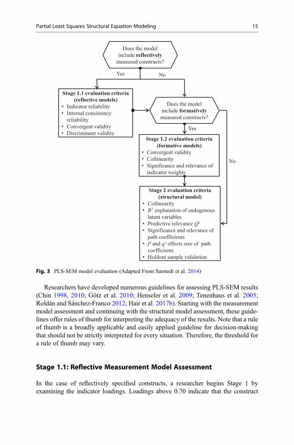
Researchers have developed numerous guidelines for assessing PLS-SEM results(Chin 1998, 2010; Götz et al. 2010; Henseler et al. 2009; Tenenhaus et al. 2005;Roldán and Sánchez-Franco 2012; Hair et al. 2017b). Starting with the measurementmodel assessment and continuing with the structural model assessment, these guide-lines offer rules of thumb for interpreting the adequacy of the results. Note that a ruleof thumb is a broadly applicable and easily applied guideline for decision-makingthat should not be strictly interpreted for every situation. Therefore, the threshold fora rule of thumb may vary.

Stage 1.1: Reflective Measurement Model Assessment

In the case of reflectively specified constructs, a researcher begins Stage 1 byexamining the indicator loadings. Loadings above 0.70 indicate that the construct

Yes

Stage 1.1 evaluation criteria(reflective models)

• Indicator reliability• Internal consistency

reliability• Convergent validity• Discriminant validity

No

Stage 1.2 evaluation criteria(formative models)

• Convergent validity• Collinearity• Significance and relevance of

indicator weights

Does the model include reflectively

measured constructs?

Does the model include formativelymeasured constructs?

Stage 2 evaluation criteria(structural model)

• Collinearity• R2 explanation of endogenous

latent variables • Predictive relevance Q2

• Significance and relevance of path coefficients

• f² and q² effects size of path coefficients

• Holdout sample validation

Yes

No

Fig. 3 PLS-SEM model evaluation (Adapted From Sarstedt et al. 2014)


explains more than 50% of the indicator’s variance, demonstrating that the indicatorexhibits a satisfactory degree of reliability.

The next step involves the assessment of the constructs’ internal consistencyreliability. When using PLS-SEM, internal consistency reliability is generally eval-uated using Jöreskog’s (1971) composite reliability ρc, which is defined as follows(for standardized data):

ρc ¼PK

k¼1 lk

� �2PK

k¼1 lk

� �2þPK

k¼1 var ekð Þ, (4)

where lk symbolizes the standardized outer loading of the indicator variable k ofa specific construct measured with K indicators, ek is the measurement error ofindicator variable k, and var(ek) denotes the variance of the measurement error,which is defined as 1� l2k .

For the composite reliability criterion, higher values indicate higher levels ofreliability. For instance, researchers can consider values between 0.60 and 0.70 as“acceptable in exploratory research,” whereas results between 0.70 and 0.95 repre-sent “satisfactory to good” reliability levels (Hair et al. 2017b, p. 112). However,values that are too high (e.g., higher than 0.95) are problematic, as they suggest thatthe items are almost identical and redundant. The reason may be (almost) the sameitem questions in a survey or undesirable response patterns such as straight lining(Diamantopoulos et al. 2012).

Cronbach’s alpha is another measure of internal consistency reliability that assumesthe same thresholds but yields lower values than the composite reliability (ρc). Thisstatistic is defined in its standardized form as follows, where K represents the con-struct’s number of indicators and �r the average nonredundant indicator correlationcoefficient (i.e., the mean of the lower or upper triangular correlation matrix):

Cronbach0s α ¼ K � r1þ K � 1ð Þ � r½ � : (5)

Generally, in PLS-SEM Cronbach’s alpha is the lower bound, while ρc is the upperbound of internal consistency reliability when estimating reflective measurementmodels with PLS-SEM. Researchers should therefore consider both measures intheir internal consistency reliability assessment. Alternatively, they may also considerassessing the reliability coefficient ρA (Dijkstra and Henseler 2015b), which usuallyreturns a value between Cronbach’s alpha and the composite reliability ρc.

The next step in assessing reflective measurement models addresses convergentvalidity, which is the extent to which a construct converges in its indicators byexplaining the items’ variance. Convergent validity is assessed by the averagevariance extracted (AVE) across all items associated with a particular construct andis also referred to as communality. The AVE is calculated as the mean of the squaredloadings of each indicator associated with a construct (for standardized data):


AVE ¼PK

k¼1 l2k

� �K

, (6)

where lk and K are defined as explained above. An acceptable threshold for the AVEis 0.50 or higher. This level or higher indicates that, on average, the constructexplains (more than) 50% of the variance of its items.

Once the reliability and the convergent validity of reflectively measured con-structs have been successfully established, the final step is to assess their discrimi-nant validity. This analysis reveals to which extent a construct is empirically distinctfrom other constructs both in terms of how much it correlates with other constructsand how distinctly the indicators represent only this single construct. Discriminantvalidity assessment in PLS-SEM involves analyzing Henseler et al.’s (2015) hetero-trait-monotrait ratio (HTMT) of correlations. The HTMT criterion is defined as themean value of the indicator correlations across constructs (i.e., the heterotrait-heteromethod correlations) relative to the (geometric) mean of the average correla-tions of indicators measuring the same construct. The HTMTof the constructs Yi andYj with, respectively, Ki and Kj indicators is defined as follows:

HTMTij

¼ 1

KiKj

XKi

g¼1

XKj

h¼1rig, jh

|fflfflfflfflfflfflfflfflfflfflfflfflfflfflfflfflfflfflfflfflffl{zfflfflfflfflfflfflfflfflfflfflfflfflfflfflfflfflfflfflfflfflffl}average

heterotrait�heteromethodcorrelation

� 2

Ki Ki � 1ð Þ ∙XKi�1

g¼1

XKi

h¼gþ1rig, ih∙

2

Kj Kj � 1� � ∙XKj�1

g¼1

XKj

h¼gþ1rjg, jh

!12

|fflfflfflfflfflfflfflfflfflfflfflfflfflfflfflfflfflfflfflfflfflfflfflfflfflfflfflfflfflfflfflfflfflfflfflfflfflfflfflfflfflfflfflfflfflfflfflfflfflfflfflfflfflfflfflfflfflfflfflfflfflfflfflfflfflfflfflfflfflffl{zfflfflfflfflfflfflfflfflfflfflfflfflfflfflfflfflfflfflfflfflfflfflfflfflfflfflfflfflfflfflfflfflfflfflfflfflfflfflfflfflfflfflfflfflfflfflfflfflfflfflfflfflfflfflfflfflfflfflfflfflfflfflfflfflfflfflfflfflfflffl}geometric mean of the average monotrait�heteromethod

correlation of construct Yi and the averagemonotrait�heteromethod correlation of construct Yj

,

(7)

where rig , jh represents the correlations of the indicators (i.e., within and across themeasurement models of latent variables Yi and Yj). Figure 4 shows the correlationmatrix of the six indicators used in the reflective measurement models of constructsY2 and Y3 from Fig. 1.

Therefore, high HTMT values indicate discriminant validity problems. Based onprior research and their simulation study results, Henseler et al. (2015) suggest athreshold value of 0.90 if the path model includes constructs that are conceptuallyvery similar (e.g., affective satisfaction, cognitive satisfaction, and loyalty); that is,in this situation, an HTMT value exceeding 0.90 suggests a lack of discriminantvalidity. However, when the constructs in the path model are conceptually moredistinct, researchers should consider 0.85 as threshold for HTMT (Henseler et al.2015). Furthermore, using the bootstrapping procedure, researchers can formally testwhether the HTMT value is significantly lower than one (also referred to asHTMTinference).


Stage 1.2: Formative Measurement Model Assessment

Formatively specified constructs are evaluated differently from reflectively mea-sured constructs. Their evaluation involves examination of (1) the convergentvalidity, (2) indicator collinearity, and (3) statistical significance and relevance ofthe indicator weights – see Fig. 3.

The convergent validity of formatively measured constructs is determined on thebasis of the extent to which the construct correlates with a reflectively measured (orsingle-item) construct capturing the same concept (also referred to as redundancyanalysis; Chin 1998). Accordingly, researchers must plan for the assessment ofconvergent validity in the research design stage by including a reflectively measuredconstruct, or single-item measure, of the formatively measured construct in the finalquestionnaire. Note that one should generally try to avoid using single items forconstruct measurement. Single items exhibit significantly lower levels of predictivevalidity compared to multi-item scales (Sarstedt et al. 2016a), which can be particu-larly problematic when using a variance-based analysis technique such as PLS-SEM.

Collinearity assessment involves computing each item’s variance inflation factor(VIF) by running a multiple regression of each indicator in the measurement modelof the formatively measured construct on all the other items of the same construct.The R2 values of the k-th regression facilitate the computation of the VIF for the k-thindicator, using the following formula:

VIFk ¼ 1

1� R2k

(8)

HigherR2 values in the k-th regression imply that the variance of the k-th item can beexplained by the other items in the same measurement model, which indicates collin-earity issues. Likewise, the higher theVIF, the greater the level of collinearity. As a ruleof thumb, VIF values above 5 are indicative of collinearity among the indicators.

Trait Y2 Y3

Trait Method x4 x5 x6 x7 x8 x9

Y2

x4 1

x5 r4,5 1

x6 r4,6 r5,6 1

Y3

x7 r4,7 r5,7 r6,7 1

x8 r4,8 r5,8 r6,8 r7,8 1

x9 r4,9 r5,9 r6,9 r7,9 r8,9 1

monotrait-heteromethod correlations

monotrait-heteromethod correlations

heterotrait-heteromethod correlations

Fig. 4 Correlation matrix example


The third step in assessing formatively measured constructs is examining thestatistical significance and relevance (i.e., the size) of the indicator weights. In contrastto regression analysis, PLS-SEM does not make any distributional assumptionsregarding the error terms that would facilitate the immediate testing of the weights’significance based on, for example, the normal distribution. Instead, the researchermust run bootstrapping, a procedure that draws a large number of subsamples (typi-cally 5,000) from the original data with replacement. The model is then estimated foreach of the subsamples, yielding a high number of estimates for eachmodel parameter.

Using the subsamples from bootstrapping, the researcher can construct a distribu-tion of the parameter under consideration and compute bootstrap standard errors,which allow for determining the statistical significance of the original indicatorweights. More precisely, bootstrap standard errors allow for computing t values (andcorresponding p values).When interpreting the results, reviewers and editors should beaware that bootstrapping is a random process, which yields different results every timeit is initiated. While the results from one bootstrapping run to the next generally do notdiffer fundamentally when using a large number of bootstrap samples such as 5,000,bootstrapping-based p values slightly lower than a predefined cutoff level should giverise to concern. In such a case, researchers may have repeatedly applied bootstrappinguntil a certain parameter has become significant, a practice referred to as p-hacking.

As an alternative, researchers can use the bootstrapping results to construct differenttypes of confidence intervals. Recent research by Aguirre-Urreta and Rönkkö (2017) inthe context of PLSc shows that bias-corrected and accelerated (BCa) bootstrap confi-dence intervals (Efron and Tibshirani 1993) perform very well in terms of coverage (i.e.,the proportion of times the population value of the parameter is included in the 1-α%confidence interval in repeated samples) and balance (i.e., how α% of cases fall to theright or to the left of the interval). If a weight’s confidence interval includes zero, thisprovides evidence that the weight is not statistically significant, making the indicator acandidate for removal from the measurement model. However, instead of mechanicallydeleting the indicator, researchers should first consider its loading, which represents theindicator’s absolute contribution to the construct. While an indicator might not have astrong relative contribution (e.g., because of the great number of indicators in theformative measurement model), its absolute contribution can still be substantial(Cenfetelli and Bassellier 2009). Based on these considerations, the following rules ofthumb apply (Hair et al. 2017b):

• If the weight is statistically significant, the indicator is retained.• If the weight is nonsignificant, but the indicator’s loading is 0.50 or higher, the

indicator is still retained if theory and expert judgment support its inclusion.• If the weight is nonsignificant and the loading is low (i.e., below 0.50), the

indicator should be deleted from the measurement model.

Researchers must be cautious when deleting formative indicators based onstatistical outcomes for at least the following two reasons. First, the indicator weightis a function of the number of indicators used to measure a construct: The higher thenumber of indicators, the lower their average weight. In other words, formative


measurement models have an inherent limit to the number of indicators that canretain a statistically significant weight (e.g., Cenfetelli and Bassellier 2009). Second,as formative indicators define the construct’s empirical meaning, indicator deletionshould be considered with caution and should generally be the exception. Contentvalidity considerations are imperative before deleting formative indicators (e.g.,Diamantopoulos and Winklhofer 2001).

Having assessed the formative indicator weights’ statistical significance, the finalstep is to examine each indicator’s relevance for shaping the construct (i.e., therelevance). In terms of relevance, indicator weights are standardized to values thatare usually between �1 and þ1, with weights closer to þ1 (or �1) representingstrong positive (or negative) relationships, and weights closer to 0 indicating weakrelationships. Note that values below �1 and above þ1 may technically occur, forinstance, when collinearity is at critical levels.

Stage 2: Structural Model Assessment

Provided the measurement model assessment indicates satisfactory quality, theresearcher moves to the assessment of the structural model in Stage 2 of the PLS-SEM evaluation process (Fig. 3). After checking for potential collinearity issuesamong the constructs, this stage primarily focuses on learning about the predictivecapabilities of the model, as indicated by the following criteria: coefficient ofdetermination (R2), cross-validated redundancy (Q2), and the path coefficients.

Computation of the path coefficients linking the constructs is based on a seriesof regression analyses. Therefore, the researcher must ascertain that collinearityissues do not bias the regression results. This step is analogous to the formativemeasurement model assessment, with the difference that the scores of the exogenouslatent variables serve as input for the VIF assessments. VIF values above 5 areindicative of collinearity among the predictor constructs.

The next step involves reviewing the R2, which indicates the variance explainedin each of the endogenous constructs. The R2 ranges from 0 to 1, with higher levelsindicting more predictive accuracy. As a rough rule of thumb, the R2 values of 0.75,0.50, and 0.25 can be considered substantial, moderate, and weak (Henseler et al.2009; Hair et al. 2011). It is important to note, however, that, in some researchcontexts, R2 values of 0.10 are considered satisfactory, for example, in the context ofpredicting stock returns (e.g., Raithel et al. 2012). Against this background, theresearcher should always interpret the R2 in the context of the study at hand byconsidering R2 values from related studies.

In addition to evaluating the R2 values of all endogenous constructs, the change inthe R2 value when a specific predictor construct is omitted from the model can beused to evaluate whether the omitted construct has a substantive impact on theendogenous constructs. This measure is referred to as the ƒ2 effect size and can becalculated as


f 2 ¼ R2included � R2

excluded

1� R2included

(9)

where R2included and R

2excluded are the R

2 values of the endogenous latent variable whena specific predictor construct is included in or excluded from the model. Technically,the change in the R2 values is calculated by estimating a specific partial regression inthe structural model twice (i.e., with the same latent variable scores). First, it isestimated with all exogenous latent variables included (yielding R2

included ) and,second, with a selected exogenous latent variable excluded (yielding R2

excluded). Asa guideline, ƒ2 values of 0.02, 0.15, and 0.35, respectively, represent small, medium,and large effects (Cohen 1988) of an exogenous latent variable. Effect size values ofless than 0.02 indicate that there is no effect.

Another means to assess the model’s predictive accuracy is the Q2 value (Geisser1974; Stone 1974). The Q2 value builds on the blindfolding procedure, which omitssingle points in the data matrix, imputes the omitted elements, and estimates themodel parameters. Using these estimates as input, the blindfolding procedure pre-dicts the omitted data points. This process is repeated until every data point has beenomitted and the model reestimated. The smaller the difference between the predictedand the original values, the greater the Q2 criterion and, thus, the model’s predictiveaccuracy and relevance. As a rule of thumb, Q2 values larger than zero for aparticular endogenous construct indicate that the path model’s predictive accuracyis acceptable for this particular construct.

To initiate the blindfolding procedure, researchers need to determine the sequence ofdata points to be omitted in each run. An omission distance of 7, for example, impliesthat every seventh data point of the endogenous construct’s indicators is eliminated in asingle blindfolding run. Hair et al. (2017a) suggest using an omission distance between5 and 10. Furthermore, there are two approaches to calculating the Q2 value: cross-validated redundancy and cross-validated communality, the former of which is gener-ally recommended to explore the predictive relevance of the PLS path model (Wold1982). Analogous to the f2 effect size, researchers can also analyze the q2 effect size,which indicates the change in the Q2 value when a specified exogenous construct isomitted from the model. As a relative measure of predictive relevance, q2 values of0.02, 0.15, and 0.35 indicate that an exogenous construct has a small, medium, or largepredictive relevance, respectively, for a certain endogenous construct.

A downside of these metrics is that they tend to overfit a particular sample ifpredictive validity is evaluated in the same sample used for estimation (Shmueli2010). This critique holds particularly for the R2, which is considered a measure ofthe model’s predictive accuracy in terms of in-sample prediction (Rigdon 2012).Predictive validity assessment, however, requires assessing prediction on thegrounds of holdout samples. But the overfitting problem also applies to the Q2

values, whose computation does not draw on holdout samples, but on single datapoints (as opposed to entire observations) being omitted and imputed. Hence, the Q2

values can only be partly considered a measure of out-of-sample prediction, becausethe sample structure remains largely intact in its computation. As Shmueli et al.


(2016) point out, “fundamental to a proper predictive procedure is the ability topredict measurable information on new cases.” As a remedy, Shmueli et al. (2016)developed the PLSpredict procedure for generating holdout sample-based pointpredictions in PLS path models on an item or construct level.

Subsequently, the strength and significance of the path coefficients is evaluatedregarding the relationships (structural paths) hypothesized between the constructs.Similar to the assessment of formative indicator weights, the significance assessmentbuilds on bootstrapping standard errors as a basis for calculating t and p values of pathcoefficients, or – as recommended in recent literature – their (bias-corrected andaccelerated) confidence intervals (Aguirre-Urreta and Rönkkö 2017). A path coeffi-cient is significant at the 5% probability of error level if zero does not fall into the 95%(bias-corrected and accelerated) confidence interval. For example, a path coefficientof 0.15 with 0.1 and 0.2 as lower and upper bounds of the 95% (bias-corrected andaccelerated) confidence interval would be considered significant since zero does notfall into this confidence interval. On the contrary, with a lower bound of�0.05 and anupper bound of 0.35, we would consider this coefficient as not significant.

In terms of relevance, path coefficients are usually between �1 to þ1, withcoefficients closer to þ1 representing strong positive relationships, and those closerto �1 indicating strong negative relationships (note that values below �1 and aboveþ1 may technically occur, for instance, when collinearity is at critical levels). A pathcoefficient of say 0.5 implies that if the independent construct increases by onestandard deviation unit, the dependent construct will increase by 0.5 standard deviationunits when keeping all other independent constructs constant. Determining whetherthe size of the coefficient is meaningful should be decided within the research context.When examining the structural model results, researchers should also interpret totaleffects. These correspond to the sum of the direct effect and all indirect effects betweentwo constructs in the path model.With regard to the path model shown in Fig. 1, Y1 hasa direct effect (b1) and an indirect effect (b2� b3) via Y2 on the endogenous construct Y3.Hence, the total effect of Y1 on Y3 is b1 + b2� b3. The examination of total effectsbetween constructs, including all their indirect effects, provides a more comprehensivepicture of the structural model relationships (Nitzl et al. 2016).

Research Application

Corporate Reputation Model

The empirical application builds on the corporate reputation model and data that Hairet al. (2017b) use in their book Primer on Partial Least Squares Structural EquationModeling (PLS-SEM), and that Hair et al. (2018) also employ in their AdvancedIssues in Partial Least Squares Structural Equation Modeling. The PLS path modelcreation and estimation draws on the software SmartPLS 3. The software, modelfiles, and datasets used in this market research application can be downloaded athttp://www.smartpls.com.


http://www.smartpls.com

Figure 5 shows the corporate reputation model as displayed in SmartPLS 3.Originally presented by Eberl (2010), the goal of this model is to explain the effectsof corporate reputation on customer satisfaction (CUSA) and, ultimately, customerloyalty (CUSL). Corporate reputation represents a company’s overall evaluation byits stakeholder (Helm et al. 2010), which comprises two dimensions (Schwaiger2004). The first dimension captures cognitive evaluations of the company, and theconstruct is the company’s competence (COMP). The second dimension capturesaffective judgments, which determine the company’s likeability (LIKE). This two-dimensional reputation measurement has been validated in different countries andapplied in various research studies (e.g., Eberl and Schwaiger 2005; Raithel andSchwaiger 2015; Schloderer et al. 2014). Research has shown that the approachperforms favorably (in terms of convergent validity and predictive validity) com-pared with alternative reputation measures (e.g., Sarstedt et al. 2013). Schwaiger(2004) also identified four exogenous constructs that represent the key sources of thetwo corporate reputation dimensions: (1) the quality of a company’s products andservices, as well as the quality of its customer orientation (QUAL); (2) the company’seconomic and managerial performance (PERF); (3) the company’s corporate socialresponsibility (CSOR); and (4) the company’s attractiveness (ATTR).

In terms of construct measurement, COMP, LIKE, and CUSL have reflectivelyspecified measurement models with three items. CUSA draws – for illustrativepurposes – on a single-item measure. The four exogenous latent variables QUAL,PERF, CSOR, and ATTR have formative measurement models. Table 2 provides anoverview of all items’ wordings.

qual_1

perf_1

perf_2

perf_3

perf_4

perf_5

csor_1

csor_2

csor_3

csor_4

csor_5

qual_2 qual_3 qual_4 qual_5 qual_6 qual_7 qual_8

comp_1 comp_2 comp_3

cusl_1

cusl_2

cusl_3

attr_3

like_3like_2like_1

cusa

attr_2attr_1

COMP

CUSLCUSA

CSOR

ATTR

LIKE

PERF

QUAL

Fig. 5 Corporate reputation model in SmartPLS 3


Table 2 Item wordings (Hair et al. 2017b)

Attractiveness (ATTR) – formative

attr_1 [The company] is successful in attracting high-quality employees

attr_2 I could see myself working at [the company]

attr_3 I like the physical appearance of [the company] (company, buildings, shops, etc.)

Competence (COMP) – reflective

comp_1 [The company] is a top competitor in its market

comp_2 As far as I know, [the company] is recognized worldwide

comp_3 I believe that [the company] performs at a premium level

Corporate Social Responsibility (CSOR) – formative

csor_1 [The company] behaves in a socially conscious way

csor_2 [The company] is forthright in giving information to the public

csor_3 [The company] has a fair attitude toward competitors

csor_4 [The company] is concerned about the preservation of the environment

csor_5 [The company] is not only concerned about profits

Customer loyalty (CUSL) – reflective

cusl_1 I would recommend [company] to friends and relatives.

cusl_2 If I had to choose again, I would choose [company] as my mobile phone servicesprovider

cusl_3 I will remain a customer of [company] in the future

Customer satisfaction (CUSA) – single item

cusa If you consider your experiences with [company], how satisfied are you with[company]?

Likeability (LIKE) – reflective

like_1 [The company] is a company that I can better identify with than other companies

like_2 [The company] is a company that I would regret more not having if it no longer existedthan I would other companies

like_3 I regard [the company] as a likeable company

Quality (QUAL) – formative

qual_1 The products/services offered by [the company] are of high quality

qual_2 [The company] is an innovator, rather than an imitator with respect to [industry]

qual_3 [The company]’s products/services offer good value for money

qual_4 The services [the company] offers are good

qual_5 Customer concerns are held in high regard at [the company]

qual_6 [The company] is a reliable partner for customers

qual_7 [The company] is a trustworthy company

qual_8 I have a lot of respect for [the company]

Performance (PERF) – formative

perf_1 [The company] is a very well-managed company

perf_2 [The company] is an economically stable company

perf_3 The business risk for [the company] is modest compared to its competitors

perf_4 [The company] has growth potential

perf_5 [The company] has a clear vision about the future of the company


Data

The model estimation draws on data from four German mobile communicationsnetwork providers. A total of 344 respondents rated the questions related to the itemson a 7-point Likert scale, whereby a value of 7 always represents the best possiblejudgment and a value of 1 the opposite. The most complex partial regression in thePLS path model has eight independent variables (i.e., the formative measurementmodel of QUAL). Hence, based on power statistics as suggested by, this sample sizeis technically large enough to estimate the PLS path model. Specifically, to detect R2

values of around 0.25 and assuming a power level of 80% and a significance level of5%, one would need merely 54 observations. The dataset has only 11 missing values,which are coded with the value �99. The maximum number of missing data pointsper item is 4 of 334 (1.16%) in cusl_2. Since the relative number of missing values isvery small, we continue the analysis by using the mean value replacement of missingdata option. Box plots diagnostic by means of IBM SPSS Statistics (see chapter 5 inSarstedt and Mooi 2014) reveals influential observations, but no outliers. Finally, theskewness and excess kurtosis values, as provided by the SmartPLS 3 data view,show that all the indicators are within the �1 and þ1 acceptable range. The onlyslight exception is the cusl_2 indicator (i.e., skewness of �1.30). However, thisdegree of non-normality of data in a single indicator is not a critical issue.

Model Estimation

The model estimation uses the basic PLS-SEM algorithm by Lohmöller (1989), thepath weighting scheme, a maximum of 300 iterations, a stop criterion of 0.0000001(or 1 � 10�7), and equal indicator weights for the initialization (default settings inthe SmartPLS 3 software). After running the algorithm, it is important to ascertainthat the algorithm converged (i.e., the stop criterion has been reached) and did notreach the maximum number of iterations. However, the PLS-SEM algorithm prac-tically always converges, even in very complex market research applications(Henseler 2010).

Figure 6 shows the PLS-SEM results. The numbers on the path relationshipsrepresent the standardized regression coefficients, while the numbers displayed inthe circles of the endogenous latent variables represent the R2 values. An initialassessment shows that CUSA has the strongest effect (0.505) on CUSL, followed byLIKE (0.344) and COMP (0.006). These three constructs explain 56.2% (i.e., the R2

value) of the variance of the endogenous construct CUSL. Similarly, we can interpretthe relationships between the exogenous latent variables ATTR, CSOR, PERF, andQUAL, as well as the two corporate reputation dimensions COMP and LIKE. Butbefore we address the interpretation of these results, we must assess the constructs’reflective and formative measurement models.


Results Evaluation

Reflective Measurement Model AssessmentThe evaluation of the PLS-SEM results begins with an assessment of the reflectivemeasurement models (i.e., COMP, CUSL, and LIKE). Table 3 shows the results andevaluation criteria outcomes. We find that all three reflective measurement modelsmeet the relevant assessment criteria. More specifically, all the outer loadings areabove 0.70, indicating that all indicators exhibit a sufficient level of reliability (i.e.,>0.50). Further, all AVE values are above 0.50, providing support for the measures’convergent validity. Composite reliability has values of 0.865 and higher, which isclearly above the expected minimum level of 0.70. Moreover, the Cronbach’s alphavalues range between 0.776 and 0.831, which is acceptable. Finally, all ρA valuesmeet the 0.70 threshold. These results suggest that the construct measures of COMP,CUSL, and LIKE exhibit sufficient levels of internal consistency reliability.

Finally, we assess the discriminant validity by using the HTMT criterion. All theresults are clearly below the conservative threshold of 0.85 (Table 4). Next, we runthe bootstrapping procedure with 5,000 samples and use the no sign changes option,BCa bootstrap confidence intervals, and two-tailed testing at the 0.05 significancelevel (which corresponds to a 95% confidence interval). The results show that noneof the HTMTconfidence intervals includes the value 1, suggesting that all the HTMTvalues are significantly different from 1. We thus conclude that discriminant validityhas been established.

qual_1

perf_1

perf_2

perf_3

perf_4

perf_5

csor_1

csor_2

csor_3

csor_4

csor_5

qual_2 qual_3

0.2020.041 0.106 0.160

0.3980.229

0.430

0.824 0.8440.821

0.631

0.146 0.006

0.5620.292

0.558

0.3440.436

0.8440.8690.880

0.295

0.059 0.380

0.0860.117

0.4680.1770.1940.340

0.199

0.0370.4060.0800.416

0.178

0.167

0.6580.4140.201

0.5050.833

0.843

0.9171.1000

−0.005

qual_4 qual_5 qual_6 qual_7 qual_8

comp_1 comp_2 comp_3

cusl_1

cusl_2

cusl_3

attr_3

like_3like_2like_1

cusa

attr_2attr_1

COMP

CUSLCUSA

CSOR

ATTR

LIKE

PERF

QUAL

0.190

0.306

Fig. 6 Corporate reputation model and PLS-SEM results


Table

3PLS-SEM

assessmentresults

ofreflectiv

emeasurementmod

els

Latentvariable

Indicators

Con

vergentvalid

ityInternalconsistencyreliability

Loading

sIndicatorreliability

AVE

Com

positereliabilityρ c

Reliabilityρ A

Cronb

ach’salph

a

>0.70

>0.50

>0.50

>0.70

>0.70

0.70

–0.90

COMP

comp_

10.82

40.67

90.68

80.86

90.78

60.77

6

comp_

20.82

10.67

4

comp_

30.84

40.71

2

CUSL

cusl_1

0.83

30.69

40.74

80.89

90.83

90.83

1

cusl_2

0.91

70.84

1

cusl_3

0.84

30.711

LIK

Elik

e_1

0.88

00.77

40.74

70.89

90.83

60.83

1

like_2

0.86

90.75

5

like_3

0.84

40.71

2


The CUSA construct is not included in the reflective (and subsequent formative)measurement model assessment, because it is a single-item construct. For thisconstruct indicator data and latent variable scores are identical. Consequently,CUSA does not have a measurement model, which can be assessed using thestandard evaluation criteria.

Formative Measurement Model AssessmentThe formative measurement model assessment initially focuses on the constructs’convergent validity by conducting a redundancy analysis of each construct (i.e.,ATTR, CSOR, PERF, and QUAL). The redundancy analysis draws on global singleitems, which summarize the essence each formatively measured construct purportsto measure. These single items have been included in the original questionnaire. Forexample, respondents had to answer the statement, “Please assess to which degree[the company] acts in socially conscious ways,” measured on a scale of 0 (not at all)to 10 (extremely). This question can be used as an endogenous single-item constructto validate the formative measurement of corporate social responsibility (CSOR). Forthis purpose, we need to create a new PLS path model for each formatively measuredconstruct that predicts the global measure as an endogenous single-item constructas shown in Fig. 7. All the path relationships between the formatively measuredconstruct and its global single-item measure (i.e., 0.874, 0.857, 0.811, and 0.805) areabove the critical value of 0.70. We thus conclude that convergent validity of theformatively measured constructs has been established.

Next, we assesswhether critical levels of collinearity substantially affect the formativeindicatorweight estimates.Wefind that the highestVIF value (i.e., 2.269 of the formativeindicator qual_3) is clearly below the threshold value of 5, suggesting that collinearity isnot at a critical level. Testing the indicator weights’ significance draws on thebootstrapping procedure (5,000 samples, no sign changes option, bootstrap confidenceintervals (BCa), two-tailed testing at the 0.05 significance level.) and produces the 95%BCa confidence intervals as shown in Table 5. The results show thatmost of the indicatorweights are significant, with the exception of csor_2, csor_4, qual_2, qual_3, andqual_4, whose indicator weight confidence intervals include the value 0. However,these indicators exhibit statistically significant loadings above the 0.50 threshold, pro-viding support for their absolute contribution to the constructs. In addition, prior researchhas substantiated the relevance of these indicators for the measurement of theCSOR andQUAL constructs (Eberl 2010; Schwaiger 2004; Sarstedt et al. 2013). Therefore, weretain the nonsignificant, but relevant, indicators in the formative measurement models.

Table 4 HTMT values

COMP CUSA CUSL LIKE

COMP

CUSA 0.465 [0.364;0.565]

CUSL 0.532 [0.421;0.638] 0.755 [0.684;0.814]

LIKE 0.780 [0.690;0.853] 0.577 [0.489;0.661] 0.737 [0.653;0.816]

Note: The values in the brackets represent the lower and the upper bounds of the 95% confidenceinterval


Fig.7

Redun

dancyanalysis


Table 5 Formative indicator weights and significance testing results

Formativeconstructs

Formativeindicators

Outer weights (Outerloadings)

95% BCaconfidenceinterval

Significant( p <0.05)?

ATTR attr_1 0.414 (0.755) [0.273,0.554]

Yes

attr_2 0.201 (0.506) [0.073,0.332]

Yes

attr_3 0.658 (0.891) [0.516,0.761]

Yes

CSOR csor_1 0.306 (0.771) [0.145,0.458]

Yes

csor_2 0.037 (0.571) [�0.082,0.167]

No

csor_3 0.406 (0.838) [0.229,0.550]

Yes

csor_4 0.080 (0.617) [�0.063,0.219]

No

csor_5 0.416 (0.848) [0.260,0.611]

Yes

PERF perf_1 0.468 (0.846) [0.310,0.582]

Yes

perf_2 0.177 (0.690) [0.044,0.311]

Yes

perf_3 0.194 (0.573) [0.069,0.298]

Yes

perf_4 0.340 (0.717) [0.205,0.479]

Yes

perf_5 0.199 (0.638) [0.070,0.350]

Yes

QUAL qual_1 0.202 (0.741) [0.103,0.332]

Yes

qual_2 0.041 (0.570) [�0.074,0.148]

No

qual_3 0.106 (0.749) [�0.004,0.227]

No

qual_4 �0.005 (0.664) [�0.119,0.081]

No

qual_5 0.160 (0.787) [0.045,0.267]

Yes

qual_6 0.398 (0.856) [0.275,0.501]

Yes

qual_7 0.229 (0.722) [0.094,0.328]

Yes

qual_8 0.190 (0.627) [0.060,0.303]

Yes


The results of the reflective and formative measurement model assessmentsuggest that all construct measures exhibit satisfactory levels of reliability andvalidity. We can therefore proceed with the assessment of the structural model.

Structural Model AssessmentFollowing the structural model assessment procedure (Fig. 3), we first need tocheck the structural model for collinearity issues by examining the VIF values ofall sets predictor constructs in the structural model. As all VIF values are belowthe threshold of 5, we can conclude that collinearity is not a critical issue. Whenanalyzing the path coefficient estimates of the structural model (Table 6), we startwith the key target construct CUSL on the right-hand side of the PLS path model(Fig. 6). The construct CUSA (0.505) has the strongest effect on CUSL, followed byLIKE (0.344), while the effect of COMP (0.006) is very close to zero. Bootstrappingresults substantiate that the effects of CUSA and LIKE on CUSL are significant,while COMP does not have a significant effect at the 5% probability of error level.Moreover, COMP has a significant but relatively small effect on CUSA (0.146),

Table 6 Path coefficients of the structural model and significance testing results

Pathcoefficient

95% BCa confidenceinterval

Significant( p <0.05)?

f2 effectsize

q2 effectsize

ATTR !COMP

0.086 [�0.013, 0.187] No 0.009 <0.001

ATTR !LIKE

0.167 [0.032, 0.273] Yes 0.030 0.016

COMP !CUSA

0.146 [0.033, 0.275] Yes 0.018 0.006

COMP !CUSL

0.006 [�0.111, 0.113] No <0.001 �0.002

CSOR !COMP

0.059 [�0.036, 0.156] No 0.005 �0.005

CSOR !LIKE

0.178 [0.084, 0.288] Yes 0.035 0.018

CUSA !CUSL

0.505 [0.428, 0.580] Yes 0.412 0.229

LIKE !CUSA

0.436 [0.312, 0.544] Yes 0.159 0.151

LIKE !CUSL

0.344 [0.241, 0.453] Yes 0.138 0.077

PERF !COMP

0.295 [0.172, 0.417] Yes 0.082 0.039

PERF !LIKE

0.117 [�0.012, 0.254] No 0.011 0.003

QUAL !COMP

0.430 [0.295, 0.560] Yes 0.143 0.052

QUAL !LIKE

0.380 [0.278, 0.514] Yes 0.094 0.050


while the effect of LIKE is relatively strong (0.436). We also find that the modelexplains 56.2% of CUSL’s variance (i.e., R2 = 0.562), which is relatively highconsidering that the model only considers the effects of customer satisfaction andthe rather abstract concept of corporate reputation as predictors of customer loyalty.With a value of 0.292, R2 of CUSA is clearly lower but still satisfactory, consideringthat only LIKE and COMP predict customer satisfaction in this model.

When analyzing the key predictors of LIKE, which has a substantial R2 value of0.558, we find that QUAL has the strongest significant effect (0.380), followed byCSOR (0.178), and ATTR (0.167); PERF (0.117) has the weakest effect on LIKE,which is not significant at the 5% level (Table 6). Corporate reputation’s cognitivedimension COMP also has a substantial R2 value of 0.631. Analyzing this construct’spredictors shows thatQUAL (0.430) and PERF (0.295) have the strongest significanteffects. On the contrary, the effects of ATTR (0.086) and CSOR (0.059) on COMP arenot significant at the 5% level. Analyzing the exogenous constructs’ total effects onCUSL shows that QUAL has the strongest total effect (0.248), followed by CSOR(0.105), ATTR (0.101), and PERF (0.089). These results suggest that companiesshould focus on marketing activities that positively influence the customers’ percep-tion of the quality of their products and services.

Table 6 also shows the f2 effect sizes. Relatively high f2 effect sizes occur for therelationships CUSA ➔ CUSL (0.412), LIKE ➔ CUSA (0.159), QUAL ➔ COMP(0.143), and LIKE➔ CUSL (0.138). These relationships also have particularly strongpath coefficients of 0.30 and higher. Interestingly, the relationship betweenQUAL andLIKE has a strong path coefficient of 0.380 but only a weak f2 effect size of 0.094. Allthe other f2 effect sizes in the structural model are weak and, if below 0.02, negligible.

Finally, we determine the predictive relevance of the PLS path model by carryingout the blindfolding procedure using an omission distance D = 7. The resultingcross-validated redundancy Q2 values are above zero for all endogenous constructs,providing support for the model’s predictive accuracy. More precisely, CUSL andCOMP have the highest Q2 values (0.415), followed by LIKE (0.406) and, finally,CUSA (0.280). Further analysis of the q2 shows that the relationships CUSA ➔CUSL (0.229) and LIKE➔ CUSA (0.151) have moderate q2 effect sizes of 0.15 andhigher. All other q2 effect sizes are weak and, if below 0.02, negligible.

Conclusions

Most prior research discussing the benefits and limitations of PLS-SEM or analyzingits performance (e.g., in terms of parameter estimation) has not acknowledged that themethod takes on a fundamentally different philosophy of measurement compared tofactor-based SEM (e.g., Rigdon et al. 2017). Rather than assuming a common factormodel structure, PLS-SEM draws on composite model logic to represent reflectiveand formative measurement models. The method linearly combines sets (or blocks) ofindicators to form composites that represent the conceptual variables and assesses theextent to which these measures are valid and reliable (Tenenhaus et al. 2005). In otherwords, PLS-SEM is an approximation method that inherently recognizes that


constructs and conceptual variables are not identical (Rigdon et al. 2017). For severalreasons, factor indeterminacy being the most prominent one, this view of measure-ment is more reasonable than the common factor model logic assumed by factor-based SEM, which equates constructs and conceptual variables. As Rigdon (2016, p.19) notes, “common factor proxies cannot be assumed to carry greater significancethan composite proxies in regard to the existence or nature of conceptual variables.”

PLS-SEM offers a good approximation of common factor models in situations wherefactor-based SEM cannot deliver results due to its methodological limitations in terms ofmodel complexity, sample size requirements, or inclusion of composite variables in themodel (Reinartz et al. 2009; Sarstedt et al. 2016b; Willaby et al. 2015). Dijkstra andHenseler’s (2015b) PLSc allows researchers mimicking factor-based SEM results whilebenefiting from the original PLS-SEM method’s flexibility in terms of model specifica-tion.However, such an analysis rests on the implicit assumption that factor-based SEM isthe correct estimator that delivers the true results as a benchmark for SEM.

While standard PLS-SEM analyses provide important insights into the strength andsignificance of the hypothesized model relationships, more advanced modeling andestimating techniques shed further light on the nature of the proposed relationships.Research has brought forward a variety of complementary analysis techniques andprocedures, which extend the methodological toolbox of researchers working with themethod. Examples of these methods include the confirmatory tetrad analysis (CTA-PLS), which enables researchers to statistically test if the measurement model operatio-nalization should rather build on effect or composite indicators (Gudergan et al. 2008),and latent class techniques, which allow assessing if unobserved heterogeneity affectsthe model estimates. Prominent examples of PLS-SEM-based latent class techniquesinclude finite mixture partial least squares (Hahn et al. 2002; Sarstedt et al. 2011a), PLSgenetic algorithm segmentation (Ringle et al. 2013, 2014), prediction-oriented segmen-tation (Becker et al. 2013b), and iterative reweighted regressions (Schlittgen et al. 2016).Further methods to account for heterogeneity in the structural model include the analysisof moderating effects (Henseler and Chin 2010), nonlinear effects (Henseler et al.2012a), and the multigroup analysis (Sarstedt et al. 2011b), including testing formeasurement invariance (Henseler et al. 2016b). A further complementary method, theimportance-performance map analysis (IPMA), facilitates richer outcome discussions inthat it extends the analysis of total effects in the model by adding a second resultsdimension to the analysis which incorporates the average values of the latent variables(Ringle and Sarstedt 2016). Hair et al. (2018) provide a more detailed overview andintroduction to these complementary techniques for more advanced PLS-SEM analyses.

Cross-References

▶Design and Process of Survey Research▶ Factor Analysis▶Regression Analysis▶ Structural Equation Modeling


http://link.springer.com/Design and Process of Survey Research

http://link.springer.com/Factor Analysis

http://link.springer.com/Regression Analysis

http://link.springer.com/Structural Equation Modeling

Acknowledgment This chapter uses the statistical software SmartPLS 3 (http://www.smartpls.com). Ringle acknowledges a financial interest in SmartPLS.

References

Aaker, D. A. (1991). Managing brand equity: Capitalizing on the value of a brand name. NewYork: Free Press.

Aguirre-Urreta, M. I., & Rönkkö, M. (2017). Statistical inference with PLSc using bootstrapconfidence intervals. MIS Quarterly, forthcoming.

Akter, S., Wamba, S. F., & Dewan, S. (2017). Why PLS-SEM is suitable for complex modeling? Anempirical illustration in big data analytics quality. Production Planning & Control, 28(11-12),1011–1021.

Ali, F., Rasoolemanesh, S. M., Sarstedt, M., Ringle, C. M., & Ryu, K. (2017). An assessment of theuse of partial least squares structural equation modeling (PLS-SEM) in hospitality research.International Journal of Contemporary Hospitality Management, forthcoming.

Baumgartner, H., & Homburg, C. (1996). Applications of structural equation modeling in market-ing and consumer research: A review. International Journal of Research in Marketing, 13(2),139–161.

Becker, J.-M., & Ismail, I. R. (2016). Accounting for sampling weights in PLS path modeling:Simulations and empirical examples. European Management Journal, 34(6), 606–617.

Becker, J.-M., Rai, A., & Rigdon, E. E. (2013a). Predictive validity and formative measurement instructural equation modeling: Embracing practical relevance. In: 2013 Proceedings of theinternational conference on information systems, Milan.

Becker, J.-M., Rai, A., Ringle, C. M., & Völckner, F. (2013b). Discovering unobserved heteroge-neity in structural equation models to avert validity threats. MIS Quarterly, 37(3), 665–694.

Bollen, K. A. (1989). Structural equations with latent variables. New York: Wiley.Bollen, K. A. (2002). Latent variables in psychology and the social sciences. Annual Review of

Psychology, 53(1), 605–634.Bollen, K. A. (2011). Evaluating effect, composite, and causal indicators in structural equation

models. MIS Quarterly, 35(2), 359–372.Bollen, K. A., & Bauldry, S. (2011). Three Cs in measurement models: Causal indicators, composite

indicators, and covariates. Psychological Methods, 16(3), 265–284.Bollen, K. A., & Diamantopoulos, A. (2017). In defense of causal–formative indicators: A minority

report. Psychological Methods, forthcoming.Bollen, K. A., & Lennox, R. (1991). Conventional wisdom on measurement: A structural equation

perspective. Psychological Bulletin, 110(2), 305–314.Borsboom, D., Mellenbergh, G. J., & van Heerden, J. (2003). The theoretical status of latent

variables. Psychological Review, 110(2), 203–219.Cenfetelli, R. T., & Bassellier, G. (2009). Interpretation of formative measurement in information

systems research. MIS Quarterly, 33(4), 689–708.Chin, W. W. (1998). The partial least squares approach to structural equation modeling. In G.

A. Marcoulides (Ed.), Modern methods for business research (pp. 295–358). Mahwah:Erlbaum.

Chin, W. W. (2010). How to write up and report PLS analyses. In: V. Esposito Vinzi, W. W. Chin, J.Henseler, & H. Wang (Eds.), Handbook of partial least squares: Concepts, methods andapplications (Springer Handbooks of Computational Statistics Series, Vol. II, pp. 655–690).Heidelberg/Dordrecht/London/New York: Springer.

Chin, W. W., Marcolin, B. L., & Newsted, P. R. (2003). A partial least squares latent variablemodeling approach for measuring interaction effects: Results from a Monte Carlo simulationstudy and an electronic-mail emotion/adoption study. Information Systems Research, 14(2),189–217.




Chou, C.-P., Bentler, P. M., & Satorra, A. (1991). Scaled test statistics and robust standard errors fornon-normal data in covariance structure analysis: A Monte Carlo study. British Journal ofMathematical and Statistical Psychology, 44(2), 347–357.

Cohen, J. (1988). Statistical power analysis for the behavioral sciences (2nd ed.). Mahwah:Lawrence Erlbaum Associates.

Coltman, T., Devinney, T. M., Midgley, D. F., & Venaik, S. (2008). Formative versus reflectivemeasurement models: Two applications of formative measurement. Journal of BusinessResearch, 61(12), 1250–1262.

Diamantopoulos, A. (2006). The error term in formative measurement models: Interpretation andmodeling implications. Journal of Modeling in Management, 1(1), 7–17.

Diamantopoulos, A. (2011). Incorporating formative measures into covariance-based structuralequation models. MIS Quarterly, 35(2), 335–358.

Diamantopoulos, A., &Winklhofer, H. M. (2001). Index construction with formative indicators: Analternative to scale development. Journal of Marketing Research, 38(2), 269–277.

Diamantopoulos, A., Sarstedt, M., Fuchs, C., Wilczynski, P., & Kaiser, S. (2012). Guidelines forchoosing between multi-item and single-item scales for construct measurement: A predictivevalidity perspective. Journal of the Academy of Marketing Science, 40(3), 434–449.

Dijkstra, T. K. (2010). Latent variables and indices: Herman world’s basic design and partial leastsquares. In V. Esposito Vinzi, W. W. Chin, J. Henseler, H. Wang (Eds.), Handbook of partialleast squares: Concepts, methods and applications (Springer Handbooks of ComputationalStatistics Series, Vol. II, pp. 23–46). Heidelberg/Dordrecht/London/New York: Springer.

Dijkstra, T. K., & Henseler, J. (2011). Linear indices in nonlinear structural equation models: Bestfitting proper indices and other composites. Quality & Quantity, 45(6), 1505–1518.

Dijkstra, T. K., & Henseler, J. (2015a). Consistent and asymptotically normal PLS estimators forlinear structural equations. Computational Statistics & Data Analysis, 81(1), 10–23.

Dijkstra, T. K., & Henseler, J. (2015b). Consistent partial least squares path modeling. MISQuarterly, 39(2), 297–316.

Dijkstra, T. K., & Schermelleh-Engel, K. (2014). Consistent partial least squares for nonlinearstructural equation models. Psychometrika, 79(4), 585–604.

do Valle, P. O., & Assaker, G. (2016). Using partial least squares structural equation modeling intourism research: A review of past research and recommendations for future applications.Journal of Travel Research, 55(6), 695–708.

Eberl, M. (2010). An application of PLS in multi-group analysis: The need for differentiatedcorporate-level marketing in the mobile communications industry. In: V. Esposito Vinzi, W.W. Chin, J. Henseler, & H. Wang (Eds.), Handbook of partial least squares: Concepts, methodsand applications (Springer Handbooks of Computational Statistics Series, Vol. II, pp. 487–514).Heidelberg/Dordrecht/London/New York: Springer.

Eberl, M., & Schwaiger, M. (2005). Corporate reputation: Disentangling the effects on financialperformance. European Journal of Marketing, 39(7/8), 838–854.

Edwards, J. R., & Bagozzi, R. P. (2000). On the nature and direction of relationships betweenconstructs and measures. Psychological Methods, 5(2), 155–174.

Efron, B., & Tibshirani, R. J. (1993). An introduction to the bootstrap. New York: Chapman & Hall.Esposito Vinzi, V., Chin, W. W., Henseler, J., & Wang, H. (Eds.) (2010). Handbook of partial least

squares: Concepts, methods and applications (Springer Handbooks of Computational StatisticsSeries, Vol. II). Heidelberg/Dordrecht/London/New York: Springer.

Evermann, J., & Tate, M. (2016). Assessing the predictive performance of structural equation modelestimators. Journal of Business Research, 69(10), 4565–4582.

Falk, R. F., & Miller, N. B. (1992). A primer for soft modeling. Akron: University of Akron Press.Fornell, C. G., & Bookstein, F. L. (1982). Two structural equation models: LISREL and PLS

applied to consumer exit-voice theory. Journal of Marketing Research, 19(4), 440–452.Garson, G. D. (2016). Partial least squares regression and structural equation models. Asheboro:

Statistical Associates.Geisser, S. (1974). A predictive approach to the random effects model. Biometrika, 61(1), 101–107.


Goodhue, D. L., Lewis, W., & Thompson, R. (2012). Does PLS have advantages for small samplesize or non-normal data? MIS Quarterly, 36(3), 981–1001.

Götz, O., Liehr-Gobbers, K., & Krafft, M. (2010). Evaluation of structural equation models usingthe partial least squares (PLS) approach. In: V. Esposito Vinzi, W. W. Chin, J. Henseler, & H.Wang (Eds.), Handbook of partial least squares: Concepts, methods and applications (SpringerHandbooks of Computational Statistics Series, Vol. II, pp. 691–711). Heidelberg/Dordrecht/London/New York: Springer.

Grace, J. B., & Bollen, K. A. (2008). Representing general theoretical concepts in structuralequation models: The role of composite variables. Environmental and Ecological Statistics,15(2), 191–213.

Gregor, S. (2006). The nature of theory in information systems. MIS Quarterly, 30(3), 611–642.Gudergan, S. P., Ringle, C. M., Wende, S., & Will, A. (2008). Confirmatory tetrad analysis in PLS

path modeling. Journal of Business Research, 61(12), 1238–1249.Haenlein, M., & Kaplan, A. M. (2004). A beginner’s guide to partial least squares analysis.

Understanding Statistics, 3(4), 283–297.Hahn, C., Johnson, M. D., Herrmann, A., & Huber, F. (2002). Capturing customer heterogeneity

using a finite mixture PLS approach. Schmalenbach Business Review, 54(3), 243–269.Hair, J. F., Ringle, C. M., & Sarstedt, M. (2011). PLS-SEM: Indeed a silver bullet. Journal of

Marketing Theory and Practice, 19(2), 139–151.Hair, J. F., Sarstedt, M., Pieper, T. M., & Ringle, C. M. (2012a). The use of partial least squares

structural equation modeling in strategic management research: A review of past practices andrecommendations for future applications. Long Range Planning, 45(5–6), 320–340.

Hair, J. F., Sarstedt, M., Ringle, C. M., & Mena, J. A. (2012b). An assessment of the use of partialleast squares structural equation modeling in marketing research. Journal of the Academy ofMarketing Science, 40(3), 414–433.

Hair, J. F., Ringle, C. M., & Sarstedt, M. (2013). Partial least squares structural equation modeling:Rigorous applications, better results and higher acceptance. Long Range Planning, 46(1–2),1–12.

Hair, J. F., Hollingsworth, C. L., Randolph, A. B., & Chong, A. Y. L. (2017a). An updated andexpanded assessment of PLS-SEM in information systems research. Industrial Management &Data Systems, 117(3), 442–458.

Hair, J. F., Hult, G. T. M., Ringle, C. M., & Sarstedt, M. (2017b). A primer on partial least squaresstructural equation modeling (PLS-SEM) (2nd ed.). Thousand Oaks: Sage.

Hair, J. F., Hult, G. T. M., Ringle, C. M., Sarstedt, M., & Thiele, K. O. (2017c). Mirror, mirror on thewall: A comparative evaluation of composite-based structural equation modeling methods.Journal of the Academy of Marketing Science, forthcoming.

Hair, J. F., Sarstedt, M., Ringle, C. M., & Gudergan, S. P. (2018). Advanced issues in partial leastsquares structural equation modeling (PLS-SEM). Thousand Oaks: Sage.

Helm, S., Eggert, A., & Garnefeld, I. (2010). Modelling the impact of corporate reputation oncustomer satisfaction and loyalty using PLS. In V. Esposito Vinzi, W. W. Chin, J. Henseler, & H.Wang (Eds.), Handbook of partial least squares: Concepts, methods and applications (SpringerHandbooks of Computational Statistics Series, Vol. II, pp. 515–534). Heidelberg/Dordrecht/London/New York: Springer.

Henseler, J. (2010). On the convergence of the partial least squares path modeling algorithm.Computational Statistics, 25(1), 107–120.

Henseler, J. (2017). Using variance-based structural equation modeling for empirical advertisingresearch at the interface of design and behavioral research. Journal of Advertising, 46(1),178–192.

Henseler, J., & Chin, W. W. (2010). A comparison of approaches for the analysis of interactioneffects between latent variables using partial least squares path modeling. Structural EquationModeling, 17(1), 82–109.

Henseler, J., & Sarstedt, M. (2013). Goodness-of-fit indices for partial least squares path modeling.Computational Statistics, 28(2), 565–580.


Henseler, J., Ringle, C. M., & Sinkovics, R. R. (2009). The use of partial least squares pathmodeling in international marketing. In R. R. Sinkovics & P. N. Ghauri (Eds.), Advances ininternational marketing (Vol. 20, pp. 277–320). Bingley: Emerald.

Henseler, J., Fassott, G., Dijkstra, T. K., & Wilson, B. (2012a). Analyzing quadratic effects offormative constructs by means of variance-based structural equation modelling. EuropeanJournal of Information Systems, 21(1), 99–112.

Henseler, J., Ringle, C. M., & Sarstedt, M. (2012b). Using partial least squares path modeling ininternational advertising research: Basic concepts and recent issues. In S. Okazaki (Ed.),Handbook of research in international advertising (pp. 252–276). Cheltenham: Edward ElgarPublishing.

Henseler, J., Dijkstra, T. K., Sarstedt, M., Ringle, C. M., Diamantopoulos, A., Straub, D. W.,Ketchen, D. J., Hair, J. F., Hult, G. T. M., & Calantone, R. J. (2014). Common beliefs and realityabout partial least squares: Comments on Rönkkö & Evermann (2013). OrganizationalResearch Methods, 17(2), 182–209.

Henseler, J., Ringle, C. M., & Sarstedt, M. (2015). A new criterion for assessing discriminantvalidity in variance-based structural equation modeling. Journal of the Academy of MarketingScience, 43(1), 115–135.

Henseler, J., Hubona, G. S., & Ray, P. A. (2016a). Using PLS path modeling in new technologyresearch: Updated guidelines. Industrial Management & Data Systems, 116(1), 1–19.

Henseler, J., Ringle, C. M., & Sarstedt, M. (2016b). Testing measurement invariance of compositesusing partial least squares. International Marketing Review, 33(3), 405–431.

Houston, M. B. (2004). Assessing the validity of secondary data proxies for marketing constructs.Journal of Business Research, 57(2), 154–161.

Hu, L.-t., & Bentler, P. M. (1998). Fit indices in covariance structure modeling: Sensitivity tounderparameterized model misspecification. Psychological Methods, 3(4), 424–453.

Hui, B. S., & Wold, H. O. A. (1982). Consistency and consistency at large of partial least squaresestimates. In K. G. Jöreskog & H. O. A. Wold (Eds.), Systems under indirect observation, part II(pp. 119–130). Amsterdam: North Holland.

Jöreskog, K. G. (1971). Simultaneous factor analysis in several populations. Psychometrika, 36(4),409–426.

Jöreskog, K. G. (1973). A general method for estimating a linear structural equation system. In A.S. Goldberger & O. D. Duncan (Eds.), Structural equation models in the social sciences (pp.255–284). New York: Seminar Press.

Jöreskog, K. G., & Wold, H. O. A. (1982). The ML and PLS techniques for modeling with latentvariables: Historical and comparative aspects. In H. O. A. Wold & K. G. Jöreskog (Eds.),Systems under indirect observation, part I (pp. 263–270). Amsterdam: North-Holland.

Kaufmann, L., & Gaeckler, J. (2015). A structured review of partial least squares in supply chainmanagement research. Journal of Purchasing and Supply Management, 21(4), 259–272.

Kock, N., & Hadaya, P. (2017). Minimum sample size estimation in PLS-SEM: The inverse squareroot and gamma-exponential methods. Information Systems Journal, forthcoming.

Latan, H., & Noonan, R. (Eds.). (2017). Partial least squares structural equation modeling: Basicconcepts, methodological issues and applications. Heidelberg: Springer.

Lee, L., Petter, S., Fayard, D., & Robinson, S. (2011). On the use of partial least squares pathmodeling in accounting research. International Journal of Accounting Information Systems,12(4), 305–328.

Lei, P.-W., & Wu, Q. (2012). Estimation in structural equation modeling. In R. H. Hoyle (Ed.),Handbook of structural equation modeling (pp. 164–179). New York: Guilford Press.

Lohmöller, J.-B. (1989). Latent variable path modeling with partial least squares. Heidelberg:Physica.

Marcoulides, G. A., & Chin, W. W. (2013). You write, but others read: Common methodologicalmisunderstandings in PLS and related methods. In H. Abdi, W. W. Chin, V. Esposito Vinzi, G.Russolillo, & L. Trinchera (Eds.), New perspectives in partial least squares and related methods(Springer Proceedings in Mathematics & Statistics, Vol. 56, pp. 31–64). New York: Springer.


Marcoulides, G. A., & Saunders, C. (2006). PLS: A silver bullet? MIS Quarterly, 30(2), III–IIX.Marcoulides, G. A., Chin, W. W., & Saunders, C. (2009). Foreword: A critical look at partial least

squares modeling. MIS Quarterly, 33(1), 171–175.Marcoulides, G. A., Chin, W. W., & Saunders, C. (2012). When imprecise statistical statements

become problematic: A response to Goodhue, Lewis, and Thompson. MIS Quarterly, 36(3),717–728.

Mateos-Aparicio, G. (2011). Partial least squares (PLS) methods: Origins, evolution, and applica-tion to social sciences. Communications in Statistics – Theory and Methods, 40(13),2305–2317.

McDonald, R. P. (1996). Path analysis with composite variables.Multivariate Behavioral Research,31(2), 239–270.

Nitzl, C. (2016). The use of partial least squares structural equation modelling (PLS-SEM) inmanagement accounting research: Directions for future theory development. Journal ofAccounting Literature, 37, 19–35.

Nitzl, C., & Chin, W. W. (2017). The case of partial least squares (PLS) path modeling inmanagerial accounting. Journal of Management Control, 28(2), 137–156.

Nitzl, C., Roldán, J. L., & Cepeda Carrión, G. (2016). Mediation analysis in partial least squarespath modeling: Helping researchers discuss more sophisticated models. Industrial Management& Data Systems, 119(9), 1849–1864.

Noonan, R., & Wold, H. O. A. (1982). PLS path modeling with indirectly observed variables: Acomparison of alternative estimates for the latent variable. In K. G. Jöreskog & H. O. A. Wold(Eds.), Systems under indirect observations: Part II (pp. 75–94). Amsterdam: North-Holland.

Nunnally, J. C., & Bernstein, I. (1994). Psychometric theory (3rd ed.). New York: McGraw Hill.Olsson, U. H., Foss, T., Troye, S. V., & Howell, R. D. (2000). The performance of ML, GLS, and

WLS estimation in structural equation modeling under conditions of misspecification andnonnormality. Structural Equation Modeling: A Multidisciplinary Journal, 7(4), 557–595.

Peng, D. X., & Lai, F. (2012). Using partial least squares in operations management research: Apractical guideline and summary of past research. Journal of Operations Management, 30(6),467–480.

Raithel, S., & Schwaiger, M. (2015). The effects of corporate reputation perceptions of the generalpublic on shareholder value. Strategic Management Journal, 36(6), 945–956.

Raithel, S., Sarstedt, M., Scharf, S., & Schwaiger, M. (2012). On the value relevance of customersatisfaction. Multiple drivers and multiple markets. Journal of the Academy of MarketingScience, 40(4), 509–525.

Ramayah, T., Cheah, J., Chuah, F., Ting, H., & Memon, M. A. (2016). Partial least squaresstructural equation modeling (PLS-SEM) using SmartPLS 3.0: An updated and practicalguide to statistical analysis. Singapore: Pearson.

Reinartz, W. J., Haenlein, M., & Henseler, J. (2009). An empirical comparison of the efficacy ofcovariance-based and variance-based SEM. International Journal of Research in Marketing,26(4), 332–344.

Richter, N. F., Sinkovics, R. R., Ringle, C. M., & Schlägel, C. (2016a). A critical look at the use ofSEM in international business research. International Marketing Review, 33(3), 376–404.

Richter, N. F., Cepeda, G., Roldán, J. L, Ringle, C. M. (2016b) European management researchusing partial least squares structural equation modeling (PLS-SEM). European ManagementJournal 34 (6):589-597

Rigdon, E. E. (2012). Rethinking partial least squares path modeling: In praise of simple methods.Long Range Planning, 45(5–6), 341–358.

Rigdon, E. E. (2013a). Partial least squares path modeling. In G. R. Hancock & R. O. Mueller(Eds.), Structural equation modeling: A second course, seconded (Vol. 1). Charlotte: Informa-tion Age Publishing.

Rigdon, E. E. (2013b). Partial least squares path modeling. In G. R. Hancock & R. O. Mueller(Eds.), Structural equation modeling. A second course (2nd ed., pp. 81–116). Charlotte:Information Age Publishing.


Rigdon, E. E. (2014a). Comment on “Improper use of endogenous formative variables”. Journal ofBusiness Research, 67(1), 2800–2802.

Rigdon, E. E. (2014b). Rethinking partial least squares path modeling: Breaking chains and forgingahead. Long Range Planning, 47(3), 161–167.

Rigdon, E. E. (2016). Choosing PLS path modeling as analytical method in European managementresearch: A realist perspective. European Management Journal, 34(6), 598–605.

Rigdon, E. E., Becker, J.-M., Rai, A., Ringle, C. M., Diamantopoulos, A., Karahanna, E.,Straub, D., & Dijkstra, T. K. (2014). Conflating antecedents and formative indicators:A comment on Aguirre-Urreta and Marakas. Information Systems Research, 25(4), 780–784.

Rigdon, E. E., Sarstedt, M., & Ringle, C. M. (2017). On comparing results from CB-SEM AndPLS-SEM. Five perspectives and five recommendations.Marketing ZFP – Journal of Researchand Management, forthcoming.

Ringle, C. M., & Sarstedt, M. (2016). Gain more insight from your PLS-SEM results: Theimportance-performance map analysis. Industrial Management & Data Systems, 116(9),1865–1886.

Ringle, C. M., Sarstedt, M., & Straub, D. W. (2012). A critical look at the use of PLS-SEM in MISquarterly. MIS Quarterly, 36(1), iii–xiv.

Ringle, C. M., Sarstedt, M., Schlittgen, R., & Taylor, C. R. (2013). PLS path modeling andevolutionary segmentation. Journal of Business Research, 66(9), 1318–1324.

Ringle, C. M., Sarstedt, M., & Schlittgen, R. (2014). Genetic algorithm segmentation in partial leastsquares structural equation modeling. OR Spectrum, 36(1), 251–276.

Roldán, J. L., & Sánchez-Franco, M. J. (2012). Variance-based structural equation modeling:Guidelines for using partial least squares in information systems research. In M. Mora, O.Gelman, A. L. Steenkamp, & M. Raisinghani (Eds.), Research methodologies, innovations andphilosophies in software systems engineering and information systems (pp. 193–221). Hershey:IGI Global.

Sarstedt, M., & Mooi, E. A. (2014). A concise guide to market research: The process, data, andmethods using IBM SPSS statistics. Heidelberg: Springer.

Sarstedt, M., Becker, J.-M., Ringle, C. M., & Schwaiger, M. (2011a). Uncovering and treatingunobserved heterogeneity with FIMIX-PLS: Which model selection criterion provides anappropriate number of segments? Schmalenbach Business Review, 63(1), 34–62.

Sarstedt, M., Henseler, J., & Ringle, C. M. (2011b). Multi-group analysis in partial least squares(PLS) path modeling: Alternative methods and empirical results. In M. Sarstedt, M. Schwaiger,& C. R. Taylor (Eds.), Advances in international marketing (Vol. 22, pp. 195–218). Bingley:Emerald.

Sarstedt, M., Wilczynski, P., & Melewar, T. C. (2013). Measuring reputation in global markets – Acomparison of reputation measures’ convergent and criterion validities. Journal of WorldBusiness, 48(3), 329–339.

Sarstedt, M., Ringle, C. M., Smith, D., Reams, R., & Hair, J. F. (2014). Partial least squaresstructural equation modeling (PLS-SEM): A useful tool for family business researchers. Journalof Family Business Strategy, 5(1), 105–115.

Sarstedt, M., Diamantopoulos, A., Salzberger, T., & Baumgartner, P. (2016a). Selecting single itemsto measure doubly-concrete constructs: A cautionary tale. Journal of Business Research, 69(8),3159–3167.

Sarstedt, M., Hair, J. F., Ringle, C. M., Thiele, K. O., & Gudergan, S. P. (2016b). Estimation issueswith PLS and CBSEM: Where the bias lies! Journal of Business Research, 69(10), 3998–4010.

Sarstedt, M., Bengart, P., Shaltoni, A. M., & Lehmann, S. (2017). The use of sampling methods inadvertising research: A gap between theory and practice. International Journal of Advertising,forthcoming.

Schlittgen, R., Ringle, C. M., Sarstedt, M., & Becker, J.-M. (2016). Segmentation of PLS pathmodels by iterative reweighted regressions. Journal of Business Research, 69(10), 4583–4592.


Schloderer, M. P., Sarstedt, M., & Ringle, C. M. (2014). The relevance of reputation in the nonprofitsector: The moderating effect of socio-demographic characteristics. International Journal ofNonprofit and Voluntary Sector Marketing, 19(2), 110–126.

Schwaiger, M. (2004). Components and parameters of corporate. Reputation: An empirical study.Schmalenbach Business Review, 56(1), 46–71.

Shah, R., & Goldstein, S. M. (2006). Use of structural equation modeling in operations managementresearch: Looking back and forward. Journal of Operations Management, 24(2), 148–169.

Shmueli, G. (2010). To explain or to predict? Statistical Science, 25(3), 289–310.Shmueli, G., Ray, S., Velasquez Estrada, J. M., & Chatla, S. B. (2016). The elephant in the room:

Evaluating the predictive performance of PLS models. Journal of Business Research, 69(10),4552–4564.

Sosik, J. J., Kahai, S. S., & Piovoso, M. J. (2009). Silver bullet or voodoo statistics? A primer forusing the partial least squares data analytic technique in group and organization research. Group& Organization Management, 34(1), 5–36.

Stieglitz, S., Dang-Xuan, L., Bruns, A., & Neuberger, C. (2014). Social media analytics. Business &Information Systems Engineering, 6(2), 89–96.

Stone, M. (1974). Cross-validatory choice and assessment of statistical predictions. Journal of theRoyal Statistical Society, 36(2), 111–147.

Tenenhaus, M., Esposito Vinzi, V., Chatelin, Y.-M., & Lauro, C. (2005). PLS path modeling.Computational Statistics & Data Analysis, 48(1), 159–205.

Westland, J. C. (2015). Partial least squares path analysis. In Structural equation models: Frompaths to networks (pp. 23–46). Cham: Springer International Publishing.

Willaby, H. W., Costa, D. S. J., Burns, B. D., MacCann, C., & Roberts, R. D. (2015). Testingcomplex models with small sample sizes: A historical overview and empirical demonstration ofwhat partial least squares (PLS) can offer differential psychology. Personality and IndividualDifferences, 84, 73–78.

Wold H. O. A. (1975). Path models with latent variables: The NIPALS approach. In H. M. Blalock,A. Aganbegian, F. M. Borodkin, R. Boudon, & V. Capecchi (Eds.), Quantitative sociology:International perspectives on mathematical and statistical modeling (pp. 307–357). New York:Academic.

Wold H. O. A. (1980). Model construction and evaluation when theoretical knowledge is scarce:Theory and application of PLS. In J. Kmenta & J. B. Ramsey (Eds.), Evaluation of econometricmodels (pp. 47–74). New York: Academic.

Wold H. O. A. (1982). Soft modeling: The basic design and some extensions. In K. G. Jöreskog &H. O. A. Wold (Eds.), Systems under indirect observations: Part II (pp. 1–54). Amsterdam:North-Holland.

Wold H. O. A. (1985). Partial least squares. In S. Kotz & N. L. Johnson (Eds.), Encyclopedia ofstatistical sciences (Vol. 6, pp. 581–591). New York: Wiley.


partial least squares structural equation modelingpartial least squares structural equation modeling...

Documents