partial redundancy elimination for … redundancy elimination for global value numbering a thesis...
TRANSCRIPT
PARTIAL REDUNDANCY ELIMINATION FOR GLOBAL VALUE
NUMBERING
A Thesis
Submitted to the Faculty
of
Purdue University
by
Thomas John VanDrunen
In Partial Fulfillment of the
Requirements for the Degree
of
Doctor of Philosophy
August 2004

ii
To my parents.
iii
ACKNOWLEDGMENTS
Many individuals have helped me in this work in tangible and intangible ways.
To begin, I would like to acknowledge my thesis committee. Thanks to my advisor,
Tony Hosking, for supervising this work and giving me the freedom to pursue what
interests me. To Jens Palsberg I have deep appreciation, who in many ways was a
second advisor to me, working with me in this research and a side project and giving
me priceless professional advice. Jan Vitek treated me as one of his own students
in the sense of privileges, and only to a lesser extent in the sense of responsibilities.
Thanks to Zhiyuan Li for also serving on my committee. Although not a committee
member, I acknowledge Suresh Jagannathan as another supportive faculty member.
I had the privilege of working along side of many excellent labmates, including
Carlos Gonzalez-Ochoa, David Whitlock, Adam Welc, Dennis Brylow (to whom
special thanks are due as the lab Linux administrator), Krzysztof Palacz, Christian
Grothoff, Gergana Markova, Chapman Flack, Ioana Patrascu, Mayur Naik, Krishna
Nandivada, Bogdan Carbunar, Di Ma, and Deepak Bobbarjung.
I thank my parents for their support during this endeavor and the rest of my
education. I also appreciate the encouragement from my siblings and their families:
Becky, Tom, Dave, Katherine, and Jack. I am grateful for the many friendships I have
had as a graduate student which made this effort much more bearable: Lisa Graves,
Rose McChesney, Anastasia Beeson, Sergei Spirydovich, Jamie VanRandwyk, Zach
Peachy, Jared Olivetti, Doug Lane, Katherine Pegors, Leila Clapp, David Vos, Anna
Saputera, Ben Larson, and (the biggest encourager and encouragement during the
writing of the dissertation) Megan Hughes.
Finally, may this work be a thank offering to Jesus Christ. “Except the Lord
build the house, they labor in vain who build it.” SOLI DEO GLORIA.

iv
TABLE OF CONTENTS
Page
LIST OF TABLES . . . . . . . . . . . . . . . . . . . . . . . . . . . . . . . . . vii
LIST OF FIGURES . . . . . . . . . . . . . . . . . . . . . . . . . . . . . . . . viii
ABSTRACT . . . . . . . . . . . . . . . . . . . . . . . . . . . . . . . . . . . . xi
1 Introduction . . . . . . . . . . . . . . . . . . . . . . . . . . . . . . . . . . . 1
1.1 The thesis . . . . . . . . . . . . . . . . . . . . . . . . . . . . . . . . . 1
1.1.1 General problem . . . . . . . . . . . . . . . . . . . . . . . . . 1
1.1.2 Thesis statement . . . . . . . . . . . . . . . . . . . . . . . . . 4
1.1.3 Outline . . . . . . . . . . . . . . . . . . . . . . . . . . . . . . 5
1.2 Preliminaries . . . . . . . . . . . . . . . . . . . . . . . . . . . . . . . 6
1.2.1 IR definitions and assumptions . . . . . . . . . . . . . . . . . 6
1.2.2 Cost model and goals . . . . . . . . . . . . . . . . . . . . . . . 10
1.2.3 Experiments and implementation . . . . . . . . . . . . . . . . 13
1.2.4 Publications . . . . . . . . . . . . . . . . . . . . . . . . . . . . 14
2 Related work . . . . . . . . . . . . . . . . . . . . . . . . . . . . . . . . . . 15
2.1 Partial redundancy elimination . . . . . . . . . . . . . . . . . . . . . 15
2.2 Alpern-Rosen-Wegman-Zadeck global value numbering . . . . . . . . 17
2.3 SKR global value numbering . . . . . . . . . . . . . . . . . . . . . . . 20
2.4 Bodık’s VNGPRE . . . . . . . . . . . . . . . . . . . . . . . . . . . . . 22
3 Anticipation-based partial redundancy elimination . . . . . . . . . . . . . . 27
3.1 Introduction . . . . . . . . . . . . . . . . . . . . . . . . . . . . . . . . 27
3.2 SSAPRE . . . . . . . . . . . . . . . . . . . . . . . . . . . . . . . . . . 28
3.2.1 Summary . . . . . . . . . . . . . . . . . . . . . . . . . . . . . 28
3.2.2 Counterexamples . . . . . . . . . . . . . . . . . . . . . . . . . 31
3.3 ASSAPRE . . . . . . . . . . . . . . . . . . . . . . . . . . . . . . . . . 38

v
Page
3.3.1 Chi Insertion . . . . . . . . . . . . . . . . . . . . . . . . . . . 40
3.3.2 Downsafety . . . . . . . . . . . . . . . . . . . . . . . . . . . . 50
3.3.3 WillBeAvail . . . . . . . . . . . . . . . . . . . . . . . . . . . . 53
3.3.4 CodeMotion . . . . . . . . . . . . . . . . . . . . . . . . . . . . 55
3.4 Experiments . . . . . . . . . . . . . . . . . . . . . . . . . . . . . . . . 58
3.5 Conclusion . . . . . . . . . . . . . . . . . . . . . . . . . . . . . . . . . 62
4 Value-based Partial Redundancy Elimination . . . . . . . . . . . . . . . . . 63
4.1 Introduction . . . . . . . . . . . . . . . . . . . . . . . . . . . . . . . . 63
4.1.1 Overview . . . . . . . . . . . . . . . . . . . . . . . . . . . . . 63
4.2 Framework . . . . . . . . . . . . . . . . . . . . . . . . . . . . . . . . . 64
4.2.1 Values and expressions . . . . . . . . . . . . . . . . . . . . . . 64
4.2.2 The value table . . . . . . . . . . . . . . . . . . . . . . . . . . 64
4.2.3 The available sets . . . . . . . . . . . . . . . . . . . . . . . . . 67
4.2.4 The anticipated sets . . . . . . . . . . . . . . . . . . . . . . . 67
4.3 GVNPRE . . . . . . . . . . . . . . . . . . . . . . . . . . . . . . . . . 69
4.3.1 BuildSets . . . . . . . . . . . . . . . . . . . . . . . . . . . . . 69
4.3.2 Insert . . . . . . . . . . . . . . . . . . . . . . . . . . . . . . . 74
4.3.3 Eliminate . . . . . . . . . . . . . . . . . . . . . . . . . . . . . 77
4.3.4 Complexity . . . . . . . . . . . . . . . . . . . . . . . . . . . . 79
4.4 Corner cases . . . . . . . . . . . . . . . . . . . . . . . . . . . . . . . . 81
4.4.1 Partial anticipation . . . . . . . . . . . . . . . . . . . . . . . . 81
4.4.2 Knoop et al’s frontier . . . . . . . . . . . . . . . . . . . . . . . 84
4.4.3 Precise handling of exceptions . . . . . . . . . . . . . . . . . . 88
4.5 GVNPRE in context . . . . . . . . . . . . . . . . . . . . . . . . . . . 89
4.5.1 A comparison with Bodık . . . . . . . . . . . . . . . . . . . . 89
4.5.2 A response to our critic . . . . . . . . . . . . . . . . . . . . . . 89
4.5.3 GVNPRE and GCC . . . . . . . . . . . . . . . . . . . . . . . 91
4.6 Experiments . . . . . . . . . . . . . . . . . . . . . . . . . . . . . . . . 91

vi
Page
4.7 Conclusions . . . . . . . . . . . . . . . . . . . . . . . . . . . . . . . . 99
5 Load elimination enhanced with partial redundancy elimination . . . . . . 101
5.1 Motivation . . . . . . . . . . . . . . . . . . . . . . . . . . . . . . . . . 101
5.2 Load elimination . . . . . . . . . . . . . . . . . . . . . . . . . . . . . 106
5.2.1 Preliminaries . . . . . . . . . . . . . . . . . . . . . . . . . . . 107
5.2.2 Algorithm . . . . . . . . . . . . . . . . . . . . . . . . . . . . . 109
5.2.3 Discussion . . . . . . . . . . . . . . . . . . . . . . . . . . . . . 111
5.3 LEPRE . . . . . . . . . . . . . . . . . . . . . . . . . . . . . . . . . . 112
5.3.1 Extending EASSA . . . . . . . . . . . . . . . . . . . . . . . . 112
5.3.2 Lattice operations . . . . . . . . . . . . . . . . . . . . . . . . . 113
5.3.3 Insertion . . . . . . . . . . . . . . . . . . . . . . . . . . . . . . 115
5.3.4 Comparison with Fink et al . . . . . . . . . . . . . . . . . . . 116
5.3.5 A comparison with Bodık . . . . . . . . . . . . . . . . . . . . 119
5.4 Experiments . . . . . . . . . . . . . . . . . . . . . . . . . . . . . . . . 119
5.5 A precise proposal . . . . . . . . . . . . . . . . . . . . . . . . . . . . 123
6 Future work and conclusion . . . . . . . . . . . . . . . . . . . . . . . . . . 127
6.1 Future work . . . . . . . . . . . . . . . . . . . . . . . . . . . . . . . . 127
6.1.1 Multi-level GVN . . . . . . . . . . . . . . . . . . . . . . . . . 127
6.1.2 The sea of nodes . . . . . . . . . . . . . . . . . . . . . . . . . 127
6.1.3 Redundancy percentage . . . . . . . . . . . . . . . . . . . . . 130
6.1.4 Register pressure . . . . . . . . . . . . . . . . . . . . . . . . . 130
6.2 Conclusion . . . . . . . . . . . . . . . . . . . . . . . . . . . . . . . . . 131
LIST OF REFERENCES . . . . . . . . . . . . . . . . . . . . . . . . . . . . . 132
VITA . . . . . . . . . . . . . . . . . . . . . . . . . . . . . . . . . . . . . . . . 138

vii
LIST OF TABLES
Table Page
3.1 How to determine what version to assign to an occurrence of an ex-pression . . . . . . . . . . . . . . . . . . . . . . . . . . . . . . . . . . 32
3.2 Chi and chi operand properties . . . . . . . . . . . . . . . . . . . . . 32
3.3 Downsafety for the running example . . . . . . . . . . . . . . . . . . 53
3.4 Properties for chis and chi operands . . . . . . . . . . . . . . . . . . . 54
3.5 Properties for chis and chi operands . . . . . . . . . . . . . . . . . . . 54
5.1 Lattice equations for load elimination . . . . . . . . . . . . . . . . . . 109
5.2 Additional and revised lattice equations for LEPRE . . . . . . . . . . 115
viii
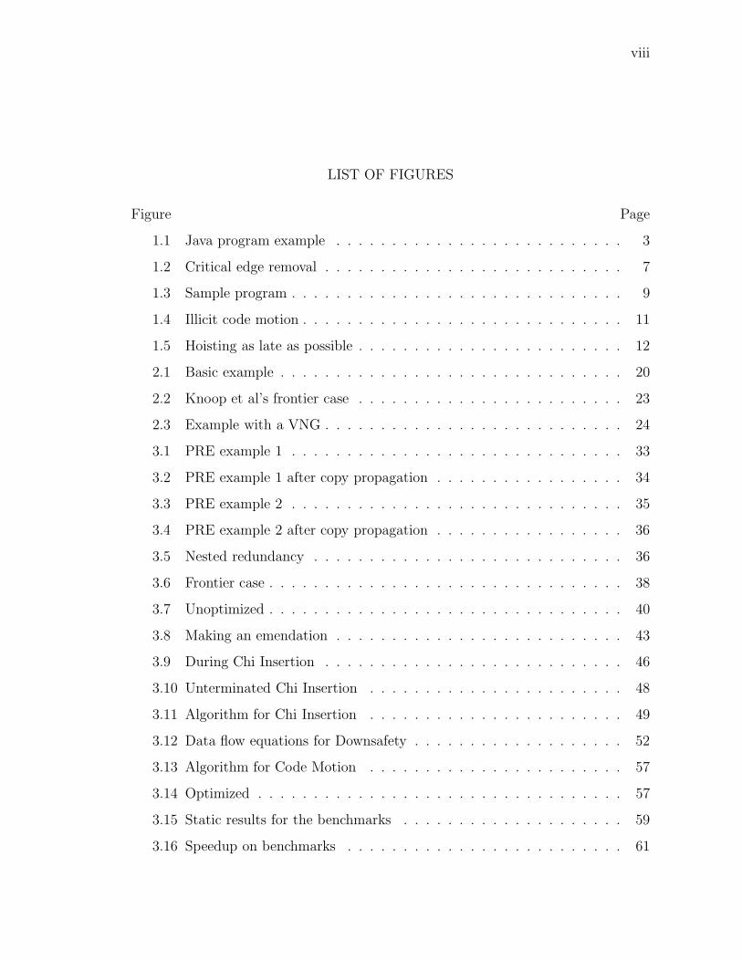
LIST OF FIGURES
Figure Page
1.1 Java program example . . . . . . . . . . . . . . . . . . . . . . . . . . 3
1.2 Critical edge removal . . . . . . . . . . . . . . . . . . . . . . . . . . . 7
1.3 Sample program . . . . . . . . . . . . . . . . . . . . . . . . . . . . . . 9
1.4 Illicit code motion . . . . . . . . . . . . . . . . . . . . . . . . . . . . . 11
1.5 Hoisting as late as possible . . . . . . . . . . . . . . . . . . . . . . . . 12
2.1 Basic example . . . . . . . . . . . . . . . . . . . . . . . . . . . . . . . 20
2.2 Knoop et al’s frontier case . . . . . . . . . . . . . . . . . . . . . . . . 23
2.3 Example with a VNG . . . . . . . . . . . . . . . . . . . . . . . . . . . 24
3.1 PRE example 1 . . . . . . . . . . . . . . . . . . . . . . . . . . . . . . 33
3.2 PRE example 1 after copy propagation . . . . . . . . . . . . . . . . . 34
3.3 PRE example 2 . . . . . . . . . . . . . . . . . . . . . . . . . . . . . . 35
3.4 PRE example 2 after copy propagation . . . . . . . . . . . . . . . . . 36
3.5 Nested redundancy . . . . . . . . . . . . . . . . . . . . . . . . . . . . 36
3.6 Frontier case . . . . . . . . . . . . . . . . . . . . . . . . . . . . . . . . 38
3.7 Unoptimized . . . . . . . . . . . . . . . . . . . . . . . . . . . . . . . . 40
3.8 Making an emendation . . . . . . . . . . . . . . . . . . . . . . . . . . 43
3.9 During Chi Insertion . . . . . . . . . . . . . . . . . . . . . . . . . . . 46
3.10 Unterminated Chi Insertion . . . . . . . . . . . . . . . . . . . . . . . 48
3.11 Algorithm for Chi Insertion . . . . . . . . . . . . . . . . . . . . . . . 49
3.12 Data flow equations for Downsafety . . . . . . . . . . . . . . . . . . . 52
3.13 Algorithm for Code Motion . . . . . . . . . . . . . . . . . . . . . . . 57
3.14 Optimized . . . . . . . . . . . . . . . . . . . . . . . . . . . . . . . . . 57
3.15 Static results for the benchmarks . . . . . . . . . . . . . . . . . . . . 59
3.16 Speedup on benchmarks . . . . . . . . . . . . . . . . . . . . . . . . . 61
ix
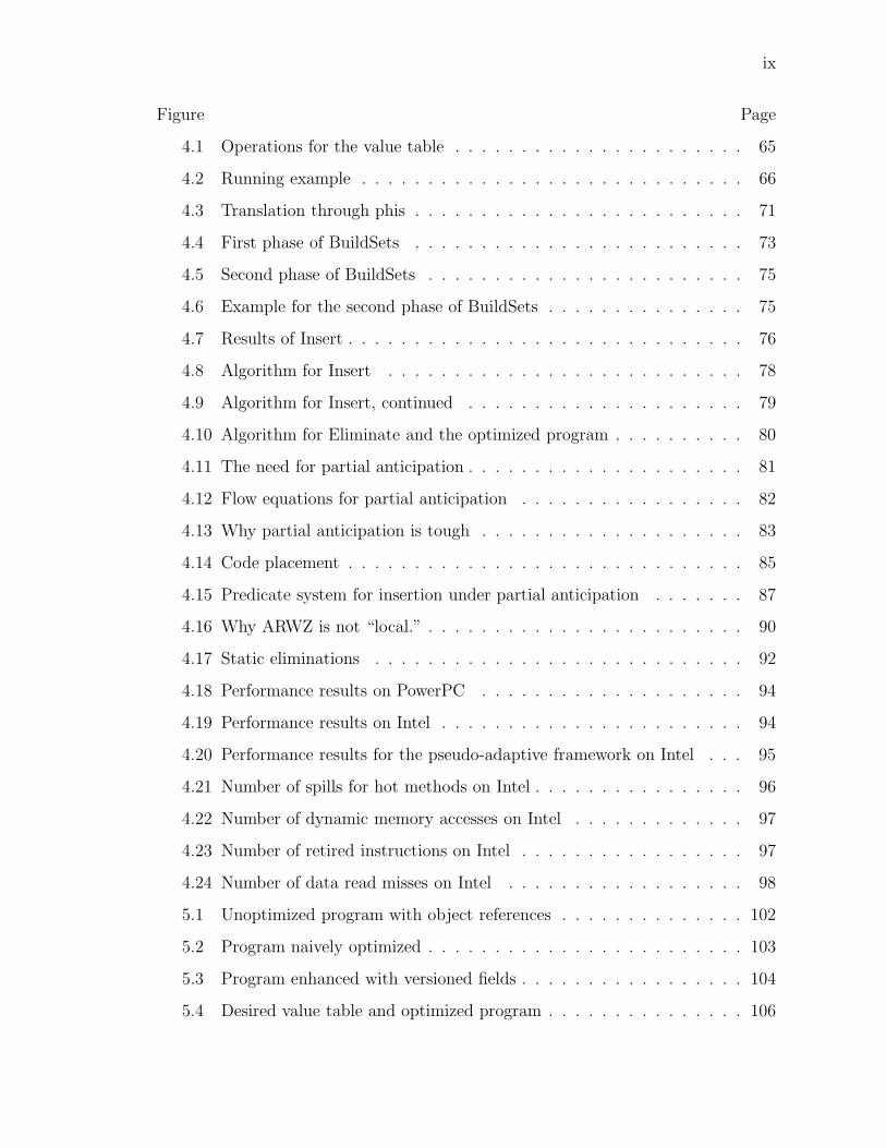
Figure Page
4.1 Operations for the value table . . . . . . . . . . . . . . . . . . . . . . 65
4.2 Running example . . . . . . . . . . . . . . . . . . . . . . . . . . . . . 66
4.3 Translation through phis . . . . . . . . . . . . . . . . . . . . . . . . . 71
4.4 First phase of BuildSets . . . . . . . . . . . . . . . . . . . . . . . . . 73
4.5 Second phase of BuildSets . . . . . . . . . . . . . . . . . . . . . . . . 75
4.6 Example for the second phase of BuildSets . . . . . . . . . . . . . . . 75
4.7 Results of Insert . . . . . . . . . . . . . . . . . . . . . . . . . . . . . . 76
4.8 Algorithm for Insert . . . . . . . . . . . . . . . . . . . . . . . . . . . 78
4.9 Algorithm for Insert, continued . . . . . . . . . . . . . . . . . . . . . 79
4.10 Algorithm for Eliminate and the optimized program . . . . . . . . . . 80
4.11 The need for partial anticipation . . . . . . . . . . . . . . . . . . . . . 81
4.12 Flow equations for partial anticipation . . . . . . . . . . . . . . . . . 82
4.13 Why partial anticipation is tough . . . . . . . . . . . . . . . . . . . . 83
4.14 Code placement . . . . . . . . . . . . . . . . . . . . . . . . . . . . . . 85
4.15 Predicate system for insertion under partial anticipation . . . . . . . 87
4.16 Why ARWZ is not “local.” . . . . . . . . . . . . . . . . . . . . . . . . 90
4.17 Static eliminations . . . . . . . . . . . . . . . . . . . . . . . . . . . . 92
4.18 Performance results on PowerPC . . . . . . . . . . . . . . . . . . . . 94
4.19 Performance results on Intel . . . . . . . . . . . . . . . . . . . . . . . 94
4.20 Performance results for the pseudo-adaptive framework on Intel . . . 95
4.21 Number of spills for hot methods on Intel . . . . . . . . . . . . . . . . 96
4.22 Number of dynamic memory accesses on Intel . . . . . . . . . . . . . 97
4.23 Number of retired instructions on Intel . . . . . . . . . . . . . . . . . 97
4.24 Number of data read misses on Intel . . . . . . . . . . . . . . . . . . 98
5.1 Unoptimized program with object references . . . . . . . . . . . . . . 102
5.2 Program naively optimized . . . . . . . . . . . . . . . . . . . . . . . . 103
5.3 Program enhanced with versioned fields . . . . . . . . . . . . . . . . . 104
5.4 Desired value table and optimized program . . . . . . . . . . . . . . . 106

x
Figure Page
5.5 Program in Extended Array SSA form . . . . . . . . . . . . . . . . . 108
5.6 Lattice equations and solutions for our example . . . . . . . . . . . . 110
5.7 Optimized by Fink et al’s load elimination . . . . . . . . . . . . . . . 111
5.8 Psi illustrated . . . . . . . . . . . . . . . . . . . . . . . . . . . . . . . 113
5.9 Illustration of use phi . . . . . . . . . . . . . . . . . . . . . . . . . . . 114
5.10 Illustration for control phis . . . . . . . . . . . . . . . . . . . . . . . . 114
5.11 Need for insertablility on all preds . . . . . . . . . . . . . . . . . . . . 116
5.12 Source example and equations from Fink et al . . . . . . . . . . . . . 117
5.13 Equations from our algorithm with optimized version . . . . . . . . . 117
5.14 Source example and equations from Fink et al . . . . . . . . . . . . . 118
5.15 Equations from our algorithm with optimized version . . . . . . . . . 118
5.16 Static eliminations . . . . . . . . . . . . . . . . . . . . . . . . . . . . 120
5.17 Performance results . . . . . . . . . . . . . . . . . . . . . . . . . . . . 121
5.18 Performance results for the pseudo-adaptive framework . . . . . . . . 121
5.19 Number of spills for hot methods . . . . . . . . . . . . . . . . . . . . 122
5.20 Number of dynamic memory accesses . . . . . . . . . . . . . . . . . . 123
5.21 Number of retired instructions . . . . . . . . . . . . . . . . . . . . . 124
5.22 Number of data read misses . . . . . . . . . . . . . . . . . . . . . . . 124
6.1 Example using Click’s “sea of nodes.” . . . . . . . . . . . . . . . . . . 129
xi
ABSTRACT
VanDrunen, Thomas John . Ph.D., Purdue University, August, 2004. PartialRedundancy Elimination for Global Value Numbering . Major Professor: AntonyL Hosking.
Partial redundancy elimination (PRE) is a program transformation that removes
operations that are redundant on some execution paths, but not all. Such a transfor-
mation requires the partially redundant operation to be hoisted to earlier program
points where the operation’s value was not previously available. Most well-known
PRE techniques look at the lexical similarities between operations.
Global value numbering (GVN) is a program analysis that categorizes expressions
in the program that compute the same static value. This information can be used to
remove redundant computations. However, most widely-implemented GVN analyses
and related transformations remove only computations that are fully redundant.
This dissertation presents new algorithms to remove partially redundant compu-
tations in a value-based view of the program. This makes a hybrid of PRE and GVN.
The algorithms should be simple and practical enough to be implemented easily as
optimization phases in a compiler. As far as possible, they should also to show true
performance improvements on realistic benchmarks.
The three algorithms presented here are: ASSAPRE, a PRE algorithm for pro-
grams in a form useful for GVN; GVNPRE, the hybrid algorithm for value-based
PRE; and LEPRE, an approximate PRE technique for object and array loads.

xii

1
1 INTRODUCTION
“You look a little shy; let me introduce you to that leg of mutton,” said the Red Queen.“Alice – Mutton; Mutton – Alice.” The leg of mutton got up in the dish and made alittle bow to Alice; and Alice returned the bow, not knowing whether to be frightenedor amused.“May I give you a slice?” she said, taking up the knife and fork, and looking from oneQueen to the other.“Certainly not,” the Red Queen, very decidedly: “it isn’t etiquette to cut any one you’vebeen introduced to.”
—Lewis Carroll, Alice through the Looking Glass
1.1 The thesis
1.1.1 General problem
A programming language is a system of expressing instructions for a real or theo-
retical machine which automates computation or some other task modeled by com-
putation. Viewed this broadly, programming languages include things as diverse as
the lambda calculus and the hole patterns in the punch cards of a Jacquard loom.
The former is a minimalist language that can encode anything computable in the
Church-Turing model of computation. The latter is of historic significance as the
first use of instructions stored in some form of memory to control the operation of
the machine.
Most modern computers interpret simple languages made up of binary-encoded
instructions that move information in memory, send information to devices, and
perform basic logical and arithmetic operations on the information. A non-trivial
computer program requires millions of such instructions. A language like this is
called a machine language.
As computing developed, it became evident that it was impractical for humans to
compose programs in machine languages. This prompted the invention of high-level
languages in which computational tasks could be described unambiguously but also
for which humans could be trained easily and in which programs could be composed

2
quickly. Since computers understand only machine languages, programs written in
a high-level language must be translated to a machine language.
In order to automate the process of translation from high-level languages to ma-
chine languages, programmers began composing computer programs whose purpose
was reading in other programs and translating them from one language (the source)
to another (the target). A computer program that translates computer programs is
called a compiler. A compiler is divided into three parts: a front-end, which lexi-
cally analyzes and parses the source program; a middle, which performs analyses and
transformations on the program for things like error checking or making improve-
ments; and a back-end, which emits the target program. Of course, each compilation
phase must represent the program in computer memory; a form of the program used
internally by the compiler is called an intermediate representation (IR). Two desir-
able properties of an IR are language independence and machine independence; that
is, programs in (nearly) any source high-level language can be represented by it, and
it can represent a program bound for (nearly) any target machine language.
A fundamental goal of computer science across its sub-disciplines is making com-
putational tasks faster. Naturally, a well-constructed compiler should produce target
programs that are as efficient as possible. The process of transforming a program for
better performance is called optimization. Optimization may happen at any phase
of the compiler, but much research has focused on mid-compiler optimizations since
they are widely applicable for languages and machine architectures.
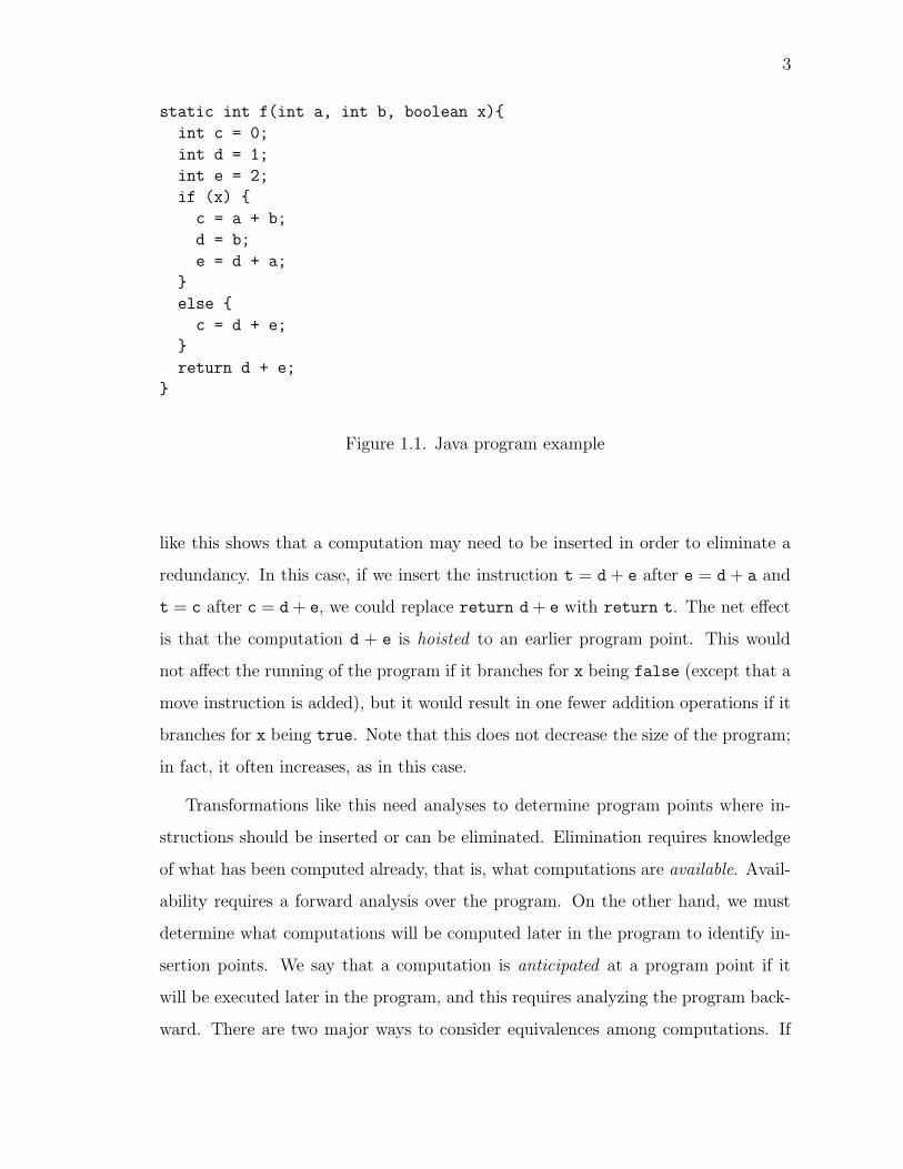
A common form of inefficiency in a program is redundancy, when identical or
equivalent tasks are performed twice. Consider the program fragment in Figure
1.1 written as a Java method: The computation d + a is redundant because it is
equivalent to the previous computation a+b. It would be more efficient to eliminate
that instruction. A more interesting case is the computation d+ e at the end of the
method. It is redundant if variable x is false and the second branch is taken, but
it is not redundant otherwise. If a computation is redundant on at least one but
not all traces of the program to that point, it is partially redundant. An example
3
static int f(int a, int b, boolean x)
int c = 0;
int d = 1;
int e = 2;
if (x)
c = a + b;
d = b;
e = d + a;
else
c = d + e;
return d + e;
Figure 1.1. Java program example
like this shows that a computation may need to be inserted in order to eliminate a
redundancy. In this case, if we insert the instruction t = d + e after e = d + a and
t = c after c = d + e, we could replace return d + e with return t. The net effect
is that the computation d + e is hoisted to an earlier program point. This would
not affect the running of the program if it branches for x being false (except that a
move instruction is added), but it would result in one fewer addition operations if it
branches for x being true. Note that this does not decrease the size of the program;
in fact, it often increases, as in this case.
Transformations like this need analyses to determine program points where in-
structions should be inserted or can be eliminated. Elimination requires knowledge
of what has been computed already, that is, what computations are available. Avail-
ability requires a forward analysis over the program. On the other hand, we must
determine what computations will be computed later in the program to identify in-
sertion points. We say that a computation is anticipated at a program point if it
will be executed later in the program, and this requires analyzing the program back-
ward. There are two major ways to consider equivalences among computations. If

4
two computations match exactly, including with respect to variable names, they are
lexically equivalent, as in the case of the two computations of d + e in our example.
Note, however, that even though a + b and d + a are not lexically equivalent, they
still compute the same value on any run of the program. This is an example of a
value equivalence. Analyses that consider value equivalences are stronger than those
that restrict themselves to lexical equivalences.
Previous work on this problem has fallen typically into two categories. Global
value numbering (GVN) analyzes programs to group expressions into classes, all of
which have the same value in a static view of the program. Partial redundancy
elimination (PRE) hoists computations to make partially redundant computations
fully redundant and thus removable.
1.1.2 Thesis statement
This dissertation concerns the removal of value-equivalent computations. By
presenting algorithms to this end, it seeks to demonstrate that
Practical, complete, and effective analyses for availability and anticipa-
tion allow transformations to remove full and partial value-equivalent
redundancies.
The algorithms presented here are practical in that they can be implemented
simply, incorporate easily into the optimization sequence of existing compilers, have
a reasonable cost, and represent an advancement over previous work in this area from
a software engineering perspective. They are complete in that they subsume other
algorithms with similar goals. They are effective in that they produce a performance
gain on some benchmarks. Finally, they consider not only lexically equivalent but
also value equivalent computations and remove not only full redundancies but also
partial redundancies.
In particular, we present three algorithms. The first is a PRE algorithm for an
IR property that is particularly useful for GVN. The second is a complete hybrid of

5
PRE and GVN. The third uses GVN to perform PRE on object and array references.
An additional contribution of this dissertation is the framework we use to discuss
programs and values for the purpose of optimizing analyses and transformations.
1.1.3 Outline
The remainder of this chapter explains preliminary matters relevant to all parts
of the dissertation: definitions for the IR and other details of our framework (Section
1.2.1), the cost model and standards we use to make claims of our algorithms’ worth
(Section 1.2.2), an overview of our experimental infrastructure (Section 1.2.3), and
a list of prior publications of the material presented here (Section 1.2.4). Chapter 2
traces the development of other approaches to this and similar problems. As implied
earlier, there are two major strains in the evolution, motivating the hybrid approach
which is the cornerstone of this dissertation.
Chapter 3 presents the ASSAPRE algorithm. Chow, Kennedy, et al introduced
SSAPRE [1, 2], an algorithm for PRE on IRs with a property called static sin-
gle assignment (SSA) form. We critique this algorithm in three areas. First, it is
fundamentally weak in that it is completely lexical in its outlook and ignores re-
dundancies involving secondary effects. Second, it actually makes requirements on
the IR that are more strict than SSA, as it is usually understood, and if applied
to a non-conforming program will perform erroneous transformations. Finally, it is
difficult to understand and implement. ASSAPRE is an improvement in these areas.
It reduces lexical restrictions on the expressions it considers, and it uses an antici-
pation analysis. Since SSA is useful for GVN, this algorithm illuminates how PRE,
which is typically lexical, can be extended for use with GVN, thereby considering
values-based equivalence.
Chapter 4 presents the GVNPRE algorithm. This is the chief contribution of
the dissertation and is a novel hybrid of earlier GVN and PRE approaches. It uses a
clean way of partitioning expressions into values that is an extension of a simple hash-
6
based GVN, uses a system of flow equations to calculate availability and anticipation
and to determine insertion points, and removes full and partial redundancies.
Chapter 5 presents the LEPRE algorithm. GVNPRE considers only scalar op-
erations, not, for example, loads from objects and arrays. We show that it is im-
possible to extend GVNPRE to cover loads completely. Fink et al. introduced an
algorithm for eliminating loads that are fully redundant [3]. Although not itself a
GVN scheme, it relies on GVN as input to its analysis. However, that algorithm
does not consider partial redundancies. As an approximate solution to the problem
of extending GVNPRE for loads, we extend Fink et al’s algorithm to use GVNPRE’s
analysis for doing PRE. We also sketch a different approach to cross-breeding GVN
and PRE that would be more amenable to the removal of loads.
We compare each algorithm to related approaches, describe an implementation,
and report on static and performance results. Chapter 6 concludes by considering
future work in this area.
1.2 Preliminaries
1.2.1 IR definitions and assumptions
We assume input programs represented as control flow graphs (CFGs) over basic
blocks [4]. A basic block is a code segment that has no unconditional jump or
conditional branch statements except for possibly the last statement, and none of its
statements, except for possibly the first, is a target of any jump or branch statement.
A CFG is a graph representation of a procedure that has basic blocks for nodes and
whose edges represent the possible execution paths determined by jump and branch
statements. Blocks are identified by numbers; paths in the graph (including edges)
are identified by a parenthesized list of block numbers. We define succ(b) to be the set
of successors to basic block b in the CFG, and similarly pred(b) the set of predecessors.
(When these sets contain only one element, we use this notation to stand for that
element for convenience.) We also define dom(b) to be the dominator of b, the nearest

7
(a) Critical edge in bold (b) Critical edge replaced by landing pad
Figure 1.2. Critical edge removal
block that dominates b. This relationship can be modeled by a dominator tree,
which we assume to be constructed before the performing of our algorithms [4]. The
dominance frontier of a basic block is the set of blocks that are not dominated by that
block but have a predecessor that is [5]. We assume that all critical edges—edges from
blocks with more than one successor to blocks with more than one predecessor [6]—
have been removed from the CFG by inserting an empty block between the two blocks
connected by the critical edge, as illustrated in Figure 1.2. Formally, this property
means that if |succ(b)| > 1 then ∀b′ ∈ succ(b), |pred(b′)| = 1 and if |pred(b)| > 1 then
∀b′ ∈ pred(b), |succ(b′)| = 1. This provides a landing pad for hoisting.
Figure 1.3(a) shows the sample program from Figure 1.1 as a CFG, and Figure
1.3(b) shows the optimized version. Note that we do not include branch instructions
in the CFG illustrations.
Static single assignment (SSA) form is an intermediate representation property
such that each variable—whether representing a source-level variable chosen by the
programmer or a temporary generated by the compiler—has exactly one definition
point [5, 6]. Even though definitions in reentrant code may execute many times,
statically each SSA variable is assigned exactly once. If several distinct assignments
to a variable occur in the source program, the building of SSA form splits that
variable into distinct versions, one for each definition. In basic blocks where execution
paths merge (such as block 4 in our example) the consequent merging of variables

8
is represented by a phi function. Phi functions occur only in instructions at the
beginning of a basic block (before all non-phi instructions) and have the same number
of operands as the block has predecessors in the CFG, each operand corresponding
to one of the predecessors. The result of a phi function is the value of the operand
associated with the predecessor from which control has come. A phi function is
an abstraction for moves among temporaries that would occur at the end of each
predecessor. SSA form does not allow such explicit moves since all would define the
same variable. SSA makes it easy to identify the live ranges of variable assignments
and hence which lexically equivalent expressions are also semantically equivalent. On
the other hand, SSA complicates hoisting since any operand defined by a merge of
variable versions must have the earlier version back-substituted. Figure 1.3(c) shows
the sample program in SSA form, where we name SSA variables using subscripts on
the names of the source-level variables from which they come. In some examples, we
ignore the relationship with pre-SSA variable names and consider all SSA variables
to be independent temporaries.
We now formally define the language for our examples (this excludes jumps and
branches, which for our purposes are modeled by the graph itself):
k ::= t | t1 op t2 (| gf x t) Operations
p ::= φ(t∗) Phis
γ ::= k | p | • Right-hand terms
i ::= t← γ (| pf x t1 t2) Instructions
b ::= i∗ Basic blocks
Note that basic blocks are considered vectors of instructions. The symbol • stands
for any operation which we are not considering for optimization; it is considered to
be a black box which produces a result. The meta-variable t ranges over (SSA)
variables. Because of SSA form, no variable is reassigned, and a variable’s scope is
implicitly all program points dominated by its definition. For simplicity, we do not
include constants in the grammar, though they appear in some examples; constants

9
e ← d+ a
d← b
c← a+ b
r ← d+ e
c← d+ e
e ← 2
d← 1
c← 0
1
4
32
c← 0
t← c
c← d+ e
t← d+ e
e← c
d← b
c← a+ b
r ← t
e← 2
d← 1
1
4
32
(a) Original (b) Optimized
e3 ← φ(e2, e1)
d3 ← φ(d2, d1)
c4 ← φ(c2, c3)
e2 ← d2 + a1
d2 ← b1
c2 ← a1 + b1
r ← d3 + e3
c3 ← d1 + e1
e1 ← 2
d1 ← 1
c1 ← 0
1
4
32
(c) In SSA form
Figure 1.3. Sample program
10
may be treated as globally-defined temporaries. We use the term operation instead
of expression to leave room for a more specialized notion of expressions in Chapter
4. We let op range over operators, such as arithmetic or logical operators. gf x t
is a getfield operation, that is, one that retrieves the value of field x of the object
to which t points. x ranges over field names. pf x t1 t2 is a putfield operation,
setting field x of the object pointed to by t1 to hold the value of t2. The productions
involving gf and pf are bracketed because we use them only at certain points in
this dissertation; otherwise getfields are replaced with • and putfields are ignored.
For simplicity, the only types we recognize are integer and object, and we assume
all programs type correctly, including that getfields and putfields use only legitimate
fields.
1.2.2 Cost model and goals
The proof of an optimization’s worth is real performance gain when applied to
real-world benchmarks. That said, theoretical cost models are useful in evaluating
optimizations abstractly, apart from a specific language or architecture. We consider
each operation (t1 op t2 or gf x t) to cost one unit. Moves (such as t1 ← t2) are
free. Our goal is to reduce the number of units on traces of the input program. This
implies we may freely generate new temporaries and insert new moves in our effort
to reduce other instructions. We consider this to be a realistic cost model because
move instructions and extra temporaries largely can be cleaned up by good register
allocation. Though it may seem naıve to give arithmetic operations and getfields
equal cost when, for any realistic architecture, getfields are much more expensive
(an important point in our experimental evaluation), we still feel justified in treating
them as though equal because at no time in the algorithms presented would one be
substituted for another; that is, one never needs to choose between an arithmetic
operation and a getfield.

11
EXIT
54
d← a / b3
1 2
b2← •b1 ←
c← a / b1
3
b3 ← φ(b1, b2)
EXIT
c3 ← φ(c1, c2)
c2 ← a / b2
54
c4 ← c3
1 2
b2← •b1 ←
c1 ← a / b1
3
b3 ← φ(b1, b2)
(a) Unoptimized (b) Incorrectly “optimized”
Figure 1.4. Illicit code motion
Our algorithms must be Hippocratic in that they should do no harm. Generally,
a PRE hoist will improve one path while making no change on another. What is not
acceptable is a transformation that improves one path while making another path
worse. Consider the example in Figure 1.4(a). The operation d← a / b3 is partially
redundant in block 4, since it already has been computed in path (1,3,4) but not
in path (2,3,4). Hoisting the computation to block 2 as shown in 1.4(b) removes
the block 4 computation and improves the path (1,3,4) without changing (2,3,4).
However, this lengthens the path (2,3,5). Not only does this defy optimality, but
if the hoisted instruction throws an exception (in our case, if b2 is zero), then the
transformation has changed the behavior of the program by introducing an exception
where otherwise there was not one. This illustrates the need for anticipation analysis.
A hoist should be performed only for an expression that is anticipated on all paths
from that point to program exit.
One potential casualty of hoisting instructions is that it lengthens the live ranges
of variables, increasing register pressure and potentially harming performance. We
believe that since most hoists are fairly local and many modern architectures have

12
7
65
4
3
2
1
t3 ← t0 + t1
t2 ← t0 + t1
(a) Original
t2 ← t0 + t1
7
65
4
3
2
1
t3 ← t2
t5 ← φ(t0, t1)
t4 ← t0 + t1
7
65
4
3
2
1
t3 ← t5
t2 ← t0 + t1
(b) Early hoisting (c) Late hoisting
Figure 1.5. Hoisting as late as possible
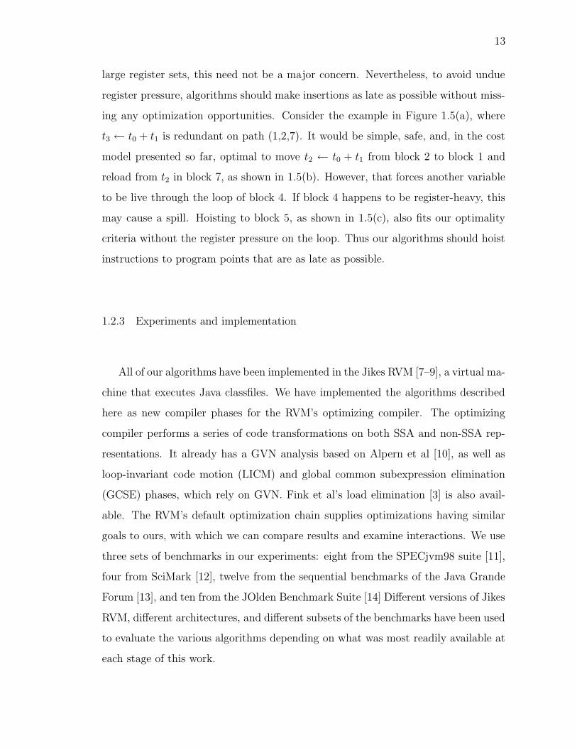
13
large register sets, this need not be a major concern. Nevertheless, to avoid undue
register pressure, algorithms should make insertions as late as possible without miss-
ing any optimization opportunities. Consider the example in Figure 1.5(a), where
t3 ← t0 + t1 is redundant on path (1,2,7). It would be simple, safe, and, in the cost
model presented so far, optimal to move t2 ← t0 + t1 from block 2 to block 1 and
reload from t2 in block 7, as shown in 1.5(b). However, that forces another variable
to be live through the loop of block 4. If block 4 happens to be register-heavy, this
may cause a spill. Hoisting to block 5, as shown in 1.5(c), also fits our optimality
criteria without the register pressure on the loop. Thus our algorithms should hoist
instructions to program points that are as late as possible.
1.2.3 Experiments and implementation
All of our algorithms have been implemented in the Jikes RVM [7–9], a virtual ma-
chine that executes Java classfiles. We have implemented the algorithms described
here as new compiler phases for the RVM’s optimizing compiler. The optimizing
compiler performs a series of code transformations on both SSA and non-SSA rep-
resentations. It already has a GVN analysis based on Alpern et al [10], as well as
loop-invariant code motion (LICM) and global common subexpression elimination
(GCSE) phases, which rely on GVN. Fink et al’s load elimination [3] is also avail-
able. The RVM’s default optimization chain supplies optimizations having similar
goals to ours, with which we can compare results and examine interactions. We use
three sets of benchmarks in our experiments: eight from the SPECjvm98 suite [11],
four from SciMark [12], twelve from the sequential benchmarks of the Java Grande
Forum [13], and ten from the JOlden Benchmark Suite [14] Different versions of Jikes
RVM, different architectures, and different subsets of the benchmarks have been used
to evaluate the various algorithms depending on what was most readily available at
each stage of this work.

14
1.2.4 Publications
The material in Chapter 3 is to appear in Software—Practice & Experience [15].
The material in Chapter 4 was presented at the Thirteenth International Confer-
ence on Compiler Construction in April 2004 [16], with more details given in an
accompanying technical report at Purdue University [17].
15
2 RELATED WORK
Infandum, regina, iubes renovare dolorem.
(You command me, queen, to recall unspeakable pain.)
—Virgil, The Aeneid, II, 3.
These are the generations of redundancy elimination. One of the earliest rec-
ognizable efforts related to our problem arose in the work of Cocke, in which he
identified our “aim to delete those computations which have been previously per-
formed, [and] when possible to move computations from their original positions to
less frequently executed regions,” proposed a flow analysis to determine if expres-
sions can be eliminated or moved, and explained a primitive form of critical edge
splitting [18,19]. Kildall, infamous for losing a crucial contract with IBM to a young
Bill Gates [20], outlined a generalized optimization technique which, parameterized
by an “optimizing function,” could be used for a variety of transformations on a
program as a CFG [21,22]; in this work, he foresaw GVN by proposing an optimiz-
ing function for common subexpression elimination that partitions expressions into
equivalence classes.
2.1 Partial redundancy elimination
PRE was invented by Morel and Renvoise [23, 24]. They identified partial re-
dundancy as a generalization of loop invariance and defined a set of properties to
determine appropriate transformations: transparency, true for an expression in a
block which does not modify its operands; availability, true for an expression in a
block which computes it and does not modify its operands after the final compu-
tation; anticipation (in situ, anticipability), true for an expression in a block that
computes it and does not modify its operands before the first computation; and in-
sert, true for an expression in a block where it is anticipated and also available in
16
at least one predecessor. Since these properties are computed per expression, the
algorithm is inherently lexical. Since they involve both availability and anticipation,
it is bidirectional. Drechsler and Stadel [25] and several others [26] modified the al-
gorithm to better handle subexpressions. Dhamdhere adapted the algorithm to have
more elimination opportunities by the splitting of critical edges [27] and to avoid
code motion that does not produce real redundancy elimination [28].
The epoch for PRE is Lazy Code Motion (LCM), invented by Knoop, Ruthing,
and Steffen [29, 30]. Its principle contribution is an algorithm that is provably opti-
mal but takes register pressure into account by hoisting expressions no earlier than
necessary. It uses four properties to determine hoisting and elimination of expres-
sions: downsafety, equivalent to anticipation; earliest, true for an expression and a
block if that expression is downsafe at the block but not on any path from the start
to that block; latest, true for an expression and a block if the expression is optimally
placed there but would not be optimally placed on any path from that block to
the exit; and isolated, true for an expression and a block if that expression, placed
at that block, would reach no other occurrence of that expression (that is, without
reassignment of its operands) to program exit. Identifying these properties allows
the typical bi-directional analysis to be broken down into uni-directional components
(something foreseen by Dhamdhere et al [31]), which the researchers claimed to be
more efficient. Drechsler and Stadel contributed to this work by showing how it
could be used on full-sized basic blocks (as opposed to blocks of only one instruction
as in the original presentation [29]) and by simplifying the flow equations [32]. As
with original PRE, this approach is expression-based and thus lexical.
The world that came after LCM saw numerous minor PRE projects. Wolfe
showed that the elimination of critical edges was all that is necessary to achieve uni-
directionality as in LCM [33]; his PRE, however, did not attempt to minimize register
pressure. Briggs and Cooper did a fascinating study on making PRE more effective
[34]. They identified PRE’s reliance on lexical equivalence as a major handicap; its
inability to rearrange subexpressions also limits the redundant computations it can

17
recognize. They showed that by first propagating expressions forward to their uses
(the opposite of what optimizations like common subexpression elimination and PRE
do), sorting and reassociating the expressions, and renaming them using information
gained from GVN, many more optimization opportunities are exposed for PRE.
Note that this essentially uses GVN to enhance PRE, yet it is not a hybrid like the
algorithm in Chapter 4 because it uses GVN in enabling transformations prior to
PRE rather than forming a unified algorithm that performs both. Paleri et al claimed
to have simplified LCM by incorporating the notion of safety (being either available
or anticipated) into the definitions of partial availability and partial anticipation
and adjusting the flow equations appropriately [35]. We noted earlier that PRE
increases code size; LCM’s own inventors developed a variant that takes code growth
as well as register pressure into consideration in deciding among possible optimal
transformations [36]. Hosking et al applied PRE to pointer dereferencing operations,
which they termed “access paths” [37]. The most important development for the
purposes of this dissertation is SSAPRE, designed by Chow, Kennedy et al to take
programs in SSA form as input and to preserve SSA across the transformation [1,2];
this algorithm will be discussed in detail in Chapter 3.
2.2 Alpern-Rosen-Wegman-Zadeck global value numbering
Identifying the origin of GVN is difficult, but it is clear at least that one GVN
heritage was founded by two papers simultaneously published by Alpern, Rosen,
Wegman, and Zadeck [6, 10]. One paper described how expressions can be parti-
tioned into congruence classes globally, as opposed to merely in view of a single
basic block or another restricted program fragment [10]. Congruence is a conserva-
tive approximation to equivalence, a property undecidable at compile-time, that a
set of expressions all have the same value as each other at run-time. This algorithm
initially makes the optimistic assumption that large classes of expressions are congru-
ent and refines the partitioning by splitting congruence classes until reaching a fixed

18
point. The other paper did not outline a specific global value numbering analysis,
but simply used SSA and an analysis of trivial moves to make a broader application
of what otherwise would be a lexical scheme for eliminating redundancy, including
partial [6]. It introduced a system of expression ranks, where a nested expression has
a lower rank than a later expression in which its result is used, which the algorithm
uses to cover secondary effects, opportunities which a transformation makes for more
optimization. (This concept of ranks was also used by Briggs and Cooper, discussed
above [34], and it removes the need to maintain the order of computations in a ba-
sic block, anticipating Click’s “sea of nodes” IR [38].) The algorithm maintains a
local computation table for each basic block containing the expressions that occur
in the block. The movable computation table for each edge contains the expressions
anticipated at the beginning of the block to which the edge leads. These are used to
determine where to place hoists. After hoisting, the algorithm searches backwards
from a computation to find an earlier occurrence and, if one is found, eliminates the
redundant computation.
A side contribution of these papers is that they gave the first (to our knowl-
edge) published description of SSA and an algorithm to build it. One of the papers
demonstrated many advantages of SSA [6], and has inspired work on more efficient
algorithms for SSA construction [5], the relationship between SSA and functional
programming [39], and related IRs [3, 38, 40].
This ARWZ GVN launched a line of research in GVN, largely done at Rice
University. Not all the algorithms produced by this heritage follow the ARWZ
schemes—most, in fact, present themselves as alternatives. The unifying feature
is the mind-set of what GVN should be: a method for grouping expressions by static
value so that recomputations of available values can be eliminated. Click extended
GVN to recognize algebraic identities (for example, a+a has the same value as a∗2)
and observed its interaction with constant copy propagation [41,42]. He also devised
an alternate, hashing GVN algorithm and combined it with a heuristic for pulling
computations out of loops to approximate loop invariant code motion and compete
19
with PRE [43]. The clearest description of hash-based GVN comes from Briggs,
Cooper, and Simpson [44,45]. A hash table associates the name of an expression—a
constant, a variable, or a computation—to a congruence class or value number. SSA
guarantees that such an association is well defined (a variable always has the same
value) and permits a global view. An assignment asserts that two expressions are in
the same congruence class. If the hash table is built by walking over the dominator
tree (so all code that dominates a point is visited before that point), then for any
computation, we know that the operands have already been set in the hash table (ex-
cept possibly for constants, whose congruence class is obvious). Since this approach
is used in our GVN-PRE hybrid, we reserve the details for Chapter 4. Cooper and
Simpson identified another approach to GVN, called Strongly Connected Component
(SCC)- Based Value Numbering [45,46], which uses a hashtable but is flexible enough
to allow for congruence classes to be refined and use the SSA graph (a representation
of the relationship among SSA variables defined by the phis) instead of the CFG. In
Chapter 7 of his dissertation, Simpson described a use of GVN to improve the LCM
algorithm for PRE; the essence of this approach, which Simpson called Value-Driven
Code Motion, is to capture more precisely under what conditions the recomputation
of a subexpression kills the availability of an available expression [45]. In addition
to the work of the Rice University group, Gargi extended ARWZ GVN to perform
forward propagation and reassociation (as used by Briggs and Cooper [34]) and to
consider back edges in the SSA graph to discover more congruences.
How does this understanding of GVN compare with PRE? Based on what we have
surveyed so far, one might conclude that “PRE finds lexical congruences instead of
value congruences” [43] but finds them even when only partially redundant, whereas
GVN finds value congruences but can remove only full redundancies. This is the
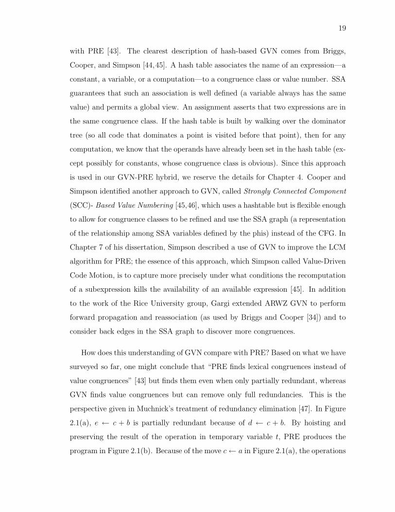
perspective given in Muchnick’s treatment of redundancy elimination [47]. In Figure
2.1(a), e ← c + b is partially redundant because of d ← c + b. By hoisting and
preserving the result of the operation in temporary variable t, PRE produces the
program in Figure 2.1(b). Because of the move c← a in Figure 2.1(a), the operations
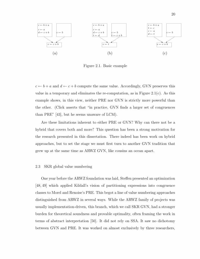
20
c← a
d← c+ b c← 5
c← b + a
e ← c+ b
c← a
d← c+ b c← 5
c← b + a
e ← t
t← d t← c+ b
c← 5
c← b + a
e← c+ b
d← t
c← a
t← c
(a) (b) (c)
Figure 2.1. Basic example
c← b+ a and d← c+ b compute the same value. Accordingly, GVN preserves this
value in a temporary and eliminates the re-computation, as in Figure 2.1(c). As this
example shows, in this view, neither PRE nor GVN is strictly more powerful than
the other. (Click asserts that “in practice, GVN finds a larger set of congruences
than PRE” [43], but he seems unaware of LCM).
Are these limitations inherent to either PRE or GVN? Why can there not be a
hybrid that covers both and more? This question has been a strong motivation for
the research presented in this dissertation. There indeed has been work on hybrid
approaches, but to set the stage we must first turn to another GVN tradition that
grew up at the same time as ARWZ GVN, like cousins an ocean apart.
2.3 SKR global value numbering
One year before the ARWZ foundation was laid, Steffen presented an optimization
[48, 49] which applied Kildall’s vision of partitioning expressions into congruence
classes to Morel and Renoise’s PRE. This begot a line of value numbering approaches
distinguished from ARWZ in several ways. While the ARWZ family of projects was
usually implementation-driven, this branch, which we call SKR GVN, had a stronger
burden for theoretical soundness and provable optimality, often framing the work in
terms of abstract interpretation [50]. It did not rely on SSA. It saw no dichotomy
between GVN and PRE. It was worked on almost exclusively by three researchers,

21
Steffen, Knoop, and Ruthing (the same heroes of LCM in PRE’s golden age [29,30]),
and while itself conscious of the ARWZ family, it was frustratingly overlooked by
its counterparts. A scan of the references in Ph.D. theses from the Rice University
group finds no citations of this work [42,45]; even work as late as Gargi’s cited only
one paper, and then only for a discussion of ARWZ [51,52].
The seminal paper notes that Morel and Renoise’s PRE can move computations,
but cannot recognize non-lexical equality, in both cases unlike Kildall [48]. It recasts
Kildall’s analysis as an abstract interpretation and proves it correct. Since SSA is
not used, variables can be redefined and hence expressions can change value, and so
the partitioning of expressions may be different at every program point. The paper
considers the state of the partitioning at the beginning and end of every basic block
(the pre- and post-partitions with respect to a block). The Value Flow Graph (VFG)
has the congruence classes of pre- and post-partitions as nodes and edges that repre-
sent value equivalence among congruence classes from different partitions as affected
by the assignments in a block or the join points in the CFG. A system of boolean
equations to determine maximally connected subgraphs of the VFG reveals optimal
computation points; from this code can be moved and the program optimized.
How does this compare with ARWZ and its seed? Steffen, with Knoop and
Ruthing, claimed that the VFG was superior to SSA because SSA algorithms are
optimal only for programs without loops and correct only for reducible CFGs [53].
However, it is worth noting that if SSA expressions are partitioned into global congru-
ence classes such as in a simple hash-based GVN, a graph representing the relevant
information of the VFG can be constructed merely by inspecting the phis. SKR also
introduces more trivial redefinitions than ARWZ [54], and its researchers also con-
ceded that its computational complexity, compared to ARWZ, was “probably one of
the major obstacles opposing to its widespread usage in program optimization” [52].
The researchers maintained, however, that SKR was more complete, general, and
amenable to theoretical reasoning.

22
What SKR lacked in practical acceptance, it compensated for by being a fruit-
ful sanctuary for contemplating the deeper truths of redundancy elimination. The
researchers’ experience with both PRE and GVN allowed them to make a lucid de-
scription of the state of then-current research [55]. All redundancy elimination that
involves hoisting hangs on the notion of safety, the property that a computation’s
value will be computed by every trace of the program passing that point. This prop-
erty is approximated by decomposition into availability (called upsafety in SKR)
and anticipation (downsafety); a computation is safe if it is either available or an-
ticipated. In a lexical (or syntactic) view, this “if” is really “if and only if,” that is,
the approximation is precise. However, Knoop et al showed that in a value-based
(in their terms, semantic) view, it is not. Consider the program in Figure 2.2 (taken
from Knoop et al [55] in substance but put into our framework). Is either a + b or
c3 +b safe at the beginning of block 3? a+b is available from block 2 but not block 1
and anticipated from block 4 but not block 5, and c3 +b is available from block 2 but
not block 1 and anticipated from block 5 but not block 4; our approximation would
say “no” to both. However, they indeed are safe because if control comes from block
2, they both will have been computed, and if control comes from block 1, they are the
same value and thus definitely will be computed later, whether control takes block
4 or block 5. Knoop et al call algorithms that use the approximation code motion,
whereas code placement refers to schemes, perhaps oracular, that find true safety.
Knoop et al considered examples like this the “frontier” for algorithms attempting
semantic code placement, and conjectured that, apart from algorithms that change
the structure of the CFG [56], “there does not exist a satisfactory solution to the
code placement problem” [55].
2.4 Bodık’s VNGPRE
This was the fullness of research at the advent of Bodık. In two papers presented
at about the same time, he and his co-authors answered the challenge of Knoop et

23
54
3
21
e2 ← c3 + bd2 ← a + b
d1 ← a + b
c3 ← φ(c1, c2)
e1 ← c2 + b
c1 ← a
54
3
21
t1 ← a + b
t3 ← φ(t1, e1)
t2 ← φ(t1, d1)
e2 ← t2d2 ← t2
d1 ← a + b
c3 ← φ(c1, c2)
e1 ← c2 + b
c1 ← a
(a) (b)
Figure 2.2. Knoop et al’s frontier case
al [57, 58]. One of the papers used CFG-restructuring for a practical and complete
PRE [58]. The other paper applied a series of analyses to a representation similar
to the VFG and performed a PRE that tore through the SKR frontier [57]. In this
framework, expressions are names of values. If the program is not in SSA, expres-
sions represent different values at different program points (where a “program point”
is recognized between each instruction, branch, and join). Bodık defined a structure
called the Value Name Graph (VNG) whose nodes are expression / program-point
pairs. The edges capture the flow of values from one name to another according to
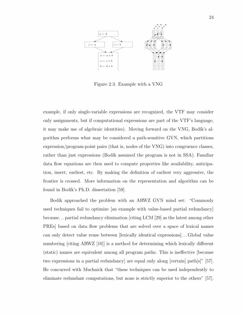
program control flow. Consider the program in Figure 2.3 with its VNG alongside.
For each program point (between each instruction, branch, and join) there are three
nodes, one for each of the expressions a + b, c + b, and d + b. Note that edges ex-
ist between nodes of the same expression unless there is a killing assignment to an
operand. Such assignments produce edges between lexically different expressions. A
path in such a graph is called a value thread. The edges (and therefore threads) are
built by performing backward substitution—that is, starting at the end of the pro-
gram and connecting threads based on the assignments at each instruction; see how
the assignment c← a substitutes a for c to sew c+b to a+b at the appropriate point.
The power of this back-substitution is determined by a parameterized Value Trans-
fer Function (VTF), which depends on the language of expressions recognized (for
24
b← d + b
c← c + b
a← a + b
c← 5c← a
a← d
c+
b
d+
b
a+
b
Figure 2.3. Example with a VNG
example, if only single-variable expressions are recognized, the VTF may consider
only assignments, but if computational expressions are part of the VTF’s language,
it may make use of algebraic identities). Moving forward on the VNG, Bodık’s al-
gorithm performs what may be considered a path-sensitive GVN, which partitions
expression/program-point pairs (that is, nodes of the VNG) into congruence classes,
rather than just expressions (Bodık assumed the program is not in SSA). Familiar
data flow equations are then used to compute properties like availability, anticipa-
tion, insert, earliest, etc. By making the definition of earliest very aggressive, the
frontier is crossed. More information on the representation and algorithm can be
found in Bodık’s Ph.D. dissertation [59].
Bodık approached the problem with an ARWZ GVN mind set: “Commonly
used techniques fail to optimize [an example with value-based partial redundancy]
because. . . partial redundancy elimination [citing LCM [29] as the latest among other
PREs] based on data flow problems that are solved over a space of lexical names
can only detect value reuse between [lexically identical expressions]. . . Global value
numbering [citing ARWZ [10]] is a method for determining which lexically different
(static) names are equivalent among all program paths. This is ineffective [because
two expressions in a partial redundancy] are equal only along [certain] path[s]” [57].
He concurred with Muchnick that “these techniques can be used independently to
eliminate redundant computations, but none is strictly superior to the others” [57].

25
Nevertheless, note that this representation is essentially Knoop et al’s VFG applied
to instructions rather than basic blocks; Knoop et al also make use of a backwards
substitution function δ, which is equivalent to the VTF [55]. This seems to have
been more prophetic than influential, as Bodık says, “Knoop, Ruthing, and Steffen
developed independently from us a representation called the Value Flow Graph” [57].
How do we evaluate Bodık’s work? The power of his representation and algorithm
is remarkable. Bodık himself conceded it produces significant register pressure [60].
Dhamdhere pointed out that its granularity to single instructions (as opposed to
basic blocks) makes it very complex conceptually [61]. Although Bodık backed up
his claims with an implementation [57,59], it is difficult to imagine a software engineer
picking up one his papers and incorporating it into an optimizing compiler, given
its complexity and memory demands. The research in this dissertation makes a
complete, value-based PRE accessible to all compilers, that they may observe the
goals Bodık made. We make comparisons to Bodık’s till the close of the dissertation.

26

27
3 ANTICIPATION-BASED PARTIAL REDUNDANCY ELIMINATION
Sergeant Hunter: You know what I would do if I were you?Pee-Wee: What?Sergeant Hunter: I’d retrace my steps.
—Pee-Wee’s Big Adventure
3.1 Introduction
In this chapter, we present a new algorithm for PRE in SSA. An earlier SSA-
based algorithm, SSAPRE, by Chow, Kennedy, et al [1, 2], is weak in several ways.
First, it makes stronger assumptions about the form of the program (particularly the
lives ranges of variables) than are true for the traditional definition of SSA. Other
SSA-based optimizations that are considered to preserve SSA may break these as-
sumptions; if these other optimizations are performed before SSAPRE, the result
may be incorrect. Moreover, the SSAPRE algorithm does not handle nested expres-
sions (secondary effects) or address the frontier identified by SKR [55], as Bodık’s
work does [57]. Finally, from a software engineering perspective, the earlier PRE
algorithm for SSA is difficult to understand and implement. In this chapter we will
describe SSAPRE and illustrate its shortcomings. Next, we present our main contri-
bution: a new algorithm for PRE that assumes and preserves SSA, called ASSAPRE.
It is structurally similar to, though simpler than, SSAPRE. The key difference is that
it discovers redundancy by searching backwards from later computations that can be
eliminated to earlier computations, rather than searching forward from early com-
putations to later. Our running example will demonstrate that our new algorithm
addresses the concerns about SSAPRE. Finally, we present performance results for
ASSAPRE.

28
3.2 SSAPRE
In this section, we explain the SSAPRE algorithm of Chow, Kennedy, et al.
[1, 2], giving part of the motivation for the present work. First, we summarize
the concepts and describe the algorithm’s phases with an example. Second, we
demonstrate weaknesses of the algorithm to show where improvements are necessary.
3.2.1 Summary
As mentioned before, one useful tool when arranging any set of optimizations is
a suitable, common program representation. If all optimizations use and preserve
the same IR properties, then the task of compiler construction is simplified, op-
timization phases are easily reordered or repeated, and expensive IR-rebuilding is
avoided. LCM, the most widely recognized PRE algorithm at the time SSAPRE was
presented, did not use SSA [29,30], and Briggs and Cooper [34] explicitly broke SSA
before performing PRE. The principle motivation for SSAPRE is to do PRE while
taking advantage of and maintaining SSA form.
We have already spoken of the distinction of lexical and value-based views of the
program. SSAPRE is lexical, but important to its notion of lexical equivalence is the
idea that variables that are different SSA versions of the same source-level variable
are still considered lexically the same. SSAPRE associates expressions that are
lexically equivalent when SSA versions are ignored. For example, a1 + b3 is lexically
equivalent to a2 + b7. We take a + b as the canonical expression and expressions
like a1 + b3 as versions of that canonical expression; lexically equivalent expressions
are assigned version numbers analogous to the version numbers of SSA variables. A
chi statement1 (or simply chi) merges versions of expressions at CFG merge points
just as phis merge variables. The chis can be thought of as potential phis for a
hypothetical temporary that may be used to save the result of the computation if
1In the original description of SSAPRE, Chow, Kennedy et al. [1, 2], chis are called Phis (distin-guished from phis by the capitalization) and denoted in code by the capital Greek letter Φ.

29
an opportunity for performing PRE is found. Just as a phi stores its result in a
new version of the variable, so chis are considered to represent a new version of an
expression. The operands of a chi (which correspond to incoming edges just as phi
operands do) are given the version of the expression that is available most recently
on the path they represent. If the expression is never computed along that path,
then there is no version available, and the chi operand is denoted by ⊥. Chis and chi
operands are also considered to be occurrences of the expression; expressions that
appear in the code are differentiated from them by the term real occurrences.
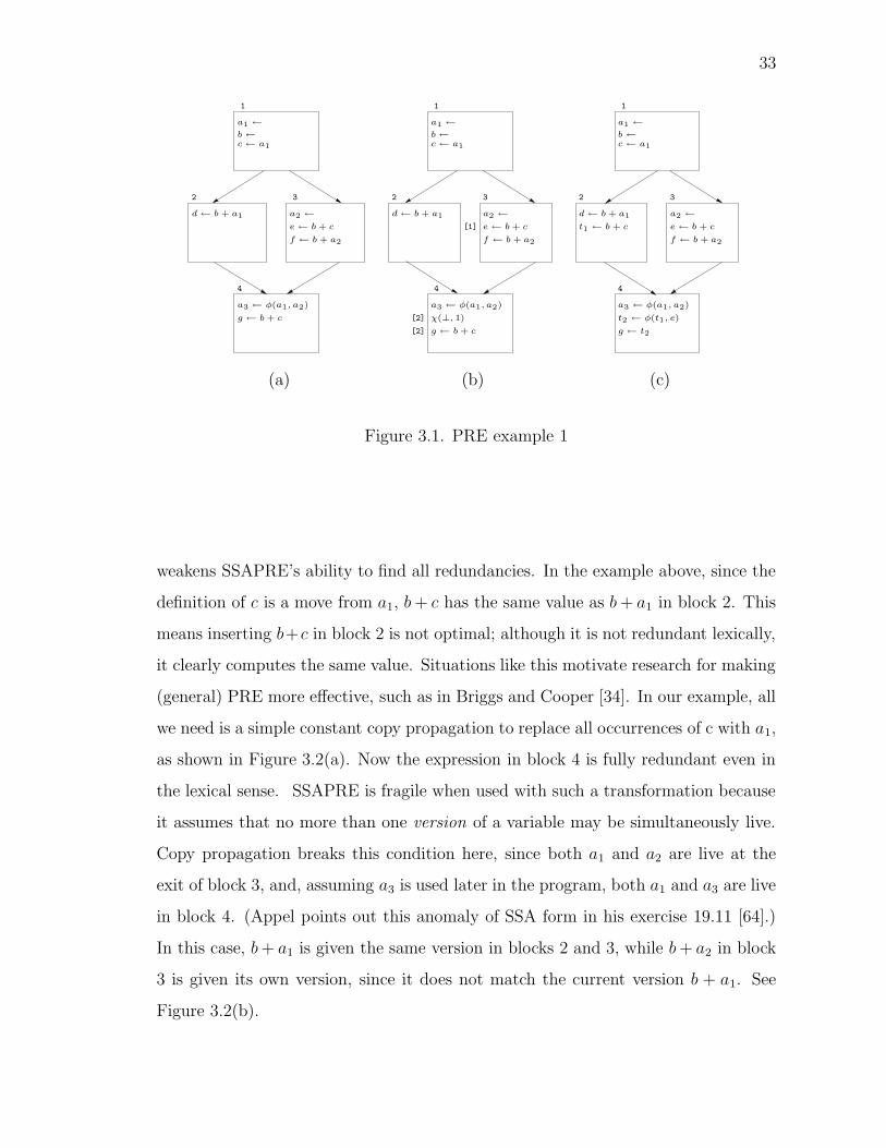
SSAPRE has six phases. We will discuss these while observing the example in
Figure 3.1. The unoptimized program is in Figure 3.1(a). The expression b + c in
block 4 is partially redundant because it is available along the right incoming edge.
1. Chi Insertion For any real occurrence of a canonical expression on which we
wish to perform SSAPRE, insert chis at blocks on the dominance frontier of
the block containing the real occurrence and at blocks dominated by that block
that have a phi for a variable in the canonical expression. (These insertions
are made if a chi for that canonical expression is not there already.) These chis
represent places that a version of an expression reaches but where it may not
be valid on all incoming edges and hence should be merged with the values
from the other edges. In our example, a chi is inserted at the beginning of
block 4 for canonical expression b+ c. Compare with the placement of phis in
Cytron et al’s SSA-building algorithm [5].
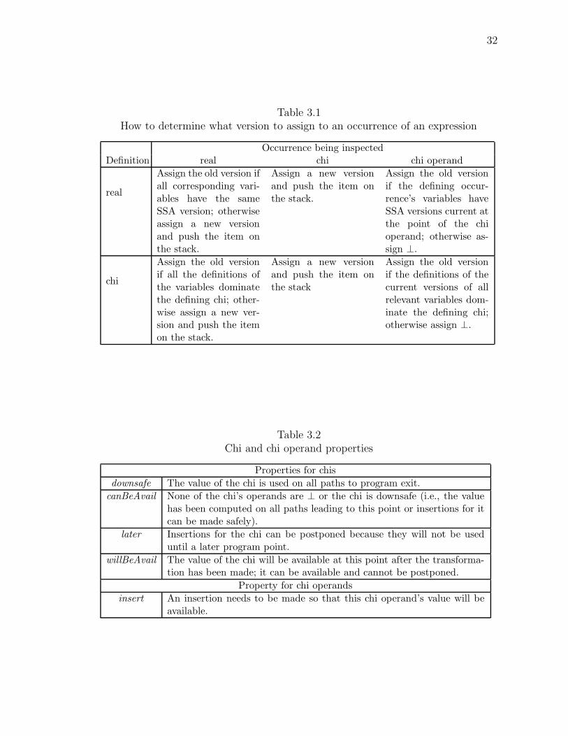
2. Rename Assign version numbers to all real expressions, chis, and chi operands.
This algorithm is similar to that for renaming SSA variables given in Cytron et
al [5]. While traversing the dominator tree of the CFG in preorder, maintain
a renaming stack for each canonical expression. The item at the top of the
stack is the defining occurrence of the current version of the expression. For
each block b in the traversal, inspect its chis, its real instructions, and its
corresponding chi operands in the chis of its successors, assigning a version

30
number to each. If an occurrence is given a new version number, push it on
the stack as the defining occurrence of the new version. When the processing
of all the blocks that b dominates is finished, pop the defining occurrences that
were added while processing block. Table 3.1 explains how to assign version
numbers for various types of occurrences depending on the defining occurrence
of the current version (this table is expanded from Table 1 of Chow, Kennedy
et al. [2], using delayed renaming). Note that chi operands cannot be defining
occurrences. Figure 3.1(b) shows our example after Rename. The occurrence
in block 3 is given the version 1. Since block 4 is on its dominance frontier,
a chi for this expression is placed there to merge the versions reaching that
point, and the right chi operand is given version 1. Since the expression is
unavailable from the left path, the corresponding chi operand is ⊥. The chi
itself is assigned version 2. Since that chi will be on top of the renaming stack
when b + c in block 4 is inspected and since the definitions of its variables
dominate the chi, it is also assigned version 2.
3. Downsafety Compute downsafety with another dominator tree preorder traver-
sal, maintaining a list of chis that have not been used on the current path.
When program exit is reached, mark the chis that are still unused (or used
only by operands to other chis that are not downsafe) as not downsafe. In our
example, the chi is clearly downsafe.
4. WillBeAvail Compute canBeAvail for each chi by considering whether it is
downsafe and, if it is not, whether its operands have versions that will be
available at that point. Compute later by setting it to false for all chis with
an operand that has a real use for its version or that is defined by a chi that
is not later. Compute willBeAvail by setting it to true for all chis for which
canBeAvail is true and later is false. Compute insert for each chi operand by
setting it to true for any operand in a chi for which willBeAvail is true and
either is ⊥ or is defined by a chi for which willBeAvail is false. Since the chi

31
in Figure 3.1(b) is downsafe, it can be available. Since its operand from block
3has a version defined by a real occurrence, it cannot be postponed. Therefore,
willBeAvail is true for the chi. 2
5. Finalize Using a table to record what use, if any, is available for versions of
canonical expressions, insert computations for chi operands for which insert
is true (allocating new temporary variables to store their value), insert phis
in place of chis for which willBeAvail is true, and mark real expressions for
reloading that have their value available at that point in a temporary. In
Figure 3.1(c), we have inserted a computation for its ⊥ chi operand and a phi
in the place of the chi to preserve the value in a new temporary. Strunk and
White call the word finalize “a pompous, ambiguous verb” [63]. Whatever one
thinks of the word itself, Chow, Kennedy, et al’s choice of it as a name for this
phase is as mysterious as the algorithm itself.
6. Code Motion Replace all real expressions marked for reloading with a move
from the temporary available for its version. A move from the new temporary
added in the previous step can then replace the real occurrence in block 4, as
Figure 3.1(c) displays. This is another phase name that is not particularly de-
scriptive, since the movement of code is actually the net effect of this combined
with phase 5. A better name would be elimination.
3.2.2 Counterexamples
SSAPRE’s concept of redundancy is based on source-level lexical equivalence.
Thus it makes a stronger assumption about the code than SSA form: that the
source-level variable from which an SSA variable comes is known and that there is a
one-to-one correspondence at every program point. Dependence on this assumtion
2Whitlock quipped that with all the properties for chis, it is surprising they do not have a should-
BeAvailNextThursday property, and that the chis for which willBeAvail is false remind him of thewomen he asks out on dates [62].
32
Table 3.1How to determine what version to assign to an occurrence of an expression
Occurrence being inspectedDefinition real chi chi operand
real
Assign the old version ifall corresponding vari-ables have the sameSSA version; otherwiseassign a new versionand push the item onthe stack.
Assign a new versionand push the item onthe stack.
Assign the old versionif the defining occur-rence’s variables haveSSA versions current atthe point of the chioperand; otherwise as-sign ⊥.
chi
Assign the old versionif all the definitions ofthe variables dominatethe defining chi; other-wise assign a new ver-sion and push the itemon the stack.
Assign a new versionand push the item onthe stack
Assign the old versionif the definitions of thecurrent versions of allrelevant variables dom-inate the defining chi;otherwise assign ⊥.
Table 3.2Chi and chi operand properties
Properties for chis
downsafe The value of the chi is used on all paths to program exit.
canBeAvail None of the chi’s operands are ⊥ or the chi is downsafe (i.e., the valuehas been computed on all paths leading to this point or insertions for itcan be made safely).
later Insertions for the chi can be postponed because they will not be useduntil a later program point.
willBeAvail The value of the chi will be available at this point after the transforma-tion has been made; it can be available and cannot be postponed.
Property for chi operands
insert An insertion needs to be made so that this chi operand’s value will beavailable.
33
b←c← a1
a1 ←
a3 ← φ(a1, a2)
g ← b + c
1
4
f ← b + a2
e← b + c
a2 ←
3
d← b + a1
2
b←c← a1
a1 ←
a3 ← φ(a1, a2)
g ← b + c
χ(⊥, 1)[2]
[2]
1
4
3
a2 ←
e← b + c
f ← b + a2
[1]
d← b + a1
2
b←c← a1
a1 ←
a3 ← φ(a1, a2)
t2 ← φ(t1, e)
g ← t2
1
4
f ← b + a2
e← b + c
a2 ←
3
d← b + a1
t1 ← b + c
2
(a) (b) (c)
Figure 3.1. PRE example 1
weakens SSAPRE’s ability to find all redundancies. In the example above, since the
definition of c is a move from a1, b+ c has the same value as b+ a1 in block 2. This
means inserting b+c in block 2 is not optimal; although it is not redundant lexically,
it clearly computes the same value. Situations like this motivate research for making
(general) PRE more effective, such as in Briggs and Cooper [34]. In our example, all
we need is a simple constant copy propagation to replace all occurrences of c with a1,
as shown in Figure 3.2(a). Now the expression in block 4 is fully redundant even in
the lexical sense. SSAPRE is fragile when used with such a transformation because
it assumes that no more than one version of a variable may be simultaneously live.
Copy propagation breaks this condition here, since both a1 and a2 are live at the
exit of block 3, and, assuming a3 is used later in the program, both a1 and a3 are live
in block 4. (Appel points out this anomaly of SSA form in his exercise 19.11 [64].)
In this case, b+ a1 is given the same version in blocks 2 and 3, while b+ a2 in block
3 is given its own version, since it does not match the current version b + a1. See
Figure 3.2(b).

34
b←
a1 ←
a3 ← φ(a1, a2)
g ← b + a1
1
4
d← b + a1
2
f ← b + a2
e← b + a1
a2 ←
3
b←
a1 ←
a3 ← φ(a1, a2)
g ← b + a1
χ(1, 2)[3]
[3]
1
4
a2 ←
e← b + a1
f ← b + a2[2]
[1]
d← b + a1
2
[1]
3
b←
a1 ←
a3 ← φ(a1, a2)
t← φ(d, f)
g ← t
1
4
a2 ←
e← b + a1
f ← b + a2
32
d← b + a1
(a) (b) (c)
Figure 3.2. PRE example 1 after copy propagation
What version should be given to the right operand of the chi in block 4? Version
2 (b+ a2) is the current defining occurrence, and Table 3.1 suggests that its version
should be used if its operands are the current versions of the variables. Since a2
is the corresponding operand to the phi at block 4, it can be considered current,
and we give the chi operand version 2. However, this produces incorrect code. In
the optimized program in Figure 3.2(c), g has value b + a2 on the right path, not
b+a1 as it should. Chow, Kennedy, et al. [1,2] give an alternative Rename algorithm
called Delayed Renaming which might avoid producing wrong code, depending on
how it is interpreted. In that algorithm, the “current” variable versions for a chi
operand are deduced from a later real occurrence that has the same version as the
chi to which the operand belongs, adjusted with respect to the phis at that block.
In this case, the chi has the same version as g ← b + a1. Since neither b nor a1 are
assigned by phis, they are the current versions for the chi operand, and are found to
mismatch b + a2; thus the chi operand should be ⊥. However, this would still miss
the redundancy between e← b + a1 and g ← b + a1.
The entry in Table 3.1 for processing real occurrences when a chi is on the stack is
also fragile. Figure 3.3 displays another program before, during, and after SSAPRE.

35
b←c← a1
a1 ←
a3 ← φ(a1, a2)
g ← b + c
f ← b + a3
1
4
e← b + c
a2 ←
32
d← b + a1
b←c← a1
a1 ←
a2 ←
e← b + c
a3 ← φ(a1, a2)
g ← b + c
f ← b + a3
χα(1,⊥)
χβ(⊥, 1)
[2]α
[2]β
[2]α
[2]β
1
4
3
[1]βd← b + a1[1]α
2
b←c← a1
a1 ←
a3 ← φ(a1, a2)
g ← t4
f ← t3
t3 ← φ(t1, e)
t4 ← φ(d, t2)
1
4
t2 ← b + a2
e← b + c
a2 ←
3
d← b + a1
t1 ← b + c
2
(a) (b) (c)
Figure 3.3. PRE example 2
Since two canonical expressions (b+ a and b+ c) are being processed, we distinguish
their chis and version labels with α and β, respectively. The same program, before
SSAPRE but after constant copy propagation, is shown in Figure 3.4(a). There is
now only one canonical expression. Chi Insertion and Rename produce the version
in 3.4(b). The right chi operand is ⊥ because a1 in b + a1 is not “current” on
that edge, not being the corresponding operand to the phi. Such a chi represents
the correct value for f ← b + a3. However, g ← b + a1 is also assigned the same
version: the chi is the definition of the current version, and the definitions of all the
operands of g ← b + a1 dominate it, which are the conditions prescribed by Table
3.1. Consequently, the optimized version assigns an incorrect value to g in (c).
In both cases, the problem comes from the algorithm assuming that only one
version of a variable can be live at a given time. Simple fixes are conceivable, but
not without liabilities. Renaming variables to make SSAPRE’s assumption valid
will merely undo the optimizations intended to make PRE more effective. The rules
in Table 3.1 could be made more strict; for example, we could associate versions
of variables with each chi and make sure all versions match before assigning a real

36
b←
a1 ←
a3 ← φ(a1, a2)
g ← b + a1
f ← b + a3
1
4
a2 ←
e← b + a1
3
d← b + a1
2
b←
a1 ←
g ← b + a1
f ← b + a3
χ(1,⊥)[2]
[2]
[2]
1
4
a3 ← φ(a1, a2)
a2 ←
e← b + a1
3
[1]
d← b + a1[1]
2
b←
a1 ←
a3 ← φ(a1, a2)
g ← t2
t2 ← φ(d, t1)
f ← t2
1
4
t1 ← b + a2
e← b + a1
a2 ←d← b + a1
2 3
(a) (b) (c)
Figure 3.4. PRE example 2 after copy propagation
a1 ←
c3 ← φ(c1, c2)
1
4
b←
c2 ←
d1 ← a + b
e← c2 + d1
3
c1 ←
2
f ← c3 + d2
d2 ← a + b
a1 ←
c3 ← φ(c1, c2)
1
4
b←
f ← c3 + d2
d2 ← a + b
χα(⊥, 1)
χβ(⊥, 1)
3
c2 ←
d1 ← a + b
e← c2 + d1
[2]α
[2]β
[2]α
[3]β
[1]α
[1]β
c1 ←
2
a1 ←
c3 ← φ(c1, c2)
1
4
b←
f ← t4
d2 ← t3
t3 ← φ(t1, d)
t4 ← φ(t2, e)
c2 ←
d1 ← a + b
e← c2 + d1
3
c1 ←
t1 ← a + b
t2 ← c2 + t1
2
(a) (b) (c)
Figure 3.5. Nested redundancy
occurrence the same version as a chi. This would prevent the incorrect result in
Figure 3.4, but since b+ a1 in the original is indeed partially redundant, ignoring it
would not be optimal.
Another case when SSAPRE misses redundancy is when a redundant computa-
tion has subexpressions. Consider the program in Figure 3.5(a). The expression

37
a + b in block 4 is clearly partially redundant; c3 + d2 is also partially redundant,
since d1 and d2 have the same value on that path. Essentially, it is the complex
expression c + a + b that is redundant. Figure 3.5(b) shows the program after Chi
Insertion and Rename. As before, version numbers and chis for the two different
expressions are distinguished by Greek letters. d2 ← a+ b is given the same version
as the corresponding chi and will be removed by later SSAPRE phases. However,
f ← c3 + d2 contains d2, whose definition does not dominate the χβ. According to
Table 3.1, we must assign the real occurrence a new version, even though the chi
represents the correct value on the right path. The optimality claim (Theorem 4)
of Chow, Kennedy, et al assumes that a redundancy exists only if there is no non-
phi assignment to a variable in the expression between the two occurrences: “We
need only show that any redundancy remaining in the optimized program cannot
be eliminated by any safe placement of computations. Suppose P is a control flow
path in the optimized program leading from one computation, ψ1, of the expres-
sion to another computation, ψ2, of the same expression with no assignment to any
operand of the expression along P” [1,2]. This example frustrates that assumption,
and the running example in Briggs and Cooper [34] demonstrates that this situation
is not unrealistic when PRE is used with other optimizations. The optimized form
we desire is in Figure 3.5(c), which would result if SSAPRE were run twice. This is
referred to as a secondary effect. The situation is not just a product of our three-
address representation, since it is conceivable that d has independent uses in other
expressions.
Finally, this algorithm cannot pass the frontier defined by Knoop et al [55].
Consider the example in Figure 3.6(a). The computations b3 +a and c4 +a in blocks
4 and 5, respectively, are partially redundant, since they are each computed in block
2. Thinking strictly lexically, we cannot insert computations in block 1 for either
expression, because such a computation would not be downsafe, as it has a path
to exit on which the expression is not computed. However, note that in block 1,
b2 and c2 have the same value, and therefore b2 + a and c2 + a will also have the
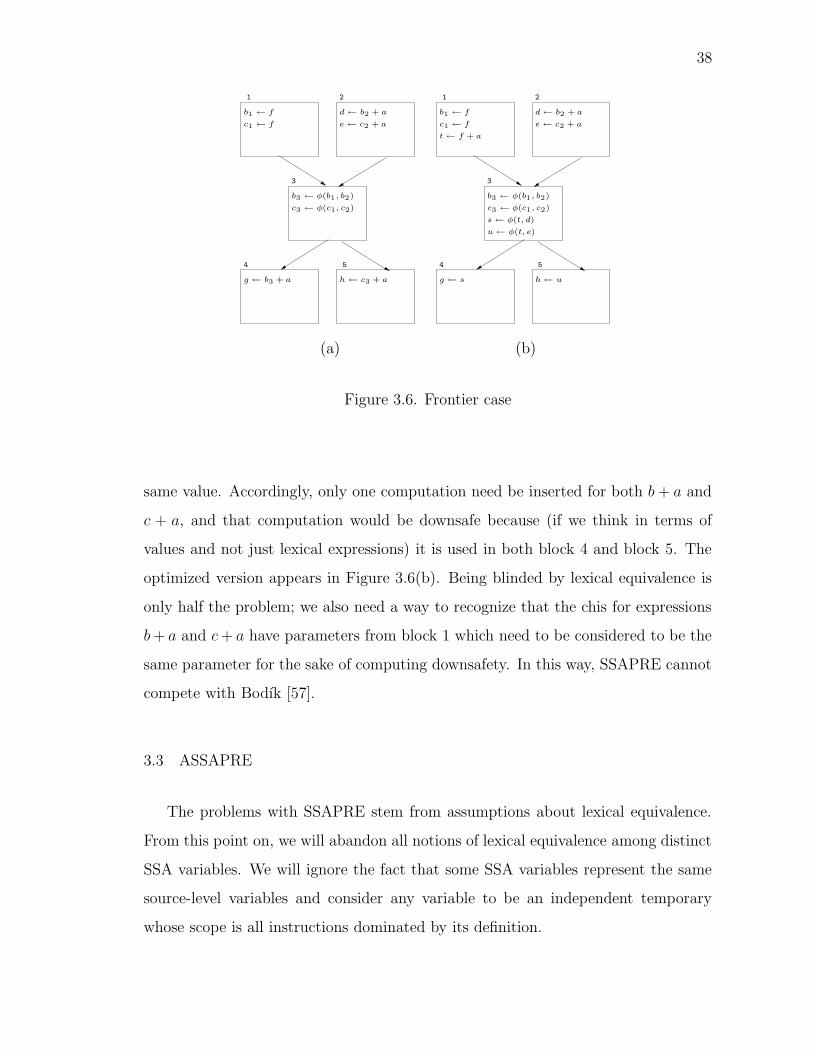
38
b3 ← φ(b1, b2)
d← b2 + a
e← c2 + ac1 ← f
g ← b3 + a
4
3
21
5
b1 ← f
c3 ← φ(c1, c2)
h← c3 + a
b3 ← φ(b1, b2)
d← b2 + a
e← c2 + ac1 ← f
g ← s
4
3
21
5
b1 ← f
c3 ← φ(c1, c2)
h← u
t← f + a
s← φ(t, d)
u← φ(t, e)
(a) (b)
Figure 3.6. Frontier case
same value. Accordingly, only one computation need be inserted for both b+ a and
c + a, and that computation would be downsafe because (if we think in terms of
values and not just lexical expressions) it is used in both block 4 and block 5. The
optimized version appears in Figure 3.6(b). Being blinded by lexical equivalence is
only half the problem; we also need a way to recognize that the chis for expressions
b+ a and c+ a have parameters from block 1 which need to be considered to be the
same parameter for the sake of computing downsafety. In this way, SSAPRE cannot
compete with Bodık [57].
3.3 ASSAPRE
The problems with SSAPRE stem from assumptions about lexical equivalence.
From this point on, we will abandon all notions of lexical equivalence among distinct
SSA variables. We will ignore the fact that some SSA variables represent the same
source-level variables and consider any variable to be an independent temporary
whose scope is all instructions dominated by its definition.

39
As already noted, SSAPRE is characterized by availability: chis are placed at
the dominance frontier of a computation and thus indicate where a value is (at
least partially) available. In this section, we present a new algorithm, Anticipation-
SSAPRE (ASSAPRE) which searches backward from computations and places chis
at merge points where a value is anticipated. If the algorithm discovers the definition
of a variable in the expression for which it is searching, it will alter the form of that
expression appropriately; for example, if it is searching for t3 + t7 and discovers the
instruction t7 ← t1, then from that point on it will look for t3 + t1. (We do not need
also to look for t3 + t7 since t7 is out of scope above its definition.) When a chi is
created, it is allocated a fresh hypothetical temporary, which will be the target of
the phi that will be placed there if the chi is used in a transformation. The result of
this phase is that instructions are assigned temporaries that potentially store earlier
computations of the instructions’ values. The instructions may be replaced by moves
from those temporaries.
Since all variables are distinct, so are all expressions. This obviates the need
for the notion of canonical expressions and the need for version numbers. Thus our
algorithm has no renaming phase. Not only do the problems in SSAPRE come from
ambiguities in the specification of Rename, but also our implementation experience
has found Rename to be particularly prone to bugs [65]. Next, the algorithm analyzes
the chi operands that are ⊥ to determine which ones represent downsafe insertions
and analyzes the chis to determine which ones can be made available, which ones
can be postponed, and, from these, which ones should be made into phis. This
happens in the two phases Downsafety and WillBeAvail. Finally, where appropriate,
insertions are made for chi operands, phis are put in the place of chis, and redundant
computations are replaced with moves from temporaries. This phase, Code Motion,
subsumes the Finalize phase in SSAPRE. Thus, ASSAPRE has four phases from
SSAPRE’s six.
The next subsections describe the four phases of ASSAPRE in detail. We clarify
each step by observing what it does on a running example. The unoptimized version
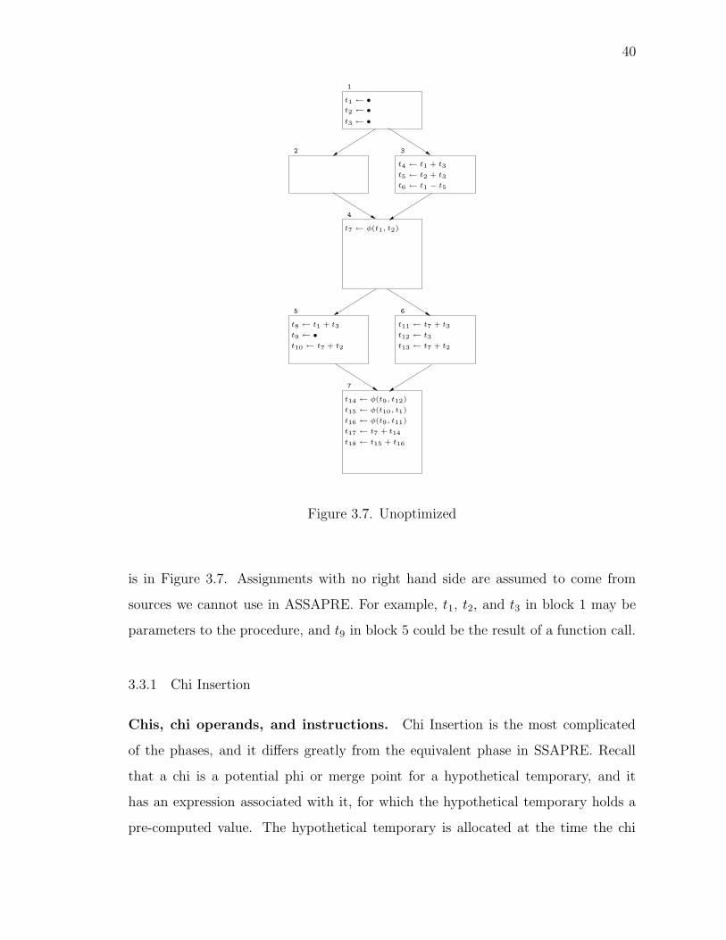
40
t4 ← t1 + t3
t5 ← t2 + t3
t6 ← t1 − t5
4
t7 ← φ(t1, t2)
t10 ← t7 + t2
t9 ← •
t8 ← t1 + t3
t13 ← t7 + t2
t12 ← t3
t11 ← t7 + t3
t14 ← φ(t9, t12)
t15 ← φ(t10, t1)
t16 ← φ(t9, t11)
t17 ← t7 + t14
t18 ← t15 + t16
5 6
7
3
t1 ← •
1
t2 ← •
t3 ← •
2
Figure 3.7. Unoptimized
is in Figure 3.7. Assignments with no right hand side are assumed to come from
sources we cannot use in ASSAPRE. For example, t1, t2, and t3 in block 1 may be
parameters to the procedure, and t9 in block 5 could be the result of a function call.
3.3.1 Chi Insertion
Chis, chi operands, and instructions. Chi Insertion is the most complicated
of the phases, and it differs greatly from the equivalent phase in SSAPRE. Recall
that a chi is a potential phi or merge point for a hypothetical temporary, and it
has an expression associated with it, for which the hypothetical temporary holds a
pre-computed value. The hypothetical temporary is allocated at the time the chi

41
is created, so it is in fact a real temporary from the temporary pool of the IR; it
is hypothetical only in the sense that we do not know at the time it is allocated
whether or not it will be used in the output program. The hypothetical temporary
also provides a convenient way of referring to a chi, since the chi is the hypothetical
definition point of that temporary. In the examples, a chi will be displayed with its
operands in parentheses followed by its hypothetical temporary in parentheses. The
expression it represents is written in the margin to the left of its basic block (see
Figure 3.9).
As before, a chi operand is associated with a CFG edge and either names a
temporary or is ⊥. However, an important feature of our algorithm is that chis at
the same block can share chi operands. Assume that if two chi operands are in the
same block, are associated with the same CFG edge, and refer to the same temporary,
then they are the same. Chi operands that are ⊥ are numbered in our examples to
distinguish them. The temporary to which a chi operand refers is called the definition
of that chi operand, and if the chi operand is ⊥, we say that its definition is null.
Chi operands also have expressions associated with them, as explained below, but
to reduce clutter, they are not shown in the examples.
Real occurrences of an expression (ones that appear in the code and are saved
to a temporary) also have definitions associated with them, just as chi operands do.
This is the nearest temporary (possibly hypothetical) found that contains the value
computed by the instruction. If no such temporary exists, then the definition is ⊥.
In the examples, this temporary is denoted in brackets in the margin to the left of
its instruction. This notion of definition induces a relation among real instructions,
chis, and chi operands and is equivalent to the factored redundancy graph of Chow,
Kennedy et al. [1, 2]
Searching from instructions. Chi Insertion performs a depth-first, preorder
traversal over the basic blocks of the program. In each basic block, it iterates forward
over the instructions. For each instruction on which we wish to perform PRE (in our

42
case, binary arithmetic operations), the algorithm begins a search for a definition.
During the search, it maintains a search expression e, initially the expression com-
puted by the instruction where it starts. It also maintains a reference to the starting
instruction, i. Until it reaches the preamble of the basic block (which we assume
includes the phis and chis), the algorithm inspects an instruction at each step, which
we refer to as the current instruction. Note that the “current instruction” is that
which is current in the inner loop, where as the current instruction in the outer loop
we call the “starting instruction,” i.
The current instruction being inspected is either a computation of e, the definition
point of one of the operands of e, or an instruction orthogonal to e. In practice,
we expect that this last case will cover the majority of the instructions inspected,
and such instructions are simply ignored. If the instruction is a computation of e
(that is, the expression computed exactly matches e), then the search is successful,
and the temporary in which the current expression stores its result is given as the
definition of i. When the current expression defines one of e’s operands, then what
happens depends on the type of instruction. If it is •, then nothing can be done;
the search fails, and i’s definition is null, since a component to e is not live earlier
than this instruction and consequently the search expression cannot exist earlier. If
the current instruction is a move, then we emend the search expression accordingly:
the occurrences in e of the the target of the move are replaced by the move’s source.
The search then continues with the new form of e. Consider the situation in Figure
3.8. The search from instruction t4 ← t1 + t3 begins using t1 + t3 as its search
expression and then hits the instruction t3 ← t2. t1 + t3 certainly cannot exist prior
to that instruction, but the emendation t1 + t2 may. If a copy propagation has been
performed immediately before ASSAPRE, then this should not be necessary, since
moves will be eliminated. However, we make no assumptions about the order in
which optimizations are applied, and in our experience such moves proliferate under
many IR transformations.

43
.
Search Expression
Emended Search Expression
..
..
..
t1 + t2
t1 + t3
t3 ← t2
t4 ← t1 + t3
Figure 3.8. Making an emendation
If the current instruction stores the result of a PRE-candidate computation to an
operand of e, then we make a conjectural emendation of the search expression; that is,
we optimistically assume the instruction will be replaced by a move, and emend e as
if that move were already in place. Since blocks are processed in depth-first preorder
and instructions processed by forward iteration, we know that the instruction being
inspected has already been given a definition. If that definition is not null, then we
can conjecture that the instruction will be replaced by a move from the temporary
of its definition to the temporary being written to, and we emend e as if that move
were already present. From a software engineering standpoint, such conjectural
emendations may be skipped during early development stages. However, they are
necessary for optimality, since they take care of the situation in Figure 3.5. Without
them, ASSAPRE would require multiple runs to achieve optimality, especially in
concert with the enabling optimizations described in Briggs and Cooper [34]. If the
instruction’s definition is null (or if conjectural emendations are turned off), such an
instruction must be treated the same way as •, and the search fails.
When the search reaches the preamble of a block, there are three cases, depending
on how many predecessors the block has: zero (in the case of the entry block), one
(for a non-merge point), or many (for a merge point). At the entry block, the search
fails. At a non-merge point, the search can continue starting at the last instruction
of the predecessor block with no change to i or e (we know that those instructions
already have been given definitions because the predecessor in this case would be
a dominator). Merge points are the interesting case. There the algorithm inspects

44
the expressions represented by the chis already placed in that block. If one is found
to match e, then that chi (or more properly, that chi’s hypothetical temporary) is
given as i’s definition. If no suitable chi is found, the algorithm creates one; a new
temporary is allocated (which becomes i’s definition), and the chi is appended to
the preamble and to a list of chis whose operands need to be processed, as will be
described below. In either case, the search is successful.
Consider the program in Figure 3.7. From the instruction i = t4 ← t1 + t33
in block 3, we search for an occurrence of e = t1 + t3 and immediately hit the
preamble of the block. Since it is not a merge point, the search continues in block
1. The assignment of t3 is relevant to e, but since that instruction is not a move or
a PRE candidate, the search fails and i is assigned ⊥. Similarly, the searches from
t5 ← t2 + t3 and t6 ← t1 − t5 fail. For i = t8 ← t1 + t3, e = t1 + t3, the search
takes us to the preamble of block 4. Since it is a merge point, we place a chi there
with expression t1 + t3 and allocate t19 as its hypothetical temporary, which also
becomes the definition of t8 ← t1 + t3. Similarly for i = t10 ← t7 + t3, we place a chi,
allocating the temporary t20; and for i = t11 ← t7 + t3, a chi with temporary t21. For
i = t13 ← t7 + t2, e = t7 + t2, when the preamble of block 4 is reached, we discover
that a chi whose expression matches e is already present, and so its temporary (t20)
becomes i’s definition. Finally, searches from the two real instructions in block 7
produce the chis with temporaries t22 and t23, which serve as the real instructions’
definitions. Figure 3.9(a) displays the program at this point.
Searching from chi operands. When all basic blocks in the program have been
visited, the algorithm creates chi operands for the chis that have been made. Chi
operands stand in for operands to the phis that may be created later, and since chi
operands have definitions just like real instructions, this involves a search routine
identical to the one above. The only complications are chi-operand sharing among
chis at the same block and emendations with respect to phis and other chis. For each
3Recall that ← denotes assigment in our language; thus = stands for equals in the mathematicaland logical sense.

45
chi c in the list generated by the search routine and for each in-coming edge η at that
block, the algorithm determines an expression for the chi operand for that edge. To
do this, we begin with the chi’s own expression, e, and inspect the phis at the block
and the chis that have already been processed. If any write to an operand of e (that
is, if one of e’s operands is the target of a phi or the hypothetical temporary of a
chi), then that operand must be replaced by the operand of the phi that corresponds
to η or the definition of the chi operand that corresponds to η. (If such a chi operand
is ⊥, then we can stop there, knowing that the chi operand we wish to create will be
⊥, and that it is impossible to make an expression for it.) For example, if e = t4 + t6
and the current block contains t6 ← φ(t1, t2), the left chi operand will have the
expression t4 + t1 and the right will have t4 + t2. We call the revised expression e′.
Once an expression has been determined, the algorithm inspects the chi operands
corresponding to η of all the chis at that block that have already been processed;
if any such chi operand has an expression matching e′, then that chi operand also
becomes an operand of c. This sharing of chi operands is necessary to cross Knoop
et al’s frontier [55] as the examples will show. If no such chi operand is found, the
algorithm creates a new one with e′ as its expression, and it searches for a definition
for it in the same manner as it did for real instructions, in this case i referring to the
chi operand. Note that this may also generate new chis, and the list of chis needing
to be processed may lengthen.
So far, this phase has generated the five chis in Figure 3.9(a). The search for
definitions for their operands is more interesting. In block 4, the t19 chi has expression
e = t1 + t3. Since none of e’s operands are defined by phis, e also serves as the
expression for the chi’s operands. Search from the left operand fails when it hits the
write to t3 in block 1. Search from the right operand, however, discovers t4 ← t1 + t3,
which matches e; so t4 becomes its definition. The t20 chi has expression e = t7 + t2.
Since t7 ← φ(t1, t2) writes to one of e’s operands, the two chi operands will have the
expressions t1 + t2 and t2 + t2. Since neither have occurred in the program, two ⊥ chi
operands are created. The t21 chi has expression e = t7 + t3. The phi changes this to

46
t7 + t2
t1 + t3
t16 ← φ(t9, t11)
χ( , )(t22)
χ( , )(t23)
t17 ← t7 + t14
t18 ← t15 + t16
χ( , )(t21)
χ( , )(t20)
χ( , )(t19)
t15 ← φ(t10, t1)
t14 ← φ(t9, t12)
t11 ← t7 + t3
t12 ← t3
t7 + t3
7
65
[t23]
[t22]
t15 + t16
t7 + t14
[t20]
[t21]
[t20]
[t19]
[⊥]
[⊥]
[⊥]
t13 ← t7 + t2
t8 ← t1 + t3
t9 ← •
t10 ← t7 + t2
t7 ← φ(t1, t2)
4
t6 ← t1 − t5
t5 ← t2 + t3
t4 ← t1 + t3
32
t3 ← •
t2 ← •
1
t1 ← •
[t21]
[t20]
[t19]
[⊥]
[⊥]
[⊥]
t16 ← φ(t9, t11)
χ(⊥4, t11)(t22)
χ(t24, t25)(t23)
t17 ← t7 + t14
t18 ← t15 + t16
χ(⊥1, t5)(t21)
χ(⊥2,⊥3)(t20)
t15 ← φ(t10, t1)
t14 ← φ(t9, t12)
[t20]
t7 + t3
t7 + t2
t1 + t3
t1 − t21
t20 − t19
χ(⊥7, t6)(t25)
χ(⊥5,⊥6)(t24)
χ(⊥1, t4)(t19)
7
65
[t23]
[t22]
t15 + t16
t7 + t14
t11 ← t7 + t3
t1 ← •
t12 ← t3
t13 ← t7 + t2
t8 ← t1 + t3
t9 ← •
t10 ← t7 + t2
t7 ← φ(t1, t2)
4
t6 ← t1 − t5
t5 ← t2 + t3
t4 ← t1 + t3
32
t3 ← •
t2 ← •
1
(a) (b)
Figure 3.9. During Chi Insertion

47
t1 + t3 for the left edge and to t2 + t3 for the right edge. The former is identical to the
expression for the left operand of the t19 chi, so that operand is reused. Searching
from the right chi operand discovers t5 ← t2 + t3.
Turning to block 7, the t22 chi has expression t7 + t14, which the phis change to
t7 + t9 for the left edge and t7 + t12 for the right. On the left side, a search for a
definition for the chi operand halts at t9 ← • in block 5. The right hand search
discovers t11 ← t7 + t3. The left and right chi operands for the t23 chi (e = t15 − t16)
have expressions t10 − t8 and t1 − t11, respectively. On the left, t10 ← t7 + t2 and
t8 ← t1 + t3 in block 5 affect the search expression, which we conjecturally emend
to t20 − t19. When the preamble of block 4 is reached, a new chi must be placed,
allocating the temporary t24. On the right, t11 ← t7 + t3 causes the search expression
to be emended to t1−t21, which also requires a new chi at block 4. Finally, we search
for definitions for the chi operands of the two chis recently placed in block 4. The
program at the end of the Chi Insertion phase is shown in Figure 3.9(b).
Termination. Since the search for a definition for a chi operand may traverse a
back edge, we now convince ourselves that the algorithm will terminate on loops;
indeed, one qualification needs to be made for conjectural emendations in order to
ensure termination. Consider the case when the search from a chi operand brings
us back to the merge point of its chi. If the search expression has not changed, then
the chi itself is the definition, and the search ends; otherwise, if no chi at that merge
matches the current search expression, a new chi will be made. If operands in the
search expression have been replaced only by other temporaries or constants in the
input program (in other words, no conjectural emendations), then this process cannot
go on forever, because there are only a finite number of temporaries or constants in
the code. The danger lies when a temporary has been replaced by a hypothetical
temporary. We say that a chi is complete if searches from all of its chi operands
have been finished, and none refer to chis that are not complete. We say that a chi c
depends on a chi operand ω if ω is an operand of c or if ω is an operand to a chi that

48
......
χ( , t6)(t5)
t3 ← t2 + 1
χ( , t5)(t4)
χ( , )(t6)
[t4]
t2 ← φ(t1, t3)
Figure 3.10. Unterminated Chi Insertion
in turn is referred to by a chi operand on which c depends. Supposing, as above,
that e′ is the search expression when searching for a definition of chi operand ω, then
if the current instruction being inspected writes to an operand of e′ but is defined by
a chi c that does not depend on ω, then this search does not prolong the sequence of
searches that make c complete. If c does depend on ω, we have no such guarantee.
For example, if the expression in question is the increment of a loop counter, the
algorithm would attempt to insert a chi for each iteration—an infinite number. To
see this illustrated, consider Figure 3.10. t1, t2, and t3 represent a loop-counter in
the source code. If we search for an earlier occurrence of t2 +1, we will place a chi for
it at the top of the block. Searching, then, for the chi operands, we emend the search
expression to t3 +1 because of the phi. This leads us back to the original occurrence,
t2 + 1, with target t3. If we were to emend the search expression conjecturally, we
would replace t3 with t4, the occurrence’s definition. Placing a chi, then for t4 + 1,
we search for an operand for the expression t5 + 1, since the previous chi merges t5
into t4. Continuing like this would place chis at this point indefinitely. Thus:
when searching from a chi operand ω, conjectural emendations are for-
bidden if the current instruction is defined by a chi that depends on ω.
The algorithm for this phase is summarize in Figure 3.11.

49
Let ∆ be a mapping from instructions, chis, and chi operands to hypothetical temporariesFor each block b
For each instruction i = t← t′ op t′′
Let e be t′ op t′′, i′ be the instruction preceding i and β be bLoop
If i′ = τ ← γ
If τ appears in eIf γ = τ ′
replace τ in e with τ ′
Else if γ = e and we conjecturally emendreplace τ in e with ∆(i′)
Else if γ = • or we do not conjecturally emend∆(i) := ⊥; break
i′ := the instruction preceding i′
Else if we have reached the preamble of βIf |pred(β)| = 0
∆(i) := ⊥; breakElse if |pred(β)| = 1
β := pred(β)i′ := the last instruction in β
Else if |pred(β)| > 1Find or create a chi c for e with its hypothetical temporary t∗
∆(i) := t∗
Add c to the chi worklist While the chi worklist is not emptyLet c be the next chi on the worklist, e be the expression associated with c,
and b be the block hosting cFor each η ∈ pred(b)
Let e′ be e transformed by the chis and phis at b with respect to ηIf a chi operand ω for e′,η exits
Set that as c’s operand corresponding to ηElse
Create a new ω and search for a definition for using the same loop as above.
Figure 3.11. Algorithm for Chi Insertion

50
We have treated this algorithm as though it were working only on arithmetic
operations (the non-bracketed portion of the language presented in Section 1.2.1).
With a little extension, this algorithm can work on object and array loads as well,
which greatly increases its potency. Care must be taken because objects and arrays
can have aliases that make it difficult to know when two expressions are equivalent,
a problem we explore in depth in Chapter 5. For our present purposes, it is best
to rely on an underlying GVN and alias analysis, as is done in Fink et al’s load
elimination [3] In that case, we search for an instruction (either a load or a store)
that has definitely the same value as the instruction from which we started. The
search fails if we cross a store to something that is not definitely different, since that
could represent a change in the expression’s value. If reads kill [66], then this is true
also for loads that are not definitely different.
3.3.2 Downsafety
Recall that a computation to be inserted is downsafe only if the same computation
is performed on all paths to exit. Avoiding inserting computations that are not
downsafe prevents lengthening computation paths and causing exceptions that would
not be thrown in the unoptimized program. Since chi operands represent potential
insertions, we consider downsafety to be a property of chi operands rather than of chis
as in Chow, Kennedy, et al [1,2] and Table 3.2. The second phase of ASSAPRE is a
static analysis that determines which chi operands are downsafe. We are interested
only in chi operands that are ⊥ or defined by a chi, because these are potential
insertion points: if a chi operand’s definition is the result of a real instruction, no
insertion would ever need to be made for it, but a ⊥ chi operand would certainly
need an insertion; a chi operand defined by another chi would need an insertion if
no phi is made for its defining chi. The question of whether a chi operand’s value is
used on all paths to program exit is akin to liveness analysis for variables and can be
determined by a fixed-point iteration. At the entry to a block that is a merge-point,

51
the chi operands of the chis there become “live.” A use of their value—which happens
if a real instruction has the hypothetical temporary of the chi as a definition—“kills”
them. All chi operands that are not killed in that block are “live out,” and must be
considered “live in” for the block’s successors.
The fact that chis share chi operands complicates downsafety, since if a chi
operand is an operand to several chis, a use of any of their hypothetical tempo-
raries will kill it. Moreover, the use of a chi’s hypothetical temporary will kill all of
that chi’s chi operands. To handle this, in addition to a set of live chi operands, we
must maintain on entry and exit of every block a mapping from temporaries to sets
of chi operands which a use of the temporaries will kill.
What if a killing temporary for a chi operand is used as the definition to another
chi operand? We could consider that chi operand to be a use occurring at the end
of the corresponding predecessor block (not in the block that contains its chi). That
would complicate things because if the chi operand was the only killer for the first
chi operand on a path to exit, then the downsafety of the first would depend on the
downsafety of the second. SSAPRE handled this by propagating a false value for
downsafety from chis already found to be false to chis that depended on them. We
can handle this with our map structure: if a use of t1 will kill chi operand ω1, chi
operand ω2 has t1 as its definition, and a use of t2 will kill ω2, then we say that t2
will also kill ω1. The effect this has is that the use of a temporary as the definition
of a chi operand cannot itself kill another chi operand, but that the fate of both chi
operands are linked on subsequent paths to exit. One thing should be noted, though:
if a chi appears at the beginning of a loop and is the definition of another chi there,
its operand will have the temporaries of both chis as killers. If the second chi turns
out not to be inserted but is the definition of a real occurrence in the block, a chi
operand in the first chi may be wrongly killed and the chi wrongly thought downsafe.
To correct this, when a chi operand is new at the beginning of a basic block, only
the chis that have it as an operand should define a kill for it.

52
live in(b) = (⋃
p∈pred(b) live out(p))⋃
chi operands at b
map in(b) = clear b(⋃
p∈pred(b) map out(p))⋃
t 7→ σ | chi at b with temporary tand set of chi operands σ
live out(b) = live in(b)−ω | ∆(i) = t and map in(t) = ω
for some instruction i ∈ bor for some correspondingchi operand i in a successor
map out(b) = map in(b)clear b(m) = t 7→ σ | t 7→ σ′ ∈ m and σ = σ′ −Ω
where Ω is the set of chi operands at b
Figure 3.12. Data flow equations for Downsafety
Suppose live in(b), live out(b), map in(b), and map out(b) are the live in and
out sets and mappings in and out, respectively, for a block b, and that ∆(i) finds
the definition of instruction i. Then to compute downsafety, we must solve the data
flow equations in Figure 3.12.
Table 3.3 lists what chi operands are downsafe in our example and explains why.
As in the Figures, chi operands are identified by their definition or ⊥. Of particular
interest is ⊥1 because it is downsafe only because it is shared—it is killed on the left
path because it belongs to the t19 chi and on the right because it belongs to the t21
chi. If these were considered separate chi operands, then an opportunity to eliminate
a redundancy would be missed.
Extra care needs to be taken when optimizing a program in a language that
supports precise handling of exceptions, such as Java. Instructions that could throw
an exception (like any division where the denominator could be zero) must not be
reordered, which could happen by the insertions and eliminations done by this algo-
rithm. We solve this elegantly with a slight modification to the Downsafety phase.
If we are checking the downsafety of a chi operand that represents an expression
that could except, a use that occurs after another potentially excepting instruction

53
Table 3.3Downsafety for the running example
⊥1 downsafe: killed by t8 ← t1 + t3 on the left path and t11 ← t7 + t3 onthe right.
t4 Irrelevant: defined by real instruction.⊥2 downsafe: killed by t10 ← t7 + t2 on the left path and t13 ← t7 + t2 on
the right.⊥3 downsafe: killed by t10 ← t7 + t2 on the left path and t13 ← t7 + t2 on
the right.t5 Irrelevant: defined by real instruction.⊥5 Not downsafe.⊥6 Not downsafe.⊥7 Not downsafe.t6 Irrelevant: defined by real instruction.⊥4 downsafe: killed by t17 ← t7 + t14.t11 Irrelevant: defined by real instruction.t24 downsafe: killed by t18 ← t15 + t16.t25 downsafe: killed by t18 ← t15 + t16.
should not make the chi operand considered downsafe. So when a potentially ex-
cepting instruction is encountered during Downsafety, all potentially excepting chi
operands should be killed.
3.3.3 WillBeAvail
The WillBeAvail stage computes the remaining properties for chis and chi operands,
namely, canBeAvail, later, and willBeAvail for chis and insert for chi operands, as
listed in Table 3.5. The most important of these is willBeAvail because it character-
izes chis that will be turned into phis for the optimized version.
We first determine whether it is feasible and safe for a chi to be made into a
phi. If all of a chi’s operands either have a real use or are downsafe, then that chi is
canBeAvail. A chi is also canBeAvail if all of its chi operands that are not downsafe
are defined by chis which also are canBeAvail, since, even though an insertion for that
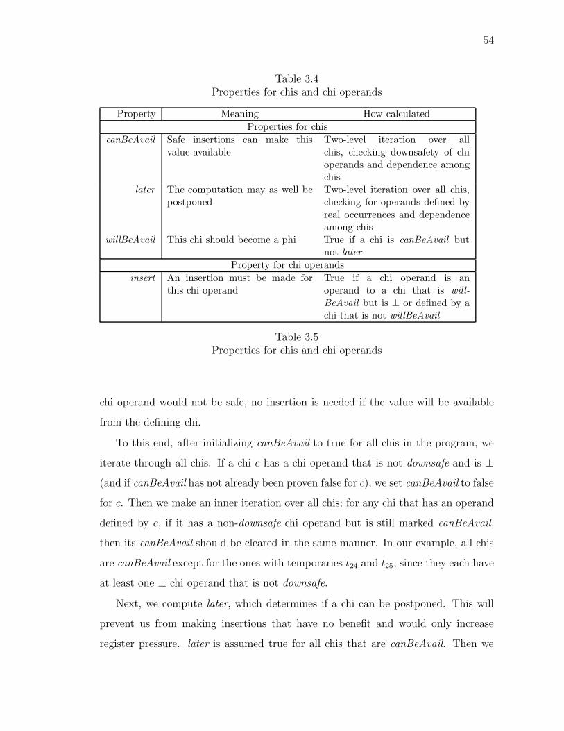
54
Table 3.4Properties for chis and chi operands
Property Meaning How calculated
Properties for chis
canBeAvail Safe insertions can make thisvalue available
Two-level iteration over allchis, checking downsafety of chioperands and dependence amongchis
later The computation may as well bepostponed
Two-level iteration over all chis,checking for operands defined byreal occurrences and dependenceamong chis
willBeAvail This chi should become a phi True if a chi is canBeAvail butnot later
Property for chi operands
insert An insertion must be made forthis chi operand
True if a chi operand is anoperand to a chi that is will-
BeAvail but is ⊥ or defined by achi that is not willBeAvail
Table 3.5Properties for chis and chi operands
chi operand would not be safe, no insertion is needed if the value will be available
from the defining chi.
To this end, after initializing canBeAvail to true for all chis in the program, we
iterate through all chis. If a chi c has a chi operand that is not downsafe and is ⊥
(and if canBeAvail has not already been proven false for c), we set canBeAvail to false
for c. Then we make an inner iteration over all chis; for any chi that has an operand
defined by c, if it has a non-downsafe chi operand but is still marked canBeAvail,
then its canBeAvail should be cleared in the same manner. In our example, all chis
are canBeAvail except for the ones with temporaries t24 and t25, since they each have
at least one ⊥ chi operand that is not downsafe.
Next, we compute later, which determines if a chi can be postponed. This will
prevent us from making insertions that have no benefit and would only increase
register pressure. later is assumed true for all chis that are canBeAvail. Then we

55
iterate through all chis, and if a chi c is found for which later has not been proved false
and which has an operand defined by a real occurrence, we reset later for it. To do
this, we not only set later to false, but, similarly to how canBeAvail was propagated,
we also iterate through all chis; if any is found that has an operand with c as a
definition, that chi’s later is reset recursively. The idea is that if the definitions of
any of a chi’s variables are available (either because they are real occurrences or
because they are chis that cannot be postponed), the chi itself cannot be postponed.
In our example (see Figure 3.9) the t20 chi is later because both of its operands are
⊥. The t23 chi is also later because both of its operands come from chis for which
canBeAvail is false. These computations can be postponed.
At this point, computing willBeAvail is straightforward. A chi will be available
if it can be made available and there is no reason for it not to be—that is, if it is
canBeAvail and not later. In our example, all chis are willBeAvail except for the
ones associated with t20, t24, and t25. This property can be computed on demand
based on stored values for willBeAvail and later. From this we also can compute
insert, which characterizes chi operands that require a computation to be inserted.
A chi operand is insert if it belongs to a willBeAvail chi and is either ⊥ or defined by
a chi for which willBeAvail is false. Being in a willBeAvail chi implies that such a chi
operand is downsafe. In our example, chi operands ⊥1 and ⊥4 are insert. willBeAvail
and insert can be computed on demand when they are needed in the next phase.
3.3.4 CodeMotion
The earlier phases having gathered information, the final stage, CodeMotion,
transforms the code by inserting phis and anticipated computations and eliminating
redundant computations. The net effect is to hoist code to earlier program points.
If willBeAvail is true for a chi, then the value it represents should be available in a
temporary in the optimized program; a phi needs to be put in its place to merge the
values on the incoming paths. The operands to this new phi will be the temporaries

56
that hold the values from the various predecessors. If insert is true for any of its
operands (indicating that the value it represents is not available, that is, has not
been computed and stored in a temporary), then a computation for that value must
be inserted at the end of the predecessor block it represents. Any real occurrence
whose definition is another real occurrence or a willBeAvail chi is redundant, and
can be replaced with a move from the temporary holding its value—if it is defined
by a chi, the temporary is the target of the phi put in place of the chi; if it is defined
by a real occurrence, the temporary is the one for the result of that occurrence.
Three steps complete the changes to the code: Inserting appropriate computa-
tions, creating new phis, and eliminating fully redundant computations.
To do the insertions, we iterate over all chi operands. If any is marked insert,
then we allocate a new temporary, manufacture an instruction which computes the
chi operand’s expression and stores the result in the fresh temporary, append that
instruction at the end of the corresponding basic block, and set the fresh temporary to
be the chi operand’s definition. In our example, ⊥1 requires us to insert t26 ← t1 + t3
in block 2, where t26 is fresh. Similarly, we insert t28 ← t7 + t9 at block 5 for ⊥4.
We then iterate over all chis. For a chi c that willBeAvail, we insert a phi at the
end of the list of phis already present at the block. That phi merges the temporaries
that define c’s chi operands into c’s hypothetical temporary. Because insertions
have been made, all valid chi operands will have temporaries for definitions by this
point. In our example, we create t19 ← φ(t26, t4) and t21 ← φ(t26, t5) in block 4 and
t22 ← φ(t28, t11) in block 7.
Finally, we iterate over all instructions. If any is defined by the target of another
real instruction or of a willBeAvail chi (which by this time has been made into a
phi), it is replaced with a move instruction from its definition to its target. In our
example, t11 ← t7 + t3 in block 6 is replaced with t11 ← t21, and t17 ← t7 + t14 in
block 7 is replaced with t17 ← t22.
An algorithmic description is found in Figure 3.13.
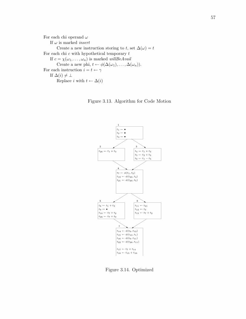
57
For each chi operand ωIf ω is marked insert
Create a new instruction storing to t, set ∆(ω) = t
For each chi c with hypothetical temporary tIf c = χ(ω1, . . . , ωn) is marked willBeAvail
Create a new phi, t← φ(∆(ω1), . . . ,∆(ωn)).For each instruction i = t← γ
If ∆(i) 6= ⊥Replace i with t← ∆(i)
Figure 3.13. Algorithm for Code Motion
t6 ← t1 − t5
4
t7 ← φ(t1, t2)
t10 ← t7 + t2
t9 ← •
t8 ← t1 + t3
t13 ← t7 + t2
t12 ← t3
t11 ← t21
t14 ← φ(t9, t12)
t15 ← φ(t10, t1)
t18 ← t15 + t16
t17 ← t7 + t14
t22 ← φ(t28, t11)
t16 ← φ(t9, t11)
5 6
7
t19 ← φ(t26, t4)
t21 ← φ(t26, t5)
t26 ← t1 + t3
t28 ← t7 + t9
t5 ← t2 + t3
t1 ← •
1
t2 ← •
t3 ← •
2 3
t4 ← t1 + t3
Figure 3.14. Optimized
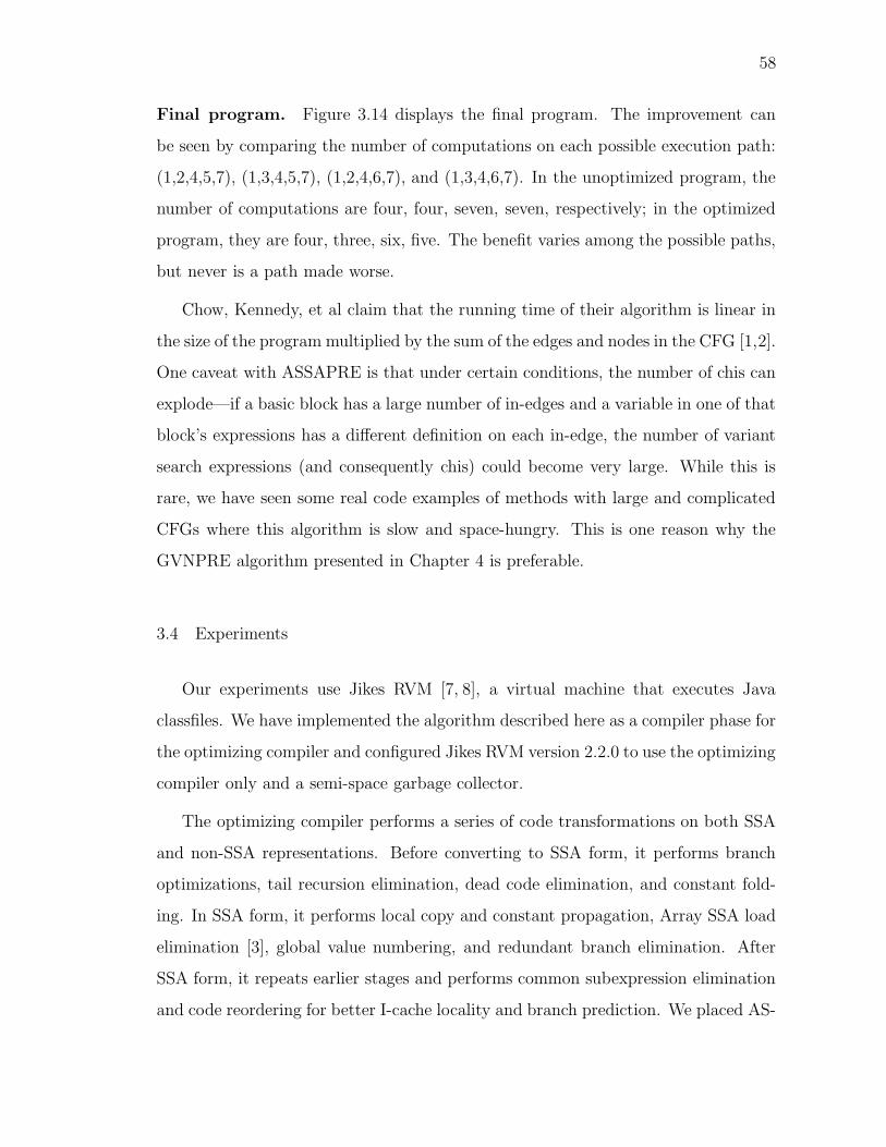
58
Final program. Figure 3.14 displays the final program. The improvement can
be seen by comparing the number of computations on each possible execution path:
(1,2,4,5,7), (1,3,4,5,7), (1,2,4,6,7), and (1,3,4,6,7). In the unoptimized program, the
number of computations are four, four, seven, seven, respectively; in the optimized
program, they are four, three, six, five. The benefit varies among the possible paths,
but never is a path made worse.
Chow, Kennedy, et al claim that the running time of their algorithm is linear in
the size of the program multiplied by the sum of the edges and nodes in the CFG [1,2].
One caveat with ASSAPRE is that under certain conditions, the number of chis can
explode—if a basic block has a large number of in-edges and a variable in one of that
block’s expressions has a different definition on each in-edge, the number of variant
search expressions (and consequently chis) could become very large. While this is
rare, we have seen some real code examples of methods with large and complicated
CFGs where this algorithm is slow and space-hungry. This is one reason why the
GVNPRE algorithm presented in Chapter 4 is preferable.
3.4 Experiments
Our experiments use Jikes RVM [7, 8], a virtual machine that executes Java
classfiles. We have implemented the algorithm described here as a compiler phase for
the optimizing compiler and configured Jikes RVM version 2.2.0 to use the optimizing
compiler only and a semi-space garbage collector.
The optimizing compiler performs a series of code transformations on both SSA
and non-SSA representations. Before converting to SSA form, it performs branch
optimizations, tail recursion elimination, dead code elimination, and constant fold-
ing. In SSA form, it performs local copy and constant propagation, Array SSA load
elimination [3], global value numbering, and redundant branch elimination. After
SSA form, it repeats earlier stages and performs common subexpression elimination
and code reordering for better I-cache locality and branch prediction. We placed AS-
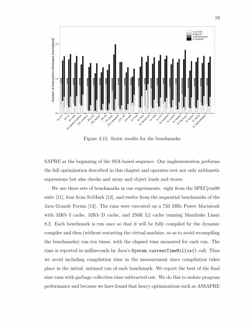
59
Sci−FFT
Sci−LU
Sci−SOR
Sci−Spa
rseC
ompR
ow
_201
_com
pres
s
_202
_jess
_205
_ray
trace
_209
_db
_213
_java
c
_222
_mpe
gaud
io
_227
_mtrt
_228
_jack
Gr−Cry
pt
Gr−Eule
r
Gr−M
onte
Carlo
Gr−SOR
Gr−FFT
Gr−Hea
pSor
t
Gr−LU
Fact
Gr−M
olDyn
Gr−Ray
Trace
r
Gr−Sea
rch
Gr−Ser
ies
Gr−Spa
rseM
atM
ult0.0
1.0
2.0
Num
ber
of in
stru
ctio
ns e
limin
ated
(no
rmal
ized
)
Local CSEGlobal CPLoad EliminationA−SSAPRE
Figure 3.15. Static results for the benchmarks
SAPRE at the beginning of the SSA-based sequence. Our implementation performs
the full optimization described in this chapter and operates over not only arithmetic
expressions but also checks and array and object loads and stores.
We use three sets of benchmarks in our experiments: eight from the SPECjvm98
suite [11], four from SciMark [12], and twelve from the sequential benchmarks of the
Java Grande Forum [13]. The runs were executed on a 733 MHz Power Macintosh
with 32Kb I cache, 32Kb D cache, and 256K L2 cache running Mandrake Linux
8.2. Each benchmark is run once so that it will be fully compiled by the dynamic
compiler and then (without restarting the virtual machine, so as to avoid recompiling
the benchmarks) run ten times, with the elapsed time measured for each run. The
time is reported in milliseconds by Java’s System.currentTimeMillis() call. Thus
we avoid including compilation time in the measurement since compilation takes
place in the initial, untimed run of each benchmark. We report the best of the final
nine runs with garbage collection time subtracted out. We do this to isolate program
performance and because we have found that heavy optimizations such as ASSAPRE

60
left the heap in such a state that later garbage collection times were greater during
the run of the program than if the optimizations had not been performed.
Since ASSAPRE is an expensive optimization, we study its effects on Jikes RVM
optimization level O2. We were particularly interested in how it competes against
other optimizations that do code motion or eliminate computations. Accordingly,
the four optimization phases we are concerned with are local common subexpression
elimination (Local CSE), global code placement (Global CP, which includes global
common subexpression elimination and loop invariant code motion), load elimination
(Load Elimination), and the optimization presented here (ASSAPRE). Given these
optimization phases, we define the following three optimization levels:
O2: To mark our competition, we run the benchmarks at the pre-defined O2 level,
which includes Local CSE, Global CP, and Load Elimination, but not ASSAPRE.
PRE: To measure the effect of ASSAPRE directly, we run ASSAPRE without the
other phases listed except for Local CSE (to clean up a few superfluous checks
generated by our hoisting potentially excepting exceptions).
BOTH: To observe synergies, we run all four phases.
Figure 3.15 presents the static results of the optimization by giving the number
of instructions eliminated by each optimization at each level. The bars for each
benchmark from left to right represent the number of instructions eliminated at
O2, PRE, and BOTH, respectively. The numbers are normalized so that the total
number of instructions eliminated at O2 sum to 1. These results should be used only
to give a feel for how much motion is being done, since this ignores the fact that
at the same time instructions are also being inserted for hoisting. Therefore each
eliminated instruction, at least in the case of ASSAPRE, should be considered as at
least one execution path being shortened by one instruction. We see that ASSAPRE
can eliminate a larger number of instructions than Global CP and Load Elimination
and subsumes much of what they do. In most cases, the number of instructions Load

61
Sci−FFT
Sci−LU
Sci−SOR
Sci−Spa
rseC
ompR
ow
_201
_com
pres
s
_202
_jess
_205
_ray
trace
_209
_db
_213
_java
c
_222
_mpe
gaud
io
_227
_mtrt
_228
_jack
Gr−Cry
pt
Gr−Eule
r
Gr−M
onte
Carlo
Gr−SOR
Gr−FFT
Gr−Hea
pSor
t
Gr−LU
Fact
Gr−M
olDyn
Gr−Ray
Trace
r
Gr−Sea
rch
Gr−Ser
ies
Gr−Spa
rseM
atM
ult
Geom
etric
mea
n0.0
1.0
2.0
O2PREBOTH
Figure 3.16. Speedup on benchmarks
Elimination eliminates at the BOTH level is negligible. However, Load Elimination
and Global CP were not completely subsumed. One reason for this, we found, was
that in some cases (particularly for loop invariant code motion) an instruction was
being moved earlier or later in the loop without any redundant computation being
eliminated or that loop invariant code motion was doing speculative motion that was
not downsafe. The optimizations also had different constraints on what methods they
could be applied to—since the optimizing compiler inlines very aggressively, some
methods became too large to apply these optimizations practically, and there were
some methods Global CP could run on that ASSAPRE could not and vice versa.
We also considered how these transformations impact performance. Figure 3.16
shows speedups for the three optimization levels over a fourth level: O2 with all four
optimizations turned off. Removing redundant instructions does not always signifi-
cantly impact performance. However, on certain benchmarks we achieved speedups
of up to 1.6. ASSAPRE does about as well as global code placement and load elim-
ination combined, and in many cases slices off a little more execution time. On

62
two benchmarks (SciMark’s SparseCompRow and Grande’s MolDyn), it performs
significantly better than its rivals.
In summary, we have demonstrated that ASSAPRE is a complete PRE algorithm
which competes with common subexpression elimination, loop invariant code motion,
and load elimination, both statically and dynamically.
3.5 Conclusion
The contribution of this chapter is a simpler version of SSAPRE that makes
fewer assumptions and covers more cases. The error-prone Rename phase has been
eliminated, Downsafety has been recast as a version of a standard data flow problem,
the algorithm no longer makes assumptions about the namespace, and a wider range
of redundancies are eliminated. It is now fit to be used in conjunction with other
optimizations. Perhaps the best contribution of this algorithm is didactic and experi-
ential: by removing the dependence of SSAPRE on source-level lexical equivalence,
we have moved it one step closer to GVN. The experience with an anticipation-
oriented algorithm prepares us for applying anticipation to GVN as we cross-breed
it with PRE in the next chapter.

63
4 VALUE-BASED PARTIAL REDUNDANCY ELIMINATION
. . . and then [Men] would or could be made to mate with Orcs, producing new breeds,often larger and more cunning. There is no doubt that long afterwards, in the ThirdAge, Saruman rediscovered this, or learned of it in lore, and in his lust for masterycommitted this, his wickedest deed: the interbreeding of Orcs and Men, producing bothMen-orcs large and cunning, and Orc-men treacherous and vile.
—J.R.R. Tolkien, Morgoth’s Ring
4.1 Introduction
Recall that in Muchnick’s view of value numbering (based on the ARWZ strain
of GVN), neither GVN nor PRE is strictly more powerful than the other [47], as
illustrated in Figure 2.1. In Chapter 2, we posed the question, can lexical PRE
be extended to consider a value-based view. In other words, can ARWZ GVN be
extended to consider partial redundancies. In yet other words, can there be an
algorithm that is a complete hybrid of PRE and GVN, subsuming both? Answering
this challenge, we have found a technique, GVNPRE, that does subsume both and
eliminates redundancies that would be undetected by either working in isolation. We
create a system of data flow equations that, using the infrastructure of a simple hash-
based value numbering system, calculates insertion points for partially redundant
values rather than partially redundant expressions. We present this in a framework
that allows clear reasoning about expressions and values and implement it with an
algorithm that can easily be reproduced. Our implementation subsumes GVN.
4.1.1 Overview
In this chapter, we present a new algorithm for PRE on values which subsumes
both traditional PRE and GVN. Section 4.2 gives preliminaries, such as assumptions
we make about the input program, precise definitions of concepts we use for our
analysis, and descriptions of global value numbering infrastructure we assume already

64
available. Section 4.3 contains the meat of the chapter, describing the various phases
of the approach both formally and algorithmically. We comment on several corner
cases in Section 4.4. The algorithm is discussed in the context of other research in
Section 4.5. Section 4.6 gives details on our implementation and its results. We
conclude by discussing its advantages and shortcomings in Section 4.7.
4.2 Framework
In this section, we present our framework in terms of the model of expressions
and values we use. Recall the assumptions about program structure from Section
1.2; this chapter uses the non-bracketed portion of the language.
4.2.1 Values and expressions
A value is a set of expressions grouped together by static analysis of their compu-
tational result. v ranges over values. An expression is similar to an operation except
that if an expression involves an operator, its operands are given in terms of values.
This way we can think of expressions more generally. If t1 and t3 are members of
value v1, and t2 is a member of v2, we need not think of t1 + t2 and t3 + t2 as separate
expressions; instead, we think only of the expression v1 + v2.
e ::= t | v op v Expressions
4.2.2 The value table
Our goal in value numbering is to obtain three pieces of information: value num-
bers, available expressions, and anticipated expressions. Traditional ARWZ GVN
requires only the first two. First, we partition all expressions in the program into
values. We represent this partition with a map (or value table), ∆, with the following
operations in Figure 4.1.

65
add(∆, e, v) ≡ Set v to be e’s value in ∆; add e to the set v.
lookup(∆, e) ≡ Return e’s value, null if none has been set.(For smarter value numbering, assume thisfunction recognizes algebraic identities.)
lookup or add(∆, e) ≡ Do the following:
x := lookup(∆, e)if (x = null)v := x := add(e, v)
return x
Figure 4.1. Operations for the value table
We treat the value table as a black box, but assume it to be used for a simple
hashing value number scheme (such as Click’s [43]), recognizing expressions by their
structure and, if smart enough, algebraic properties, associating them with values.
It is worth noting that any notion of completeness depends on the smarts of the the
function lookup. Two expressions are in the same value if lookup recognizes them to
have the same value, and this is more of an engineering question than a theoretical
one because there is no limit on how smart the function lookup is engineered to be.
For example, if v1 contains 1, v2 contains 2, v4 contains v3 + v1 for some v3, and v5
contains v4 + v1, then v5 also should contain v3 + v2. To enumerate all such cases
would be infinite.1
Figure 4.2(a) displays a running example we will refer to throughout this and
the next section. Since it is large, we will often discuss only part of it at a time.
For the present, consider block 4. The table in Figure 4.2(b) displays the values
referenced in the block and the expressions they contain. For clarity, we assign a
value the same subscript as one of its temporaries wherever possible. Values v1, v2,
and v3 are defined in blocks that dominate block 4, so they are in scope here. The
1The author thanks Di Ma for this insight.

66
2
3
4 5
6
t3 ← t2 + 1
t4 ← t2 + t3
t5 ← t4
t6 ← t1 + t5
t7 ← t3 + 1
t8 ← φ(t1, t7)
t13 ← t12 + t3
t9 ← t2 + t3
t10 ← t9 + t8
t11 ← •
t12 ← t9 + t11
1
t1 ← •
t2 ← φ(t1, t3)
values
v1: t1v2: t2v3: t3v4: t4, v2 + v3, t5v6: t6, v1 + v4
temps generated:
t4, t5, t6exprs generated:
t2, t3, t4, t1, t5, v2 + v3, v1 + v4
(a) Program CFG (b) Values, temporaries, andexpressions of block 4
v11 : t11
v3 : t3v2 : t2
v8 : t8
v10 : v4 + v8
v4 : v2 + v3
v12 : v4 + v11
v13 : v12 + v3
v4 : v2 + v3
v10 : v4 + v8
v8 : t8
v2 : t2 v3 : t3
(c) Anticipated expressions at block 6, (d) Actual anticipated expressionsnot considering the kill of t11 at block 6
Figure 4.2. Running example

67
instruction t4 ← t2 + t3 leads us to discover expressions v2 + v3 and t4 as elements
of the same value, which we call v4. Because of the move t5 ← t4, t5 is also in v4.
Finally, v1 + v5 and t6 are in a value we call v6. Recall that these values are global,
so we are showing only part of the value table for the entire program (in fact, values
v3 and v4 have more members, discovered in other parts of the program).
4.2.3 The available sets
The second piece of information is what expressions are available to represent
the values; or, put differently, what values are already computed and stored in tem-
poraries at a given program point. If more than one temporary of the same value
is live at a point, we want to pick one as the leader [51], which will be used as
the source of the value to replace an operation of that value with a move. To be
unambiguous, we postulate the leader to be the “earliest” temporary available; that
is, the temporary whose defining instruction dominates the defining instructions of
all other temporaries of that value live at that point. We define the leader set to
be the set of leaders representing available values at a program point, where “pro-
gram points” occur before and after each instruction. Although by our theoretical
definition, there is a leader set for any program point, we abstract the notion by
looking at only the sets at the end of a basic block, AVAIL OUT. We shall see that
these are the only ones needed for our algorithm. The leaders available out of block
4 are those expressions listed first for each value in Figure 4.2(b). (This notion of
availability is sometimes called upsafety [55].)
4.2.4 The anticipated sets
Finally, we want to know what values are anticipated at a program point; that
is, will be computed or used on all paths from that point to program exit. Just
as we want appropriate temporaries to represent values in the leader set, so we
want appropriate expressions to represent anticipated values—that is, anticipated

68
values should also have a reverse-flow leader or antileader. An antileader can be a
live temporary or a non-simple expression whose operands are represented in the
antileader set. This is so that the expression could become available by an insertion
at that point, or several insertions if it is a nested expression. Conversely from the
leader set, we are interested only in the antileader sets at the beginning of basic
blocks, ANTIC IN.
Although our method for computing antileader sets presented later is much dif-
ferent, it may be more easily understood initially if we compare this to parts of the
algorithm for ASSAPRE. Suppose we iterated backwards over the instructions in
a basic block as in Chi Insertion 3.3.1, but instead of searching for a specific ex-
pression, we collect the expressions (including the temporaries that stand for their
subexpressions) which we find as a set which will become the antileader set of the
block. For an antileader set, it does not matter which expression represents a value,
so long as that value is live. A temporary potentially in ANTIC IN becomes dead if
it is written to. This is a consequence of SSA form and is similar to what happens
when ASSAPRE crosses the definition of a temporary in the search expression. If
the assignment is from something for which we can make an expression (as opposed
to •), that expression replaces the temporary as the antileader. If the assignment is
from •, then the value is no longer represented at all (consider that if a temporary is
defined by a •, then nothing else can be in the same value). Furthermore, any other
expression that has that (no longer represented) value as an operand also becomes
dead. Therefore antileaders and the values they represent are killed by definitions
of temporaries in the block. An antileader set can be pictured as a dag. Consider
basic block 6 in Figure 4.2(a), alternately with and without the instruction t4 ← •.
In the case where we exclude that instruction, assume t4 to be global. Without
the definition of t4, ANTIC IN can be represented by the dag in Figure 4.2(c). The
nodes of the dag are pairs of values and the antileaders representing them; edges
are determined by the operands of the antileader. If we suppose the block contains

69
t6 ← • as it does in the program, then v4 : t4 is killed, along with all expressions
that depend on v4 also, in cascading effect. See Figure 4.2(d).
Other sets. To calculate these sets, we find two other pieces of information useful:
the temporaries generated by a block, meaning those that are defined; and the
expressions generated by a block, meaning those that occur as operations, operands
to operations, or sources of moves. We say that the block “generates” these because
they will be used as “gen” sets for the flow equations we define in the next section
for computing the leader and antileader sets. These are given for block 4 in Figure
4.2(b).
4.3 GVNPRE
The GVNPRE algorithm has three steps: BuildSets, Insert, and Eliminate.
BuildSets, which we describe formally and algorithmically, populates the value table
and the leader and antileader sets. Insert places new instructions in the program to
make partially available instructions fully available. Eliminate removes computations
whose values are already available in temporaries or as constants.
4.3.1 BuildSets
Flow equations. To compute AVAIL IN and AVAIL OUT for a block, we must con-
sider not only the contents of the block itself, but also expressions inherited from
predecessors (for AVAIL OUT) and anti-inherited from successors (for ANTIC IN).
For this we use a system of flow equations. As is common for flow equations, we also
define the sets AVAIL IN and ANTIC OUT, although only AVAIL OUT and ANTIC IN
are used later in the optimization. We have three gen sets, EXP GEN(b) for ex-
pressions (temporaries and non-simple) that appear in the right hand side of an
instruction in b; PHI GEN(b) for temporaries that are defined by a phi in b; and
TMP GEN(b) for temporaries that are defined by non-phi instructions in b. There

70
are no kill sets for calculating AVAIL OUT, since SSA form implies no temporary is
ever killed. For ANTIC IN, TMP GEN acts as a kill set. Since an available expression
must be defined in an instruction that dominates the program point in question, so
in calculating AVAIL OUT, we consider inherited expressions only from the block’s
dominator. In terms of flow equations,
AVAIL IN[b] = AVAIL OUT[dom(b)] (4.1)
AVAIL OUT[b] = canon(AVAIL IN[b] ∪ PHI GEN(b) (4.2)
∪TMP GEN(b))
where canon is a procedure that, given a set of temporaries, partitions that set into
subsets which all have the same value and chooses a leader from each. Of course
canon would be inconvenient and inefficient to implement; instead, AVAIL OUT[b]
can be calculated easily and efficiently at the same time as the gen sets, as we will
show later.
For ANTIC IN, handling successors is more complicated. If there is only one
successor, we add all its antileaders to AVAIL OUT of the current block; however, we
must translate some temporaries based on the phis at the successor. For example,
if t1 is anticipated by block b, and block b has a phi which defines t1 and has t2
as an operand from block c, then t2, rather than t1, is anticipated at the end of
block c, and it has a different value. For this we assume a function phi translate
which takes a successor block, a predecessor block (i.e., there is an edge from the
second block to the first), and a temporary; if the temporary is defined by a phi at
the successor, it returns the operand to that phi corresponding to the predecessor,
otherwise returning the temporary. If there are multiple successors, then there can
be no phis (because of critical edge removal), but only values anticipated by all of the
successors can be anticipated by the current block. This assures that all anticipated
expressions are downsafe—they can be inserted with confidence that they will be
used on all paths to program exit.

71
v? : v4 + v7
v10 : v4 + v8
t9 ← t2 + t3
t10 ← t9 + t8
t11 ← •
t13 ← t12 + t3
t8 ← φ(t1, t7)
t7 ← t3 + 1
6
5
Figure 4.3. Translation through phis
The flow equations for calculating the antileader sets are
ANTIC OUT[b] =
e|e ∈ ANTIC IN[succ0(b)]∧
∀ b′ ∈ succ(b), ∃e′ ∈ ANTIC IN[b′]|
lookup(e) = lookup(e′) if |succ(b)| > 1
phi translate(ANTIC IN[succ(b)], b,
succ(b)) if |succ(b)| = 1
(4.3)
ANTIC IN[b] = clean(canonEXP(ANTIC OUT[b] ∪ EXP GEN[b] (4.4)
−TMP GEN[b]))
When phi translate translates expressions through phis, it may involve creating
expressions that have not been assigned values yet and therefore require new values
to be created. Consider calculating ANTIC OUT[B5] in our example. Value v10 is
represented by v4 + v8, which is translated through the phi to v4 + v7. However,
that expression does not exist in the program—it needs a new value. See Figure 4.3.
Thus sometimes the value table will need to be modified while calculating these sets.
canonEXP generalizes canon for expressions. For ANTIC IN, we do not care what
expression represents a value as long as it is live, so canonEXP can make any choice
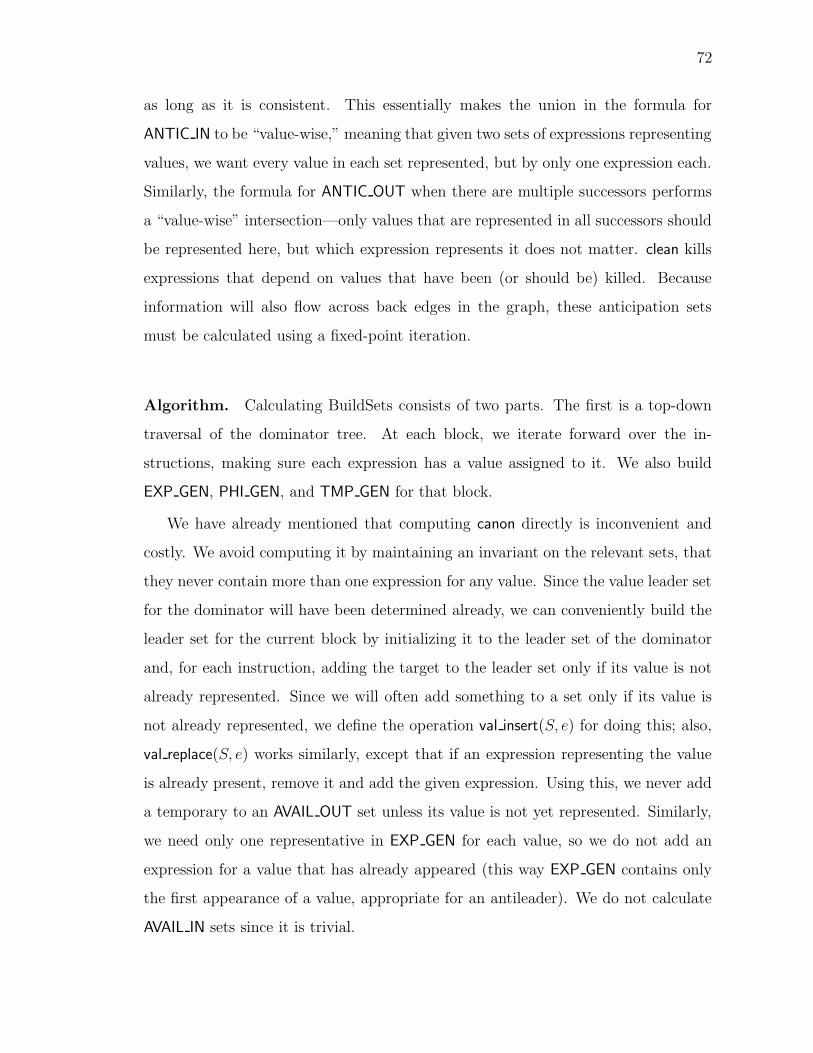
72
as long as it is consistent. This essentially makes the union in the formula for
ANTIC IN to be “value-wise,” meaning that given two sets of expressions representing
values, we want every value in each set represented, but by only one expression each.
Similarly, the formula for ANTIC OUT when there are multiple successors performs
a “value-wise” intersection—only values that are represented in all successors should
be represented here, but which expression represents it does not matter. clean kills
expressions that depend on values that have been (or should be) killed. Because
information will also flow across back edges in the graph, these anticipation sets
must be calculated using a fixed-point iteration.
Algorithm. Calculating BuildSets consists of two parts. The first is a top-down
traversal of the dominator tree. At each block, we iterate forward over the in-
structions, making sure each expression has a value assigned to it. We also build
EXP GEN, PHI GEN, and TMP GEN for that block.
We have already mentioned that computing canon directly is inconvenient and
costly. We avoid computing it by maintaining an invariant on the relevant sets, that
they never contain more than one expression for any value. Since the value leader set
for the dominator will have been determined already, we can conveniently build the
leader set for the current block by initializing it to the leader set of the dominator
and, for each instruction, adding the target to the leader set only if its value is not
already represented. Since we will often add something to a set only if its value is
not already represented, we define the operation val insert(S, e) for doing this; also,
val replace(S, e) works similarly, except that if an expression representing the value
is already present, remove it and add the given expression. Using this, we never add
a temporary to an AVAIL OUT set unless its value is not yet represented. Similarly,
we need only one representative in EXP GEN for each value, so we do not add an
expression for a value that has already appeared (this way EXP GEN contains only
the first appearance of a value, appropriate for an antileader). We do not calculate
AVAIL IN sets since it is trivial.

73
For each block b in a top-down traversal of the dominator treeEXP GEN[b] := PHI GEN[b] := TMP GEN[b] := AVAIL OUT[b] := AVAIL OUT[dom(b)]For each instruction i = t← γ in sequence of b
if γ = φ(t1 . . . tn)add(t, )insert(PHI GEN[b], t)
else if γ = t′
v := lookup(t′)add(t, v)val insert(EXP GEN[b], t′)insert(TMP GEN[b], t)
else if γ = t1 op t2v1 := lookup(t1)v2 := lookup(t2)v := lookup or add(v1 op v2)add(t, v)val insert(EXP GEN[b], t1)val insert(EXP GEN[b], t2)val insert(EXP GEN[b], v1 op v2)insert(TMP GEN[b], t)
else if γ = •v = add(t, )insert(TMP GEN[b], t)
val insert(AVAIL OUT[b], t)
Figure 4.4. First phase of BuildSets
The algorithm for the first phase of BuildSets is in Figure 4.4. In our pseudocode,
we take the liberty of some ML-style notation; for example, if we say “if γ = t”,
we mean “if γ is an instance of a temporary” and “let the variable t stand for that
simple expression in the then clause of this branch.”
The second part calculates flow sets to determine the antileader sets and con-
ducts the fixed-point iteration. Until we conduct a pass on which no ANTIC IN set
changes, we perform top-down traversals of the postdominator tree. This helps fast
convergence since information flows backward over the CFG. The algorithm is given

74
in Figure 4.5. To keep ANTIC IN canonical, we remove the killed temporaries sepa-
rately from ANTIC OUT and EXP GEN, and then do what amounts to a value-wise
union.
Both phi translate and clean process elements in such a way that for any element,
other set elements on which they depend must be processed first. The key to doing
this efficiently is to maintain all sets as topological sorts of the dags they model, which
can be done by implementing the sets as linked lists. Figure 4.6 shows a round of
this process on block 5, including ANTIC IN[B5] before and after the insertions from
S. Notice that the net effect is to replace v7 : t7 in ANTIC OUT with v7 : v3 + v100,
and that although the order has changed, it is still a topological sort.
For this phase to be efficient, the fixed point iteration must converge quickly.
Convergence depends primarily on CFG structure, specifically the number of back
edges and the nesting level of loops. In fact, theoretically, the number of iterations
can be arbitrarily large; for any ε > 0, we can construct a CFG that requires ε
iterations by taking a CFG that requires ε− 1 iterations and adding an extra outer
loop nesting level. In all the code we have compiled, we have found methods in the
virtual machine itself (recall that Jikes RVM is itself written in Java) that required
up to 97 iterations to converge. In normal benchmarks, however, the maximum
number of iterations needed for any method being compiled was 26, and the average
number of rounds needed for methods with more than 5 basic blocks was just over 2.
(Smaller methods were excluded because they tend to be trivial and would artificially
bring down the average.) Moreover, and we found that if we set 10 as the limit, there
was no decrease in the number of operations eliminated in the elimination phase,
implying that the extra rounds needed in extreme cases produce no useful data.
4.3.2 Insert
Insert is concerned with hoisting expressions to earlier program points. If this
phase were skipped, we would be left with a traditional global value numbering
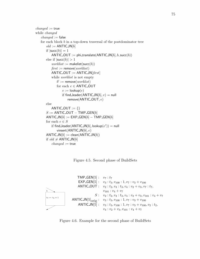
75
changed := true
while changed
changed := false
for each block b in a top-down traversal of the postdominator treeold := ANTIC IN[b]if |succ(b)| = 1
ANTIC OUT := phi translate(ANTIC IN[b], b, succ(b))else if |succ(b)| > 1
worklist := makelist(succ(b))first := remove(worklist )ANTIC OUT := ANTIC IN[first ]while worklist is not empty
b′ := remove(worklist)for each e ∈ ANTIC OUT
v := lookup(e)if find leader(ANTIC IN[b], v) = null
remove(ANTIC OUT, e)else
ANTIC OUT := S := ANTIC OUT− TMP GEN[b]ANTIC IN[b] := EXP GEN[b]− TMP GEN[b]for each e ∈ S
if find leader(ANTIC IN[b], lookup(e′)) = null
vinsert(ANTIC IN[b], e)ANTIC IN[b] := clean(ANTIC IN[b])if old 6= ANTIC IN[b]
changed := true
Figure 4.5. Second phase of BuildSets
5
t7 ← t3 + 1
TMP GEN[5] : v7 : t7EXP GEN[5] : v3 : t3, v100 : 1, v7 : v3 + v100ANTIC OUT : v2 : t2, v3 : t3, v4 : v2 + v3, v7 : t7,
v101 : v4 + v7S : v2 : t2, v3 : t3, v4 : v2 + v3, v101 : v4 + v7
ANTIC IN[5]orig : v3 : t3, v100 : 1, v7 : v3 + v100
ANTIC IN[5] : v3 : t3, v100 : 1, v7 : v3 + v100, v2 : t2,v4 : v2 + v3, v101 : v4 + v7
Figure 4.6. Example for the second phase of BuildSets
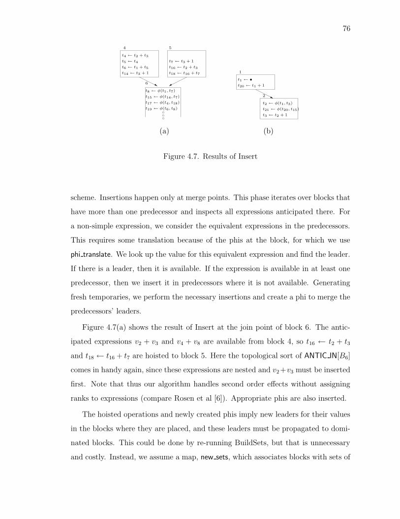
76
t19 ← φ(t6, t8)
t17 ← φ(t4, t18)
t15 ← φ(t14, t7)
t18 ← t16 + t7
t16 ← t2 + t3
t14 ← t3 + 1
t8 ← φ(t1, t7)
t7 ← t3 + 1
t6 ← t1 + t5
t5 ← t4
t4 ← t2 + t3
6
54
t1 ← •
t2 ← φ(t1, t3)
1
2
t3 ← t2 + 1
t20 ← t1 + 1
t21 ← φ(t20, t15)
(a) (b)
Figure 4.7. Results of Insert
scheme. Insertions happen only at merge points. This phase iterates over blocks that
have more than one predecessor and inspects all expressions anticipated there. For
a non-simple expression, we consider the equivalent expressions in the predecessors.
This requires some translation because of the phis at the block, for which we use
phi translate. We look up the value for this equivalent expression and find the leader.
If there is a leader, then it is available. If the expression is available in at least one
predecessor, then we insert it in predecessors where it is not available. Generating
fresh temporaries, we perform the necessary insertions and create a phi to merge the
predecessors’ leaders.
Figure 4.7(a) shows the result of Insert at the join point of block 6. The antic-
ipated expressions v2 + v3 and v4 + v8 are available from block 4, so t16 ← t2 + t3
and t18 ← t16 + t7 are hoisted to block 5. Here the topological sort of ANTIC IN[B6]
comes in handy again, since these expressions are nested and v2+v3 must be inserted
first. Note that thus our algorithm handles second order effects without assigning
ranks to expressions (compare Rosen et al [6]). Appropriate phis are also inserted.
The hoisted operations and newly created phis imply new leaders for their values
in the blocks where they are placed, and these leaders must be propagated to domi-
nated blocks. This could be done by re-running BuildSets, but that is unnecessary
and costly. Instead, we assume a map, new sets, which associates blocks with sets of

77
expressions which have been added to the value leader sets during Insert. Whenever
we create a new computation or phi, we possibly make a new value, and we at least
create a new leader for that value in the given block. We update that block’s leader
set and its new set. Since this information should be propagated to other blocks
which the new temporaries reach, for each block we also add all the expressions in
its dominator’s new set into the block’s own leader set and new set. This also re-
quires us to make Insert a top-down traversal of the dominator tree, so that a block’s
dominator is processed before the block itself.
What we have said so far, however, is not completely safe in the sense that it in
some cases it will lengthen a computational path by inserting an instruction without
allowing one to be eliminated by the next phase. Since v3 + v100 is also anticipated
in at block 6, being anti-inherited from t3 ← t2 + 1 in block 2, we insert t14 ← t3 + 1
in block 4, as shown in Figure 4.7(a). This does not allow any eliminations, but only
lengthens any trace through block 4. The value is still not available at the instruction
that triggered this in block 1 because block 1 was visited first, at which time it was
available on no predecessors and therefore not hoisted. To fix this, we repeat the
process until we make a pass where nothing new is added to any new set. On the
next pass, v7 : t15 is available in block 6, so we hoist t1 + 1 to block 1, as shown
in Figure 4.7(b). In practice, Insert converges quickly. On most benchmarks, the
maximum number of required rounds for any method was 3, and on average it took
only a single round. Note that we do not need predicates for determining latest and
earliest insertion points, since insertions naturally float to the right place. Insertions
made too late in the program will themselves become redundant and eliminated in
the next phase. Figures 4.8 and 4.9 show the algorithm for Insert.
4.3.3 Eliminate
Eliminate is straightforward. For any instruction, find the leader of the target’s
value. If it differs from that target, then there is a constant or an earlier-defined
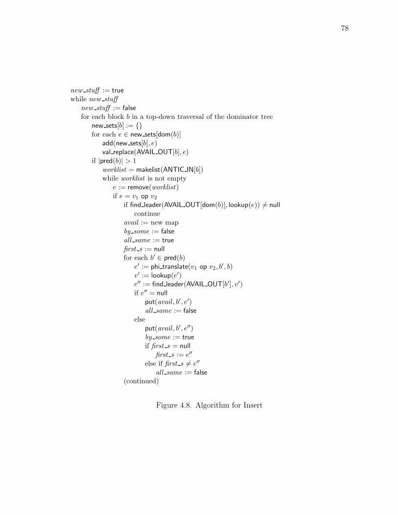
78
new stuff := true
while new stuff
new stuff := false
for each block b in a top-down traversal of the dominator treenew sets[b] := for each e ∈ new sets[dom(b)]
add(new sets[b], e)val replace(AVAIL OUT[b], e)
if |pred(b)| > 1worklist = makelist(ANTIC IN[b])while worklist is not empty
e := remove(worklist)if e = v1 op v2
if find leader(AVAIL OUT[dom(b)], lookup(e)) 6= null
continueavail := new mapby some := false
all same := true
first s := null
for each b′ ∈ pred(b)e′ := phi translate(v1 op v2, b
′, b)v′ := lookup(e′)e′′ := find leader(AVAIL OUT[b′], v′)if e′′ = null
put(avail , b′, e′)all same := false
elseput(avail , b′, e′′)by some := true
if first s = null
first s := e′′
else if first s 6= e′′
all same := false
(continued)
Figure 4.8. Algorithm for Insert
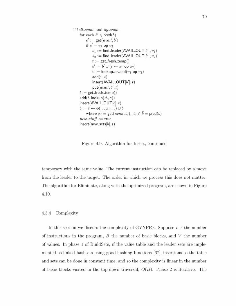
79
if !all same and by some
for each b′ ∈ pred(b)e′ := get(avail , b′)if e′ = v1 op v2
s1 := find leader(AVAIL OUT[b′], v1)s2 := find leader(AVAIL OUT[b′], v2)t := get fresh temp()b′ := b′ ∪ (t← s1 op s2)v := lookup or add(v1 op v2)add(v, t)insert(AVAIL OUT[b′], t)put(avail , b′, t)
t := get fresh temp()add(t, lookup(∆, e))insert(AVAIL OUT[b], t)b := t← φ(. . . xi . . .) ∪ b
where xi = get(avail , bi), bi ∈ b = pred(b)new stuff := true
insert(new sets[b], t)
Figure 4.9. Algorithm for Insert, continued
temporary with the same value. The current instruction can be replaced by a move
from the leader to the target. The order in which we process this does not matter.
The algorithm for Eliminate, along with the optimized program, are shown in Figure
4.10.
4.3.4 Complexity
In this section we discuss the complexity of GVNPRE. Suppose I is the number
of instructions in the program, B the number of basic blocks, and V the number
of values. In phase 1 of BuildSets, if the value table and the leader sets are imple-
mented as linked hashsets using good hashing functions [67], insertions to the table
and sets can be done in constant time, and so the complexity is linear in the number
of basic blocks visited in the top-down traversal, O(B). Phase 2 is iterative. The
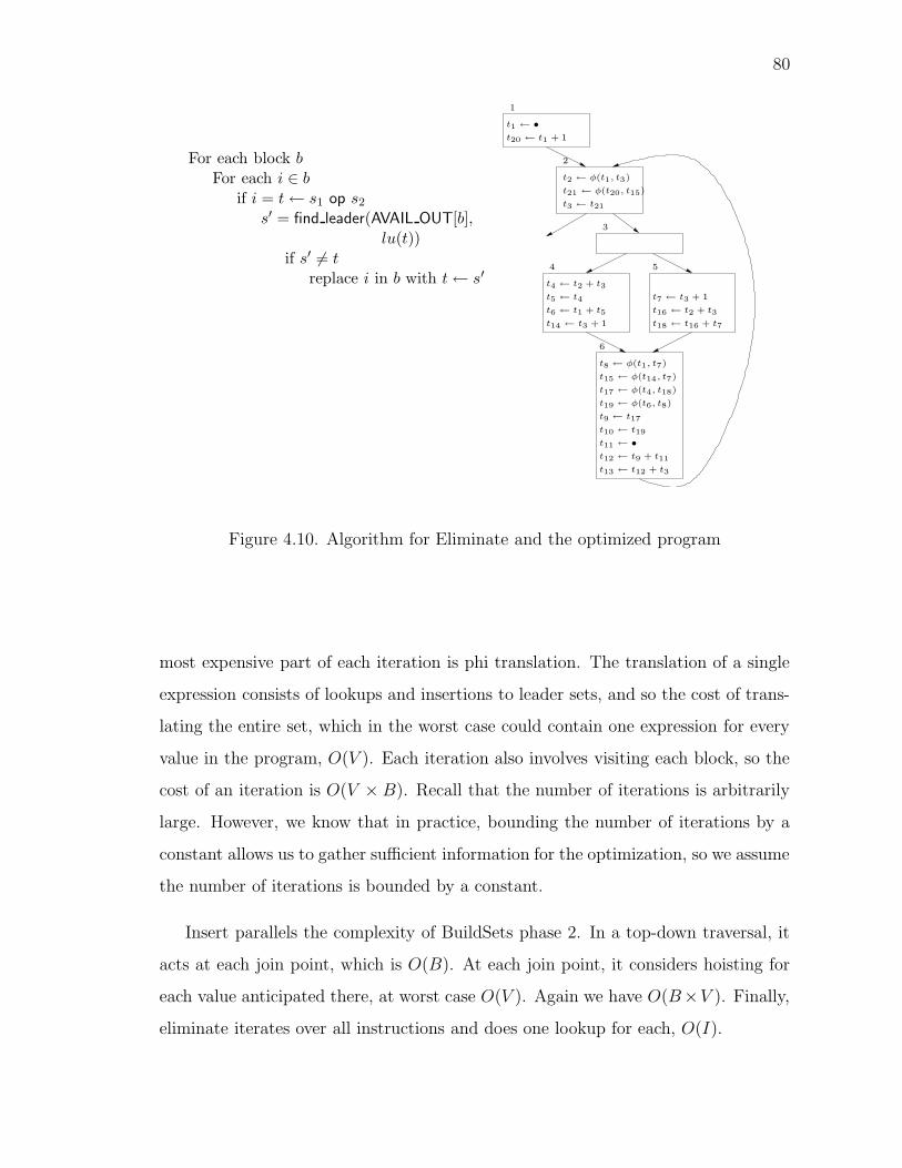
80
For each block bFor each i ∈ b
if i = t← s1 op s2s′ = find leader(AVAIL OUT[b],
lu(t))if s′ 6= t
replace i in b with t← s′
6
t3 ← t21
t4 ← t2 + t3
t5 ← t4
t6 ← t1 + t5
t7 ← t3 + 1
t8 ← φ(t1, t7)
t13 ← t12 + t3
t9 ← t17
t10 ← t19
t11 ← •
t12 ← t9 + t11
t20 ← t1 + 1
t21 ← φ(t20, t15)
t14 ← t3 + 1
t16 ← t2 + t3
t18 ← t16 + t7
t15 ← φ(t14, t7)
t17 ← φ(t4, t18)
t19 ← φ(t6, t8)
5
t1 ← •
t2 ← φ(t1, t3)
1
2
3
4
Figure 4.10. Algorithm for Eliminate and the optimized program
most expensive part of each iteration is phi translation. The translation of a single
expression consists of lookups and insertions to leader sets, and so the cost of trans-
lating the entire set, which in the worst case could contain one expression for every
value in the program, O(V ). Each iteration also involves visiting each block, so the
cost of an iteration is O(V × B). Recall that the number of iterations is arbitrarily
large. However, we know that in practice, bounding the number of iterations by a
constant allows us to gather sufficient information for the optimization, so we assume
the number of iterations is bounded by a constant.
Insert parallels the complexity of BuildSets phase 2. In a top-down traversal, it
acts at each join point, which is O(B). At each join point, it considers hoisting for
each value anticipated there, at worst case O(V ). Again we have O(B×V ). Finally,
eliminate iterates over all instructions and does one lookup for each, O(I).
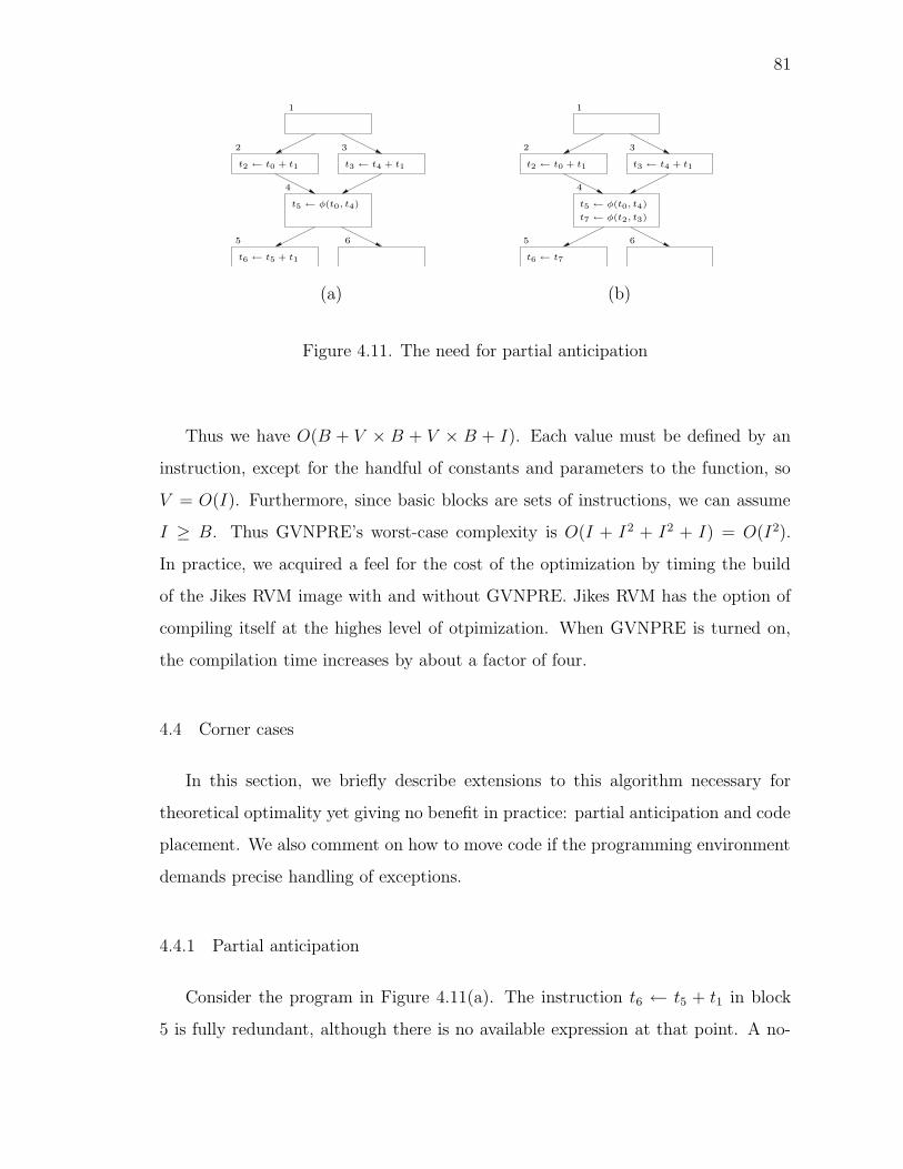
81
65
4
32
1
t6 ← t5 + t1
t5 ← φ(t0, t4)
t3 ← t4 + t1t2 ← t0 + t1
65
4
32
1
t7 ← φ(t2, t3)
t6 ← t7
t5 ← φ(t0, t4)
t3 ← t4 + t1t2 ← t0 + t1
(a) (b)
Figure 4.11. The need for partial anticipation
Thus we have O(B + V × B + V × B + I). Each value must be defined by an
instruction, except for the handful of constants and parameters to the function, so
V = O(I). Furthermore, since basic blocks are sets of instructions, we can assume
I ≥ B. Thus GVNPRE’s worst-case complexity is O(I + I2 + I2 + I) = O(I2).
In practice, we acquired a feel for the cost of the optimization by timing the build
of the Jikes RVM image with and without GVNPRE. Jikes RVM has the option of
compiling itself at the highes level of otpimization. When GVNPRE is turned on,
the compilation time increases by about a factor of four.
4.4 Corner cases
In this section, we briefly describe extensions to this algorithm necessary for
theoretical optimality yet giving no benefit in practice: partial anticipation and code
placement. We also comment on how to move code if the programming environment
demands precise handling of exceptions.
4.4.1 Partial anticipation
Consider the program in Figure 4.11(a). The instruction t6 ← t5 + t1 in block
5 is fully redundant, although there is no available expression at that point. A no-

82
PA OUT =
canonEXP(⋃
b′∈succ(b),¬b′b(ANTIC IN[b′] ∪ PA IN[b′]))
−ANTIC OUT[b] |succ(b)| > 1dep phi trans(PA IN[succ(b)],
ANTIC IN[succ(b)]) |succ(b)| = 1
(4.5)
PA IN[b] = dep clean(canonEXP(PA OUT[b]− TMP GEN[b] (4.6)
−ANTIC IN[b],ANTIC IN[b]))
Other definitions:
dep phi trans(S, S ′, b, b′) = µ′(e, S, S′, b, b′)|e ∈ S (4.7)
µ′(t, S, S′, b, b′) = µ(t, S, b, b′) (4.8)
µ′(v1 op v2, S, S′, b, b′) = lookup(µ′(e1, S, S
′, b, b′)) op lookup(µ′(e2, S, S′, b, b′)), (4.9)
where e1, e2 ∈ S ∪ S′, lookup(e1) = v1,
lookup(e2) = v2
dep clean(S, S ′) = e|e ∈ S, (live(e, S) ∧ live(e, S ′))
(4.10)
Figure 4.12. Flow equations for partial anticipation
cost phi inserted at block 4, however, would allow us to remove that computation.
See Figure 4.11(b). Yet our algorithm as presented so far would not perform this
insertion, because the expression is not anticipated at block 4.
To improve on this, we define partial anticipation. A value is partially anticipated
at a program point if it is computed on at least one but not all paths to program exit.
We define flow equations for calculating PA IN and PA OUT sets for blocks which
are similar to those for ANTIC IN and ANTIC OUT, except that they also depend
on on ANTIC IN and ANTIC OUT, and that PA OUT requires a value-wise union
instead of intersection. The versions of phi translate and clean, called dep phi trans
and dep clean respectively, depend on ANTIC IN. The flow equations and related
definitions are in Figure 4.12.

83
t4 ← t2 + t1
t3 ←
t2 ←
t1 ←
1
t7 ← t6 + t1
43
t8 ← t5 + t1
t6 ← φ(t3, t5)
2
t5 ← φ(t2, t7)
t9 ← t7 + t1
t12 ← φ(t11, t10)
t10 ← φ(t4, t9)
t11 ← t3 + t1
t4 ← t2 + t1
t3 ←
t2 ←
t1 ←
1
t7 ← t12
43
t8 ← t10
t6 ← φ(t3, t5)
2
t5 ← φ(t2, t7)
Figure 4.13. Why partial anticipation is tough
To implement partial anticipation, it would be very inefficient to union all succes-
sor full and partial anticipation sets, then choose canonical representatives, and then
to delete those that are fully anticipated, as the flow equation suggests. Rather, we
iterate through each expression in ANTIC IN and PA IN for each successor, and if the
expression’s value is not already in PA OUT or ANTIC OUT, we add it to PA OUT.
Notice that the flow equation for PA OUT where there is more than one successor
excludes passing partially anticipated expressions across a back edge (that is, when
the successor dominates the block). This is necessary for termination. Consider
the program in Figure 4.13(a). In the body of the loop, a value is incremented
during each iteration, but the result is rotated around t5 and t6, so that the value
from a previous iteration is preserved. The computation t5 + t1 is redundant in all
cases except when the loop body is executed exactly twice: if the loop is executed
only once, its value is stored in t4; if it is executed more than twice, its value was
computed in the third-to-last loop execution. Assuming we name values with the
same numbering as the temporaries which represent them, the expression v5 + v1 is
fully anticipated into block 3. On a first pass, it is not anticipated into block 4, so
it is partially anticipated in block 2. If we were to propagate it across the back edge

84
(4,2), it would become v7 + v1 in block 4, which would require a new value, say v9.
On the next pass, the new value would become partially anticipated in block 2. If we
propagated partial anticipation through the back edge again on the next iteration,
it would become v8 + v1 since v7 is represented by v6 + v1 which maps to v5 + v1,
representing v8. This new expression would again need a new value; this process
would recur infinitely.
Disallowing partial anticipation propagation through a back edge, however, does
not prevent us from identifying and eliminating the redundancy in this case. On the
second pass, block 4 anticipated v5+v1, making that expression now fully anticipated
in block 2. Since it is partially available (t4 from block 1), we insert t9 ← t7 + t1 in
block 4. This insertion makes the value for v6 + v1 partially available, and since it is
fully anticipated at the beginning of block 1, we insert t11 ← t3 + t1 in block 1. The
phis t10 ← φ(t4, t9) and t12 ← φ(t11, t10) allow us to eliminate the computations for
t7 and t8, shortening the single-loop iteration scenario. See Figure 4.13(b).
For Insert, we add an extra step for each join point where we iterate over partially
anticipated expressions. We do not want to make insertions if something is only
partially anticipated, so we create a phi only if the equivalent value exists in all
predecessors We need an extra variable, by all , which we set to false if we inspect a
predecessor where find leader returns null. We insert only if by all is true.
In our experiments on real code, cases like this occur rarely (in one benchmark it
accounted for 3% of the operations eliminated; in seven, 1% or fewer; in ten it never
occurred). PA IN sets also consume much memory, and calculating them increases
the average number of rounds for convergence of BuildSets by an order of magnitude.
4.4.2 Knoop et al’s frontier
Problem
In the categories of Knoop et al [55], our algorithm is code motion, not code
placement, and does not cross the frontier illustrated in Figure 2.2. To extend

85
t6 ← φ(t5, t1)
t7 ← φ(t5, t2)
65
t9 ← t7 + t0t8 ← t6 + t0
t0 ← •
t4 ← t2 + t0
t2 ← •
t1 ← •
1
4
32
t5 ← • t3 ← t1 + t0
4
1
t1 ← •
t2 ← •
t4 ← t2 + t0
t0 ← •
t10 ← t5 + t0
t8 ← t13 t9 ← t12
5 6
t7 ← φ(t5, t2)
t6 ← φ(t5, t1)
t12 ← φ(t10, t4)
t13 ← φ(t10, t3)
3
t5 ← • t3 ← t1 + t0
2
(a) (b)
Figure 4.14. Code placement
this algorithm for code placement, partial anticipation must be used. Our goal is
to eliminate redundant computations without introducing spurious computations.
Therefore as our algorithm makes changes in the program, we make sure never to
lengthen any program path by a computation, though we may lengthen it by moves
and phis. So far, our rule for merging values (or leaders of the same value) in a
phi is that such a merge is appropriate at a join point either if the corresponding
expression is fully anticipated and at least partially available or if it is at least
partially anticipated and fully available. In the former case, we are assured that
any insertion we may need to make will allow an elimination later in all paths from
that point. In the latter case, we are assured that no insertions of computations are
necessary.
Although this approach is safe, it is not complete, which we see as we again turn
to the frontier case. Consider the program in Figure 4.14(a). At the join point in
block 3, the expression t6 + t0 is partially anticipated. It is available from block 2:
translated through the phis, it becomes t1+t0, the leader of whose value is t3. It is not
available in block 1. The expression t7 + t0 is also partially anticipated, and it also is
available from block 2: translated through the phis, it becomes t2 + t0 in block 2, the

86
leader of whose value is t4. It is not available in block 1. Partially anticipated and
partially available, these do not qualify for optimization in the algorithm defined so
far. However, they can be optimized according to our goals. Both of the expressions
translate through the phis to t5 + t0. If we insert that computation in block 1 and
store it in t10, we can use t10 as the operand to two phis, one to merge it with t3
and knock out the computation t6 + t0, the other to merge it with t4 and knock out
t7 + t0. See Figure 4.14(b).
Solution
An enhancement to our algorithm covering these cases is complicated but still
elegant. Consider what is happening at the join point. The computation needed at
the join point is t5 + t0. The question is, should we insert that computation? Since
it is not equivalent to any fully anticipated expression, we know it will not be used
in block 4. Therefore the answer is, it should be inserted if it is used in (all paths
from) block 5 and (all paths from) block 6. How do we know if these will indeed
be used? It will be used on block 5 if we make a phi for t6 + t0; it will be used on
block 6 if we make a phi for t7 + t0. How do we know if we should indeed make
these phis? We should make a phi for a given expression if it is partially available
(which is true in our cases) and is fully hypothetically available (in other words, if
it is already available or will be after safe insertions). Thus an expression at a join
point is “fully hypothetical” if on every predecessor either it is already available or
we will insert a computation for it.
In the words of a children’s song, there is a hole in the bucket. Whether or not
we insert a computation ultimately depends on whether or not we will insert it. To
state the situation formally, suppose π stands for an expression that is partially an-
ticipated and partially available (a “partial-partial”). Let u range over expressions
which would be the right-hand side of hypothetical instructions, possibly to be in-
serted. Suppose that for each partial-partial π, we have a map, µπ, which associates

87
will insert(u) = ∀ s ∈ succ, used(u, s) (4.11)
used(u, s) = ∃ π ∈ µu(s)|make phi(π) (4.12)
make phi(π) = part avail(π) ∧ full hyp(π) (4.13)
part avail(π) = ∃ p ∈ pred|avail(p, π) (4.14)
avail(π, p) = find leader(ANTIC IN[p],
lookup(equivalent expression(succ(p), p, π)))
6= null (4.15)
full hyp(π) = ∀p ∈ pred, avail or hyp(π, p) (4.16)
avail or hyp(π, p) = avail(p, π) ∨ will insert(µπ(p)) (4.17)
(4.18)
Figure 4.15. Predicate system for insertion under partial anticipation
predecessors to expressions for hypothetical instructions. Suppose further that for
each expression for a hypothetical instruction u, we have a map, µu, which asso-
ciates successors with sets of partial-partials. We then have the system of predicates
in Figure 4.15
The system is recursive, and if will insert is true, the recursion will be infinite.
We believe the converse is true. Thus we search for a contradiction to this system,
and consider it to be true if no contradiction is found. In terms of implementation,
will insert should return true if it is reentered for the same argument.
Algorithm
To implement this solution, we need a small change to BuildSets: we need to
build and maintain a map, part succ map, which associates an expression with the
set of blocks on which the partially anticipated expression is fully anticipated but
which are successors to blocks on which it is partially anticipated. Note that this
might not be simply a single block; if a block has three successors and an expression
is anticipated on two of the three, we need to know about both. Thus part succ map

88
is not a simple map associating a key with a single entry but a multi-map associating
a key to a set of entries. Thus we assume another operation on this map, set add,
which takes a map, a key, and an entry; instead of overwriting any older entry for
the given key, it adds that entry to the set of entries for that key.
More needs to be done to Insert. We need a map (hyp map) which will associate
hypothetical computations with maps (µu) from successors to sets of partial-partials,
and a map (part part map) which will associate partial-partials with maps (µπ)
from predecessors to hypothetical computations. While doing insert for partially
anticipated expressions in a given block, if an expression is also partially available
(if it is a partial-partial), take note of it by making a µπ for it; for each predecessor,
µπ should have a simple expression already available or a hypothetical computation
which could be inserted. Each hypothetical computation should have its µu, which
we populate by the successors of the current block found among the blocks at which
the current partial-partial is fully anticipated. After iterating through the partially
anticipated expressions, we consider what hypothetical computations should have
insertions and which partial-partials consequently should phis be made for.
4.4.3 Precise handling of exceptions
Finally, we comment on how to modify this algorithm for the precise handling of
exceptions. The Java programming language [68] requires that the order in which
exceptions are thrown be preserved across transformations of the program. This
means that instructions that could potentially throw an exception may not be re-
ordered. To prevent this, we have to consider any potentially excepting instruction
to kill all potentially excepting expressions when calculating anticipation. To adjust
our algorithm, if a block contains any expression that could throw an exception,
ANTIC OUT should be purged of any potentially excepting expressions before being
used to calculate ANTIC IN. Furthermore, EXP GEN of that block should not include
89
any potentially excepting expressions except for the first that occurs in the block,
since that first such expression kills all others except itself.
4.5 GVNPRE in context
4.5.1 A comparison with Bodık
The contributions of our approach are as follows. First, our analysis considers
larger program chunks than Bodık (basic blocks instead of single instructions). Sec-
ond, we present a framework for expressions and values that takes full advantage
of SSA, completely ignoring source-level lexical constraints and thinking solely in
terms of values and expressions that represent them. Third, no graph is explicitly
constructed nor is any novel structure introduced (contrast with Bodık’s VNG). In-
stead, we achieve the same results by synthesizing well-known tools (SSA, control
flow graphs, value numbers) and techniques (flow equations, liveness analysis, fixed-
point iteration). In fact, our algorithm can be viewed as an extension of a simple
hash-based GVN. Finally, we give an efficient and easily-reproduced implementation
for this algorithm.
4.5.2 A response to our critic
This algorithm was presented in a paper at the Thirteenth International Con-
ference on Compiler Construction [16]. One reviewer, who argued for acceptance,
included comments from an outside reader (who had a penchant for citing SKR
papers [48, 52–54,56]) claiming,
The paper shows an odd understanding of the differences and commonal-
ities of [PRE] and [GVN]. It states that neither PRE nor GVN is strictly
more powerful than the other transformation, and gives evidence for this
thesis by means of an illustrating example. The thesis, however, is wrong.
GVN is strictly more powerful than PRE and encompasses it. The ex-

90
2 3
1
t3 ← t1 + t2
t4 ← t1
t5 ← t2 + t4
2 3
1
t3 ← t1 + t2
t4 ← t1
t5 ← t3
(a) Unoptimized (b) Optimized
Figure 4.16. Why ARWZ is not “local.”
ample demonstrates that local value numbering (LVN), i.e., inside of a
basic block, and PRE, a global program transformation, do not cover
each other. [69]
The implication is that the comparison is not only wrong but banal—of course
a local transformation is weaker than a global one. However, the survey of relevant
literature in Chapter 2 shows that the source of confusion here lies in how ARWZ
and SKR differ on what GVN should be. The “odd understanding” of GVN is the
understanding of a highly published body of literature [38, 41, 44, 51, 57] and the
standard advanced compilers textbook [47]. To be fair, Muchnick does compare
PRE with what he calls “value numbering,” not “global value numbering” [47], but
referring to that notion of value numbering as local or suggesting that it works only
within a basic block is wrong. If a value is computed in a block and recomputed
in a block dominated by the first, the latter computation ought to be removed in
the ARWZ view, because there is a value redundancy that is a full redundancy, as
illustrated in Figure 4.16. This is clearly inter-block and hence legitimately can be
called global. The weakness of ARWZ GVN is that it does not consider partial
redundancies nor do hoisting, and that is what GVNPRE remedies.
91
The critic went on to claim
[T]he authors [sic] conclusion “This (paper) demonstrates that perform-
ing PRE as an extension of GVN can be done simply from a software
engineering standpoint, and that it is feasible as a phase of an optimizing
compiler” has been known for more than 15 years. [69]
Fifteen years implies Steffen’s original SKR paper at TAPSOFT’87 [48]. Besides
the fact that even some of the latest SKR papers are not exactly implementation-
oriented [55], they also concede “major obstacles opposing to its widespread usage
in program optimization” [52]. GVNPRE, on the other hand, is synthesized from
known and widely-used tools and algorithms.
4.5.3 GVNPRE and GCC
From a software engineering perspective, GVNPRE has had something of a suc-
cess story as a compiler phase implemented in the GNU Compiler Collection [70].
Dan Berlin, a researcher at IBM’s T.J. Watson Research Center, wrote,
Having gone through hell implementing and maintaining SSAPRE (it’s
also over 3000 lines of code), I looked upon the relative simplicity of
GVN-PRE with glee. In fact, I’m considering implementing it. . . [67]
After working on the proposed implementation, he said,
. . . I’d like to point out that my GVN-PRE implementation can already
properly rebuild GCC with itself turned on. It took me almost 2 years
to do this with SSAPRE due to the hard-to-understand nature of it.
Thanks a bunch for making my life easier. [67]
4.6 Experiments
Our experiments use Jikes RVM [7–9], a virtual machine that executes Java class-
files. We have implemented the algorithm described here as a compiler phase for the

92
_201
_com
pres
s
_202
_jess
_205
_ray
trace
_213
_java
c
_222
_mpe
gaud
io
_227
_mtrt
Gr−Cry
pt
Gr−Eule
r
Gr−SOR
Gr−FFT
Gr−Hea
pSor
t
Gr−LU
Fact
Gr−M
olDyn
Gr−Ray
Trace
r
Gr−Sea
rch
Gr−Ser
ies
Gr−Spa
rseM
atm
ult
J−BH
J−BiS
ort
J−Em
3d
J−Hea
lth
J−M
ST
J−Per
imet
er
J−Pow
er
J−TSP
J−Tre
eAdd
0.00
1.00
2.00
3.00
4.00
5.00
6.00
7.00
Num
ber
of e
limin
atio
ns (
norm
aliz
ed)
GCSE GVNPREBOTH
Figure 4.17. Static eliminations
optimizing compiler and configured Jikes RVM version 2.3.0 to use the optimizing
compiler only and a generational mark-sweep garbage collector. The optimizing
compiler performs a series of code transformations on both SSA and non-SSA rep-
resentations. It already has global common subexpression elimination (GCSE) in
SSA, which relies on GVN. Placing our phase before these two shows that GVNPRE
completely subsumes GCSE in practice. (Jikes RVM’s LICM is not used because it
performs unsafe speculative motion and forward propagation which GVNPRE does
not.) GCSE is equivalent to GVN as it is presented in this dissertation.
Figure 4.17 shows static eliminations performed by each optimization level. The
left column in each set represents the number of intermediate representation oper-
ations eliminated by GCSE normalized to one, and the second those eliminated by
GVNPRE. In each case, GVNPRE eliminates more, sometimes over six times as
much, although the optimization also inserts operations and in some cases may later
eliminate an operation it has inserted. The third bar shows the number of GVNPRE
eliminations plus the number of operations GCSE can eliminate after GVNPRE has

93
run. Apart from a sprinkling of cases where GCSE picks up an instruction or two,
perhaps the by-product of other transformations on the IR, GCSE does nothing in
addition to GVNPRE.
Our performance results are in Figures 4.18 and 4.19. The runs shown in Figure
4.18 were executed on a 733 MHz Power Macintosh with 32Kb I cache, 32Kb D
cache, and 256K L2 cache running Macintosh OS X. Those in Figure 4.19 were
executed on a 1600MHz Intel Pentium III with 512 MB of RAM and 256 KB cache,
running Red Hat Linux. We use three sets of benchmarks: six from the SPECjvm98
suite [11], eleven from the sequential benchmarks of the Java Grande Forum [13],
and nine from the JOlden Benchmark Suite [14]. (Some benchmarks from these
suites were omitted for implementation issues.) As in Chapter 3, we time only the
running of the application (not compilation), and take the best of ten runs. First
we considered the benchmarks run with Jikes RVM’s O2 optimization level stripped
down so that load elimination (to be addressed in the next chapter), global common
subexpression elimination, and loop invariant code motion are turned off. This
is our baseline. The three bars represent the results of three optimization levels
normalized to our baseline: GCSE, like our baseline except with global common
subexpression elimination turned on; GVNPRE, like our baseline except with the
algorithm presented here turned on; and BOTH, with global common subexpression
elimination, loop invariant code motion, and GVNPRE turned on. We also show the
geometric mean.
On the Macintosh, these optimizations consistently made a modest improvement
on almost all benchmarks, with our GVNPRE having a slight edge. However, on
the Pentium we note that results are mixed for all optimization levels; often the
optimizations make hardly any impact, and sometimes even degradation is incurred.
The most obvious reason is that by keeping a value in a variable to eliminate a later
computation, we could be increasing the live range of that variable (or even intro-
ducing a new one). The increase of register pressure could result in more register
spills at compile time and therefore more memory access at run time. A write and

94
_201
_com
pres
s
_202
_jess
_205
_ray
trace
_222
_mpe
gaud
io
_227
_mtrt
Gr−Cry
pt
Gr−SOR
Gr−FFT
Gr−Hea
pSor
t
Gr−LU
Fact
Gr−M
olDyn
Gr−Ray
Trace
r
Gr−Sea
rch
Gr−Ser
ies
Gr−Spa
rseM
atm
ult
J−BH
J−BiS
ort
J−Em
3d
J−Hea
lth
J−M
ST
J−Per
imet
er
J−Pow
er
J−TSP
J−Tre
eAdd
Geom
etric
mea
n0.00
1.00E
xecu
tion
time
(nor
mal
ized
)
GCSEGVNPREBOTH
Figure 4.18. Performance results on PowerPC
_201
_com
pres
s
_202
_jess
_205
_ray
trace
_213
_java
c
_222
_mpe
gaud
io
_227
_mtrt
Gr−Cry
pt
Gr−Eule
r
Gr−SOR
Gr−FFT
Gr−Hea
pSor
t
Gr−LU
Fact
Gr−M
olDyn
Gr−Ray
Trace
r
Gr−Sea
rch
Gr−Ser
ies
Gr−Spa
rseM
atm
ult
J−BH
J−BiS
ort
J−Em
3d
J−Hea
lth
J−M
ST
J−Per
imet
er
J−Pow
er
J−TSP
J−Tre
eAdd
Geom
etric
mea
n0.00
1.00
Exe
cutio
n tim
e (n
orm
aliz
ed)
GCSEGVNPREBOTH
Figure 4.19. Performance results on Intel

95
_201
_com
pres
s
_202
_jess
_205
_ray
trace
_213
_java
c
_227
_mtrt
Gr−Cry
pt
Gr−Eule
r
Gr−SOR
Gr−FFT
Gr−Hea
pSor
t
Gr−LU
Fact
Gr−M
olDyn
Gr−Ray
Trace
r
Gr−Sea
rch
Gr−Ser
ies
Gr−Spa
rseM
atm
ult
J−BH
J−BiS
ort
J−Em
3d
J−Hea
lth
J−M
ST
J−Per
imet
er
J−Pow
er
J−TSP
J−Tre
eAdd
Geom
etric
mea
n0.00
1.00
Exe
cutio
n tim
e (n
orm
aliz
ed)
GCSEGVNPREBOTH
Figure 4.20. Performance results for the pseudo-adaptive framework on Intel
subsequent read are more expensive than a simple arithmetic expression. This is es-
pecially critical in cases where the register allocator is tuned more for compile time
performance than run time (such as in linear scan allocation [71], which Jikes RVM
uses) or when the register set is small, such as on the Pentium. Any transformation
that eliminates instructions by reloading the value from a variable (such as GCSE)
may increase live ranges, but doing hoisting (as in GVNPRE) is even more danger-
ous. Notice that GCSE results in serious degradation for BH on the Pentium, but
GVNPRE brings the execution time back down. Conversely, GCSE does not effect
the execution time of TSP, but GVNPRE degrades it.
To explore this further, we focused our attention on frequently executed code.
Jikes RVM contains an adaptive framework which initially compiles all code with
a base compiler, but on the fly observes what methods are “hot” and recompiles
them with an optimizing compiler. We used a “pseudo-adaptive” variation on this
framework which precompiles previously-identified hot methods with optimizations
(in our case, the various optimization levels described above), but base compiles all
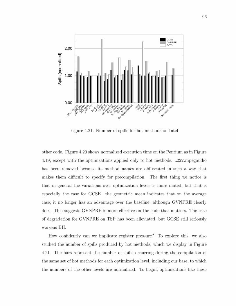
96
_201
_com
pres
s
_202
_jess
_205
_ray
trace
_213
_java
c
_227
_mtrt
Gr−Cry
pt
Gr−Eule
r
Gr−SOR
Gr−FFT
Gr−Hea
pSor
t
Gr−LU
Fact
Gr−M
olDyn
Gr−Ray
Trace
r
Gr−Sea
rch
Gr−Ser
ies
Gr−Spa
rseM
atm
ult
J−BH
J−BiS
ort
J−Em
3d
J−Hea
lth
J−M
ST
J−Per
imet
er
J−Pow
er
J−TSP
J−Tre
eAdd
Geom
etric
mea
n0.00
1.00
2.00
Spi
lls (
norm
aliz
ed)
GCSEGVNPREBOTH
Figure 4.21. Number of spills for hot methods on Intel
other code. Figure 4.20 shows normalized execution time on the Pentium as in Figure
4.19, except with the optimizations applied only to hot methods. 222 mpegaudio
has been removed because its method names are obfuscated in such a way that
makes them difficult to specify for precompilation. The first thing we notice is
that in general the variations over optimization levels is more muted, but that is
especially the case for GCSE—the geometric mean indicates that on the average
case, it no longer has an advantage over the baseline, although GVNPRE clearly
does. This suggests GVNPRE is more effective on the code that matters. The case
of degradation for GVNPRE on TSP has been alleviated, but GCSE still seriously
worsens BH.
How confidently can we implicate register pressure? To explore this, we also
studied the number of spills produced by hot methods, which we display in Figure
4.21. The bars represent the number of spills occurring during the compilation of
the same set of hot methods for each optimization level, including our base, to which
the numbers of the other levels are normalized. To begin, optimizations like these

97
_201
_com
pres
s
_202
_jess
_205
_ray
trace
_213
_java
c
_227
_mtrt
Gr−Cry
pt
Gr−Eule
r
Gr−SOR
Gr−FFT
Gr−Hea
pSor
t
Gr−LU
Fact
Gr−M
olDyn
Gr−Ray
Trace
r
Gr−Sea
rch
Gr−Ser
ies
Gr−Spa
rseM
atm
ult
J−BH
J−BiS
ort
J−Em
3d
J−Hea
lth
J−M
ST
J−Per
imet
er
J−Pow
er
J−TSP
J−Tre
eAdd
Geom
etric
mea
n0.00
1.00
Nor
mal
ized
mem
ory
refe
renc
es
GCSEGVNPREBOTH
Figure 4.22. Number of dynamic memory accesses on Intel
_201
_com
pres
s
_202
_jess
_205
_ray
trace
_213
_java
c
_227
_mtrt
Gr−Cry
pt
Gr−Eule
r
Gr−SOR
Gr−FFT
Gr−Hea
pSor
t
Gr−LU
Fact
Gr−M
olDyn
Gr−Ray
Trace
r
Gr−Sea
rch
Gr−Ser
ies
Gr−Spa
rseM
atm
ult
J−BH
J−BiS
ort
J−Em
3d
J−Hea
lth
J−M
ST
J−Per
imet
er
J−Pow
er
J−TSP
J−Tre
eAdd
Geom
etric
mea
n0.00
1.00
Ret
ired
inst
ruct
ions
(no
rmal
ized
) GCSEGVNPREBOTH
Figure 4.23. Number of retired instructions on Intel

98
_201
_com
pres
s
_202
_jess
_205
_ray
trace
_213
_java
c
_227
_mtrt
Gr−Cry
pt
Gr−Eule
r
Gr−SOR
Gr−FFT
Gr−Hea
pSor
t
Gr−LU
Fact
Gr−M
olDyn
Gr−Ray
Trace
r
Gr−Sea
rch
Gr−Ser
ies
Gr−Spa
rseM
atm
ult
J−BH
J−BiS
ort
J−Em
3d
J−Hea
lth
J−M
ST
J−Per
imet
er
J−Pow
er
J−TSP
J−Tre
eAdd
Geom
etric
mea
n0.00
1.00
Dat
a re
ad m
isse
s (n
orm
aliz
ed)
GCSEGVNPREBOTH
Figure 4.24. Number of data read misses on Intel
indeed tend to increase spills, often severely, and, looking at the geometric mean,
GVNPRE does so more severely than GCSE. On the other hand, there are cases
where either GCSE or GVNPRE decreases spills. Is the number of spills a predictor
of performance? Not exactly, since there are cases such as Euler where GVNPRE
results in a dramatic increase of spills and yet manages a speedup in Figure 4.20.
However, in cases where there is degradation, we typically also find an increased
number of spills ( 201 compress and 213 javac for GVNPRE and, most strikingly,
BH for GCSE).
We also considered the number of dynamic memory references and number of
retired instructions, and data read misses, as shown in Figures 4.22 and 4.23, respec-
tively. These were obtained using the performance counters available on the Pen-
tium [72], using performance counter codes DATA MEM REFS, INST RETIRED,
and DATA READ MISS, respectively. These were measured for the entire applica-
tion, not just the running of the hot methods (though not for compilation, of course),
but still using the “pseudo-adaptive” framework for determining which methods

99
to opt compile. Although both GCSE and GVNPRE improve memory references
slightly, the results are more sporadic than those for retired instructions. This sug-
gests that while the effect on loads and stores to memory are hard to predict, these
optimizations are indeed decreasing the programs’ computational needs, and GVN-
PRE usually more so than GCSE, as observed in Crypt, Search, BH, Em3d, and
Power. The number of data read misses, however, varies greatly, as shown in Fig-
ure 4.24, although on the average, the more optimized levels reduce the number of
misses.
4.7 Conclusions
We have presented an algorithm in which PRE and GVN are extended into a
new approach that subsumes both, describing it formally as a data flow problem and
commenting on a practical implementation. This demonstrates that performing PRE
as an extension of GVN can be done simply from a software engineering standpoint,
and that it is feasible as a phase of an optimizing compiler. An area of incompleteness
is that this approach does not cover instructions for object and array loads. Such an
extension is the topic of the next chapter.

100

101
5 LOAD ELIMINATION ENHANCED WITH PARTIAL REDUNDANCY
ELIMINATION
What happens to a dream deferred?. . .Maybe it just sagslike a heavy load.
—Langston Hughes
5.1 Motivation
Our experiments on the combined GVNPRE technique showed that performance
improvements were modest at best. A significant restriction on GVNPRE’s power
is that it operates only on simple (for example, arithmetic) operations and not on
loads and stores from memory. As the disparity between processor speed and memory
speed widens, it is becoming more critical to optimize memory access instructions.
The goal of the present chapter is to extend the work in the previous chapter for
object and array loads. This section discusses the challenges of this task.
First, we extend our language to include the bracketed portion of the language
presented in Chapter 1. This includes the getfield (gf) operation and putfield (pf)
instruction, and implies we should also extend the notion of expressions from Chapter
4 for getfields:
e ::= . . . | gf x v Expressions
x ranges over field names. The expression corresponds to the getfield operation.
There is no expression for putfields since a putfield does not generate a value but a
side effect. However, if t1 and t2 have values v1 and v2, respectively, an instruction like
pf x t1 t2 implies that the expression gf x v1 has value v2, even if no corresponding
getfield operation appears in the program. We also note that the principles applied

102
t2 ← gf y t1
t1 ← gf x t0
t3 ← gf x t0
t5 ← gf x t0
t6 ← gf y t5
pf y t10 t4
1
2
3
4
5 6
7
t10 ← •
Figure 5.1. Unoptimized program with object references
here to object references can also be applied to array references (which we in fact
do in our implementation and experiments). Instead of a field name and a pointer,
array instructions would have a pointer and an (integer-valued) index.
At first glance, this looks like a simple extension, but in fact it presents a more
difficult problem. Consider the example in Figure 5.1. If we blindly plug the new
language constructs into the old value numbering scheme, we get the value table
shown in Figure 5.2(a) and the transformed program in 5.2(b). This transformation
is wrong because it replaces gf y t5 in block 7 with a reload from t2 which, although
valid, for example, on trace (1,2,7), uses an outdated value for any trace that passes
through block 6, where field y of value v1 is updated. Depending on how careless the
implementation is, it could even determine that t4 and the expression for whatever
operation produced it is also part of the same value, causing further errors.
The essence of the problem is that our SSA assumptions—that any expression
will always have the same static value—do not hold true in the presence of object
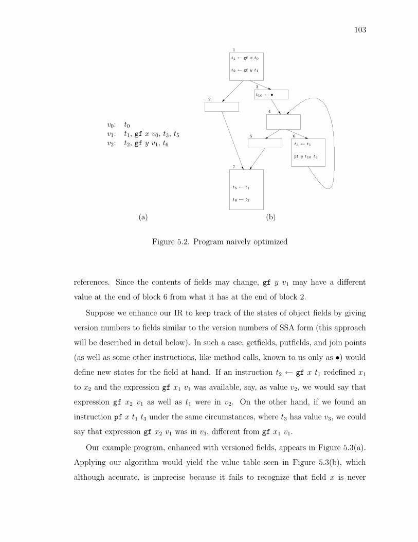
103
v0: t0v1: t1, gf x v0, t3, t5v2: t2, gf y v1, t6
t2 ← gf y t1
t1 ← gf x t0
t3 ← t1
t5 ← t1
t6 ← t2
pf y t10 t4
1
2
3
4
5 6
7
t10 ← •
(a) (b)
Figure 5.2. Program naively optimized
references. Since the contents of fields may change, gf y v1 may have a different
value at the end of block 6 from what it has at the end of block 2.
Suppose we enhance our IR to keep track of the states of object fields by giving
version numbers to fields similar to the version numbers of SSA form (this approach
will be described in detail below). In such a case, getfields, putfields, and join points
(as well as some other instructions, like method calls, known to us only as •) would
define new states for the field at hand. If an instruction t2 ← gf x t1 redefined x1
to x2 and the expression gf x1 v1 was available, say, as value v2, we would say that
expression gf x2 v1 as well as t1 were in v2. On the other hand, if we found an
instruction pf x t1 t3 under the same circumstances, where t3 has value v3, we could
say that expression gf x2 v1 was in v3, different from gf x1 v1.
Our example program, enhanced with versioned fields, appears in Figure 5.3(a).
Applying our algorithm would yield the value table seen in Figure 5.3(b), which
although accurate, is imprecise because it fails to recognize that field x is never
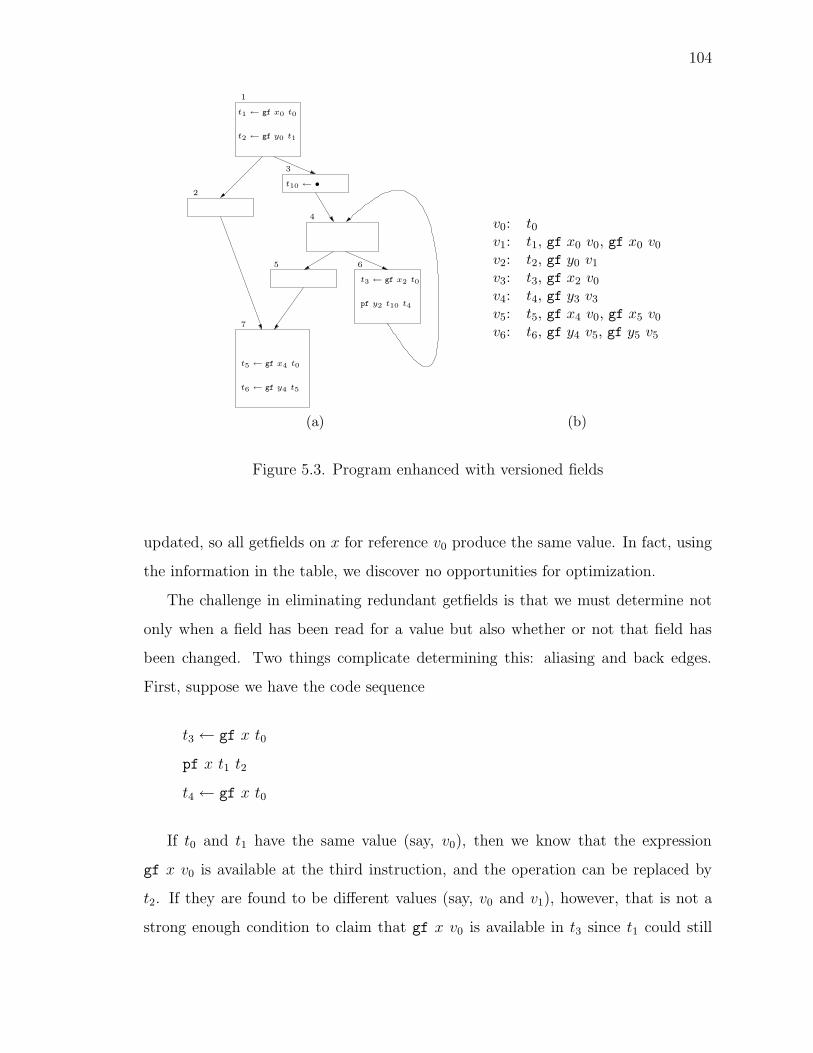
104
t2 ← gf y0 t1
t1 ← gf x0 t0
t3 ← gf x2 t0
t5 ← gf x4 t0
t6 ← gf y4 t5
pf y2 t10 t4
1
2
3
4
5 6
7
t10 ← •
v0: t0v1: t1, gf x0 v0, gf x0 v0v2: t2, gf y0 v1v3: t3, gf x2 v0v4: t4, gf y3 v3v5: t5, gf x4 v0, gf x5 v0v6: t6, gf y4 v5, gf y5 v5
(a) (b)
Figure 5.3. Program enhanced with versioned fields
updated, so all getfields on x for reference v0 produce the same value. In fact, using
the information in the table, we discover no opportunities for optimization.
The challenge in eliminating redundant getfields is that we must determine not
only when a field has been read for a value but also whether or not that field has
been changed. Two things complicate determining this: aliasing and back edges.
First, suppose we have the code sequence
t3 ← gf x t0
pf x t1 t2
t4 ← gf x t0
If t0 and t1 have the same value (say, v0), then we know that the expression
gf x v0 is available at the third instruction, and the operation can be replaced by
t2. If they are found to be different values (say, v0 and v1), however, that is not a
strong enough condition to claim that gf x v0 is available in t3 since t1 could still
105
alias t0; for example, they both could be results of function calls (which would be
represented by • in our language), and dynamically it is possible that the functions
returned the same object reference. In other words, two expressions being in the
same value is a definitely-same (DS) relationship; for precise load optimization, we
also need to know what expressions are in a definitely-different (DD) relationship,
for which we cannot rely on them simply having different values.
Second, knowing what values are the same and available, with any degree of pre-
cision, requires propagating information across back edges. This implies the values
must be calculated using a fixed point iteration rather than a single top-down pass
as in GVNPRE. Fink et al presented a load elimination algorithm (LE) which uses
a fixed point iteration, not to determine value numbers, but to determine, for each
versioned field, what are the values for which the dereference of that field is available,
and to eliminate fully redundant getfields [3]; we describe this algorithm in Section
5.2. Notice that this uses value numbers already computed. However, it handles
only full redundancy; it cannot optimize the instruction t6 ← gf y t5.
What we would like is a value-numbering that discovers in our example that all
references to field x are of the same value, but that this is not true for field y. We
feed this into our GVNPRE which will hoist a getfield for y into block 5. The value
table and the optimized program are shown in Figure 5.4.
How do we calculate this? The pitfall is that we have a chicken-and-egg problem.
In order to partition the expressions into values precisely, we need the results of
the fixed point iteration, but to do the fixed point iteration, we need global value
numbers. It is not a simple thing to let the fixed point iteration refine the value
table, since merging values is a difficult thing to do in a hashing value numbering:
the entire hash table would have to be traversed to update all the references to
the values that have been merged. Furthermore, for expressions to have values as
subexpressions requires values to be stable. Value-numbering schemes that split
congruence classes, such as that in Chapter 3 of Simpson’s dissertation [45], are not
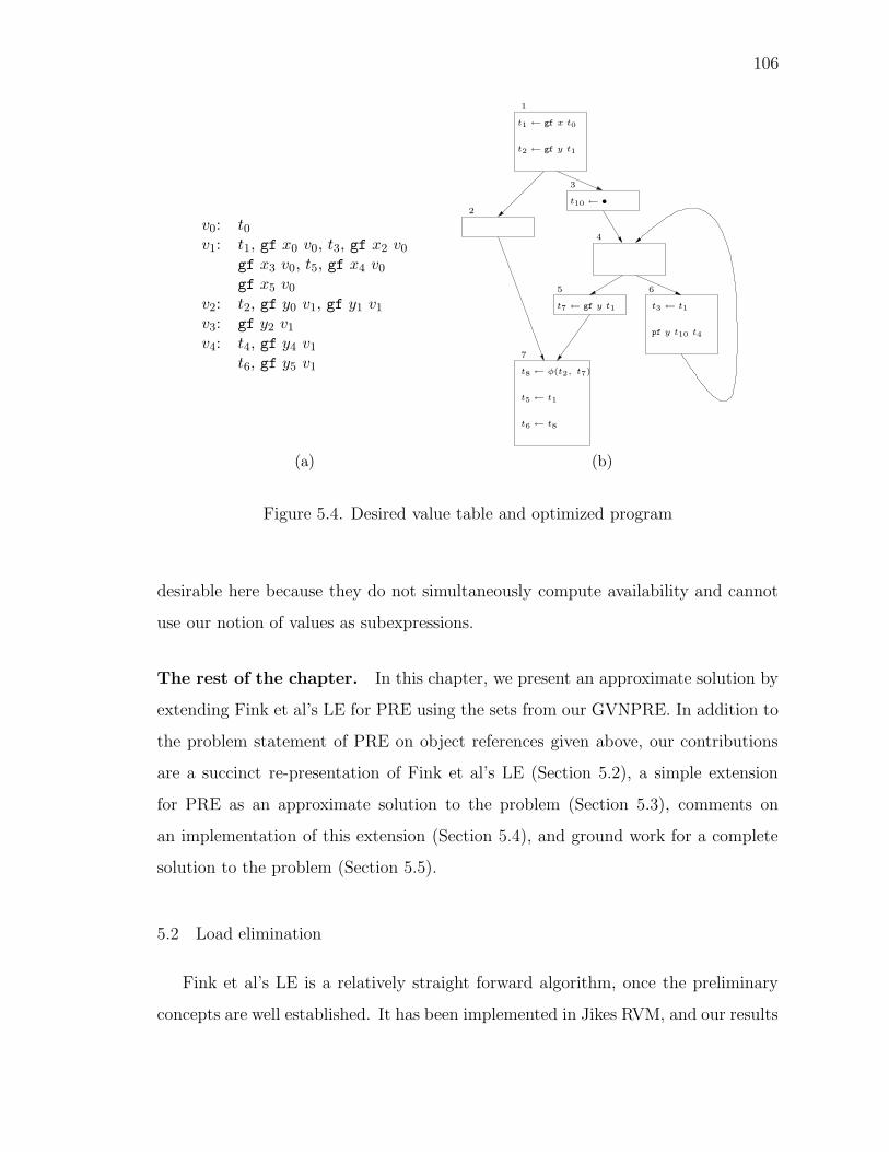
106
v0: t0v1: t1, gf x0 v0, t3, gf x2 v0
gf x3 v0, t5, gf x4 v0gf x5 v0
v2: t2, gf y0 v1, gf y1 v1v3: gf y2 v1v4: t4, gf y4 v1
t6, gf y5 v1
t1 ← gf x t0
t3 ← t1
t5 ← t1
t6 ← t8
pf y t10 t4
1
2
3
4
5 6
7
t7 ← gf y t1
t8 ← φ(t2, t7)
t10 ← •
t2 ← gf y t1
(a) (b)
Figure 5.4. Desired value table and optimized program
desirable here because they do not simultaneously compute availability and cannot
use our notion of values as subexpressions.
The rest of the chapter. In this chapter, we present an approximate solution by
extending Fink et al’s LE for PRE using the sets from our GVNPRE. In addition to
the problem statement of PRE on object references given above, our contributions
are a succinct re-presentation of Fink et al’s LE (Section 5.2), a simple extension
for PRE as an approximate solution to the problem (Section 5.3), comments on
an implementation of this extension (Section 5.4), and ground work for a complete
solution to the problem (Section 5.5).
5.2 Load elimination
Fink et al’s LE is a relatively straight forward algorithm, once the preliminary
concepts are well established. It has been implemented in Jikes RVM, and our results

107
section in this chapter (Section 5.4) shows its impact. The original presentation is
difficult to digest [3]. We give here what we believe to be a simplified explanation,
one that is also amenable to the extension we have in mind. This section contains
clarifications of the preliminary concepts, the algorithm, and a brief discussion.
5.2.1 Preliminaries
LE requires three things: an IR that captures field states, GVN, and alias anal-
ysis.
To capture field states, Fink et al developed an extension of SSA called Extended
Array SSA (EASSA) form [3], based on an earlier extension by Knobe and Sarkar [40].
Field names are given version numbers like variables in SSA form. These versioned
fields are called heap variables. Understanding heap variables requires inverting the
natural way to think of objects and their fields. Normally, we would think of field
references as being “object-major”: first we find the object in memory, and then
search for the appropriate field in that object. For an instruction pf x t1 t2, one
might say, “we are writing to the object to which t1 points, specifically the field x
of that object.” A heap variable view is “field-major”: first we identify the field in
question and then consider which is the relevant object. For the above instruction,
we would say, “we are writing to the field x, specifically that field in the object to
which t1 points.” The distinction is important because we track how the state of the
field changes (across all objects having such a field) rather than how an object (as a
collection of fields) changes.
New field states are defined by variations on the phi functions of SSA. EASSA
uses three types of phis for field states. The first, control phis, merge states at join
points just as SSA phis do, and they will appear the same way in our examples.
Second, use phis introduce a new field state after a read from a field; these appear
in code examples as uφ, and they take the previous state as an argument. Finally,
definition phis introduce a new field state after a write to a field; they appear in

108
pf y2 t10 t4
1
2
3
4
5 6
7
x1 ← uφ(x0)
y1 ← uφ(y0)
x2 ← φ(x1, x3)
y2 ← φ(y0, y3)
x3 ← uφ(x2)
y3 ← dφ(y1)
x4 ← φ(x1, x2)
y4 ← φ(y0, y2)
x5 ← uφ(x4)
y5 ← uφ(y4)
t10 ← •
t6 ← gf y4 t5
t2 ← gf y0 t1
t1 ← gf x0 t0
t3 ← gf x2 t0
t5 ← gf x4 t0
Figure 5.5. Program in Extended Array SSA form
code as dφ, and they take the previous state as an argument. See our example,
unoptimized, translated into EASSA form in Figure 5.5, and compare it with Figure
5.3(a).
LE also needs a value-numbering scheme that gives a value (or value number) for
any variable name. The lookup function of GVNPRE will do nicely. One optimization
level discussed in Section 5.4 shows the results of feeding GVNPRE into an LE
implementation originally designed for an ARWZ GVN.
Finally there must be available information to determine DD and DS . The
original LE presentation considered these to be predicates over variable names, but
considering them to be predicates on values works just as well, since that reduces
DS to equality. DD is tricky, in particular because it is not an equivalence relation.
Precise determination is impossible statically, so we assume each pair of values is
definitely different unless proven otherwise. Fink et al give two observations for
determining two values to be different:
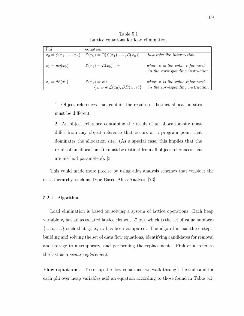
109
Table 5.1Lattice equations for load elimination
Phi equation
x0 = φ(x1, . . . , xn) L(x0) = u(L(x1), . . . ,L(xn)) Just take the intersection
x1 = uφ(x0) L(x1) = L(x0) t v where v is the value referenced
in the corresponding instruction
x1 = dφ(x0) L(x1) = vt where v is the value referenced
w|w ∈ L(x0),DD(w, v) in the corresponding instruction
1. Object references that contain the results of distinct allocation-sites
must be different.
2. An object reference containing the result of an allocation-site must
differ from any object reference that occurs at a program point that
dominates the allocation site. (As a special case, this implies that the
result of an allocation site must be distinct from all object references that
are method parameters). [3]
This could made more precise by using alias analysis schemes that consider the
class hierarchy, such as Type-Based Alias Analysis [73].
5.2.2 Algorithm
Load elimination is based on solving a system of lattice operations. Each heap
variable xi has an associated lattice element, L(xi), which is the set of value numbers
. . . vj . . . such that gf xi vj has been computed. The algorithm has three steps:
building and solving the set of data flow equations, identifying candidates for removal
and storage to a temporary, and performing the replacements. Fink et al refer to
the last as a scalar replacement.
Flow equations. To set up the flow equations, we walk through the code and for
each phi over heap variables add an equation according to those found in Table 5.1.
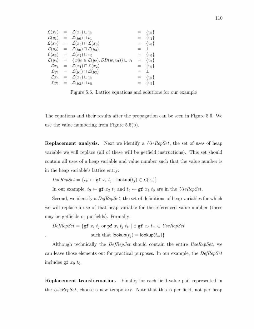
110
L(x1) = L(x0) t v0 = v0L(y1) = L(y0) t v1 = v1L(x2) = L(x0) u L(x3) = v0L(y2) = L(y0) u L(y3) = ⊥L(x3) = L(x2) t v0 = v0L(y3) = w|w ∈ L(y2),DD(w, v3) t v1 = v3Lx4 = L(x1) u L(x2) = v0Ly4 = L(y1) u L(y2) = ⊥Lx5 = L(x3) t v0 = v0Ly5 = L(y3) t v5 = v5
Figure 5.6. Lattice equations and solutions for our example
The equations and their results after the propagation can be seen in Figure 5.6. We
use the value numbering from Figure 5.5(b).
Replacement analysis. Next we identify a UseRepSet , the set of uses of heap
variable we will replace (all of these will be getfield instructions). This set should
contain all uses of a heap variable and value number such that the value number is
in the heap variable’s lattice entry:
UseRepSet = tk ← gf xi tj | lookup(tj) ∈ L(xi)
In our example, t3 ← gf x2 t0 and t5 ← gf x4 t0 are in the UseRepSet .
Second, we identify a DefRepSet , the set of definitions of heap variables for which
we will replace a use of that heap variable for the referenced value number (these
may be getfields or putfields). Formally:
DefRepSet = gf xi tj or pf xi tj tk | ∃ gf x` tm ∈ UseRepSet
. such that lookup(tj) = lookup(tm)
Although technically the DefRepSet should contain the entire UseRepSet , we
can leave those elements out for practical purposes. In our example, the DefRepSet
includes gf x0 t0.
Replacement transformation. Finally, for each field-value pair represented in
the UseRepSet , choose a new temporary. Note that this is per field, not per heap
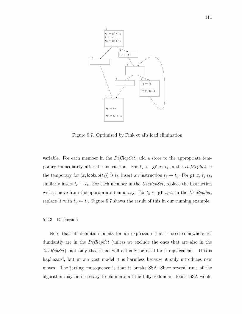
111
t1 ← gf x t0
t3 ← t7
t5 ← t7
t6 ← gf y t5
pf y t10 t4
1
2
3
4
5 6
7
t7 ← t1
t10 ← •
t2 ← gf y t1
Figure 5.7. Optimized by Fink et al’s load elimination
variable. For each member in the DefRepSet , add a store to the appropriate tem-
porary immediately after the instruction. For tk ← gf xi tj in the DefRepSet, if
the temporary for (x, lookup(tj)) is t`, insert an instruction t` ← tk. For pf xi tj tk,
similarly insert t` ← tk. For each member in the UseRepSet , replace the instruction
with a move from the appropriate temporary. For tk ← gf xi tj in the UseRepSet ,
replace it with tk ← t`. Figure 5.7 shows the result of this in our running example.
5.2.3 Discussion
Note that all definition points for an expression that is used somewhere re-
dundantly are in the DefRepSet (unless we exclude the ones that are also in the
UseRepSet), not only those that will actually be used for a replacement. This is
haphazard, but in our cost model it is harmless because it only introduces new
moves. The jarring consequence is that it breaks SSA. Since several runs of the
algorithm may be necessary to eliminate all the fully redundant loads, SSA would
112
have to be rebuilt. The root of the problem is that the algorithm regresses to lexical
equivalence since it groups expressions by a form of lexical similarity (whether they
are in the form gf x t, as long as each t is in the same value), not by the static value
they compute, and then assigns a variable name to that group. To preserve SSA,
each expression in the group would require its own variable (which would actually
be unnecessary, considering each would be part of a value that already has a leader
that is a variable or constant), and we would need to collect the relevant join points
for placing of new phis to merge these variables.
5.3 LEPRE
We come now to the main portion of the chapter. We present a simple extension
to Fink et al’s load elimination to cover cases where a load is partially redundant.
The essence of the idea is to let the lattice equations for phis compute a union rather
than an intersection; since we will hoist instructions to predecessors where a certain
value is not available, we want to consider a value available at a phi if it is available
on at least one predecessor. However, that is not enough for safe code motion,
because we will make such insertions only if the value is fully anticipated at that
program point, that is, it will be used in a replacement on all paths to program exit.
Unfortunately, expanding the DefRepSet to include phis only gives us single-path
anticipation (the value is anticipated somewhere), not all-paths anticipation, which
we want. To accommodate this, we must extend EASSA form and compute a second
lattice for anticipation; the two lattices will interact.
5.3.1 Extending EASSA
Phis are useful to mark places where availability merges. Since anticipation is the
backward-flow analogue of availability, merge points for anticipation are the branch
points in forward flow of the program. To capture the merging of anticipation, we
introduce a new construct, a psi, which is placed on branch points in the CFG.

113
1
32
x1 valid here
x2 valid here x3 valid here
x2, x3 ← ψ(x1) L′(x1) = L′(x2) u L′(x3)
L(x2) = L(x1)L(x3) = L(x1)
Figure 5.8. Psi illustrated
The psi takes as an argument the current heap variable for a field and returns
a set of new heap variables (new versions for the field), one for each successor.
See the example in Figure 5.8. Building EASSA this way is simple; in a practical
EASSA implementation, there are already other kinds of instructions that require
the definitions of heap variables for all valid fields (calls, for example); all we need
to do is include basic block headers among those instructions that rename all valid
fields.
5.3.2 Lattice operations
The modified lattice operations are in Table 5.2. To account for this new variety
of “phi,” we need an extra kind of flow equation for the original lattice. A psi simply
propagates the current value numbers from its argument’s lattice cell to those of its
definitions, as illustrated by the two equations defining L(x2) and L(x3) in Figure
5.8. In the reverse direction, the value for x1 in the anticipation lattice is defined by
the intersection of the predecessor elements, L′(x2) and L′(x3) in our example. This
works just as phis do for the availability lattice in the original set of equations.
The equations for use phis and def phis are similar to those for the original lattice,
except the flow goes in the opposite direction. In Figure 5.9, the use phi attached
to the getfield adds v1 to the set of values anticipated in the sequent. In the case of

114
x1 valid here
x2 valid here
t2 ← gf x t1
x2 ← uφ(x1)
L′(x1) = v1 t L′(x2)
Figure 5.9. Illustration of use phi
x2 valid here
21
x3 ← φ(x1, x2)
3
x1 valid here
t3 ← φ(t1, t2)
t4 ← gf x t3
if L′(x3) = v2, then
L′(x1) = phi translate(v3, 3, 1) = v1
L′(x2) = phi translate(v3, 3, 2) = v2
Figure 5.10. Illustration for control phis
a def phi (not shown), we again must purge values not definitely different from the
one used at the given instruction.
Control phis are handled for anticipation just as psis are handled for availabil-
ity, except that the value must be transfered through the phis at the block. In
Figure 5.10, L′(x1) and L′(x2) should be v1 and v2, respectively. The function
phi translate(v3, 3, 1), where b1 is the predecessor that corresponds to t1, returns v1;
similarly with b2, v2. But the most important change is that to control phis for the
original lattice. Here is where the lattices interact. As before, we begin with the
intersection of the lattice elements from the predecessors. In addition, we add any
value that is anticipated (that is, it is present in the heap variable’s other lattice
element) whose translated value is also available on at least one predecessor. We
add a further restriction—on all predecessors the value must transfer to something
that is available. This is so we have the necessary value available if we need to make

115
Table 5.2Additional and revised lattice equations for LEPRE
Phi equationx0 = φ(x1, . . . , xn) L′(xi) = v|∃w ∈ L(x0), where b1, . . . , bn are the predecessors of b
v = phi translate(w, b, bi) corresponding to x1, . . . , xn, respectively
x1 = uφ(x0) L′(x0) = L′(x1) t v where v is the value referenced
in the corresponding instruction
x1 = dφ(x0) L′(x0) = vt where v is the value referenced
w|w ∈ L′(x1),DD(w, v) in the corresponding instruction
x1, . . . , xn = ψ(x0) L′(x0) = uL′(x1) . . .L′(xn) just take the intersection
x0 = φ(x1, . . . , xn) L(x0) = u(L(x1), . . . ,L(xn))tv|v ∈ L′(x0) and where b1, . . . , bn are the predecessors of b
∃L(xi) ∈ L(x1), . . . ,L(xn)such that corresponding to x1, . . . , xn, respectively
phi translate(v, b, bi) ∈ L(xi)and ∀bj ∈ b1, . . . , bn,phi translate(v, b, bj) 6= null
x1, . . . , xn = ψ(x0) L(xi) = L(x0) For i ∈ 1 . . . n
an insertion on any predecessor. Consider the example in Figure 5.11 (we show
the EASSA annotations for the field y only, for brevity). Since L′(y1) = v1 and
L(y2) = v1 (where lookup(t1) = v1), we would say that L(y1) = v1 except that
gf y v1 is not insertable in block 1 since the value v1 has no representative (leader
in our terminology) there. This example also illustrates the need for several rounds
of this optimization (just like the original load elimination), since in the first round,
gf x t0 will be hoisted to block 1, after which the insertion for y will be possible.
5.3.3 Insertion
We must add another phase, between replacement analysis and replacement
transformation, a phase for the insertion of new instructions. For each control phi
x0 ← φ(x1, . . . , xn), we must consider the value numbers in L(x0). For a value num-
ber v, consider if vi ∈ L(xi) for all xi ∈ x1, . . . , xn, where vi = phi translate(v, b, bi)
and bi is the predecessor block corresponding to xi. If vi /∈ L(xj), corresponding to
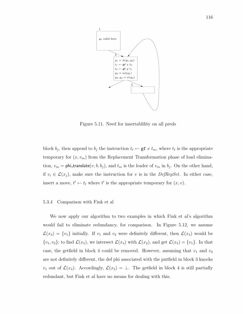
116
3
y3, y4 = ψ(y2)
y0 valid here
y2 = uφ(y1)
t2 ← gf y t1
y1 = φ(y0, y2)
t1 ← gf x t0
2
1
Figure 5.11. Need for insertablility on all preds
block bj, then append to bj the instruction t` ← gf x tm, where t` is the appropriate
temporary for (x, vm) from the Replacement Transformation phase of load elimina-
tion, vm = phi translate(v, b, bj), and tm is the leader of vm in bj. On the other hand,
if vi ∈ L(xj), make sure the instruction for v is in the DefRepSet. In either case,
insert a move, t′ ← t` where t′ is the appropriate temporary for (x, v).
5.3.4 Comparison with Fink et al
We now apply our algorithm to two examples in which Fink et al’s algorithm
would fail to eliminate redundancy, for comparison. In Figure 5.12, we assume
L(x3) = v1 initially. If v1 and v2 were definitely different, then L(x4) would be
v1, v2; to find L(x5), we intersect L(x4) with L(x2), and get L(x5) = v1. In that
case, the getfield in block 4 could be removed. However, assuming that v1 and v2
are not definitely different, the def phi associated with the putfield in block 3 knocks
v1 out of L(x4). Accordingly, L(x5) = ⊥. The getfield in block 4 is still partially
redundant, but Fink et al have no means for dealing with this.
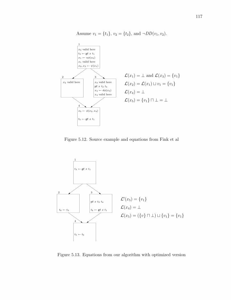
117
Assume v1 = t1, v2 = t2, and ¬DD(v1, v2).
x2, x3 ← ψ(x1)
x0 valid here
x1 valid here
x1 ← uφ(x0)
t3 ← gf x t1
1
x2 valid here
4
32
pf x t2 t4
x4 ← dφ(x3)
t5 ← gf x t1
x5 ← φ(x2, x4)
x4 valid here
x3 valid here
L(x1) = ⊥ and L(x3) = v1
L(x2) = L(x1) t v1 = v1
L(x4) = ⊥
L(x5) = v1 u ⊥ = ⊥
Figure 5.12. Source example and equations from Fink et al
t6 ← gf x t1t6 ← t3
t3 ← gf x t1
1
4
32
pf x t2 t4
t5 ← t6
L′(x5) = v1
L(x4) = ⊥
L(x5) = (v u ⊥) t v1 = v1
Figure 5.13. Equations from our algorithm with optimized version

118
t5 ← φ(t1, t2)
t4 ← gf x t2t3 ← gf x t1
x4 ← uφ(x3)
t6 ← gf x t5
x5 ← φ(x2, x4)
x4 valid here
x3 valid here
x2 valid here
x2 ← uφ(x1)
x1 valid here
3
1 2
L(x2) = v1
L(x4) = v2
L(x5) = v1 u v2 = ⊥
Figure 5.14. Source example and equations from Fink et al
t7 ← t4
t4 ← gf x t2
t7 ← t3
t6 ← t7
t5 ← φ(t1, t2)
t3 ← gf x t1
3
1 2
L′(x5) = v5
L(x5) = (v1 u v2) t v5 = v5
Figure 5.15. Equations from our algorithm with optimized version
Using the algorithm presented in this chapter, we first note that L′(x5) = v1.
Then, since phi translate(v1, 4, 2) = v1 and v1 ∈ L(x2) (that is, the equivalent value
number is available on a predecessor), we find L(x5) = v1. In the insertion stage,
we insert a getfield in block 3 and a move in block 2, allowing us to eliminate the
computation in block 4. See Figure 5.13.
In Figure 5.14, we have an example where Fink et al fails to remove even a
full redundancy. The value equivalent to the instruction gf x t5 has been com-
puted on each path to the occurrence, but since the object reference has a different
value from the one in block 3, Fink et al’s analysis finds L(x5) = ⊥. Using our
algorithm, however, we find L′(x5) = v5, since phi translate(v5, 3, 1) = v1 and
119
phi translate(v5, 3, 2) = v2. In the insertion stage, we insert no computations but
only moves. Then the computation in block 3 can be removed.
5.3.5 A comparison with Bodık
Bodık gives examples that include array accesses [57], but does not discuss alias-
ing. One would assume that value threads would need to be cut when crossing an
instruction that writes to an array that could be the same as the array used in the
current value thread, similar to the provision for ASSAPRE in chi insertion at the
end of Section 3.3.1. Although Bodık’s approach is more precise than the ad hoc
LEPRE, LEPRE has the advantage of using the standard and relatively simple lat-
tice approach instead of the value name graph, and it does not require considering
each instruction as its own basic block.
5.4 Experiments
Our experiments use Jikes RVM [7–9], a virtual machine that executes Java class-
files. We have implemented the algorithm described here as a compiler phase for the
optimizing compiler and configured Jikes RVM version 2.3.0 to use the optimizing
compiler only and a generational mark-sweep garbage collector. The optimizing
compiler performs a series of code transformations on both SSA and non-SSA rep-
resentations. It already has LE.
We use three sets of benchmarks: five from the SPECjvm98 suite [11], ten from
the sequential benchmarks of the Java Grande Forum [13], and seven from the JOlden
Benchmark Suite [14]. First we considered the normal O2 level optimization of Jikes
RVM, with the addition of the GVNPRE algorithm from the previous chapter. This
is our baseline. Our intention is to show the affect of the LEPRE algorithm from
this chapter; however, LEPRE requires a stronger value numbering than the one
provided by Jikes RVM and used by default by LE. So we consider a level called
VNPRELE, which shows the effect of running the old LE except with GVNPRE’s

120
_201
_com
pres
s
_202
_jess
_205
_ray
trace
_222
_mpe
gaud
io
_227
_mtrt
Gr−Cry
pt
Gr−Eule
r
Gr−SOR
Gr−FFT
Gr−Hea
pSor
t
Gr−LU
Fact
Gr−M
olDyn
Gr−Sea
rch
Gr−Ser
ies
Gr−Spa
rseM
atm
ult
J−BiS
ort
J−Em
3d
J−Hea
lth
J−M
ST
J−Per
imet
er
J−TSP
J−Tre
eAdd
0.0
1.0N
umbe
r of
elim
inat
ions
(no
rmal
ized
)
VNPRELELEPRE
Figure 5.16. Static eliminations
value numbering rather than the default. The other level demonstrates the effects of
optimizing a program with LEPRE. Figure 5.16 shows static eliminations performed
by each optimization level, with the first bar representing the number of instructions
eliminated by LE followed by the number eliminated by VNPRELE and LEPRE, all
normalized to the LE level. We make two observations. First, the number of instruc-
tions eliminated changes noticeably by simply giving a smarter value numbering to
old LE. Second, the increase of eliminations when PRE is added is only modest.
There appears to be little opportunity to hoist loads to earlier program points.
Our performance results in Figure 5.17 show runs executed on a 1600MHz In-
tel Pentium 3 with 512 MB of RAM and 256 KB cache, running Red Hat Linux.
Recall from Chapter 4 that optimizations that reload values from temporaries can
have the negative effect of lengthening live ranges and bringing out more spills, and
that hoisting can aggravate this further. However, the extra eliminations using VN-
PRELE appear to have little effect, positive or negative. Not surprisingly, the few
eliminations gained by LEPRE do not affect performance much either.

121
_201
_com
pres
s
_202
_jess
_205
_ray
trace
_222
_mpe
gaud
io
_227
_mtrt
_228
_jack
Gr−Cry
pt
Gr−Eule
r
Gr−SOR
Gr−FFT
Gr−Hea
pSor
t
Gr−LU
Fact
Gr−M
olDyn
Gr−Sea
rch
Gr−Ser
ies
Gr−Spa
rseM
atm
ult
J−BiS
ort
J−Em
3d
J−Hea
lth
J−M
ST
J−Per
imet
er
J−TSP
J−Tre
eAdd
Geom
etric
mea
n0.0
1.0
Exe
cutio
n tim
e (n
orm
aliz
ed)
VNPRELELEPRE
Figure 5.17. Performance results
_201
_com
pres
s
_202
_jess
_205
_ray
trace
_227
_mtrt
Gr−Cry
pt
Gr−Eule
r
Gr−SOR
Gr−FFT
Gr−Hea
pSor
t
Gr−LU
Fact
Gr−M
olDyn
Gr−Sea
rch
Gr−Ser
ies
Gr−Spa
rseM
atm
ult
J−BiS
ort
J−Em
3d
J−Hea
lth
J−M
ST
J−Per
imet
er
J−TSP
J−Tre
eAdd
Geom
etric
mea
n0.0
1.0
2.0
Exe
cutio
n tim
e (n
orm
aliz
ed)
VNPRELELEPRE
Figure 5.18. Performance results for the pseudo-adaptive framework

122
_201
_com
pres
s
_202
_jess
_205
_ray
trace
_227
_mtrt
Gr−Cry
pt
Gr−Eule
r
Gr−SOR
Gr−FFT
Gr−Hea
pSor
t
Gr−LU
Fact
Gr−M
olDyn
Gr−Sea
rch
Gr−Ser
ies
Gr−Spa
rseM
atm
ult
J−BiS
ort
J−Em
3d
J−Hea
lth
J−M
ST
J−Per
imet
er
J−TSP
J−Tre
eAdd
Geom
etric
mea
n0.0
1.0
2.0
3.0
Nor
mal
ized
spi
llsVNPRELELEPRE
Figure 5.19. Number of spills for hot methods
As in Chapter 4, we considered the effect of running these optimizations only
on hot code and measuring both performance and spills, which results appear in
Figures 5.18 and 5.19, respectively. While the extra eliminations do produce more
spills in most benchmarks, they do not appear to translate into a performance hit.
Most benchmarks appear flat apart from the anomalous degradation of Euler, a case
when in fact we reduce the number of spills.
To round out the picture, we also considered the affects on dynamic memory
references, retired instructions, and data read misses, as we did earlier. See Figures
5.20, 5.21, and 5.22. Again, these in the framework where the optimizations are
performed only on the hot methods. Most of these numbers are fairly flat as well, al-
though we do gain insight into the behavior of MolDyn in the LEPRE level. MolDyn
takes a hit even from whole-program optimization in Figure 5.17, which recurs in the
optimization of hot methods in Figure 5.18. We can relate that to increased memory
references and retired instructions. While MolDyn on the LEPRE level does not
increase spills excessively, a few spills in critical areas could cause this degradation.
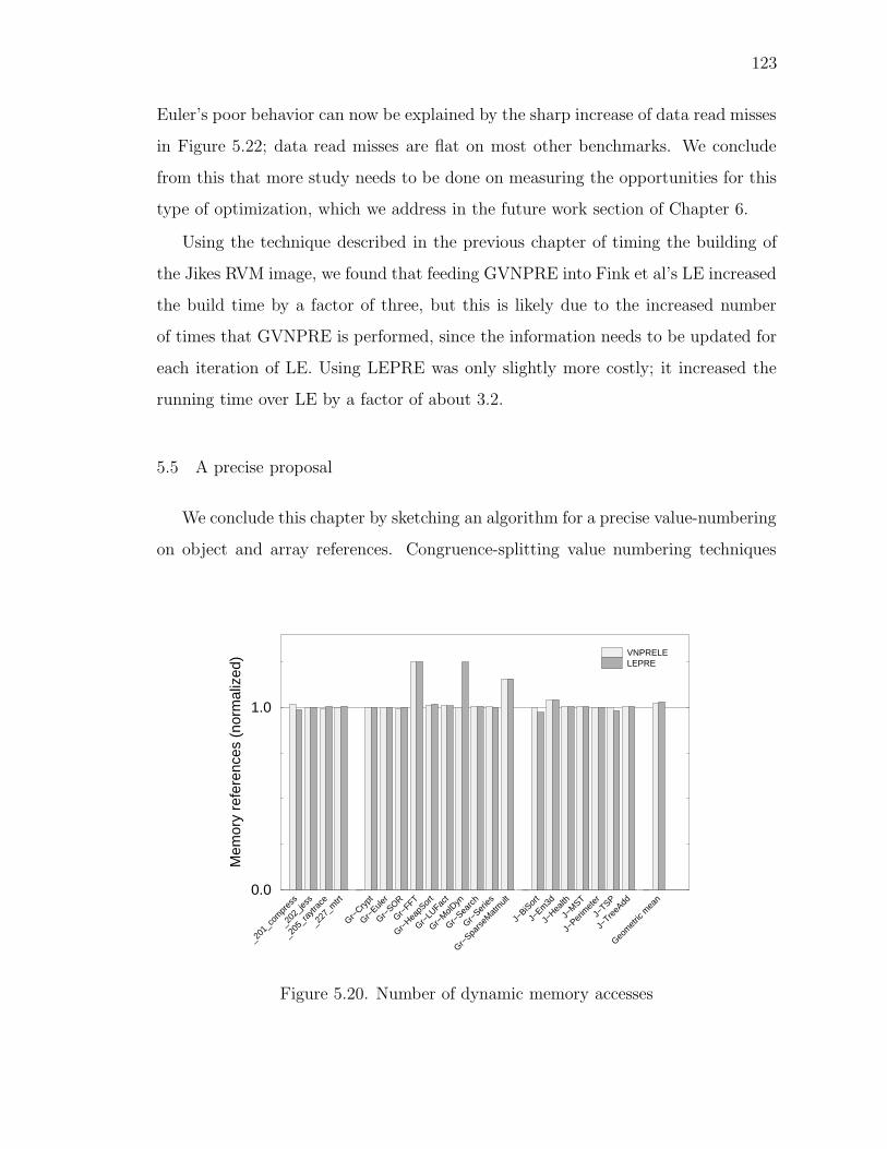
123
Euler’s poor behavior can now be explained by the sharp increase of data read misses
in Figure 5.22; data read misses are flat on most other benchmarks. We conclude
from this that more study needs to be done on measuring the opportunities for this
type of optimization, which we address in the future work section of Chapter 6.
Using the technique described in the previous chapter of timing the building of
the Jikes RVM image, we found that feeding GVNPRE into Fink et al’s LE increased
the build time by a factor of three, but this is likely due to the increased number
of times that GVNPRE is performed, since the information needs to be updated for
each iteration of LE. Using LEPRE was only slightly more costly; it increased the
running time over LE by a factor of about 3.2.
5.5 A precise proposal
We conclude this chapter by sketching an algorithm for a precise value-numbering
on object and array references. Congruence-splitting value numbering techniques
_201
_com
pres
s
_202
_jess
_205
_ray
trace
_227
_mtrt
Gr−Cry
pt
Gr−Eule
r
Gr−SOR
Gr−FFT
Gr−Hea
pSor
t
Gr−LU
Fact
Gr−M
olDyn
Gr−Sea
rch
Gr−Ser
ies
Gr−Spa
rseM
atm
ult
J−BiS
ort
J−Em
3d
J−Hea
lth
J−M
ST
J−Per
imet
er
J−TSP
J−Tre
eAdd
Geom
etric
mea
n0.0
1.0
Mem
ory
refe
renc
es (
norm
aliz
ed) VNPRELE
LEPRE
Figure 5.20. Number of dynamic memory accesses

124
_201
_com
pres
s
_202
_jess
_205
_ray
trace
_227
_mtrt
Gr−Cry
pt
Gr−Eule
r
Gr−SOR
Gr−FFT
Gr−Hea
pSor
t
Gr−LU
Fact
Gr−M
olDyn
Gr−Sea
rch
Gr−Ser
ies
Gr−Spa
rseM
atm
ult
J−BiS
ort
J−Em
3d
J−Hea
lth
J−M
ST
J−Per
imet
er
J−TSP
J−Tre
eAdd
Geom
etric
mea
n0.0
1.0
Num
ber
of r
etire
d in
stru
ctio
ns (
norm
aliz
ed)
VNPRELELEPRE
Figure 5.21. Number of retired instructions
_201
_com
pres
s
_202
_jess
_205
_ray
trace
_227
_mtrt
Gr−Cry
pt
Gr−Eule
r
Gr−SOR
Gr−FFT
Gr−Hea
pSor
t
Gr−LU
Fact
Gr−M
olDyn
Gr−Sea
rch
Gr−Ser
ies
Gr−Spa
rseM
atm
ult
J−BiS
ort
J−Em
3d
J−Hea
lth
J−M
ST
J−Per
imet
er
J−TSP
J−Tre
eAdd
Geom
etric
mea
n0.0
1.0
2.0
3.0
Num
ber
of d
ata
read
mis
ses
(nor
mal
ized
)
VNPRELELEPRE
Figure 5.22. Number of data read misses
125
initially consider all expressions with the same operator to have the same value (or
congruence class) and splits classes as it finds contradictions. Consider the code
sequence
t1 ← gf x t0
t2 ← gf x t1
We can assume that the getfield together with a field constitute this approach’s
idea of operator; the expressions of these two instructions initially would be in the
same value, but a getfield for the field y would not. t0 would initially be in its own
class. The first pass of the technique would assume t1 had a different value from
t0 (since they are in separate classes) and thus would split the class that contained
both gf x t0 and gf x t1.
Several things we can notice immediately. First, as mentioned earlier, our notion
of expressions having values as subexpressions will not do at all. It searches for
occurrences of variables in other expressions, not value classes, and since value classes
are continually splitting, an expression synthesized from values is not well-defined.
Second, the initial split of all expressions based on operator is much too pessimistic.
The code sequence
t2 ← t1 + t2
pf x t3 t2
pf y t4 t2
proves that expressions as diverse as t1 + t2, gf x t3, and gf y t4 can have the
same static value—even our imprecise application of GVNPRE to EASSA form as
in Figure 5.3 could figure that out.
Is there a way to take advantage of both approaches and apply it here? First we
notice that the problem with the application of GVNPRE to EASSA form is that it
separates expressions that actually have the same value into different values—some
values should be merged. The key insight is that the values produced are actually

126
subsets of the sets of expressions we are looking for; they are core parts of congruence
classes that should never be split. With this in mind, we propose a multi-level value
numbering where a hash-based value numbering as in GVNPRE is used first to find
what we call values, followed by a partitioning value numbering that finds congruence
classes, which are then sets of values, just as values are sets of expressions. Recall
that partitioning algorithms consider expressions to have variable names as subex-
pressions; what they really need is a lower level of naming (traditionally, variable
names instead of values or congruence classes); in our case, since we have values as
an intermediate naming level between variables and congruence classes, we can keep
our notion of expressions and have the partitioning algorithm use our values rather
than variable names.
Initially we assume that all values with the same type are in the same partition,
and we split as we find contradictions. We find contradictions by looking at the
various phis in EASSA form. Suppose a heap variable is defined by a def phi,
x2 ← dφ(x1). Then if two values containing gf x1 v1 and gf x2 v2 are in the same
partition and v1 and v2 are not definitely different, then that partition must be split.
For a control phi like x3 ← φ(x1, x2), if values for the expressions gf x1 v1 and
gf x2 v1 are not in the same partition, then gf x3 v1 must be split from either of
those partitions.
127
6 FUTURE WORK AND CONCLUSION
The future is you . . . probably.
—Strong Bad
We have four primary areas of future work: implementing the multi-level global
value numbering proposed in Chapter 5, formulating partial redundancy elimination
for Click’s “sea of nodes” IR, quantifying the amount of redundancy eliminated, and
considering the effects of register pressure. We discuss these and conclude with a
summary of the accomplishments of this dissertation.
6.1 Future work
6.1.1 Multi-level GVN
The proposed precise solution to the problem of value numbering for object and
array loads in Section 5.5 is a sketch. Several details must be filled in. To begin, the
discussion mentions only how to consider various phis—do other kinds of instructions
need to be considered? Moreover, it is difficult to foresee what parts of an algorithm
are going to be difficult before the algorithm is implemented. Jikes RVM would serve
as a good platform for implementation, building on top of the implementation for
GVNPRE already in place.
6.1.2 The sea of nodes
Click designed an IR that organized instructions around data dependencies rather
than code order; it is described in detail in a paper [38] and his dissertation [42] and is
implemented in Sun’s HotSpot Java Virtual Machine [74]. In brief, each instruction
is represented by a node; the operator in particular is considered the content of

128
the node, while the temporary being defined is considered a label to that node (if
temporaries are regarded at all in his IR), and the nodes have edges to the nodes
that generate their inputs. Control flow is governed by regions represented by nodes
special for that purpose, and instruction nodes have special edges to the regions in
which they belong. In terms of a CFG, a region stands for a basic block and the
basic blocks it dominates. Since everything—instructions and blocks—is represented
by nodes in the graph, the representation can be thought of as a “sea of nodes.”
Consider the program in Figure 6.1 and its translation into the sea of nodes. Move
instructions are unnecessary—we simply eliminate the node and connect the edges
leading to it to its outgoing edge. This greatly simplifies global value numbering.
In the present example, the instruction t3 ← t2 + t1 is partially redundant, since it
will be the same as t5 ← t4 + t1 on the previous loop iteration. We would like to
hoist t0 + t1 to block 1. How can we do this in the sea of nodes? Again we need
availability and anticipation information—this time for regions rather than basic
blocks. The nodes available out of a region are the nodes pointing to the region and
the nodes available out of the region’s dominator. The nodes which are anticipated
in for a region are those nodes that point to the region or are anticipated out of
a postdominating region—except that we need to recognize what nodes are killed
because they depend on a node we cannot optimize, like the • in our IR and the ’?’
in the sea of nodes as we represent it. If an anticipated node is found to be partially
available, we would need to manipulate the graph by replacing the node by a phi
and putting a node in a parent region, as we have in Figure 6.1(c).
A simple value-numbering is manifest simply from the construction of the IR;
however, it does not recognize algebraic identities, let alone object references that
have the same value, if we include those in the graph. We propose to develop an
algorithm that will associate nodes in the graph into congruence classes or values and
perform PRE, including on object and array loads. Infrastructure for this research
will be more difficult to find, unless access is given to HotSpot’s source code or Jikes
RVM is modified to use a sea of nodes IR.
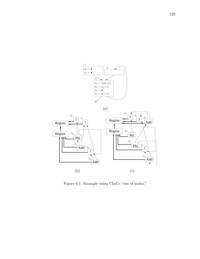
129
t4 ← •
t5 ← t4 + t1
t1 ← •
t0 ← •
1
2
t3 ← t2 + t1
3
t2 ← φ(t0, t5)
(a)
Region
Region
?
Phi
Add
Add
??
t0
t2
t1
t3
t4
t5
Region
Region
?
Phi
Add
??
Add
Phi
t0
t2
t1
t3
t4
t5
t6
(b) (c)
Figure 6.1. Example using Click’s “sea of nodes.”
130
6.1.3 Redundancy percentage
Let us make a few observations on our experimental results. First, our static
numbers tell how many times we have improved at least one path, giving no insight to
how many times the improved paths are used dynamically. Second, the disappointing
performance results suggest that many real programs do not have enough redundancy
to benefit from optimizations like this. We further observe that algorithms like
LEPRE are approximations, and even algorithms like GVNPRE that have a certain
form of theoretical completeness still deal with only static, not dynamic, redundancy.
We propose to study how much run-time redundancy typical applications have, and
how much of that redundancy is removed by our and similar algorithms. This would
require dynamic profiling: how often is a computed value already present in the
registers or memory? Jikes RVM has profiling infrastructure, but it would require
modification to monitor this sort of data. A similar study was done by Bodık et
al [75].
6.1.4 Register pressure
As stated elsewhere, one factor handicapping the effectiveness of PRE is register
pressure. In particular, we have noticed a fair amount of performance degradation on
Pentium, an architecture with comparatively few registers. This situation has been
investigated previously; for example, Simpson’s dissertation contains a chapter on
the relief of register pressure [45]. In that work, Simpson proposed using heuristics
to insert operations after PRE or related optimizations but before register allocation
in hopes that these inserted operations, while introducing new redundancy, will free
more registers. We propose developing heuristic approaches to limit the hoisting of
instructions in the first place. Moreover, our experiments were in a compiler that
uses a fairly simple register allocation [71]. Perhaps we would see more improvement
if conventional, more powerful register allocations were used.

131
6.2 Conclusion
The goal stated in the introduction was to present practical, complete, and effec-
tive algorithms for removing redundancy. Our algorithms ASSAPRE and GVNPRE
have demonstrated themselves to be practical from a software engineering perspec-
tive in that they simplify the task of compiler construction. We claim that LEPRE is
also practical in that it is a fairly straightforward extension to a known approach. A
highlight is the completeness of GVNPRE, in how it subsumes older PRE and GVN
techniques, unifying them in a single analysis. LEPRE is not complete, but provides
experience and intuition for a proposed complete solution. Our experimental results
have shown that there are indeed programs that benefit from these optimizations
and others like them; however, the effect they have varies among benchmarks and
architectures. While the contribution towards effectiveness is only modest, we have
provided compiler construction tools with strong theoretical attributes while raising
a new question: within current trends of software and architecture, how much will
programs benefit by redundancy elimination, no matter how accurate or aggressive?

LIST OF REFERENCES

132
LIST OF REFERENCES
[1] Fred Chow, Sun Chan, Robert Kennedy, Shin-Ming Liu, Raymond Lo, andPeng Tu. A new algorithm for partial redundancy elimination based on SSAform. In Proceedings of the Conference on Programming Language Design andImplementation, pages 273–286, Las Vegas, Nevada, June 1997.
[2] Robert Kennedy, Sun Chan, Shin-Ming Liu, Raymond Lo, Peng Tu, and FredChow. Partial redundancy elimination. ACM Transactions on ProgrammingLanguages and Systems, 21(3):627–676, May 1999.
[3] Stephen Fink, Kathleen Knobe, and Vivek Sarkar. Unified analysis of arrayand object references in strongly typed languages. In Proceedings of the StaticAnalysis Symposium, pages 155–174, Santa Barbara, California, July 2000.
[4] Alfred V. Aho, Ravi Sethi, and Jeffrey D. Ullman. Compilers—Principles,Techniques, and Tools. Addison Wesley, 1986.
[5] Ron Cytron, Jeanne Ferrante, Barry K. Rosen, Mark N. Wegman, and F. Ken-neth Zadeck. Efficiently computing static single assignment form and the controldependence graph. ACM Transactions on Programming Languages and Systems,13(4):451–490, October 1991.
[6] B. K. Rosen, M. N. Wegman, and F. K. Zadeck. Global value numbers andredundant computations. In Proceedings of the 15th Symposium on Principlesof Programming Languages, pages 12–27. ACM Press, 1988.
[7] B. Alpern, C. R. Attanasio, J. J. Barton, M. G. Burke, P.Cheng, J.D. Choi,A. Cocchi, S. J. Fink, D. Grove, M. Hind, S. F. Hummel, D. Lieber, V. Litvinov,M. F. Mergen, T. Ngo, J. R. Russell, V. Sarkar, M. J. Serrano, J. C. Shepherd,S. E. Smith, V. C. Sreedhar, H. Srinivasan, and J. Whaley. The Jalapeno virtualmachine. IBM System Journal, 39(1):211–244, February 2000.
[8] Michael G. Burke, Jong-Deok Choi, Stephen Fink, David Grove, Michael Hind,Vivek Sarkar, M. Serrano, V. Sreedhar, H. Srinvasan, and J. Whaley. TheJalapeno dynamic optimizing compiler for Java. In The Proceedings of the JavaGrande Conference, pages 129–141, San Fransisco, California, June 1999.
[9] IBM Research. The Jikes Research Virtual Machine.http://www-124.ibm.com/developerworks/oss/jikesrvm/.
[10] Bowen Alpern, Mark Wegman, and Kenneth Zadeck. Detecting equality ofvariables in programs. In Proceedings of the Symposium on Principles of Pro-gramming Languages, pages 1–11, San Diego, California, January 1988.
[11] Standard Performance Evalution Corporation. SPECjvm 98 Benchmarks, 1998.http://www.spec.org/osg/jvm98/.

133
[12] Roldan Pozo and Bruce Miller. Scimark 2.0. http://math.nist.gov/scimark2/.
[13] EPCC. The Java Grande Forum Benchmark Suite.http://www.epcc.ed.ac.uk/javagrande/index 1.html.
[14] Architecture and Language Implementation Laboratory. Jolden benchmarksuite. http://www-ali.cs.umass.edu/DaCapo/benchmarks.html. Described in[76].
[15] Thomas VanDrunen and Antony L Hosking. Anticipation-based partial redun-dancy elimination for static single assignment form. Software—Practice & Ex-perience, 34(14), nov 2004. To appear.
[16] Thomas VanDrunen and Antony L Hosking. Value-based partial redundancyelimination. In Proceedings of the International Conference on Compiler Con-struction, Barcelona, Spain, March 2004. LNCS 2985.
[17] Thomas VanDrunen and Antony L Hosking. Corner cases in value-based partialredundancy elimination. Technical Report CSD-TR#03-032, Purdue UniversityDepartment of Computer Sciences, 2003.
[18] John Cocke. Global common subexpression elimination. In Proceedings ofa Symposium on Compiler Optimization, University of Illinois at Urbana-Champaign, 1970.
[19] John Cocke and J. T. Schwartz. Programming Languages and Their Compilers:Preliminary Notes. New York : Courant Institute of Mathematical Sciences,New York University, 1970.
[20] Jeffrey Young. Gary Kildall: The DOS that wasn’t. Forbes, July 1997.
[21] Gary A. Kildall. A code synthesis filter for basic block optimization. Techni-cal Report TR# 72-06-02, University of Washington Computer Science Group,University of Washington, Seatle, Washington, June 1972.
[22] Gary A. Kildall. A unified approach to global program optimization. In Proceed-ings of the Symposium on Principles of Programming Languages, pages 194–206.ACM Press, 1973.
[23] Etienne Morel and Claude Renvoise. A global algorithm for the elimination ofpartial redundancies. In Proceedings of the Second International Symposium onProgramming, pages 147–159, Paris, France, April 1976.
[24] Etienne Morel and Claude Renvoise. Global optimization by supression of par-tial redundancies. Communications of the ACM, 22(2):96–103, 1979.
[25] Karl-Heinz Drechsler and Manfred P. Stadel. A solution to a problem with Moreland Renvoise’s “Global optimization by suppression of partial redundancies”.ACM Transactions on Programming Languages and Systems, 10(4):635–640,October 1988.
[26] Arthur Sorkin. Some comments on “A solution to a problem with Morel andRenvoise’s ‘Global optimization by suppression of partial redundancies’ ”. ACMTransactions on Programming Languages and Systems, 11(4):666–668, 1989.

134
[27] D. M. Dhamdhere. A fast algorithm for code movement optimisation. SIGPLANNotices, 23(10):172–180, 1988.
[28] Dhananjay M. Dhamdhere. Practical adaptation of the global optimization al-gorithm of Morel and Renvoise. ACM Transactions on Programming Languagesand Systems, 13(2):291–294, April 1991.
[29] Jens Knoop, Oliver Ruthing, and Bernhard Steffen. Lazy code motion. In Pro-ceedings of the Conference on Programming Language Design and Implementa-tion, pages 224–234, San Francisco, California, July 1992. SIGPLAN Notices27(7), July 1992.
[30] Jens Knoop, Oliver Ruthing, and Bernhard Steffen. Optimal code motion: The-ory and practice. ACM Transactions on Programming Languages and Systems,16(4):1117–1155, July 1994.
[31] Dhananjay M. Dhamdhere, Barry K. Rosen, and F. Kenneth Zadeck. Howto analyze large programs efficiently and informatively. In Proceedings of theConference on Programming Language Design and Implementation, pages 212–223, 1992.
[32] Karl-Heinz Drechsler and Manfred P. Stadel. A variation of Knoop, Ruthing,and Steffen’s “Lazy code motion”. ACM SIGPLAN Notices, 28(5):29–38, May1993.
[33] Michael Wolfe. Partial redundancy elimination is not bidirectional. SIGPLANNotices, 34(6):43–46, 1999.
[34] Preston Briggs and Keith D. Cooper. Effective partial redundancy elimina-tion. In Proceedings of the Conference on Programming Language Design andImplementation, pages 159–170, Orlando, Florida, June 1994.
[35] Vineeth Kumar Paleri, Y. N. Srikant, and Priti Shankar. A simple algorithmfor partial redundancy elimination. SIGPLAN Notices, 33(12):35–43, 1998.
[36] Oliver Ruthing, Jens Knoop, and Bernhard Steffen. Sparse code motion. InProceedings of the Symposium on Principles of Programming Languages, pages170–183, 2000.
[37] Antony L. Hosking, Nathaniel Nystrom, David Whitlock, Quintin Cutts, andAmer Diwan. Partial redundancy elimination for access path expressions.Software—Practice and Experience, 31(6):577–600, 2001.
[38] Cliff Click and Michael Paleczny. A simple graph-based intermediate represen-tation. In Papers from the Workshop on Intermediate Representations, pages35–49, January 1995.
[39] Andrew W. Appel. Simple generational garbage collection and fast allocation.Software–Practice and Experience, 19(2):171–183, February 1989.
[40] Kathleen Knobe and Vivek Sarkar. Array SSA form and its use in Paral-lelizaiton. In popl, pages 107–120, San Diego, California, January 1998.
[41] Cliff Click and Keith D. Cooper. Combining analyses, combining optimizations.ACM Transactions Programming Languages and Systems, 17(2):181–196, 1995.
135
[42] Cliff Click. Combining Analyses, Combining Optimizations. PhD thesis, RiceUniversity, Houston, Texas, 1995.
[43] Cliff Click. Global code motion, global value numbering. In Proceedings ofthe Conference on Programming Language Design and Implementation, pages246–257, La Jolla, California, June 1995. SIGPLAN Notices 30(6), June 1995.
[44] Preston Briggs, Keith D. Cooper, and L. Taylor Simpson. Value numbering.Software—Practice and Experience, 27(6):701–724, 1997.
[45] Loren Taylor Simpson. Value-driven redundancy elimination. PhD thesis, RiceUniversity, 1996.
[46] Kenneth Cooper and Taylor Simpson. SCC-based value numbering. TechnicalReport CRPC-TR 95636-S, Rice University, Houston, Texas, October 1995.
[47] Steven Muchnick. Advanced Compiler Design and Implementation. MorganKaufmann, 1997.
[48] Bernhard Steffen. Optimal run-time optimization—proved by a new look atabstract interpretation. In Proceedings of the International Joint Conference onTheory and Practice of Software Development, pages 52–68, Pisa, Italy, 1987.LNCS 249.
[49] Bernhard Steffen. Abstrakte Interpretationen beim Optimieren von Pro-grammlaufzeiten. Ein Optimalitatskonzept und seine Anwendung. PhD thesis,Christian-Albrechts-Universitat Kiel, 1987.
[50] Patrick Cousot and Radhia Cousot. Abstract interpretation: a unified lat-tice model for static analysis of program by construction or approximation offixpoints. In Proceedings of the Symposium on Principles of Programming Lan-guages, Los Angeles, California, 1977.
[51] Karthik Gargi. A sparse algorithm for predicated global value numbering. InProceedings of the Conference on Programming Language Design and Imple-mentation, pages 45–56, Berlin, Germany, June 2002.
[52] Oliver Ruthing, Bernhard Steffen, and Jens Knoop. Detecting equalities ofvariables—combining efficiency with precision. In Proceedings of the Static Anal-ysis Symposium, pages 232–247, Venice, Italy, 1999.
[53] Bernhard Steffen, Jens Knoop, and Oliver Ruthing. The value flow graph—aprogram representation for optimal program transformations. In Proceedingsof the European Symposium on Programming (ESOP), pages 389–405, Copen-hagen, Denmark, 1990. LNCS 432.
[54] Bernhard Steffen, Jens Knoop, and Oliver Ruthing. Efficient code motion andan adaptation to strength reduction. In Proceedings of the International JointConference on Theory and Practice of Software Development, Brighton, UnitedKingdom, 1991. LNCS 494.
[55] Jens Knoop, Oliver Ruthing, and Bernhard Steffen. Code motion and codeplacement: Just synonyms? In Proceedings of the European Symposium onProgramming, pages 154–169, Lisbon, Portugal, 1998. LNCS 1381.

136
[56] Jens Knoop, Oliver Ruthing, and Bernhard Steffen. Expansion-based removalof semantic partial redundancies. In Proceedings of the International Conferenceon Compiler Construction, pages 91–106, Amsterdam, The Netherlands, 1999.LNCS 1575.
[57] Rastislav Bodık and Sadun Anik. Path-sensitive value-flow analysis. In Proceed-ings of the Symposium on Principles of Programming Languages, pages 237–251,San Diego, California, January 1998.
[58] Rastislav Bodık, Rajiv Gupta, and Mary Lou Soffa. Complete removal of redun-dant expressions. In Proceedings of the Conference on Programming LanguageDesign and Implementation, pages 1–14, Montreal, Quebec, June 1998.
[59] Rastislav Bodık. Path-Sensitive, Value-Flow Optimizations of Programs. PhDthesis, University of Pittsburgh, 1999.
[60] Rajiv Gupta and Rastislav Bodık. Register pressure sensitive redundancy elim-ination. In International Conference on Compiler Construction, pages 107–121,Amsterdam, Netherlands, March 1999. LNCS 1575.
[61] Dhananjay M. Dhamdhere. E-path pre—partial redundancy elimination madeeasy. ACM SIGPLAN Notices, 37(8):53–65, August 2002.
[62] David Whitlock. The BLOAT book, 1999.Availible at http://www.cs.purdue.edu/vandrutj/bloat.
[63] William Strunk and E. B. White. The Elements of Style. Macmillan, New York,1972.
[64] Andrew W. Appel. Modern Compiler Implementation in Java. CambridgeUniversity Press, Cambridge, UK, 1998. Editions for ML and C also available.
[65] Programming for Persistent Systems Research Group.bytecode level optimization and analysis tool for java.Available for download, http://www.cs.purdue.edu/s3/projects/bloat/, June1999. See programmer’s comment in source code.
[66] William Pugh. Fixing the Java memory model. In The Proceedings of the JavaGrande Conference, pages 89–98, San Fransisco, California, June 1999.
[67] Dan Berlin. Private correspondence, March 2004.
[68] Tim Lindholm and Frank Yellin. The Java Virtual Machine Specification.Addison-Wesley, 1999.
[69] Report 041-R1. Anonymous reviewer’s comments for the program committee,December 2003. The International Conference on Compiler Construction.
[70] The GNU compiler collection project. http://gcc.gnu.org.
[71] Massimiliano Poletto and Vivek Sarkar. Linear scan register allocation. ACMTransactions on Programming Languages and Systems, 21(5):895–913, 1999.
[72] Intel Corporation, P.O. Box 6937, Denver, Colorado. IA-32 Intel ArchitectureSoftware Developer’s Manual, Volume 3: System Programming Guide, 2004.http://www.intel.com/design/pentium4/manuals/253665.htm.
137
[73] Amer Diwan, Kathryn S. McKinley, and J. Eliot B. Moss. Type-based aliasanalysis. ACM SIGPLAN Notices, 33(5):106–117, 1998.
[74] Sun Microsystems. The Java HotSpot Virtual Machine, v 1.4.1, d2 edition,September 2002.
[75] Rastislav Bodık, Rajiv Gupta, and Mary Lou Soffa. Load-reuse analysis: Designand evaluation. In Proceedings of the Conference on Programming LanguageDesign and Implementation, pages 64–76, Atlanta, Georgia, May 1999.
[76] Brendon Cahoon and Katherine McKinley. Data flow analysis for softwareprefetching linked data structures in Java. In Proceedings of the InternationalConference on Parallel Architectures and Compilation Techniques, pages 280–291, Barcelona, Spain, September 2001.

VITA

138
VITA
Thomas VanDrunen grew up in Oak Brook, Illinois, which is famous for being
home to McDonald’s Corporation, being the Polo capital of the world, and be-
ing founded by the father of the producer of the broadway musical Hair. Thomas
attended high school at Timothy Christian High School (Elmhurst, Illinois) and re-
ceived his B.S. from Calvin College (Grand Rapids, Michigan) in 1998, his M.S.
from Purdue University in 2000, and his Ph.D. from Purdue University in 2004. His
computer science interests include compilers, the design and theory of programming
languages, virtual machines, object oriented programming, software engineering, and
computer science instruction. When he’s not doing computer science Thomas enjoys
reading theology, studying ancient Greek, and brewing beer. He is also interested in
Mozart, the history of the Protestant Reformation, musical versifications of the Book
of Psalms, and college football. He has composed a ballad on the life of Benjamin
Franklin.