partialupdateadaptivefiltering...partialupdateadaptivefiltering bei xie abstract adaptive ﬁlters...

Partial Update Adaptive Filtering

Bei Xie

Dissertation submitted to the Faculty of the

Virginia Polytechnic Institute and State University

in partial fulfillment of the requirements for the degree of

Doctor of Philosophy

in

Electrical Engineering

Tamal Bose

William H. Tranter

Aloysius A. Beex

Dong S. Ha

Madhav V. Marathe

December 5, 2011

Blacksburg, Virginia

Keywords: Partial Update, Adaptive Filter, CMA1-2, NCMA, LSCMA, RLS, EDS, CG

Copyright 2011, Bei Xie

Partial Update Adaptive Filtering

Bei Xie

ABSTRACT

Adaptive filters play an important role in the fields related to digital signal processing and

communication, such as system identification, noise cancellation, channel equalization, and

beamforming. In practical applications, the computational complexity of an adaptive filter

is an important consideration. The Least Mean Square (LMS) algorithm is widely used

because of its low computational complexity (O(N)) and simplicity in implementation. The

least squares algorithms, such as Recursive Least Squares (RLS), Conjugate Gradient (CG),

and Euclidean Direction Search (EDS), can converge faster and have lower steady-state mean

square error (MSE) than LMS. However, their high computational complexity (O(N2)) makes

them unsuitable for many real-time applications. A well-known approach to controlling

computational complexity is applying partial update (PU) method to adaptive filters. A

partial update method can reduce the adaptive algorithm complexity by updating part of

the weight vector instead of the entire vector or by updating part of the time. An analysis

for different PU adaptive filter algorithms is necessary and meaningful. The deficient-length

adaptive filter addresses a situation in system identification where the length of the estimated

filter is shorter than the length of the actual unknown system. It is related to the partial

update adaptive filter, but has different performance. It can be viewed as a PU adaptive

filter, in that the deficient-length adaptive filter also updates part of the weight vector.

However, it updates the same part of the weight vector for each iteration, while the partial

update adaptive filter updates a different part of the weight vector for each iteration.

In this work, basic PU methods are applied to the adaptive filter algorithms which have not

been fully addressed in the literature, including CG, EDS, and Constant Modulus Algorithm

(CMA) based algorithms. A new PU method, the selective-sequential method, is developed

for LSCMA. Mathematical analysis is shown including convergence condition, steady-state

performance, and tracking performance. Computer simulation with proper examples is also

shown to further help study the performance. The performance is compared among different

PU methods or among different adaptive filtering algorithms. Computational complexity is

calculated for each PU method and each adaptive filter algorithm. The deficient-length RLS

and EDS are also analyzed and compared to the performance of the PU adaptive filter.

In this dissertation, basic partial-update methods are applied to adaptive filter algorithms

including CMA1-2, NCMA, Least Squares CMA (LSCMA), EDS, and CG. A new PU

method, the selective-sequential method, is developed for LSCMA. Mathematical deriva-

tion and performance analysis are provided including convergence condition, steady-state

mean and mean-square performance for a time-invariant system. The steady-state mean

and mean-square performance are also presented for a time-varying system. Computational

complexity is calculated for each adaptive filter algorithm. Numerical examples are shown

to compare the computational complexity of the PU adaptive filters with the full-update

filters. Computer simulation examples, including system identification and channel equal-

ization, are used to demonstrate the mathematical analysis and show the performance of

PU adaptive filter algorithms. They also show the convergence performance of PU adap-

tive filters. The performance is compared between the original adaptive filter algorithms and

different partial-update methods. The performance is also compared among similar PU least-

squares adaptive filter algorithms, such as PU RLS, PU CG, and PU EDS. Deficient-length

RLS and EDS are studied. The performance of the deficient-length filter is also compared

with the partial update filter. In addition to the generic applications of system identification

and channel equalization, two special applications of using partial update adaptive filters are

also presented. One application is using PU adaptive filters to detect Global System for Mo-

iii

bile Communication (GSM) signals in a local GSM system using the Open Base Transceiver

Station (OpenBTS) and Asterisk Private Branch Exchange (PBX). The other application

is using PU adaptive filters to do image compression in a system combining hyperspectral

image compression and classification.

Overall, the PU adaptive filters can usually achieve comparable performance to the full-

update filters while reducing the computational complexity significantly. The PU adaptive

filters can achieve similar steady-state MSE to the full-update filters. Among different PU

methods, the MMax method has a convergence rate very close to the full-update method.

The sequential and stochastic methods converge slower than the MMax method. However,

the MMax method does not always perform well with the LSCMA algorithm. The sequential

LSCMA has the best performance among the PU LSCMA algorithms. The PU CMA may

perform better than the full-update CMA in tracking a time-varying system. The MMax

EDS can converge faster than the MMax RLS and CG. It can converge to the same steady-

state MSE as the MMax RLS and CG, while having a lower computational complexity. The

PU LMS and PU EDS can also perform a little better in a system combining hyperspectral

image compression and classification.

iv

Acknowledgements

Upon the completion of this dissertation, there are lots of people I would like to thank.

First of all, I am sincerely grateful to my advisor, Dr. Bose, who provided me with a great

opportunity to do research and projects, and gave precious guidance, help, and support to

my research. Additionally, I would like to give special thanks to Dr. Brian Agee, who gave

me a lot of advice and help in the research of CMA. I would like to thank Dr. Tranter, Dr.

Beex, Dr. Ha, and Dr. Marathe, my committee members, for their suggestions and support

in my research. This work was supported in part by NASA AISR grant NNG06GE95G.

Next, I would like to thank Dr. Erzebet Merenyi who helped me in the work of hyperspectral

image compression and classification. My thanks must also go to Dr. Majid Manteghi and

Thomas Tsou, who helped me a lot with the OpenBTS project. I cannot forget the help

of Cyndy Graham, for her kindness and patience, especially for her enormous help in my

written English.

I am grateful too for the support from the precious faculty, staff, and students at the ECE

department. I also need to express my gratitude and deep appreciation to my friends Qian

Liu, Qinqin Chen, Yue Yan, Xuetao Chen, Xu Guo, An He, Zhimin Chen, Xiaoshu Li, Jing

Pan, Meijing Zhang, Sabina Page, Gary Chiu, Frankie Chiu, Siewsun Wong, Jie Lu, Beijie

Xu, Zheng Lu, and Rui Min, for their friendship, hospitality, knowledge, and wisdom that

have supported, enlightened, and helped me over my PhD study and life.

v

Last but not least, I would like to express my love and gratitude to my parents for their

endless love and support in my life.

vi

List of Abbreviations

ADPCM Adaptive differential pulse code modulationANN Artificial neural networkAWGN Additive white Gaussian noiseBER Bit error rateBSC Base station controllerBTS Base transceiver stationCG Conjugate gradientCMA Constant modulus algorithmCMCF Constant modulus cost functionDPCM Differential pulse code modulationEDS Euclidean direction searchFCB Frequency correction burst

vii

FM Frequency modulationFSE Fractionally-spaced equalizeri.i.d. Independent and identically distributedIMSI International mobile subscriber identityISI Inter-symbol interferenceGMSK Gaussian minimum shift keyingGSM Global system for mobile communicationLCVF Lunar Crater Volcanic FieldLMS Least mean squareLSCMA Least squares constant modulus algorithmMS Mobile stationMSC Mobile switch centerMSE Mean-square errorNCMA Normalized constant modulus algorithmOpenBTS Open base transceiver stationPBX Private branch exchangePCS Personal communications servicePSK Phase shift keyingPU Partial updateQAM Quadrature amplitude modulationQPSK Quadrature phase shift keyingRLS Recursive least squaresSDCMA Steepest-descent constant modulus algorithmSER Symbol error rateSIM Subscriber identity moduleSINR Signal to interference plus noise ratioSIP Session initiation protocolSMS Short message serviceSNR Signal to noise ratioSOM Self-organizing mapSWNR Signal to white noise ratioUSRP Universal software radio peripheralVLR Visitor location registerVoIP Voice over IP

viii

Contents

1 Introduction 1

1.1 Motivation . . . . . . . . . . . . . . . . . . . . . . . . . . . . . . . . . . . . . 1

1.2 Problem Statement . . . . . . . . . . . . . . . . . . . . . . . . . . . . . . . . 2

1.3 Organization of the Dissertation . . . . . . . . . . . . . . . . . . . . . . . . . 4

2 Background 6

2.1 Basic Adaptive Filter Models . . . . . . . . . . . . . . . . . . . . . . . . . . 6

2.1.1 System Identification . . . . . . . . . . . . . . . . . . . . . . . . . . . 6

2.1.2 Channel Equalization . . . . . . . . . . . . . . . . . . . . . . . . . . . 8

2.2 Existing Work on Partial Update Adaptive Filters . . . . . . . . . . . . . . . 10

2.3 Partial Update Methods . . . . . . . . . . . . . . . . . . . . . . . . . . . . . 11

2.3.1 Periodic Partial Update Method . . . . . . . . . . . . . . . . . . . . . 12

2.3.2 Sequential Partial Update Method . . . . . . . . . . . . . . . . . . . 13

2.3.3 Stochastic Partial Update Method . . . . . . . . . . . . . . . . . . . . 14

ix

2.3.4 MMax Method . . . . . . . . . . . . . . . . . . . . . . . . . . . . . . 14

3 Partial Update CMA-based Algorithms for Adaptive Filtering 15

3.1 Motivation . . . . . . . . . . . . . . . . . . . . . . . . . . . . . . . . . . . . . 15

3.2 Review of Constant Modulus Algorithms . . . . . . . . . . . . . . . . . . . . 16

3.3 Partial Update Constant Modulus Algorithms . . . . . . . . . . . . . . . . . 19

3.3.1 Partial Update CMA . . . . . . . . . . . . . . . . . . . . . . . . . . . 19

3.3.2 Partial Update NCMA . . . . . . . . . . . . . . . . . . . . . . . . . . 20

3.3.3 Partial Update LSCMA . . . . . . . . . . . . . . . . . . . . . . . . . 20

3.4 Algorithm Analysis for a Time-Invariant System . . . . . . . . . . . . . . . . 22

3.4.1 Steady-State Performance of Partial Update SDCMA . . . . . . . . . 22

3.4.2 Steady-State Performance of Partial Update Dynamic LSCMA . . . . 27

3.4.3 Convergence Analysis of the PU Static LSCMA . . . . . . . . . . . . 30

3.4.4 Complexity of the PU SDCMA and LSCMA . . . . . . . . . . . . . . 33

3.5 Simulation I – Simple FIR channel . . . . . . . . . . . . . . . . . . . . . . . 36

3.5.1 Convergence Performance . . . . . . . . . . . . . . . . . . . . . . . . 38

3.5.2 Steady-state Performance . . . . . . . . . . . . . . . . . . . . . . . . 41

3.5.3 Complexity . . . . . . . . . . . . . . . . . . . . . . . . . . . . . . . . 44

3.6 Simulation II – LSCMA Performance using a Realistic DSSS System and a

Fractionally-Spaced Equalizer . . . . . . . . . . . . . . . . . . . . . . . . . . 47

3.6.1 Steady-State Performance . . . . . . . . . . . . . . . . . . . . . . . . 52

x

3.6.2 Convergence Performance . . . . . . . . . . . . . . . . . . . . . . . . 53

3.6.3 Complexity and Simulation Time . . . . . . . . . . . . . . . . . . . . 64

3.7 Algorithm Analysis for a Time-Varying System . . . . . . . . . . . . . . . . 68

3.7.1 Algorithm Analysis of CMA1-2 and NCMA for a Time-Varying System 69

3.7.2 Algorithm Analysis of LSCMA for a Time-Varying System . . . . . . 70

3.7.3 Simulation . . . . . . . . . . . . . . . . . . . . . . . . . . . . . . . . . 71

3.8 Conclusion . . . . . . . . . . . . . . . . . . . . . . . . . . . . . . . . . . . . . 79

4 Partial Update CG Algorithms for Adaptive Filtering 83

4.1 Review of Conjugate Gradient Algorithm . . . . . . . . . . . . . . . . . . . . 84

4.2 Partial Update CG . . . . . . . . . . . . . . . . . . . . . . . . . . . . . . . . 86

4.3 Steady-State Performance of Partial Update CG for a Time-Invariant System 88

4.4 Steady-State Performance of Partial Update CG for a Time-Varying System 92

4.5 Simulations . . . . . . . . . . . . . . . . . . . . . . . . . . . . . . . . . . . . 95

4.5.1 Performance of Different PU CG Algorithms . . . . . . . . . . . . . . 95

4.5.2 Tracking Performance of the PU CG using the First-Order Markov

Model . . . . . . . . . . . . . . . . . . . . . . . . . . . . . . . . . . . 103

4.6 Conclusion . . . . . . . . . . . . . . . . . . . . . . . . . . . . . . . . . . . . . 109

5 Partial Update EDS Algorithms for Adaptive Filtering 110

5.1 Motivation . . . . . . . . . . . . . . . . . . . . . . . . . . . . . . . . . . . . . 110

xi

5.2 Review of Euclidean Direction Search Algorithm . . . . . . . . . . . . . . . . 111

5.3 Partial update EDS . . . . . . . . . . . . . . . . . . . . . . . . . . . . . . . . 112

5.4 Performance of Partial Update EDS for a time-invariant system . . . . . . . 114

5.5 Performance of Partial Update EDS for a time-varying system . . . . . . . . 118

5.6 Simulations . . . . . . . . . . . . . . . . . . . . . . . . . . . . . . . . . . . . 120

5.6.1 Performance of PU EDS for a Time-Invariant System . . . . . . . . . 120

5.6.2 Tracking Performance of the PU EDS using the First-Order Markov

Model . . . . . . . . . . . . . . . . . . . . . . . . . . . . . . . . . . . 126

5.7 Conclusion . . . . . . . . . . . . . . . . . . . . . . . . . . . . . . . . . . . . . 131

6 Deficient-Length RLS and EDS 134

6.1 Performance Analysis of Deficient-Length RLS . . . . . . . . . . . . . . . . . 135

6.1.1 Mean Performance . . . . . . . . . . . . . . . . . . . . . . . . . . . . 136

6.1.2 Mean-Square Performance . . . . . . . . . . . . . . . . . . . . . . . . 138

6.1.3 Mean and Mean-Square Performance for Ergodic Input Signal . . . . 141

6.2 Performance Analysis of Deficient-Length EDS . . . . . . . . . . . . . . . . . 144

6.2.1 Mean Performance . . . . . . . . . . . . . . . . . . . . . . . . . . . . 146

6.2.2 Mean-Square Performance . . . . . . . . . . . . . . . . . . . . . . . . 147

6.3 Simulations . . . . . . . . . . . . . . . . . . . . . . . . . . . . . . . . . . . . 148

6.3.1 System Model . . . . . . . . . . . . . . . . . . . . . . . . . . . . . . . 148

6.3.2 Correlated Input . . . . . . . . . . . . . . . . . . . . . . . . . . . . . 149

xii

6.3.3 White Input . . . . . . . . . . . . . . . . . . . . . . . . . . . . . . . . 153

6.3.4 Channel Equalization . . . . . . . . . . . . . . . . . . . . . . . . . . . 153

6.4 Conclusion . . . . . . . . . . . . . . . . . . . . . . . . . . . . . . . . . . . . . 156

7 Special Applications of Partial-Update Adaptive Filters 159

7.1 PU Adaptive Filters in Detecting GSM signals in a local GSM system using

OpenBTS and Asterisk PBX . . . . . . . . . . . . . . . . . . . . . . . . . . . 159

7.2 PU Adaptive Filters in a System Combining Hyperspectral Image Compres-

sion and Classification . . . . . . . . . . . . . . . . . . . . . . . . . . . . . . 164

7.2.1 Simulations . . . . . . . . . . . . . . . . . . . . . . . . . . . . . . . . 170

8 Conclusion 176

8.1 Dissertation Summary . . . . . . . . . . . . . . . . . . . . . . . . . . . . . . 176

8.2 Future Work . . . . . . . . . . . . . . . . . . . . . . . . . . . . . . . . . . . . 178

xiii

List of Figures

2.1 System identification model. . . . . . . . . . . . . . . . . . . . . . . . . . . . 7

2.2 System model. . . . . . . . . . . . . . . . . . . . . . . . . . . . . . . . . . . . 8

2.3 FIR channel and equalizer. . . . . . . . . . . . . . . . . . . . . . . . . . . . . 9

3.1 The number of multiplications vs PU length. . . . . . . . . . . . . . . . . . . 35

3.2 The number of additions vs PU length. . . . . . . . . . . . . . . . . . . . . . 36

3.3 The number of cycles vs PU length. . . . . . . . . . . . . . . . . . . . . . . . 37

3.4 Channel equalization model. . . . . . . . . . . . . . . . . . . . . . . . . . . . 38

3.5 The convergence performance among PU CMA algorithms, PU length=4. . . 39

3.6 Comparison of BER between PU CMA1-2 algorithms and the full-length

CMA1-2, PU length=8. . . . . . . . . . . . . . . . . . . . . . . . . . . . . . . 43

3.7 Comparison of BER between PU CMA1-2 algorithms and the full-length

CMA1-2, PU length=4. . . . . . . . . . . . . . . . . . . . . . . . . . . . . . . 43

3.8 Comparison of BER between PU NCMA algorithms and the full-length NCMA,

PU length=8. . . . . . . . . . . . . . . . . . . . . . . . . . . . . . . . . . . . 44

xiv

3.9 Comparison of BER between PU NCMA algorithms and the full-length NCMA,

PU length=4. . . . . . . . . . . . . . . . . . . . . . . . . . . . . . . . . . . . 45

3.10 Comparison of BER between PU LSCMA algorithms and the full-length

LSCMA, PU length=8. . . . . . . . . . . . . . . . . . . . . . . . . . . . . . . 45

3.11 Comparison of BER between PU LSCMA algorithms and the full-length

LSCMA, PU length=4. . . . . . . . . . . . . . . . . . . . . . . . . . . . . . . 46

3.12 System model. . . . . . . . . . . . . . . . . . . . . . . . . . . . . . . . . . . . 48

3.13 Channel model. . . . . . . . . . . . . . . . . . . . . . . . . . . . . . . . . . . 48

3.14 FSE model. . . . . . . . . . . . . . . . . . . . . . . . . . . . . . . . . . . . . 48

3.15 The spectral response at ADC output. . . . . . . . . . . . . . . . . . . . . . 51

3.16 The CMCF performance of the sequential dynamic LSCMA. . . . . . . . . . 54

3.17 The CMCF performance of the stochastic dynamic LSCMA. . . . . . . . . . 54

3.18 The CMCF performance of the selective-sequential dynamic LSCMA. . . . . 55

3.19 The histogram plot of the number of updates versus weight position, PU

dynamic LSCMA, PU length=16. . . . . . . . . . . . . . . . . . . . . . . . . 55

3.20 The SINR performance of the sequential dynamic LSCMA. . . . . . . . . . . 57

3.21 The SINR performance of the stochastic dynamic LSCMA. . . . . . . . . . . 57

3.22 The SINR performance of the selective-sequential dynamic LSCMA. . . . . . 58

3.23 The SINR performance of the sequential dynamic LSCMA using the a poste-

riori output. . . . . . . . . . . . . . . . . . . . . . . . . . . . . . . . . . . . . 59

xv

3.24 The SINR performance of the stochastic dynamic LSCMA using the a poste-

riori output. . . . . . . . . . . . . . . . . . . . . . . . . . . . . . . . . . . . . 59

3.25 The SINR performance of the selective-sequential dynamic LSCMA using the

a posteriori output. . . . . . . . . . . . . . . . . . . . . . . . . . . . . . . . . 60

3.26 The confidence of the average target BER capture time for LSCMA. . . . . . 62

3.27 The confidence of the average target BER capture time for sequential LSCMA. 62

3.28 The confidence of the average target BER capture time for stochastic LSCMA. 63

3.29 The confidence of the average target BER capture time for selective-sequential

LSCMA. . . . . . . . . . . . . . . . . . . . . . . . . . . . . . . . . . . . . . . 63

3.30 The SINR performance for static LSCMA and PU static LSCMA, PU length=20. 64

3.31 The SINR performance for static LSCMA and PU static LSCMA using the a

posteriori output, PU length=20. . . . . . . . . . . . . . . . . . . . . . . . . 65

3.32 The CMCF performance for PU CMA1-2 for a time-varying system, PU

length=8, ση = 0.001. . . . . . . . . . . . . . . . . . . . . . . . . . . . . . . . 72


length=4, ση = 0.001. . . . . . . . . . . . . . . . . . . . . . . . . . . . . . . . 73


length=8, ση = 0.0001. . . . . . . . . . . . . . . . . . . . . . . . . . . . . . . 73


length=4, ση = 0.0001. . . . . . . . . . . . . . . . . . . . . . . . . . . . . . . 74

3.36 The CMCF performance for PU NCMA for a time-varying system, PU length=8,

ση = 0.001. . . . . . . . . . . . . . . . . . . . . . . . . . . . . . . . . . . . . 75

xvi


ση = 0.001. . . . . . . . . . . . . . . . . . . . . . . . . . . . . . . . . . . . . 75


ση = 0.0001. . . . . . . . . . . . . . . . . . . . . . . . . . . . . . . . . . . . . 76


ση = 0.0001. . . . . . . . . . . . . . . . . . . . . . . . . . . . . . . . . . . . . 76

3.40 The CMCF performance for PU dynamic LSCMA for a time-varying system,

PU length=8, ση = 0.001. . . . . . . . . . . . . . . . . . . . . . . . . . . . . 77


PU length=4, ση = 0.001. . . . . . . . . . . . . . . . . . . . . . . . . . . . . 78


PU length=8, ση = 0.0001. . . . . . . . . . . . . . . . . . . . . . . . . . . . . 78


PU length=4, ση = 0.0001. . . . . . . . . . . . . . . . . . . . . . . . . . . . . 79

4.1 Comparison of MSE of the PU CG with correlated input, M=8. . . . . . . . 96

4.2 Comparison of MSE of the PU CG with correlated input, M=4. . . . . . . . 97

4.3 Comparison of MSE of the PU CG with white input, M=8. . . . . . . . . . . 97

4.4 Comparison of MSE of the PU CG with white input, M=4. . . . . . . . . . . 98

4.5 The mean convergence of the weights at steady state for MMax CG. . . . . . 98

4.6 Comparison of MSE of the PU CG with the PU RLS. . . . . . . . . . . . . . 101

4.7 Decision-directed equalizer diagram. . . . . . . . . . . . . . . . . . . . . . . . 101

xvii

4.8 The frequency response of the channel. . . . . . . . . . . . . . . . . . . . . . 102

4.9 Comparison of SER of the PU CG with the PU RLS. . . . . . . . . . . . . . 103

4.10 Comparison of MSE of the PU CG with CG for white input, N=16, M=8,

and ση = 0.001. . . . . . . . . . . . . . . . . . . . . . . . . . . . . . . . . . . 104


and ση = 0.01. . . . . . . . . . . . . . . . . . . . . . . . . . . . . . . . . . . . 105


and ση = 0.001. . . . . . . . . . . . . . . . . . . . . . . . . . . . . . . . . . . 105


and ση = 0.01. . . . . . . . . . . . . . . . . . . . . . . . . . . . . . . . . . . . 106

4.14 Comparison of MSE of the MMax CG with CG, RLS, and MMax RLS for

white input, N=16, M=8. . . . . . . . . . . . . . . . . . . . . . . . . . . . . 108

4.15 Comparison of MSE of the MMax CG with CG, RLS, and MMax RLS for

white input, N=16, M=4. . . . . . . . . . . . . . . . . . . . . . . . . . . . . 109

5.1 Comparison of MSE of the PU EDS with white input, M=8. . . . . . . . . . 122

5.2 Comparison of MSE of the PU EDS with white input, M=4. . . . . . . . . . 122

5.3 Comparison of MSE of the PU EDS with correlated input, M=8. . . . . . . . 123

5.4 Comparison of MSE of the PU EDS with correlated input, M=4. . . . . . . . 123

5.5 Comparison of MSE of the PU EDS with PU CG and the PU RLS. . . . . . 125

5.6 Comparison of SER of the PU CG with the PU RLS. . . . . . . . . . . . . . 126

xviii

5.7 Comparison of MSE of the PU EDS with the EDS for white input, N=16,

M=8, ση = 0.001. . . . . . . . . . . . . . . . . . . . . . . . . . . . . . . . . . 127


M=8, ση = 0.01. . . . . . . . . . . . . . . . . . . . . . . . . . . . . . . . . . . 128


M=4, ση = 0.001. . . . . . . . . . . . . . . . . . . . . . . . . . . . . . . . . . 128


M=4, ση = 0.01. . . . . . . . . . . . . . . . . . . . . . . . . . . . . . . . . . . 129

5.11 Comparison of MSE of the MMax EDS with the EDS, RLS, MMax RLS, CG,

and MMax CG for white input, N=16, M=8. . . . . . . . . . . . . . . . . . . 131

5.12 Comparison of MSE of the MMax EDS with the EDS, RLS, MMax RLS, CG,

and MMax CG for white input, N=16, M=4. . . . . . . . . . . . . . . . . . . 132

6.1 Comparison of theoretical and simulation curves of the mean behavior of the

6th and 8th coefficient errors of the deficient-length RLS for correlated input,

and N=16, M=12, λ = 0.99, δ−1 = 0.1. . . . . . . . . . . . . . . . . . . . . . 150


6th and 8th coefficient errors of the deficient-length RLS for correlated input,

and N=16, M=12, λ = 0.99, δ−1 = 100. . . . . . . . . . . . . . . . . . . . . . 150

6.3 Comparison of theoretical and simulation curves of the mean-square behavior

of the deficient-length RLS for correlated input, and N=16, M=12, λ = 0.99,

δ−1 = 0.1. . . . . . . . . . . . . . . . . . . . . . . . . . . . . . . . . . . . . . 151

xix


of the deficient-length RLS for correlated input, and N=16, M=12, λ = 0.99,

δ−1 = 100. . . . . . . . . . . . . . . . . . . . . . . . . . . . . . . . . . . . . . 151


6th and 8th coefficient errors of the deficient-length EDS for correlated input,

and N=16, M=12, λ = 0.99. . . . . . . . . . . . . . . . . . . . . . . . . . . . 152


of the deficient-length EDS for correlated input, and N=16, M=12, λ = 0.99. 152


6th and 8th coefficient errors of the deficient-length RLS for white input, and

N=16, M=12, λ = 0.99, δ−1 = 0.1. . . . . . . . . . . . . . . . . . . . . . . . . 153


of the deficient-length RLS for white input, and N=16, M=12, λ = 0.99,

δ−1 = 0.1. . . . . . . . . . . . . . . . . . . . . . . . . . . . . . . . . . . . . . 154


6th and 8th coefficient errors of the deficient-length EDS for white input, and

N=16, M=12, λ = 0.99. . . . . . . . . . . . . . . . . . . . . . . . . . . . . . 154


of the deficient-length EDS for white input, and N=16, M=12,λ = 0.99. . . . 155

6.11 Comparison of SER between RLS and deficient-length RLS. . . . . . . . . . 156

6.12 Comparison of SER between EDS and deficient-length EDS. . . . . . . . . . 157

6.13 The frequency magnitude (left) and impulse (right) responses of the channel. 157

xx

6.14 The frequency magnitude responses of the RLS equalizer (left) and of the

convolution of the channel and the equalizer (right). . . . . . . . . . . . . . . 158

6.15 The frequency magnitude responses of the deficient-length RLS equalizer (left)

and of the convolution of the channel and the equalizer (right). . . . . . . . . 158

7.1 Traditional GSM network. . . . . . . . . . . . . . . . . . . . . . . . . . . . . 160

7.2 GSM network using OpenBTS and Asterisk PBX. . . . . . . . . . . . . . . . 162

7.3 Functional-block description of local GSM system. . . . . . . . . . . . . . . . 163

7.4 Diagram of adaptive line enhancer. . . . . . . . . . . . . . . . . . . . . . . . 164

7.5 A typical hyperspectral image. . . . . . . . . . . . . . . . . . . . . . . . . . . 166

7.6 System combining compression and classification. . . . . . . . . . . . . . . . 168

7.7 One image band of the LCVF scene, obtained at 1.02987 µm. . . . . . . . . 170

7.8 Hyperspectral image of the LCVF scene. . . . . . . . . . . . . . . . . . . . . 171

xxi

List of Tables

3.1 Adaptive Algorithm Complexity . . . . . . . . . . . . . . . . . . . . . . . . . 34

3.2 Overall Complexity . . . . . . . . . . . . . . . . . . . . . . . . . . . . . . . . 36

3.3 The Parameters of Filter Algorithms . . . . . . . . . . . . . . . . . . . . . . 37

3.4 Approximate Convergence Times . . . . . . . . . . . . . . . . . . . . . . . . 40

3.5 Steady-State MSE Comparison among Different PU CMA algorithms . . . . 42

3.6 Adaptive Algorithm Complexity . . . . . . . . . . . . . . . . . . . . . . . . . 46

3.7 Average Target BER Capture Time of PU dynamic LSCMA . . . . . . . . . 61

3.8 Complexity over average target BER capture time using a priori output . . . 66

3.9 Complexity over target BER capture time using a posteriori output . . . . . 67

3.10 Overall simulation time for dynamic LSCMA . . . . . . . . . . . . . . . . . . 68

3.11 Steady-State MSE Comparison among Different PU CMA algorithms for a

time-varying system, ση = 0.001 . . . . . . . . . . . . . . . . . . . . . . . . . 80

3.12 Steady-State MSE Comparison among Different PU CMA algorithms for a

time-varying system, ση = 0.0001 . . . . . . . . . . . . . . . . . . . . . . . . 81

xxii

4.1 The computational complexities of PU CG for real signals. . . . . . . . . . . 87

4.2 The computational complexities of PU CG for complex signals. . . . . . . . . 87

4.3 The simulated MSE and theoretical MSE of PU CG algorithms for correlated

input. . . . . . . . . . . . . . . . . . . . . . . . . . . . . . . . . . . . . . . . 99

4.4 The simulated MSE and theoretical MSE of PU CG algorithms for white input. 99

4.5 The simulated MSE and theoretical MSE of the PU CG in a time-varying

system for white input and process noise ση = 0.001. . . . . . . . . . . . . . 106

4.6 The simulated MSE and theoretical MSE of the PU CG in a time-varying

system for white input and process noise ση = 0.01. . . . . . . . . . . . . . . 107

4.7 The computational complexities of CG, MMax CG, RLS, and MMax RLS. . 108

5.1 The computational complexities of the PU EDS for real signals. . . . . . . . 113

5.2 The computational complexities of the PU EDS for complex signals. . . . . . 113

5.3 The simulated MSE and theoretical MSE of the PU EDS for a time-invariant

system and white input. . . . . . . . . . . . . . . . . . . . . . . . . . . . . . 124

5.4 The simulated MSE and theoretical MSE of the PU EDS for a time-invariant

system and correlated input. . . . . . . . . . . . . . . . . . . . . . . . . . . . 124

5.5 The simulated MSE and theoretical MSE of the PU EDS in a time-varying

system for white input and process noise ση = 0.001. . . . . . . . . . . . . . 129

5.6 The simulated MSE and theoretical MSE of the PU EDS in a time-varying

system for white input and process noise ση = 0.01. . . . . . . . . . . . . . . 130

xxiii

5.7 The computational complexities of the EDS, MMax EDS, RLS, MMax RLS,

CG, and MMax CG. . . . . . . . . . . . . . . . . . . . . . . . . . . . . . . . 132

7.1 The computational complexities of the LMS, periodic LMS, sequential LMS,

EDS, periodic EDS, and sequential EDS . . . . . . . . . . . . . . . . . . . . 164

7.2 Execution time using C and Linux . . . . . . . . . . . . . . . . . . . . . . . . 165

7.3 The comparison of classification accuracies among different predictor algorithms172

7.4 The classification error, in units of (% misclassified samples)/100, of each class

by using different predictor algorithms . . . . . . . . . . . . . . . . . . . . . 175

xxiv

Chapter 1

Introduction

1.1 Motivation

Adaptive filters play an important role in the fields related to digital signal processing and

communication, such as system identification, noise cancellation, channel equalization, and

beamforming. In practical applications, the computational complexity of an adaptive filter

is an important consideration. The Least Mean Square (LMS) algorithm is widely used

[21] because of its low computational complexity (O(N)) and simplicity in implementation.

However, it is well known that the LMS has low convergence speed, especially for correlated

input signals. The least squares algorithms, such as Recursive Least Squares (RLS), Con-

jugate Gradient (CG), and Euclidean Direction Search (EDS), can converge fast and have

low steady-state mean square error (MSE). However, with high computational complexity

(O(N2)), these algorithms need expensive real-time resources, i.e., clock cycles, memory,

and power in a digital signal processor (DSP) or field-programmable gate array (FPGA).

A well-known approach to controlling computational complexity is applying partial update

(PU) method to adaptive filters. A partial update adaptive filter reduces computational

1

2

complexity by updating part of the coefficient vector instead of updating the entire vector

or by updating part of the time. Moreover, the partial update adaptive filters may converge

faster than the full-update filters and achieve lower steady-state MSE in particular applica-

tions [11]. In the literature, partial update methods have been applied to several adaptive

filters, such as LMS, NLMS, RLS, Affine Projection (AP), Normalized Constant Modulus

Algorithm (NCMA), etc. However, there are only a few analyses of these partial update

adaptive filter algorithms. Most analyses are based on partial update LMS and its variants.

Only a few papers have addressed partial update RLS and AP.

1.2 Problem Statement

In this dissertation, the basic partial-update methods are applied to the adaptive filters which

have high computational complexity. We have chosen two least-squares (LS) algorithms,

CG and EDS. Both of these can converge fast and achieve small steady-state MSE. The

complexity is less than the RLS algorithm, but is still O(N2). The PU methods are also

applied to the CMA1-2, NCMA, and Least squares CMA (LSCMA). The LSCMA converges

much faster than the CMA1-2 and NCMA, and it does not have a stability problem. The

computational complexity O(N2) per sample has limited the LSCMA to applications with a

small number of adapted elements such as adaptive arrays and polarization combiners. The

PU LSCMA can reduce the computational complexity and extend the LSCMA in applications

with long filters and fractionally-spaced equalizers (FSE’s). The PU LSCMA is compared

with the steepest-decent CMA (SDCMA) including CMA1-2 and NCMA.

Mathematical analysis has been done for the new partial-update adaptive filter algorithms.

Mathematical analysis has also been extended to the existing PU adaptive filter algorithms.

This work has analyzed the convergence conditions, steady-state performance, and tracking

3

performance. A new PU method, the selective-sequential method, is developed for LSCMA.

The theoretical performance is validated by computer simulations. The performance is com-

pared between the original adaptive filter algorithms and different partial-update methods.

Since a specific PU method in one adaptive filter algorithm which achieves good perfor-

mance may not perform well in another adaptive filter algorithm, the performance of one

PU method for different adaptive filter algorithms is also compared. Computational com-

plexity is calculated for each partial-update method and each adaptive filter algorithm.

Moreover, the adaptive filter performance has been studied in a deficient-length (under-

modeled) case. The deficient-length case exists in the system identification model. In real

world situations, the length of the system model in system identification is not known.

Usually a deficient-length filter will be used to estimate the unknown system. Therefore,

extra error will be caused by the deficient length. Although the concept of the deficient-

length filter is different from the partial update method, the analysis of the deficient-length

filter can be related to the partial update adaptive filter algorithm. In this work, two adaptive

filter algorithms, RLS and EDS, have been studied for the deficient-length performance.

The major contributions of this work are summarized as follows.

1. Basic partial-update methods are applied to adaptive filter algorithms including CMA1-

2, NCMA, Least Squares CMA(LSCMA), EDS, and CG. A new PU method, the

selective-sequential method, is developed for LSCMA.

2. Mathematical derivation and performance analysis are provided including convergence

conditions, steady-state mean and mean-square performance for a time-invariant sys-

tem. The steady-state mean and mean-square performance is also presented for a

time-varying system.

3. Computational complexity is calculated for each adaptive filter algorithm. It is also

4

compared for each partial-update method. Numerical examples are presented to show

how many multiplications or additions can be saved by using a PU adaptive filter.

4. Proper computer simulations demonstrate the mathematical analysis and show the

performance of PU adaptive filter algorithms. The applications include system identi-

fication and channel equalization. The computer simulations also show the convergence

performance of PU adaptive filters. The performance is compared between the origi-

nal adaptive filter algorithms and different partial-update methods. The PU adaptive

filters usually can achieve comparable performance to the full-update filters while re-

ducing the computational complexity significantly.

5. Deficient-length RLS and EDS are studied. The performance of the deficient-length

filter is also compared with the partial update filter.

6. Besides applications of system identification and channel equalization, two special ap-

plications of using partial update adaptive filters are also presented. One application is

using PU adaptive filters to detect Global System for Mobile Communication (GSM)

signals in a local GSM system using OpenBTS and Asterisk PBX. The other appli-

cation is using PU adaptive filters to do image compression in a system combining

hyperspectral image compression and classification.

1.3 Organization of the Dissertation

This dissertation is organized as follows. Chapter 2 (Background) introduces basic adaptive

signal processing models, partial update methods, and a literature review on existing partial-

update adaptive filter algorithms. Chapter 3 shows the performance of partial-update CMA-

based algorithms, including CMA1-2, NCMA, and LSCMA. Chapters 4, and 5 show the

5

performance of the partial-update CG and partial-update EDS algorithms, respectively. The

comparison among PU RLS, CG, and EDS is shown. Chapter 6 shows the performance

of deficient-length RLS and EDS. The performance is compared with PU RLS and EDS.

Chapter 7 shows the special applications of partial-update adaptive filters.

Chapter 2

Background

In Section 2.1, basic adaptive signal processing models are introduced. Section 2.2 reviews

the existing partial-update adaptive filter algorithms. The basic partial update methods

considered in this work are introduced and defined in Section 2.3.

2.1 Basic Adaptive Filter Models

Adaptive filters have been used in many applications, such as in system identification, noise

cancellation, echo cancellation, channel equalization, signal prediction, and beamforming. In

this section, models of system identification and channel equalization will be described in

detail because they will be used as applications in Chapters 3 to 5.

2.1.1 System Identification

System identification is used to estimate an unknown linear or nonlinear system in digital

signal processing. A block diagram for system identification is given in Fig. 2.1. An input is

6

7

Figure 2.1: System identification model.

applied to the unknown system and the adaptive filter simultaneously. Usually a noise will

be added at the output of the unknown system. If the unknown system does not change

with time, then it is a time-invariant system. If the unknown system changes with time,

then it is a time-varying system.

The system identification model can be presented as:

d(n) = xT (n)wo + v(n), (2.1)

where d(n) is the desired signal, x(n) = [x(n), x(n− 1), ..., x(n−N + 1)]T is the input data

vector of the unknown system, wo(n) = [wo1, w

o2, ..., w

oN ]

T is the impulse response vector of

the unknown system, and v(n) is zero-mean white noise, which is independent of any other

signals.

Let w be the coefficient vector of an adaptive filter. The estimated signal y(n) is defined as

y(n) = xT (n)w(n), (2.2)

8

Figure 2.2: System model.

and the output signal error is defined as

e(n) = d(n)− xT (n)w(n). (2.3)

The error will be fed back to update the adaptive filter.

2.1.2 Channel Equalization

In a typical wireless communication system, the transmitted signal is subjected to noise

and multipath which causes delay, distortion, and inter-symbol-interference (ISI). A channel

equalizer is generally used to remove the multipath channel effects. A typical wireless com-

munication system is shown in Fig. 2.2. The channel and equalizer shown in Fig. 2.2 can

be modelled as FIR filters, which are shown in Fig. 2.3.

9

Figure 2.3: FIR channel and equalizer.

Using the transmission channel shown in Fig. 2.3, the received signal x(n) is modeled by

x(n) = ε(n) +L−1∑

ℓ=0

cℓs(n− ℓ)

= ε(n) + sT (n)c, (2.4)

where c = [ c0 · · · cL−1 ]T is the L × 1 vector representation of the FIR channel impulse

response, s(n) = [ s(n) · · · s(n− L+ 1) ]T is the L × 1 transmitted signal state vector,

and ε(n) is the background noise and interference added to the desired signal at the receiver,

and where (·)T denotes the matrix transpose operation. Similarly, the recovered (equalizer

output) signal is given by

y(n) =N−1∑

i=0

wix(n− i)

= xT (n)w, (2.5)

10

wherew = [ w0 · · · wN−1 ]T is theN×1 vector representation of the FIR equalizer impulse

response (referred to here as the equalizer weight vector), and where

x(n) = [ x(n) · · · x(n−N + 1) ]T , (2.6)

is the N × 1 received signal state vector. The goal of the equalizer adaptation algorithm is

to design an equalizer weight vector that can remove the channel distortion from the desired

signal, such that the convolved channelizer and equalizer impulse response∑

cmwn−m ≈ δq

for some group delay q, without unduly raising the signal-to-noise ratio (SNR) of the equalizer

output signal. In conventional nonblind systems, this is typically accomplished by adapting

the equalizer to minimize the mean-square error (MSE) between the equalizer output signal

y(n) and the transmitted signal s(n) over some known component of s(n), e.g., some known

training or pilot sequence transmitted as part of s(n). For a blind equalizer, a training

sequence is not used.

2.2 Existing Work on Partial Update Adaptive Filters

The partial-update (PU) method is a straightforward approach to controlling the computa-

tional complexity because it only updates part of the coefficient vector instead of updating

the entire filter vector. In the literature, partial update methods have been mostly studied

for LMS and its variants [12], [13], [19], [34], [29], [54], [11]. Partial update methods such

as periodic PU, sequential PU, stochastic PU, MMax update method, selective PU method,

set membership PU method, and the block PU method have been applied to LMS or NLMS.

The stability condition, robustness, mean convergence analysis, mean-square convergence

analysis, and tracking performance have been done for LMS or NLMS. Moreover, the PU

11

LMS for sparse impulse responses [8], [30] and PU Transform-Domain LMS [1], [2] have

been addressed. In [14, 40, 45, 46], new PU methods as such proportionate normalized least-

mean-squares (PNLMS), improved PNLMS (IPNLMS), select and queue with a constraint

(SELQUE) method, and modified SELQUE (M-SELQUE) method are also developed for

sparse impulse responses and aim to improve the convergence rate of NLMS in echo can-

cellation systems. In [38], the MMax RLS and MMax AP have been analyzed for white

inputs. In [29], the tracking performance has been analyzed for MMax RLS and MMax AP.

In [6], an analysis of the transient and the steady-state behavior of a filtered-x partial-error

affine projection algorithm was provided. In [53], [9], set-membership AP was proposed, but

the mathematic analysis was not provided. In [10], [11], the selective PU NCMA has been

proposed. However, the mathematic analysis was not provided.

2.3 Partial Update Methods

Instead of updating all of the N × 1 coefficients, the partial-update method only updates

M×1 coefficients, where M < N . In this work, we consider the basic partial update methods

including periodic PU [13], sequential PU [13], stochastic PU [19], and MMax update method

[12]. The set-membership PU method is not considered here because it was developed for

steepest-decent methods such as LMS and AP. It aims to adjust a time-variant step-size for

these algorithms. A detailed description of periodic, sequential, stochastic, and MMax PU

methods will be given in this section.

The weight-update function of a typical adaptive filter can be written as

w(n+ 1) = w(n) +∆w(n). (2.7)

12

The partial-update method chooses M elements from the ∆w and generates the new weights.

It modifies (2.7) to

wi(n+ 1) =

wi(n) + ∆wi(n) if i ∈ IM(n)

wi(n) otherwise, (2.8)

where wi means the ith element of w and IM(n) is a subset of {1, 2, · · · , N} with M elements

at time n. For different PU methods, the subset IM(n) is different at different time. The

weight-update function of PU adaptive filters can be also expressed as

w(n+ 1) = w(n) + ∆w(n), (2.9)

where

∆wi(n) =

∆wi(n) if i ∈ IM(n)

0 otherwise. (2.10)

2.3.1 Periodic Partial Update Method

The periodic partial update method only updates the coefficients at every Sth iteration and

copies the coefficients at the other iterations, where S =⌈NM

⌉which is the ceiling of N

M. The

update function can be written as

w(S(n+ 1)) = w(Sn) +∆w(Sn). (2.11)

Obviously, this method can reduce the overall computational cost. This method works well

for a static channel. After filter convergence, there is no need to update the filter frequently

since the channel does not change. Since periodic PU algorithms update the whole vector,

13

the steady-state performance will be the same as the original adaptive filter algorithms for

stationary input. The convergence rate of periodic PU algorithms will be S times slower

than the original algorithms.

2.3.2 Sequential Partial Update Method

The sequential partial update method designs the subset as

IM(n) = IM(n mod S + 1),

so that

IM(1) = {1, 2, · · · ,M},

IM(2) = {M + 1,M + 2, · · · , 2M},...

IM(S) = {(S − 1)M + 1, (S − 1)M + 2, · · · , N}.

The sequential PU method chooses the subset of the weights in a round-robin fashion. For

example, there are three elements in the weight vector and we let the PU length be 1. The

sequential PU method may choose the first element at iteration n, choose the second element

at iteration n+1, and the third element at iteration n+2. Updating a subset of the weights

can reduce computational complexity. With a round-robin fashion, each element of the filter

will be updated evenly.

14

2.3.3 Stochastic Partial Update Method

The stochastic method can be implemented as a randomized version of the sequential method

[11]. It can choose the sequential subsets (IM(1) - IM(S)) randomly. In this disserta-

tion, the stochastic method is implemented as M elements which are randomly chosen from

{1, 2, · · · , N} rather than the sequential subsets which are randomly chosen. The uniformly

distributed random process will be applied. Therefore, for each iteration, M of N weight

elements will be chosen and updated with probability pi = 1/S. The stochastic method may

eliminate the instability problems of the sequential method for some non-stationary inputs

[11].

2.3.4 MMax Method

The subset becomes

IM(n) = {k},

k ∈ argmaxl∈{1,2,··· ,N}{|xl(n)|,M}, (2.12)

which means the elements of the weight vector w are updated according to the position of

the first M -max elements of the input x. This method aims to find the subset of the update

vector that can make the biggest contribution to the convergence. In some applications,

this method may converge faster than the full-update algorithm because the eigenspread of

the partial-update input autocorrelation matrix may be smaller than the eigenspread of the

full-update input autocorrelation matrix. Although choosing M -max elements of the input

vector can increase the computational complexity, there are fast sorting algorithms [11] to

reduce the computational cost.

Chapter 3

Partial Update CMA-based

Algorithms for Adaptive Filtering

In this chapter, the partial-update methods are applied to CMA1-2, NCMA, and LSCMA.

The theoretical mean and mean-square analyses of the PU CMA1-2, NCMA, and dynamic

LSCMA for both time-invariant and time-varying systems are derived. The convergence

analysis of static LSCMA for a time-invariant system is also derived. The computational

complexity is compared for the original CMAs and PU CMAs.

3.1 Motivation

The slow convergence of conventional steepest-descent CMA (SDCMA) and high computa-

tional complexity of least-squares CMA (LSCMA) make the CMA unsuitable for applications

with dynamic environments and rapidly-changing channel conditions. It is important to find

a method for CMA which can increase the convergence rate while maintaining low computa-

tional complexity. With these properties, CMA algorithms can be applied to high-mobility

15

16

systems where the channel changes rapidly over the signal reception interval, and packet-

data and VoIP communication systems where the transmitted signal has very short duration

or is subject to rapid changes in background interference.

3.2 Review of Constant Modulus Algorithms

The CMA algorithm aims to remove the channel effect and recover the input signal modulus

without using any training sequence. It has a nonconvex cost function [22]

J(n) = E{(|y(n)|p − 1)2}, (3.1)

where p is a positive integer, and 1 is the modulus of some signals, such as PSK, QPSK (4-

QAM), GMSK, and FM. In [48], the expectation was defined as a time-average expectation

and the cost function was named the constant modulus cost function (CMCF).

Two cases of CMA are widely studied [22]. They are CMAp-2 with p = 1 and CMAp-2

with p = 2. In this paper, CMA1-2 will be studied for partial update methods. The CMA1-

2 algorithm is chosen because the cost functions of CMA1-2 (1-2 CMCF) and normalized

constant modulus algorithm (NCMA) are the same, and the cost function of LSCMA is also

related to the 1-2 CMCF.

The 1-2 CMCF [22] is

Jw(n) = E{(|y(n)| − 1)2}, (3.2)

where E{·} denotes the time-averaging expectation. This cost function is equivalent to the

17

least-squares cost function

Jw(n) = E{|y(n)− s(n)|2}, (3.3)

where s(n) = sgn(y(n)) = y(n)|y(n)|

is the complex sign of y(n). The CMA reported in [18], [48]

optimizes (3.2) by using a stochastic gradient approximation to the steepest-descent method

to minimize J (w),

w ← w − µ

2∇wJw(n)

= w − µE{x∗(n) (y(n)− s(n))},

= w + µE{x∗(n) (s(n)− y(n))}, (3.4)

where µ is the step size, and∇wJw(n) is the derivative of the cost function Jw(n) with respect

to w. The stochastic gradient approximation dispenses with the time-averaging operation

given in (3.4), yielding the CMA1-2 reported in [18], [48],

w(n+ 1) = w(n) + µx∗(n) (s(n)− y(n)) (3.5)

such thatw is updated at every time sample n using an instantaneous measure of the gradient

at that time sample. A variant of the 1-2 CMA referred to as the NCMA [24] is given by

w(n+ 1) = w(n) + µx∗(n)

‖x(n)‖2(s(n)− y(n)) (3.6)

and has also been proposed to improve the stability of the CMA1-2. Both of these methods

are referred to here as steepest-descent CMA’s (SDCMA’s), due to their close relationship

to (3.4).

18

LSCMA was originally proposed to find the optimal beamforming weights which can mini-

mize the least squares cost function (3.3). Since it updates the filter weights using a block-

update method, the cost function for a block of data with length K can be written as

‖y − s‖2, (3.7)

where y is the recovered signal vector, and s is the normalized recovered signal vector.

Define x as the received signal, w as the blind adaptive filter with length N , y = xTw as

the recovered signal, and s = y

|y|as the normalized recovered signal. Represent the signal

waveforms {xi}Ki=1, {yi}Ki=1, and {si}Ki=1 in matrix form

X(n) = [x(n),x(n− 1), ...,x(n−K + 1)]T , (3.8)

where x(n) = [x(n), x(n−1), ..., x(n−N+1)]T and X is a matrix with size K×N (K > N),

y(n) = [y(n), y(n− 1), ..., y(n−K + 1)]T

= X(n)w(n), (3.9)

s(n) =

[y1(n)

|y1(n)|,y2(n)

|y2(n)|, ...,

yK(n)

|yK(n)|

]. (3.10)

The update equation for LSCMA [3] is

w(n+ 1) = X†(n)s(n), (3.11)

= w(n) +X†(n)(s(n)− y(n)), (3.12)

where (.)† denotes the Moore-Penrose pseudoinverse. For full rank X, X† = (XHX)−1XH .

19

Both the static LSCMA and the dynamic LSCMA update the weights block-by-block. How-

ever, the static LSCMA may update the weights several times by using the same block of

data, while the dynamic LSCMA updates the weights only once for each block. Obviously,

the dynamic LSCMA can reduce the computational cost when compared with the static

LSCMA. It can also achieve fast convergence for a dynamic environment [3].

3.3 Partial Update Constant Modulus Algorithms

In this section, partial-update methods are applied to CMA1-2, Normalized CMA (NCMA),

and LSCMA.

3.3.1 Partial Update CMA

The partial-update methods introduced in Section II are applied to the CMA1-2 algorithm.

The weight-update equation of PU CMA1-2 is

w(n+ 1) = w(n) + µx(n)∗(y(n)

|y(n)| − y(n)), (3.13)

where x is the partial update data vector and is defined as

xi(n) =

xi(n) if i ∈ IM(n)

0 otherwise, (3.14)

and y(n) = xT (n)w(n). The partial update subset IM(n) is defined in Section 2.3.

20

3.3.2 Partial Update NCMA

The weight-update equation of partial update NCMA is

w(n+ 1) = w(n) + µx∗(n)

‖x(n)‖2(y(n)

|y(n)| − y(n)). (3.15)

In [11], equation (3.15) with subset (2.12) was named as selective-partial-update NCMA, not

MMax NCMA. However, we name it MMax NCMA to be consistent with other algorithms.

3.3.3 Partial Update LSCMA

The partial update LSCMA has the uniform update equation:

w(q + 1) = X†(q)s(q) (3.16)

= w(q) + X†(q)(s(q)− y(q)), (3.17)

where y(q) still equals X(q)w(q), and X(q) is a K ×N sparse matrix of the partial-update

equalizer state vectors selected over block q,

X(q) =

[x0(q) · · · xN−1(q)

], (3.18)

where

xi(q) =

xi(q) if i ∈ IM(q)

0 otherwise, (3.19)

where xi(q) is defined as the ith column of the matrix X and xi(q) is the ith column of the

matrix X. OnlyM columns ofX are used to update the equation. For different PU methods,

21

the subset IM(q) will be different. However, the subset of MMax LSCMA is different from

(2.12). It becomes

IM(q) = {k},

k ∈ argmaxl∈{1,2,··· ,N}{‖xl(q)‖ ,M}, (3.20)

which means the elements of the weight vector w are updated in the positions of the M -max

columns of the matrix X with respect to the Euclidean norm. Examination of (3.18) reveals

a simpler alternate form for (3.17),

w(q + 1) = w(q) +T (X(q)T(q))† (s(q)− y(q)) , (3.21)

where T(q) is a selection matrix given by

T(q) =

[ei1(q) · · · eiM (q)

], (3.22)

and where ei is the ith N × 1 Euclidean basis vector. The individual elements of w(q) are

therefore updated using the partial-update formula

wi(q + 1) =

wm(q + 1), i = im(q)

wi(q), otherwise(3.23)

w(q + 1) = w(q) + X†(q) (s(q)− y(q)) , (3.24)

where w(q+1) is the M×1 vector of the updated coefficients and X(q) is the K×M pruned

matrix of the partial-update equalizer state vectors selected over block q,

X(q) =

[xi1(q)(q) · · · xiM (q)(q)

], (3.25)

22

i.e., with the zero-filled elements of X(q) removed. X(q) has full rank M < K in noisy

environments, allowing computation of (3.24) using straightforward linear algebraic methods,

e.g., QR decomposition. Examination of (3.21) shows that only M elements of w(q) are

actually updated at each time instance. However, all N × 1 weight elements must still be

used to compute y(q) and s(q).

3.4 Algorithm Analysis for a Time-Invariant System

In this section, the theoretical mean and mean-square analyses of the PU CMA1-2, NCMA,

and dynamic LSCMA are derived for a time-invariant system. The convergence analysis of

static LSCMA is derived. The computational complexity is compared for the original CMAs

and PU CMAs.

3.4.1 Steady-State Performance of Partial Update SDCMA

Use the channel equalization system shown in Fig. 2.2 and Fig. 2.3. The mean-square-error

(MSE) can be defined as

E{|e(n)|2} = E{|y(n)− s(n−∆)|2}, (3.26)

where y(n) = xT (n)w(n), s(n) is the transmitted signal, and s(n−∆) is the delayed version

of the transmitted signal. Assume that there is an optimal weight wo that satisfies (x(n)−

ε(n))Two = s(n−∆), where x(n) is the received signal, and ε(n) is channel noise. The phase

rotation is not considered here.

23

The MSE can be rewritten as

E{|e(n)|2} = E{|xT (n)w(n)− xT (n)wo + v(n)|2}, (3.27)

where v(n) = εT (n)wo is the noise component of the optimal equalizer output signal and

ε(n) = [ε(n− i)]N−1i=0 is the noise component of the equalizer state vector. If ε(n) is i.i.d.

with mean zero and is independent from the desired signal s(n), then v(n) is zero mean and

is also independent from the desired signal.

Introduce the coefficient error vector

z(n) = wo −w(n). (3.28)

To determine the steady-state mean-square behavior of the partial update CMA1-2, two

assumptions are needed.

Assumption I: The coefficient error z(n) is independent of the input signal x(n) in steady

state.

Assumption II: Noise v(n) is independent of the input signal x(n) and has zero mean.

The MSE becomes

E{|e(n)|2} = σ2v(n) + E{

∣∣xT (n)z(n)∣∣2}. (3.29)

The PU CMA1-2 coefficient error recursion equation is obtained by subtracting both sides

of (3.13) from wo,

z(n+ 1) = z(n)− µx∗(n)(y(n)

|y(n)| − y(n)), (3.30)

24

where each element of z(n) is defined as

zi(n) =

zi(n) if i ∈ IM(n)

0 otherwise. (3.31)

Define

e(n) =y(n)

|y(n)| − y(n)

= xT (n)z(n)− v(n). (3.32)

We can rewrite (3.30) as

z(n+ 1) = z(n)− µx∗(n)e(n)

= z(n) + µx∗(n)v(n)− µx∗(n)xT (n)z(n). (3.33)

Taking the expectation of (3.33), we get

E{z(n+ 1)} = E{z(n)}+ µE{x∗(n)v(n)} − µE{x∗(n)xT (n)z(n)}. (3.34)

For steady state, E{z(n+ 1)} = E{z(n)}. Using independence assumptions, we obtain

E{x∗xT}E{z} = E{x∗}E{v}. (3.35)

Since E{v} = 0, E{z} = 0, the average weights converge to the optimal weights at steady

state. The convergence rate of PU CMA1-2 depends on the term µE{x∗xT}. Notice

E{x∗xT} = βE{x∗xT}, (3.36)

25

where

β = MN, for sequential and stochastic methods

MN

< β < 1, for MMax method, (3.37)

if s(n) is stationary. For the same step size µ, the convergence rate of sequential and

stochastic CMA1-2 is N/M times smaller than the original CMA1-2. For the MMax method,

the convergence rate is greater than the sequential and stochastic CMA1-2.

Convergence in the mean is achieved if

0 < µ <2

βλmax(E{x∗xT}) , (3.38)

where λmax(.) means the maximal eigenvalue of (.) and β satisfies (3.37).

Multiplying xT (n) to both sides of (3.33), we have

xT (n)z(n+ 1) = xT (n)z(n)− µ‖x(n)‖2xT (n)z(n) + µ‖x(n)‖2v(n). (3.39)

Multiplying zH(n+ 1)x∗(n)/ ‖x(n)‖2 by xT (n)z(n+ 1) and using (3.39), we get

zH(n+ 1)x∗(n)

‖x(n)‖2× xT (n)z(n+ 1)

=zH(n+ 1)x∗(n)xT (n)z(n+ 1)

‖x(n)‖2

− µzH(n)x∗(n)xT (n)z(n)− µzH(n)x∗(n)xT (n)z(n)

+ µ2zH(n)x∗(n) ‖x(n)‖2 xT (n)z(n)

+ µ2v∗(n) ‖x(n)‖2 v(n)

+ µzH(n)x∗(n)v(n) + µv∗(n)xT (n)z(n)

− µ2zH(n)x∗(n) ‖x(n)‖2 v(n)− µ2v∗(n) ‖x(n)‖2 xTz(n). (3.40)

26

Taking the expectation on both sides of (3.40) and using the independence assumption, we

obtain E{zH(n+ 1)x∗(n)xT (n)z(n+ 1)/ ‖x(n)‖2} = E{zH(n)x∗(n)xT (n)z(n)/ ‖x(n)‖2}. In

steady state, there is also E{zH x∗xTz} = βE{zHx∗xTz}, where β satisfies (3.37). Using

independence assumption, E{v(n)} = 0, and after simplification, we obtain

2βE{|xTz|2} = µE{‖x‖2}E{|xTz|2}+ µE{|v|2}E{‖x‖2}. (3.41)

Therefore, E{|xTz|2} becomes

E{|xTz|2} = µσ2vE{‖x‖2}

2β − µE{‖x‖2} . (3.42)

The steady-state MSE of PU CMA1-2 becomes

E{|e(n)|2} = σ2v +

µσ2vE{‖x‖2}

2β − µE{‖x‖2} , n→∞. (3.43)

Since E{‖x‖2} = βE{‖x‖2}, the steady-state MSE of PU CMA1-2 is also equal to

E{|e(n)|2} = σ2v +

µσ2vE{‖x‖2}

2− µE{‖x‖2} , n→∞, (3.44)

which is exactly the same as the original CMA1-2.

Using the same analysis method, the weights of PU NCMA also converge to the optimal

weights in steady state. The convergence rate of sequential, stochastic, and MMax NCMA

depends on the term E{ xxH

‖x‖2}, which is close to the term E{xxH

‖x‖2} of NCMA. The convergence

rate of sequential, stochastic, and MMax NCMA is therefore close to that of the original

NCMA. The mean stability is achieved if 0 < µ < 2. The steady-state MSE of PU NCMA

27

becomes

E{|e(n)|2} = σ2v +

µσ2v

2− µ, n→∞. (3.45)

It is still the same as the original NCMA.

3.4.2 Steady-State Performance of Partial Update Dynamic LSCMA

The dynamic LSCMA updates the weights only once for each block. The MSE of the whole

sequence is

E{‖y(q)− s(q)‖2}, (3.46)

where the expectation is a time-averaging expectation. It can be also viewed as E{‖X(q)w(q)−

X(q)w∗+v(q)‖2}, where wo is the optimal weight and v is noise with zero-mean and variance

σ2v , which is independent of any other signals.

The assumptions from the CMA1-2 analysis are still needed. There is another assumption

needed for LSCMA analysis.

Assumption III: In steady state, the coefficient error z is small enough, andXz is independent

of the data matrix X.

The MSE becomes

E{|e(q)|2} = Kσ2v(q) + E{‖X(q)z(q)‖2}. (3.47)

28

Subtract both sides of (3.17) from wo, and we have

z(q + 1) = z(q)− X†(q)(s(q)− y(q)). (3.48)

Define

e(q) = s(q)− y(q)

= X(q)z(q)− v(q). (3.49)

We can rewrite the PU LSCMA coefficient error recursion equation as

z(q + 1) = z(q)− X†(q)e(q)

= z(q) + X†(q)v(q)− X†(q)X(q)z(q). (3.50)

Taking the expectation on both sides of (3.50), we get

E{z(q + 1)} = E{z(q)}+ E{X†(q)v(q)} − E{X†(q)X(q)z(q)}. (3.51)

For steady state, E{z(q + 1)} = E{z(q)}. Using independence assumptions, we obtain

E{X†X}E{z} = E{X†}E{v}. (3.52)

Since E{v} = 0, E{z} = 0, the average weights converge to the optimal weights at steady

state. The convergence condition of PU LSCMA is that E{X†X} exists.

Multiply X(q) to both sides of (3.50), and we have

X(q)z(q + 1) = X(q)z(q)− X(q)X†(q)Xz(q) + X(q)X†(q)v(q). (3.53)

29

Taking the Euclidean norm square and expectation on both sides of (3.53), we obtain

E{‖X(q)z(q + 1)‖2} = E{‖X(q)z(q)‖2} − E{zH(q)XH(q)BX(q)z(q)}

+ E{‖X(q)z(q)‖2A}+ E{‖v(q)‖2A}, (3.54)

where ‖v‖2A = vHAv is the norm of vector v with weight A and

A = (X†)HXHXX†, (3.55)

B = XX† + (X†)HXH . (3.56)

Here, the n of X(q) is omitted for convenience. For steady state, E{‖X(q)z(q + 1)‖2} =

E{‖X(q)z(q)‖2} and E{zHXHBXz} ≈ E{‖Xz‖2B}. Therefore

E{‖Xz‖2B} − E{‖Xz‖2A} ≈ E{‖v‖2A}. (3.57)

Using the independence assumption, the right side of (3.57) equals [43]

E{‖v‖2A} ≈ σ2vtr(|E{A}|), (3.58)

where tr(.) means the trace operation, and the left side of (3.57) equals

E{‖Xz‖2B} − E{‖Xz‖2A} ≈ E{‖Xz‖2}(tr(|E{B}|)− tr(|E{A}|)). (3.59)

Therefore, in steady state

E{‖Xz‖2} ≈ σ2v

tr(|E{A}|)(tr(|E{B}|)− tr(|E{A}|)) . (3.60)

30

The steady-state MSE of PU LSCMA becomes

E{|e(q)|} = Kσ2v + σ2

v

tr(|E{A}|)(tr(|E{B}|)− tr(|E{A}|)) , n→∞. (3.61)

Since the MSE of LSCMA is based on an output vector with length K, we can revise this

block-based MSE to sample-based MSE as

E{|e(q)|} = σ2v + σ2

v

tr(|E{A}|)K(tr(|E{B}|)− tr(|E{A}|)) , n→∞. (3.62)

For the sequential, stochastic, and MMax methods, there is (tr(|E{B}|) − tr(|E{A}|)) ≈

tr(|E{A}|). Therefore, the steady-state MSE of the sequential, stochastic, and MMax PU

LSCMA are close to the full-update LSCMA.

3.4.3 Convergence Analysis of the PU Static LSCMA

The static LSCMA updates the weights several times by using the same block data X. The

cost function of one block data can be defined as

JS(p) = JS(w(p)) = ‖s(p)− y(p)‖2, (3.63)

where iteration p is different from time iteration n,

y(p) = Xw(p), (3.64)

and

s(p) =

[y1(p)

|y1(p)|,y2(p)

|y2(p)|, ...,

yK(p)

|yK(p)|

]. (3.65)

31

The PU static LSCMA aims to find

s(p) = argmins‖s−Xw(p)‖2, (3.66)

and

w(p) = argminw‖s(p− 1)−Xw‖2, (3.67)

with constraint

wi(p) = wi(p− 1) if i ∈ IM(p), (3.68)

where IM(p) is the complementary subset of IM(p) in {1, 2, · · · , N}. The recursive equations

that solve (3.66) and (3.67) are (3.65) and

w(p) = w(p− 1) + X†(p)(s(p− 1)−Xw(p− 1)), (3.69)

respectively.

The output data is

y(p) = X(w(p− 1) + X†(p)(s(p− 1)−Xw(p− 1))). (3.70)

Define P(X) = XX† as the Moore-Penrose projection matrix onto the subspace span of X

and the Moore-Penrose orthogonal projection matrix P⊥(X) = IK −P(X), where IK is the

K ×K identity matrix. Notice XX†(p) = X(p)X†(p) = P(X), I −XX†(p) = P⊥(X), and

32

y(p− 1) = Xw(p− 1). Therefore, the output data becomes

y(p) = P(X)s(p− 1) +P⊥(X)y(p− 1). (3.71)

There are

y(p)− y(p− 1) = P(X(p))(s(p− 1)− y(p− 1)), (3.72)

and

s(p− 1)− y(p) = P⊥(X(p))(s(p− 1)− y(p− 1)). (3.73)

The cost function of PU static LSCMA is

JS(p) = ‖s(p)− y(p)‖2

≤ ‖s(p− 1)− y(p)‖2

= ‖P⊥(X(p))(s(p− 1)− y(p− 1))‖2

= ‖s(p− 1)− y(p− 1)‖2 − ‖P(X(p))(s(p− 1)− y(p− 1))‖2

= JS(p− 1)− ‖y(p)− y(p− 1)‖2 (3.74)

≤ JS(p− 1), (3.75)

and JS(p) ≥ 0. The cost function of PU static LSCMA is monotonically decreasing and

bounded by zero in lower boundary. As a consequence, JS(p) must monotonically converge

to a stationary value, such that JS(p)− JS(p− 1) = ‖y(p)− y(p− 1)‖2 ց 0 as p→∞.

33

Moreover, the gradient of JS(p) is given by

‖∇wJS(p)‖2 = ‖ − 2XH (s(p)− y(p))‖2

= 4(s(p)− y(p))HXXH (s(p)− y(p))

≤ 4‖XHX‖‖P(X(p+ 1))(s(p)− y(p))‖2

= 4‖XHX‖‖y(p+ 1)− y(p)‖2. (3.76)

The condition for JS(p) to monotonically converge is ‖y(p)−y(p−1)‖2 6= 0 at each iteration

p < P before it converges to some stationary value (p=P). The condition for JS(p) to

converge to a local minimum is ‖y(p + 1) − y(p)‖2 = 0. Therefore, the PU method should

be designed to satisfy ‖P(X(p))(s(p− 1)−y(p− 1))‖2 6= 0 when p < P and ‖P(X(p))(s(p−

1)− y(p− 1))‖2 = 0 when p = P .

3.4.4 Complexity of the PU SDCMA and LSCMA

For an adaptive filter, there are three kinds of computational complexities: filter complexity,

adaptive algorithm complexity, and overall complexity for an entire data sequence. In this

subsection, we calculate the filter complexity per sample, and adaptive algorithm complexity

per sample for PU CMA1-2, NCMA, and LSCMA. The overall complexity is also defined.

Since complex-valued data are used, we generally calculate the number of real additions,

multiplications (including division), and square-root-divisions (SRD).

The filter complexity means the complexity of (2.5) for SDCMA and (3.9) for LSCMA. Here

the complexity of the PU algorithm is the same as the original algorithm. The number of

real multiplications in (2.5) is 4N . The number of real additions in (2.5) is 4N − 2. The

filter complexity of LSCMA is 4NK multiplications and (4N − 2)K additions. Note the

34

complexity of (3.9) is for a K × 1 vector. Therefore, the filter complexity per sample is still

the same as that of the SDCMA.

The adaptive algorithm complexity means the complexity of the weight update equation. The

sequential, stochastic, and MMax PU methods achieve lower complexity than the original

algorithms by updating fewer coefficients. The complexity of PU algorithms is obtained from

(3.13), (3.15), and (3.16). Note for the periodic partial update method, the complexity is

not reduced in this step. Table 3.1 shows the adaptive algorithm complexity per sample

of CMA1-2, NCMA, and LSCMA for both PU methods and original algorithms. Note

the complexity of different PU methods is not considered here. For fair comparison, the

complexity of LSCMA is converted to sample-based complexity, not block complexity. The

pseudoinverse of X† in (3.16) can be implemented by eliminating the zero columns and using

the QR decomposition of X.

Table 3.1: Adaptive Algorithm Complexity

Algorithms CMA1-2 NCMA LSCMA

PU + 4M+3 6M+2 4M2 + 2M + M2

K+ 1− 4M

K

Org + 4N+3 6N+2 4N2 + 2N + N2

K+ 1− 4N

K

PU × 4M+6 6M+7 4M2 + 4M + 2M2

K+ 4− M

K

Org × 4N+6 6N+7 4N2 + 4N + 2N2

K+ 4− N

K

PU SRD 1 1 MK

+ 1

Org SRD 1 1 NK+ 1

Fig. 3.1 and Fig. 3.2 show the adaptive algorithm complexity in log-scale as linear combiner

dimensionality grows. The full-update length is 64 and the block size K in LSCMA is equal

to 4 ∗ 64 = 256. As the partial-update length decreases, the PU LSCMA can reduce the

35

1 2 4 8 16 32 6410

1

102

103

104

105

PU Length

Nu

mb

er

of

Mu

ltip

lica

tio

ns

PU CMA1−2

PU NCMA

PU LSCMA

Figure 3.1: The number of multiplications vs PU length.

complexity significantly.

The overall complexity means the total computational complexity of an entire data sequence

which contains thousands of samples. Table 3.2 shows the overall complexity per sample

of NCMA and LSCMA for both PU methods and original algorithms. Fig. 3.3 shows the

overall number of digital signal processor (DSP) cycles per sample needed in log-scale as

linear combiner dimensionality grows. The full-update length is 64 and the block size K in

LSCMA is equal to 4 ∗ 64 = 256. As the partial-update length decreases, the PU LSCMA

can reduce the complexity significantly. We assume each multiplication needs 0.5 cycle,

each addition needs 0.5 cycle, and each SDR needs 6 cycles in a TI DSP. The periodic PU

method aims to reduce the overall complexity by updating periodically. The LSCMA can

stop updating after reaching convergence to reduce the overall computational complexity.

Since the convergence rate of LSCMA is much faster than the SDCMA, fewer samples are

needed for LSCMA to converge. Therefore, the LSCMA may achieve less overall complexity

than the SDCMA.

36

1 2 4 8 16 32 6410

0

101

102

103

104

105

PU Length

Nu

mb

er

of

Ad

ditio

ns

PU CMA1−2

PU NCMA

PU LSCMA

Figure 3.2: The number of additions vs PU length.

Table 3.2: Overall Complexity

Algorithms CMA1-2 NCMA LSCMA

PU + 4N+4M+1 4N+6M 4M2 + 4N + 2M + M2

K− 1− 4M

K

Org + 8N+1 10N 4N2 + 6N + N2

K− 1− 4N

K

PU × 4N+4M+6 4N+6M+7 4M2 + 4N + 4M + 2M2

K+ 4− M

K

Org × 8N+6 10N+7 4N2 + 8N + 2N2

K+ 4− N

K

PU SRD 1 1 MK

+ 1

Org SRD 1 1 NK+ 1

3.5 Simulation I – Simple FIR channel

The performance of PU CMA1-2, NCMA, and LSCMA is simulated in Matlab through a

channel equalization system. The system model, the constellation of transmitted signal,

received signal, and recovered signal are shown in Fig. 3.4. The transmitted signal is a

4-QAM signal. The codewords 00, 01, 10, 11 are modulated to the symbols (−√2/2,

√2/2),

(−√2/2, −

√2/2), (

√2/2,

√2/2), (

√2/2, −

√2/2), respectively.

37

2^0 2^1 2^2 2^3 2^4 2^5 2^610

2

103

104

105

PU length

Num

ber

of cycle

s p

er

sam

ple

PU CMA1−2

PU NCMA

PU LSCMA

Filter complexity

Figure 3.3: The number of cycles vs PU length.

Table 3.3: The Parameters of Filter Algorithms

Algorithms Step size (µ) Initial weightsCMA1-2 0.005 [0,...,1,...0]NCMA 0.1 [0,...,1,...0]LSCMA / 6= 0

A simple, short FIR channel is used

C(z) = −0.3 + 0.4z−1 − 0.1z−2 + z−3 + 0.5z−4 − 0.2z−5. (3.77)

Without equalization, the received signal has been corrupted by inter-symbol-interference

(ISI) and noise. After applying an equalizer, most of the ISI will be removed. We assume the

entire length of the equalizer is 16 (N=16). The PU lengths use 8 (M=8) and 4 (M=4). The

sampling rate is 1, which means it is not a fractionally spaced equalizer. In the equalizer part,

different PU CMA1-2, NCMA, and LSCMA are implemented according to (3.13), (3.15), and

(3.17). The initial weights of the SDCMA algorithms are set to “1” in the middle and “0”

otherwise. The parameters of each algorithm are shown in Table 3.3. The LSCMA does not

have step size. The steady-state CMCF, bit-error-rate (BER) performance, and convergence

rate are shown.

38

Figure 3.4: Channel equalization model.

3.5.1 Convergence Performance

The CMCF convergence performance is compared among PU CMA1-2, NCMA, and LSCMA.

The CMCF results are calculated by using (3.2) and (3.46). The delay and phase offset are

not compensated. The periodic CMA has a convergence rate N/M times slower than the

original CMA and the performance is not shown here.

Fig. 3.5 shows the convergence performance for both M = 8 and M = 4. To display the

convergence performance clearly, the results are obtained by averaging 1000 independent

runs, and only the first 3000 samples are shown. The convergence rates vary for different

CMA algorithms, different PU methods, and the PU length.

The first row of Fig. 3.5 shows the performance of PU CMA1-2. For the MMax method,

the convergence rate is close to that of the original algorithm. For sequential and stochastic

methods, the convergence rates are N/M times slower than the original CMA1-2.

The second row shows the performance of PU NCMA. The MMax, sequential, and stochastic

39

0 500 1000 1500 2000 2500 30000

0.1

0.2

0.3

0.4

J(n

)

PU CMA1−2, M=8

CMA1−2

MMax CMA1−2

Sequential PU CMA1−2

Stochastic PU CMA1−2

0 500 1000 1500 2000 2500 30000

0.1

0.2

0.3

0.4

J(n

)

PU NCMA, M=8

NCMA

MMax NCMA

Sequential PU NCMA

Stochastic PU NCMA

0 500 1000 1500 2000 2500 30000

0.1

0.2

0.3

0.4

Samples (n)

J(n

)

PU LSCMA, M=8

LSCMA

MMax LSCMA

Sequential PU LSCMA

Stochastic PU LSCMA

0 500 1000 1500 2000 2500 30000

0.1

0.2

0.3

0.4

J(n

)

PU CMA1−2, M=4

CMA1−2

MMax CMA1−2



0 500 1000 1500 2000 2500 30000

0.1

0.2

0.3

0.4J(n

)

PU NCMA, M=4

NCMA

MMax NCMA

Sequential PU NCMA

Stochastic PU NCMA

0 500 1000 1500 2000 2500 30000

0.1

0.2

0.3

0.4

Samples (n)

J(n

)

PU LSCMA, M=4

LSCMA

MMax LSCMA

Sequential PU LSCMA

Stochastic PU LSCMA

Figure 3.5: The convergence performance among PU CMA algorithms, PU length=4.

40

Table 3.4: Approximate Convergence Times

Algorithms PU length=8 PU length=4CMA1-2 886 895

MMax CMA1-2 1067 1771Sequential PU CMA1-2 1763 3307Stochastic PU CMA1-2 1760 3409

NCMA 1106 1105MMax NCMA 1052 1230

Sequential PU NCMA 1158 1304Stochastic PU NCMA 1194 1785

LSCMA 400 402MMax LSCMA 842 2136

Sequential PU LSCMA 719 588Stochastic PU LSCMA 981 588

PU NCMA have convergence rates close to the NCMA.

The third row shows the performance of PU NCMA. The convergence speed of LSCMA is

faster than CMA1-2 and NCMA, as expected. When the PU length is 8, the PU LSCMA

algorithms have similar convergence rates. When the PU length is 4, the sequential and

stochastic algorithms have convergence rates close to that of the original LSCMA. However,

the MMax algorithm has the slowest convergence speed.

The approximate convergence times (number of samples) are listed in Table 3.4 for PU

CMA1-2, NCMA, and LSCMA. The PU CMA1-2 has longer convergence times than the

original CMA1-2. The MMax NCMA converges a little faster than the original NCMA when

PU length is 8. The original LSCMA and the sequential LSCMA can converge faster than the

original CMA1-2 and NCMA. The stochastic LSCMA can converge faster than the original

CMA1-2 and NCMA when PU length is 4. The MMax LSCMA can converge faster than

the original CMA1-2 and NCMA when PU length is 8.

41

3.5.2 Steady-state Performance

The steady state means that the states (i.e. MSE, or BER) of the (n−1)th and nth iterations

are similar. There is no significant difference between them. First, we examine the steady-

state MSE performance. Table 3.5 shows the theoretical and simulated CMCFs for PU CMA

algorithms when SNR is 15 dB. Two cases PU length is equal to 8 (M = 8) and PU length

is equal to 4 (M = 4), are shown. The theoretical results are calculated according to (3.44),

(3.45), and (3.62). The optimal weights are taken from the simulated steady-state weights.

Note that the simulated steady-state weights may have a phase rotation to the actually

optimal weights. The MSE of LSCMA means the sample-based MSE, not the block-based

MSE. The simulated results are calculated by using (3.26) and (3.7). The steady-state MSE

is obtained by averaging the last 2000 samples. We can see that the simulated results match

the theoretical results. CMA1-2, NCMA, and LSCMA can achieve similar steady-state MSE.

PU CMA algorithms have similar performance to the full-update CMA algorithms. The MSE

performance of M = 4 is similar to the case of M = 8.

The BER performance is also examined for PU CMA algorithms. To calculate BER, the

group delay must be compensated. All of the CMA and PU CMA algorithms obtain the

same number of delays, which is 10 symbols. A decision-directed algorithm is used to map

the symbol to the 4-QAM symbol according to the shortest Euclidean distance rule. Then

the 4-QAM symbols are demodulated to the codewords introduced before. The BER is

calculated by comparing the codewords between input and recovered signals.

Fig. 3.6 and Fig. 3.7 illustrate the BER in log-scale against SNR between PU CMA1-2

algorithms and the full-length CMA1-2 for M = 8 and M = 4, respectively. The BER

performance of different PU LSCMA algorithms has the same relationship as the CMCF

performance, which means the PU CMA1-2 can obtain similar BER as the CMA1-2.

42

Table 3.5: Steady-State MSE Comparison among Different PU CMA algorithms

Algorithms Theory (dB) Simulation (dB)PU length=8

CMA1-2 -14.7034 -15.2515MMax CMA1-2 -14.8293 -15.2546

Sequential PU CMA1-2 -14.7209 -15.3105Stochastic PU CMA1-2 -14.7609 -15.3054

PU length=4CMA1-2 -14.6937 -15.3041

MMax CMA1-2 -15.0644 -14.6653Sequential PU CMA1-2 -14.7121 -15.2875Stochastic PU CMA1-2 -14.7458 -15.2591

PU length=8NCMA -14.5979 -15.2045

MMax NCMA -14.7053 -15.1209Sequential PU NCMA -14.6463 -14.9246Stochastic PU NCMA -14.6459 -15.0812

PU length=4NCMA -14.6351 -15.1870


PU length=8LSCMA -15.289 -15.423

MMax LSCMA -15.353 -15.525Sequential PU LSCMA -15.287 -15.558Stochastic PU LSCMA -15.287 -15.525



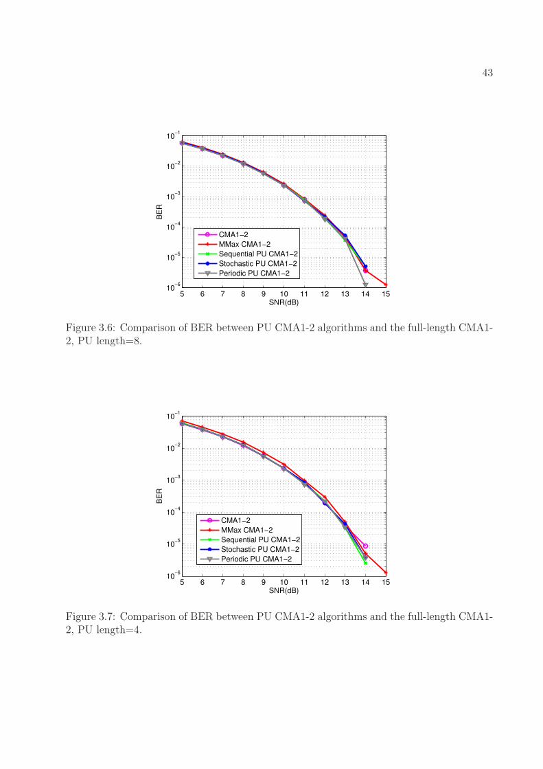
43

5 6 7 8 9 10 11 12 13 14 1510

−6

10−5

10−4

10−3

10−2

10−1

SNR(dB)

BE

R

CMA1−2

MMax CMA1−2



Periodic PU CMA1−2

Figure 3.6: Comparison of BER between PU CMA1-2 algorithms and the full-length CMA1-2, PU length=8.

5 6 7 8 9 10 11 12 13 14 1510

−6

10−5

10−4

10−3

10−2

10−1

SNR(dB)

BE

R

CMA1−2

MMax CMA1−2



Periodic PU CMA1−2

Figure 3.7: Comparison of BER between PU CMA1-2 algorithms and the full-length CMA1-2, PU length=4.

44

5 6 7 8 9 10 11 12 13 14 1510

−6

10−5

10−4

10−3

10−2

10−1

SNR(dB)

BE

R

NCMA

MMax NCMA

Sequential PU NCMA

Stochastic PU NCMA

Periodic PU NCMA

Figure 3.8: Comparison of BER between PU NCMA algorithms and the full-length NCMA,PU length=8.

Fig. 3.8 and Fig. 3.9 illustrate the BER performance of PU NCMA for M = 8 and M = 4,

respectively. For M = 8, the PU NCMA algorithms can obtain similar BER as the NCMA.

However, the PU NCMA perform a little worse than the original NCMA when M = 4.

Fig. 3.10 and Fig. 3.11 illustrate the BER performance between PU LSCMA algorithms

and the full-length LSCMA for M = 8 and M = 4, respectively. For M = 8, the BER

performance of different PU LSCMA algorithms slightly outperforms the full-update LSCMA

when SNR is high. For M = 4, the PU LSCMA can achieve much better BER performance

than the LSCMA at high SNR.

3.5.3 Complexity

Since partial-update methods can reduce the computational complexity in the adaptive al-

gorithm part, the numerical computational complexity of PU CMA algorithms is compared

according to Table 3.1. N is equal to 16. M is equal to 8 and 4, respectively. K in LSCMA

45

5 6 7 8 9 10 11 12 13 14 1510

−6

10−5

10−4

10−3

10−2

10−1

SNR(dB)

BE

R

NCMA

MMax NCMA

Sequential PU NCMA

Stochastic PU NCMA

Periodic PU NCMA

Figure 3.9: Comparison of BER between PU NCMA algorithms and the full-length NCMA,PU length=4.

5 6 7 8 9 10 11 12 13 14 1510

−6

10−5

10−4

10−3

10−2

10−1

100

SNR(dB)

BE

R

LSCMA

MMax LSCMA

Sequential PU LSCMA

Stochastic PU LSCMA

Periodic PU LSCMA

Figure 3.10: Comparison of BER between PU LSCMA algorithms and the full-lengthLSCMA, PU length=8.

46

5 6 7 8 9 10 11 12 13 14 1510

−6

10−5

10−4

10−3

10−2

10−1

100

SNR(dB)

BE

R

LSCMA

MMax LSCMA

Sequential PU LSCMA

Stochastic PU LSCMA

Periodic PU LSCMA

Figure 3.11: Comparison of BER between PU LSCMA algorithms and the full-lengthLSCMA, PU length=4.

is chosen to be 4 times the original equalizer length and is equal to 4 × 16 = 64. Table 3.6

shows the adaptive algorithm complexity for the simulation example.

From the table, PU LSCMA can reduce the number of additions or multiplications about

(N/M)2 times of the LSCMA, while the PU SC-CMA can only reduce the complexity about

N/M times.

Table 3.6: Adaptive Algorithm Complexity

Algorithms CMA1-2 NCMA LSCMAOrg + 67 98 1060

PUL=8 + 35 50 273.5PUL=4 + 17 26 73Org × 70 103 1099.8

PUL=8 × 38 55 293.875PUL=4 × 22 31 84.4375Org SRD 1 1 1.25

PUL=8 SRD 1 1 1.125PUL=4 SRD 1 1 1.0625

47

From the simulations, we draw the following conclusion:

1. PU LSCMA can reduce the number of additions or multiplications by about (N/M)2

times that of the LSCMA. PU CMA1-2 and NCMA can reduce the complexity by

about N/M times.

2. PU CMA algorithms can achieve similar steady-state performance as the original CMA

algorithms.

3. Sequential LSCMA can converge faster than the CMA1-2 and NCMA.

4. PU CMA1-2 and PU NCMA can be used in a real-time processor such as FPGA, and

is suitable for a static channel condition.

3.6 Simulation II – LSCMA Performance using a Real-

istic DSSS System and a Fractionally-Spaced Equal-

izer

The performance of PU LSCMA is simulated in Matlab through a realistic DSSS system

and a fractionally spaced equalizer. The end-to-end system, channel model, and equalizer

model considered in this simulation are shown in Fig. 3.12-3.14. The system is a direct-

sequence spread spectrum (DSSS) system. The channel model is a simplified representation

of a wireless communication link in which a modulated transmitted signal is received in the

presence of additive noise, interference, and correlated multipath due to reception of the

signal over multiple transmission paths. The fractionally-spaced equalizer is a finite impulse

response (FIR) filter, but has different input and output sample rates.

48

Figure 3.12: System model.

Figure 3.13: Channel model.

Figure 3.14: FSE model.

49

The transmitted signal is a pulse-amplitude-modulation (PAM) signal and can be modeled

by

d(t) =∑

n

b(n)pb(t− nTb) (3.78)

pb(t) =Lc−1∑

m=0

c(m)pc(t− nTc), (3.79)

where b(n) is the baseband modulated signal with symbol rate fb = 1/Tb. It is assumed to

be a discrete-time complex signal with a constant modulus, such that |b(n)| ≡ 1 at every

time sample n. Example signals that possess this property include QPSK (4QAM) and PSK

symbol sequences, complex baseband representations of GMSK and FM transmit signals,

and so on. {c(m)}Lc−10 is a spreading sequence, while pc(t) and fc = 1/Tc are the chip

shaping and chip rate of the transmitted signal.

The multipath channel can be modeled by [41]

hc(t, τl, φl) =∑

l

α(φl)ejθlp(t− τl), (3.80)

where α2(φl) is the power of lth multipath component, φl is the angle-of-arrival of the lth

multipath component, θl is the phase of the lth multipath component, p(t) is the pulse, and

τl is the time delay of the lth multipath component.

Assuming that s(n) = b(n)ej2πnfoTb is the transmitted symbol sequence with frequency-offset

fo, the received signal can then be modeled by

x(n) = hs(n) + ε(n), (3.81)

where h is a vector representation of transmit pulse shaping (spreading and chip shaping)

50

and multipath channel effects. ε(n) is the background noise and co-channel interference

(CCI) vector.

Since a fractionally-spaced equalizer is used, the recovered (equalizer output) signal can be

modeled by

y(n) =N−1∑

i=0

wix(nP − i)

= xT (nP )w (3.82)

where w = [ w0 · · · wN−1 ]T is the N×1 equalizer weight vector representation of the FSE

impulse response, and the input sample rate fs equals Pfb, which means the equalizer tap

spacing is 1/P symbols. x(nP ) = [ x(nP ) · · · x(nP −N + 1) ]T is the N × 1 input data

vector to FSE. The goal of the equalizer adaptation algorithm is to design an equalizer weight

vector that can remove the channel and pulse shaping effects. In conventional nonblind

systems, this is typically accomplished by adapting the equalizer to minimize the mean-

square error (MSE) between the equalizer output signal y(n) and the transmitted signal s(n)

over some known component of s(n), e.g., some known training or pilot sequence transmitted

as part of s(n). However, in many applications, such as packet-data and VoIP communication

systems, s(n) may not contain a training sequence that is known at the receiver. Moreover,

even if that sequence is known, the receiver must compensate for the timing and carrier

offset between the transmitter and receiver before that sequence can be used, resulting in a

potentially costly search procedure, and the receiver will not be able to track changes in the

channel over intervals that do not contain that sequence. Lastly, transmission of that training

sequence comes at the cost of traffic capacity. This cost can be prohibitive in highly dynamic

channels (requiring frequent retransmission of training sequences to track channel changes)

or for highly bursty, low capacity communication signals, e.g., data packets providing VoIP

51

Spectral Response of the ADC Output Data

−10 MHz −5 MHz 0 MHz +5 MHz +10 MHz−60 dB

−30 dB

0 dB

+30 dB

+60 dB

+90 dB

Figure 3.15: The spectral response at ADC output.

services. The signal of interest (SOI) is a DSSS waveform based on the 802.11 physical

standard. The baseband modulated signal is a BPSK signal with data rate 1 Mbps. The

spreading code is a 11-length Barker code. The chip shaping code is [0.4, 0.8, 1.0, 0.8, 0.4].

The center frequency of SOI is 2437 MHz. The receive signal-to-white-noise ratio (SWNR) is

0 dB. Meanwhile, two strong interferences are also received at 2437 MHz. The interference

is also a DSSS waveform based on the 802.11 physical standard. It is QPSK modulated

with data rate 2 Mbps. The receive SWNR is 60 dB. The spreading code and chip shaping

are the same as the SOI. Each emission has independent carrier offset and the transmitter

mixer frequency offset is 25 part per million (ppm). In addition, the SOI and interferences

are received with random uniform distributed U(−180o, 180o) phase offsets and random

U(0, 1µs) timing offsets. The ADC sampling rate is 20 Msps. The spectral response at the

ADC output is shown in Fig. 3.15.

Without equalization, the received signal has been corrupted by pulse shaping, inter-symbol-

interference (ISI), CCI, and noise. After applying an FSE, most of the pulse shaping, ISI,

and CCI will be removed. The block size of LSCMA is 160. We set the entire length of the

equalizer to be 40 (N=40), and PU lengths to be 20 (M=20), 10 (M=10), and 8 (M=8),

respectively. In the equalizer part, sequential, and stochastic PU LSCMA algorithms are

52

implemented according to (3.24) and the different PU methods introduced in Section II C.

Note that the MMax LSCMA is also named selective LSCMA in this section. The selective

LSCMA cannot perform as well as the LSCMA and other PU LSCMA algorithms, because

the positions of the weights for updating are almost the same for each update in the FSE with

a cyclostationary input. Only a few weights are updated, and others remain zero. Therefore,

the result is not optimized. Therefore, the selective LSCMA is not presented here. A new PU

method - selective-sequential method is developed for LSCMA to improve the performance

of selective LSCMA in this section. The selective-sequential method combines the selective

method and sequential method. The initial weights equal zero, except there are 5 non-zero

taps in the middle. The 5 non-zero taps are generated by a conjugate self-coherence-restoral

(C-SCORE) algorithm [4]. The BPSK signal is conjugate self-coherent. This algorithm can

detect the 1 Mbps SOI and provide an appropriate initialization for the LSCMA. It is well-

known that the NCMA cannot guarantee convergence to the SOI [49, 25, 17]. Therefore, the

performance of NCMA is not compared with LSCMA. The steady-state constant-modulus-

cost-function (CMCF) and convergence performance are shown. The results are obtained by

averaging 50 independent runs. The total number of symbols is 20000.

3.6.1 Steady-State Performance

Fig. 3.16-3.18 shows the CMCF performance for the sequential, stochastic, and selective-

sequential dynamic LSCMA, respectively. The partial update length is 20, 10, and 8. The

performance is compared with the full-update dynamic LSCMA. The CMCF results are

generated by time-averaging 160 symbols. We can see that the PU dynamic LSCMA can

achieve similar steady-state CMCF as the full-update LSCMA when the PU length is 20 and

10. When the PU length is 8, the PU dynamic LSCMA has not converged to steady state.

The selective dynamic LSCMA (also named MMax LSCMA in this dissertation) does not

53

perform as well as the dynamic LSCMA and other PU dynamic LSCMA algorithms, because

the input signal in this example is a cyclostationary signal. The positions of the weights for

updating are almost the same for each update. To improve the performance of selective

LSCMA, we combine the selective method with the sequential method. First, a sorting step

is done like the selective method. Since the positions are barely changed for LSCMA FSE

with a cyclostationary signal, we use the sequential method after the sorting step. For the

first iteration, the positions of the M largest elements are chosen. For the second iteration,

the positions of the M less largest elements are chosen, and so on. The purpose of including a

sequential method is to update all the weights so that the selective LSCMA does not update

the same weights at each iteration, which can cause convergence problems. Fig. 3.19 shows

the histogram plot of the number of updates versus weight position for sequential, stochastic,

selective, and selective-sequential LSCMA for a single run. The partial update length is

16. We can see that the sequential method updates weight positions evenly, the stochastic

and selective-sequential methods update weight positions almost evenly, and the selective

LSCMA updates the same weight positions for each iteration. Both dynamic LSCMA and

PU dynamic LSCMA have lower CMCF than the NCMA and PU NCMA.

3.6.2 Convergence Performance

The convergence performance is shown by using the delay-compensated SINR performance.

The SINR is defined as the inverse of the gain-optimized normalized mean-square-error

(NMSE), which is

SINR(∆) =1

NMSE(∆)− 1. (3.83)

54

2 ms 4 ms 6 ms 8 ms 10 ms 12 ms 14 ms 16 ms 18 ms−18 dB

−16 dB

−14 dB

−12 dB

−10 dB

−8 dB

−6 dB

−4 dBC

MC

F

MMSE

LSCMA

Sequential LSCMA M=20



Figure 3.16: The CMCF performance of the sequential dynamic LSCMA.


−16 dB

−14 dB

−12 dB

−10 dB

−8 dB

−6 dB

−4 dB

CM

CF

MMSE

LSCMA

Stochastic LSCMA M=20



Figure 3.17: The CMCF performance of the stochastic dynamic LSCMA.

55


−16 dB

−14 dB

−12 dB

−10 dB

−8 dB

−6 dB

−4 dB

CM

CF

MMSE

LSCMA

Selective−sequential LSCMA M=20



Figure 3.18: The CMCF performance of the selective-sequential dynamic LSCMA.

10 20 30 40 50 600

20

40

Weight position i

Nu

mb

er

of

ud

pa

tes Sequential LSCMA, M=16

10 20 30 40 50 600

20

40

Weight position i

Nu

mb

er

of

ud

pa

tes Stochastic LSCMA, M=16

10 20 30 40 50 600

20

40

Weight position i

Nu

mb

er

of

ud

pa

tes Selective LSCMA, M=16

10 20 30 40 50 600

20

40

Weight position i

Nu

mb

er

of

ud

pa

tes Selective−sequential LSCMA, M=16

Figure 3.19: The histogram plot of the number of updates versus weight position, PU dy-namic LSCMA, PU length=16.

56

The NMSE is defined as

NMSE(∆) = 1− |〈y(n)s∗(n−∆)〉|2

〈|y(n)|2〉〈|s(n−∆)|2〉, (3.84)

where y(n) is the equalizer output, s(n−∆) is the delayed transmitted signal, and ∆ is the

number of the delay.

Figs. 3.20 - 3.22 show the SINR results of PU dynamic LSCMA. The SINR results are

generated by by using a priori output (y = X(q)w(q)) and for each block with 160 symbols.

We define the target bit-error-rate (BER) capture time as the time when SINR reaches 6.8

dB, which yields 10−3 BER for a BPSK signal. The capture time of PU LSCMA increases

as the PU length reduces. From Fig. 3.20 - 3.22, we can see that the sequential LSCMA

can capture 6.8 dB SINR with less time than the other two PU methods. Note that since

the stochastic method chooses the update weights randomly, the capture time may change

dramatically. Delay in this example is zero symbols for all the data blocks and for all the

algorithms.

The dynamic LSCMA using a posteriori output (y = X(q)w(q+1)) can achieve higher SINR

than the dynamic LSCMA using a priori output, even in steady state. It can also increase

the convergence rate. Using the same convergence analysis method as Section IV B, we can

show that

JpS(q) = ‖sp(q)− yp(q)‖2

≤ JS(q)− ‖yp(q)− y(q)‖2 (3.85)

≤ JS(q), (3.86)

57

0 ms 5 ms 10 ms 15 ms 20 ms0 dB

2 dB

4 dB

6 dB

8 dB

10 dB

12 dB

14 dB

SIN

R

MMSE

LSCMA




MMSE delay = 0 symbol

MMSE delay = −1 symbol

SINR=6.8 dB

Figure 3.20: The SINR performance of the sequential dynamic LSCMA.

0 ms 5 ms 10 ms 15 ms 20 ms0 dB

2 dB

4 dB

6 dB

8 dB

10 dB

12 dB

14 dB

SIN

R

MMSE

LSCMA






SINR=6.8 dB

Figure 3.21: The SINR performance of the stochastic dynamic LSCMA.

58

0 ms 5 ms 10 ms 15 ms 20 ms0 dB

2 dB

4 dB

6 dB

8 dB

10 dB

12 dB

14 dB

SIN

R

MMSE

LSCMA






SINR=6.8 dB

Figure 3.22: The SINR performance of the selective-sequential dynamic LSCMA.

where yp is the a posteriori output, y is the a priori output, JpS is the CMCF of the a

posteriori output, and JS is the CMCF of the a priori output. We can see that the CMCF of

the a posteriori output is always smaller than the CMCF of the a priori output if ‖yp(q)−

y(q)‖2 6= 0. When ‖yp(q) − y(q)‖2 = 0, the a posteriori CMCF is equal to the a priori

CMCF. One solution of ‖yp(q) − y(q)‖2 = 0 is that {|yk(q)|}Kk=1 = {1}, which is hard to

be achieved in a noise environment. Note that the steady-state analysis of the a posteriori

CMCF will be different from the analysis of the a priori CMCF in this section.

Figs. 3.23 - 3.25 show the SINR results by using the a posteriori output for each block with

160 symbols. We can see that the dynamic LSCMA converges to the MMSE solution quickly.

The PU dynamic LSCMA using the a posteriori output can also perform better than the

equivalent algorithm using the a priori output, but not as well as the full-update dynamic

LSCMA. This is because the PU LSCMA only updates a few weights for each iteration, and

the a posteriori output does not vary significantly from the a priori output, especially when

the PU length reduces.

Table 3.7 shows the average target bit-error-rate (BER) capture time over 100 runs for PU

59

0 ms 5 ms 10 ms 15 ms 20 ms0 dB

2 dB

4 dB

6 dB

8 dB

10 dB

12 dB

14 dB

SIN

R

MMSE

LSCMA






SINR=6.8 dB

Figure 3.23: The SINR performance of the sequential dynamic LSCMA using the a posteriorioutput.

0 ms 5 ms 10 ms 15 ms 20 ms0 dB

2 dB

4 dB

6 dB

8 dB

10 dB

12 dB

14 dB

symbols

SIN

R

MMSE

LSCMA






SINR=6.8 dB

Figure 3.24: The SINR performance of the stochastic dynamic LSCMA using the a posteriorioutput.

60

0 ms 5 ms 10 ms 15 ms 20 ms0 dB

2 dB

4 dB

6 dB

8 dB

10 dB

12 dB

14 dB

SIN

R

MMSE

LSCMA





SINR=6.8 dB


Figure 3.25: The SINR performance of the selective-sequential dynamic LSCMA using thea posteriori output.

dynamic LSCMA by using the a priori output and the a posteriori output. The average

capture time by using the a posteriori output is less than the average capture time by using

the a priori output. The actual target BER capture time for each run is different from

the average target BER capture time. Figs. 3.26 - 3.29 show the confidence of the average

target BER capture time, which is how many runs within the 100 runs can achieve 6.8 dB

SINR at the average target BER capture time. The performance of various PU methods

are different. Fig. 3.26 shows the performance of full-update LSCMA with both a priori

output and a posteriori output. The average target BER capture time of the full-update

LSCMA with a priori output is 640 samples and its confidence is 73%. The average target

BER capture time of the full-update LSCMA with a posteriori output is 640 samples and its

confidence is 79%. Fig. 3.27 shows the performance of sequential LSCMA for both a priori

output and a posteriori output. Since the sequential method is a deterministic method, the

overall confidence of target BER capture time is high. Fig. 3.28 shows the performance of

stochastic LSCMA for both a priori output and a posteriori output. The overall confidence

61

Table 3.7: Average Target BER Capture Time of PU dynamic LSCMA

Algorithms Target BER capture time (samples)a priori output a posteriori output

LSCMA, N=40 640 480Sequential 960 640

LSCMA, M=20Sequential 1600 1440

LSCMA, M=10Sequential 1920 1760

LSCMA, M=8Stochastic 1280 1120



LSCMA, M=8Selective-sequential 1120 800LSCMA, M=20

Selective-sequential 3520 2720LSCMA, M=10

Selective-sequential 5760 5600LSCMA, M=8

of stochastic is around 50% since the target BER capture time changes dramatically for

stochastic method for different runs. Fig. 3.29 shows the performance of selective-sequential

LSCMA for both a priori output and a posteriori output. The confidence varies for different

PU length.

The convergence performance of static LSCMA and PU static LSCMA is shown in Fig. 3.30.

The PU length is 20. The static LSCMA can achieve the MMSE solution after 10 updates.

Since static LSCMA uses the entire input data to estimate the auto-correlation matrix, not

a finite-length data window, it can converge to the MMSE solution. The PU static LSCMA

can achieve similar SINR when the number of updates increases. The static LSCMA can

reach 6.8 dB SINR after 3 updates. The sequential static LSCMA needs 4 updates. The

62

500 1000 1500 2000 2500 30000

10

20

30

40

50

60

70

80

90

100

Samples

Confidence (

%)

LSCMA with a priori output

LSCMA with a posteriori output

Average target BER capture time = 640


Figure 3.26: The confidence of the average target BER capture time for LSCMA.

500 1000 1500 2000 2500 3000 3500 4000 45000

10

20

30

40

50

60

70

80

90

100

Samples

Co

nfid

en

ce

(%

)

Sequential LSCMA with a priori output, M=20



Sequential LSCMA with a posteriori output, M=20









Figure 3.27: The confidence of the average target BER capture time for sequential LSCMA.

63

2000 4000 6000 8000 10000 12000 14000 160000

10

20

30

40

50

60

70

80

90

100

Samples

Confidence (

%)

Stochastic LSCMA with a priori output, M=20



Stochastic LSCMA with a posteriori output, M=20









Figure 3.28: The confidence of the average target BER capture time for stochastic LSCMA.

1000 2000 3000 4000 5000 6000 7000 8000 90000

10

20

30

40

50

60

70

80

90

100

Samples

Co

nfid

en

ce

(%

)

1000 2000 3000 4000 5000 6000 7000 8000 90000

10

20

30

40

50

60

70

80

90

100

Samples

Co

nfid

en

ce

(%

)

Selective−sequential a priori LSCMA M=20



Selective−sequential a posteriori LSCMA M=20















Figure 3.29: The confidence of the average target BER capture time for selective-sequentialLSCMA.

64

10 20 30 40 50 600 dB

2 dB

4 dB

6 dB

8 dB

10 dB

12 dB

14 dB

Number of update

SIN

R

MMSE

LSCMA






SINR=6.8 dB

3 updates

4 updates

5 updates

Figure 3.30: The SINR performance for static LSCMA and PU static LSCMA, PUlength=20.

stochastic and selective-sequential static LSCMA need 5 updates to reach 6.8 dB SINR. The

performance of static LSCMA and PU static LSCMA using the a posteriori output is shown

in Fig. 3.31. Using the a posteriori output, the steady-state SINR does not change, but

the target BER capture time is reduced. The static LSCMA needs 2 updates to reach 6.8

dB SINR. The sequential LSCMA needs 3 updates. The stochastic and selective-sequential

needs 4 updates to reach 6.8 dB SINR.

3.6.3 Complexity and Simulation Time

The numerical computational complexity of dynamic LSCMA and PU dynamic LSCMA

are calculated from Table 3.1, where N is equal to 40, and M is equal to 20, 10, and 8,

respectively. K in dynamic LSCMA is chosen to be 4 times the original equalizer length and

is equal to 4× 40 = 160.

Table 3.8 shows the total DSP cycles (including adaptive algorithm complexity and filter

65

10 20 30 40 50 600 dB

2 dB

4 dB

6 dB

8 dB

10 dB

12 dB

14 dB

Number of update

SIN

R

MMSE

LSCMA






SINR=6.8 dB

4 updates

3 updates

2 updates

Figure 3.31: The SINR performance for static LSCMA and PU static LSCMA using the aposteriori output, PU length=20.

complexity) needed to achieve 6.8 dB SINR using the a priori output. Number of total cycles

is represented in million (M). From the table, we can see that the PU dynamic LSCMA needs

fewer DSP cycles than the dynamic LSCMA. The sequential LSCMA needs fewer DSP cycles

than the other PU LSCMA.

Table 3.9 shows the total DSP cycles needed to achieve 6.8 dB SINR by using the a posteriori

output. The full-update LSCMA using the a posteriori output needs fewer DSP cycles to

achieve the target BER capture SINR. The PU dynamic LSCMA using the a posteriori also

needs fewer DSP cycles to achieve the target BER capture SINR when PU length is large.

However, when PU length is short, the reduction in capture time may not be worth the

increased complexity cost.

For static LSCMA with the a priori output, the full update method needs 6687∗20000∗3 =

401.22M cycles to reach 6.8 dB SINR, while the sequential static LSCMA with PU length

20 needs 1987 ∗ 20000 ∗ 4 = 146.24M cycles. The PU method can save about 2.7 times DSP

cycles for static LSCMA. For static LSCMA with the a posteriori output, the full update

66

Table 3.8: Complexity over average target BER capture time using a priori output

Algorithms Cycles/sample Average target BER Total cyclescapture time

LSCMA, N=40 6702 640 4.29MSequential 1832 960 1.76M

LSCMA, M=20Sequential 599 1600 0.96M


LSCMA, M=8Stochastic 1832 1280 2.34M



LSCMA, M=8Selective-sequential 1832 1120 2.05MLSCMA, M=20

Selective-sequential 599 3520 2.10MLSCMA, M=10


67

Table 3.9: Complexity over target BER capture time using a posteriori output

Algorithms Cycles/sample Target BER Total cyclescapture time

LSCMA, N=40 6861 480 3.29MSequential 1991 640 1.27M






LSCMA, M=8Selective-sequential 1991 800 1.59MLSCMA, M=20



68

Table 3.10: Overall simulation time for dynamic LSCMA

Algorithms Simulation time (s)LSCMA 0.65586

Sequential LSCMA, M=20 0.1841Stochastic LSCMA, M=20 0.3585

Selective-sequential LSCMA, M=20 0.19952Sequential LSCMA, M=10 0.075204Stochastic LSCMA, M=10 0.14972

Selective-sequential LSCMA, M=10 0.087077Sequential LSCMA, M=8 0.061805Stochastic LSCMA, M=8 0.11968

Selective-sequential LSCMA, M=8 0.074771

method needs 6846 ∗ 20000 ∗ 2 = 273.84M cycles to reach 6.8 dB SINR, while the sequential

static LSCMA with PU length 20 needs 1828 ∗ 20000 ∗ 3 = 119.22M cycles. The PU method

can also save about 2.3 times DSP cycles for static LSCMA.

Table 3.10 shows the overall simulation time per run in Matlab for dynamic LSCMA and PU

dynamic LSCMA using a priori output. The results show that the PU LSCMA can reduce

the simulation time significantly.

3.7 Algorithm Analysis for a Time-Varying System

In real world applications, the unknown system is usually time-varying. Therefore, tracking

analysis is needed to show how well an adaptive filter performs in a time-varying environment.

The optimal weights wo become wo(n), i.e. they change with time.

A first-order Markov model [43] is used for the time-varying unknown system. It has a form

as follows:

wo(n) = wo(n− 1) + η(n), (3.87)

69

where η(n) is the process noise vector with zero mean and correlation matrix Rη = E{ηHη}.

To determine the tracking performance, another assumption is needed: η(n) is independent

of all other signals.

The coefficient error in the tracking analysis is defined

z(n) = wo(n)−w(n). (3.88)

3.7.1 Algorithm Analysis of CMA1-2 and NCMA for a Time-

Varying System

Use the same analyses in time-invariant section 3.4.1. The coefficient error of CMA1-2 in

(3.33) becomes

z(n+ 1) = z(n) + η(n+ 1) + µx∗(n)v(n)− µx∗(n)xT (n)z(n). (3.89)

Take the expectation of (3.89). Since E{v} = 0, E{z} = 0, and E{η} = 0, the average

weights still converge to the optimal weights at steady state. The convergence condition is

0 < µ <2

βλmax(E{x∗xT}) , (3.90)

β ≈ MN, for sequential and stochastic methods

MN

< β < 1, for MMax method(3.91)

70

Following the analyses from (3.39) to (3.42), the steady-state MSE of PU CMA1-2 in a

time-varying system becomes

E{|e(n)|2} = σ2v +

µσ2vE{‖x‖2}+ µ−1E{‖η‖2}

2β − µE{‖x‖2} , n→∞. (3.92)

Assuming the process noise is white with variance σ2η, the steady-state MSE of PU CMA1-2

in a time-varying system can be simplified as

E{|e(n)|2} = σ2v +

µσ2vE{‖x‖2}+ µ−1Nσ2

η

2β − µE{‖x‖2} , n→∞. (3.93)

For PU NCMA, the convergence in the mean is achieved if 0 < µ < 2. The steady-state

MSE of PU NCMA in a time-varying system becomes

E{|e(n)|2} = σ2v +

µσ2v + µ−1tr(RηE{xH x})

2− µ, n→∞. (3.94)

If white process noise is used, it can be simplified as

E{|e(n)|2} = σ2v +

µσ2v + µ−1σ2

ηE{‖x‖2}2− µ

, n→∞. (3.95)

3.7.2 Algorithm Analysis of LSCMA for a Time-Varying System

Use the same analyses in time-invariant section 3.4.2. The coefficient error of LSCMA in

(3.50) becomes

z(q + 1) = z(q) + η(q + 1) + X†(q)v(q)− X†(q)X(q)z(q). (3.96)

71

Take the expectation of (3.96). Since E{v} = 0, E{z} = 0, and E{η} = 0, the average

weights still converge to the optimal weights at steady state. Convergence in the mean is

achieved if the inversion of E{X†X} exists, which means E{X†X} has full rank and it is

nonsingular. Again, follow the analyses from (3.53) to (3.60), the steady-state MSE of PU

LSCMA in a time-varying system becomes

E{|e(q)|2} = Kσ2v +

σ2vtr(|E{A}|) + tr(RηE{XHX})(tr(|E{B}|)− tr(|E{A}|)) , n→∞. (3.97)

Since the cost function of LSCMA is based on an output vector with length K, the block-

based MSE can be revised to the sample-based MSE as

E{|e(q)|2} = σ2v +

σ2vtr(|E{A}|) + tr(RηE{XHX})K(tr(|E{B}|)− tr(|E{A}|)) , n→∞. (3.98)

If the white process noise is used, it can be simplified as

E{|e(q)|2} = σ2v +

σ2vtr(|E{A}|) + σ2

ηtr(E{XHX})K(tr(|E{B}|)− tr(|E{A}|)) , n→∞. (3.99)

3.7.3 Simulation

The same simulation example as in section 3.5 is used, except the FIR channel changes with

time. The process noise is white noise with ση = 0.001 and ση = 0.0001. SNR is 15 dB. The

results are obtained by averaging 100 independent runs.

Fig. 3.32 shows the CMCF performance for PU CMA1-2 with PU length M = 8 and

ση = 0.001. The MMax, sequential, and stochastic CMA1-2 perform similar to the full-

update CMA1-2 at steady state. Fig. 3.33 shows the CMCF performance for PU CMA1-2

with PU length M = 4 and ση = 0.001. In this case, the MMax, sequential, and stochastic

72

0 1000 2000 3000 4000 5000 6000 7000 8000 90000

0.1

0.2

0.3

0.4

0.5

0.6

0.7

0.8

0.9

1

Iteration (n)

J(n

)

CMA1−2

MMax CMA1−2

Sequential CMA1−2

Stochastic CMA1−2

Figure 3.32: The CMCF performance for PU CMA1-2 for a time-varying system, PUlength=8, ση = 0.001.

CMA1-2 perform worse than the full-update CMA1-2. This is because the process noise

dominates the MSE and it increases as the PU length reduces according to the theoretical

results. Step size µ is 0.0025 for ση = 0.001. Fig. 3.34 shows the CMCF performance for

PU CMA1-2 with PU length M = 8 and ση = 0.0001. All the PU CMA1-2 and the original

CMA1-2 have similar steady-state performance. Fig. 3.35 shows the CMCF performance

for PU CMA1-2 with PU length M = 4 and ση = 0.0001. Again, all the PU CMA1-2 and

the original CMA1-2 have similar steady-state performance. Comparing Fig. 3.34 and Fig.

3.35 with Fig. 3.32 and Fig. 3.33, we can see that the CMCF increases as the process noise

increases. Step size µ for ση = 0.0001 is 0.005.

Fig. 3.36 shows the CMCF performance for PU NCMA with PU length M = 8 and ση =

0.001. Fig. 3.37 shows the CMCF performance for PU NCMA with PU length M = 4 and

ση = 0.001. The sequential and stochastic NCMA have the lower CMCF than the full-update

NCMA in these two cases. This is because the steady-state MSE of PU NCMA is related

to E{‖x‖2}. The average norm-square of the sequential and stochastic PU input vector is

73

0 1000 2000 3000 4000 5000 6000 7000 8000 90000

0.1

0.2

0.3

0.4

0.5

0.6

0.7

0.8

0.9

1

Iteration (n)

J(n

)

CMA1−2

MMax CMA1−2

Sequential CMA1−2

Stochastic CMA1−2


0 1000 2000 3000 4000 5000 6000 7000 8000 90000

0.1

0.2

0.3

0.4

0.5

0.6

0.7

0.8

0.9

1

Iteration (n)

J(n

)

CMA1−2

MMax CMA1−2

Sequential CMA1−2

Stochastic CMA1−2


74

0 1000 2000 3000 4000 5000 6000 7000 8000 90000

0.1

0.2

0.3

0.4

0.5

0.6

0.7

0.8

0.9

1

Iteration (n)

J(n

)

CMA1−2

MMax CMA1−2

Sequential CMA1−2

Stochastic CMA1−2


smaller than the average norm-square of the full-update input vector. When process noise is

big, the steady-state MSE of the sequential and stochastic NCMA is smaller than the full-

update NCMA. The step size µ in the case ση = 0.001 is 0.01. Fig. 3.38 shows the CMCF

performance for PU NCMA with PU length M = 8 and ση = 0.0001. Fig. 3.39 shows the

CMCF performance for PU NCMA with PU length M = 4 and ση = 0.0001. The step size µ

in the case ση = 0.0001 is 0.01. Since the process noise is very small, the performance of PU

length 4 is similar to that of PU length 8, and the performance of PU NCMA is similar to

full-update NCMA at steady state. Decreasing the PU length does not necessarily decrease

the performance.

Fig. 3.40 shows the CMCF performance for PU LSCMA with PU length M = 8 and

ση = 0.001. In this case, the PU LSCMA has similar performance to the full-update LSCMA.


ση = 0.001. The PU LSCMA still has similar steady-state MSE as the full-update LSCMA.


75

0 2000 4000 6000 8000 100000

0.1

0.2

0.3

0.4

0.5

0.6

0.7

0.8

0.9

1

Iteration (n)

J(n

)

NCMA

MMax NCMA

Sequential NCMA

Stochastic NCMA

Figure 3.36: The CMCF performance for PU NCMA for a time-varying system, PUlength=8, ση = 0.001.

0 2000 4000 6000 8000 100000

0.1

0.2

0.3

0.4

0.5

0.6

0.7

0.8

0.9

1

Iteration (n)

J(n

)

NCMA

MMax NCMA

Sequential NCMA

Stochastic NCMA


76

0 2000 4000 6000 8000 100000

0.1

0.2

0.3

0.4

0.5

0.6

0.7

0.8

0.9

1

Iteration (n)

J(n

)

NCMA

MMax NCMA

Sequential NCMA

Stochastic NCMA


0 2000 4000 6000 8000 100000

0.1

0.2

0.3

0.4

0.5

0.6

0.7

0.8

0.9

1

Iteration (n)

J(n

)

NCMA

MMax NCMA

Sequential NCMA

Stochastic NCMA


77

0 2000 4000 6000 8000 100000

0.1

0.2

0.3

0.4

0.5

0.6

0.7

0.8

0.9

1

Iteration (n)

J(n)

LSCMA

MMax LSCMA

Sequential PU LSCMA

Stochastic PU LSCMA

Figure 3.40: The CMCF performance for PU dynamic LSCMA for a time-varying system,PU length=8, ση = 0.001.

ση = 0.0001. Fig. 3.43 shows the CMCF performance for PU LSCMA with PU lengthM = 4

and ση = 0.0001. Since the process noise is small, the PU LSCMA has similar steady-state

performance to the full-update LSCMA. We can see that the CMCF increases as the process

noise increases. Since the PU LSCMA can achieve similar tracking performance as the full-

update LSCMA while reducing the computational complexity significantly, it is suitable for

systems with dynamic environments.

The steady-state results at PU length is equal to 4 are more fuzzy than those at PU length

is equal to 8 for all the PU CMA-based algorithms. This is because tracking performance

is a non-stationary system and the temporal variance of MSE increases as the degree of

non-stationary increases [22].

Tables 3.11 and 3.12 show the theoretical and simulated MSE for PU CMA algorithms when

ση = 0.001 and ση = 0.0001, respectively. Two cases, PU length is equal to 8 (M = 8) and

PU length is equal to 4 (M = 4), are shown. The theoretical results are calculated by (3.93),

78

0 2000 4000 6000 8000 100000

0.1

0.2

0.3

0.4

0.5

0.6

0.7

0.8

0.9

1

Iteration (n)

J(n)

LSCMA

MMax LSCMA

Sequential PU LSCMA

Stochastic PU LSCMA


0 2000 4000 6000 8000 100000

0.05

0.1

0.15

0.2

0.25

0.3

0.35

0.4

Iteration (n)

J(n

)

LSCMA

MMax LSCMA

Sequential PU LSCMA

Stochastic PU LSCMA


79

0 2000 4000 6000 8000 100000

0.05

0.1

0.15

0.2

0.25

0.3

0.35

0.4

Iteration (n)

J(n

)

LSCMA

MMax LSCMA

Sequential PU LSCMA

Stochastic PU LSCMA


(3.95), and (3.99). We can see that the simulated results match the theoretical results.

3.8 Conclusion

In this chapter, PU methods are applied to the CMA-based algorithms including CMA1-

2, NCMA, and LSCMA. Theoretical mean and mean-square performance are derived for

both time-invariant and time-varying systems. The performance of different PU CMA-based

algorithms are compared by using computer simulations. The simulated results match the

theoretical results. The PU CMA-based algorithms can achieve steady-state MSE similar to

the full-update CMA-based algorithms in a time-invariant system and a simple FIR channel.

Among different PU methods, the MMax method usually has a convergence rate very close

to the full-update method. The sequential and stochastic methods usually converge slower

than the MMax method. However, the MMax method does not always perform well with the

LSCMA algorithm. When the PU length is short, the MMax LSCMA has slow convergence

80

Table 3.11: Steady-State MSE Comparison among Different PU CMA algorithms for a time-varying system, ση = 0.001


CMA1-2 -12.997 -12.345MMax CMA1-2 -12.115 -11.703


PU length=4CMA1-2 -11.885 -11.563


PU length=8NCMA -13.421 -12.843


PU length=4NCMA -11.217 -11.034




PU length=4LSMCA -12.239 -12.239


81

Table 3.12: Steady-State MSE Comparison among Different PU CMA algorithms for a time-varying system, ση = 0.0001


CMA1-2 -16.159 -16.464MMax CMA1-2 -16.239 -16.416


PU length=4CMA1-2 -16.388 -17.073


PU length=8NCMA -13.824 -13.978


PU length=4NCMA -13.871 -13.843






82

rate or does not converge in an FSE system. The sequential LSCMA usually has the best

performance among the PU LSCMA algorithms. A new PU method combining the MMax

method and sequential method, the selective-sequential method, is therefore developed for

LSCMA. It performs well especially for the static LSCMA. The PU NCMA algorithms may

perform better than the full-update NCMA algorithm in tracking a time-varying system.

The PU LSCMA can achieve similar tracking performance as the full-update LSCMA while

reduce the computational complexity significantly, it is suitable for systems with dynamic

environments.

Chapter 4

Partial Update CG Algorithms for

Adaptive Filtering

In this chapter, partial update techniques are applied to the CG algorithm. CG solves the

same cost function as the RLS algorithm. It has a fast convergence rate and can achieve

the same mean-square performance as RLS at steady state. It has lower computational

complexity when compared with the RLS algorithm. The basic partial update methods

such as sequential PU, stochastic PU, and MMax update method, are applied to the CG

algorithm. There is another PU method, periodic method, which updates the adaptive filter

periodically. Since the steady-state performance of the periodic method is the same as the

full-update method, it is not considered here. The mean and mean-square performance of

different PU CG for a time-invariant system are analyzed and compared with the full-update

CG algorithm. The goal of this chapter is to find one or more PU CG algorithms which

can reduce the computational complexity while maintaining good performance. The tracking

performance of the PU CG for a time-varying system is also studied. Theoretical MSE results

are derived for the PU CG at steady state. Computer simulation results are also presented

83

84

to show the tracking performance of the MMax CG. The performance of the MMax CG

is also compared with the full-update CG, full-update RLS, and MMax RLS. The analysis

of time-varying systems is necessary because the unknown systems in system identification,

echo cancellation, and channel equalization are often time-varying in real world applications.

In Section 1, different PU CG algorithms are developed. Theoretical mean and mean-square

analyses of PU CG for a time-invariant system are given in Section 2. Theoretical mean-

square analysis of PU CG for a time-varying system is given in Section 3. In Section 4,

computer simulation results are shown. The performance of different PU CG algorithms are

compared. The performance of PU CG, PU RLS, and PU EDS are also compared.

4.1 Review of Conjugate Gradient Algorithm

In this chapter, only the CG with the non-reset Polak-Ribiere (PR) method is considered

since the CG algorithm with the reset method needs higher computational complexity than

the non-reset method. The CG with the PR method [7] is summarized as follows:

Initial conditions:

w(0) = 0, R(n) = 0, p(1) = g(0).

85

e(n) = d(n)− xT (n)w(n− 1), (4.1)

R(n) = λR(n− 1) + x(n)xT (n), (4.2)

α(n) = ϕpT (n)g(n− 1)

pT (n)R(n)p(n), (4.3)

w(n) = w(n− 1) + α(n)p(n), (4.4)

g(n) = λg(n− 1)− α(n)R(n)p(n) + x(n)e(n), (4.5)

β(n) =(g(n)− g(n− 1))Tg(n)

gT (n− 1)g(n− 1), (4.6)

p(n+ 1) = g(n) + β(n)p(n), (4.7)

where R is the time-average correlation matrix of x, p is the search direction, and g is the

residue vector which is also equal to b(n)−R(n)w(n), where b(n) = λb(n− 1) + x(n)d(n)

is the estimated crosscorrelation of x and d. The choice of g(0) can be d(1)x(1) or satisfies

gT (0)g(0) = 1. λ is the forgetting factor and the constant parameter η satisfies λ − 0.5 ≤

η ≤ λ.

86

4.2 Partial Update CG

The partial update CG algorithm is summarized as follows:

e(n) = d(n)− xT (n)w(n− 1), (4.8)

R(n) = λR(n− 1) + x(n)xT (n), (4.9)

α(n) = ϕpT (n)g(n− 1)

pT (n)R(n)p(n), (4.10)

w(n) = w(n− 1) + α(n)p(n), (4.11)

g(n) = λg(n− 1)− α(n)R(n)p(n) + x(n)e(n), (4.12)

β(n) =(g(n)− g(n− 1))Tg(n)

gT (n− 1)g(n− 1), (4.13)

p(n+ 1) = g(n) + β(n)p(n), (4.14)

where

x = IMx, (4.15)

and

IM(n) =

i1(n) 0 . . . 0

0 i2(n). . .

...

.... . . . . . 0

0 . . . 0 iN(n)

, (4.16)

N∑

k=1

ik(n) = M, ik(n) ∈ {0, 1}, (4.17)

87

Table 4.1: The computational complexities of PU CG for real signals.

Algorithms Number of multiplications Number of additions comparisonsper sample per sample

CG 3N2 + 10N + 3 2N2 + 8N − 3 0Sequential CG 2N2 +M2 + 9N +M + 3 N2 +M2 + 8N − 3 0Stochastic CG 2N2 +M2 + 9N +M + 5 N2 +M2 + 8N − 1 0MMax CG 2N2 +M2 + 9N +M + 3 N2 +M2 + 8N − 3 2 ⌈log2N⌉+ 2

Table 4.2: The computational complexities of PU CG for complex signals.


CG 10N2 + 38N + 10 10N2 + 43N 0Sequential CG 6N2 + 4M2 + 34N + 4M + 10 5N2 + 5M2 + 40N + 3M 0Stochastic CG 6N2 + 4M2 + 34N + 4M + 12 5N2 + 5M2 + 40N + 3M + 2 0MMax CG 6N2 + 4M2 + 36N + 4M + 10 5N2 + 5M2 + 41N + 3M 2 ⌈log2N⌉+ 2

For each iteration, only M elements of the input vector are used to update the weights.

Note, the calculation of the output signal error still uses the the entire input vector, not the

subselected input vector.

The computational complexity of different PU CG for real signals is shown in Table 4.1. The

MMax CG uses the SORTLINE sorting method and introduces 2 ⌈log2N⌉ + 2 comparisons

[11]. The sequential method does not need extra additions or multiplications. The stochastic

CG uses the linear congruential generator and introduces 2 extra multiplications and 2 extra

additions [11]. Table 4.2 shows the computational complexity of different PU CG for complex

signals.

88

4.3 Steady-State Performance of Partial Update CG

for a Time-Invariant System

The normal equation of the partial update CG algorithm can be represented as:

XTM(n)Λ(n)X(n)w(n) = XT

M(n)Λ(n)d(n), (4.18)

where d(n) = [d(n), d(n− 1), . . . , d(1)]T ,

XM(n) =

xTM(n)

xTM(n− 1)

...

xTM(1)

, (4.19)

and

Λ(n) =

1 0 . . . 0

0 λ. . .

...

.... . . . . . 0

0 . . . 0 λn

. (4.20)

Therefore, the residue vector g can also be written as

g = b(n)− R(n)w(n), (4.21)

89

where

R(n) = λR(n− 1) + x(n)xT (n), (4.22)

b(n) = λb(n− 1) + x(n)d(n). (4.23)

To simplify the analysis, we assume that the input signal is wide-sense stationary and ergodic,

and α(n), β(n), R(n), and w(n) are uncorrelated to each other [7]. Apply the expectation

operator to (4.11), (4.12), and (4.14). Define E{α(n)} = α, E{β(n)} = β, E{b(n)} = b,

and E{R(n)} = R. The system can be viewed as linear and time invariant at steady state.

Therefore, the Z -transform can be applied to the system. Define W(z) = Z {E{w(n)}},

G(z) = Z {E{g(n)}}, and P(z) = Z {E{p(n)}}. Equations (4.11), (4.12), and (4.14)

become

W(z) = W(z)z−1 + αP(z), (4.24)

G(z) = λG(z)z−1 − αRP(z)− RW(z)z−1 +bz

z − 1, (4.25)

zP(z) = G(z) + βP(z). (4.26)

Therefore,

W(z) = {[(z − 1)(z − β)I+ αRz](z − 1) + αRz}−1αbz3

z − 1. (4.27)

Since the system is causal and n ≥ 0, the Z -transform is one-sided and W(z) = W+(z).

At steady state, the mean of the weights converges to

limn→∞

E{w(n)} = limz→1

W+(z) = R−1b. (4.28)

90

For the causal system to be stable, all the poles must be inside the unit circle. Therefore,

the conditions for the stability are |β| < 1, λmin > 0, and 0 ≤ α ≤ 2(1+λ)(β+1)

2λmax−λmin

, where λmax

is the maximal eigenvalue of R and λmin is the minimal eigenvalue of R. For the sequential

and stochastic methods, the partial update correlation matrix R may become ill-conditioned

and the condition λmin > 0 cannot be satisfied, especially when M becomes smaller, and the

algorithm may suffer convergence difficulty.

Since the input noise v(n) is assumed to be zero mean white noise and independent of the

input signal x(n), the MSE equation of the PU CG algorithm becomes

E{|e(n)|2} = σ2v + tr(RE{ǫ(n)ǫT (n)}), (4.29)

where σ2v = E{v2(n)} is the variance of the input noise, and ǫ(n) = w∗ − w(n) is the

weight error vector. To simplify the analysis, it is also assumed that the weight error ǫ(n) is

independent of the input signal x(n) at steady state.

At steady state,

w(n) ≈ R−1(n)b(n). (4.30)

Using (4.22), (4.23), and (2.1), w(n) can be written as

w(n) ≈ w∗ + R−1(n)n∑

i=1

λn−ix(i)v(i). (4.31)

Define the weight error correlation matrix as

K(n) = E{ǫ(n)ǫT (n)}

= E{(w∗ −w(n))(w∗ −w(n))T}. (4.32)

91

Substituting (4.31) into (4.32) and applying the assumptions, we get

K(n) ≈ E{R−1(n)n∑

i=1

n∑

j=1

λn−iλn−jx(i)xT (j)R−T (n)}E{v(i)v(j)}. (4.33)

Since the input noise is white,

E{v(i)v(j)} =

σ2v for i = j

0 otherwise. (4.34)

Therefore, K(n) becomes

K(n) ≈ σ2vE{R−1(n)

n∑

i=1

λ2(n−i)x(i)xT (i)R−T (n)} (4.35)

for the correlated input signal, and it becomes

K(n) ≈ σ2vR

−1 RR−T , (4.36)

for the white input signal, whereR = E{∑n

i=1 λ2(n−i)x(i)xT (i)}.

The MSE equation becomes

E{|e(n)|2} ≈ σ2v + σ2

vtr(RE{R−1(n)n∑

i=1

λ2(n−i)x(i)xT (i)R−T (n)}), (4.37)

for the correlated input signal, and it becomes

E{|e(n)|2} ≈ σ2v +

N(1− λ)

1 + λσ2vσ

2xσ

2xσ

−4x (4.38)

for the white input signal, where tr(·) is the trace operator, σ2x = tr(R) is the variance of

the white input signal, σ2x = tr(R), and σ2

x = tr(R).

92

4.4 Steady-State Performance of Partial Update CG

for a Time-Varying System

In a non-stationary environment, the unknown system is time-varying. The desired signal

can be rewritten as

d(n) = xT (n)wo(n) + v(n). (4.39)

A first-order Markov model [22] is used for the time-varying unknown system. It has the

form as follows:

wo(n) = γwo(n− 1) + η(n), (4.40)

where γ is a fixed parameter of the model and is assumed to be very close to unity. η(n) is

the process noise vector with zero mean and correlation matrix Rη.

The coefficient error vector is defined as

z(n) = w(n)−wo(n). (4.41)

To determine the tracking performance of partial update CG, three more assumptions are

needed: (1) Noise v(n) has zero mean and variance σ2v , and is independent of the noise η(n);

(2) The input signal x(n) is independent of both noise v(n) and noise η(n); (3) At steady

state, the coefficient error vector z(n) is very small and is independent of the input signal

x(n).

Using these assumptions, the MSE equation of the PU CG algorithm at steady state is still

(4.29). At steady state, the coefficient vector is approximate to (4.30). Take the expectation

93

of (4.22),

E{R(n)} =n∑

i=1

λn−iE{x(i)xT (i)}

=n∑

i=1

λn−iR

=R

1− λn→∞, (4.42)

where R = E{x(n)xT (n)}. Assuming a slow adaptive process (λ is very close to unity),

R(n) becomes [22]

R(n) ≈ R

1− λn→∞. (4.43)

The coefficient vector at steady state is further approximated to

w(n) ≈ (1− λ)R−1b(n)

= (1− λ)R−1(λb(n− 1) + x(n)d(n))

= λw(n− 1) + (1− λ)R−1x(n)x(n)wo(n) + (1− λ)R−1x(n)v(n). (4.44)

Subtracting wo(n) from both sides of (4.44), using (4.41) and (4.40), using the direct-

averaging method [22], and applying the assumption that γ in (4.40) is very close to unity,

we get

z(n) ≈ λz(n− 1)− λη(n) + (1− λ)R−1x(n)v(n). (4.45)

The weight error correlation matrix is (4.32). Using the property of white input noise with

94

(4.34) and using the assumptions, K(n) becomes

K(n) ≈ K(n− 1) + λ2Rη + σ2v(1− λ)2E{R−1x(n)xT (n)R−T} (4.46)

At steady state K(n) ≈ K(n− 1), therefore K(n) becomes

K(n) ≈ 1− λ

1 + λσ2vR

−1E{x(n)xT (n)}R−T +λ2

1− λ2Rη. (4.47)


E{|e(n)|2} ≈ σ2v + tr(R(

1− λ

1 + λσ2vR

−1RR−T +λ2

1− λ2Rη)), (4.48)

where tr(·) is the trace operator, and R = E{x(n)xT (n)}.

For a white input signal with variance σ2x, the MSE can be simplified as

E{|e(n)|2} ≈ σ2v +

N(1− λ)

1 + λσ2vσ

2xσ

2xσ

−4x +

λ2

1− λ2σ2xtr(Rη), (4.49)

where σ2xI = E{x(n)xT (n)} and σ−2

x I = R−1.

For the MMax method and a white input signal, σ2x ≈ κσ2

x and σ2x ≈ κσ2

x, where κ is smaller

than 1, but is close to 1. Therefore, the MSE can be further simplified as

E{|e(n)|2} ≈ σ2v +

N(1− λ)

(1 + λ)κσ2v +

λ2

1− λ2σ2xtr(Rη). (4.50)

Assume the process noise is white with variance σ2η. Then, the MSE of MMax CG can be

95

further simplified as

E{|e(n)|2} ≈ σ2v +

N(1− λ)

(1 + λ)κσ2v +

Nλ2

1− λ2σ2xσ

2η. (4.51)

4.5 Simulations

4.5.1 Performance of Different PU CG Algorithms

The convergence performance and mean-square performance of different partial update CG

algorithms are compared in a system identification application. The system identification

model is shown in Fig. 2.1 [5]. The unknown system [34] is a 16-order FIR filter (N=16),

with impulse response

wo = [0.01, 0.02,−0.04,−0.08, 0.15,−0.3, 0.45, 0.6,

0.6, 0.45,−0.3, 0.15,−0.08,−0.04, 0.02, 0.01]T .

In our simulations, the lengths of the partial update filter are M=8 and M=4. The variance

of the input noise v2(n) is ǫmin = 0.0001. The initial weights are w = 0. The parameters λ

and η of the CG are equal to 0.99 and 0.6, respectively. The initial residue vector is set to

be g(0) = d(1)x(1). The results are obtained by averaging 100 independent runs.

The correlated input of the system [57] has the following form

x(n) = 0.8x(n− 1) + ζ(n), (4.52)

where ζ(n) is zero-mean white Gaussian noise with unit variance.

96

0 2000 4000 6000 8000 10000−60

−40

−20

0

20

40

60

samples

MS

E(d

B)

CG

MMax CG M=8

Sequential CG M=8

Stochastic CG M=8

Figure 4.1: Comparison of MSE of the PU CG with correlated input, M=8.

Fig. 4.1 to Fig. 4.4 show the mean-square error (MSE) performance of the partial update

CG for the correlated input and white input, respectively. From the figures, we can see that

the convergence rate with the white input is higher than with the correlated input and the

convergence rate when PU length is 8 is higher than when the PU length is 4. The MMax

CG converges a little slower than the full-update CG. The sequential and stochastic CG

converge slower than the MMax CG. When PU length is 8, the steady-state MSE of the

PU CG is close to the full-update CG. When PU length is 4, the steady-state MSE of the

MMax CG is still close to full-update CG, while the steady-state MSE of the sequential and

stochastic CG are a little higher than the full-update CG.

Fig. 4.5 shows the mean convergence of the weights at steady state for MMax CG. The PU

length is 8, and the input signal is white. The theoretical results are calculated from (4.28).

We can see that the simulated results match the theoretical results. The weights of MMax

CG are close to the optimal weights.

97

0 2000 4000 6000 8000 10000−60

−40

−20

0

20

40

60

samples

MS

E(d

B)

CG

MMax CG M=4

Sequential CG M=4

Stochastic CG M=4

Figure 4.2: Comparison of MSE of the PU CG with correlated input, M=4.

0 2000 4000 6000 8000 10000−60

−40

−20

0

20

40

60

samples

MS

E(d

B)

CG

MMax CG M=8

Sequential CG M=8

Stochastic CG M=8

Figure 4.3: Comparison of MSE of the PU CG with white input, M=8.

98

0 2000 4000 6000 8000 10000−60

−40

−20

0

20

40

60

samples

MS

E(d

B)

CG

MMax CG M=4

Sequential CG M=4

Stochastic CG M=4

Figure 4.4: Comparison of MSE of the PU CG with white input, M=4.

0 2 4 6 8 10 12 14 16−0.4

−0.2

0

0.2

0.4

0.6

0.8

1

index

weig

hts

Optimal weights

Simulated weigths of MMax CG

Theoretical weigths of MMax CG

Figure 4.5: The mean convergence of the weights at steady state for MMax CG.

99

Table 4.3: The simulated MSE and theoretical MSE of PU CG algorithms for correlatedinput.

Algorithms Simulated TheoreticalCG (N=16) -39.6885 –

MMax CG (M=8) -39.65 -39.595MMax CG (M=4) -39.587 -39.998

Sequential CG (M=8) -39.272 -38.767Sequential CG (M=4) -38.442 -38.757Stochastic CG (M=8) -39.324 -38.823Stochastic CG (M=4) -38.472 -38.779

Table 4.4: The simulated MSE and theoretical MSE of PU CG algorithms for white input.

Algorithms Simulated TheoreticalMSE (dB) MSE (dB)

CG (N=16) -39.6885 –MMax CG (M=8) -39.647 -39.776MMax CG (M=4) -39.52 -39.664

Sequential CG (M=8) -39.28 -39.472Sequential CG (M=4) -38.531 -38.861Stochastic CG (M=8) -39.268 -39.476Stochastic CG (M=4) -38.429 -38.875

Table 4.3 and 4.4 show the simulated MSE and theoretical MSE of PU CG algorithms at

steady state for correlated input and white input, respectively. The theoretical results are

calculated from (4.37) and (4.38). The partial-update lengths are M = 8, and M = 4. We

can see that the theoretical results match the simulated results.

100

Performance comparison of PU CG with PU RLS

The performance of the PU CG is also compared with the PU RLS. The PU RLS algorithm

updates its coefficients according to the following recursion [11]:

P(0) = δ−1I, (4.53)

P(n) = λ−1[P(n− 1)− λ−1P(n− 1)x(n)xT (n)P(n− 1)

1 + λ−1xT (n)P(n− 1)x(n)], (4.54)

w(n) = w(n− 1) + P(n)x(n)e(n), (4.55)

where I is the identity matrix, P(n) is the partial-update gain matrix and P−1(n) = λn+1δI+∑n

i=1 λn−ix(i)xT (i). δ−1 is an initial value. λ is the forgetting factor. The comparison uses

the MMax method because the MMax method has fast convergence rate and low MSE.

Fig. 4.6 shows the MSE results among CG, MMax CG, RLS, and MMax RLS. The same

system identification model is used. The full-update length is 16 and the partial-update

length is 8. The input signal is white. Although the full-update CG algorithm has a lower

convergence rate than the full-update RLS, the MMax CG has the same convergence rate as

the MMax RLS algorithm. Both MMax CG and MMax RLS can achieve similar MSE as the

full-update CG and RLS at steady state. If the SORTLINE sorting method is used for both

MMax CG and MMax RLS, the total number of multiplications of MMax CG and RLS are

2N2 +M2 +9N +M +3 and 2N2 +2NM +3N +M +1, respectively. In this case, N = 16

and M = 8. Therefore, the MMax CG needs 731 multiplications and the MMax RLS needs

825 multiplications per sample. The MMax CG needs less multiplications than the MMax

RLS to achieve the same steady-state MSE.

Channel equalization performance is also examined among PU CG, and PU RLS algorithms.

A typical decision-directed channel equalizer diagram is shown in Fig. 4.7 [43]. A simple

101

0 200 400 600 800 1000 1200−50

−40

−30

−20

−10

0

10

20

30

samples

MS

E(d

B)

CG

MMax CG

RLS

MMax RLS

Figure 4.6: Comparison of MSE of the PU CG with the PU RLS.

Figure 4.7: Decision-directed equalizer diagram.

102

0 0.1 0.2 0.3 0.4 0.5 0.6 0.7 0.8 0.9

4.5

5

5.5

6

6.5

7

7.5

8

8.5

Normalized Frequency (×π rad/sample)

Magnitude (

dB

)

Figure 4.8: The frequency response of the channel.

short FIR channel [43] is used.

C(z) = 0.5 + 1.2z−1 + 1.5z−2 − z−3. (4.56)

The frequency response of the channel is shown in Fig. 4.8. The full length of the equalizer

is assumed to be 30 and the PU length is 15. The input sequence is a 4-QAM signal. The

results are obtained by averaging 50 independent runs. Fig. 4.9 illustrates the symbol-

error-rate (SER) in log-scale among CG, MMax CG, RLS, and MMax RLS algorithms. The

SER performance of these algorithms are still related to the MSE performance shown in

Fig. 4.6. The full-update CG and RLS have similar SER performance. The MMax CG and

MMax RLS have similar performance, and their performance is also close to the full-update

algorithms.

103

5 6 7 8 9 10 11 12 13 14 1510

−5

10−4

10−3

10−2

10−1

SNR(dB)

SE

R

CG

MMax CG

RLS

MMax RLS

Figure 4.9: Comparison of SER of the PU CG with the PU RLS.

4.5.2 Tracking Performance of the PU CG using the First-Order

Markov Model

The system identification model is shown in Fig. 2.1. The initial optimal weights are still

wo(0) = [0.01, 0.02,−0.04,−0.08, 0.15,−0.3, 0.45, 0.6,

0.6, 0.45,−0.3, 0.15,−0.08,−0.04, 0.02, 0.01]T . (4.57)


of the input noise v2(n) is 0.0001. The initial weights are w = 0. The parameters λ and

η of the CG are equal to 0.99 and 0.6, respectively. The initial residue vector is set to be

g(0) = d(1)x(1). The results are obtained by averaging 100 independent runs. The white

process noise is used with difference variances. The white input signal with unity variance

is used.

104

0 500 1000 1500 2000 2500 3000 3500 4000−50

−40

−30

−20

−10

0

10

20

30

40

50

60

samples

MS

E(d

B)

CG

MMax CG

Sequential CG

Stochastic CG

Figure 4.10: Comparison of MSE of the PU CG with CG for white input, N=16, M=8, andση = 0.001.

Fig. 4.10 shows the tracking performance of the PU CG with process noise ση = 0.001

and PU length M = 8. Fig. 4.11 shows the tracking performance of PU CG with process

noise ση = 0.01 and the PU length M = 8. All PU CGs have similar steady-state MSE

performance. We can see that the MSE of the PU CG increases when the process noise

increases. The variance of the MSE also increases when the process noise increases. Again,

this is because the temporal MSE increases as the non-stationary degree increases. The same

situation also happens to the full-update CG. Fig. 4.12 shows the tracking performance of

the PU CG with process noise ση = 0.001 and PU length M = 4. Fig. 4.13 shows the

tracking performance of the PU CG with process noise ση = 0.01 and PU length M = 4.

The sequential and stochastic CG perform a little worse than the MMax CG and full-update

CG at steady state. The PU length does not affect the steady-state MSE too much in this

case. The PU length affects the convergence rate. The convergence rate decreases as the

partial update length decreases.

Table 4.5 and Table 4.6 show the simulated MSE and theoretical MSE of PU CG algorithms

105

0 500 1000 1500 2000 2500 3000 3500 4000−50

−40

−30

−20

−10

0

10

20

30

40

50

60

samples

MS

E(d

B)

CG

MMax CG

Sequential CG

Stochastic CG


0 500 1000 1500 2000 2500 3000 3500 4000−50

−40

−30

−20

−10

0

10

20

30

40

50

60

samples

MS

E(d

B)

CG

MMax CG

Sequential CG

Stochastic CG


106

0 500 1000 1500 2000 2500 3000 3500 4000−50

−40

−30

−20

−10

0

10

20

30

40

50

60

samples

MS

E(d

B)

CG

MMax CG

Sequential CG

Stochastic CG


at steady state for white input for process noise ση = 0.001 and ση = 0.01, respectively. The

simulated results are obtained by taking the time average over the last 1000 samples. The

theoretical results are calculated from (4.51). The partial-update lengths are M = 8 and

M = 4. We can see that the theoretical results match the simulated results.

Table 4.5: The simulated MSE and theoretical MSE of the PU CG in a time-varying systemfor white input and process noise ση = 0.001.


CG (N=16) -29.81 -30.523MMax CG (M=8) -29.745 -30.519

Sequential CG (M=8) -29.375 -30.484Stochastic CG (M=8) -29.377 -30.484MMax CG (M=4) -29.9034 -30.437

Sequential CG (M=4) -28.8422 -30.339Stochastic CG (M=4) -28.6976 -30.339

107

Table 4.6: The simulated MSE and theoretical MSE of the PU CG in a time-varying systemfor white input and process noise ση = 0.01.


CG (N=16) -11.172 -10.948MMax CG (M=8) -11.14 -10.948

Sequential CG (M=8) -10.683 -10.747Stochastic CG (M=8) -10.768 -10.747MMax CG (M=4) -9.9862 -9.967

Sequential CG (M=4) -8.7336 -9.966Stochastic CG (M=4) -8.6443 -9.966

Performance Comparison of the MMax CG with the CG, RLS, and MMax RLS

for a Time-Varying System

The tracking performance of the MMax CG is also compared with the full-update CG,

full-update RLS, and MMax RLS. The same system identification model is used. After

2000 samples/iterations pass, the unknown system in (4.57) is changed by multiplying all

coefficients by -1. Fig. 4.14 and Fig. 4.15 show the MSE results among CG, MMax CG,

RLS, and MMax RLS, when M = 8 and M = 4, respectively. The white input is used.

The results show that the four algorithms have a similar convergence rate after the unknown

system changes. The initial convergence rates of the four algorithms are different because

there is no memory for R(n) or R(n) at the initial state. The PU autocorrelation matrix

R(n) becomes close toR(n) after a few updates. The previous input data are still memorized

by the filters. When unknown system changes, R(n) and R(n) still have the wrong memory,

and therefore the convergence rates of the four algorithms are similar and slower than the

initial convergence rates. The MMax CG and MMax RLS with M = 4 also have similar

convergence rates to the MMax CG and MMax RLS with M = 8 after the unknown system

change. If the SORTLINE sorting method is used for both MMax CG and MMax RLS, the

total number of multiplications of MMax CG and RLS are 2N2 + M2 + 9N + M + 3 and

108

0 500 1000 1500 2000 2500 3000 3500 4000−50

−40

−30

−20

−10

0

10

20

30

samples

MSE(dB)

CG

MMax CG M=8

RLS

MMax RLS M=8

Figure 4.14: Comparison of MSE of the MMax CG with CG, RLS, and MMax RLS for whiteinput, N=16, M=8.

2N2 + 2NM + 3N +M + 1, respectively. In this case, the full update length N is 16. The

partial update length M is 8 and 4, respectively. The detailed computational complexities

of the four algorithms are shown in Table 4.7. The results show that the MMax CG with

M=4 can achieve similar tracking performance to the full-update RLS or CG while reducing

the computational complexity significantly.

Table 4.7: The computational complexities of CG, MMax CG, RLS, and MMax RLS.

Algorithms Number of Number ofmultiplications comparisonsper symbol per symbol

CG (N=16) 3003 –MMax CG (M=8) 731 10MMax CG (M=4) 679 10

RLS (N=16) 3721 –MMax RLS (M=8) 825 10MMax RLS (M=4) 693 10

109

0 500 1000 1500 2000 2500 3000 3500 4000−50

−40

−30

−20

−10

0

10

20

30

samples

MSE(dB)

CG

MMax CG M=4

RLS

MMax RLS M=4

Figure 4.15: Comparison of MSE of the MMax CG with CG, RLS, and MMax RLS for whiteinput, N=16, M=4.

4.6 Conclusion

In this chapter, different PU CG algorithms are developed. Theoretical mean and mean-

square performance are derived for both time-invariant and time-varying systems. The

performance of different PU CG algorithms is compared by using computer simulations.

The simulated results match the theoretical results. We can conclude that the PU CG can

achieve similar steady-state MSE as the full-update CG while reducing the computational

complexity significantly. Among different PU CG algorithms, the MMax CG algorithm has a

convergence rate close to the full-update CG. The performance of the PU CG is also compared

with the PU RLS by using MMax method. The MMax CG has similar performance to the

MMax RLS, while having a lower computational complexity.

Chapter 5

Partial Update EDS Algorithms for

Adaptive Filtering

In this chapter, partial update techniques are applied to the Euclidean Direction Search

(EDS) algorithm. The theoretical mean and mean-square expressions of the PU EDS in

a time-invariant system are derived. The performance of the PU EDS is analyzed using a

system identification model and a channel equalizer system. The theoretical mean-square

expressions of the PU EDS in a time-varying system are also derived. The tracking perfor-

mance of the PU EDS is analyzed using a system identification model.

5.1 Motivation

The EDS algorithm, developed by Xu and Bose [55], has similar characteristics to the RLS

algorithm. It also solves the least squares cost function, but uses a direction search method.

It has a fast convergence rate and small mean-square error. However, the high computa-

tional complexity O(N2) makes it unsuitable for many real-time processing. Partial update

110

111

methods are applied to the EDS algorithm.

5.2 Review of Euclidean Direction Search Algorithm

The Euclidean Direction Search Algorithm solves a least squares cost function:

J(n) =n∑

i=1

λn−ie2(n) (5.1)

=n∑

i=1

λn−i[d(i)− y(i)]2, (5.2)

where y(i) = xT (i)w(i).

The original EDS algorithm updates its coefficients according to the following recursion [5]:

w(n+ 1) = w(n) + αg, (5.3)

α = −gT (Q(n)w(n)− r(n))

gTQ(n)g, (5.4)

Q(n) =n∑

i=1

λn−ix(i)xT (i), (5.5)

r(n) =n∑

i=1

λn−id(i)x(i), (5.6)

where the N×1 vector g is the search direction at iteration n, which is taken to be “Euclidean

directions.” It is defined as gi = [0, · · · , 0, 1, 0, · · · , 0]T , where the 1 appears in the i-th

position. At each iteration n, the entire weight vector w(n) is updated by cycling through

all the Euclidean directions gi, i = 1, 2, · · · , N [57]. The total number of multiplications

needed for each incoming data sample (for real signals) is N(3N + 3) [5].

112

5.3 Partial update EDS

Basic partial update methods will be applied to the EDS algorithm including periodic, se-

quential, stochastic, the MMax update method.

The partial update EDS has the uniform update equation:

w(n+ 1) = w(n)− ggT (Q(n)w(n)− r(n))

gT Q(n)g, (5.7)

where

Q(n) =n∑

i=1

λn−ix(i)xT (i), (5.8)

r(n) =n∑

i=1

λn−ix(i)d(i), (5.9)

x = IMx, (5.10)

IM(n) =

i1(n) 0 . . . 0

0 i2(n). . .

...

.... . . . . . 0

0 . . . 0 iN(n)

, (5.11)

N∑

k=1

ik(n) = M, ik(n) ∈ {0, 1}, (5.12)

The partial update subset IM(n) has been defined in Section 2.3.

113

Table 5.1: The computational complexities of the PU EDS for real signals.


EDS 3N2 + 3N 2N2 + 2N 0Sequential EDS N2 + 2NM +N + 2M 2NM + 2M 0Stochastic EDS N2 + 2NM +N + 2M + 2 2NM + 2M + 2 0MMax EDS N2 + 2NM +N + 2M 2NM + 2M 2 ⌈log2N⌉+ 2

Table 5.2: The computational complexities of the PU EDS for complex signals.


EDS 10N2 + 10N 10N2 + 10N 0Sequential EDS 6N2 + 4NM + 6N + 4M 5N2 + 5NM + 7N + 3M 0Stochastic EDS 6N2 + 4NM + 6N + 4M + 2 5N2 + 5NM + 7N + 3M + 2 0MMax EDS 6N2 + 4NM + 8N + 4M 5N2 + 5NM + 8N + 3M 2 ⌈log2N⌉+ 2

For PU EDS, the entire weight vector w(n) is partially updated by cycling through the

Euclidean directions gi at each iteration n if i ∈ IM(n). This means if i ∈ IM(n), then the ith

element of g will be set to be 1 and the ith element ofw(n) will be updated. Otherwise, the ith

element of w(n) will not be updated. The sorting of the input x increases the computational

complexity. The sorting result can be achieved more efficiently by using the SORTLINE

or Short-sort methods [7]. Table 5.1 shows the computational complexity of different PU

EDS for real signals. Table 5.2 shows the computational complexity of different PU EDS for

complex signals. If M is much smaller than N , then the number of multiplications can be

reduced significantly for PU EDS. The computational complexity of EDS is also less than

the CG and RLS algorithms.

114

5.4 Performance of Partial Update EDS for a time-

invariant system

The mean behavior of the modified PU EDS weights can be determined by multiplying a

scalar gT Q(n)g to both sides of (5.7) and taking the expectation

E{gT Q(n)gw(n+ 1)} = E{gT Q(n)gw(n)}

− E{ggT (Q(n)w(n)− r(n))}. (5.13)

Assume Q(n) and w(n) are uncorrelated to each other. ggT is given only for direction and is

uncorrelated to Q(n) and r(n). At steady state, E{gT Q(n)gw(n+1)} = E{gT Q(n)gw(n)}.

Therefore, (5.13) can be simplified to

E{ggT}E{Q(n)}E{w(n)} = E{ggT}E{r(n)}. (5.14)

At steady state, E{Q(n)} = 11−λ

Q and E{r(n)} = 11−λ

r, where Q = E{x(n)xT (n)} and

r = E{x(n)d(n)}. If the inversion of Q exists, the mean weights of the modified PU EDS

converge to

E{w(n)} = Q−1r n→∞. (5.15)

For the MMax method, Q is close to that of the full update method. For the sequential and

stochastic methods, Q is different from that of the full update method. The inversion of Q

does not always exist, especially when the PU length is small.

115

The coefficient error vector is defined as

z(n) = w(n)−wo. (5.16)

To derive the MSE performance at steady state, three assumptions are needed: (1) Inver-

sion of Q exists; (2) at steady state, the coefficient error vector z(n) is very small and is

independent of the input signal x(n); (3) the input signal x(n) is independent of noise v(n).

Using these assumptions, the MSE equation of the PU EDS algorithm at steady state be-

comes

E{|e(n)|2} = σ2v + tr(QE{z(n)zT (n)}), (5.17)

where Q = E{x(n)xT (n)} is the autocorrelation matrix of the input x.

At steady state, the coefficient vector is approximately

w(n) ≈ Q−1(n)r(n). (5.18)

Assuming a slow adaptive process (λ is very close to unity), Q(n) becomes [22]

Q(n) ≈ Q

1− λn→∞. (5.19)

116

The coefficient vector is further approximated as follows

w(n) ≈ (1− λ)Q−1r(n)

= (1− λ)Q−1(λr(n− 1) + x(n)d(n))

= λw(n− 1) + (1− λ)Q−1x(n)xT (n)wo

+ (1− λ)Q−1x(n)v(n). (5.20)

Subtracting wo from both sides of (5.20), using (5.16) and the direct-averaging method [22],

we get

z(n) ≈ λz(n− 1) + (1− λ)Q−1x(n)v(n). (5.21)

Note, the term (1 − λ)Q−1x(n)xT (n)wo in (5.20) becomes (1 − λ)Q−1E{x(n)xT (n)}wo =

(1− λ)wo after using the direct-averaging method.

Define the weight error correlation matrix as

K(n) = E{z(n)zT (n)}. (5.22)

Since the input noise is assumed to be white,

E{v(i)v(j)} =

σ2v for i = j

0 otherwise. (5.23)

K(n) becomes

K(n) ≈ λ2K(n− 1)

+ σ2v(1− λ)2E{Q−1x(n)xT (n)Q−T} (5.24)

117


K(n) ≈ 1− λ

1 + λσ2vQ

−1E{x(n)xT (n)}Q−T . (5.25)


E{|e(n)|2} ≈ σ2v + tr(Q(

1− λ

1 + λσ2vQ

−1QQ−T )), (5.26)

where tr(·) is the trace operator and Q = E{x(n)xT (n)}.


E{|e(n)|2} ≈ σ2v +

N(1− λ)

1 + λσ2vσ

2xσ

2xσ

−4x , (5.27)

where σ2xI = E{x(n)xT (n)} and σ−2

x I = Q−1.

For the PU method and a white input signal, σ2x ≈ κσ2

x and σ2x ≈ κσ2

x, where κ is smaller

than 1 and is close to 1. Therefore, the MSE can be further simplified as

E{|e(n)|2} ≈ σ2v +

N(1− λ)

(1 + λ)κσ2v . (5.28)

118

5.5 Performance of Partial Update EDS for a time-

varying system

In a non-stationary environment, the unknown system is time-varying. The desired signal

can be rewritten as

d(n) = xT (n)wo(n) + v(n). (5.29)

A first-order Markov model [22] is used for the time-varying unknown system. It has the

form

wo(n) = γwo(n− 1) + η(n), (5.30)

where γ is a fixed parameter of the model and is assumed to be close to unity, which means

the unknown system varies slowly. η(n) is the process noise vector with zero mean and

correlation matrix Qη.

The coefficient error vector for the time-varying system is defined as

z(n) = w(n)−wo(n). (5.31)

To determine the tracking performance of the modified partial update EDS, two more as-

sumptions are needed [22]: (1) Noise v(n) has zero mean and variance σ2v , and is independent

of the noise η(n); (2) the input signal x(n) is independent of both noise v(n) and noise η(n).

Using the same derivation steps as the time-invariant system, the coefficient vector at steady

119

state is approximated by

w(n) ≈ λw(n− 1) + (1− λ)Q−1x(n)xT (n)wo(n) + (1− λ)Q−1x(n)v(n). (5.32)

Subtracting wo(n) from both sides of (5.32), using (5.30) and (5.31), using the direct-

averaging method [22], and applying the assumption that γ in (5.30) is very close to unity,

we obtain

z(n) ≈ λz(n− 1)− λη(n) + (1− λ)Q−1x(n)v(n). (5.33)

K(n) becomes

K(n) ≈ λ2K(n− 1) + λ2Qη + σ2v(1− λ)2E{Q−1x(n)xT (n)Q−T} (5.34)


K(n) ≈ 1− λ

1 + λσ2vQ

−1E{x(n)xT (n)}Q−T +λ2

1− λ2Qη. (5.35)


E{|e(n)|2} ≈ σ2v + tr(Q(

1− λ

1 + λσ2vQ

−1QQ−T +λ2

1− λ2Qη)). (5.36)


E{|e(n)|2} ≈ σ2v +

N(1− λ)

1 + λσ2vσ

2xσ

2xσ

−4x +

λ2

1− λ2σ2xtr(Qη). (5.37)

120

For the PU method and a white input signal, the MSE can be further simplified as

E{|e(n)|2} ≈ σ2v +

N(1− λ)

(1 + λ)κσ2v +

λ2

1− λ2σ2xtr(Qη). (5.38)

Assume the process noise is white with variance σ2η. Then, the MSE of the modified PU

EDS can be further simplified as

E{|e(n)|2} ≈ σ2v +

N(1− λ)

(1 + λ)κσ2v +

Nλ2

1− λ2σ2xσ

2η. (5.39)

5.6 Simulations

5.6.1 Performance of PU EDS for a Time-Invariant System

The system identification model is shown in Fig. 2.1. It is a 16-order FIR filter (N=16).

The impulse response [34] is

wo = [0.01, 0.02,−0.04,−0.08, 0.15,−0.3, 0.45, 0.6,

0.6, 0.45,−0.3, 0.15,−0.08,−0.04, 0.02, 0.01]T . (5.40)


of the input noise v(n) is 0.0001. The initial weights of the EDS are w = 0, the initial

autocorrelation matrix Q(0) = 0, and the crosscorrelation vector r(0) = 0. The parameter

λ is equal to 0.99. The results are obtained by averaging 100 independent runs. Both

correlated input and white input are used. The correlated input of the system [57] has the

121

following form

x(n) = 0.8x(n− 1) + β(n), (5.41)

where β(n) was zero-mean white Gaussian noise with unit variance.

Fig. 5.1 and Fig. 5.2 show the MSE performance of the modified PU EDS for a time-

invariant system with white input, and for PU length M=8 and M=4, respectively. We can

see that all the PU EDS algorithms can converge to similar steady-state MSE as the full

update EDS for M=8. The MMax EDS has a converge rate close to the full update EDS.

The sequential and stochastic methods have slightly higher steady-state MSE than the full

update EDS when the PU length is M=4. The convergence rate of PU length M=4 is slower

than that of PU length M=8.

Fig. 5.3 and Fig. 5.4 show the MSE performance of the modified PU EDS for a time-invariant

system with correlated input vector x, and for PU length M=8 and M=4, respectively.

We can see that the MMax EDS still has the best performance among the different PU

EDS algorithms. It can converge to similar steady-state MSE as the full update EDS. The

convergence rate is also close to the full update EDS when M=8. From Fig. 5.4, we can see

that the sequential and stochastic EDS are not stable with PU length M=4. They do not

converge to the steady state.

Table 5.3 shows the simulated MSE and theoretical MSE of PU EDS algorithms at steady

state for white input. The simulated results are obtained by taking the time average over

the last 1000 samples. The theoretical results are calculated from (5.28). For full update

EDS, κ = 1. We can see that the simulated results match the theoretical results.

Table 5.4 shows the simulated MSE and theoretical MSE of PU EDS algorithms at steady

state for correlated input at PU length M = 8. Since the filter is not stable for correlated

122

0 500 1000 1500 2000 2500 3000 3500 4000−50

−40

−30

−20

−10

0

10

20

30

40

50

60

samples

MS

E(d

B)

EDS

MMax EDS

Sequential EDS

Stochastic EDS

Figure 5.1: Comparison of MSE of the PU EDS with white input, M=8.

0 500 1000 1500 2000 2500 3000 3500 4000−50

−40

−30

−20

−10

0

10

20

30

40

50

60

samples

MS

E(d

B)

EDS

MMax EDS

Sequential EDS

Stochastic EDS

Figure 5.2: Comparison of MSE of the PU EDS with white input, M=4.

123

0 500 1000 1500 2000 2500 3000 3500 4000−50

−40

−30

−20

−10

0

10

20

30

40

50

60

samples

MS

E(d

B)

EDS

MMax EDS

Sequential EDS

Stochastic EDS

Figure 5.3: Comparison of MSE of the PU EDS with correlated input, M=8.

0 500 1000 1500 2000 2500 3000 3500 4000−50

−40

−30

−20

−10

0

10

20

30

40

50

60

samples

MS

E(d

B)

EDS

MMax EDS

Sequential EDS

Stochastic EDS

Figure 5.4: Comparison of MSE of the PU EDS with correlated input, M=4.

124

Table 5.3: The simulated MSE and theoretical MSE of the PU EDS for a time-invariantsystem and white input.


EDS (N=16) -39.6617 -39.6641MMax EDS (N=8) -39.6247 -39.6056

Sequential EDS (N=8) -39.2843 -38.8066Stochastic EDS (N=8) -39.2953 -38.8116MMax EDS (N=4) -39.5002 -39.3159

Sequential EDS (N=4) -38.3864 -36.3638Stochastic EDS (N=4) -38.3792 -36.3640

Table 5.4: The simulated MSE and theoretical MSE of the PU EDS for a time-invariantsystem and correlated input.


EDS (N=16) -39.6495 -39.6641MMax EDS (N=8) -39.5155 -39.5463

Sequential EDS (N=8) -39.0587 -39.2202Stochastic EDS (N=8) -39.0736 -39.2214

input at PU length M = 4, the MSE result for M = 4 is not shown. The simulated results

are obtained by taking the time average over the last 1000 samples. The theoretical results

are calculated from (5.26). The simulated results match the theoretical results for correlated

input.

Performance Comparison of PU EDS with PU RLS and PU CG

The performance of the PU EDS is also compared with the PU RLS and PU CG. The

comparison uses the MMax method. Fig. 5.5 shows the MSE results among EDS, MMax

EDS, CG, MMax CG, RLS, and MMax RLS. The same system identification model is used.

The full-update length is 16 and the partial-update length is 8. The input signal is white.

We can see that the full-update EDS and MMax EDS have a convergence rate very close to

125

0 200 400 600 800 1000 1200−50

−40

−30

−20

−10

0

10

20

30

samples

MS

E(d

B)

CG

MMax CG

RLS

MMax RLS

EDS

MMax EDS

Figure 5.5: Comparison of MSE of the PU EDS with PU CG and the PU RLS.

the full-update RLS. The MMax EDS can converge faster than the MMax CG and MMax

RLS. MMax EDS, MMax CG, and MMax RLS can achieve similar MSE to the full-update

EDS, CG, and RLS at steady state.

Channel equalization performance is also examined among PU EDS, PU CG, and PU RLS.

The decision-directed channel equalizer diagram in Fig. 4.7 is used. The same FIR channel

is used.

C(z) = 0.5 + 1.2z−1 + 1.5z−2 − z−3. (5.42)

The full length of the equalizer is assumed to be 30 and the PU length is 15. The input

sequence is a 4-QAM signal. The results are obtained by averaging 50 independent runs.

Fig. 5.6 illustrates the symbol-error-rate (SER) in log-scale among EDS, MMax EDS, CG,

MMax CG, RLS, and MMax RLS algorithms. The SER performance of these algorithms is

still related to the MSE performance shown in Fig. 5.5. The full-update EDS, CG, RLS,

126

5 6 7 8 9 10 11 12 13 14 1510

−6

10−5

10−4

10−3

10−2

10−1

SNR(dB)

SE

R

CG

MMax CG

RLS

MMax RLS

EDS

MMax EDS

Figure 5.6: Comparison of SER of the PU CG with the PU RLS.

MMax EDS, MMax CG, and MMax RLS all have similar performance.

5.6.2 Tracking Performance of the PU EDS using the First-Order

Markov Model

The same system identification model for a time-invariant system is used, except the weights

are time-varying. The first-order Markov model (5.30) is used for the time-varying impulse

response. The initial state of the impulse response is (4.57). The parameter γ in the first

Markov model is 0.9998. The white process noise is used with different variances. The white

input signal with unity variance is used.

Fig. 5.7 and Fig. 5.8 show the tracking performance of the modified PU EDS with a different

process noise ση = 0.001 and ση = 0.01 for M = 8. All PU EDS algorithms have similar

performance. We can see that the MSE of the PU EDS increases when the process noise

increases. Again, this is because the temporal MSE increases as the non-stationary degree

127

0 500 1000 1500 2000 2500 3000 3500 4000−50

−40

−30

−20

−10

0

10

20

30

40

50

60

samples

MS

E(d

B)

EDS

MMax EDS

Sequential EDS

Stochastic EDS

Figure 5.7: Comparison of MSE of the PU EDS with the EDS for white input, N=16, M=8,ση = 0.001.

increases. The variance of the MSE also increases when the process noise increases. The

same situation also happens to the full-update EDS. Fig. 5.9 and Fig. 5.10 show the tracking

performance of the modified PU EDS with a different process noise ση = 0.001 and ση = 0.01

for M = 4. The partial update length does not have much effect on the MSE results in this

case. The partial update length only affects the convergence rate. The convergence time

increases as the partial update length decreases.

Table 5.5 and Table 5.6 show the simulated MSE and theoretical MSE of the PU EDS

algorithms at steady state for white input for process noise ση = 0.001 and ση = 0.01,

respectively. The simulated results are obtained by taking the time average over the last

1000 samples. The theoretical results are calculated from (5.39). The partial-update lengths

are M = 8 and M = 4. We can see that the simulated results match the theoretical results.

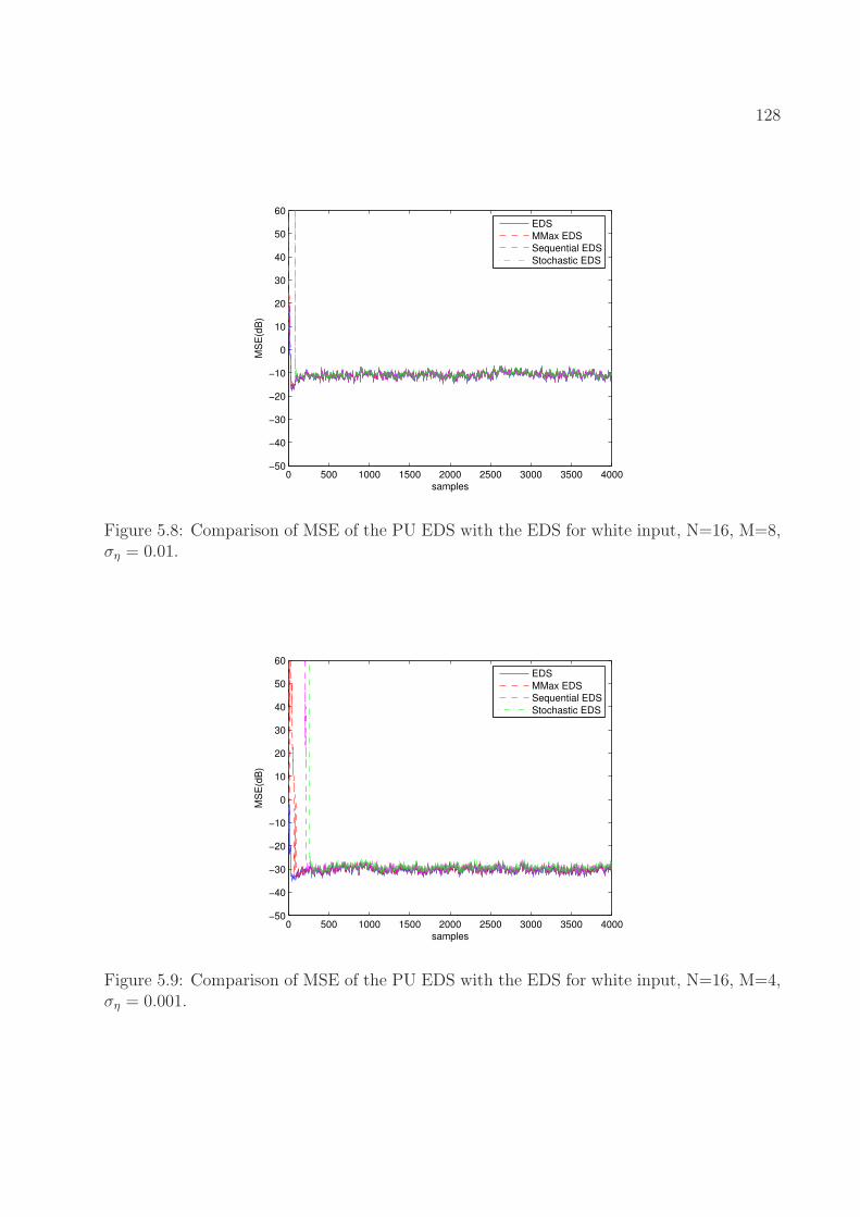
128

0 500 1000 1500 2000 2500 3000 3500 4000−50

−40

−30

−20

−10

0

10

20

30

40

50

60

samples

MS

E(d

B)

EDS

MMax EDS

Sequential EDS

Stochastic EDS


0 500 1000 1500 2000 2500 3000 3500 4000−50

−40

−30

−20

−10

0

10

20

30

40

50

60

samples

MS

E(d

B)

EDS

MMax EDS

Sequential EDS

Stochastic EDS


129

0 500 1000 1500 2000 2500 3000 3500 4000−50

−40

−30

−20

−10

0

10

20

30

40

50

60

samples

MS

E(d

B)

EDS

MMax EDS

Sequential EDS

Stochastic EDS


Table 5.5: The simulated MSE and theoretical MSE of the PU EDS in a time-varying systemfor white input and process noise ση = 0.001.


EDS (N=16) -29.9657 -30.4766MMax EDS (M=8) -29.9571 -30.4699

Sequential EDS (M=8) -29.7107 -30.3654Stochastic EDS (M=8) -29.6381 -30.3650MMax EDS (M=4) -30.2689 -30.4349

Sequential EDS (M=4) -29.3666 -29.9289Stochastic EDS (M=4) -29.2707 -29.9384

130

Table 5.6: The simulated MSE and theoretical MSE of the PU EDS in a time-varying systemfor white input and process noise ση = 0.01.


EDS (N=16) -10.7191 -11.0287MMax EDS (M=8) -10.6829 -11.0286

Sequential EDS (M=8) -10.4600 -11.0273Stochastic EDS (M=8) -10.4281 -11.0274MMax EDS (M=4) -10.5673 -11.0282

Sequential EDS (M=4) -9.7506 -11.0221Stochastic EDS (M=4) -9.6415 -11.0222

Tracking Performance Comparison of the MMax EDS with the EDS, RLS, MMax

RLS, CG, and MMax CG

The tracking performance of the MMax EDS is also compared with the full-update EDS, full-

update RLS, MMax RLS, full-update CG, and MMax CG. The same system identification

model is used. After 2000 samples/iterations pass, the unknown system in (4.57) is changed

by multiplying all coefficients by -1. Fig. 5.11 and Fig. 5.12 show the MSE results among

the EDS, MMax EDS, RLS, MMax RLS, CG, and MMax CG when M = 8 and M = 4,

respectively. White input is used. The results show that these algorithms have a similar

convergence rate after the unknown system is changed. It is also shown that the MMax

EDS, MMax RLS, and MMax CG with M = 4 can have a similar convergence rate to the

MMax EDS, MMax RLS, and MMax CG with M = 8 after the unknown system is changed.

The partial update length only affects the convergence rate at the beginning in this case.

This is because Q(n) gives a less reliable estimation of Q at the beginning when partial

update length decreases. The EDS and MMax EDS have convergence rates very close to

the full update RLS. The SORTLINE sorting method is used for MMax EDS, MMax RLS,

and MMax CG. The total number of multiplications of MMax EDS, MMax RLS, MMax CG

are N2 + 2NM + N + 2M , 2N2 + 2NM + 3N + M + 1, and 2N2 + M2 + 9N + M + 3 ,

131

0 500 1000 1500 2000 2500 3000 3500 4000−50

−40

−30

−20

−10

0

10

20

30

samples

MS

E(d

B)

EDS

MMax EDS M=8

CG

MMax CG M=8

RLS

MMax RLS M=8

Figure 5.11: Comparison of MSE of the MMax EDS with the EDS, RLS, MMax RLS, CG,and MMax CG for white input, N=16, M=8.

respectively. In this case, the full update length N is 16. The partial update length M is 8

and 4, respectively. The detailed computational complexities of these algorithms are shown

in Table 5.7. Overall, the EDS algorithms need fewer multiplications than the RLS and CG.

The results show that the MMax EDS with M=4 can achieve similar tracking performance

to the full-update EDS and RLS while reducing the computational complexity significantly.

5.7 Conclusion

In this chapter, different PU EDS algorithms are developed. Theoretical mean and mean-

square performance are derived for both time-invariant and time-varying systems. The

performance of different PU EDS algorithms is compared by using computer simulations.

The simulated results match the theoretical results. We can conclude that the PU EDS can

achieve a similar steady-state MSE as the full-update EDS while reducing the computational

complexity significantly. Among different PU EDS algorithms, the MMax EDS has the best

132

0 500 1000 1500 2000 2500 3000 3500 4000−50

−40

−30

−20

−10

0

10

20

30

samples

MS

E(d

B)

EDS

MMax EDS M=4

CG

MMax CG M=4

RLS

MMax RLS M=4

Figure 5.12: Comparison of MSE of the MMax EDS with the EDS, RLS, MMax RLS, CG,and MMax CG for white input, N=16, M=4.

Table 5.7: The computational complexities of the EDS, MMax EDS, RLS, MMax RLS, CG,and MMax CG.

Algorithms Number of Number ofmultiplications comparisonsper symbol per symbol

EDS (N=16) 816 –MMax EDS (M=8) 544 10MMax EDS (M=4) 408 10

RLS (N=16) 3721 –MMax RLS (M=8) 825 10MMax RLS (M=4) 693 10

CG (N=16) 3003 –MMax CG(M=8) 731 10MMax CG (M=4) 679 10

133

performance. The MMax EDS has a convergence rate close to the full-update EDS. The

performance of the PU EDS is also compared with the PU RLS and PU CG by using MMax

method. The MMax EDS can perform better than the MMax RLS and MMax CG, while

having a lower computational complexity. The MMax EDS has a faster convergence rate

than the MMax RLS and MMax CG. The MMax EDS, RLS, and CG can achieve the same

steady-state MSE.

Chapter 6

Deficient-Length RLS and EDS

The deficient-length adaptive filter addresses the situation when the length of the estimated

filter is less than the true length of the unknown filter. For a deficient-length adaptive filter,

let the filter length be M < N . The corresponding adaptive coefficients and the input

data vector are w(n− 1) = [w1(n− 1), w2(n− 1), ..., wM (n− 1)]T , and x(n) = [x(n), x(n−

1), ..., x(n −M + 1)]T . We can write the coefficients of the unknown system and the input

data as two parts

woN =

wo

wo

, xN(n) =

x(n)

x(n)

, (6.1)

where wo = [wo1, w

o2, ..., w

oM ]T , wo = [wo

M+1, woM+2, ..., w

oN ]

T , and x(n) = [x(n −M), x(n −

M − 1), ..., x(n−N + 1)]T . An M × 1 coefficient error vector is introduced as

z(n) = w(n)−wo. (6.2)

134

135

From (6.1), (2.1) can be rewritten as

d(n) = xT (n)wo + xT (n)wo + v(n), (6.3)

From (6.3) and (6.2), the above output error (2.3) can be written as

e(n) = xT (n)wo − xT (n)z(n− 1) + v(n). (6.4)

To determine the steady-state behaviors of the deficient-length RLS and EDS, two assump-

tions are needed.

Assumption I: The coefficient error z(n) is independent of the input signal x(n) in steady

state.

Assumption II: Noise v(n) is independent of the input signal x(n) and has zero mean.

6.1 Performance Analysis of Deficient-Length RLS

The RLS algorithm updates its coefficients according to the following recursion [43]:

P(0) = δ−1I, (6.5)

P(n) = λ−1[P(n− 1)− λ−1P(n− 1)x(n)xT (n)P(n− 1)

1 + λ−1xT (n)P(n− 1)x(n)], (6.6)

w(n) = w(n− 1) +P(n)x(n)e(n), (6.7)

where I is the identity matrix, P(n) is the gain matrix andP−1(n) = λn+1δI+∑n

i=1 λn−ix(i)xT (i).

δ−1 is an initial value. λ is the forgetting factor.

136

From (6.2), (6.4), and (6.7), the coefficient error can be expressed as

z(n) = z(n− 1)−P(n)x(n)xT (n)z(n− 1)

+ P(n)x(n)xT (n)wo +P(n)x(n)v(n). (6.8)

In [21], another LMS stochastic difference equation was derived by using the direct-averaging

method. Using the same method, equation (6.8) can be replaced by

z(n) = z(n− 1)− E{P(n)x(n)xT (n)}z(n− 1)

+ E{P(n)x(n)xT (n)}wo +P(n)x(n)v(n), (6.9)

as long as the gain matrix P(n) is small. To guarantee P(n) is small, a small initial δ−1

should be chosen.

6.1.1 Mean Performance

The mean behavior of the RLS coefficient error vector can be determined by taking the

expectation of both sides of (6.8) to yield

E{z(n)} = E{I−P(n)x(n)xT (n)}E{z(n− 1)}

+ E{P(n)x(n)xT (n)wo}, (6.10)

where we have used E{P(n)x(n)v(n)} = 0.

137

Multiplying both sides of (6.8) with P−1(n) yields

P−1(n)z(n) = P−1(n)z(n− 1)− x(n)xT (n)z(n− 1)

+ x(n)xT (n)wo + x(n)v(n). (6.11)

Taking the expectation and using Assumptions I, II, and also for steady state E{P−1(n)z(n)} =

E{P−1(n)z(n− 1)}, we get

E{x(n)xT (n)}E{z(∞)} = E{x(n)xT (n)wo}. (6.12)

Let the input data autocorrelation matrix R = E{x(n)xT (n)} and h = E{x(n)xT (n)wo}.

Then, the steady-state solution of (6.8) is

E{z(∞)} = R−1h. (6.13)

Therefore, the steady-state mean coefficient vector of the RLS adaptive filter is

E{w(∞)} = wo +R−1h, (6.14)

which means the steady-state coefficient vector of deficient-length RLS has a bias of R−1h.

For the sufficient length case, h = 0 since wo = 0, and the error vector in steady state is

equal to zero. For a white input signal, since x(n) and x(n) are uncorrelated, h = 0 and

E{w(∞)}white = wo. The deficient-length RLS adaptive filter converges in the mean.

138

6.1.2 Mean-Square Performance

We now determine the MSE performance of the deficient-length RLS algorithm. From (6.4),

the MSE ǫ(n) = E{e2(n)} can be expressed as the same equation (14) in [34],

ǫ(n) = ǫNmin + w∗TRN−Mwo − 2hT (n)E{z(n− 1)}

+ tr(RE{z(n− 1)zT (n− 1)}), (6.15)

where ǫNmin = E{v2(n)} is the variance of the input noise, and RN−M = E{x(n)xT (n)} is

the deficient-length (N −M) × (N −M) input data autocorrelation matrix. Uncorrelated

input can be used here. The excess mean-square error is given by

ǫex(n) = w∗TRN−Mwo − 2hT (n)E{z(n− 1)}

+ tr(RE{z(n− 1)zT (n− 1)}). (6.16)

Define the weight-error autocorrelation matrix K(n) = E{z(n)zT (n)}. Using Assumptions

I, II, and (6.9), K(n) is determined as follows:

K(n) = K(n− 1)−K(n− 1)F(n)

− FT (n)K(n− 1) + FT (n)K(n− 1)F(n)

+ DT (n)E{zT (n− 1)}+ E{z(n− 1)}D(n)

− DT (n)E{zT (n− 1)}F(n)− FT (n)E{z(n− 1)}D(n)

+ DT (n)D(n) + ǫNminE{P(n)x(n)xT (n)PT (n)}, (6.17)

where F(n) = E{x(n)xT (n)PT (n)}, and D(n) = w∗TE{x(n)xT (n)PT (n)}.

139

For the white noise input case, R = σ2xI, and we get

ǫ(n) = ǫNmin + σ2x||wo||2 + σ2

xtr(K(n− 1)), (6.18)

which is the same as equation (21) in [34]. Here (6.17) can still be used. Since x(n) and

x(n) are uncorrelated, D(n) in (6.17) is 0. K(n) is reduced to:

K(n) = K(n− 1)−K(n− 1)F(n)− FT (n)K(n− 1)

+ FT (n)K(n− 1)F(n) + ǫNminE{P(n)x(n)xT (n)PT (n)}, (6.19)

In this case, F(n) = ασ2xI, where α is a scalar. The proof is as follows by using mathematical

induction:

P(0) = δ−1I,

P(1) = λ−1δ−1I− β1λ−2δ−2x(1)xT (1),

P(2) = λ−2δ−1I− β1λ−3δ−2x(1)xT (1)− β2λ

−3δ−2x(2)xT (2)

+ 2β2β1λ−4δ−3x(2)xT (2)x(1)xT (1)

− β2β21λ

−5δ−4x(1)xT (1)x(2)xT (2)x(1)xT (1)

= λ−2δ−1I− β2λ−3δ−2x(2)xT (2)

− (β1λ−3δ−2 + γ1β2β

21λ

−5δ−4)x(1)xT (1)

+ 2γ2β2β1λ−4δ−3x(2)xT (1). (6.20)

Note the denominator of (6.6) is just a scalar, therefore the symbol β is used to represent

the denominators in the above equations. xT (i)x(j) is also a scalar, so symbol γ is also used.

140

From the above equations, we can induce that

P(n) = α1I−n∑

i=1

n∑

j=1

βijx(i)xT (j). (6.21)

To prove that (6.21) is true, we need to prove

P(n+ 1) = α11I−n+1∑

i=1

n+1∑

j=1

βi1j1x(i)xT (j). (6.22)

Suppose (6.21) is true,

P(n+ 1) = λ−1α1I− λ−1

n∑

i=1

n∑

j=1

βijx(i)xT (j)− λ−1(α2

1x(n)xT (n)

− 2n∑

i=1

n∑

j=1

βijx(i)xT (j)x(n+ 1)xT (n+ 1)

+n∑

i=1

n∑

j=1

n∑

i1=1

n∑

j1=1

βijβi2j2x(i)xT (j)

x(n+ 1)xT (n+ 1)x(i1)xT (j1))

= λ−1α1I− γ1

n+1∑

i=1

n+1∑

j=1

βijx(i)xT (j)

+ γ2

n∑

i=1

x(i)xT (n) + γ3

n∑

i=1

n∑

j1=1

x(i)xT (j1)

= α11I−n+1∑

i=1

n+1∑

j=1

βi1j1x(i)xT (j). (6.23)

Note that all xT (i)x(j) are scalars. All the symbols α, β, and γ represent scalars. So (6.21)

is proved.

141

Now consider x(n)xT (n)PT (n).

F(n) = x(n)xT (n)PT (n)

= x(n)xT (n)α1I−n∑

i=1

n∑

j=1

βijx(n)xT (n)x(i)xT (j)

= α1x(n)xT (n)−

n∑

j=1

βijx(n)xT (j). (6.24)

E{x(n)xT (n)PT (n)} = E{α1x(n)xT (n)} − E{

n∑

j=1

βijx(n)xT (j)}

= αE{x(n)xT (n)}

= ασ2xI. (6.25)

This result uses the property of white input, E{x(n)xT (j)} = 0 when j 6= n, since input is

zero-mean and each element is uncorrelated.

From (6.18) and (6.19), we see that the mean-square behavior of the white noise input is

independent of E{z(n− 1)}, which is not the same in the correlated input case.

6.1.3 Mean and Mean-Square Performance for Ergodic Input Sig-

nal

Assumption III: The input signal vector x(n) is ergodic in the autocorrelation function [22].

This indicates that R ≈ 1nQ(n) for n > M [22].

The time-varying optimal solution of the RLS algorithm [5] is

w(n) = Q−1(n)r(n), n > M (6.26)

142

where Q−1(n) = P(n), r(n) =∑n

i=1 λn−id(i)x(i), and M is the length of the deficient-length

filter. The following analysis is based on assuming the exponential weighting factor λ is

unity and ignoring the effects of initialization [22].

Substituting d(i) in r(n), we get

r(n) =n∑

i=1

x(i)xT (i)wo

+n∑

i=1

x(i)xT (i)wo +n∑

i=1

x(i)v(i)

= Q(n)wo + Q(n)wo +n∑

i=1

x(i)v(i), (6.27)

where Q(n) =∑n

i=1 x(i)xT (i).

Equation (6.26) becomes

w(n) = Q−1(n)(Q(n)wo + Q(n)wo +n∑

i=1

x(i)v(i))

= wo +Q−1(n)Q(n)wo +Q−1(n)n∑

i=1

x(i)v(i). (6.28)

The mean convergence is derived by taking the expectation of (6.28) as

w(n) = wo +Q−1(n)Q(n)wo

= wo + (nR)−1nRwo

= wo +R−1E{x(i)xT (i)}wo

= wo +R−1h, n > M, (6.29)

where R = E{x(i)xT (i)} ≈ 1nQ(n). This result is exactly the same as (6.14).

143

The weight error vector then becomes

z(n) = Q−1(n)Q(n)wo +Q−1(n)n∑

i=1

x(i)v(i). (6.30)

Using Assumptions I-III and (6.30), the weight-error autocorrelation matrix becomes

K(n) = E{Q−1(n)Q(n)wow∗T QT (n)Q−T (n)}

+ E{Q−1(n)n∑

i=1

n∑

j=1

x(i)xT (j)}E{v(i)v(j)}

= E{Q−1(n)Q(n)wow∗T QT (n)Q−T (n)}

+ ǫNminE{Q−1(n)Q(n)Q−1(n)}

= E{Q−1(n)Q(n)wow∗T QT (n)Q−T (n)}+ ǫNminE{Q−1(n)}

= R−1Rwow∗T RTR−T +1

nǫNminR

−1, n > M. (6.31)

Note that E{v(i)v(j)} = ǫNmin when i = j, otherwise it is zero.

The mean-square deviation [22] for deficient-length RLS is

De(n) = E{zT (n)z(n)} = tr{K(n)}

= tr{R−1Rwow∗T RTR−T}+ 1

nǫNmintr{R−1}

=M∑

i=1

1

λ2i

N−M∑

j=1

λ2jw

∗T wo +1

nǫNmin

M∑

i=1

1

λi

, n > M, (6.32)

where λi and λi are the eigenvalues of the correlation matrices R and R respectively.

144

The fourth term in (6.15) becomes

tr{RK(n)} = tr{Rwow∗T RTR−T}+ 1

nǫNmintr{I}

=M∑

i=1

1

λi

N−M∑

j=1

λ2jw

∗T wo +M

nǫNmin, n > M. (6.33)

Therefore, the MSE at steady state is finally

ǫ(n) = ǫNmin + w∗TRN−Mwo − 2hT (n)R−1h(n)

+M∑

i=1

1

λi

N−M∑

j=1

λ2jw

∗T wo +M

nǫNmin. (6.34)

6.2 Performance Analysis of Deficient-Length EDS

The EDS algorithm updates its coefficients according to the following recursion [5]:

w(n) = w(n− 1) + αg, (6.35)

α = −gT (Q(n)w(n− 1)− r(n))

gTQ(n)g, (6.36)

Q(n) =n∑

i=1

λn−ix(i)xT (i), (6.37)

r(n) =n∑

i=1

λn−id(i)x(i), (6.38)

where theM×1 vector g is the search direction at iteration n, which is taken to be “Euclidean

directions.” It is defined as gi = [0, · · · , 0, 1, 0, · · · , 0]T , where the 1 appears in the i-th

position. At each iteration n, the entire weight vector w(n) is updated by cycling through

all the Euclidean directions gi, i = 1, 2, · · · ,M [57].

145

Subtracting wo from both sides of (6.35), we have

z(n) = z(n− 1)− gT (Q(n)w(n− 1)− r(n))g

gTQ(n)g. (6.39)

Now consider the term Q(n)w(n− 1)− r(n). Since Q(n) = λQ(n− 1) + x(n)xT (n), r(n) =

λr(n− 1) + d(n)x(n), and from (2.1), (6.2), we get

Q(n)w(n− 1)− r(n)

= (λQ(n− 1) + x(n)xT (n))w(n− 1)

− (λr(n− 1) + d(n)x(n))

= λ(Q(n− 1)w(n− 1)− r(n− 1))

+ x(n)xT (n)w(n− 1)

− x(n)xT (n)wo − x(n)xT (n)wo − xv(n)

= λ(Q(n− 1)w(n− 1)− r(n− 1))

+ x(n)xT (n)z(n− 1)− x(n)xT (n)wo − x(n)v(n). (6.40)

Since Q(n− 1) = λQ(n− 2) + x(n− 1)xT (n− 1), r(n− 1) = λr(n− 2) + d(n− 1)x(n− 1),

d(n− 1) = xTN(n− 1)wo

N + v(n− 1), and so on, we can rewrite Q(n)w(n− 1)− r(n) as

Q(n)w(n− 1)− r(n) = (n∑

i=1

λn−ix(i)xT (i))z(n− 1)

− (n∑

i=1

λn−ix(i)xT (i))wo −n∑

i=1

λn−iv(i)x(i)

= Q(n)z(n− 1)−B(n)wo −C(n), (6.41)

where B(n) =∑n

i=1 λn−ix(i)xT (i), C(n) =

∑n

i=1 λn−iv(i)x(i).

146

Now we can rewrite the EDS coefficient error recursion in (6.39) as

z(n) = z(n− 1)− gT (Q(n)z(n− 1)−B(n)wo −C(n))g

gTQ(n)g. (6.42)

Using the direct-averaging method, (6.42) can be replaced by

z(n) = z(n− 1)− E{ggTQ(n)

gTQ(n)g}z(n− 1)− E{gg

TB(n)

gTQ(n)g}wo − ggTC(n)

gTQ(n)g. (6.43)

6.2.1 Mean Performance

The mean behavior of the EDS coefficient error vector can be determined by taking the

expectation of both sides of (6.42), which is different from the method used in [57]:

E{z(n)} = E{z(n− 1)} − E{ggTQ(n)

gTQ(n)g}E{z(n− 1)} − E{gg

TB(n)wo

gTQ(n)g}, (6.44)

where we have used E{ggTC(n)gTQ(n)g

} = 0.

Multiplying gTQ(n)g to both sides of (6.42) and taking the expectation gives

E{z(n)gTQ(n)g} = E{z(n− 1)gTQ(n)g} − E{gTQ(n)z(n− 1)g}

− E{gTB(n)wog}+ E{gTC(n)g}. (6.45)

Note that: (1) for steady state E{z(n)gTQ(n)g} = E{z(n− 1)gTQ(n)g}, (2) g and gT are

just the directions, and (3) E{C(n)} = 0. These give

E{Q(n)z(n− 1)} − E{B(n)wo} = 0. (6.46)

147

For steady state,

E{Q(n− 1)z(n− 1)} − E{B(n− 1)wo} = 0 (6.47)

is also true. Subtracting the two equations gives

E{x(n)xT (n)z(∞)− x(n)xT (n)wo} = 0. (6.48)

Then, the steady-state mean solution of the deficient-length EDS is the same as the deficient-

length RLS in (6.13). The steady-state mean coefficient vector of the EDS adaptive filter is

still (6.14). The deficient-length EDS adaptive filter also converges in the mean.

6.2.2 Mean-Square Performance

We now examine the MSE performance of the deficient-length EDS algorithm. The MSE of

deficient-length EDS is given by (6.15) for correlated input. Using Assumptions I, II, and

(6.43), the weight-error autocorrelation matrix K(n) is determined as follows:

K(n) = K(n− 1)−K(n− 1)J(n)− JT (n)K(n− 1) + JT (n)K(n− 1)J(n)

+ E{z(n− 1)}S(n) + ST (n)E{zT (n− 1)} − JT (n)E{z(n− 1)}S(n)

− ST (n)E{zT (n− 1)}J(n) + ST (n)S(n) + E{ggTC(n)

gTQ(n)g

CT (n)ggT

gTQ(n)g}, (6.49)

148

where J(n) = E{QT (n)ggT

gTQ(n)g}, S(n) = w∗TE{BT (n)ggT

gTQ(n)g}. For the white noise input case, we

also have (6.18). Since S(n) = 0 in (6.49), K(n) is reduced to

K(n) = K(n− 1)−K(n− 1)J(n)− JT (n)K(n− 1) + JT (n)K(n− 1)J(n)

+ E{ggTC(n)

gTQ(n)g

CT (n)ggT

gTQ(n)g}, (6.50)

The mean-square behavior is completed by specifying the autocorrelation matrixK(n), which

was not done in [57]. The steady-state mean-square behavior of white noise input is inde-

pendent of E{z(n− 1)}.

6.3 Simulations

6.3.1 System Model

The system identification model is shown in Fig. 2.1 and is taken from [57]. In this exper-

iment, the same unknown system is used as in [34]. It is a 16-order FIR filter, i.e., N=16,

with the impulse response

woN = [0.01, 0.02,−0.04,−0.08, 0.15,−0.3, 0.45,

0.6, 0.6, 0.45,−0.3, 0.15,−0.08,−0.04, 0.02, 0.01]T .

In our experiments, a deficient-length filter was used with M=12. The variance of input

noise v(n) is ǫNmin = 0.0001.

149

6.3.2 Correlated Input

The same input of the system is used as in [57]. It has the following form

x(n) = 0.8x(n− 1) + η(n), (6.51)

where η(n) is a zero-mean white Gaussian noise with unit variance. The results are obtained

by averaging 200 independent runs.

Fig. 6.1 and Fig. 6.2 illustrate the mean behaviors of deficient-length RLS with different

initial conditions δ−1. The sixth and eighth coefficient errors were obtained from simulation

and from the theoretical expression in (6.10) with correlated input signals. From these

figures, the simulation results agree with the theoretical results in steady-state. In the

transient state, the errors in the figure match better with small initial condition than with

large initial condition. This result makes sense because Assumption I is true for steady state,

but not for converging state. Assumption I could be true for the converging state only when

the initial condition δ−1 is very small. This situation is comparable to the step size µ in the

LMS algorithm. In LMS, Assumption I is reasonable for a small µ [43].

Fig. 6.3 and Fig. 6.4 illustrate the mean-square behaviors of deficient-length RLS with

different initial conditions δ−1. The theoretical expressions are (3.47) and (6.17). In steady

state, the simulation MSE agrees with the theoretical results.

Fig. 6.5 and Fig. 6.6 illustrate the mean and mean-square behaviors of deficient-length EDS.

The theoretical expressions are (6.44), (6.15), and (6.49). In steady state, the simulation

results agree with the theoretical results.

150

0 200 400 600 800 1000 1200−0.8

−0.6

−0.4

−0.2

0

0.2

0.4

0.6

iteration number

EZ

6(n

),E

Z8(n

)

Simulation

Theory

6th coeff error

8th coeff error

Figure 6.1: Comparison of theoretical and simulation curves of the mean behavior of the 6thand 8th coefficient errors of the deficient-length RLS for correlated input, and N=16, M=12,λ = 0.99, δ−1 = 0.1.

0 100 200 300 400−0.8

−0.6

−0.4

−0.2

0

0.2

0.4

0.6

iteration number

EZ

6(n

),E

Z8(n

)

Simulation

Theory

6th coeff error

8th coeff error

Figure 6.2: Comparison of theoretical and simulation curves of the mean behavior of the 6thand 8th coefficient errors of the deficient-length RLS for correlated input, and N=16, M=12,λ = 0.99, δ−1 = 100.

151

0 200 400 600 800 1000 1200−50

−40

−30

−20

−10

0

10

20

iteration number

MS

E(d

B)

Simulation

Theory

Figure 6.3: Comparison of theoretical and simulation curves of the mean-square behavior ofthe deficient-length RLS for correlated input, and N=16, M=12, λ = 0.99, δ−1 = 0.1.

0 100 200 300 400−50

−40

−30

−20

−10

0

10

20

iteration number

MS

E(d

B)

Simulation

Theory

Figure 6.4: Comparison of theoretical and simulation curves of the mean-square behavior ofthe deficient-length RLS for correlated input, and N=16, M=12, λ = 0.99, δ−1 = 100.

152

0 100 200 300 400

−0.6

−0.4

−0.2

0

0.2

iteration number

EZ

6(n

),E

Z8(n

)

Simulation

Theory

8th coeff error

6th coeff error

Figure 6.5: Comparison of theoretical and simulation curves of the mean behavior of the 6thand 8th coefficient errors of the deficient-length EDS for correlated input, and N=16, M=12,λ = 0.99.

0 100 200 300 400−60

−40

−20

0

20

40

60

iteration number

MS

E(d

B)

Simulation

Theory

Figure 6.6: Comparison of theoretical and simulation curves of the mean-square behavior ofthe deficient-length EDS for correlated input, and N=16, M=12, λ = 0.99.

153

0 200 400 600 800 1000 1200−0.6

−0.4

−0.2

0

0.2

0.4

iteration number

EZ

6(n

),E

Z8(n

)

Simulation

Theory

8th coeff error

6th coeff error

Figure 6.7: Comparison of theoretical and simulation curves of the mean behavior of the6th and 8th coefficient errors of the deficient-length RLS for white input, and N=16, M=12,λ = 0.99, δ−1 = 0.1.

6.3.3 White Input

In this experiment, the same unknown system is used, but the input signals are white. Fig.

6.7 and Fig. 6.8 illustrate the mean and mean-square behaviors of the deficient-length RLS.

Fig. 6.9 and Fig. 6.10 illustrate the mean and mean-square behaviors of the deficient-length

EDS.

6.3.4 Channel Equalization

Equalization performance is also examined between RLS and deficient-length RLS and be-

tween EDS and deficient-length EDS.

First, we use a simple short FIR channel [43]

C(z) = 0.5 + 1.2z−1 + 1.5z−2 − z−3. (6.52)

154

0 200 400 600 800 1000 1200−50

−40

−30

−20

−10

0

10

iteration number

MS

E(d

B)

Simulation

Theory

Figure 6.8: Comparison of theoretical and simulation curves of the mean-square behavior ofthe deficient-length RLS for white input, and N=16, M=12, λ = 0.99, δ−1 = 0.1.

0 100 200 300 400

−0.6

−0.4

−0.2

0

0.2

iteration number

EZ

6(n

),E

Z8(n

)

Simulation

Theory

6th coeff error

8th coeff error

Figure 6.9: Comparison of theoretical and simulation curves of the mean behavior of the6th and 8th coefficient errors of the deficient-length EDS for white input, and N=16, M=12,λ = 0.99.

155

0 100 200 300 400−60

−40

−20

0

20

40

60

iteration number

MS

E(d

B)

Simulation

Theory

Figure 6.10: Comparison of theoretical and simulation curves of the mean-square behaviorof the deficient-length EDS for white input, and N=16, M=12,λ = 0.99.

We assume the sufficient length of the equalizer is 35 and let the deficient length be 15. The

input sequence is 4-QAM. The results are obtained by averaging 50 independent runs. Fig.

6.11 and Fig. 6.12 illustrate the symbol-error-rate (SER) in log-scale between sufficient-

length and deficient-length equalizers for RLS and EDS. The SER is larger in the deficient-

length equalizer when SNR is small. When the signal-to-noise ratio (SNR) is greater than

13, the SER becomes the same for sufficient-length and deficient-length equalizers and goes

to zero. Since the deficient-length filter can get acceptable results, we can use the deficient-

length filter to reduce computational complexity. Compared with the SER of the MMax

RLS and EDS, the deficient-length RLS and EDS do not perform as well as the MMax RLS

and EDS. The MMax RLS and EDS can have similar SER as the full-update RLS and EDS.

Second, we use a complex channel with spectral nulls [43]. Its frequency response and impulse

response are shown in Fig. 6.13. We assume the sufficient length of the equalizer to be 75

and let the deficient length be 35. Fig. 6.14 shows the frequency and impulse responses

of the sufficient-length RLS equalizer and of the convolution of the channel and equalizer.

156

5 6 7 8 9 10 11 12 1310

−6

10−5

10−4

10−3

10−2

10−1

SNR(dB)

SE

R

Deficient RLS

RLS

Figure 6.11: Comparison of SER between RLS and deficient-length RLS.

Fig. 6.15 shows the responses of the deficient-length RLS. The results illustrate that the

deficient-length RLS does not perform as well as the sufficient RLS, but the results are still

acceptable. The EDS also has similar performance and the results are omitted.

6.4 Conclusion

Steady-state mean and mean-square error performance of the deficient-length RLS and EDS

are analyzed. We have shown that the deficient-length RLS and EDS converge in the mean

to the optimal Wiener solution [57]. In addition, we have derived expressions for the mean-

square error of deficient-length RLS and EDS. Simulation results agree with the derived

theoretical expressions. The performance of deficient-length RLS and EDS get worse when

a shorter length is used. Compared with the PU RLS and EDS, the deficient-length RLS

and EDS do not perform as well as the PU RLS and EDS.

157

5 6 7 8 9 10 11 12 1310

−6

10−5

10−4

10−3

10−2

10−1

SNR(dB)

SE

R

Deficient EDS

EDS

Figure 6.12: Comparison of SER between EDS and deficient-length EDS.

0 1 2 3−60

−50

−40

−30

−20

−10

0

ω (rad/sample)

dB

10 20 30

−0.5

0

0.5

index

Am

plit

ude

Figure 6.13: The frequency magnitude (left) and impulse (right) responses of the channel.

158

0 1 2 3

0

10

20

30

RLS equalizer

ω

dB

0 1 2 3

−20

−10

0

combination

ω

dB

20 40 60−4

−2

0

2

4

index

Am

plit

ud

e

20 40 60 80 1000

0.2

0.4

0.6

0.8

index

Am

plit

ud

e

Figure 6.14: The frequency magnitude responses of the RLS equalizer (left) and of theconvolution of the channel and the equalizer (right).

0 1 2 3

0

10

20

Deficient RLS equalizer

ω

dB

0 1 2 3

−40

−30

−20

−10

0

combination

ω

dB

10 20 30

−2

0

2

4

index

Am

plit

ud

e

20 40 60

0

0.2

0.4

0.6

0.8

index

Am

plit

ud

e

Figure 6.15: The frequency magnitude responses of the deficient-length RLS equalizer (left)and of the convolution of the channel and the equalizer (right).

Chapter 7

Special Applications of

Partial-Update Adaptive Filters

In this chapter, two special applications of PU adaptive filters are shown. One application is

using PU adaptive filters to detect Global System for Mobile Communication (GSM) signals

in a local GSM system using OpenBTS and Asterisk PBX. The other application is using

PU adaptive filters to do image compression in a system combining hyperspectral image

compression and classification.

7.1 PU Adaptive Filters in Detecting GSM signals in

a local GSM system using OpenBTS and Asterisk

PBX

A traditional GSM network is shown in Fig. 7.1 [33]. Mobile stations (MS) are connected

to base transceiver stations (BTS) through a wireless air interface. Base transceiver stations

159

160

are controlled by a basestation controller (BSC). The BTS reaches to a service provider’s

operating system through the base station controller (BSC) and switching subsystem. The

switching subsystem, mobile switch center/visitor location register (MSC/VLR), is responsi-

ble for connecting voice calls and routing the Short Message Service (SMS). For commercial

services, the service provider’s system authenticates the mobile stations with a shared key

(Ki) and an international mobile subscriber identity (IMSI) at the initial stage of mobile

connection. For the GSM (global system for mobile communications) MS, the Ki and the

IMSI information is stored in a subscriber identity module (SIM) card. During the initial

connection, a random key is created and used for the rest of the communication.

Figure 7.1: Traditional GSM network.

Nowadays, the Open Base Transceiver Station (OpenBTS) and Asterisk Private Branch

Exchange (PBX) are widely used for building a local GSM network for non-commercial

purposes. OpenBTS is an open source software-based GSM access point. It is used to

present a GSM air interface to GSM handsets. The OpenBTS acts like the traditional GSM

operator network infrastructure BTS. Asterisk software PBX is a software implementation

of a telephone private branch exchange (PBX) and it is used to connect calls as a MSC/VLR

via Session Initiation Protocol (SIP) and Voice-over-IP (VoIP). Fig. 7.2 shows a local GSM

161

system using OpenBTS and Asterisk PBX. Instead of building the complex infrastructure of

a traditional GSM network, the local GSM system using OpenBTS and Asterisk PBX only

needs a computer with a Linux system and a Universal Software Radio Peripheral (USRP).

OpenBTS and Asterisk are installed in a computer as normal software. The USRP is a

hardware device for software radio, which can transmit and receive signals under the control

of a computer and software such as GNU Radio and OpenBTS. The system controls local

cellular communications. GSM cellphones can call each other, send SMS to each other, or

call any SIP soft phone. The OpenBTS reads the IMSI of the MS and creates a virtual

SIP including the IMSI. This virtual SIP represents a certain GSM phone. It attempts to

register with Asterisk as a SIP soft phone. Once it succeeds registering with Asterisk and is

provided a phone number (extension), the GSM phone can be reached by dialing that phone

number [15]. Fig. 7.3 shows the functional block diagram of the local GSM system using

OpenBTS, Asterisk, two USRPs, and a computer. Since there are existing commercial GSM

BTS signals, a scanner is used to detect GSM signals to avoid conflicts with other GSM

BTS signals. The scanner uses the first USRP, and goes through each channel (200 kHz

bandwidth) in the PCS band (1930 - 1990 MHz). A detection algorithm is used to decide

if there is a GSM signal. After all the GSM signals are founded in the PCS band, our BTS

uses the second USRP, and it is set up by using a channel (frequency) different from the

detected signals.

The basic idea of the detection algorithm [50] in the scanner is that an adaptive line enhancer

is used to detect a frequency correction burst (FCB). A FCB is a complex sine wave with

frequency 67.7033 kHz. It is generated by modulating all zero bits with Gaussian minimum

shift keying (GMSK). The FCB is used to do the synchronization in a GSM system and it is

usually stronger than the normal burst. Using the adaptive line enhancer, we can separate

narrow band sinusoid signals from noise or wideband signals. Since the FCB is a sinusoid,

162

Figure 7.2: GSM network using OpenBTS and Asterisk PBX.

the periodicity is very high, and it is easier to be predicted by using an adaptive line enhancer

than the normal burst. Fig. 7.4 shows the diagram of an adaptive line enhancer. The input

signal is x(n), and a delay version of the input signal passes through an adaptive filter w(n).

The output of the adaptive filter is y(n). If the input signal is a sinusoid with some noise,

then the output should be a pure sinusoid and the error between them should be very small.

Adaptive filter algorithms NLMS and EDS can be used in the adaptive line enhancer. To

reduce the computational complexity, the partial update NLMS and EDS are also used.

The partial update NLMS algorithm in an adaptive filter system is summarized as:

e(n) = d(n)− xH(n)w(n), (7.1)

w(n+ 1) = w(n) + µe∗(n)x(n)

‖x(n)‖2, (7.2)

where µ is the step size.

In our simulation, the PCS band (1930-1990MHz) is scanned. It has 300 channels. The

NLMS, PU NLMS, EDS, and PU EDS can obtain the same results when detecting GSM

signals. The scanner using any of the adaptive filter algorithms can find the GSM signals

163

Figure 7.3: Functional-block description of local GSM system.

at channel 739 (1975.6 MHz), channel 742 (1976.2 MHz), channel 796 (1987.0 MHz), and

channel 804 (1988.6 MHz). Since a complex signal is used, the number of multiplications

of NLMS is 6N + 2 per sample, and the number of multiplications of PU NLMS is 6M + 2

per sample. The number of multiplications of EDS is 10N2 + 10N per sample, and the

number of multiplications of PU EDS is 6N2 + 4NM + 6N + 4M per sample. Note that

computational complexity of the error e(n) = d(n)−xH(n)w(n) is not calculated for the LMS

algorithm. Table 7.1 shows the comparison of computational complexity among full-update

NLMS, periodic NLMS, sequential NLMS, full-update EDS, periodic EDS, and sequential

EDS. The overall number of multiplications is represented in million (M). Since the GSM

signals in the PCS band are scanned, there are total of 300 channels. We also scan 6 times

for each channel to make sure the FCB can be caught. There are 10000 data samples for

each channel. We can see that the PU NLMS and PU EDS can reduce the overall number of

multiplications significantly. Table 7.2 shows the overall executed time by using C language

and a Linux system computer with CPU frequency 2GHz. We can see that the PU adaptive

filters can save overall executed time, especially for the PU EDS algorithm. If a real-time

164

Figure 7.4: Diagram of adaptive line enhancer.

processor with lower CPU frequency is used, the PU algorithms should be able to save more

execution time.

Table 7.1: The computational complexities of the LMS, periodic LMS, sequential LMS, EDS,periodic EDS, and sequential EDS

Algorithms Number of multiplications Overall number ofper sample multiplications

LMS(N=16) 98 1764Mperiodic LMS (L=2) 98 882Msequential LMS (N=8) 50 900M

EDS (N=16) 2720 48,960Mperiodic EDS (L=2) 2720 24,480Msequential EDS (N=8) 2176 39,168M

7.2 PU Adaptive Filters in a System Combining Hy-

perspectral Image Compression and Classification

A hyperspectral image contains information collected from across the electromagnetic spec-

trum. Spectral imaging divides the spectrum into hundreds of images/bands over a contin-

165

Table 7.2: Execution time using C and Linux

Algorithms Time (s)LMS(N=16) 9.50

periodic LMS (L=2) 6.11sequential LMS (N=8) 6.01

EDS (N=16) 211periodic EDS (L=2) 123sequential EDS (N=8) 161

uous spectral range. It is a three-dimensional data cube which has spatial domains (bands)

and a spectral domain. A typical hyperspectral image is shown in Fig. 7.5 [27]. It can be

used to discriminate the spectral features of minerals, soil, rocks, and vegetation [20]. It

has been widely used in space and earth science because of its rich information about the

compositional properties of surface materials. Spectral imaging applications are also used in

other areas including ecology, surveillance, historical manuscript research, agriculture, etc.

Classification and compression are common operations used in image processing. Image

classification is used to find special features of an image. It is usually performed on the

original image, not on the image after the compression and decompression process. Be-

cause of large storage volume and spectral and spatial sample data redundancy [44], it is

economical to compress hyperspectral images before transmitting, storing, and classifying

them. Basic compression methods for hyperspectral imagery are transform coding based

algorithms [47, 39, 16], Vector Quantization (VQ) based algorithms [42, 37], Differential

Pulse Code Modulation (DPCM) [52], and Adaptive Differential Pulse Code Modulation

(ADPCM) [31].

Compression and classification algorithms are conventionally performed independent of each

other and performed sequentially. However, some class distinctions may be lost after a

minimum distortion compression. There are very few compression/feature extraction meth-

ods which directly take classification goals (accuracy) into account in the way of feedback.

166

Figure 7.5: A typical hyperspectral image.

Usually, compression/feature extraction is performed - with no regard to the classification

objectives - before classification is performed. One of the few algorithms that accomplishes a

joint optimization of feature extraction and classification is a recent iterative neural learning

algorithm, called Generalized Relevance Learning Vector Quantization (GRLVQ) [23], which

produces impressive results for hyperspectral data in a version further modified to specifi-

cally address high-dimensional issues [35]. In GRLVQ, classification and feature extraction

are welded together with a 2-way feedback loop, and classification cannot be separated and

substituted by a different classifier. In this work, we propose a scheme that combines com-

pression and classification for the hyperspectral image. The optimal compressor is chosen

according to the classification results. In this scheme, the ADPCM method is used for

the compression. To reduce computational complexity, partial update (PU) adaptive filter

algorithms are also used in ADPCM for the compression of hyperspectral images. The clas-

sification algorithm is the SOM-hybrid artificial neural network (ANN) (SOM-ANN). Unlike

167

the GRLVQ, the compression method and classification method can be replaced by other

methods.

A system combining hyperspectral image compression and classification is shown in Fig.

7.6. The basic idea of this system is to implement classification on both the original un-

compressed image and the image after compression and decompression operations. The

classification error between pre- and post-compression is fed back to the compression sys-

tem in order to improve the compression system according to the optimization algorithm.

In this process, the quality of classification will gradually increase, and the compression

scheme will gradually improve, in order to capture important classification features. In this

scheme, compression is achieved by ADPCM, which has an adaptive predictor filter and a

quantizer. The filter algorithms in ADPCM are designed to minimize the mean-square or

least-square cost functions. Other compression algorithms can also be used in this scheme.

In this work, the ADPCM algorithm is chosen because the predictor filter can minimize

the error metric, the predictor filter has different parameters to be adjusted according to the

optimization algorithm, and different predictor filter algorithms can be chosen. By adjusting

different parameters or choosing different predictor filter algorithms, the ADPCM algorithm

can introduce flexibility into the compression and classification results. The cost function is

the classification error between the uncompressed image and the compressed-decompressed

image.

The optimal ADPCM predictor algorithm is chosen according to the best classification re-

sults. Different adaptive filtering algorithms for the ADPCM predictor are used in the

compression system, including Least Mean Square (LMS) and Euclidean Direction Search

(EDS). LMS is a very popular adaptive filtering algorithm. It has a low computational com-

plexity but has relatively slow convergence speed and high mean-square error (MSE). The

EDS algorithm has faster convergence speed and lower MSE than the LMS.

168

Figure 7.6: System combining compression and classification.

Since hyperspectral images usually have hundreds of bands and a large computer storage

size, the computational complexity of compression algorithms is a big consideration. To

further reduce the computational complexity, the PU LMS and PU EDS are also used for

the ADPCM predictor. The partial update method aims to reduce the computational cost

of the adaptive filters. Instead of updating all the N × 1 coefficients, it usually only updates

M × 1 coefficients, where M < N . Two different PU methods are used. One is the periodic

method, which can reduce the overall computational complexity by updating the filter coeffi-

cients periodically. The other method is stochastic PU, which can reduce the computational

complexity of each sample by randomly updating parts of the filter coefficients.

The quantizer in the ADPCM is the Jayant quantizer [5]. It is an adaptive quantizer and is

used to further reduce the quantization error. One-dimensional compression is applied along

the spectral domain. The compression is not applied to the 2-dimensional spatial domains,

nor to the 3-dimensional spectral and spatial domains, in order to avoid corruption of the

spectra, which can be detrimental for classification accuracy. Classification of a hyperspectral

169

image uses spectral pixels/vectors (each pixel/vector contains hundreds of bands) to do the

training, therefore keeping spectra uncorrupted is more important. If a 3-bit Jayant quantizer

was used, the LMS was used for the predictor algorithm, and the SOM-ANN algorithm was

used for classification; the classification accuracy of compression along spatial domains was

69.1%, while the classification accuracy of compression along the spectral domain was 77.3%.

The compression along the spectral domain increases around 8% in classification accuracy.

The classification algorithm is the SOM-hybrid artificial neural network (ANN) architecture

(SOM-ANN). It is a feed forward ANN with a self-organizing map (SOM) as a hidden layer,

and a categorization learning output layer coupled to it with a Widrow-Hoff learning rule.

Details are given in [36, 51, 26]. In an unsupervised phase, the SOM layer first forms its view

of the data clusters, which greatly assists the accurate learning of classes in a subsequent

supervised phase. The dual nature of the network also allows for the discovery of new

clusters and diagnosis of learning problems in the SOM. This ANN has proved to produce

both classification and clustering with great sensitivity to subtle but consistent spectral

differences, and consequently, to discriminate among large numbers of material classes with

high accuracy [36, 51, 26]. In this work, an improved method to implement the SOM-ANN

classification algorithm is used for better statistic results. The detail for this will be shown

in the section on simulations. Although we use the ADPCM method for the compression

and the SOM-ANN method for classification in this work, this scheme is not limited to the

ADPCM and SOM-ANN. Other compression methods and classification methods can also

be used in this scheme with proper modification.

170

Figure 7.7: One image band of the LCVF scene, obtained at 1.02987 µm.

7.2.1 Simulations

The hyperspectral image we use is the Lunar Crater Volcanic Field (LCVF), taken by the

AVIRIS sensor in 1994. The size of this image is 420 ×614 pixels ×194 bands. Details

of this scene and of the 23 surface cover classes used in this study are given in [36, 51],

which also show classification maps. One image band, at 1.02987 µm, is shown in Fig. 7.7.

The whole data cube is shown in Fig. 7.8. We use this image because of the availability

of previous classifications for comparison, and because we have the requisite number of

labeled test samples, ≥100 samples per class (exclusive of the labeled training samples) to

perform statistically meaningful evaluation of the classification accuracy on test data. A

few of the very small classes which do not have a total of 100 samples, are exceptions.

Atmospheric correction and removal of excessively noisy bands leave 194 bands, and the

resulting image is the source for our processing. We name this image LCVF-UNCOMP.

The SOM-ANN network classified LCVF-UNCOMP into 23 classes with ∼ 90% overall (or

weighted) accuracy (89.9% overall, κ = 89.23).

171

Figure 7.8: Hyperspectral image of the LCVF scene.

The comparison of classification accuracies among different predictor algorithms is shown

in Table 7.3. They are also compared with the uncompressed image (LCVF-UNCOMP).

The signal-to-noise ratio (SNR) is defined as the ratio of the power of the uncompressed

image over the power of the error between the decompressed image and the uncompressed

image. The SNR is somehow related to the classification accuracy. However, high SNR

does not necessarily indicate high classification accuracy. The ADPCM predictor algorithms

include LMS, periodic LMS, stochastic LMS, EDS, periodic EDS, and stochastic EDS. The

periodic algorithms have a period of 4. The stochastic algorithms have a PU length of 2.

The filter coefficients have a length of 8. The quantizer is the Jayant quantizer with 3 bits.

AVIRIS data is represented by 12 bits per pixel/spectral channel in the original distribution.

Therefore, the compression ratio is 4 : 1. The main purpose of using ADPCM compression,

rather than using a lossless compression method, is because it can adjust different parameters

or use different predictor filter algorithms, and therefore it can introduce flexibility to the

compression and classification results. Introducing flexibility might yield better classification

172

Table 7.3: The comparison of classification accuracies among different predictor algorithms

Algorithms Average of Averages of class accuracies SNR Number of Overallclass accuracies, averaged over 3 jack-knives. (dB) multiplications number of

from single Phase II (“clean training per-pixel multiplicationsexperiment. and test sample sets”) per-bandPhase I (%) Mean ± Std (%)

LCVF- 86.1 93.1 ± 0.46 – –UNCOMP

EDS 69.7 81.40 ± 0.40 32.937 406 20,311,660,320Periodic 74.7 82.07 ± 0.64 32.9606 103.5 5,177,972,520EDS

Stochastic 71.8 81.47 ±0.75 32.967 102 5,102,929,440EDSLMS 77.3 78.37 ± 0.90 33.0656 34 1,700,976,480

Periodic 74.9 81.67 ± 2.11 30.1327 20.5 1,025,588,760LMS

Stochastic 67.9 79.80 ± 1.65 30.1407 24 1,200,689,280LMS

results than those of the uncompressed image. In this study, we are comparing average (or

un-weighted) accuracies (i.e., averages of class accuracies), in order to gain insight of how,

on average, the prediction accuracies of classes are affected by the compression.

Table 7.3 shows results from two sets of experiments that we label as “Phase I” and “Phase

II.” These designations mark an important but unintended difference, which is the following.

After the Phase I experiments, we discovered that the training and test samples used for

training the classifier and for assessing its performance, respectively, had an overlap. Al-

though this overlap was less than 10% of the entire labeled set of samples, we decided to

repeat all runs with the training and test samples properly separated (with no overlap). By

that time, our resources improved and we could also afford to perform 3-fold jack-knives for

better statistics of the classification results. This includes the variance of the classification

accuracies across the 3 runs, which provides a measure of reliability. We label these exper-

iments (with “clean training and test sample sets;” and 3-fold jack-kniving) “Phase II.” In

other words, Phase I means the average of class accuracies from a single experiment, and

Phase II means the average of class accuracies averaged over 3 jack-knife runs. In Phase I,

173

each classification was performed only once (for reasons of limited resources), hence no aver-

ages and variances are shown. Phase I and Phase II results, of course, cannot be compared

with each other. However, comparisons within phases are still valuable. The classification

accuracies of the uncompressed data are 86.1% for Phase I and 93.1 ± 0.46% for Phase II.

The number of multiplications are also shown for each adaptive algorithm.

From Table 7.3 we can see that the classification accuracies are higher in Phase II, and the

classification accuracy is not necessarily determined by the SNR. The LMS algorithm has

the highest classification accuracy among all the algorithms in Phase I. The periodic EDS

has the highest classification accuracy in Phase II. However, the periodic LMS and stochastic

LMS have the lowest computational complexity. In Phase II, we can also see that the PU

LMS and PU EDS algorithms have higher classification accuracy than the full-update LMS

and EDS. It is possible that the PU adaptive filter in ADPCM can perform better than the

full-update adaptive-filter while reducing the computational complexity significantly. For

example, the EDS algorithm has 81.40 ± 0.40% classification accuracy in Phase II and its

total number of multiplications for the whole data set is 20,311,660,320, while the periodic

EDS algorithm has 82.07 ± 0.64% classification accuracy in Phase II and its total number

of multiplications is 5,177,972,520. Note that the number of multiplications in the table is

a per-pixel per-band number. To calculate the total number of multiplications, a constant

number 420 × 614 × 194 = 50, 028, 720, which is the number of spatial image pixels times

the number of image bands, needs to be multiplied by the per-pixel per-band number of

multiplications. From Table 7.3 we can see that the SNR of the LMS is higher than the SNR

of the periodic LMS and stochastic LMS, however the classification accuracy of the LMS is

lower than that of the periodic LMS and stochastic LMS in Phase II. This shows that high

SNR does not necessarily indicate high classification accuracy.

Moreover, the classification accuracy of each class is different when using different predictor

174

algorithms. Table 7.4 shows details of the Phase II classification error for each class when

using different predictor algorithms. The results were obtained by averaging three jack-

knife runs. The classification error of each class is defined by the number of misclassified

samples over the total number of each class. The rows in red represent the classes with high

classification errors, include classes F, I, M, V, and W. These classes are classes with few

training samples and/or classes with high spectral variance. They are easily misclassified

into similar classes because small differences are lost by applying the compression operation.

By using different predictor filter algorithms in the ADPCM compression algorithm, it can

introduce flexibility to the compression and classification results. For this LCVF data set, the

periodic EDS gives the highest average classification accuracy. The periodic LMS gives the

lowest classification error for classes F and I. The periodic EDS gives the lowest classification

error for classes M and V. The stochastic EDS gives the lowest classification error for class

W.

175

Table 7.4: The classification error, in units of (% misclassified samples)/100, of each classby using different predictor algorithms

Class EDS periodic EDS stochastic EDS LMS periodic LMS stochastic LMSA 0.045977 0.070115 0.041379 0.041379 0.033333 0.088506B 0.241176 0.150980 0.170588 0.211765 0.127451 0.137255C 0.105159 0.138889 0.121032 0.073413 0.158730 0.115079D 0.016260 0.040650 0.058072 0.042973 0.029036 0.022067E 0.055331 0.044534 0.041835 0.028340 0.052632 0.022942F 0.500000 0.520833 0.541667 0.531250 0.406250 0.500000G 0.242424 0.291667 0.208333 0.250000 0.246212 0.287879H 0.207937 0.214286 0.334920 0.315873 0.236508 0.207937I 0.508333 0.620833 0.545833 0.529167 0.483333 0.566667J 0.114286 0.079365 0.090476 0.050794 0.077778 0.071429K 0.156433 0.078947 0.093567 0.102339 0.097953 0.154971L 0.215100 0.272080 0.193732 0.286325 0.145299 0.440171M 0.456349 0.361111 0.466270 0.736111 0.591270 0.517857N 0.066138 0.035714 0.033069 0.058201 0.050264 0.048942O 0.109557 0.125874 0.111888 0.144522 0.165501 0.110723P 0.073935 0.066416 0.096491 0.090226 0.083960 0.060150Q 0.083333 0.060606 0.064394 0.113636 0.068182 0.034091R 0.075000 0.075000 0.041667 0.141667 0.108333 0.133333S 0.083333 0.069444 0.104167 0.076389 0.083333 0.097222T 0.044872 0.044872 0.076923 0.051282 0.051282 0.064103U 0.079365 0.057540 0.063492 0.115079 0.059524 0.043651V 0.458333 0.308333 0.433333 0.491667 0.375000 0.341667W 0.335378 0.404908 0.325153 0.494888 0.484663 0.576687

Chapter 8

Conclusion

8.1 Dissertation Summary

The work in this dissertation aims to apply basic partial-update methods to adaptive fil-

ter algorithms including CMA1-2, NCMA, LSCMA, EDS, and CG. A new PU method,

the selective-sequential method, is developed for LSCMA. The mathematical analysis of the

PU adaptive filter algorithm focuses on the convergence conditions, the steady-state perfor-

mance, and the tracking performance. The convergence performance of each PU adaptive

filter is shown by computer simulations. Detailed computational complexity has been cal-

culated for each partial update method. Performance is compared among different partial

update methods for each adaptive filter algorithm. Performance is also compared among

different adaptive filter algorithms. In most cases, the PU algorithms can achieve similar

performance to the full-update algorithms while reducing the computational complexity sig-

nificantly. The PU adaptive filters can achieve similar steady-state MSE as the full-update

filters. Among different PU methods, the MMax method usually has a convergence rate

very close to the full-update method. The sequential and stochastic methods usually con-

176

177

verge slower than the MMax method. However, the MMax method does not always perform

well with the LSCMA algorithm. The sequential LSCMA usually has the best performance

among the PU LSCMA algorithms. The PU LSCMA can achieve similar steady-state MSE

as the full-update LSCMA in tracking a time-varying system. The PU NCMA may perform

better than the full-update NCMA in tracking a time-varying system. The MMax EDS can

converge faster than the MMax RLS and CG. It can converge to the same steady-state MSE

as the MMax RLS and CG, while having a lower computational complexity. The PU LMS

and PU EDS can also perform a little better in a system combining hyperspectral image

compression and classification.

The major work includes:

1. Basic partial-update methods including periodic, sequential, stochastic, and MMax PU

methods, have been applied to adaptive filter algorithms including CMA1-2, NCMA,

LSCMA, EDS, and CG. A new PU method, the selective-sequential method, is devel-

oped for LSCMA.

2. The mathematical analyses including convergence conditions, steady-state performance,

and tracking performance have been derived for the PU adaptive filter algorithms.

3. Computer simulations with proper examples have been done to demonstrate the math-

ematical analysis and show the performance of PU adaptive filter algorithms. The

performance is compared between the original adaptive filter algorithms and different

partial-update methods. The convergence rate, steady-state performance, and tracking

performance have been compared for different PU methods.

4. Computational complexity has been calculated for each adaptive filter algorithm. It has

also been compared for each partial-update method. Numerical examples and proper

178

applications have been shown to illustrate how many additions and multiplications can

be saved by using PU methods.

5. Deficient-length adaptive filters including RLS and EDS have been studied. The math-

ematical analyses including the convergence conditions and the steady-state perfor-

mance have been shown. The performance of the deficient-length RLS and EDS have

been compared to the performance of PU RLS and PU EDS.

6. Besides applications of system identification and channel equalization, two special ap-

plications of using partial update adaptive filters are also presented. One application is

using PU adaptive filters to detect GSM signals in a local GSM system using OpenBTS

and Asterisk PBX. The other application is using PU adaptive filters to do image com-

pression in a system combining hyperspectral image compression and classification.

8.2 Future Work

This dissertation focuses on least-square adaptive filter algorithms such as LSCMA, EDS, and

CG. Although partial update methods can reduce the computational complexity significantly

for these algorithms, their computational costs are still high compared with steepest-descent

algorithms such as LMS, CMA1-2, and NCMA. In the future, new partial update methods

should be developed to further reduce the computational complexity of the least-square

algorithms. The PU methods should also be applied to adaptive filter algorithms which

have not been addressed in the literature or in this dissertation. In this dissertation, PU

adaptive filter algorithms have been shown to achieve similar performance to full-update

adaptive filter algorithms in most cases, but do not achieve better performance. In the

future, new partial update methods should be developed to achieve better performance than

full-update algorithms. New applications should also be explored to see if PU adaptive filters

179

can perform better than full-update adaptive filters.

Bibliography

[1] S. Attallah and S. W. Liaw, “Analysis of DCTLMS algorithm with a selective coefficient

updating,” IEEE Trans. Circuits and Systems II: Analog and Digital Signal Processing,

vol. 48, no. 6, pp. 628-632, June 2001.

[2] S. Attallah, “The wavelet transform-domain LMS adaptive filter with partial subband-

coefficient updating,” IEEE Trans. Circuits and Systems II: Express Briefs, vol. 53, no.

1, pp. 8-12, Jan. 2006.

[3] B. G. Agee, “The least-squares CMA: A new technique for rapid correction of con-

stant modulus signals,” in Proc. International Conference Acoustics, Speech, and Signal

Processing, Apr. 1986, vol. 11, pp. 953-956.

[4] B. G. Agee, “The property restoral approach to blind adaptive signal extraction,” PhD

dissertation, Department of Electrical Engineering and Computer Science, University of

California, Davis, CA, June, 1989.

[5] T. Bose, Digital Signal and Image Processing. New York: Wiley, 2004.

[6] A. Carini and G. L. Sicuranza, “Analysis of transient and steady-state behavior of a

multichannel filtered-x partial-error Affine Projection algorithm,” EURASIP Journal on

Audio, Speech, and Music Processing, vol. 2007 ID. 31314.

180

181

[7] P. S. Chang and A. N. Willson, “Analysis of conjugate gradient algorithms for adaptive

filtering,” IEEE Trans. Signal Processing, vol. 48, no. 2, pp. 409-418, Feb. 2000.

[8] G. Deng, “Partial update and sparse adaptive filters,” IET Signal Processing, vol. 1, no.

1, pp. 9-17, 2007.

[9] P. S. R. Diniz, G. O. Pinto, and A. Hjorungnes, “Data selective partial-update affine

projection algorithm,” in Proc. International Conference Acoustics, Speech, and Signal

Processing, Apr. 2008, pp. 3833-3836.

[10] K. Dogancay and O. Tanrikulu, “Normalised constant modulus algorithm with selec-

tive partial updates,” in Proc. International Conference Acoustics, Speech, and Signal

Processing, May 2001, vol. 4, pp. 2181-2184.

[11] K. Dogancay, Partial-Update Adaptive Signal Processing. Academic Press, 2008.

[12] S. C. Douglas, “Analysis and implementation of the max-NLMS adaptive filter,” in

Proc. Twenty-Ninth Asilomar Conference on Signals, Systems and Computers, 1995, vol.

1, pp. 659-663.

[13] S. C. Douglas, “Adaptive filters employing partial updates,” IEEE Trans. Circuits and

Systems II: Analog and Digital Signal Processing, vol. 44, no. 3, pp. 209-216, Mar. 1997.

[14] D. L. Duttweiler, “Proportionate normalized least-mean-squares adaptation in echo

cancelers,” IEEE Trans. Speech, and Audio Processing, vol. 8, no. 5, pp. 508-518, Sept.

2000.

[15] B. Ferguson, [Online]. “Communication between GSM devices and the PSTN via inte-

gration of Google Voice and OpenBTS with the Asterisk PBX,” 2011.

182

[16] J. E. Fowler and J. T. Rucker, “3D wavelet-based compression of hyperspectral im-

agery,” Hyperspectral Data Exploitation: Theory and Applications, C.-I. Chang, Ed., pp.

379-407, chapter 14, John Wiley & Sons, Hoboken, NJ, USA, 2007.

[17] H. Furukawa, Y. Kamio, and H. Sasaoka, “Co-channel interference reduction method

using CMA adaptive array antenna,” in Proc. 7th IEEE International Symposium Per-

sonal, Indoor, Mobile Radio Communications, Oct. 1996, vol. 2, pp. 512-516.

[18] D. N. Godard, “Self-recovering equalization and carrier tracking in two-dimensional

data communication systems,” IEEE Trans. Commun., vol. 28, no. 11, pp. 1867-1875,

Nov. 1980.

[19] M. Godavarti and A. O. Hero III, “Partial update LMS algorithms,” IEEE Trans.

Signal Processing, vol. 53, no. 7, pp. 2382-2399, 2005.

[20] R. O. Green, “Summaries of the 6th annual JPL airborne geoscience workshop,” in

Proc. AVIRIS Workshop, Mar. 1996, vol. 1.

[21] S. Haykin, Adaptive Filter Theory. 3th ed. New Jersey: Prentice-Hall, 1996.

[22] S. Haykin, Adaptive Filter Theory, 4th ed. New Jersey: Prentice Hall, 2002.

[23] B. Hammer, and Th. Villmann, “Generalized relevance learning vector quantization,”

Neural Networks, vol. 15, pp. 1059-1068, 2002.

[24] K. Hilal and P. Duhamel “A convergence study of the constant modulus algorithm

leading to a normalized-CMA and block-normalized-CMA,” in Proc. EUSIPCO, Aug.

1992, pp. 135-138.

[25] M. L. Honig, U. Madhow, and S. Verdu, “Blind adaptive interference suppression for

the near-far resistant CDMA,” in Proc. GLOBECOM, 1994, vol. 1, pp. 379-384.

183

[26] E. S. Howell, E. Merenyi, and L. A. Lebofsky, “Classification of asteroid spectra using

a neural network,” Geophysics Research, vol. 99, no. 10, pp. 847-865, 1994.

[27] [Online]. Available: http://rst.gsfc.nasa.gov/Intro/Part2 24.html

[28] C. R. Johnson, Jr., P. Schnitter, T. Endres, J. Behm, D. Brown and R. A. Casas, “Blind

equalization using the constant modulus criterion: A review,” Proc. IEEE, vol. 86, no.

10, pp. 1927-1950, Oct. 1998.

[29] A. W. H. Khong and P. A. Naylor, “Selective-tap adaptive filtering with performance

analysis for identification of time-varying systems,” IEEE Trans. Audio, Speech, and

Language Processing, vol. 15, no. 5, pp. 1681-1695, July 2007.

[30] A. W. H. Khong, P. A. Naylor, and J. Benesty, “A low delay and fast converging

improved proportionate algorithm for sparse system identification,” EURASIP Journal

on Audio, Speech, and Music Processing, vol. 2007, ID. 84376.

[31] M. Larsen, T. Bose, and A. Venkatachalam, “Hyperspectral image restoration and

coding,” in Proc. Thirty-Sixth Asilomar Conference on Signals, Systems and Computers,

Nov. 2002, vol.2, pp. 1740-1744.

[32] W. Lee, B. R. Vojcic, and R. L. Pickholtz, “Constant modulus algorithm for blind

multiuser detection,” in Proc. IEEE 4th International Symposium on Spread Spectrum

Techniques and Applications Proceedings, Sept. 1996, vo1. 3, pp. 1262-1266.

[33] A. Loula, [Online]. “OpenBTS Installation and Configuration Guide v0.1,” 2009.

[34] K. Mayyas, “Performance analysis of the deficient length LMS adaptive algorithm,”

IEEE Trans. Signal Processing, vol. 53, no. 8, pp. 2727-2734, Aug. 2005.

[35] M. J. Mendenhall, and E. Merenyi, “Relevance-based feature extraction for hyperspec-

tral images,” IEEE Trans. Neural Networks vol. 19, no. 4, pp 658-672, April 2008.

184

[36] E. Merenyi, W.H. Farrand, J.V. Taranik, and T.B. Minor, “Classification of hyperspec-

tral imagery with neural networks: comparison to conventional tools,” Machine Learning

Reports 04/2011 T. Villmann and F.-M. Schleif, Ed., vol. 5, no. 4, pp 1-15, April 2011,

ISSN:1865-3960 http://www.techfak.uni-bielefeld.de/fschleif/mlr/mlr 04 2011.pdf. Also

submitted to EURASIP Journal on Advances in Signal Processing, special issue on Neu-

ral Networks for Remotely Sensed Data Interpretation, 2011.

[37] G. Motta, F. Rizzo, and J. A. Storer, “Compression of hyperspectral imagery,” in Proc.

Data Compression Conference, Mar. 2003, pp. 25-27.

[38] P. A. Naylor and A. W. H. Khong, “Affine projection and recursive least squares

adaptive filters employing partial updates,” in Proc. Thirty-Eighth Asilomar Conference

on Signal, System & Computers, Nov. 2004, vol. 1, pp. 950-954.

[39] B. Penna, T. Tillo, E. Magli, and G. Olmo, “Transform coding techniques for lossy

hyperspectral data compression,”

IEEE Trans. Geosci. Remote Sens., vol. 45, no. 5, pp. 1408-1421, May 2007.

[40] M. R. Petraglia, and D. B. Haddad, “New adaptive algorithms for identification of sparse

impulse responses - Analysis and comparisons,” in Proc. ISWCS, 2010, pp. 384-388.

[41] [Online]. Available: http://www.calstatela.edu/centers/berp/docs/Wireless

Channel Models.pdf

[42] M. J. Ryan and J. F. Arnold, “The lossless compression of AVIRIS images by vector

quantization,” IEEE Trans. Geosci. Remote Sens., vol. 35, no. 3, May 1997.

[43] A. H. Sayed, Fundamentals of Adaptive Filtering. New York: Wiley, 2003.

[44] G. Shaw and D. Manolakis, “Signal processing for hyperspectral image exploitation,”

Signal Processing Mag., vol. 19, no. 1, Jan. 2002.

185

[45] A. Sugiyama, H. Sato, A. Hirano, and S. Ikeda, “A fast convergence algorithm for

adaptive FIR filters under computational constraint for adaptive tap-position control,”

IEEE Trans. Circuits and Systems II: Analog and Digital Signal Processing, vol. 43, no.

9, pp. 629-636, Sept. 1996.

[46] A. Sugiyama, S. Ikeda, and A. Hirano, “A fast convergence algorithm for sparse-tap

adaptive FIR filters identifying an unknown number of dispersive regions,” IEEE Trans.

Signal Processing, vol. 50, no. 12, pp. 3008-3017, Dec. 2002.

[47] X. Tang and W. A. Pearlman, “Lossy-to-lossless block-based compression of hyperspec-

tral volumetric data,” in Proc. IEEE Int. Conf. Image Process., 2004, pp. 3283-3286.

[48] J. R. Treichler and B. G. Agee, “A new approach to multipath correction of constant

modulus signals,” IEEE Trans. Acoustics, Speech, and Signal Processing, vol. 31, no. 2,

pp. 459-472, Apr. 1983.

[49] J. R. Treichler and M. G. Larimore, “The tone capture properties of CMA-based

interference suppressors,” IEEE Trans. Acoustics, Speech, and Signal Processing, vol.

33, no. 4, pp. 946-958, Aug. 1985.

[50] G. N. Varma, U. Sahu, and G. P. Charan, “Robust frequency burst detection algorithm

for GSM/GRPS,” in Proc. IEEE Vehicular Technology Conference, Sept. 2004, vol. 6,

pp. 3843-3846.

[51] T. Villmann, E. Merenyi, and B. Hammer, “Neural maps in remote sensing image

analysis,” Neural Networks, vol. 16, pp. 389-403, 2003.

[52] H. Wang and K. Sayood, “Lossless predictive compression of hyperspectral images,”

Hyperspectral Data Compression, pp. 35-56. Springer, 2006.

186

[53] S. Werner, J. A. Apolinario, Jr., and P. S. R. Diniz, “Set-membership proportionate

Affine Projection algorithms,” EURASIP Journal on Audio, Speech, and Music Process-

ing, vol. 2007, ID. 34242.

[54] J. Wu, M. Doroslovacki, “A mean Convergence analysis for partial update NLMS

algorithms,” in Proc. CISS, Mar. 2007, pp. 31-34.

[55] G. F. Xu and T. Bose, “Analysis of the Euclidean direction search adaptive algorithm,”

in Proc. International Conference on Acoustics, Speech and Signal Processing, pp. 1689-

1692, Apr. 1998.

[56] G. F. Xu, “Fast algorithms for digital filtering: Theory and applications,” Ph.D.

dissertation, University of Colorado, 1999.

[57] Z. K. Zhang, T. Bose, L. Xiao, and R. Thamvichai, “Performance analysis of the

deficient length EDS adaptive algorithms,” in Proc. APCCAS, Dec. 2006, pp. 222-226.

partialupdateadaptivefiltering...partialupdateadaptivefiltering bei xie abstract adaptive ﬁlters...

Documents