particle astrophysics theory group department of physics · arxiv:hep-ph/9803479v2 18 dec 1998...
TRANSCRIPT

arX
iv:h
ep-p
h/98
0347
9v2
18
Dec
199
8
Electroweak baryogenesis
Mark Trodden∗
Particle Astrophysics Theory Group
Department of Physics
Case Western Reserve University
10900 Euclid Avenue
Cleveland, OH 44106-7079.
Abstract
Contrary to naive cosmological expectations, all evidence suggests that the
universe contains an abundance of matter over antimatter. This article re-
views the currently popular scenario in which testable physics, present in
the standard model of electroweak interactions and its modest extensions,
is responsible for this fundamental cosmological datum. A pedagogical ex-
planation of the motivations and physics behind electroweak baryogenesis is
provided, and analytical approaches, numerical studies, up to date develop-
ments and open questions in the field are also discussed.
CWRU-P6-98 Submitted to Reviews of Modern Physics
Typeset in REVTEX
1

Contents
I Introduction 4
II Baryon Number Violation in the Electroweak Theory 9
A Zero temperature results . . . . . . . . . . . . . . . . . . . . . . . . . . . 15
B Nonzero temperature results . . . . . . . . . . . . . . . . . . . . . . . . . 18
1 A Mechanical Analogy . . . . . . . . . . . . . . . . . . . . . . . . . . . 18
2 The Electroweak Theory . . . . . . . . . . . . . . . . . . . . . . . . . . 19
III C and CP Violation 24
A Standard Model CP Violation: the KM Matrix . . . . . . . . . . . . . . . 24
B The Two-Higgs Doublet Model . . . . . . . . . . . . . . . . . . . . . . . . 26
C CP Violation from Higher Dimension Operators . . . . . . . . . . . . . . . 27
D General Treatment . . . . . . . . . . . . . . . . . . . . . . . . . . . . . . . 29
IV The Electroweak Phase Transition 29
A The finite temperature effective potential . . . . . . . . . . . . . . . . . . 35
B Dimensional Reduction . . . . . . . . . . . . . . . . . . . . . . . . . . . . 40
C Numerical Simulations – Lattice Approaches . . . . . . . . . . . . . . . . 42
D Other Approaches . . . . . . . . . . . . . . . . . . . . . . . . . . . . . . . 44
E Subcritical fluctuations . . . . . . . . . . . . . . . . . . . . . . . . . . . . 46
F Erasure of the Baryon Asymmetry: Washout . . . . . . . . . . . . . . . . 47
G Summary . . . . . . . . . . . . . . . . . . . . . . . . . . . . . . . . . . . . 49
V Local Electroweak Baryogenesis 50
A Local Baryogenesis Through Unwinding . . . . . . . . . . . . . . . . . . . 51
B Kicking Configurations Across the Barrier . . . . . . . . . . . . . . . . . . 56
C Making Progress . . . . . . . . . . . . . . . . . . . . . . . . . . . . . . . . 61
2

VI Nonlocal Baryogenesis 62
A Thin Bubble Walls . . . . . . . . . . . . . . . . . . . . . . . . . . . . . . . 64
B Thick Bubble Walls . . . . . . . . . . . . . . . . . . . . . . . . . . . . . . 69
1 Spontaneous Baryogenesis . . . . . . . . . . . . . . . . . . . . . . . . . 69
2 Classical Force Baryogenesis . . . . . . . . . . . . . . . . . . . . . . . . 70
C Summary and Making Progress . . . . . . . . . . . . . . . . . . . . . . . . 72
VII A Realistic Model of EWBG: the MSSM 72
A The Electroweak Phase Transition in the MSSM . . . . . . . . . . . . . . 73
B Extra CP Violation in the MSSM . . . . . . . . . . . . . . . . . . . . . . 75
VIII Topological Defects and the Departure from Thermal Equilibrium 76
A Electroweak Symmetry restoration and the Baryogenesis Volume . . . . . 77
B Local Baryogenesis and Diffusion in Defects . . . . . . . . . . . . . . . . . 79
C A Specific Geometry and Examples . . . . . . . . . . . . . . . . . . . . . 82
D A Particle Physics Model . . . . . . . . . . . . . . . . . . . . . . . . . . . 84
E Summary . . . . . . . . . . . . . . . . . . . . . . . . . . . . . . . . . . . . 86
IX Concluding Remarks and Looking to the Future 86
3

I. INTRODUCTION
The most basic distinction drawn between particles found in nature is that between
particle and antiparticle. Since antiparticles were first predicted (Dirac, 1930; Dirac, 1931)
and observed (Anderson, 1932; Anderson, 1933), it has been clear that there is a high degree
of symmetry between particle and antiparticle. This means, among other things, that a world
composed of antimatter would behave in a similar manner to our world. This basic tenet
of particle physics, the symmetry between matter and antimatter, is in stark contradiction
to the wealth of everyday and cosmological evidence that the universe is composed almost
entirely of matter with little or no primordial antimatter.
The evidence that the universe is devoid of antimatter comes from a variety of different
observations. On the very small scale, the absence of proton-antiproton annihilations in our
everyday actions, constitutes strong evidence that our world is composed only of matter
and no antimatter. Moving up in scale, the success of satellite launches, lunar landings, and
planetary probes indicate that our solar system is made up of the same type of matter that we
are, and that there is negligible antimatter on that scale. To determine whether antimatter
exists in our galaxy, we turn to cosmic rays. Here we see the first detection of antimatter
outside particle accelerators. Mixed in with the many protons present in cosmic rays are a
few antiprotons, present at a level of around 10−4 in comparison with the number of protons
(see for example Ahlen et al. (1988)). However, this number of antiprotons is consistent with
their secondary production through accelerator-like processes, p+ p→ 3p+ p, as the cosmic
rays stream towards us. Thus there is no evidence for primordial antimatter in our galaxy.
Finally, if matter and antimatter galaxies were to coexist in clusters of galaxies, then we
would expect there to be a detectable background of γ-radiation from nucleon-antinucleon
annihilations within the clusters. This background is not observed and so we conclude that
there is negligible antimatter on the scale of clusters (For a review of the evidence for a
baryon asymmetry see Steigman (1976)).
A natural question to ask is, what is the largest scale on which we can say that there
4

is no antimatter? This question was addressed by Steigman (1976),and by Stecker (1985),
and in particular has been the subject of a careful recent analysis by Cohen et al. (1998).
If large domains of matter and antimatter exist, then annihilations would take place at the
interfaces between them. If the typical size of such a domain was small enough, then the
energy released by these annihilations would result in a diffuse γ-ray background and a
distortion of the cosmic microwave radiation, neither of which is observed. Quantitatively,
the result obtained by the latter authors is that we may safely conclude that the universe
consists entirely of matter on all scales up to the Hubble size. It therefore seems that the
universe is fundamentally matter-antimatter asymmetric.
The above observations put an experimental upper bound on the amount of antimatter in
the universe. However, strict quantitative estimates of the relative abundances of baryonic
matter and antimatter may also be obtained from the standard cosmology. Primordial
nucleosynthesis (for a review see Copi et al. (1995)) is one of the most powerful tools of the
standard cosmological model. The theory allows accurate predictions of the cosmological
abundances of all the light elements, H, 3He, 4He, D, B and 7Li, while requiring only a single
input parameter. Define nb to be the number density of baryons in the universe. Similarly
define nb to be the number density of antibaryons, and the difference between the two to be
nB. Then, if the entropy density in the universe is given by s, the single parameter required
by nucleosynthesis is the baryon to entropy ratio
η ≡ nBs
=nb − nb
s, (1)
and one may conservatively say that calculations of the primordial light element abundances
are correct if
1.5 × 10⁻¹⁰ < η < 7 × 10⁻¹⁰ . (2)
Although the range of η within which all light element abundances agree with observations
is quite narrow (see figure 1), its existence at all is remarkable, and constitutes a strong
confirmation of the standard cosmology. For recent progress in nucleosynthesis see Tytler
et al. (1996) and Hogan (1997).
5

The standard cosmological model provides a complete and accurate description of the
evolution of the universe from extremely early times (a few minutes) to the present day
(10− 20 billion years) given a host of initial conditions, one of which is the value of η. This
standard picture is based on classical, fluid sources for the Einstein equations of General
Relativity (GR). While the success of the standard cosmology is encouraging, there remains
the question of the initial conditions. One approach is just to consider the initial values of
cosmological parameters as given. However, the values required for many parameters are
extremely unnatural in the sense that the tiniest deviation from them leads to a universe
entirely different from the one that we observe. One well known example of this is the initial
value of the mass density of the universe, the naturalness of which is at the root of the
flatness problem of the standard cosmology.
The philosophy of modern cosmology, developed over the last thirty years, is to attempt
to explain the required initial conditions on the basis of quantum field theories of elementary
particles in the early universe. This approach has allowed us to push our understanding of
early universe cosmology back to much earlier times, conservatively as early as 10−10 seconds,
and perhaps much earlier.
The generation of the observed value of η in this context is referred to as baryogenesis.
A first step is to outline the necessary properties a particle physics theory must possess.
These conditions were first identified by Sakharov (1967) and are now referred to as the
three Sakharov Criteria. They are:
• Violation of the baryon number (B) symmetry.
• Violation of the discrete symmetries C (charge conjugation) and CP (the composition
of parity and C)
• A departure from thermal equilibrium.
The first of these is rather obvious. If no processes ever occur in which B is violated,
then the total number of baryons in the universe must remain constant, and therefore no
6

asymmetry can be generated from symmetric initial conditions. The second Sakharov cri-
terion is required because, if C and CP are exact symmetries, then one can prove that
the total rate for any process which produces an excess of baryons is equal to the rate of
the complementary process which produces an excess of antibaryons and so no net baryon
number can be created. That is to say that the thermal average of B, which is odd under
both C and CP , is zero unless those discrete symmetries are violated. Finally, there are
many ways to explain the third criterion. One way is to calculate the equilibrium average
of B:
〈B〉T = Tr(e−βHB)
= Tr[(CPT )(CPT )−1e−βHB)]
= Tr(e−βH(CPT )−1B(CPT )]
= −Tr(e−βHB) , (3)
where in the third step I have used the requirement that the Hamiltonian H commutes with
CPT , and in the last step used the properties of B that it is odd under C and even under P
and T symmetries. Thus 〈B〉T = 0 in equilibrium and there is no generation of net baryon
number. This may be loosely described in the following way. In quantum field theories in
thermal equilibrium, the number density of any particle species, X say, depends only on the
energy of that species, through
neq(X) =1
e(E−µ)/T ± 1, (4)
where µ is the chemical potential corresponding to baryon number. Since the masses of
particle and antiparticle are equal by virtue of the CPT theorem, and µ = 0 if baryon
number is violated, we have that
Neq(X) =∫
d3p
(2π)3neq = Neq(X) , (5)
and again there is no net asymmetry produced.
7

The focus of this article is to review one popular scenario for generating the baryon
asymmetry of the universe (BAU), as quantified in equation (2), within the context of
modern cosmology. In general, such scenarios involve calculating nB, and then dividing by
the entropy density
s =2π2
45g∗T
3 , (6)
where g∗ is the effective number of massless degrees of freedom at temperature T . While
there exist many attempts in the literature to explain the BAU (for a review see Dolgov
(1992)), I will concentrate on those scenarios which involve anomalous electroweak physics,
when the universe was at a temperature of 102 GeV (for earlier reviews see Turok (1992),
Cohen et al. (1993), and Rubakov and Shaposhnikov (1996)). The production of the BAU
through these models is referred to as electroweak baryogenesis.
In the next section I will describe baryon number violation in the electroweak theory
both at zero and at nonzero temperature. In section III I shall move on to the subject of CP
violation, explaining how this arises in the standard model and how it is achieved in some
popular extensions. Section IV contains an account of the electroweak phase transition,
including a discussion of both analytic and numerical approaches. Having set up the frame-
work for electroweak baryogenesis, I turn in section V to the dynamics in the case where
baryon production occurs close to a phase boundary during a phase transition. In section
VI, I then extend these ideas to include the effects of particle transport, or diffusion. Section
VII contains a description of how baryogenesis is implemented in a popular extension of the
standard model, the minimal supersymmetric standard model (MSSM). In section VIII, I
explain how, in some extensions of the electroweak theory, baryogenesis may be mediated by
topological defects, alleviating the constraints on the order of the phase transition. Finally,
in section IX I summarize the results and comment on open questions and future directions
in the field.
It is my hope that this article will fulfill its intended role as both a review of the back-
ground and basic material for beginners in the field, and as a summary of and commentary
8

on the most recent results and directions in the subject. However, the focus of this arti-
cle, as in any such endeavor, is quite idiosyncratic, and I apologize to any of my colleagues
whose work has been omitted or incorrectly detailed. A different focus can be found in other
accounts of the subject and, in particular, for a comprehensive modern review of numerical
approaches I recommend Rubakov and Shaposhnikov (1996).
A note about conventions. Throughout I use a metric with signature +2 and, unless
explicitly stated otherwise, I employ units such that h = c = k = 1 so that Newton’s
constant is related to the Planck mass through G = M−2pl .
II. BARYON NUMBER VIOLATION IN THE ELECTROWEAK THEORY
The standard model of unified electromagnetic and weak nuclear interactions (Glashow,
1961; Weinberg, 1967; Salam, 1968) is based on the gauge groups SU(2)×U(1). The model
is described by the Lagrangian density
L = (Dµφ)†Dµφ− 1
4FµνF
µν − 1
4W aµνW
aµν + V (φ) + Lf . (7)
Here, the field strengths are
Fµν = ∂µBν − ∂νBµ ,
W aµν = ∂µA
aν − ∂νA
aµ + gεabcAbµA
cν ,
where Bµ is the hypercharge gauge field and Aaµ are the weak isospin gauge fields. The
covariant derivative is
Dµ = ∂µ −i
2gτ.Aµ −
i
2g′Bµ ,
and the Higgs potential is
V (φ) =λ
4(φ†φ− v2)2 . (8)
In the above, g is the SU(2) coupling constant, g′ is the U(1) coupling constant, λ is the
Higgs self-coupling, and v = 246 GeV is the vacuum expectation value (VEV) of the Higgs.
9

The potential V (φ) is chosen so that the gauge symmetry is spontaneously broken down
to the U(1) of electromagnetism that is realized by the vacuum today, and Lf denotes the
fermionic sector of the theory that I will describe in a moment. Note that it is conventional
to define
αW ≡ g2
4π≃ 1
29, (9)
and to write the ratio of g′ to g as
tan θW ≡ g′
g, (10)
where the experimentally measured value of the weak mixing angle θW is given by
sin2 θW ≃ 0.23 . (11)
It will be useful to briefly describe a slightly different formulation of the SU(2)+Higgs
theory, equivalent to considering the purely bosonic part of the standard model and ignoring
the U(1) hypercharge gauge field. The Lagrangian may be written in the form
L = −1
2Tr(WµνW
µν) − 1
2Tr(DµΦ)†DµΦ − λ
4
[
Tr(Φ†Φ) − v2]2
. (12)
In this form, the standard Higgs doublet φ = (φ1, φ2) is related to the matrix Φ by
Φ(x, t) =
φ∗2 φ1
−φ∗1 φ2
. (13)
For reference, g = 0.65, the gauge boson mass is mW = 12gv and the Higgs boson mass is
mH =√
2λv. Note that
Φ†Φ = (ϕ∗1ϕ1 + ϕ∗
2ϕ2)
1 0
0 1
, (14)
so that one can write
Φ =σ√2U , (15)
where σ2 = 2 (ϕ∗1ϕ1 + ϕ∗
2ϕ2) = TrΦ†Φ, and U is an SU(2) valued field which is uniquely
defined at any spacetime point where σ does not vanish. Without loss of generality, impose
the condition that at all times
10

lim|x|→∞
σ(x, t) = v , (16)
lim|x|→∞
U(x, t) =
1 0
0 1
. (17)
In A0 = 0 gauge, a vacuum configuration is of the form
Φ =v√2U
Aj =1
ig∂jUU
† . (18)
At any time t when σ(x, t) 6= 0 for all x we have that U(x, t) is a map from R3 with the
points at infinity identified, that is S3, into SU(2) and therefore U(x, t) can be associated
with an integer-valued winding
NH(t) = w[U ] =1
24π2
∫
d3x ǫijkTr[U †∂iUU†∂jUU
†∂kU ] , (19)
the Higgs winding number. If Φ(x, t) evolves continuously in t then NH(t) can change only
at times when there is a zero of σ at some point in space. At such times, NH is not defined;
at all other times, it is integer-valued. Note that the Higgs winding number of a vacuum
configuration (18) is equal to its Chern-Simons number
NCS(t) ≡g2
32π2
∫
d3x ǫijkTr(
Ai∂jAk +2
3igAiAjAk
)
. (20)
However, for a general non-vacuum configuration the Chern-Simons number is not integer-
valued.
Finally, the fermionic sector of the full SU(2) × U(1) theory is described by
Lf = Ll + Lq , (21)
where the lepton and quark sector Lagrangians for a single family are:
Ll = −iΨγµDµΨ − ieRγµDµeR + h(eRφ
†Ψ + ΨφeR) (22)
11

Lq = − i(u, d)LγµDµ
u
d
L
− iuRγµDµuR − idRγ
µDµdR
−Gd
[
(u, d)L
φ+
φ
dR + dR(φ−, φ∗)
u
d
L
]
−Gu
[
(u, d)L
−φ∗
φ−
uR + uR(−φ, φ+)
u
d
L
]
, (23)
where I have written φ = (φ+, φ0), with φ− = (φ+)∗. Here, e is the electron, u and d are
the up and down quarks respectively and Ψ represents the left-handed lepton doublet. The
indices L and R refer to left- and right-handed components, and Gd and Gu are Yukawa
coupling constants.
When extended to three families, this contains the six types of quarks U i = (u, c, t),
Di = (d, s, b), the electron, muon and tau lepton, and their associated neutrinos. Note that
gauge invariant fermion mass terms are generated through couplings to the Higgs doublet
Φ.
At the classical level, the number of each fermionic species is separately conserved in
all processes. This is reflected in the fact that for each species there exists a global U(1)
current, which is exactly classically conserved. In the standard model there are a total of 12
different species and so there are 12 separate conserved global currents. In particular, for
baryons, one may write a vectorlike current
jµB =1
2QγµQ , (24)
where Q represents quarks, and there is an implied sum over the color and flavor indices.
Now, due to quantum effects, any axial current ψγµγ5ψ of a gauge coupled Dirac fermion ψ,
is anomalous (Adler, 1969; Bell and Jackiw, 1969). This is relevant to baryon number since
the electroweak fermions couple chirally to the gauge fields. If we write the baryon current
as
jµB =1
4
[
Qγµ(1 − γ5)Q+ Qγµ(1 + γ5)Q]
, (25)
only the axial part of this vector current is important when one calculates the divergence.
12

This effect can be seen by calculating triangle graphs (see figure 2) and leads to the following
expressions for the divergences of the baryon number and lepton number currents;
∂µjµB = ∂µj
µl = nf
(
g2
32π2W aµνW
aµν − g′2
32π2FµνF
µν
)
, (26)
where nf is the number of families,
W µν =1
2ǫµναβWαβ (27)
is the dual of the SU(2) field strength tensor, and an analogous expression holds for F
The anomaly is important because of the multiple vacuum structure of the theory (see
figure 3), as I will describe in the following subsections. Equation (26) may be written as
∂µjµB = ∂µj
µl = nf
(
g2
32π2∂µK
µ − g′2
32π2∂µk
µ
)
, (28)
where the gauge non-invariant currents are defined by
Kµ = ǫµναβ(
W aναA
aβ −
1
3gǫabcA
aνA
bαA
cβ
)
,
kµ = ǫµναβFναBβ . (29)
For simplicity, consider space to be a 3-sphere and consider the change in baryon number
from time t = 0 to some arbitrary final time t = tf . For transitions between vacua, the
average values of the field strengths are zero at the beginning and the end of the evolution.
Since the final term in (28) is strictly proportional to the field strength of the U(1) gauge
fields, we may ignore this term. Then, using (20), the change in baryon number may be
written as
∆B = ∆NCS ≡ nf [NCS(tf ) −NCS(0)] . (30)
Although the Chern-Simons number is not gauge invariant, the change ∆NCS is. Thus,
since NCS is integral (as we have mentioned), changes in Chern-Simons number result in
changes in baryon number which are integral multiples of the number of families nf .
To understand this structure more completely, since the U(1) gauge fields are unimpor-
tant here, I will return to the SU(2) theory. Consider fermion production in the background
13

of the evolving Higgs and gauge fields and ignore the back-reaction of the fermions on the
bosonic fields. Consider the dynamics of nonzero energy configurations with nonzero Higgs
winding. A simple example (Ambjørn et al., 1989) is
Φ(x) =v√2U[1](x)
Aµ(x) = 0 , (31)
where U[1](x) is a winding number one map, say,
U[1](x) = exp (iη(r)τ · x) , (32)
with η(0) = −π and η(∞) = 0. The configuration (31) has no potential energy but does carry
gradient energy because the covariant derivatives DiΦ do not vanish. This configuration has
NH = 1 (where NH is defined in (19)). If the configuration (31) were released from rest it
would radiate away its energy and relax towards a vacuum configuration. There are two
very different ways for this to occur (Turok and Zadrozny, 1990). If the characteristic size
of U[1] is large compared to m−1W , then the gauge field will evolve until it lines up with the
Higgs field making the covariant derivatives zero, and at late times NH will still be one. If
the characteristic size is small the configuration will shrink, the Higgs field σ will go through
a zero, and at late times NH will be zero. This dynamics is the subject of section V.
Note that NH is not invariant under large gauge transformations. However, the change
∆NH in Higgs winding is gauge invariant, and the two distinct relaxation processes are
distinguished by whether ∆NH is zero or nonzero. To be definite, I will always choose the
gauge such that the prototypical initial configuration is of the form (31) which has NH = 1.
Now, if the fields relax to the vacuum by changing the Higgs winding then there is no
anomalous fermion number production. However, if there is no net change in Higgs winding
during the evolution (for example σ never vanishes) then there is anomalous fermion number
production.
To understand these claims consider two sequences of configurations beginning with the
wound up configuration (31) and ending at the classical vacuum (18). The first sequence
14

ends at the vacuum (18) with U = 1 while the second ends up at U = U[1]. Note that
these sequences cannot be solutions to the classical equations of motion since the initial
configurations carry energy whereas the final ones do not. Throughout both sequences the
boundary conditions (16) and (17) are maintained. For the first sequence, σ must vanish at
some intermediate configuration since the Higgs winding changes. For the second sequence,
the change in Higgs winding is zero and σ need not vanish.
Now introduce an SU(2)L weak fermionic doublet, ψ. The fermion is given mass through
the usual gauge invariant coupling to the Higgs field Φ, and for simplicity assume that both
the up and down components of the doublet have the same mass m. The fermion field is
quantized in the background of the bosonic fields given by the above interpolation.
The anomaly equation (26) reduces here to
∂µJµ =
g2
32π2Tr(WW ) , (33)
which, when integrated, implies that the change in the fermion number from the beginning
to the end of a sequence is given by
∫
d3x J0∣
∣
∣
∣
final−∫
d3x J0∣
∣
∣
∣
initial= −w[U ] , (34)
where U is that of the final configuration (18). For the first sequence w is one, whereas for
the second it is zero. Thus fermion number is violated in processes for which the config-
uration (31) unwinds via gauge unwinding, but is not violated when such a configuration
unwinds via a Higgs unwinding.
A. Zero temperature results
We have seen that the vacuum of the electroweak theory is degenerate, labeled by NH
and NCS. The field theories constructed around these vacua are entirely equivalent and
may be obtained from one another through large gauge transformations. However, transi-
tions between these vacua result in the anomalous production of fermions via the anomaly
15

equation (26). Such transitions violate baryon number and so are classically forbidden since
baryon number is an exact global symmetry of the theory. In fact, as I shall describe, at zero
temperature, baryon number violating processes occur through quantum tunneling between
the classical vacua of the theory.
In the infinite dimensional gauge and Higgs field configuration space, adjacent vacua
of the electroweak theory are separated by a ridge of configurations with energies larger
than that of the vacuum (see figure 3) The lowest energy point on this ridge is a saddle
point solution (Dashen et al., 1974; Christ, 1980) to the equations of motion with a single
negative eigenvalue, and is referred to as the sphaleron (Manton, 1983; Klinkhamer and
Manton, 1984). The sphaleron plays a central role in the calculation of the rate of baryon
number violating processes.
The calculation of the tunneling rate between degenerate vacua in quantum field theories
is well-established (for a review see Coleman (1979)). One first constructs the Euclideanized
action SE, obtained from the Minkowski space action by performing a Wick rotation
t→ −it ≡ τ . (35)
In the case of pure gauge theories, one then finds the solution to the Euclidean equations of
motion which interpolates between the two vacuum states and minimizes the Euclidean ac-
tion. Such a solution to the full four-dimensional Euclidean system is known as an instanton
and may be seen as a time series of three-dimensional configurations. The transition rate
between the degenerate vacua is then proportional to
exp(−SE)|instanton . (36)
When the theory in question has a Higgs field, as in the electroweak theory, the cal-
culation of the tunneling amplitude is a little more complicated. In this case, there are
no nonzero size configurations that minimize the Euclidean action, and a slightly different
approach is used. The procedure is to fix the size of the Euclidean configurations in the
functional integral by explicitly introducing a constraint (Affleck, 1981a). The functional
16

integral is then evaluated using these constrained instantons and, finally, one performs an
integral over the instanton size.
As an estimate of the zero temperature B violating rate in the electroweak theory, I shall
follow the approach of ’t Hooft (1976). Consider the pure gauge SU(2) theory (note no Higgs
field). The relevant configurations are finite action solutions to the Euclidean equations of
motion. Further, as I described earlier, the configurations of interest must possess non-zero
gauge winding in order for baryon number violation to take place. If we consider the case in
which the instanton interpolates between adjacent vacua of the theory, then the topological
charge of such a solution is ∆NCS = 1. Now, the quantity
∫
d4x (W aµν − W a
µν)2 (37)
is positive semi-definite for any gauge field configuration. This allows us to construct a
bound on the Euclidean action of configurations in the following way. Expanding (37) gives
∫
d4x[
Tr(WµνWµν) + Tr(WµνW
µν) − 2Tr(WµνWµν)]
≥ 0 . (38)
Now, in terms of the Euclidean action and the Chern-Simons number, this may then be
written as
4SE − 2
(
16π2
g2
)
NCS ≥ 0 , (39)
which finally yields
SE ≥ 8π2
g2NCS . (40)
The NCS = 1 instanton saturates this bound, which means that the rate per unit volume of
baryon number violating processes at zero temperature is approximately
Γ(T = 0) ∼ exp(−2SE) ∼ 10−170 . (41)
This is so small that if the universe were always close to zero temperature, not one event
would have occurred within the present Hubble volume ever in the history of the universe.
17

B. Nonzero temperature results
We have seen that the rate of baryon number violating processes is negligible at zero
temperature. This is to be expected since such events occur through quantum tunneling
under a high potential barrier (∼ 10TeV). If this were the case at all temperatures, it is safe
to say that electroweak baryon number violation would have no observable consequences. In
this section we shall see that, when one includes the effects of nonzero temperature, classical
transitions between electroweak vacua become possible due to thermal activation.
1. A Mechanical Analogy
Let us begin with a warmup example. Consider an ideal pendulum of mass m and length
l, confined to rotate in the plane. the Lagrangian is
L =1
2ml2θ2 −mgl(1 − cos θ) . (42)
the system possesses a periodic vacuum structure labeled by integer n
θn = 2nπ . (43)
The Schrodinger equation describing the quantum mechanics of this system is
hω
2
(
−α d2
dχ2+
1
αsin2 χ
)
ψn(χ) = Enψn(χ) , (44)
where χ ≡ θ/2, ω ≡ g/l and α ≡ hω/(4mgl) ≪ 1. Since the potential is periodic in the
angle θ, the wave-functions will be periodic and therefore the multiple vacuum structure
of the system is manifest. However, if one performs perturbation theory, Taylor expanding
the potential about a chosen minimum (θ = 0) and keeping only the first term, then the
Schrodinger equation becomes that for a simple harmonic oscillator and all information
about the periodic vacua is lost. This situation is analogous to most familiar calculations
in the electroweak theory, in which perturbation theory is usually a safe tool to use. Such
an approximation scheme is only valid when the energy of the pendulum is much less than
18
the height of the barrier preventing transitions between vacua (c.f. the sphaleron). In that
limit, quantum tunneling between vacua is exponentially suppressed as expected. This may
be seen by employing a different approximation scheme which preserves periodicity – the
semiclassical (WKB) approximation.
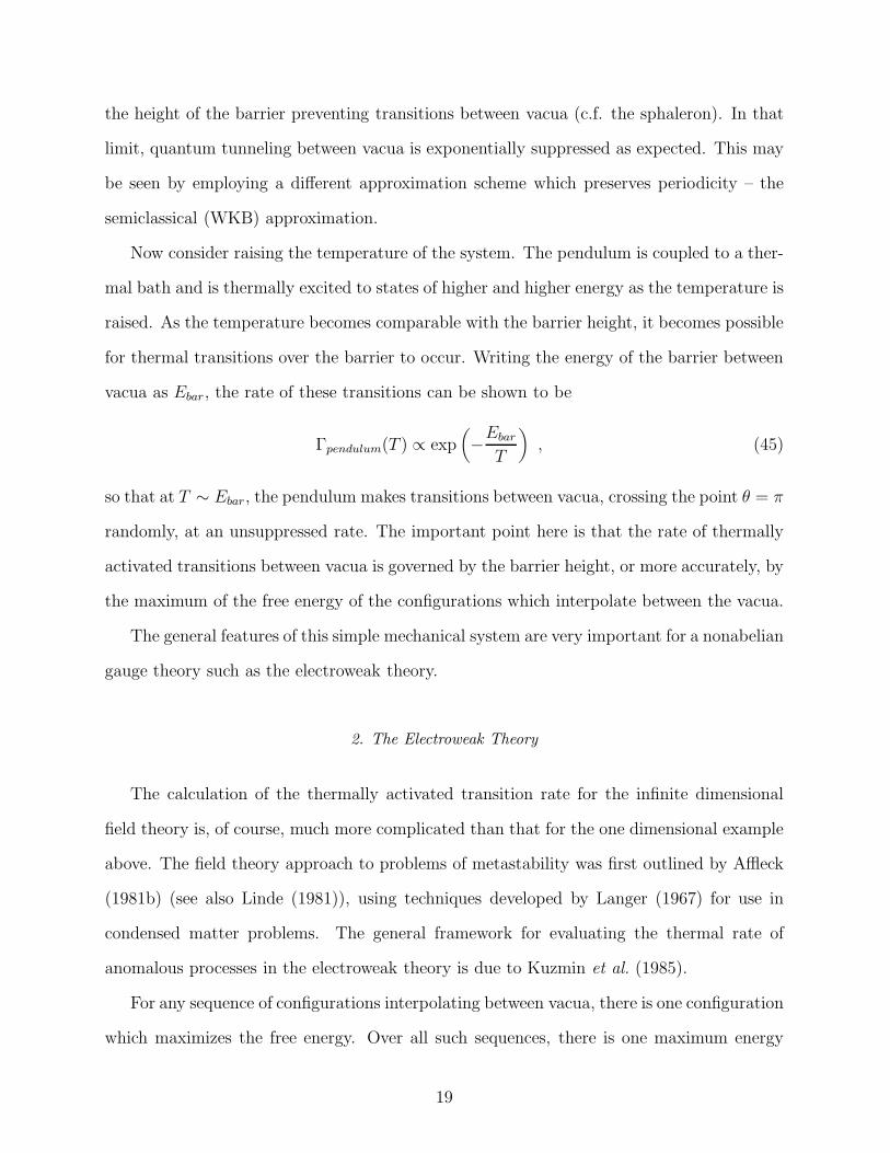
Now consider raising the temperature of the system. The pendulum is coupled to a ther-
mal bath and is thermally excited to states of higher and higher energy as the temperature is
raised. As the temperature becomes comparable with the barrier height, it becomes possible
for thermal transitions over the barrier to occur. Writing the energy of the barrier between
vacua as Ebar, the rate of these transitions can be shown to be
Γpendulum(T ) ∝ exp(
−EbarT
)
, (45)
so that at T ∼ Ebar, the pendulum makes transitions between vacua, crossing the point θ = π
randomly, at an unsuppressed rate. The important point here is that the rate of thermally
activated transitions between vacua is governed by the barrier height, or more accurately, by
the maximum of the free energy of the configurations which interpolate between the vacua.
The general features of this simple mechanical system are very important for a nonabelian
gauge theory such as the electroweak theory.
2. The Electroweak Theory
The calculation of the thermally activated transition rate for the infinite dimensional
field theory is, of course, much more complicated than that for the one dimensional example
above. The field theory approach to problems of metastability was first outlined by Affleck
(1981b) (see also Linde (1981)), using techniques developed by Langer (1967) for use in
condensed matter problems. The general framework for evaluating the thermal rate of
anomalous processes in the electroweak theory is due to Kuzmin et al. (1985).
For any sequence of configurations interpolating between vacua, there is one configuration
which maximizes the free energy. Over all such sequences, there is one maximum energy
19

configuration with the smallest free energy (i.e. a saddle point) and it is this configuration,
in analogy with the pendulum example, which governs the rate of anomalous transitions due
to thermal activation.
In the electroweak theory the relevant saddle point configuration is the sphaleron. In the
full Glashow-Salam-Weinberg theory, the sphaleron solution cannot be obtained analytically.
In fact, the original calculation of Klinkhamer and Manton (1984) was performed in the
SU(2)+ Higgs theory, and identified a sphaleron with energy in the range
8TeV < Esph < 14TeV , (46)
depending on the Higgs mass. The corresponding object in the full electroweak theory can
then be obtained from the SU(2) sphaleron by a perturbative analysis in which the small
parameter is the weak mixing angle θW .
To calculate the thermal baryon number violation rate, the following steps are performed.
One first computes the rate to cross the barrier over the sphaleron beginning from a given
state. This process is essentially a one degree of freedom process since all field directions
perpendicular to the negative mode corresponding to the sphaleron are ignored. The second
step is to sum over all such paths, weighting each by the appropriate Boltzmann factor. The
calculation for the electroweak theory, properly taking into account the translational and
rotational zero modes of the sphaleron, was first carried out by Arnold and McLerran (1987).
A final step is to take account of the infinity of directions transverse to the sphaleron by
performing a calculation of the small fluctuation determinant around the sphaleron. This
final step is carried out within the Gaussian approximation, and was originally performed
by Carson and McLerran (1990) (see also Carson et al. (1990)), with more recent analyses
by Baacke and Junker (1993), Baacke and Junker (1994a) and Baacke and Junker (1994b).
If MW (T ) is the thermal W boson mass calculated from the finite temperature effective
potential (see next section), the approximations which go into this calculation are valid only
in the regime
MW (T ) ≪ T ≪ MW (T )
αW. (47)
20

The rate per unit volume of baryon number violating events in this range is calculated to
be
Γ(T ) = µ(
MW
αWT
)3
M4W exp
(
−Esph(T )
T
)
, (48)
where µ is a dimensionless constant. Here, the temperature-dependent “sphaleron” energy
is defined through the finite temperature effective potential by
Esph(T ) ≡ MW (T )
αWE , (49)
with the dimensionless parameter E lying in the range
3.1 < E < 5.4 , (50)
depending on the Higgs mass.
Recent approaches to calculating the rate of baryon number violating events in the
broken phase have been primarily numerical. Several results using real time techniques
(Tang and Smit, 1996; Moore and Turok, 1997a) were found to contain lattice artifacts
arising from an inappropriate definition of NCS. These techniques were later shown to be
too insensitive to the true rate when improved definitions of NCS were used (Moore and
Turok, 1997b; Ambjørn and Krasnitz, 1997). The best calculation to date of the broken
phase sphaleron rate is undoubtably that by Moore (1998a). This work yields a fully non-
perturbative evaluation of the broken phase rate by using a combination of multicanonical
weighting and real time techniques.
Although the Boltzmann suppression in (48) appears large, it is to be expected that, when
the electroweak symmetry becomes restored (Kirzhnits, 1972; Kirzhnits and Linde, 1972)
at a temperature of around 100 GeV, there will no longer be an exponential suppression
factor. Although calculation of the baryon number violating rate in the high temperature
phase is extremely difficult, a simple estimate is possible. In Yang-Mills Higgs theory at
nonzero temperature the infrared modes (those with wavenumber k ≪ T ) are well described
classically in the weak coupling limit, while the ultraviolet modes (k ∼ T ) are not. Now,
the only important scale in the symmetric phase is the magnetic screening length given by
21

ξ = (αWT )−1 . (51)
Assuming that any time scale must also behave in this way, then on dimensional grounds,
we expect the rate per unit volume of baryon number violating events, an infrared spacetime
rate, to be
Γ(T ) = κ(αWT )4 , (52)
with κ another dimensionless constant, assuming that the infrared and ultraviolet modes
decouple from each other.
The rate of baryon number violating processes can be related to the sphaleron rate,
which is the diffusion constant for Chern-Simons number (20) and is defined by
limV→∞
limt→∞
[
〈(NCS(t) −NCS(0))2〉V t
]
, (53)
(c.f. (30)) by a fluctuation-dissipation theorem (Khlebnikov and Shaposhnikov, 1988) (for a
good description of this see Rubakov and Shaposhnikov (1996)). In almost all numerical cal-
culations of the baryon number violation rate, this relationship is used and what is actually
evaluated is the diffusion constant. The first attempts to numerically estimate κ in this way
(Ambjørn et al., 1990; Ambjørn et al., 1991) yielded κ ∼ 0.1− 1, but the approach suffered
from limited statistics and large volume systematic errors. Nevertheless, more recent nu-
merical attempts (Ambjørn and Krasnitz, 1995; Moore, 1996; Tang and Smit, 1996; Moore
and Turok, 1997a) found approximately the same result. However, as I mentioned above,
these approaches employ a poor definition of the Chern-Simons number which compromises
their reliability.
The simple scaling argument leading to (52) has been recently criticized by Arnold et al.
(1997) who argue that damping effects in the plasma suppress the rate by an extra power of
αW . The essential reason for the modification is that the decoupling between infrared and
ultraviolet modes does not hold completely when dynamics are taken into account. Since the
transition rate involves physics at soft energies g2T that are small compared to the typical
hard energies ∼ T of the thermal excitations in the plasma, the simplest way of analyzing
22

the problem is to consider an effective theory for the soft modes. Thus, one integrates out
the hard modes and keeps the dominant contributions, the so-called hard thermal loops. It
is the resulting typical frequency ωc of a gauge field configuration with spatial extent (g2T )−1
immersed in the plasma that determines the change of baryon number per unit time and
unit volume. This frequency has been estimated to be
ωc ∼ g4T , (54)
when the damping effects of the hard modes (Arnold et al., 1997; Arnold, 1997) are taken
into account.
In recent months the dust has settled around these issues. The analysis of Moore and
Turok (1997b) demonstrated that, when a reliable definition of NCS is used, there is a lattice
spacing dependence in the symmetric phase rate that is consistent with the claims of Arnold
et al. (1997) and similar results were also obtained by Ambjørn and Krasnitz (1997). Huet
and Son (1997) have constructed the nonlocal infra-red effective theory which includes the
effects of hard thermal loops that they expect to be responsible for the extra power of αW
in the rate of baryon number violation. Further, a rigorous field-theoretic derivation of this
theory has been derived (Son, 1997). Using ideas developed by Hu and Mueller (1997), the
effects of hard thermal loops have also been considered in work by Moore et al. (1998) (see
also Iancu (1997)). In that work the authors find
Γ(T ≫ Tc) = κ′αW (αWT )4 , (55)
with
κ′ = 29 ± 6 (56)
for the minimal standard model value of the Debye mass. Note that, although this esti-
mate takes into account physics that did not enter the original estimate, this expression is
numerically close to (52).
Finally, the effective dynamics of soft nonabelian gauge fields at finite temperature has
been recently addressed by Bodeker (1998), who finds a further logarithmic correction
23

Γsp ∼ α5WT
4 ln(1/αW ) . (57)
The physics leading to these corrections has been discussed at length by Moore (Moore,
1998b), who describes in detail both the intuitive arguments for such a term and the lat-
tice Langevin calculations required to provide an accurate numerical determination of its
magnitude.
Now that I have discussed baryon number violation, I shall turn to the second Sakharov
criterion and its realizations in the standard model.
III. C AND CP VIOLATION
As I mentioned earlier, it is necessary that both the C and CP symmetries be violated
for baryogenesis scenarios to succeed. One cause of the initial excitement over electroweak
baryogenesis was the observation that the Glashow-Salam-Weinberg model naturally satisfies
these requirements.
Recall that fermions in the theory are chirally coupled to the gauge fields as in equa-
tion (21). This means that, for example, only the left-handed electron is SU(2) gauge
coupled. In terms of the discrete symmetries of the theory, these chiral couplings result in
the electroweak theory being maximally C-violating. This is a general feature that remains
true in extensions of the theory and makes the model ideal for baryogenesis. However, the
issue of CP-violation is more complex.
A. Standard Model CP Violation: the KM Matrix
CP is known not to be an exact symmetry of the weak interactions. This is seen ex-
perimentally in the neutral Kaon system through K0, K0 mixing (Christenson et al., 1964).
At present there is no accepted theoretical explanation of this. However, it is true that CP
violation is a natural feature of the standard electroweak model. When the expression (21)
24

is expanded to include N generations of quarks and leptons, there exists a charged current
which, in the weak interaction basis, may be written as
LW =g√2ULγ
µDLWµ + (h.c.) , (58)
where UL = (u, c, t, . . .)L and DL = (d, s, b, . . .)L. Now, the quark mass matrices may be
diagonalized by unitary matrices V UL , V U
R , V DL , V D
R via
diag(mu, mc, mt, . . .) = V UL M
UV UR , (59)
diag(md, ms, mb, . . .) = V DL M
DV DR . (60)
Thus, in the basis of quark mass eigenstates, (58) may be rewritten as
LW =g√2U ′LKγ
µD′LWµ + (h.c.) , (61)
where U ′L ≡ V U
L UL and D′L ≡ V D
L DL. The matrix K, defined by
K ≡ V UL (V D
L )† , (62)
is referred to as the Kobayashi-Maskawa (KM) quark mass mixing matrix (Kobayashi and
Maskawa, 1973). For N generations, K contains (N − 1)(N − 2)/2 independent phases, and
a nonzero value for any of these phases signals CP violation. Therefore, CP violation exists
for N ≥ 3 and when N = 3, as in the standard model, there is precisely one such phase
δ. While this is encouraging for baryogenesis, it turns out that this particular source of CP
violation is not strong enough. The relevant effects are parameterized by a dimensionless
constant which is no larger than 10−20. This appears to be much too small to account for the
observed BAU and, thus far, attempts to utilize this source of CP violation for electroweak
baryogenesis have been unsuccessful.
When one includes the strong interactions described by quantum chromodynamics
(QCD), a second potential source of CP violation arises due to instanton effects. How-
ever, precision measurements of the dipole moment of the neutron constrain the associated
dimensionless parameter θQCD to be less than 10−9, which again is too small for baryogene-
sis. In light of these facts, it is usual to extend the standard model in some minimal fashion
25

that increases the amount of CP violation in the theory while not leading to results that
conflict with current experimental data.
B. The Two-Higgs Doublet Model
One particular way of achieving this (McLerran, 1989) is to expand the Higgs sector of
the theory to include a second Higgs doublet. In a two-Higgs model, the structure described
in section II is doubled so that we have scalars Φ1 and Φ2, and the scalar potential is replaced
by the most general renormalizable two-Higgs potential (Gunion et al., 1989)
V (Φ1,Φ2) = λ1(Φ†1Φ1 − v2
1)2 + λ2(Φ
†2Φ2 − v2
2)2
+ λ3[(Φ†1Φ1 − v2
1) + (Φ†2Φ2 − v2
2)]2
+ λ4[(Φ†1Φ1)(Φ
†2Φ2) − (Φ†
1Φ2)(Φ†2Φ1)]
+ λ5[Re(Φ†1Φ2) − v1v2 cos ξ]2
+ λ6[Im(Φ†1Φ2) − v1v2 sin ξ]2 . (63)
Here v1 and v2 are the respective vacuum expectation values of the two doublets, the λi are
coupling constants, and ξ is a phase. To make the CP-violation explicit, let us write the
Higgs fields in unitary gauge as
Φ1 = (0, ϕ1)T , Φ2 = (0, ϕ2e
iθ)T , (64)
where ϕ1, ϕ2, θ are real, and θ is the CP-odd phase. The important terms for CP violation
in the potential are the final two, with coefficients λ5 and λ6, since it is these terms which
determine the dynamics of the CP-odd field θ.
There are several mechanisms by which θ may contribute to the free energy density
of the theory. To be specific, let us concentrate on the one-loop contribution (Turok and
Zadrozny, 1990) and for simplicity assume that θ is spatially homogeneous. The relevant
term is
FB = − 14
3π2nfζ(3)
(
m
T
)2
θnB , (65)
26

where m is the finite temperature mass of the particle species dominating the contribution
to the anomaly and ζ is the Riemann function.
The coefficient of nB in the above equation can be viewed as a sort of chemical potential,
µB, for baryon number
µB =14
3π2nfζ(3)
(
m
T
)2
θ . (66)
The changes in θ are dependent on changes in the magnitude of the Higgs fields. In
particular, if a point in space makes a transition from false electroweak vacuum to true
then ∆θ > 0, and sphaleron processes result in the preferential production of baryons over
antibaryons. For the opposite situation ∆θ < 0, and sphaleron processes generate an excess
of antibaryons. The total change in the phase θ (from before the phase transition to T = 0)
may be estimated to be
∆θ ∼ ξ − arctan
(
λ6
λ5
tan ξ
)
, (67)
and, as we will see, it is this quantity that enters into estimates of the BAU. This then is
how the dynamics of the two-Higgs model bias the production of baryons through sphaleron
processes in electroweak baryogenesis models. The use of the two-Higgs model is motivated
in part by supersymmetry (SUSY), which demands at least two Higgs scalars. However,
in the minimal supersymmetric standard model (MSSM), supersymmetry demands that
λ5 ≡ λ6 = 0 and so the two-Higgs potential is CP invariant. In such models CP violation
arises through soft-SUSY breaking which generates nonzero values for λ5 and λ6, as we shall
see later.
C. CP Violation from Higher Dimension Operators
The second popular method of extending the standard model is to view the model as an
effective field theory, valid at energies below some mass scale M . In addition to the standard
terms in the Lagrangian, one then expects extra, nonrenormalizable operators, some of
27

which will be CP odd (Shaposhnikov, 1988; Dine et al., 1991; Dine et al., 1992b; Zhang et
al., 1994; Lue et al., 1997). A particular dimension six example is
O =b
M2Tr(Φ†Φ)Tr(FµνF
µν) , (68)
with b a dimensionless constant. O is the lowest dimension CP odd operator which can be
constructed from minimal standard model Higgs and gauge fields. Such a term, with M = v,
can be induced in the effective action by CP violation in the CKM matrix, but in that case
the coefficient b is thought to be tiny.
The operator O induces electric dipole moments for the electron and the neutron (Zhang
and Young, 1994), and the strongest experimental constraint on the size of such an operator
comes from the fact that such dipole moments have not been observed. Working to lowest
order (one-loop) Lue et al. (1997) find
dee
=me sin2(θW )
8π2
b
M2ln
(
M2 +m2H
m2H
)
. (69)
Note that M2 arises in the logarithm without b because M , the scale above which the
effective theory is not valid, is the ultraviolet cutoff for the divergent loop integral. Using
the experimental limit (Commins et al., 1994)
dee< 4 · 10−27cm (70)
yields the bound
b
M2ln
(
M2 +m2H
m2H
)
<1
(3 TeV)2. (71)
The corresponding experimental limit (Smith et al, 1990; Altarev et al., 1992) on the neutron
electric dipole moment dn is weaker than that on de, but because dn is proportional to the
quark mass rather than to the electron mass, the constraint obtained using dn is comparable
to (71). Any baryogenesis scenario which relies on CP violation introduced via the operator
O must respect the bound (71).
28

D. General Treatment
Common to both the above extensions of the standard model is the appearance of extra,
CP violating interactions, parameterized by a new quantity δCP (e.g. δ = ∆θ or δ = b/M2).
Although there exist a number of other ways in which CP violation may appear in low
energy electroweak models (see, for example (Frere et al., 1993; Reina and Tytgat, 1994)),
in many parts of this review, for definiteness, I shall focus on ∆θ. However, in the discussion
of specific SUSY models I shall explain how CP violating quantities arise. Whatever its
origin, the effect of CP violation on anomalous baryon number violating processes is to
provide a fixed direction for the net change in baryon number. When the bias is small, the
equation governing this can be derived from detailed balance arguments (Khlebnikov and
Shaposhnikov, 1988; Dine et al., 1990) and may be written as
dnBdt
= −3Γ(T )
T∆F , (72)
where ∆F is the free energy difference, induced by the CP violation, between producing
baryons and antibaryons in a given process, and Γ is the rate per unit volume of baryon
number violating events. I shall use this equation further when considering nonlocal baryo-
genesis.
IV. THE ELECTROWEAK PHASE TRANSITION
To begin with I shall lay down some definitions from thermodynamics. If a thermody-
namic quantity changes discontinuously (for example as a function of temperature) then we
say that a first order phase transition has occurred. This happens because, at the point
at which the transition occurs, there exist two separate thermodynamic states that are in
equilibrium. Any thermodynamic quantity that undergoes such a discontinuous change at
the phase transition is referred to as an order parameter, denoted by ϕ. Whether or not a
first order phase transition occurs often depends on other parameters that enter the theory.
It is possible that, as another parameter is varied, the change in the order parameter at the
29

phase transition decreases until it, and all other thermodynamic quantities are continuous at
the transition point. In this case we refer to a second order phase transition at the point at
which the transition becomes continuous, and a continuous crossover at the other points for
which all physical quantities undergo no changes. In general, we are interested in systems
for which the high temperature ground state of the theory is achieved for ϕ = 0 and the low
temperature ground state is achieved for ϕ 6= 0.
The question of the order of the electroweak phase transition is central to electroweak
baryogenesis. Phase transitions are the most important phenomena in particle cosmology,
since without them, the history of the universe is simply one of gradual cooling. In the
absence of phase transitions, the only departure from thermal equilibrium is provided by
the expansion of the universe. At temperatures around the electroweak scale, the expansion
rate of the universe in thermal units is small compared to the rate of baryon number violating
processes. This means that the equilibrium description of particle phenomena is extremely
accurate at electroweak temperatures. Thus, baryogenesis cannot occur at such low scales
without the aid of phase transitions (for a treatment of this argument in the context of non-
standard cosmologies, in which the universe is not radiation dominated at the electroweak
scale, see Joyce and Prokopec (1998)).
For a continuous transition, the extremum at ϕ = 0 becomes a local maximum at Tc and
thereafter there is only a single minimum at ϕ 6= 0 (see figure 5). At each point in space
thermal fluctuations perturb the field which then rolls classically to the new global minimum
of the FTEP. Such a process is referred to as spinodal decomposition. If the EWPT is second
order or a continuous crossover, the associated departure from equilibrium is insufficient to
lead to relevant baryon number production (Kuzmin et al., 1985). This means that for
EWBG to succeed, we either need the EWPT to be strongly first order or other methods
of destroying thermal equilibrium, for example topological defects (see section VIII), to be
present at the phase transition.
For a first order transition the extremum at ϕ = 0 becomes separated from a second
local minimum by an energy barrier (see figure 4). At the critical temperature T = Tc
30

both phases are equally favored energetically and at later times the minimum at ϕ 6= 0
becomes the global minimum of the theory. The dynamics of the phase transition in this
situation is crucial to most scenarios of electroweak baryogenesis. The essential picture is
that at temperatures around Tc quantum tunneling occurs and nucleation of bubbles of
the true vacuum in the sea of false begins. Initially these bubbles are not large enough
for their volume energy to overcome the competing surface tension and they shrink and
disappear. However, at a particular temperature below Tc bubbles just large enough to
grow nucleate. These are termed critical bubbles, and they expand, eventually filling all of
space and completing the transition. As the bubble walls pass each point in space, the order
parameter changes rapidly, as do the other fields, and this leads to a significant departure
from thermal equilibrium. Thus, if the phase transition is strongly enough first order it is
possible to satisfy the third Sakharov criterion in this way.
There exists a simple equilibrium analysis of bubble nucleation in a first order phase
transition (see, for example, Rubakov and Shaposhnikov (1996)). Write the bubble nucle-
ation rate per unit volume at temperature T as R(T ). Further, note that if we assume that
bubbles expand at constant speed v, then the volume occupied at time t by a bubble that
nucleated at time t0 is
V (t, t0) =4π
3(t− t0)
3v3 . (73)
Then, the fraction of the total volume occupied by the broken phase at time t can be written
as
P (t) = 1 − exp[−Σ(t)] , (74)
where the quantity Σ(t) is given by
Σ(t) =∫ t
tcdt0 V (t, t0)R(T0) (75)
and tc and T0 are defined through T (tc) = Tc and T (t0) = T0 respectively. In terms of this
quantity, we say that the phase transition is complete when Σ ≃ 1. In order to estimate
Σ(t) note that when bubble nucleation begins, the quantity
31

x ≡ Tc − T
Tc(76)
is small. Making this change of variables in (75), and using the time-temperature relationship
t = M/T 2, with M ∼ 1018GeV we obtain, for small x
Σ(t) =64πv3
3
(
M
Tc
)4∫ x
0dx x3 1
T 4c
R(T ) . (77)
Note that, from this expression, it is clear that when Σ is of order one, when the phase
transition completes or percolates, the rate per unit volume is negligibly small.
In general, the calculation of the bubble nucleation rate is extremely complicated. The
relevant time scale τform for the formation of a critical bubble is of the form
τform ∝ exp(Fc/T ) , (78)
where Fc is the free energy of the bubble configuration. We may calculate this by writing the
bubble as a spherically symmetric configuration ϕ(r) which extremizes the effective action
(as defined in the next subsection) and satisfies
limr→∞
ϕ(r)= 0 ,
ϕ(0)= v(T )
where v(T ) is the minimum of the finite temperature effective potential V (ϕ, T ) defined
properly in the next subsection. Then the free energy is given by
Fc[ϕ(r)] ≃∫
dr r2[
1
2(ϕ′)2 + V (ϕ, T )
]
(79)
with the bubble configuration obtained by solving
1
r2
d
dr(r2ϕ′) − ∂V
∂ϕ= 0 (80)
subject to the above boundary conditions. However, in the general situation these equations
must be solved numerically, although some progress can be made in the thin wall limit in
which the typical size of the critical bubbles is much larger than the correlation length of
the system.
32

The precise evolution of critical bubbles in the electroweak phase transition is a crucial
factor in determining which regimes of electroweak baryogenesis are both possible and effi-
cient enough to produce the BAU. In essence, the bubble wall dynamics is governed by the
interplay between the surface tension and the volume pressure.
The physics of a propagating phase boundary, or bubble wall, have been extensively
investigated by many authors (Enqvist et al., 1992; Dine et al., 1992a; Turok, 1992; Liu et
al., 1992; Khlebnikov, 1992; Arnold, 1993; Huet and et al., 1993; Laine, 1994; Ignatius et
al., 1994; Kurki-Suonio and Laine, 1995; Heckler, 1995; Funakubo et al., 1995; Moore and
Prokopec, 1995a; Moore and Prokopec, 1995b; Kurki-Suonio and Laine, 1996a; Kurki-Suonio
and Laine, 1996b; Duari and Yajnik, 1996; Funakubo et al., 1997). The crucial quantities
that one wishes to estimate are the wall velocity, v, and the wall width, δ. As will become
clear later, it is important to know whether the velocity is less than or greater than the
speed of sound in the plasma, because different mechanisms of baryogenesis dominate in
these regimes. As it turns out, the dynamics of the bubble wall is qualitatively different in
these two regimes also (Steinhardt, 1982; Gyulassy et al., 1983).
To be definite, consider a single bubble of broken electroweak symmetry expanding in a
sea of symmetric phase plasma, and for simplicity assume that the bubble is large enough
that we may neglect its curvature and idealize the wall as a planar interface. There are two
relevant regimes:
1. The wall velocity is less than the speed of sound (v < cs ≃ 0.58): In this case it is
said that deflagration occurs. The plasma near the bubble wall in the unbroken phase
accelerates away from the wall and a shock wave develops ahead of the wall moving at
speed vsw > v. This results in the heating of the plasma behind the shock front (For
a detailed treatment of deflagration see Kurki-Suonio (1985)).
2. The wall velocity is greater than the speed of sound (v > cs): In this case we refer to
detonation occurring. In contrast to deflagration, the plasma ahead of the wall is now
at rest, whereas that behind the wall in the broken phase accelerates away.
33

Which of these regimes is relevant for a given phase transition depends on a host of
microphysical inputs, making an analytic approach extremely difficult. However, recent
investigations of the bubble wall behavior in the standard model have been performed (Moore
and Prokopec, 1995a; Moore and Prokopec, 1995b). These authors find that if mH < 90 GeV
(encompassing the whole region of physically allowed Higgs masses for which a strongly
first order phase transition is expected to occur), the phase transition proceeds through
deflagration. They find a robust upper bound on bubble velocities
v < 0.45 < vsw ≃ cs ≃ 0.58, mH < 90GeV (81)
Other recent work (Moore and Turok, 1997b) has demonstrated the importance of friction
from infrared W bosons on the wall velocity and suggests that velocities of the order
v ∼ 0.1 − 0.2 (82)
may be realistic. Of course, the methods used in this analysis cannot be extended past the
point at which the shock waves originating from different bubbles would collide, since at
that stage the approximation of an isolated wall is no longer valid. In fact, the dynamics of
the phase transition from that point to completion is quite different from the simple picture
I have described above. What seems clear is that significant heating of the plasma occurs,
perhaps up to Tc (Kurki-Suonio and Laine, 1996b), as the latent heat of the transition is
released. This should result in an appreciable deceleration of the bubble walls until finally,
the transition is completed by relatively slow moving bubbles. In fact, some analytical
progress may be made in the limit in which one assumes that the latent heat of the transition
is released instantaneously into the plasma (Heckler, 1995). While all these approaches are
useful in understanding the nature of bubble walls, it is important to remember that they are
performed in the minimal standard model. When a particular extension of the electroweak
theory is used, the analysis should be repeated in that context.
In practice it can be a difficult task to determine the order of a given phase transition
and thus whether, and how, bubble walls may arise. In the remainder of this section I shall
34

review some of the analytical and numerical approaches which are used, and discuss their
application to the electroweak phase transition.
A. The finite temperature effective potential
A widely used tool in studying thermal phase transitions is the finite temperature effective
potential (FTEP) for the order parameter. I have already mentioned this in passing when
discussing bubble nucleation. Here I will define this object precisely, and explain how it is
calculated in a simple model. I will then give the form of the potential for the electroweak
theory and show how it is used.
Let us begin at zero temperature and consider a single scalar field ϕ with external source
J . The generating functional for this theory is
Z[J ] =∫
Dϕ exp[
i∫
d4x (L[ϕ] + Jϕ)]
. (83)
From this quantity the field theory analog E[J ] of the Helmholtz free energy is defined by
e−iE[J ] ≡ Z[J ] . (84)
As is well known, functional differentiation of E[J ] with respect to the source J defines the
classical field through
δ
δJ(x)E[J ] = −ϕcl . (85)
Now, in thermodynamics it is usual to construct the Gibbs free energy of the theory by a
Legendre transform of the Helmholtz free energy. In field theory we perform an analogous
transformation to define the effective action by
Γ[ϕcl] ≡ −E[J ] −∫
d4y J(y)ϕcl(y) . (86)
This functional has the useful property that
J(x) = − δ
δϕcl(x)Γ[ϕcl] , (87)
35

which means that, in the absence of an external source, the effective action defined by (86)
satisfies
δ
δϕcl(x)Γ[ϕcl] = 0 . (88)
Thus, the values of the classical fields in the vacua of the theory are obtained by solving this
equation, i.e., by extremizing the effective action.
One further simplification is possible. If the vacua of the theory are translation and
Lorentz invariant, then ϕcl is constant. In that case, Γ[ϕcl] contains no derivatives of ϕcl
and (88) is an ordinary equation. It is therefore convenient to define the effective potential
by
Veff(ϕcl) ≡ − 1
V4
Γ[ϕcl] , (89)
where V4 is the spacetime 4-volume, so that the equation leading to the vacua of the theory
reduces to
∂
∂ϕclVeff(ϕcl) = 0 . (90)
Note that this equation allows one, in principle, to compute the vacua of the theory exactly,
taking into account all corrections to the bare potential from quantum fluctuations in the
field ϕ.
Exact analytic calculations of the effective potential are difficult. Therefore, it is usual
to use perturbation theory. As an example, in the scalar field model above choose the bare
potential to be
V (ϕ) = −µ2
2ϕ2 +
λ
4ϕ4 , (91)
with µ an arbitrary mass scale and λ a parameter. We write ϕ as
ϕ(x) = ϕcl + χ(x) , (92)
and the aim is to take account of the small quantum fluctuations in χ around the classical
vacuum state ϕcl. These fluctuations can contribute to both the energy of the vacuum state
36

and the potential felt by ϕcl, since the mass of the field χ is due to ϕcl. The perturbation
theory approach to calculating the effects of quantum fluctuations is usually phrased in the
language of Feynman diagrams. At the one-loop level, there is only one diagram, which is a
single χ loop. This loop yields a contribution to the effective potential of
V (1)(ϕcl) =1
2(2π)4
∫
d4k ln[k2 + 3λϕ2cl − µ2] . (93)
If we perform the k0 integration and remove an infinite constant, this becomes
V (1)(ϕcl) =1
(2π)3
∫
d3k k[|k|2 + 3λϕ2cl − µ2]1/2 . (94)
This expression can now be seen to correspond to an integral over the energy of a χ particle
in all momentum modes. Note that, since this energy depends on ϕcl, normal ordering
cannot remove this contribution to the energy.
Since (94) is divergent, we must choose renormalization conditions to perform the integra-
tion. If we choose to renormalize at the point ϕ = µλ−1/2, and there set V ′(ϕ) = V ′′(ϕ) = 0,
then the one loop zero temperature effective potential becomes
V(1)eff(ϕ) = −µ
2
2ϕ2 +
λ
4ϕ4 +
1
64π2(3λϕ2 − µ2)2 ln
(
3λϕ2 − µ2
2µ2
)
+21λµ2
64π2ϕ2 − 27λ2
128π2ϕ4 . (95)
We now wish to incorporate the effects of thermal fluctuations into this picture. Just as
quantum fluctuations of fields lead to a modification of the potential, thermal fluctuations
have an analogous effect. The potential resulting from taking account of thermal fluctua-
tions is referred to as the finite temperature effective potential (FTEP). The formalism we
set up for the zero temperature case is applicable here also because of the well-known con-
nection between zero-temperature field theory and thermal field theory. The path integral
formulation of field theory at nonzero temperature T, describing the equilibrium structure
of the theory, is formally equivalent to the zero temperature formalism performed over a Eu-
clidean time interval of length β ≡ 1/T . In addition, one must impose appropriate boundary
37

conditions on the fields; periodic for bosons and anti-periodic for fermions. Thus, any field
χ may be Fourier expanded over this Euclidean time interval, yielding the expression
χ(x, τ) =∞∑
n=−∞
χn(x)eiωnτ , (96)
with
ωn =
2nπT Bosons
(2n+ 1)πT Fermions. (97)
Since the Euclidean time coordinate is now finite, the zeroth component of a particle’s
four momentum is now discrete. When we perform an integral over k0, as in the quantum
case above, this becomes a sum. This means that the one loop temperature dependent
contribution to the FTEP is
V (1)(ϕ, T ) =T
2(2π)3
+∞∑
n=−∞
∫
d3k ln[(2πnT )2 + |k|2 + 3λϕ2 − µ2] . (98)
If we define m2(ϕ) ≡ 3λϕ2 − µ2, then for m ≪ T we may perform the sum and integral to
first order in lambda. After renormalization we add this to the bare potential to give the
one loop FTEP as
V(1)eff (ϕ, T ) = −µ
2
2ϕ2 +
λ
4ϕ4 +
m2(ϕ)
24T 2 − π2
90T 4 . (99)
This can be thought of as the contribution to the ϕ-potential from the energy of, and
interaction with, a thermal bath of particles at temperature T .
In general, in a theory with spontaneous symmetry breaking, the usual high temperature
behavior of the theory is that of the zero temperature theory at high energies. That is to
say that the full symmetry of the Lagrangian is restored at high temperatures. At high
temperatures the global minimum of the FTEP is at ϕ = 0 and at zero temperature the
global minimum is at ϕ = v, where v is the usual Higgs vacuum expectation value (VEV).
In the standard electroweak theory (ignoring the U(1) terms) the high temperature form
of the one loop FTEP is
38

V(1)eff(ϕ;T ) =
(
3
32g2 +
λ
4+m2t
4v2
)
(T 2 − T 2∗ )ϕ2 − 3g2
32πTϕ3 +
λ
4ϕ4 , (100)
with ϕ ≡√
φ†φ, and mt the top quark mass. Note that, in calculating this quantity for a
gauge theory, one also takes into account loop diagrams corresponding to fluctuations in the
gauge fields. The lowest order thermal correction to the zero temperature effective potential
is a temperature dependent mass. It is this contribution that causes the extremum at ϕ = 0
to be the global minimum at high temperatures. Note also the presence of a cubic term in
the effective potential. This term arises from the gauge field fluctuations, and is responsible
for the existence of a barrier separating two degenerate vacua at the critical temperature,
and hence for the prediction that the electroweak phase transition be first order. Using
this one loop potential, we may estimate the critical temperature at which the vacua are
degenerate to be
Tc = mH
(
3
8g2 + λ− 9
256π2g6 +
m2t
v2
)−1/2
. (101)
Calculations of quantities such as the critical temperature can be refined if the effective
potential is calculated to higher orders in perturbation theory. In particular, nowadays the
two-loop calculation has been performed (Arnold and Espinosa, 1993; Fodor and Hebecker,
1994; Farakos et al., 1994a; Farakos et al., 1994b; Buchmuller et al., 1995).
It is worthwhile including a cautionary note concerning the FTEP. If the interactions are
weak, i.e. if
g2T
πmW (ϕ)≪ 1 , (102)
then the effective potential approach is equivalent to solving the full equations of motion
for the gauge and Higgs fields with all fluctuations taken into account. However, in a
perturbative approximation it is very difficult to go beyond two loops, which limits the
accuracy of the method. Further, when the phase transition is weak, the infrared degrees of
freedom become strongly coupled (Linde, 1980; Gross et al., 1981), the inequality (102) is
no longer satisfied, and we must turn to numerical approaches.
39

Note that the higher the Higgs mass is, the weaker the phase transition gets. The current
lower bound on the mass of the Higgs in the minimal standard model (MSM) comes from
combining the results of the DELPHI, L3 and OPAL experiments at LEP and is
mH > 89.3 GeV (103)
(de Jong, 1998) and so the perturbation expansion might not be expected to converge.
B. Dimensional Reduction
As I have already explained, equilibrium field theory at nonzero temperature can be
formulated as zero temperature field theory performed over a finite interval of Euclidean
time with period 1/T .
If we expand the fields as in (97), one may think of the theory as a three dimensional
system of an infinite number of fields χn. These fields comprise a tower of states of increasing
masses proportional to the Matsubara frequencies ωn. If the theory is weakly coupled (as we
expect), then we may make a simplifying approximation. For momenta much less that the
temperature, we may perturbatively account for the effects of all fields with nonzero thermal
masses. Thus, since all the fermions are massive, what remains is an effective theory of only
the bosonic fields with n = 0, the zero modes.
To see how the remaining fields contribute to the dynamics of such a theory consider the
following equivalent construction. Write down the most general, renormalizable Lagrangian
for the zero modes in three dimensions. For this to be the effective theory we seek, it is
necessary that the free parameters be determined by matching the one-particle irreducible
(1PI) Green’s functions with those of the full theory in four dimensions. The massive degrees
of freedom are important for this matching condition and thus contribute to the masses and
couplings in the three-dimensional effective theory.
The three-dimensional effective theory is much simpler than the full theory. For the
MSM, the particle content is the Higgs doublet, the 3d SU(2) × U(1) gauge fields, and
40

extra bosonic fields corresponding to the temporal components of the gauge fields in the full
theory. For this effective theory, perturbative calculations of the coupling constants to one
loop (Farakos et al., 1994a) and masses to second order (Kajantie et al., 1996a) have been
performed.
In the region of the phase transition itself, a further simplification is possible. In this
regime, the masses of the extra bosons in the theory are proportional to gT or to g′T and are
heavy compared to the effective Higgs mass of the theory. Thus, we may integrate out these
heavy degrees of freedom and obtain a simple, effective 3d theory which describes the system
near the phase transition (Ginsparg, 1980; Applequist and Pisarski, 1981; Nadkarni, 1983;
Landsman, 1989; Farakos et al., 1994a; Farakos et al., 1994b; Laine, 1995). The appropriate
Lagrangian is
L =1
4W aijW
aij +
1
4FijFij + (Diφ)†Diφ+m2
3φ†φ+ λ3(φ
†φ)2 , (104)
where m3 and λ3 are the effective 3d Higgs mass and self-coupling in the theory near the
phase transition.
This theory is superrenormalizable since m23 has only linear and log divergences and, in
the MS scheme, λ3 and g3, the 3-dimensional gauge coupling, do not run at all. Thus,
the theory described by (104) is very powerful, since the perturbative calculations of the
parameters involved do not suffer from any infrared divergences. As a result, the theory is
valid over a large range
30GeV < mH < 240GeV (105)
of Higgs masses. In addition, removal of the ultraviolet divergences of the theory is simple.
Further, the vastly decreased number of degrees of freedom makes the analysis of this theory
much more manageable. One might wonder if the results from this approach can be checked
against those from the full 4d theory in any regimes. In fact, at high temperatures, calcu-
lations of the 4d effective potential in which hard thermal loops are “resummed” (Arnold
and Espinosa, 1993; Fodor and Hebecker, 1994; Farakos et al., 1994a) agree well with the 3d
41

results (for a nonperturbative approach to checking this agreement see Laine (1996b). For
an alternative treatment of the effective 3d theory, in which a cutoff is introduced rather
than explicitly using the superrenormalizability of the theory, see (Karsch et al., 1996)
While we may construct the 3d effective theory without worrying about divergences in its
parameters, perturbative calculations using the theory are infrared divergent in the symmet-
ric phase of the system. This means that perturbation theory is not a particularly effective
tool and nonperturbative approaches are necessary. It is usual to treat the simpler SU(2)
system, in which the U(1)Y interactions are ignored, to gain insight into the nonperturbative
dynamics of the electroweak phase transition. In the context of the 3d effective theory I
have described, a number of nonperturbative methods have been used by different groups.
C. Numerical Simulations – Lattice Approaches
The second approach which has been very successful for analyzing the nature of phase
transitions at nonzero temperatures is to simulate the systems numerically on a lattice.
These approaches are technically difficult to perform but have the advantage of covering
the entire range of parameter space which might be interesting for EWBG. Here I shall
provide an outline of how these approaches are performed and give the essential results.
Numerical simulations of the electroweak phase transition have been performed in both the
3d theory described above and in the full 4d theory (Csikor et al., 1996). However, in the
4d simulations the situation is complicated in the physically allowed range of Higgs masses.
Nevertheless, considerable progress has been made.
Reliable quantitative results for the order of the EWPT have been obtained from lattice
Monte Carlo simulations of the effective 3d theory (Kajantie et al., 1993; Farakos et al.,
1994b; Farakos et al., 1994c; Kajantie et al., 1996a; Kajantie et al., 1996b; Kajantie et
al., 1996c; Kajantie et al., 1996d; Dosch et al., 1996; Dosch et al., 1997; Gurtler et al.,
1997a; Gurtler et al., 1997b; Gurtler et al., 1998a; Gurtler et al., 1998b). This approach is
technically complicated and one must take great care to ensure that the observed features
42

are not artifacts of the lattice implementation of the theory. For a discussion of these matters
and an excellent comprehensive treatment of the method, I refer the reader to Kajantie et
al. (1996b). The Monte Carlo calculations are performed over a range of system volumes V
and lattice spacings a. The important results are obtained in the limit of extrapolation to
infinite volume (V → ∞) and zero lattice spacing (a → 0). Here, I shall just sketch how
these lattice Monte Carlo calculations are performed.
The most widely studied lattice model is the pure SU(2) theory. The parameters of the
3d theory are matched with those of the 4d continuum theory by renormalization group
methods. In particular, the top quark mass is matched to the known value mt ≃ 175 GeV.
More recently, the full bosonic 3d SU(2) × U(1) theory has been simulated (Kajantie et
al., 1996c).
The approach of Kajantie et al. is to measure the volume (finite size) behavior of the
susceptibility χ of the operator φ†φ. The susceptibility is defined in terms of quantities in
the 3d effective Lagrangian (104) by
χ ≡ g23V 〈(φ†φ− 〈φ†φ〉)2〉 . (106)
For a given Higgs mass, the procedure is as follows. The first step is, at fixed volume V , to
determine the maximum value χmax of χ as a function of temperature. This procedure is
then performed over a range of V to give χmax(V ). From finite size scaling arguments, the
following behaviors are expected
χmax(V ) ∝
V First Order Transition
V γ/3 Second Order Transition
const. No Transition
, (107)
with γ 6= 0, 3 a critical exponent. Using this criterion, it is possible to infer the nature of
the phase transition from the numerical simulations. A summary of the results (Kajantie et
al., 1996d) is shown in figure (6). The general result of the Monte Carlo approach is that
the phase transition is first order for Higgs masses mH ≤ 80 GeV and becomes a smooth
crossover for mH ≥ 80 GeV. The existence of the endpoint of first order phase transitions
43

was shown by Kajantie et al. (1996d), and the position of the endpoint was identified by
Gurtler et al. (1997b). This endpoint, at mH ∼ 80 GeV falls into the universality class of the
3d Ising Model. The endpoint of the transition has also been examined in the 4d simulations
by Aoki (Aoki, 1997), with results in agreement with the 3d simulations.
Although the results I quote here are obtained in the SU(2) theory (equivalently
sin2 θW = 0 in SU(2) × U(1)), the effects of the additional U(1) of the true electroweak
theory have been considered by Kajantie et al. (1996c). However, while the effects of hyper-
charge strengthen the phase transition in general, the position of the endpoint is relatively
insensitive to the value od sin2 θW . I shall mention briefly in the next section how these
results compare with those obtained from other approaches.
As the Higgs mass is increased to 80 GeV from below, the strength of the first order
phase transition decreases. This behavior is quantified by the tension of the phase interface
at Tc and by the latent heat L of the transition. Both these quantities are measured in
the simulations and the expected weakening of the transition is observed. The Clausius-
Clapeyron equation
d∆p
dT=L
T, (108)
where ∆p is the difference in pressures between the symmetric and broken phases at tem-
perature T , is particularly useful here. The equation may be written as
∆〈φ†φ〉(
m2H
T 3c
)
=L
T 4c
, (109)
where ∆〈φ†φ〉 is the jump in the squared order parameter. As we shall use later, the
measurement of the latent heat from the simulations yields a value for ∆〈φ†φ〉 which we
shall find very useful when discussing local electroweak baryogenesis.
D. Other Approaches
The application of ε-expansion techniques to the electroweak phase transition was sug-
gested by Gleiser and Kolb (1993) and has been investigated in detail by Arnold and Yaffe
44
(1994). Since it is difficult to solve the 3d theory systematically using analytic methods, the
approach here is to replace the three spatial dimensions by 4 − ε dimensions. For example,
in massive φ4 theory, the 4d action is transformed to
S =∫
d4−εx[
(∂φ)2 +m2φ2 + µελφ4]
, (110)
where a mass scale µ has been introduced to keep couplings dimensionless. This class of
theories can be solved perturbatively in ε by making use of renormalization group improved
perturbation theory. The procedure is to perform the calculation of a given quantity in this
perturbative scheme to a given order in ε and then to take the 3d limit by taking ε→ 1. This
approach provides an interesting way to study phase transitions. However, its application
to the electroweak theory is complicated and the authors estimate that the results may be
accurate at the 30% level for Higgs masses below around 150 GeV, and less reliable for higher
values. Nevertheless, the prediction of ε-expansion techniques is that the phase transition
become weaker but remain first order as mH increases, even to values higher than 80 GeV.
In another approach (Buchmuller and Philipsen, 1995) the one-loop Schwinger-Dyson
equations are studied. This method predicts that the first order transitions become a smooth
cross-over for Higgs masses above 100 GeV. Although this result is in reasonable agreement
with that obtained from numerical approaches, it does rely on perturbation theory which,
as I have emphasized, should not really be trusted for mH ≥ 80 GeV.
Finally, exact renormalization group approaches have been applied to the electroweak
theory by Wetterich and coworkers (Reuter and Wetterich, 1993; Bergerhoff and Wetterich,
1995) and by Buchmuller and Fodor (1994). Again, these analyses support the results of
the numerical approaches I described earlier.
With the exception of the ε-expansion, the qualitative conclusion of the above approaches
is that there exists a critical value of the Higgs mass, below which the EWPT is first order,
and above which the transition is continuous. Since, as I have mentioned, results from LEP
(de Jong, 1998) now give mH > 89.3 GeV, it seems that the standard electroweak theory
undergoes a continuous transition at high temperatures.
45

E. Subcritical fluctuations
A central assumption of the analysis of the phase transitions that I have followed above is
that the initial state be homogeneous. If this is the case then the existence of a cubic term in
the finite temperature effective potential clearly implies that the phase transition proceeds
by the nucleation and propagation of critical bubbles of true vacuum in the homogeneous
sea of false. This result is obtained within the vacuum decay formalism which relies on
the semiclassical expansion of the effective action. This approach is valid if the system
begins homogeneously in the false vacuum state so that one may consistently sum over
small amplitude fluctuations about this state, as I described earlier. However, this picture
may not be valid if the initial state of the system is highly inhomogeneous.
The effects of these initial state inhomogeneities have been investigated using a variety
of different approaches by Gleiser and collaborators (Gleiser, 1993; Gleiser, 1994; Gleiser
and Ramos, 1994; Gleiser, 1995; Borrill and Gleiser, 1995; Gleiser and Heckler, 1996; Borrill
and Gleiser, 1997; Gleiser et al., 1997). At very high temperatures, the order parameter is
certainly well-localized about the symmetric vacuum state. However, as we approach the
critical temperature we must be sure that thermal fluctuations do not lead to significant
inhomogeneities such that the saddle point approximation breaks down. In particular, if
there is a sufficient probability for the order parameter to reach the true vacuum by purely
classical thermal processes (subcritical fluctuations) near the critical point, then we may not
apply the nucleation calculation and might expect that the transition proceeds similarly to
spinodal decomposition despite the first order nature of the effective potential.
Although quantifying this statement is highly nontrivial, recent progress has been made
numerically by Borrill and Gleiser (1995). These authors use a Langevin approach to track
the dynamics of the order parameter in a spontaneously broken theory of a real scalar field
in 3 + 1 dimensions. They use a potential which is identical in form to the electroweak
potential and their initial conditions are that the scalar field is localized around the false
vacuum. The potential is fixed at the critical temperature, the field evolves in time and
46

and then the final spatial distribution of the scalar is determined for a range of values of
the mass. This distribution is measured by defining f0(t) to be the fraction of the total
volume in the false vacuum at time t and evaluating the ensemble average of this quantity
for different values of the scalar field mass.
With this method the authors are making all the assumptions usually made in studies of
the transition (validity of the effective potential, homogeneity of the initial state). However,
since the dynamics are governed by a Langevin equation (with rescaled order parameter ϕ),
ϕ−∇2ϕ+ ηϕ+∂V
∂ϕ= ξ(x, t) , (111)
the effects of noise, ξ, and viscosity, η, are taken into account and are related by the
fluctuation-dissipation equation
〈ξ(x, t)ξ(x′, t′)〉 = 2ηTδ(t− t′)δ3(x − x′) . (112)
The results of this simulation are that for all scalar masses in the experimentally allowed
range of Higgs mass, the authors expect phase mixing to occur at the critical temperature
(see figure 7). In other words, by the time of the transition, half the universe is classically
in the false vacuum and half is classically in the true.
If this is indeed the case in the electroweak theory then we might expect the standard
bubble nucleation picture not to hold, irrespective of the validity of the finite temperature
effective potential. In fact, the dynamics of the phase transition may closely resemble that
of spinodal decomposition. It is important to stress, however, that the electroweak theory
itself is not being simulated in these approaches and when the transition from a real scalar
field to the modulus of a complex field is made, and gauge fields are included, the dynamics
may be quite different.
F. Erasure of the Baryon Asymmetry: Washout
There are essentially two criteria related to the strength of the phase transition that are
important for electroweak baryogenesis. First, as I have commented, if the phase transition
47

is second order or a crossover, then the only departure from equilibrium arises from the
expansion of the universe. At the electroweak scale, this is a negligible effect and so no
baryon production results. In such a situation, electroweak baryogenesis may only proceed
if other physics is responsible for displacing the system from equilibrium. Such a situation is
realized if TeV scale topological defects are present at the phase transition, as I shall discuss
in detail in section VIII. If the phase transition is weakly first order, then the dynamics can
be very complicated as I have indicated above.
However, if the phase transition is sufficiently strongly first order, then we may be con-
fident that widely separated critical bubbles nucleate and propagate as I have described.
In this case, electroweak baryogenesis may proceed, but there is a further criterion to be
satisfied. Consider a point in space as a bubble wall passes by. Initially, the point is in the
false vacuum and sphaleron processes are copious with rate per unit volume given by (52).
As the wall passes the point, the Higgs fields evolve rapidly and the Higgs VEV changes
from 〈φ〉 = 0 in the unbroken phase to
〈φ〉 = v(Tc) (113)
in the broken phase. Here, v(T ) is the value of the order parameter at the symmetry breaking
global minimum of the finite temperature effective potential. That is, v(Tc) minimizes the
free energy functional at T = Tc. Now, CP violation and the departure from equilibrium,
and hence biased baryon production, occur while the Higgs field is changing. Afterwards,
the point is in the true vacuum, baryogenesis has ended, and the rate per unit volume of
baryon number violating events is given by (48) with 〈φ〉 given by (113). Since baryogenesis
is now over, it is imperative that baryon number violation be negligible at this temperature
in the broken phase, otherwise any baryonic excess generated will be equilibrated to zero.
Such an effect is known as washout of the asymmetry. The condition that the Boltzmann
suppression factor in (48) be sufficiently large to avoid washout may be roughly stated as
(Shaposhnikov, 1986)
v(Tc)
Tc≥ 1 . (114)
48

This is the traditionally used criterion that the baryon asymmetry survive after the wall
has passed, and in this article, this is the criterion I will use. However, it is worth pointing
out that there are a number of nontrivial steps that lead to this simple criterion. The
actual bound is one on the energy of the sphaleron configuration at the bubble nucleation
temperature. In order to arrive at the criterion (114), one must translate this into a bound at
Tc and then write the sphaleron energy in terms of the VEV v(Tc). Finally, as I commented
earlier, if the evolution of the scale factor of the universe is non-standard, then this bound
can change. For an analysis of these issues see Joyce and Prokopec (1998). It is necessary
that this criterion, or one similar to it, be satisfied for any electroweak baryogenesis scenario
to be successful.
G. Summary
I have given arguments that the minimal standard model has neither enough CP-violation
nor a sufficiently strong phase transition to allow electroweak baryogenesis to take place.
These issues have been investigated in depth (Farrar and Shaposhnikov, 1994a; Farrar and
Shaposhnikov, 1994b) and a detailed analysis was presented by Farrar and Shaposhnikov
(1995), where the authors found a potential enhancement of the Kobayashi-Maskawa CP-
violation by performing a detailed calculation of the effects of particle reflection and trans-
port. However, it was later argued (Huet and Sather, 1995; Gavela et al., 1995a; Gavela
et al., 1995b) that this potential effect would be erased by quantum decoherence. Separate
attempts to enhance the CP violation present in the standard model through dynamical ef-
fects (Nasser and Turok, 1994) have thus far also been unsuccessful. It is therefore necessary
to turn to extensions of the standard model. I will do this in some detail for the MSSM
in section VII but in the next two sections I shall focus on the dynamics of electroweak
baryogenesis.
49

V. LOCAL ELECTROWEAK BARYOGENESIS
In the previous few sections, I have laid out the necessary criteria for a particle physics
model to produce a baryonic excess and have demonstrated that these criteria are satisfied
by the standard model of particle physics and its modest extensions. In the present section
I shall describe how these separate ingredients can come together dynamically to produce
the BAU as the universe evolves through the electroweak phase transition.
Historically, the ways in which baryons may be produced as a bubble wall, or phase
boundary, sweeps through space, have been separated into two categories.
1. local baryogenesis: baryons are produced when the baryon number violating processes
and CP violating processes occur together near the bubble walls.
2. nonlocal baryogenesis: particles undergo CP violating interactions with the bubble
wall and carry an asymmetry in a quantum number other than baryon number into
the unbroken phase region away from the wall. Baryons are then produced as baryon
number violating processes convert the existing asymmetry into one in baryon number.
In general, both local and nonlocal baryogenesis will occur and the BAU will be the sum of
that generated by the two processes. In this section I shall discuss local baryogenesis, and
continue with nonlocal baryogenesis in the next section.
Models of local baryogenesis are some of the earliest viable models in the field. In this
section I want to describe in detail the two major semi-analytical approaches to calculating
the BAU produced by this mechanism. It turns out that both approaches fall short of
providing a reliable quantitative measure of the BAU. However, these attempts provide
interesting ways of viewing the microphysics behind local baryogenesis. This is especially
important since at present it appears that future numerical simulations may be our best hope
of obtaining a reasonable estimate of this quantity. The most recent analysis of methods
of treating local baryogenesis is due to Lue et al. (1997) and it is that analysis that I shall
describe here.
50

To be specific, I will assume CP violation via the operator O, and assume a strongly first
order phase transition and thin bubble walls. I shall first look at an approach (Ambjørn et
al., 1989; Turok and Zadrozny, 1990; Turok and Zadrozny, 1991; McLerran et al., 1991) which
attempts to estimate the baryon asymmetry by considering the relaxation of topologically
nontrivial field configurations produced during the phase transition. Second, I shall turn to
a method introduced by Dine et al. (1991) (see also Dine et al. (1992b)). In this treatment,
one considers configurations which happen to be near the crest of the ridge between vacua
as the wall arrives, and estimates the extent to which their velocity in configuration space
is modified by the operator O, defined in (68), during the passage of the wall.
The mechanisms I consider in this section involve the dynamical evolution of configu-
rations such as (31) which are released from rest and end up as outgoing radiation. This
complicates the simple situation described in section II somewhat, since in this case it is
dangerous to use the anomaly equation (33) because∫
d4xTr(WW ) is not well-defined as
an integral and any answer can be obtained for the change in fermion number (Farhi et
al., 1995). Nonetheless, careful calculation shows that the results of section II still apply. If
the configuration (31) is released and falls apart without ever going through a zero of the
Higgs field, then the analysis of Farhi et al. (1996) is directly applicable and one net an-
tifermion is produced just as in the second interpolation. If the Higgs field unwinds by going
through a zero, then one can use arguments presented in Farhi et al. (1995) to demonstrate
that the presence of outgoing radiation in the final configuration does not affect the result
above, namely that there is no fermion number violation.
A. Local Baryogenesis Through Unwinding
Consider using the method of Turok and Zadrozny to estimate the baryon asymme-
try produced by local baryogenesis in a scenario in which the electroweak phase transition
is strongly first order and the bubble walls are thin (Lue et al., 1997). In their original
work, Turok and Zadrozny studied the classical dynamics of topologically nontrivial gauge
51

and Higgs field configurations in the presence of CP violation. The first step is to con-
sider spherically symmetric non-vacuum configurations of the form (31) with Higgs winding
NH = ±1 and discuss their dynamics when they are released from rest and evolve accord-
ing to the equations of motion. Solutions to the equations of motion typically approach a
vacuum configuration uniformly throughout space at late times, and these solutions are no
exception. There are, however, two qualitatively different possible outcomes of the evolution
as I mentioned in section II. Without CP violation, for every NH = +1 configuration which
relaxes in a baryon producing fashion there is an NH = −1 configuration which produces
anti-baryons. With the inclusion of the CP violating operator O, the hope of this approach
is that there will be some configurations which produce baryons whose CP conjugate con-
figurations relax to the NH = 0 vacuum without violating baryon number.
The scenario described above is set in the following dynamical context. Imagine that the
(thin) bubble wall has just passed, leaving in its wake a particular configuration, but that
this configuration has not yet had time to relax to equilibrium. The goal is a qualitative un-
derstanding of the dynamics of this relaxation. The first order electroweak phase transition
can be characterized by the change in the gauge invariant quantity 〈σ2〉, defined in (15).
Renormalizing 〈σ2〉 such that it is equal to v2 at zero temperature, then for a strongly first
order phase transition it is close to v2 just below Tc in the low temperature phase, and is
much smaller just above Tc in the high temperature phase. This is a slight motivation for
considering initial configurations in which σ = v throughout space, even though this is in
reality not a good description of the non-equilibrium configurations left in the wake of the
wall and is in fact not maintained during the subsequent evolution. Similarly, there is no
justification for choosing either a spherically symmetric configuration, or one with Aµ = 0,
or one which is initially at rest.
Note that the analysis of Lue et al. (1997) that I follow here treats the non-equilibrium
conditions after the passage of a thin wall. The Lagrangian is simply (12) plus (68). This
means that energy is conserved (to better than half a percent in numerical simulations)
during the evolution of the gauge and Higgs fields.
52

The strategy now is to solve the equations of motion obtained from the action (12)
augmented by the addition of the operator (68). This is performed in the spherical ansatz
(Witten, 1977; Ratra and Yaffe, 1988) in which all gauge invariant quantities are functions
only of r and t, and the equations are solved numerically. First consider initial conditions
of the form (31) with η(r) of (32) given by
η(r) = −π[
1 − tanh(
r
R
)]
(115)
where R is a constant parameterizing the size of the configuration. This configuration
satisfies the boundary condition (17) and has Higgs winding number NH = +1, and is used as
the initial condition for the equations of motion, setting all time derivatives to zero at t = 0.
Initially, b is set to zero in (68) and thus there is no CP violation. In agreement with Turok
and Zadrozny, this analysis finds that there is a critical value R+c of R, defined as follows.
For all R < R+c the configuration evolves toward a vacuum configuration with NH = 0.
No fermions are produced in this background. For all R > R+c , the configuration evolves
toward a vacuum configuration with NH = +1, and fermions are produced. The values
of R+c obtained in simulations with several different values of mH/mW are in quantitative
agreement with those obtained by Turok and Zadrozny (1991). Repeating this exercise
beginning with η(r) given by −1 times that in (115), that is beginning with the CP conjugate
configuration having NH = −1, results in an analogously defined R−c . Since b = 0, as
expected R−c = R+
c . The entire procedure is now repeated with b 6= 0, that is with CP
violation present and yields R−c 6= R+
c . Unfortunately, this is not the end of the story.
Consider slightly more general initial conditions, namely exactly as above except that
the time derivative of σ is nonzero and given by
σ(r) = γv2 [1 − tanh (r/R)] , (116)
with γ some constant. Performing the simulations again reveals that for some values of γ,
R−c < R+
c whereas for other values of γ, R−c > R+
c . This dooms an analysis in terms of the
single parameter R. Clearly, a more general framework is needed.
53

Consider a family of initial configurations with NH = +1, much more general than
considered to this point, parameterized by a set of parameters βi. It would be more general
still to go beyond the spherical ansatz and eventually to work towards an analysis involving
an infinite set of β’s, but it seems reasonable to start with some finite set βi. For any fixed
b, define a function F+(β1, β2, . . .) which has the following properties.
1. F+(β1, β2, . . .) > 0 for all points in β-space which describe configurations which evolve
toward the NH = +1 vacuum thereby producing fermions,
2. F+(β1, β2, . . .) < 0 for all points in β-space describing configurations which evolve
towards the NH = 0 vacuum.
Considering only initial configurations described by (31), (32) and (115) which are parame-
terized by the single parameter R, implies F+(R) = R−R+c . Completely analogously, define
a function F−(β1, β2, . . .) such that the hypersurface F−(β1, β2, . . .) = 0 divides the β-space
of NH = −1 configurations into those which evolve towards the NH = −1 and NH = 0
vacua.
In the absence of CP violation, F+(β1, β2, . . .) = 0 and F−(β1, β2, . . .) = 0 define the
same hypersurface. In this case, imagine allowing a CP symmetric ensemble of configurations
with NH = +1 and NH = −1 to evolve. (in this context, CP symmetric means that the
probability for finding a particular NH = +1 configuration in the ensemble is equal to
that for finding its CP conjugate NH = −1 configuration.) Since the configurations which
anomalously produce fermions are exactly balanced by those which anomalously produce
antifermions, the net fermion number produced after relaxation would be zero. The aim is
to investigate the behavior in the presence of the CP violating term O of (68). The hope is
that O will affect the dynamics of NH = +1 configurations and NH = −1 configurations in
qualitatively different ways and that after relaxation to vacuum a net fermion number will
result, even though the initial ensemble of configurations was CP symmetric. As described
above, when b 6= 0 the two hypersurfaces F+ = 0 and F− = 0 are indeed distinct. The
54

configurations represented by points in β-space between the two hypersurfaces yield a net
baryon asymmetry. There are two qualitatively different possibilities, however, illustrated
schematically in Figure 8.
In Figure 8(a), the hypersurfaces F+ = 0 and F− = 0 do not cross. The sign of b has
been chosen such that net baryon number is produced in the region between the two surfaces.
In Figure 8(b), the hypersurfaces cross and a net baryon number is produced in regions B
and D, and net antibaryons in regions A and C. If the hypersurfaces do not cross, as in
Figure 8(a), then a simple estimate of the fraction of configurations which yield a net baryon
asymmetry is possible. This fraction would be proportional to the separation between the
two hypersurfaces measured in any direction in β-space with a component perpendicular to
the hypersurfaces — for example, it would be proportional to (R+c −R−
c ) — and it would be
proportional to b/M2, the coefficient of O. Unfortunately, as described earlier, in the two
parameter space of (R, γ) the hypersurfaces F+ = 0 and F− = 0 do in fact cross. Thus, in
the more general space (β1, β2, . . .) the picture cannot look like that sketched in Figure 8(a)
and must look like that sketched in Figure 8(b).
Hence, although the dynamics of the unwinding of topological configurations after the
phase transition in the presence of the operator O may lead to a baryon asymmetry, there
is at present no way to make a simple analytical estimate of this asymmetry. This may
well be a valid way of looking at the microphysics of electroweak baryogenesis, but it seems
that large scale 3 + 1 dimensional numerical simulations of the kind recently pioneered by
Moore and Turok (1997a) (but including CP violation via (68) and working in a setting
in which the bubble walls are thin and rapidly moving) are required in order to estimate
the contribution to the BAU. I shall return shortly to a brief discussion of the large scale
numerical simulations which seem necessary. Before that, however, we shall examine a
different attempt at obtaining a semi-analytical estimate of the magnitude of the effect.
55

B. Kicking Configurations Across the Barrier
The ideas presented in this subsection were originally considered by Shaposhnikov (1988)
(see also Dine et al. (1991)). The basic idea is to consider the dynamics of configurations
which are near the crest of the ridge between vacua as the bubble wall of the first order
electroweak phase transition arrives. The objective is to understand how the dynamics
might be biased by the presence of CP violation in the theory and hence how a baryon
asymmetry might result.
In a sense, this discussion is more general than that of the previous section, because
it attempts to treat baryon number violating processes of a type more general than the
unwinding of winding number one configurations. On the other hand, the treatment of
these more general processes is, of necessity, greatly over-simplified. Although this discussion
follows that of Dine et al. (1991) to some extent, they are not always parallel and the one
here follows Lue et al. (1997).
In the high temperature phase, baryon number violating processes are not exponentially
suppressed. The barrier crossing configurations typically (Arnold and McLerran, 1987; Sha-
poshnikov, 1988; Arnold et al., 1997; Huet and Son, 1997) have sizes given by the magnetic
correlation length
ξ ∼ (αWT )−1 . (117)
Imagine dividing space up into cells of this size, and looking at configurations cell by cell.
The energy in gauge field oscillations with wavelength ξ is of order T , but the total energy
in a cell is much larger, as it is presumably of order T 4ξ3. Indeed, this energy is much larger
than the sphaleron energy, which is Esph ∼ v/g. Most of the energy is in oscillations of the
gauge and Higgs fields on length scales shorter than ξ. These configurations are crossing the
barrier between vacua via regions of the barrier far above the lowest point on the barrier,
that is far above the sphaleron, and they look nothing like the sphaleron. Recall that it
is now believed that in each cell of volume ξ3, the sphaleron barrier is crossed once per
56

time ξ/αW , leading to κ ∼ αW . Now consider what happens when the bubble wall hits the
configurations just described.
Focus on the configuration in one cell. It traverses a path through configuration space,
which may be parameterized by τ . Dine et al. consider the special case in which this path
is the path in configuration space which an instanton follows as a function of Euclidean
time τ , but this is not essential, and it is clear that they were thinking of more general
circumstances also. The configurations discussed in subsection VA can be seen as special
cases of those described here. The energy of the configuration has a maximum at some τ (at
which the configuration crosses the barrier) which is defined to be τ = 0. Now write down a
Lagrangian which is intended to describe the dynamics of τ as a function of time for τ near
τ = 0:
L(τ, τ) =c12ξτ 2 +
c22ξ3
τ 2 +c3ξ
b
M2σ2 τ . (118)
In this expression, c1, c2, and c3 are dimensionless constants, different for each of the infinitely
many possible barrier crossing trajectories. The factors of ξ have been put in by dimensional
analysis treating τ as a quantity of dimension −1. (However, rescaling τ by a dimensionful
constant does not change the final result.) This Lagrangian should be seen as the first few
terms in an expansion in powers of τ and τ . Because by assumption τ = 0 is a maximum
of the energy as a function of τ , no odd powers of τ can appear. In the absence of CP
violation, there can be no odd powers of τ , since they make the dynamics for crossing the
barrier from left to right different than from right to left. The TrFF in the operator O
includes a term which is proportional to the time derivative of the Chern-Simons number,
and this means that O must contribute a term in L which is linear in τ . It is obviously quite
an over-simplification to treat barrier crossing as a problem with one degree of freedom. As
described earlier, the complete dynamics can be very complicated, even for relatively simple
initial conditions. However, let’s forge ahead with (118).
The momentum conjugate to τ is given by
p =c1ξτ +
c3ξ
b
M2σ2 (119)
57

and the Hamiltonian density is therefore
H =ξ
2c1
(
p− c3ξ
b
M2σ2
)2
− c22ξ3
τ 2 . (120)
Before considering the thin wall case described in detail here, it is worth pausing to consider
the thick wall limit in which 〈σ2〉 is changing slowly and other quantities evolve adiabatically
in this slowly changing background. A reasonable assumption is that the variables (τ, p) are
Boltzmann distributed with respect to the Hamiltonian (120) at each instant, treating σ2
as approximately constant. This implies that the distribution of p is centered at
p0 =c3ξ
b
M2σ2 . (121)
However, from (119), this means that the velocity τ is Boltzmann distributed with center
τ = 0. Thus, the presence of the CP violating operator (68) does not bias the velocity of
trajectories in configuration space in the thick wall limit. This conclusion disagrees with
that of Dine et al. (1991) and Dine et al. (1992b). There is nevertheless an effect. Integrating
the third term in (118) by parts, one obtains a term linear in τ proportional to the time
derivative of σ2. This changes the shape of the potential energy surface in configuration
space during the passage of the wall, and yields an asymmetry. In this limit, in which
the wall is thick and departure from equilibrium is small, the problem is much more easily
treated in the language of spontaneous baryogenesis, as I will discuss later – the operator O
acts like a chemical potential for baryon number.
Now return to the thin wall case. Immediately after the wall strikes, the fields are not
yet in equilibrium. The idea here is to use an impulse approximation to estimate the kick
which τ receives as the wall passes, and from this to estimate the baryon asymmetry that
results. The equation of motion for τ obtained from (118) is
τ =c2c1ξ2
τ − c3c1
b
M2
d
dtσ2 . (122)
During the passage of a thin wall, the first term on the right hand side can be neglected
relative to the second. In the impulse approximation the passage of the wall kicks τ by an
amount
58

∆τ = −c3c1
b
M2∆σ2 , (123)
where ∆σ2 is the amount by which σ2 changes at the phase transition. The kick ∆τ has a
definite sign. Thus, in the thin-wall limit, the distribution of the velocities in configuration
space of barrier crossing trajectories is biased and a baryon asymmetry results. How might
one calculate the magnitude of this asymmetry?
If ∆τ is large compared to τ0, the velocity the configuration would have had as it crossed
τ = 0 in the absence of the action of the wall, then ∆τ will kick the configuration over the
barrier in the direction it favors, and will produce, say, baryons rather than anti-baryons. If
∆τ is small compared to τ0, it will have no qualitative effect. The fraction of the distribution
of configurations with τ0 < ∆τ is proportional to ∆τ . Note that in this calculation it was
not necessary for τ to be precisely at τ = 0 when the wall hits. It was only necessary for τ to
be close enough to τ = 0 that the Lagrangian (118) is a good approximation. It is difficult
to quantify what fraction f of configurations satisfy this criterion of being “close enough to
τ = 0”, although it is worth noting that f does not depend on the time it takes configurations
to traverse the barrier. Nevertheless, the net number density of baryons produced may be
estimated as
nB ∼ ∆τ f ξ−3 , (124)
where the constants ci, c2, c3 have been absorbed into f .
At the time of the electroweak phase transition, the entropy density of the universe is
s ∼ 45T 3, and the baryon to entropy ratio is therefore1
nBs
∼ fα3W
45
b
M2∆σ2 . (125)
The size of the effect clearly depends on ∆σ2. It was suggested by Dine et al. (1991)
that ∆σ2 corresponds to increasing σ2 up to that value at which baryon number violating
1This result agrees with that of Dine et al. (1991) although the discussion of Lue et al. (1997) and
theirs are somewhat different.
59

processes become exponentially suppressed in thermal equilibrium. Whereas in the thick
wall case, baryon number violating processes stop when σ2 reaches this value, this is not the
case in the thin wall scenario. In this setting, thermal equilibrium is not maintained even
approximately, and it can be seen from the above discussion that what matters is the net
change in σ2 as the wall passes. Once one picks an extension of the standard model which
makes the transition strongly first order, one can compute ∆σ2. It is simplest just to take
∆σ2 = v2/2, which is approximately what is obtained in the minimal standard model with
a 35 GeV Higgs mass (Kajantie et al., 1996b). Putting it all together yields
nBs
∼ f (1 × 10⁻⁹) b(5TeV)2
M2. (126)
If, for example, b ∼ αW and M ∼ 1 TeV, the bound (71) can be satisfied and (126) suggests
that a cosmologically relevant BAU may be generated. If CP violation is introduced via the
operator O with a coefficient b/M2 satisfying (71), and if the bubble walls are thin, then the
contribution to the baryon asymmetry of the universe from local electroweak baryogenesis
can be at an interesting level so long as the quantity f is not smaller than about a tenth.
There are many contributions to f , since the treatment leading to the estimate (126)
is greatly over-simplified. First, there are the constants ci (i = 1, 2, 3), which of course
differ for the different configurations in different cells of volume ξ3, and must somehow be
averaged over. Second, using the impulse approximation is not really justified. In reality,
the wall does not have zero thickness. More important, even if the wall is thin, the time
during which it can affect a configuration of size ξ is at least ξ. Third, the treatment in
terms of the Lagrangian (118) only has a chance of capturing the physics near τ = 0, and it
is not at all clear what fraction of configurations satisfy this. Configurations which happen
to be farther away from the crest of the ridge between vacua when the wall hits do receive a
kick from the wall. However, even if this kick is large, it may not be in a suitable direction
in configuration space to be effective. Configurations far from τ = 0 can contribute to nB,
but their contribution is hard to compute, because there is no way to reduce the problem
to one of one degree of freedom far from τ = 0. Fourth, even near the crest of the ridge
60

for a given trajectory the problem does not really reduce to one degree of freedom. For
the configurations of interest, σ is a function of space and time and the operator O and
the bubble wall conspire to affect its dynamics. In the method described here, the effect
is described by treating σ as constant in space and time on either side of the wall and
only changing at the wall. Fifth, we must face up to the specific difficulties discussed in
the treatment of the Turok and Zadrozny mechanism. After the wall has passed, the fields
are not yet in thermal equilibrium and their dynamics is complicated. This may in fact
yield a further contribution to nB. It may also, however, negate some of the contribution
estimated in (126) because some configurations kicked across the barrier in one direction
by the passage of the wall may at a later time wander back across the barrier whence they
came. As mentioned earlier, an estimate of the magnitude of these sorts of effects is difficult
even for a restricted class of configurations. To sum up, f is almost certainly less than 1.
Hence, it would be best to use (126) as an upper bound on nB/s, rather than as an estimate.
If (126) is only used as an upper bound it is still interesting. Combined with the exper-
imental bound (71) on the coefficient of O, the result (126) shows that if the experimental
sensitivity to the electric dipole moment of the electron or the neutron can be improved
by about an order of magnitude, and if these experiments continue to yield results consis-
tent with zero, then the baryon asymmetry of the universe produced by local electroweak
baryogenesis is smaller than that observed, even if future numerical simulations were to
demonstrate that f is as large as 1. Such a result would rule out the operator (68) as the
source of CP violation for electroweak baryogenesis.
C. Making Progress
If the bubble walls are thick, conditions remain close to thermal equilibrium during the
passage of the wall, and the nonequilibrium physics can be captured by assigning nonzero
chemical potentials to various quantum numbers including baryon number. As I have men-
tioned, analytic estimates for the BAU produced in this setting exist in the literature (Dine
61

et al., 1991; McLerran et al., 1991; Cohen et al., 1991b; Dine et al., 1992b; Cohen and Nel-
son, 1992; Dine and Thomas, 1994) and the need for a numerical treatment is not pressing.
If the bubble walls are thin, however, or if (as is no doubt the case) they are comparable in
thickness to other length scales in the problem, the situation is unsettled and it seems that
a large scale numerical treatment is necessary.
Moore and Turok (1997a) have recently taken a big step in this direction. They have
performed 3+1 dimensional classical simulations in which a bubble wall moves through a box
converting the high temperature phase to the low temperature phase. To date, they have
focused more on computing quantities like the wall thickness, the wall velocity, the surface
tension, and the drag on the wall and have only begun their treatment of local electroweak
baryogenesis. To this point, they have introduced CP violation only by “mocking up” the
effects of (68) by first computing the average wall profile 〈σ〉(z) for an ensemble of walls,
and then doing a simulation in which one measures the distance of a given point to the
nearest bubble wall and adds a chemical potential for Chern-Simons number at that point
proportional to the spatial derivative of the average wall profile at that distance. This
chemical potential is only nonzero on the wall, as it would be if it were proportional to
d(σ2)/dt for a moving wall. Nevertheless, by imposing the chemical potential as an external
driving force instead of simply introducing (68) in the Lagrangian and letting the dynamics
do their thing self-consistently, one risks missing a lot of the difficulties (and potential effects)
discussed earlier. The simulations of Moore and Turok suggest that a large scale numerical
assault on the problem of local electroweak baryogenesis is now possible.
VI. NONLOCAL BARYOGENESIS
If CP violation leads to an asymmetry in a quantum number other than baryon number
and this asymmetry is subsequently transformed into a baryon excess by sphaleron effects
in the symmetric phase, then this process is referred to as nonlocal baryogenesis. Nonlocal
baryogenesis typically involves the interaction of the bubble wall with the various fermionic
62

species in the unbroken phase. The main picture is that as a result of CP violation in the
bubble wall, particles with opposite chirality interact differently with the wall, resulting in
a net injected chiral flux. This flux thermalizes and diffuses into the unbroken phase where
it is converted to baryons. In this section, for definiteness when describing these effects, I
shall assume that the CP violation arises because of a two-Higgs doublet structure. There
are typically two distinct calculational regimes that are appropriate for the treatment of
nonlocal effects in electroweak baryogenesis. Which regime is appropriate depends on the
particular fermionic species under consideration.
1. The thin wall regime (Cohen et al., 1990; Cohen et al., 1991a; Joyce et al., 1994b):
If the mean free path l of the fermions being considered is much greater than the
thickness δ of the wall, i.e. if
δ
l< 1 , (127)
then we may neglect scattering effects and treat the fermions as free particles in their
interactions with the wall.
2. The thick wall regime: If the mean free path of the fermions is of the same order or
less than the wall thickness, then scattering effects become important and the non-
interacting picture is no longer applicable. Here there are two effects, classical force
baryogenesis (Joyce et al., 1994c) and non-local spontaneous baryogenesis (Joyce et
al., 1994c; Cohen et al., 1994). In the former scenario, as a result of CP violation,
an axial field emerges on the wall leading to a classical force which perturbs particle
densities, thus biasing baryon number. In the latter, hypercharge violating processes
in the presence of an axial field on the wall are responsible for perturbing particle
densities in a CP violating manner. When the effects of particle transport are taken
into account, both cases give rise to nonlocal baryogenesis.
Both these mechanisms lead to an increase in the net effective volume contributing to baryo-
genesis over that of local baryogenesis since it is no longer necessary to rely on anomalous
63

interactions taking place in the narrow region of the face of the wall where the changing
Higgs fields provide CP violation.
The chiral asymmetry which is converted to an asymmetry in baryon number is carried
by both quarks and leptons. However, the Yukawa couplings of the top quark and the
τ -lepton are larger than those of the other quarks and leptons respectively. Therefore, it
is reasonable to expect that the main contribution to the injected asymmetry comes from
these particles and to neglect the effects of the other particles (for an alternative scenario
see Davoudiasl et al. (1998)).
When considering nonlocal baryogenesis it is convenient to write the equation for the
rate of production of baryons in the form (Joyce et al., 1994b)
dnBdt
= −nfΓ(T )
2T
∑
i
µi , (128)
where the rate per unit volume for electroweak sphaleron transitions is given by (52). Here,
nf is again the number of families and µi is the chemical potential for left handed particles
of species i. The crucial question in applying this equation is an accurate evaluation of the
chemical potentials that bias baryon number production.
A. Thin Bubble Walls
Let us first consider the case where the Higgs fields change only in a narrow region at the
face of the bubble wall. We refer to this as the thin wall case. In this regime, effects due to
local baryogenesis are heavily suppressed because CP violating processes take place only in
a very small volume in which the rate for baryon violating processes is non-zero. However, in
contrast, we shall see that nonlocal baryogenesis produces an appreciable baryon asymmetry
due to particle transport effects (Cohen et al., 1990; Cohen et al., 1991a; Joyce et al., 1994b).
In the rest frame of the bubble wall, particles see a sharp potential barrier and undergo
CP violating interactions with the wall due to the gradient in the CP odd Higgs phase.
As a consequence of CP violation, there will be asymmetric reflection and transmission of
64

particles, thus generating an injected current into the unbroken phase in front of the bubble
wall. As a consequence of this injected current, asymmetries in certain quantum numbers
will diffuse both behind and in front of the wall due to particle interactions and decays
(Cohen et al., 1990; Cohen et al., 1991a; Joyce et al., 1994b). In particular, the asymmetric
reflection and transmission of left and right handed particles will lead to a net injected
chiral flux from the wall (see figure 9). However, there is a qualitative difference between
the diffusion occurring in the interior and exterior of the bubble.
Exterior to the bubble the electroweak symmetry is restored and weak sphaleron tran-
sitions are unsuppressed. This means that the chiral asymmetry carried into this region by
transport of the injected particles may be converted to an asymmetry in baryon number by
sphaleron effects. In contrast, particles injected into the phase of broken symmetry interior
to the bubble may diffuse only by baryon number conserving decays since the electroweak
sphaleron rate is exponentially suppressed in this region. Hence, I shall concentrate only on
those particles injected into the unbroken phase.
The net baryon to entropy ratio which results via nonlocal baryogenesis in the case of
thin walls has been calculated in several different analyses (Cohen et al., 1990; Cohen et
al., 1991a) and (Joyce et al., 1994b). In the following I shall give a brief outline of the logic
of the calculation, following Joyce et al. (1994b). The baryon density produced is given
by (128) in terms of the chemical potentials µi for left handed particles. These chemical
potentials are a consequence of the asymmetric reflection and transmission off the walls and
the resulting chiral particle asymmetry. Baryon number violation is driven by the chemical
potentials for left handed leptons or quarks. To be concrete, I shall focus on leptons (Joyce
et al., 1994b) (for quarks see e.g. Cohen et al. (1990)). If there is local thermal equilibrium
in front of the bubble walls - as I am assuming - then the chemical potentials µi of particle
species i are related to their number densities ni by
ni =T 2
12kiµi , (129)
where ki is a statistical factor which equals 1 for fermions and 2 for bosons. In deriving
65

this expression, it is important (Joyce et al., 1994a) to correctly impose the constraints on
quantities which are conserved in the region in front of and on the wall.
Using the above considerations, the chemical potential µL for left handed leptons can
be related to the left handed lepton number densities LL. These are in turn determined by
particle transport. The source term in the diffusion equation is the flux J0 resulting from
the asymmetric reflection and transmission of left and right handed leptons off the bubble
wall.
For simplicity assume a planar wall. If |pz| is the momentum of the lepton perpendicular
to the wall (in the wall frame), the analytic approximation used by Joyce et al. (1994b)
allows the asymmetric reflection coefficients for lepton scattering to be calculated in the
range
ml < |pz| < mH ∼ 1
δ, (130)
where ml and mH are the lepton and Higgs masses, respectively, and results in
RL→R −RR→L ≃ 2∆θCPm2l
mH |pz|. (131)
The corresponding flux of left handed leptons is
J0 ≃vm2
lmH∆θCP4π2
. (132)
Note that in order for the momentum interval in (130) to be non-vanishing, the condition
mlδ < 1 needs to be satisfied.
The injected current from a bubble wall will lead to a “diffusion tail” of particles in front
of the moving wall. In the approximation in which the persistence length of the injected
current is much larger than the wall thickness we may to a good approximation model it as
a delta function source and search for a steady state solution. In addition, assume that the
decay time of leptons is much longer than the time it takes for a wall to pass so that we
may neglect decays. Then the diffusion equation for a single particle species becomes
DLL′′L + vL′
L = ξLJ0δ(z) , (133)
66

where DL is the diffusion constant for leptons and a prime denotes the spatial derivative
in the direction z perpendicular to the wall. This equation contains a parameter ξL that
is called the persistence length of the current in front of the bubble wall. This describes,
and contains all uncertainties about, how the current thermalizes in the unbroken phase.
Equation (133) can be immediately integrated once, with the integration constant specified
by the boundary condition
lim|z|→∞
LL(z) = 0 . (134)
This leads easily to the solution
LL(z) =
J0ξLDL
e−λDz z > 0
0 z < 0, (135)
with the diffusion root
λD =v
DL. (136)
Note that in this approximation the injected current does not generate any perturbation
behind the wall. This is true provided ξL ≫ δ is satisfied. If this inequality is not true, the
problem becomes significantly more complex (Joyce et al., 1994b).
In the massless approximation the chemical potential µL can be related to LL by
µL =6
T 2LL (137)
(for details see Joyce et al. (1994b)). Inserting the sphaleron rate and the above results for
the chemical potential µ into (128), the final baryon to entropy ratio becomes
nbs
=1
4π2κα4
W (g∗)−1∆θCP
(
ml
T
)2 mH
λD
ξL
DL. (138)
The diffusion constant is proportional to α−2W (see Ref. (Joyce et al., 1994b)):
1
DL
≃ 8α2WT . (139)
Hence, provided that sphalerons do not equilibrate in the diffusion tail,
67

nbs
∼ 0.2α2W (g∗)−1κ∆θCP
1
v
(
ml
T
)2 mH
T
ξL
DL. (140)
Since we may estimate that
ξL
DL
∼ 1
Tδ, (141)
the baryon to entropy ratio obtained by nonlocal baryogenesis is proportional to α2W and
not α4W as in the result for local baryogenesis.
Now consider the effects of top quarks scattering off the advancing wall (Cohen et al.,
1990; Cohen et al., 1991a). Several effects tend to decrease the contribution of the top
quarks relative to that of tau leptons. Firstly, for typical wall thicknesses the thin wall
approximation does not hold for top quarks. This is because top quarks are much more
strongly interacting than leptons and so have a much shorter mean free path. An important
effect is that the diffusion tail is cut off in front of the wall by strong sphalerons (Mohapatra
and Zhang, 1992; Giudice and Shaposhnikov, 1994). There is an anomaly in the quark axial
vector current in QCD. This leads to chirality non-conserving processes at high temperatures.
These processes are relevant for nonlocal baryogenesis since it is the chirality of the injected
current that is important in that scenario. In an analogous expression to that for weak
sphalerons, we may write the rate per unit volume of chirality violating processes due to
strong sphalerons in the unbroken phase as
Γs = κs(αsT )4 , (142)
where κs is a dimensionless constant (Moore, 1997). Note that the uncertainties in κs are
precisely the same as those in κ defined in (52). As such, κs could easily be proportional to
αs, in analogy with (55), perhaps with a logarithmic correction. These chirality-changing
processes damp the effect of the injected chiral flux and effectively cut off the diffusion tail in
front of the advancing bubble wall. Second, the diffusion length for top quarks is intrinsically
smaller than that for tau leptons, thus reducing the volume in which baryogenesis takes place.
Although there are also enhancement factors, e.g. the ratio of the squares of the masses
m2t/m
2τ , it seems that leptons provide the dominant contribution to nonlocal baryogenesis.
68

B. Thick Bubble Walls
If the mean free path of the fermions being considered is smaller than the width of the
wall, we refer to the thick wall, or adiabatic, limit, and the analysis is more complicated. In
the case of thin bubble walls, the plasma within the walls undergoes a sharp departure from
equilibrium. When the walls are thick, however, most interactions within the wall will be
almost in thermal equilibrium. The equilibrium is not exact because some interactions, in
particular baryon number violation, take place on a time scale much slower than the rate of
passage of the bubble wall. These slowly-varying quantities are best treated by the method
of chemical potentials. For nonlocal baryogenesis, it is still useful to follow the diffusion
equation approach. However, whereas in the thin wall case it was sufficient to model the
source as a δ-function, here we must consider sources which extend over the wall. There are
a number of possible sources.
To be definite, consider the example where CP violation is due to a CP odd phase θ in
the two-Higgs doublet model.
1. Spontaneous Baryogenesis
Let us begin by describing how the dynamics of θ might bias baryon number production.
In order to explicitly see how θ couples to the fermionic sector of the theory (to produce
baryons) we may remove the θ-dependence of the Yukawa couplings arising from the Higgs
terms. We do this by performing an anomaly-free hypercharge rotation on the fermions
(Nelson et al., 1992), inducing a term in the Lagrangian density of the form
LCP ∝ ∂µθ[
1
6ULγ
µUL +1
6DLγ
µDL +2
3URγ
µUR − 1
3DRγ
µDR − 1
2lLγ
µlL − ERγµER
]
.
(143)
Here UR andDR are the right handed up and down quarks respectively, lL are the left handed
leptons and ER are the right handed charged leptons. The quantity in the square brackets
is proportional to the fermionic part of the hypercharge current, and therefore changes in
69

θ provide a preferential direction for the production of quarks and leptons; in essence a
chemical potential for baryon number µB similar to that described in (65).
Of course, strictly speaking, this is not a chemical potential since it arises dynamically
rather than to impose a constraint. For this reason, the quantity µB is sometimes referred to
as a “charge potential”. The effect of the charge potential is to split the otherwise degenerate
energy levels of the baryons with respect to the antibaryons. This results in a free energy
difference which we may feed into (72) to obtain.
dnBdt
= −9Γ(T )
TµB . (144)
The relevant baryon number produced by spontaneous baryogenesis is then calculated by
integrating this equation.
Initially, spontaneous baryogenesis was considered as an example of local baryogenesis.
However, it has become clear that diffusion effects can lead to an appreciable enhancement of
the baryon asymmetry produced by this mechanism (Cohen et al., 1994), and this effect has
been investigated by a number of authors (Joyce, 1994; Comelli et al., 1995). In addition, it
has been shown that the final result for the baryon to entropy ratio must be suppressed by
a factor of m2/T 2 where m is the relevant fermion mass (Comelli et al., 1995). As we saw in
the case of thin walls, the major part of the work is to use the diffusion equation to calculate
the number densities of particle species, and then to relate these densities to the chemical
potentials. In the case of thick walls the situation is complicated since one must consider
extended sources for the appropriate diffusion equations. Nevertheless, the calculations can
be performed and I will sketch one such approach as part of the next subsection.
2. Classical Force Baryogenesis
An alternative way of generating a source for the diffusion equation was suggested by
Joyce et al. (1994c). The essential idea is that there exists a purely classical chiral force that
acts on particles when there is a CP violating field on the bubble wall. I will briefly sketch
70

this idea here. The Lagrangian for a fermion ψ in the background of a bubble wall in the
presence of the CP-odd phase θ is
L = iψγµ(
∂µ +i
2
v22
v21 + v2
2
γ5∂µθ
)
ψ −mψψ , (145)
where v1 and v2 are the VEVs of the Higgs fields and m is the fermion mass. As usual we
assume a planar wall propagating at speed v in the z-direction. Further, if interactions of
the Higgs and gauge fields with the wall have reached a stationary state, then these fields are
functions only of z−vt. Then, in the wall rest frame plane-wave fermion solutions ψ ∝ e−ip.x
have the dispersion relation
E =
p2⊥ +
(
√
p2z +m2 ± 1
2
v22
v21 + v2
2
∂zθ
)2
1/2
, (146)
where ± corresponds to sz = ±1/2, with sz the z-component of the spin.
In the WKB approximation, the Hamilton equations derived from this relation allow
calculation of the acceleration of a WKB wave-packet (i.e. the chiral force). This force acts
as a potential well that induces an excess of chiral charge on the wall. In the diffusion tail in
front of the wall, there exists a corresponding deficit of chiral charge. This acts as a chemical
potential which sources the production of baryon number.
This calculation is performed by solving the associated Boltzmann equation,
∂f
∂t+ z
∂f
∂z+ pz
∂f
∂pz= −C(f) , (147)
in which the collision integral C(f) accounts for the fact that in the thick wall regime we
may no longer use the non-interacting picture, and z and pz are obtained from the Hamilton
equations.
Joyce et al. (1994c) follow a fluid approach to solving this equation. By concentrating
on particles with |pz| ∼ T ≫ m, they may treat the particle and antiparticle excitations
(146) as separate fluids in the WKB approximation. This permits an analytic solution to
the diffusion equation which yields a relation between the chemical potential on the wall for
the fermion species considered and the chiral force as
71

µψ =2 ln(2)
3ζ(3)
v
2
v22
v21 + v2
2
∂zθ(
m
T
)2
, (148)
where ζ is again the Riemann function. Integrating this in front of the wall yields a chemical
potential that may then be fed into (128) to yield an approximate answer for the BAU.
C. Summary and Making Progress
The advantage of nonlocal baryogenesis over local baryogenesis is that the effective vol-
ume in which baryon number generation can occur is enhanced in the former case. this is
because the effects of transport in the plasma external to the expanding bubble allow baryon
violating transitions in the unbroken phase to transform a chiral asymmetry produced on
the wall into a baryon asymmetry. This means that in the case of nonlocal baryogenesis we
do not need to rely on baryon number violating processes occurring in the region where the
Higgs fields are changing.
The diffusion equation approach to the problem of nonlocal baryogenesis has been very
successful. In the thin wall case, it is a valid approximation to assume that the source for the
diffusion equation is essentially a δ-function on the wall. This is because one may ignore the
effects of particle scattering in this picture. However, in the case of thick walls, significant
particle scattering occurs and as a result it is necessary to consider sources for the diffusion
equations that extend over the wall.
New approaches to this scenario continue to appear as we try to understand the de-
tailed predictions of specific extensions of the standard model to compare with upcoming
accelerator tests (Enqvist et al., 1997; Riotto, 1998b; Riotto, 1998c; Cline et al., 1998b).
VII. A REALISTIC MODEL OF EWBG: THE MSSM
As we have seen, if we are to produce enough baryons at the electroweak phase transition,
we must go beyond the minimal Glashow-Salam-Weinberg theory. This is true both to obtain
strong enough CP violation and to ensure a sufficient departure from thermal equilibrium.
72

It has been common to invoke general two-Higgs doublet models to satisfy these conditions
(Bochkarev et al., 1990; Arnold et al., 1992; Parwani, 1992; Davies et al., 1994; Losada,
1996b) and the behavior of the phase transition has most recently been investigated in that
context by Cline and Lemieux (1997). Here I shall focus on a more restrictive model with
good particle physics motivations - the minimal supersymmetric standard model (MSSM).
Supersymmetry requires that each fermion must have a bosonic superpartner and vice-
versa. The essential feature of the MSSM, therefore, is that it contains twice the particle
content of the MSM plus an extra Higgs doublet (and superpartner). Naturally, introducing
a host of new free parameters into the theory allows us to relax the constraints which were
derived for the MSM. However, many of the new parameters are constrained by supersym-
metry and by existing accelerator measurements.
A. The Electroweak Phase Transition in the MSSM
A strongly first order phase transition can result if the theory contains light scalars,
which are strongly coupled to the Higgs field. The MSSM contains two Higgs doublets H1
and H2, one linear combination of which is a CP even Higgs boson h. The mass mh of
this particle is constrained to be less than of order 125 GeV (Carena et al., 1996; Haber et
al., 1997). Further, the superpartners of the top quark, the stops t, couple to the Higgs
with strength of order the top quark Yukawa coupling. These light scalars are precisely the
particles necessary to enable the phase transition to be more strongly first order than in the
MSM (Giudice, 1992; Brignole et al., 1994; Delepine et al., 1996). In fact, for their effects to
be useful, it is necessary that the lightest stop be no heavier than the top quark itself (see,
for example, Espinosa (1996)).
The phase transition in supersymmetric electroweak theories has been investigated very
recently (Laine, 1996a; Losada, 1996a; Farrar and Losada, 1996; Losada, 1996b; Cline and
Kainulainen, 1996; Bodeker et al., 1997; Cline and Kainulainen, 1998; Carena et al., 1998).
In addition to the parameters mentioned above, the other important quantity is
73

tanβ ≡ 〈H2〉〈H1〉
, (149)
the ratio of the vacuum expectation values of the Higgs fields. The methods available to
estimate the region of parameter space in which EWBG is possible in the minimal standard
model can also be applied here. However, since there is more structure in the MSSM, the
calculation is more involved. Nevertheless, the calculation of the allowed region of the mh-mt
space has been performed using the finite temperature effective potential computed up to
all finite temperature two-loop corrections (Carena et al., 1998). The two-loop contributions
are crucial to the accuracy of this calculation and yield the value
tan β ≃ 2 (150)
and the constraints
75GeV ≤ mh≤ 105GeV (151)
100GeV ≤ mt≤ mt . (152)
These results have been confirmed by lattice numerical simulations by Laine and Rum-
mukainen (1998). In the ranges (152) the phase transition in the MSSM is strong enough
that washout of the baryon asymmetry produced is avoided.
In quoting these bounds, there is an issue I have neglected. It is possible to choose values
of the parameters in the MSSM such that the absolute energy minimum in field space is a
vacuum which breaks the color symmetry. Although this would normally be forbidden, it is
possible that the vacuum in which we live is metastable with an extremely long lifetime, and
hence is consistent with observations. If we allow such parameter values, then the above
constraints may be relaxed a little. Here I have chosen to adopt the most conservative
assumption, namely that the color preserving vacuum state is the global minimum at all
temperatures.
74

B. Extra CP Violation in the MSSM
In the MSSM there are extra sources of CP violation beyond that contained in the CKM
matrix of the standard model. First, when supersymmetry breaking occurs, as we know it
must, the interactions of the Higgs fields H1 and H2 with charginos and neutralinos at the
one-loop level, leads to a CP violating contribution to the scalar potential of the form
VCP = λ7(H1H2)2 + λ8|H1|2H1H2 + λ9|H2|2H1H2 + (h.c.) . (153)
The interaction of the Higgs fields with the stops is a potential further effect which con-
tributes to the CP violating part of the potential. However, in the range (152) of stop masses
required to maintain a strong enough phase transition, this effect is suppressed. The nature
of supersymmetry breaking can lead to the parameters being complex
λ7 = |λ7|e2iα , (154)
λ8 = |λ8|eiα , (155)
λ9 = |λ9|eiα , (156)
The phase α breaks CP and can bias baryon production in a way similar to that described
for the two-Higgs model.
Second, in SUSY extensions of the MSM, there exists a mass mixing matrix for the
charginos. This mass matrix has a similar structure to the quark mixing matrix in the
MSM. In particular, the chargino mixing matrix contains a phase φB that parameterizes CP
violation in this sector. Similarly, there exists a mixing matrix for the neutralinos, which
also contains this same phase. Finally, there is a further mass mixing matrix for the top
squarks. This contains a phase which is a linear combination of φB and a second phase φA.
These extra phases can provide enough CP violation to be useful for baryogenesis (Huet
and Nelson, 1996). However, in some regimes it is possible to constrain their sizes through
dipole moment calculations such as I described earlier.
The electroweak phase transition and CP violation are not the only features of elec-
troweak baryogenesis that change when one considers supersymmetric models. It is neces-
75

sary to reanalyze the reflection of particles from bubble walls within the context of these
theories, and to reexamine the ranges of validity of the various approximations used to ob-
tain estimates for the BAU. Serious attempts to do just this have only been performed in the
last two years (Davies et al., 1996; Riotto, 1998b; Riotto, 1998c; Cline et al., 1998b; Carena
et al., 1997; Worah, 1997; Riotto, 1998a).
The regions of parameter space I have mentioned above are still experimentally allowed.
Thus, the MSSM remains a viable candidate theory to explain the BAU. It is quite possible
that the full parameter range will be covered in the next decade. At that time we should
know whether MSSM baryogenesis explains the BAU or whether we must turn to more
complicated models of the electroweak scale.
VIII. TOPOLOGICAL DEFECTS AND THE DEPARTURE FROM THERMAL
EQUILIBRIUM
If the dynamics of the electroweak phase transition is such that the traditional scenarios
for EWBG that I have described are inefficient, then it is interesting to explore alternative
implementations of baryogenesis at the electroweak scale. In this section, I describe a par-
ticular realization of the third Sakharov condition suggested by myself and collaborators
(Brandenberger et al., 1994; Trodden et al, 1995; Brandenberger et al., 1996; Prokopec et
al., 1996b). This implementation uses the out of equilibrium evolution of a network of topo-
logical defects to realize the third Sakharov criterion, instead of the evolution of bubble walls
(see figure 10). Different scenarios making use of topological defects formed at that temper-
ature have been suggested by other authors (Vachaspati and Field, 1994; Barriola, 1995).
Topological defects are regions of trapped energy density which can remain after a cosmo-
logical phase transition if the topology of the vacuum of the theory is nontrivial. Typically,
cosmological phase transitions occur when a gauge symmetry of a particle physics theory is
spontaneously broken. In that case, the cores of the topological defects formed are regions in
which the symmetry of the unbroken theory is restored. There exist many excellent reviews
76

of the physics of topological defects and I refer the reader to one of those, rather than pro-
vide a lengthy aside here. For the purposes of this section, it is sufficient to specialize to the
case of cosmic strings; line-like, solitonic solutions to spontaneously broken field theories,
for which there exist non-contractible loops in the vacuum manifold. If these objects arise
from the breakdown of a gauge symmetry, then they can have interesting microphysics, as
I will briefly describe.
A. Electroweak Symmetry restoration and the Baryogenesis Volume
Let us review the scenario for electroweak baryogenesis proposed in (Brandenberger et
al., 1994). I shall begin by briefly explaining the physical principles behind electroweak
symmetry restoration around ordinary (non-superconducting) defects. This is an essential
ingredient of defect-mediated electroweak baryogenesis.
For definiteness, consider a cosmic string, formed at a scale η > ηEW , that couples to
the Glashow-Salam-Weinberg model. Further, assume that the gauge fields corresponding
to this higher symmetry scale acquire an extra mass at the electroweak scale. The simplest
example is to introduce an extra gauged U(1) symmetry, that breaks to the standard model
SU(2)L × U(1)Y × U(1) −→ SU(2)L × U(1)Y . (157)
This is the model originally considered by Perkins and Davis (1993). Let the string’s scalar
and gauge fields be S (which breaks the symmetry) and Rµ respectively. The coupling
between the string and the electroweak sector is through Rµ and the electroweak Higgs field
Φ, in the covariant derivative
DµΦ =(
∂µ −1
2igτ.Wµ −
1
2ig′Bµ −
1
2ig′′Rµ
)
Φ . (158)
Since η > ηEW , we may consistently treat Rµ as a background with Nielsen-Olesen charac-
teristics. We now minimize the energy of this configuration. Writing the Higgs field in the
unitary gauge
77

Φ = (0, ϕ(r))T , (159)
the minimal energy configuration is achieved for
ϕ(r) =η√2
(
rRs
)a/2r < Rs
1 r > Rs
, (160)
where a is a constant. With this ansatz the scale of electroweak symmetry restoration, Rs
is determined to be
Rs ∼ λ−1/4G−1/2η−1EW (161)
where ηEW is the electroweak scale and G2 = g2 + g′2.
Thus, the electroweak symmetry is restored out to the inverse electroweak scale
around such a higher scale ordinary defect. If certain consistency conditions are satis-
fied (eg. sphalerons fit inside the defect so that their rate is not significantly suppressed
(Perkins, 1995)) then within this region, the rate of baryon number violation is still given
by (52) after the electroweak phase transition.
Once again, I shall assume that CP violation is due to a CP-odd relative phase, θ,
between two electroweak Higgs doublets, and that this phase changes by ∆θCP during the
transition from false to true vacuum, and by −∆θCP in the reverse transition. Thus, if
∆θCP > 0 for a given process then baryon number is driven positive (an excess of baryons
over antibaryons is generated) and vice-versa.
As a defect moves, certain regions of the background space enter the core of the defect
- i.e. make the transition from true to false vacuum - while others leave the core and make
the transition from false to true vacuum. There are certain types of motion of defects and
evolutions of defect networks that can provide an asymmetry such that an overall baryon
excess is created in the universe.
An important quantity which enters the calculation is the suppression factor
Λ ∼(
VBG
V
)
, (162)
78

where VBG is the volume in which baryogenesis occurs and V is the total volume. Λ is
the factor by which defect-mediated baryogenesis is weaker than baryogenesis with bubble
walls. In the original work of Brandenberger et al. (1994), the processes responsible for the
generation of the baryon asymmetry were purely local. For a collapsing topological defect,
purely local baryogenesis restricts the baryogenesis volume to be the initial volume of the
defect because the effects of θ > 0 on one side of the string are cancelled by the effects
of θ < 0 on the other. In fact, in order for Λ not to be a prohibitively small suppression,
it is necessary that the scale at which the defects are formed be extremely close to the
electroweak scale. For definiteness, we shall restrict ourselves to local baryogenesis here, but
note that nonlocal effects lead to an appreciable enhancement, and allow the defects to be
formed at scales further above the electroweak scale.
B. Local Baryogenesis and Diffusion in Defects
In this section I shall obtain an estimate for the baryon asymmetry produced by a
topological defect as a consequence of local mechanisms.
As a topological defect passes each point in space a number density of antibaryons is
produced by local baryogenesis at the leading face of the defect, and then an equal number
density of baryons is produced as the trailing edge passes. Naively we would expect that
these effects would cancel each other, so that any time-symmetric motion of the defect, such
as translation, would yield no net baryon asymmetry. Because of this reason, the analysis
of Brandenberger et al. (1994) was restricted the time-asymmetric motion of cosmic string
loop collapse. In that case, the cancellation effects led to the suppression of the strength of
the mechanism by the factor
Λ = λ3
(
ηEWη
)3
. (163)
However, this neglects an important effect and thus underestimates the strength of the
mechanism. The antibaryons produced at the leading edge of the defect at a fixed point
79

in space spend a time interval τ inside the defect during which they may decay before the
trailing edge passes by and produces baryons at the same point. The core passage time τ is
given by
τ =L
vD
, (164)
where L is the width of the defect and vD is its velocity.
Thus, if n0b is the number density of baryons (or antibaryons) produced at either edge,
we may estimate the net baryon asymmetry B produced after the defect has passed a given
point once to be
B = n0b(1 − e−Γτ ) (165)
where Γ is the rate at which antibaryons decay and may be related to the electroweak
sphaleron rate by (Joyce et al., 1994b)
Γ = 6nfΓ
T 3= 6nfκα
4WT. (166)
The resulting average baryon number density nb can be estimated from (165), taking
into account (166) and the volume suppression (see (162)):
nb ≃ 3nfΓ
Tµδ
vD(1 − e−Γτ )Λ, (167)
where δ is the thickness of the defect wall. The derivative of θCP and δ/vD combine to give
∆θCP , and hence the resulting net baryon to entropy ratio becomes
nbs
≃ 4κα4W g∗
−1(m
T)2∆θCP
VBGV
(1 − e−Γτ ), (168)
where g∗ is the number of spin degrees of freedom which enters into the equation for the
entropy density.
Note that, although there is a volume suppression factor, in some cases it is O(vD)
because the defect network can sweep out that fraction of the total volume in one Hubble
expansion time. That is, we are no longer restricted to the initial volume of the defect, as
80

we shall see shortly in an example. However, Even if VBG/V ∼ 1 there is still a suppression
of this mechanism over the usual bubble wall scenarios by the factor
(1 − e−ΓL/vD)
This clearly distinguishes two cases. In the first case in which the defects are “thin”, defined
as L < vD/Γ, there is a suppression factor of approximately ΓL/vD. However, if the defects
are “thick”, L > vD/Γ, then there is negligible suppression due to this effect.
Let us now examine how these conditions are related to the microphysical parameters
of the models. First consider non-superconducting defects. The electroweak symmetry is
restored out to a distance given by equation (161). The defects are considered “thin” if the
Higgs self coupling λ satisfies
λ >
(
Γ
vDηEW
)41
G2(169)
and “thick” otherwise. This quantity may be estimated by evaluating Γ at the electroweak
temperature, using G ∼ O( 130
) and vD ∼ 0.1 − 1. This results in the condition
λ > 10−23 − 10−27 , (170)
an inequality which includes most of the parameter space of the theory. Thus, one concludes
that for the case of ordinary defects the suppression factor ΓL/vD almost always applies.
In some cases, it is possible for the region of symmetry restoration around a string to
be enhanced. It was shown by Witten (1985) that some strings can carry supercurrents. In
the simplest examples, these currents are due to the presence of a scalar condensate field
on the string. The supercurrent is proportional to the winding of this condensate field.
There is a large gauge flux associated with the supercurrent and this flux, coupling to the
electroweak Higgs field, leads to an increased region of electroweak symmetry restoration.
If, as in Brandenberger et al. (1991), we estimate the current on the defects by assuming a
random walk of the winding of the condensate field, then we may estimate the size of the
symmetry restoration region to be (Ambjørn et al., 1988; Perkins and Davis, 1993)
81

Rs ∼(
1
2λ
)1/2 1
2πηEW
(
η
ηEW
)3/4
(171)
where η is the scale at which the defects are formed. A similar result has been shown to
hold in the two-Higgs doublet model relevant here (Trodden, 1994). Thus, in this case, the
defects are considered “thick” if
η >(
vDηEW
Γs
√2λ2π
)4/3
ηEW (172)
and “thin” otherwise. Using λ ∼ 1 and estimating Γ from (9) we obtain η > 108−4·1010 GeV.
Therefore, if the scale of the defects is in this range then there is no additional suppression
beyond the volume suppression. If the scale lies below this then the factor ΓL/vD applies
as in the case of ordinary defects.
The above considerations allow the computation of the asymmetry in the baryon number
density at every point swept out by a topological defect of a given type. In order to make
a specific prediction one must consider a particular type of defect in a given configuration
and have knowledge of the evolution of the defect network. This then provides a reliable
estimate for the volume suppression Λ and hence the total baryon asymmetry.
C. A Specific Geometry and Examples
First assume that the network is in the friction dominated epoch at tEW. In this case it
is reasonable to make the approximation that all string loops have the same radius. Also,
note that for this example, the strings are thin enough (for local baryogenesis) that the
additional suppression factor ΓsL/vD mentioned above applies in both the ordinary and
superconducting cases (for a large range of Higgs self-coupling). For nonlocal baryogenesis
with defects, the suppression factor is linear in LvD/D. Further, assume that there is one
string loop per correlation volume at formation, via the Kibble mechanism. In one horizon
volume the total volume taking part in baryogenesis is
VBG = Rsξ(t)2
(
t
ξ(t)
)3
vD , (173)
82

where I have used the largest strings with radius equal to the correlation length ξ(t) and the
last factor is the number of string loops per horizon volume. Thus, dividing by the horizon
volume t3 yields the volume suppression factor
Λ =VBG
V=
Rs
ξ(t). (174)
Using ξ(tf) ≃ λ−1η−1 (Kibble, 1976) where tf is the formation time of the string network
and (Everett, 1981; Kibble, 1982; Hindmarsh, 1986)
ξ(t) ∼ ξ(tf)
(
t
tf
)5/4
(175)
gives
Λ = λ
(
ηEW
η
)3/2
vD Ordinary Strings (176)
= λ
(
ηEW
η
)3/4
vD Superconducting Strings (177)
These equations take into account only the dynamics during the first Hubble expansion time
after tEW . In later expansion times, the density of strings is diluted, and hence the above
results are a good approximation of the total effect of strings.
Now consider briefly the case where the strings are formed at a scale much higher than
the electroweak scale. If the strings are ordinary one still expects the ΓsL/vD suppression but
for superconducting defects we shall see that this is absent since the electroweak symmetry
is restored out to such a large radius that all the antibaryons may decay before the baryons
are created.
Focus again on string loops. By the time of the electroweak phase transition the defect
network is well described by a scaling solution. This solution is characterized by the fact that
the distribution of string loops looks the same when viewed on all scales. Quantitatively, the
number density of string loops with radii in the range [R,R + dR] is given by (Zel’dovich,
1980; Vilenkin, 1981; Turok and Brandenberger, 1986)
n(R, t) =
νR−5/2t−3/2 γt < R < t
νγ−5/2t−4 R < γt, (178)
83

where γ ≪ 1 is a constant determined by the strength of electromagnetic radiation from
the string. Loops with radius R = γt decay in one Hubble expansion time. In the above I
have assumed that electromagnetic radiation dominates over gravitational radiation. If this
is not the case, then γ must be replaced by γgGµ, µ being the mass per unit length of the
string (µ ≃ η2) and (Turok, 1984; Burden, 1985; Vachaspati and Vilenkin, 1985) γg ∼ 100.
In other words, γ is bounded from below
γ > γgGµ . (179)
The suppression factor Λ can be estimated by integrating over all the string loops present
at tEW
Λ ≃ π∫ γtEW
0dRR2Rs n (R, tEW ) =
π
3ν γ1/2
(
Rs
tEW
)
. (180)
Without superconductivity the suppression factor for GUT strings (η = 1016 GeV) is so
small (∼ 10−32) that the contribution is negligible. However, for superconducting strings
the suppression is
Λ ∼ νγ1/2
(
η
mpl
)
, (181)
so that the final baryon to entropy ratio generated by this mechanism is given by
nBs
=n0B
sΛ , (182)
with Λ given by the above and n0B/s proportional to α4
W for local baryogenesis and to α2W
for nonlocal baryogenesis. Clearly, this lies below the observed value, and therefore, strings
formed at high energy scales are not viable candidates to mediate electroweak baryogenesis.
D. A Particle Physics Model
The results above indicate that particle physics models which admit cosmic strings at
or around the TeV scale are perhaps the best candidates to implement the defect mediated
84

scenario. The particle physics literature contains many such examples. Here I shall give just
one.
The particular supersymmetric model I shall consider (Suematsu and Yamagishi, 1995)
has been proposed as a solution to the µ-problem of the (MSSM) and the cosmological solar
neutrino problem.
In the MSSM there exists a mixing term of the form
Lµ = µHH , (183)
where H is the supersymmetric Higgs field. In order to obtain radiative SUSY breaking at
the weak scale it is necessary that µ ∼ O(G−1/2F ) where GF is the Fermi constant. However,
there is no natural scale in the MSSM to ensure that this is the case.
In the model under consideration the MSSM is supplemented by two U(1) symmetries.
One of the extra U(1)’s breaks at a high scale (∼ 1015 GeV) and is concerned with the
implementation of the MSW (Wolfenstein, 1979; Mikheyev and Smirnov, 1985) solution of
the solar neutrino problem via the seesaw mechanism. I won’t discuss that aspect of the
model any further. The µ-term in this model is given in terms of a Yukawa coupling λ′ and
a scalar S which is a singlet under the standard model gauge group but charged under the
low energy extra U(1). Thus the term (183) is forbidden since it is not invariant under the
extra U(1) symmetry and in its place we have a term
Lµ = λ′SHH . (184)
Therefore if the low energy U(1) breaks at a scale η of the order of 1TeV then S gets a VEV
of this order and the µ-problem is resolved.
Thus the symmetry breaking scheme of the model is
SU(3)c × SU(2)L × U(1)Y × U(1) × U(1) −→ SU(3)c × SU(2)L × U(1)Y × U(1)
η−→ SU(3)c × SU(2)L × U(1)Y
ηEW−→ SU(3)c × U(1)em . (185)
85

Clearly we obtain TeV scale ordinary cosmic strings from this final U(1) breaking and this
model would exhibit defect mediated electroweak baryogenesis.
E. Summary
I have described an alternative scenario to traditional electroweak baryogenesis, in which
the out of equilibrium evolution of a network of topological defects satisfies the third
Sakharov condition. The advantage of such a scenario for electroweak baryogenesis is that
it does not depend in any way on the order of the electroweak phase transition. A further
advantage of using topological defects to seed baryogenesis is that the volume in defects
decreases only as a power of time below the phase transition temperature. Therefore, as
pointed out by Brandenberger et al. (1991), defect-mediated baryogenesis remains effective
even if sphalerons are in thermal equilibrium just below the electroweak phase transition
temperature. This alleviates the problem of washout of the asymmetry. However, a potential
drawback for specific implementations is the requirement that defects be formed at a scale
rather close to the electroweak scale in order to avoid large volume suppression factors (for
further constraints in the specific case of ordinary cosmic strings see (Cline et al., 1998a)).
One might worry that, since the baryon production in these models occurs inhomoge-
neously, nucleosynthesis might proceed inhomogeneously, leading to a conflict with obser-
vation. This possibility has been investigated (Brandenberger et al., 1995) and, for defects
formed at low enough temperatures that the volume suppression factor is not prohibitively
small, the baryons produced are sufficiently homogeneous at the time of nucleosynthesis.
IX. CONCLUDING REMARKS AND LOOKING TO THE FUTURE
Modern particle cosmology consists of the union of the hot big bang model with quantum
field theories of elementary particles. Under mild assumptions, it is a consequence of this
structure that when the universe was extremely young and hot, the net baryon number of
the universe was zero. That is, the number of particles carrying a given baryon number
86

in any region was equal on average to the number of the appropriate antiparticles carrying
the opposite baryon number. However, on the other hand, it is a clear observational fact
that the universe is maximally baryon - antibaryon asymmetric. This fact is quantified
from the considerations of primordial nucleosynthesis. These calculations are perhaps the
most impressive success of the standard cosmology, accurately predicting the abundances of
the light elements from the single input parameter of the baryon to entropy ratio, which is
constrained as in equation (2). Until recently, there were two possible explanations for this.
First, the universe as a whole could be baryon number symmetric, but baryon-antibaryon
separation could have resulted in an apparent baryon asymmetry in the local universe.
the second possibility is that some dynamical process took place as the universe evolved,
causing baryons to be preferentially produced over antibaryons. A recent analysis (Cohen
et al., 1998) has ruled out the former possibility over scales up to the size of the observable
universe. It therefore appears that the latter option, baryogenesis, must have taken place.
In this article I have tried to describe how a number of different physical effects, all
present in the standard electroweak theory at nonzero temperature, can come together in
the context of the expanding universe to implement baryogenesis. It is an amazing fact
about the Glashow-Salam-Weinberg model and its modest extensions that they satisfy all
three Sakharov criteria for producing a baryon excess. As a result, over the last decade,
electroweak baryogenesis has been a very popular scenario for the generation of the BAU.
There are four technical issues to be investigated when considering models of electroweak
baryogenesis. these are
1. How is the departure from equilibrium realized? Is the electroweak phase transition
strongly first order or are topological defects necessary?
2. How is sufficient CP violation obtained?
3. What is the rate of baryon number violating processes? Is this rate high enough in
the unbroken phase and can washout of any asymmetry be avoided?
87

4. What are the actual dynamics of baryon number production?
I hope I have described how each of these issues has been addressed in the literature
on electroweak baryogenesis. Detailed analyses of the phase transition, coupled with the
smallness of the CP violation due to phases in the CKM matrix, have made it clear that
an extension of the standard model is required to make the scenarios viable. While general
two-Higgs doublet theories have been considered, perhaps the most appealing candidate
from particle physics motivations is the minimal supersymmetric standard model. The
implementations of electroweak baryogenesis in this model have recently been investigated
and the range of parameters of the model for which an appreciable BAU can be generated
have been calculated. This range should be accessible to future particle colliders and thus
the scenario of EWBG in the MSSM should be experimentally testable. If the MSSM or
two-Higgs models are not chosen by nature, then other models of electroweak baryogenesis
may be relevant. If the topological structure of the relevant theory admits gauge solitons,
then defect mediated electroweak baryogenesis may be important, irrespective of the order
of the phase transition.
Although I have argued that there exist viable scenarios of electroweak baryogenesis, par-
ticularly in the context of supersymmetric models, there remain a number or open questions
and directions for future research. I shall list the ones that I feel are most important.
1. At present, the best quantitative understanding of the electroweak phase transition
comes from lattice Monte Carlo simulations. While the results from these are im-
pressive, they do not provide an intuitive understanding of the microphysics of the
phase transition. The numerical results are partially supported by some analytical
approaches but these often cannot be trusted in the physical range of Higgs masses.
An analytic understanding of the nonperturbative dynamics of the phase transition
would be an important step forward.
2. The chemical potential and “fluid” approaches to nonlocal baryogenesis provide good
analytical tools for understanding the nonlocal production of baryons. However, in
88

the case of local baryogenesis, analytical methods which yield believable quantitative
results have yet to be found. Again, it is encouraging that numerical calculations, for
example of Chern-Simons number diffusion, are providing quantitative predictions but
an appropriate analytical model is very desirable.
3. While it will strongly support electroweak baryogenesis if supersymmetry is verified
with parameters in the correct range, it is important to ensure that there is sufficient
CP violation. To this end, phenomenological predictions of CP violation in SUSY
models and the corresponding experimental tests are crucial hurdles that the scenario
must pass.
If electroweak baryogenesis is correct, then no matter what the relevant electroweak
model is, the physics involved is extremely beautiful and diverse. The topology of gauge
field theories, the physics of phase transitions, CP violation, plasma dynamics and thermal
field theory all play a part in generating the BAU. However, perhaps the most attractive
feature of electroweak baryogenesis scenarios is that they should be testable at the next
generation of particle colliders. It is an exciting possibility that we may soon understand
the origin of the matter that makes up our universe.
ACKNOWLEDGMENTS
I first want to thank my collaborators; Robert Brandenberger, Anne Davis, Arthur Lue,
Tomislav Prokopec and Krishna Rajagopal for the pleasure of working with them, for helping
shape my ideas about baryogenesis, and for their permission to use parts of our joint work
in this article. I also owe thanks to Robert Brandenberger, Jim Cline, Marcelo Gleiser,
Michael Joyce, Mikko Laine, Guy Moore, Misha Shaposhnikov and Tanmay Vachaspati for
a critical reading of the first draft of this work and for their advice. Their many suggestions
and comments were invaluable and undoubtably made this a much better article.
Finally, I should acknowledge further advice and discussions during the time I have spent
89

thinking about electroweak baryogenesis with Andy Cohen, Eddie Farhi, Jeffrey Goldstone,
Alan Guth, Ken Johnson, Lawrence Krauss, Lisa Randall, Glenn Starkman and Neil Turok.
This work was supported by the U.S. department of Energy, the National Science Foun-
dation and by funds provided by Case Western Reserve University. I would also like to
acknowledge the Center for Theoretical Physics at MIT, where I began this work.
90

REFERENCES
Adler, S., 1969, Phys. Rev. 177, 2426.
Affleck, I., 1981, Nucl. Phys. B191, 429.
Affleck, I., 1981, Phys. Rev. Lett. 46, 388.
Ahlen, S.P., 1988, Phys. Rev. Lett. 61, 145.
Altarev, I.S. et al., 1992, Phys. Lett. B276, 242.
Ambjørn, J., T. Askgaard, H. Porter and M. Shaposhnikov, 1990, Phys. Lett. B244, 479.
Ambjørn, J., T. Askgaard, H. Porter and M. Shaposhnikov, 1991, Nucl. Phys. B353, 346.
Ambjørn, J. and A. Krasnitz, 1995, Phys. Lett. B362, 97.
Ambjørn, J. and A. Krasnitz, 1997, Nucl. Phys. B506, 387.
Ambjørn, J., M. Laursen and M. Shaposhnikov, 1989, Nucl. Phys. B316, 483.
Ambjørn, J., N. Nielsen and P. Olesen, 1988, Nucl. Phys. B310, 625.
Anderson, C.D., 1932, Science 76, 238.
Anderson, C.D., 1933, Phys. Rev. 43, 491.
Aoki, Y., 1997, Phys. Rev. D56, 3860.
Applequist, T. and R. Pisarski, 1981, Phys. Rev. D23, 2305.
Arnold, P., 1993, Phys. Rev. D48, 1539.
Arnold, P., 1997, Phys. Rev. D55, 7781.
Arnold, P., E. Braaten and S. Vokos, 1992, Phys. Rev. D46, 3576.
Arnold, P., and O. Espinosa, 1993, Phys. Rev. D47, 3546.
Arnold, P. and L. McLerran, 1987, Phys. Rev. D36, 581.
91

Arnold, P., D. T. Son and L. G. Yaffe, 1997, Phys. Rev. D55, 6264.
Arnold, P., and L. Yaffe, 1994, Phys. Rev. D49, 3003.
Baacke, J. and S. Junker, 1993, Mod. Phys. Lett. A8, 2869.
Baacke, J. and S. Junker, 1994, Phys. Rev. D49, 2055.
Baacke, J. and S. Junker, 1994, Phys. Rev. D50, 4227.
Barriola, M., 1995, Phys. Rev. D 51, 300.
Bell, J.S. and R. Jackiw, 1969, Nuovo Cimento 51, 47.
Bergerhoff, B., and C. Wetterich, 1995, Nucl. Phys. B440, 171.
Bochkarev, A.I., S.V. Kuzmin and M. E. Shaposhnikov, 1990, Phys. Lett. B244, 275.
Bochkarev, A.I. and M. E. Shaposhnikov, 1987, Mod. Phys. Lett. A2, 417.
Bodeker, D., 1998, Phys. Lett. B426, 351.
Bodeker, D., P. John, M. Laine and M.G. Schmidt, 1997, Nucl. Phys. B497, 387.
Borrill, J., and M. Gleiser, 1995, Phys. Rev. D51, 4111.
Borrill, J., and M. Gleiser, 1997, Nucl. Phys. B483, 416.
Brandenberger, R.H. and A.-C. Davis, 1993, Phys. Lett. B308, 79.
Brandenberger, R.H., A.-C. Davis and M. Hindmarsh, 1991, Phys. Lett. B263, 239.
Brandenberger, R.H., A.-C. Davis, T. Prokopec and M. Trodden, 1996, Phys. Rev. D53,
4257.
Brandenberger, R.H., A.-C. Davis, and M.J. Rees, 1995, Phys. Lett. B349, 329.
Brandenberger, R.H., A.-C. Davis, and M. Trodden, 1994, Phys. Lett. B335, 123.
Brignole, A., J.R. Espinosa, M. Quiros and F. Zwirner, 1994, Phys. Lett. B324, 181.
92

Buchmuller, W., and Z. Fodor, 1994, Phys. Lett. B331, 124.
Buchmuller, W., Z. Fodor and A. Hebecker, 1995, Nucl. Phys. B447, 317.
Buchmuller, W. and O. Philipsen, 1995, Nucl. Phys. B443, 47.
Burden, C., 1985, Phys. Lett. B164, 277.
Carena, M., M. Quiros, A. Riotto, I. Vilja and C.E.M. Wagner, 1997, Nucl. Phys. B503,
387.
Carena, M., M. Quiros and C.E.M. Wagner, 1996, Nucl. Phys. B461, 407.
Carena, M., M. Quiros and C.E.M. Wagner, 1998, Nucl. Phys. B524, 3.
Carson, L., Li, X., L. McLerran and R. Wang, 1990, Phys. Rev. D42, 2127.
Carson, L. and L. McLerran, 1990, Phys. Rev. D41, 647.
Christ, N., 1980, Phys. Rev. D43, 1781.
Christenson, J.H., J.W. Cronin, V.L. Fitch and R. Turlay, 1964, Phys. Rev. Lett. 13, 138.
Cline, J.M., 1994, Phys. Lett. B338, 263.
Cline, J., J. Espinosa, G. Moore and A. Riotto, 1998, “String Mediated Electroweak Baryo-
genesis: A Critical Analysis”, hep-ph/9810261.
Cline, J.M., M. Joyce and K. Kainulainen, 1998, Phys. Lett. B417, 79.
Cline, J.M. and K. Kainulainen, 1996, Nucl. Phys. B482, 73.
Cline, J.M. and K. Kainulainen, 1998, Nucl. Phys. B510, 88.
Cline, J.M., K. Kainulainen and A. P. Vischer, 1996, Phys. Rev. D54, 2451.
Cline, J.M. and P.-A. Lemieux, 1997, Phys. Rev. D55, 3873.
Cohen, A.G., A. De Rujula and S.L. Glashow, 1998, Astrophys. J. 495, 539.
93

Cohen, A.G. and D. B. Kaplan, 1987, Phys. Lett. B199, 251.
Cohen, A.G. and D.B. Kaplan, 1988, Nucl. Phys. B308, 913.
Cohen, A.G., D. B. Kaplan and A. E. Nelson, 1990, Phys. Lett. B245, 561.
Cohen, A.G., D. B. Kaplan and A. E. Nelson, 1991, Nucl. Phys. B349, 727.
Cohen, A.G., D. B. Kaplan and A. E. Nelson, 1991, Phys. Lett. B263, 86.
Cohen, A.G., D. B. Kaplan and A. E. Nelson, 1992, Phys. Lett. B294, 57.
Cohen, A.G., D.B. Kaplan and A.E. Nelson, 1993, Ann. Rev. Nucl. Part. Sci. 43, 27.
Cohen, A.G., D. B. Kaplan and A. E. Nelson, 1994, Phys. Lett. B336, 41.
Cohen, A.G. and A. E. Nelson, 1992, Phys. Lett. B297, 111.
Coleman, S., 1979, “The Uses of Instantons”, in The Whys of Subnuclear Physics, Plenum
Publishing Co., New York.
Coleman, S. and E.J. Weinberg, 1973, Phys. Rev. D7, 1888.
Comelli, D., M. Pietroni and A. Riotto, 1995, Phys. Lett. B354, 91.
Commins, E.D., S. B. Ross, D. DeMille and B. C. Regan, 1994, Phys. Rev. A50, 2960.
Copi, C.J., D.N. Schramm and M.S. Turner, 1995, Science 267, 192.
Csikor, F., Z. Fodor, J. Hein, A. Jaster and I. Montvay, 1996, Nucl. Phys. B474, 421.
Dashen, R., B. Hasslacher and A. Neveu, 1974, Phys. Rev. D10, 4138.
Davies, A.T., C.D. Froggatt, G. Jenkins and R.G. Moorhouse, 1994, Phys. Lett. B336, 464.
Davies, A.T., C.D. Froggatt and R.G. Moorhouse, 1996, Phys. Lett. B372, 88.
Davoudiasl, H., K. Rajagopal and E. Westphal, 1998, Nucl. Phys. B515,384.
Delepine, D., J. Gerard, R. Gonzalez Filipe and J. Weyers, 1996, Phys. Lett. B386, 183.
94

D’Hoker, E. and E. Farhi, 1984, Nucl. Phys. B241, 109.
Dimopoulos, S. and L. Susskind, 1978. Phys. Rev. D18, 4500.
Dine, M., P. Huet and R. Singleton Jr., Nucl. Phys. B375, 1992, 625.
Dine, M., P. Huet, R. Singleton Jr. and L. Susskind, 1991, Phys. Lett. B257, 351.
Dine, M., O. Lechtenfeld, B. Sakita, W. Fischler and J. Polchinski, 1990, Nucl. Phys. B342,
381.
Dine, M., R.G. Leigh, P. Huet, A.D. Linde and D. Linde, 1992, Phys. Rev. D46, 550.
Dine, M. and S. Thomas, 1994, Phys. Lett. B328, 73.
Dirac, P.A.M., 1930, Proc. Roy. Soc A126, 360.
Dirac, P.A.M., 1931, Proc. Roy. Soc 133, 60.
Dolan, L. and R. Jackiw, 1974, Phys. Rev. D9, 3320.
Dolgov, A., 1992, Physics Reports, 222, 309.
Dosch, H., J. Kripfganz, A. Laser and M. Schmidt, 1996, Phys. Lett. B365, 213.
Dosch, H., J. Kripfganz, A. Laser and M. Schmidt, 1997, Nucl. Phys. B507, 519.
Duari, S.B. and U.A. Yajnik, 1996, Mod. Phys. Lett. A11, 2481.
Enqvist, K., J. Ignatius, K. Kajantie and K. Rummukainen, 1992, Phys. Rev. D45, 3415.
Enqvist, K., A. Riotto and I. Vilja, 1997, “Baryogenesis and the Thermalization Rate of
Stop”, hep-ph/9710373.
Espinosa, J.R., 1996, Nucl. Phys. B475, 273.
Everett, A., 1981, Phys. Rev. D24, 858.
Farakos, K., K. Kajantie, K. Rummukainen and M. Shaposhnikov, 1994, Nucl. Phys. B425,
95

67.
Farakos, K., K. Kajantie, K. Rummukainen and M. Shaposhnikov, 1994, Nucl. Phys. B442,
317.
Farakos, K., K. Kajantie, K. Rummukainen and M. Shaposhnikov, 1994, Phys. Lett. B336,
494.
Farhi, E., J. Goldstone, S. Gutmann, K. Rajagopal and R. Singleton Jr., 1995, Phys. Rev.
D51,4561.
Farhi, E., J. Goldstone, A. Lue and K. Rajagopal, 1996, Phys. Rev. D54, 5336.
Farrar, G.R. and M. Losada, 1996, Phys. Lett. B406,60.
Farrar, G.R. and M. E. Shaposhnikov, 1994, Phys. Rev D50, 774.
Farrar, G.R. and M. E. Shaposhnikov, 1994, Note Added to ‘Baryon Asymmetry of the
Universe in the Standard Model’ hep-ph/9406387.
Farrar, G.R. and M.E. Shaposhnikov, 1995, Phys. Rev. Lett. 70, 2833;
Farrar, G.R. and M.E. Shaposhnikov, 1995, Phys. Rev. Lett. 71, 210.
Fodor, Z., and A. Hebecker, 1994, Nucl. Phys. B432, 127.
Frere, J.M., L. Houart, J. Moreno, J. Orloff and M. Tytgat, 1993, Phys. Lett. B314, 289.
Funakubo, K., A. Kakuto, S. Otsuki, K. Takenaga and F. Toyoda, 1997, Prog. Theor. Phys.
94, 845.
Funakubo, K., A. Kakuto, S. Otsuki and F. Toyoda, 1997, Prog. Theor. Phys. 98, 427.
Gavela, M.B., P. Hernandez, J. Orloff, O. Pene and C. Quimbay, 1995, Mod. Phys. Lett.
A9, 795.
Gavela, M.B., P. Hernandez, J. Orloff, O. Pene and C. Quimbay, 1995, Nucl. Phys. B430,
96

382.
Gavela, M.B., M. Lozano, J. Orloff and O. Pene, 1994, Nucl. Phys. B430, 345.
Ginsparg, P., 1980, Nucl. Phys. B170, 388.
Giudice, G.F., 1992, Phys. Rev. D45, 3177.
Giudice, G.F. and M. E. Shaposhnikov, 1994, Phys. Lett. B326, 118.
Glashow, S.L., 1961, Nucl. Phys. 22, 579.
Gleiser, M., 1993, Phys. Rev. D49, 2978.
Gleiser, M., 1994, Phys. Rev. Lett. 73, 3495.
Gleiser, M., 1995, Phys. Rev. Lett. 75, 589.
Gleiser, M. and A.F. Heckler, 1996, Phys. Rev. Lett. 76, 180.
Gleiser, M., A.F. Heckler and E.W. Kolb, 1997, Phys. Lett. B405, 121.
Gleiser, M., and E.W. Kolb, 1992, Phys. Rev. Lett. 69, 1304.
Gleiser, M., and E.W. Kolb, 1993, Phys. Rev. D48, 1560.
Gleiser, M. and R. Ramos, 1994, Phys. Rev. D50, 2441.
Goldstone, J. and F. Wilczek, 1981, Phys. Rev. Lett. 47, 986.
Grigorev, D., M. Shaposhnikov and N. Turok, 1992, Phys. Lett. B275, 395.
Gross, D., R. Pisarski and L. Yaffe, 1981, Rev. Mod. Phys. 53, 43.
Gunion, J.F., H.E. Haber, G.L. Kane and S. Dawson, 1989, The Higgs Hunter’s Guide,
(Addison-Wesley).
Gurtler, M., E.M. Ilgenfritz, J. Kripfganz, Perlt and A. Schiller, 1997, Nucl. Phys. B483,
383.
97

Gurtler, M., E.M. Ilgenfritz and A. Schiller, 1997, Phys. Rev. D56, 3888.
Gurtler, M., E.M. Ilgenfritz and A. Schiller, 1998, Nucl. Phys. Proc. Suppl. 63, 563.
Gurtler, M., E.M. Ilgenfritz and A. Schiller, 1998, Eur. Phys. J. C1, 363.
Gyulassy, M., K. Kajantie, H. Kurki-Suonio and L. McLerran, 1983, Nucl. Phys. B237,
477.
Haber, H.E., R. Hempfling and H. Hoang, 1997, Z. Phys. C75, 539.
Heckler, A.F., 1995, Phys. Rev. D51, 405.
Hindmarsh, M., 1986, Ph.D. Thesis (University of London).
Hogan, C., 1997, “Extragalactic Abundances of Hydrogen, Deuterium and Helium: New
Steps, Missteps and Next Steps”, Talk given at the Primordial Nuclei and their Galactic
Evolution Workshop (ISSI), astro-ph/9712031 .
Hu, C. and B. Mueller, 1997, Phys. Lett. B409, 377.
Huet, P., K. Kajantie, R.G. Leigh, B.-H. Liu and L. McLerran, 1993, Phys. Rev. D48, 2477.
Huet P. and A. E. Nelson, 1995, Phys. Lett. B355, 229.
Huet P. and A. E. Nelson, 1996, Phys. Rev. D53, 4578.
Huet, P. and E. Sather, 1995, Phys. Rev. D51, 379.
Huet, P. and D. T. Son, 1997, Phys. Lett. B393, 94.
Iancu, E., 1997, “How to Compute the Anomalous Baryon Number Violation at High Tem-
perature”, hep-ph/9710543.
Ignatius, J., K. Kajantie, H. Kurki-Suonio and M. Laine, 1994, Phys. Rev. D49, 3854.
de Jong, S., 1998, “Higgs Searches at LEP”, Review talk delivered at the XXXIIIrd Ren-
contres de Moriond, Les Arcs, France, March 14 – 21.
98

Joyce, M., 1994, “A Note on Spontaneous Baryogenesis”, in Sintra Electroweak 1994.
Joyce, M. and T. Prokopec, 1998, Phys. Rev. D57, 6022.
Joyce, M., T. Prokopec and N. Turok, 1994, Phys. Lett. B338, 269.
Joyce, M., T. Prokopec and N. Turok, 1994, Phys. Lett. B339, 312.
Joyce, M., T. Prokopec and N. Turok, 1994, Phys. Rev. Lett. 75, 1695; Erratum-ibid 75,
3375.
Joyce, M., T. Prokopec and N. Turok, 1996, Phys. Rev. D53, 2930.
Joyce, M., T. Prokopec and N. Turok, 1996, Phys. Rev. D53, 2958.
Kajantie, K., K. Rummukainen and M. Shaposhninkov, 1993, Nucl. Phys. B407, 356.
Kajantie, K., M. Laine, K. Rummukainen and M. Shaposhninkov, 1996, Nucl. Phys. B458,
90.
Kajantie, K., M. Laine, K. Rummukainen and M. Shaposhninkov, 1996, Nucl. Phys. B466,
189.
Kajantie, K., M. Laine, K. Rummukainen and M. Shaposhninkov, 1996, Nucl. Phys. B493,
413.
Kajantie, K., M. Laine, K. Rummukainen and M. Shaposhninkov, 1996, Phys. Rev. Lett.
77, 2887.
Karsch, F., T. Neuhaus, A. Patkos and J. Rank, 1996, Nucl. Phys. B474, 217.
Krauss, L. and P. Kernan, 1995, Phys. Lett. B347, 347.
Khlebnikov, S. Yu, 1992, Phys. Rev. D46, 3223.
Khlebnikov, S. Yu, and M. Shaposhnikov, 1988, Nucl. Phys. B308, 885.
Kibble, T.W.B., 1976, J. Phys. A9, 1387.
99

Kibble, T.W.B., 1982, Acta. Phys. Pol. B13, 723.
Kirzhnits, D.A., 1972, Zh. Eksp. Teor. Fiz. Pis’ma Red. 15, 745 [JETP Lett. 15, 529].
Kirzhnits, D.A. and A.D. Linde, 1972, Phys. Lett. B42, 471.
Klinkhamer, F.R. and N.S. Manton, 1984, Phys. Rev. D30, 2212.
Kobayashi, M. and K. Maskawa, 1973, Prog. Theor. Phys. 49, 652.
Kuzmin, V.A., V. A. Rubakov and M. E. Shaposhnikov, 1985, Phys. Lett. B155, 36.
Kurki-Suonio, H., 1985, Nucl. Phys. B255, 231.
Kurki-Suonio, H. and M. Laine, 1995, Phys. Rev. D51, 5431.
Kurki-Suonio, H. and M. Laine, 1996, Phys. Rev. D54, 7163.
Kurki-Suonio, H. and M. Laine, 1996, Phys. Rev. Lett. 77, 3951.
Laine, M., 1994, Phys. Rev. D49, 3847.
Laine, M., 1995, Nucl. Phys. B451, 484.
Laine, M., 1996, Nucl. Phys. B481, 43.
Laine, M., 1996, Phys. Lett. B385, 249.
Laine, M. and K. Rummukainen, 1998, Phys. Rev. Lett. 80, 5259.
Landsman, N.P., 1989, Nucl. Phys. B322, 498.
Langer, J., 1967, Ann. Phys. (N.Y.), 41, 108.
Losada, M., 1996, “The Electroweak Phase Transition in the Minimal Supersymmetric Stan-
dard Model”, hep-ph/9612337.
Losada, M., 1996, Phys. Rev. D56, 2893.
Linde, A.D., 1980, Phys. Lett. B96, 289.
100

Linde, A.D., 1981, Phys. Lett. B100, 37.
Liu, B.-H., L. McLerran and N. Turok, 1992, Phys. Rev. D46, 2668.
Lue, A., K. Rajagopal and M. Trodden, 1997, Phys. Rev. D55, 1250 .
MacKenzie, R.and F. Wilczek, 1984, Phys. Rev. D30, 2194.
MacKenzie, R.and F. Wilczek, 1984, Phys. Rev. D30, 2260.
MacKenzie, R., F. Wilczek and A. Zee, 1984, Phys. Rev. Lett. 53, 2203.
Manton, N.S., 1983, Phys. Rev. D28, 2019.
McLerran, M., 1989, Phys. Rev. Lett. 62, 1075.
McLerran, L., M. Shaposhnikov, N. Turok and M. Voloshin, 1991, Phys. Lett. B256, 451.
Mikheyev, S. and A. Smirnov, 1985, Yad. Fiz. 42. [Sov. J. Nucl. Phys. 42, 913.]
Mohapatra, R. and X. Zhang, 1992, Phys. Rev. D46, 5331.
Moore, G.D., 1996, Nucl. Phys. B480, 657.
Moore, G.D., 1997, Phys. Lett. B412, 359.
Moore, G.D., 1998, “A Nonperturbative Measurement of the Broken Phase Sphaleron Rate”,
hep-ph/9801204.
Moore, G.D., 1998, “The Sphaleron Rate: Bodeker’s Leading Log”, hep-ph/9810313.
Moore, G.D., C. Hu and B. Mueller, 1998, Phys. Rev. D58, 045001.
Moore, G.D. and T. Prokopec, 1995, Phys. Rev. Lett. 75, 777.
Moore, G.D. and T. Prokopec, 1995, Phys. Rev. D52, 7182.
Moore, G.D. and N. Turok, 1997, Phys. Rev. D55, 6538.
Moore, G.D. and N. Turok, 1997, Phys. Rev. D56, 6533.
101

Nadkarni, S., 1983, Phys. Rev. D27, 388.
Nasser, S. and N. Turok, 1994, “Z Condensation and Standard Model Baryogenesis”, hep-
ph/9406270, (unpublished).
Nelson, A.E., D. B. Kaplan and A. G. Cohen, 1992, Nucl. Phys. B373, 453.
Parwani, R., 1992, Phys. Rev. D45, 4695.
Perkins, W.B., 1995, Nucl. Phys. B449, 265.
Perkins, W. and A.-C. Davis, 1993, Nucl. Phys. B406, 377.
Prokopec, T., R. H. Brandenberger, A.-C. Davis and M. Trodden, 1996, Phys. Lett. B384,
175.
Ratra, B. and L.G. Yaffe, 1988, Phys. Lett. B205, 57.
Reina, L. and M. Tytgat, 1994, Phys. Rev. D50, 751.
Reuter, M., and C. Wetterich, 1993, Nucl. Phys. B408, 91.
Riotto, A., 1998, Phys. Rev. D58, 095009.
Riotto, A., 1998, Nucl. Phys. B518, 339.
Riotto, A., 1998,Int. J. Mod. Phys. D7, 815.
Rubakov, V.A. and M. E. Shaposhnikov, 1996, Phys. Usp. 39, 461.
Rummukainen, K., 1997, Nucl. Phys. Proc. Suppl. 53, 30.
Sakharov, A.D., 1967, Zh. Eksp. Teor. Fiz. Pis’ma Red. 5, 32 [JETP Lett. 5, 24 (1967)].
Salam, A., 1968, Proceedings of the Eighth Nobel Symposium, edited by N. Svartholm,
Wiley-interscience, New York.
Shaposhnikov, M., 1986, JETP Lett. 44, 465; Nucl. Phys. B287, 757.
102

Shaposhnikov, M., 1988, Nucl. Phys. B299, 797.
Smith, K.F. et al., 1990, Phys. Lett. B234, 191.
Son, D., 1997, “Effective Nonperturbative Real Time Dynamics of Soft Modes in Hot Gauge
Theories”, hep-ph/9707351.
Stecker, F.W., 1985, Nucl. Phys. B252, 25.
Steigman, G., 1976, Ann. Rev. Astron. Astrophys. 14, 336.
Steinhardt, P.J., 1982, Phys. Rev. D25, 2074.
Suematsu, D. and Y. Yamagishi, 1995, Int. J. Mod. Phys. A10, 4521.
Tang, W.-H. and J. Smit, 1996, Nucl. Phys. B482, 265.
’t Hooft, G., 1976, Phys. Rev. Lett. 37, 8.
Trodden, M., 1994, Mod. Phys. Lett. A9, 2649.
Trodden, M., A.-C. Davis and R. H. Brandenberger, 1995, Phys. Lett. B349, 131.
Turok, N., 1984, Nucl. Phys. B242, 520.
Turok, N., 1992, “Electroweak Baryogenesis”, in Perspectives on Higgs Physics, edited by
G.L. Kane, p. 300.
Turok, N., 1992, Phys. Rev. Lett. 68, 1803.
Turok, N. and R. Brandenberger, 1986, Phys. Rev. D37, 2075.
Turok, N. and J. Zadrozny, 1990, Phys. Rev. Lett. 65, 2331.
Turok, N. and J. Zadrozny, 1991, Nucl. Phys. B358, 471.
Tytler, D., X.-M. Fan and S. Burles, 1996, Nature 381, 207.
Vachaspati, T. and G.B. Field, 1994, Phys. Rev. Lett. 73, 373; Erratum 74, 1995.
103

Vachaspati, T. and A. Vilenkin, 1985, Phys. Rev. D31, 3052.
Vilenkin, A., 1981, Phys. Rev. Lett. 46, 1169.
Weinberg, S.W., 1967, Phys. Rev. Lett. 19, 1264.
Witten, E., 1977, Phys. Rev. Lett. 38, 121.
Witten, E., 1985, Nucl. Phys. B249, 557.
Wolfenstein, L., 1979, Phys. Rev. D20, 2634.
Worah, M., 1997, Phys. Rev. D56, 2010.
Zel’dovich, Ya. B., 1980, Mon. Not. R. Astron. Soc. 192, 663.
Zhang, X., S. Lee, K. Whisnant and B. Young, 1994, Phys. Rev. D50, 7042.
Zhang, X. and B.-L. Young, 1994, Phys. Rev. D49, 563.
104

FIG. 1. Zone of Concordance for primordial nucleosynthesis. τN denotes the value of the
neutron lifetime used in these calculations. Thanks to Peter Kernan and Lawrence Krauss
for providing this figure (Krauss and Kernan, 1995).
FIG. 2. The triangle diagram contributing to the anomaly in the baryon and lepton
number currents.
FIG. 3. The multiple vacua of the electroweak theory depicted along some direction in
configuration space. The sphaleron is also shown.
FIG. 4. Sketch of the finite temperature effective potential for various values of temper-
ature for a first order phase transition.
FIG. 5. Sketch of the finite temperature effective potential for various values of temper-
ature for a second order phase transition.
FIG. 6. The maximum susceptibility χmax as a function of volume for different values of
the Higgs mass mH . The continuous lines are mean field fits and the dashed line corresponds
to the mean field critical exponent. Thanks to Kari Rummukainen for supplying this figure.
FIG. 7. Evolution of the ensemble-averaged fraction f0(t) for several values of the scalar
field self-coupling λ. Thanks to Marcelo Gleiser for permission to use this figure, which first
appeared in (Borrill and Gleiser, 1995).
FIG. 8. Sketch of two qualitatively different possible behaviors of the critical surfaces
F+ = 0 (represented by a solid line) and F− = 0 (represented by a dashed line) in the space
(β1, β2, . . .) describing initial configurations.
FIG. 9. Figure illustrating the relevant quantities for nonlocal baryogenesis as a bubble
wall propagates through the electroweak plasma, converting false vacuum to true.
FIG. 10. Figure illustrating the analogy between the bubble wall mediated baryogenesis
scenario and the defect mediated scenario.
105

FIGURES
YP �N = 887 � 2:0secD + 3He / H7Li / HFigure 1
FIG. 1.
106

µBJ
W
WFIG. 2.
n=0 n=1 n=2A,φ
]φV[A,
Sphaleron
FIG. 3.
107

T>TC T=T
T=0
C
effV [φ]
φ
FIG. 4.
108

T=0
C
effV [φ]
φ
T>>TC T>T
FIG. 5.
109

102
103
104
105
volume/(g3
2)
-3
100
101
102
103
104
βG = 8βG = 12βG = 20
35 GeV 60 GeV
70 GeV
80 GeV
120 GeV
180 GeV
V2/3
95 GeV
χmax
FIG. 6.
110

FIG. 7.
111

+F , F < 0-
+
-F > 0F < 0
+F , F > 0-
+F , F < 0-
+F , F > 0-
(a) (b)
D
C
B
A
FIG. 8.
δ
Γ > 0
v
J0
J0-
True Vacuum:Broken Phase
False Vacuum:Unbroken Phase
Γ = 0
FIG. 9.
112

B violation
CP violation
Departure from Equilibrium
vv
v v
Bubble Wall
Cosmic String
FIG. 10.
113